Embed Size (px)
Citation preview

PERCEPTUAL AUDIO CODING
THAT SCALES TO LOW BITRATES
BY
SRIVATSAN A KANDADAI, B.E., M.S.
A dissertation submitted to the Graduate School
in partial fulfillment of the requirements
for the degree
Doctor of Philosophy
Major Subject: Electrical Engineering
New Mexico State University
Las Cruces New Mexico
May 2007

“Scalable Audio Coding that Scales to Low Bitrates,” a dissertation prepared by
Srivatsan A. Kandadai in partial fulfillment of the requirements for the degree,
Doctor of Philosophy, has been approved and accepted by the following:
Linda LaceyDean of the Graduate School
Charles D. CreusereChair of the Examining Committee
Date
Committee in charge:
Dr. Charles D. Creusere, Chair
Dr. Phillip De Leon
Dr. Deva K. Borah
Dr. Joseph Lakey
ii

DEDICATION
I dedicate this work to my wife Ashwini for her understanding and my sister
Madhu, I wish I could be as focused and meticulous as you guys.
iii

ACKNOWLEDGMENTS
I would like to thank my advisor, Charles D. Creusere, for his encouragement,
guidance and knowledge. Also, I wish to thank professors Phillip DeLeon and
Deva Borah, who have taught me all my basics.
My thanks to all the NMSU students who helped in the subjective evaluations.
Kumar Kallakuri and Rahul Vanam, their work on the objective metrics was a
great help in this work. Vimal Thilak, for the long chats in the hallway. Finally,
my family for supporting me through everything.
iv

VITA
February 22, 1979 Born at Srirangam, Tamil Nadu, India
1996-2000 B.E., Bharathidasan University, Trichy, India
2001-2002 M.S., New Mexico State UniversityLas Cruces, New Mexico
2003-2006 Ph.D., New Mexico State UniversityLas Cruces, New Mexico
PROFESSIONAL AND HONORARY SOCIETIES
Institute of Electrical and Electronic Engineers (IEEE)
PUBLICATIONS [or Papers Presented]
1. Srivatsan Kandadai and Charles D. Creusere,“Scalable Audio Compressionat Low Bitrates,”Submitted to IEEE Transations on Audio, Speech andSignal Processing
2. Srivatsan Kandadai and Charles D. Creusere,“Reverse Engineering and Repar-titioning of Vector Quantizers Using Training Set Synthesis,” Submitted toIEEE Transactions on Signal Processing
3. Srivatsan Kandadai and Charles D. Creusere,“Perceptually -Weighted AudioCoding that Scales to Extremely Low Bitrates,” Proceedings of the DataCompression Conference DCC- 2006, Snowbird, UT, Mar. 2006, pp. 382-391
4. Srivatsan Kandadai and Charles D. Creusere, “Reverse Engineering VectorQuantizers for Repartitioned Vector Spaces,” 39th Asilomar Conference onSignals Systems and Computers, Asilomar, CA, Nov. 2005
5. Srivatsan Kandadai,“Directional Multiresolutional Image Analysis,” Math-ematical Modeling and Analysis, T-7 LANL Summer Projects, Aug. 2004
v

6. Srivatsan Kandadai and Charles D. Creusere,“Reverse Engineering VectorQuantizers by Training Set Synthesis,” 12th European Signal ProcessingConference, EUSIPCO 2004, Vienna
7. Srivatsan Kandadai and Charles D. Creusere,“An Experimental Study ofObject Detection in the Wavelet Domain,” 37th Asilomar Conference onSignals, Systems and Computers, November 2003, Pacific Grove, CA
8. Srivatsan Kandadai,“Object Detection and Localization in The WaveletDomain,” 38th International Telemetering Conference, October 2002, SanDiego, CA
FIELD OF STUDY
Major Field: Electrical Engineering
Signal Processing
vi

ABSTRACT
SCALABLE AUDIO CODING THAT SCALES TO LOW BITRATES
BY
SRIVATSAN A. KANDADAI, B.S., M.S.
Doctor of Philosophy
New Mexico State University
Las Cruces, New Mexico, 2007
Dr. Charles D. Creusere, Chair
A perceptually scalable audio coder generates a bit-stream that contains layers
of audio fidelity and is encoded in such a way that adding one of these layers
enhances the reconstructed audio by an amount that is just noticeable by the
listener. Such algorithms have applications like music on demand at variable levels
of fidelity for 3G and 4G cellular radio since these standards support operation at
different bit rates. While the MPEG-4 (Motion Picture Experts Group) natural
audio coder can create scalable bit streams, its perceptual quality at low bit
rates is poor. On the other hand, the nonscaleable transform domain weighted
interleaved vector quantization (Twin VQ) performs well at low bit rates. As part
vii

of this research, we present a technique to modify the Twin VQ algorithm such
that it generates a perceptually scalable bit-stream with many fine-grained layers
of audio fidelity. Using Twin VQ as our base ensures good perceptual quality at
low bit rates (8 16k bits/second) unlike the bit slice arithmetic coding (BSAC)
used in MPEG-4.
In this thesis, we first present the Twin VQ algorithm along with our technique
of reverse engineering it. From the reverse engineered Twin VQ information, we
build a scalable audio coder that performs as well as Twin VQ at low bitrates in
human subjective testing. The residual signals generated by the successive quan-
tization strategy developed here are shown to have statistical properties similar to
independent Laplacian random variables, so we can therefore apply a lattice VQ
that takes advantage of the spherically invariant random vectors (SIRV) generated
by such random variables. In particular, the lattice VQ allows us more control
over the layering of the bitstream at higher rates.
We also note that the layers of audio fidelity in the compressed representation
must be stored and transmitted in a perceptually optimal fashion. To accom-
plish this, we make use of an objective metric that takes advantage of subjective
test results and psychoacoustic principles to quantify audio quality. This objec-
tive metric is used to optimize the ordering of audio fidelity layers to provide a
perceptually seamless transition from lower to higher bit rates.
viii

CONTENTS
LIST OF TABLES . . . . . . . . . . . . . . . . . . . . . . . . . . . . . xiii
LIST OF FIGURES . . . . . . . . . . . . . . . . . . . . . . . . . . . . xvi
1 INTRODUCTION . . . . . . . . . . . . . . . . . . . . . . . . . . 1
2 HUMAN AUDIO PERCEPTION . . . . . . . . . . . . . . . . . . 8
2.1 Absolute Threshold of Hearing . . . . . . . . . . . . . . . . . . . . 9
2.2 Critical Bands . . . . . . . . . . . . . . . . . . . . . . . . . . . . . 11
2.3 Simultaneous masking . . . . . . . . . . . . . . . . . . . . . . . . 16
2.3.1 Noise-Masking-Tone (NMT) . . . . . . . . . . . . . . . . . 18
2.3.2 Tone-Masking-Noise (TMN) . . . . . . . . . . . . . . . . . 20
2.3.3 Noise-Masking-Noise (NMN) . . . . . . . . . . . . . . . . . 22
2.3.4 Asymmetry of Masking . . . . . . . . . . . . . . . . . . . . 22
2.3.5 The Spread of Masking . . . . . . . . . . . . . . . . . . . . 23
2.4 Nonsimultaneous Masking . . . . . . . . . . . . . . . . . . . . . . 24
2.5 Perceptual Entropy . . . . . . . . . . . . . . . . . . . . . . . . . . 27
2.6 Advanced Audio Coder (AAC) . . . . . . . . . . . . . . . . . . . . 31
2.7 Bit-slice Scalable Arithmetic Coding . . . . . . . . . . . . . . . . 33
3 TRANSFORM DOMAIN WEIGHTED INTERLEAVED VECTOR
QUANTIZATION . . . . . . . . . . . . . . . . . . . . . . . . . . . 35
ix

3.1 Weighted Vector Quantization . . . . . . . . . . . . . . . . . . . . 37
3.2 Interleaving . . . . . . . . . . . . . . . . . . . . . . . . . . . . . . 42
3.3 Two-Channel Conjugate VQ (TC-VQ) . . . . . . . . . . . . . . . 44
3.3.1 Design of Conjugate Codebooks . . . . . . . . . . . . . . . 46
3.3.2 Fast Encoding for Conjugate VQ . . . . . . . . . . . . . . 48
4 REVERSE ENGINEERING THE TWIN-VQ . . . . . . . . . . . 53
4.1 Training Set Synthesis . . . . . . . . . . . . . . . . . . . . . . . . 58
4.2 Theoretical Analysis . . . . . . . . . . . . . . . . . . . . . . . . . 64
4.3 Smoothed Training Set Synthesis . . . . . . . . . . . . . . . . . . 72
4.4 Reverse Engineering TWIN-VQ . . . . . . . . . . . . . . . . . . . 73
4.5 Experimental Verification . . . . . . . . . . . . . . . . . . . . . . 75
4.5.1 Operational Rate Distortion Curves . . . . . . . . . . . . . 75
4.5.2 Transformed Space Vector Quantization . . . . . . . . . . 78
4.5.3 Partitioned Space Vector Quantization . . . . . . . . . . . 83
4.5.4 Performance of training set synthesis within the TWIN-VQ
framework . . . . . . . . . . . . . . . . . . . . . . . . . . . 85
5 SCALABLE TWIN-VQ CODER . . . . . . . . . . . . . . . . . . 89
5.1 Modified Discrete Cosine Transform . . . . . . . . . . . . . . . . . 89
5.2 Temporal Noise Shaping . . . . . . . . . . . . . . . . . . . . . . . 93
5.3 Scalable TWIN-VQ . . . . . . . . . . . . . . . . . . . . . . . . . . 94
5.4 Lattice Quantization of the Residuals . . . . . . . . . . . . . . . . 98
x

6 PERCEPTUAL EMBEDDED CODING . . . . . . . . . . . . . . 102
6.1 Objective Metrics . . . . . . . . . . . . . . . . . . . . . . . . . . . 102
6.2 Energy Equalization Approach (EEA) . . . . . . . . . . . . . . . . 104
6.3 Generalized Objective Metric (GOM) . . . . . . . . . . . . . . . . 105
6.4 Bit Stream Optimization . . . . . . . . . . . . . . . . . . . . . . . 108
7 EXPERIMENTS AND RESULTS . . . . . . . . . . . . . . . . . . 111
8 CONCLUSIONS AND FUTURE WORK . . . . . . . . . . . . . . 118
8.1 Conclusions . . . . . . . . . . . . . . . . . . . . . . . . . . . . . . 118
8.2 Future Work . . . . . . . . . . . . . . . . . . . . . . . . . . . . . . 119
APPENDIX. . . . . . . . . . . . . . . . . . . . . . . . . . . . . . . . . . . . . 121
REFERENCES . . . . . . . . . . . . . . . . . . . . . . . . . . . . . . . 170
xi

LIST OF TABLES
1 Comparison performance (in MSE) between VQs designed using
the original training set and the synthesized training set for linearly
transformed data. . . . . . . . . . . . . . . . . . . . . . . . . . . . 82
2 Comparison of performance (in MSE) between VQs designed us-
ing the original training set and the synthesized training sets for
subspace vectors. . . . . . . . . . . . . . . . . . . . . . . . . . . . 84
3 Sequences used for the TWIN-VQ experiment. . . . . . . . . . . . 86
4 Comparison of performance (in MSE) between TWIN-VQ systems
designed using random audio data and synthesized training set from
the MPEG-4 standard. . . . . . . . . . . . . . . . . . . . . . . . . 87
5 The size of the subband vectors per critical band and corresponding
frequency range in Hz, for sampling frequency of 44.1kHz. . . . . 95
6 Sequences used in subjective tests. . . . . . . . . . . . . . . . . . 114
7 Mean scores of Scalable TWIN-VQ and fixed rate TWIN-VQ at
8kb/s. . . . . . . . . . . . . . . . . . . . . . . . . . . . . . . . . . 116
8 Mean scores of Scalable TWIN-VQ, AAC-BSAC and fixed rate
TWIN-VQ at 16kb/s. . . . . . . . . . . . . . . . . . . . . . . . . . 116
xii

9 Mean scores of Scalable TWIN-VQ, AAC-BSAC and fixed rate
TWIN-VQ at 16kb/s. . . . . . . . . . . . . . . . . . . . . . . . . . 116
10 Mean scores for modified TWIN-VQ, AAC and AAC-BSAC at 32
kb/s. . . . . . . . . . . . . . . . . . . . . . . . . . . . . . . . . . . 117
11 Mean scores for modified TWIN-VQ, AAC and AAC-BSAC at 64
kb/s. . . . . . . . . . . . . . . . . . . . . . . . . . . . . . . . . . . 117
xiii

LIST OF FIGURES
1 The absolute threshold of hearing in dB SPL, across the audio spec-
trum. It quantifies the SPL required at each frequency such that
an average listener will detect a pure tone stimulus in a noiseless
environment. . . . . . . . . . . . . . . . . . . . . . . . . . . . . . 10
2 Critical bandwidth BWc(f) as a function of center frequency . . . 16
3 ERB(f) as a function of center frequency. . . . . . . . . . . . . . 17
4 Noise-masking-tone – at the threshold of detection, a 410 Hz pure
tone presented at 76 dB SPL masked by a narrow-band noise signal
(1 Bark bandwidth) with overall intensity of 80 dB. . . . . . . . . 19
5 Tone-masking-noise – at the threshold of detection, a 1 kHz pure
tone at 80-dB SPL masks a narrow band noise signal of overall
intensity 56 dB. . . . . . . . . . . . . . . . . . . . . . . . . . . . . 21
6 Schematic representation of simultaneous masking. . . . . . . . . 25
7 Nonsimultaneous maksing properties of the human ear. Backward
(pre) masking occurs prior to masker onset and lasts only a few
milliseconds whereas post masking may persist for more than 100
ms after removal of masker. . . . . . . . . . . . . . . . . . . . . . 26
8 MPEG-4 Advanced audio coder (AAC). . . . . . . . . . . . . . . 30
xiv

9 TWIN-VQ block diagram (a) Encoder (b) Decoder. . . . . . . . . 35
10 Vector quantization scheme for LPC residue. . . . . . . . . . . . . 38
11 Interleaving a 12 dimensional vector into two 6 dimensional vectors 44
12 Conjugate codebook design algorithm. . . . . . . . . . . . . . . . 47
13 Hit zone masking method. . . . . . . . . . . . . . . . . . . . . . . 50
14 Block diagrams of a general VQ based compression systems. (a)
system that quantizes a transformed signal using VQ. (b) a system
that quantizes subspaces of the original signal separately. . . . . . 56
15 An irregular convex polytope S enclosed in the region of support
for a uniform pdf over the region U. . . . . . . . . . . . . . . . . . 62
16 Plot of linear monotonically decreasing function. The parameter e
controls the slope of the pdf. . . . . . . . . . . . . . . . . . . . . . 68
17 Plot of variance of the truncated exponential with respect to the
rate parameter b. The broken line is the variance of a uniform pdf
over the same interval. . . . . . . . . . . . . . . . . . . . . . . . . 69
18 Plot of the mean square error between a truncated Gaussian and a
uniform pdf over a fixed σ2. . . . . . . . . . . . . . . . . . . . . . 71
19 MDCT frame training set synthesis. . . . . . . . . . . . . . . . . . 74
20 Plot of Rate (VQ codebook size) vs. the Distortion in Mean Squared
Error for a symmetric Gaussian pdf assuming prior knowledge of
the probabilities of VQ codebook vectors. . . . . . . . . . . . . . . 77
xv

21 Plot of the rate (VQ codebook size) versus the ratio of distortion in
mean squared error for a symmetric Gaussian pdf assuming prior
knowledge of probabilities of VQ codebook vectors. . . . . . . . . 79
22 Plot of the rate (VQ codebook size) versus the ratio of distortion in
mean squared error for a 2 dimensional Gaussian mixture assuming
prior knowledge of probabilities of VQ codebook vectors. Both
smoothed and unsmoothed cases are illustrated. . . . . . . . . . . 80
23 Two stage VQ coder followed by a lattice quantizer to generate
layers of fidelity within a critical frequency band . . . . . . . . . . 96
24 Block diagram showing the different index layers formed. . . . . . 103
25 Bar graph showing the bits/sample allocated by the optimization
program for a bitrate of 8 kb/s. . . . . . . . . . . . . . . . . . . . 112
26 Bar graph showing the bits/sample allocated by the optimization
program for a bitrate of 16 kb/s. . . . . . . . . . . . . . . . . . . 113
27 Bar graph showing the bits/sample allocated by the optimization
program for a bitrate of 24 kb/s. . . . . . . . . . . . . . . . . . . 113
28 Bar graph showing the bits/sample allocated by the optimization
program for a bitrate of 32 kb/s. . . . . . . . . . . . . . . . . . . 114
xvi

1 INTRODUCTION
Scalable audio coding has many uses. One major application is real time
audio streaming over non-stationary communication channels or in multicast en-
vironments. Services like music-on-demand could be facilitated over systems that
support different bitrates to each user such as the recently developed 3G and
4G cellular systems. Digital radio systems might also use such scalable bit-rate
formats to facilitate graceful degradation of audio quality over changing trans-
mission channels rather than the sudden loss of signal that occurs with current
systems when the signal power drops below some threshold. Furthermore, scal-
able bit streams might also be used to smooth quality fluctuations in audio that is
broadcast over the internet: specifically, higher fidelity layers could be selectively
removed by transport nodes as needed when congestion occurs so as to retain
the best possible quality. The other advantage to having a scalable bit stream is
in transmission of audio over wireless channels having a fixed digital bandwidth.
Traditional (non-scalable) perceptually-transparent audio encoders have output
bit rates that change with time, requiring that a sophisticated rate buffer with
a feedback mechanism be used to control quantization in order to prevent rate
buffer over or under flows. This complex rate buffer can be avoided altogether
when using a finely scalable bit stream by simply transmitting as many layers of
fidelity as fit the available channel capacity.
1

Many scalable audio coding schemes have been proposed [1]–[18]. Scalable
audio compression schemes can be compared using three basic criteria; granularity,
(i.e., minimum increase in bitrate to achieve the next fidility level), the minimum
bitrate that can be supported, and seamless transition between successive bitrates.
Commercial audio coders like Real 8.5 and WMA scale down to only 24 kbits/s
and do not have much granularity. For example, WMA 8.0 scales down from 32
kbits/s to 16 kbits/s in a single step [15][16].
Some algorithms are designed to be efficient channel representations for scal-
able audio files, and does not study the problem of fidelity layering [4][12][13][14][18].
A new development in the field of scalable audio compression is the embedded au-
dio coder (EAC) [11]. In this work the author combines psychoacoustic principles
with entropy coding to create a technique called implicit auditory masking. Im-
plicit auditory masking relies on a bit plane coding scheme and layers each bit
plane by using a threshold calculated from the spectral envelope of the transform
domain coefficients; it is similar to the embedded zero tree wavelet compression
method used for images [19]. This method could not be used to compare with our
technique because code for the algorithm is not publicly available.
Recently, a lot of attention has been given to audio coding algorithms that
operate from scalable lossy to lossless audio quality [2][3][6]. These coding algo-
rithms operate on bitstreams that range from 92 – 128 kb/s whereas, the research
presented here deals with perceptually scalable audio compression at low bitrates
2

of 8 – 85 kb/s.
Despite the wide variety of coding schemes available, the MPEG-4 natural
audio coder still represents the current state-of-the-art [20]. The MPEG-4 audio
coder is a collection of different audio coding algorithms and can create scalable
bit streams. Many rigorous core experiments and evaluations have been performed
in the course of developing the MPEG-4 standard and it is the only framework for
which detailed information is available. In the following work we draw comparisons
with and apply some of the coding tools provided in the MPEG-4 standard. The
MPEG-4 audio coder uses different techniques to achieve scalability, the simplest
of which is to use a low rate coder to generate the first bit stream layer, and then
compress the resulting error residuals using some other algorithm to generate
layers of higher fidelity. This system, however, cannot generate more than two or
three layers of audio fidelity [21]. Fine grained scalability is achieved within the
MPEG-4 framework by using BSAC, either with the MPEG-4 scalable sampling
rate (SSR) scheme or with the MPEG-2 advanced audio coder (AAC) [9][22]
[20]. The SSR algorithm first applies a uniform 4-band cosine modulated filter
bank with maximally decimated outputs to the input audio sequence [23]. Each
rate-altered stream is then transformed by a modified discrete cosine transform
(MDCT), and the resulting coefficients are encoded in different layers. This allows
scalable reconstruction using the four different frequency bands with bit stream
scalability within each subband.
3

The scalability of MPEG4 however, is not psychoacoustically motivated. To
achieve psychoacoustic scalability, one must first decompose the signal so that
adding a single subband to those already reconstructed by the decoder increases
the fidelity of the reproduced audio in a way that is just discernable by a human
listener. This can only be achieved if the audio signal is decomposed into criti-
cal bands or Barks [24], and then encoded in a perceptually embedded fashion.
Furthermore, from a perceptual standpoint, it will almost certainly be optimal
to initially quantize some critical bands coarsely and then later to add additional
bits to improve the audio fidelity. In contrast to this idea, the MPEG-4 encoder
uses a 4-band filter bank that does not approximate the critical band filtering
well and only at the highest level of fidelity is each band psychoacoustically op-
timized. Thus, perceptual optimality cannot be guaranteed for the lower fidelity
layers generated from these finely quantized coefficients.
TWIN-VQ has a scalable version [10][1] that uses residual vector quanti-
zation (RVQ) to obtain a scalable bitstream. This technique splits the MDCT
coefficients within a frame into subvectors with some overlap between successive
subvectors. The codec then creates different bit-streams by quantizing the subvec-
tors separately from lower to higher frequencies assuming the lower frequencies to
be more significant than higher frequencies. However, this residual quantization
scheme does not perform any perceptual optimization in layering the different bit
streams. The different subvectors and their overlap is chosen based on heuristic
4

assumptions.
Experiments have been performed in this research that show scalable MPEG
AAC-BSAC performs poorly at low bit rates compared to high performance, non-
scalable coders like the TWIN-VQ and nonscalable AAC [25]. Nonscalable TWIN-
VQ performs almost 73% better in human subjective tests compared to scalable
AAC-BSAC at a rate of 16 kb/s (based on a comparison category rating scale).
Here, we develop a perceptually scalable audio coding algorithm based on the
TWIN-VQ format. We chose the TWIN-VQ as our starting point because it
is the best algorithm available for encoding bit rates below 16 kb/s – the most
difficult region for audio coding.
The conventional TWIN-VQ and its original scalable version quantizes the
flattened MDCT spectrum using interleave vector quantization and does not sup-
port the critical band specific quantization that is required to achieve optimal
fidelity layering [26][10]. In our work, however, we apply residual vector quanti-
zation separately to each critical band of human hearing. Doing so relates the
quantization error to its corresponding perceptual relevance, bringing us closer to
perceptually optimality.
To further improve perceptual optimality, we also develop a new method to
layer the residual bits based on perceptual relevance. This perceptual relevance is
calculated using certain objective metrics developed specifically for this purpose
[25]. Rigorous human subjective test results show that the scalable coder devel-
5

oped in this work performs 64-173% better than AAC-BSAC in the range of 16
to 24 kb/s and performs close to the nonscalable TWIN-VQ at the rates of 8 to
16 kb/s.
In the course of developing the residual VQs for our method we have also
developed a novel way to reverse engineer vector quantizers [27] [28]. To design VQ
codebook, we require a training set. In literature, the non-uniform bin histogram
method described by Fukunaga in [29] comes closest to estimating the source pdf
from a VQ codebook. The original TWIN-VQ used by the MPEG-4 standard was
developed by NTT, Japan, and the training data used by the original developers is
not available. This fact motivates our need for such an algorithm here. One could
always construct a training set by combining a large number of audio sequences,
but the resulting VQ might not be as good as the original, highly optimized one.
Instead, we synthesize new training data from the information embedded within
the TWIN-VQ codebook. The training data thus obtained was then used to design
the VQ codebooks for the sub-vectors representing the critical bands.
This thesis is organized as follows. Chapter 2 discusses the foundations of
perceptual audio coding, specifically introducing audio coding algorithms like the
AAC and AAC-BSAC. Chapter 3 explains non scalable TWIN-VQ while chapter
4 develops a method for reverse engineering vector quantizers and applies it to
TWIN-VQ to create a scalable compression algorithm. The modified, scalable
TWIN-VQ algorithm is presented in Chapter 5. An improvement on this algo-
6

rithm which uses scalable lattice vector quantization in many of the higher critical
bands to improve efficiency is also included in Chapter 5. In Chapter 6, we de-
scribe an objective metric for subjective audio quality, and we use it to determine
the bit layering for perceptually optimal fidelity control. Experimental results
and analysis are discussed in Chapter 7 while conclusions and future research are
presented in Chapter 8.
7

2 HUMAN AUDIO PERCEPTION
To compress a particular type of data it helps to have an accurate engineering
model of its source. For example, understanding of the human vocal tract and
its interaction with sound has been critical in developing efficient methods of
compressing human speech [30][31]. In the case of general audio signals, however,
good source models do not exist. Thus, to efficiently compress audio, we have
available only a generalized model for the receiver-i.e., the human ear.
The science of psychoacoustics characterizes human auditory perception. It
models the inner ear, characterizing its time-frequency analysis capabilities. Based
on this model, “irrelevant” signal information is classified as that which cannot
be detected by even the most sensitive listener. Irrelevant information is identi-
fied during signal analysis by incorporating into the coder several psychoacoustic
principles. The different psychoacoustic redundancies are: absolute threshold of
hearing, simultaneous masking, the spread of masking and temporal masking.
Combining these psychoacoustic principles, lossy compression can be performed
in such a way that the noise generated by it is not perceivable by human listeners
[32][33].
Most sound-related measurements are done using the sound pressure level(SPL)
units measured in dB. SPL is a standard metric that quantifies the intensity of
8

an acoustical stimulus [34]. It is a relative measure defined as follows
LSPL = 20 log10
(
p
p0
)
where LSPL is the SPL of a stimulus, p is the pressure level of the stimulus in
Pascals (1 Pa = 1 N/m2), and p0 is the standard reference level of 20µ Pa. The
dynamic range of intensity for the human auditory system is from 0 dB SPL,
limits of detection for low-intensity, to 150 dB SPL the threshold of pain.
2.1 Absolute Threshold of Hearing
The absolute threshold of hearing represents the amount of energy in a pure
tonal signal that can be detected by a listener in a noiseless environment [35].
The threshold is represented as a function of frequency over the range of audible
frequencies. This function is approximated by the following equation
Tq(f) = 3.64(f/1000)−0.8 − 6.5 exp−0.6(f/1000 − 3.3)2
+10−3(f/1000)4 (dB SPL).(1)
Figure 1 represents the absolute threshold of hearing for a young listener with
acute hearing. In an audio compression system, the function Tq(f) is used to
limit the quantization noise in the frequency domain. There are two things that
prevent us from using the absolute threshold of hearing directly, however. First,
the threshold represented by (1) is associated with pure tonal stimuli, whereas
the quantization noise generated by a compression system has a more complex
spectrum. Second, the threshold represents a relative measure of the stimuli with
9

102
103
104
−10
0
10
20
30
40
50
60
70
80
90
100
Frequency (Hz)
Sou
nd P
ress
ure
Leve
l, S
PL
(dB
)
Figure 1: The absolute threshold of hearing in dB SPL, across the audio spectrum.
It quantifies the SPL required at each frequency such that an average listener will
detect a pure tone stimulus in a noiseless environment.
10

respect to a standard reference level. Most audio compression algorithms have no
a priori knowledge of actual play back levels and thus no information about the
reference level. We can overcome this problem by equating the lowest point (i.e.,
near 4 kHz) to the energy in ±1 bit of signal amplitude.
Another commonly used acoustical metric is the sensation level (SL) measured
in dB. The SL quantifies the difference between a stimulus and a listener’s thresh-
old of hearing for that particular stimulus. Signals with equal SL measurements
may have different absolute SPL, but each SL component will have the same supra
threshold margin.
2.2 Critical Bands
Shaping the coding noise spectrum using the absolute threshold of hearing is a first
step in perceptual audio coding. The quantization distortion is not tonal in nature,
however, and has a more complex spectrum. The detection threshold for spectrally
complex quantization noise is a modified version of the absolute threshold, with its
shape determined by the stimuli in the signal present at any given time. Auditory
stimuli is time varying, which implies that the detection threshold is also a time-
varying function of the input signal. In order to understand this threshold, we
must first understand how the ear performs spectral analysis.
Within the ear, an acoustic stimulus moves the eardrum and the attached ossic-
ular bones, which, in turn, transfer mechanical vibrations to the cochlea, a spiral
11

fluid-filled structure which contains a coiled tissue called the basilar membrane. A
frequency-to-place transformation takes place in the cochlea (inner ear), along the
basilar membrane [34]. Once excited by mechanical vibrations at its oval window
(the input), the cochlear structure induces traveling waves along the length of the
basilar membrane. The traveling waves generate peak responses at frequency spe-
cific positions on the basilar membrane, and along the basilar membrane there are
hair-tipped neural receptors that convert the mechanical vibrations into chemical
and electric signals.
For sinusoidal signals, the traveling wave moves along the basilar membrane
until it reaches a point where the resonant frequency of the basilar membrane
matches that of the stimuli frequency. The wave then slows, the magnitude
increases to a peak and the wave decays rapidly beyond the peak. The loca-
tion where the input signal peaks is referred to as the ”characteristic place” for
the stimulus frequency [36]. This frequency dependent transformation can be
compared, from a signal processing perspective, to a bank of highly overlapping
bandpass filters. Experiments have shown that these filters have asymmetric and
nonlinear magnitude responses. Also, the cochlear filter frequency bands are of
non-uniform widths which increase with frequency.
The width of cochlear passbands or ”critical bands” can be represented as a
function of frequency. We consider two examples by which the critical bandwidth
can be characterized. In one scenario, a constant SPL, narrow-band noise signal
12

is introduced in a noiseless environment. The loudness (perceived intensity) of
this noise is then monitored while varying the signal’s bandwidth. The loudness
remains constant till the bandwidth is increased up to the critical bandwidth,
beyond which the loudness increases. Thus, when the noise is forced into adjacent
critical bands the perceived intensity increases, while it remains constant within
the critical band.
Critical bandwidth can also be viewed as the result of auditory detection with
respect to a signal-to-noise ratio (SNR) criteria. For a listener the masked thresh-
old of detection occurs at a constant, listener-specific SNR as assumed by the
power spectrum model presented in [37]. Given two masking tones, the detection
threshold of a narrowband noise source inserted between them remains constant
as long as both the tonal signals, and the frequency separation between the tones
remains within the critical bandwidth. If the narrowband noise is moved beyond
the critical bandwidth the detection threshold rapidly decreases. Thus, from an
SNR perspective, as long as the masking tones are introduced within the passband
of the auditory filter (critical band) that is tuned to the probe noise, the SNR
presented to the auditory system remains constant, i.e.– the detection threshold
does not change. However, as the tones spread further apart and forced outside
the critical band filter the SNR improves. For the power spectral model, there-
fore, to keep the SNR constant at the threshold for a particular listener, the probe
noise has to be reduced with respect to the reduction of energy in the masking
13

tones as they move out of the critical band filter passband. Thus, beyond the
critical bandwidth, the detection threshold for the probe tones decreases, and the
threshold SNR remains constant.
Critical bandwidth tends to remain constant (about 100 Hz) up to 500 Hz,
and increases to approximately 20% of the center frequency above 500 Hz. For an
average listener the critical bandwidth centered at a frequency f is given approx-
imately by
BWc(f) = 25 + 75(1 + 1.4(f/1000)2)0.69 (2)
Although (2) is a continuous function of f , for practical purposes the ear is con-
sidered as a discrete set of bandpass filters corresponding to (2). The band gap
of one critical band is commonly referred to as ”one Bark”. To convert from
frequency in hertz to the Bark scale the following formula is used.
z(f) = 13 arctan(0.00076f) + 3.5 arctan
[
(
f
7500
)2]
(Bark) (3)
Another model used in audio coding is the equivalent rectangular bandwidth
(ERB) scale. ERB emerged from research directed toward measurement of audi-
tory filter shapes. To measure the ERB, human subjective experiments are per-
formed with notched noise masker and probe signals to collect relevant data. Spec-
tral shape of the critical bands are then estimated by fitting parametric weighting
functions to the masking data [37]. Most commonly used models are rounded
exponential functions with one or two free parameters. For example, the single-
14

parameter roex(p) model is given by
W (g) = (1 + pg) exp(−pg) (4)
where g = |f − f0|/f0 is the normalized frequency, f0 is the center frequency
and f is the input frequency in hertz. The roex(p,r), a two parameter model is
also used to gain additional degrees of freedom which iproves the accuracy of the
estimated filter shape. After curve fitting, an ERB estimate is obtained directly
from the parametric filter shape. For the roex(p) model, it can be shown that the
equivalent rectangular bandwidth is given by
ERBroex(p) =4f0
p. (5)
Combining a collection of ERB measurements on center frequencies across the
audio spectrum and curve fitting yields and expression for the ERB as a function
of center frequency, this formula is given by
ERB(f) = 24.7(4.37(f/1000) + 1). (6)
The critical bandwidth and ERB functions are plotted in Figure 2 and Figure 3
respectively.
Either the critical bandwidth or the ERB can be used to perform time-frequency
analysis on an audio signal. However, the perceptually relevant information in the
frequency domain is, in most cases, determined by the frequency resolution of the
filter banks. The auditory time frequency analysis that occurs in the in the critical
15

101
102
103
104
0
1000
2000
3000
4000
5000
6000
Frequency (Hz)
Ban
dwid
th (
Hz)
Figure 2: Critical bandwidth BWc(f) as a function of center frequency
band filter bank induces simultaneous and nonsimultaneous masking phenomena
that are used by modern audio coders to shape the quantization noise spectrum.
The shaping is done by adaptively allocating bits to signal components depending
on their perceptual relevance.
2.3 Simultaneous masking
A sound stimulus, also known as the maskee, is said to be masked if it is rendered
inaudible by the presence of another sound or masker. Simultaneous masking is
said to occur if the human auditory system is presented with two or more signals
16

101
102
103
104
0
500
1000
1500
2000
2500
3000
Frequency (Hz)
Ban
dwid
th (
Hz)
Figure 3: ERB(f) as a function of center frequency.
17

at the same instant of time. In the frequency domain, the shape of the magnitude
spectrum determines which frequency components will be masked and which will
be perceived by the listener. In the time-domain, phase relationships between
different stimuli can affect masking outcomes. An explanation of masking is that
the presence of strong noise or tone masker creates an excitation of sufficient
strength on the basilar membrane at the critical band location that the detection
of a weaker signal in nearby locations are blocked.
Audio spectra may consist of several complex simultaneous masking scenarios.
However, for the purpose of shaping quantization distortion it is convenient to
use three types of simultaneous masking: (1) noise-masking-tone (NMT) [38], (2)
tone-masking-noise (TMN) [39] and (3) noise-masking-noise (NMN) [40].
2.3.1 Noise-Masking-Tone (NMT)
In the NMT scenario of Figure 4, a narrow band noise with a bandwidth of one
bark, masks a tone within the same critical band. Where the intensity of the
masked tone is below a predictable threshold directly related to the intensity and
the center frequency of the masking noise.
A lot of experiments have been done to characterize the NMT for random noise
and pure tonal stimuli [41][42]. We first define the signal-to-mask ratio (SMR)
as the minimum difference between the intensity of the masking noise and the
intensity of the masked tone at the threshold of detection for the tone. The SMR
18

SP
L (
dB
)
Frequency (Hz)
Noise Masker
Threshold
Masked Tone
410
Critical
Bandwidth
SM
R ~
4 d
B80
76
Figure 4: Noise-masking-tone – at the threshold of detection, a 410 Hz pure tone
presented at 76 dB SPL masked by a narrow-band noise signal (1 Bark bandwidth)
with overall intensity of 80 dB.
19

is measured in dB SPL. Minimum SMR occurs when the masked tone is close to
the center frequency of the masking noise and lies between −5 and +5 dB for
most cases. Figure 4 represents a sample result from a NMT experiment. The
critical band noise masker is centered at 410 Hz with an intensity of 80 dB SPL.
A tonal masked signal with a frequency of 410 Hz is used and the resulting SMR
at the threshold of detection is obtained at 4 dB. The SMR increases if the probe
tone frequency is above or below the central frequency.
2.3.2 Tone-Masking-Noise (TMN)
In the case of TMN as shown in Figure 5, a pure tone occurring at the center of a
critical band masks a narrow band noise signal of arbitrary shape and lying within
the critical band, if the noise spectrum is below a predictable threshold directly
related to intensity and frequency of the masking tone. Similar to NMT, at the
threshold of detection for a noise-band masked by a pure tone, the minimum SMR
happens when the center frequency of the masked noise is close to the frequency
of the masking tone. This minimum SMR lies in the range of 21-28 dB which is
much greater than that for the NMT case. Figure 5 shows a narrow band noise
signal (1 Bark), with center frequency 1 kHz, being masked by a tone of frequency
1 kHz. The SMR at the threshold of detection for the noise is 24 dB. As with the
NMT, TMN masking power decreases for critical bandwidth probe noises centered
above and below the minimum SMR noise.
20

SP
L (
dB
)
Frequency (Hz)
Tonal
Masker
Threshold
Masked Noise
1000
Critical
Bandwidth
SM
R ~
24
dB
80
56
Figure 5: Tone-masking-noise – at the threshold of detection, a 1 kHz pure tone
at 80-dB SPL masks a narrow band noise signal of overall intensity 56 dB.
21

2.3.3 Noise-Masking-Noise (NMN)
In the NMN scenario, a narrow-band noise masks another narrow-band noise. This
type of masking is more difficult to characterize than either the NMT or TMN
because of phase relationships between the masker and maskee [40]. Different
relative phases between the two components can lead to inconsistent threshold
SMR. A threshold SMR of about 26 dB was reported of NMN using an intensity
difference based threshold detection methodology [43].
2.3.4 Asymmetry of Masking
For both the NMT and TMN cases of Figures 4 and 5, we note an asymmetry
in the masking thresholds, even though both the maskers are presented at 80
dB(SPL). The difference between the thresholds is 20 dB. To shape the coding
distortion so that it is not perceived by the human ear, we study the asymmetry
in the masking threshold for the NMT and TMN scenarios. For each temporal
analysis interval, the perceptual model for coding should identify noise-like and
tone-like components across the frequency spectrum. These components occur in
both the audio and quantization noise spectra. It has been shown that masking
asymmetry can be explained in terms of relative masker/maskee bandwidths, and
not necessarily exclusively in terms of absolute masker properties [44]. This im-
plies that the standard energy-based schemes for masking power estimation among
perceptual codecs may be valid only so long as the masker bandwidth equals or ex-
22

ceeds maskee bandwidth. In cases where the probe bandwidth exceeds the masker
bandwidth, an envelope-based measure is embedded in the masking calculation
[44].
2.3.5 The Spread of Masking
The simultaneous masking effects described above are not band limited to within
the limits of a single critical band. Interband masking also occurs – i.e., a masker
centered within one critical band affects the detection thresholds in adjacent crit-
ical bands. This effect is also known as the spread of masking, it is often modeled
in coding applications by a triangular spreading function that has slopes of +25
and -10 dB per Bark. An expression for the spread of masking is given by
SFdB(x) = 15.81 + 7.5(x + 0.474) − 17.5√
1 + (x + 0.474)2 (7)
where x is frequency in Barks and SFdB(x) is measured in dB. After critical
band analysis is done and the spread of masking has been accounted for, masking
thresholds in perceptual coders are often established by the decibel relations
TNN = ET = 14.5 − B (8)
and
THT = EN − K (9)
where THN and THT are the noise and tone masking thresholds due to TMN and
NMT respectively. EN and ET are critical band noise and tone masker energy
23

levels, respectively. Finally, B is the critical band number.
Depending on the algorithm, the parameter K is typically set to between 3
and 5 dB. However, the thresholds of (8) and (9) capture only the contributions
of individual tone-like and noise-like maskers. In the actual coding scenario, each
frame typically contains a collection of both masker types. One can see easily
that (8) and (9) capture the masking asymmetry described previously. After they
have been identified, these individual masking thresholds are combined to form
a global masking threshold. The global masking threshold comprises of one final
estimate beyond which the quantization noise becomes just noticeable also known
as just noticeable distortion (JND). In most perceptual coding algorithms, the
masking signals are classified as either noise or tone and then the appropriate
thresholds are calculated by using this information to shape the noise spectrum
beneath JND. The absolute threshold of hearing is also considered when shaping
the noise spectra, and the maximum of the Tq and JND is generally used as the
permissible distortion threshold. Figure 6 illustrates a general critical bandwidth
and simultaneous masking threshold for a single masking tone occurring at the
center of a critical band. All levels in the figure are given in terms of dB SPL.
2.4 Nonsimultaneous Masking
In the above paragraphs we have shown the effects of masking within the spectrum
of a temporal frame. We have not, however, taken into consideration the effects
24

SP
L (
dB
)
Frequency (Hz)
Critical
Bandwidth
Masking
Tone
Masking
Threshold
Minimum
Threshold
NM
RS
MR
SN
R
Neighboring
Band
m
m + 1
m - 1
Figure 6: Schematic representation of simultaneous masking.
25

Pre-
MaskingSimultaneous masking Post-Masking
Masker
20
40
60
-50 0 50 100 150 0 50 100 150 Time (ms)
Time after masker removalTime after masker
appearance
SP
L (
dB
)
Figure 7: Nonsimultaneous maksing properties of the human ear. Backward (pre)
masking occurs prior to masker onset and lasts only a few milliseconds whereas
post masking may persist for more than 100 ms after removal of masker.
of masking over time. Figure 7 depicts the effects of temporal or nonsimultaneous
masking. This type of masking effect occurs both prior to and after the appearance
of the masking signal. The skirts on both regions are schematically represented
in Figure 7. Essentially, absolute audibility thresholds for masked signals increase
prior to, during and following the occurrence of the masker. Pre-masking ranges
from about 1–2 ms before the onset of the masker while post-masking can range
from between 50 to 300 ms after the masker ends, depending on the strength and
duration of the masking signal [34].
There have been tutorial treatments of nonsimultaneous masking [37][40].
Here, we consider temporal masking properties that can be embedded within au-
26

dio coding systems. Of the two temporal masking modes, post-masking is better
understood. For masker and probe of the same frequency, experimental studies
have shown that the amount of post-masking depends in a predictable way on
stimulus frequency, masker intensity and masker duration [45]. Forward mask-
ing also exhibits frequency-dependent behavior similar to that of simultaneous
masking which can be observed when masker and probe frequencies are changed
[46]. Although pre-masking has also been studied, it is not as well understood as
post masking. Pre-masking clearly decays much rapidly than post masking. For
example, only 2 ms prior to masker onset, the masked threshold is already 25 dB
below that of simultaneous masking [47]. There is no consistent agreement on the
maximum time limit for pre-masking – it appears to be dependent on the training
given to the experimental subjects used to study the phenomenon.
2.5 Perceptual Entropy
Perceptual entropy (PE) refers to the amount of perceptually relevant information
contained in an audio signal. Psychoacoustic masking and signal quantization
principles were combined by Johnston to perform PE measurements [33][48]. PE,
represented in bits per sample, is a theoretical limit on the compressibility of
an audio signal. A wide variety of CD-quality audio signals can be compressed
transparently at about 2.1 bits per sample. The PE estimation is done as follows.
The audio signal is split into time frames and each of the time frame is transformed
27

into the frequency domain. Masking thresholds are then calculated based on the
perceptual rules described in previous sections of this chapter. Finally, the PE is
calculated as the number of bits needed to reconstruct the audio without injecting
perceptible noise.
The audio signal is first split into time-frames with 1024-2048 samples each.
These time frames are then weighted by a Hann window to take care of Gibbs
ringing effects which is then followed by a fast Fourier transform (FFT). Masking
thresholds are calculated by performing critical band analysis (with spreading),
determining tone-like and noise-like spectral components, applying thresholding
rules for the signal quantity, then accounting for the absolute hearing threshold.
First, real and imaginary transform components are converted to power spectral
components
P (ω) = ℜ2(ω) + ℑ2(ω) (10)
then a discrete Bark spectrum is formed by summing the energy in each critical
band
Bi =
bhi∑
ω=bli
P (ω) (11)
where bli and bhi are the critical band boundaries. The range of index i is sample-
rate dependent, and in particular 1 ≤ i ≤ 27 for CD-quality audio. A spreading
function as in (7) is convolved with the discrete bark spectrum
Ci = Bi ∗ SFi (12)
28

to account for the spread of masking. An estimation of the tone-like or noise like
quality for Ci is then obtained using a spectral flatness measure (SFM) [64]
SFM =µg
µa(13)
where µg and µa are the geometric and arithmetic averages of the spectral com-
ponents of the power spectral density (PSD) within a critical band. The SFM
ranges between 0 and 1, where values close to 1 indicate noise like components
and values near 0 are more tonal in nature. A coefficient of tonality α is derived
from the SFM measurement on the dB scale,
α = min
(
SFMdB
−60, 1
)
(14)
this coefficient is used to weight the threshold values calculated in (8) and (9) for
each band which results in an offset
Oi = α(14.5 + i) + (1 − α)5.5 dB. (15)
A set of JND estimates in the frequency power domain are then formed by sub-
tracting the offsets from the Bark spectral components
Ti = 10log10(Ci)−(Oi/10). (16)
These estimates are scaled by a correction factor to simulate deconvolution of
spreading funcion, and each Ti is then checked against the absolute threshold of
hearing and replaced by max(Ti, Tq(i)). The playback level is configured such
29

Perceptual ModelIterative Rate control
Scale
Factor
Extract. Quant.
Entropy
Coding
z-1PredictionTNSMDCT
256/2048 pt. Gain
Control
Input
Frame
Side information coding, Bitstream formatting
To
Channel
Figure 8: MPEG-4 Advanced audio coder (AAC).
that the smallest possible signal amplitude is associated with an SPL equal to the
minimum absolute threshold. Applying uniform quantization principles to the
signal and the associated JND estimates, it is possible to estimate a lower bound
on the number of bits required to achieve transparent coding. In fact, it can be
shown that the perceptual entropy in bits per sample is given by
PE =27∑
i=1
bhi∑
ω=bli
log2
(
2
⌊
ℜ(ω)√
6Ti/ki
⌋
+ 1
)
+log2
(
2
⌊
ℑ(ω)√
6Ti/ki
⌋
+ 1
)
(bits/sample)
(17)
where i is the index of the critical band, bli and bhi are the lower and upper
bounds of the critical band, ki is the number of spectral components in band i
and finally Ti is the masking threshold in the band. The masking threshold and
PE computations as shown above form the basis for most perceptual audio coding.
30
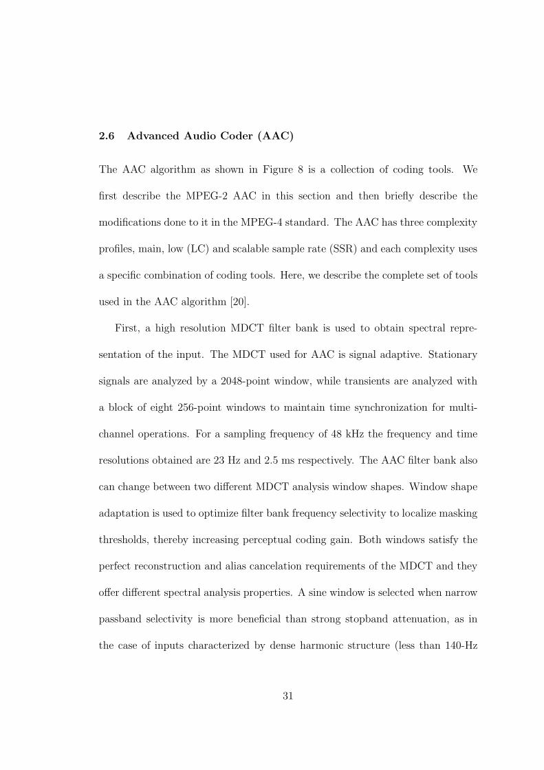
2.6 Advanced Audio Coder (AAC)
The AAC algorithm as shown in Figure 8 is a collection of coding tools. We
first describe the MPEG-2 AAC in this section and then briefly describe the
modifications done to it in the MPEG-4 standard. The AAC has three complexity
profiles, main, low (LC) and scalable sample rate (SSR) and each complexity uses
a specific combination of coding tools. Here, we describe the complete set of tools
used in the AAC algorithm [20].
First, a high resolution MDCT filter bank is used to obtain spectral repre-
sentation of the input. The MDCT used for AAC is signal adaptive. Stationary
signals are analyzed by a 2048-point window, while transients are analyzed with
a block of eight 256-point windows to maintain time synchronization for multi-
channel operations. For a sampling frequency of 48 kHz the frequency and time
resolutions obtained are 23 Hz and 2.5 ms respectively. The AAC filter bank also
can change between two different MDCT analysis window shapes. Window shape
adaptation is used to optimize filter bank frequency selectivity to localize masking
thresholds, thereby increasing perceptual coding gain. Both windows satisfy the
perfect reconstruction and alias cancelation requirements of the MDCT and they
offer different spectral analysis properties. A sine window is selected when narrow
passband selectivity is more beneficial than strong stopband attenuation, as in
the case of inputs characterized by dense harmonic structure (less than 140-Hz
31

spacing). On the other hand a Keiser-Bessell derived (KBD) window is selected in
cases for which stronger stopband attenuation is required, or when strong spectral
components are separated by more than 220 Hz [64][65]. The AAC also has an em-
bedded temporal noise shaping (TNS) module for pre-echo control (See Chapter
5).
The AAC algorithm realizes improved coding efficiency by applying prediction
over time to the transform coefficients below 16 kHz [49][50]. The bit alloca-
tion and quantization in the AAC follows an iterative procedure. Psychoacoustic
masking thresholds are first obtained as shown in the previous section. Both
lossy and lossless coding blocks are integrated into a rate-control loop structure.
This rate-control loop removes redundancy and reduces irrelevancy in one single
analysis-by-synthesis process. The AAC coefficients are grouped into 49 scale-
factor bands that mimic the auditory system’s frequency resolution, similar to
MPEG-1, Layer III [51][52]. A bit-reservoir is maintained to compensate for time-
varying perceptual bit-rate requirements.
Within the entropy coding block [53], 12 Huffman codebooks are available
for two- and four-tuple blocks of quantized coefficients. Sectioning and merging
techniques are applied to maximize redundancy reduction. Individual codebooks
are applied to time-varying sections of scale-factor bands, and the sections are
defined on each frame through a greedy merge algorithm that minimizes the bi-
trate. Grouping across time and intraframe frequency interleaving of coefficients
32

prior to codebook application are also applied to maximize zero coefficient runs
and further reduce bitrates.
For the MPEG-4 framework, the MPEG-2 AAC reference model was selected
as the “time-frequency” audio coding core. Further, the perceptual noise substi-
tution (PNS) scheme was included in the MPEG-4 AAC reference model. PNS
exploits the fact that a random noise process can be used to model efficiently,
the transform coefficients in noise-like frequency subbands, provided the noise
vector has an appropriate temporal fine structure [54]. Bit-rate reduction is re-
alized since only a compact, parametric representation is required for each PNS
subband rather than requiring full quantization and coding of subband transform
coefficients.
2.7 Bit-slice Scalable Arithmetic Coding
The concept of bit-sliced scalable arithmetic coding (BSAC) was introduced for
audio coding in [55] and is standardized as a part of MPEG-4 [20]. BSAC plays
the role of an alternative lossless coding kernel for MPEG-4 AAC, utilizing the
MDCT and applying a perceptually controlled bandwise quantization to the spec-
tral values. The main difference between BSAC and the standard AAC lossless
coding kernel is that the quantized values are not Huffman coded, but arithmeti-
cally coded in bitslices. This allows a fine grain scalability by omitting some
of the lower bitslices while maintaining a compression efficiency comparable to
33

the Huffman coding approach for the quantized spectral values. In the MPEG-4
AAC/BSAC codec the bitslices of the perceptually quantized spectral values are
already ordered in a perceptual hierarchy. In this way more perceptually shaped
noise is introduced as more and more bitslices are omitted.
34

3 TRANSFORM DOMAIN WEIGHTED INTERLEAVED VECTOR
QUANTIZATION
Transform-domain weighted interleave vector quantization (TWIN-VQ) is a
method used for compressing audio signals which has been found to be particu-
larly effective at low bit rates [56] [26]. Figure 9 shows block diagrams describing
the TWIN-VQ encoder and decoder. The input signal is first split into time frames
of 1024 samples. This frame is then transformed into the frequency domain using
MDCT
LPC Analysis
Side Information
Bark Scale
Analysis
Side Information
Weighted
VQOutput
IndicesInput
Signal
Inverse VQ
LPC Analysis
Side Information
Bark Scale
Analysis
Side Information
X IMDCTOutput
Signal
Input
IndicesX
(a) Encoder
(b) Decoder
:− :−
Figure 9: TWIN-VQ block diagram (a) Encoder (b) Decoder.
35

a 1024-point modified discrete cosine-transform (MDCT) while at the same time
the linear predictive coding (LPC) spectrum is calculated directly from the input.
The LPC spectrum provides a rough representation of the spectral envelope of the
MDCT coefficients, and it is used to normalize the MDCT coefficients to obtain
a flat spectrum by division in the MDCT domain. This is equivalent to perform-
ing linear predictive filtering and subtraction in the time domain to obtain the
residual error signal (i.e., the signal with the predictable portions removed). Fur-
ther normalization of the MDCT spectrum is done using the bark scale envelope.
Bark-scale envelope normalization is performed mainly to improve quantization
performance of signals with a lot of harmonic structure. Finally, quantization of
the final flattened spectrum is accomplished by using weighted interleave vector
quantization. The linear prediction coefficients and the power envelope from the
second flattening operation are also quantized and transmitted to the decoder as
side information.
The decoder simply inverts the steps of the encoder as illustrated in Figure 9.
The flattened spectrum is reconstructed from the VQ indices and the reconstructed
bark scale coefficients and linear predictive coefficients multiply this spectrum to
obtain an approximation of the original spectrum. A single frame of the time
domain audio signal is then reproduced by applying the inverse MDCT transform
to the reconstructed MDCT coefficients.
In the introduction, we stated that our intention is to modify the TWIN-VQ
36

algorithm to create a perceptually scalable audio coder. Note that it is only in the
quantization and encoding stage that psychoacoustic and statistical redundancy
are truly removed. Virtually all of the information removed by the prediction
stages in the encoder is added back to the signal in the decoder. It is thus this
stage that we must modify in the conventional TWIN-VQ algorithm to generate
a scalable bit stream. The quantizer in TWIN-VQ uses three main concepts: (1)
weighted vector quantization, (2) vector interleaving and (3) two-channel conju-
gate VQ [57] [58] [59]. We will discuss each of these in the following sections.
3.1 Weighted Vector Quantization
Weighted vector quantization (WVQ) is a VQ equivalent of adaptive bit allocation.
Adaptive bit allocation determines an optimal bit allocation scheme for a given
collection of random variables (the MDCT coefficients, in our case), based on the
variance of each random variable. The coding advantage or SNR improvement
obtained by using adaptive bit allocation is given by
G =
∑mi=1 λi
m∏m
i=i (λi)1
m
(18)
where λ2i is the variance of the ith variable. Optimal bit allocation works by
allocating bits to random variables proportional to their variances, but for percep-
tually optimal bit allocation the variances must be modified to take into account
the masking properties of the human ear.
37

x LPC
Code Book
VQIndexe
c
H
Figure 10: Vector quantization scheme for LPC residue.
A linear predictive coder (LPC) decorrelates successive samples in a signal.
For a vector x of successive samples [x[1], x[2], . . . , x[N ]]T , a linear predictor is
an FIR filter with coefficients hT = [h1, h2, . . . , hN ]. The filter coefficients can be
obtained by spectral factorization of the autocorrelation matrix R = E(xxT ) [21].
As shown in Figure 10, quantization is performed by finding the best code
vector c so as to minimize the distortion d between the input residual x and the
vector Hc, determined by synthesizing the residual codebook vector c. Here, H
denotes the impulse response matrix of the LPC synthesis filter: i.e.,
H =
1 0 · · · 0 0h1 1 · · · 0 0h2 h1 · · · 0 0...
... · · · ......
hm−1 hm−2 · · · h1 1
,
and we use HT to denote its transpose. If Euclidean distance is used, then dis-
tortion is given by
d = ‖x −Hc‖2. (19)
Assuming the power of the input vector x is normalized so that the residual
38

power is unity, we can write x as
x = He (20)
where e is the LPC residual vector. Replacing x in equation (19) with (20) we
get
d = ‖He −Hc‖2 = (e − c)THTH(e− c). (21)
Since H is a factor of the correlation matrix R of the vector x we can say
d = (e − c)TR(e − c). (22)
Because R is a positive definite matrix, we can diagonalize it with a unitary matrix
U that is composed of the eigenvectors of R
Λ = UTRU = diag[λ1, · · · , λm]. (23)
The eigenvalues λi are all non-negative and represent the variance of each random
variable in x. Rewriting the distortion d using (23), we have
d = (e − c)TUΛUT (e − c)
=∑m
i=1 λi(Ei − Ci)2
(24)
Equation (24) now represents the distortion as a weighted sum of the quantization
error between the transformed residual vector E and the transformed codevector
C: i.e.,E = UTe = [E1, E2, . . . , Em]T
C = UTc = [C1, C2, . . . , Cm]T .
39

The transformation UT is the Karhunen-Loeve transformation (KLT) for an au-
toregressive random process. Clearly, the quantization error in the transformed
domain, as computed in (24), is the same as that in the time domain as found in
(19). Thus, linear predictive quantization in the time domain can be represented
as a weighted vector quantization in KLT domain.
In this section, we want to quantify the quantization gain achieved by using
weighted vector quantization (WVQ). To do so, we first show that if a source is
uniformly distributed, the SNR gain due to WVQ matches the SNR gain for adap-
tive bit allocation in (18). Let x = [x1, . . . , xm]T be a m dimensional, uniformly
distributed vector with variances λ1, . . . , λm. Now, we introduce two vector quan-
tizer code books Cu and Cw that both contain the same number of codewords
and thus operate at the same bitrate of b. Codebook Cu is designed as a lattice
formed by uniform scalar quantization of each component xi of the vector x. If
the vector x is uniformly distributed over a hyper-rectangle of edge length Li with
respect to the component xi, then all of the VQ bins are hyper-rectangles of edge
size Li/N , where N = 2b, and the centroid is the corresponding codeword cu. The
average distortion for this case is given by
du =
∫ L1/N
0
· · ·∫ Lm/N
0
m∑
i=0
(xi − cui)2dx1 · · · dxm. (25)
Equation (25) is nothing more than the variance of the VQ bin normalized by
the total volume. The average distortion can also be written in relation to the
40

individual variances λi as
du = k
m∑
i=1
λi (26)
where
k =1
3
m∏
i=1
λ1/2i . (27)
Now, we construct the codebook for the weighted VQ Cw in a similar fash-
ion. In this case we use a lattice of uniform scalar quantizers with bi bits per
dimensional component xi. The optimal value of bi [21] is given by
bi = b +1
2log2
λi(
∏mi=1 λ
1
m
i
) (28)
and Ni the number of levels for the ith variable is given by Ni = 2bi. Using
the uniform quantization assumption and noting that the number of quantization
levels for index i is given by Ni = 2bi , the edge size of the ith VQ bin becomes
Li
Ni
= 2−bLi
∏mj=1 λ
1
2m
j
λ1
2
i
. (29)
Here, we use the weighted distortion integral to calculate the distortion instead
of the simple Euclidean distance-based distortion. Thus, the weighted distortion
is given by
dw =
∫ L1/N1
0
· · ·∫ Lm/Nm
0
m∑
i=0
λi(xi − cwi)2dx1 · · · dxm. (30)
which on simplification yields
dw = km
(
m∏
i=1
λ1
m
i
)
(31)
41

Thus, dividing (26) by (31) we can see that the coding gain for weighted VQ is
the same as that given for adaptive bit allocation (18).
3.2 Interleaving
So far we have analyzed the gain G obtained by using a WVQ. Now, we would like
to examine the relationship between the transform size m and the coding gain.
The correlation matrix R is a symmetrical Toeplitz matrix. In this case, the SNR
gain
SNG = 10 log10 G
can be explicitly expressed by the transform size m and PARCOR parameters pi
as follows [30]:
SNG = −10 log10
(
n∏
i=1
(1 − p2i )
m−im
)
. (32)
It can easily be shown that the linear prediction gain approaches this SNR
gain if the prediction filter size is large. This equation is useful for estimating the
relationship between the performance and the transform size. Since this estimate
holds for the time domain quantization procedure of (19), it is also useful for
estimating the performance of these coders in relation to the length of the delay
or the vector dimension.
As shown above, while a high SNR gain is expected for a large transform size
m, the vector dimension must be kept small for the following practical reasons.
At a fixed bitrate, computation complexity and the codebook size of the vector
42

quantization are exponentially proportional to the vector dimension. In order
to cope with these situations, it is necessary to split the full code vector c into
subvectors. If one splits it into J l-dimensional subvectors, SNR gain is given by
SNGs = 10 log10
(∑m
i=1 λi/m)(
∑Jj=1 dj/J
)
(33)
where dj is the geometric mean of the weighting factors for each subvector as
follows:
dj =∏
k∈Mj
λ1/nk
Mj denotes the index set of the elements which belong to the jth subvector.
In general, SNGs ≤ SNG, since the denominator of (33) is the arithmetic
mean of dj while that of 18 is the geometric mean of dj. However, equality holds
if dj is uniformly independent of j–i.e., even if the transform components are split
into subvectors, SNR gain remains unchanged provided that the geometrical mean
of the weighting factors for subvectors can be made equal.
Up to this point in our analysis, we have assumed that the transform used is
the KLT as described earlier. The KLT is not a general transform; it is specific
to a particular AR process. The TWIN-VQ algorithm, on the other hand, is
meant to deal with arbitrary audio signals, and thus uses the suboptimal (but
very effective) modified discrete transform (MDCT).
The complete set of MDCT coefficients passed to the VQ stage forms a very
large vector, typically in the range of 256-1024 elements within the TWIN-VQ
43

x1 x12x11x10x9x8x7x6x5x4x3x2
x1 x3 x5 x7 x9 x11 x2 x4 x6 x8 x10 x12
Figure 11: Interleaving a 12 dimensional vector into two 6 dimensional vectors
framework. Quantizing the whole MDCT coefficient set as a single vector is not
feasible because of the high computational complexity of the VQ index search and
the difficulty achieving a good design using algorithms like the generalized Lloyd
algorithm that generate only locally optimal solutions. The TWIN-VQ algorithm
overcomes these difficulties by splitting the large MDCT coefficient vector into
smaller sub-vectors such that the geometric mean of the weighting coefficients
corresponding to each sub-vector remains the same. This is done by decimating
the MDCT spectrum by the number of sub-vectors to be generated. For exam-
ple, if [x1, x2, x3, x4, . . . , xn−1, xn]T is an n dimensional vector, interleaving it into
two sub vectors would give the vectors [x1, x3, . . . , xn−1]T and [x2, x4, . . . , xn]T as
illustrated in Figure 11.
3.3 Two-Channel Conjugate VQ (TC-VQ)
The final quantization step in TWIN-VQ is performed using a technique called
two-channel conjugate VQ (TC-VQ). TC-VQ uses two different codebooks that
in some sense are “conjugates” of each other [58]. The TC-VQ encoder selects a
44

codebook vector from each of the two codebooks, calculates the average, and then
compares this average to a given input vector using a perceptually weighted mean
square distortion measure; i.e.,
d2 =
N∑
i=1
N∑
j=1
(
x − y1i + y2j
2
)T
W
(
x − y1i + y2j
2
)
. (34)
In the above equation, x is the input vector, y1 and y2 denote vectors from the
conjugate codebooks and W is a diagonal matrix with the perceptual weight
values along its diagonal. Indices of the pair of codebook vectors that minimize
the distortion are then transmitted to the decoder. A conjugate VQ structure has
much higher resolution than a normal codebook of the same size. As a simple
example, consider a TC-VQ codebook with N code vectors in each conjugate
codebook. The effective number of codevectors that can be represented is N2–
many more than the 2N codevectors that could be constructed using a simple VQ
codebook with the same number of elements. The length of the corresponding
channel codeword b is also reduced by half and the probability that the indices
of both output vectors are corrupted in transmission is significantly reduced. In
contrast, if only one codebook is used, the distortion significantly increases when
a transmitted code vector is lost.
For example, the SNR performance for a Gaussian source is approximately
proportional to the bitrate r per sample. The proportional constant in dB is
10 log10(4) or approximately 6 dB/bit. If the bitrate is reduced from r to r/2, the
45

SNR will decrease 3r dB. Thus, given a fixed bitrate, a two conjugate codebook
system results in reduced distortion when transmission errors occur compared to
a single codebook system.
3.3.1 Design of Conjugate Codebooks
Conjugate codebooks can be designed from a training set of vectors using an
iterative algorithm that is similar to the generalized Lloyd algorithm [21]. In this
method, both codebooks are simultaneously optimized by locally minimizing the
quantization distortion. The convergence of the algorithm is guaranteed because
the distortion is minimized at each iteration of the algorithm.
Any random codebook can be used as the starting point. If the improvement
in distortion becomes less than a threshold, the codebooks are considered to have
converged to the optimum.
1. Quantization of ui. For all training vectors ui, the best pair of intermediate
reconstruction vectors y1m and y2n is selected so as to minimize d from given
codebooks Y1 and Y2.
2. Fix codebook Y2 and renew codebook Y1. The new intermediate recon-
struction vector y1n is derived from the average distortion Dn for the old
y1n. The average distortion is given by
Dn =N∑
j=1
∑
ui∈y1n⊗y2j
‖ui −y1n + y2j
2‖2.
46

Quantization
D < Th
Renew
Centroids of
Y1
No
Yes
Stop
Initial Codebooks
Alternate
Renew
Centroids of
Y2
Figure 12: Conjugate codebook design algorithm.
To estimate the codebook vector in Y1 that minimizes the average distortion,
we differentiate it by y1n and equate to zero. The resulting expression for
the new codebook vector is
y1n = Ψ−1N∑
j=1
∑
ui∈y1n⊗y2j
(2ui − y2j),
where
Ψ =N∑
j=1
∑
ui∈y1n⊗y2j
1.
3. The above step is repeated, but this time the codebook Y1 is fixed, and
code vectors y2m are renewed.
4. The average distortion is checked and the process is stopped if the difference
in distortion falls below a particular threshold.
47

5. These above steps are repeated till the condition in the previous step is met.
The same training set is used for each iteration.
A simple flow chart for this process is as shown in Figure 12.
3.3.2 Fast Encoding for Conjugate VQ
In conjugate VQ, one codevector is chosen from each codebook to encode an input
vector. The chosen pair of codevectors should minimize the distortion. The most
straight forward method of searching for the best pair is to calculate the distortion
measure for all possible pairs, but this approach is not practical because of its high
computational complexity. For example, for a twin codebook of 32 codevectors
each, the number of distortion computations is on the order of 322 = 1024. To
overcome this problem, we use a fast encoding strategy which splits the encoding
process into two steps: pre-selection and main-selection.
During pre-selection, a fixed number of candidate codevectors are chosen from
a codebook and stored in a buffer where the number of candidates is less than the
codebook size. The candidates chosen are those most likely to result in the mini-
mum distortion and this procedure is performed separately for both the codebooks.
In the main-selection process, all pairs of candidates obtained in the pre-selection
process are combined, and their distortion measures are calculated. The pair giv-
ing the minimum distortion measure is chosen as the encoded output. Clearly the
main selection process is actually identical to the optimal encoding process except
48

that it operates on a smaller set of codevectors.
The pre-selection process can be further organized by performing an area-
localized pre-selection. Here, the codebook is divided into smaller sections, with
the number of sections being equal to the number of candidates in the preselection.
This organization of the codebook vectors within the candidate buffer simplifies
the programming and reduces the search complexity.
Finally, the computation can be further reduced by reusing parts of the pre-
selection process within main-selection. In the main-selection procedure, all pos-
sible pairs of pre-selection candidates are evaluated by the distortion measure,
based on the following equation
d2 = ‖y1 + y2 − x‖2 (35)
where, y1 and y2 are codevectors in the codebooks Y1 and Y respectively, and x
is the input vector to be encoded. Weighting factors have been omitted in (35)
for clarity, but the idea is identical for the WVQ case. Many of the computations
in the above equation can be split between the pre- and main-selection processes.
The method used to split the task of computing (35) is called hit zone masking.
To understand this method let us rewrite (35) as
d2 = ‖(y1n + y1p) + (y2n + y2p) − x‖2 (36)
where the subscript n and p denote the normal (perpendicular) and parallel com-
49

x
y1y2
Hit Zone
hit
Doesn't hit
hit
y1p y2p
d min
Figure 13: Hit zone masking method.
ponents of a vector. Mathematically this can be represented as
y = yn + yp (37)
where yn⊥y and yp‖y. Given that the inner product of normal vectors is zero,
(36) can be simplified to
d2 = ‖(y1n + y2n)‖2 + (‖y1p‖ + ‖y2p‖ − ‖x‖)2. (38)
The first term of (38) is always positive, so the distortion measure is always greater
than the second term, i.e.,
d2 ≥ (‖y1p‖ + ‖y2p‖ − ‖x‖)2. (39)
The hit zone masking exploits this characteristic. Figure 13 illustrates this method
with the current minimum distortion measure in the main-selection process ex-
50

pressed by dmin. The area between the parallel dashed lines is called the “hit
zone”. If the sum of two candidate vectors is outside the hitzone then the distor-
tion measurement for the pair is skipped since this pair cannot minimize dmin.
This hit-zone judgement can be determined by adding the parallel vector com-
ponents and this sum must be in the range ‖x‖ ± dmin to be in the hit zone.
Parallel vectors can be added with low computational complexity because this is
a scalar (i.e., element by element) operation.
The distortion measure for pre-selection within either code book is given by
d2p = ‖2y − x‖2
= 4‖y‖2 − 4y · x + |x‖2,(40)
where dp is the distortion measure. On the other hand, the distortion measure for
main-selection as described by (35) can be written as
d2 = ‖y1‖2 + ‖y2‖2 − 2y1 · x
−2y2 · x − 2y1 · y2 + ‖x‖2.(41)
Note that the first four terms of the above equation have already been calculated
for the pre-selection distortion measure. Thus, these terms can be saved after
the pre-selection step and reused during the main-selection. Furthermore, the
last term ‖x‖2 is calculated only once, and remains a constant throughout the
encoding process.
The coder proposed in this work uses the fast conjugate vector quantizers
described above. The fast encoder is especially useful here since we must encode
each critical band separately using multiple conjugate vector quantizers. Using a
51

full search quantization, the proposed scalable coder would not be feasible because
of the high computational complexity of its implementation.
52

4 REVERSE ENGINEERING THE TWIN-VQ
Developing a new, competitive audio compression algorithm is not an easy task.
In this work, we modify Twin-VQ as implemented in the MPEG 4 natural audio
coder reference software to create a scalable algorithm that is effective at low
bit rates [56][60]. The Twin-VQ tools in the MPEG 4 reference software was
developed by NTT corp., Japan. The training data used to design the VQs by
NTT has not, however, been made public. Therefore, the training set required to
design a scalable coder which is similar to Twin-VQ is not readily available. In
our case, we need a training set to design new VQs for each of the different critical
bands. In this chapter we describe a method to synthesize the required training
set from the original Twin-VQ codebook itself.
Vector quantizers are used primarily for data compression to speed transmis-
sion or to reduce storage requirements. In many compression systems, operations
like linear prediction, subband decomposition or wavelet transformation are car-
ried out prior to the use of VQ. Thus, the signal that is encoded by the VQ is
already represented in an efficient manner – i.e. with much of the signal energy
concentrated into a few coefficients. An optimal VQ codebook contains a great
deal information about an underlying data source model which can be extracted
and used to design a new codec having a different structure and yet optimized for
the same source model. The redesign process for a new VQ-based system involves
53

training the system again using either a set of collected signals or a probability
density function (pdf) that models the source of the signal. Since neither the
source pdf nor the original training set are available, we would normally have
to create our own training set of audio sequences. However, VQ codebooks opti-
mized for a particular training set does not necessarily work well for other training
sets. A simple experiment to demonstrate this is performed in the experimental
verification section. In the case of the Twin-VQ, the developers may have even
formatted the training data to give a more generalized representation of the un-
derlying source. Thus, a VQ designed over an arbitrary training set of available
audio sequences may not perform as efficiently as the original, highly optimized
Twin-VQ codebook.
A simple way to design a new VQ from an existing VQ is to transform the
codebook vectors of the old VQ in such a way that all pre-quantization processing
(e.g. transformations) are inverted. This technique works perfectly if the pre-
processing operations are linear and orthogonal. In particular, if a transformation
is orthogonal, the distance measure (the mean square error, MSE, for the VQ)
is preserved in the transform domain [21]. In this chapter, we discuss a method
to reverse engineer VQs for nonorthogonal transformations and to repartition the
VQ into multiple, lower dimensional VQs, each optimal for arbitrary subspaces of
the original codeword space. We then apply this method to Twin-VQ to create
separate vector quantizers for each critical band and thus allow for perceptual
54

scalability.
Our aim is re-engineer the TWIN-VQ coder to be scalable – i.e., to have a
layered quantization scheme in which each layer adds a small increment of fidelity
to the reconstructed audio signal. The first step in designing such a system is to
partition the VQ designed for original MDCT signal space into subspaces corre-
sponding to the different critical bands of human hearing (e.g. the bark scale)[32].
Note that partitioning of vectors into sub vectors can be viewed as a linear trans-
form in which distance is not preserved. Consequently, directly partitioning the
original codebook into subvectors corresponding to critical bands does not lead
to a good solution as we will show here. Instead, the reverse engineering scheme
proposed here turns out to be far more effective.
Most current image compression systems use transforms such as the DCT
(Discrete Cosine Transform) and the DWT (Discrete Wavelet Transform). These
transforms are either orthogonal transforms or close to orthogonal transforms (as
in the case of 9-7 or 5-3 biorthogonal wavelet transforms), so reverse engineering
them is straight-forward and does not require the approach developed here. We
note, however, that some of the new transforms that have been recently developed
for image compression like the contourlet and curvelet transforms are not even
close to orthogonal. Thus, the proposed reverse engineering scheme might be
highly effective when applied to these more recent compression systems.
In practical compression systems, VQ is often applied toward the end of the
55

Linear
TransformVQ
Losless
Compression
Input
Vectors
Output
Bitstream
(a)
Linear
Transform
VQ1Input
Vectors
VQ2
Subspace 1
Subspace 2
Output
Indices 1
Output
Indices 2
(b)
Figure 14: Block diagrams of a general VQ based compression systems. (a) sys-
tem that quantizes a transformed signal using VQ. (b) a system that quantizes
subspaces of the original signal separately.
56

encoding process and has the effect of reducing the bitrate of the signal represen-
tation dramatically. Most operations prior to the VQ are linear and deterministic
and they can almost always be easily inverted. Furthermore, these operations can
be identified and characterized simply by studying the decoder implementation.
Therefore, if we can synthesize a training set from the VQ codebook, we can
always pass each element in this set through the various inversion stages of the
decoder to create a training set for the original signal space (in our case, the space
containing all possible audio signals). In this chapter, we describe a method of
synthesizing a training set from a VQ and using it to design new VQ codebooks
for arbitrary spatial partitionings and transformations of the original vector (au-
dio signal) space. Figure 14 shows two notional compression systems using vector
quantization. In Figure 14(a) the original signal is transformed and the VQ is
applied directly to the transformed signal while in Figure 14(b) the signal vector
is split into two subvectors that are each fed into separate VQs, illustrating the
spatial partitioning for the vector space previously mentioned.
The most commonly used VQ design approaches are random coding, pruning,
pairwise nearest neighbor, splitting, and the Linde, Buzo, and Gray (LBG) or
the generalized Lloyd algorithm [21][61]. The common requirement for all these
algorithms is that they use a set of random samples (a training set) generated by
an underlying probability density function (pdf) rather than the pdf itself since
finding closed-form, optimal solutions is extremely difficult even when it is known
57

exactly. Therefore, the most straight forward way to reverse engineer a VQ is
to synthesize a training set whose statistics match those of the original training
set as closely as possible. The original codebook can be seen as a variable bin
histogram representing the original training set.
4.1 Training Set Synthesis
We need an accurate estimate of the underlying signal pdf to synthesize a good
training set. Furthermore, to simplify modeling on a computer the estimated
pdf should be a superposition of simple functions. Many techniques have been
proposed to estimate densities from training set data including nearest neighbor,
Parzen’s window and histograms [62][63]. The problem in our case is that the
amount of data available to us has been reduced to the number of elements in the
codebook by the LBG or some other clustering algorithm. The earliest density
estimation techniques developed for reduced data sets use the condensed nearest
neighbor rule (CNN) [64][65], and the technique is still of interest to researchers as
evidenced by recent work [29][66][67]. These techniques can be broadly classified
as nearest neighbor (NN) based techniques or Parzen’s window-based techniques.
Unfortunately, the NN-based techniques do not result in functions of known and
easily generated random variables that can be used to generate training vectors.
Parzen’s window estimators, on the other hand, provide a representation that is
a linear combination of simple pdf functions (e.g. “windows”) like Gaussian or
58

the uniform densities. To use a Gaussian window effectively, one must be able
to estimate the variance or, in the multidimensional case, the covariance matrix
of each window function [67]. Unfortunately, the VQ codebook does not contain
enough information to do this accurately. The obvious choice, then, is to use the
uniform window function which requires only a weight and the width/spread –
quantities that can be easily estimated from the polytope formed by each VQ bin.
Note that this approach is similar to the way in which variable bin size histograms
are designed [62]. A histogram measures the frequency of occurrence of vectors
in specific cells whose sum total partition the entire vector space (as defined by
the vectors of the training set), and the frequency of a particular cell is thus an
estimate of the probability mass of that cell. If the cell size is reduced (resulting
in an increase in the number of cells), the estimate converges asymptotically to
the pdf of the training set [29]. Consequently, the histogram of a training set
approximates the shape of the original pdf.
In our problem of synthesizing a representative training set, we are given only
the VQ codebook vectors and, if available, the entropy codes assigned to each
codebook index. To develop a synthesis methodology, we must study the VQ
design process. The main aim in the design of the VQ is to find a codebook
specifying the encoder that will maximize the overall performance as specified
by the statistical average over a suitable distortion measure. We use here mean
square error as our distortion measure. The encoder and decoder are completely
59

specified by the partition of the vector space into the cells R1,R2, . . . ,RN and
the codebook, C = {y1,y2, . . . ,yN}, respectively. Optimality for the partition
satisfies the nearest neighbor (NN) condition – i.e., for a given set of output
levels, C, the optimal partition cells satisfy
Ri ⊂ {x : d(x,yi) ≤ d(x,yj)} (42)
and the optimal code vectors for a given partition satisfy the centroid condition
given by
yi = cent(Ri). (43)
For the squared error or Euclidean distortion measure, the centroid of a set Ri is
simply the minimum mean square estimate of X given X ∈ Ri, i.e.
yi = cent(Ri) = E(X|X ∈ Ri) (44)
The conditions of (42) and (43) are the necessary but not sufficient conditions
for optimality of a VQ codebook and partition. By iteratively applying the two
conditions, one can obtain a VQ design that is at least locally optimal. As men-
tioned earlier, this VQ design procedure is similar to the problem of constructing
a variable bin histogram [29]. A variable bin histogram is generated by assuming
m cells A1, A2, . . . , Am, each characterized by the coordinate of the center xi and
the number of samples within each cell ki. In the VQ case, cells are characterized
by the VQ codebook entries and the partition rule. The only thing missing is the
60

number of samples within each cell. This, however, can be estimated from the
entropy codes assigned to each codebook entry since the entropy code depends
on the probability of the code word. Furthermore, the shape of the underlying
pdf of the training set is preserved in the spacing of the cells and in their shapes,
i.e., - the larger a cell, lower its probability density at any given point within it.
Given these assumptions, a training set can be synthesized by generating uni-
formly distributed vectors for each VQ partition. This requires us to generate
random variables distributed according to a constant density over the polytopal
partition cell. To create such random vectors, we first generate a uniform pdf over
a Cartesian grid which encloses the VQ cell. We then choose N vectors generated
by this pdf which fall inside the VQ partition. The following discussion justifies
this technique for generating uniformly distributed vectors within an irregularly
shaped polytopal region. Let U be the support of a uniform pdf p(x) and let S
be the uneven partition as shown if Figure 15. Here S is a proper subset of U and
L is the compliment of S with respect to U. The pdf p(x) can then be written as
p(x) = P1p(x|x ∈ S) + P2p(x|x ∈ L) (45)
where P1 and P2 are the probabilities that x ∈ S and x ∈ L, respectively. The
above equation can also be interpreted as a classification problem where the two
classes are S and L and the classes are mutually exclusive – i.e. there is no
intersection between the sets. Since the two classes are mutually exclusive, the
61

S
U
Figure 15: An irregular convex polytope S enclosed in the region of support for a
uniform pdf over the region U.
underlying pdfs must also be uniform. Thus, the vectors generated by p(x) within
the set S will be uniformly distributed in S. By synthesizing training sets for each
VQ partition according to the probability of the partition and combining these
sets, we generate a complete training set that has a histogram similar to that of
the original training set.
The following steps outline the proposed technique for synthesizing a training
set from a VQ codebook:
1. Assume that the original training set is large compared to the VQ codebook
size and that the number of number of elements in it is M . If indices are
entropy coded, we can estimate the probability of a codebook vector, p(yi)
62

since it is inversely proportional to the number of bits assigned to the code
vector. This probability estimate multiplied with M provides the number of
vectors in each partition. If an entropy coder is not used or if its parameters
are unknown, we instead assume that the number of vectors in each partition
cell is equal and given by Mk
where k is the number of code vectors in the
codebook.
2. For a given codebook vector yi, random vectors are generated as described
above such that they are uniformly distributed over the appropriate poly-
topal region.
3. The preceeding step is repeated for all the codebook vectors. The problem
of generating vectors for the overload region is side-stepped by confining
the problem to a finite region of support that depends on the number of
partitions and their sizes.
In the above approach, we assume that the Euclidean distance metric is used
in generating our training set. Euclidean distance d is defined as
d = (x1 − x2)T (x1 − x2) (46)
where x1,x2 ∈ Rk×1. In many coders, weighted distance measures are used to
make the VQ a more efficient. A weighted distance measure is given by
d = (x1 − x2)TW(x1 − x2) (47)
63

where W. A property of a distance measure is that it is always non-negative, i.e.
d = (x1 − x2)TW(x1 − x2) ≥ 0. (48)
This implies that W has to be positive semidefenite and it can thus be written as
W = RTR = UT ΛT1/2Λ1/2U (49)
where U is a unitary matrix with eigenvectors of W as its columns and is a
diagonal matrix with the eigenvalues of W as its diagonal elements. Consequently,
the weighted distance measure can be written as
d = (x1 − x2)TRTR(x1 − x2) (50)
which is nothing but the Euclidean distance in the space transformed by the
matrix R. Therefore to synthesize the training set for a VQ designed using a
weighted distance metric like that used in [56] or [26], we need only construct the
training set as above and transform all the synthesized vectors by the matrix RT .
4.2 Theoretical Analysis
In the approach of the previous section, we approximate a pdf within a VQ par-
tition cell as uniform. Here, we justify this choice. In the reverse engineering
problem which motivates this work, we do not know the shape of the underlying
pdf within the codebook partition. Our goal in this section is to characterize the
error incurred when we use the uniform density approximation outlined above in
64

place of the unknown, underlying pdf. Note that this error is equivalent to the
variance of the truncated pdf which describes the source distribution within the
partition.
For a multidimensional pdf over a convex polytopal region, we can claim the
following: (1) the mean vector is composed of the means of the marginal pdfs of
the given multidimensional pdf in all dimension and (2) the variance (distortion
with respect to the centroid) is the sum of the variances of the marginal pdfs.
During VQ design, the partitions are formed such that the distortion in a given
region is minimized. Assuming that the underlying pdf can be represented as a
Gaussian Mixture Model (GMM), and that the number of codebook vectors is
greater than the number of modes in the mixture, we can say that in most cases
the pdf over a VQ partition is denser near the centroid (i.e. the mean). Thus,
we can assume that in most partitions, the marginal density functions are either
unimodal or monotonically increasing or decreasing functions. There could also
be cases where the probability density is large closer to the edges of the polytope,
thereby having marginal densities with minima close to the mean. These cases
would be very rare, however, if we assume a reasonably large codebook size.
Following the above discussion, we can thus characterize the variance (the mean
square distortion in our case) of a multidimensional pdf confined to a polytopal
region by characterizing the variances of the marginals.
For a given VQ codebook, we assume that the underlying pdf is smooth.
65

Consequently, we can further assume that the marginal pdfs are smooth and are
defined over a finite interval [a, b] on the real line. Our problem then becomes one
of comparing the variance of a one dimensional uniform density function to that
of unimodal and monotonic density functions over a fixed interval. Seaman and
Jacobson have independently shown that the variance is maximized by the uni-
form density for a set of unimodal functions (with some constraints)[68][69]. For
the monotonic case, we first consider two examples: (1) a set of linear monotonic
decreasing functions and (2) a set of truncated exponentials with varying conver-
gence rates. For the set of linear monotonic functions, it is easily shown that the
uniform density has the maximum variance. The set of linear monotonic functions
can be defined as
f(x) = (1 + e) − 2ex (51)
over the interval [0,1], where e is a value in the interval [0,1] and when e = 0, the
function is the uniform density function. An example of this function is as shown
in Figure 16. The variance of this function is given by
V ar(x; f(x)) =1
12− e2
36(52)
and therefore
V ar(x; u(x)) =1
12≥ V ar(x; f(x)) (53)
where u(x) is the uniform density over the interval [0,1]. This logic can be extended
to any finite interval on the real line. Considering now case (2), the pdf for the
66

set of truncated exponentials can be written as
f(x) =
(
b
(1 − exp(−b))
)
exp(−bx) (54)
where the parameter b controls the rate of convergence of the pdf over the interval
[0,1]. The interval over [0,1] is taken simply for convenience and can be easily
extended to any other interval on the real line. Figure 17 shows a plot of the
variance of the truncated exponential with respect to the parameter b. From this
plot, we can see that the variance of the uniform pdf (the broken line in the figure)
upper bounds only a certain subset of the truncated exponentials – specifically,
for 0.05 < b < 4.5. Nevertheless, we can still say that the variance of a one di-
mensional uniform density function (over a fixed interval) forms an upper bound
with respect to the variances of a large set of unimodal and monotonic density
functions defined over a common finite interval. Extending this to the multidi-
mensional case using the marginal density argument of the previous paragraph,
we can further say that the uniform density over a fixed polytopal region is likely
to have higher variances and therefore form an upper bound on the distortion
relative to that incurred using the true (unknown) pdf.
In the previous paragraphs, we showed that if the distortion computed using
uniform density approximation over each partition provides an upper bound rel-
ative to the distortion in some common situations. Thus, the true rate distortion
performance is likely to be better than the operational R-D performance esti-
67

1 - e
1
1 + e
10
f(x)
Figure 16: Plot of linear monotonically decreasing function. The parameter e
controls the slope of the pdf.
mated for the synthesized training set. It has been shown that as the number of
partitions is increased, the probability density in each partition approaches that
of the uniform density function [70]. This implies that as the number of partitions
is increased (i.e., the size of the codebook is increased), the upper bound on the
distortion converges to the distortion integral of the true underlying pdf [71][72].
The rate at which this convergence occurs can be demonstrated as follows. Let
f(x) be a mixture of k Gaussian densities and x ∈ Rn. If we design a VQ for
f(x) assuming negligible overload distortion and k codebook vectors, an optimal
VQ would very likely place a codebook vector at the mean of each Gaussian in
the GMM. Each VQ cell is then a convex polytope with the mean of a Gaussian
68

0 1 2 3 4 5 6 7 8 9 100
0.02
0.04
0.06
0.08
0.1
0.12
0.14
0.16
0.18
0.2
parameter b
Var
ianc
e
Figure 17: Plot of variance of the truncated exponential with respect to the rate
parameter b. The broken line is the variance of a uniform pdf over the same
interval.
69

element as its centroid. If we increase the number of codebook vectors, the sizes
of the VQ cells at the modes of the Gaussian components decrease and new VQ
cells are introduced covering the tails of the Gaussian components. Our goal is to
show that if the number of VQ cells is increased then the shape of the conditional
pdf over each partition rapidly approaches that of the uniform density. To do this,
we first show that the conditional pdf on a VQ cell centered at the mode rapidly
converges to the uniform density. Consider a one dimensional Gaussian pdf with
zero mean and variance σ2 truncated in the interval [-1, 1] and given by
g(x) =1
p√
2πσ2exp
(−x2
2σ2
)
(55)
where p is a normalizing factor ensuring that∫ 1
−1g(x)dx = 1. If h(x) is a uniform
pdf over the interval [-1,1], then the mean square error (MSE) between h(x) and
g(x) is given by
d =
∫ 1
−1
(g(x) − h(x))2dx =
∫ 1
−1
(g2(x) + h2(x) − 2g(x)h(x))dx (56)
which is found to be equivalent to
d =erf
(
1σ
)
2[
erf(
1√2σ2
)] (57)
where the erf function is the Gaussian error function. Therefore, d is a monoton-
ically decreasing function with respect to σ. A plot of d versus the standard de-
viation σ is shown in Figure 18. We see from the plot that as the variance is
increased, the pdf over the fixed interval rapidly converges to that of the uniform
70

0 5 10 15 20 25 30 35 40 45 500
0.002
0.004
0.006
0.008
0.01
0.012
Variance
Dis
tort
ion
d
Figure 18: Plot of the mean square error between a truncated Gaussian and a
uniform pdf over a fixed σ2.
density. This analysis extends directly to multiple dimensions as follows. Let p(x)
be a truncated Gaussian within a polytope V, with mean 0 and covariance matrix
R for x ∈ Rn. Its density is thus given by
p(x) =exp
(
−xT Rx
2
)
∫
Vexp
(
−yT Ry
2
)
dy(58)
The covariance matrix is a positive definite matrix, hence we can represent it in
its spectral form as
R = UTΛU (59)
where U is a matrix with the eigenvectors of R as its columns and the diagonal
matrix Λ contains the eigenvalues of R. Now, by rotating the coordinates of
71

the space such that the eigenvectors align with the coordinate axes, the pdf will
be separable, and the diagonal elements of Λ can be viewed as the variances of
the Gaussian pdfs along each coordinate axis. Clearly, as the eigenvalues of R
increase, R−1 = UTΛ−1U converges to a matrix with all its elements equal to
zero. This implies that in the limit as the eigenvalues go to infinity, the pdf
described in (58) goes to
p(x) =1
∫
Vdy
= h(x) (60)
which is the uniform distribution over the polytope V . Note that increasing the
variance of the truncated Gaussian is completely analogous to reducing the size of
the region of support while keeping variance constant. This is what occurs when
the number of VQ partitions is increased.
4.3 Smoothed Training Set Synthesis
For a moderate to large codebook size N , the rate-distortion curves for the synthe-
sized codebooks converge rapidly to those of the true codebooks with increasing
N . For smaller values of N , however, a training set corresponding to a smooth
PDF approximation should provide better performance. Such a training set can
be synthesized with only small changes to proposed approach. The specific steps
are as follows:
1. From the original VQ codebook, we synthesize a training set as in Section
72

3.2. This results in a training set that has been implicitly generated by a
piecewise uniform density model.
2. To smooth the underlying piecewise uniform PDF, we use a Parzen’s window
function; specifically, a Gaussian window given by:
ϕ(x) =1√2π
exp
(−xT Rx
2
)
(61)
3. To generate a training set that has a smoothed pdf we take the synthesized
training set as in step 1, say Y = {y1,y2, . . . ,yM}, and synthesize new
training set vectors X = {x1,x2, . . . ,xM} distributed according to a PDF
given by
xi ∼ ϕ(x) =1√2π
exp
(−(x − yi)TR(x − yi)
2h
)
(62)
where h is a smoothing factor – the larger the value of h, the smoother the
estimated PDF. While smoothing does not add a lot of computational complexity
to training set synthesis, it does necessitate the generation of larger training sets
in order to accurately represent the smooth underlying PDF.
4.4 Reverse Engineering TWIN-VQ
As detailed in chapter 3, the Twin VQ algorithm uses vector interleaving and
two-channel conjugate codebooks. Thus, to obtain a training set representative of
the MDCT coefficients, we need to first obtain a training set that represents the
73

Index Gen.
Codebook 1
Index Gen.
Codebook 2
Vector
Synthesizer
Vector
Synthesizer
+ Interleaved
Vectors
Deinter-
leaving.
.
.
Interleaved
Vectors Synthesized
MDCT Spectrum
Figure 19: MDCT frame training set synthesis.
two conjugate VQs. The training sets for the conjugate VQs are then combined
randomly to form the interleaved vectors, and these interleaved vectors, are dein-
terleaved to obtain a frame of MDCT coefficients. The two channel conjugate VQ
used in the MPEG-4 Twin VQ has two codebooks of 174 codebook vectors each.
Generating a training set and obtaining all the possible combinations of the train-
ing set vectors prior to deinterleaving poses a major challenge. As an example if we
directly combine the conjugate VQ codebooks there are about 174× 174 different
combinations possible – too large a number for the synthesis procedure outlined in
the previous section to handle efficiently. To overcome this difficulty, we generate
the MDCT coefficient vector one at a time as discussed in the paragraphs that
follow.
74

The block diagram as shown in Figure 19 illustrates the procedure proposed
to obtain training set samples for the flattened MDCT spectrum. A random
number generator first selects an index for each of the two conjugate codebooks,
useing the probability information obtained from the Huffman coding tool. These
indices are then passed to a vector synthesis block which generates random vectors,
uniformly distributed over the quantization bin of the specified codebook vector.
Combining the vectors generated for each conjugate codebook, we obtain a single
interleaved vector. Since Twin VQ decomposes the 1024 size MDCT frame into 64
different interleaved subvectors, we must generate 64 different interleaved vectors
as described above and then deinterleave them to obtain a single training set vector
for the MDCT frame. This technique is statistically equivalent to the training set
synthesis procedure mentioned in the previous section, but it saves memory space
and computation by generating one MDCT spectrum vector at a time.
4.5 Experimental Verification
4.5.1 Operational Rate Distortion Curves
In this section, we present some numerical examples to demonstrate the perfor-
mance of the proposed training set synthesis method. In the following experi-
ments, we evaluate the rate distortion curves for different scenarios, comparing
the original and synthesized VQs. We assume here that the underlying source pdfs
are either Gaussian pdfs or mixtures of Gaussians, and we note that the distortion
75

integrals are calculated using the spherical invariance property of the Gaussian
and a Monte Carlo technique proposed by Deak [73][74]. Figure 20 shows the op-
erational rate-distortion (RD) curve assuming that the original source training set
is generated by a symmetric 3-Dimensional Gaussian pdf. Here, the new training
set is synthesized assuming that the probability of each VQ codebook vector is
known (i.e. that we have access to the entropy codes). From the figure, we see that
the distortion decreases with the bit-rate and that the curves for the synthesized
and original designed VQ are very close together, beginning to converge at higher
rates. To illustrate this more precisely, we compare in Figure 21 the two opera-
tional rate-distortion curves from Figure 20 by taking their ratio. We also plot
the 95% confidence intervals. From this plot, we see that the ratio is significantly
greater than one for small codebook sizes, indicating that the synthesized VQ is
greatly inferior to the directly designed VQ, but we note that it tends to unity as
the codebook size is increased, illustrating the expected asymptotic convergence.
The same experiment is repeated for a 2-dimensional Gaussian Mixture Model
with three Gaussian components, and the ratio of the RD curves for the original
versus the synthesized codebooks is plotted in Figure 22. In this case, however,
we plot ratios for both the smoothed and unsmoothed synthesized codebooks. As
expected, smoothed training set synthesis performs considerably better than un-
smoothed synthesis for smaller codebook sizes, but it performs equivalently once
the codebook size exceeds 60.
76

10 20 30 40 50 60 70 80 90 1000.3
0.4
0.5
0.6
0.7
0.8
0.9
1
1.1Synthesized TSOriginal TS
Figure 20: Plot of Rate (VQ codebook size) vs. the Distortion in Mean Squared
Error for a symmetric Gaussian pdf assuming prior knowledge of the probabilities
of VQ codebook vectors.
77

The examples above have illustrated both the utility of training set synthesis
for VQ redesign and the speed with which it converges to the optimal solution as
the codebook size increases. Our real interest, however, is in redesigning VQs for
subspaces or transformed spaces of the original signal space – e.g., repartitioning it
to describe the different subspaces formed by grouping together different elements
of the original vector space. Once we have the synthesized training set, all we have
to do to design the new subspace VQs is transform each of the training vectors
into the appropriate space. This is much easier than directly transforming a PDF.
To illustrate our approach, we perform two experiments. In the first experiment,
we redesign a vector quantizer for a linearly transformed (non orthogonal) space
while in the second, we create separate VQs for subspaces of the original vector
space.
4.5.2 Transformed Space Vector Quantization
The contourlet transform is most commonly applied to images and is used to ef-
ficiently represent the edges within and image that have orientations other than
the horizontal and vertical [75]. This contourlet transformation is implemented
by first performing a pyramidal decomposition, and then applying a directional
filter bank on the high frequency components of the image. In the following ex-
periment we assume that we are already given a VQ-based scheme that encodes
512x512 grayscale images, where each vector is formed by 8x8 pixel blocks. The
78

0 20 40 60 80 100 1200.9
0.95
1
1.05
1.1
1.15
1.2
1.25
Rate N
Dis
tort
ion
Bia
s
Figure 21: Plot of the rate (VQ codebook size) versus the ratio of distortion in
mean squared error for a symmetric Gaussian pdf assuming prior knowledge of
probabilities of VQ codebook vectors.
79
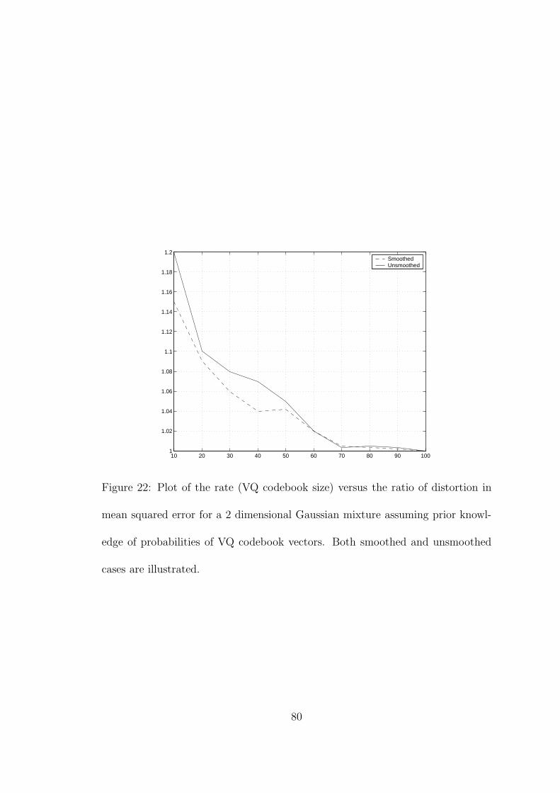
10 20 30 40 50 60 70 80 90 1001
1.02
1.04
1.06
1.08
1.1
1.12
1.14
1.16
1.18
1.2SmoothedUnsmoothed
Figure 22: Plot of the rate (VQ codebook size) versus the ratio of distortion in
mean squared error for a 2 dimensional Gaussian mixture assuming prior knowl-
edge of probabilities of VQ codebook vectors. Both smoothed and unsmoothed
cases are illustrated.
80

VQ is trained from the standard Lena, Barbara and Boats images and contains
256 codevectors. We wish to design a new image compression system that ap-
plies the contourlet transform on 8x8 pixel blocks of the original image and then
uses a VQ to compress the different high frequency directional components. The
simplest way to do this is to form new codebooks by directly transforming the
original codebook. Let us call such a codebook the ’extracted codebook’. As an
alternative, we design new codebooks from the original codebook using the pro-
posed training set synthesis approach. To do this, we first synthesize a training set
from the original codebook, transform the training set using the contourlet trans-
formation, and finally design new codebooks for each of the transform coefficient
vectors.
For the experiment presented here, the contourlet transform is performed us-
ing the Contourlet Toolbox developed by Minh Do [76]. The pyramidal filter bank
and the directional filter banks are implemented using the 5-3 wavelet transform,
and a three stage pyramidal transform is used to decompose the image into three
different frequency subbands (one low and three high frequency subbands). The
three higher frequency bands are further decomposed into 3, 8 and 16 directional
subbands respectively. In the experiment presented here, we consider quantiza-
tion of only the two different directional subbands obtained by doing a directional
decomposition on subband-3. We label these directional subband-1 and direc-
tional subband-2. Note that the collective transform (from pyramidal filtering to
81

Table 1: Comparison performance (in MSE) between VQs designed using the
original training set and the synthesized training set for linearly transformed data.
Directional Optimal Extracted Synthesized SynthesizedSubbands Redisign Codebook Codebook with Codebook without
Probability ProbabilityDirectional 11.32 24.82 16.28 20.92Subband 1Directional 9.23 21.20 14.44 20.57Subband 2
directional decomposition) forms a highly non-orthogonal transform – a case for
which direct codevector transformation is not likely to be effective.
Given a training set, one can design VQs for any desired bit-rate. In this
example, we design each of the new (lower dimensional) codebooks at the same
rate as the original codebook so that the total bit-rates of both codes are the same.
This results in codebooks that contain 256 code vectors each. Table 1 compares
the mean square distortion for the two directional component vectors and four
different cases - optimal redesign using the original training set, new codebooks
that are directly extracted from the original codebook, and training set synthesis
with and without entropy codes. We can see from the table that the synthesized
VQ performs much better than the extracted VQ. Specifically there is 19-34%
reduction in the distortion using the synthesized codebooks versus the directly
extracted codebook vectors.
82

4.5.3 Partitioned Space Vector Quantization
In the next experiment, we design VQs for subspaces formed by repartitioning
the original vector space into lower dimensional subspaces. If x is a vector
such that x ∈ Rn with elements x = [x1, x2, . . . , xn]T , this vector space can
be repartitioned simply by regrouping its element as x1 = [x1, x2, . . . , xl]T and
x2 = [xl+1, xl+2, . . . , xn]T for some integer l < n. Here, we generate the original
training set distributed as a four dimensional, bimodal Gaussian mixture density.
The location of the modes m1, m2 of each Gaussian density element are given by
m1 = [0000]T and m2 = [2321]T , respectively, and the covariance matrices R1,R2
are given by R1 = I (identity) and
R2 =
1 0.3 0.1 00.3 1 0.3 0.10.1 0.3 1 0.30 0.1 0.3 1
The first two elements of the original four dimensional vector are mapped to sub-
space 1 and the remaining elements to subspace 2. The VQ codebook for the
full space is initially designed from the original training set using the LBG al-
gorithm - we call this codebook the original codebook. The original training set
contains 1000 vectors and the original codebook size is 20 vectors. As in the pre-
vious example, we consider two ways of designing the new codebooks: (1) directly
partition the original codevectors into the required subspaces and (2) using the
proposed approach to synthesize a training set, partitioning the training set into
subspaces and then redesigning the codebooks for the corresponding subspaces.
83

Table 2: Comparison of performance (in MSE) between VQs designed using the
original training set and the synthesized training sets for subspace vectors.
Subspace Optimally Extracted Synthesized Synthesized SmoothedRedesigned Codebook With Without synthesis
Probability Probability withProbability
Subspace 1 0.30 0.40 0.33 0.36 0.34Subspace 2 0.23 0.39 0.27 0.33 0.25
We consider here both smoothed and unsmoothed training set synthesis, and we
synthesize a training set containing 1000 vectors from the original codebook. After
repartitioning each element of the training set into two two-dimensional vectors,
new codebooks are designed for each subspace from these two synthesized sets.
Finally, the codebook for each subspace contains 20 codevectors, maintaining the
original code rate and allowing us to easily compare this system with that formed
by directly partitioning the original codebook vectors into subvectors (labeled ’ex-
tracted codebook’ in Table 2). The MSE performances are compared in Table 2.
Studying the table, we note that the gain in performance achieved using training
set synthesis instead of codebook extraction is significant – 9.5% to 16% for sub-
space 1 and 16.5% to 32% for subspace 2, depending upon the availability of code
vector probabilities. Comparing smoothed and unsmoothed synthesis, we see that
their relative mean squared errors are essentially the same: smoothing performs
slightly worse on Subspace 1 and slightly better on Subspace 2.
We note, however, that for the results of both experiments, the performance
84

of training set synthesis is far below that achieved when the VQ is optimally
redesigned using the original training set. With codevector probabilities, the
average increase in MSE for the contourlet example is about 50% while for spatial
partitioning it is about 19%. While these numbers may seem high, it is important
to note that optimal redesign requires information (e.g. the original training
set) which is unavailable to us. We present these comparisons here primarily to
quantify how close the performance of the proposed training set synthesis approach
is to that of the best possible codebook (e.g. to the upper performance bound).
4.5.4 Performance of training set synthesis within the TWIN-VQ frame-
work
In our final experiment, our primary goal is to evaluate the performance of training
set synthesis for the redesigned TWIN-VQ – we are not considering here the
problem of scalable compression which will be addressed in the next chapter.
Thus, for this experiment, we fix the output bitrate of the encoder to 16 kb/s.
Since we have found that the most perceptually significant information lies within
the first 18 critical bands or bark levels when coding at this bit rate, we design
only 18 residual VQs. Each of the VQs must therefore operate at a rate of 0.5
bits per sample.
These different VQs are designed from two different training sets: (1) the
training set obtained from randomly chosen audio sequences and (2) the training
85

Table 3: Sequences used for the TWIN-VQ experiment.
Sequence No. Sequence Genre DurationName (seconds)
1 Cliff Richards Rock 202 Korn Rock 203 Benetar Rock 104 Erick Clapton Rock 155 Beethoven 9th Classical 206 Swan Lake Classical 207 Nut Cracker Classical 208 Cinderella Classical 20
set synthesized by the method described in section 4.4. Specifically, we compare
training set synthesis to two different training sets obtained from random audio
samples. The audio sequences used for training are listed in Table 3. The first four
are 20s sequences of rock music and the last four are 20s sequences of classical
instrumental music. The first training set is obtained from sequences 1 and 2
and the second training set is obtained from sequences 5 and 6. Finally, the
actual training vectors are obtained by applying an MDCT followed by the 2-
stage TWIN-VQ prediction process using the TWIN-VQ tool of the MPEG-4
audio reference software [20]. The synthesized training set, on the other hand,
is derived from the codebook of the TWIN-VQ MPEG-4 tool as described in
section 4.4. All the three training sets contain 2000, 1024-dimensional vectors
which are partitioned into the different critical bands. The residual VQs for each
critical band are then designed from each of these different training sets and the
remaining of the sequences within each genre (i.e., those not used in the VQ design
86

Table 4: Comparison of performance (in MSE) between TWIN-VQ systems de-
signed using random audio data and synthesized training set from the MPEG-4
standard.
Genre VQ designed VQ designed Synthesized Extractedfrom from from Codebook
Seq.1 and 2 Seq. 5 and 6 MPEG-4TWIN-VQ
Genre 1(Rock) 0.44 0.83 0.49 0.75
Seq. 3 and 4Genre 2
(Classical) 0.67 0.53 0.50 0.73Seq. 7 and 8
process) are encoded.
The weighted mean square error results for the VQs designed from each of
the training sets are as shown in Table 4. The weighting values are calculated
from the LPC spectrum and bark scale spectrum of the sequences being encoded
in the same manner as in the TWIN-VQ encoder. From the first two columns,
we see that the average distortion is much lower when the VQs used to encode
sequences are designed using sequences of the same genre. However, the set of
VQs designed by training set synthesis perform equally well for both the genres
and is 36-69% better compared to the directly designed VQs when the genres are
mismatched. Furthermore, training set synthesis has on the average a 33% lower
MSE compared to direct codebook extraction. Clearly, the training set synthesis
method results in a far more effective VQ over the unknown original training set
87

than the alternatives. In reality, of course, it is subjective audio quality that
really matters in this application. Extensive subjective testing is presented in
subsequent chapters.
88

5 SCALABLE TWIN-VQ CODER
Before we discuss our scalable Twin-VQ coder, we first present two important
tools used in its construction: the modified discrete cosine transform and temporal
noise shaping. The modified discrete cosine transform (MDCT) is used for time-
frequency analysis within Twin-VQ, allowing critical bands to be extracted from
the MDCT spectrum. On the other hand, non-simultaneous coding artifacts like
pre-echo (described in section 5.2) are reduced by using the temporal noise shaping
(TNS) tool.
5.1 Modified Discrete Cosine Transform
Cosine-modulated pseudo quadrature mirror filter banks (PQMF) have been used
to create M-channel filter banks with almost perfect reconstruction properties
[77][78][79]. Cosine modulated filter banks use a single lowpass, finite impulse
response (FIR) prototype filter and modulate it to obtain bandpass filters. The
PQMF banks have some nice properties such as, overall linear phase, uniform
subband widths, low complexity of construction (one FIR filter and modulation)
and critical sampling.
In the PQMF bank derivation, phase distortion is completely eliminated since
by forcing the analysis and synthesis filters to satisfy the mirror image condition,
gk[n] = hk[L − 1 − n], (63)
89

where gk[n] and hk[n] are the analysis and synthesis filters for the kth band.
Adjacent channel aliasing is eliminating by establishing precise frequency domain
positioning of the analysis and synthesis filters Hk(z) and Gk(z), respectively.
After critical sampling, these conditions yield analysis filters given by
hk[n] = 2w[n] cos
(
π
M(k + 0.5)
(
n − (L − 1)
2
)
+ θk
)
(64)
and synthesis filters given by
gk[n] = 2w[n] cos
(
π
M(k + 0.5)
(
n − (L − 1)
2
)
− θk
)
(65)
where
θk = (−1)k π
4
and w[n] corresponds to an L-length, real coefficient, linear phase FIR prototype
lowpass filter, with normalized cutoff frequency π/2M . Thus, the filter bank
design is equivalent to designing the window w[n].
The PQMF filterbank is not perfect reconstruction (PR). It is useful in audio
coding applications to restrict the quantization distortion to specific frequency
bands to a specific instance in time. Malvar and Vaidyanathan have independently
shown that it is possible to have PR cosine modulated filterbanks [77][78]. This is
done by appropriately constraining the synthesis filters gk[n], for 0 ≤ k ≤ M − 1.
Here, we are interested in the MDCT which is a cosine modulated filterbank with
L = 2M , where L is the length of the prototype filter and M is the number of
90

analysis filters. The MDCT analysis filter impulse responses are given by
hk[n] = w[n]
√
2
Mcos
(
(2n + M + 1)(2k + 1)π
4M
)
(66)
and the synthesis filters are obtained by time reversing the analysis filters, i.e,
gk[n] = hk[2M − 1 − n] (67)
this is done so as to satisfy the overall linear phase constraint. While the above
equations give the impulse responses of the analysis and synthesis filters for the
MDCT, it is more typical to implement this transformation in a block form.
The MDCT analysis filterbank is implemented using a block transform of
length 2M samples and is advanced by M samples. This implies that two adjacent
blocks have an overlap of M samples (50%). Thus, the MDCT basis functions
extend across two blocks in time, thereby virtually eliminating blocking artifacts.
The MDCT is a critically sampled tranform, i.e., with a 50% overlap only M
coefficients are created by the forward transform for each 2M-sample input block.
Given an input block x[n], the transform coefficients X[k], for 0 ≤ k ≤ M − 1 are
given by
X[k] =
2M−1∑
n=0
x[n]hk[n]. (68)
The MDCT analysis performs a series of inner products between the M analysis
filter impulse responses hk[n] and the input x[n]. On the other hand, the inverse
MDCT obtains a reconstruction by computing a sum of basis vectors weighted
91

by the transform coefficients from two blocks. The first M-samples of the kth
basis vectors, hk[n], for 0 ≤ n ≤ M − 1, are weighted by the kth coefficient of
the current block, X[k]. Simultaneously, the second M-samples of the kth basis
vector, hk[n], for M ≤ n ≤ 2M − 1, are weighted by the kth coefficient of the
previous block X ′[k]. Then, the weighted basis vectors are overlapped and added
at each time index n. Note that the extended basis functions require the inverse
transformation to contain an M-sample memory in order to retain the previous
set of coefficients. Thus, the reconstructed samples x[n], for 0 ≤ n ≤ M − 1, are
obtained by the inverse MDCT, defined as
x[n] =M−1∑
k=0
(X[k]hk[n] + X ′[k]hk[n + M ]) . (69)
The analysis and synthesis filters for the MDCT are derived from a prototype
FIR filter w[n]. The generalized PR conditions when applied to the prototype
filter yields the constraints
w[2M − 1 − n] = w[n], and
w2[n] + w2[n + M ] = 1,(70)
for sample indexes 0 ≤ n ≤ M − 1. Several windows have been proposed
[80][81][82][83]. The most commonly used window function for audio is the sine
window, defined as
w[n] = sin
[(
n +1
2
)
π
2M
]
(71)
for 0 ≤ n ≤ M − 1. This window is used in standards like MPEG-1, Layer 3
(MP3), MPEG-4 AAC, and Twin-VQ.
92

5.2 Temporal Noise Shaping
Pre-echo distortion arises in transform coding systems which use perceptual coding
rules. Pre-echoes occur when a signal with a sharp attack begins near the end of
a transform block immediately following a region of low energy. Since masking
thresholds are calculated and applied in the frequency domain, the quantization
noise that is introduced in the frequency domain spreads evenly throughout the
reconstructed block due to time-frequency uncertainty. This results in unmasked
noise throughout the low energy region preceding the signal attack at the decoder.
Temporal noise shaping is a frequency domain technique to counter the effect
of pre-echo distortion [84]. A linear prediction (LP) is applied across the frequency
(rather than time). The parameters of a spectral LP filter A(z) are estimated us-
ing the Levinson-Durbin algorithm as applied to the spectral coefficients X(k).
The prediction residual e(k) is quantized, encoded and transmitted to the receiv-
ing end as side information. Because the convolution operation associated with
the spectral domain prediction is a multiplication in the time domain, the TNS
separates the time domain signal into a flat excitation signal and a multiplicative
envelope corresponding to A(z). This envelope is then used to shape the quanti-
zation noise introduced at the decoder so that it follows the shape of the signal’s
temporal power lever.
93

5.3 Scalable TWIN-VQ
The TWIN-VQ algorithm quantizes the flattened MDCT spectrum using inter-
leave vector quantization and not the critical band specific quantization that would
be required to achieve fidelity layering. To obtain psychoacoustic scalability within
the TWIN-VQ framework, we modify the quantization and coding part as follows.
Note that all of the steps of TWIN-VQ prior to quantization of the MDCT spec-
trum are retained. The flattened MDCT spectrum is divided into 27 sub vectors
corresponding to the different critical bands of human hearing, with the size of
each subvector and its corresponding frequency range shown in Table 5. These
sub vectors are then quantized separately using the two-stage weighted vector
quantizer shown in Figure 23, with the VQs being designed using the training
set synthesis method introduced Chapter 4. For higher critical bands, the final
residue signal is further encoded using a scalable lattice quantizer as described in
the next section.
The residual VQ shown in Figure 23 is a two stage weighted VQ, and in each
stage a two-channel conjugate VQ structure is used. The same weighting coeffi-
cients are used for both stages of the quantizer. The quantizer can be described
by the unions two conjugate codebooks, y = y1∪y2 and z = z1∪z2 and is defined
as
Q(x) =
(
y1i + y2j
2
)
+
(
z1k + z2l
2
)
(72)
94

Table 5: The size of the subband vectors per critical band and corresponding
frequency range in Hz, for sampling frequency of 44.1kHz.
Critical Number of Frequency RangeBand Coefficients (Hz)
1 4 0-862 4 86-1723 4 172-2584 4 258-3445 4 344-4306 4 430-5167 4 516-6038 4 603-6899 8 0.69k-0.86k
10 8 0.86k-1.0k11 8 1.0k-1.2k12 8 1.2k-1.4k13 16 1.4k-1.7k14 16 1.7k-2.1k15 16 2.1k-2.4k16 16 2.4k-2.7k17 32 2.7k-3.4k18 32 3.4k-4.1k19 32 4.1k-4.8k20 32 4.8k-5.5k21 64 5.5k-6.9k22 64 6.9k-8.3k23 64 8.3k-9.6k24 64 9.6k-11k25 128 11k-13.8k26 128 13.8k-16.5k27 256 16.5k-22k
95

+VQ VQ -1
+VQ VQ -1
First Stage
VQ Indices
Second Stage
VQ Indices
+
-
+
-
Residual
Signal
Input
Signal
Lattice
VQ
Lattice VQ
Indices
Residual
Signal
Figure 23: Two stage VQ coder followed by a lattice quantizer to generate layers
of fidelity within a critical frequency band
where Q(x) is the reconstruction value of vector x, and i, j, k and l are indices of
the codebook vectors that minimize
d2 =
[(
y1i + y2j
2
)
+
(
z1k + z2l
2
)]T
W
[(
y1i + y2j
2
)
+
(
z1k + z2l
2
)]
(73)
where W is a diagonal matrix containing the perceptual weighting coefficients.
Note that for a two channel conjugate VQ, the reconstructed vector is represented
by two codebooks. Even if only one of the codebook indices is available we can
reconstruct the input signal but with reduced fidelity. Thus, a two stage residual
quantizer can be viewed as having four layers of fidelity.
Perceptually transparent encoding is done by exploiting the various masking
properties of the human ear, specifically the absolute threshold of hearing, si-
multaneous masking, and temporal masking as discussed in depth in Chapter 2.
TWIN-VQ exploits absolute threshold of hearing and simultaneous masking by us-
96

ing the weighted VQ; our scalable TWIN-VQ does the same with both VQ stages
using the same weighted distortion metric. In the original TWIN-VQ framework,
forward masking issues are addressed by switching between multiple frame sizes.
In our case that poses a problem since handling vectors of varying sizes would
make scalability very difficult to achieve. We solve this problem by using tempo-
ral noise shaping as discussed in section 5.2.
The encoder described above quantizes each critical band with different lev-
els of refinement; the decoder achieves fidelity scalability by reconstructing the
vectors in a progressive manner. For each decoded bit rate, the bits representing
the quantized coefficients are sent in a manner which maximizes the perceived
improvement in audio quality, creating a perceptually layered bit stream. Note,
however, that there are many ways of creating fidelity scalability using the differ-
ent indices generated by the encoder, some of which are better than others.
The starting point for the scalable TWIN-VQ described above is the TWIN-
VQ tool set included as part of MPEG-4 natural audio coder reference software.
First, a fixed-length block of the temporal signal is transformed by the MDCT to
produce a 1024 length coefficient vector. Two-stage flattening is performed using
the LPC and the bark scale envelope, and the flattened MDCT coefficients are
then split into subvectors corresponding to the different critical bands of human
hearing as discussed in chapter 2. These subvectors are then quantized using
a two-stage weighted VQ followed by a scalable lattice VQ. Thus, each critical
97

band is encoded by layers of indices, where each index layer signifies a level of
refinement.
5.4 Lattice Quantization of the Residuals
To produce further layers of fidelity, we apply a 3 layer residual lattice quantizer
to the residual signal resulting from the two previous stages of conventional vector
quantization. Separate lattice quantizers are applied to the residual in each critical
band in order to retain the perceptually scalable structure of the quantizer indices.
Unfortunately, it is well known that residual vector quantization becomes un-
productive beyond two or three stages [21]. In our case, however, we must use
another layer of VQ simply because we have so few bits available. Looking at the
statistics of the final-stage residual samples, we find that they have a Laplacian-
like distribution. The correlation matrix R, calculated from the residues gen-
erated by the synthesized training set for the different subbands, indicates that
the individual residual samples are largely uncorrelated. Thus, we assume here a
separable multivariate Laplacian distribution underlying the residual vectors. For
an n-dimensional vector x = [x1, x2, . . . , xn] of i.i.d Laplacian random variables xi
with zero mean and standard deviation σ, the probability density function (pdf)
is given by
f(x) =1
(√
2σ)nexp
(
−√
2
σ
n∑
i=1
|xi|)
. (74)
Many approaches have been used to quantize vectors generated by a Laplacian
98

pdf including pyramid vector quantization and piecewise uniform quantization
[85][86]. In this work, we use a simple companding-based quantization scheme.
Specifically, we apply a simple pdf transformation to map the Laplacian residual
vector to one with a uniform distribution on the unit hypercube [0, 1]n where n is
the dimension of the input vector. The mapping is separable over each dimension
of the input vector since (6) is separable, and it is given by:
y =
12exp
(√2xσ
)
for −∞ < x < 0
1 − 12exp
(
−√
2xσ
)
for 0 ≤ x < ∞.(75)
The inverse mapping is found by inverting the above function to obtain
x =
{
σ√2ln 2y for 0 ≤ y ≤ 0.5
− σ√2ln 2(1 − y) for 0.5 ≤ y ≤ 1.
(76)
The vector that results from the mapping of (7) is then quantized using the lattice
VQ.
Lattice-based VQs are generally applied to uniformly distributed sources [87][88][89],
and their structure enables them to have a relatively fast encoding step. Their
encoding speed has also lead to their application to quantizing nonuniformly dis-
tributed random vectors, despite their suboptimality in such cases [85][86]. Here,
our primary interest is in the scalability of the bit generation process.
A lattice denoted by Λ, is a set of vectors defined by
Λ = {x : x = c1a1 + c2a2 + . . . + ckak} (77)
where the ai are basis vectors of the lattice and ci are integers. Thus, a lattice
is a collection of vectors which can be represented as integer combinations of its
99

basis vectors. For the cubic (integer) lattice, the ai are unit vectors orthogonal to
each other. Since all integer combinations are possible, the size of the lattice is,
in general, infinite. The matrix G, composed of the row basis vectors ai of lattice
Λ, is called its generator matrix. The determinant of the lattice Λ is defined as
det Λ =∣
∣det(
GGT)∣
∣
1
2 (78)
where the superscript T denotes the transpose operation. The determinant of a
lattice uniquely determines the volume of a Voronoi cell of the lattice. It has been
shown that lattices form good representations for uniformly distributed random
vectors. A practical lattice VQ is constructed by truncating the infinite lattice as
(77) and scaling it to get the minimum mean square error for a given bit rate.
To obtain scalability, we use successive stages of lattice quantization. For two
stages, a smooth lattice quantizer Λs and the coarse lattice quantizer Λc can be
defined where
Λs =
{
xs : xs = α
k∑
i=1
ciai, ci ∈ Z
}
(79)
Λc =
{
xc : xc =k∑
i=1
ciai, ci ∈ Z
}
(80)
The smooth lattice is obtained by scaling down the coarse lattice sum by a factor
0 ≤ α ≤ 1. Assuming we have the same number of bits for both stages of the
lattice quantizer, the codevectors will differ by only a scaling factor. In our case
we use the integer lattice Zn where the Voronoi region for each codebook vector
is a hypercube of unit volume. The calculations for the scale factor for successive
100

quantization is simplified because the regions of integration are hypercubes. We
use the techniques derived by Simon and Bosse for estimating the scale factor for
a given bitrate [90]. Note that at a bit rate of 1 bit per sample, using an integer
lattice is equivalent to using bit plane encoding.
101

6 PERCEPTUAL EMBEDDED CODING
To create a scalable coding algorithm that is truly perceptually embedded, one
must carefully consider the problem of ordering the bits produced by successively
quantizing the residues within and between the many critical bands. The basic
situation is illustrated by the block diagram in Figure 24 in which the optimal
layering of the indices Ikj must be determined. There are many ways of ordering
the indices for example, if the ordering (I11, I21, I31, . . .) is used then coarsely
quantized coefficients are first sent in a fidelity progressive manner followed by
coefficient refinements. On the other hand, the ordering (I11, I12, I13, . . .) sends all
the information about the lower frequency critical bands before information about
higher frequency bands. The optimal ordering for perceptual embedding could be
any one of many different orderings. To find this optimal ordering we could use one
of two methods: (1) human subjective testing or (2) objective metrics. Subjective
tests are generally time consuming and are impractical over such a broad range
of audio fidelities; thus, objective metrics would be more appropriate here.
6.1 Objective Metrics
Many objective metrics have been proposed in literature for quantifying the per-
ceptual quality of audio [91][92][93][94]. These objective measurement algorithms
all rely on perceptual models of the human auditory system. Recently, a number
102

VQ1 VQ2 VQ3
I11 I12 I13
Subband 1
VQ1 VQ2 VQ3
I21 I22 I23
Subband 2
.
.
.
VQ1 VQ2 VQ3
In1 In2 In3
Subband n
Subband
Decomp.
Input
MDCT
Spectrum
Figure 24: Block diagram showing the different index layers formed.
of these different metrics have been combined to form an objective measurement
algorithm called PEAQ (perceptual evaluation of audio quality) which has been
adopted by the International Telecommunication Union (ITU) as ITU-R Recom-
mendation BS.1387-1 [95].
The final version of ITU BS.1387 includes two different quality metrics, a low
complexity basic version and a more accurate, advanced version. These metrics
have been optimized and validated for audio that is encoded to near-lossless quality
– in other words, audio that is not significantly impaired. They have not been
validated for audio that has been significantly impaired due very lossy compression
[25]. Thus, these metrics are not appropriate for assessing the quality of audio
that is scalably encoded for for reconstruction over a wide range of bit rates and,
103

consequently, audio fidelities.
6.2 Energy Equalization Approach (EEA)
A new quality assessment method for highly impaired audio was developed re-
cently called the energy equalization approach (EEA) [25]. In this method, quan-
tization artifacts are artificially introduced into the original audio sequence and
compared with the impaired audio. A crude frequency-transform coefficient quan-
tization method, where coefficients with magnitudes above a particular threshold
T are retained and encoded, is used to introduce the impairments to the original
audio sequence. The threshold T is varied until the energy of the truncated orig-
inal audio signal matches that of the reconstructed audio signal. Thus, T serves
as a measure of the impairment in the test signal.
To estimate the threshold, we first calculate the energy in the bandpass spec-
trogram of the impaired signal as follows
e =
N∑
i=0
bh∑
j=bl
Simp(i, j)2 (81)
where Simp is a 2-dimensional matrix containing the spectrogram of the signal
being tested, i indexes the time with N time blocks and j indexes the frequency
between the band limits bl and bh. The modified spectrum Smod is then created
by applying a threshold T to the original spectrum Sori,
Smod(i, j) =
Sori(i, j), if |Sori(i, j)| ≥ T
0, if |Sori(i, j)| < T. (82)
104

The bandlimited energy of the modified spectrogram is thus
eT =N∑
i=0
bh∑
j=bl
Smod(i, j)2, (83)
and it is compared to the energy of the impaired spectrogram given by (81).
Now, to match the energies obtained by (81) and (83) an iterative optimization
is performed with respect to T as follows
if eT < ek, then T = T − ∆
if eT > ek, then T = T + ∆(84)
where ∆ is the step size. The threshold T ∗ resulting from this optimization algo-
rithm equalizes energy given by (81) and (83).
The threshold T ∗ as obtained above gives us a measure of audio impairment,
however, it does not give us a measurement of perceived performance. To estimate
the perceptual comparisons we have to relate the threshold T ∗ to the subjective
results obtained for the corresponding audio sequence. This is done using a linear
least squares approximation method, where the subjective measures are repre-
sented as a weighted sum of estimated threshold values.
6.3 Generalized Objective Metric (GOM)
A more general objective metric (GOM) has been recently developed by Creusere,
et al [96]. This metric uses the model output variables (MOVs) within the ITU
standard and includes EEA as an additional MOV. Each MOV quantifies some
105

perceptual difference between the original audio sequence and the one recon-
structed after compression. The GOM weights and linearly combines the outputs
of a subset of the MOVs that is determined by a hybrid minmax/least-squares
optimization procedure. MUSHRA (Multi Stimulus test with Hidden References
and Anchor) subjective testing protocol, as described in the next chapter, is used
for comparison. The MUSHRA protocol is accurate over a wider range of audio
impairments than previous testing protocols [97].
As noted above, the ITU recommendation BS.1387 does not provide effective
quality metrics over wide ranges of audio fidelity. However, the MOVs used in it
measure fundamental signal qualities that are related to the perception of audio
quality [91][92][93]. The GOM uses a least-squares procedure to find the optimal
linear weighting for each MOV based on human subjective testing. The linear
model used by the GOM to relate the MOVs and the subjective test results is
given by
Aw = p, (85)
where p is a column vector of dimension M × 1 containing the average subjective
scores for M audio sequences. The matrix A is an M × N matrix, where N is
the number of MOVs used. The weight vector w is then determined so that the
least-squares error is minimized by
w = (ATA)−1ATp. (86)
106

where (•)T is the transpose operation and (•)−1 is the matrix inverse. The quality
measurement of an audio sequence is thus given by
q = wTm (87)
where m is a N × 1 vector containing the MOVs calculated for that sequence
comparison.
The least squares solution shown above minimizes the mean square error
(MSE) between the vector p and a vector q of corresponding q values as ob-
tained by evaluating each of the M training sequences using (87). This method
however, is not general and is only optimal within the training set. There is an
incredible diversity of audio sequences (artists, genre, songs, etc.) and creating a
training set representative of all this diversity is not feasible.
To address this issue, the GOM sacrifices performance within the training set
to achieve better performance over a more general set of audio sequences. It
performs a minimax optimization over a subset of MOVs but uses a linear least-
squares to calculate the weights for that particular subset. The cost function
used is the maximum squared error (ME) between the objective metric q and
the corresponding subjective measure p. Minimizing this maximum error is like
evaluating the worst case situation. To make it more robust for sequences outside
the training set, the GOM considers the maximum squared error with holdout
(ME-H). ME-H is calculated by finding the least square weights for the MOVs
107

when holding out the sequence from the training set for which the ME is being
evaluated. This is done for all the sequence in the training set and the largest ME
value is taken as the cost. Thus, in effect the cost is being evaluated outside the
training set and the resulting weights are likely to be more robust.
The minimax algorithm can be summarized as follows:
1. A subset of MOVs is selected
2. The least-squares weight vector is calculated using (86).
3. ME is calculated over the training set as: e = max1≤n≤N(qn − pn)2 where n
indexes the N test sequences while qn and pn are the objective and subjective
metrics, respectively, of the nth audio sequence.
4. Repeat the above steps till all possible subsets of MOVs have been evaluated.
5. Choose the subset of MOVs that minimizes e.
When applied to subjective data obtained from a training set, this optimization
provides better worst-case performance than the conventional linear least-squares
approach. Thus, GOM forms a robust objective metric over the large range of
audio impairments.
6.4 Bit Stream Optimization
The universal objective-quality metric described in the previous section is used
here to find the best ordering of quantizer indices in order to obtain the optimal
perceptual embedding. With respect to this metric, a greedy optimization algo-
108

rithm is used to perceptually layer the indices Ikj, starting from the lowest fidelity
supported up to the highest fidelity. The objective metric compares the original
and the decoded audio sequences, producing a numeric value between 0(worst
possible) and 100(perfect) – the same as is used by the MUSHRA subjective test
standard.
As mentioned above, there are many ways in which the indices could be layered
in the encoded bitstream. We can, however, reduce the size of the optimization
problem by observing a simple pattern: (1) the coarse quantization indices have
to be reconstructed before the fine quantization indices and (2) given extra bits,
one can either use them to refine critical bands already encoded in a coarse way
or to create a coarse representation of a previously un-encoded critical band. If
one represents the indices as a matrix where the rows represent the critical bands
and the columns are the number of refinements for that critical band, then the
optimization algorithm would proceed by layering indices from the upper left hand
corner to the right and downward.
The optimization algorithm is developed as follows.
1. Within a time frame, reconstruct the coarsely encoded N frequency bands
that can be supported by the lowest bitrate allowed.
2. Set Quality Q = 0
3. Obtain the number of bits/frame increment from a lookup table lut
109

4. For i = 0 to i ≤ N
(a) Refine the ith band
(b) Reconstruct the audio and evaluate the quality q
(c) If q > Q, replace Q with q and save index Ikj where k denotes the
critical band and j denotes the bit layer
5. Reconstruct the N + 1th band
6. Evaluate the quality q
7. if q > Q, replace Q with the current quality and save index Ikj
8. Add index Ikj to the layer ordering and bitrate = bitrate + lut(Ikj)
9. Goto step (3) while the bitrate < maximum bitrate
This algorithm gives us a method to obtain an effective layered embedding scheme.
Obviously, it is suboptimal at any given bitrate since the layering fixed by the
lower bit rates may not be optimal at the higher one. Because our goal is efficient
operation over a wide range of bitrates, however this is not a concern.
110

7 EXPERIMENTS AND RESULTS
Seven monoaural sequences, representing a range of music types as listed in Table
6, are used to evaluate the proposed scalable encoding scheme. These sequences
are sampled at 44.1 kHz with 16 bits per sample resolution. For testing of our
scalable compression system, we first encode these sequences at a rate of 128
kb/s and then reconstruct the audio signals at rates of 64, 32, 24, 16 and 8
kb/s (monoaural). For comparison, we generate audio sequences using a suite
of standard compression algorithms, specifically TWIN-VQ, AAC and scalable
AAC-BSAC. At the reconstruction bitrate of 8 kb/s, we compare our algorithm
only to the fixed-rate TWIN-VQ since it is the only standardized algorithm that
can operate at this low-rate. At the rate of 16 kb/s, we compare our algorithm
with both scalable AAC-BSAC (originally compressed at 64 kb/s) and with fixed-
rate TWIN-VQ. Finally, at the higher bitrates of 64 and 32 kb/s we use the AAC
and AAC-BSAC coders for comparison since these exhibit the best performance
in this regime.
The scalable audio coder is designed as follows. At the lowest bitrate of 8
kb/s, only the first 16 critical bands are decoded. Minimum increments of 8
bits/frame can then be added to the bitstream in the optimally scalable manner
as discussed in the previous chapter. For a monoaural audio sequence sampled
at 44.1 kHz, this results in a bitrate resolution of 700 b/s. A lookup table with
111

0 5 10 15 20 250
0.5
1
1.5
2
2.5
3
3.5
4
Critical Bands
Bits
per
sam
ple
Figure 25: Bar graph showing the bits/sample allocated by the optimization pro-
gram for a bitrate of 8 kb/s.
the perceptual embedding information, derived from the optimization algorithm
described in the previous chapter, is used to layer the indices generated for each
time frame. Bar graphs of the bit/sample allocated to each critical band by the
optimization process at rates ranging from 8 – 64 kb/s is as shown in Figures 25
to 28
Human subjective testing over the different bit rates supported by our codec is
performed using the state-of-the art MUSHRA (Multi Stimulus test with Hidden
Reference and Anchor) testing protocol [97]. In the MUSHRA test method, a
high quality reference signal is used and the systems under test are allowed to
introduce significant impairments. The set of signals in a given trial consists of
112

0 5 10 15 20 250
0.5
1
1.5
2
2.5
3
3.5
4
Critical Bands
Bits
per
sam
ple
Figure 26: Bar graph showing the bits/sample allocated by the optimization pro-
gram for a bitrate of 16 kb/s.
0 5 10 15 20 250
0.5
1
1.5
2
2.5
3
3.5
4
Critical Bands
Bits
per
sam
ple
Figure 27: Bar graph showing the bits/sample allocated by the optimization pro-
gram for a bitrate of 24 kb/s.
113

0 5 10 15 20 250
0.5
1
1.5
2
2.5
3
3.5
4
Critical Bands
Bits
per
sam
ple
Figure 28: Bar graph showing the bits/sample allocated by the optimization pro-
gram for a bitrate of 32 kb/s.
Table 6: Sequences used in subjective tests.
No. Sequence Name Length (seconds) Type1 Pat Benetar 9 Rock2 Excalibur 24 Classical3 Harpsichord 16 MPEG 4 test sequence4 Quartet 23 MPEG 4 test sequence5 Ronnie James Deo 5 Rock6 Room with a view 15 Opera7 2001: Space Odyssey 17 Classical
114

all the signals under test plus an uncompressed reference signal for comparison.
A computer-controlled replay system allows the subject to instantaneously switch
between the different sequences. The subjects are required to score the sequences
according to the continuous quality scale (CQS), which scales from 0 to 100 with
0 as the poorest quality and 100 the best. To input the scores, a slider on an
electronic display is used. The following results were obtained from 12 human
test subjects. There were 27 trials per subject and each sequence was evaluated
at 8, 16, 24, 32 and 64 kb/s.
115

Table 7: Mean scores of Scalable TWIN-VQ and fixed rate TWIN-VQ at 8kb/s.
Coder Mean 95% ConfidenceOpinion Interval
Mod. TWIN-VQ 43 ±11TWIN-VQ 44 ±10
Table 8: Mean scores of Scalable TWIN-VQ, AAC-BSAC and fixed rate TWIN-
VQ at 16kb/s.
Coder Mean 95% ConfidenceOpinion Interval
Mod. TWIN-VQ 63 ±13TWIN-VQ 71 ±9AAC-BSAC 21 ±11
Table 7 compares scalable TWIN-VQ and fixed rate TWIN-VQ at a bit rate
of 8kb/s averaged over all the seven sequences. From this plot, we see that the
modified TWIN-VQ performs almost identically to the fixed rate TWIN-VQ at
this low bitrate. The circle in the plot denotes the mean opinion score of the
reconstructed audio sequences, averaged over all the different sequences and test
subjects while the bars indicate the 95% confidence interval. The plot in Table 8
shows subjective test results for scalable TWIN-VQ, conventional TWIN-VQ and
AAC-BSAC at 16 kb/s. From these tables we can see that the performance of
Table 9: Mean scores of Scalable TWIN-VQ, AAC-BSAC and fixed rate TWIN-
VQ at 16kb/s.
Coder Mean 95% ConfidenceOpinion Interval
Mod. TWIN-VQ 67 ±12AAC-BSAC 36 ±9
116

Table 10: Mean scores for modified TWIN-VQ, AAC and AAC-BSAC at 32 kb/s.
Coder Mean 95% ConfidenceOpinion Interval
Mod. TWIN-VQ 76 ±11AAC-BSAC 84 ±9AAC 93 ±7
Table 11: Mean scores for modified TWIN-VQ, AAC and AAC-BSAC at 64 kb/s.
Coder Mean 95% ConfidenceOpinion Interval
Mod. TWIN-VQ 82 ±13AAC-BSAC 86 ±10AAC 98 ±6
the modified TWIN-VQ is close to that of fixed rate TWIN-VQ and 173% better
than the scalable AAC-BSAC at the same bitrate. Table 9 compares the modified
TWIN-VQ to AAC-BSAC at 24 kb/s. Here the modified TWIN-VQ performs
64% better on the average than AAC-BSAC.
At higher bitrates (32 to 64 kb/s) the scalable TWIN-VQ does not perform as
well as AAC or AAC-BSAC. Tables 10 and 11 shows the mean scores and error
bars associated with scalable TWIN-VQ, AAC and AAC-BSAC for a bit-rate of
32 kb/s and 64 kb/s. At these rates the AAC and AAC-BSAC perform 7-10%
and 5-7% better, respectively, than scalable TWIN-VQ. Comparing Figures 8 to
11, we also note that as the bit rate increases, the quality of the audio output by
the scalable TWIN-VQ improves as would that of any well-designed compression
algorithm.
117

8 CONCLUSIONS AND FUTURE WORK
8.1 Conclusions
In the work presented here, we have modified the TWIN-VQ audio compression
algorithm as described in the MPEG 4 standard to make it scalable. Subjective
results show that the scalable TWIN-VQ algorithm proposed in this paper per-
forms significantly better than scalable AAC-BSAC at bitrates of 24 kb/s or less
and that it performs equivalently to the fixed rate TWIN-VQ at 8 and 16 kb/s.
We have also presented a method for reverse engineering VQs to synthesize
a training set having statistics similar to those of the original training set. This
synthesized training can then be used to design new VQs as is done for the scalable
coder presented here. Furthermore, this technique can also approximate original
source training sets for multistage systems whose final encoding stage consists of
a VQ; in this case the synthesized training set need only be passed through the
stages of the decoder that come after the inverse quantization stage.
The proposed encoder quantizes each critical band separately and progres-
sively, thus creating a fine-grained scalable bit stream that is explicitly tailored
to the frequency resolution of the human auditory system. By starting with the
TWIN-VQ coding algorithm (long considered the best coding algorithm for non-
speech audio at low bitrates), we ensure that our scalable algorithm is competitive
at these low bitrates.
118

The major contributions of this work can be highlighted as follows:
1. We have developed a general procedure for reverse engineering vector quan-
tizers and have used it to redesign the TWIN-VQ codebook for our new
scalable coder.
2. We have developed a scalable audio coder that combines critical band-
specific residual and lattice VQs to generate a fine-grained, layered bitstream
specifically tailored to the frequency resolution of human auditory system.
3. We have also determined the optimal layering of the scalable bitstream using
objective metrics developed to evaluate audio quality.
4. We have performed human subjective testing to rigorously quantify the per-
formance of our scalable algorithm.
8.2 Future Work
In future work, we hope by perceptually optimizing the quantization and fidelity
layering that we can create a scalable algorithm whose performance is at least
equal (if not superior) to competing algorithms, both scalable and nonscalable,
over a much wider range of operating bit-rates.
In addition, our scalable algorithm could be used as the basis for a joint source-
channel optimized compression system. Scalability is useful since it allows the
119

ratio of source bits to error protection bits to be dynamically optimized to chang-
ing channel conditions. In addition, for transmission channels with fluctuating
channel capacities one can use a perceptually scalable bit stream to seamlessly
transition between different channel rates. Finally, one might also use the pro-
posed coder to construct file formats that facilitate more efficient transmission of
audio over heterogenous networks having differing capacities, transfer protocols
and failure modes.
In the coding algorithm developed here, the perceptual optimal layering is
fixed for each frame at a given bitrate. It might improve the performance if we
could dynamically change the layering within each time frame to optimize the
perceived audio quality. This would require the transmission of side information
which could, if not properly handled, adversely affect coding performance, but
such an approach could also facilitate more seamless quality transitions as the
operating bit rate is dynamically adapted in real applications.
120

APPENDIX
Matlab codes for redesigning VQ
1. Matlab code for reverse engineering a given VQ. The following program gener-
ates a training set given a codebook.
function ts = tsynth(c,N,n)
%---------------------------------------------------------
% Program to synthezie a trainig set from the VQ codebook
% Inputs: c - VQ codebook
% N - Number of vectors/ codebook vector
% n - nth distance measure
%---------------------------------------------------------
[x,y] = size(c);
ts = zeros(x,0);
d = zeros(y,1);
count = 1;
ts = zeros(x,sum(N));
for i=1:y
for j=1:y
d(j) = sqrt((c(:,i)-c(:,j))’*(c(:,i)-c(:,j)));
end
d = sort(d);
dmax = d(n);
t = zeros(x,N(i));
countn = 0;
while countn~=N(i)
rv = c(:,i)+ dmax*(rand(x,1)-0.5*ones(x,1));
%rv = c(:,i)+ sqrt(dmax)*randn(x,1);
for j=1:y
drv(j) = sqrt((rv-c(:,j))’*(rv-c(:,j)));
end
[drvmin,index] = min(drv);
if index == i
countn = countn+1;
121

t(:,countn) = rv;
end
end
ts(:,count:count+N(i)-1) = t;
count = count+N(i);
end
2. Program to synthesize the MDCT spectrum from conjugate codebooks.
function ts = mdct_synth(c1,c2,N,n)
%---------------------------------------------------------
% Program to synthezie a trainig vector for a 1024 point
% MDCT spectrum
% Inputs: c1 - Conjugate codebook 1
% c2 - Conjugate codebook 2
% n - nth distance measure
% k - number of interleaved vectors
%---------------------------------------------------------
[x,y] = size(c1);
ts = zeros(1024,1);
d = zeros(y,1);
count = 1;
for j=1:y
d(j) = sqrt((c1(:,i)-c1(:,j))’*(c1(:,i)-c1(:,j)));
end
d = sort(d);
dmax = d(n);
%--------------------------------------------
% Number of code vector elemtents to be read
%--------------------------------------------
cn = 1024/k;
t = zeros(cn,k);
%-----------------------------
% Synthesizing the subvectors
%-----------------------------
for i = 1:k
dummy = randperm(y);
index1 = dummy(1);
122

index2 = dummy(2);
rv1 = c1(1:cn,index1)+ dmax*(rand(cn,1)-0.5*ones(cn,1));
rv2 = c2(1:cn,index2)+ dmax*(rand(cn,1)-0.5*ones(cn,1));
rv = (rv1+rv2)/2;
t(:,i) = rv;
end
%--------------------------
% Interleaving the vectors
%--------------------------
for i=1:x
for j=1:y
ts(count) = t(i,j);
count = count+1;
end
end
3. Program to design a VQ from a training set
function [c,N] = lloyd_lbg(ts,inc,tol)
%-----------------------------------------------
% Generalised Lloyd algorithm
% [new codebook] =
% lloyd_demo(training set, initial cb, tolerance);
%-----------------------------------------------
%------------
% Initialize
%------------
c = zeros(size(inc));
N = zeros(length(inc),1);
%-------------
% Distortions
%-------------
D_v = zeros(length(N),1); % Distortion in each cluster
D_t = inf; % Total Distortion
D_n = 10000000;
%-----------------
% Lloyd iteration
%-----------------
123

while abs(D_t - D_n) > tol | D_t - D_n < 0
D_t = D_n;
%--------
% Encode
%--------
for i=1:length(ts)
Di = 0; % Distortion for encoding
Dj = inf;
for j=1:length(inc)
Di = (ts(:,i)-inc(:,j))’*(ts(:,i)-inc(:,j));
if Dj>Di
index = j;
Dj = Di;
end
end
% Nearest Neighbours
c(:,index) = c(:,index) + ts(:,i);
N(index) = N(index)+1;
D_v(index) = D_v(index)+ Dj;
end
%----------------------
% Empty Cell Condition
%----------------------
if min(N) == 0
flag = 1;
[v,u] = max(N);
blah = inc(:,u);
for k = 1:length(inc)
if N(k)==0
N(k) = 1;
c(:,k) = blah + randn(size(blah));
end
end
end
[len,wid] = size(inc);
for w = 1:len
c(w,:) = c(w,:)./N’;
end
inc = c;
in = N;
D_n = sum(D_v);
124

c = zeros(size(c));
N = zeros(size(N));
D_v = zeros(size(D_v));
end
c = inc;
N = in;
4. A sample program to plot the rate distortion curves for the synthesized and
original training sets
clear;clc;close all;
%-------------------------------------------------------------
% Program to find the rate distortion for the synthesized VQs
%-------------------------------------------------------------
N = 10:10:100;
its = 4*randn(2,400);
Do = zeros(length(N));
Dt = zeros(length(N));
for i = 1:length(N)
[c,prob] = lloyd_lbg(its,randn(2,N(i)),0.00001);
ts_synth = tsynth(c,prob,3);
[c_rv,prob_r] = lloyd_lbg(ts_synth,randn(2,N(i)),0.00001);
[blah,Do(i)] = vq_enc(4*randn(2,1000),c);
[blah,Dt(i)] = vq_enc(4*randn(2,1000),c_rv);
end
plot(N,Do,’ro-’); hold on;
plot(N,Dt,’bx--’); hodl off; grid on;
title(’Rate Distortion Comparison for
Original and Synthesiszed VQs’);
xlabel(’Rate N’);
ylabel(’Average Distortion’);
125

C programs to implement the TWIN-VQ algorithm
1. The following C function deinterleaves the input spectrum, perceptual weights.
void ntt_div_vec(
int nfr, /* Param. : block length*/
int nsf, /* Param. : number of sub frames */
int cb_len, /* Param. : codebook length */
int cb_len0, /* Param.*/
int idiv, /* Param. */
int ndiv, /* Param. : number of interleave division */
double target[], /* Input */
double d_target[], /* Output */
double weight[], /* Input */
double d_weight[], /* Output */
double add_signal[], /* Input */
double d_add_signal[], /* Output */
double perceptual_weight[], /* Input */
double d_perceptual_weight[]) /* Output */
{/*--- Variables ---*/
int icv, ismp, itmp;
/*--- Parameter settings ---*/
for (icv=0; icv<cb_len; icv++) {/*--- Set interleave ---*/
if ((icv<cb_len0-1) &&
((ndiv%nsf==0 && nsf>1) || ((ndiv&0x1)==0 && (nsf&0x1)==0)))
itmp = ((idiv + icv) % ndiv) + icv * ndiv;
else itmp = idiv + icv * ndiv;
ismp = itmp / nsf + ((itmp % nsf) * nfr);
/*--- Vector division ---*/
d_target[icv] = target[ismp];
d_weight[icv] = weight[ismp];
d_add_signal[icv] = add_signal[ismp];
d_perceptual_weight[icv] = perceptual_weight[ismp];
}}
2. Function following function normalizes the MDCT spectrum and calls the pre-
126

and main-selection functions.
void ntt_vq_pn(/* Parameters */
int nfr, /* block length */
int nsf, /* number of sub frames */
int available_bits, /* available bits for VQ */
int n_can, /* number of pre-selection candidates */
double *codev0, /* code book0 */
double *codev1, /* code book1 */
int cb_len_max, /* maximum code vector length */
/* Input */
double target[],
double lpc_spectrum[], /* LPC spectrum */
double bark_env[], /* Bark-scale envelope */
double add_signal[], /* added signal */
double gain[],
double perceptual_weight[],
/* Output */
int index_wvq[])
{/*--- Variables ---*/
int ismp, isf, idiv, ndiv, top, block_size;
int bits, pol_bits0, pol_bits1, cb_len, cb_len0;
int can_ind0[ntt_N_CAN_MAX], can_ind1[ntt_N_CAN_MAX];
int can_sign0[ntt_N_CAN_MAX], can_sign1[ntt_N_CAN_MAX];
double weight[ntt_T_FR_MAX], d_weight[ntt_CB_LEN_MAX];
double d_add_signal[ntt_CB_LEN_MAX];
double d_target[ntt_CB_LEN_MAX];
double d_perceptual_weight[ntt_CB_LEN_MAX];
/*--- Parameter settings ---*/
block_size = nfr * nsf;
ndiv = (int)((available_bits+ntt_MAXBIT*2-1)/(ntt_MAXBIT*2));
cb_len0 = (int)((block_size + ndiv - 1) / ndiv);
/*--- Make weighting factor ---*/
for (isf=0; isf<nsf; isf++){top = isf * nfr;
127

for (ismp=0; ismp<nfr; ismp++){weight[ismp+top] =
gain[isf] * bark_env[ismp+top] / lpc_spectrum[ismp+top];
}}printf("Number of ivisions = %d",ndiv);
/*--- Sub-vector division loop ---*/
for (idiv=0; idiv<ndiv; idiv++){/*--- set codebook lengths and sizes ---*/
cb_len = (int)((block_size + ndiv - 1 - idiv) / ndiv);
bits = (available_bits+ndiv-1-idiv)/ndiv;
pol_bits0 = ((bits+1)/2)-ntt_MAXBIT_SHAPE;
pol_bits1 = (bits/2)-ntt_MAXBIT_SHAPE;
/*--- vector division ---*/
ntt_div_vec(nfr, nsf, cb_len, cb_len0, idiv, ndiv,
target, d_target,
weight, d_weight,
add_signal, d_add_signal,
perceptual_weight, d_perceptual_weight);
/*--- pre selection ---*/
ntt_vq_pre_select(cb_len, cb_len_max, pol_bits0, codev0,
d_target, d_weight, d_add_signal, d_perceptual_weight,
n_can, can_ind0, can_sign0);
ntt_vq_pre_select(cb_len, cb_len_max, pol_bits1, codev1,
d_target, d_weight, d_add_signal, d_perceptual_weight,
n_can, can_ind1, can_sign1);
/*--- main selection ---*/
ntt_vq_main_select(cb_len, cb_len_max,
codev0, codev1,
n_can, n_can,
can_ind0, can_ind1,
can_sign0, can_sign1,
d_target, d_weight, d_add_signal,
d_perceptual_weight,
&index_wvq[idiv], &index_wvq[idiv+ndiv]);
}}
128

3. The following function implements the first part or the pre-selection for the
fast TWIN-VQ encoding technique.
#define OFFSET_GAIN 1.3
void ntt_vq_pre_select(/* Parameters */
int cb_len, /* code book length */
int cb_len_max, /* maximum code vector length */
int pol_bits,
double *codev, /* code book */
/* Input */
double d_target[],
double d_weight[],
double d_add_signal[],
double d_perceptual_weight[],
int n_can,
/* Output */
int can_ind[],
int can_sign[])
{/*--- Variables ---*/
double xxp, xyp, xxn, xyn;
double recp, recn;
double pw2;
double *p_code;
int icb, ismp;
double max_t[ntt_N_CAN_MAX];
double code_targ_tmp_p, code_targ_tmp_n, dtmp;
double code_targ[ntt_CB_SIZE];
int code_sign[ntt_CB_SIZE];
int i_can, j_can, tb_top, spl_pnt;
/*--- Distance calculation ---*/
for (icb=0; icb<ntt_CB_SIZE; icb++){xxp=xyp=xxn=xyn = 0.0;
code_targ_tmp_p = code_targ_tmp_n = 0.;
p_code = &(codev[icb*cb_len_max]);
for (ismp=0; ismp<cb_len; ismp++){pw2 = d_perceptual_weight[ismp] * d_perceptual_weight[ismp];
recp =(d_add_signal[ismp] + p_code[ismp]
129

* d_weight[ismp]) * OFFSET_GAIN;
xxp = recp * recp;
xyp = recp * d_target[ismp];
code_targ_tmp_p +=
pw2 * (4.0 * xyp - xxp);
recn =(d_add_signal[ismp] - p_code[ismp]
* d_weight[ismp]) * OFFSET_GAIN;
xxn = recn * recn;
xyn = recn * d_target[ismp];
code_targ_tmp_n +=
pw2 * (4.0 * xyn - xxn);
}if ((pol_bits==1) && (code_targ_tmp_n>code_targ_tmp_p)){
code_targ[icb] = code_targ_tmp_n;
code_sign[icb] = 1;
}else{
code_targ[icb] = code_targ_tmp_p;
code_sign[icb] = 0;
}}
/*--- Pre-selection search ---*/
if (n_can < ntt_CB_SIZE){max_t[0] = -1.e30;
can_ind[0] = 0;
tb_top = 0;
for (icb=0; icb<ntt_CB_SIZE; icb++){dtmp = code_targ[icb];
if (dtmp>max_t[tb_top]){i_can = tb_top; j_can = 0;
while(i_can>j_can){spl_pnt = (i_can-j_can)/2 + j_can;
if (max_t[spl_pnt]>dtmp){j_can = spl_pnt + 1;
}else{i_can = spl_pnt;
}}
130

tb_top = ntt_min(tb_top+1, n_can-1);
for (j_can=tb_top; j_can>i_can; j_can--){max_t[j_can] = max_t[j_can-1];
can_ind[j_can] = can_ind[j_can-1];
}max_t[i_can] = dtmp;
can_ind[i_can] = icb;
}}/*--- Make output ---*/
for (i_can=0; i_can<n_can; i_can++){can_sign[i_can] = code_sign[can_ind[i_can]];
}}else{for (i_can=0; i_can<n_can; i_can++){
can_ind[i_can] = i_can;
can_sign[i_can] = code_sign[i_can];
}}
}
4. The second part or the main-selection part of the fast TWIN-VQ encoding
algorithm.
void ntt_vq_main_select(/* Parameters */
int cb_len, /* code book length */
int cb_len_max, /* maximum code vector length */
double *codev0, /* code book0 */
double *codev1, /* code book1 */
int n_can0,
int n_can1,
int can_ind0[],
int can_ind1[],
int can_sign0[],
int can_sign1[],
/* Input */
double d_target[],
double d_weight[],
131

double d_add_signal[],
double d_perceptual_weight[],
/* Output */
int *index_wvq0,
int *index_wvq1)
{/*--- Variables ---*/
int ismp, i_can, j_can;
int index0, index1, i_can0, i_can1;
double dist_min, dist;
double *codev0_p, *codev1_p;
double pw2, sign0, sign1, reconst;
/*--- Best codevector search ---*/
dist_min = 1.e100;
for (i_can=0; i_can<n_can0; i_can++){codev0_p = &(codev0[can_ind0[i_can]*cb_len_max]);
sign0 = 1. - (2. * can_sign0[i_can]);
for (j_can=0; j_can<n_can1; j_can++){codev1_p = &(codev1[can_ind1[j_can]*cb_len_max]);
sign1 = 1. - (2. * can_sign1[j_can]);
dist = 0.;
for (ismp=0; ismp<cb_len; ismp++){pw2 = d_perceptual_weight[ismp]
* d_perceptual_weight[ismp];
reconst = d_add_signal[ismp]
+ 0.5 * d_weight[ismp] *
(sign0 * codev0_p[ismp] + sign1 * codev1_p[ismp]);
dist += pw2 * (d_target[ismp] - reconst)
* (d_target[ismp] - reconst);
}if (dist < dist_min){
dist_min = dist;
i_can0 = i_can;
i_can1 = j_can;
index0 = can_ind0[i_can0];
index1 = can_ind1[i_can1];
}}
132

}
/*--- Make output indexes ---*/
*index_wvq0 = index0;
*index_wvq1 = index1;
if(can_sign0[i_can0] == 1)
*index_wvq0 += ((0x1)<<(ntt_MAXBIT_SHAPE));
if(can_sign1[i_can1] == 1)
*index_wvq1 += ((0x1)<<(ntt_MAXBIT_SHAPE));
}
5. The main TWIN-VQ quantize program
#include "ntt_conf.h"
#include "ntt_encode.h"
#include "all.h"
void ntt_tf_quantize_spectrum(
double spectrum[], /* Input : spectrum*/
double lpc_spectrum[], /* Input : LPC spectrum*/
double bark_env[], /* Input : Bark-scale envelope*/
double pitch_sequence[], /* Input : periodic peak components*/
double gain[], /* Input : gain factor*/
double perceptual_weight[], /* Input : perceptual weight*/
ntt_INDEX *index) /* In/Out : VQ code indices */
{/*--- Variables ---*/
int ismp, nfr, nsf, n_can, vq_bits;
double add_signal[ntt_T_FR_MAX];
double *sp_cv0, *sp_cv1;
int cb_len_max;
/*--- Parameter settings ---*/
switch (index->w_type){case ONLY_LONG_WINDOW:
case LONG_SHORT_WINDOW:
case SHORT_LONG_WINDOW:
case LONG_MEDIUM_WINDOW:
case MEDIUM_LONG_WINDOW:
133

/* available bits */
vq_bits = ntt_VQTOOL_BITS;
/* codebooks */
sp_cv0 = (double *)ntt_codev0;
sp_cv1 = (double *)ntt_codev1;
cb_len_max = ntt_CB_LEN_READ + ntt_CB_LEN_MGN;
/* number of pre-selection candidates */
n_can = ntt_N_CAN;
/* frame size */
nfr = ntt_N_FR;
nsf = ntt_N_SUP;
/* additional signal */
for (ismp=0; ismp<ntt_N_FR*ntt_N_SUP; ismp++){add_signal[ismp] = pitch_sequence[ismp] / lpc_spectrum[ismp];
}break;
case ONLY_SHORT_WINDOW:
/* available bits */
vq_bits = ntt_VQTOOL_BITS_S;
/* codebooks */
sp_cv0 = (double *)ntt_codev0s; sp_cv1 = (double *)ntt_codev1s;
cb_len_max = ntt_CB_LEN_READ_S + ntt_CB_LEN_MGN;
/* number of pre-selection candidates */
n_can = ntt_N_CAN_S;
/* number of subframes in a frame */
nfr = ntt_N_FR_S;
nsf = ntt_N_SUP * ntt_N_SHRT;
/* additional signal */
ntt_zerod(ntt_N_FR*ntt_N_SUP, add_signal);
break;
default:
fprintf(stderr,"ntt_sencode(): %d:
Window mode error", index->w_type);
exit(1);
}
/*--- Vector quantization process ---*/
ntt_vq_pn(nfr, nsf, vq_bits, n_can,
sp_cv0, sp_cv1, cb_len_max,
spectrum, lpc_spectrum, bark_env, add_signal, gain,
134

perceptual_weight,
index->wvq);
}
6. Residual quantization including scalar quantization
void sri_vq_coder(
int cb_len_max,
double *codev0, /*codebook 0*/
double *codev1, /*codebook 1*/
/* Input */
double target[],
double weight[],
double add_signal[],
double perceptual_weight[],
/* Output Index */
int *sri_vq_index)
{int i,j;
int sri_can_ind0[6], sri_can_ind1[6],
sri_can_sign0[6], sri_can_sign1[6];
int sri_n_bands = 18, cumulant = 0;
int sri_band_size[18] =
{4,4,4,4,4,4,4,4,8,8,8,8,16,16,16,16,32,32};
int mask, index0, index1, pol0, pol1; /* Reconstructing VQ */
/* Residual quantizing */
double delta, sri_temp;
double sri_d_target[32], sri_d_weight[32], sri_d_add_signal[32];
double sri_d_perceptual_weight[32];
double sri_reconst[1024];
for(i=0;i<1024;i++)
sri_reconst[i] = 0.0;
delta = 6000.0/128.0;
mask = (0x1 << ntt_MAXBIT_SHAPE) - 1;
135

/* Split bands and quantize */
for(i=0;i<sri_n_bands;i++)
{for(j=0;j<sri_band_size[i];j++)
{sri_d_target[j] = target[cumulant+j];
sri_d_weight[j] = weight[cumulant+j];
sri_d_add_signal[j] = add_signal[cumulant+j];
sri_d_perceptual_weight[j]
= perceptual_weight[cumulant+j];
}
/* Quantize Spectrum */
/* pre-select */
ntt_vq_pre_select(
sri_band_size[i], cb_len_max,
1, codev0, sri_d_target,
sri_d_weight, sri_d_add_signal,
sri_d_perceptual_weight,
6, sri_can_ind0, sri_can_sign0);
ntt_vq_pre_select(
sri_band_size[i], cb_len_max, 1, codev1,
sri_d_target, sri_d_weight, sri_d_add_signal,
sri_d_perceptual_weight,
6, sri_can_ind1, sri_can_sign1);
/* Main Selection */
ntt_vq_main_select(
sri_band_size[i], cb_len_max,
codev0, codev1,6,6,
sri_can_ind0, sri_can_ind1,
sri_can_sign0, sri_can_sign1,
sri_d_target, sri_d_weight,
sri_d_add_signal,
sri_d_perceptual_weight,
sri_vq_index+sri_ind_c,
sri_vq_index+sri_ind_c+1);
/**** Sri Reconstruct ****/
136

index0 =
(sri_vq_index[sri_ind_c]) & mask;
index1 =
(sri_vq_index[sri_ind_c+1]) & mask;
pol0 = 1 - 2*((sri_vq_index[sri_ind_c]
>> (ntt_MAXBIT_SHAPE)) & 0x1);
pol1 = 1 - 2*((sri_vq_index[sri_ind_c+1]
>> (ntt_MAXBIT_SHAPE)) & 0x1);
for(j=0;j<sri_band_size[i];j++)
{sri_reconst[cumulant+j] =
(pol0*codev0[index0*cb_len_max+j]
+pol1*codev1[index1*cb_len_max+j])*0.5;
}
sri_ind_c = sri_ind_c+2;
cumulant = cumulant+sri_band_size[i];
}for(i=0;i<1024;i++)
{sri_temp = ((target[i]-add_signal[i])
/weight[i])-sri_reconst[i];
if(sri_temp < 0)
{sri_temp = (-1.0)*sri_temp;
if(sri_temp > 6000.0)
sri_temp = 6000.0;
sri_residue[sri_frame_n*1024+i]
= (int) sri_temp/delta;
}else
{if(sri_temp > 6000.0)
sri_temp = 6000.0;
sri_residue[sri_frame_n*1024+i]
= (int)sri_temp/delta + 128;
}
}sri_frame_n++;
}
137

7. Main frame by frame time frequency encoder. This program has been modified
to read in the new codebooks and save the residual quantization indices.
#ifndef MONO_CHAN
#define MONO_CHAN 0
#endif
/* ---------- Variable for Sri Coder --------*/
char sri_out_file[100];
/*double sri_codebook[512][1024];
int *sri_index;
int sri_ind;
int sri_frame;
int sri_no_of_bands = 27;
int sri_bits_per_band[] =
9,9,9,9,9,9,9,9,9,9,9,9,9,9,9,9,9,9,9,9,9,9,9,9,9,9,9;
int b;
int fr_cnt=0;
int sri_frame_count=0;
int id_cnt=0;
int sri_reconst_flag=0;
int sri_band_size[28] =
0,
256,
384,
512,
576,
640,
704,
768,
800,
832,
864,
896,
912,
928,
944,
960,
138

968,
976,
984,
992,
996,
1000,
1004,
1008,
1012,
1016,
1020,
1024;*/
double sri_max = 0., sri_min = 0.;
void sri_init(int);
void sri_save(int);
int *sri_vq_index;
int sri_ind_c = 0;
int sri_frame, sri_frame_n = 0;
int sri_reconst_flag = 0;
int sri_nbands = 18;
int *sri_residue;
/* ---------- functions ---------- */
/* Encode() */
/* Encode audio file and generate bit stream. */
/* (This function evaluates the global
xxxDebugLevel variables !!!) */
static int Encode (
char *audioFileName, /* in: audio file name */
char *bitFileName, /* in: bit stream file name */
char *codecMode, /* in: codec mode string */
float bitRate, /* in: bit rate [bit/sec] */
int varBitRate, /* in: variable bit rate */
int bitReservSize, /* in: bit reservoir size [bit] */
int bitReservInit, /* in: initial bit reservoir bits */
char *encPara, /* in: encoder parameter string */
char *info, /* in: info string for bit stream */
int noHeader, /* in: disable bit stream header */
139

char *magicString, /* in: bit stream magic string */
float regionStart, /* in: start time of region */
float regionDurat, /* in: duration of region */
int numChannelOut,
/* in: number of channels (0 = as input) */
float fSampleOut)
/* in: sampling frequency (0 = as input) */
/* returns: 0=OK 1=error */
{int mode; /* enum MP4Mode */
float fSample;
long fileNumSample;
long totNumSample;
int numChannel;
int frameNumSample,delayNumSample;
int frameMinNumBit,frameMaxNumBit;
long fSampleLong,bitRateLong;
BsBitBuffer *bitBuf;
float **sampleBuf;
BsBitStream *bitStream;
AudioFile *audioFile;
BsBitBuffer *bitHeader;
FILE *tmpFile;
int startupNumFrame,startupFrame;
int numSample;
int frameNumBit,frameAvailNumBit,usedNumBit;
int headerNumBit;
int padNumBit;
long totDataNumBit,totPadNumBit;
int minUsedNumBit,maxUsedNumBit;
int minPadNumBit,maxPadNumBit;
int minReservNumBit,maxReservNumBit;
long totReservNumBit;
int ch,i;
long startSample;
long encNumSample;
int numChannelBS;
long fSampleLongBS;
ENC_FRAME_DATA* frameData=NULL;
FIR_FILT *lowpassFilt = NULL;
140

int downsamplFac = 1;
float *tmpBuff;
/* init */
if (mainDebugLevel >= 3) {printf("Encode:\ n");
printf("audioFileName=%s\ n",audioFileName);
printf("bitFileName=%s\ n",bitFileName);
printf("codecMode=%s\ n",codecMode);
printf("bitRate=%.3f\ n",bitRate);
printf("varBitRate=%d\ n",varBitRate);
printf("bitReservSize=%d\ n",bitReservSize);
printf("bitReservInit=%d\ n",bitReservInit);
printf("encPara=%s\ n",encPara?encPara:"(NULL)");
printf("info=%s\ n",info);
printf("noHeader=%d\ n",noHeader);
printf("magicString=%s \ n",magicString);
printf("regionStart=%.6f\ n",regionStart);
printf("regionDurat=%.6f\ n",regionDurat);
}
BsInit(0,bitDebugLevel);
AudioInit(getenv(MP4_ORI_RAW_ENV), /* headerless file format */
audioDebugLevel);
mode = 0;
do
mode++;
while (mode < MODE_NUM &&
strcmp(codecMode,MP4ModeName[mode]) != 0);
if (mode >= MODE_NUM)
CommonExit(1,"Encode: unknown codec mode %s",codecMode);
/* Sri: mycode */
{char *temp_p;
strcpy(sri_out_file, audioFileName);
temp_p = strstr(sri_out_file, ".wav");
strcpy(temp_p, ".idx");
}
141

/* check audio file */
if ((tmpFile=fopen(audioFileName,"rb"))==NULL) {CommonWarning("Encode:
error opening audio file %s",audioFileName);
return 1;
}fclose(tmpFile);
/* open audio file */
audioFile = AudioOpenRead(audioFileName,&numChannel,&fSample,
&fileNumSample);
if (audioFile==NULL)
CommonExit(1,"Encode: error opening audio file %s "
"(maybe unknown format)",
audioFileName);
startSample = (long)(regionStart*fSample+0.5);
if (regionDurat >= 0)
encNumSample = (long)(regionDurat*fSample+0.5);
else
if (fileNumSample == 0)
encNumSample = -1;
else
encNumSample = max(0,fileNumSample-startSample);
/* init encoder */
bitHeader = BsAllocBuffer(BITHEADERBUFSIZE);
bitRateLong = (long)(bitRate+0.5);
fSampleLong = (long)(fSample+0.5);
numChannelBS =
(numChannelOut==0) ? numChannel : numChannelOut;
fSampleLongBS =
(fSampleOut==0) ? fSampleLong : (long)(fSampleOut+0.5);
if ((strstr(encPara, "-aac_sys") != NULL) ||
(strstr(encPara, "-aac_sys_bsac") != NULL)) {frameData= &encFrameData;
frameData->od= &objDescr;
}
switch (mode) {
142

case MODE_PAR:
EncParInit(numChannel,fSample,bitRate,encPara,
&frameNumSample,&delayNumSample,bitHeader);
break;
case MODE_LPC:
EncLpcInit(numChannel,fSample,bitRate,encPara,
&frameNumSample,&delayNumSample,bitHeader);
break;
case MODE_G729:
bitRate=8000;
bitRateLong = (long)bitRate;
if (fSample == 48000){lowpassFilt=initFirLowPass(48000/4000,120) ;
downsamplFac=6;
}EncG729Init(numChannel,fSample/downsamplFac,bitRate,encPara,
&frameNumSample,&delayNumSample,bitHeader);
frameNumSample=frameNumSample*downsamplFac;
break;
case MODE_G723:
bitRate=6400;
bitRateLong = (long) bitRate;
if (fSample == 48000){lowpassFilt=initFirLowPass(48000/4000,120) ;
downsamplFac=6;
}EncG723Init(numChannel,fSample/downsamplFac,
bitRate,encPara,encNumSample,
&frameNumSample,&delayNumSample,bitHeader);
frameNumSample=frameNumSample*downsamplFac;
break;
case MODE_TF:
EncTfInit(numChannel,fSample,bitRate,
encPara,quantDebugLevel,
&frameNumSample,&delayNumSample,
bitHeader,frameData);
sri_frame = (int)(encNumSample/frameNumSample)+1;
sri_init(sri_frame);
break;
}
143

frameNumBit = (int)(bitRate*frameNumSample/fSample+0.5);
/* variable bit rate: minimum 8 bit/frame (1 byte) */
/* to allow end_of_bitstream detection in decoder */
frameMinNumBit = varBitRate ? 8 : frameNumBit;
frameMaxNumBit = frameNumBit+bitReservSize;
if (mainDebugLevel >= 3) {printf("mode=%d\ n",mode);
printf("fSample=%.3f Hz (
int=%ld)\ n",fSample,fSampleLong);
printf("bitRate=%.3f bit/sec (
int=%ld)\ n",bitRate,bitRateLong);
printf("bitReservSize=%d bit (%.6f sec)",
bitReservSize,bitReservSize/bitRate);
printf("bitReservInit=%d bit",bitReservInit);
printf("frameNumSample=%d (%.6f sec/frame)",
frameNumSample,frameNumSample/fSample);
printf("delayNumSample=%d (%.6f sec)",
delayNumSample,delayNumSample/fSample);
printf("frameNumBit=%d",frameNumBit);
printf("frameMinNumBit=%d",frameMinNumBit);
printf("frameMaxNumBit=%d",frameMaxNumBit);
printf("bitHeaderNumBit=%ld",BsBufferNumBit(bitHeader));
printf("fileNumSample=%ld (%.3f sec %.3f frames)",
fileNumSample,fileNumSample/fSample,
fileNumSample/(float)frameNumSample);
printf("startSample=%ld",startSample);
printf("encNumSample=%ld (%.3f sec %.3f frames)",
encNumSample,encNumSample/fSample,
encNumSample/(float)frameNumSample);
}
/* allocate buffers */
bitBuf = BsAllocBuffer(frameMaxNumBit);
if ((sampleBuf
=(float**)malloc(numChannel*sizeof(float*)))==NULL)
CommonExit(1,"Encode: memory allocation error");
for (ch=0; ch<numChannel; ch++)
if ((sampleBuf[ch]
144

=(float*)malloc(frameNumSample*sizeof(float)))==NULL)
CommonExit(1,"Encode: memory allocation error");
if ((tmpBuff
=(float*)malloc(frameNumSample*sizeof(float)))==NULL)
CommonExit(1,"Encode: memory allocation error");
/* if we have aac_raw ,
we should treat it, as with no header ,
if we have scaleable aac the header
is will be written in aacScaleableEncode*/
if ((strstr(encPara, "-aac_raw") != NULL)
||(strstr(encPara, "-aac_sca") != NULL))
noHeader=1;
if ((strstr(encPara, "-aac_sys") != NULL)
|| (strstr(encPara, "-aac_sys_bsac") != NULL))
noHeader=0;
/* open bit stream file */
if (!noHeader)
bitStream =
BsOpenFileWrite(bitFileName,magicString,info);
else
bitStream =
BsOpenFileWrite(bitFileName,NULL, NULL);
if (bitStream==NULL)
CommonExit(1,"Encode:
error opening bit stream file %s",bitFileName);
/* write bit stream header */
if ((strstr(encPara, "-aac_sys") == NULL)
&& (strstr(encPara, "-aac_sys_bsac") == NULL)) {if (!noHeader)
if (BsPutBit(bitStream,MP4_BS_VERSION,16) ||
BsPutBit(bitStream,numChannelBS,8) ||
BsPutBit(bitStream,fSampleLongBS,32) ||
BsPutBit(bitStream,bitRateLong,32) ||
BsPutBit(bitStream,frameNumBit,16) ||
BsPutBit(bitStream,frameMinNumBit,16) ||
145

BsPutBit(bitStream,bitReservSize,16) ||
BsPutBit(bitStream,bitReservInit,16) ||
BsPutBit(bitStream,mode,8) ||
BsPutBit(bitStream,BsBufferNumBit(bitHeader),16))
CommonExit(1,"Encode:
error writing bit stream header (frame)");
if (BsPutBuffer(bitStream,bitHeader))
CommonExit(1,"Encode:
error writing bit stream header (core)");
BsFreeBuffer(bitHeader);
headerNumBit = BsCurrentBit(bitStream);
} else {/* write object descriptor length */
int length= BsBufferNumBit(bitHeader)/8;
int align = 8 - BsBufferNumBit(bitHeader)% 8;
if (align == 8) align = 0;
if (align != 0) {length += 1;
}BsPutBit(bitStream,length,32);
if (BsPutBuffer(bitStream,bitHeader))
CommonExit(1,"Encode:
error writing bit stream header (core)");
BsPutBit(bitStream,0,align);
BsFreeBuffer(bitHeader);
headerNumBit = BsCurrentBit(bitStream);
}if (mainDebugLevel >= 3)
printf("headerNumBit=%d",headerNumBit);
/* num frames to start up encoder due to delay compensation */
startupNumFrame =
(delayNumSample+frameNumSample-1)/frameNumSample;
/* seek to beginning of first (startup)
frame (with delay compensation) */
AudioSeek(audioFile,
startSample+delayNumSample
-startupNumFrame*frameNumSample);
146

if (mainDebugLevel >= 3)
printf("startupNumFrame=%d",startupNumFrame);
/* process audio file frame by frame */
frame = -startupNumFrame;
totNumSample = 0;
totPadNumBit = 0;
frameAvailNumBit = bitReservInit;
minUsedNumBit = minPadNumBit
= minReservNumBit = frameMaxNumBit;
maxUsedNumBit = maxPadNumBit = maxReservNumBit = 0;
totReservNumBit = 0;
do
{if (mainDebugLevel >= 1 && mainDebugLevel <= 3) {
printf("frame %4d ",frame);
fflush(stdout);
}if (mainDebugLevel > 3)
printf("frame %4d",frame);
/* check for startup frame */
startupFrame = frame < 0;
/* read audio file */
numSample = AudioReadData(audioFile,sampleBuf,
frameNumSample);
totNumSample += numSample;
if (numSample != frameNumSample && encNumSample == -1)
encNumSample = totNumSample;
/* encode one frame */
if (!startupFrame) {/* variable bit rate: don’t exceed bit reservoir size */
if (frameAvailNumBit > bitReservSize)
frameAvailNumBit = bitReservSize;
if (frameData!=NULL){
147

frameAvailNumBit +=
frameNumBit-(18* (frameNumBit/(250*8)+1) + 7) ;
/* minus flexmux overhead: 18 bits per
flexmux packet plus max 7 align bits*/
}else{frameAvailNumBit += frameNumBit;
}if (mainDebugLevel >= 5)
printf("frameAvailNumBit=%d",frameAvailNumBit);
}
switch (mode) {case MODE_PAR:
EncParFrame(sampleBuf,
startupFrame ? (BsBitBuffer*)NULL : bitBuf,
startupFrame ? 0 : frameAvailNumBit,
frameNumBit,frameMaxNumBit);
break;
case MODE_LPC:
EncLpcFrame(sampleBuf,
startupFrame ? (BsBitBuffer*)NULL : bitBuf,
startupFrame ? 0 : frameAvailNumBit,
frameNumBit,frameMaxNumBit);
break;
case MODE_G729:
/* I’d suggest just to use frameNumSample! */
/* numSample is for internal
purposes only ... HP 970630 */
if (numSample !=frameNumSample)
break;
if (downsamplFac!=0 && lowpassFilt!=NULL){firLowPass(sampleBuf[MONO_CHAN],tmpBuff,
numSample, lowpassFilt );
subSampl(tmpBuff,sampleBuf[MONO_CHAN],
downsamplFac,&numSample);
}EncG729Frame(sampleBuf,
startupFrame ? (BsBitBuffer*)NULL : bitBuf,
startupFrame ? 0 : frameAvailNumBit,
frameNumBit,frameMaxNumBit,numSample);
148

break;
case MODE_G723:
/* I’d suggest just to use frameNumSample! */
/* numSample is for internal
purposes only ... HP 970630 */
if (numSample !=frameNumSample)
break;
if (downsamplFac!=0 && lowpassFilt!=NULL){
firLowPass(sampleBuf[MONO_CHAN],tmpBuff,
numSample, lowpassFilt );
subSampl(tmpBuff,sampleBuf[MONO_CHAN],
downsamplFac,&numSample);
}EncG723Frame(sampleBuf,
startupFrame ? (BsBitBuffer*)NULL : bitBuf,
startupFrame ? 0 : frameAvailNumBit,
frameNumBit,frameMaxNumBit,numSample);
break;
case MODE_TF:
EncTfFrame(sampleBuf,
startupFrame ? (BsBitBuffer*)NULL : bitBuf,
startupFrame ? 0 : frameAvailNumBit,
frameNumBit,frameMaxNumBit,
bitRateLong,fSampleLong,frameData);
break;
}
if (!startupFrame) {usedNumBit = BsBufferNumBit(bitBuf);
if (mainDebugLevel >= 5)
printf("usedNumBit=%d",usedNumBit);
/* write bit stream */
if (usedNumBit > frameAvailNumBit)
CommonExit(1,"Encode:
more bits used than available in frame+buffer");
if (BsPutBuffer(bitStream,bitBuf))
CommonExit(1,"Encode: error writing bit stream data");
frameAvailNumBit -= usedNumBit;
149

if (frameData==NULL){/* write padding bits */
padNumBit = 0;
if (frameAvailNumBit
-frameNumBit+frameMinNumBit > bitReservSize) {padNumBit = frameAvailNumBit
-frameNumBit+frameMinNumBit-bitReservSize;
if (mainDebugLevel >= 5)
printf("padNumBit=%d",padNumBit);
for (i=0; i<padNumBit; i++)
if (BsPutBit(bitStream,0,1))
CommonExit(1,"Encode:
error writing bit stream padding bits");
frameAvailNumBit -= padNumBit;
totPadNumBit += padNumBit;
}}if (minUsedNumBit > usedNumBit)
minUsedNumBit = usedNumBit;
if (maxUsedNumBit < usedNumBit)
maxUsedNumBit = usedNumBit;
if (minPadNumBit > padNumBit)
minPadNumBit = padNumBit;
if (maxPadNumBit < padNumBit)
maxPadNumBit = padNumBit;
if (minReservNumBit > frameAvailNumBit)
minReservNumBit = frameAvailNumBit;
if (maxReservNumBit < frameAvailNumBit)
maxReservNumBit = frameAvailNumBit;
totReservNumBit += frameAvailNumBit;
}
frame++;
}/*while(encNumSample < 0 || (long)frame*frameNumSample
< (long)frameNumSample);*/
150

while(encNumSample < 0 ||
frame*(long)frameNumSample < encNumSample);
if (mainDebugLevel >= 1 && mainDebugLevel <= 3)
printf(" ");
totDataNumBit =
BsCurrentBit(bitStream)-headerNumBit-totPadNumBit;
if (frameData==NULL){/* write last frame and bit reservoir padding bits */
/* required also in case of variable bit rate */
/* to allow end_of_bitstream detection in decoder */
for (i=0; i<frameAvailNumBit; i++)
if (BsPutBit(bitStream,0,1))
CommonExit(1,"Encode:
error writing bit reservoir padding bits");
}
if (mainDebugLevel >= 3) {printf("totNumFrame=%d",frame);
printf("encNumSample=%ld (%.3f sec %.3f frames)",
encNumSample,encNumSample/fSample,
encNumSample/(float)frameNumSample);
printf("totNumSample=%ld",totNumSample);
printf("totNumBit=%ld",BsCurrentBit(bitStream));
printf("totDataNumBit=%ld (%.3f bit/frame %.3f bit/sec)",
totDataNumBit,totDataNumBit/(float)frame,
totDataNumBit/(float)frame*fSample/frameNumSample);
printf("totPadNumBit=%ld",totPadNumBit);
printf("lastPadNumBit=%d",frameAvailNumBit);
printf("minUsedNumBit=%d",minUsedNumBit);
printf("maxUsedNumBit=%d",maxUsedNumBit);
printf("minPadNumBit=%d",minPadNumBit);
printf("maxPadNumBit=%d",maxPadNumBit);
printf("minReservNumBit=%d",minReservNumBit);
printf("maxReservNumBit=%d",maxReservNumBit);
printf("avgReservNumBit=%.1f",
totReservNumBit/(float)frame);
}
151

/* free encoder memory */
switch (mode) {case MODE_PAR:
EncParFree();
break;
case MODE_LPC:
EncLpcFree();
break;
case MODE_TF:
EncTfFree();
sri_save(sri_frame);
break;
}
/* close audio file */
AudioClose(audioFile);
/* close bit stream file */
if (BsClose(bitStream))
CommonExit(1,"Encode: error closing bit stream file");
/* free buffers */
if (numChannel>1)
for (ch=0; ch<numChannel; ch++)
free(sampleBuf[ch]);
free(sampleBuf);
free(tmpBuff);
BsFreeBuffer(bitBuf);
return 0;
}
/* ---------- main ---------- */
int main (int argc, char *argv[])
{char *progName = "<no program name>";
int result;
char oriFileName[STRLEN],bitFileName[STRLEN];
152

char infoDate[STRLEN];
int i,j,len;
int fileIdx;
char *info,*infoTail;
time_t curTime;
/* evaluate command line */
CmdLineInit(0);
result = CmdLineEval(argc,argv,paraList,
switchList,1,&progName);
if (result) {if (result==1) {
printf("%s: %s",progName,PROGVER);
CmdLineHelp(progName,paraList,switchList,stdout);
EncParInfo(stdout);
EncLpcInfo(stdout);
EncTfInfo(stdout);
EncG729Info(stdout);
EncG723Info(stdout);
exit (1);
}else
CommonExit(1,"command line error ("-h" for help)");
}
if (mainDebugLevel >= 1)
printf("%s: %s",progName,PROGVER);
if (mainDebugLevel >= 2) {printf("CVS Id: %s",CVSID);
printf("%s",EncParInfo(NULL));
printf("%s",EncLpcInfo(NULL));
printf("%s",EncTfInfo(NULL));
printf("%s",EncG723Info(NULL));
printf("%s",EncG729Info(NULL));
}
CmdLineInit(cmdDebugLevel);
/* calc variable default values */
if (!bitReservInitUsed)
bitReservInit = bitReservSize;
153

if (!regionDuratUsed)
regionDurat = -1;
if (!oriPathUsed)
oriPath = getenv(MP4_ORI_PATH_ENV);
if (!bitPathUsed)
bitPath = getenv(MP4_BIT_PATH_ENV);
if (!oriExtUsed)
oriExt = getenv(MP4_ORI_FMT_ENV);
if (oriExt==NULL)
oriExt = MP4_ORI_EXT;
/* check command line options */
if (bitRate <= 0)
CommonExit(1,"bit rate <= 0");
if (bitReservSize < 0)
CommonExit(1,"bit reservoir size < 0");
if (bitReservInit < 0)
CommonExit(1,"bit reservoir initial bits < 0");
if (bitReservInit > bitReservSize)
CommonExit(1,"bit reservoir initial bits > size");
if (regionDuratUsed && regionDurat < 0)
CommonExit(1,"duration of region < 0");
if (outFileNameUsed && varArgIdx[0]>=0 && varArgIdx[1]>=0)
CommonExit(1,"only one input file allowed when using -o");
if (varArgIdx[0]<0)
CommonExit(1,"no input file specified");
if( strstr( encPara, "-aac_sca" ) ) {if (bitReservSize<6000)
bitReservSize=6000 ;
bitReservInit=0;
varBitRate=1;
}
/* generate info string for bit stream */
len = 1;
curTime = time((time_t*)NULL);
len += strftime(infoDate,STRLEN,
"%Y/%m/%d %H:%M:%S UTC",gmtime(&curTime));
len += strlen(PROGVER);
j = 0;
154

for (i=0; i<argc; i++)
if (varArgIdx[j] == i)
j++;
else
len += strlen(argv[i])+1;
len += 2*STRLEN;
len += 5*7+1;
if ((info=(char*)malloc(len))==NULL)
CommonExit(1,"memory allocation error");
strcpy(info," ");
strcat(info,"date: ");
strcat(info,infoDate);
strcat(info," ");
strcat(info,"prog: ");
strcat(info,PROGVER);
strcat(info," ");
strcat(info,"para:");
j = 0;
for (i=0; i<argc; i++) {if (varArgIdx[j] == i)
j++;
else
{strcat(info," ");
strcat(info,argv[i]);
}}strcat(info,"");
infoTail = info+strlen(info);
/* process all files on command line */
fileIdx = 0;
while (varArgIdx[fileIdx] >= 0) {
/* compose file names */
if (ComposeFileName(argv[varArgIdx[fileIdx]],
0,oriPath,oriExt,oriFileName,
STRLEN))
CommonExit(1,"composed file name too long");
if (outFileNameUsed) {if (ComposeFileName(outFileName,
155

0,bitPath,bitExt,bitFileName,
STRLEN))
CommonExit(1,"composed file name too long");
}else
if (ComposeFileName(argv[varArgIdx[fileIdx]],1,bitPath,bitExt,
bitFileName,STRLEN))
CommonExit(1,"composed file name too long");
/* complete info string */
*infoTail = ’\ 0’;
strcat(infoTail,"ori: ");
strcat(infoTail,oriFileName);
strcat(infoTail," ");
strcat(infoTail,"bit: ");
strcat(infoTail,bitFileName);
strcat(infoTail," ");
/* encode file */
if (mainDebugLevel >= 1)
printf("encoding %s -> %s",oriFileName,bitFileName);
if (Encode(oriFileName,bitFileName,codecMode,bitRate,varBitRate,
bitReservSize,bitReservInit,encPara,
(char *)(noInfo ? "" : info),noHeader,magicString,
regionStart,regionDurat,numChannelOut,fSampleOut))
CommonWarning("error encoding audio file %s",oriFileName);
fileIdx++;
}
CmdLineEvalFree(paraList);
if (mainDebugLevel >= 1)
printf("%s: finished",progName);
return 0;
}
void sri_init(int frame)
{
156

int i,j;
int sri_no_of_bands = 18;
int sri_nsf = 1024;
/* double sample;
FILE *sri_bk;
sri_bk = fopen("frame_cb","r");
if(sri_bk == NULL)
{puts("Cannot open file");
}for(i=0;i<512;i++)
{for(j=0;j<1024;j++)
{fread(&sample,sizeof(sample),1,sri_bk);
sri_codebook[i][j] = sample;
}}fclose(sri_bk);*/
printf("INIT: malloc (%dx%d)", frame,2* sri_no_of_bands);
sri_vq_index = (int*)malloc(frame*2*sri_no_of_bands*sizeof(int));
if(sri_vq_index==NULL)
{printf("Memory allocation failed");
}
printf("INIT: malloc (%dx%d)", frame, sri_nsf);
sri_residue = (int*)malloc(frame*sri_nsf*sizeof(int));
if(sri_residue == NULL)
printf("Memory allocation failed ");
}
void sri_save(int frame)
{int i, sri_nsf = 1024;
FILE *sri_idx;
157

FILE *sri_sample;
int sri_no_of_bands = 18;
printf("sri_frame = %d",frame);
/* open index file */
sri_idx = fopen("sri_idx","w");
if(sri_idx == NULL)
{puts("Cannot open index file");
}fwrite(&frame,sizeof(frame),1,sri_idx);
fwrite(&sri_no_of_bands, sizeof(sri_no_of_bands),1,sri_idx);
for(i=0;i<(frame*2*sri_no_of_bands);i++)
{fwrite(&sri_vq_index[i],sizeof(int),1,sri_idx);
}
/* open file to store mdct coeff */
sri_sample = fopen("sri_residue","w");
if(sri_sample == NULL)
{puts("sri_save: Cannot open file sri_residue");
}for(i=0;i<(frame*sri_nsf);i++)
{fwrite(&sri_residue[i],sizeof(int),1,sri_sample);
}fclose(sri_idx);
fclose(sri_sample);
}
8. Scalable decoder for TWIN-VQ
/* External variables for sri decoder */
extern int sri_frame;
extern int sri_reconst_flag;
extern int *sri_vq_index;
extern int sri_nbands;
extern int *sri_residue;
158

int sri_bit_alloc[27] =
{16,16,16,16,16,16,16,16,16,16,16,16,16,16,16,16,16,16,0,0,0,0,0,0,0,0,0};
void sri_vq_dec(int*,int*,int*,
double*,double*,
int,int,double*);
void ntt_tf_requantize_spectrum(/* Input */
ntt_INDEX *indexp,
/* Output */
double flat_spectrum[])
{int vq_bits, n_sf, cb_len_max;
double *sp_cv0, *sp_cv1;
int i;
/*--- Parameter settings ---*/
switch(indexp->w_type){case ONLY_LONG_WINDOW:
case LONG_SHORT_WINDOW:
case SHORT_LONG_WINDOW:
case LONG_MEDIUM_WINDOW:
case MEDIUM_LONG_WINDOW:
/* available bits */
vq_bits = ntt_VQTOOL_BITS;
/* codebooks */
sp_cv0 = (double *)ntt_codev0;
sp_cv1 = (double *)ntt_codev1;
cb_len_max = ntt_CB_LEN_READ + ntt_CB_LEN_MGN;
/* number of subframes in a frame */
n_sf = ntt_N_SUP;
break;
case ONLY_MEDIUM_WINDOW:
case MEDIUM_SHORT_WINDOW:
case SHORT_MEDIUM_WINDOW:
/* available bits */
vq_bits = ntt_VQTOOL_BITS_M;
/* codebooks */
sp_cv0 = (double *)ntt_codev0m; sp_cv1 = (double *)ntt_codev1m;
159

cb_len_max = ntt_CB_LEN_READ_M + ntt_CB_LEN_MGN;
/* number of subframes in a frame */
n_sf = ntt_N_SUP * ntt_N_MID;
break;
case ONLY_SHORT_WINDOW:
/* available bits */
vq_bits = ntt_VQTOOL_BITS_S;
/* codebooks */
sp_cv0 = (double *)ntt_codev0s; sp_cv1 = (double *)ntt_codev1s;
cb_len_max = ntt_CB_LEN_READ_S + ntt_CB_LEN_MGN;
/* number of subframes in a frame */
n_sf = ntt_N_SUP * ntt_N_SHRT;
break;
default:
fprintf(stderr, "ntt_tf_requantize_spectrum():
%d: No such window type.",
indexp->w_type);
exit(1);
}if(sri_reconst_flag == 0)
{ntt_vex_pn(indexp->wvq,
sp_cv0, sp_cv1, cb_len_max,
n_sf, ntt_N_FR*ntt_N_SUP,
vq_bits,
flat_spectrum);
}else
{sri_vq_dec((sri_vq_index+sri_frame*36),
(sri_residue+sri_frame*1024),
sri_bit_alloc,
sp_cv0, sp_cv1, cb_len_max,
ntt_N_FR*ntt_N_SUP,
flat_spectrum);
sri_frame++;
}
}
void sri_vq_dec(int *index,
160

int *index_res,
int *bit_alloc,
double *sp_cv0,
double *sp_cv1,
int cv_len_max,
int block_size,
double *signal)
{int mask,i,vq_c,band_c;
int pol0, pol1, index0, index1;
int residue_bits, residue_bits_sample;
int bands[27] = {4,4,4,4,4,4,4,4,8,8,8,8,16,16,16,16,32,32,32,32,
64,64,64,64,128,128,256};int band_pos[27];
int quant1, quant2;
double delta, delta_orig, out;
band_pos[0] = 0;
for(i=0;i<26;i++)
band_pos[i+1] = band_pos[i]+bands[i];
mask = (0x1 << ntt_MAXBIT_SHAPE) - 1;
vq_c = 0;
for(band_c=0;band_c<27;band_c++)
{pol0 = 0;
pol1 = 0;
index0 = 0;
index1 = 0;
residue_bits = bit_alloc[band_c];
if(band_c<18)
{if(residue_bits >= 8)
{index0 = (index[vq_c]) & mask;
pol0 =
1 - 2*((index[vq_c] >>
(ntt_MAXBIT_SHAPE)) & 0x1);
residue_bits = residue_bits - 8;
161

}if(residue_bits >= 8)
{index1 = (index[vq_c+1]) & mask;
pol1 =
1 - 2*((index[vq_c+1] >>
(ntt_MAXBIT_SHAPE)) & 0x1);
residue_bits = residue_bits - 8;
}vq_c = vq_c+2;
}residue_bits_sample =
(int)(residue_bits/bands[band_c])-1;
if(residue_bits_sample < 0)
residue_bits_sample = 0;
delta = 6000.0/pow(2,residue_bits_sample);
delta_orig = 6000.0/128;
for(i=0;i<bands[band_c];i++)
{signal[band_pos[band_c]+i] =
(pol0*sp_cv0[index0*cv_len_max+i]
+ pol1*sp_cv1[index1*cv_len_max+i])*0.5;
quant1 = index_res[band_pos[band_c]+i];
if(quant1 > 127)
{quant2 = (int)((quant1-128)*delta_orig/delta);
out = (double)(quant2*delta);
}else
{quant2 = (int)(-1*quant1*delta_orig/delta);
out = (double)(quant2*delta);
}signal[band_pos[band_c]+i] =
signal[band_pos[band_c]+i] + out;
}}
}
162

/*--- Sri Variables ---*/
int sri_frame = 0;
int sri_reconst_flag = 0;
int *sri_vq_index;
int sri_nbands;
void sri_dec_init(void);
int *sri_residue;
void sri_dec_init()
{int i,j, idly;
int nframes, nbands;
double idly1;
//double sample;
FILE *sri_idx, *sri_res, *sri_bit;
printf("Coder type: 0 - for original decoder\ n
1 - for new decoder\ n");
scanf("%d",&sri_reconst_flag);
/*sri_bk = fopen("frame_cb","r");
if(sri_bk == NULL)
{printf("Cannot open file\ n");
}for(i=0;i<512;i++)
{for(j=0;j<1024;j++)
{fread(&sample,sizeof(sample),1,sri_bk);
sri_codebook[i][j] = sample;
}}*/
sri_idx = fopen("sri_idx","r");
if(sri_idx == NULL)
{printf("Cannot open index file\ n");
}
fread(&idly,sizeof(idly),1,sri_idx);
163

nframes = idly;
fread(&idly,sizeof(idly),1,sri_idx);
nbands = idly;
sri_nbands = nbands;
printf("INIT: malloc (%dx%d)\ n", nframes, 2*nbands);
sri_vq_index = (int*)malloc(nframes*2*nbands*sizeof(int));
if(sri_vq_index==NULL)
{printf("Memory allocation failed\ n");
}for(i=0;i<nframes*2*nbands;i++)
{fread(&idly,sizeof(idly),1,sri_idx);
sri_vq_index[i] = idly;
}
sri_residue = (int*)malloc(nframes*1024*sizeof(int));
if(sri_vq_index==NULL)
printf("Memory allocation failed\ n");
sri_res = fopen("sri_residue","r");
if(sri_res == NULL)
{printf("Cannot open residue index file \ n");
}for(i=0;i<nframes*1024;i++)
{fread(&idly,sizeof(idly),1,sri_res);
sri_residue[i] = idly;
}
/* sri_bit = fopen("bit_alloc","r");
if(sri_bit == NULL);
{printf("Cannot open bit allocation file \ n");
}for(i=0;i<27;i++)
{fread(&idly,sizeof(int),1,sri_bit);
164

sri_bit_alloc[i] = idly;
}fclose(sri_bit); */
/* temporary goofy fix */
fclose(sri_idx);
fclose(sri_res);
}
165

C and Matlab programs to implement the greedy bit allocation
1. The following C program performs the greedy bit allocation as described in
Chapter 6.
/***********************************************/
/* Greedy Bit Allocation */
/***********************************************/
/* This program calculates the bit allocation
for the sequence bene.wav. The bit allocation
can be calculated for any given sequence or
collection of sequences */
# include <stdio.h>
# include <stdlib.h>
# include <math.h>
int main(void)
{int i,j,k,N;
int bit_inc = 8;
int bit_alloc_table[82][27];
int bit_alloc[27] = {4,4,4,4,4,4,4,4,4,4,4,4,8,8,
8,8,8,8,0,0,0,
0,0,0,0,0,0};int bit_alloc_new[27] = {4,4,4,4,4,4,4,4,
4,4,4,4,8,8,8,8,
8,8,0,0,0,0,0,0,
0,0,0};
double max_q = 0, quality; /* Quality metric */
FILE *qp, *bap, *batp;
for(i=0;i<82;i++)
{for(j=0;i<27;i++)
{
166

if(bit_alloc[i] == 0){N = i;
break;
}}
/* Lower frequency bands refinement */
for(j=0;j<N;j++)
{bit_alloc_new[j] = bit_alloc[j] + bit_inc;
/* Write the new bit allocation into file */
bap = fopen("alloc","w");
for(k=0;k<27;k++)
{fprintf(bap,"%d",bit_alloc_new[k]);
}fclose(bap);
system("./mp4dec bene.mp4");
system("matlab < q_test.m");
qp = fopen("quality","r");
fscanf(qp,"%lf",&quality);
fclose(qp);
if(quality > max_quality)
{max_quality = quality;
for(k=0;k<27;k++)
{bit_alloc_table[i][k] = bit_alloc_new[k];
}}
}
/* Higher frequency band coarse refinement */
bit_alloc_new[N] = bit_alloc[N] + bit_inc;
167

/* Write the new bit allocation into file */
bap = fopen("alloc","w");
for(k=0;k<27;k++)
{fprintf(bap,"%d",bit_alloc_new[k]);
}fclose(bap);
system("./mp4dec bene.mp4");
system("matlab < q_test.m");
qp = fopen("quality","r");
fscanf(qp,"%lf",&quality);
fclose(qp);
if(quality > max_quality)
{max_quality = quality;
for(k=0;k<27;k++)
{bit_alloc_table[i][k] = bit_alloc_new[k];
}}
for(j=0;j<27;j++)
bit_alloc[j] = bit_alloc_table[i][k];
}
/* Write the bit allocation table into file */
batp = fopen("bit_allocation_table","w");
for(i=0;i<82;i++)
{for(j=0;j<27;j++)
{fprintf(batp,"%d",bit_allocation_table[i][j]);
}}fclose(batp);
168

return(0);
}
2. The Matlab program below estimates the quality of a decoded audio sequence
using the qmetric.m program written by Charles D. Creusere ([email protected]).
Quality of an audio sequence is given by a number between 0 (poor quality) to
100 (best quality).
%----------------------------------------------------
% Program to find the qualtiy of two audio sequences
% This program is meant to be used by greedy.c
% program for the greedy bit allocation.
%----------------------------------------------------
clear;clc;close all;
[x,fs,N] = wavread(’../original/bene.wav’);
[x2,fs1,N1] = wavread(’../decoded/bene.wav’);
if fs != fs1
disp(’The sampling rates do not match’);
exit;
end
quality = qmetric(x,x2);
save quality -ASCII
exit
169

REFERENCES
[1] T. Moriya, N. Iwakami, A. Jin, and T. Mori, “A design of lossy and losslessscalable audio coding,” in Proceedings. 2000 IEEE International Conferenceon Acoustics, Speech, and Signal Processing, 2000 ICASSP ’00, vol. 2.
[2] R. Yu, S. Rahardja, L. Xiao, and C. C. Ko, “A fine granular scalable to losslessaudio coder,” IEEE transactions on Audio, Speech and Language processing,vol. 14, no. 4, July 2006.
[3] R. Geiger, G. Schuller, and T. Sporer, “Fine grain scalable perceptual andlossless coding based on intmdct,” in IEEE workshop on applications of signalprocessing to audio and acoustics, Oct. 2003.
[4] J. Zhou, Q. Zhang, Z. Xiong, and W. Zhu, “Error resilient scalable audiocoding (ersac) for mobile applications,” in IEEE Fourth Workshop on Multi-media Signal Processing, 2001, Oct. 2001.
[5] F. Riera-Palou, A. den Brinker, and A. Gerrits, “A hybrid parametric-waveform approach to bit stream scalable audio coding,” vol. 2, Nov. 2004.
[6] R. Mohan, J. R. Smith, and C.-S. Li, “Adapting multimedia internet contentfor universal access,” IEEE Trans. Multimedia, vol. 1, no. 1, p. 104114, Mar.1999.
[7] C. Dorize, J.-M. Muller, and D. Sereno, “Detailed description of the mvataudio candidate to mpeg-4,” ISO/IEC/JTC1/SC29/WG11, MPEG95/0412,Nov. 1995.
[8] J. Herre et al., “The integrated filterbank based scalable mpeg-4 audio coder,”in 105 th Convention of the audio engineering society, Preprint 4810.
[9] D. Sinha and C. Sundberg, “Unequal error protection (uep) for perceptualaudio coders,” in Proc. International Conference on Acoustics, Speech andSignal Processing, Phoenix, Arizona, Apr. 1999.
[10] A. Jin et al., “Scalable audio coder based on quantizer units of mdct coeffi-cients,” in Proc. ICASSP’99, 1999, pp. 897–900.
[11] J. Li, “Embedded audio coding (eac) with implicit auditory masking,” ACMMultimedia, Dec. 2002.
[12] P. Chou and Z. Miao, “Rate-distortion optimized stream-ing of packetized media,” 2001. [Online]. Available: cite-seer.ist.psu.edu/chou01ratedistortion.html
170

[13] S. Ye, H. Ai, and C. Kuo, “A progressive approach for perceptual audiocoding,” in Proc. 2000 IEEE International Conference on Multimedia andExpo, vol. 2, pp. 815–818.
[14] A. Scheuble and Z. Xiong, “Scalable audio coding using the nonuniform mod-ulated complex lapped transform,” in Proc. 2001 IEEE International Con-ference on Acoustics, Speec, and Signal Processing, vol. 5, pp. 3257–3260.
[15] Real producer basic 8.51. [Online]. Available: http://www.realnetworks.com/
[16] Windows media technologies 8.0. [Online]. Available:http://www.microsoft.com/
[17] C. Dunn. Winsac 1.0. [Online]. Available: http://www.scalatech.co.uk/
[18] R. Vafin and W. B. Kleijn, “Rate-distortion optimized quantization in mul-tistage audio coding,” IEEE Transactions on Audio, Speech and LanguageProcessing, vol. 14, no. 1, pp. 311–320, Jan. 2006.
[19] J. Shapiro, “Embedded image coding using zerotrees of wavelet coefficients,”IEEE Transactions on Signal Processing, vol. 41, no. 12, pp. 3445–3462, 1993.
[20] (1998(E)) Mpeg-4 standards document iso/iec fcd 14496 - 3 subpart 4.[Online]. Available: http://www.chiariglione.org/mpeg/
[21] A. Gersho and R. Gray, Vector Quantization and Signal Compression. MA02061, USA: Kluwer Academic Publishers, 1992.
[22] K. Brandenburg, O. Kunz, and A. Sugiyama, “Mpeg-4 natuaral audio cod-ing,” Signal Processing: Image Communication, vol. 15, no. 1, Jan. 2000.
[23] P. Chu, “Quadrature mirror filter design for an arbitrary number of equalbandwidth channels,” vol. 33, Feb. 1985.
[24] A. Jin, “Scalable audio coder based on quantizer units of mdct coefficients,”in Conf. Rec., Audio Engineering Society Convention, San Francisco, CA,Oct. 1992, pp. 897–900.
[25] C. Creusere, “Understanding perceptual distortion in mpeg scalable au-dio coding,” IEEE transactions on Acoustics Speech and Signal Processing,vol. 15, no. 3, pp. 422–431, May 2005.
[26] N. Iwakami and T. Moriya, “Transform domain weighted interleaved vectorquantization (twin vq),” in Proc. 101st convention of the audio engineeringsociety, p. preprint 4810.
171

[27] S. Kandadai and C. Creusere, “Reverse engineering vector quantizers usingtraining set synthesis,” in Proc. of the European Signal Processing Confer-ence, Vienna, Austria, Sept. 2004, pp. 789–792.
[28] ——, “Reverse engineering vector quantizers for repartitioned vector spaces,”in 39th Asilomar Conference on Signals, Systems and Computers, Asilomar,CA, Nov. 2005.
[29] K. Fukunaga, Introduction To Statistical Pattern Recognition. NY 10003:Academic Press Inc.
[30] T. Quatieri, Discrete-Time Speech Signal Processing: Principles and Practice.New Jersey, USA: Prentice Hall PTR, 2001.
[31] L. Rabiner and R. Schafer, Digital Processing of Speech Signals. New Jersey,USA: Prentice Hall PTR, 1978.
[32] T. Painter and A. Spanias, “Pereceptual coding of digital audio,” Proceedingsof the IEEE, vol. 88, no. 4, Apr. 2000.
[33] J. Johnston, “Estimation of perceptual entropy using noise masking criteria,”in Proc. ICASSP-88, May 1988, pp. 2524–2527.
[34] E. Zwicker and H. Fastl, Psychoacoustics Facts and Models. Berlin, Ger-many: Springer-Verlag, 1990.
[35] E. Terhardt, “Calculating virtual pitch,” Hearing Res., vol. 1, pp. 155–182,1979.
[36] D. Greenwood, “A cochlear frequency position function for several species,”Journal of Acoustic Society of America, vol. 87, pp. 2592–2605, 1990.
[37] B. Moore, “Masking in the human auditory system,” Collected papers ondigital audio bit-rate reduction, pp. 9–19, 1996.
[38] B. Scharf, “Critical bands,” Foundations of Modern Auditory Theory.
[39] R. Hellman, “Assymetry of masking between noise and tone,” Percep. Psy-chphys., vol. 11, pp. 241–246, 1972.
[40] J. Hall, “Auditory psychophysics of coding applications,” The Digital SignalProcessing Handbook, pp. 39.1–39.25, 1998.
[41] H. Fletcher and W. Munson, “Relation between loudness and masking,” Jour-nal of the Acoustic Society of America, vol. 9, pp. 1–10, 1937.
172

[42] J. Egan and H. Hake, “On the masking pattern of simple auditory stimulus,”Journal of the Acoustic Society of America, vol. 22, pp. 622–630, 1950.
[43] G. Miller, “Sensitivity to changes in the intensity of white noise and its rela-tion to masking and loudness,” Journal of the Acoustic Society of America,vol. 19, pp. 609–619, 1947.
[44] J. Hall, “Asymmetry of masking revisited: Generalization of masker andprobe bandwidth,” Journal of the Acoustic Society of America, vol. 101, pp.1023–1033, 1997.
[45] S. B. W. Jesteadt and J. Lehman, “Forward masking as a function of fre-quency, masker level and signal delay,” Journal of the Acoustic Society ofAmerica, vol. 71, pp. 950–962, 1982.
[46] B. Moore, “Psychophysical tuning curves measured in simultaneous and for-ward masking,” Journal of the Acoustic Society of America, vol. 63, pp. 524–532, 1978.
[47] K. Brandenburg, “Perceptual coding of high quality digital audio,” Applica-tions of Digital Signal Processing to Audio and Acoustics, 1998.
[48] J. Johnston, “Transform coding of audio signals using perceptual noise crite-ria,” IEEE Journal on Selected Areas in Communications, vol. 6, pp. 314–23,Feb. 1988.
[49] H. Fuchs, “Improving joint stereo audio coding by adaptive inter channel pre-diction,” in Proceedings 1993 IEEE ASSP Workshop Apps. of Signal Process-ing to Aud. and Acoustics, 1993.
[50] ——, “Improving mpeg audio coding by backward adaptive linear stereoprediction,” in Proceedings 99th Conv. Aud. Eng. Soc., Oct. 1995.
[51] P. Noll, “Wideband speech and audio coding,” IEEE Communications Mag-azine, pp. 34–44, Nov. 1993.
[52] ——, “Digital audio coding for visual communications,” Proceedings of IEEE,vol. 83, pp. 925–943, June 1995.
[53] S. Quackenbush, “Noiseless coding of quantized spectral components in mpeg-2 advance audio coder,” in IEEE Workshop Applications of Signal Processingto Audio and Acoustics, 1997.
[54] D. Schulz, “Improving audio codecs by noise substitution,” J. Audio Eng.Soc., pp. 593–598, July 1996.
173

[55] S. Park, Y. Kim, S. Kim, and Y. Seo, “Multi-layer bit-sliced bit-rate scalableaudio coding,” 103rd AES Convention, 1997.
[56] N. Iwakami, T. Moriya, , and S. Miki, “High quality audio coding at less than64 kbits/s by using transform domain weighted interleave vector quantization(twinvq),” in Proc. of the Internation Conf. on Acoustics Speech and SignalProcessing, May 1995, pp. 3095–3098.
[57] T. Moriya and M. Honda, “Tranform coding of speech using a weighted vectorquantizer,” vol. 6, no. 2, Feb. 1988.
[58] T. Moriya, “Two-channel conjugate vector quantization for noisy channelspeech coding,” vol. 10, no. 5, June 1995.
[59] ——, “Design of robust conjugate vector quantizer for noisy channel speechcoding,” in Proc. ISIT, p. 164.
[60] S. Kandadai and C. Creusere, “Perceptually-weighted audio coding thatscales to extremely low bitrates,” in Proceedings Data Compression Con-ference, Mar. 2006.
[61] Y. Linde, A. Buzo, and R. M. Gray, “An algorithm for vector quantizatizerdesign,” IEEE Transactions on Communications, vol. 25, pp. 84–95, 1980.
[62] E. Parzen, “On estimation of a probability density function and mode,” An-nals of Mathematical Statistics, vol. 33, no. 3, pp. 1065–1076, 1962.
[63] R.O.Duda, P.E.Hart, and D.G.Stork, Pattern Classification. New York,USA: John Wiley and Sons, Inc., 2001.
[64] B. Dasarathy, NN Pattern Classification Techniques. IEEE Computer Soci-ety Press, 1991.
[65] P. Hart, “The condensed nearest neighbor rule,” IEEE Transaction on In-formation Theory, vol. 14, no. 3, May 1968.
[66] P. Mitra, C. Murthy, and S. Pal, “Density-based multiscale data conden-sation,” IEEE Transactions on Pattern Analysis and Machine Intelligence,vol. 24, no. 6, June 2002.
[67] M. Girolami and C. He, “Probability density estimation from optimally con-densed data samples,” IEEE Transactions on Pattern Analysis and MachineIntelligence, vol. 25, no. 10, Oct. 2003.
[68] J. Seaman and P. Odell, “Variance upper bounds,” Encyclopedia of StatisticalSciences, vol. 9, pp. 480–484, 1988.
174

[69] “The maximum variance of restricted unimodal distribution,” The annals ofMathematical Statistics, vol. 40, no. 5, pp. 1746–1752, Oct. 1969.
[70] A. Gersho, “Asymptotically optimal block quantization,” IEEE trans. OnInformation Theory, vol. 25, no. 4, July 1979.
[71] P. Zador, “Asymptotic quantization error of continous signal and the quan-tization dimension,” IEEE trans. Inform. Theory, vol. 28, no. 2, Mar. 1982.
[72] J. A. Bucklew and G. L. Wise, “Multidimensional asymptotic quantizationtheory with rth power distortion measures,” IEEE trans. On InformationTheory, vol. 28, no. 2, Mar. 1982.
[73] I. Deak, “Probabilities of simple n-dimensional sets for the normal distribu-tion,” IIE Transactions, vol. 35, pp. 285–293, 2003.
[74] K.-T. Fang, Symmetric Multivariate and Related Distributions, Monographson Statistics and Applied Probability 36. Chapman and Hall, 1987.
[75] M. N. Do and M. Vetterli, “Contourlets: a directional multiresolution imagerepresentation,” IEEE International Conference on Image Processing, Sept.2002.
[76] M. N. Do. Contourlet tool box. [Online]. Available:http://www.ifp.uiuc.edu/ minhdo/software/
[77] P. Vaidyanathan, Multirate Systems and Filterbanks. Prentice Hall PTR,1993.
[78] H. S. Malvar, Signal Processing with Lapped Transforms. Artech HousePublishers, 1992.
[79] M. Vetterli and J. Kovacevic, Wavelets and Subband Coding. Prentice HallPTR, 1995.
[80] J. Princen and A. Bradley, “Analysis/synthesis filter bank design based ontime domain aliasing cancellation,” IEEE Trans. Acoust., Speech, SignalProcessing, vol. ASSP - 34, pp. 1153–1161, Oct. 1986.
[81] H. Malvar, “Lapped transforms for efficient transform/subband coding,”IEEE Trans. Acoust., Speech, Signal Processing, vol. 38, pp. 969–978, June1990.
[82] S. Cheung and J. Lim, “Incorporation of biorthogonality into lapped trans-forms for audio compression,” in Proc. Int. Conf. Acoustics, Speech, andSignal Processing (ICASSP-95), pp. 3079–3082.
175

[83] J. Princen, J. Johnson, and A. Bradley, “Subband/transform coding usingfilterbank design based on time domain aliasing cancellation,” in Proc. Int.Conf. Acoustics, Speech, and Signal Processing (ICASSP-87), May 1987, pp.50.1.1–50.1.4.
[84] J. Herre and J. Johnston, “Enhancing the performance of perceptual audiocoders by using temporal noise shaping (tns),” in Proc. of 101st Conventionof the Audio Engineering Society, 1993.
[85] T. Fischer, “A pyramid vector quantizer,” IEEE Transactions on InformationTheory, vol. 32, no. 4, pp. 568–583, 1986.
[86] D. Jeong and J. Gibson, “Uniform and peicewise uniform lattice vector quan-tization for memoryless gaussian and laplacian sources,” IEEE Transactionson Information Theory, vol. 38, no. 3, pp. 786–804, May 1993.
[87] J. Conway and N. Sloane, “Voronoi regions of lattices, second moments ofpolytopes, and quantization,” IEEE Transactions on Information Theory,vol. 28, 1982.
[88] ——, “Fast quantizing and decoding algorithms for lattice quantizers andcodes,” IEEE Transactions on Information Theory, vol. 28, pp. 227–232,1982.
[89] ——, Spheres Packing, Lattices and Groups. NY 10010, USA: Springer -Verlag NY Inc.
[90] S. Simon and L. Bosse, “Design of successive approximation lattice vectorquantizers,” in IEEE Int. Conf. on Acoustics, Speech, and Signal Processing(ICASSP’97), 1997, pp. 2697–2700.
[91] T. Thiede and E. Kabot, “New perceptual quality measure for the bitratereduced audio,” Preprint 4280, Copenhagen, Denmark, 1996.
[92] J. Beerends and J. Stemerdink, “A perceptual audio quality measure basedon psychoacoustic sound representation,” Journal of the Audio EngineeringSociety, vol. 40, Dec. 1992.
[93] S. Morissette, B. Paillard, P. Mabilleau, and J. Soumagne, “Perceval: Per-ceptual evaluation of the quality of audio signals,” Journal of the AudioEngineering Society, vol. 40, pp. 21–31, January/February 1992.
[94] “Method for objective measurements of perceived audio quality,” in Recom-mendation ITU-R BS.1387-1, Geneva, Switzerland, 1998-2001.
176

[95] (1998-2001) Methods for objective measurement of perceived audio quality,recommendation itu-r bs.1387-1. [Online]. Available: http://www.itu.int/
[96] C. D. Creusere, R. Vanam, and K. Kallakuri, “A universal objective metricof human subjective audio quality,” IEEE Trans. Acoust. Speech and SignalProcessing, 2006.
[97] “Method for subjective assesment of intermediate quality levels of codingsystems,” Recommendation IRU-R BS.1534-1,(Question ITU-R 220/10).
177