Embed Size (px)
Citation preview
Please cite this paper as:
Antolín, P., S. Payet and J. Yermo (2010), “AssessingDefault Investment Strategies in Defined ContributionPension Plans”, OECD Working Papers on Finance,Insurance and Private Pensions, No. 2, OECD Publishing.doi: 10.1787/5kmdbx1nhfnp-en
OECD Working Papers on Finance,Insurance and Private Pensions No. 2
Assessing DefaultInvestment Strategiesin Defined ContributionPension Plans
Pablo Antolín*, Stéphanie Payet,Juan Yermo
JEL Classification: D14, D91, E21, G11, G38, J14,J26
*OECD, France
2
ASSESSING DEFAULT INVESTMENT STRATEGIES IN DEFINED CONTRIBUTION
PENSION PLANS
By Pablo Antolin, Stéphanie Payet, and Juan Yermo
OECD WORKING PAPERS ON FINANCE, INSURANCE AND PRIVATE PENSIONS
No. 2 June 2010
——————————————————————————————————————— Financial Affairs Division, Directorate for Financial and Enterprise Affairs
Organisation for Economic Co-operation and Development
2 Rue André Pascal, Paris 75116, France
www.oecd.org/daf/fin/wp

3
OECD WORKING PAPERS ON FINANCE, INSURANCE AND PRIVATE PENSIONS
The Finance, Insurance and Private Pensions working paper series contains selected studies on finance, insurance and private pensions policy prepared for dissemination within the OECD and interested audiences to stimulate discussion and further analysis in the areas covered. The studies provide timely analysis of and background information on structural issues, developments and policies in the area of financial markets, insurance and private pensions, including financial education.” The papers are generally available only in their original language - English or French - with a summary in the other if available. The opinions expressed in these papers are the sole responsibility of the author(s) and do not necessarily reflect those of the OECD or the governments of its member countries. Comment on the series is welcome, and should be sent to either [email protected] or the Financial Affairs Division, OECD, 2, rue André Pascal, 75775 PARIS CEDEX 16, France. OECD WORKING PAPERS ON FINANCE, INSURANCE AND PRIVATE PENSIONS are published on www.oecd.org/daf/fin/wp
© OECD 2010
Applications for permission to reproduce or translate all or part of this material should be made to:
OECD Publishing, [email protected] or by fax 33 1 45 24 99 30.
4
ABSTRACT/RÉSUMÉ
OECD Working Paper on Finance, Insurance and Private Pensions
No. 2 June 2010
Assessing default investment strategies in defined contribution pension plans
This paper assesses the relative performance of different investment strategies for different structures
of the payout phase. In particular, it looks at whether the specific glide-path of life-cycle investment
strategies and the introduction of dynamic features in the design of default investment strategies affect
significantly retirement income outcomes. The analysis concludes that there is no ―one-size-fits-all‖ default
investment option. Life cycle and dynamic investment strategies deliver comparable replacement rates
adjusted by risk. However, life cycle strategies that maintain a constant exposure to equities during most of
the accumulation period, switching swiftly to bonds in the last decade before retirement seem to produce
better results and are easier to explain. Dynamic management strategies can provide somewhat higher
replacement rates for a given level of risk than the more deterministic strategies, at least in the case of pay-
outs in the form of variable withdrawals. The length of the contribution period also affects the ranking of
the different investment strategies with life cycle strategies having a stronger positive impact the shorter is
the contribution period.
JEL codes: D14, D91, E21, G11, G38, J14, J26
Key words: Investment, regulations, defined contribution pension plans, retirement income, replacement
rates, risk management.
*****
Évaluation des stratégies d’investissement par défaut pour les plans de retraite à cotisations définies
Ce document examine la performance relative de différentes stratégies d’investissement pour
différentes structure de la phase de paiement. Il regarde en particulier si la forme spécifique des stratégies
d’investissement à cycle de vie et l’introduction de caractéristiques dynamiques dans la conception des
stratégies d’investissement par défaut jouent un rôle significatif sur les revenus de retraite résultants. Cette
analyse conclue qu’il n’y a pas d’option d’investissement par défaut qui convienne pour toutes les
situations. Les stratégies d’investissement à cycle de vie et les stratégies d’investissement dynamiques
délivrent des taux de remplacement ajustés du risque comparables. Toutefois, les stratégies à cycle de vie
qui maintiennent une exposition aux actions constante pendant la plus grande partie de la période
d’accumulation, puis passent progressivement aux obligations, semblent fournir une meilleure performance
en général et sont plus aisées à expliquer. Les stratégies à gestion dynamique peuvent fournir des taux de
remplacement légèrement meilleurs pour un niveau de risque donné en comparaison avec les stratégies
plus déterministes, au moins s’agissant du cas où les paiements se font sous la forme de retraits variables.
La durée de la période de cotisation influence le classement des différentes stratégies d’investissement, les
stratégies à cycle de vie ayant un impact positif plus important pour les périodes de cotisations plus
courtes.
Codes JEL : D14, D91, E21, G11, G38, J14, J26
Mots clés : investissement, régulation, plans de retraite à cotisations définies, revenu de retraite, taux de
remplacement, gestion des risques
Copyright OECD, 2010
Applications for permission to reproduce or translate all, or part of, this material should be made to:
Head of Publications Service, OECD, 2 rue André-Pascal, 75775 Paris Cédex 16, France.
5
TABLE OF CONTENTS
EXECUTIVE SUMMARY ............................................................................................................................. 6
ASSESSING DEFAULT INVESTMENT STRATEGIES IN DEFINED CONTRIBUTION PENSION
PLANS ............................................................................................................................................................ 7
Introduction .................................................................................................................................................. 7 Review of the main approaches to assessing investment strategies in DC plans ......................................... 8 Stochastic analysis of investment strategies for different payout options ................................................. 11 The performance of different investment strategies using historical data ................................................. 20 Conclusions and policy implications ......................................................................................................... 27
REFERENCES .............................................................................................................................................. 29
Boxes
Box 1. Investment strategies ...................................................................................................................... 12 Box 2. The length of the contribution period and replacement rates given historical market returns ....... 22 Box 3. Comparing investment strategies ................................................................................................... 26

6
EXECUTIVE SUMMARY
The design of default investment options in defined contribution (DC) pension plans is of critical
policy relevance, as many members of DC plans are incapable or unwilling to choose investment strategies
among the great variety offered to them. There is increasing international consensus that some type of life-
cycle strategy is desirable for default options, with decreasing risk exposure as the individual ages.
However, the specific allocation to risky assets (such as equities) at different ages is a matter of much
debate, both in academic and policy circles. There is also an on-going debate on the relative merits of
deterministic investment strategies with a fixed glide-path over the life-cycle and dynamic strategies that
take into account some supposedly long-term features of asset returns, such as mean-reversion.
The main goal of this paper is therefore to assess the relative performance of different investment
strategies. This is also done for different structures of the payout phase. In particular, it looks at whether
the specific glide-path of life-cycle investment strategies and the introduction of dynamic features in the
design of default investment strategies affect significantly retirement income outcomes.
The paper combines a stochastic analysis of the performance of different investment strategies for
different payout options with a historical analysis to test the findings of the stochastic simulation with
actual market data from Japan and the United States. The stochastic model using simulations of returns of
the different asset classes (cash, bonds and equities) generates, depending on the form of the payout phase,
stochastic simulations of income at retirement. In the historical analysis, all the strategies examined have
the same average allocation to equities during the accumulation period. Additionally, two contribution
periods are considered: 40 and 20 years.
The main conclusions and policy recommendations of this analysis are as follows:
The relative performance of investment strategies depends on the type of benefits during the
payout phase. Life cycle-strategies do best when benefits are paid as life annuities and are less
valuable when benefits are paid as programmed withdrawals. Dynamic strategies seem to work better
with programmed withdrawals. A mixed of life-cycle and dynamic strategies may be required when
benefits are paid combining programmed withdrawals and deferred life annuities bought at the time of
retirement.
There is no “one-size-fits-all” default investment strategy. None of the investment strategies
dominate in all simulations. Some, such as those with low exposure to equities (less than 10%) and
those with overly high exposure to equities (more than 80%), generally proved inefficient.
Life cycle strategies that maintain a constant exposure to risky assets during most of the
accumulation period, switching swiftly to bonds in the last decade before retirement seem to produce
adequate results. They provide higher expected benefits for a given level of risk than other life cycle
strategies.
The introduction of dynamic management strategies can provide somewhat higher replacement
rates for a given level of risk than the more deterministic strategies, at least in the case of pay-outs in
the form of variable withdrawals.
The length of the contribution period affects the ranking of the different investment strategies.
Life-cycle strategies perform better than fixed portfolio strategies when the contribution period is
short, for example 20 years. Longer contribution periods reduce the benefit impact of life-cycle
strategies.
7
ASSESSING DEFAULT INVESTMENT STRATEGIES IN DEFINED CONTRIBUTION
PENSION PLANS
Introduction
Defined contribution (DC) pension plans play a key role in retirement income systems in many
countries and there is a growing trend to make them mandatory or to enrol workers into them
automatically. While DC systems are still relatively young in most countries, they will be a determining
factor of old-age income adequacy for future retirees. This development underscores the need to
understand better the risks that affect the income provided by these plans.
Four main factors determine retirement income adequacy in DC plans: the length of the contribution
and retirement period, the level of contributions, management costs, and investment strategies.1 This study
focuses on the last factor. DC plans often offer a great variety of investment choices to members, from so-
called conservative to more aggressive investment strategies. This variety confronts individuals with the
challenge to choose investment strategies that most suits his or her situation and risk preferences. A
rational decision, therefore, requires a thorough understanding of investments and of individual needs and
expectations. Empirical research shows that many people are incapable or unwilling to make such
decisions and those that do are often beset by serious behavioural handicaps.2 For this reason, the design of
default investment options (for those who do not make an active choice) is of critical policy relevance.
Default options are often regulated, especially in those countries where DC plans are mandatory.
Some have gone as far as designing a specific investment strategy for the default option. There is
increasing international consensus that some type of life-cycle strategy is desirable for default options, with
decreasing risk exposure as the individual ages. However, the specific allocation to risky assets (such as
equities) at different ages is a matter of much debate, both in academic and policy circles. There is also an
on-going debate on the relative merits of deterministic investment strategies with a fixed glide-path over
the life-cycle and dynamic investment strategies that regularly adjust their portfolio based on past
performance and value at risk.3
Policymakers need to consider various issues when designing default options. In addition to being
age-dependent, the design of default options should consider other systemic factors such as the weight of
the DC pension relative to the overall pension, the possibility of major consumption needs in old-age (such
as health and long-term care), the expected contribution and retirement period and the structure of the
1 See P. Antolin (2010) for a comprehensive assessment of four of those factors.
2 See the review by Tapia and Yermo (2007).
3 Investment strategies can be passive, which are rule based and defined in advance (i.e., rules are established at the
onset), or active, which are based on the discretion and expertise of asset managers. Within passive
investment strategies one could distinguish between deterministic strategies (with rules linking asset
allocation to external factors such as age) and dynamic strategies (with rules linking asset allocation to the
performance of each asset class in each period of time). All investment strategies in this paper are passive
strategies.
8
payout phase of DC pension plans (e.g. life annuities or programmed withdrawals).4 There is a long
research literature on this topic and well-established models to determine the optimal allocation to risky
assets, which is summarized in a forthcoming publication by the OECD and the World Bank (Hinz and
Rudolph (WB), and Antolin and Yermo (OECD), 2010).
The main goal of this paper is to assess whether the specific glide-path of life-cycle investment
strategies and the introduction of dynamic features in the design of default investment strategies affects
significantly retirement income outcomes. In particular, the analysis seeks to identify those strategies that
perform best and dominate others in the sense that they provide a higher expected pension benefit for a
given benefit risk level, with pension benefits measured by the replacement rate. The paper also evaluates
whether the relative performance of different investment strategies varies with the structure of the payout
phase.
The relative performance of different investment strategies is assessed from the perspective of the
regulator, who assumes that (i) a large part of the population, and especially lower income and younger
households, are unlikely or unwilling to make active investment choices and (ii) the relevant measure of
pension benefit risk for the average citizen and hence for a regulator is not the standard deviation but the
retirement income associated with the worst possible outcome, for example, the retirement income such as
95% percent of all the possible retirement income outcomes are above, as identified in Antolin et al (2009).
The results from this paper are then used to propose what may be considered suitable default
investment strategies once the acceptable risk level and the extent of annuitisation in the default payout
option is defined. Choosing the default risk level and type of payout require an in-depth analysis of issues
such as the level and security of other sources of retirement income, wage and employment profiles,
bequest motives and liquidity preference in old-age as a result of, for example, health shocks. Integrating
such factors is beyond the scope of this project.
Section 2 provides a review of the literature to put this study into context. Section 3 assesses different
investment strategies for different payout options with the help of a stochastic model. Deterministic life
cycle strategies, that is, those with a preset glide-path linked to age, seem to provide a relative better trade-
off between retirement income and the risks associated that income will fall to low levels. However, it is
difficult to assess whether the dynamic investment management strategies considered provide a better or
worst return-risk trade off than deterministic life cycle strategies. The decision may ultimately be based on
the risk profile of the individual in question. The analysis also shows that the relative performance of
investment strategies depends on the type of benefits during the payout phase. Section 4 examines various
life-cycle strategies in a historical context, using historical returns on equities and government bonds. The
main conclusion of such analysis is that life cycle strategies with relatively high exposures to equities
during most of the accumulation period that switch swiftly to bonds in the last decade before retirement
would have provided replacement rates that are higher in times of crisis than a fixed portfolio with the
same average exposure to equities over the cycle. Moreover, the relative performance of different
investment strategies depends critically on the length of the contribution period. The role of life cycle
strategies in providing higher replacement rates in times of market distress is stronger the shorter the
contribution period is. For long contribution periods, e.g. 40 years, the impact is weaker.
Review of the main approaches to assessing investment strategies in DC plans
This section provides a non-exhaustive review of the academic work on default investment strategies
in DC systems. Recent papers have addressed the issue of selecting default investment strategies using
4 Individual circumstances, such as wage profiles and other forms of savings including housing wealth should in
principle also be considered, leading to individually-tailored default options.
9
different settings and alternative modelling approaches. Some papers use deterministic models, while
others use stochastic models or utility models. For instance, Shiller (2005) set up a deterministic model to
assess the possible outcomes of a life cycle personal account option within Social Security in the United
States. In the proposal studied, part of the employees’ social security contributions (up to 4% of wages)
was diverted into their individual account and hence offset by a reduction in social security benefits. As a
way of exploring the range of outcomes, he ran alternative scenarios using 91 separate draws of 44-year
experiences of returns on U.S. equities, bonds and the money market from 1871 to 2004.5 He finds that a
baseline life cycle personal account portfolio will be negative 32% of the time on the retirement date after
subtracting the reduction in social security benefits. Workers would do better with a portfolio invested
100% in equities or with a more aggressive life cycle portfolio.
Example of stochastic models can be found in Basu and Drew (2009, 2006). Stochastic simulations
allow estimating the range of outcomes that might be associated with factors such as longevity, capital
market performance, or labour income uncertainty. Chai et al. (2009), Gomes et al. (2008), Horneff et al.
(2007), and Poterba et al. (2006) favoured the utility function approach (Viceira and Campbell, 2002).
These models assume that individuals smooth their expected marginal utilities of consumption by selecting
optimal consumption, saving, investment, and decumulation profiles. They generally include stochastic
mortality, asset classes’ returns, and labour earnings.
Both Gomes et al. (2008) and Chai et al. (2009) show that, in the optimal portfolio, equities are the
preferred asset for young workers, with the optimal share of equities generally declining prior to
retirement. In particular, Chai et al. (2009) show that, when both hours of work and retirement ages are
endogenous, the optimal share of equities still decreases with age, but equity fractions are considerably
higher over the life cycle than reported in studies that do not allow endogenous retirement. There are many
factors to consider in assessing optimal long-term investment from an individual investor’s perspective
(see Larraín, 2007). Mitchell and Turner (2009) discuss the importance of capturing human capital risk in
models assessing pension performance. Other characteristics influencing optimal portfolios include habit
formation, liquidity constraints, and idiosyncratic labour income shocks (see Bodie et al. 2009).
Several models compare outcomes of different investment strategies, including life cycle strategies.
Gomes et al. (2008) compare popular default choices for DC plans in terms of welfare costs. They compare
the optimal path obtained through a utility model (unconstrained case) with a ―stable value‖ fund (fully
invested in bonds), two fixed portfolio strategies (with fixed proportions in equities of 50% and 60%
respectively) and a life cycle investment strategy with a deterministic path that equals the optimal
allocation in the unconstrained case for an individual with average risk aversion.6 They show that the life
cycle strategy is the one that results in the smallest welfare loss as compared to the unconstrained case,
while at the other extreme, the case with no equity investment leads to significantly lower asset
accumulation and consumption over the life cycle, particularly at retirement.
Basu and Drew (2006) examine the appropriateness of various asset allocation strategies actually
adopted by DC plans as default options in Australia. They show that asset allocation strategies with higher
allocation to equities can be expected to result in higher wealth outcomes for participants. Contrary to
popular belief, they show that the potential and severity of the most extreme outcomes do not seem to
increase much with increasing allocation to equities, when the risk is viewed in the context of falling short
of the participant’s wealth accumulation target. In addition, the life cycle strategies considered in their
5 Antolin (2010) uses a deterministic approach when calculating hypothetical replacement rates from DC pension
plans given market conditions and using historical data on equities and fixed income returns.
6 In the optimal path, the investor is fully invested in equities until his early thirties, the optimal portfolio share of
equities then declining steadily until it reaches a minimum of about 45% at retirement age and increasing
monotonically afterwards.
10
study are shown to reduce the variability of wealth outcomes, but at the cost of producing much lower
retirement wealth than what participants can potentially accumulate by keeping the initial asset allocation
unchanged till retirement.
Basu and Drew (2009) introduce the notion of the portfolio size effect in investment strategies. They
simulate pension fund outcomes for different variations of the conventional life cycle strategies and
compare them with corresponding contrarian strategies that reversed the direction of life cycle switching
(i.e. the investor initially invests in bonds and cash and gradually shifts to equities). They show that, when
excluding extremely poor outcomes (the worst 10%), the contrarian results are far better than their life
cycle counterparts. Life cycle strategies reduce the impact of severe market downturns, but this comes at
the cost of losing significant upside potential. While this study demonstrates that the design of life cycle
strategies matters, it fails to provide a convincing ranking of strategies. In particular, ignoring the worst
10% of cases goes against the spirit of individuals’ and policymakers’ concerns.
While these studies provide interesting results on how different life cycle strategies perform relative
to fixed portfolio strategies as well as in relation to the theoretically optimum strategy for a particular
individual, they do not allow a proper, risk-adjusted performance evaluation. The deterministic investment
strategies considered (both fixed portfolio and life cycle ones) in Gomes et al (2008) and Basu and Drew
(2006, 2009) have different average exposures to equities and hence different risk characteristics than the
reference or optimal allocation. It is therefore not possible to separate the costs associated from a lower
average equity exposure from the cost of a sub-optimal life-cycle glide-path. This is achieved in Poterba et
al. (2006). This study examines how different asset allocation strategies over the course of a worker’s
career affect the distribution of retirement wealth and the expected utility of wealth at retirement. They
compare a typical life cycle investment strategy to an age-invariant asset allocation strategy that sets the
equity share of the portfolio equal to the average equity share in the life cycle strategy and show that the
distribution of retirement wealth associated with both strategies is similar.
Another important limitation of the previous studies mentioned is that they fail to incorporate the
choice of pay-out option and the impact of inflation and longevity risk of retirement income. Horneff et al.
(2007) compare different standardised payout strategies to show how people can optimise their retirement
portfolios. They conclude that annuities are attractive as a stand-alone product when the retiree has
sufficiently high risk aversion and lacks a bequest motive. Withdrawal plans dominate annuities for
low/moderate risk preferences, because the retiree can gain by investing in the capital market. Chai et al.
(2009) also introduce fixed and variable annuities in their model. They show that variable annuities
generate higher levels of retirement income flows as compared to fixed annuities.
This paper uses both a stochastic and historical model to assess the suitability of different default
investment strategies from the perspective of the regulator taking into account both the accumulation and
the payout phase. As it uses replacement rates as the main measure to assess the risk-return trade off of
different default investment strategies, it is also implicitly measuring utility, although in a partial manner.
The stochastic analysis also introduces different options for the payout phase of pensions (constant life
annuity, inflation-linked life annuity, fixed programmed withdrawal, variable programmed withdrawal and
a combined arrangement mixing a programmed withdrawal with a deferred life annuity). This requires
considering the impact of post-retirement risks, in particular, inflation and longevity, on the choice of the
investment strategy. In this context, we assess how different investment strategies can be designed or
combined in order to address the inflation and longevity risks. Our stochastic model, however, does not
capture all existing risk factors, in particular the human capital risk. In order to simplify the comparison
between strategies, the study assumes a stable wage path, affected only by inflation risk, as well as a fixed
contribution period and a specific retirement age. These assumptions simplify the analysis but could be
relaxed in future research.

11
The report also assesses the impact of a few life cycle strategies on hypothetical replacement rates of
DC systems using historical data on equity and fixed income returns since the 1900s. The investment
strategies compared in the historical analysis have similar equity risk exposure on average over the life
cycle and hence offer interesting insights which can be contrasted with those of similar studies such as
Poterba et al. (2006).
Stochastic analysis of investment strategies for different payout options
Using a stochastic model of replacement rates in a DC plan, this section assesses investment strategies
given different payout options.7 The model produces 10,000 stochastic simulations of the savings
accumulated at retirement given stochastic simulations of investment returns for different asset classes and
inflation. The value of the assets accumulated at retirement is the result of people contributing 10% of
wages each year to their DC plan for forty years, with wages growing from an initial wage of 10,000
currency units according to a stochastic inflation rate with median 2% and a career-productivity factor that
depends on the age of the employee.8 Contributions to DC plans are invested in various portfolios
containing different initial allocations of four asset classes -- cash, government bonds, inflation-indexed
bonds, and equities. Both types of bonds have an average duration of 6 years. The basic statistical
properties of the asset classes (mean and standard deviation) are based on historical data (see Table 1).9
Table 1. Return and volatility of underlying asset classes
Return Volatility
Cash 3.7% 1.7%
Government bond 4.8% 3.0%
Inflation-indexed bond10
4.5% 1.9%
Equity 7.5% 20.0%
The study considers three main families of investment strategies: fixed portfolio, dynamic risk
budgeting, and life cycle strategies. The fixed portfolio strategy includes an all-bond strategy as the most
conservative (equity-free) strategy for comparison purposes.11
The life cycle strategies include various
deterministic strategies, which have a pre-set, age-dependant allocation to equities as well as some
dynamic strategies that consider other risk factors (see Box 1).
At retirement, set at age 65, the assets accumulated are transformed into a pension stream depending
on the structure of the payout phase. The study assumes 5 different payout options: a life annuity that pays
a constant nominal stream of income throughout retirement; an inflation-indexed life annuity where
7 See Scheuenstuhl et al (2010) for detailed explanations.
8 See figure 1 in Scheuenstuhl et al (2010). The model abstracts from issues related to human capital risk. Using
different, fixed wage profiles does not affect the results discussed herein.
9 The return and volatility assumption of underlying asset classes used to generate simulations take into account
historical data from Germany from 1954 to 2008 but are not identical with the historical experience. These
return and volatility values are not much different when looking at historical data from the United States.
Scheuenstuhl et al (2010) provide detailed explanations.
10 The short term volatility of the inflation linked bond is lower than the short term volatility of the government bond,
whereas the long term volatility of the inflation linked bond is higher than the one of the government bond.
This is mainly due to the impact of cumulative realized inflation volatility, which increases over time.
11 The actual portfolio allocation has no equities in it. It has 5% in cash, 22.5% in government bonds and 72.5% in
inflation-indexed government bonds.

12
payments are indexed to inflation and are thus constant in real terms; a fixed programmed withdrawal
where the assets accumulated at retirement are divided by the life expectancy at retirement; a variable
programmed withdrawal where payments vary according to capital gains of the remaining assets and life
expectancy at each year in retirement; and, finally, a combined arrangement mixing a variable programmed
withdrawal and a deferred inflation indexed life annuity that starts paying at age 80.
Box 1. Investment strategies12
Fixed portfolio
The allocation to the four asset classes is constant over the life cycle. Four different initial allocations to equities are considered: 0% (all-bonds strategy), 20%, 50% and 80%. The allocation in equities is re-balanced each quarter to its initial allocation.
Life cycle strategies
Five different life cycle strategies are considered:
Linear decrease: the allocation to equities decreases according to a linear function of age. Three different initial allocations to equities are considered (20%, 50% and 80%). At the end of the investment period (which differs according to the payout phase), the allocation to equities is equal to 0%.
Step-wise linear approach: the equity allocation decreases according to a step function. Four different paths are analysed, modelled following the Chilean “multi-fondos” and associated default brackets. In the first path, the initial exposure to equities is kept constant at 25% during the first 10 years then drops to 15% for the next 15 years, and to 5% for the last 10 years, corresponding to the minimum exposure to equities defined in the default fund in Chile. The other paths follow the same logic and have initial exposures to equities equal to 42.5%, 60% and 80%.
Piece-wise linear approach: the equity allocation decreases according to a piece-wise function. Four different paths are modelled, following the approach taken by the Vanguard target date funds in the United States. In all the paths, the initial equity exposure (20%, 50%, 80% and 90%) is kept constant during the first 15 years and decreases linearly afterwards. At 65, the equity exposure reaches respectively 0%, 10%, 40% and 50% depending on the initial exposure. After age 70, the equity allocation is constant and the exposure is respectively 0%, 0%, 20% and 30%.
Dynamic multi-shaped: this strategy is designed to optimize an individual person’s asset allocation over the entire lifetime to best match the requirements during retirement. The optimization criterion which is minimized is the expected shortfall in each year of the retirement period. The event of a shortfall occurs when the pension plan of the person would not be able to satisfy a pre-defined level of consumption. This level is set to 25% of the last income. Resulting from the optimization is an allocation rule which, for every age, gives the optimal allocation depending on the income and the financial wealth of the person, which again is subject to the performance of the underlying assets. This strategy is path-dependent.
Average multi-shaped: this strategy is driven by a target date strategy approach from age 25 to age 65. Thereafter its dynamics is driven by a target risk approach. Until retirement age, the allocation to equities corresponds to the average path among 10,000 optimized paths given by the dynamic multi-shaped model described above. Four initial equity exposures are considered: 20%, 50%, 80% and 100%.
Dynamic risk budgeting
Each portfolio is allowed to change its asset allocation according to its risk budget. Portfolios with a larger risk budget can be more aggressive in their investment strategy. The changes in allocation are limited to 20% both above
12
Please refer to Scheuenstuhl et al. (2010) for more details on the different investment strategies, in particular,
dynamic strategies.
13
and below the initial allocation in equities (40%, 60% or 80%).For the strategy with an initial allocation of 20% in equities, the equity allocation can decrease by 10% and increase by 20%. Reallocations occur quarterly.
The dynamic risk budget investment strategy (DRB) allows changes in the portfolio asset allocation depending on the portfolio risk budget so that the higher the risk budget is, the more aggressive the asset allocation is ( i.e. the higher is the share of risky assets).
Given an asset universe -- for example cash, government bond, inflation-linked bond and equities -- the Markowitz optimization leads to 13 different efficient asset allocations or portfolios (see table below). Then the DRB investment strategy assigns an initial risk budget to each of these portfolios, defined as the maximum loss that a portfolio can incur within 1 year. This maximum loss or risk budget is calculated by selecting the highest return loss for each of the assets classes (it can be in different years for each asset class) over the projection period (40 years when entering at age 25 and retiring at age 65 and buying a life annuity). These maximum loss returns are then weighted by the share of each asset class in each of the 13 portfolios, resulting in the initial risk budget (row 1 in the table).
The next period, the risk budget is recalculated taking into account the portfolio value changes given returns on the different assets during that period, the contributions and the risk free rate of return. This new risk budget is compared with the initial risk budget of the 13 investment strategies (row 1 in the table above). The asset allocation is then changed to the asset allocation corresponding to the portfolio with the closest risk budget. An additional limit is that the shift of portfolios above or below the current one can only be up to 2 positions. For example, starting with portfolio 5, if the risk budget in the next period turns out to be, as result of returns on assets, contributions and the risk free rate of return, 16% then the asset allocation will move to that of the portfolio 3. If it were to be 25%, the asset allocation will become that of portfolio 6.
The main outcome of the modelling exercise is a probability distribution function of the replacement
rate (the pension payment at different ages relative to the final salary) an individual could expect to achieve
at retirement if contributing to a DC pension plan for forty years given the investment strategy and payout
option selected. The report simplifies the probability distribution into a standard two-dimensional
framework combining a measure of return and a measure of risk. Given that the model is stochastic the
report uses the median replacement rate. The median has the advantage compared to the mean of being less
influenced by extreme outcomes.13
When considering payout options different than the life annuity, the replacement rate varies at
different ages. This issue is addressed by calculating a weighted average of replacement rates across
retirement ages. The weights used are the probability of surviving at each age weighted by the life
expectancy at 65.14
This results in 10,000 weighted averaged replacement rates for which we can calculate
the median. This median replacement rate is the measure of return used for each investment strategy.
Regarding the measure of risk, there are again several possibilities. The report uses a measure that
links the goal of individuals and policymakers of reducing the likelihood of extreme negative outcomes in
13
This becomes relevant when having strong asymmetric distributions as the distribution of wealth over long
investment periods typically does.
14 Additionally, one could also discount the replacement rate or calculate its net present value by using the estimated
discount factor or riskless rate of return. Scheuenstuhl et al. (2010) use this more complicated measure and
arrive at the same results herein.

14
replacement rates. The analysis identifies extreme outcomes with replacement rates at the 5th percentile.
Replacement rates below the risk measure therefore occur only with a 5% probability. Conversely, 95% of
all replacement rates simulated for the given investment strategy and payout option would be higher than
the risk measure. As for the median, the distribution of replacement rates is weighted by the survival
probability to deal with the fact that replacement rates may differ across ages.
Additionally, the study also examines the concentration of replacement rates below the risk measure
linked to the 5th percentile replacement rates. A high concentration is preferable as it means that
replacement rates while being below are close to the 5th percentile benchmark. The measure of
concentration used is the probability that those replacement rates below the replacement rate at the 5th
percentile are within a shortfall of 5 percentage points.15
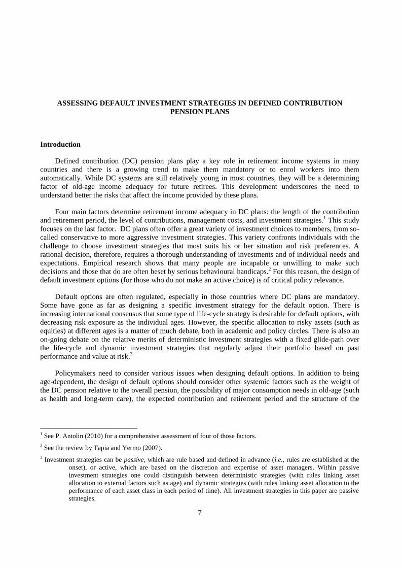
The investment strategies for each payout option are examined in the charts below, with the median
replacement rate (measure of return) on the y-axis, and the level of risk (replacement rates below the level
shown occur with a 5% probability) on the x-axis. As a result, all investment strategies lie around an
―efficient frontier‖, showing the trade-off between return and associated risk. The risk-return plot for the
case of the life annuity is shown in Figure 1. Figure 3 shows the results of the simulation for the case of the
variable programmed withdrawal, while Figure 4 shows the result of combined arrangements. The results
for the inflation-indexed life annuity and the fixed programmed withdrawal are not shown because they are
not substantially different from the others.16
The analysis below seeks to identify those strategies that
perform best and dominate others in the sense that they provide a higher median replacement rate for a
given risk level (or conversely, a lower risk level for a given median replacement rate).
Independently of the payout option, the analysis shows that an all-bond strategy and most strategies
with very low equity allocations (less than 20%) are seemingly inferior in the sense that there is always an
investment strategy that provides a higher return (median replacement rate) for a lower risk (higher
replacement rate at the 5th percentile).
17 However, the concentration of replacement rates below the 5
th risk
level is also highest for these strategies (Figure 2). Indeed, while not considered, a strategy of investing
exclusively in inflation-indexed bonds of the right maturity would deliver the closest to a riskless benefit,
in the sense that the replacement rate would not be affected by fluctuations in asset prices and inflation
during the accumulation stage. For very risk adverse individuals, such a strategy may be optimal.
15
The standard deviation and the median could be similar for a distribution having all points concentrated around the
mean and a few large outliers and a distribution with less concentration around the mean but less large
outliers. However, the first distribution will have a higher concentration than the second one.
16 See Scheuenstuhl et al. (2010) for the different graphs for all the different payout phases.
17 The all bond strategy is actually a portfolio with 5% in cash, 22.5% in government bonds and 72.5% in inflation-
linked bonds.
15
Figure 1. Life annuity: Median replacement rate vs. 5th percentile
1
2
3
4
5
6
7
8
9
10
11
12
13
14
15
16
17
18
1924
20
21
22
23
45
50
55
60
65
70
Me
dia
n R
R (
in %
)
26283032343638
Replacement rate at the 5th percentile (in %)
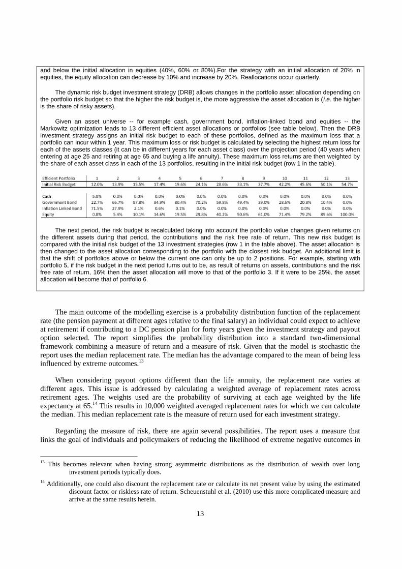
Note: Fixed portfolio with 0% in equities (1), 20% (2), 50% (3), and 80% (4); linear decrease life cycle with an initial exposure to equities of 20% (5), 50% (6), and 80% (7); step-wise function with an initial exposure to equities of 25% (8), 42.5% (9), 60%
(10), and 80% (11); x piece-wise linear function with an equity exposure of 20% (12), 50% (13), 80% (14), 90% (15); average multi-shaped function with an equity exposure of 20% (16), 50% (17), 80% (18), and 100% (19); the dynamic risk budget strategy
with an starting equity exposure of 20% (20), 40% (21), 60% (22), and 80% (23); and + the dynamic multi-shaped (24).
The relative performance of investment strategies depends on the form that the payout phase takes.
When the payout phase is either a life annuity or an inflation-indexed life annuity, life cycle strategies
provide a good trade-off between return and risk. Focusing on figures 1 and 2, corresponding to the life
annuity payout option, life cycle strategies based on the stepwise and the piecewise linear approaches, as
well as the average multi-shaped approach, show a higher median replacement rate for a relatively higher
replacement rate at the 5th percentile. Figure 1 shows that linear decrease life cycle strategies are always
dominated by stepwise strategies. Differences in performance are of the order of 1-3 percentage points in
the risk-adjusted replacement rate. For example, the difference in the median replacement rate between two
investment strategies with the same average time-weighted exposure to equities over the accumulation
period (40%) is 1.1 percentage points.18
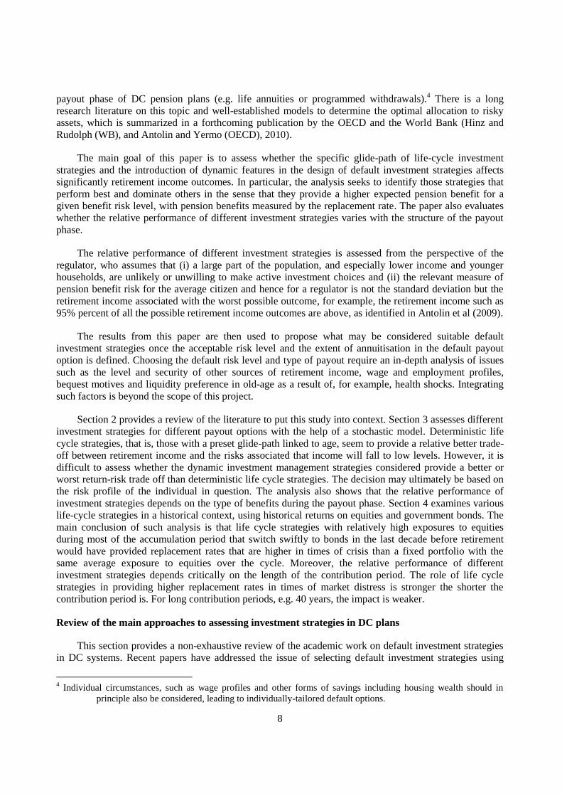
The dynamic multi-shaped strategy seems to offer a much higher
median replacement rate at the cost of a relatively small reduction in the replacement rate at the 5th
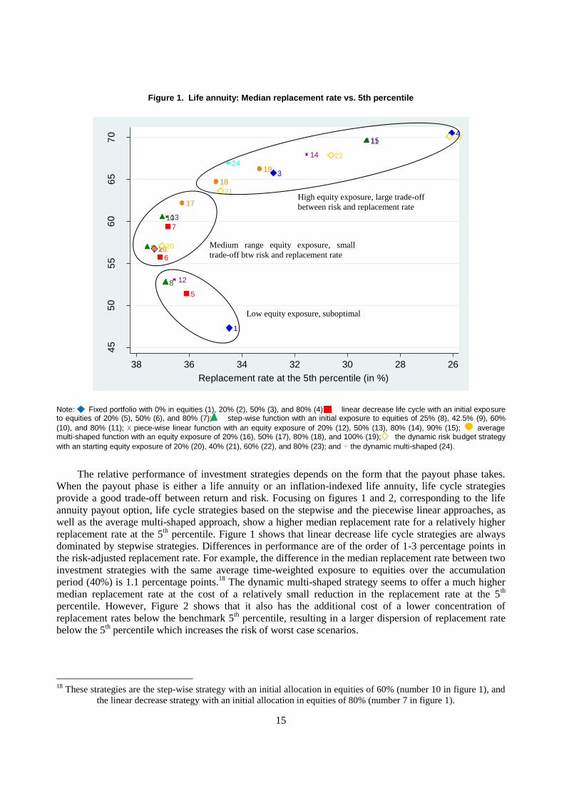
percentile. However, Figure 2 shows that it also has the additional cost of a lower concentration of
replacement rates below the benchmark 5th percentile, resulting in a larger dispersion of replacement rate
below the 5th percentile which increases the risk of worst case scenarios.
18
These strategies are the step-wise strategy with an initial allocation in equities of 60% (number 10 in figure 1), and
the linear decrease strategy with an initial allocation in equities of 80% (number 7 in figure 1).
Low equity exposure, suboptimal
Medium range equity exposure, small
trade-off btw risk and replacement rate
High equity exposure, large trade-off
between risk and replacement rate
16
Figure 2. Life annuity: Median replacement rate versus concentration below the 5th
percentile replacement rate
1
2
3
4
5
6
7
8
9
10
11
12
13
14
15
16
17
18
1924
20
21
22
23
45
50
55
60
65
70
Med
ian R
R (
in %
)
5060708090100Concentration of RRs below the 5th pctl (Probability in %)
Note: Fixed portfolio with 0% in equities (1), 20% (2), 50% (3), and 80% (4); linear decrease life cycle with an initial exposure to equities of 20% (5), 50% (6), and 80% (7); step-wise function with an initial exposure to equities of 25% (8), 42.5% (9), 60%
(10), and 80% (11); x piece-wise linear function with an equity exposure of 20% (12), 50% (13), 80% (14), 90% (15); average multi-shaped function with an equity exposure of 20% (16), 50% (17), 80% (18), and 100% (19); the dynamic risk budget strategy
with an starting equity exposure of 20% (20), 40% (21), 60% (22), and 80% (23); and + the dynamic multi-shaped (24).
Note: The concentration measure used is the probability that all those replacement rates that are below the replacement rate at the 5th
percentile are within a shortfall of 5 percentage points.
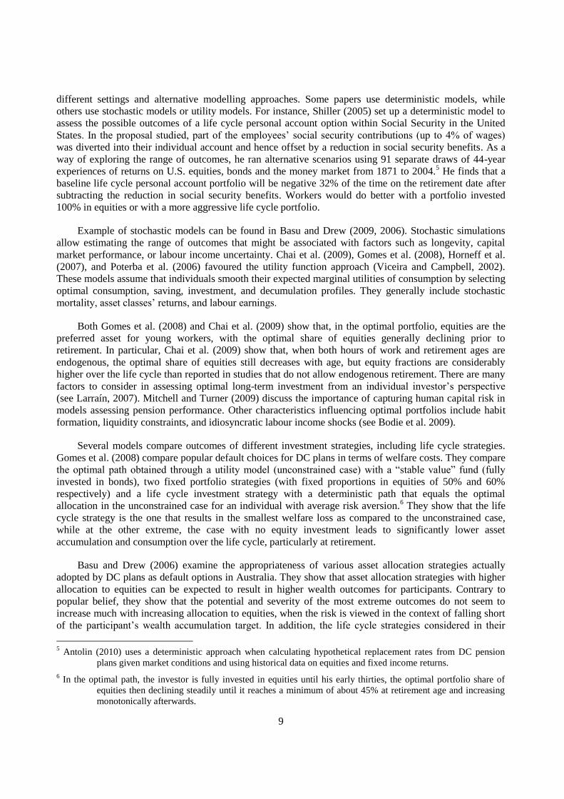
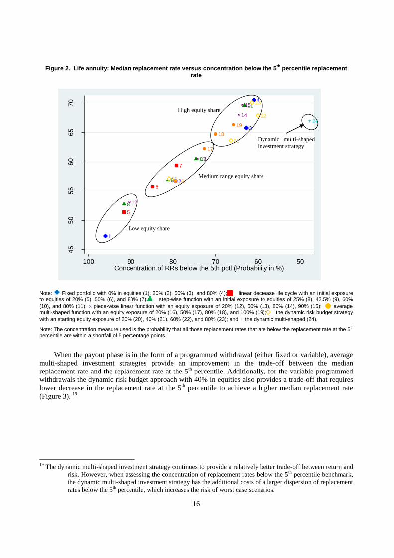
When the payout phase is in the form of a programmed withdrawal (either fixed or variable), average
multi-shaped investment strategies provide an improvement in the trade-off between the median
replacement rate and the replacement rate at the 5th percentile. Additionally, for the variable programmed
withdrawals the dynamic risk budget approach with 40% in equities also provides a trade-off that requires
lower decrease in the replacement rate at the 5th percentile to achieve a higher median replacement rate
(Figure 3). 19
19
The dynamic multi-shaped investment strategy continues to provide a relatively better trade-off between return and
risk. However, when assessing the concentration of replacement rates below the 5th
percentile benchmark,
the dynamic multi-shaped investment strategy has the additional costs of a larger dispersion of replacement
rates below the 5th
percentile, which increases the risk of worst case scenarios.
Low equity share
Medium range equity share
High equity share
Dynamic multi-shaped
investment strategy
17
Figure 3. Variable Programmed withdrawal: median replacement rate versus the replacement rate at the 5th percentile
1
2
3
4
5
6
7
8
9
10
11
12
13
14
15
16
17
18
1924
20
21
22
23
30
40
50
60
70
Me
dia
n R
R (
in %
)
202224262830
Replacement rate at the 5th percentile (in %)
Note: Fixed portfolio with 0% in equities (1), 20% (2), 50% (3), and 80% (4); linear decrease life cycle with an initial exposure to equities of 20% (5), 50% (6), and 80% (7); step-wise function with an initial exposure to equities of 25% (8), 42.5% (9), 60%
(10), and 80% (11); x piece-wise linear function with an equity exposure of 20% (12), 50% (13), 80% (14), 90% (15); average multi-shaped function with an equity exposure of 20% (16), 50% (17), 80% (18), and 100% (19); the dynamic risk budget strategy
with an starting equity exposure of 20% (20), 40% (21), 60% (22), and 80% (23); and + the dynamic multi-shaped (24).
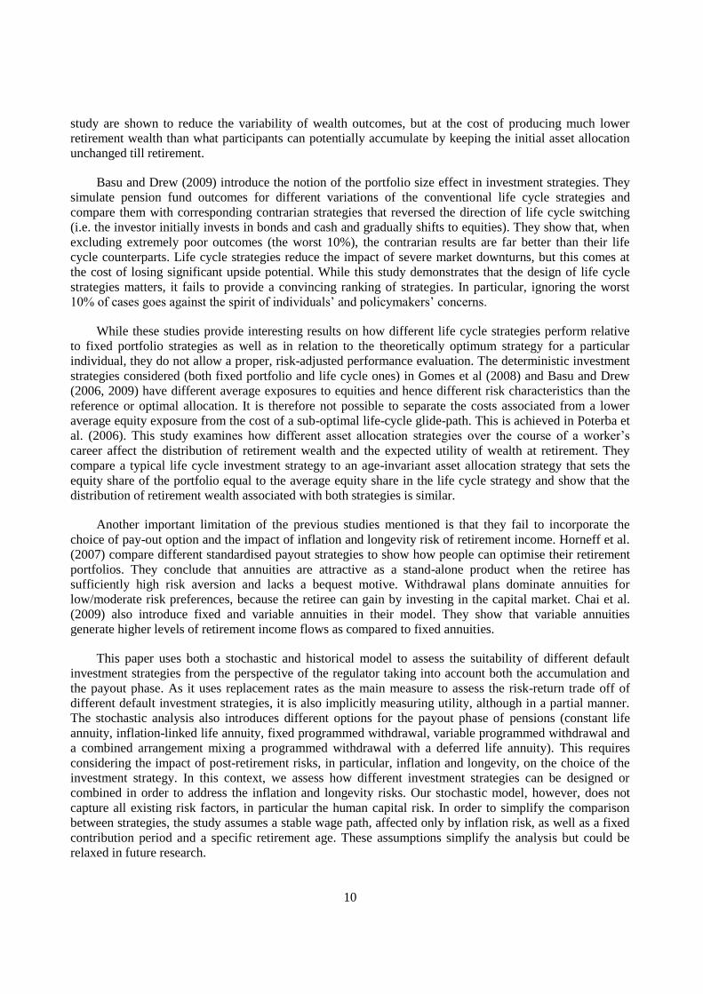
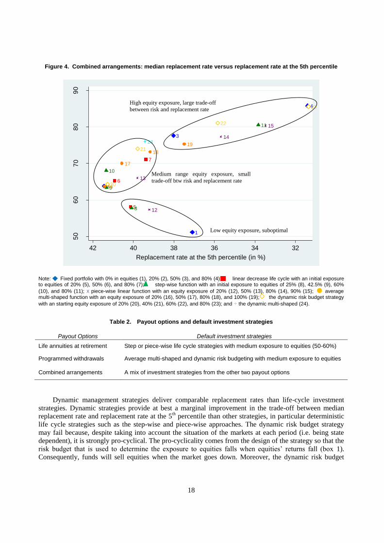
The investment strategies that perform relatively better when having combined payout arrangements
are a combination of those chosen for life annuity and programmed withdrawals payout options: the
stepwise linear approach starting with 60% in equities (number 10 in figure 4 below),20
the average multi-
shaped with 50% equities (number 17 in figure 4 below), and the dynamic risk budget with 40% in equities
(number 21 in figure 4 below). Table 2 summarises the default investment strategies given the type of
payout option.
20
The piecewise life cycle approach, which performs relatively well with life annuity, performs quite badly with
programmed withdrawals.
High equity exposure, large trade-off
between risk and replacement rate
Medium range equity exposure, small
trade-off btw risk and replacement rate
Low equity exposure, suboptimal
18
Figure 4. Combined arrangements: median replacement rate versus replacement rate at the 5th percentile
1
2
3
4
5
6
7
8
9
10
11
12
13
14
15
16
17
18
1924
20
21
22
23
50
60
70
80
90
Me
dia
n R
R (
in %
)
323436384042
Replacement rate at the 5th percentile (in %)
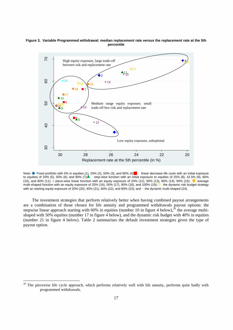
Note: Fixed portfolio with 0% in equities (1), 20% (2), 50% (3), and 80% (4); linear decrease life cycle with an initial exposure to equities of 20% (5), 50% (6), and 80% (7); step-wise function with an initial exposure to equities of 25% (8), 42.5% (9), 60%
(10), and 80% (11); x piece-wise linear function with an equity exposure of 20% (12), 50% (13), 80% (14), 90% (15); average multi-shaped function with an equity exposure of 20% (16), 50% (17), 80% (18), and 100% (19); the dynamic risk budget strategy
with an starting equity exposure of 20% (20), 40% (21), 60% (22), and 80% (23); and + the dynamic multi-shaped (24).
Table 2. Payout options and default investment strategies
Payout Options Default investment strategies
Life annuities at retirement Step or piece-wise life cycle strategies with medium exposure to equities (50-60%)
Programmed withdrawals Average multi-shaped and dynamic risk budgeting with medium exposure to equities
Combined arrangements A mix of investment strategies from the other two payout options
Dynamic management strategies deliver comparable replacement rates than life-cycle investment
strategies. Dynamic strategies provide at best a marginal improvement in the trade-off between median
replacement rate and replacement rate at the 5th percentile than other strategies, in particular deterministic
life cycle strategies such as the step-wise and piece-wise approaches. The dynamic risk budget strategy
may fail because, despite taking into account the situation of the markets at each period (i.e. being state
dependent), it is strongly pro-cyclical. The pro-cyclicality comes from the design of the strategy so that the
risk budget that is used to determine the exposure to equities falls when equities’ returns fall (box 1).
Consequently, funds will sell equities when the market goes down. Moreover, the dynamic risk budget
Low equity exposure, suboptimal
Medium range equity exposure, small
trade-off btw risk and replacement rate
High equity exposure, large trade-off
between risk and replacement rate
19
approach also suffers from short-termism as it focuses on a short-term risk measure.21
The dynamic multi-
shaped strategy also offers attractive risk-return trade-offs (Figures 1, 3 and 4), but fails to provide high
concentration below the 5th percentile (Figure 2). Consequently, there are more scenarios with replacement
rates lower than 5 percentage points below the 5th percentile under this strategy than under other strategies.
Finally, these dynamic strategies may perform alright in certain situations like 2008, but on average they
do not seem to provide much added value relative to life-cycle strategies.
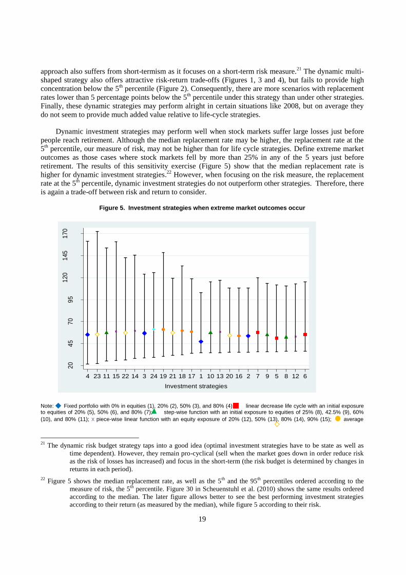
Dynamic investment strategies may perform well when stock markets suffer large losses just before
people reach retirement. Although the median replacement rate may be higher, the replacement rate at the
5th percentile, our measure of risk, may not be higher than for life cycle strategies. Define extreme market
outcomes as those cases where stock markets fell by more than 25% in any of the 5 years just before
retirement. The results of this sensitivity exercise (Figure 5) show that the median replacement rate is
higher for dynamic investment strategies.22
However, when focusing on the risk measure, the replacement
rate at the 5th percentile, dynamic investment strategies do not outperform other strategies. Therefore, there
is again a trade-off between risk and return to consider.
Figure 5. Investment strategies when extreme market outcomes occur
20
45
70
95
120
145
170
Rep
lace
me
nt ra
te (
in%
)
4 23 11 15 22 14 3 24 19 21 18 17 1 10 13 20 16 2 7 9 5 8 12 6
Investment strategies
Note: Fixed portfolio with 0% in equities (1), 20% (2), 50% (3), and 80% (4); linear decrease life cycle with an initial exposure to equities of 20% (5), 50% (6), and 80% (7); step-wise function with an initial exposure to equities of 25% (8), 42.5% (9), 60%
(10), and 80% (11); x piece-wise linear function with an equity exposure of 20% (12), 50% (13), 80% (14), 90% (15); average
21
The dynamic risk budget strategy taps into a good idea (optimal investment strategies have to be state as well as
time dependent). However, they remain pro-cyclical (sell when the market goes down in order reduce risk
as the risk of losses has increased) and focus in the short-term (the risk budget is determined by changes in
returns in each period).
22 Figure 5 shows the median replacement rate, as well as the 5
th and the 95
th percentiles ordered according to the
measure of risk, the 5th
percentile. Figure 30 in Scheuenstuhl et al. (2010) shows the same results ordered
according to the median. The later figure allows better to see the best performing investment strategies
according to their return (as measured by the median), while figure 5 according to their risk.
20
multi-shaped function with an equity exposure of 20% (16), 50% (17), 80% (18), and 100% (19); the dynamic risk budget strategy
with an starting equity exposure of 20% (20), 40% (21), 60% (22), and 80% (23); and + the dynamic multi-shaped (24).
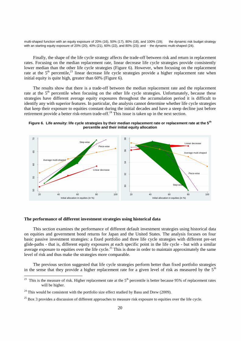
Finally, the shape of the life cycle strategy affects the trade-off between risk and return in replacement
rates. Focusing on the median replacement rate, linear decrease life cycle strategies provide consistently
lower median than the other life cycle strategies (Figure 6). However, when focusing on the replacement
rate at the 5th percentile,
23 linear decrease life cycle strategies provide a higher replacement rate when
initial equity is quite high, greater than 60% (Figure 6).
The results show that there is a trade-off between the median replacement rate and the replacement
rate at the 5th percentile when focusing on the other life cycle strategies. Unfortunately, because these
strategies have different average equity exposures throughout the accumulation period it is difficult to
identify any with superior features. In particular, the analysis cannot determine whether life cycle strategies
that keep their exposure to equities constant during the initial decades and have a steep decline just before
retirement provide a better risk-return trade-off.24
This issue is taken up in the next section.
Figure 6. Life annuity: life cycle strategies by their median replacement rate or replacement rate at the 5th
percentile and their initial equity allocation
Step-wise
Piece-wise
Average multi-shaped
Linear decrease
50
55
60
65
70
Me
dia
n R
R (
in %
)
20 40 60 80 100
Initial allocation in equities (in %)
Linear decrease
Average multi-shaped
Piece-wise
Step-wise
30
32
34
36
38
5th
perc
entile
(in
%)
20 40 60 80 100
Initial allocation in equities (in %)
The performance of different investment strategies using historical data
This section examines the performance of different default investment strategies using historical data
on equities and government bond returns for Japan and the United States. The analysis focuses on four
basic passive investment strategies: a fixed portfolio and three life cycle strategies with different pre-set
glide-paths - that is, different equity exposures at each specific point in the life cycle - but with a similar
average exposure to equities over the life cycle.25
This is done in order to maintain approximately the same
level of risk and thus make the strategies more comparable.
The previous section suggested that life cycle strategies perform better than fixed portfolio strategies
in the sense that they provide a higher replacement rate for a given level of risk as measured by the 5th
23
This is the measure of risk. Higher replacement rate at the 5th
percentile is better because 95% of replacement rates
will be higher.
24 This would be consistent with the portfolio size effect studied by Basu and Drew (2009).
25 Box 3 provides a discussion of different approaches to measure risk exposure to equities over the life cycle.
21
percentile. In addition, the previous section failed to provide a clear cut answer on which glide-path among
different life cycle strategies provided a higher median replacement rate for the same level of risk.
This section assesses whether, using historical data on returns from Japanese and US equities and
government bonds, life cycle investment strategies would have performed better than fixed portfolios, and
which life cycle strategy would have done best. This is done by calculating hypothetical replacement rates
for cohorts retiring from 1940 to 2008 that would have contributed continuously 5% of wages into a DC
pension plan over a 40-year period (from age 25 to age 65).26
The results are also compared with a 20-year
contribution period. At retirement, pensioners buy a life annuity given government bond yields at the time.
Consequently, the difference between each cohort’s hypothetical replacement rates is determined by
market conditions during the accumulation period and at the time of retirement.
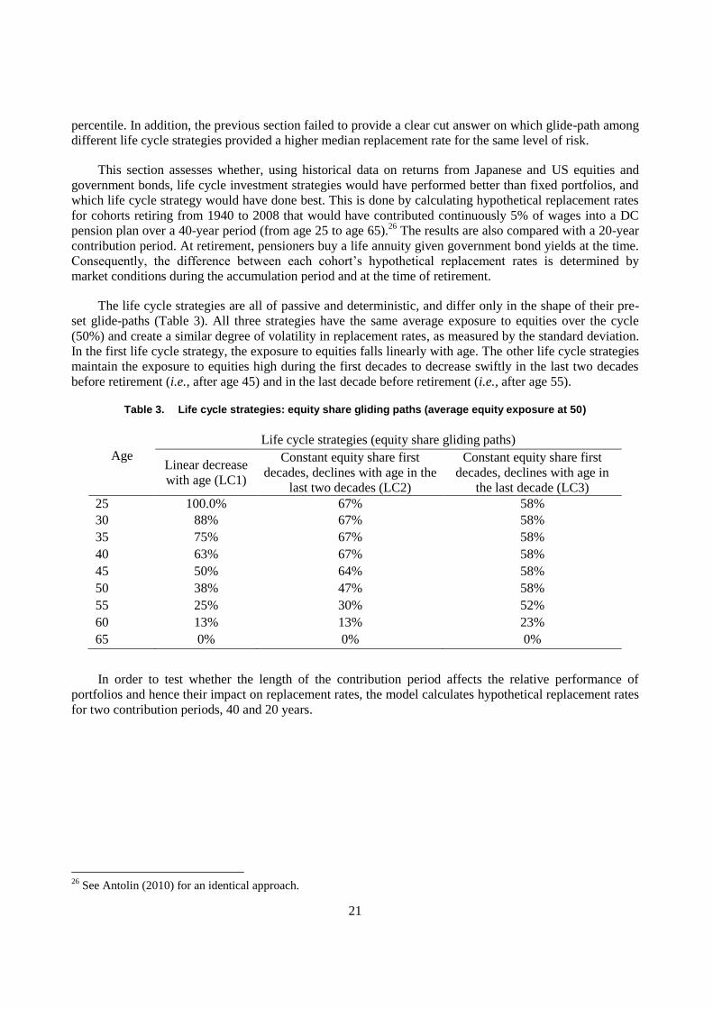
The life cycle strategies are all of passive and deterministic, and differ only in the shape of their pre-
set glide-paths (Table 3). All three strategies have the same average exposure to equities over the cycle
(50%) and create a similar degree of volatility in replacement rates, as measured by the standard deviation.
In the first life cycle strategy, the exposure to equities falls linearly with age. The other life cycle strategies
maintain the exposure to equities high during the first decades to decrease swiftly in the last two decades
before retirement (i.e., after age 45) and in the last decade before retirement (i.e., after age 55).
Table 3. Life cycle strategies: equity share gliding paths (average equity exposure at 50)
Age
Life cycle strategies (equity share gliding paths)
Linear decrease
with age (LC1)
Constant equity share first
decades, declines with age in the
last two decades (LC2)
Constant equity share first
decades, declines with age in
the last decade (LC3)
25 100.0% 67% 58%
30 88% 67% 58%
35 75% 67% 58%
40 63% 67% 58%
45 50% 64% 58%
50 38% 47% 58%
55 25% 30% 52%
60 13% 13% 23%
65 0% 0% 0%
In order to test whether the length of the contribution period affects the relative performance of
portfolios and hence their impact on replacement rates, the model calculates hypothetical replacement rates
for two contribution periods, 40 and 20 years.
26
See Antolin (2010) for an identical approach.
22
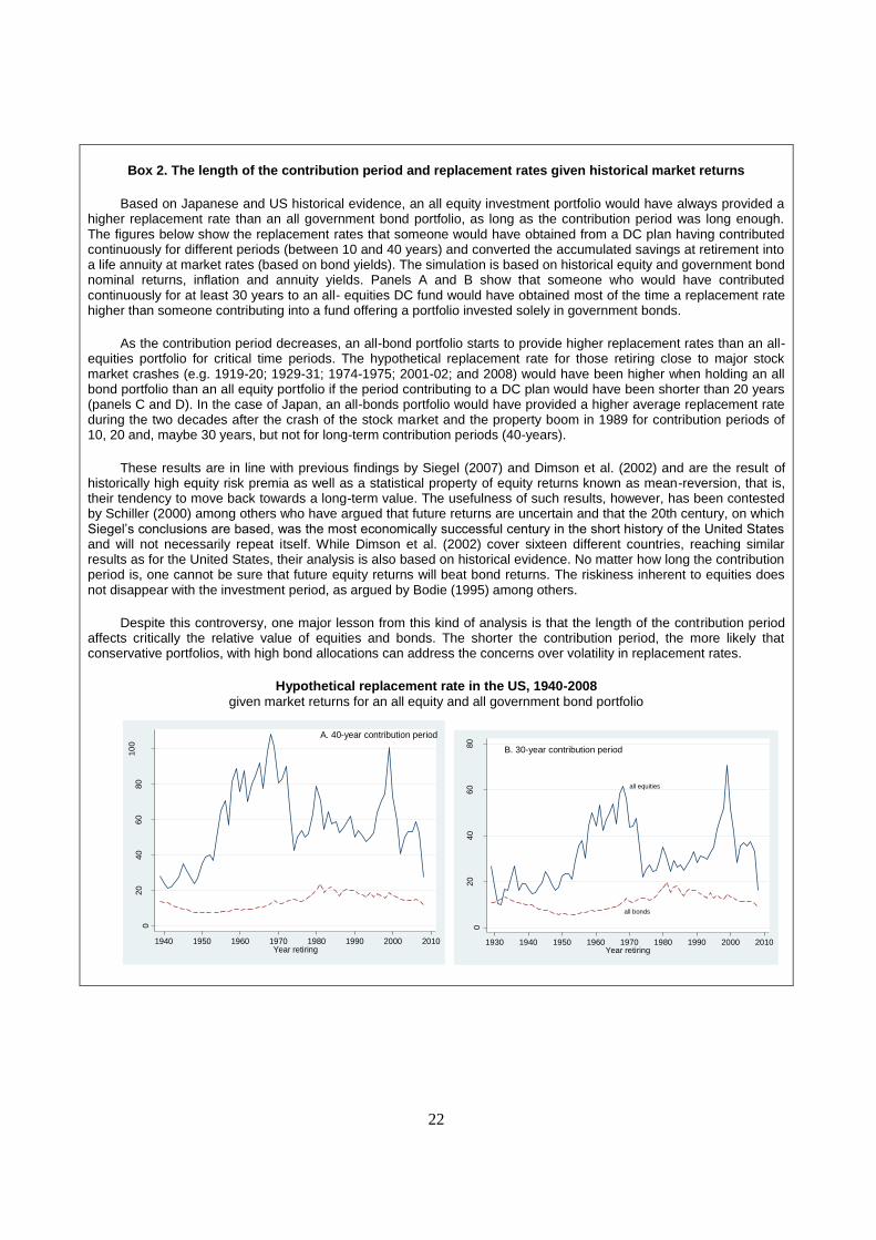
Box 2. The length of the contribution period and replacement rates given historical market returns
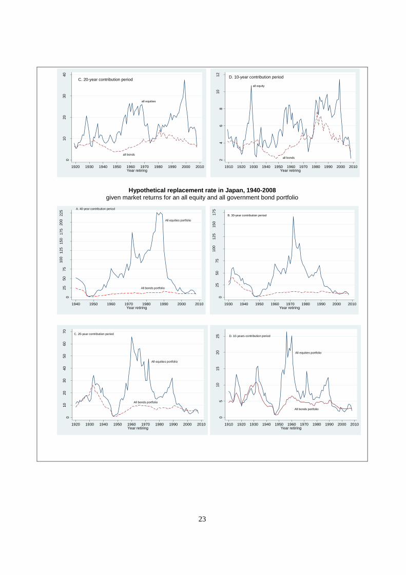
Based on Japanese and US historical evidence, an all equity investment portfolio would have always provided a higher replacement rate than an all government bond portfolio, as long as the contribution period was long enough. The figures below show the replacement rates that someone would have obtained from a DC plan having contributed continuously for different periods (between 10 and 40 years) and converted the accumulated savings at retirement into a life annuity at market rates (based on bond yields). The simulation is based on historical equity and government bond nominal returns, inflation and annuity yields. Panels A and B show that someone who would have contributed continuously for at least 30 years to an all- equities DC fund would have obtained most of the time a replacement rate higher than someone contributing into a fund offering a portfolio invested solely in government bonds.
As the contribution period decreases, an all-bond portfolio starts to provide higher replacement rates than an all-equities portfolio for critical time periods. The hypothetical replacement rate for those retiring close to major stock market crashes (e.g. 1919-20; 1929-31; 1974-1975; 2001-02; and 2008) would have been higher when holding an all bond portfolio than an all equity portfolio if the period contributing to a DC plan would have been shorter than 20 years (panels C and D). In the case of Japan, an all-bonds portfolio would have provided a higher average replacement rate during the two decades after the crash of the stock market and the property boom in 1989 for contribution periods of 10, 20 and, maybe 30 years, but not for long-term contribution periods (40-years).
These results are in line with previous findings by Siegel (2007) and Dimson et al. (2002) and are the result of historically high equity risk premia as well as a statistical property of equity returns known as mean-reversion, that is, their tendency to move back towards a long-term value. The usefulness of such results, however, has been contested by Schiller (2000) among others who have argued that future returns are uncertain and that the 20th century, on which Siegel’s conclusions are based, was the most economically successful century in the short history of the United States and will not necessarily repeat itself. While Dimson et al. (2002) cover sixteen different countries, reaching similar results as for the United States, their analysis is also based on historical evidence. No matter how long the contribution period is, one cannot be sure that future equity returns will beat bond returns. The riskiness inherent to equities does not disappear with the investment period, as argued by Bodie (1995) among others.
Despite this controversy, one major lesson from this kind of analysis is that the length of the contribution period affects critically the relative value of equities and bonds. The shorter the contribution period, the more likely that conservative portfolios, with high bond allocations can address the concerns over volatility in replacement rates.
Hypothetical replacement rate in the US, 1940-2008
given market returns for an all equity and all government bond portfolio
A. 40-year contribution period
020
40
60
80
10
0
retire
men
t in
com
e o
verf
inal sa
lary
(%
)
1940 1950 1960 1970 1980 1990 2000 2010Year retiring
all equities
all bonds
B. 30-year contribution period
020
40
60
80
retire
men
t in
com
e o
verf
inal sa
lary
(%
)
1930 1940 1950 1960 1970 1980 1990 2000 2010Year retiring
23
all equities
all bonds
C. 20-year contribution period
010
20
30
40
retire
men
t in
com
e o
verf
inal sa
lary
(%
)
1920 1930 1940 1950 1960 1970 1980 1990 2000 2010Year retiring
all equity
all bonds
D. 10-year contribution period
24
68
10
12
retire
men
t in
com
e o
verf
inal sa
lary
(%
)
1910 1920 1930 1940 1950 1960 1970 1980 1990 2000 2010Year retiring
Hypothetical replacement rate in Japan, 1940-2008
given market returns for an all equity and all government bond portfolio
All equities portfolio
All bonds portfolio
A. 40-year contribution period
025
50
75
10
012
515
017
520
022
5
retire
men
t in
com
e o
ver
fina
l sala
ry (
%)
1940 1950 1960 1970 1980 1990 2000 2010Year retiring
B. 30-year contribution period
025
50
75
10
012
515
017
5
retire
men
t in
com
e o
ver
fina
l sala
ry (
%)
1930 1940 1950 1960 1970 1980 1990 2000 2010Year retiring
All equities portfolio
All bonds portfolio
C. 20-year contribution period
010
20
30
40
50
60
70
retire
men
t in
com
e o
ver
fina
l sala
ry (
%)
1920 1930 1940 1950 1960 1970 1980 1990 2000 2010Year retiring
All equities portfolio
All bonds portfolio
D. 10-years contribution period
05
10
15
20
25
retire
men
t in
com
e o
ver
fina
l sala
ry (
%)
1910 1920 1930 1940 1950 1960 1970 1980 1990 2000 2010Year retiring
24
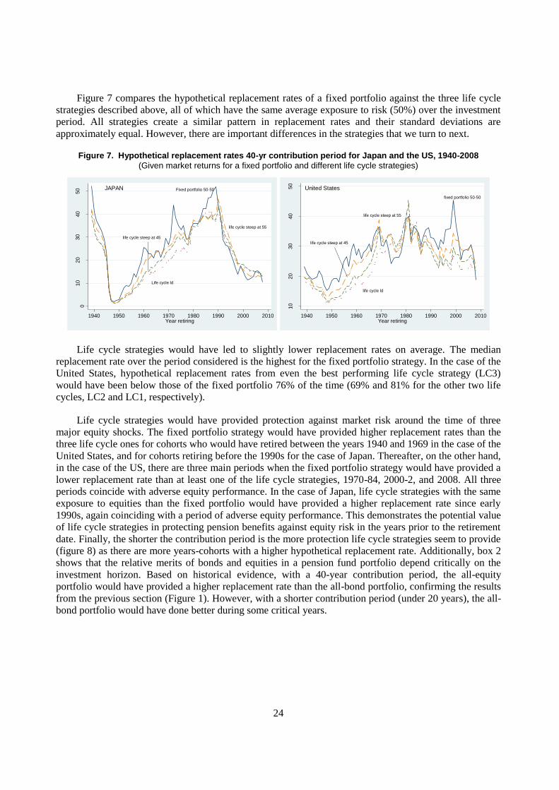
Figure 7 compares the hypothetical replacement rates of a fixed portfolio against the three life cycle
strategies described above, all of which have the same average exposure to risk (50%) over the investment
period. All strategies create a similar pattern in replacement rates and their standard deviations are
approximately equal. However, there are important differences in the strategies that we turn to next.
Figure 7. Hypothetical replacement rates 40-yr contribution period for Japan and the US, 1940-2008
(Given market returns for a fixed portfolio and different life cycle strategies)
Fixed portfolio 50-50
Life cycle ld
life cycle steep at 55
life cycle steep at 45
JAPAN
010
20
30
40
50
retire
men
t in
co
me o
ve
r fin
al sa
lary
(%
)
1940 1950 1960 1970 1980 1990 2000 2010Year retiring
fixed portfolio 50-50
life cycle steep at 55
life cycle ld
life cycle steep at 45
United States
10
20
30
40
50
retire
men
t in
co
me o
ve
r fin
al sa
lary
(%
)
1940 1950 1960 1970 1980 1990 2000 2010Year retiring
Life cycle strategies would have led to slightly lower replacement rates on average. The median
replacement rate over the period considered is the highest for the fixed portfolio strategy. In the case of the
United States, hypothetical replacement rates from even the best performing life cycle strategy (LC3)
would have been below those of the fixed portfolio 76% of the time (69% and 81% for the other two life
cycles, LC2 and LC1, respectively).
Life cycle strategies would have provided protection against market risk around the time of three
major equity shocks. The fixed portfolio strategy would have provided higher replacement rates than the
three life cycle ones for cohorts who would have retired between the years 1940 and 1969 in the case of the
United States, and for cohorts retiring before the 1990s for the case of Japan. Thereafter, on the other hand,
in the case of the US, there are three main periods when the fixed portfolio strategy would have provided a
lower replacement rate than at least one of the life cycle strategies, 1970-84, 2000-2, and 2008. All three
periods coincide with adverse equity performance. In the case of Japan, life cycle strategies with the same
exposure to equities than the fixed portfolio would have provided a higher replacement rate since early
1990s, again coinciding with a period of adverse equity performance. This demonstrates the potential value
of life cycle strategies in protecting pension benefits against equity risk in the years prior to the retirement
date. Finally, the shorter the contribution period is the more protection life cycle strategies seem to provide
(figure 8) as there are more years-cohorts with a higher hypothetical replacement rate. Additionally, box 2
shows that the relative merits of bonds and equities in a pension fund portfolio depend critically on the
investment horizon. Based on historical evidence, with a 40-year contribution period, the all-equity
portfolio would have provided a higher replacement rate than the all-bond portfolio, confirming the results
from the previous section (Figure 1). However, with a shorter contribution period (under 20 years), the all-
bond portfolio would have done better during some critical years.
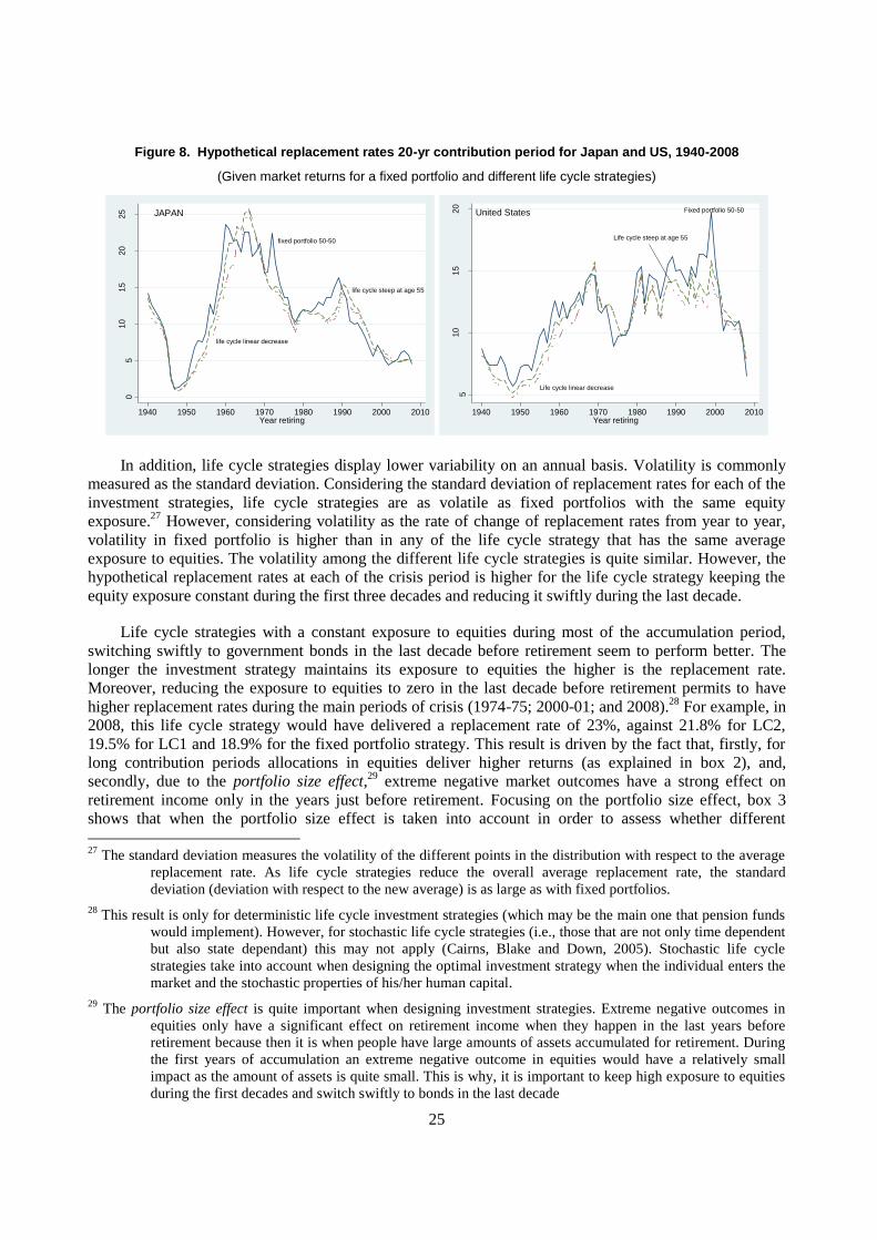
25
Figure 8. Hypothetical replacement rates 20-yr contribution period for Japan and US, 1940-2008
(Given market returns for a fixed portfolio and different life cycle strategies)
fixed portfolio 50-50
life cycle steep at age 55
life cycle linear decrease
05
10
15
20
25
retire
men
t in
com
e o
ver
fina
l sala
ry (
%)
1940 1950 1960 1970 1980 1990 2000 2010Year retiring
JAPAN Fixed portfolio 50-50
Life cycle linear decrease
Life cycle steep at age 55
United States
510
15
20
retire
men
t in
com
e o
ver
fina
l sala
ry (
%)
1940 1950 1960 1970 1980 1990 2000 2010Year retiring
In addition, life cycle strategies display lower variability on an annual basis. Volatility is commonly
measured as the standard deviation. Considering the standard deviation of replacement rates for each of the
investment strategies, life cycle strategies are as volatile as fixed portfolios with the same equity
exposure.27
However, considering volatility as the rate of change of replacement rates from year to year,
volatility in fixed portfolio is higher than in any of the life cycle strategy that has the same average
exposure to equities. The volatility among the different life cycle strategies is quite similar. However, the
hypothetical replacement rates at each of the crisis period is higher for the life cycle strategy keeping the
equity exposure constant during the first three decades and reducing it swiftly during the last decade.
Life cycle strategies with a constant exposure to equities during most of the accumulation period,
switching swiftly to government bonds in the last decade before retirement seem to perform better. The
longer the investment strategy maintains its exposure to equities the higher is the replacement rate.
Moreover, reducing the exposure to equities to zero in the last decade before retirement permits to have
higher replacement rates during the main periods of crisis (1974-75; 2000-01; and 2008).28
For example, in
2008, this life cycle strategy would have delivered a replacement rate of 23%, against 21.8% for LC2,
19.5% for LC1 and 18.9% for the fixed portfolio strategy. This result is driven by the fact that, firstly, for
long contribution periods allocations in equities deliver higher returns (as explained in box 2), and,
secondly, due to the portfolio size effect,29
extreme negative market outcomes have a strong effect on
retirement income only in the years just before retirement. Focusing on the portfolio size effect, box 3
shows that when the portfolio size effect is taken into account in order to assess whether different
27
The standard deviation measures the volatility of the different points in the distribution with respect to the average
replacement rate. As life cycle strategies reduce the overall average replacement rate, the standard
deviation (deviation with respect to the new average) is as large as with fixed portfolios.
28 This result is only for deterministic life cycle investment strategies (which may be the main one that pension funds
would implement). However, for stochastic life cycle strategies (i.e., those that are not only time dependent
but also state dependant) this may not apply (Cairns, Blake and Down, 2005). Stochastic life cycle
strategies take into account when designing the optimal investment strategy when the individual enters the
market and the stochastic properties of his/her human capital.
29 The portfolio size effect is quite important when designing investment strategies. Extreme negative outcomes in
equities only have a significant effect on retirement income when they happen in the last years before
retirement because then it is when people have large amounts of assets accumulated for retirement. During
the first years of accumulation an extreme negative outcome in equities would have a relatively small
impact as the amount of assets is quite small. This is why, it is important to keep high exposure to equities
during the first decades and switch swiftly to bonds in the last decade

26
investment strategies have the same risk exposure to equities, life cycle strategies would have a higher
equity allocation in the initial years of the accumulation with respect to the allocation used in the analysis
of this section (Table 2). Consequently, taking into account the portfolio size effect to determine the risk
exposure to equities will lead to comparable life cycle strategies with higher replacement rates, reinforcing
the positive effect of life cycle strategies described in this section.
Box 3. Comparing investment strategies
The analysis of the performance of different investment strategies needs to take into account their different exposures to risk. Therefore, any comparison of performance is only meaningful when comparing investment strategies with the same overall risk exposure. The investment strategies examined in this paper are defined by their allocation to equities and bonds. These allocations can be constant or vary over time. Consequently, in the case of two investment strategies that have different equity allocation at different points in time in the life-cycle, there is a need for a measure to determine whether they have the same overall equity exposure or not.
There are different approaches to measure the overall risk exposure to equities (risk exposure) of different investment strategies over time. The simplest approach is to measure the overall equity exposure by calculating the average exposure to equities over the life cycle. That is, the average exposure to equities of an investment strategy is the sum of the equity allocation of the portfolio in each period divided by the length of the contribution period. This is the approach used in the section above.
However, this time-weighted measure of equity exposure fails to consider the impact of the growing asset base, the so-called portfolio size effect. The size of the portfolio determines the importance of the risk and impact of the exposure to equities. For example, at the beginning of the accumulation for retirement, the assets accumulated are relatively low while during the last years before retirement the assets accumulated can be quite large. Therefore, a strong negative or positive increase in equity returns will have a different effect in the final accumulation just before retirement depending on whether it occurs at the beginning or the end of the accumulation period. Consequently, a 30% exposure to equities has a different impact and different risk profile whether it is at the beginning or at the end of the accumulation period.
In order to account for the portfolio size effect one could calculate a money-weighted or volume-weighted average exposure to equities. This measure of the overall risk exposure to equities of different investment strategies would use the size of the assets accumulated at each period in the life cycle. Unfortunately, this can only be done a posteriori, once the entire accumulation process has run its course and the returns to the different assets comprising the portfolio at each point in time are known.
However, to compare the performance of investment strategies with a similar overall risk exposure to equities, the measure of risk exposure to equities needs to be defined a priori. A priori the size or volume of the assets accumulated at each point in time are not known and, therefore, a volume weighted measure is not feasible.
Nevertheless, one could calculate a measure of the risk exposure to equities of different investment strategies taking into account the portfolio size effect by weighting the share of equities in the portfolio at each point in time of the accumulation period by the age of the individual. This measure reflects the idea that the older the individual gets the bigger the weight for equity exposure needs to be, reflecting the idea that the size or volume of the assets accumulated increases as people get closer to retirement. The measure could be enhanced by assuming a return on investment during the accumulation period as well as a fixed contribution over time. Table 3.1 below shows different measures of the overall risk exposure to equities for four different investment strategies. These four investment strategies have the same overall risk exposures to equities when using the time weighted measure, 50%. However, this is no longer the case when using any of the other three measures that account for the portfolio size effect. The measures approximating for the portfolio size effect suggest that life cycle strategies may have a lower overall exposure to risk than a fixed portfolio, and, within the life cycle strategies, the linear decrease with respect to age may have the lowest overall exposure to equities.
These three measures that try to approximate the impact of the portfolio size effect require several assumptions, in particular as regard returns on investment over the life cycle. Obviously, these assumptions are arbitrary. This is the reason to use in the analysis of the current section the time weighted average measure of overall risk exposure.
Table 3.1. Risk exposure to equities of different investment strategies
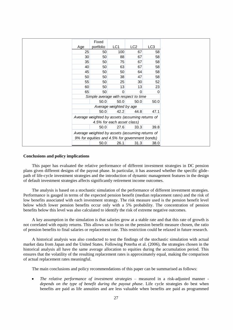
27
Age
Fixed
portfolio LC1 LC2 LC3
25 50 100 67 58
30 50 88 67 58
35 50 75 67 58
40 50 63 67 58
45 50 50 64 58
50 50 38 47 58
55 50 25 30 52
60 50 13 13 23
65 50 0 0 0
50.0 50.0 50.0 50.0
50.0 42.2 44.8 47.1
50.0 27.6 33.3 39.8
50.0 26.1 31.3 38.0
Simple average with respect to time
Average weighted by assets (assuming returns of
4.5% for each asset class)
Average weighted by age
Average weighted by assets (assuming returns of
9% for equities and 4.5% for government bonds)
Conclusions and policy implications
This paper has evaluated the relative performance of different investment strategies in DC pension
plans given different designs of the payout phase. In particular, it has assessed whether the specific glide-
path of life-cycle investment strategies and the introduction of dynamic management features in the design
of default investment strategies affects significantly retirement income outcomes.
The analysis is based on a stochastic simulation of the performance of different investment strategies.
Performance is gauged in terms of the expected pension benefit (median replacement rates) and the risk of
low benefits associated with each investment strategy. The risk measure used is the pension benefit level
below which lower pension benefits occur only with a 5% probability. The concentration of pension
benefits below this level was also calculated to identify the risk of extreme negative outcomes.
A key assumption in the simulation is that salaries grow at a stable rate and that this rate of growth is
not correlated with equity returns. This allows us to focus on the pension benefit measure chosen, the ratio
of pension benefits to final salaries or replacement rate. This restriction could be relaxed in future research.
A historical analysis was also conducted to test the findings of the stochastic simulation with actual
market data from Japan and the United States. Following Poterba et al. (2006), the strategies chosen in the
historical analysis all have the same average allocation to equities during the accumulation period. This
ensures that the volatility of the resulting replacement rates is approximately equal, making the comparison
of actual replacement rates meaningful.
The main conclusions and policy recommendations of this paper can be summarised as follows:
The relative performance of investment strategies – measured in a risk-adjusted manner -
depends on the type of benefit during the payout phase. Life cycle strategies do best when
benefits are paid as life annuities and are less valuable when benefits are paid as programmed
28
withdrawals. Dynamic strategies seem to work better with programmed withdrawals. A mixed of
life-cycle and dynamic strategies may be required when benefits are paid combining programmed
withdrawals and deferred life annuities bought at the time of retirement.
Life cycle strategies that maintain a constant exposure to equities during most of the
accumulation period, switching swiftly to bonds in the last decade before retirement seem to
perform best. The historical analysis confirms that the value of such strategies stems from the
protection of pension benefits from major market shocks in the years preceding retirement. These
results confirm the importance of the portfolio size effect identified by Basu and Drew (2009).
The introduction of dynamic investment management strategies can provide somewhat higher
replacement rates for a given level of risk than the more deterministic or pre-set strategies, at
least in the case of pay-outs in the form of variable withdrawals. However, their pro-cyclicality
may affect their performance. They tend to sell equities when prices fall and buy them when
prices go up, missing in the cumulative return of good times. Further research on such strategies
is necessary, as some of the ones considered suffer from a pro-cyclical bias. It is possible that a
dynamic strategy that considers the long-term evolution of the equity premium and the nature of
mean-reversion in equity returns could capture some gains for pension plan members as it has
been suggested by Viceira (2009) and Martellini (2009) among others.
The length of the contribution period affects the ranking of the different investment strategies.
The historical analysis shows that life cycle strategies perform better than fixed portfolios when
the contribution period is only 20 instead of 40 years. Longer contribution periods reduce the
implicit attractiveness of life cycle strategies (as the higher replacement rates obtained in crisis
periods are offset by lower rates in boom times). For short contribution periods, life cycle
strategies and the type of gliding path become more relevant to assure higher replacement rate
outcomes in crisis periods. These results call for further investigation of the impact of the
contribution period on pension benefits and the choice of investment strategy, as in Gomes et al.
(2008).
The analysis in this paper also highlights other more technical factors to consider when designing
default investment strategies. Firstly, the difference between the best and worst performing strategies is
substantial, of the order of 1-3 percentage points in replacement rates. When accumulated over a typical
retirement period of twenty years, this implies a cumulative loss of benefits of between one third and 100%
of the final salary prior to retirement. Secondly, it is the level of the average allocation to equities over the
investment period rather than the specific design of the glide-path what drives the level and volatility of
replacement rates. This result stresses the importance of modelling based on individual utility or welfare
functions that take into account risk aversion, human capital, as well as other sources of retirement income.
Through such models, plan sponsors, providers and policymakers can identify optimal asset allocations for
representative individuals and hence design suitable default investment strategies with specific weights for
each asset class. And finally, this study has highlighted the value of both stochastic and historical analysis
to understand better the value of different investment strategies. While the strategic asset allocation, that is,
the average allocation to different asset classes during the accumulation period, is the main determinant of
the level and volatility of pension benefits, well-designed life cycle strategies can help protect pension
benefits from extreme negative outcomes without jeopardising high replacement rates for the average
generation.
29
REFERENCES
Antolín, P. (2010), ―Private Pensions and the Financial Crisis: How to ensure adequate retirement income
from defined contribution pension plans?‖ Financial Market Trends, Vol. 2009, No. 2.
Antolín, P., S. Blome, D. Karim, S. Payet, G. Scheuenstuhl, and J. Yermo (2009), ―Investment Regulations
and Defined Contribution Pensions?‖ Working Paper in Insurance and Private Pensions, No. 39
asu, A., Drew, M. (2006), Appropriateness of Default Investment Options in Defined Contribution Plans:
The Australian Evidence, MPRA Paper No. 3314.
Basu, A.K., Drew, M.E. (2009), Portfolio Size Effect in Retirement Accounts: What Does It Imply for
Lifecycle Asset Allocation Funds?, The Journal of Portfolio Management.
Bodie, Z. (1995), On the Risk of Stocks in the Long Run, Financial Analysts Journal, May/June 1995.
Bodie, Z., Detemple, J., Rindisbacher, M. (2009), Life cycle Finance and the Design of Pension Plans,
Boston University School of Management Research Paper Series, No. 2009-5.
Cairns, A.J.G, D. Blake and K. Down (2006), ―Stochastic lifestyling: Optimal dynamic asset allocation for
defined contribution pension plans‖, Journal of Economic Dynamics and Control, 30, 843-877
Campbell, J.Y. and Viceira, L.M. (2002), Strategic Asset Allocation: Portfolio Choice for Long-Term
Investors. Oxford University Press.
Chai, J., Horneff, W., Maurer, R., Mitchell, O.S. (2009), Extending Life Cycle Models of Optimal
Portfolio Choice Integrating Flexible Work, Endogenous Retirement, and Investment Decisions with
lifetime Payouts, NBER Working Paper Series, No 15079.
Dimson, E., Marsh, P. and & Staunton, M. (2002), Triumph of the Optimists:101 Years of Global
Investment Returns. Princeton.
Gomes, F.J., Kotlikoff, L.J., Viceira, L.M. (2008), Optimal Life cycle Investing with Flexible Labor
Supply: a Welfare Analysis of Life cycle Funds, NBER Working Paper Series, No. 13966.
Hinz and Rudolph (WB), and Antolin and Yermo (OECD), Eds. (2010), Evaluating the Financial
Performance of Pension Funds, The World Bank Publications, forthcoming.
Horneff, W.J., Maurer, R. H., Mitchell, O.S., Dus, I. (2007), Following the Rules: Integrating Asset
Allocation and Annuitization in Retirement Portfolios, Insurance: Mathematics and Economics. 42:
2007: 396-408.
Larraín, G. (2007), ―Portfolio Investment in an Intertemporal Setting: Assessment of the Literature and
Policy Implications for Latin American Pension Systems‖, OECD Working Papers on Insurance and
Private Pensions, No. 10, OECD, Paris.
30
Martellini, L. (2009), Guest Viewpoint - Target date: “There is ample room for added value between one
size-fits-all solutions and do-it-yourself approaches to long-term investment decisions”, IPE
Magazine, September 2009.
Mitchell, O.S., Turner, J.A. (2009), Labor Market uncertainty and Pension System Performance,
Performance of Privately Managed Pension Funds.
Mottola, G.R., Utkus, S.P. (2009), Red, Yellow, and Green: Measuring the Quality of 401(k) Portfolio
Choices, Chapter 4 in Overcoming the Saving Slump: How to Increase the Effectiveness of
Financial Education and Saving Programs, edited by Annamaria Lusardi, University of Chicago
Press.
Poterba, J., Rauh, J., Venti, S., Wise, D. (2006), Lifecycle Asset Allocation Strategies and the Distribution
of 401(k) Retirement Wealth, NBER Working Paper Series, No 11974.
Shiller, R.J. (2000), Irrational Exuberance, Princeton.
Shiller, R.J. (2005), The Life cycle Personal Accounts Proposal for Social Security: An Evaluation, NBER
Working Paper Series, No. 11300.
Siegel, J. J. (2007). Stocks for the Long Run: The Definitive Guide to Financial Market Returns and Long-
Term Investment Strategies (4th ed.). New York: McGraw-Hill.
Scheuenstuhl G., S. Blome, W. Mader, D. Karim, and T. Friederich (2010), ―Assessing Investment
Strategies in Defined Contribution Pension Plans under Various Payout Options‖, Risklab working
paper series under: http://www.risklab.com/de/meta/publikationen/index.html
Tapia, W. and Yermo, J. (2007), "Implications of Behavioural Economics for Mandatory Individual
Account Pension Systems", OECD Working Papers on Insurance and Private Pensions, No. 11, July
2007.
Viceira, L. (2009), "Life-Cycle Funds‖, forthcoming in Annamaria Lusardi, ed., Overcoming the saving
slump: How to increase the effectiveness of financial education and saving programs, University of
Chicago Press.