Embed Size (px)
Citation preview
PEMODELAN DAN PERAMALAN DATA
PEMBUKAAN IHSG MENGGUNAKAN
MODEL ARIMA
OLEH :OLEH :
1. Triyono ( M0107086 )2. Nariswari S ( M0108022 )3. Ayunita C ( M0180034 )4. Ibnuhardi F.Ihsan ( M0108045 )5. Marvina P ( M0108056 )
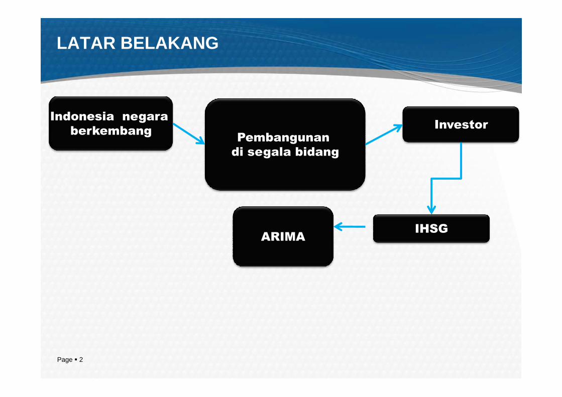
LATAR BELAKANG
Pembangunan
di segala bidang
InvestorIndonesia negara
berkembang
Page � 2
IHSGARIMA
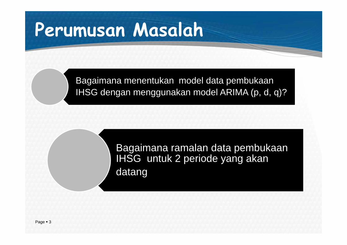
Perumusan Masalah
Bagaimana menentukan model data pembukaan IHSG dengan menggunakan model ARIMA (p, d, q)?
Page � 3
Bagaimana ramalan data pembukaan IHSG untuk 2 periode yang akandatang
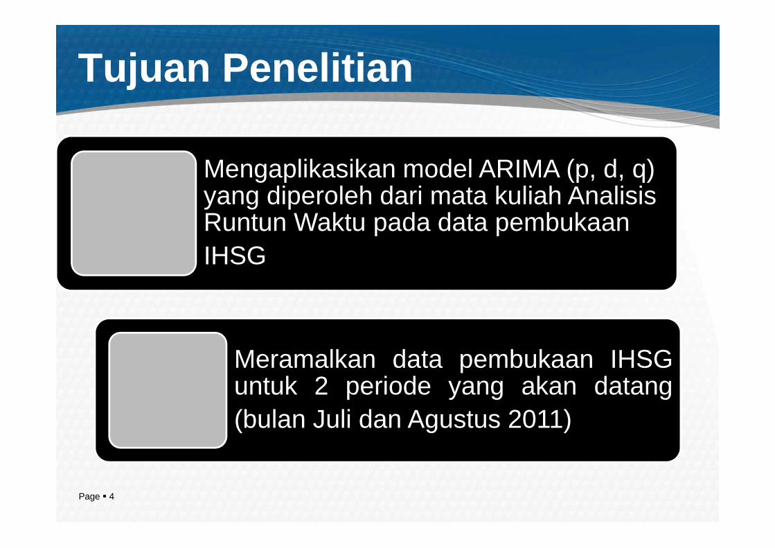
Tujuan Penelitian
Mengaplikasikan model ARIMA (p, d, q) yang diperoleh dari mata kuliah AnalisisRuntun Waktu pada data pembukaan IHSG
Page � 4
Meramalkan data pembukaan IHSGuntuk 2 periode yang akan datang(bulan Juli dan Agustus 2011)
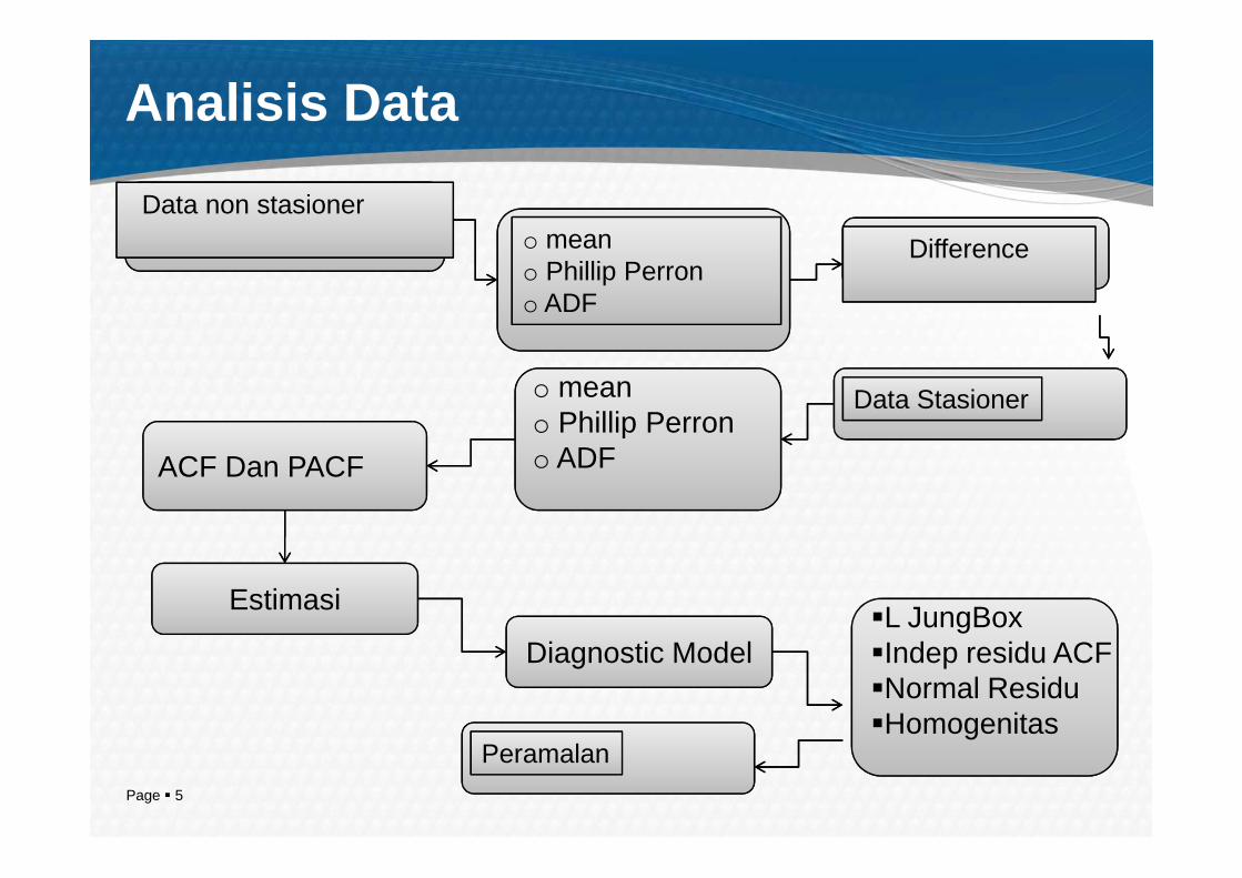
Analisis Data
o meano Phillip Perron
Data non stasionero meano Phillip Perrono ADF
Difference
Data Stasioner
Page � 5
oo ADFACF Dan PACF
Diagnostic Model�L JungBox�Indep residu ACF�Normal Residu�Homogenitas
Estimasi
Peramalan
4000
3500
3000MA PE 17
A ccu racy M easu res
A ctual
F its
Var iab le
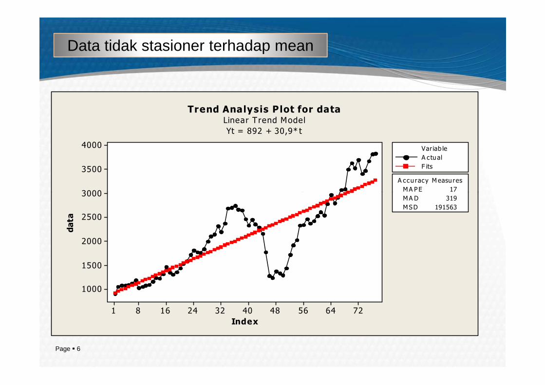
Trend Analysis Plot for dataLinear T rend Model
Yt = 892 + 30,9* t
Data tidak stasioner terhadap mean
Page � 6
726456484032241681
3000
2500
2000
1500
1000
Index
data
MA PE 17
MA D 319
MSD 191563

1,0
0,8
0,6
0,4
0,2
tion
Autocorrelation Function for data(with 5% significance limits for the autocorrelations)
Plot Fungsi Autokorelasi
Page � 7
757065605550454035302520151051
0,2
0,0
-0,2
-0,4
-0,6
-0,8
-1,0
Lag
Autocorrelat
1,0
0,8
0,6
0,4
0,2relation
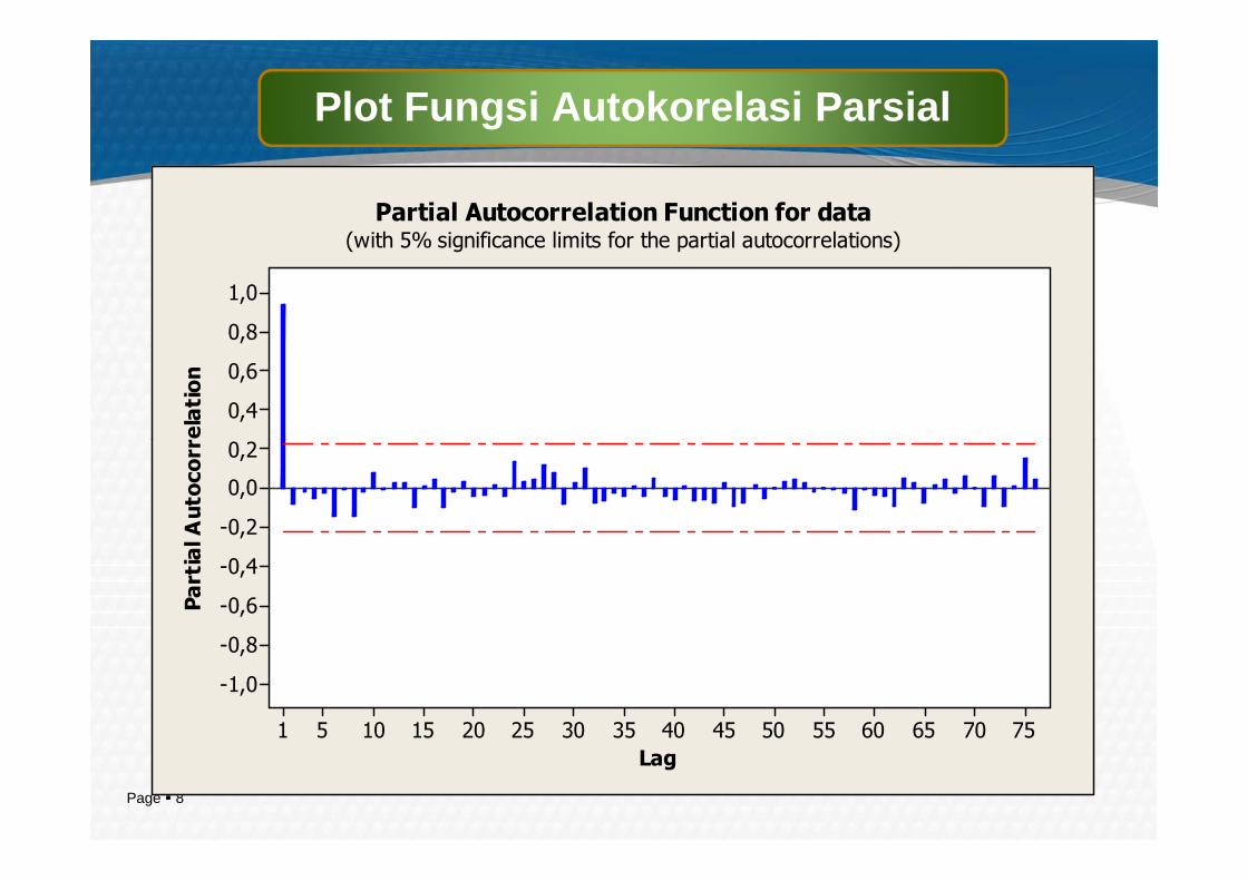
Partial Autocorrelation Function for data(with 5% significance limits for the partial autocorrelations)
Plot Fungsi Autokorelasi Parsial
Page � 8
757065605550454035302520151051
0,2
0,0
-0,2
-0,4
-0,6
-0,8
-1,0
Lag
Partial Autocorr
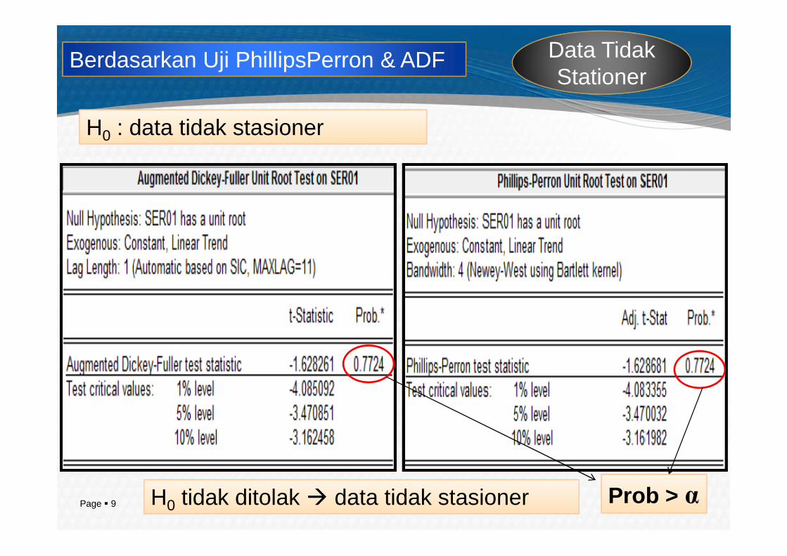
Data TidakStationer
H0 : data tidak stasioner
Berdasarkan Uji PhillipsPerron & ADF
Page � 9 Prob > αH0 tidak ditolak � data tidak stasioner
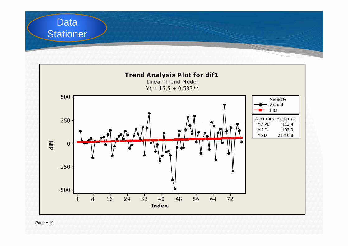
Data Stationer
500
250MA PE 113,4
A ccu racy Measu res
A c tual
F its
Var iab le
Trend Analysis P lot for dif1Linear T rend Model
Yt = 15,5 + 0,583* t
Page � 10
726456484032241681
250
0
-250
-500
Index
dif1
MA PE 113,4
MA D 107,0
MSD 21310,8
1,0
0,8
0,6
0,4
0,2
ion
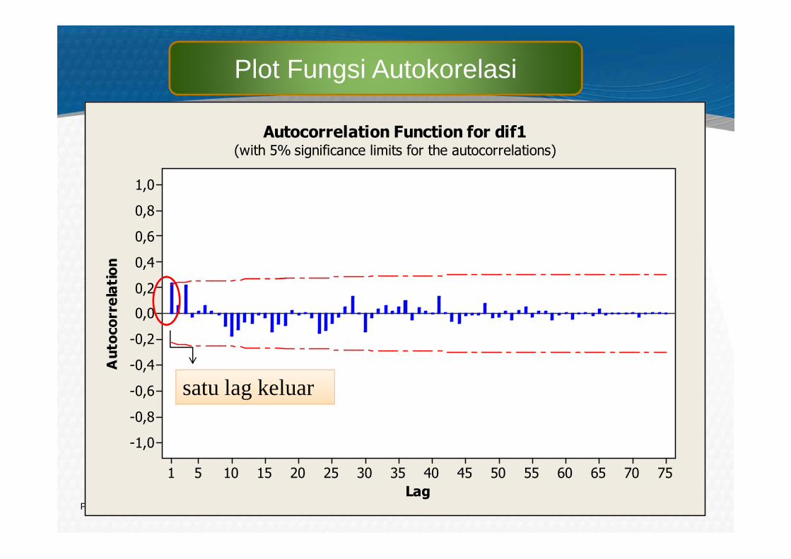
Autocorrelation Function for dif1(with 5% significance limits for the autocorrelations)
Plot Fungsi Autokorelasi
Page � 11
757065605550454035302520151051
0,2
0,0
-0,2
-0,4
-0,6
-0,8
-1,0
Lag
Autocorrelat
satu lag keluar

1,0
0,8
0,6
0,4
elation
Partial Autocorrelation Function for dif1(with 5% significance limits for the partial autocorrelations)
Plot Fungsi Autokorelasi Parsial
Page � 12
757065605550454035302520151051
0,2
0,0
-0,2
-0,4
-0,6
-0,8
-1,0
Lag
Partial Autocorre
satu lag keluar
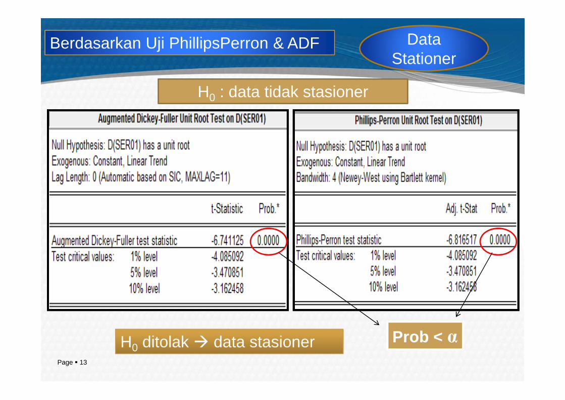
Data Stationer
Berdasarkan Uji PhillipsPerron & ADF
H0 : data tidak stasioner
Page � 13
Prob < αH0 ditolak � data stasioner
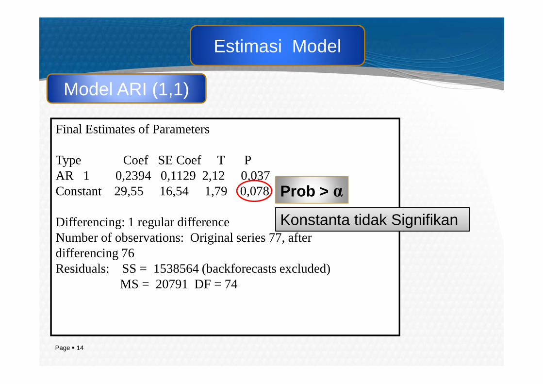
Estimasi Model
Final Estimates of Parameters
Type Coef SE Coef T PAR 1 0,2394 0,1129 2,12 0,037Constant 29,55 16,54 1,79 0,078
Model ARI (1,1)
Prob > α
Page � 14
Constant 29,55 16,54 1,79 0,078
Differencing: 1 regular differenceNumber of observations: Original series 77, after differencing 76Residuals: SS = 1538564 (backforecasts excluded)
MS = 20791 DF = 74
Prob > α
Konstanta tidak Signifikan

Type Coef SE Coef T PMA 1 -0,2766 0,1118 -2,47 0,016Constant 38,75 21,06 1,84 0,070
Estimasi Model
Model IMA (1,1)
Final Estimates of Parameters
Prob > α
Page � 15
Constant 38,75 21,06 1,84 0,070
Differencing: 1 regular differenceNumber of observations: Original series 77, after differencing 76Residuals: SS = 1531747 (backforecasts excluded)
MS = 20699 DF = 74
Prob > α
Konstanta tidak Signifikan
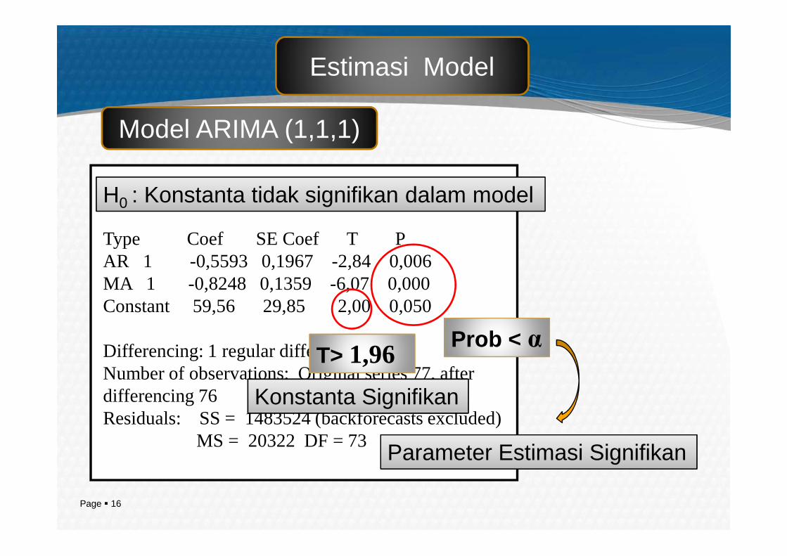
Final Estimates of Parameters
Type Coef SE Coef T PAR 1 -0,5593 0,1967 -2,84 0,006MA 1 -0,8248 0,1359 -6,07 0,000
Model ARIMA (1,1,1)
Estimasi Model
H0 : Konstanta tidak signifikan dalam model
Page � 16
MA 1 -0,8248 0,1359 -6,07 0,000Constant 59,56 29,85 2,00 0,050
Differencing: 1 regular differenceNumber of observations: Original series 77, after differencing 76Residuals: SS = 1483524 (backforecasts excluded)
MS = 20322 DF = 73
Prob < α
Parameter Estimasi Signifikan
T> 1,96
Konstanta Signifikan
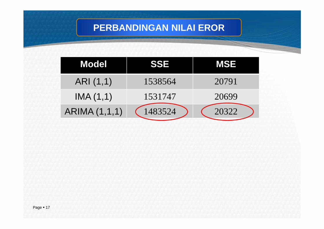
PERBANDINGAN NILAI EROR
Model SSE MSE
ARI (1,1) 1538564 20791
IMA (1,1) 1531747 20699
ARIMA (1,1,1) 1483524 20322
Page � 17
ARIMA (1,1,1) 1483524 20322
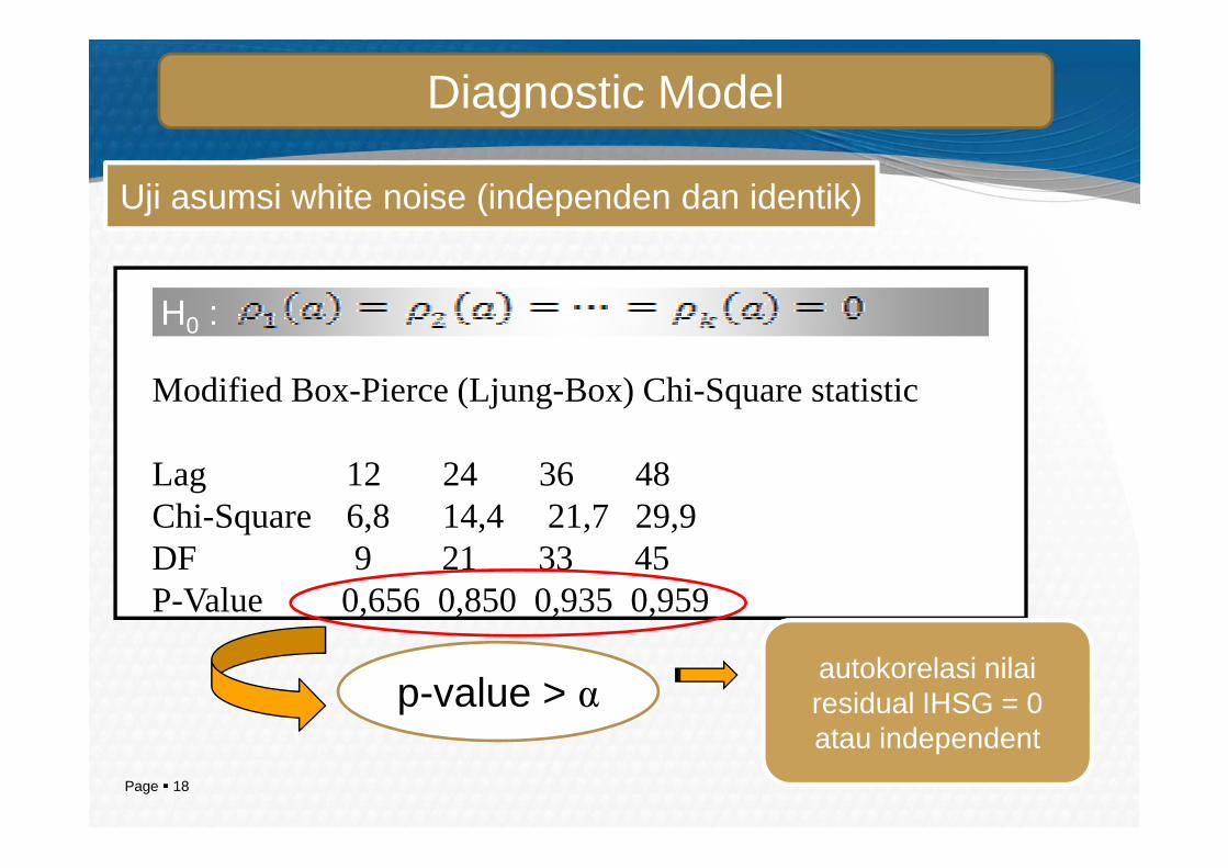
Diagnostic Model
Uji asumsi white noise (independen dan identik)
Modified Box-Pierce (Ljung-Box) Chi-Square statistic
H0 :
Page � 18
Lag 12 24 36 48Chi-Square 6,8 14,4 21,7 29,9DF 9 21 33 45P-Value 0,656 0,850 0,935 0,959
p-value > αautokorelasi nilairesidual IHSG = 0 atau independent
1 ,0
0 ,8
0 ,6
0 ,4
on
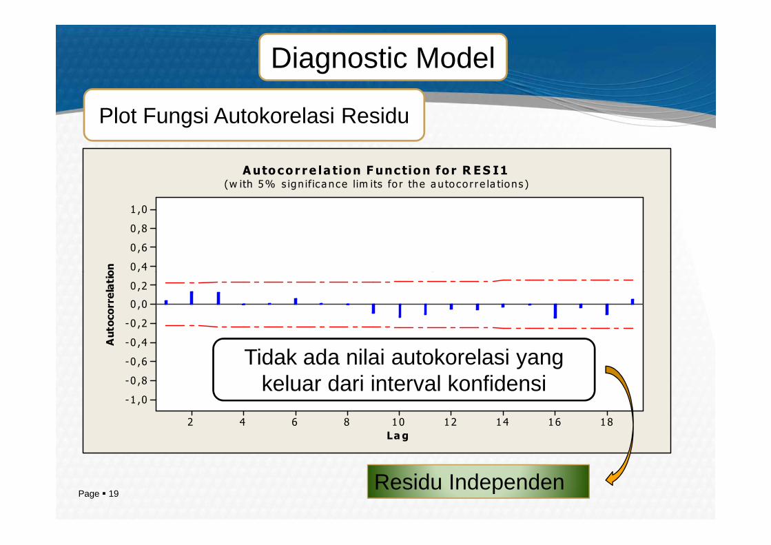
Autoco r r e la tion F unc tion fo r R ES I1(w ith 5% s ign ifica nce lim its fo r the a u to co r r e la tions )
Diagnostic Model
Plot Fungsi Autokorelasi Residu
Page � 19
18161412108642
0 ,2
0 ,0
-0 ,2
-0 ,4
-0 ,6
-0 ,8
-1 ,0
La g
Autocorrelatio
Tidak ada nilai autokorelasi yang keluar dari interval konfidensi
Residu Independen
99,9
99
95
90
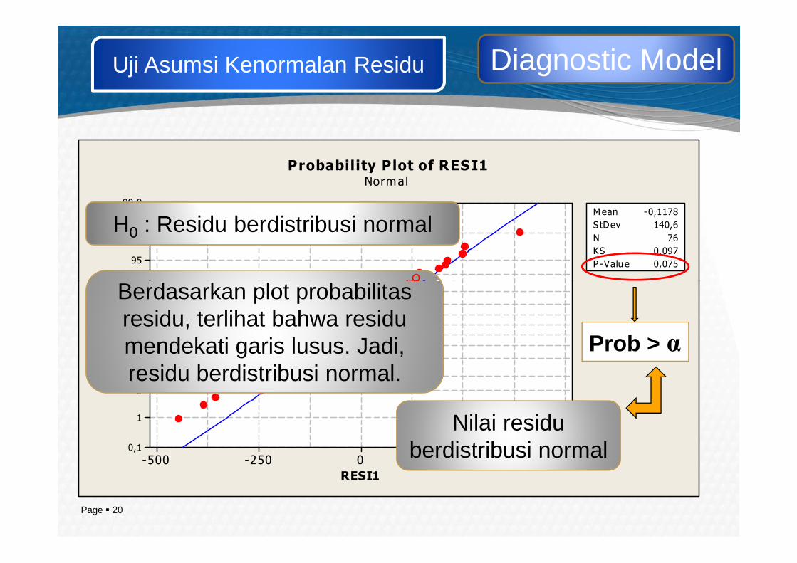
Mean -0,1178
S tDev 140,6
N 76
KS 0,097
P -Value 0,075
Probability Plot of RESI1Normal
Diagnostic ModelUji Asumsi Kenormalan Residu
Berdasarkan plot probabilitas
H0 : Residu berdistribusi normal
Page � 20
5002500-250-500
80
7060504030
20
10
5
1
0,1
RESI1
Percent
Berdasarkan plot probabilitasresidu, terlihat bahwa residumendekati garis lusus. Jadi, residu berdistribusi normal.
Prob > α
Nilai residuberdistribusi normal
400
300
200
100
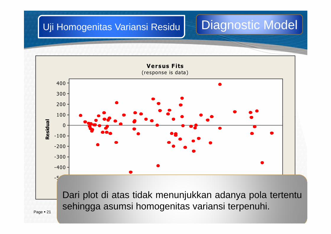
Versus F its(response is da ta)
Diagnostic ModelUji Homogenitas Variansi Residu
Page � 21
4000350030002500200015001000
100
0
-100
-200
-300
-400
-500
Fit ted Va lue
Residual
Dari plot di atas tidak menunjukkan adanya pola tertentusehingga asumsi homogenitas variansi terpenuhi.
PERAMALANPERAMALANPERAMALANPERAMALAN
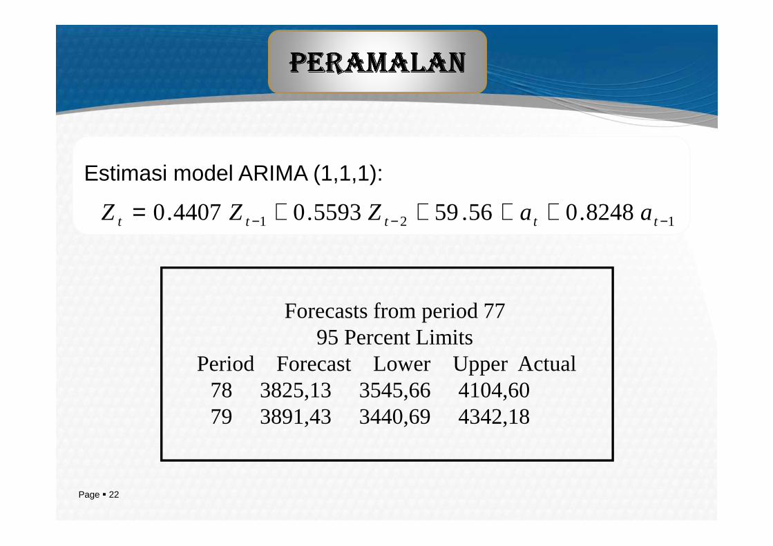
Estimasi model ARIMA (1,1,1):
121 8248.056.595593.04407.0 −−− ++++= ttttt aaZZZ
Page � 22
Forecasts from period 7795 Percent Limits
Period Forecast Lower Upper Actual78 3825,13 3545,66 4104,6079 3891,43 3440,69 4342,18
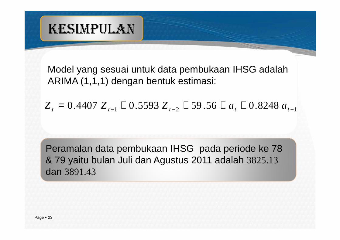
KESIMPULAN
Model yang sesuai untuk data pembukaan IHSG adalahARIMA (1,1,1) dengan bentuk estimasi:
121 8248.056.595593.04407.0 −−− ++++= ttttt aaZZZ
Page � 23
Peramalan data pembukaan IHSG pada periode ke 78 & 79 yaitu bulan Juli dan Agustus 2011 adalah 3825.13 dan 3891.43

Company LOGO
TERIMA KASIH
www.company.com