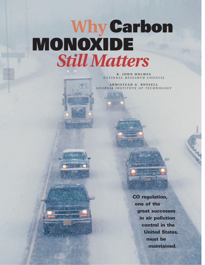
CO regulation, one of the great successes in air pollution control in the United States, must be maintained.

K . J O H N H O L M E S N A T I O N A L R E S E A R C H C O U N C I L

A R M I S T E A D G . R U S S E L LG E O R G I A I N S T I T U T E O F T E C H N O L O G Y

Why Carbon MONOXIDE

Still Matters

Legends and myths of tragic events stemmingfrom carbon monoxide (CO) poisoning canbe traced back thousands of years. CO gen-erally occurs when insufficient oxygen isavailable during combustion of carbon-based fuels. Incidents of CO poisoning in-

creased with the advent of coal and industrialization,thereby linking the toxic gas to the development ofcivilization itself (1, 2). By the early part of the 20thcentury, CO was recognized as a significant occupa-tional health hazard and, by the 1950s, was seen asan indicator of poor air quality in urban areas, re-sulting from motor vehicle emissions.

When CO emissions were first regulated in theUnited States in the 1960s, elevated concentrationswere widespread and long-lasting. Cities such as Den-ver, Colo.; Lynwood, Calif.; and Fairbanks, Alaska,have experienced hundreds of days with high CO peryear. In 1965, Chicago had an average CO concen-tration of 17 ppm, almost twice the current 8-h stan-dard. Following requirements for “criteria pollutants”established under the 1970 Amendments to the CleanAir Act (CAA), the U.S. EPA in 1971 designated health-based National Ambient Air Quality Standards(NAAQS) for ambient CO concentrations at 9 ppm foran 8-h average and 35 ppm for a 1-h average. Accord-ing to a 1977 National Research Council (NRC) study,CO was “probably the most publicized and bestknown criteria pollutant,” in part because of its acuteeffects (2). Substantial controls on automobile COemissions were introduced, and reducing CO pollu-tion became central to air quality management ef-forts in many locations.

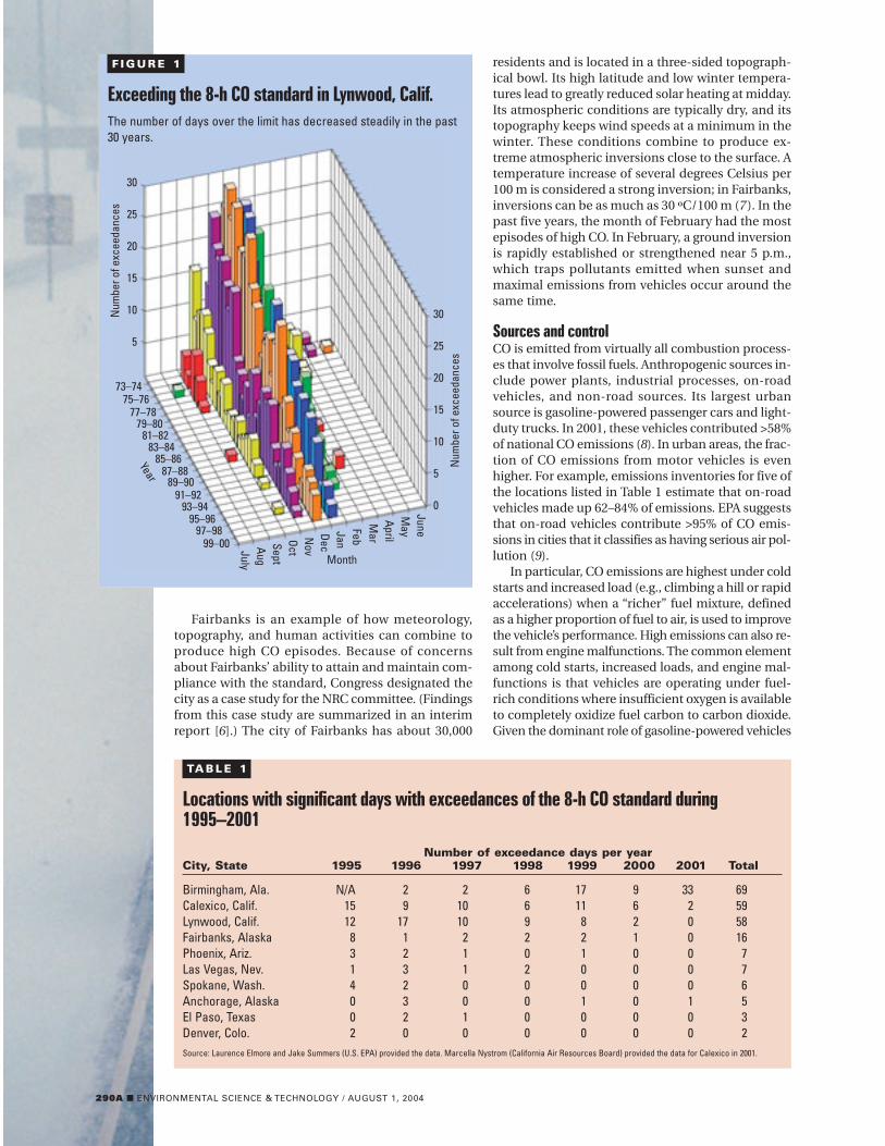
Because ambient standards for CO have beenlargely attained and the estimates of its health im-pacts are much smaller than those from the otherpollutants, contemporary air quality management inthe United States now focuses on attaining newNAAQS for tropospheric ozone and fine particulatematter (PM2.5) and on managing air toxics (3, 4).Figure 1, for example, displays the dramatic reductionin the number of days that exceeded standards inLynwood since the early 1970s.

However, as of 2001, some locations with prob-lematic meteorological and topographical conditionscontinue to occasionally violate the 8-h NAAQS for CO.In its fiscal 2001 appropriations for EPA, Congress askedNRC to study the issue. The NRC Committee on CarbonMonoxide Episodes in Meteorological and Topographi-cal Problem Areas met in many affected locations tohear from experts on local conditions and national andlocal controls. The committee’s findings and recom-mendations are described in Managing Carbon Monox-ide in Meteorological and Topographical Problem Areas(5), which we summarize in this article.

Meteorological and topographical conditionsThe committee recognized that all areas with air qual-ity problems—whether from CO or other pollutants—have a component of physical geography that makesexceedances more likely. This study focused on areassubject to severe winter inversions and low windspeeds that, in combination with confined topogra-phy and significant localized emissions, are extremelyeffective in trapping the products of incomplete com-bustion, including CO. These conditions can occurnot only within major metropolitan areas, such asLynwood, but also in smaller cities, such as Fairbanksand Kalispell, Mont. Except for Birmingham, Ala., allthe locations shown in Table 1 are west of the Missis-sippi and experience the most severe inversion con-ditions in the winter. The CO problem in Birminghamis different. It is not seasonally dependent, but rathercaused by a single point source that produces violationswhen wind conditions direct emissions toward a near-by monitor. Table 1 focuses on areas with wintertimeproblems. It does not include exceedances in Weirton,W.Va., where, like Birmingham, CO problems arelinked with operational malfunctions at a single facility.

Meteorological and topographical conditions in-fluence CO concentrations through effects on verticalmixing, wind speeds, temperature, humidity, and emis-sions. Atmospheric inversions occur when the tem-perature of the atmosphere increases with altitude andgreatly reduces vertical mixing in the atmosphere.Combined with low wind speeds, inversions preventair circulation because colder air is trapped near theground by the warmer air above. Low humidity playsa role by allowing more infrared radiation from theearth’s surface to pass into space, rapidly reducingground-level temperature and producing inversionsclose to the surface after sundown. These meteoro-logical and topographical conditions contribute to thebuildup of a host of pollutants, such as CO, PM2.5, hy-drocarbons (HC), and other atmospheric pollutants.

© 2004 American Chemical Society AUGUST 1, 2004 / ENVIRONMENTAL SCIENCE & TECHNOLOGY ■ 289A

290A ■ ENVIRONMENTAL SCIENCE & TECHNOLOGY / AUGUST 1, 2004

Fairbanks is an example of how meteorology,topography, and human activities can combine toproduce high CO episodes. Because of concernsabout Fairbanks’ ability to attain and maintain com-pliance with the standard, Congress designated thecity as a case study for the NRC committee. (Findingsfrom this case study are summarized in an interimreport [6].) The city of Fairbanks has about 30,000

residents and is located in a three-sided topograph-ical bowl. Its high latitude and low winter tempera-tures lead to greatly reduced solar heating at midday.Its atmospheric conditions are typically dry, and itstopography keeps wind speeds at a minimum in thewinter. These conditions combine to produce ex-treme atmospheric inversions close to the surface. Atemperature increase of several degrees Celsius per100 m is considered a strong inversion; in Fairbanks,inversions can be as much as 30 ºC/100 m (7 ). In thepast five years, the month of February had the mostepisodes of high CO. In February, a ground inversionis rapidly established or strengthened near 5 p.m.,which traps pollutants emitted when sunset andmaximal emissions from vehicles occur around thesame time.

Sources and control CO is emitted from virtually all combustion process-es that involve fossil fuels. Anthropogenic sources in-clude power plants, industrial processes, on-roadvehicles, and non-road sources. Its largest urbansource is gasoline-powered passenger cars and light-duty trucks. In 2001, these vehicles contributed >58%of national CO emissions (8). In urban areas, the frac-tion of CO emissions from motor vehicles is evenhigher. For example, emissions inventories for five ofthe locations listed in Table 1 estimate that on-roadvehicles made up 62–84% of emissions. EPA suggeststhat on-road vehicles contribute >95% of CO emis-sions in cities that it classifies as having serious air pol-lution (9).

In particular, CO emissions are highest under coldstarts and increased load (e.g., climbing a hill or rapidaccelerations) when a “richer” fuel mixture, definedas a higher proportion of fuel to air, is used to improvethe vehicle’s performance. High emissions can also re-sult from engine malfunctions. The common elementamong cold starts, increased loads, and engine mal-functions is that vehicles are operating under fuel-rich conditions where insufficient oxygen is availableto completely oxidize fuel carbon to carbon dioxide.Given the dominant role of gasoline-powered vehicles

TA B L E 1

Locations with significant days with exceedances of the 8-h CO standard during1995–2001

Number of exceedance days per yearCity, State 1995 1996 1997 1998 1999 2000 2001 Total

Birmingham, Ala. N/A 2 2 6 17 9 33 69Calexico, Calif. 15 9 10 6 11 6 2 59Lynwood, Calif. 12 17 10 9 8 2 0 58Fairbanks, Alaska 8 1 2 2 2 1 0 16Phoenix, Ariz. 3 2 1 0 1 0 0 7Las Vegas, Nev. 1 3 1 2 0 0 0 7Spokane, Wash. 4 2 0 0 0 0 0 6Anchorage, Alaska 0 3 0 0 1 0 1 5El Paso, Texas 0 2 1 0 0 0 0 3Denver, Colo. 2 0 0 0 0 0 0 2Source: Laurence Elmore and Jake Summers (U.S. EPA) provided the data. Marcella Nystrom (California Air Resources Board) provided the data for Calexico in 2001.

30

25

20

15

10

5

Num

ber o

f exc

eeda

nces

Num

ber o

f exc

eeda

nces

Month

Year

30

25

20

15

10

5

0

JulyAug

SeptOctN

ovDecJanFeb

Mar

AprilM

ayJune

73–7475–76

77–7879–80

81–8283–84

85–8687–88

89–9091–92

93–9495–96

97–9899–00

F I G U R E 1

Exceeding the 8-h CO standard in Lynwood, Calif.The number of days over the limit has decreased steadily in the past30 years.

in emissions, CO management has focused largely onimproving combustion efficiencies and post-com-bustion catalyst controls for these vehicles.

New motor vehicle emissions standards and con-trols. Lowering new-vehicle emissions certificationstandards has resulted in the most significant COemissions reductions. Passenger cars since model year1981 must not emit more than 3.4 g CO/mile for cer-tification tests run at standard temperatures (68–86 °F). Before controls were introduced, average new-vehicle emissions were 84 g/mile! A separate new-vehicle emissions standard limits passenger cars builtsince 1994 to 10 g CO/mile at 20 °F. Both the normaland cold temperature standards were met through acombination of combustion and post-combustioncontrols. Combustion controls for CO primarily in-volve reducing the time the engine operates in fuel-rich conditions through sophisticated on-boardcomputers, oxygen sensors, and fuel-injection sys-tems. Post-combustion controls include catalytic con-verters that oxidize CO to carbon dioxide before theexhaust exits the tailpipe. Reducing cold-temperatureCO emissions required further refinements in catalystdesign. Both combustion and post-combustion con-trols have a significant impact on other motor vehi-cle emissions, including HC.

In-use emissions controls. During public sessions,the committee heard from state and local officialsabout the programs implemented locally to furthercontrol in-use motor vehicle emissions. Motor vehi-cle emissions inspection and maintenance (I/M) pro-grams and oxygenated fuel programs are the mostcommon methods used locally to augment federalemissions standards. The CAA mandates both I/Mand fuel programs for the worst CO areas. Althoughemissions decreases that arise from I/M and oxy-genated fuel programs probably have fallen short ofthe benefits that were originally projected (10–15),they are pursued as some of the largest potentialsources of emissions reductions beyond new-vehicleemissions standards.

The committee also heard about other location-specific motor vehicle controls, which include imple-menting programs to improve traffic flow, encouragingengine preheater use, and using alert day or volun-tary trip reduction strategies. For example, catalyticconverters on vehicles in Fairbanks can take 10 minor more to warm up and become fully effective dur-ing winter (16). Cold-start emissions in Fairbanks areestimated to contribute 45% of all motor vehicle emis-sions (17). The local government, the Fairbanks NorthStar Borough, is making substantial efforts to controlthese emissions by making available and encourag-

ing the use of electric outlets for engine-preheat de-vices known as “plug-ins”. These devices improve ve-hicle starting and greatly reduce the time needed forthe catalyst to become fully operational.

Control of other sources. There is much less focuson controls of CO emissions from other industrialand nonroad sources. However, these other sourcesincreasingly contribute a larger fraction of emissions.Since CO problems can be caused by fairly localizedemissions sources, there also are instances when asingle large stationary source is the cause of the prob-lem and the sole focus of controls. For example, inBirmingham and Weirton, the CO-control strategy fo-cuses on modifying the operations of a single indus-trial production facility (18).

Changes in emissions and air quality. Accordingto EPA, nationwide CO emissions were reduced by32% between 1982 and 2001 (8). Light-duty gasoline-vehicle emissions decreased by 43%, and all othersources combined decreased by 8% during the sametime period (8). The improvement in CO emissionsoccurred despite an approximately 43% increase invehicle miles traveled (VMT) in the United States overthe same period (19).

Trends in national average ambient CO concen-trations do not mirror trends in nationwide emis-sions. Using the average of the second-highest 8-hannual concentration from >200 monitoring sites,EPA estimates that the average ambient CO concen-tration has declined by 65% during the 1983–2002 pe-riod (9). This amount is substantially more than theestimated reduction in national CO emissions. Asshown by various studies of vehicle emissions and airquality, some of the discrepancy may be due to un-certainties and inaccuracies in models and data usedto estimate national and local emissions inventories(5, 20–24). Because most CO monitors are located inurban areas, a larger issue may be that changes in airquality tend to track changes in urban air emissionsrather than in total emissions. Because light-duty ve-hicles dominate urban emissions, the improvementsin ambient CO concentrations disproportionately re-flect reductions in emissions from this source.

History of criteria pollutants under NAAQS As defined in the Clean Air Act Amendments of 1970, cri-teria pollutants are air pollutants emitted from numerousor diverse stationary or mobile sources. The amend-ments direct the U.S. EPA to set National Ambient AirQuality Standards (NAAQS) to protect human healthand public welfare. The original criteria pollutantswere carbon monoxide, total suspended particulatematter, sulfur dioxide, photochemical oxidants, hydro-carbons, and nitrogen oxides. Lead was added to thelist in 1976, ozone replaced photochemical oxidants in1979, and hydrocarbons were dropped in 1983. Totalsuspended particulate matter was revised in 1987 toinclude only particles with an equivalent aerodynamicparticle diameter of ≤10 micrometers (PM10). A sepa-rate standard for particles with an equivalent aerody-namic particle diameter of ≤2.5 micrometers (PM2.5)was adopted in 1997.

AUGUST 1, 2004 / ENVIRONMENTAL SCIENCE & TECHNOLOGY ■ 291A

Lowering new-vehicle

emissions certification

standards has resulted in

the most significant CO

emissions reductions.

292A ■ ENVIRONMENTAL SCIENCE & TECHNOLOGY / AUGUST 1, 2004

Air quality managementIn the near term, the committee found that conditionsfor CO attainment in those few areas that continueto experience violations and those that have recent-ly come into attainment should continue to improve.The biggest factor is the continuing decline in motorvehicle CO emissions rates. Yet, this decline occurswithout the tightening of passenger car emissionsstandards for CO at normal temperatures (68–86 °F)since 1981 and with VMT continuing to increase.Improvements are due to fleet turnover, with anincreasing fraction of vehicles in the fleet being cer-tified to tighter CO standards, including cold temp-erature (20 °F) standards. Improvements are also acollateral benefit of tightening emissions standards forHC and nitrogen oxide (NOx) emissions. Some of thetechnologies adopted to meet these standards—especially for HC control—reduce CO emissions.Future regulations affecting CO emissions rates from

motor vehicles include the new Tier 2 standards thattighten NOx and HC emissions standards and reducefuel sulfur content (25, 26).

How long will advances in motor vehicle emis-sions control technology reduce CO emissions ratesfaster than VMT increases? Some information pre-sented to the committee suggested that regional COemissions will continue to decrease well into the fu-ture (27, 28), whereas other sources showed that emis-sions would start to increase again as early as 2005(29, 30). The continued decline in CO emissions willdepend not only on the rate of increase in VMT butalso on the extent to which technologies adopted toreduce NOx and HC emissions rates will reduce COemissions rates. However, for locations outside ofthose listed in Table 1, the increase in CO emissions,if it occurs at all, may occur when ambient concen-trations are well below the NAAQS.

At least some locations listed in Table 1 will re-main vulnerable to exceedances of the 8-h NAAQSfor CO because of meteorological and topographicalconditions that produce severe winter inversions.Future large increases in population might compoundthese adverse natural conditions, especially in smallcities such as Fairbanks, whose populations can surgewith the initiation of a single large project such as theconstruction of military facilities or a trans-nationalnatural gas pipeline. The role of meteorological andtopographical conditions in causing CO exceedancesprompted some local officials to suggest that these lo-cations should be granted some form of exemptionfrom the CAA. However, the committee concludedthat a similar argument could be made for other re-gions with regard to various air quality problems.Thus, the committee recommended that local airquality management agencies continue to enhanceprograms to identify and repair or remove high-emit-ting vehicles and to improve programs tailored tolocal conditions, such as the Fairbanks plug-in pro-gram. Although new-vehicle emissions standards forHC and NOx emissions control should provide a col-lateral benefit for CO, testing should confirm the ex-tent to which emissions reductions for CO actuallyoccur, especially at temperatures <20 °F. A completelisting of the committee’s recommendations is avail-able in its report (5).

Health Benefits. The committee found that EPApresented strong scientific evidence in support of thehealth-based NAAQS (31). In addition, recent epi-demiological studies have correlated high CO con-centrations with other adverse human health effects,such as heart disease, childhood developmental ab-normalities, and fetal loss. Some of these effects havebeen correlated with ambient CO concentrationsbelow the NAAQS (32, 33). However, CO is not pro-duced alone, and epidemiological studies have diffi-culty separating the effects of CO from those of otherpollutants that are often associated with CO (such asbenzene, 1,3-butadiene, aldehydes, and various com-ponents of PM2.5). CO is also a precursor to ozoneformation in urban areas (5).

A substantial collateral health benefit from reducingCO new-vehicle emissions standards is the decline inaccidental deaths due to acute CO poisoning. CO is

1.0

0.9

0.8

0.7

0.6

0.5

0.4

0.3

0.2

0.1

0

Hour of the day

CO (p

pm),

Benz

ene/

3 (p

pb)

1 2 3 4 5 6 7 8 9 10 11 12 13 14 15 16 17 18 19 20 21 22 23 24

(a)

1.0

0.8

0.6

0.4

0.2

0.0

Distance to the 405 Freeway (m)

Rela

tive

conc

entra

tion

(b)

–300Upwind –200 –100 0 100 200 300 Downwind

Relative massCarbon monoxideParticle numberBlack carbon

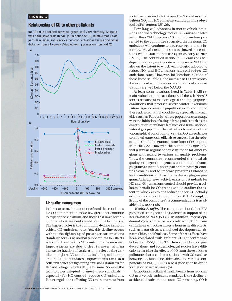
F I G U R E 2

Relationship of CO to other pollutants (a) CO (blue line) and benzene (green line) vary diurnally. Adaptedwith permission from Ref 41. (b) Variation of CO, relative mass, totalparticle number, and black carbon concentrations versus downwinddistance from a freeway. Adapted with permission from Ref 42.

AUGUST 1, 2004 / ENVIRONMENTAL SCIENCE & TECHNOLOGY ■ 293A

unique among criteria pollutants because of its signif-icance for both ambient air quality management andpublic safety. In particular, exposures to mobile-sourceemissions encompass these two areas of public-healthmanagement. A recent study estimated that >11,000deaths from accidental CO poisoning have been avoid-ed over the 1968–1998 period because of the more strin-gent vehicle emissions standards (34). This “collateral”benefit is not accounted for in EPA’s recent reports onthe benefits and costs of the CAA (3, 4), yet it dwarfs theestimated direct benefits ascribed to CO control.

CO as an indicator. The buildup of CO in the am-bient environment demonstrates the role that mete-orology and topography have on ground-levelemissions (especially those from motor vehicles) dur-ing winter under conditions of low vertical mixing. Assuch, CO can indicate other directly emitted mobile-source pollutants, such as toxic HCs and componentsof PM. Figure 2 shows that the relationship to otherpollutants can be strong. This figure shows the cor-relation between benzene and CO concentrations bytime of day and indicates how CO and two aspects of

PM (particle number and black carbon) disperse froma highway.

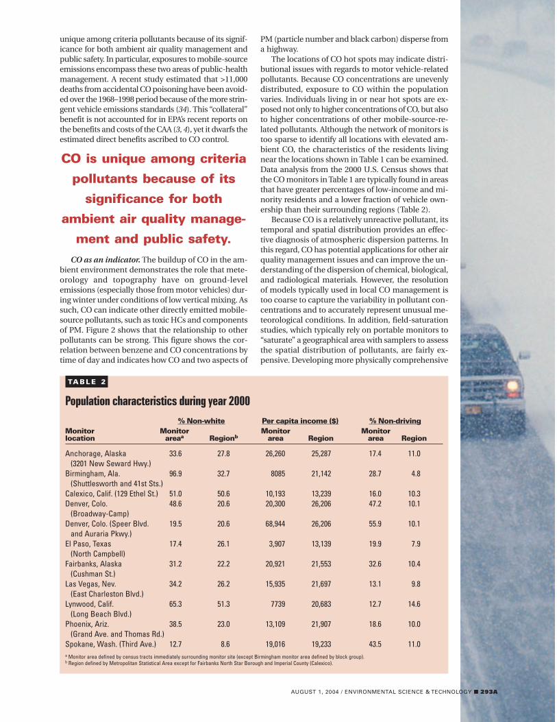
The locations of CO hot spots may indicate distri-butional issues with regards to motor vehicle-relatedpollutants. Because CO concentrations are unevenlydistributed, exposure to CO within the populationvaries. Individuals living in or near hot spots are ex-posed not only to higher concentrations of CO, but alsoto higher concentrations of other mobile-source-re-lated pollutants. Although the network of monitors istoo sparse to identify all locations with elevated am-bient CO, the characteristics of the residents livingnear the locations shown in Table 1 can be examined.Data analysis from the 2000 U.S. Census shows thatthe CO monitors in Table 1 are typically found in areasthat have greater percentages of low-income and mi-nority residents and a lower fraction of vehicle own-ership than their surrounding regions (Table 2).

Because CO is a relatively unreactive pollutant, itstemporal and spatial distribution provides an effec-tive diagnosis of atmospheric dispersion patterns. Inthis regard, CO has potential applications for other airquality management issues and can improve the un-derstanding of the dispersion of chemical, biological,and radiological materials. However, the resolutionof models typically used in local CO management istoo coarse to capture the variability in pollutant con-centrations and to accurately represent unusual me-teorological conditions. In addition, field-saturationstudies, which typically rely on portable monitors to“saturate” a geographical area with samplers to assessthe spatial distribution of pollutants, are fairly ex-pensive. Developing more physically comprehensive

TA B L E 2

Population characteristics during year 2000% Non-white Per capita income ($) % Non-driving

Monitor Monitor Monitor Monitor location areaa Regionb area Region area Region

Anchorage, Alaska 33.6 27.8 26,260 25,287 17.4 11.0(3201 New Seward Hwy.)

Birmingham, Ala. 96.9 32.7 8085 21,142 28.7 4.8(Shuttlesworth and 41st Sts.)

Calexico, Calif. (129 Ethel St.) 51.0 50.6 10,193 13,239 16.0 10.3Denver, Colo. 48.6 20.6 20,300 26,206 47.2 10.1

(Broadway-Camp)Denver, Colo. (Speer Blvd. 19.5 20.6 68,944 26,206 55.9 10.1

and Auraria Pkwy.)El Paso, Texas 17.4 26.1 3,907 13,139 19.9 7.9

(North Campbell)Fairbanks, Alaska 31.2 22.2 20,921 21,553 32.6 10.4

(Cushman St.)Las Vegas, Nev. 34.2 26.2 15,935 21,697 13.1 9.8

(East Charleston Blvd.)Lynwood, Calif. 65.3 51.3 7739 20,683 12.7 14.6

(Long Beach Blvd.)Phoenix, Ariz. 38.5 23.0 13,109 21,907 18.6 10.0

(Grand Ave. and Thomas Rd.)Spokane, Wash. (Third Ave.) 12.7 8.6 19,016 19,233 43.5 11.0a Monitor area defined by census tracts immediately surrounding monitor site (except Birmingham monitor area defined by block group).b Region defined by Metropolitan Statistical Area except for Fairbanks North Star Borough and Imperial County (Calexico).

CO is unique among criteria

pollutants because of its

significance for both

ambient air quality manage-

ment and public safety.

294A ■ ENVIRONMENTAL SCIENCE & TECHNOLOGY / AUGUST 1, 2004

models that can accurately simulate the variability ofCO and evaluating such models against field datawould be useful for assessing atmospheric dispersionand human exposure to various airborne materials.

Some believe that CO would be most useful in mi-croscale setting where polluted concentrations varydramatically over short distances, for example, withdistance from a roadway. This setting is importantbecause some studies have found a link betweenhealth impacts and proximity to major roadways (35–37), although other studies have found no such cor-relation (38–40). CO is less reliable in representing re-gional distributions of other pollutants and, atregional scales, is probably a poor indicator of mo-bile-source air toxics, such as formaldehyde and ac-etaldehyde, that react rapidly and have substantialsources in the atmosphere.

Where do we go from here? Extremely high ambient CO pollution has disappearedfrom most urban areas in the United States, greatlyreducing human exposure to ambient CO. However,in a few major metropolitan areas and smaller cities,it remains a significant part of air quality manage-ment activities. The common element for most ofthese locations is a susceptibility to wintertime in-versions that limit dilution of motor vehicle emissions.

Given the reduced number of air quality violationsand newly promulgated standards and regulationsfor PM, ozone, and air toxics, CO will not be the focusof air quality management. Consequently, new con-trols will be directed at other pollutants. Nevertheless,in addition to health concerns, continued studies ofCO remain critical for understanding the impact ofmeteorological and topographical conditions on airpollution, particularly during the winter; the spatialand temporal distribution of pollution; the relation-ship between atmospheric concentrations andhuman exposures to motor vehicle-related pollution;and how increases in VMT and changes in the char-acteristics of the vehicle fleet alter motor vehicle emis-sion trends.

K. John Holmes is a senior staff officer with the NationalResearch Council’s Board on Environmental Studies andToxicology, where he is involved in studies on automo-bile emissions and other air quality issues. Armistead G.Russell is a professor at the Georgia Institute of Tech-nology and chaired the NRC Committee on Carbon Mon-oxide Episodes in Meteorological and TopographicalProblem Areas.

References (1) Lewin, L. Carbon Monoxide Poisoning: A Manual for

Physicians, Engineers, and Accident Investigators; Springer-Verlag: Berlin, Germany, 1920.

(2) Carbon Monoxide. Medical and Biologic Effects of Environ-mental Pollutants; National Research Council, NationalAcademy of Sciences: Washington, DC, 1977.

(3) Final Report to Congress on Benefits and Costs of the CleanAir Act, 1970 to 1990; U.S. EPA: Washington, DC, 1997.

(4) Final Report to Congress on Benefits and Costs of the CleanAir Act, 1990 to 2010; U.S. EPA: Washington, DC, 1999.

(5) Managing Carbon Monoxide Pollution in Meteorologicaland Topographical Problem Areas; National ResearchCouncil, National Academy Press: Washington, DC, 2003.

(6) The Ongoing Challenge of Managing Carbon Monoxide

Pollution in Fairbanks, Alaska; National Research Council,National Academy Press: Washington, DC, 2003.

(7) Bowling, S. A. J. Clim. Appl. Met. 1986, 25, 22–34.(8) Average Annual Emissions, All Criteria Pollutants Years In-

cluding 1970–2001; U.S. EPA: Washington, DC, 2003. (9) Latest Findings on National Air Quality 2002 Status and

Trends; Office of Air Quality Planning and Standards, U.S.EPA: Washington, DC, 2003.

(10) Toxicological and Performance Aspects of OxygenatedMotor Vehicle Fuels; National Research Council, NationalAcademy Press: Washington, DC, 1996.

(11) Evaluating Vehicle Emissions Inspection and MaintenancePrograms; National Research Council, National AcademyPress: Washington, DC, 2001.

(12) Holmes, K. J.; Cicerone, R. J. EM 2002, July, 21–28.(13) Wenzel, T. Environ. Sci. Policy 2001, 6, 359–376.(14) Stedman, D. H.; et al. Environ. Sci. Technol. 1997, 31, 927–

931.(15) Interagency Assessment of Oxygenated Fuels; National Sci-

ence and Technology Council, Office of Science and Tech-nology Policy: Washington, DC, 1997.

(16) Analysis of Alaska Vehicle CO Emissions Study Data; SierraResearch, Inc.: Sacramento, CA, 2000.

(17) State Air Quality Control Plan,Vol. 2. Analysis of Problems,Control Actions, Section III.C: Fairbanks TransportationControl Program; Alaska Department of EnvironmentalConservation: Juneau, AK, 2001.

(18) Air Quality Data Update—2001–2002 Carbon Monoxide;U.S. EPA, Office of Air Quality Planning and Standards:Washington, DC, 2003.

(19) Davis, S. C. Transportation Energy Data Book: Edition 22;Oak Ridge National Laboratory: Oak Ridge, TN, 2002.

(20) Modeling Mobile-Source Emissions; National ResearchCouncil, National Academy Press: Washington, DC, 2000.

(21) Holmes, K. J., Russell, A. G. EM 2001, Feb, 20–28.(22) Watson, J. G.; Chow, J. C.; Fujita, E. M. Atmos. Environ.

2001, 35 (9), 1567–1584.(23) Pollack, A. K.; et al. J. Air Waste Manage. Assoc. 1998, 48,

291–305.(24) Parrish, D. D.; et al. J. Geophys. Res. 2002, 107, D12.(25) Regulatory Impact Analysis: Control of Air Pollution from

New Motor Vehicles: Tier 2 Motor Vehicle Emission Stan-dards and Gasoline Sulfur Control Requirements; U.S. EPA:Washington, DC, 1999.

(26) Air pollution control; new motor and engines: Tier 2 motorvehicle emission standards and gasoline sulfur controlrequirements. Fed. Regist. 2000, 65 (28), 6697–6870.

(27) Albu, S. Presentation at the Fifth Meeting on Carbon Mon-oxide Episodes in Meteorological and Topographical Prob-lem Areas, April 8, 2002, Irvine, CA.

(28) Dana, G. Presentation at the Sixth Meeting on CarbonMonoxide Episodes in Meteorological and TopographicalProblem Areas, July 16, 2002, Missoula, MT.

(29) Carbon Monoxide Redesignation Request and MaintenancePlan for the Denver Metropolitan Area; Colorado Depart-ment of Public Health and Environment: Denver, CO,2000.

(30) Carbon Monoxide Redesignation Request and MaintenancePlan for the New York Metropolitan Area; New York StateDepartment of Environmental Conservation: Albany, NY,1999.

(31) Air Quality Criteria for Carbon Monoxide; U.S. EPA: Wash-ington, DC, 2000.

(32) Ritz, B.; et al. Epidemiology 2000, 11 (5), 502–511.(33) Ritz, B.; et al. Am. J. Epidemiol. 2002, 155 (1), 17–25.(34) Mott, J. A.; et al. J. Am. Med. Assoc. 2002, 288, 988–995.(35) Brunekreef, B. Epidemiology 1997, 8 (3), 298–303.(36) Buckeridge, D. L.; et al. Environ. Health Perspect. 2002,

110 (3), 293–300.(37) Wulhelm, M.; Ritz, R. Environ. Health Perspect. 2003, 111

(2), 207–216.(38) Waldron, G.; Pottle, B.; Dod, J. J. Public Health Med. 1995,

17 (1), 85–89.(39) Magnus, P.; et al. Int. J. Epidemiol. 1998, 27 (6), 995–999.(40) Wilkinson, P.; et al. Thorax 1999, 54 (12), 1070–1074. (41) Williams, M. L. Revue Francaise d’Allergologie et d’Immun-

ologie Clinique 2000, 40, 216–21.(42) Zhu, Y.; et al. J. Air Waste Manage. Assoc. 2002, 52,

1032–1042.