Embed Size (px)
Citation preview
University of California
Los Angeles
Finite generators for countable group actions; Finite
index pairs of equivalence relations; Complexity
measures for recursive programs
A dissertation submitted in partial satisfaction
of the requirements for the degree
Doctor of Philosophy in Mathematics
by
Anush Tserunyan
2013
© Copyright by
Anush Tserunyan
2013
Abstract of the Dissertation
Finite generators for countable group actions; Finite
index pairs of equivalence relations; Complexity
measures for recursive programs
by
Anush Tserunyan
Doctor of Philosophy in Mathematics
University of California, Los Angeles, 2013
Professor Alexander S. Kechris, Co-chair
Professor Itay Neeman, Co-chair
Part 1: Consider a continuous action of a countable group G on a Polish space X. A
countable Borel partition P of X is called a generator if GP ∶= {gP ∶ g ∈ G,P ∈ P} generates
the Borel σ-algebra of X. It was asked by Benjamin Weiss in ’87 whether the nonexistence
of an invariant probability measure implies the existence of a finite generator. The main
result of this part is obtaining a positive answer to this question in case X is σ-compact (in
particular, when X is locally compact). We also show that finite generators always exist
modulo a meager set, answering positively a question raised by Alexander Kechris in the
mid-’90s.
Part 2: We investigate pairs of countable Borel equivalence relations E ⊆ F , where E is
of finite index in F . Our main focus is the well-known problem of whether the treeability
of E implies that of F : we provide various reformulations of it and reduce it to one nat-
ural universal example. In the measure-theoretic context, assuming that F is ergodic, we
characterize the case when E is normal. Finally, in the ergodic case, we characterize the
equivalence relations that arise from almost free actions of virtually free groups.
Part 3: We consider natural complexity measures for recursive programs from given primi-
tives and derive inequalities between them, answering a question asked by Yiannis Moschovakis.
ii
The dissertation of Anush Tserunyan is approved.
Sheldon Smith
Yiannis N. Moschovakis
Donald A. Martin
Itay Neeman, Committee Co-chair
Alexander S. Kechris, Committee Co-chair
University of California, Los Angeles
2013
iii
To my mom and dad, Irina and Vardan, and my sister, Arevik
iv
Table of Contents
Introduction 1
Descriptive set theory and definable equivalence relations . . . . . . . . . . . . . . . . 1
Complexity theory and recursive programs from given primitives . . . . . . . . . . . 4
Part 1: Finite generators for countable group actions 6
I Introduction to finite generators and the main results . . . . . . . . . . . 7
1 Background and motivation . . . . . . . . . . . . . . . . . . . . . . . . . . . . . . 7
2 Questions and answers . . . . . . . . . . . . . . . . . . . . . . . . . . . . . . . . . 10
3 Organization . . . . . . . . . . . . . . . . . . . . . . . . . . . . . . . . . . . . . . . 19
II The theory of i-compressibility: connections with finite generators and
finitely additive invariant measures . . . . . . . . . . . . . . . . . . . . . . . . . . . 21
4 The notion of I-equidecomposability . . . . . . . . . . . . . . . . . . . . . . . . . 21
5 The notion of i-compressibility . . . . . . . . . . . . . . . . . . . . . . . . . . . . . 27
6 Traveling sets . . . . . . . . . . . . . . . . . . . . . . . . . . . . . . . . . . . . . . . 30
7 Constructing finite generators using i-traveling sets . . . . . . . . . . . . . . . . 35
8 Finitely additive invariant measures and i-compressibility . . . . . . . . . . . . 38
III Applications of the theory of i-compressibility . . . . . . . . . . . . . . . . 49
9 Finite generators in the case of σ-compact spaces . . . . . . . . . . . . . . . . . 49
10 Finitely traveling sets . . . . . . . . . . . . . . . . . . . . . . . . . . . . . . . . . . 52
11 Locally weakly wandering sets and other special cases . . . . . . . . . . . . . . . 54
v
IV Other results . . . . . . . . . . . . . . . . . . . . . . . . . . . . . . . . . . . . . . . 60
12 Finite generators on comeager sets . . . . . . . . . . . . . . . . . . . . . . . . . . 60
13 Separating smooth-many invariant sets . . . . . . . . . . . . . . . . . . . . . . . . 63
14 Potential dichotomy theorems . . . . . . . . . . . . . . . . . . . . . . . . . . . . . 68
15 A condition for non-existence of non-meager weakly wandering sets . . . . . . 73
Part 2: Finite index pairs of countable Borel equivalence rela-
tions 78
I Introduction to countable equivalence relations and the main results . 79
1 Countable equivalence relations and subrelations . . . . . . . . . . . . . . . . . . 79
2 Important subclasses of countable equivalence relations . . . . . . . . . . . . . . 87
II General and normal index-i pairs . . . . . . . . . . . . . . . . . . . . . . . . . 94
3 Links . . . . . . . . . . . . . . . . . . . . . . . . . . . . . . . . . . . . . . . . . . . . 94
4 A universal index-i pair . . . . . . . . . . . . . . . . . . . . . . . . . . . . . . . . . 97
5 An important example of an index-2 system . . . . . . . . . . . . . . . . . . . . 98
6 F /E-atomic decomposition . . . . . . . . . . . . . . . . . . . . . . . . . . . . . . . 100
7 Normal subequivalence relations . . . . . . . . . . . . . . . . . . . . . . . . . . . . 102
III Treeable-by-finite equivalence relations . . . . . . . . . . . . . . . . . . . . . 107
8 A useful criterion . . . . . . . . . . . . . . . . . . . . . . . . . . . . . . . . . . . . . 107
9 A universal treeable-by-i pair . . . . . . . . . . . . . . . . . . . . . . . . . . . . . 108
10 Sufficient conditions . . . . . . . . . . . . . . . . . . . . . . . . . . . . . . . . . . . 110
11 A characterization of ergodic free actions of virtually free groups . . . . . . . . 112
12 The action θ ∶ Fn ↷ R(Fn) . . . . . . . . . . . . . . . . . . . . . . . . . . . . . . . 114
vi
13 A measure-theoretic example . . . . . . . . . . . . . . . . . . . . . . . . . . . . . . 118
14 A more natural universal treeable-by-i pair . . . . . . . . . . . . . . . . . . . . . 122
15 The case i = 2 . . . . . . . . . . . . . . . . . . . . . . . . . . . . . . . . . . . . . . . 129
Part 3: Complexity measures for recursive programs 133
I Main definitions and results . . . . . . . . . . . . . . . . . . . . . . . . . . . . . 134
1 Introduction to recursive programs and the main result . . . . . . . . . . . . . . 134
2 The definition of recursive programs . . . . . . . . . . . . . . . . . . . . . . . . . 136
3 Computation tree . . . . . . . . . . . . . . . . . . . . . . . . . . . . . . . . . . . . 139
4 Complexity measures . . . . . . . . . . . . . . . . . . . . . . . . . . . . . . . . . . 141
II Inequalities and proofs . . . . . . . . . . . . . . . . . . . . . . . . . . . . . . . . . 146
5 The complete picture of inequalities . . . . . . . . . . . . . . . . . . . . . . . . . 146
6 Main idea . . . . . . . . . . . . . . . . . . . . . . . . . . . . . . . . . . . . . . . . . 147
7 Splitting . . . . . . . . . . . . . . . . . . . . . . . . . . . . . . . . . . . . . . . . . . 148
8 Sequential logical vs. sequential call complexities . . . . . . . . . . . . . . . . . . 150
9 Parallel logical vs. parallel call complexities . . . . . . . . . . . . . . . . . . . . . 153
References 157
vii
List of Figures
1 Computation tree . . . . . . . . . . . . . . . . . . . . . . . . . . . . . . . . . . . . 140
viii
Acknowledgments
I thank my advisor Alexander Kechris for his tremendous help, support, and encouragement,
for suggesting the problems and guiding me throughout my research, for his patience with
me, and for simply being the best imaginable advisor.
I thank Yiannis Moschovakis for teaching me logic, for guiding and supporting me
throughout graduate school, for encouraging me, and for drawing my attention to arith-
metic complexity and complexity measures. I also thank Itay Neeman for teaching me set
theory, for helping me out in graduate school, for being my co-advisor, as well as a friend.
I’m also grateful to Matthias Aschenbrenner for teaching me model theory and guiding me
through various reading courses. In general, I thank the UCLA logic group for providing a
warm and effective environment for learning and research.
Many thanks to Slawek Solecki for inviting me to give a seminar talk at UIUC and for
pointing out a useful way of thinking about the notion of i-equidecomposability. I’m also
thankful to Alex Furman for providing a very useful example of an index-2 extension of
a treeable equivalence relation. Finally, I thank Benjamin Weiss, Shashi Srivastava, Ben
Miller, Todor Tsankov, Simon Thomas, Robin Tucker-Drob, Jay Williams, Clinton Conley,
and Andrew Marks for useful conversations and comments.
I thank Justin Palumbo for being my academic buddy and best friend for the past five
years, for uncountably many enlightening conversations about logic and set theory, and for
his constant moral and logistical support. I also thank Jacob Bedrossian for helping me
balance mathematics with music, as well as for patiently tolerating my praise of logic and
set theory, and my “dislike” of PDE-s. Finally, I thank Jennifer Padilla, Mona Ghambaryan,
Siranush Abajyan, Tori Noquez, Jackie Lang, and Grigor Aslanyan for being awesome!
Special thanks to my mom and dad for thinking and caring about me day and night, for
supporting all of my endeavors, and for their invaluable advice. Also, thanks to my sister
for making me laugh all the time and keeping me in good spirits.
Last but not least, I thank Patrick Allen for holding my hand throughout graduate
ix
school, for equally sharing in my difficulties and my success, and finally, for being a helpful
mathematician and a loving boyfriend.
x
Vita
2005 BS in Informatics and Applied Mathematics, Yerevan State University
2005 Presidential Award “Best Undergraduate Student in Sciences and Infor-
mation Technologies”, awarded by the president of Armenia
2007 MS in Informatics and Applied Mathematics, Yerevan State University
2008–2012 Teaching Assistant, Department of Mathematics, UCLA
2011 Robert Sorgenfrey Distinguished Teaching Award, Department of Mathe-
matics, UCLA
2011 Vigre Graduate Student Instructor, Department of Mathematics, UCLA
2012 Dissertation Year Fellowship, UCLA
Publications
Anush Tserunyan, Finite generators for countable group actions in the Borel and Baire
category settings, submitted (2012)
Anush Tserunyan, Characterization of a class of graphs related to pairs of disjoint matchings,
Discrete Mathematics 309 (2009), no. 4, 693-713
Mkrtchyan V.V., Musoyan V.L., Tserunyan A., On edge-disjoint pairs of matchings, Discrete
Mathematics 308 (2008), no. 23, 5823-5828
xi
Introduction
The current thesis consists of three unrelated parts, each representing a separate research
project. Parts 1 and 2 were done under the supervision of my advisor Alexander Kechris, and
they fall into the general area of descriptive set theory, more specifically, the study of definable
equivalence relations and group actions with applications to ergodic theory and topological
dynamics. Part 3 was done under the supervision of Yiannis Moschovakis, and it lies in
complexity theory ; more specifically, it concerns recursive programs from given primitives
and relations between different complexity measures. Below I give a brief introduction to
the aforementioned general areas of research without going into the research projects and
contributions of this thesis. The latter are contained in the following three parts, each of
which is self-contained and starts with an extensive introduction to the research project it
represents, providing background, motivation and the main results.
Descriptive set theory and definable equivalence relations
Descriptive set theory (DST) combines techniques from set theory, topology, analysis, recur-
sion theory and other areas of mathematics to study definable subsets of R or, more generally,
of any Polish space (see [Kec95]). Examples of such sets include Borel, analytic (projections
of Borel), co-analytic (complement of analytic), etc. The framework of Polish spaces being
used is justified by its robustness since, by Kuratowski’s theorem, Polish spaces of the same
cardinality are Borel isomorphic. A typical example (one of the first) of a theorem in DST is
Souslin’s theorem that states that if a set is both analytic and co-analytic, then it is Borel.
At its earlier stage, a central interest in DST was investigating the regularity properties
of definable sets such as the perfect set property (being countable or containing a perfect
set, a version of Continuum Hypothesis that Cantor proved for closed sets), measurability
and the Baire property. As it turned out, all these properties are satisfied by analytic sets,
but curiously enough, whether they hold for the projections of co-analytic sets is already
independent from ZFC.
1
For the past twenty years, a major focus of descriptive set theory has been the study of
equivalence relations on Polish spaces that are definable when viewed as sets of pairs (e.g.
orbit equivalence relations of continuous actions of Polish groups are analytic). This study
is motivated by foundational questions such as understanding the nature of complete clas-
sification of mathematical objects (measure preserving transformations, unitary operators,
Riemann surfaces, etc.) up to some notion of equivalence (isomorphism, conjugacy, etc.)
and creating a mathematical framework for measuring the complexity of such classification
problems. Due to its broad scope, it has natural interactions with other areas of mathe-
matics, such as ergodic theory and topological dynamics, functional analysis and operator
algebras, representation theory, topology, model theory and recursion theory.
The following definition makes precise what it means for one classification problem to be
easier (not harder) than another.
Definition. Let E and F be equivalence relations on Polish spaces X and Y , respectively.
We say that E is Borel reducible to F and write E ≤B F if there is a Borel map f ∶ X → Y
such that for all x0, x1 ∈X, x0Ex1 ⇐⇒ f(x0)Ff(x1).
We call E smooth (or concretely classifiable) if it is Borel reducible to the identity relation
id(X) on some (equivalently, any) Polish space X. An example of such an equivalence
relation is the similarity relation of matrices; indeed, if J(A) denotes the Jordan canonical
form of a matrix A ∈ Rn2, then for A,B ∈ Rn2
, we have A ∼ B ⇐⇒ J(A) = J(B). It
is not hard to check that the computation of J(A) is Borel, so J ∶ Rn2 → Rn2is a Borel
reduction of ∼ to id(Rn2), and hence ∼ is smooth. Another (much more involved) example
is the isomorphism of Bernoulli shifts, which, by Ornstein’s famous theorem, is reduced to
the equality on R by the map assigning to each Bernoulli shift its entropy.
However, many equivalence relations that appear in mathematics are nonsmooth. For
example, the equivalence relation E0 on 2N of eventual equality of binary sequences can be
easily shown to be nonsmooth, using measure-theoretic or Baire category arguments. The
following theorem, known as the General Glimm-Effros dichotomy [HKL90], shows that in
2
fact containing E0 is the only obstruction to smoothness:
Theorem (Harrington-Kechris-Louveau ’90). Let E be a Borel equivalence relation on a
Polish space X. Then either E is smooth, or else E0 ⊑c E.
Here, ⊑c means that there is an injective continuous reduction. This theorem was one of
the first major victories of descriptive set theory in the study of equivalence relations. It in
particular implies that E0 is the easiest among all nonsmooth Borel equivalence relations in
the sense of Borel reducibility. Besides its foundational importance in the theory of Borel
equivalence relations, it also generalized earlier important results of Glimm and Effros. By
now, several other dichotomy theorems have been proved and general methods of placing
a given equivalence relation among others in the Borel reducibility hierarchy have been
developed. However, there are still many fascinating open problems left, and many parts of
the Borel reducibility hierarchy are yet to be understood.
Among Borel equivalence relations, an essential role is played by countable Borel equiv-
alence relations, i.e. those whose equivalence classes are countable. A Borel action of a
countable group on a Polish space induces such an equivalence relation (the orbit equiva-
lence relation), and conversely, the Feldman-Moore theorem states that all of the countable
Borel equivalence relations arise in this fashion. Thus, although often originating in ergodic
theory or topological dynamics, problems about countable group actions naturally fall into
the context of equivalence relations.
In Part 1 we study the question of the existence of finite generators1 for actions of
countable groups in the Borel and Baire category settings. Part 2, however, concerns finite
index extensions of countable equivalence relations and the question of whether the class of
treeable equivalence relations is closed under this operation.
1Certain kinds of partitions of the space on which the group acts.
3
Complexity theory and recursive programs from given primitives
Complexity theory is a very active area of research that lies in the intersection of mathemat-
ics and theoretical computer science. One of its main focuses is classifying computational
problems according to their inherent difficulty; for example, the minimum number of steps
required.
When we want to establish lower bounds for some measure of computational complexity,
the standard methodology is to fix a rigorously defined model of computation, such as Turing
machines or random access machines, and to specify a representation of the input, e.g. unary
or binary coding for natural numbers, adjacency matrices for graphs, etc. Depending on the
problem, it is often convenient to use one or another model of computation in obtaining lower
bounds, and thus, there is a need to compare lower bounds established for different models
of computation. We can use the fact that one model of computation can be simulated by
another and this simulation is typically polynomial-time. This resolves the issue if the lower
bounds under consideration are not sensitive to polynomial-time perturbations: for example,
in case of super-polynomial or exponential lower bounds.
However, the issue remains if the lower bounds are smaller, e.g. logarithmic or linear. In
this case, the computational complexity heavily depends on what is considered as one step
in the given model of computation. In other words, what are the given primitives (functions
and relations) in that model. For example, the primitives of a Turing machine are the
functions that increment or decrement the pointer i (the position of the head) by one and
switch the ith bit of the binary representation of the input from 0 to 1, or vice versa. Thus,
it is convenient to consider a general model of computation that does not have a fixed set of
primitives, but rather allows specifying one for each individual algorithm. Such a model is
that of recursive programs, and it was extensively used in [MvdD04], [MvdD09] and [Mos].
Instead of defining recursive programs, I will give an example considered in [MvdD04] and
leave the rigorous definition for Part 3.
4
The following is the Euclidean algorithm specified by a recursive program:
gcd(a, b) =⎧⎪⎪⎪⎨⎪⎪⎪⎩
b if rem(a, b) = 0
gcd(b, rem(a, b)) otherwise. (a ≥ b ≥ 1)
Here the primitives are the relation of equality to 0 and the function rem(a, b), which com-
putes the remainder in the division of a by b. It is easy to see that this algorithm requires at
most 3 log2 a steps (counting each call to primitives as one step). In [MvdD04], the authors
conjecture that this algorithm is, up to a constant, the best algorithm among all algorithms
that compute gcd(a, b), and they show a lower bound of 110 log2 log2 a for all such algorithms.
In [Mos], different measures of complexity for recursive programs are considered, as often
different methods may provide lower bounds for different measures of complexity. Hence,
it is important to investigate the relations between these complexity measures, and this is
the topic of Part 3. The main result is that (roughly speaking) the actual complexity of a
recursive program on a given input comes from the number of calls to primitives made by
the program, and not from the logical operations (such as “if ... then ... else ...”):
those only add a constant factor that depends on the length of the code of the program and
not the input.
5
Part 1
Finite generators for countable group
actions
6
CHAPTER I
Introduction to finite generators and the main results
1 Background and motivation
Throughout this part of the thesis, let G denote a countably infinite discrete group. Let X
be a Borel G-space, i.e. a standard Borel space equipped with a Borel action of G.
Consider the following game: Player I chooses a finite or countable Borel partition I =
{Pn}n<k of X, k ≤ ∞, then Player II chooses x ∈ X and Player I tries to guess x by asking
questions to Player II regarding which piece of the partition x lands in when moved by a
certain group element. More precisely, for every g ∈ G, Player I asks to which Pn does gx
belong and Player II gives ng < k as an answer. Whether or not Player I can uniquely
determine x from the sequence (ng)g∈G of responses depends on how cleverly he chose the
partition I. A partition is called a generator if it guarantees that Player I will determine
x correctly no matter which x Player II chooses. Here is the precise definition, which also
explains the terminology.
Definition 1.1 (Generator). Let k ≤ ∞ and I = {An}n<k be a Borel partition of X (i.e.
each An is Borel). I is called a generator if GI ∶= {gAn ∶ g ∈ G,n < k} generates the Borel
σ-algebra of X. We also call I a k-generator, and, if k is finite, a finite generator.
For each k ≤∞, we give kG the product topology and let G act by shift on kG. For a Borel
partition I = {An}n<k of X, let fI ∶X → kG be defined by x↦ (ng)g∈G, where ng is such that
gx ∈ Ang . This is often called the symbolic representation map for the process (X,G,I).
Clearly fI is a Borel G-map and, for every x ∈ X, fI(x) is the sequence of responses of
Player I in the above game. Based on this we have the following.
7
Observation 1.2. Let k ≤∞ and I = {An}n<k be a Borel partition of X. The following are
equivalent:
(1) I is a generator.
(2) GI separates points, i.e. for all distinct x, y ∈X there is A ∈ GI such that x ∈ A⇎ y ∈ A.
(3) fI is one-to-one.
In all of the arguments below, we use these equivalent descriptions of a finite generator
without comment.
Given a Borel G-map f ∶ X → kG for some k ≤ ∞, define a partition If = {An}n<k by
An = f−1(Vn), where Vn = {α ∈ kG ∶ α(1G) = n}. Note that fIf = f . This and the above
observation imply the following.
Observation 1.3. For k ≤ ∞, X admits a k-generator if and only if there is a Borel G-
embedding of X into kG.
1.1 Countable generators
In [Wei87], it was shown that every aperiodic (i.e. having no finite orbits) Z-space admits a
countable generator. This was later generalized to any countable group in [JKL02].
Theorem 1.4 (Weiss, Jackson-Kechris-Louveau). Every aperiodic Borel G-space X admits
a countable generator. In particular, there is a Borel G-embedding of X into NG.
This is sharp in the sense that we could not hope to obtain a finite generator solely
from the aperiodicity assumption because of measure-theoretic obstructions. Indeed, the
Kolmogorov-Sinai theorem (see ) implies that measure-preserving actions of Z with infinite
entropy cannot have a finite generator, and there a lot of such actions (e.g. the action of Z
on [0,1]Z ∖A by shift, where A is the set of periodic points and the measure is the product
of the Lebesgue measure).
8
Thus, the question of existence of countable generators is completely resolved, and the
current part of this thesis concerns the existence of finite generators.
1.2 Entropy and finite generators
Generators arose in the study of entropy in ergodic theory. Let (X,µ,T ) be a dynamical
system, i.e. (X,µ) is a standard probability space and T is a Borel measure preserving
automorphism of X. We can interpret the above game as follows:
● X is the set of possible pictures of the world,
● I is an experiment that Player I conducts,
● the point x ∈X that Player II chooses is the true picture of the world,
● T is the unit of time.
Assume that I is finite (indeed, we want our experiment to have finitely many possible
outcomes). Player I repeats the experiment every day and Player II tells its outcome. The
goal is to find the true picture of the world x with probability 1. This happens exactly when
I is a generator a.e.
The entropy of the experiment I = {Pn}n<k is defined by
hµ(I) = −∑n<k
µ(An) logµ(An),
and intuitively, it measures our probabilistic uncertainty about the outcome of the experi-
ment. For example, if for some n < k, An had probability 1, then we would be probabilistically
certain that the outcome is going to be in An. Conversely, if all of An had probability 1k , then
our uncertainty would be the highest. Equivalently, according to Shannon’s interpretation,
hµ(I) measures how much information we gain from learning the outcome of the experiment.
We now define the time average of the entropy of I by
hµ(I, T ) = limn→∞
1
nhµ(⋁
i<nT iI),
9
where ⋁ denotes the joint of the partitions (the least common refinement). The sequence in
the limit is decreasing and hence the limit always exists and is finite (see [Gla03] or [Rud90]).
Finally the entropy of the dynamical system (X,µ,T ) is defined as the supremum over
all (finite) experiments:
hµ(T ) = supIhµ(I, T ),
and it could be finite or infinite. Now it is plausible that if I is a finite generator (and hence
Player I wins the above game), then hµ(I, T ) should be all the information there is to obtain
about X and hence I achieves the supremum above. This is indeed the case as the following
theorem (Theorem 14.33 in [Gla03]) shows.
Theorem 1.5 (Kolmogorov-Sinai, ’58-59). If I is a finite generator modulo µ-NULL, then
hµ(T ) = hµ(I, T ). In particular, hµ(T ) ≤ log(∣I ∣) <∞.
Here µ-NULL denotes the σ-ideal of µ-null sets and, by definition, a statement holds
modulo a σ-ideal I if it holds on X ∖Z, for some Z ∈ I. We will also use this for MEAGER,
the σ-ideal of meager sets in a Polish space.
In case of ergodic systems, i.e. dynamical systems where every (measurable) invariant
set is either null or co-null, the converse of Kolmogorov-Sinai theorem is true (see [Kri70]):
Theorem 1.6 (Krieger, ’70). Suppose (X,µ,T ) is ergodic. If hµ(T ) < log k, for some k ≥ 2,
then there is a k-generator modulo µ-NULL.
2 Questions and answers
2.1 Weiss’s question and potential dichotomy theorems
Now let X be just a Borel Z-space with no measure specified. By the Kolmogorov-Sinai
theorem, if there exists an invariant Borel probability measure on X with infinite entropy,
then X does not admit a finite generator. What happens if we remove this obstruction?
10
More precisely:
Question 2.1. Let X be a Borel Z-space. If X does not admit any invariant Borel probability
measure of infinite entropy, does it have a finite generator?
The following seemingly simpler question was first asked in [Wei87]:
Question 2.2 (Weiss, ’87). Let X be a Borel Z-space. If X does not admit any invariant
Borel probability measure, does it have a finite generator?
It is shown below in Section 14 these two questions are actually equivalent, and thus, a
positive answer to Weiss’s question would imply the following dichotomy theorem:
Theorem 14.5. Suppose the answer to Question 2.2 is positive and let X be an aperiodic
Borel Z-space. Then exactly one of the following holds:
(1) there exists an invariant Borel probability measure with infinite entropy;
(2) X admits a finite generator.
We remark that the nonexistence of an invariant ergodic probability measure of infinite
entropy does not guarantee the existence of a finite generator. For example, let X be a
direct sum of uniquely ergodic actions Z↷Xn such that the entropy hn of each Xn is finite
but hn →∞. Then X does not admit an invariant ergodic probability measure with infinite
entropy since otherwise it would have to be supported on one of the Xn, contradicting unique
ergodicity. Neither does X admit a finite generator since that would contradict Krieger’s
theorem applied to Xn, for large enough n.
However, assuming again that the answer to 2.2 is positive for G = Z, we prove the
following dichotomy suggested by Kechris:
Theorem 14.3. Suppose the answer to Question 2.2 is positive and let X be an aperiodic
Borel Z-space. Then exactly one of the following holds:
(1) there exists an invariant ergodic Borel probability measure with infinite entropy,
11
(2) there exists a partition {Yn}n∈N of X into invariant Borel sets such that each Yn has a
finite generator.
The proofs of these dichotomies use the Ergodic Decomposition Theorem and a version
of Krieger’s theorem together with Theorem 13.10 about separating the equivalence classes
of a smooth equivalence relation.
2.2 Weiss’s question for an arbitrary group and an answer
Because Questions 2.1 and 2.2 are equivalent, we may focus on answering the latter. More-
over, since the statement of Question 2.2 does not use the notion of entropy, one may as well
state it for an arbitrary countable group G as it is done in [JKL02]:
Question 2.3 (Weiss ’87, Jackson-Kechris-Louveau ’02). Let G be a countable group and
let X be a Borel G-space. If X does not admit any invariant Borel probability measure, does
it have a finite generator?
In order to state our answer, we need the following:
Definition 2.4. Let X be a Borel G-space and denote its Borel σ-algebra by B(X). For a
topological property P (e.g. Polish, σ-compact, etc.), we say that X admits a P topological
realization, if there exists a Hausdorff second countable topology on X satisfying P such that
it makes the G-action continuous and its induced Borel σ-algebra is equal to B(X).
We remark that every Borel G-space admits a Polish topological realization (this is
actually true for an arbitrary Polish group, but it is a highly non-trivial result of Becker and
Kechris, see 5.2 in [BK96]).
The main result of this part of the thesis is a positive answer to Question 2.3 in case X
has a σ-compact realization:
Theorem 9.6. Let X be a Borel G-space that admits a σ-compact realization. If there is
no G-invariant Borel probability measure on X, then X admits a Borel 32-generator.
12
For example, 2.3 has a positive answer when G acts continuously on a locally compact
or even σ-compact Polish space.
Remark 2.5. The number 32 in the above theorem comes from the fact that the generator
is constructed as the partition generated by 5 Borel sets.
Remark 2.6. The fact that a concrete numerical bound of 32 is obtained in the conclusion
of the above theorem is somewhat surprising. However, Robin Tucker-Drob pointed out that
if Question 2.3 has a positive answer, then automatically there is a uniform finite bound on
the number generators; indeed, otherwise, there is an unbounded sequence (kn)n∈N of natural
numbers such that for each n ∈ N, there is a Borel G-space Xkn that
(i) does not admit an invariant probability measure,
(ii) admits a kn-generator,
(iii) does not admit a k-generator for k < kn.
Then, letting X be the disjoint union of Xkn , n ∈ N, we see that X still does not admit an
invariant probability measure, but neither does it admit a finite generator, contradicting the
fact that the answer to Question 2.3 is positive.
Before explaining the idea of the proof of the above theorem, we present previously known
results as well as other related results obtained in this part of the thesis.
2.3 The measure-theoretic setting and weakly wandering sets
The following result gives a positive answer to a version of Question 2.3 in the measure-
theoretic context (see [Kre70] for G = Z and [Kun74] for arbitrary G).
Theorem 2.7 (Krengel, Kuntz, ’74). Let X be a Borel G-space and let µ be a quasi-invariant
Borel probability measure on X (i.e. G preserves the µ-null sets). If there is no invari-
ant Borel probability measure absolutely continuous with respect to µ, then X admits a 2-
generator modulo µ-NULL.
13
The proof uses a version of the Hajian-Kakutani-Ito theorem (see [HK64] and [HI69]),
which states that the hypothesis of the Krengel-Kuntz theorem is equivalent to the existence
of a weakly wandering set (see Definition 11.1) of positive measure. We show in Section 11
that having a weakly wandering (or even just locally weakly wandering) set of full saturation
implies the existence of finite generators in the Borel context (Theorem 11.5).
However, it was shown by Eigen-Hajian-Nadkarni in [EHN93] that the analogue of the
Hajian-Kakutani-Ito theorem fails in the Borel context. In Section 15, we strengthen this
result by showing that it fails even in the context of Baire category (Corollary 15.11). This
result is a consequence of a criterion for non-existence of non-meager weakly wandering sets
(Theorem 15.7), and it implies a negative answer to the following question asked in [EHN93]
(question (ii) on page 9):
Question 2.8 (Eigen-Hajian-Nadkarni, ’93). Let X be a Borel Z-space. If X does not admit
an invariant probability measure, is there a countably generated (by Borel sets) partition of
X into invariant sets, each of which admits a weakly wandering set of full saturation?
Ben Miller pointed out that he also had obtained a negative answer to this question in
his Ph.D. thesis, see Example 3.13 in [Mil08].
2.4 The Baire category setting
In the mid-’90s, Kechris asked whether an analogue of the Krengel-Kuntz theorem holds in
the context of Baire category (see 6.6.(B) in [JKL02]), more precisely:
Question 2.9 (Kechris, mid-’90s). Does every aperiodic Polish G-space admit a finite gen-
erator on an invariant comeager set?
The nonexistence of invariant measures is not mentioned in the hypothesis of the question
because it is automatic in the context of Baire category, due to the following (cf. Theorem
13.1 in [KM04]):
Theorem 2.10 (Kechris-Miller, ’04). For any aperiodic Polish G-space, there is an invariant
14
comeager set that does not admit any invariant probability measure.
Thus, a positive answer to Question 2.3 for all Borel G-spaces would imply a positive
answer to this question.
We give an affirmative answer to Question 2.9:
Theorem 12.2. Any aperiodic Polish G-space admits a 4-generator on an invariant comea-
ger set.
The proof of this uses the Kuratowski-Ulam method introduced in the proofs of Theo-
rems 12.1 and 13.1 in [KM04]. This method was inspired by product forcing and its idea
is as follows. Suppose we want to prove the existence of an object A that satisfies a cer-
tain condition on a comeager set (in our case a finite partition). We give a parametrized
construction of such objects Aα, where the parameter α ranges over 2N or NN (or any other
Polish space), and then try to show that for comeager many values of α, Aα has the desired
property Φ on a comeager set. In other words, we want to prove
∀∗α∀∗xΦ(α,x),
where ∀∗ means “for comeager many”. Now the key point is that the Kuratowski-Ulam
theorem allows us to switch the order of the quantifiers and prove
∀∗x∀∗αΦ(α,x)
instead. The latter is often an easier task since it allows one to work locally with a fixed
x ∈X.
Now that we have advertised the method, let us point out that a “blind” application of
it would not give us the statement of Theorem 12.2. Indeed, assume for a moment that we
have found a parametrized construction of finite partitions Pα, for α ∈ NN, and let
Φ(Pα, x, y) ≡ “if x ≠ y, then GPα separates x and y”.
If we apply the Kuratowski-Ulam method to this Φ, we will get that for comeager many
α ∈ NN, we have:
∀∗(x, y) ∈X2 Φ(Pα, x, y),
15
while we want a comeager set D ⊆X such that
∀(x, y) ∈D2 Φ(Pα, x, y).
The problem is that a 2-dimensional comeager set may not contain a square of a 1-dimensional
comeager set. To get around this, we transform our 2-dimensional problem into two 1-
dimensional problems.
2.5 Finitely traveling sets and finite generators
Lastly, we give a positive answer to a version of Question 2.3 with slightly stronger hypothesis.
It is not hard to prove using Nadkarni’s theorem (see 2.14 and 6.7) that for a Borel G-space
X, the nonexistence of invariant probability measures on X is equivalent to the existence
of so-called traveling sets of full saturation (Definition 6.1). We define a slightly stronger
notion of a locally finitely traveling set (Definition 10.2), and show in 10.5 that if there exists
such a set of full saturation, then X admits a 32-generator. The proof uses the machinery
developed for proving Theorem 9.6.
2.6 Nadkarni’s theorem
We now present an equivalent condition to the hypothesis of Question 2.3, i.e. to the
nonexistence of invariant measures. It was proved by Nadkarni in [Nad91] and it is the
analogue of Tarski’s theorem about paradoxical decompositions (see [Wag93]) for countably
additive measures.
Let X be a Borel G-space and denote the set of invariant Borel probability measures on
X by MG(X). Also, for S ⊆X, let [S]G denote the saturation of S, i.e. [S]G = ⋃g∈G gS.
The following definition makes no reference to any invariant measure on X, yet provides
a sufficient condition for the measure of two sets to be equal (resp. ≤ or <).
Definition 2.11. Two Borel sets A,B ⊆ X are said to be equidecomposable (denoted by
A ∼ B) if there are Borel partitions {An}n∈N and {Bn}n∈N of A and B, respectively, and
16
{gn}n∈N ⊆ G such that gnAn = Bn. We write A ⪯ B if A ∼ B′ ⊆ B, and we write A ≺ B if
moreover [B ∖B′]G = [B]G.
The following explains the above definition.
Observation 2.12. Let A,B ⊆X be Borel sets.
(a) If A ∼ B, then µ(A) = µ(B) for any µ ∈MG(X).
(b) If A ⪯ B, then µ(A) ≤ µ(B) for any µ ∈MG(X).
(c) If A ≺ B, then either µ(A) = µ(B) = 0 or µ(A) < µ(B) for any µ ∈MG(X).
Definition 2.13. A Borel set A ⊆X is called compressible if A ≺ A.
It is clear from the observation above that if a Borel set A ⊆ X is compressible, then
µ(A) = 0 for all µ ∈MG(X). In particular, if X itself is compressible then MG(X) = ∅.
Thus compressibility is an apparent obstruction to having an invariant probability measure.
It turns out that it is the only one:
Theorem 2.14 (Nadkarni, ’91). Let X be a Borel G-space. There is an invariant Borel
probability measure on X if and only if X is not compressible.
The proof of this first appeared in [Nad91] for G = Z and is also presented in Chapter 4
of [BK96] for an arbitrary countable group G. Although we don’t explicitly use this theorem
in our arguments, we use ideas from its proof.
2.7 Outline of the proof of Theorem 9.6
In our attempt to positively answer Question 2.3, we take the non-constructive approach
and try to prove the contrapositive:
No finite generator ⇒ ∃ an invariant probability measure.
17
When constructing an invariant measure (e.g. Haar measure), one usually needs some
notion of “largeness” so that X is “large” (e.g. having nonempty interior, being incompress-
ible). So we aim at something like this:
No 32-generator ∃ an invariant probability measure
⇘ ⇗
X is not “small” = X is “large”
In the definition of equidecomposability of sets A and B, the partitions {An}n∈N and
{Bn}n∈N belong to the Borel σ-algebra. For i ≥ 1, we define a finer notion of equidecom-
posability by restricting the Borel σ-algebra to some σ-algebra that is generated by the
G-translates of i-many Borel sets. In this case we say that A and B are i-equidecomposable
and denote by A ∼i B. In other words, A ∼i B if i-many Borel sets are enough to generate
a G-invariant σ-algebra that is sufficiently fine to carve out partitions {An}n∈N and {Bn}n∈Nwitnessing A ∼ B.
As before, we say that a set A is i-compressible if A ≺i A. Taking i-compressibility as
our notion of “smallness”, we prove the following:
No 32-generator ∃ an invariant probability measure
(1)⇘ ⇗ (2)
X is not 4-compressible
We prove the contrapositive of Step (1). More precisely, assuming i-compressibility, we
construct a 2i+1-generator by hand, thus obtaining:
No 25-generator ⇒ X is not 4-compressible.
Step (2) is proving an analog of Nadkarni’s theorem for i-compressibility:
X is not 4-compressible ⇒ ∃ an invariant probability measure.
To accomplish this step, firstly, we show that i-compressibility is indeed a notion of “small-
ness”, i.e. that the set of i-compressible sets (roughly speaking) forms a σ-ideal. The
difficulty here is to prevent i from growing when taking unions.
18
Secondly, we assume that X is not 4-compressible and give a construction of a measure
reminiscent of the one in the proof of Nadkarni’s theorem or the existence of Haar measure.
But unfortunately, our proof only yields a family of finitely additive invariant probability
measures (here, we cannot prevent i from growing when taking countable unions). However,
with the additional assumption that X is σ-compact, we are able to concoct a countably
additive invariant probability measure out of this family of finitely additive measures, thus
obtaining Theorem 9.6.
2.8 Open questions
Here are some open questions that arose in this research. Let X denote a Borel G-space.
(A) Is X being compressible equivalent to X being i-compressible for some i ≥ 1?
(B) Does the existence of a traveling complete section imply the existence of a locally finitely
traveling complete section?
(C) Can we get a 2-generator instead of a 32-generator in Theorem 9.6?
A positive answer to any of these questions would imply a positive answer to Question
2.3 since (A) is just a rephrasing of Question 2.3 because of 7.7 and for (B), it follows from
6.5 and 10.5.
3 Organization
In Chapter II, we develop the theory of i-compressibility and establish its connection with the
existence of finite generators and nonexistence of certain finitely additive invariant probabil-
ity measures. More particularly, in Section 4 we give the definition of I-equidecomposability
and prove the important property of orbit-disjoint countable additivity (see 4.9), which is
what makes Ci (defined below) a σ-ideal. In Sections 5 and 6 we define the notions of i-
compressibility and i-traveling sets and establish their connection. Finally, in Section 7, we
19
show how to construct a finite generator using an i-traveling complete section1. In Section 8,
we prove the main theorem, which provides means of constructing finitely additive invariant
measures (Corollary 8.4) that are non-zero on a given non-i-compressible set.
In the following chapter, we give two applications of Corollary 8.4, namely 9.6 and 10.5,
where the former is the main result of this part stated above and the latter is the result
discussed in Subsection 2.5. Also, Section 11 provides various examples of i-compressible
actions involving locally weakly wandering sets.
Chapter IV contains various somewhat unrelated results. Section 12 establishes the
existence of a 4-generator on an invariant comeager set. In Section 13, we show that given
a smooth equivalence relation E on X with E ⊇ EG, there exists a finite partition P such
that GP separates points in different classes of E; in fact, we give an explicit construction
of such P. This result is then used in the following section, where we establish the potential
dichotomy theorems mentioned above (14.3 and 14.5). Finally, in Section 15 we develop a
criterion for non-existence of non-meager weakly wandering sets and derive a negative answer
to Question 2.8.
1A complete section is a set that meets every orbit (equivalently, has full saturation).
20
CHAPTER II
The theory of i-compressibility: connections with finite
generators and finitely additive invariant measures
Throughout this chapter let X be a Borel G-space and EG be the orbit equivalence relation
on X. For a set A ⊆X and G-invariant set P ⊆X, let AP ∶= A ∩ P .
For an equivalence relation E on X and A ⊆X, let [A]E denote the saturation of A with
respect to E, i.e. [A]E = {x ∈ X ∶ ∃y ∈ A(xEy)}. In case E = EG, we use [A]G instead of
[A]EG.
Let B denote the (proper) class of all Borel subsets of standard Borel spaces, i.e.
B = {B ∶ B is a Borel subset of some standard Borel space X}.
Also, let Γ be a class σ-algebra of subsets of standard Borel spaces containing B and closed
under Borel preimages, i.e. if X,Y are standard Borel spaces and f ∶X → Y is a Borel map,
then for a subset A ⊆ Y , if A ∈ Γ then f−1(A) is also in Γ. For example, Γ = B, σ(Σ11),
universally measurable sets.
For a standard Borel space X, let Γ(X) denote the set of all subsets of X that belong to
Γ. In particular, B(X) denotes the set of all Borel subsets of X.
4 The notion of I-equidecomposability
A countable partition of X is called Borel if all the sets in it are Borel. For a finite Borel
partition I = {Ai ∶ i < k} of X, let FI denote the equivalence relation of not being separated
21
by GI ∶= {gAi ∶ g ∈ G, i < k}, more precisely, ∀x, y ∈X,
xFIy⇔ fI(x) = fI(y),
where fI is the symbolic representation map for (X,G,I) defined above. Note that if I is a
generator, then FI is just the equality relation.
For A ⊆X, put
Γ(X)⇂A= {A′ ⊆ A ∶ ∃B ∈ Γ(X) (A′ = B ∩A)}.
Also, for an equivalence relation E on X and A,B ⊆X, say that A is E-invariant relative to
B or just E ⇂B-invariant if [A]E ∩B = A ∩B.
Definition 4.1 (I-equidecomposability). Let A,B ⊆X, and I be a finite Borel partition of
X. A and B are said to be equidecomposable with Γ pieces (denote by A ∼Γ B) if there are
{gn}n∈N ⊆ G and partitions {An}n∈N and {Bn}n∈N of A and B, respectively, such that for all
n ∈ N
● gnAn = Bn,
● An ∈ Γ(X)⇂A and Bn ∈ Γ(X)⇂B.
If moreover,
● An and Bn are FI-invariant relative to A and B, respectively,
then we will say that A and B are I-equidecomposable with Γ pieces and denote it by A ∼ΓI B.
If Γ =B, we will not mention Γ and will just write ∼ and ∼I.
Note that for any finite Borel partition I of X and Borel sets A,B ⊆ X, A and B are
I-equidecomposable if and only if fI(A) and fI(B) are equidecomposable (although the
images of Borel sets under fI are analytic, they are Borel relative to fI(X) due to the Lusin
Separation Theorem for analytic sets). Also note that if I is a generator, then ∼I coincides
with ∼.
22
Observation 4.2. Below let I,I0,I1 denote finite Borel partitions of X, and A,B,C ∈ Γ(X).
(a) (Quasi-transitivity) If A ∼ΓI0B ∼Γ
I1C, then A ∼Γ
I C with I = I0 ∨ I1 (the least common
refinement of I0 and I1).
(b) (FI-disjoint countable additivity) Let {An}n∈N,{Bn}n∈N be partitions of A and B, respec-
tively, into Γ sets such that ∀n ≠m, [An]FI ∩ [Am]FI = [Bn]FI ∩ [Bm]FI = ∅. If ∀n ∈ N,
An ∼ΓI Bn, then A ∼Γ
I B.
If A ∼ B, then there is a Borel isomorphism φ of A onto B with φ(x)EGx for all x ∈ A;
namely φ(x) = gnx for all x ∈ An, where An, gn are as in Definition 2.11. It is easy to see
that the converse is also true, i.e. if such φ exists, then A ∼ B. In Proposition 4.5 we prove
the analogue of this for ∼ΓI , but first we need the following lemma and definition that take
care of definability and FI-invariance, respectively.
For a Polish space Y , f ∶X → Y is said to be Γ-measurable if the preimages of open sets
under f are in Γ. For A ∈ Γ(X) and h ∶ A→ G, define h ∶ A→X by x↦ h(x)x.
Lemma 4.3. If h ∶ A → G is Γ-measurable, then the images and preimages of sets in Γ
under h are in Γ.
Proof. Let B ⊆ A, C ⊆ X be in Γ. For g ∈ G, set Ag = h−1(g) and note that h(B) =
⋃g∈G g(Ag ∩ B) and h−1(C) = ⋃g∈G g−1(gAg ∩ C). Thus h(B) and h−1(C) are in Γ by the
assumptions on Γ.
The following technical definition is needed in the proofs of 4.5 and 4.9.
Definition 4.4. For A ⊆X and a finite Borel partition I of X, we say that I is A-sensitive
or that A respects I if A is FI-invariant relative to [A]G, i.e. [A][A]GFI
= A.
For example, if I is finer than {A,Ac}, then I is A-sensitive. Note that if A ∼I B and A
respects I, then so does B.
23
Proposition 4.5. Let A,B ∈ Γ(X) and let I be a Borel partition of X that is A-sensitive.
Then, A ∼ΓI B if and only if there is an FI-invariant Γ-measurable map γ ∶ A→ G such that
γ is a bijection between A and B. We refer to such γ as a witnessing map for A ∼ΓI B. The
same holds if we delete “FI-invariant” and “I” from the statement.
Proof. ⇒: If {gn}n∈N, {An}n∈N and {Bn}n∈N are as in Definition 4.1, then define γ ∶ A → G
by setting γ ⇂An≡ gn.
⇐: Let γ be as in the lemma. Fixing an enumeration {gn}n∈N of G with no repetitions, put
An = γ−1(gn) and Bn = gnAn. It is clear that {An}n∈N,{Bn}n∈N are partitions of A and B,
respectively, into Γ sets. Since γ is FI-invariant, each An is FI-invariant relative to A and
hence relative to P ∶= [A]G = [B]G because A respects I. It remains to show that each Bn
is FI-invariant relative to B. To this end, let y ∈ [Bn]FI ∩B and thus there is x ∈ An such
that yFIgnx. Hence z ∶= g−1n y FI g−1
n gnx = x and therefore z ∈ An because An is FI-invariant
relative to P . Thus y = gnz ∈ Bn.
In the rest of the subsection we work with Γ =B.
Next we prove that I-equidecomposability can be extended to FI-invariant Borel sets.
First we need the following separation lemma for analytic sets1:
Lemma 4.6 (Invariant analytic separation). Let E be an analytic equivalence relation on X.
For any disjoint family {An}n∈N of E-invariant analytic sets, there exists a disjoint family
{Bn}n∈N of E-invariant Borel sets such that An ⊆ Bn.
Proof (Vaught). We give the proof for two disjoint E-invariant analytic sets A0,A1 since this
easily implies the statement for countably many. Recursively define analytic sets Cn ⊆ X
and Borel sets Dn ⊆X such that for every n ∈ N we have
(i) A0 ⊆ Cn ⊆Dn ⊆ Cn+1 ⊆ Ac1,
1My original argument used Π11 reflection principles, but it was pointed out to me by Shashi Srivastava
that one could use analytic separation instead. I chose to present this latter argument here since analyticseparation may be more transparent for non-logicians than Π1
1 reflection principles.
24
(ii) Cn is E-invariant.
To do this, let C0 = A0, and, assuming that Cn is defined, define Dn,Cn+1 as follows: since
Cn and A1 are disjoint analytic sets, there is a Borel set Dn separating them (by the Lusin
separation theorem), i.e. Dn ⊇ Cn and Dn ∩A1 = ∅. Let Cn+1 = [Dn]E, and note that Cn+1
is analytic and disjoint from A1 since A1 is E-invariant and disjoint from Dn. This finishes
the construction.
Now let B = ⋃n∈NDn; hence B is Borel, contains A0 and is disjoint from A1. On the
other hand, B = ⋃n∈NCn and thus is E-invariant.
Proposition 4.7 (FI-invariant extensions). Let I be a Borel partition of X and let A,B ⊆X
be Borel sets with [A]FI ∩ [B]FI = ∅. If A ∼I B, then there exists Borel sets A′ ⊇ A and
B′ ⊇ B such that A′,B′ are FI-invariant and A′ ∼I B′. In fact, if {gn}n∈N,{An}n∈N,{Bn}n∈Nwitness A ∼I B, then there are FI-invariant Borel partitions {A′
n}n∈N,{B′n}n∈N of A′ and B′
respectively, such that gnA′n = B′
n and A′n ⊇ An (and hence B′
n ⊇ Bn).
Proof. Let {gn}n∈N,{An}n∈N,{Bn}n∈N be as in Definition 4.1 and put An = [An]FI . It is easy
to see that for n ≠m ∈ N,
(i) An ∩Am = ∅;
(ii) gnAn ∩ gmAm = ∅.
Put A = [A]FI and note that {An}n∈N is a partition of A. Although An and A are FI-
invariant, they are analytic and in general not Borel. We obtain Borel analogues of these
sets using invariant analytic separation as follows: by Lemma 4.6 applied to {An}n∈N and
{gnAn}n∈N, there are pairwise disjoint families {Cn}n∈N and {Dn}n∈N of FI-invariant Borel
sets such that Cn ⊇ An and Dn ⊇ gnAn. Taking A′n = Cn ∩ g−1
n Dn, we see that {A′n}n∈N is a
pairwise disjoint family of FI-invariant Borel sets such that A′n ⊇ An. Moreover, {gnA′
n}n∈Nis also a pairwise disjoint family. Thus, taking B′
n = gnA′n, we are done.
25
Lemma 4.8 (Orbit-disjoint unions). Let Ak,Bk ∈ B(X), k = 0,1, be such that [A0]G and
[A1]G are disjoint and put A = A0 ∪ A1 and B = B0 ∪ B1. If I is an A,B-sensitive finite
Borel partition of X such that Ak ∼I Bk for k = 0,1, then A ∼I B. Moreover, if γ0 ∶ A0 → G
is a Borel map witnessing A0 ∼I B0, then there exists a Borel map γ ∶ A → G extending γ0
that witnesses A ∼I B.
Proof. First assume without loss of generality that X = [A]G (= [B]G) since the statement
of the lemma is relative to [A]G. Thus A,B are FI-invariant.
Applying 4.7 to A0 ∼I B0, we get FI-invariant A′0 ⊇ A0,B′
0 ⊇ B0 such that A′ ∼I B′.
Moreover, by the second part of the same lemma, if γ0 ∶ A0 → G is a witnessing map for
A0 ∼I B0, then there is a witnessing map δ ∶ A′0 → G for A′ ∼I B′ extending γ0. Put C = A′
0∩A
and note that C is FI-invariant since so are A′0 and A. Finally, put A0 = {x ∈ C ∶ C[x]G =
A[x]G ∧ δ(C[x]G) = B[x]G} and note that A0 ⊇ A0 since δ ⊇ γ0 and [A0]G ∩ [A1]G = ∅.
Claim. A0 is FI-invariant.
Proof of Claim. First note that for any FI-invariant D ⊆X and z ∈X, [D[z]G]FI =D[[z]FI]G .
Furthermore, if D ⊆ C, then [δ(D)]FI = δ([D]FI) since δ and its inverse map FI-invariant
sets to FI-invariant sets.
Now take x ∈ A0 and let Q = [[x]FI]G. Since A,B,C are FI-invariant, CQ = [C[x]G]FI =
[A[x]G]FI = AQ. Furthermore, δ(CQ) = δ([C[x]G]FI) = [δ(C[x]G)]FI = [B[x]G]FI = BQ. Thus,
∀y ∈ [x]FI , C[y]G = A[y]G and δ(C[y]G) = B[y]G ; hence [x]FI ⊆ A0. ⊣
Put A1 = A ∖A0, α0 = δ ⇂A0, α1 = γ1 ⇂A1
, where γ1 is a witnessing map for A1 ∼I B1. It is
clear from the definition of A0 that A0 is EG-invariant relative to A and hence [A0]G∩[A1]G =
∅. Thus, for k = 0,1, it follows that αk witnesses Ak ∼I Bk, where Bk = αk(Ak). Furthermore,
it is clear that B[Ak]G = Bk and, since [A0]G∪ [A1]G =X, B0∪B1 = B. Now since Ak are FI-
invariant, γ = α0 ∪ α1 is FI-invariant and hence witnesses A ∼I B. Finally, α0 ⇂A0= δ ⇂A0= γ0
and hence α0 ⊇ γ0.
26
Proposition 4.9 (Orbit-disjoint countable unions). For k ∈ N, let Ak,Bk ∈ B(X) be such
that [Ak]G are disjoint and put A = ⋃k∈NAk, B = ⋃k∈NBk. Suppose that I is an A,B-sensitive
finite Borel partition of X such that Ak ∼I Bk for all k. Then A ∼I B.
Proof. We recursively apply Lemma 4.8 as follows. Put An = ⋃k≤nAk and Bn = ⋃k≤nBk.
Inductively define Borel maps γn ∶ ⋃k≤nAk → G such that γn is a witnessing map for An ∼I Bn
and γn ⊑ γn+1. Let γ0 be a witnessing map for A0 ∼I B0. Assume γn is defined. Then γn+1
is provided by Lemma 4.8 applied to An and An+1 with γn as a witness for An ∼I Bn. Thus
γn ⊑ γn+1 and γn+1 witnesses An+1 ∼I Bn+1.
Now it just remains to show that γ ∶= ⋃n∈N γn is FI-invariant since then it follows that
γ witnesses A ∼I B. Let x, y ∈ A be FI-equivalent. Then there is n such that x, y ∈ An. By
induction on n, γn is FI-invariant and, since γ ⇂An= γn, γ(x) = γ(y).
Corollary 4.10 (Finite quasi-additivity). For k = 0,1, let Ak,Bk ∈ B(X) be such that
A0 ∩A1 = B0 ∩B1 = ∅ and put A = A0 ∪A1, B = B0 ∪B1. Let Ik be an Ak,Bk-sensitive finite
Borel partition of X. If A0 ∼I0 B0 and A1 ∼I1 B1, then A ∼I0∨I1 B.
Proof. Put I = I0 ∨ I1, P = [A0]G ∩ [A1]G, Q = [A0]G ∖ [A1]G and R = [A1]G ∖ [A0]G. Then
APk ,BPk respect I, and thus [A0]PFI ∩ [A1]PFI = ∅, [B0]PFI ∩ [B1]PFI = ∅. Hence AP ∼I BP since
the sets that are FI-invariant relative to APk are also FI-invariant relative to AP , and the
same is true for BPk and BP . Also, AQ ∼I BQ and AR ∼I BR because AQ = A0, BQ = B0,
AR = A1, BR = B1. Now since P,Q,R are pairwise disjoint, it follows from Proposition 4.9
that A ∼I B.
5 The notion of i-compressibility
For a finite collection F of subsets of X, let ⟨F⟩ denote the partition of X generated by F .
Definition 5.1 (i-equidecomposibility). For i ≥ 1, A,B ⊆ X, we say that A and B are
i-equidecomposable with Γ pieces (write A ∼Γi B) if there is an A-sensitive partition I of X
27
generated by i Borel sets such that A ∼ΓI B. For a collection F of Borel sets, we say that F
witnesses A ∼Γi B if ∣F ∣ = i, I ∶= ⟨F⟩ is A-sensitive and A ∼Γ
I B.
Remark 5.2. In the above definition, it might seem more natural to have i be the cardinality
of the partition I instead of the cardinality of the collection F generating I. However, our
definition above of i-equidecomposability is needed in order to show that the collection Ci
defined below forms a σ-ideal. More precisely, the presence of F is needed in the definition
of i∗-compressibility, which ensures that the partition I in the proof of 5.9 is B-sensitive.
For a family F of subsets of X, let σG(F) denote the σ-algebra generated by GF .
Remark 5.3. Slawek Solecki pointed out that for i ≥ 1 and Borel sets A,B ⊆ X, A ∼i B if
and only if A ∼ B and the partitions {An}n∈N, {Bn}n∈N witnessing the equidecomposability
of A and B can be taken from a σ-algebra generated by the G-translates of i-many Borel
sets. More precisely, A ∼i B if and only if there are a family F of i-many Borel sets,
a sequence {gn}n∈N ⊆ G, and partitions {An}n∈N and {Bn}n∈N of A and B, respectively,
such that An,Bn ∈ σG(F) and gnAn = Bn. Thus, i-equidecomposability is obtained from
equidecomposability by restricting the Borel σ-algebra to some σ-algebra generated by the
G-translates of i-many Borel sets. Finally, note that every instance of ∼i uses a (potentially)
different σ-algebra.
For i ≥ 1, A,B ⊆ X, we write A ⪯Γi B if there is a Γ set B′ ⊆ B such that A ∼Γ
i B′. If
moreover [A ∖B]G = [A]G, then we write A ≺Γi B. If Γ =B, we simply write ∼i,⪯i,≺i.
Definition 5.4 (i-compressibility). For i ∈ N, A ⊆ X, we say that A is i-compressible with
Γ pieces if A ≺Γi A.
Unless specified otherwise, we will be working with Γ = B, in which case we simply say
i-compressible.
For a collection of sets F and a G-invariant set P , set FP = {AP ∶ A ∈ F}. We will use
the following observations without mentioning.
28
Observation 5.5. Let i, j ≥ 2, A,A′,B,B′,C ∈B. Let P ⊆ [A]G denote a G-invariant Borel
set and F ,F0,F1 denote finite collections of Borel sets.
(a) If A ∼i B then AP ∼i BP .
(b) If F witnesses A ∼i B, then so does F [A]G.
(c) If A ∼i B ∼j C, then A ∼(i+j) C. In fact, F0 and F1 witness A ∼i B and B ∼j C,
respectively, then F = F0 ∪F1 witnesses A ∼(i+j) C.
(d) If A ⪯i B ⪯j C, then A ⪯(i+j) C. If one of the first two ⪯ is ≺ then A ≺(i+j) C.
(e) If A ∼i B and A′ ∼j B′ with A ∩A′ = B ∩B′ = ∅, then A ∪A′ ∼(i+j) B ∪B′.
Proof. Part (e) follows from 4.10, and the rest follows directly from the definition of i-
equidecomposability and 4.2.
Lemma 5.6. If a Borel set A ⊆X is i-compressible, then so is [A]G. In fact, if F is a finite
collection of Borel sets witnessing the i-compressibility of A, then it also witnesses that of
[A]G.
Proof. Let B ⊆ A be a Borel set such that [A ∖B]G = [A]G and A ∼i B. Furthermore, let I
be an A,B-sensitive partition generated by a collection F of i Borel sets such that A ∼I B.
Let γ ∶ A → G be a witnessing map for A ∼I B. Put A′ = [A]G, B′ = B ∪ (A′ ∖A) and note
that A′,B′ respect I. Define γ′ ∶ A′ → G by setting γ′ ⇂A′∖A= id ⇂A′∖A and γ′ ⇂A= γ. Since
A′ respects I and id ⇂A′∖A, γ are FI-invariant, γ′ is FI-invariant and thus clearly witnesses
A′ ∼I B′.
The following is a technical refinement of the definition of i-compressibility that is (again)
necessary for Ci, defined below, to be a σ-ideal.
Definition 5.7 (i∗-compressibility). For i ≥ 1, we say that a Borel set A is i∗-compressible if
there is a Borel set B ⊆ A such that [A∖B]G = [A]G =∶ P , A ∼i B, and the latter is witnessed
by a collection F of Borel sets such that B ∈ FP .
29
Finally, for i ≥ 1, put
Ci = {A ⊆X ∶ there is a G-invariant Borel set P ⊇ A such that P is i∗-compressible}.
Lemma 5.8. Let i ≥ 1 and A ⊆X be Borel. If A ≺i A, then A ∈ Ci+1.
Proof. Setting P = [A]G and applying 5.6, we get that P ≺i P , i.e. there is B ⊆ P such that
[P ∖ B]G = P and P ∼i B. Let F be a collection of Borel sets witnessing the latter fact.
Then F ′ = F ∪ {B} witnesses P ∼(i+1) B and contains B.
Proposition 5.9. For all i ≥ 1, Ci is a σ-ideal.
Proof. We only need to show that Ci is closed under countable unions. For this it is enough
to show that if An ∈B(X) are i∗-compressible G-invariant Borel sets, then so is A ∶= ⋃n∈NAn.
We may assume that An are pairwise disjoint since we could replace each An by An ∖
(⋃k<nAk). Let Bn ⊆ An be a Borel set and Fn = {F nk }k<i be a collection of Borel sets with
(F n0 )An = Bn such that Fn witnesses An ∼i Bn and [An ∖Bn]G = An. Using part (b) of 5.5,
we may assume that FAnn = Fn; in particular, F n
0 = Bn.
Put B = ⋃n∈NBn and Fk = ⋃n∈NF nk , ∀k < i; note that F0 = B. Set F = {Fk}k<i and I = ⟨F⟩.
Since B ∈ F and A is G-invariant, I is A,B-sensitive. Furthermore, since FAn = Fn, An ∼I Bn
for all n ∈ N. Thus, by 4.9, A ∼I B and hence A is i∗-compressible.
6 Traveling sets
Definition 6.1. Let A ∈ Γ(X).
● We call A a traveling set with Γ pieces if there exists pairwise disjoint sets {An}n∈N in
Γ(X) such that A0 = A and A ∼Γ An, ∀n ∈ N.
● For a finite Borel partition I, we say that A is I-traveling with Γ pieces if A respects
I and the above condition holds with ∼Γ replaced by ∼ΓI .
30
● For i ≥ 1, we say that A is i-traveling if it is I-traveling for some A-sensitive partition
I generated by a collection of i Borel sets.
Definition 6.2. For a set A ⊆ X, a function γ ∶ A → GN is called a travel guide for A if
∀x ∈ A,γ(x)(0) = 1G and ∀(x,n) ≠ (y,m) ∈ A ×N, γ(x)(n)x ≠ γ(y)(m)y.
For A ∈ Γ(X), a Γ-measurable map γ ∶ A → GN and n ∈ N, set γn ∶= γ(⋅)(n) ∶ A → G and
note that γn is also Γ-measurable.
Observation 6.3. Suppose A ∈ Γ(X) and I is an A-sensitive finite Borel partition of X.
Then A is I-traveling with Γ pieces if and only if it has a Γ-measurable FI-invariant travel
guide.
Proof. Follows from definitions and Proposition 4.5.
Now we establish the connection between compressibility and traveling sets.
Lemma 6.4. Let I be a finite Borel partition of X, P ∈ Γ(X) be a Borel G-invariant set and
let A,B be Γ subsets of P . If P ∼ΓI B, then P ∖B is I-traveling with Γ pieces. Conversely,
if A is I-traveling with Γ pieces, then P ∼ΓI (P ∖A). The same is true if we replace ∼Γ
I and
“I-traveling” with ∼Γ and “traveling”, respectively.
Proof. For the first statement, let γ ∶X → G be a witnessing map for X ∼ΓI B. Put A′ =X∖B
and note that A′ respects I since so does P and hence B. We show that A′ is I-traveling.
Put An = (γ)n(A′), for each n ≥ 0. It follows from injectivity of γ that An are pairwise
disjoint. For all n, recursively define δn ∶ A′ → G as follows
⎧⎪⎪⎪⎨⎪⎪⎪⎩
δ0 = γ ⇂A′
δn+1 = γ ○ δn.
It follows from FI-invariance of γ that each δn is FI-invariant. It is also clear that δn = (γ)n
and hence δn is a witnessing map for A′ ∼ΓI An. Thus A′ is i-traveling with Γ pieces.
For the converse, assume that A is I-traveling and let {An}n∈N be as in Definition 6.1.
In particular, each An respects I and An ∼ΓI Am, for all n,m ∈ N. Let P ′ = ⋃n∈NAn and
31
B′ = ⋃n≥1An. Since An ∼ΓI An+1, part (b) of 4.2 implies that P ′ ∼Γ
I B′. Moreover, since
P ∖ P ′ ∼ΓI P ∖ P ′, we get P ∼Γ
I (B′ ∪ (P ∖ P ′)) = P ∖A.
For a G-invariant set P and A ⊆ P , we say that A is a complete section for P if [A]G = P .
The above lemma immediately implies the following.
Proposition 6.5. Let P ∈ Γ(X) be G-invariant and i ≥ 1. P is i-compressible with Γ pieces
if and only if there exists a complete section for P that is i-traveling with Γ pieces. The same
is true with “i-compressible” and “i-traveling” replaced by “compressible” and “traveling”.
We need the following lemma in the proofs of 6.7 and 6.8.
Lemma 6.6. Suppose A ⊆ X is an invariant analytic set that does not admit an invariant
Borel probability measure. Then there is an invariant Borel set A′ ⊇ A that still does not
admit an invariant Borel probability measure.
Proof. LetM denote the standard Borel space of G-invariant Borel probability measures on
X (see Section 17 in [Kec95]). Let Φ ⊆ Pow(X) be the following predicate:
Φ(W )⇔ ∀µ ∈M(µ(W ) = 0).
Claim. There is a Borel set B ⊇ A with Φ(B).
Proof of Claim. By the dual form of the First Reflection Theorem for Π11 (see the discussion
following 35.10 in [Kec95]), it is enough to show that Φ is Π11 on Σ1
1. To this end, let Y be
a Polish space and D ⊆ Y ×X be analytic. Then, for any n ∈ N, the set
Hn = {(µ, y) ∈M × Y ∶ µ(Dy) >1
n},
is analytic by a theorem of Kondo-Tugue (see 29.26 of [Kec95]), and hence so are the sets
H ′n ∶= projY (Hn) and H ∶= ⋃n∈NH ′
n. Finally, note that
{y ∈ Y ∶ Φ(Ay)} = {y ∈ Y ∶ ∃µ ∈M∃n ∈ N(µ(Ay) >1
n)}c =Hc,
and so {y ∈ Y ∶ Φ(Ay)} is Π11. ⊣
32
Now put A′ = (B)G, where (B)G = {x ∈ B ∶ [x]G ⊆ B}. Clearly, A′ is an invariant Borel
set, A′ ⊇ A, and Φ(A′) since A′ ⊆ B and Φ(B).
Proposition 6.7. Let X be a Borel G-space. The following are equivalent:
(1) X is compressible with universally measurable pieces;
(2) There is a universally measurable complete section that is a traveling set with universally
measurable pieces;
(3) There is no G-invariant Borel probability measure on X;
(4) X is compressible with Borel pieces;
(5) There is a Borel complete section that is a traveling set with Borel pieces.
Proof. Equivalence of (1) and (2) as well as (4) and (5) is asserted in 6.5, (4)⇒(1) is trivial,
and (3)⇒(4) follows from Nadkarni’s theorem (see 2.14). It remains to show (1)⇒(3). To
this end, suppose X ∼Γ B, where Bc = X ∖ B is a complete section and Γ is the class of
universally measurable sets. If there was a G-invariant Borel probability measure µ on X,
then µ(X) = µ(B) and hence µ(Bc) = 0. But since Bc is a complete section, X = ⋃g∈G gBc,
and thus µ(X) = 0, a contradiction.
Now we prove an analogue of this for i-compressibility.
Proposition 6.8. Let X be a Borel G-space. For i ≥ 1, the following are equivalent:
(1) X is i-compressible with universally measurable pieces;
(2) There is a universally measurable complete section that is an i-traveling set with univer-
sally measurable pieces;
(3) There is a partition I of X generated by i Borel sets such that Y = fI(X) ⊆ ∣I ∣G does
not admit a G-invariant Borel probability measure;
(4) X is i-compressible with Borel pieces;
33
(5) There is a Borel complete section that is a i-traveling set with Borel pieces.
Proof. Equivalence of (1) and (2) as well as (4) and (5) is asserted in 6.5 and (4)⇒(1) is
trivial. It remains to show (1)⇒(3)⇒(5).
(1)⇒(3): Suppose X ∼ΓI B, where Bc = X ∖ B is a complete section, I is a partition of
X generated by i Borel sets, and Γ denotes the class of universally measurable sets. Let
γ ∶ X → G be a witnessing map for X ∼Γi B. By the Jankov-von Neumann uniformization
theorem (see 18.1 in [Kec95]), fI has a σ(Σ11)-measurable (hence universally measurable)
right inverse h ∶ Y → X. Define δ ∶ Y → G by δ(y) = γ(h(y)) and note that δ is universally
measurable being a composition of such functions. Letting B′ = δ(Y ), it is straightforward
to check that δ ○ fI = fI ○ γ and thus B′ = fI(γ(X)) = fI(B). Now it follows that δ is a
witnessing map for Y ∼Γ B′ and hence Y is compressible with universally measurable pieces.
Finally, (1)⇒(3) of 6.7 implies that Y does not admit an invariant Borel probability measure.
(3)⇒(5): Assume Y is as in (3). Then by Lemma 6.6, there is a Borel G-invariant Y ′ ⊇ Y
that does not admit a G-invariant Borel probability measure. Viewing Y ′ as a Borel G-
space, we apply (3)⇒(4) of 6.7 and get that Y ′ is compressible with Borel pieces; thus
there is a Borel B′ ⊆ Y ′ with [Y ′ ∖ B′]G = Y ′ such that Y ′ ∼ B′. Let δ ∶ Y ′ → G be a
witnessing map for Y ′ ∼ B′. Put B = f−1I (B′) and γ = δ ○ fI . By definition, γ is FI-
invariant. In fact, it is straightforward to check that γ is a witnessing map for X ∼I B and
[X ∖B]G = [f−1I (Y ∖B′)]G = f−1
I ([Y ∖B′]G) = f−1I (Y ) =X. Hence X is I-compressible.
We now give an example of a 1-traveling set. First we need some definitions.
Definition 6.9. Let X be a Borel G-space and A ⊆X be Borel. A is called
● aperiodic if it intersects every orbit in either 0 or infinitely many points;
● a partial transversal if it intersects every orbit in at most one point;
● smooth if there is a Borel partial transversal T ⊆ A such that [T ]G = [A]G.
34
Proposition 6.10. Let X be an aperiodic Borel G-space and T ⊆ X be Borel. If T is a
partial transversal, then T is ⟨T ⟩-traveling.
Proof. let G = {gn}n∈N with g0 = 1G. For each n ∈ N, define n ∶ X → N and γn ∶ T → G
recursively in n as follows:
⎧⎪⎪⎪⎨⎪⎪⎪⎩
n(x) = the least k such that gkx ∉ {γi(x) ∶ i < n}
γn(x) = gn(x).
Clearly, n and γn are well-defined and Borel. Define γ ∶ T → GN by setting γ(⋅)(n) = γn. It
follows from the definitions that γ is a Borel travel guide for T and hence, T is a traveling set.
It remains to show that γ is FI-invariant, where I = ⟨T ⟩. For this it is enough to show that n
is FI-invariant, which we do by induction on n. Since it trivially holds for n = 0, we assume
it is true for all 0 ≤ k < n and show it for n. To this end, suppose x, y ∈ T with xFIy, and
assume for contradiction that m ∶= n(x) < n(y). Thus it follows that gmy = γk(y) ∈ γk(T ),
for some k < n. By the induction hypothesis, γk(T ) is FI-invariant and hence, gmx ∈ γk(T ),
contradicting the definition of n(x).
Corollary 6.11. Let X be an aperiodic Borel G-space. If a Borel set A ⊆X is smooth, then
A ∈ C1.
Proof. Let P = [A]G and let T be a Borel partial transversal with [T ]G = P . By 6.10, T
is I-traveling, where I = ⟨T ⟩. Hence, P ∼I P ∖ T , by Lemma 6.4. This implies that P is
1∗-compressible since I = ⟨T c⟩ and P ∖ T ∈ {T c}P .
7 Constructing finite generators using i-traveling sets
Lemma 7.1. Let A ∈ B(X) be a complete section and I be an A-sensitive finite Borel
partition of X. If A is I-traveling (with Borel pieces), then there is a Borel 2∣I ∣-generator.
If moreover A ∈ I, then there is a Borel (2∣I ∣ − 1)-generator.
Proof. Let γ be an FI-invariant Borel travel guide for A. Fix a countable family {Un}n∈Ngenerating the Borel structure of X and let B = ⋃n≥1 γn(A ∩ Un). By Lemma 4.3, each γn
35
maps Borel sets to Borel sets and hence B is Borel. Set J = ⟨B⟩ , P = I ∨ J and note that
∣P ∣ ≤ 2∣I ∣. A and B are disjoint since {γn(A)}n∈N is a collection of pairwise disjoint sets and
γ0(A) = A; thus if A ∈ I, ∣P ∣ ≤ 1+ 2(∣I ∣− 1) = 2∣I ∣− 1. We show that P is a generator, that is
GP separates points in X.
Let x ≠ y ∈ X and assume they are not separated by GI, thus xFIy. We show that GJ
separates x and y. Because A is a complete section, multiplying x by an appropriate group
element, we may assume that x ∈ A. Since A respects I, A is FI-invariant and thus y ∈ A.
Also, because γ is FI-invariant, γn(x) = γn(y), ∀n ∈ N. Let n ≥ 1 be such that x ∈ Un but
y ∉ Un. Put g = γn(x)(= γn(y)). Then gx = γn(x) ∈ γn(A∩Un) while gy = γn(y) ∉ γn(A∩Un).
Hence, gx ∈ B and gy ∉ B because γm(A) ∩ γn(A) = ∅ for all m ≠ n and gy = γn(y) ∈ γn(A).
Thus GJ separates x and y.
Now 6.8 and 7.1 together imply the following.
Proposition 7.2. Let X be a Borel G-space and i ≥ 1. If X is i-compressible then there is
a Borel 2i+1-generator.
Proof. By 6.8, there exists a Borel i-traveling complete section A. Let I witness A being
i-traveling and thus, by Lemma 7.1, there is a 2∣I ∣ ≤ 2 ⋅ 2i = 2i+1-generator.
Example 7.3. For 2 ≤ n ≤∞, let Fn denote the free group on n generators and let X be the
boundary of Fn, i.e. the set of infinite reduced words. Clearly, the product topology makes
X a Polish space and Fn acts continuously on X by left concatenation and cancellation. We
show that X is 1-compressible and thus admits a Borel 22 = 4-generator by Proposition 7.2.
To this end, let a, b be two of the n generators of Fn and let Xa be the set of all words in
X that start with a. Then X = (Xa−1 ∪Xca−1) ∼I Y , where Y = bXa−1 ∪ aXc
a−1 and I⟨Xa−1⟩.
Hence X ∼1 Y . Since X ∖ Y ⊇Xa−1 , [X ∖ Y ]Fn =X and thus X is 1-compressible.
Now we obtain a sufficient condition for the existence of an embedding into a finite
Bernoulli shift.
36
Corollary 7.4. Let X be a Borel G-space and k ∈ N. If there exists a Borel G-map f ∶X →
kG such that Y = f(X) does not admit a G-invariant Borel probability measure, then there
is a Borel G-embedding of X into (2k)G.
Proof. Let I = If and hence f = fI . By (3)⇒(5) of 6.8 (or rather the proof of it), X admits
a Borel I-traveling complete section. Thus by Lemma 7.1, X admits a 2∣I ∣ = 2k-generator
and hence, there is a Borel G-embedding of X into (2k)G.
Lemma 7.5. Let I be a partition of X into n Borel sets. Then I is generated by k = ⌈log2(n)⌉
Borel sets.
Proof. Since 2k ≥ n, we can index I by the set 2k of all k-tuples of {0,1}, i.e. I = {Aσ}σ∈2k .
For all i < k, put
Bi = ⋃σ∈2k∧σ(i)=1
Aσ.
Now it is clear that for all σ ∈ 2k, Aσ = ⋂i<kBσ(i)i , where B
σ(i)i is equal to Bi if σ(i) = 1, and
equal to Bci , otherwise. Thus I = ⟨Bi ∶ i < k⟩.
Proposition 7.6. If X is compressible and there is a Borel n-generator, then X is ⌈log2(n)⌉-
compressible.
Proof. Let I be an n-generator and hence, by Lemma 7.5, I is generated by i Borel sets.
Since GI separates points in X, each FI-class is a singleton and hence X ≺ X implies
X ≺I X.
From 7.2 and 7.6 we immediately get the following corollary, which justifies the use of
i-compressibility in studying Question 2.3.
Corollary 7.7. Let X be a Borel G-space that is compressible (equivalently, does not admit
an invariant Borel probability measure). X admits a finite generator if and only if X is
i-compressible for some i ≥ 1.
37
8 Finitely additive invariant measures and i-compressibility
This section is mainly devoted to the following theorem, together its corollaries and proof.
Theorem 8.1. Let X be a Borel G-space. If X is aperiodic, then there exists a function
m ∶B(X) ×X → [0,1] satisfying the following properties for all A,B ∈B(X):
(a) m(A, ⋅) is Borel;
(b) m(X,x) = 1, ∀x ∈X;
(c) If A ⊆ B, then m(A,x) ≤m(B,x), ∀x ∈X;
(d) m(A,x) = 0 off [A]G;
(e) m(A,x) > 0 on [A]G modulo C4;
(f) m(A,x) =m(gA,x), for all g ∈ G, x ∈X modulo C3;
(g) If A ∩B = ∅, then m(A ∪B,x) =m(A,x) +m(B,x), ∀x ∈X modulo C4.
Remark 8.2. A version of this theorem is what lies at the heart of the proof of Nadkarni’s
theorem. The conclusions of our theorem are modulo C4, which is potentially a smaller σ-
ideal than the σ-ideal of sets contained in compressible Borel sets used in Nadkarni’s version.
However, the price we pay for this is that part (g) asserts only finite additivity instead of
countable additivity asserted by Nadkarni’s version.
Before proceeding with the proof of this theorem, we draw a couple of corollaries. Theo-
rem 8.1 will only be used via Corollary 8.4.
Definition 8.3. Let X be a Borel G-space. B ⊆B(X) is called a Boolean G-algebra, if it is
a Boolean algebra, i.e. is closed under finite unions and complements, and is closed under
the G-action, i.e. GB = B.
Corollary 8.4. Let X be a Borel G-space and let B ⊆ B(X) be a countable Boolean G-
algebra. For any A ∈ B with A ∉ C4, there exists a G-invariant finitely additive probability
38
measure µ on B with µ(A) > 0. Moreover, µ can be taken such that there is x ∈ A such that
∀B ∈ B with B ∩ [x]G = ∅, µ(B) = 0.
Proof. Let A ∈ B be such that A ∉ C4. We may assume that X = [A]G by setting the (to be
constructed) measure to be 0 outside [A]G.
If X is not aperiodic, then by assigning equal point masses to the points of a finite orbit,
we will have a probability measure on all of B(X), so assume X is aperiodic.
Since C4 is a σ-ideal and B is countable, Theorem 8.1 implies that there is a P ∈ C4
such that (a)-(g) of the same theorem hold on X ∖ P for all A,B ∈ B. Since A ∉ C4, there
exists xA ∈ A ∖ P . Hence, letting µ(B) = m(B,xA) for all B ∈ B, conditions (b),(f) and (g)
imply that µ is a G-invariant finitely additive probability measure on B. Moreover, since
xA ∈ [A]G ∖ P , µ(A) = m(A,xA) > 0. Finally, the last assertion follows from condition
(d).
Corollary 8.5. Let X be a Borel G-space. For every Borel set A ⊆ X with A ∉ C4, there
exists a G-invariant finitely additive Borel probability measure µ (defined on all Borel sets)
with µ(A) > 0.
Proof. The statement follows from 8.4 and a standard application of the Compactness The-
orem of propositional logic. Here are the details.
We fix the following set of propositional variables
P = {PA,r ∶ A ∈B(X), r ∈ [0,1]},
with the following interpretation in mind:
PA,r⇔ “the measure of A is ≥ r”.
Define the theory T as the following set of sentences: for each A,B ∈B(X), r, s ∈ [0,1] and
g ∈ G,
(i) “PA,0”∈ T ;
39
(ii) if r > 0, then “¬P∅,r”∈ T ;
(iii) if s ≥ r, then “PA,s → PA,r”∈ T ;
(iv) if A ∩B = ∅, then “(PA,r ∧ PB,s)→ PA∪B,r+s”, “(¬PA,r ∧ ¬PB,s)→ ¬PA∪B,r+s”∈ T ;
(v) “PX,1”∈ T ;
(vi) “PA,r → PgA,r”∈ T .
If there is an assignment of the variables in P satisfying T , then for each A ∈B(X), we
can define
µ(A) = sup{r ∈ [0,1] ∶ PA,r}.
Note that due to (i), µ is well defined for all A ∈ B(X). In fact, it is straightforward to
check that µ is a finitely additive G-invariant probability measure. Thus, we only need to
show that T is satisfiable, for which it is enough to check that T is finitely satisfiable, by the
Compactness Theorem of propositional logic (or by Tychonoff’s theorem).
Let T0 ⊆ T be finite and let P0 be the set of propositional variables that appear in the
sentences in T0. Let B denote the Boolean G-algebra generated by the sets that appear in
the indices of the variables in P0. By 8.4, there is a finitely additive G-invariant probability
measure µ defined on B. Consider the following assignment of the variables in P0: for all
PA,r ∈ P0,
PA,r ∶⇔ µ(A) ≥ r.
It is straightforward to check that this assignment satisfies T0, and hence, T is finitely
satisfiable.
We now start working towards the proof of Theorem 8.1, following the general outline of
Nadkarni’s proof of Theorem 2.14. The construction of m(A,x) is somewhat similar to that
of Haar measure. First, for sets A,B, we define a Borel function [A/B] ∶ X → N ∪ {−1,∞}
that basically gives the number of copies of B[x]G that fit in A[x]G when moved by group
40
elements (piecewise). Then we define a decreasing sequence of complete sections (called a
fundamental sequence below), which serves as a gauge to measure the size of a given set.
Assume throughout that X is an aperiodic Borel G-space (although we only use the
aperiodicity assumption in 8.16 to assert that smooth sets are in C1).
8.1 Measuring the size of a set relative to another
Lemma 8.6 (Comparability). ∀A,B ∈ B(X), there is a partition X = P ∪ Q into G-
invariant Borel sets such that for any A,B-sensitive finite Borel partition I of X, AP ≺I BP
and BQ ⪯I AQ.
Proof. It is enough to prove the lemma assuming X = [A]G ∩ [B]G since we can always
include [B]G ∖ [A]G in P and X ∖ [B]G in Q.
Fix an enumeration {gn}n∈N for G. We recursively construct Borel sets An,Bn,A′n,B
′n
as follows. Set A′0 = A and B′
0 = B. Assuming A′n,B
′n are defined, set Bn = B′
n ∩ gnA′n,
An = g−1n Bn, A′
n+1 = A′n ∖An and B′
n+1 = B′n ∖Bn.
It is easy to see by induction on n that for any A,B-sensitive I, An,Bn are FI-invariant
since so are A,B. Thus, setting A∗ = ⋃n∈NAn and B∗ = ⋃n∈NBn, we get that A∗ ∼I B∗ since
Bn = gnAn.
Let A′ = A ∖A∗, B′ = B ∖B∗ and set P = [B′]G, Q =X ∖ P .
Claim. [A′]G ∩ [B′]G = ∅.
Proof of Claim. Assume for contradiction that ∃x ∈ A′ and n ∈ N such that gnx ∈ B′. It is
clear that A′ = ⋂k∈NA′k, B
′ = ⋂k∈NB′k; in particular, x ∈ A′
n and gnx ∈ B′n. But then gnx ∈ Bn
and x ∈ An, contradicting x ∈ A′. ⊣
Let I be an A,B-sensitive partition. Then AP = (A∗)P and hence AP ≺I BP since
(A∗)P ∼I (B∗)P ⊆ BP and [BP ∖ (B∗)P ]G = [B′]G = P = [BP ]G. Similarly, BQ = (B∗)Q and
hence BQ ⪯I AQ since (B∗)Q ∼I (A∗)Q ⊆ AQ.
41
Definition 8.7 (Divisibility). Let n ≤∞, A,B,C ∈ B(X) and I be a finite Borel partition
of X.
● Write A ∼I nB ⊕C if there are Borel sets Ak ⊆ A, k < n, such that {Ak}k<n ∪ {C} is a
partition of A, each Ak is FI-invariant relative to A and Ak ∼I B.
● Write nB ⪯I A if there is C ⊆ A with A ∼I nB ⊕ C, and write nB ≺I A if moreover
[C]G = [A]G.
● Write A ⪯I nB if there is a Borel partition {Ak}k<n of A such that each Ak is FI-
invariant relative to A and Ak ⪯I B. If moreover, Ak ≺I B for at least one k < n, we
write A ≺I nB.
For i ≥ 1, we use the above notation with I replaced by i if there is an A,B-sensitive partition
I generated by i sets for which the above conditions hold.
Proposition 8.8 (Euclidean decomposition). Let A,B ∈ B(X) and put R = [A]G ∩ [B]G.
There exists a partition {Pn}n≤∞ of R into G-invariant Borel sets such that for any A,B-
sensitive finite Borel partition I of X and n ≤∞, APn ∼I nBPn ⊕Cn for some Cn such that
Cn ≺I BPn, if n <∞.
Proof. We repeatedly apply Lemma 8.6. For n <∞, recursively define Rn, Pn,An,Cn satis-
fying the following:
(i) Rn are invariant decreasing Borel sets such that nBRn ⪯I ARn for any A,B-sensitive I;
(ii) Pn = Rn ∖Rn+1;
(iii) An ⊆ Rn+1 are pairwise disjoint Borel sets such that for any A,B-sensitive I, every An
respects I and An ∼I BRn+1 ;
(iv) Cn ⊆ Pn are Borel sets such that for any A,B-sensitive I, every Cn respects I and
Cn ≺I BPn .
42
Set R0 = R. Given Rn, {Ak}k<n satisfying the above properties, let A′ = ARn∖⋃k<nAk. We
apply Lemma 8.6 to A′ and BRn , and get a partition Rn = Pn∪Rn+1 such that (A′)Pn ≺I BPn
and BRn+1 ⪯I (A′)Rn+1 . Set Cn = (A′)Pn . Let An ⊆ (A′)Rn+1 be such that BRn+1 ∼I An. It is
straightforward to check (i)-(iv) are satisfied.
Now let R∞ = ⋂n∈NRn and C∞ = (A∖⋃n∈NAn)Rω . Now it follows from (i)-(iv) that for all
n ≤∞, {APn
k }k<n ∪ {Cn} is a partition of APn witnessing APn ∼I nB ⊕Cn, and for all n <∞,
Cn ≺ BPn .
For A,B ∈B(X), let {Pn}n≤∞ be as in the above proposition. Define
[A/B](x) =
⎧⎪⎪⎪⎪⎪⎪⎪⎪⎪⎪⎪⎨⎪⎪⎪⎪⎪⎪⎪⎪⎪⎪⎪⎩
n if x ∈ Pn, n <∞
∞ if x ∈ P∞ or x ∈ [A]G ∖ [B]G0 if x ∈ [B]G ∖ [A]G−1 otherwise
.
Note that [A/B] ∶X → N ∪ {−1,∞} is a Borel function by definition.
8.2 Properties of [A/B]
Lemma 8.9 (Infinite divisibility ⇒ compressibility). Let A,B ∈ B(X) with [A]G = [B]G,
and let I be a finite Borel partition of X. If ∞B ⪯I A, then A ≺I A.
Proof. Let C ⊆ A be such that A ∼I ∞B ⊕C and let {Ak}k<∞ be as in Definition 8.7. Ak ∼IB ∼I Ak+1 and hence Ak ∼I Ak+1. Also trivially C ∼I C. Thus, letting A′ = ⋃k<∞Ak+1∪C, we
apply (b) of 4.2 to A and A′, and get that A ∼I A′. Because [A∖A′]G = [A0]G = [B]G = [A]G,
we have A ≺I A.
Lemma 8.10 (Ambiguity ⇒ compressibility). Let A,B ∈ B(X) and I be a finite Borel
partition of X. If nB ⪯I A ≺I nB for some n ≥ 1, then A ≺I A.
Proof. Let C ⊆ A be such that A ∼I nB ⊕ C and let {Ak}k<n be a partitions of A ∖ C
witnessing A ∼I nB ⊕ C. Also let {A′k}k<n be witnessing A ≺I nB with A′
0 ≺I B. Since
43
A′k ⪯I B ∼I Ak, A′
k ⪯I Ak, for all k < n and A′0 ≺I A0. Note that it follows from the
hypothesis that [A]G = [B]G and hence [A0]G = [A]G since [A0]G = [B]G. Thus it follows
from (b) of 4.2 that A = ⋃k<nA′k ≺I ⋃k<nAk ⊆ A.
Proposition 8.11. Let n ∈ N and A,A′,B,P ∈B(X), where P is invariant.
(a) [A/B] ∈ N on [B]G modulo C3.
(b) If A ⊆ A′, then [A/B] ≤ [A′/B].
(c) If [A/B] = n on P then nBP ⪯I AP ≺I (n+1)BP , for any finite Borel partition I that is
A,B-sensitive. In particular, nBP ⪯2 AP ≺2 (n + 1)BP by taking I = ⟨A,B⟩.
(d) For n ≥ 1, if AP ≺i nBP , then [A/B] < n on P modulo Ci+1;
(e) If AP ⊆ [B]G and nBP ⪯i AP , then [A/B] ≥ n on P modulo Ci+1.
Proof. For (a), notice that 8.9 and 5.8 imply that P∞ ∈ C3. (b) and (c) follow from the
definition of [A/B]. For (d), let I be an A,B-sensitive partition of X generated by i Borel
sets such that AP ≺I nBP , and put Q = {x ∈ P ∶ [A/B](x) ≥ n}. By (c), nBQ ⪯I AQ. Thus,
by Lemma 8.10, AQ ≺I AQ and hence, by Lemma 5.8, [AQ]G = Q ∈ Ci+1.
For (e), let I be an A,B-sensitive partition of X generated by i Borel sets such that
nBP ⪯I AP , and put Q = {x ∈ P ∶ [A/B](x) < n}. By (c), AQ ≺I nBQ. Thus, by Lemma
8.10, AQ ≺I AQ and hence, by Lemma 5.8, [AQ]G = Q ∈ Ci+1.
Lemma 8.12 (Almost cancelation). For any A,B,C ∈X,
[A/B][B/C] ≤ [A/C] < ([A/B] + 1)([B/C] + 1)
on R ∶= [B]G ∩ [C]G modulo C4.
Proof. Let I = ⟨A,B,C⟩.
[A/B][B/C] ≤ [A/C]: Fix integers i, j > 0 and let P = {x ∈X ∶ [A/B](x) = i∧[B/C](x) = j}.
Since i, j > 0, P ⊆ [A]G∩[B]G∩[C]G and we work in P . By (c) of 8.11, iB ⪯I A and jC ⪯I B.
Thus it follows that ijC ⪯I A and hence [A/C] ≥ ij modulo C4 by (e) of 8.11.
44
[A/C] < ([A/B] + 1)([B/C] + 1): By (a) of 8.11, [A/C], [A/B], [B/C] ∈ N on R modulo C3.
Fix i, j ∈ N and let Q = {x ∈ R ∶ [A/B](x) = i∧ [B/C](x) = j}. We work in Q. By (c) of 8.11,
A ≺I (i+ 1)B and B ≺I (j + 1)C. Thus A ≺I (i+ 1)(j + 1)C and hence [A/C] < (i+ 1)(j + 1)
modulo C4 by (d) of 8.11.
Lemma 8.13 (Invariance). For A,F ∈B(X), ∀g ∈ G, [A/F ] = [gA/F ], modulo C3.
Proof. We may assume that X = [A]G ∩ [F ]G. Fix g ∈ G, n ∈ N, and put Q = {x ∈
X ∶ [gA/F ](x) = n}. We work in Q. Let I = ⟨A,F ⟩ and hence A,gA,F respect I. By
(c) of 8.11, nF ⪯I gA. But clearly gA ∼I A and hence nF ⪯I A. Thus, by (e) of 8.11,
[A/F ] ≥ n = [gA/F ], modulo C3. By symmetry, [gA/F ] ≥ [A/F ] (modulo C3) and the
lemma follows.
Lemma 8.14 (Almost additivity). For any A,B,F ∈ X with A ∩B = ∅, [A/F ] + [B/F ] ≤
[A ∪B/F ] ≤ [A/F ] + [B/F ] + 1 modulo C4.
Proof. Let I = ⟨A,B,F ⟩.
[A/F ]+[B/F ] ≤ [A∩B/F ]: Fix i, j ∈ N not both 0, say i > 0, and let S = {x ∈X ∶ [A/F ](x) =
i∧ [B/F ](x) = j}. Since i > 0, S ⊆ [A]G ∩ [F ]G and we work in S. By (c) of 8.11, iF S ⪯I AS
and jF S ⪯I BS. Hence (i + j)F S ⪯I (A ∪B)S and thus, by (e) of 8.11, [A ∪B/F ] ≥ i + j,
modulo C4.
[A ∩ B/F ] ≤ [A/F ] + [B/F ] + 1: Outside [F ]G, the inequality clearly holds. Fix i, j ∈ N
and let M = {x ∈ [F ]G ∶ [A/F ](x) = i ∧ [B/F ](x) = j}. We work in M . By (c) of 8.11,
A ≺I (i + 1)F and B ≺I (j + 1)F . Thus it is clear that A ∪ B ≺I (i + j + 2)F and hence
[A ∪B/F ] < i + j + 2, modulo C4, by (d) of 8.11.
8.3 Fundamental sequence
Definition 8.15. A sequence {Fn}n∈N of decreasing Borel complete sections with F0 =X and
[Fn/Fn+1] ≥ 2 modulo C3 is called fundamental.
45
Proposition 8.16. There exists a fundamental sequence.
Proof. Take F0 = X. Given any complete Borel section F , its intersection with every orbit
is infinite modulo a smooth set (if the intersection of an orbit with a set is finite, then
we can choose an element from each such nonempty intersection in a Borel way and get
a Borel transversal). Thus, by 6.11, F is aperiodic modulo C1. Now use Lemma 13.1 to
write F = A ∪B,A ∩B = ∅, where A,B are also complete sections. Let now P,Q be as in
Lemma 8.6 for A,B, and hence AP ≺2 BP ,BQ ⪯2 AQ because we can take I = ⟨A,B⟩. Let
A′ = AP ∪BQ,B′ = BP ∪AQ. Then F = A′ ∪B′,A′ ∩B′ = ∅, A′ ⪯ B′ and A′ is also a complete
Borel section. By (e) of 8.11, [F /A′] ≥ 2 modulo C3. Iterate this process to inductively
define Fn.
8.4 The definition and properties of m(A,x)
Fix a fundamental sequence {Fn}n∈N and for any A ∈B(X), x ∈X, define
m(A,x) = limn→∞
[A/Fn](x)[X/Fn](x)
, (�)
if the limit exists, and 0 otherwise. In the above fraction we define ∞∞ = 1. We will prove in
Proposition 8.18 that this limit exists modulo C4. But first we need a lemma.
Lemma 8.17. For any A ∈B(A),
limn→∞[A/Fn] =
⎧⎪⎪⎪⎨⎪⎪⎪⎩
∞ on [A]G0 on X ∖ [A]G
, modulo C4.
Proof. The part about X ∖ [A]E is clear, so work in [A]E, i.e. assume X = [A]G. By (a) of
8.11 and 8.12, we have
∞ > [F1/A] ≥ [F1/Fn][Fn/A] ≥ 2n−1[Fn/A], modulo C4,
which holds for all n at once since C4 is a σ-ideal. Thus [Fn/A] → 0 modulo C4 and hence,
as [Fn/A] ∈ N, [Fn/A] is eventually 0, modulo C4. So if
Bk ∶= {x ∈ [A]G ∶ [F /A](x) = 0},
46
then Bk ↗ X, modulo C4. Now it follows from Lemma 8.6 that [A/Fk] > 0 on Bk modulo
C4. But
[A/Fk+n] ≥ [A/Fk][Fk/Fk+n] ≥ 2n[A/Fk], modulo C4,
so for every k, [A/Fn]→∞ on Bk modulo C4. Since Bk ↗X modulo C4, we have [A/Fn]→∞
on X, modulo C4.
Proposition 8.18. For any Borel set A ⊆X, the limit in (�) exists and is positive on [A]G,
modulo C4.
Proof.
Claim. Suppose B,C ∈B(X), i ∈ N and Di = {x ∈X ∶ [C/Fi](x) > 0}. Then
lim[B/Fn][C/Fn]
≤ [B/Fi] + 1
[C/Fi]
on Di, modulo C4.
Proof of Claim. Working in Di and using Lemma 8.12, ∀j we have (modulo C4)
[B/Fi+j] ≤ ([B/Fi] + 1)([Fi/Fi+j] + 1)
[C/Fi+j] ≥ [C/Fi][Fi/Fi+j] > 0,
so
[B/Fi+j][C/Fi+j]
≤ [B/Fi] + 1
[C/Fi]⋅ [Fi/Fi+j] + 1
[Fi/Fi+j]
≤ [B/Fi] + 1
[C/Fi]⋅ (1 + 1
2j),
from which the claim follows. ⊣
Applying the claim to B = A and C =X (hence Di =X), we get that for all i ∈ N
limn→∞
[A/Fn](x)[X/Fn](x)
≤ [A/Fi](x) + 1
[X/Fi](x)(modulo C4).
Thus
limn→∞
[A/Fn][X/Fn]
≤ limi→∞
[A/Fi] + 1
[X/Fi]= limi→∞
[A/Fi][X/Fi]
47
since limi→∞ 1[X/Fi] = 0.
To see that m(A,x) is positive on [A]E modulo C4 we argue as follows. We work in [A]G.
Applying the above claim to B =X and C = A, we get
1
m(A,x) = limn→∞
[X/Fn][A/Fn]
≤ [X/Fi] + 1
[A/Fi]<∞ on Di (modulo C4).
Thus m(A,x) > 0 on ∪i∈NDi, modulo C4. But Di ↗ [A]G because [A/Fi]→∞ as i→∞, and
hence m(A,x) > 0 on [A]G modulo C4.
8.5 Proof of Theorem 8.1
Fix A,B ∈ B(X). The fact that m(A,x) ∈ [0,1] and parts (b) and (d) follow directly from
the definition of m(A,x). Part (a) follows from the fact that [A/Fn] is Borel for all n ∈ N. (c)
follows from (b) of Lemma 8.11, and (e) and (f) are asserted by 8.18 and 8.13, respectively.
To show (g), we argue as follows. By Lemma 8.14, [A/Fn] + [B/Fn] ≤ [A ∪ B/Fn] ≤
[A/Fn] + [B/Fn] + 1, modulo C4, and thus
[A/Fn][X/Fn]
+ [B/Fn][X/Fn]
≤ [A ∪B/Fn][X/Fn]
≤ [A/Fn][X/Fn]
+ [B/Fn][X/Fn]
+ 1
[X/Fn],
for all n at once, modulo C4 (using the fact that C4 is a σ-ideal). Since [X/Fn] ≥ 2n,
passing to the limit in the inequalities above, we get m(A,x) +m(B,x) ≤ m(A ∪ B,x) ≤
m(A,x) +m(B,x). QED (Thm 8.1)
48
CHAPTER III
Applications of the theory of i-compressibility
In this chapter we establish the existence of finite generators for compressible actions in
various cases using the developments of the previous chapter.
9 Finite generators in the case of σ-compact spaces
In this section we prove that the answer to Question 2.3 is positive in case X has a σ-compact
realization. To do this, we first prove Proposition 9.2, which shows how to construct a
countably additive invariant probability measure on X using a finitely additive one. We
then use 8.4 to conclude the result.
For the next two statements, let X be a second countable Hausdorff topological space
equipped with a continuous action of G.
Lemma 9.1. Let U ⊆ Pow(X) be a countable base for X closed under the G-action and
finite unions/intersections. Let ρ be a G-invariant finitely additive probability measure on
the G-algebra generated by U . For every A ⊆X, define
µ∗(A) = inf{∑n∈N
ρ(Un) ∶ Un ∈ U ∧ A ⊆ ⋃n∈N
Un}.
Then:
(a) µ∗ is a G-invariant outer measure.
(b) If K ⊆X is compact, then K is metrizable and µ∗ is a metric outer measure on K (with
respect to any compatible metric).
49
Proof. It is a standard fact from measure theory that µ∗ is an outer measure. That µ∗ is
G-invariant follows immediately from G-invariance of ρ and the fact that U is closed under
the action of G.
For (b), first note that by Urysohn metrization theorem, K is metrizable, and fix a metric
on K. If E,F ⊆ K are a positive distance apart, then so are E and F . Hence there exist
disjoint open sets U,V such that E ⊆ U , F ⊆ V . Because E and F are compact, U,V can be
taken to be finite unions of sets in U and therefore U,V ∈ U .
Now fix ε > 0 and let Wn ∈ U , be such that E ∪ F ⊆ ⋃nWn and
∑n
ρ(Wn) ≤ µ∗(E ∪ F ) + ε ≤ µ∗(E) + µ∗(F ) + ε. (∗)
Note that {Wn ∩ U}n∈N covers E, {Wn ∩ V }n∈N covers F and Wn ∩ U,Wn ∩ V ∈ U . Also, by
finite additivity of ρ,
ρ(Wn ∩U) + ρ(Wn ∩ V ) = ρ(Wn ∩ (U ∪ V )) ≤ ρ(Wn).
Thus
µ∗(E) + µ∗(F ) ≤∑n
ρ(Wn ∩U) +∑n
ρ(Wn ∩ V ) ≤∑n
ρ(Wn),
which, together with (∗), implies that µ∗(E ∪ F ) = µ∗(E) + µ∗(F ) since ε is arbitrary.
Proposition 9.2. Suppose there exist a countable base U ⊆ Pow(X) for X and a compact set
K ⊆ X such that the G-algebra generated by U ∪ {K} admits a finitely additive G-invariant
probability measure ρ with ρ(K) > 0. Then there exists a countably additive G-invariant
Borel probability measure on X.
Proof. Let K,U and ρ be as in the hypothesis. We may assume that U is closed under
the G-action and finite unions/intersections. Let µ∗ be the outer measure provided by
Lemma 9.1 applied to U , ρ. Thus µ∗ is a metric outer measure on K and hence all Borel
subsets of K are µ∗-measurable (see 13.2 in [Mun53]). This implies that all Borel subsets
of Y = [K]G = ⋃g∈G gK are µ∗-measurable because µ∗ is G-invariant. By Caratheodory’s
theorem, the restriction of µ∗ to the Borel subsets of Y is a countably additive Borel measure
50
on Y , and we extend it to a Borel measure µ on X by setting µ(Y c) = 0. Note that µ is
G-invariant and µ(Y ) ≤ 1.
It remains to show that µ is nontrivial, which we do by showing that µ(K) ≥ ρ(K) and
hence µ(K) > 0. To this end, let {Un}n∈N ⊆ U cover K. Since K is compact, there is a finite
subcover {Un}n<N . Thus U ∶= ⋃n<N Un ∈ U and K ⊆ U . By finite additivity of ρ, we have
∑n∈N
ρ(Un) ≥ ∑n<N
ρ(Un) ≥ ρ(U) ≥ ρ(K),
and hence, it follows from the definition of µ∗ that µ∗(K) ≥ ρ(K). Thus µ(K) = µ∗(K) >
0.
Corollary 9.3. Let X be a second countable Hausdorff topological G-space whose Borel
structure is standard. For every compact set K ⊆ X not in C4, there is a G-invariant
countably additive Borel probability measure µ on X with µ(K) > 0.
Proof. Fix any countable base U for X and let B be the Boolean G-algebra generated by
U ∪ {K}. By Corollary 8.4, there exists a G-invariant finitely additive probability measure
ρ on B such that ρ(K) > 0. Now apply 9.2.
As a corollary, we derive the analogue of Nadkarni’s theorem for C4 in case of σ-compact
spaces.
Corollary 9.4. Let X be a Borel G-space that admits a σ-compact realization. X ∉ C4 if
and only if there exists a G-invariant countably additive Borel probability measure on X.
Proof. ⇐: If X ∈ C4, then it is compressible in the usual sense and hence does not admit a
G-invariant Borel probability measure.
⇒: Suppose that X is a σ-compact topological G-space and X ∉ C4. Then, since X is
σ-compact and C4 is a σ-ideal, there is a compact set K not in C4. Now apply 9.3.
Remark 9.5. For a Borel G-space X, let K denote the collection of all subsets of invariant
Borel sets that admit a σ-compact realization (when viewed as Borel G-spaces). Also, let
51
C denote the collection of all subsets of invariant compressible Borel sets. It is clear that K
and C are σ-ideals, and what 9.4 implies is that C ∩K ⊆ C4.
Theorem 9.6. Let X be a Borel G-space that admits a σ-compact realization. If there is no
G-invariant Borel probability measure on X, then X admits a Borel 32-generator.
Proof. By 9.4, X ∈ C4 and hence, X is 4-compressible. Thus, by Proposition 7.2, X admits
a Borel 25-generator.
Example 9.7. Let LO ⊆ 2N2denote the Polish space of all countable linear orderings and let
G be the group of finite permutations of elements of N. G is countable and acts continuously
on LO in the natural way. Put X = LO ∖DLO, where DLO denotes the set of all dense
linear orderings without endpoints (copies of Q). It is straightforward to see that DLO is a
Gδ subset of LO and hence, X is Fσ. Therefore, X is in fact σ-compact since LO is compact
being a closed subset of 2N2. Also note that X is G-invariant.
Let µ be the unique measure on LO defined by µ(V(F,<)) = 1n! , where (F,<) is a finite
linearly ordered subset of N of cardinality n and V(F,<) is the set of all linear orderings of N
extending the order < on F . As shown in [GW02], µ is the unique invariant measure for the
action of G on LO and µ(X) = 0. Thus there is no G-invariant Borel probability measure
on X and hence, by the above theorem, X admits a Borel 32-generator.
10 Finitely traveling sets
Let X be a Borel G-space.
Definition 10.1. Let A,B ∈B(X) be equidecomposable, i.e. there are N ≤∞, {gn}n<N ⊆ G
and Borel partitions {An}n<N and {Bn}n<N of A and B, respectively, such that gnAn = Bn
for all n < N . A,B are said to be
● locally finitely equidecomposable (denote by A ∼lfin B), if {An}n<N ,{Bn}n<N ,{gn}n<Ncan be taken so that for every x ∈ A, An ∩ [x]G = ∅ for all but finitely many n < N ;
52
● finitely equidecomposable (denote by A ∼fin B), if N can be taken to be finite.
The notation ≺fin, ≺lfin and the notions of finite and locally finite compressibility are
defined analogous to Definitions 2.11 and 2.13.
Definition 10.2. A Borel set A ⊆X is called (locally) finitely traveling if there exists pairwise
disjoint Borel sets {An}n∈N such that A0 = A and A ∼fin An (A ∼lfin An), ∀n ∈ N.
Proposition 10.3. If X is (locally) finitely compressible then X admits a (locally) finitely
traveling Borel complete section.
Proof. We prove for finitely compressible X, but note that everything below is also locally
valid (i.e. restricted to every orbit) for a locally compressible X.
Run the proof of the first part of Lemma 6.4 noting that a witnessing map γ ∶X → G of
finite compressibility of X has finite image and hence the image of each δn (in the notation
of the proof) is finite, which implies that the obtained traveling set A is actually finitely
traveling.
Proposition 10.4. If X admits a locally finitely traveling Borel complete section, then
X ∈ C4.
Proof. Let A be a locally finitely traveling Borel complete section and let {An}n∈N be as in
Definition 10.2. Let In = {Cnk }k∈N, Jn = {Dn
k}k∈N be Borel partitions of A and An, respectively,
that together with {gnk}k∈N ⊆ G witness A ∼lfin An (as in Definition 10.1). Let B denote the
Boolean G-algebra generated by {X} ∪⋃n∈N(In ∪Jn ∪ {An}).
Now assume for contradiction that X ∉ C4 and hence, A ∉ C4. Thus, applying Corollary
8.4 to A and B, we get a G-invariant finitely additive probability measure µ on B with
µ(A) > 0. Moreover, there is x ∈ A such that ∀B ∈ B with B ∩ [x]G = ∅, µ(B) = 0.
Claim. µ(An) = µ(A), for all n ∈ N.
Proof of Claim. For each n, let {Cnki}i<Kn be the list of those Cn
k such that Cnk ∩ [x]G ≠ ∅
(Kn < ∞ by the definition of locally finitely traveling). Set B = A ∖ (⋃i<KnCnki) and note
53
that by finite additivity of µ,
µ(A) = µ(B) + ∑i<Kn
µ(Cnki).
Similarly, set B′ = An ∖ (⋃i<KnDnki) and hence
µ(An) = µ(B′) + ∑i<Kn
µ(Dnki).
But B ∩ [x]G = ∅ and B′ ∩ [x]G = ∅, and thus µ(B) = µ(B′) = 0. Also, since gnkiCnki=Dn
kiand
µ is G-invariant, µ(Cnki) = µ(Dn
ki). Therefore
µ(A) = ∑i<Kn
µ(Cnki) = ∑
i<Kn
µ(Dnki) = µ(An).
⊣
This claim contradicts µ being a probability measure since for large enoughN , µ(⋃n<N An) =
Nµ(A) > 1, contradicting µ(X) = 1.
This, together with 7.2, implies the following.
Corollary 10.5. Let X be a Borel G-space. If X admits a locally finitely traveling Borel
complete section, then there is a Borel 32-generator.
11 Locally weakly wandering sets and other special cases
Assume throughout the section that X is a Borel G-space.
Definition 11.1. We say that A ⊆X is
● weakly wandering with respect to H ⊆ G if (hA) ∩ (h′A) = ∅, for all distinct h,h′ ∈H;
● weakly wandering, if it is weakly wandering with respect to an infinite subset H ⊆ G
(by shifting H, we can always assume 1G ∈H);
● locally weakly wandering if for every x ∈X, A[x]G is weakly wandering.
54
For A ⊆X and x ∈ A, put
∆A(x) = {(gn)n∈N ∈ GN ∶ g0 = 1G ∧ ∀n ≠m(gnA[x]G ∩ gmA[x]G = ∅)},
and let F (GN) denote the Effros space of GN, i.e. the standard Borel space of closed subsets
of GN (see 12.C in [Kec95]).
Proposition 11.2. Let A ∈B(X).
(a) ∀x ∈X, ∆A(x) is a closed set in GN.
(b) ∆A ∶ A→ F (GN) is σ(Σ11)-measurable and hence universally measurable.
(c) ∆A is FA-invariant, i.e. ∀x, y ∈ A, if xFAy then ∆A(x) = ∆A(y).
(d) If s ∶ F (GN) → GN is a Borel selector (i.e. s(F ) ∈ F , ∀F ∈ F (GN)), then γ ∶= s ○∆A is
a σ(Σ11)-measurable FA- and G-invariant travel guide. In particular, A is a 1-traveling
set with σ(Σ11)-pieces.
Proof. (a) ∆A(x)c is open since being in it is witnessed by two coordinates.
(b) For s ∈ G<N, let Bs = {F ∈ F (GN) ∶ F ∩ Vs ≠ ∅}, where Vs = {α ∈ GN ∶ α ⊒ s}. Since
{Bs}s∈G<N generates the Borel structure of F (GN), it is enough to show that ∆−1A (Bs)
is analytic, for every s ∈ G<N. But ∆−1A (Bs) = {x ∈ X ∶ ∃(gn)n∈N ∈ Vs[g0 = 1G ∧ ∀n ≠
mgn(A[x]G ∩ gmA[x]G = ∅)]} is clearly analytic.
(c) Assume for contradiction that xFAy, but ∆A(x) ≠ ∆A(y) for some x, y ∈ A. We may
assume that there is (gn)n∈N ∈ ∆A(x) ∖ ∆A(y) and thus ∃n ≠ m such that gnA[y]G ∩
gmA[y]G ≠ ∅. HenceA[y]G∩g−1n gmA
[y]G ≠ ∅ and let y′, y′′ ∈ A[y]G be such that y′′ = g−1n gmy
′.
Let g ∈ G be such that y′ = gy.
Since y′ = gy, y′′ = g−1n gmgy are in A, xFAy, and A is FA-invariant, gx, g−1
n gmgx are in
A as well. Thus A[x]G ∩ g−1n gmA
[x]G ≠ ∅, contradicting gnA[y]G ∩ gmA[y]G = ∅ (this holds
since (gn)n∈N ∈ ∆A(x)).
55
(d) Follows from parts (b) and (c), and the definition of ∆A.
Theorem 11.3. Let X be a Borel G-space. If there is a locally weakly wandering Borel
complete section for X, then X admits a Borel 4-generator.
Proof. By part (d) of 11.2 and 6.8, X is 1-compressible. Thus, by 7.2, X admits a Borel
22-finite generator.
Observation 11.4. Let A = ⋃n∈NWn, where each Wn is weakly wandering and put W ′n =
Wn ∖⋃i<n[Wi]G. Then A′ ∶= ⋃n∈NW ′n is locally weakly wandering and [A]G = [A′]G.
Corollary 11.5. Let X be a Borel G-space. If X is the saturation of a countable union of
weakly wandering Borel sets, X admits a Borel 3-generator.
Proof. Let A = ⋃n∈NWn, where each Wn is weakly wandering. By 11.4, we may assume
that [Wn]G are pairwise disjoint and hence A is locally weakly wandering. Using countable
choice, take a function p ∶ N → GN such that ∀n ∈ N, p(n) ∈ ⋂x∈Wn∆Wn(x) (we know that
⋂x∈Wn∆Wn(x) ≠ ∅ since Wn is weakly wandering).
Define γ ∶ A→ GN by
x↦ the smallest k such that p(k) ∈ ∆A(x).
The condition p(k) ∈ ∆A(x) is Borel because it is equivalent to ∀n,m ∈ N, y, z ∈ A ∩
[x]G, p(k)(n)y = p(k)(m)z ⇒ n = m ∧ x = y; thus γ is a Borel function. Note that γ is
a travel guide for A by definition. Moreover, it is FA-invariant because if ∆A(x) = ∆A(y)
for some x, y ∈ A, then conditions p(k) ∈ ∆A(x) and p(k) ∈ ∆A(y) hold or fail together.
Since ∆A is FA-invariant, so is γ. Hence, Lemma 7.1 applied to I = ⟨A⟩ gives a Borel
(2 ⋅ 2 − 1)-generator.
Remark 11.6. The above corollary in particular implies the existence of a 3-generator
in the presence of a weakly wandering Borel complete section. (For a direct proof of this,
56
note that if W is a complete section that is weakly wandering with respect to {gn}n∈N with
g0 = 1G and {Un}n∈N is a family generating the Borel sets, then I =<W,⋃n≥1 gn(W ∩Un) > is
a generator and ∣I ∣ = 3.) This can be viewed as a Borel version of the Krengel-Kuntz theorem
(see 2.7) in the sense that it implies a version of the latter (our result gives a 3-generator
instead of a 2-generator). To see this, let X be a Borel G-space and µ be a quasi-invariant
measure on X such that there is no invariant measure absolutely continuous with respect to
µ. Assume first that the action is ergodic. Then by the Hajian-Kakutani-Ito theorem, there
exists a weakly wandering set W with µ(W ) > 0. Thus X ′ = [W ]G is conull and admits a
3-generator by the above, so X admits a 3-generator modulo µ-NULL.
For the general case, one can use Ditzen’s Ergodic Decomposition Theorem for quasi-
invariant measures (Theorem 5.2 in [Mil08]), apply the previous result to µ-a.e. ergodic piece,
combine the generators obtained for each piece into a partition of X (modulo µ-NULL) and
finally apply Theorem 13.10 to obtain a finite generator for X. Each of these steps requires
a certain amount of work, but we will not go into the details.
Example 11.7. Let X = N (the Baire space) and E0 be the equivalence relation of eventual
agrement of sequences of natural numbers. We find a countable group G of homeomorphisms
of X such that EG = E0. For all s, t ∈ N<N with ∣s∣ = ∣t∣, let φs,t ∶X →X be defined as follows:
φs,t(x) =
⎧⎪⎪⎪⎪⎪⎪⎪⎨⎪⎪⎪⎪⎪⎪⎪⎩
t⌢y if x = s⌢y
s⌢y if x = t⌢y
x otherwise
,
and let G be the group generated by {φs,t ∶ s, t ∈ N<N, ∣s∣ = ∣t∣}. It is clear that each φs,t is
a homeomorphism of X and EG = E0. Now for n ∈ N, let Xn = {x ∈ X ∶ x(0) = n} and let
gn = φ0,n. Then Xn are pairwise disjoint and gnX0 = Xn. Hence X0 is a weakly wandering
set and thus X admits a Borel 3-generator by Corollary 11.5.
Example 11.8. Let X = 2N (the Cantor space) and Et be the tail equivalence relation on
X, that is xEty⇔ (∃n,m ∈ N)(∀k ∈ N)x(n + k) = y(m + k). Let G be the group generated
by {φs,t ∶ s, t ∈ 2<N, s ⊥ t}, where φs,t are defined as above. To see that EG = Et fix x, y ∈ X
57
with xEty. Thus there are nonempty s, t ∈ 2<N and z ∈ X such that x = s⌢z and y = t⌢z. If
s ⊥ t, then y = φs,t(x). Otherwise, assume say s ⊑ t and let s′ ∈ 2<N be such that s ⊥ s′ (exists
since s ≠ ∅). Then s′ ⊥ t and y = φs′,t ○ φs,s′(x).
Now for n ∈ N, let sn = 11...1²n
0 and Xn = {x ∈ X ∶ x = sn ⌢ y, for some y ∈ X}. Note
that sn are pairwise incompatible and hence Xn are pairwise disjoint. Letting gn = φs0,sn ,
we see that gnX0 = Xn. Thus X0 is a weakly wandering set and hence X admits a Borel
3-generator.
Using the function ∆ defined above, we give another proof of Proposition 6.10.
Proposition 6.10. Let X be an aperiodic Borel G-space and T ⊆ X be Borel. If T is a
partial transversal then T is ⟨T ⟩-traveling.
Proof. By definition, T is locally weakly wandering.
Claim. ∆T is Borel.
Proof of Claim. Using the notation of the proof of part (b) of 11.2, it is enough to show that
∆−1T (Bs) is Borel for every s ∈ G<N. But since ∀x ∈ T , T ∩ [x]G is a singleton, ∆T (x) ∈ Bs is
equivalent to s(0) = 1G ∧ (∀n <m < ∣s∣) s(m)x ≠ s(n)x. The latter condition is Borel, hence
so is ∆−1T (Bs). ⊣
By part (d) of 11.2, γ = s ○∆T is a Borel FT -invariant travel guide for T .
Corollary 11.9. Let X be a Borel G-space. If X is smooth and aperiodic, then it admits a
Borel 3-generator.
Proof. Since the G-action is smooth, there exists a Borel transversal T ⊆ X. By 6.10, T is
⟨T ⟩-traveling. Thus, by 7.1, there is a Borel (2 ⋅ 2 − 1)-generator.
Lastly, in case of smooth free actions, a direct construction gives the optimal result as
the following proposition shows.
58
Proposition 11.10. Let X be a Borel G-space. If the G-action is free and smooth, then X
admits a Borel 2-generator.
Proof. Let T ⊆ X be a Borel transversal. Also let G ∖ {1G} = {gn}n∈N be such that gn ≠ gmfor n ≠m. Because the action is free, gnT ∩ gmT = ∅ for n ≠m.
Define π ∶ N→ N recursively as follows:
π(n) =
⎧⎪⎪⎪⎪⎪⎪⎪⎨⎪⎪⎪⎪⎪⎪⎪⎩
min{m ∶ gm ∉ {gπ(i) ∶ i < n}} if n = 3k
min{m ∶ gm, gmgk ∉ {gπ(i) ∶ i < n}} if n = 3k + 1
the unique l s.t. gl = gπ(3k+1)gk if n = 3k + 2
.
Note that π is a bijection. Fix a countable family {Un}n∈N generating the Borel sets and
put A = ⋃k∈N gπ(3k)(T ∩ Uk) ∪⋃k∈N gπ(3k+1)T . Clearly, A is Borel, and we show that I = ⟨A⟩
is a generator. Fix distinct x, y ∈X. Note that since T is a complete section, we can assume
that x ∈ T .
First assume y ∈ T . Take k with x ∈ Uk and y ∉ Uk. Then gπ(3k)x ∈ gπ(3k)(T ∩Uk) ⊆ A and
gπ(3k)y ∈ gπ(3k)(T ∖Uk). However gπ(3k)(T ∖Uk) ∩A = ∅ and hence gπ(3k)y ∉ A.
Now suppose y ∉ T . Then there exists y′ ∈ T [y]G and k such that gky′ = y. Now gπ(3k+1)x ∈
gπ(3k+1)T ⊆ A and gπ(3k+1)y = gπ(3k+1)gky′ = gπ(3k+2)y′ ∈ gπ(3k+2)T . But gπ(3k+2)T ∩A = ∅, hence
gπ(3k+1)y ∉ A.
Corollary 11.11. Let H be a Polish group and G be a countable subgroup of H. If G admits
an infinite discrete subgroup, then the translation action of G on H admits a 2-generator.
Proof. Let G′ be an infinite discrete subgroup of G. Clearly, it is enough to show that the
translation action of G′ on H admits a 2-generator. Since G′ is discrete, it is closed. Indeed,
if d is a left-invariant compatible metric on H, then Bd(1H , ε) ∩G′ = {1H}, for some ε > 0.
Thus every d-Cauchy sequence in G′ is eventually constant and hence G′ is closed. This
implies that the translation action of G′ on H is smooth and free (see 12.17 in [Kec95]), and
hence 11.10 applies.
59
CHAPTER IV
Other results
This chapter is self-contained. It establishes various results concerning finite generators, as
well as other kinds of partitions and weakly wandering sets.
12 Finite generators on comeager sets
Throughout this section let X be an aperiodic Polish G-space. We use the notation ∀∗ to
mean “for comeager many x”.
The following lemma proves the conclusion of Lemma 13.8 for any group on a comeager
set. Below, we use this lemma only to conclude that there is an aperiodically separable
comeager set, while we already know from 13.7 that X itself is aperiodically separable.
However, the proof of the latter is more involved, so we present this lemma to keep this
section essentially self-contained.
Lemma 12.1. There exists A ∈ B(X) such that G⟨A⟩ separates points in each orbit of a
comeager G-invariant set D, i.e. fA ⇂[x]G is one-to-one, for all x ∈D.
Proof. Fix a countable basis {Un}n∈N for X with U0 = ∅ and let {An}n∈N be a partition of X
provided by Lemma 13.1. For each α ∈ N (the Baire space), define
Bα = ⋃n∈N
(An ∩Uα(n)).
Claim. ∀∗α ∈ N∀∗z ∈X∀x, y ∈ [z]G(x ≠ y⇒ ∃g ∈ G(gx ∈ Bα⇎ gy ∈ Bα)).
Proof of Claim. By Kuratowski-Ulam, it is enough to show the statement with places of
quantifiers ∀∗α ∈ N and ∀∗z ∈ X switched. Also, since orbits are countable and countable
60
intersection of comeager sets is comeager, we can also switch the places of quantifiers ∀∗α ∈ N
and ∀x, y ∈ [z]G. Thus we fix z ∈ X and x, y ∈ [z]G with x ≠ y and show that C = {α ∈ N ∶
∃g ∈ G (gx ∈ Bα⇎ gy ∈ Bα)} is dense open.
To see that C is open, take α ∈ C and let g ∈ G be such that gx ∈ Bα ⇎ gy ∈ Bα. Let
n,m ∈ N be such that gx ∈ An and gy ∈ Am. Then for all β ∈ N with β(n) = α(n) and
β(m) = α(m), we have gx ∈ Bβ⇎ gy ∈ Bβ. But the set of such β is open in N and contained
in C.
For the density of C, let s ∈ N<N and set n = ∣s∣. Since An is a complete section, ∃g ∈ G
with gx ∈ An. Let m ∈ N be such that gy ∈ Am. Take any t ∈ Nmax{n,m}+1 with t ⊒ s satisfying
the following condition:
Case 1: n >m. If gy ∈ Us(m) then set t(n) = 0. If gy ∉ Us(m), then let k be such that gx ∈ Ukand set t(n) = k.
Case 2: n ≤m. Let k be such that gx ∈ Uk but gy ∉ Uk and set t(n) = t(m) = k.
Now it is easy to check that in any case gx ∈ Bα ⇎ gy ∈ Bα, for any α ∈ N with α ⊒ t,
and so α ∈ C and α ⊒ s. Hence C is dense. ⊣
By the claim, ∃α ∈ N such thatD = {z ∈X ∶ ∀x, y ∈ [z]G with x ≠ y, G⟨Bα⟩separates x and y}
is comeager and clearly invariant, which completes the proof.
Theorem 12.2. Any aperiodic Polish G-space admits a 4-generator on an invariant comea-
ger set.
Proof. Let A and D be provided by Lemma 12.1. Throwing away an invariant meager set
from D, we may assume that D is dense Gδ and hence Polish in the relative topology.
Therefore, we may assume without loss of generality that X =D.
Thus A aperiodically separates X and hence, by 13.3, there is a partition {An}n∈N of X
into FA-invariant Borel complete sections (the latter could be inferred directly from Corollary
13.9 without using Lemma 12.1). Fix an enumeration G = {gn}n∈N and a countable basis
61
{Un}n∈N for X. Denote N2 = (N2)N and for each α ∈ N2, define
Bα = ⋃n≥1
(An ∩ g(α(n))0U(α(n))1
).
Claim. ∀∗α ∈ N2∀∗x ∈X∀l ∈ N∃n, k ∈ N(α(n) = (k, l) ∧ gkx ∈ An).
Proof of Claim. By Kuratowski-Ulam, it is enough to show that ∀x ∈ X and ∀l ∈ N,
C = {α ∈ N2 ∶ ∃k,n ∈ N(α(n) = (k, l) ∧ gkx ∈ An)} is dense open.
To see that C is open, note that for fixed n, k, l ∈ N , α(n) = (k, l) is an open condition in
N2.
For the density of C, let s ∈ (N2)<N and set n = ∣s∣. Since An is a complete section, ∃k ∈ N
with gkx ∈ An. Any α ∈ N2 with α ⊒ s and α(n) = (k, l) belongs to C. Hence C is dense. ⊣
By the claim, there exists α ∈ N2 such that Y = {x ∈ X ∶ ∀l ∈ N ∃k,n ∈ N (α(n) =
(k, l) ∧ gkx ∈ An)} is comeager. Throwing away an invariant meager set from Y , we can
assume that Y is G-invariant dense Gδ.
Let I = ⟨A,Bα⟩, and so ∣I ∣ ≤ 4. We show that I is a generator on Y . Fix distinct
x, y ∈ Y . If x and y are separated by G⟨A⟩ then we are done, so assume otherwise, that
is xFAy. Let l ∈ N be such that x ∈ Ul but y ∉ Ul. Then there exists k,n ∈ N such that
α(n) = (k, l) and gkx ∈ An. Since gkxFAgky and An is FA-invariant, gky ∈ An. Furthermore,
since gkx ∈ An ∩ gkUl and gky ∉ An ∩ gkUl, gkx ∈ Bα while gky ∉ Bα. Hence G⟨Bα⟩ separates
x and y, and thus so does GI. Therefore I is a generator.
Corollary 12.3. Let X be a Polish G-space. If X is aperiodic, then it is 2-compressible
modulo MEAGER.
Proof. By Theorem 13.1 in [KM04], X is compressible modulo MEAGER. Also, by the
above theorem, X admits a 4-generator modulo MEAGER. Thus 7.6 implies that X is
2-compressible modulo MEAGER.
62
13 Separating smooth-many invariant sets
Assume throughout that X is a Borel G-space.
Lemma 13.1. If X is aperiodic then it admits a countably infinite partition into Borel
complete sections.
Proof. The following argument is also given in the proof of Theorem 13.1 in [KM04]. By the
marker lemma (see 6.7 in [KM04]), there exists a vanishing sequence {Bn}n∈N of decreasing
Borel complete sections, i.e. ⋂n∈NBn = ∅. For each n ∈ N, define kn ∶ X → N recursively as
follows: ⎧⎪⎪⎪⎨⎪⎪⎪⎩
k0(x) = 0
kn+1(x) = min{k ∈ N ∶ Bkn(x) ∩ [x]G ⊈ Bk},
and define An ⊆X by
x ∈ An⇔ x ∈ Akn(x) ∖Akn+1(x).
It is straightforward to check that An are pairwise disjoint Borel complete sections.
For A ∈ B(X), if I = ⟨A⟩ then we use the notation FA and fA instead of FI and fI ,
respectively.
We now work towards strengthening the above lemma to yield a countably infinite par-
tition into FA-invariant Borel complete sections.
Definition 13.2 (Aperiodic separation). For Borel sets A,Y ⊆ X, we say that A aperiodi-
cally separates Y if fA([Y ]G) is aperiodic (as an invariant subset of the shift 2G). If such A
exists, we say that Y is aperiodically separable.
Proposition 13.3. For A ∈B(X), if A aperiodically separates X, then X admits a countably
infinite partition into Borel FA-invariant complete sections.
Proof. Let Y = {y ∈ 2G ∶ ∣[y]G∣ = ∞} and hence fA(X) is a G-invariant subset of Y . By
Lemma 13.1 applied to Y , there is a partition {Bn}n∈N of Y into Borel complete sections.
63
Thus An = f−1I (Bn) is a Borel FA-invariant complete section for X and {An}n∈N is a partition
of X.
Let A denote the collection of all subsets of aperiodically separable Borel sets.
Lemma 13.4. A is a σ-ideal.
Proof. We only have to show that if Yn are aperiodically separable Borel sets, then Y =
⋃n∈N Yn ∈ A. Let An be a Borel set aperiodically separating Yn. Since An also aperiodically
separates [Yn]G (by definition), we can assume that Yn isG-invariant. Furthermore, by taking
Y ′n = Yn∖⋃k<n Yk, we can assume that Yn are pairwise disjoint. Now letting A = ⋃n∈N(An∩Yn),
it is easy to check that A aperiodically separates Y .
Let S denote the collection of all subsets of smooth sets. By a similar argument as the
one above, S is a σ-ideal.
Lemma 13.5. If X is aperiodic, then S ⊆ A.
Proof. Let S ∈ S and hence there is a Borel transversal T for [S]G. Fix x ∈ S and let
y ≠ z ∈ [x]G. Since T is a transversal, there is g ∈ G such that gy ∈ T , and hence gz ∉ T . Thus
fT (y) ≠ fT (z), and so fT ([x]G) is infinite. Therefore T aperiodically separates [S]G.
For the rest of the section, fix an enumeration G = {gn}n∈N and let F nA be following
equivalence relation:
yF nAz⇔ ∀k < n(gky ∈ A↔ gkz ∈ A).
Note that F nA has no more than 2n equivalence classes and that yFAz if and only if ∀n(yF n
Az).
Lemma 13.6. For A,Y ∈B(X), A aperiodically separates Y if and only if (∀x ∈ Y )(∀n)(∃y, z ∈
Y [x]G)[yF nAz ∧ ¬(yFAz)].
Proof. ⇒: Assume that for all x ∈ Y , fA([x]G) is infinite and thus FA ⇂[x]G has infinitely
many equivalence classes. Fix n ∈ N and recall that F nA has only finitely many equivalence
64
classes. Thus, by the Pigeon Hole Principle, there are y, z ∈ Y [x]G such that yF nAz yet
¬(yFAz).
⇐: Assume for contradiction that fA(Y [x]G) is finite for some x ∈ Y . Then it follows that
FA = F nA, for some n, and hence for any y, z ∈ Y [x]G , yF n
Az implies yFAz, contradicting the
hypothesis.
Theorem 13.7. If X is an aperiodic Borel G-space, then X ∈ A.
Proof. By Lemma 13.1, there is a partition {An}n∈N of X into Borel complete sections. We
will inductively construct Borel sets Bn ⊆ Cn, where Cn should be thought of as the set of
points colored (black or white) at the nth step, and Bn as the set of points colored black
(thus Cn ∖Bn is colored white).
Define a function # ∶ X → N by x ↦ m, where m is such that x ∈ Am. Fix a countable
family {Un}n∈N of sets generating the Borel σ-algebra of X.
Assuming that for all k < n, Ck,Bk are defined, let Cn = ⋃k<nCk and Bn = ⋃k<nBk. Put
Pn = {x ∈ A0 ∶ ∀k < n(gkx ∈ Cn) ∧ gnx ∉ Cn} and set Fn = F nBn⇂Pn , that is for all x, y ∈ Pn,
yFnz⇔ ∀k < n(gky ∈ Bn↔ gkz ∈ Bn).
Now put C ′n = {x ∈ Pn ∶ #(gnx) = min #((gnPn)[x]G)}, C ′′
n = {x ∈ C ′n ∶ ∃y, z ∈ (C ′
n)[x]G(y ≠
z ∧ yFnz)} and Cn = gnC ′′n . Note that it follows from the definition of Pn that Cn is disjoint
from Cn.
Now in order to define Bn, first define a function n ∶X → N by
x↦ the smallest m such that there are y, z ∈ C ′′n ∩ [x]G with yFnz, y ∈ Um and z ∉ Um.
Note that n is Borel and G-invariant. Lastly, let B′n = {x ∈ C ′′
n ∶ x ∈ Un(x)} and Bn = gnB′n.
Clearly, Bn ⊆ Cn. Now let B = ⋃n∈NBn and D = [⋃n∈N(C ′n ∖C ′′
n)]G. We show that B
aperiodically separates Y ∶=X ∖D and D ∈S. Since S ⊆ A and A is an ideal, this will imply
that X ∈ A.
Claim 1. D ∈S.
65
Proof of Claim. Since S is a σ-ideal, it is enough to show that for each n, [C ′n ∖C ′′
n ]G ∈ S,
so fix n ∈ N. Clearly, (C ′n ∖ C ′′
n)[x]G is finite, for all x ∈ X, since there can be at most 2n
pairwise Fn-nonequivalent points. Thus, fixing some Borel linear ordering of X and taking
the smallest element from (C ′n∖C ′′
n)[x]G for each x ∈ C ′n∖C ′′
n , we can define a Borel transversal
for [C ′n ∖C ′′
n ]G. ⊣
By Lemma 13.6, to show that B aperiodically separates Y , it is enough to show that
(∀x ∈ Y )(∀n)(∃y, z ∈ [x]G)[yF nBz ∧ ¬(yFBz)]. Fix x ∈ Y .
Claim 2. (∃∞n)(C ′′n)[x]G ≠ ∅.
Proof of Claim. Assume for contradiction that (∀∞n)(C ′′n)[x]G = ∅. Since x ∉ D, it follows
that (∀∞n)P [x]Gn = ∅. Since A0 is a complete section and C0 = ∅, P
[x]G0 ≠ ∅. Let N be the
largest number such that P[x]GN ≠ ∅. Thus for all n > N , C
[x]Gn = ∅ and hence for all n > N ,
C[x]Gn = C[x]G
N+1 . Because C[x]GN ≠ ∅, there is y ∈ A[x]G
0 such that ∀k ≤ N(gky ∈ CN+1); but
because P[x]GN+1 = ∅, gN+1y must also fall into CN+1. By induction on n > N , we get that for
all n > N , gny ∈ Cn and thus gny ∈ CN+1.
On the other hand, it follows from the definition of C ′n that for each n, (C ′
n)[x]G intersects
exactly one of Ak. Thus C[x]GN+1 intersects at most N + 1 of Ak and hence there exists K ∈ N
such that for all k ≥ K, C[x]GN+1 ∩ Ak = ∅. Since ∃∞n(gny ∈ ⋃k≥K Ak), ∃∞n(gny ∉ CN+1), a
contradiction. ⊣
Now it remains to show that for all n ∈ N, (C ′′n)[x]G ≠ ∅ implies that ∃y, z ∈ [x]G such
that yF nBz but ¬(yFBz). To this end, fix n ∈ N and assume (C ′′
n)[x]G ≠ ∅. Thus there are
y, z ∈ (C ′′n)[x]G such that yFnz, y ∈ Un(x) and z ∉ Un(x); hence, gny ∈ Bn and gnz ∉ Bn, by
the definition of Bn. Since Ck are pairwise disjoint, Bn ⊆ Cn and gny, gnz ∈ Cn, it follows
that gny ∈ B and gnz ∉ B, and therefore ¬(yFBz). Finally, note that Fn = F nB ⇂Pn and hence
yF nBz.
Corollary 13.8. Suppose all of the nontrivial subgroups of G have finite index (e.g. G = Z),
and let X be an aperiodic Borel G-space. Then there exists A ∈ B(X) such that G⟨A⟩
separates points in each orbit, i.e. fA ⇂[x]G is one-to-one, for all x ∈X.
66
Proof. Let A be a Borel set aperiodically separating X (exists by Theorem 13.7) and put
Y = fA(X). Then Y ⊆ 2G is aperiodic and hence the action of G on Y is free since the
stabilizer subgroup of every element must have infinite index and thus is trivial. But this
implies that for all y ∈ Y , f−1A (y) intersects every orbit in X at no more than one point, and
hence fA is one-to-one on every orbit.
From 13.3 and 13.7 we immediately get the following strengthening of Lemma 13.1.
Corollary 13.9. If X is aperiodic, then for some A ∈B(X), X admits a countably infinite
partition into Borel FA-invariant complete sections.
Theorem 13.10. Let X be an aperiodic G-space and let E be a smooth equivalence relation
on X with EG ⊆ E. There exists a partition P of X into 4 Borel sets such that GP separates
any two E-nonequivalent points in X, i.e. ∀x, y ∈X(¬(xEy)→ fP(x) ≠ fP(y)).
Proof. By Corollary 13.9, there is A ∈ B(X) and a Borel partition {An}n∈N of X into FA-
invariant complete sections. For each n ∈ N, define a function n ∶X → N by
x↦ the smallest m such that ∃x′ ∈ A[x]G0 with gmx
′ ∈ An.
Clearly, n is Borel, and because all of Ak are FA-invariant, n is also FA-invariant, i.e. for all
x, y ∈X, xFAy → n(x) = n(y). Also, n is G-invariant by definition.
Put A′n = {x ∈ A0 ∶ gn(x)x ∈ An} and note that A′
n is FA-invariant Borel since so are n,
A0 and An. Moreover, A′n is clearly a complete section. Define γn ∶ A′
n → An by x ↦ gn(x)x.
Clearly, γn is Borel and one-to-one.
Since E is smooth, there is a Borel h ∶ X → R such that for all x, y ∈ X, xEy ↔ h(x) =
h(y). Let {Vn}n∈N be a countable family of subsets of R generating the Borel σ-algebra of R
and put Un = h−1(Vn). Because each equivalence class of E is G-invariant, so is h and hence
so is Un.
Now let Bn = γn(A′n ∩ Un) and note that Bn is Borel being a one-to-one Borel image
of a Borel set. It follows from the definition of γn that Bn ⊆ An. Put B = ⋃n∈NBn and
67
P = ⟨A,B⟩; in particular, ∣P ∣ ≤ 4. We show that P is what we want. To this end, fix x, y ∈X
with ¬(xEy). If ¬(xFAy), then G⟨A⟩ (and hence GP) separates x and y.
Thus assume that xFAy. Since h(x) ≠ h(y), there is n such that h(x) ∈ Vn and h(y) ∉ Vn.
Hence, by invariance of Un, gx ∈ Un∧gy ∉ Un, for all g ∈ G. Because A′n is a complete section,
there is g ∈ G such that gx ∈ A′n and hence gy ∈ A′
n since A′n is FA-invariant. Let m = n(gx)
(= n(gy)). Then gmgx ∈ Bn while gmgy ∉ Bn although gmgy ∈ γn(A′n) ⊆ An. Thus gmgx ∈ B
but gmgy ∉ B and therefore GP separates x and y.
14 Potential dichotomy theorems
In this section we prove dichotomy theorems assuming Weiss’s question has a positive answer
for G = Z. In the proofs we use the Ergodic Decomposition Theorem (see [Far62], [Var63])
and a Borel/uniform version of Krieger’s finite generator theorem, so we first state both of
the theorems and sketch the proof of the latter.
For a Borel G-space X, let MG(X) denote the set of G-invariant Borel probability
measures on X and let EG(X) denote the set of ergodic ones among those. It is not hard
to show that MG(X) and EG(X) are Borel subsets of P (X) (the standard Borel space of
Borel probability measures on X) and thus are themselves standard Borel spaces.
Ergodic Decomposition Theorem 14.1 (Farrell, Varadarajan). Let X be a Borel G-
space. If MG(X) ≠ ∅ (and hence EG(X) ≠ ∅), then there is a Borel surjection x ↦ ex from
X onto EG(X) such that:
(i) xEGy⇒ ex = ey;
(ii) For each e ∈ EG(X), if Xe = {x ∈ X ∶ ex = e} (hence Xe is invariant Borel), then
e(Xe) = 1 and e⇂Xe is the unique ergodic invariant Borel probability measure on Xe;
(iii) For each µ ∈MG(X) and A ∈B(X), we have µ(A) = ∫ ex(A)dµ(x).
For the rest of the section, let X be a Borel Z-space.
68
For e ∈ EZ(X), if we let he denote the entropy of (X,Z, e), then the map e↦ he is Borel.
Indeed, if {Pk}k∈N is a refining sequence of partitions of X that generates the Borel σ-algebra
of X, then by 4.1.2 of [Dow11], he = limk→∞ he(Pk,Z), where he(Pk,Z) denotes the entropy
of Pk. By 17.21 of [Kec95], the function e↦ he(Pk) is Borel and thus so is the map e↦ he.
For all e ∈ EZ(X) with he <∞, let Ne be the smallest integer such that logNe > he. The
map e↦ Ne is Borel because so is e↦ he.
Krieger’s Finite Generator Theorem 14.2 (Uniform version). Let X be a Borel Z-space.
Suppose MZ(X) ≠ ∅ and let ρ be the map x↦ ex as in the Ergodic Decomposition Theorem.
Assume also that all measures in EZ(X) have finite entropy and let e↦ Ne be the map defined
above. Then there is a partition {An}n≤∞ of X into Borel sets such that
(i) A∞ is invariant and does not admit an invariant Borel probability measure;
(ii) For each e ∈ EZ(X), {An ∩Xe}n<Ne is a generator for Xe ∖A∞, where Xe = ρ−1(e).
Sketch of Proof. Note that it is enough to find a Borel invariant set X ′ ⊆ X and a Borel
Z-map φ ∶X ′ → NZ, such that for each e ∈ EZ(X), we have
(I) e(X ∖X ′) = 0;
(II) φ⇂Xe∩X′ is one-to-one and φ(Xe ∩X ′) ⊆ (Ne)Z, where (Ne)Z is naturally viewed as a
subset of NZ.
Indeed, assume we had such X ′ and φ, and let A∞ =X ∖X ′ and An = φ−1(Vn) for all n ∈ N,
where Vn = {y ∈ NZ ∶ y(0) = n}. Then it is clear that {An}n∈N satisfies (ii). Also, (I) and part
(ii) of the Ergodic Decomposition Theorem imply that (i) holds for A∞.
To construct such a φ, we use the proof of Krieger’s theorem presented in [Dow11],
Theorem 4.2.3, and we refer to it as Downarowicz’s proof. For each e ∈ EZ(X), the proof
constructs a Borel Z-embedding φe ∶X ′ → NZe on an e-measure 1 set X ′. We claim that this
construction is uniform in e in a Borel way and hence would yield X ′ and φ as above.
69
Our claim can be verified by inspection of Downarowicz’s proof. The proof uses the
existence of sets with certain properties and one has to check that such sets exist with the
properties satisfied for all e ∈ EZ(X) at once. For example, the set C used in the proof of
Lemma 4.2.5 in [Dow11] can be chosen so that for all e ∈ EZ(X), C ∩Xe has the required
properties for e (using the Shannon-McMillan-Brieman theorem). Another example is the set
B used in the proof of the same lemma, which is provided by Rohlin’s lemma. By inspection
of the proof of Rohlin’s lemma (see 2.1 in [Gla03]), one can verify that we can get a Borel B
such that for all e ∈ EZ(X), B ∩Xe has the required properties for e. The sets in these two
examples are the only kind of sets whose existence is used in the whole proof; the rest of the
proof constructs the required φ “by hand”.
Theorem 14.3 (Dichotomy I). Suppose the answer to Question 2.3 is positive and let X be
an aperiodic Borel Z-space. Then exactly one of the following holds:
(1) there exists an invariant ergodic Borel probability measure with infinite entropy;
(2) there exists a partition {Yn}n∈N of X into invariant Borel sets such that each Yn has a
finite generator.
Proof. We first show that the conditions above are mutually exclusive. Indeed, assume there
exist an invariant ergodic Borel probability measure e with infinite entropy and a partition
{Yn}n∈N of X into invariant Borel sets such that each Yn has a finite generator. By ergodicity,
e would have to be supported on one of the Yn. But Yn has a finite generator and hence
the dynamical system (Yn,Z, e) has finite entropy by the Kolmogorov-Sinai theorem (see
1.5). Thus so does (X,Z, e) since these two systems are isomorphic (modulo e-NULL),
contradicting the assumption on e.
Now we prove that at least one of the conditions holds. Assume that there is no invariant
ergodic measure with infinite entropy. Now, if there was no invariant Borel probability
measure at all, then, since the answer to Question 2.3 is assumed to be positive, X would
admit a finite generator, and we would be done. So assume that MZ(X) ≠ ∅ and let
70
{An}n≤∞ be as in Theorem 14.2. Furthermore, let ρ be the map x ↦ ex as in the Ergodic
Decomposition Theorem. Set X ′ =X ∖A∞, Y∞ = A∞, and for all n ∈ N,
Yn = {x ∈X ′ ∶ Nex = n},
where the map e ↦ Ne is as above. Note that the sets Yn are invariant since ρ is invariant,
so {Yn}n≤∞ is a countable partition of X into invariant Borel sets. Since Y∞ does not admit
an invariant Borel probability measure, by our assumption, it has a finite generator.
Let E be the equivalence relation on X ′ defined by ρ, i.e. ∀x, y ∈X ′,
xEy⇔ ρ(x) = ρ(y).
By definition, E is a smooth Borel equivalence relation with E ⊇ EZ since ρ respects the
Z-action. Thus, by Theorem 13.10, there exists a partition P of X ′ into 4 Borel sets such
that ZP separates any two points in different E-classes.
Now fix n ∈ N and we will show that I = P ∨ {Ai}i<n is a generator for Yn. Indeed, take
distinct x, y ∈ Yn. If x and y are in different E-classes, then ZP separates them and hence
so does ZI. Thus we can assume that xEy. Then e ∶= ρ(x) = ρ(y), i.e. x, y ∈ Xe = ρ−1(e).
By the choice of {Ai}i∈N, {An ∩Xe}n<Ne is a generator for Xe and hence Z{Ai}i<Ne separates
x and y. But n = Ne by the definition of Yn, so ZI separates x and y.
Proposition 14.4. Let X be a Borel Z-space. If X admits invariant ergodic probability
measures of arbitrarily large entropy, then it admits an invariant probability measure of
infinite entropy.
Proof. For each n ≥ 1, let µn be an invariant ergodic probability measure of entropy hµn > n2n
such that µn ≠ µm for n ≠m, and put
µ =∑n≥1
1
2nµn.
It is clear that µ is an invariant probability measure, and we show that its entropy hµ is
infinite. Fix n ≥ 1. Let ρ be the map x↦ ex as in the Ergodic Decomposition Theorem and
put Xn = ρ−1(µn). It is clear that µm(Xn) = 1 if m = n and 0 otherwise.
71
For any finite Borel partition P = {Ai}ki=1 of Xn, put A0 =X ∖Xn and P = P ∪ {A0}. Let
T be the Borel automorphism of X corresponding to the action of 1Z, and let hν(I) and
hν(I, T ) denote, respectively, the static and dynamic entropies of a finite Borel partition I
of X with respect to an invariant probability measure ν. Then, with the convention that
log(0) ⋅ 0 = 0, we have
hµ(P) = −k
∑i=0
log(µ(Ai))µ(Ai) ≥ −k
∑i=1
log(µ(Ai))µ(Ai) = −k
∑i=1
log( 1
2nµn(Ai))
1
2nµn(Ai)
≥ − 1
2n
k
∑i=1
log(µn(Ai))µn(Ai) =1
2nhµn(P).
Since P is arbitrary and Xn is invariant, it follows that
hµ(P, T ) = limm→∞
1
mhµ(⋁
j<mT jP) ≥ 1
2nlimm→∞
1
mhµn(⋁
j<mT jP) = 1
2nhµn(P, T ).
Now for any finite Borel partition I of X, it is clear that hµn(I) = hµn(P) (and hence
hµn(I, T ) = hµn(P, T )), for some P as above. This implies that
hµ ≥ supPhµ(P, T ) ≥ 1
2nsupPhµn(P, T ) = 1
2nsupIhµn(I, T ) = 1
2nhµn > n,
where P and I range over finite Borel partitions of Xn and X, respectively. Thus hµ=∞.
Theorem 14.5 (Dichotomy II). Suppose the answer to Question 2.2 is positive and let X
be an aperiodic Borel Z-space. Then exactly one of the following holds:
(1) there exists an invariant Borel probability measure with infinite entropy;
(2) X admits a finite generator.
Proof. The Kolmogorov-Sinai theorem implies that the conditions are mutually exclusive,
and we prove that at least one of them holds. Assume that there is no invariant measure
with infinite entropy. If there was no invariant Borel probability measure at all, then, by
our assumption, X would admit a finite generator. So assume that MZ(X) ≠ ∅ and let
{An}n≤∞ be as in Theorem 14.2. Furthermore, let ρ be the map x ↦ ex as in the Ergodic
Decomposition Theorem. Set X ′ =X ∖A∞ and Xe = ρ−1(e), for all e ∈ EZ(X).
72
By our assumption, A∞ admits a finite generator P. Also, by 14.4, there is N ≥ 1 such
that for all e ∈ EZ(X), Ne ≤ N and hence Q ∶= {An}n<N is a finite generator for Xe; in
particular, Q is a partition of X ′. Let E be the following equivalence relation on X:
xEy⇔ (x, y ∈ A∞) ∨ (x, y ∈X ′ ∧ ρ(x) = ρ(y)).
By definition, E is a smooth equivalence relation with E ⊇ EZ since ρ respects the Z-action
and A∞ is Z-invariant. Thus, by Theorem 13.10, there exists a partition J of X into 4 Borel
sets such that ZJ separates any two points in different E-classes.
We now show that I ∶= ⟨J ∪ P ∪Q⟩ is a generator. Indeed, fix distinct x, y ∈ X. If x
and y are in different E-classes, then ZJ separates them. So we can assume that xEy. If
x, y ∈ A∞, then ZP separates x and y. Finally, if x, y ∈ X ′, then x, y ∈ Xe, where e = ρ(x)
(= ρ(y)), and hence ZQ separates x and y.
Remark 14.6. It is likely that the above dichotomies are also true for any amenable group
using a uniform version of Krieger’s theorem for amenable groups, cf. [DP02], but I have
not checked the details.
15 A condition for non-existence of non-meager weakly
wandering sets
Throughout this section let X be a Polish Z-space and T be the homeomorphism corre-
sponding to the action of 1 ∈ Z.
Observation 15.1. Let A ⊆X be weakly wandering with respect to H ⊆ Z. Then A is weakly
wandering with respect to
(a) any subset of H;
(b) r +H, ∀r ∈ Z;
(c) −H.
73
Definition 15.2. Let d ≥ 1 and F = {ni}i<k ⊆ Z, where n0 < n1 < ... < nk−1 are increasing. F
is called d-syndetic if ni+1 − ni ≤ d for all i < k − 1. In this case we say that the length of F
is nk−1 − n0 and denote it by ∣∣F ∣∣.
Lemma 15.3. Let d ≥ 1 and F ⊆ Z be a d-syndetic set. For any H ⊆ Z, if ∣H ∣ = d + 1 and
max(H) −min(H) < ∣∣F ∣∣ + d, then F is not weakly wandering with respect to H (viewing Z
as a Z-space).
Proof. Using (b) and (c) of 15.1, we may assume that H is a set of non-negative numbers
containing 0. Let F = {ni}i<k with ni increasing.
Claim. ∀h ∈H, (h + F ) ∩ [nk−1, nk−1 + d) ≠ ∅.
Proof of Claim. Fix h ∈H. Since 0 ≤ h < ∣∣F ∣∣ + d,
n0 + h < n0 + (∣∣F ∣∣ + d) = nk−1 + d.
We prove that there is 0 ≤ i ≤ k − 1 such that ni + h ∈ [nk−1, nk−1 + d). Otherwise, because
ni+1 − ni ≤ d, one can show by induction on i that ni + h < nk−1,∀i < k, contradicting
nk−1 + h ≥ nk−1. ⊣
Now ∣H ∣ = d + 1 > d = ∣Z ∩ [nk−1, nk−1 + d)∣, so by the Pigeon Hole Principle there exists
h ≠ h′ ∈H such that (h+F )∩(h′+F ) ≠ ∅ and hence F is not weakly wandering with respect
to H.
Definition 15.4. Let d, l ≥ 1 and A ⊆X. We say that A contains a d-syndetic set of length
l if there exists x ∈ X such that {n ∈ Z ∶ T n(x) ∈ A} contains a d-syndetic set of length ≥ l.
This is equivalent to ⋂n∈F T n(A) ≠ ∅, for some d-syndetic set F ⊆ Z of length ≥ l.
For A ⊆X, define sA ∶ N→ N ∪ {∞} by
d↦ sup{l ∈ N ∶ A contains a d-syndetic set of length l}.
Also, for infinite H ⊆ Z, define a width function wH ∶ N→ N by
d↦min{max(H ′) −min(H ′) ∶H ′ ⊆H ∧ ∣H ′∣ = d + 1}.
74
Proposition 15.5. If A ⊆ X is weakly wandering with respect to an infinite H ⊆ Z then
∀d ∈ N, sA(d) + d ≤ wH(d).
Proof. Let H be an infinite subset of Z and A ⊆ X, and assume that sA(d) + d > wH(d) for
some d ∈ N. Thus ∃x ∈X such that {n ∈ Z ∶ T n(x) ∈ A} contains a d-syndetic set F of length
l with l+d > wH(d) and ∃H ′ ⊆H such that ∣H ′∣ = d+1 and max(H ′)−min(H ′) = wH(d). By
Lemma 15.3 applied to F and H ′, F is not weakly wandering with respect to H ′ and hence
neither is A. Thus A is not weakly wandering with respect to H.
Corollary 15.6. If A ⊆ X contains arbitrarily long d-syndetic sets for some d ≥ 1, then it
is not weakly wandering.
Proof. If A and d are as in the hypothesis, then sA(d) =∞ and hence, by Proposition 15.5,
A is not weakly wandering with respect to any infinite H ⊆ Z.
Theorem 15.7. Let X be a Polish G-space. Suppose for every nonempty open V ⊆ X
there exists d ≥ 1 such that V contains arbitrarily long d-syndetic sets, i.e. ⋂n∈F T n(V ) ≠ ∅
for arbitrarily long d-syndetic sets F ⊆ Z. Then X does not admit a non-meager Baire
measurable weakly wandering subset.
Proof. Let A be a non-meager Baire measurable subset of X. By the Baire property, there
exists a nonempty open V ⊆X such that A is comeager in V . By the hypothesis, there exists
arbitrarily long d-syndetic sets F ⊆ Z such that ⋂n∈F T n(V ) ≠ ∅. Since A is comeager in V
and T is a homeomorphism, ⋂n∈F T n(A) is comeager in ⋂n∈F T n(V ), and hence ⋂n∈F T n(A) ≠
∅ for any F for which ⋂n∈F T n(V ) ≠ ∅. Thus A also contains arbitrarily long d-syndetic sets
and hence, by Corollary 15.6, A is not weakly wandering.
Corollary 15.8. Let X be a Polish G-space. Suppose for every nonempty open V ⊆X there
exists d ≥ 1 such that {T nd(V )}n∈N has the finite intersection property. Then X does not
admit a non-meager Baire measurable weakly wandering subset.
75
Proof. Fix nonempty open V ⊆ X and let d ≥ 1 such that {T nd(V )}n∈N has the finite inter-
section property. Then for every N , F = {kd ∶ k ≤ N} is a d-syndetic set of length Nd and
⋂n∈F T n(V ) ≠ ∅. Thus Theorem 15.7 applies.
Lemma 15.9. Let X be a generically ergodic Polish G-space. If there is a non-meager Baire
measurable locally weakly wandering subset then there is a non-meager Baire measurable
weakly wandering subset.
Proof. Let A be a non-meager Baire measurable locally weakly wandering subset. By generic
ergodicity, we may assume that X = [A]G. Throwing away a meager set from A we can
assume that A is Gδ. Then, by (d) of 11.2, there exists a σ(Σ11)-measurable (and hence
Baire measurable) G-invariant travel guide γ ∶ A → GN. By generic ergodicity, γ must be
constant on a comeager set, i.e. there is (gn)n∈N ∈ GN such that Y ∶= γ−1((gn)n∈N) is comeager.
But then W ∶= A ∩ Y is non-meager and is weakly wandering with respect to {gn}n∈N.
Let X = {α ∈ 2N ∶ α has infinitely many 0-s and 1-s} and T be the odometer transforma-
tion on X. We will refer to this Z-space as the odometer space.
Corollary 15.10. The odometer space does not admit a non-meager Baire measurable locally
weakly wandering subset.
Proof. Let {Us}s∈2<N be the standard basis. Then for any s ∈ 2<N, T d(Us) = Us for d = ∣s∣.
Thus {T nd(Us)}n∈N has the finite intersection property, in fact ⋂n∈N T nd(Us) = Us. Hence,
we are done by 15.8 and 15.9.
The following corollary shows the failure of the analogue of the Hajian-Kakutani-Ito
theorem in the context of Baire category as well as gives a negative answer to Question 2.8.
Corollary 15.11. There exists a generically ergodic Polish Z-space Y (namely an invariant
dense Gδ subset of the odometer space) with the following properties:
(i) there does not exist an invariant Borel probability measure on Y ;
76
(ii) there does not exist a non-meager Baire measurable locally weakly wandering set;
(iii) there does not exist a Baire measurable countably generated partition of Y into invariant
sets, each of which admits a Baire measurable weakly wandering complete section.
Proof. By the Kechris-Miller theorem (see 2.10), there exists an invariant dense Gδ subset
Y of the odometer space that does not admit an invariant Borel probability measure. Now
(ii) is asserted by Corollary 15.10. By generic ergodicity of Y , for any Baire measurable
countably generated partition of Y into invariant sets, one of the pieces of the partition has
to be comeager. But then that piece does not admit a Baire measurable weakly wandering
complete section since otherwise it would be non-meager, contradicting (ii).
77
Part 2
Finite index pairs of countable Borel
equivalence relations
78
CHAPTER I
Introduction to countable equivalence relations and
the main results
1 Countable equivalence relations and subrelations
In this chapter, we give a brief survey of countable Borel equivalence relations and discuss
subequivalence relations, focusing on those of finite index. We also define classes of hyperfi-
nite and treeable equivalence relations, and discuss the question of whether they are closed
under finite index extensions. Along the way, we state the main results of this part as they
become relevant.
Before we begin, let us recall the basic definitions and notation of the theory of definable
equivalence relations.
Definition 1.1. A a standard Borel space X is an uncountable set X equipped with a σ-
algebra that is the Borel σ-algebra of some Polish topology on X.
Because any two uncountable Polish spaces are Borel isomorphic, it does not matter
which Polish topology is used in the above definition. Thus, we work with Borel spaces
when only the Borel structure is relevant.
Definition 1.2. Let E,F be equivalence relations on standard Borel spaces X,Y , respec-
tively. A Borel map f ∶X → Y is called a Borel reduction of E to F if for all x0, x1 ∈X, we
have
x0Ex1 ⇐⇒ f(x0)Ff(x1).
79
We say that E is Borel reducible to F , and write E ≤B F , if there is a Borel reduction f of
E to F . If there is an injective Borel reduction f , then we write E ⊑B F , and if moreover,
f(X) is an F -invariant subset of Y , then we write E ⊑∗B F .
Definition 1.3. A Borel equivalence relation on a standard Borel X is called countable
(finite) if each equivalence class is countable (finite).
For an equivalence relation E on a set X and x ∈X, let [x]E denote the equivalence class
of x. Also, for A ⊆X, put
[A]E = {x ∈X ∶ [x]E ∩A ≠ ∅}
(A)E = {x ∈X ∶ [x]E ⊆ A}.
We call [A]E the E-saturation of A and (A)E the E-hull of A. Note that if E is a countable
Borel equivalence relation on a standard Borel space X and A ⊆ X is a Borel set, then, by
the Luzin-Novikov theorem, [A]E and (A)E are also Borel. A subset A ⊆ is called a complete
section for E (or an E-complete section) if [A]E =X.
1.1 Borel actions of countable groups
Let X be a standard Borel space. Every Borel action Γ ↷ X of a countable group Γ on X
induces such an equivalence relation, namely the orbit equivalence relation EXΓ , defined by
xEXG y ⇐⇒ ∃γ ∈ Γ, γx = y,
for x, y ∈X. We often write EΓ for EXΓ if X is clear from the context. The following theorem
shows that these are the only examples of countable Borel equivalence relations (see Theorem
1.3 of [KM04] or [FM77]).
Theorem 1.4 (Feldman-Moore). For every countable Borel equivalence relation E on a
standard Borel space X, there is a countable group Γ and a Borel action Γ ↷ X such that
E = EXΓ . Moreover, Γ can be taken such that
xEy ⇐⇒ ∃γ ∈ G,γ2 = 1 and γx = y,
80
for all x, y ∈X.
Using basic descriptive set theory, one can show that any Borel action Γ ↷ X of a
countable group Γ on X has a Polish realization, that is: there is a Polish topology on X,
whose Borel structure coincides with the Borel structure of X, and the action is continuous
with respect to this topology. Thus, given a Borel action Γ ↷ X, we may assume whenever
we need that X is a Polish space and the action is continuous.
For a countable group Γ, an important action is the shift action s ∶ Γ ↷ XΓ, where X is
a standard Borel space. It is defined as follows:
γ ⋅s u(α) = u(γ−1α),
for γ,α ∈ Γ and u ∈XΓ.
Proposition 1.5. For an uncountable standard Borel space X and a countable group Γ, the
shift action s ∶ Γ ↷ XΓ is universal among all Borel actions of Γ, that is: for any other
Borel action a ∶ Γ↷ Y on a standard Borel space Y , there is an equivariant Borel embedding
f ∶ Y ↪XΓ.
Proof. Without loss of generality we may assume that Y ⊆ X. Define f ∶ Y → XΓ by
y → (γ ⋅a y)γ∈Γ. It is straightforward to check that this f satisfies the conclusion of the
proposition.
1.2 Universal countable equivalence relations
Let Fn denote the free group on n generators, for n ≤∞. Using the Feldman-Moore theorem
and Proposition 1.5, one easily sees that the orbit equivalence relation F of the shift action of
F∞ on (2N)F∞ is a universal countable Borel equivalence relation. Indeed, let E is a countable
Borel equivalence relation on some standard Borel X. By the Feldman-Moore theorem, there
is a countable group Γ and a Borel action Γ ↷ X such that EXΓ = E. Because F∞ surjects
onto Γ, we may lift this action of Γ to that of F∞ on X. Thus E is induced by a Borel action
81
a ∶ F∞ ↷ X. Now Proposition 1.5 gives an injective equivariant map f ∶ X → (2N)F∞ and
thus E ⊑∗B F .
Using a bit more coding, it was shown in [DJK94] that the orbit equivalence relation E∞
of the shift action of F2 on 2F2 is also universal. More precisely:
Theorem 1.6 (Dougherty-Jackson-Kechris). For any countable Borel equivalence relation
E, E ⊑B E∞.
1.3 Notation and tools
For a standard Borel space X, let Aut(X) denote the group of Borel automorphisms of
X. For a countable Borel equivalence relation E on X, we denote by [E] the subgroup of
Aut(X) of automorphisms that act within the E-classes, i.e. f(x)Ex, for all x ∈ X. [E] is
referred to as the full group of E. For T ∈ [E], let ET (or EXT ) denote the orbit equivalence
relation induced by the action of T , namely:
xETy ⇐⇒ ∃n ∈ Z(T n(x) = y),
for x, y ∈X.
Countable equivalence relations are often considered in the measure theoretic context,
namely, in the presence of a probability measure µ on X. We say that E is µ-measure
preserving or µ is E-invariant if every T ∈ [E] preserves µ. Equivalently, using Feldman-
Moore, if E = EXΓ for some Borel action Γ ↷ X of a countable group Γ, then this action is
µ-measure preserving. We say that E is µ-ergodic (or equivalently, µ is E-ergodic) if any
E-invariant Borel set A ⊆X is either µ-null or µ-conull.
Presence of a probability measure (especially if it is invariant) serves as a powerful tool
for studying countable equivalence relations as it enables quantitative arguments, pigeon
hole principle, 0 − 1 law (in case of ergodicity), etc.
When X is a Polish space, a similar tool is Baire category, although, as we explain below,
it is not as useful for countable Borel equivalence relations.
82
1.4 Subequivalence relations
For equivalence relations E,F on X, E is said to be a subequivalence relation of F if E ⊆ F
(as subsets of X2). Equivalently, we say that F is an extension of E. In this case, each
F -class is a union of E-classes.
If F is a countable equivalence relation, then there are at most countably many E-classes
within each F -class. When there are only finitely many E-classes in every F -class, we say
that E is a finite index subequivalence relation of F and denote this by [F ∶ E] <∞. When
the number of E-classes on every F -class is exactly i ≤∞, we say that the index of E in F
is i and write [F ∶ E] = i. We also write [F ∶ E] ≤ i (< i) when the number of E-classes on
every F -class is ≤ i (< i). Thus [F ∶ E] ≤ i and [F ∶ E] = j for some j ≤ i mean two different
things.
Definition 1.7. A pair (E,F ) of countable Borel equivalence relations is called nested if
E ⊆ F . We say that (E,F ) is a finite index pair if E ⊆ F and [F ∶ E] <∞.
Finite index pairs are the main objects of study of the current part of the thesis.
Example 1.8. Let X = 2N and recall from the introduction the equivalence relation E0 on
X defined by
xE0y ⇐⇒ ∃n ∈ N∀m ≥ n(x(m) = y(m)),
for x, y ∈ X. Define T ∶ X → X by T (x)(n) = 1 − x(n), for x ∈ X, n ∈ N. Clearly, T is an
involution and each ET -class has exactly two elements. Also note that T takes E0-classes to
E0-classes. Thus, the smallest equivalence relation F0 containing ET and E0 is an index-2
extension of E0.
Note that for every finite index pair (E,F ), there is a countable partition {Xn}n∈N of X
into F -invariant Borel sets such that [F ⇂Xn ∶ E ⇂Xn] = n: simply take
Xn = {x ∈X ∶ there are exactly n distinct E-classes in [x]F}.
Thus, questions about finite index pairs can be reduced to questions about index-i pairs for
i <∞.
83
1.4.1 A universal index-i pair
Definition 1.9. Let (E0, F0) and (E1, F1) be nested pairs with underlying standard Borel
spaces X and Y , respectively. We write (E0, F0) ≤B (E1, F1) if E0 ≤B E1 and F0 ≤B F1
simultaneously; more precisely, there is a Borel map f ∶ X → Y that is a reduction of E0 to
E1, as well as a reduction of F0 to F1. We write (E0, F0) ⊑B (E1, F1) if there is an injective
such f , and we write (E0, F0) ⊑∗B (E1, F1) if moreover f(X) is F1-invariant.
In Section 4, we give a construction of a universal index-i pair1, that is, a pair (Eu, Fu)
on some underlying space Xu such that for any other index-i pair (E,F ),
(E,F ) ⊑B (Eu, Fu).
Thus, when studying index-i pairs, it is enough to study (Eu, Fu).
1.4.2 Atomic decomposition for finite index pairs
When dealing with finite index pairs (E,F ) in the presence of a probability measure µ, the
proofs are simpler when µ is E-ergodic. If this is not the case, one often needs some sort
of ergodic decomposition theorem. In Section 6, we prove such a theorem, and call it the
F /E-atomic decomposition theorem. To state it, we need the following definition:
Definition 1.10. Let (E,F ) be a finite index pair on a standard probability space (X,µ).
A µ-measurable set A ⊆X is called F /E-atomic if any E ⇂A-invariant Borel subset B ⊆ A is
also F ⇂A-invariant modulo a µ-null set; more precisely, [B]F⇂A ∖B is µ-null.
This definition basically says that, modulo µ-null, there is no uniform way of splitting
an F ⇂A-orbit into two nonempty E ⇂A-invariant pieces. Note that if F is µ-ergodic, then X
being F /E-atomic is equivalent to E being µ-ergodic.
Now we can state the atomic decomposition theorem:
1After I presented my results in a seminar, Andrew Marks pointed out that Ben Miller has a more generalresult, which implies the existence of such a universal pair.
84
Theorem 6.2. Let (X,µ) be a standard probability space and let (E,F ) be a nested pair
on X with [F ∶ E] ≤ i, for some i ∈ N. Then, there is a partition X = ⊎j<kXj, k ≤ i, into
E-invariant F /E-atomic sets. Such a partition is unique up to a null set.
1.4.3 Normality
For a countable Borel equivalence relation E, put
N[E] = {T ∈ Aut(X) ∶ ∀x, y ∈X(xEy⇔ T (x)ET (y))}.
In other words, N[E] is the group of Borel automorphisms of E.
Definition 1.11. Let (E,F ) be a nested pair. E is said to be normal in F if there is a
countable subgroup Γ < N[E] whose natural action on X induces F , i.e. F = EΓ. We denote
this by E ⊲ F . In this case, we also say that (E,F ) is a normal pair.
In Example 1.8 above, T ∈ N[E] and thus F0 is normal over E0. In the end of Section 3,
we show that any index-2 pair is normal if we disregard a Borel set on which E and F are
equal.
Many interesting nested pairs (E,F ) are not normal. For example, it was shown in
[Tho09] that recursive isomorphism is not a normal subequivalence relation of Turing equiv-
alence.
In Section 7, we characterize the normal index-i subequivalence relations of a fixed ergodic
countable equivalence relation F . More precisely, we prove the following:
Theorem 7.2. Let (E,F ) be an index-i pair on a standard probability space (X,µ) and
suppose that F is measure preserving and ergodic. Then, the following are equivalent:
(1) E ⊲ F ;
(2) F is generated by a countable group ∆ < [F ] of the form H ×Γ such that ∣H ∣ = i and the
action of Γ induces E a.e.
85
(3) F is generated by a Borel action of a countable group ∆ that admits a normal subgroup
Γ of finite index such that the action of Γ induces E a.e.
Using the convenient tool of links developed in Section 3, the proof of this theorem is
fairly easy in the case when µ is E-ergodic. The general case, however, is handled using the
F /E-atomic decomposition theorem mentioned above (Theorem 6.2).
1.4.4 Smooth pairs
Definition 1.12. Let (E,F ) be a nested pair on a standard Borel space X. F is said to be
smooth over E if there is a Borel reduction f ∶ X → X from F to E such that f(x)Fx, for
all x. In other words, f takes every F -class C into one E-class D within C, thus singling
out D among all E-class in C. We also call (E,F ) a smooth pair.
If (E,F ) is a smooth pair and f is a witnessing function as in the definition, then taking
Y = f(X), we see that Y is a complete section2 for F and F ⇂Y = E ⇂Y . Therefore, in
most situations (including those considered in the current part of the thesis), F inherits the
properties of E. This is the reason why many of the interesting nested pairs are not smooth.
For instance, the pair (E0, F0) considered in Example 1.8 is nonsmooth: indeed, suppose
it is smooth and let f be the witnessing reduction. E0 is generically ergodic, so Y = [f(X)]E0
is either meager or comeager. Note that the involution T (as in the example) is a homeo-
morphism. Thus, Y is meager (comeager) if and only if T (Y ) is meager (comeager). But 2N
is a disjoint union of Y and T (Y ) and this contradicts the Baire category theorem.
A more interesting example is given in [TW13], where the authors prove that the relation
of bi-embeddability for finitely generated groups is not smooth over the isomorphism relation.
2Complete section for F is a set that meets every F -class.
86
2 Important subclasses of countable equivalence relations
2.1 Hyperfinite equivalence relations
Definition 2.1. A countable Borel equivalence relation is called hyperfinite if there is an
increasing sequence (En)n∈N of finite Borel equivalence relations such that E = ⋃n∈NEn.
The requirement of (En)n∈N being increasing is crucial in the definition since every count-
able Borel equivalence relation is a union of finite Borel equivalence relations.
The following theorem (see [DJK94]) shows that the notion of hyperfiniteness is very
robust.
Theorem 2.2 (Weiss, Slaman-Steel, Dougherty-Jackson-Kechris). For a countable Borel
equivalence relation E on a standard Borel space X, the following are equivalent:
(1) E is hyperfinite;
(2) E ⊑B E0;
(3) There is a Borel action of Z on X such that E = EXZ .
Here we give various closure properties of the class of hyperfinite equivalence relations
listed in Proposition 1.3 of [JKL02].
Proposition 2.3. Let E,F be countable Borel equivalence relations on standard Borel spaces
X,Y , respectively.
(a) If E ⊆ F and F is hyperfinite, then so is E.
(b) If E ≤B F and F is hyperfinite, then so is E.
(c) If E is hyperfinite and A ⊆X, then E ⇂A is hyperfinite.
(d) If A ⊆X is a complete section for E and E ⇂A is hyperfinite, then so is E.
(e) If E,F are hyperfinite, then so is E × F .
87
(f) If E is hyperfinite and F is a finite index extension of E, then F is hyperfinite.
A lot is known about hyperfinite equivalence relations. However, there are still simple
questions about them, to which we do not yet know the answers. Here are two of the most
notorious ones:
1. (Dougherty-Jackson-Kechris [DJK94]) Is increasing union of hyperfinite equivalence rela-
tions hyperfinite?
2. (Weiss [Wei84]) Is the orbit equivalence relation induced by a Borel action of a countable
amenable group hyperfinite?
Concerning Question 2, it was proved by Jackson-Kechris-Louveau in [JKL02] that the
answer is positive for finitely generated groups of polynomial growth (which are nilpotent-
by-finite groups, by Gromov’s theorem). It was also proved by Gao-Jackson in [GJ12] that
the answer is yes for all abelian groups. Very recently, Seward and Schneider announced
that they can now show that the answer is positive for all nilpotent groups, but there is no
preprint available yet.
An interesting example of a hyperfinite equivalence relation is given in [JKL02]: let
GL2(Z) act on T by linear transformations, identifying T with rays through the origin.
Then the orbit equivalence relation induced by this action is hyperfinite.
In the measure theoretic context however, both of the above questions have positive
answers:
1. (Dye [Dye63], Krieger [Kri69]) Let (X,µ) be a probability space and suppose E is an
increasing union of hyperfinite equivalence relations on X. Then E is hyperfinite a.e.
2. (Ornstein-Weiss [OW80]) Orbit equivalence relations of measure preserving actions of
amenable groups are hyperfinite a.e.
As far as Baire category is concerned, the following theorem (see Theorem 12.1 of [KM04])
shows that every countable Borel equivalence relation is hyperfinite modulo a meager set:
88
Theorem 2.4 (Hjorth-Kechris, Sullivan-Weiss-Wright, Woodin). Let E be a countable Borel
equivalence relation on a Polish space X. Then there is a comeager invariant set C ⊆X such
that E ⇂C is hyperfinite.
Thus, the technique of Baire category often does not apply when studying countable
Borel equivalence relations, although, of course, it depends on the property one is chasing
(for example, the Generic Compressibility Theorem 13.1 of [KM04] or Theorem 12.2 of Part
1 of the current thesis).
Finally, it is worth mentioning that there are lots of non-hyperfinite countable equivalence
relations. In particular, E∞ is non-hyperfinite (mainly because F2 is not amenable), even if
we disregard a null set (with respect to the natural product measure on 2F2).
2.2 Treeable equivalence relations
Let X be a standard Borel space. A Borel graph G on X is a Borel relation G ⊆ X2 that is
irreflexive and symmetric. Such a graph induces an analytic equivalence relation EG on X
defined by setting xEGy if x and y are in the same connected component of G, i.e. there is
a path in G from x to y, for x, y ∈X. In this case, G is called a graphing of EG.
Definition 2.5. A countable Borel equivalence relation E on X is called treeable if it admits
an acyclic Borel graphing G. In this case, G is necessarily locally countable (every vertex has
only countably many neighbors) and each connected component is a tree. Thus, G is called a
treeing of E.
Example 2.6.
(A) All hyperfinite equivalence relations are treeable.
(B) More generally, all equivalence relations induced by free actions of countable free groups
are treeable (use their Cayley graphs).
89
(C) For n ≥ 2, consider the action of GLn(Z) on Tn = Rn/Zn by linear transformations and
let Fn denote the induced orbit equivalence relation. It was shown in [JKL02] that F2
is treeable, while for n ≥ 3, Fn is not treeable as GLn(Z) is a Kazhdan group [AS90].
The following theorem, proved in [JKL02], provides many more examples of treeable
equivalence relations:
Theorem 2.7 (Jackson-Kechris-Louveau). Let Γ be a countable group that admits an action
on a (graph-theoretic) tree by automorphisms, so that the stabilizer of every vertex is finite.
Then any orbit equivalence relation induced by a free Borel action of Γ is treeable.
Let Free(F2,2F2) ⊆ 2F2 denote the free part of the shift action of F2 on 2F2 . It was also
shown in [JKL02] that E∞T = E∞ ⇂Free(F2,2F2) is a universal treeable equivalence relation.
More precisely:
Theorem 2.8 (Jackson-Kechris-Louveau). For any countable treeable equivalence relation
E, E ⊑B E∞T .
Because Free(F2,2F2) is conull in 2F2 and E∞ is not hyperfinite even when restricted to
conull set, E∞T is not hyperfinite either. Thus, there are non-hyperfinite treeable equivalence
relations (actually, there are lots of them).
2.2.1 Closure properties and finite index extensions
Here we give various closure properties of the class of treeable equivalence relations listed in
Proposition 3.3 of [JKL02].
Proposition 2.9. Let E,F be countable Borel equivalence relations on standard Borel spaces
X,Y , respectively.
(a) If E ⊆ F and F is treeable, then so is E.
(b) If E ≤B F and F is treeable, then so is E.
90
(c) If E is treeable and A ⊆X, then E ⇂A is treeable.
(d) If A ⊆X is a complete section for E and E ⇂A is treeable, then so is E.
This list of closure properties of the class of treeable equivalence relations is missing two
properties that the class of hyperfinite equivalence relations enjoys, namely, the closure under
products and finite index extensions. It was shown in [JKL02] and in [Ada90] for locally
finite case that the former property does not hold for treeable equivalence relations; in fact,
E0 ×E∞T and E∞T ×E∞T are not treeable, and hence E∞ is not treeable as well.
As for the closure under finite index extensions, it is still an open problem, even in the
measure-theoretic context and even for index-2. This question was first raised in [JKL02],
and it is what got the present author interested in studying finite index pairs in general.
Towards this question, the following corollary is drawn in [JKL02] from Theorem 2.7
(above) and a difficult result in geometric group theory (see Theorem 55 in [Coh89]) stating
that virtually free groups act on trees with finite (vertex) stabilizers:
Corollary 2.10 (Jackson-Kechris-Louveau). If a Borel equivalence relation F is induced by
a free Borel action of a virtually free countable group, then F is treeable.
In Chapter III, we study finite index extensions of treeable equivalence relations. In
particular, we give a converse (in terms of cost) to the above corollary in the presence of an
ergodic invariant measure (see [KM04] for the definition and theory of cost). More precisely,
we prove the following characterization theorem:
Theorem 11.2. Let F be an ergodic measure preserving countable Borel equivalence relation
on a probability space (X,µ). The following are equivalent:
(1) F is induced by a Borel almost free action of a virtually free countable group;
(2) F is treeable and admits a normal Borel subequivalence relation of finite index with
integer or ∞ cost;
91
(3) F is induced by a Borel almost free action of a countable group ∆ of the form H × Fn,
where ∣H ∣ = i and n ∈ N ∪ {∞}.
The proof of this theorem uses the characterization of normal finite index pairs mentioned
above (Theorem 7.2), a criterion for treeability of finite index extensions of treeable equiva-
lence relations given in Section 8, as well as the following theorem of Hjorth (see Corollary
1.2 of [Hjo02] or Theorems 28.2 and 28.5 of [KM04]):
Theorem 2.11 (Hjorth). Let E be an aperiodic3 treeable measure preserving ergodic equiv-
alence relation on a standard probability space (X,µ). If E has cost n ∈ N ∪ {∞}, then E is
induced by an almost free action of Fn.
2.2.2 Universal treeable-by-i pairs
We call a countable Borel equivalence relation F treeable-by-finite if it is a finite index
extension of a treeable equivalence relation E, and we refer to (E,F ) a treeable-by-finite
pair. If [F ∶ E] = i, then we call (E,F ) a treeable-by-i pair.
As mentioned above, in Section 4 we construct a universal index-i pair (Eu, Fu). This
Eu is defined as the orbit equivalence relation induced by a certain action of F2. In Section 9
we show that if we restrict Eu and Fu to the free part of this action of F2, then the resulting
pair (EuT , FuT ) is a universal treeable-by-i pair. In particular, we have the following:
Proposition 9.3. Every treeable-by-i equivalence relation is treeable if and only if FuT is
treeable.
The pair (EuT , FuT ) is somewhat hard to work with as the properties we want this pair
to have are basically postulated in its definition. However, in Section 14 we construct a
more concrete universal treeable-by-i pair. The construction of this pair is based on the
natural left action of F2 on the right coset space S∞(F2)∖F2, where S∞(F2) is the group of
all bijections from F2 to F2 and F2 is naturally viewed as a subgroup of S∞(F2). Moreover,
3Aperiodic means that there are no finite orbits.
92
using this action, in Section 12 we construct a simple example of a treeable-by-2 system
that I believe is a very good candidate for a counter-example to treeable-by-2 equivalence
relations being treeable.
93
CHAPTER II
General and normal index-i pairs
3 Links
Throughout this section, fix i ∈ N and let (E,F ) denote an index i-pair on a standard Borel
space X.
Definition 3.1. A relation L ⊆ X2 is called a partial equivalence relation if there is Y ⊆ X
such that L is an equivalence relation on Y . We refer to this Y as the domain of L and
denote by dom(L). Similarly, we call Y c the codomain of L.
Note that if L as above is Borel, then domL = {x ∈X ∶ (x,x) ∈ L} is also Borel.
Definition 3.2. A Borel finite partial subequivalence equivalence relation L of F is called
a partial (E,F )-link if each L-equivalence class consists of i-many pairwise E-inequivalent
elements. Such L is called a full (E,F )-link or just an (E,F )-link if dom(L) =X.
Definition 3.3. We say that relations R,S ⊆X2 commute if R ○ S = S ○R, where
x(R ○ S)y ⇐⇒ ∃z ∈X(xRz and zSy),
for x, y ∈ X. If R and S are equivalence relations, we write R ∨ S for their join, that is,
the smallest equivalence relation containing R ∪S. Clearly, R and S commute if and only if
R ○ S = R ∨ S.
Note that for any (E,F )-link L, E and L commute and F = E ∨L.
Definition 3.4. A Borel set D ⊆ X is called (E,F )-negligible if [F ⇂D∶ E ⇂D] < i and Dc is
an E-complete section.
94
Proposition 3.5. There exists a partial (E,F )-link L with (E,F )-negligible codomain.
Proof. Let [F ]i denote the standard Borel space of all subsets of X of cardinality i consisting
of pairwise F -equivalent elements, and put
Φ = {S ∈ [F ]i ∶ for any distinct x, y ∈ S,x��Ey}.
By Lemma 7.3 in [KM04], there is a Φ-maximal finite partial Borel subequivalence relation L
of F . It is clear from the definition of Φ that L is a partial (E,F )-link. Moreover, it follows
from the Φ-maximality of L that dom(L) is an F -complete section and thus an E-complete
section, by the virtue of being a partial (E,F )-link.
Now put Z = dom(L)c and let C ⊆ Z be an F ⇂Z-class. We show that C contains less
than i-many E ⇂Z-classes: otherwise, picking a point from each E ⇂Z-class within C, we
can form a set S ∈ Φ disjoint from dom(L), contradicting the Φ-maximality of L. Thus
[F ⇂Z ∶ E ⇂Z] < i.
For a Borel set Y ⊆ X, we call T ∈ Aut(Y ) a partial Borel automorphism of X with
domain Y and write dom(T ) = Y . We refer to dom(T )c as the codomain of T . We denote
by LT the partial equivalence relation induced by the action of T .
Definition 3.6. For a countable Borel equivalence relation E on X and T ∈ Aut(X), we
say that T has index i over E if
(i) T i = id,
(ii) T 0(x), T 1(x), ..., T i−1(x) are pairwise E-inequivalent, for all x ∈X,
(iii) for each E-class C, ⋃j<i T j(C) is a union of exactly i-many E-classes. In other words,
for every x, y ∈X and j < i, there is k < i such that T j(x) = T k(y).
Given a Borel linear order < on X, we would say in addition that T respects that order if
(iv) T j(x) < T j+1(x), for all j < i − 1 and x ∈X.
95
Finally, we say that a partial Borel automorphism T of X has index i over E if T has index
i over E ⇂dom(T ).
For a Borel automorphism T of index i over E, we let F[E,T ] denote the join of LT and
E. Note that (E,F[E,T ]) is an index-i pair and LT is an (E,F[E,T ])-link. The following
proposition shows that modulo a negligible set, all index-i pairs arise in this fashion.
Proposition 3.7. For any index-i pair (E,F ), there is a partial Borel automorphism T of
X having index i over E and an (E,F )-negligible codomain. In fact, we can make sure that
T respects a given Borel linear order on X.
Proof. Let L be as in Proposition 3.5. Fix a Borel linear order < on X and define T on
dom(L) as follows:
T (x) =⎧⎪⎪⎪⎨⎪⎪⎪⎩
min[x]L if x = max[x]Lmin{y ∈ [x]L ∶ y > x} otherwise
,
for x ∈ dom(L).
An immediate corollary of this is the following:
Corollary 3.8. If [F ∶ E] = 2, then F is normal over E modulo a set on which F is equal
to E.
Proof. Let T be as in Proposition 3.7 and put Y = dom(T ). Then Y c is (E,F )-negligible
and hence F ⇂Y c= E ⇂Y c . Also, T is an involution on Y and T ∈ N[E ⇂Y ]. Thus, F ⇂Y is
normal over E ⇂Y since F ⇂Y = LT ∨E ⇂Y .
Definition 3.9. If a Borel automorphism T of X has index-i over E and preserves some
fixed Borel linear order on X, we call [E,T ] an index-i system.
Lemma 3.10. Let A ⊆ X be a complete section for E. Then there is a Borel reduction
f ∶X → A of E to E ⇂A such that xEf(x) for all x ∈X.
96
Proof. By the Feldman-Moore theorem, there is a Borel action of a countable group Γ on X
such that E = EΓ. Fix an enumeration Γ = (γn)n∈N and define f ∶ X → A by x ↦ γnx, where
n ∈ N is the least such that γnx ∈ A. It is clear that this f satisfies the conclusion of the
lemma.
From this lemma and Proposition 3.7, we immediately get:
Corollary 3.11. For any index-i pair (E,F ) on X, there is an index-i system [E′, T ] such
that (E,F ) ≤B (E′, F[E′,T ]). In fact, E′ = E ⇂A, for some Borel subset A ⊆X.
4 A universal index-i pair
Recall that E∞ is the orbit equivalence relation of the shift action of F2 on 2F2 , and it is
a universal countable Borel equivalence relation. The following proposition shows that in
any index-i pair (E,F ), we may assume without loss of generality that E = E∞ ⇂Y , for some
E∞-invariant Borel subset Y of 2F2 .
Proposition 4.1. For any index-i pair (E,F ), there is an E∞-invariant Borel subset Y of
2F2 and an index-i extension F ′ of E∞ ⇂Y on Y such that (E,F ) ⊑B (E∞ ⇂Y , F ′).
Proof. Take a Borel embedding f ∶ E ↪ E∞ and let D ⊆ 2F2 denote the image of this
embedding. Putting Y = [D]E∞ , let π ∶ E∞ ⇂Y→ E∞ ⇂D be a Borel reduction (using Lemma
3.10). Now define an equivalence relation F ′ on Y as follows: for all y1, y2 ∈ Y ,
y1F′y2 ⇐⇒ f−1(π(y1))Ff−1(π(y2)).
Clearly [F ′ ∶ E∞ ⇂Y ] = [F ∶ E] = i and f is a Borel embedding of (E,F ) into (E∞ ⇂Y , F ′).
Proposition 3.7 gives a simple way of constructing a universal index-i pair (Eu, Fu).
Indeed, let ∆ = Zi ∗ F2 and let g denote the generator 1 ∈ Zi. Let EF2 and E∆ denote the
97
orbit equivalence relations of the shift actions of F2 and ∆ on X ′ = (2F2)∆, respectively. Put
X ′′ = {y ∈X ′ ∶ the set ⋃n<ig[y]E∆
is equal to a union
of exactly i-many EF2-classes}.
Finally, put Xu = (X ′′)EF2, Fu = E∆ ⇂Y and Eu = EF2 ⇂Y . It is clear from the definitions that
(Eu, Fu) is an index-i pair.
Proposition 4.2. For any index-i pair (E,F ), (E,F ) ⊑B (Eu, Fu).
Proof. By Proposition 4.1, we may assume that E = E∞ ⇂Y , for some E∞-invariant Borel
subset Y of 2F2 . Thus, E is the orbit equivalence relation of the shift action of F2 on Y .
Now let T be a partial Borel automorphism of Y given by Proposition 3.7 and extend it to
a (full) Borel automorphism S of Y by setting S be the identity on Y ∖ dom(T ). Thus we
can extend the action of F2 on Y to that of ∆ by letting g act as S. By the choice of T , this
action generates F .
Now define a map π ∶ Y → (2F2)∆ by y ↦ (γy)γ∈∆. Clearly, this is a ∆-equivariant
Borel embedding. Using the defining properties of T (in particular, the fact that dom(T )c
is (E,F )-negligible), it is straightforward to check that the image of π is contained in Xu.
Thus, f witnesses (E,F ) ⊑B (Eu, Fu).
5 An important example of an index-2 system
In this section we define a pivotal example of an index-2 system that will be used below in
constructing various index-i systems with treeable equivalence relations.
Fix a countable group Γ and denote by S∞(Γ) the group of all bijections from Γ to
Γ. The group operation is just the composition and we denote it by ○. S∞(Γ) is a Polish
group under the pointwise convergence topology being a Gδ subset of the Polish space of all
functions from Γ to Γ. We naturally view Γ as a subgroup of S∞(Γ) by letting γ(α) = γα,
for γ,α ∈ Γ.
98
Let Γ ∖ S∞(Γ) be the space of right Γ-cosets and consider the natural action ρ ∶ Γ ↷
Γ ∖ S∞(Γ) of Γ on Γ ∖ S∞(Γ) defined by:
γ ⋅ρ Γg = Γ(g ○ γ−1),
for γ ∈ Γ, g ∈ S∞(Γ).
Let R(Γ) < S∞(Γ) be the subgroup of all bijections Γ→ Γ that fix the identity e of Γ (R
stands for rotations). We will just write R if Γ is understood.
Lemma 5.1. S∞(Γ) = ΓR = RΓ.
Proof. We will prove only S∞(Γ) = ΓR since the other statement is proved similarly. Fix
g ∈ S∞(Γ) and put r = g(e)−1 ○ g. Then g = g(e) ○ r.
Thus R is a transversal for Γ ∖ S∞(Γ) and we identify Γ ∖ S∞(Γ) with R via the map
π ∶ Γ ∖ S∞(Γ)→ R defined by
π(Γg) = g(e)−1 ○ g,
for g ∈ S∞(Γ). Let θ ∶ Γ↷ R denote the π-pushforward of the action ρ ∶ Γ↷ Γ∖S∞(Γ). It is
defined as follows:
γ ⋅θ r = π(γ ⋅ρ Γr) = π(Γ(r ○ γ−1)) = r(γ−1)−1 ○ r ○ γ−1,
for γ ∈ Γ and r ∈ R. Thus,
γ ⋅θ r(α) = r(γ−1)−1 ○ r(γ−1α),
for α ∈ Γ.
Note that R is a Polish subgroup of S∞(Γ), the action θ is continuous and (R, θ) is
isomorphic to (Γ∖S∞(Γ), ρ) as Polish Γ-spaces. Let Eθ denote the orbit equivalence relation
on R induced by the action θ.
We now define a homeomorphism Tinv ∶ R → R by r ↦ r−1. Clearly Tinv is an involution,
and here is how it interacts with the action of Γ:
Lemma 5.2. For all γ ∈ Γ and r ∈ R, Tinv(γ ⋅θ r) = δ ⋅θ Tinv(r), where δ = r(γ−1)−1.
99
Proof. We simply compute:
Tinv(γ ⋅θ r) = Tinv(r(γ−1)−1 ○ r ○ γ−1)
= γ ○ r−1 ○ r(γ−1)
= r−1(δ−1)−1 ○ r−1 ○ δ−1
= δ ⋅θ Tinv(r).
This immediately gives:
Proposition 5.3. Tinv ∈ N[Eθ].
Proof. Fix r1, r2 ∈ R such that r2 = γ ⋅θ r1 for some γ ∈ Γ. By Lemma 5.2, we have
Tinv(r2) = Tinv(γ ⋅θ r1) = δ ⋅θ Tinv(r1),
for δ = r(γ−1)−1, and thus Tinv(r1)EθTinv(r2).
Taking Fθ = Eθ ∨ LTinv, we get a pair (Eθ, Fθ) with [Fθ ∶ Eθ] ≤ 2. Strictly speaking,
[Eθ, Tinv] is not an index-2 system as Tinv may be fixing some Eθ-classes. However, we can
always restrict to an Eθ-invariant Borel subset R′ of R so that [Fθ ⇂R′ ∶ Eθ ⇂R′] = 2.
6 F /E-atomic decomposition
In this section we establish the F /E-atomic decomposition theorem mentioned in Chapter
I.
Let (E,F ) be a finite index pair defined on a standard probability space (X,µ). Recall
the definition of an F /E-atomic set and note that all null sets are automatically F /E-atomic.
Thus, the complete section obtained in the conclusion of the following lemma may simply be
a null set. However, we will use this lemma only for F -invariant µ, in which case F -complete
sections cannot be null.
100
Lemma 6.1. There is an E-invariant µ-measurable F -complete section Y ⊆X that is F /E-
atomic.
Proof. Recursively define a decreasing sequence of E-invariant Borel F -complete sections
Yn and an increasing sequence dn of reals as follows: put Y0 = X and assuming that Yn is
defined, put
An = {A ⊆ Yn ∶ A is a µ-measurable E-invariant F -complete section}
and
dn = infA∈An
µ(A).
Let Yn+1 ∈ An be such that µ(Yn+1) < dn+n−1. By definition, Yn decreases, while dn increases
(not necessarily strictly). Put Y = ⋂n∈N Yn. Clearly Y is E-invariant.
Claim. Y is an F -complete section.
Proof of Claim. Let C be an F -class and Cn be the set of E-classes in C that are contained
in Yn. Thus each Cn is finite and nonempty, which implies that (Cn)n∈N eventually stabilizes
since it is decreasing. Hence, Y contains the union of the E-classes in Cn, for some n; and
therefore, Y ∩C ≠ ∅. ⊣
It remains to show that Y is F /E-atomic. Assume it isn’t, i.e. there is a non-null µ-
measurable A ⊆ Y that is E-invariant but B = [A]F⇂Y ∖A is not null. We assume without
loss of generality that A is an F -complete section since otherwise, we could replace A with
(Y ∖ [A]F⇂Y )∪A. Let n ∈ N be large enough to ensure µ(B) > n−1. Since Y = A⊎B, we have
µ(A) = µ(Y ) − µ(B) < µ(Yn) − n−1 < dn,
contradicting the definition of dn as it is easy to see that A ∈ An.
Theorem 6.2. Let (X,µ) be a standard probability space and let (E,F ) be a nested pair
on X with [F ∶ E] ≤ i, for some i ∈ N. Then, there is a partition X = ⊎j<kXj, k ≤ i, into
E-invariant F /E-atomic sets. Such a partition is unique up to a null set.
101
Proof. The uniqueness is clear since for any other such partition X = ⊎l<mX ′l , Xj ∩X ′
l is
E-invariant and hence is either null or conull in both Xj and X ′l . Thus, modulo a null set,
Xj and X ′l are either disjoint or equal, and therefore, m = k and the partitions are the same
up to a permutation of indices.
We prove the existence by induction on i. Let Y be as in Lemma 6.1. If Y is conull,
then we are done, so suppose it is not. Because Y is an E-invariant F -complete section, we
have [F ⇂Y c ∶ E ⇂Y c] < i. Hence, by induction, there is a partition of Y c into less than i-many
E-invariant measurable F /E-atomic sets. Combining this with Y gives the desired partition
of X.
We call this partition the F /E-atomic decomposition of X. Here are some properties of
it in case F is µ-ergodic:
Lemma 6.3. Suppose [F ∶ E] = i, F is µ-ergodic and let X = ⊎j<kXj, k ≤ i, be the F /E-
atomic decomposition. Then each Xj is an F -complete section modulo µ-null, and E ⇂Xjis
µ⇂Xj-ergodic. If moreover E ⊲ F , then [F ⇂Xj
∶ E ⇂Xj] = i/k, for all j < k.
Proof. The first statement follows immediately from the definitions. For the second, let
j, l < k and we show that [F ⇂Xj∶ E ⇂Xj
] = [F ⇂Xl∶ E ⇂Xl
]. By normality of E in F , there
exists h ∈ N[E] ∩ [F ] such that h(Xj) ∩Xl is non-null. But, {h(Xj)}j<k is an F /E-atomic
decomposition as well, so by the uniqueness of the latter, we have h(Xj) =Xl. Since h takes
E-classes to E-classes, it is clear that [F ⇂Xj∶ E ⇂Xj
] = [F ⇂Xl∶ E ⇂Xl
].
7 Normal subequivalence relations
Throughout this section let (E,F ) be an index-i pair. In case when (E,F ) is normal, we
have the following strengthening of Proposition 3.5:
Proposition 7.1. If (E,F ) is normal, then there is a partial (E,F )-link with (E,F )-
negligible codomain such that [dom(L)c]E is F -compressible (hence so is [dom(L)c]F ).
102
Proof. Let L be a partial (E,F )-link given by Proposition 3.5. Put
A = (dom(L))E ∩ [dom(L)c]F .
Thus A is the union of those E-classes that are fully covered by dom(L) but lie inside
an F -class that is not fully covered by dom(L). Because dom(L)c is (E,F )-negligible,
[A]F = [dom(L)c]F .
Fix Γ = {γn}n∈N ⊆ N[E] that generates F and define π ∶ A → N by x ↦ the least n such
that γn(A∩ [x]F )∩Ac ≠ ∅. Note that such n exists for every x ∈ A because by the definition
of A, Ac ∩ [x]F ≠ ∅ and the action of Γ on [x]F is transitive. Also, π is F -invariant, i.e.
constant on every F -class.
Now define g ∶ A→X by x↦ γπ(x)x. Since within each F -class g is equal to γn for some
n ∈ N and γn ∈ N[E], g is a bijection and g(A) is E-invariant. Thus, also B ∶= g(A) ∩ Ac
is E-invariant since so is A. Moreover, B intersects every F -orbit of [A]F = [dom(L)]F and
B ⊆ [dom(L)c]E. Thus it is enough to show that B is F -compressible, and in fact, we show
that it is E-compressible.
Define the compressing function ρ ∶ B → B by x ↦ the unique y ∈ [x]F such that
g−1(x)Ly and xEy. It is easy to see that ρ is one-to-one and Borel. It is also immediate
from the definition that ρ(B) ⊆ dom(L), while for every x ∈ B, [x]E ∖ dom(L) ≠ ∅ because
B ⊆ [dom(L)c]E. Thus, indeed, ρ is compressing, and we are done.
For the rest of this section, assume that the pair (E,F ) is defined on a standard proba-
bility space (X,µ). We will work towards proving the following characterization of when E
is normal in F , in case F is ergodic:
Theorem 7.2. Let (E,F ) be an index-i pair on a standard probability space (X,µ) and
suppose that F is measure preserving and ergodic. Then, the following are equivalent:
(1) E ⊲ F ;
(2) F is generated by countable group ∆ < [F ] of the form H × Γ such that ∣H ∣ = i and the
action of Γ induces E a.e.
103
(3) F is generated by a Borel action of a countable group ∆ that admits a normal subgroup
Γ of finite index such that the action of Γ induces E a.e.
Because groups admitting finite index subgroups also admit further subgroups that are
normal and still of finite index, we immediately get the following:
Corollary 7.3. Suppose F is ergodic. Then, modulo a null set, F is generated by a Borel
action of a countable group that admits a proper finite index subgroup if and only if F admits
a proper normal subequivalence relation of finite index.
Lemma 7.4. Suppose E ⊲ F and E is µ-ergodic. Then, for any full (E,F )-link L, there
exists a group G < N[E] ∩ [L] of order i that generates L.
Proof. For each h ∈ N[E], define h ∶X →X by x↦ the unique element in [x]L ∩ [h(x)]E.
Claim. h ∈ [L] ∩N[E], for all h ∈ N[E].
Proof of Claim. h is invertible as it is easy to check that the map
y ↦ the unique x ∈ [y]L with h(x)Ey
is its inverse. Hence h ∈ [L]. To check that h ∈ N[E], fix x, y ∈ X with xEy. Then
h(x)Eh(y), i.e. [h(x)]E = [h(y)]E, and hence h(x)Eh(y), by the definition of h. ⊣
By the normality of E in F , there is H < N[E] that generates F . By the above claim,
G = ⟨h ∶ h ∈ H⟩ < [L] ∩N[E]. The action of G on X is almost free since for any 1G ≠ g ∈ G,
the set {x ∈X ∶ g(x) = x} is E-invariant and hence null, by the ergodicity of E. To see that
G generates L, fix x, y ∈ X with xLy. Thus xFy and hence y = h(x), for some h ∈ H. But
then h(x) = y and h ∈ G. It remains to show that ∣G∣ = i. Since the action of G is almost
free and generates L, there is x ∈ X such that the action of G restricted to [x]L is free and
transitive. This implies that ∣G∣ = i since ∣[x]L∣ = i.
When E is not ergodic, we use the F /E-atomic decomposition to decompose X into
finitely many E-invariant pieces, on each of which E is ergodic.
104
Lemma 7.5. Suppose E ⊲ F and F is ergodic, and let X = ⊎j<kXj be the F /E-atomic
decomposition. For any full (E,F )-link L, there is T ∈ N[E] ∩ [L] of order k such that
T (Xj) =Xj+1 (mod k), for all j < k.
Proof. For h ∈ N[E] ∩ [F ], let h ∈ N[E] ∩ [L] be defined as in the proof of Lemma 7.4.
For every j < k, as in the proof of Lemma 6.3, let hj ∈ N[E] ∩ [F ] be such that hj(Xj) =
Xj+1 (mod k) and define T ∶ X → X as follows: for x ∈ Xj, put T (x) = hj(x). It is clear that
T satisfies the condition of the lemma.
Proposition 7.6. Suppose E ⊲ F and F is ergodic. Then, for any full (E,F )-link L, there
exists a group H < N[E] ∩ [L] of order i that generates L.
Proof. Let X = ⊎j<kXj be the F /E-atomic decomposition and let T ∈ N[E] ∩ [L] be as
in Lemma 7.5. Since E ⇂X0 is ergodic, we can apply Lemma 7.4 and get a group G <
N[E ⇂X0] ∩ [L ⇂X0] of order i/k. Now for each g ∈ G, define φ(g) ∶ X → X as follows: for
x ∈ Xj, φ(g)(x) = T j ○ g ○ T −j(x). Note that for g1, g2 ∈ G, φ(g1g2) = φ(g1)φ(g2) and hence
φ is a group isomorphism between G and φ(G). Also it is clear from the definitions that
φ(G) ∈ N[E]∩ [L] and that T commutes with φ(G). Thus H = ⟨T,φ(G)⟩ < N[E]∩ [L] is of
order k ⋅ i/k = i and generates L.
Definition 7.7. For a full (E,F )-link L and γ ∈ [E], we say that γ commutes with L if so
does the graph of γ. For Γ < [E], we say that Γ commutes with L if so does every element
of Γ.
Lemma 7.8. Let L be a full (E,F )-link, s ∶ X → X be a Borel selector for L, and α ∶ Γ ↷
s(X) be a Borel action of a countable group Γ that induces F ⇂s(X). Then there is a Borel
action β ∶ Γ ↷ X that induces E, commutes with L, and makes s an equivariant map. In
particular, if α is free, then so is β.
Proof. We define a Borel action β ∶ Γ ×X →X of Γ on X as follows: for x ∈X and γ ∈ Γ,
β(γ, x) = the unique y such that yEx and s(y) = α(γ, s(x)).
105
To show that this action generates E fix x, y ∈ X with xEy. Then s(x)F ⇂s(X) s(y) and
hence there is γ ∈ Γ such that s(y) = α(γ, s(x)). Thus β(γ, x) = y.
Proof of Theorem 7.2. (1)⇒ (2): Let L be a partial (E,F )-link as in Proposition 7.1. Since
compressible sets are null, we may assume without loss of generality that L is a full link.
Let s ∶X →X be a Borel selector for L. Take a faithful Borel action α ∶ Γ↷ s(X) of some
countable group Γ that induces F ⇂s(X). By Lemma 7.8, there is a Borel action β ∶ Γ↷X of
Γ generating E, commuting with L and making s equivariant. Since the action β is faithful,
we can identify Γ with a subgroup of [E].
Now let H < N[E] ∩ [L] be as in Lemma 7.6. Because Γ commutes with L, it also
commutes with H and thus ∆ = ⟨H,Γ⟩ =H × Γ. It is clear that ∆ generates F .
(2)⇒ (3): Trivial.
(3)⇒ (1): It is enough to show that each element of ∆ acts as an automorphism in N[E].
Fix δ ∈ ∆ and x, y ∈ X such that y = γx for some γ ∈ Γ. We need to show that δy = γ′(δx)
for some γ′ ∈ Γ. But because Γ ⊲ ∆, δγ = γ′δ for some γ′ ∈ Γ. Hence, δy = δγx = γ′δx and we
are done.
We close this section with the following questions.
Question 7.9 . Let (E,F ) be an index-i pair on a standard Borel space X. Is there a
countable group ∆ with a finite index subgroup Γ and a Borel action ∆ ↷ X such that
E∆ = F and EΓ = E?
Because groups admitting finite index subgroups also admit further subgroups that are
normal and still of finite index, a positive answer to the above question implies a positive
answer to the following:
Question 7.10. With the hypothesis of the previous question, is there a Borel subequivalence
relation E′ ⊆ E such that E′ ⊲ F and [E ∶ E′] = n for some n <∞?
106
CHAPTER III
Treeable-by-finite equivalence relations
In this chapter, we investigate the question of whether a treeable-by-finite equivalence rela-
tion is treeable (see [JKL02]). Unless stated otherwise, let (E,F ) denote an index-i pair on
some standard Borel space.
8 A useful criterion
For a partial (E,F )-link L, put XL ∶= dom(L)/L and let FL denote the push-forward of
F ⇂dom(L) under the natural projection map πL ∶ dom(L) → XL; thus F ⇂dom(L)≤B FL. Since
each L-class is finite, there is a Borel right-inverse of πL and hence FL ≤B F ⇂dom(L). There-
fore, FL ∼B F ⇂dom(L).
Lemma 8.1. The following are equivalent:
(1) F is treeable;
(2) For any partial (E,F )-link L, FL is treeable;
(3) There exists a partial (E,F )-link L with (E,F )-negligible codomain such that FL is
treeable.
Proof. (1)⇒(2): follows from the fact that FL ≤B F .
(2)⇒(3): by Proposition 3.5.
(3)⇒(1): Because dom(L) is an F -complete section, F ≤B F ⇂dom(L)≤B FL and hence F itself
is treeable since treeability is closed downward under Borel reductions.
107
Definition 8.2. For a countable equivalence relation E on a standard Borel space X, a
subgraphing G of E is a Borel graph on X such that EG ⊆ E.
For a partial (E,F )-link L and a subgraphing G of E, we spell out what it means for L
and G to commute: for all x0, x1, y0, y1 ∈ X, whenever x0Lx1, y0Ly1 and xkEyk for k = 0,1,
we have
(x0, y0) ∈ G ⇐⇒ (x1, y1) ∈ G.
Thus, if G is a graphing of E that commutes with L, then within every F -class the
G-connected components are isomorphic and the isomorphism is realized via the link L.
Proposition 8.3. For any index-i pair (E,F ), the following are equivalent:
(1) F is treeable;
(2) For any partial (E,F )-link L, there is a treeing of E ⇂dom(L) that commutes with L;
(3) There exists a partial (E,F )-link L with (E,F )-negligible codomain and a treeing G of
E ⇂dom(L) that commutes with L.
Proof. (1)⇒(2): If F is treeable, so is FL. Let GL be a treeing of FL. Then, taking the
pull-back of GL under πL and deleting the edges between E-inequivalent points, we get a
desired treeing G for E ⇂dom(L).
(2)⇒(3): by Proposition 3.5.
(3)⇒(1): If G is a treeing of E ⇂dom(L) commuting with L, we define a Borel graph GL on XL
as follows: for C0,C1 ∈ XL, put (C0,C1) ∈ GL if there are x ∈ C0 and y ∈ C1 with (x, y) ∈ G.
Because G commutes with L, GL is a treeing of FL. Thus, by Lemma 8.1, F is treeable.
9 A universal treeable-by-i pair
Recall that E∞T is the orbit equivalence relation on Free(F2,2F2) of the shift action of F2.
Just like Proposition 4.1, the following proposition shows that in any treeable-by-i pair
108
(E,F ), we may assume without loss of generality that E = E∞T ⇂Y for some E∞T -invariant
Borel subset Y of Free(F2,2F2).
Proposition 9.1. For any treeable-by-i pair (E,F ), there is an E∞T -invariant Borel sub-
set Y of Free(F2,2F2) and an index-i extension F ′ of E∞T ⇂Y on Y such that (E,F ) ⊑B(E∞T ⇂Y , F ′).
Proof. Same as the proof of Proposition 4.1, using E∞T instead of E∞.
Using this and Proposition 3.7, we construct a universal treeable-by-i pair as follows:
recall that (Eu, Fu) is defined on a certain Γ-invariant subset Xu of (2F2)Γ, where Γ = Zi∗F2.
Put XuT = Free(F2, (2F2)Γ), i.e. the free part of the action of F2 on (2F2)Γ, and let EuT =
Eu ⇂XuT, FuT = Fu ⇂XuT
.
Proposition 9.2. For any treeable-by-i pair (E,F ), (E,F ) ⊑B (EuT , FuT ).
Proof. Same as the proof of Proposition 4.2, using Proposition 9.1 instead of 4.1.
Thus, we reduce the problem of whether treeable-by-i is treeable, to just verifying it for
FuT ; more precisely:
Proposition 9.3. Every treeable-by-i equivalence relation is treeable if and only if FuT is
treeable.
Lastly, we consider the case i = 2. It is somewhat special because in this case F coincides
with E on F /E-negligible sets. Thus, we have:
Lemma 9.4. Let (E,F ) be a treeable-by-2 pair on a standard Borel space X and let A ⊆X
be a Borel F /E-negligible set. Then F ⇂[A]F is treeable.
Proof. F ⇂A= E ⇂A and hence is treeable. But A is an F -complete section for [A]F , so by (d)
of Proposition 2.9, F ⇂[A]F is treeable as well.
109
Note that for any involution T ∈ N[E], each LT -equivalence class has either one or two
elements, so [E ∨LT ∶ E] ≤ 2.
Proposition 9.5. Every treeable-by-2 equivalence relation is treeable if and only if for every
involution T ∈ N[E∞T ], E∞T ∨LT is treeable.
Proof. We only prove the right-to-left direction as the other is trivial. Let (E,F ) be an
index-2 pair. By Proposition 9.1, we may assume that E = E∞T ⇂Y for some E∞T -invariant
Borel subset Y of X = Free(F2,2F2). Let T be a partial Borel automorphism of Y having
index-2 over E as in Proposition 3.7. Hence T is an involution and Y ∖ dom(T ) is F /E-
negligible. Thus, by Lemma 9.4, F ⇂Y0 is treeable, where Y0 = [Y ∖ dom(T )]F . Therefore, it
is enough to show that F ⇂Z is treeable, where Z = Y ∖ Y0.
Note that T ⇂Z is a (full) involution defined on Z and T ⇂Z∈ N[E ⇂Z]. Define T ′ ∶X →X
by setting T ′ ⇂Z= T ⇂Z and T ′ ⇂X∖Z= idX∖Z . It is clear that T ′ ∈ N[E∞T ] and thus E∞T ∨LT ′
is treeable. But F ⇂Z= (E∞T ∨LT ′)⇂Z and hence F ⇂Z is treeable as well.
10 Sufficient conditions
Definition 10.1. Consider a Borel action of a countable group Γ on X and let T be a
Borel automorphism of X. We say that the action of T normalizes that of Γ if viewing each
element of Γ as a Borel automorphism of X, we have that for all γ ∈ Γ, there is γ′ ∈ Γ such
that T ○ γ ○ T −1 = γ′. Similarly, we say that the action of T commutes with that of Γ, if
T ○ γ = γ ○ T , for all γ ∈ Γ.
Proposition 8.3 gives the following sufficient condition for treeability:
Proposition 10.2. Consider a Borel free action of a countable free group Γ on a standard
Borel space X and let T ∈ N(EΓ) be such that T i = id for some i ∈ N. If T commutes with
the action of Γ, then EXΓ ∨LT is treeable.
Proof. Let G be the standard treeing for EXΓ , i.e. G is equal to the union of the graphs of
110
the free generators of Γ and their inverses, viewed as elements of Aut(X). The fact that T
commutes with Γ implies that T commutes with G. Thus, it follows from Proposition 8.3
that EXΓ ∨LT is treeable.
Example 10.3. Let T be the switching 0-1 involution defined on Free(F2,2F2), i.e.
T (x)(γ) = 1 − x(γ),
for x ∈ Free(F2,2F2) and γ ∈ F2. It is clear that T commutes with the action of F2 and hence,
by the previous proposition, E∞T ∨LT is treeable.
Recall the following result of Jackson-Kechris-Louveau mentioned in Chapter I:
Corollary 2.10. If a Borel equivalence relation F is induced by a free Borel action of a
virtually free countable group, then F is treeable.
This generalizes the previous proposition and in fact implies a stronger version of it:
Corollary 10.4. Consider a Borel free action of a countable free group Γ on a standard
Borel space X and let T ∈ N(EΓ) be such that T i = id for some i ∈ N. If T normalizes the
action of Γ, then EXΓ ∨LT is treeable.
Proof. Since the action of Γ is faithful, we may consider it as a subgroup of Aut(X) and let
∆ = ⟨Γ, T ⟩ < Aut(X). Since T is in the normalizer of Γ inside ∆, we have that Γ ⊲ ∆ and
[∆ ∶ Γ] = i. Now apply Corollary 2.10.
In Theorem 11.2 below, we prove a converse to Corollary 2.10 in the measure-theoretic
context, in the case when F is ergodic.
Lastly, consider the index-2 case. Recall that E∞T is the orbit equivalence relation
induced by the shift action of F2 on Free(F2,2F2). In light of Proposition 9.5 and Corollary
10.4, we ask the following:
Question 10.5 . Does there exists an involution T ∈ N[E∞T ] that does not normalize the
shift action of F2 on Free(F2,2F2)?
111
Proposition 9.5 and Corollary 10.4 imply that a negative answer to this question will im-
ply that all treeable-by-2 equivalence relations are treeable. However, the analogous question
asked for the free part of the shift on XF2 instead of 2F2 has a positive answer:
Proposition 10.6. Let X be an uncountable standard Borel space. Consider the shift action
s ∶ F2 ↷XF2 and denote the induced orbit equivalence relation on Free(F2,XF2) by E. There
is an involution T ∈ N[E] that neither normalizes the shift action of F2, nor commutes with
the standard treeing of E (induced by the Cayley graph of F2).
Proof. Let a ∶ F2 ↷ Y be a free Borel action of F2 on a standard Borel space Y and denote by
Ea the induced orbit equivalence relation on Y . By Proposition 1.5, there is an equivariant
embedding f ∶ Y → Free(F2,XF2).
Now if TY ∈ N[Ea] is an involution, then we can define an involution T ∈ N[E] on
Free(F2,XF2) as follows: let T be the identity on Free(F2,XF2) ∖ f(Y ), and define T on
f(Y ) by T (f(y)) = f(TY (y)). It is clear that TY normalizes the action a of F2 on Y if and
only if T normalizes the shift action of F2 on Free(F2,XF2). Similarly, TY commutes with
the standard treeing of Ea if and only if T commutes with the standard treeing of E.
Therefore, it is enough to construct an example of a free Borel action of a ∶ F2 ↷ Y with
an involution TY ∈ N[Ea] that does not normalize the action a and does not commute with
the standard treeing of Ea. Such an example is given below in Corollary 12.7.
11 A characterization of ergodic free actions of virtually
free groups
Lemma 11.1. Let (E,F ) be an index-i pair on a standard probability space (X,µ) such that
F is measure preserving and ergodic. If F is treeable a.e. and Cµ(E) = n ∈ N ∪ {∞}, then
for any (E,F )-link L, there exists an almost free Borel action of Fn on X that induces E
and commutes with L.
Proof. Let s ∶ X → X be a Borel selector for L and put Y = s(X). Note that Y is a Borel
112
transversal for L and put ν = µ⇂Yµ(Y ) . Clearly, ν is F ⇂Y -invariant.
Claim. µ(Y ) = 1/i and Cν(F ⇂Y ) = n.
Proof of Claim. For the first statement, let T ∈ [F ] be defined as in the proof of Proposition
3.7. Then {T k(Y )}k<i is a partition of X and µ(T k(Y )) = µ(Y ) since µ is T -invariant. Thus
µ(Y ) = 1/i.
For the second statement, apply the cost formula for a complete section (see Theorem
21.1 of [KM04]) to Y and get
Cµ⇂Y (F ⇂Y ) = Cµ(F ) − µ(X ∖ Y ) = Cµ(F ) − (1 − 1
i).
By Proposition 25.6 of [KM04], since F is treeable and E is an index-i subequivalence relation
of F , we can express the cost of F in terms of the cost of E as follows:
Cµ(F ) = 1
i(Cµ(E) − µ(X)) + µ(X) = n − 1
i+ 1 = n
i+ (1 − 1
i).
Plugging this into the previous equality, we get Cµ⇂Y (F ⇂Y ) = n/i. Finally,
Cν =Cµ⇂Y (F ⇂Y )µ(Y ) = iCµ⇂Y (F ⇂Y ) = n.
Note that the calculations are still valid for the case n =∞. ⊣
Because F is µ-ergodic, F ⇂Y is ν-ergodic. Thus, by Theorem 2.11 (of Hjorth), there is
an almost free Borel action α ∶ Fn ↷ Y that generates F ⇂Y . Thus, by Lemma 7.8, there is
an almost free action of Fn on X that generates E and commutes with L.
Theorem 11.2. Let F be an ergodic measure preserving countable Borel equivalence relation
on a probability space (X,µ). The following are equivalent:
(1) F is induced by a Borel almost free action of a virtually free countable group;
(2) F is treeable and admits a normal Borel subequivalence relation of finite index with
integer or ∞ cost;
113
(3) F is induced by a Borel almost free action of a countable group ∆ of the form H × Fn,
where ∣H ∣ = i and n ∈ N ∪ {∞}.
Proof. (1)⇒(2): Suppose that F is induced by a Borel almost free action of a countable group
∆ that admits a finite index free subgroup Γ. Then, the treeability of F is the conclusion of
Corollary 2.10.
Let Γ′ < Γ be such that [∆ ∶ Γ′] = i <∞ and Γ′ ⊲ ∆. Since subgroups of a free group are
free, Γ′ is free. Let E = EΓ′ . By (3)⇒(1) of Theorem 7.2, E ⊲ F . Also, because the action of
∆ is free, we have [F ∶ E] = i. Finally, if n ∈ N ∪ {∞} is the number of the free generators of
Γ′, then Cµ(E) = n.
(2)⇒(3): Let E ⊲ F be of finite index. By the ergodicity of F , we may assume that
[F ∶ E] = i < ∞. Let L be a partial (E,F )-link as in Proposition 7.1. Since [dom(L)c]F is
F -compressible, it is µ-null, and hence, we can assume without loss of generality that L is a
full link. By Proposition 7.6, there is H < N[E] ∩ [L] of order i that generates L.
Put n = Cµ(E) ∈ N ∪ {∞}. By Lemma 11.1, there is an almost free action of Fn on X
that generates E and commutes with L. Thus the actions of Fn and H commute and induce
an almost free action of H × Fn on X that generates F .
(3)⇒(1): Trivial.
12 The action θ ∶ Fn ↷ R(Fn)
Throughout this section, let Γ be a countable free group, i.e. Γ = Fn for some n ≤∞. Also
let S denote the set of free generators of Γ together with their inverses.
Recall from Section 5 that R = R(Γ) = {g ∈ S∞(Γ) ∶ g(e) = e}. Let Eθ denote the orbit
equivalence relation induced by the action θ of Γ on R. Also recall that Tinv ∶ R → R is the
involution r ↦ r−1 and Fθ = Eθ ∨LTinv. Let R′ = Free(Γ,R) denote the free part of the action
θ ∶ Γ↷ R.
114
Thus, E′θ ∶= Eθ ⇂R′ is treeable, and we let G′ be its standard treeing; that is:
(r1, r2) ∈ G′ ⇐⇒ ∃γ ∈ S(γ ⋅θ r1 = r2).
for r1, r2 ∈ R′.
It is an open question whether F ′θ ∶= Fθ ⇂R′ is treeable, and this is the simplest and most
natural example of a treeable-by-2 equivalence relation1 that I am aware of, for which the
answer is unknown.
For a relation D ⊆ R2, put D−1 = {(r−11 , r−1
2 ) ∶ (r1, r2) ∈ D}. In this notation, Proposition
8.3 translates to the following:
Proposition 12.1. F ′θ is treeable if and only if there is a treeing G of E′
θ such that G−1 = G.
We now consider different subgroups of R and investigate the interaction of Tinv and the
action θ on these subgroups.
12.1 Group-automorphisms of Γ
Let H =H(Γ) denote the subgroup of R of all group-automorphisms of Γ, i.e. those bijections
that are group homomorphisms. Note that if Γ is finitely generated, then H is countable.
Lemma 12.2. H is equal to the set of fixed points of the action θ ∶ Γ↷ R.
Proof. For r ∈ R,
r is a fixed point of the action θ ⇐⇒ ∀γ ∈ Γ, γ ⋅θ r = r
⇐⇒ ∀γ,α ∈ Γ, r(γ−1)−1r(γ−1α) = r(α)
⇐⇒ ∀γ,α ∈ Γ, r(γ−1α) = r(γ−1)r(α)
⇐⇒ ∀β,α ∈ Γ, r(βα) = r(β)r(α)
⇐⇒ r ∈H.
1Technically, it is not treeable-by-2 since some Fθ-classes may contain only one Eθ-class, but Fθ restrictedto the union of these classes is treeable, so we may discard it.
115
Proposition 12.3. There is no Fθ-class B ⊆ R′ such that Tinv ⇂B normalizes the action
θ⇂B ∶ Γ↷ B.
Proof. Assume for contradiction that Tinv ⇂B normalizes the action θ⇂B. Since this action is
free (and hence faithful), we may view Γ as a group of homeomorphism of B. Thus T is in
the normalizer of Γ inside the group ∆ =< T,Γ >, and hence T ○ γ = δ ○ T for some unique
δ ∈ Γ. Therefore, for r ∈ B, we have
T (γ ⋅θ r) = δ ⋅θ T (r).
By Lemma 5.2 and freeness of the action θ ⇂B, δ−1 = r(γ−1). Since r ∈ B is arbitrary, the
same is true for α ⋅θ r, for all α ∈ Γ, i.e.
δ−1 = (α ⋅θ r)(γ−1) = r(α−1)−1r(α−1γ−1).
Hence, we have
r(α−1γ−1) = r(α−1)r(γ−1).
Because this is true for all γ,α ∈ Γ, r is a group-homomorphism and hence r ∈H. Thus, r is
a fixed point of the action θ, contradicting r being in the free part of this action.
12.2 Graph-automorphisms of Cay(Γ, S)
Let Cay(Γ, S) denote the Cayley graph of (Γ, S) and denote by Aut(Cay(Γ, S)) the group
of automorphisms of Cay(Γ, S)) (as a graph). Put RC(Γ) = R∩Aut(Cay(Γ, S)) and we just
write RC below when Γ is understood. Clearly, RC is a subgroup and hence, Tinv(RC) =
RC . Moreover, since Γ < Aut(Cay(Γ, S)) and RC is a transversal for the right coset space
Γ ∖Aut(Cay(Γ, S)), RC is invariant under the action θ of Γ. Put
● R′C = R′ ∩RC ,
● E′C = E′
θ ⇂R′C ,
● F ′C = F ′
θ ⇂R′C ,
116
● T ′C = Tinv ⇂R′C ,
● G′C ∶= G′ ⇂R′C .
Note that G′C is a treeing of E′C , and in fact, we have the following:
Proposition 12.4. T ′C commutes with G′C.
Proof. Fix (r1, r2) ∈ G′C and hence r2 = γ ⋅θ r1 for some γ ∈ S. By Lemma 5.2, T ′C(r2) =
δ ⋅θ T ′C(r1), where δ = r1(γ−1)−1. Because r1 is in RC , r1(S) = S and thus δ ∈ S. Therefore,
(T ′C(r1), TC(r2)) ∈ G′C .
This and (2)⇒(1) of Proposition 8.3 immediately imply:
Corollary 12.5. F ′C is treeable.
Note that because of Proposition 12.3, the treeability of F ′C does not follow from Corollary
10.4.
It is worth mentioning that we also have a converse to Proposition 12.4:
Proposition 12.6. If B ⊆ R′ is an Fθ-equivalence class such that Tinv ⇂B commutes with
G′ ⇂B, then B ⊆ R′C.
Proof. Fix r ∈ B, γ ∈ Γ and u ∈ S. We need to show that for some v ∈ S, r(γu) = r(γ)v.
Let r1 = γ−1 ⋅θ r. Because Tinv ⇂B commutes with G′ ⇂B, and (r1, u−1 ⋅θ r1) ∈ G′, there is v ∈ S
such that v−1 ⋅θ Tinv(r1) = Tinv(u−1 ⋅θ r1). By Lemma 5.2 and the freeness of the action θ ⇂R′ ,
v = r1(u). Since r1(u) = r(γ)−1r(γu), we get r(γ)v = r(γu).
In Section 13, we consider the case when Γ = F2 and define an Fθ-invariant probability
measure on RC(F2).
117
12.3 Summary
Put R′′ = R′ ∖RC , E′′θ = Eθ ⇂R′′ and F ′′
θ = Fθ ⇂R′′ . By Proposition 12.5, F ′θ is treeable if and
only if F ′′θ is treeable.
From Propositions 12.3 and 12.6, we immediately get
Corollary 12.7. The action of Tinv ⇂R′′ does not normalize the action θ ⇂R′′ and does not
commute with the standard treeing G′ ⇂R′′ of E′′θ .
Thus, we cannot apply either of Corollary 10.4 or Proposition 8.3, to deduce the tree-
ability of F ′′θ .
Speculation. I believe that F ′′θ is not treeable and I suggest the following strategy for
proving it: fix a treeing G of E′′θ . By playing games on the Cayley graph of Γ and using
Borel determinacy2, construct r ∈ R′∖RC , for which there is γ ∈ Γ such that (r, γ ⋅θ r) ∈ G but
(r−1, (γ ⋅θ r)−1) ∉ G. Thus, G−1 ≠ G, and since G was an arbitrary treeing of E′′θ , Proposition
12.1 implies that F ′′θ is not treeable.
13 A measure-theoretic example
In this section, we consider the case Γ = F2 and define an Fθ-invariant probability measure
on RC = RC(F2), obtaining a measure-theoretic example of a treeable-by-2 system [E′C , T
′C].
This example is due to Alex Furman.
By Corollary 12.5, F ′C = E′
C ∨LT ′C is treeable. We will show below that the action of T ′C
is not finite index over the action θ⇂R′C of Γ on R′C , and thus the treeability of F ′
C does not
follow from Corollary 2.10.
Let a, b be the free generators of F2 and put S = {a, a−1, b, b−1}. Because Γ = F2 is finitely
generated, Aut(Cay(Γ, S)) is locally compact and hence admits a unique left-invariant Haar
2These kinds of games have been recently used by Andrew Marks in [Mar13], providing very elegantsolutions to well-known open problems in Borel combinatorics.
118
measure ν. RC is a compact subgroup of Aut(Cay(Γ, S)) and thus ν(RC) < ∞. Also,
since ΓRC = Aut(Cay(Γ, S)), ν(RC) > 0. Therefore, taking µ = ν⇂RC
ν(RC) , we get a Γ-invariant
probability measure on RC . In other words, Γ is a lattice in Aut(Cay(Γ, S)) and this implies
that Aut(Cay(Γ, S)) is unimodular, i.e. the left and right Haar measures are equal (see, for
example, Proposition 9.20 in [EW11]).
Let EC denote the orbit equivalence relation induced by the action θ ⇂RCof Γ on RC .
Recall the involution Tinv ∶ R → R defined by r ↦ r−1, and take TC = Tinv ⇂RC. Because G is
unimodular, ν is preserved under the action of TC , and hence so is µ. By Proposition 5.3,
TC ∈ N[EC]. Thus, denoting by FC the join of EC and LTC , we have that [FC ∶ EC] ≤ 2 and
µ is FC-invariant.
The Haar measure µ on RC is easy to calculate (implicitly using the uniqueness of the
latter). The basic open sets in RC are finite intersections of the sets of the form
Uγ,δ = {r ∈ RC ∶ r(γ) = δ},
where γ, δ ∈ Γ. We denote by ∣γ∣ the length of the reduced word γ. By the definition of RC ,
if ∣γ∣ ≠ ∣δ∣, Uγ,δ = ∅.
Lemma 13.1. For γ, δ ∈ Γ with ∣γ∣ = ∣δ∣ = n, µ(Uγ,δ) = 4−1 ⋅ 31−n.
Proof. Simply note that for r ∈ RC , the value of r(γ) can be any word in F2 of length n, and
the number of such words is 4 ⋅ 3n−1.
Proposition 13.2. The action of Γ on RC is almost free. In particular, EC is treeable a.e.
Proof. Fix a nontrivial element γ ∈ Γ, and suppose γ ⋅θ r = r, for some r ∈ RC . Thus, for all
α ∈ Γ, we have:
r(γ−1)−1r(γ−1α) = r(α),
and hence
r(γ−1α) = r(γ−1)r(α).
119
Inductively applying this to powers of γ−1 in lieu of α, we get:
r(γ−n) = r(γ−1)n. (13.1)
By above, the set of fixed points of γ is contained in
⋃δ∈Γ,∣δ∣=∣γ∣
Bγ,δ,
where
Bγ,δ = ⋂n∈N
Uγ−n,δn .
But Bγ,δ is clearly null due to Lemma 13.1 since ∣γ−n∣ ≥ n.
We will show that TC is index-2 over EC a.e., but first we prove the following technical
lemma. For γ, δ, α ∈ Γ, put
Aγ,δ,α = {r ∈ Uγ,δ ∶ r(γα) = δr−1(α)},
and we write δ ⊥ α if there is j < min{∣δ∣, ∣α∣} δ(j) ≠ α(j).
Lemma 13.3. If γ, δ, α ∈ Γ are such that ∣γα∣ = ∣γ∣ + ∣α∣ and δ ⊥ α, then µ(Aγ,δ,α) = µ(Uγ,δ) ⋅
3−∣α∣.
Proof. We may assume that ∣γ∣ = ∣δ∣ since otherwise Uγ,δ = ∅ and the statement is trivial.
The condition ∣γα∣ = ∣γ∣ + ∣α∣ means that the last symbol in γ doesn’t cancel with the first
symbol of α. Thus, for any r ∈ Uγ,δ, the value of r(γα) is equal to δα′ for some α′ ∈ Γ
with ∣α′∣ = ∣α∣. The condition α ⊥ δ ensures that r−1(α) ⊥ γ and hence the value of α′ is
independent from that of r−1(α), i.e. whatever r−1(α) is, there are exactly 3∣α∣ possibilities
for the value of α′. Hence the lemma follows.
Proposition 13.4. For a.e. r ∈ RC, TC(r) and r are not EC-equivalent. In particular,
[FC ∶ EC] = 2 a.e.
120
Proof. Let A = {r ∈ RC ∶ TC(r)Er}. For fixed r ∈ A, there is γ ∈ Γ such that TC(r) = γ ⋅θ r.
Thus, for all α ∈ Γ, we have r(γ−1)−1r(γ−1α) = r−1(α), and hence, r(γ−1α) = r(γ−1)r−1(α).
Therefore, r ∈ ⋂α∈ΓAγ−1,δ,α, where δ = r(γ−1). Thus,
A ⊆ ⋃γ,δ∈Γ
⋂α∈Γ
Aγ,δ,α,
so it is enough to show that for fixed γ, δ ∈ Γ, ⋂α∈ΓAγ,δ,α is null. To this end, take c ∈
{a, a−1, b, b−1} ∖ {δ(0), γ(∣γ∣ − 1)}, and put αn = cn. This ensures that α = αn satisfies the
hypothesis of Lemma 13.3 and hence µ(Aγ,δ,αn) ≤ 3−n, which implies that ⋂α∈ΓAγ,δ,α is
null.
Viewing Γ as a group of measure preserving Borel automorphisms of RC , we let ∆ be
the group generated by Γ∪ {TC}. We will see shortly that Γ has infinite index inside ∆ and
hence the action of ∆ does not satisfy the hypothesis of Corollary 2.10.
Lemma 13.5. For any nontrivial δ ∈ Γ, TCδTC ∉ Γ < Aut(RC , µ). In other words, for all
γ ∈ Γ, the set Bγ,δ = {r ∈ RC ∶ δ ⋅θ TC(r) = TC(γ ⋅θ r)} is not conull.
Proof. Fix γ, δ ∈ Γ. By Lemma 5.2 and the fact that the action θ⇂RCis almost free,
r ∈ Bγ,δ ⇐⇒ δ = r(γ−1)−1 ⇐⇒ r(γ−1) = δ−1 ⇐⇒ r ∈ Uγ−1,δ−1 .
Thus, Bγ,δ = Uγ−1,δ−1 and hence is not conull.
Proposition 13.6. For nontrivial α ∈ Γ, the cosets (TCαTC)Γ in ∆/Γ are pairwise distinct.
In particular, [∆ ∶ Γ] =∞.
Proof. Just note that for α ≠ β, (TCαTC)−1(TCβTC) = TCα−1βTC ∉ Γ, by the previous
proposition.
Nevertheless, by Corollary 12.5, F is treeable a.e.
Lastly, we note that E is ergodic as it follows from Theorem 1 in [LM92]. Thus, since
Cµ(E) = 2 and L = ETC is a full (E,F )-link, we get the following (somewhat surprising)
corollary from Lemma 11.1:
121
Corollary 13.7. There is an almost free action α ∶ F2 ↷ RC that generates EC and commutes
with TC.
14 A more natural universal treeable-by-i pair
The universal treeable-by-i pair constructed in Section 9 is somewhat hard to work with as
it is just a restriction of a shift action to a set satisfying some conditions. In this section, we
give a more concrete and illuminating example of such a pair.
For every i ≥ 2 and every countable group Γ, we will define a Polish space XΓ,i with a
continuous free action λ ∶ Γ ↷ XΓ,i and a homeomorphism TΓ,i ∶ XΓ,i → XΓ,i that is index-
i over the orbit equivalence relation EΓ,i of the action λ. The system [EΓ,i, TΓ,i] will be
universal among its peers in the following sense:
Theorem 14.1. Let Z be a standard Borel space equipped with a free Borel action of Γ and
let T be a Borel automorphism of Z that is index-i over EXΓ , where EX
Γ is the orbit equivalence
relation of the action of Γ on Z. Then there is a Γ-equivariant embedding ε ∶ Z ↪ XΓ,i such
that TΓ,i ○ ε = ε ○ T .
Let FΓ,i be the join of EΓ,i and LTΓ,i. Thus (EΓ,i, FΓ,i) is an index-i pair. Let
⊎j≤i
(EΓ,j, FΓ,j) = (⊎j≤iEΓ,j,⊎
j≤iFΓ,j)
denote the disjoint union of the pairs (EΓ,j, FΓ,j), j < i. Note that if Γ is a free group, then
EΓ,i is treeable since the action λ is free. Thus, ⊎j≤iEΓ,j is treeable as well. Moreover,
Theorem 14.1 implies the following
Theorem 14.2. For any treeable-by-i pair (E,F ), (E,F ) ⊑B ⊎j≤i(EF2,j, FF2,j).
We will prove both of these theorems below after we construct XΓ,i, λ ∶ Γ↷XΓ,i and TΓ,i.
First we give an outline of the construction. Take X = 2F2 , although it is not essential for
the construction which uncountable standard Borel space we take since any two are Borel
122
isomorphic. Let < be a lexicographic order on X; it is a linear order and is open as a subset
of X2. Put
(X)i = {(xj)j<i ∈X i ∶ xj ≠ xk if j ≠ k}.
Recall the group R = R(Γ) and the action θ ∶ Γ↷ R. We will abuse the notation and denote
the product action of Γ on Ri−1 by θ as well; that is,
γ ⋅θ r = (γ ⋅θ r1, γ ⋅θ r2, ..., γ ⋅θ ri−1),
for γ ∈ Γ and r = (r1, r2, ..., ri−1) ∈ Ri−1.
Here are the steps of the construction:
1. Define a continuous action τ ∶ Γ↷ ((X)i)Γ that combines the shift action with a “twist”.
2. Using the actions τ and θ, define a continuous action λ ∶ Γ↷ (((X)i)Γ ×Ri−1) and let Eλ
denote the induced orbit equivalence relation.
3. Define a homeomorphism S of ((X)i)Γ ×Ri−1.
4. Take a certain Gδ subset Y of ((X)i)Γ invariant under the action τ , and set XΓ,i = Y ×Ri−1.
5. Finally, put EΓ,i = Eλ ⇂XΓ,iand TΓ,i = S ⇂XΓ,i
.
Before proceeding with the construction, we define an embedding ε ∶ Z ↪ ((X)i)Γ ×
Ri−1 for a given free Borel action of Γ on a standard Borel space Z together with a Borel
automorphism T of Z that is index-i over E = EZΓ . This will show how to define the
action λ ∶ Γ ↷ (((X)i)Γ × Ri−1) and the homeomorphism S of ((X)i)Γ × Ri−1, so that ε is
Γ-equivariant and S ○ ε = ε ○ T , i.e. satisfies the conclusion of Theorem 14.1.
First, assume without loss of generality that Z = X. As usual let LT denote the equiva-
lence relation on X induced by the action of T , and let F denote the join of E and LT . The
following are auxiliary functions needed to define the desired embedding ε:
(i) t ∶ F →X defined by (x, y)↦ the unique element in [x]LT∩ [y]EX
Γ.
123
(ii) l ∶ X → (X)i defined by x ↦ (x,x1, x2, ..., xi−1), where {x,x1, x2, ..., xi−1} = [x]LTand
x1, x2, ..., xi−1 are in the increasing <-order. Thus, l(x)(0) = x and l(x)(j) = xj, for
j = 1,2, ..., i − 1.
(iii) q ∶ E → (X)i by putting q(x, y)(j) = t(y, l(x)(j)), for j < i. Note that q(x,x) = l(x).
(iv) g ∶X → ((X)i)Γ by x↦ (q(x, γ ⋅ x))γ∈Γ.
(v) h ∶X → Ri−1 by putting x→ (r1, r2, ..., ri−1), where rj(γ) = the unique δ ∈ Γ such that
δ ⋅ l(x)(j) = t(γ ⋅ x, l(x)(j)),
for γ ∈ Γ. The uniqueness here is because the action of Γ on X is free.
Finally define ε ∶ X → (((X)i)Γ ×Ri−1) by x ↦ (g(x), h(x)). Clearly ε is injective since
g(x)(e)(0) = x, where e ∈ Γ is the identity of Γ.
Now we proceed with the construction of λΓ ↷ (((X)i)Γ ×Ri−1) and S ∈ Aut(((X)i)Γ ×
Ri−1).
14.1 Defining τ ∶ Γ↷ ((X)i)Γ
Let s ∶ S∞(Γ)↷ ((X)i)Γ denote the generalized shift action of S∞(Γ) on ((X)i)Γ defined by
g ⋅s f(α) = f(g−1(α)),
for g ∈ S∞(Γ), f ∈ ((X)i)Γ and α ∈ Γ. As previous sections, we consider Γ as a subgroup of
S∞(Γ) by letting γ(α) = γα, for γ,α ∈ Γ. Thus, if g = γ ∈ Γ in the above definition, we get
the usual shift action
γ ⋅s f(α) = f(γ−1α).
First, for each σ ∈ Σ{0,1,2, ..., i − 1} and x = (xj)j<i ∈ (X)i, put
σ′(x0, x1, ..., xi−1) = (xσ(0), xσ(1), xσ(2), ..., xσ(i−1)).
124
We also apply the above definition of σ′ to σ ∈ Σ{1,2, ..., i − 1} treating it as an element of
Σ{0,1,2, ..., i − 1} that fixes 0. We further define σ′′ ∶ ((X)i)Γ → ((X)i)Γ by
σ′′(f)(α) = σ′f(α),
for f ∈ ((X)i)Γ and α ∈ Γ.
Next, for each x = (xj)j<i ∈ (X)i, let π(x) denote the unique permutation σ ∈ Σ{1,2, ..., i−
1} for which (xσ(1), xσ(2), ..., xσ(i−1)) is increasing (with respect to the order <). Note that the
value of π(x) does not depend on x0. Also note that π ∶ (X)i → Σ{1,2, ..., i−1} is continuous
because < is an open subset of X2.
Finally, define the action τ ∶ Γ↷ ((X)i)Γ by setting
γ ⋅τ f = π(γ ⋅s f(e))′′(γ ⋅s f) = π(f(γ−1))′′(γ ⋅s f),
for each γ ∈ Γ and f ∈ ((X)i)Γ. To see that this is indeed an action, first note that for any
σ ∈ Σ{1,2, ..., i − 1}, f ∈ ((X)i)Γ and x ∈ (X)i, we have:
(a) σ′′ and the shift action of γ on f commute, i.e. σ′′(γ ⋅s f) = γ ⋅s σ′′(f);
(b) π(σ′x) = π(x)σ−1.
Now fix γ, δ ∈ Γ, f ∈ ((X)i)Γ, denote σ = π(f(γ−1)), and compute
δ ⋅τ (γ ⋅τ f) = π(γ ⋅τ f(δ−1))′′(δ ⋅s (γ ⋅τ f))
= π(σ′f(γ−1δ−1))′′(δ ⋅s (σ′′(γ ⋅s f)))
= (π(f((δγ)−1))σ−1)′′(σ′′(δ ⋅s γ ⋅s f))
= (π(f((δγ)−1))σ−1σ)′′((δγ) ⋅s f)
= π(f((δγ)−1))′′((δγ) ⋅s f)
= (δγ) ⋅τ f(α).
Clearly, this action is continuous since so are all of the functions involved. When i ≤ 2, the
action τ coincides with the shift action of Γ on ((X)2)Γ.
125
14.2 Defining λ ∶ Γ↷ ((X)i)Γ ×Ri−1
For σ ∈ Σ{1,2, ..., i − 1} and r = (r1, r2, ..., ri−1) ∈ Ri−1, we abuse the notation σ′ and apply it
to r as well:
σ′(r1, r2, ..., ri−1) = (rσ(1), rσ(2), ..., rσ(i−1)).
Define the action λ ∶ Γ↷ (((X)i)Γ ×Ri−1) by setting
γ ⋅λ (f, r) = (γ ⋅τ f, π(γ ⋅s f(e))′r),
for f ∈ ((X)i)Γ and r ∈ Ri−1 (assuming that the indices of r start with 1). Unraveling the
definitions, we get
γ ⋅λ (f, r) = (σ′′(γ ⋅s f), σ′r),
where σ = π(f(γ−1)).
To verify that this is an action, fix γ ∈ Γ, (f, r) ∈ ((X)i)Γ ×Ri−1, denote σ = π(f(γ−1)),
and compute
δ ⋅λ (γ ⋅λ (f, r)) = δ ⋅λ (γ ⋅τ f, σ′r)
= (δ ⋅τ (γ ⋅τ f), π((γ ⋅τ f)(δ−1))′σ′r))
= ((δγ) ⋅τ f, (π(σ′f(γ−1δ−1))σ)′r)
= ((δγ) ⋅τ f, (π(f(γ−1δ−1))σ−1σ)′r)
= ((δγ) ⋅τ f, π(f((δγ)−1))′r)
= (δγ) ⋅λ (f, r).
We denote by Eλ the orbit equivalence relation induced by the action λ.
14.3 Defining S ∶ ((X)i)Γ ×Ri−1 → ((X)i)Γ ×Ri−1
For x = (xj)j<i ∈ (X)i, let j(x) be equal to unique j < i such that
xj =⎧⎪⎪⎪⎨⎪⎪⎪⎩
min{xk ∶ k < i} if x0 = max{xk ∶ k < i}
min{xk ∶ xk > x0,0 < k < i} otherwise.
126
Furthermore, for every j < i, let σj ∈ Σ{0,1, ..., i − 1} be the transposition that swaps 0 and
j, and put
ρ(x) = π(σ′j(x)x).
Thus, when the permutation ρ(x) is applied to some y ∈ (X)i, it permutes the coordi-
nates 1,2, ..., i − 1 of y by the unique permutation that is necessary to order the vector
(x′1, x′2, ..., x′i−1) = (x1, x2, ..., xj(x)−1, x0, xj(x)+1, ..., xi−1) in the increasing order with respect to
<.
We need one more gadget before we can define S. For fixed r = (r1, r2, ..., ri−1) ∈ Ri−1, put
(i) r0 = idΓ;
(ii) rjk = rk ○ r−1j , for all j, k < i.
Furthermore, define
swapj(r) = (rj1, rj2, ..., rj(j−1), rj0, rj(j+1), ..., rj(i−1)),
for j = 1,2, ..., i − 1.
Finally, we define S ∶ ((X)i)Γ ×Ri−1 → ((X)i)Γ ×Ri−1 by setting
S(f, r) = ((ρ(f(e))σj(f(e)))′′(rj ⋅s f), ρ(f(e))′swapj(f(e))(r)),
for (f, r) ∈ ((X)i)Γ ×Ri−1.
It is tedious to check that Si = id and thus S is a homeomorphism of ((X)i)Γ ×Ri−1.
14.4 Finalizing the construction
It remains to shrink the space ((X)i)Γ to make the action τ free and S index-i over Eλ (and
not less). Put
Y = {f ∈ ((X)i)Γ ∶ ∀ distinct (γ, j), (δ, k) ∈ Γ × i (f(γ)(j) ≠ f(δ)(k))}.
127
and
XΓ,i = Y ×Ri−1,
EΓ,i = Eλ ⇂XΓ,i,
TΓ,i = S ⇂XΓ,i.
Note that the action τ ⇂Y ∶ Γ↷ Y is free and hence so is the action λ⇂XΓ,i∶ Γ↷ XΓ,i. Also, it
is obvious that TΓ,i is index-i over EΓ,i. Thus, we are finally ready to prove Theorems 14.1
and 14.2.
Proof of Theorem 14.1. Given a free Borel action of Γ on X together with a Borel automor-
phism T of X that is index-i over EXΓ , we define the embedding ε ∶ X ↪ ((X)i)Γ ×Ri−1 as
above. Note that ε(X) ⊆ XΓ,i. The fact that ε is equivariant and that ε ○ T = TΓ,i ○ ε is
a tedious verification that we will leave out as the action λ and the automorphism S were
defined exactly so that this would happen.
Proof of Theorem 14.2. We prove by induction on i. The case i = 1 is trivial, so assume
that i > 1 and the statement is true for all j < i. Let (E,F ) be a treeable-by-i pair. By
Proposition 9.1, we may assume that E = E∞T ⇂Z for some E∞T -invariant Borel subset Z of
Free(F2,2F2). Let T be as in Proposition 3.7 for (E,F ) and put
● Z1 = [Z ∖ dom(T )]E,
● Z2 = [Z1]F ∖Z1,
● Z0 = Z ∖ [Z1]F ,
● Ek = E ⇂Zk, for k = 0,1,2,
● Fk = F ⇂Zk, for k = 0,1,2.
● T0 = T ⇂Z0 .
128
Each Zk is E-invariant, and Z0 is F -invariant. Thus T0 is a (full) Borel automorphism of
Z0 that has index-i over E0, and E0 is induced by a Borel free action of F2 (simply the shift
action). Therefore, Theorem 14.1 provides an embedding ε ∶ (E0, F0) ⊑∗B (EΓ,i, FΓ,i).
As for the pairs (E1, F1) and (E2, F2), note that [Fk ∶ Ek] < i, for k = 1,2, and thus, by
induction, we have
(Ek, Fk) ⊑B ⊎j≤i−1
(EF2,j, FF2,j).
It also follows from the construction that
(Ek, Fk) ⊑∗B ⊎j≤i−1
(EF2,j, FF2,j)
and the images of (E1, F1) and (E2, F2) in ⊎j≤i−1(EF2,j, FF2,j) are disjoint. Combining all
three embeddings, we get
(E,F ) ⊑∗B ⊎j≤i
(EF2,j, FF2,j),
as desired. Note that we get ⊑∗B only after assuming that E is defined on some invariant
subset of Free(F2,2F2), and that’s why the general statement of the theorem is merely with
⊑B.
15 The case i = 2
It is worth considering the special case of i = 2 separately, as the construction of (EΓ,2, TΓ,2)
is considerably simpler in this case and hence easier to investigate. Recall that XΓ,2 = Y ×R,
where Y is a certain Gδ subset of ((X)2)Γ, invariant under the action τ ∶ Γ↷ ((X)2)Γ. Note
that the action τ coincides with the shift action s ∶ Γ↷ ((X)2)Γ and thus
γ ⋅λ (f, r) = (γ ⋅s f, γ ⋅θ r),
for γ ∈ Γ, f ∈ ((X)2)Γ and r ∈ R(Γ).
Also, for all f = (xγ, yγ)γ∈Γ ∈ Y and r ∈ R(Γ), we have
TΓ,2(f, r) = (r ⋅s f , r−1), (∗)
129
where f = (yγ, xγ)γ∈Γ. In particular, TΓ,2 is an involution.
From now on, we fix Γ = F2. As an immediate corollary of Theorem 14.2, we get that the
following:
Corollary 15.1. All treeable-by-2 equivalence relations are treeable if and only if FF2,2 is
treeable.
Thus, when working on the question of weather treeable-by-finite equivalence relations
are treeable, one has to understand what happens to FF2,2.
To simplify the notation below, we use Γ for F2, E for EΓ,2, F for FΓ,2 and T for TΓ,2.
Recall that XF2,2 = Y ×R, for a certain subset Y of ((X)2)Γ.
Similar to Lemma 5.2, we have the following interaction between the action λ of Γ and
the action of T on XF2,2:
Lemma 15.2. For all γ ∈ Γ and (f, r) ∈ Y ×R, T (γ ⋅λ(f, r)) = δ ⋅λT (f, r), where δ = r(γ−1)−1.
Proof. Using Lemma 5.2, we compute:
T (γ ⋅λ (f, r)) = T (γ ⋅s f, γ ⋅θ r)
= ((γ ⋅θ r) ⋅s (γ ⋅s f), (γ ⋅θ r)−1)
= ((r(γ−1)−1 ○ r ○ γ−1 ○ γ) ⋅s f , δ ⋅θ r−1)
= (δ ⋅s (r ⋅s f), δ ⋅θ r−1)
= δ ⋅λ (r ⋅s f , r−1)
= δ ⋅λ T (f, r).
Below we consider the familiar subgroups H(F2) and RC(F2) of R(F2) and investigate
the question of whether the restrictions of FF2,2 to Y ×H(F2) and Y ×RC(F2) are treeable.
Below, we omit writing F2 and simply write H, RC and R.
130
15.1 The treeability of FF2,2 on Y ×H
First note that H is countable since F2 is finitely generated. For fixed h ∈ H, note that
Yh = Y × {h} is Γ-invariant since h is a fixed point of the action θ ∶ Γ ↷ R by Lemma 12.2.
Thus, Zh = Yh ∪ Yh−1 is Γ-invariant and also T -invariant.
Lemma 15.3. For h ∈H such that h−1 ≠ h, F ⇂Zhis smooth over E ⇂Zh
, and hence treeable.
Proof. For h−1 ≠ h, F ⇂Yh= E ⇂Yh because T (Yh) = Yh−1 and Yh ∩ Yh−1 = ∅. Thus, the set Yh
selects exactly one E-class from each F -class in Zh, and hence, F ⇂Zhis smooth over E ⇂Zh
.
In particular, F ⇂Zh≤B E ⇂Zh
, and therefore, F ⇂Zhis treeable since so is E ⇂Zh
.
If h ∈H is an involution, i.e. h−1 = h, then Yh = Zh. Let Th = T ⇂Yh .
Lemma 15.4. If h ∈H is an involution, then the action of Th normalizes that of Γ on Yh.
Proof. Viewing Γ as a group of homeomorphisms of Yh, we show that Th ○ γ = h(γ) ○ Th, for
every γ ∈ Γ. Indeed, for f ∈ Y , Lemma 15.2 implies that
Th(γ ⋅λ (f, h)) = δ ⋅λ Th(f, h),
where δ = h(γ−1)−1 = h(γ).
Proposition 15.5. F ⇂Y ×H is treeable.
Proof. Since H is countable, it is enough to show that F ⇂Zhfor each h ∈ H. If h ≠ h−1,
then F ⇂Zhis treeable by Lemma 15.3. If h = h−1, then by Lemma 15.4, Th normalizes the
action λ ⇂Zh∶ Γ ↷ Zh. Thus, since F ⇂Zh
= E ⇂Zh∨LTh , Corollary 10.4 implies that F ⇂Zh
is
treeable.
15.2 The treeability of FF2,2 on Y ×RC
Put EC = E ⇂Y ×RC, FC = F ⇂Y ×RC
and TC = T ⇂Y ×RC.
131
Let a, b be the free generators of Γ = F2 and put S = {a±1, b±1}. Let G be the standard
treeing of E induced by the free action λ ∶ Γ↷ Y ×R; that is: for u, v ∈ Y ×R,
(u, v) ∈ G ⇐⇒ ∃γ ∈ S(γ ⋅λ u = v).
Put GC = G ⇂Y ×RCand hence GC is a treeing of EC .
Lemma 15.6. TC commutes with GC.
Proof. Fix (u, v) ∈ GC and hence v = γ ⋅λ u for some γ ∈ S. We need to show that
(TC(u), TC(v)) ∈ GC . Let u = (f, r) and note that by Lemma 15.2, TC(v) = δ ⋅λ TC(u), where
δ = r(γ−1)−1. But r ∈ RC , so r(S) = S, and thus, δ ∈ S. Hence, (TC(u), TC(v)) ∈ GC .
Proposition 15.7. FC is treeable.
Proof. Let LTC be the (EC , FC)-link induced by TC . Lemma 15.6 implies that LTC commutes
with GC . Thus, by our criterion for treeability, namely: (2)⇒(1) of Proposition 8.3, FC is
treeable.
15.3 Summary
Let R0 = R ∖ (H ∪RC). Putting together Corollary 15.1 and Propositions 15.5 and 15.7, we
get
Corollary 15.8. All treeable-by-2 equivalence relations are treeable if and only if FF2,2 ⇂Y ×R0
is treeable.
Speculation. The question as to whether FF2,2 ⇂Y ×R0 is treeable is open even measure-
theoretically. In fact, I do not know whether there is a λ-invariant probability measure
on Y × R0. Clearly Y has one, namely the product measure, and thus, the existence of
a λ-invariant probability measure on Y ×R0 is equivalent to the existence of a θ-invariant
probability measure on R0. Denoting by E0θ the orbit equivalence relation induced by the
action θ⇂R0 ∶ Γ↷ R0, the latter statement is equivalent to the incompressibility of E0θ , which
seems plausible.
132
Part 3
Complexity measures for recursive
programs
133
CHAPTER I
Main definitions and results
1 Introduction to recursive programs and the main result
Recursive programs are a model of computation introduced by McCarthy in [McC63]. The
syntax and semantics of these programs are essentially the same as that of the programming
language C. These programs come with a specified list Φ of primitive functions (may be
constant) such as Φa = {0,1,+, ⋅} or ΦP = {0, S,+}, so we refer to the programs with primitives
from Φ as Φ-programs. It was shown in [McC63] that the partial functions that can be
realized by Φa-programs are exactly the Turing computable partial functions. Each Φ-
program E consists of the main function f0(x1, ..., xk0) (the head of the program) and various
other functions fj(x1, ..., xkj), j ≤ m. In the body of each function, one can recursively
perform the following operations:
(i) if ... then ... else ...,
(ii) call fj(x1, ..., xkj), for j ≤m,
(iii) call φ(x1, ..., xn), for φ ∈ Φ.
In this part of the thesis, we consider different measures of complexity for Φ-programs,
introduced in [Mos], and explore the relations between them. One such measure is the
sequential logical complexity lsE(a) of a Φ-program E on input a on which E halts (write
E(a) ↓). Roughly speaking, lsE(a) is the number of operations performed by the program E
on input a. Another such measure is the sequential call complexity csE(a) of a Φ-program E
on input a with E(a) ↓; it is equal to the number of calls to primitives (i.e. functions from Φ)
134
during the run of E(a) (disregarding the operations (i)-(ii)). By definition, csE(a) ≤ lsE(a),
and it was asked by Moschovakis in [Mos] whether this inequality can be reversed for a fixed
program, up to some constants that depend only on the code of the program. The main
result of this part of the thesis is a positive answer to this question, and here is (a somewhat
informal version of) the statement of the main theorem:
Theorem. Let E be a Φ-program. There exists a constant K (depending only on E) such
that for every input a, we have
lsE(a) ≤KcsE(a) +K,
provided that E(a) ↓.
This theorem basically says that one cannot do much without having to call a primitive
function, and thus, the actual complexity of an algorithm comes from the number of calls
to primitives and not the logical operations. So it is no surprise that many of the methods
for obtaining complexity lower bounds actually provide bounds for the number of calls to
primitives. Such examples are given in [MvdD04] and [MvdD09].
The key to the proof of the above theorem is introducing a new (auxiliary) measure of
complexity (see Section 7). Using the same technique, we also obtain (in Section 9) the
analog of the above theorem for the parallel logical and parallel call complexity measures.
In this chapter, we rigorously define the syntax and semantics of recursive programs, as
well as the relevant complexity measures, and we leave the statements of the results and
their proofs for Chapter II.
This work stemmed out of a seminar run by Yiannis Moschovakis and it is also presented
in [Mos]. It will appear as a section in Moschovakis’s projected book on Recursion and
Complexity. The exposition here closely follows [Mos].
135
2 The definition of recursive programs
Below we will define the notions of vocabulary, term, structure and interpretation as we do
in second order logic, using partial functions instead of total functions.
Recall that a partial function from a set A to a set B is a usual function from a subset
of A to B. We denote this by f ∶ A ⇀ B, and we denote the domain of f by dom(f). We
also write f(x) ↓ to mean that x ∈ dom(f). Denote by Partial(A,B) the set of all partial
functions from A to B (including the empty function).
2.1 Syntax
We first fix a (second order) vocabulary:
● Let 0 denote a special constant symbol (to be interpreted by structures);
● Let v0,v1, ... be the symbols for (ordinary) variables;
● For every k ∈ N, let fk0,fk1, ... be the symbols for variable partial functions of arity k.
Definition 2.1. A Φ-term M is defined recursively as follows:
M ∶= 0 ∣ vi ∣ fki (M1, ...,Mk) ∣ φ(M1, ...,Mk) ∣ (if M0 = 0 then M1 else M2),
where vi is an ordinary variable, fki is a function variable, φ ∈ Φ is of arity k, M0,M1, ...,Mk
are terms, and i, k ≥ 1.
For a term M , we write
M(vi0 ,vi1 , ...,vil ,fk0j0,fk1
j1, ...,fkmjm )
to mean that the ordinary and function variables that appear in M are among vi0 ,vi1 , ...,vil ,
fk0j0,fk1
j1, ...,fkmjm .
136
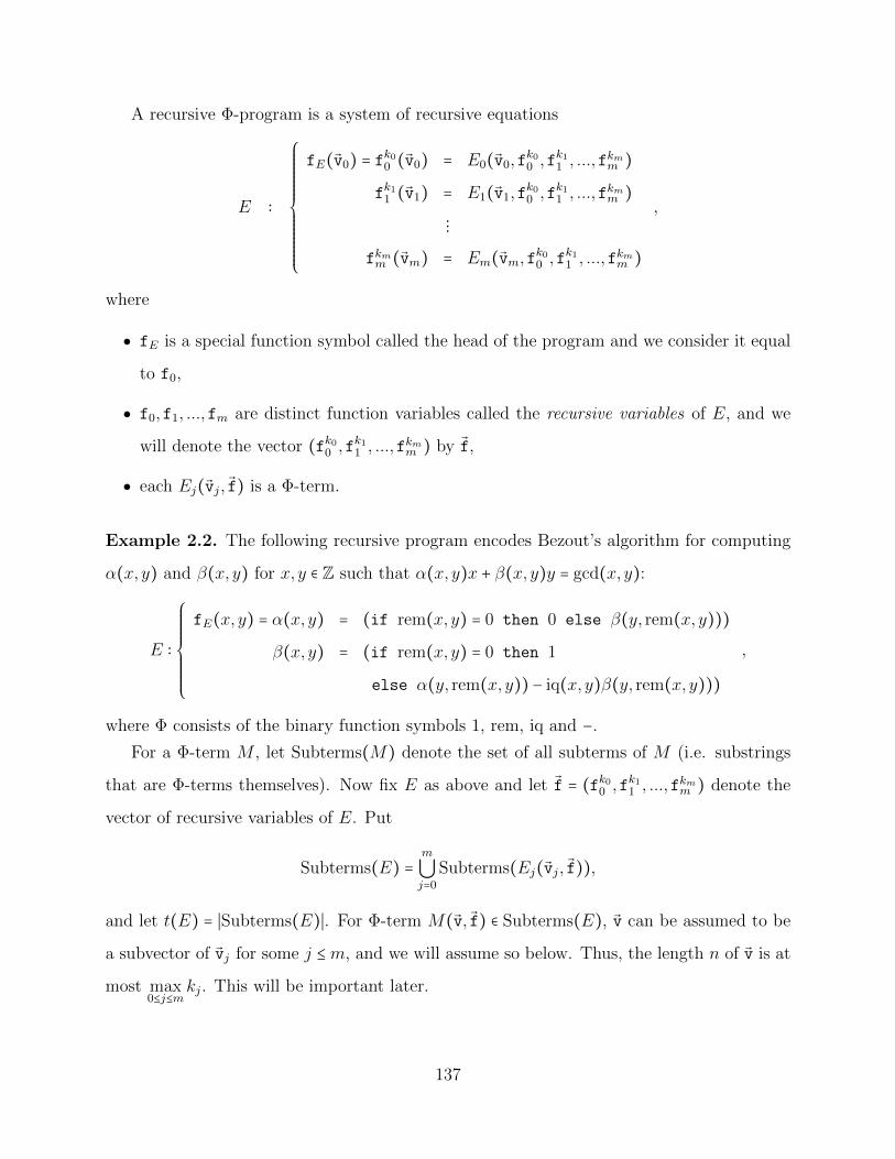
A recursive Φ-program is a system of recursive equations
E ∶
⎧⎪⎪⎪⎪⎪⎪⎪⎪⎪⎪⎪⎨⎪⎪⎪⎪⎪⎪⎪⎪⎪⎪⎪⎩
fE(v0) = fk00 (v0) = E0(v0,f
k00 ,f
k11 , ...,f
kmm )
fk11 (v1) = E1(v1,f
k00 ,f
k11 , ...,f
kmm )
⋮
fkmm (vm) = Em(vm,fk00 ,f
k11 , ...,f
kmm )
,
where
● fE is a special function symbol called the head of the program and we consider it equal
to f0,
● f0,f1, ...,fm are distinct function variables called the recursive variables of E, and we
will denote the vector (fk00 ,f
k11 , ...,f
kmm ) by f,
● each Ej(vj, f) is a Φ-term.
Example 2.2. The following recursive program encodes Bezout’s algorithm for computing
α(x, y) and β(x, y) for x, y ∈ Z such that α(x, y)x + β(x, y)y = gcd(x, y):
E ∶
⎧⎪⎪⎪⎪⎪⎪⎪⎨⎪⎪⎪⎪⎪⎪⎪⎩
fE(x, y) = α(x, y) = (if rem(x, y) = 0 then 0 else β(y, rem(x, y)))
β(x, y) = (if rem(x, y) = 0 then 1
else α(y, rem(x, y)) − iq(x, y)β(y, rem(x, y)))
,
where Φ consists of the binary function symbols 1, rem, iq and −.
For a Φ-term M , let Subterms(M) denote the set of all subterms of M (i.e. substrings
that are Φ-terms themselves). Now fix E as above and let f = (fk00 ,f
k11 , ...,f
kmm ) denote the
vector of recursive variables of E. Put
Subterms(E) =m
⋃j=0
Subterms(Ej(vj, f)),
and let t(E) = ∣Subterms(E)∣. For Φ-term M(v, f) ∈ Subterms(E), v can be assumed to be
a subvector of vj for some j ≤m, and we will assume so below. Thus, the length n of v is at
most max0≤j≤m
kj. This will be important later.
137
2.2 Semantics
Definition 2.3. Given a signature Φ consisting of function symbols, a Φ-algebra is a struc-
ture A = (A,0A,{φA}φ∈Φ) in the signature (0,Φ) that interprets 0 as an element 0A ∈ A and
every φ ∈ Φ as a partial function φA ∶ A⇀ A.
We refer to the functions in ΦA as the primitives of the Φ-algebra A.
We now define interpretation of Φ-terms. For a Φ-term M(v,fk00 ,f
k11 , ...,f
kmm ), where
v = (v1, ...,vn), and a structure A = (A,0A,{φA}φ∈Φ). Then the interpretation of M by A is
a partial function (map)
MA ∶ An ×Partial(Ak0 ,A) ×Partial(Ak1 ,A) × ... ×Partial(Akm ,A)→ A
defined in the usual way by recursion on the complexity of M : we will spare the reader the
rigorous definition as it is enough say that MA(a, f0, f1, ..., fm) is the value one obtains when
substituting v with a and fkjj with fj in M(v,fk0
0 ,fk11 , ...,f
kmm ), for a ∈ An, fj ∈ Partial(Akj ,A)
and j ≤m.
We also define a functional
FAM ∶ Partial(Ak0 ,A) ×Partial(Ak1 ,A) × ... ×Partial(Akm ,A)⇀ Partial(An,A)
by setting
FAM(f0, f1, ..., fm) =MA( ⋅ , f0, f1, ..., fm),
for fj ∈ Partial(Akj ,A), j ≤m.
Intuitively, it is clear that a Φ-program E defines a partial function, whose domain is the
set of inputs on which E halts. Here we give a rigorous definition of this. Given a program
E as above and a Φ-algebra A, define a system of recursive equations:
⎧⎪⎪⎪⎪⎪⎪⎪⎪⎪⎪⎪⎨⎪⎪⎪⎪⎪⎪⎪⎪⎪⎪⎪⎩
f0 = FAE0
(f0, f1, ..., fm)
f1 = FAE1
(f0, f1, ..., fm)
⋮
fm = FAEm
(f0, f1, ..., fm)
,
138
a solution to which is a tuple
(f0, f1, ..., fm) ∈ Partial(Ak0 ,A) ×Partial(Ak1 ,A) × ... ×Partial(Akm ,A).
By Lemma 1B.1 (the Fixed Point Lemma) of [Mos], this system has a least (with respect
to inclusion of partial functions) solution f∗ = (f∗0 , f∗1 , ..., f∗m) since the functionals FAEj
are
monotone and continuous. We declare f∗0 the partial function that E computes with respect
to the Φ-algebra A, and we denote it by fAE . For a ∈ Ak0 , we write EA(a) ↓ to mean that
fAE(a) ↓.
Fix E and A as above and let f = (fk00 ,f
k11 , ...,f
kmm ) denote the vector of recursive variables
of E. Given a M(v, f) ∈ Subterms(E) and a ∈ An, we call the term M(a, f), obtained by
substituting v with a, an (A,E)-term. We say that an (A,E)-term M =M(a, f) converges
(or is convergent) if MA(a, f∗) ↓, where f∗ is as above. We denote the value MA(a, f∗) ∈ A
by MAE (or just M , if A and E are understood). Finally, we denote the set of all convergent
(A,E)-terms by Conv(A,E).For an (A,E)-term M =M(a, f), a = (a1, ..., an) ∈ An, we call a1, ..., an the parameters of
M and denote Param(M) = {a1, ..., an}. We also put Param0(M) = Param(M) ∪ {0A}. For
a subset B ⊆ A, we say that M is a (B,E)-term if Param0(M) ⊆ B.
3 Computation tree
For a set X and u, v ∈X<∞ ∖ {∅}, we say that u is below v, and write u ⪯ v, if u is an initial
segment of v; that is, v = (v1, v2, ..., vl) and u = (v1, v2, ..., vm) for some m ≤ l (note that
l,m ≥ 1). A tree T on a set X is a subset of X<∞ ∖ {∅} that is closed downward, i.e. for all
u, v ∈X<∞ ∖ {∅}, v ∈ T ∧ u ⪯ v implies u ∈ T . For a tree T on X and x ∈X, we put
x⌢T = {(x)} ∪ {(x,x1, ..., xl) ∈X<∞ ∶ (x1, ..., xl) ∈ T}.
Also, for finite T , we define its depth depth(T ) by setting
depth(T ) = max{∣u∣ ∶ u ∈ T} − 1,
where ∣u∣ denotes the length of u, i.e. for u ∈X l, ∣u∣ = l.
139
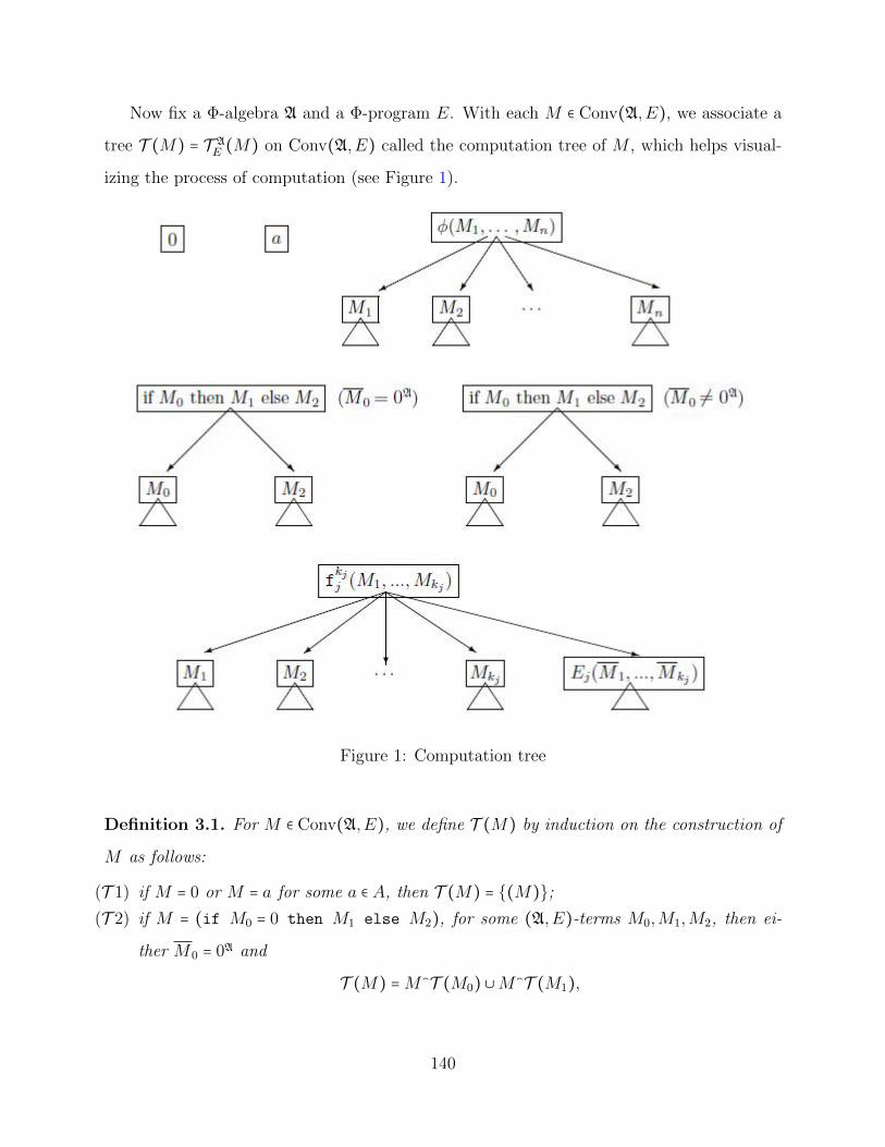
Now fix a Φ-algebra A and a Φ-program E. With each M ∈ Conv(A,E), we associate a
tree T (M) = T AE (M) on Conv(A,E) called the computation tree of M , which helps visual-
izing the process of computation (see Figure 1).
Figure 1: Computation tree
Definition 3.1. For M ∈ Conv(A,E), we define T (M) by induction on the construction of
M as follows:
(T 1) if M = 0 or M = a for some a ∈ A, then T (M) = {(M)};
(T 2) if M = (if M0 = 0 then M1 else M2), for some (A,E)-terms M0,M1,M2, then ei-
ther M0 = 0A and
T (M) =M⌢T (M0) ∪M⌢T (M1),
140
or else M0 ≠ 0A and
T (M) =M⌢T (M0) ∪M⌢T (M2);
(T 3) if M = φ(M1, ...,Mn), then T (M) = ⋃ni=1M⌢T (Mi);
(T 4) if M = fkjj (M1, ...,Mkj), then
T (M) =kj
⋃i=1
M⌢T (Mi) ∪M⌢T (Ej(M1, ...,Mkj)).
We say that an (A,E)-term N is in T (M) if (N1, ...,Nl,N) ∈ T (M) for some (A,E)-terms
N1, ...,Nl, where l can be 0.
4 Complexity measures
In this section we define various complexity measures of convergent (A,E)-terms, for fixed
Φ-algebra A and a Φ-program E.
4.1 Tree-depth complexity
For a convergent (A,E)-term M , T (M) is finite, and we define the tree-depth complexity
D(M) =D(A,E)(M) of M as the depth of T (M):
D(M) =D(A,E)(M) = depth(T (M)).
We also define the tree-depth complexity d(A,E)(a) of the program E on input a ∈ FAE by
d(A,E)(a) =D(fE(a)).
This complexity measure is not of practical importance as in (T 4) of Definition 3.1 it
corresponds to the complexity of an unrealistic parallel computation, where the input of a
function is computed in parallel to the computation of the function on that input. However,
it is a useful tool for analyzing various properties of recursive programs, and the following
is a simple example of its use.
Definition 4.1. For a program E, we define its total arity a = a(E) as the maximum of the
arities of its recursive variables and function symbols in Φ. That is:
a = a(E) = max{max1≤j≤m
kj,maxφ∈Φ
arity(φ)}.
141
Note that a(E) ≥ 1 and each node in T (M) has at most a(E) + 1 successors. Thus,
denoting by ∣T (M)∣ the cardinality (number of nodes) of T (M), we immediately get:
Proposition 4.2. For all M ∈ Conv(A,E), ∣T (M)∣ ≤ (a(E) + 1)D(M).
4.2 Sequential logical complexity
For M ∈ Conv(A,E), we define its sequential logical complexity Ls (M) = L
s
(A,E)(M) by
induction on the construction of M as follows:
(Ls1) if M = 0 or M = a for some a ∈ A, then L
s (M) = 0;
(Ls2) if M = (if M0 = 0 then M1 else M2), for some (A,E)-terms M0,M1,M2, then
either M0 = 0A and
Ls (M) = 1 +Ls (M0) +L
s (M1),
or else M0 ≠ 0A and
Ls (M) = 1 +Ls (M0) +L
s (M2);
(Ls3) if M = φ(M1, ...,Mn), then L
s (M) = 1 +∑ni=1L
s (Mi);
(Ls4) if M = f
kjj (M1, ...,Mkj), then
Ls (M) = 1 +
kj
∑i=1
Ls (Mi) +L
s (Ej(M1, ...,Mkj)).
We also define the sequential logical complexity ls(A,E)(a) of the program E on input
a ∈ dom(fAE) by
ls(A,E)(a) = Ls (fE(a)).
This notion of complexity counts every step made by the program during the computation
without any parallelism involved. We also have:
Proposition 4.3. For all M ∈ Conv(A,E), Ls(M) ≤ ∣T (M)∣.
Proof. Straightforward induction on the construction of M .
142
4.3 Parallel logical complexity
For M ∈ Conv(A,E), we define its parallel logical complexity Lp(M) = Lp
(A,E)(M) by induc-
tion on the construction of M as follows:
(Lp1) if M = 0 or M = a for some a ∈ A, then L
p(M) = 0;
(Lp2) if M = (if M0 = 0 then M1 else M2), for some (A,E)-terms M0,M1,M2, then
either M0 = 0A and
Lp(M) = 1 +max{Lp(M0), L
p(M1)},
or else M0 ≠ 0A and
Lp(M) = 1 +max{Lp(M0), L
p(M2)};
(Lp3) if M = φ(M1, ...,Mn), then L
p(M) = 1 +max1≤i≤nLp(Mi);
(Lp4) if M = f
kjj (M1, ...,Mkj), then
Lp(M) = 1 + max
1≤i≤kjL
p(Mi) +Lp(Ej(M1, ...,Mkj)).
We also define the sequential logical complexity lp(A,E)(a) of the program E on input
a ∈ dom(fAE) by
lp(A,E)(a) = Lp(fE(a)).
This notion of complexity corresponds to the time-complexity of a realistic parallel com-
putation, and this is clear for all clauses of the above definition, except maybe for (Lp3) and
(Lp4). Here is the justification for these clauses:
For (Lp3), the question may be that how can we choose to compute M1 or M2 before
knowing whether M0 = 0A or not. It is even possible that M0 = 0A and M2 does not converge;
thus, it seems that to have a convergent computation, we have to first check whether or not
M0 = 0A, so that we know which of M1 and M2 to compute. However, we can do the
following trick: start computing M0,M1 and M2 in parallel, and go until M0 halts. Now
if M0 = 0A, stop the computation of M2 and resume the computation of M1 if it hadn’t
143
halted yet. Otherwise, stop the computation of M1 and resume the computation of M2 if it
hadn’t halted yet. In this manner, we make only max{LP (M0), LP (M1)} steps in the first
case, and max{LP (M0), LP (M2)} in the second, in addition to the step corresponding to
processing the (if . . . = 0 then . . . else . . .) operation.
The justification for (Lp4) is more straightforward: we need to first compute the input
M1,M2, ...,Mkj of the function, before computing the function. Hence, we add max1≤i≤kj Lp(Mi)
to Lp(Ej(M1, ...,Mkj)) instead of taking the maximum of the two. The additional 1 is there
to count the call of the function fkjj .
Lastly we note the following:
Proposition 4.4. For all M ∈ Conv(A,E), D(M) = depth(T (M)) ≤ Lp(M).
Proof. Straightforward induction on the construction of M .
4.4 Sequential call complexity
For M ∈ Conv(A,E), we define its sequential call complexity Cs (M) = Cs
(A,E)(M) by induc-
tion on the construction of M as follows:
(Cs1) if M = 0 or M = a for some a ∈ A, then C
s (M) = 0;
(Cs2) if M = (if M0 = 0 then M1 else M2), for some (A,E)-terms M0,M1,M2, then
either M0 = 0A and
Cs (M) = Cs (M0) +C
s (M1),
or else M0 ≠ 0A and
Cs (M) = Cs (M0) +C
s (M2);
(Cs3) if M = φ(M1, ...,Mn), then C
s (M) = 1 +∑ni=1C
s (Mi);
(Cs4) if M = f
kjj (M1, ...,Mkj), then
Cs (M) =
kj
∑i=1
Cs (Mi) +C
s (Ej(M1, ...,Mkj)).
We also define the sequential call complexity cs(A,E)(a) of the program E on input a ∈
dom(fAE) by
cs(A,E)(a) = Cs (fE(a)).
144
This complexity measure registers the number of times the program calls a primitive
(function in ΦA) during a sequential computation.
4.5 Parallel call complexity
For M ∈ Conv(A,E), we define its parallel call complexity Cp(M) = Cp
(A,E)(M) by induction
on the construction of M as follows:
(Cp1) if M = 0 or M = a for some a ∈ A, then C
p(M) = 0;
(Cp2) if M = (if M0 = 0 then M1 else M2), for some (A,E)-terms M0,M1,M2, then
either M0 = 0A and
Cp(M) = max{Cp(M0),C
p(M1)},
or else M0 ≠ 0A and
Cp(M) = max{Cp(M0),C
p(M2)};
(Cp3) if M = φ(M1, ...,Mn), then C
p(M) = 1 +max1≤i≤nCp(Mi);
(Cp4) if M = f
kjj (M1, ...,Mkj), then
Cp(M) = max
1≤i≤kjC
p(Mi) +Cp(Ej(M1, ...,Mkj)).
We also define the sequential logical complexity cp(A,E)(a) of the program E on input
a ∈ dom(fAE) by
cp(A,E)(a) = Cp(fE(a)).
This complexity measure counts the maximum number of times the program calls a
primitive function during a parallel computation in the sense of the discussion in the end of
Subsection 4.3.
145
CHAPTER II
Inequalities and proofs
In this chapter we explore the relations between the complexity measures defined in the
previous chapter. Throughout, we fix a Φ-algebra A and a program
E ∶
⎧⎪⎪⎪⎪⎪⎪⎪⎪⎪⎪⎪⎨⎪⎪⎪⎪⎪⎪⎪⎪⎪⎪⎪⎩
fE(v0) = fk00 (v0) = E0(v0,f
k00 ,f
k11 , ...,f
kmm )
fk11 (v1) = E1(v1,f
k00 ,f
k11 , ...,f
kmm )
⋮
fkmm (vm) = Em(vm,fk00 ,f
k11 , ...,f
kmm )
,
5 The complete picture of inequalities
For a convergent (A,E)-term M , the following inequalities are obvious from the definitions:
Cs (M)
≤ ≤
Cp(M) L
s (M),
≤ ≤
Lp(M)
This part of the current thesis concerns reversing this inequalities.
Let µ, ν be complexity measures (e.g. µ = Lsand ν = Lp
). We write:
● µ ≤lin ν if there exist constants B0,B1 that depend only on the program E such that
for all Φ-algebras A and M ∈ Conv(A,E), we have
µ(M) ≤ B1ν(M) +B0.
● µ ≤exp ν if there exists a constant B that depends only on the program E such that
for all Φ-algebras A and M ∈ Conv(A,E), we have
µ(M) ≤ Bν(M).
146
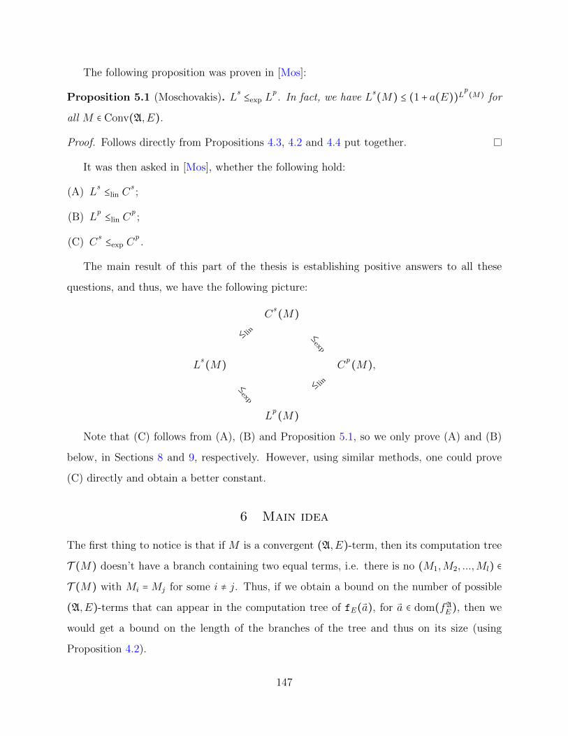
The following proposition was proven in [Mos]:
Proposition 5.1 (Moschovakis). Ls ≤exp L
p. In fact, we have L
s(M) ≤ (1+ a(E))Lp(M) for
all M ∈ Conv(A,E).
Proof. Follows directly from Propositions 4.3, 4.2 and 4.4 put together.
It was then asked in [Mos], whether the following hold:
(A) Ls ≤lin C
s;
(B) Lp ≤lin C
p;
(C) Cs ≤exp C
p.
The main result of this part of the thesis is establishing positive answers to all these
questions, and thus, we have the following picture:
Cs (M)
≤ lin ≤exp
Ls (M) C
p(M),
≤exp
≤ lin
Lp(M)
Note that (C) follows from (A), (B) and Proposition 5.1, so we only prove (A) and (B)
below, in Sections 8 and 9, respectively. However, using similar methods, one could prove
(C) directly and obtain a better constant.
6 Main idea
The first thing to notice is that if M is a convergent (A,E)-term, then its computation tree
T (M) doesn’t have a branch containing two equal terms, i.e. there is no (M1,M2, ...,Ml) ∈
T (M) with Mi =Mj for some i ≠ j. Thus, if we obtain a bound on the number of possible
(A,E)-terms that can appear in the computation tree of fE(a), for a ∈ dom(fAE), then we
would get a bound on the length of the branches of the tree and thus on its size (using
Proposition 4.2).
147
How do we find a bound on the number of possible (A,E)-terms that can appear in
T (fE(a))? Here we give an outline of how.
Lemma 6.1. For a finite subset B ⊆ A, there are at most t(E) ⋅ ∣B∣a(E)-many (B,E)-terms.
Proof. Each M ∈ Subterms(E) uses at most a(E) variables. Thus, substituting these vari-
ables with elements from B, we obtain ∣B∣a(E)-many (B,E)-terms.
In light of this lemma, we put
H =H(E) = t(E)(a(E) + 1)a(E). (6.2)
The letter H stands for height (calling this constant height is justified by Lemma 7.2 below).
For a ∈ dom(fAE), the computation of fA
E on a starts with processing the (A,E)-term
M = E0(a, f). Setting B = Param0(fE(a)) = {ai ∶ 1 ≤ i ≤ k0} ∪ {0A}, we see that the
computation tree of M starts with (B,E)-terms and continues this way until some branch
of it hits a recursive call. By Lemma 6.1, the length of the branches containing only (B,E)-
terms is at most
t(E) ⋅ (k0 + 1)a(E) ≤H.
How do new elements of A enter the computation?
Lemma 6.3. If M ∈ Conv(A,E) and Cp(M) = 0 (equivalently C
s(M) = 0), then M ∈
Param0(M).
Proof. Straightforward induction on the construction of M .
This lemma says that during the computation, we only obtain new elements of A by call-
ing a primitive φ ∈ Φ, and these new elements enter the computation tree via a recursive call.
We isolate certain (A,E)-terms that correspond to this situation (called splitting below),
and bounding the number of these terms is how we prove the desired inequalities.
7 Splitting
Definition 7.1. An (A,E)-term M is called splitting if M = fkjj (M1, ...,Mkj), for some j ≤m
and (A,E)-terms M1, ...,Mkj such that max1≤kj Cs(Mi) > 0 and C
s(Ej(M1, ...,Mkj)) > 0.
148
In this definition, we can replace Cs
with Cp
as one being nonzero is equivalent to the
other being nonzero.
For M ∈ Conv(A,E), we isolate the part of its computation tree that does not involve a
splitting term; that is:
T ′(M) = {(M1, ...,Ml) ∈ T (M) ∶ ∀i,1 ≤ i ≤ l(Mi is not splitting)}.
The following lemma shows that the computation can only make a constant (depending
only on E) number of steps before it has to encounter a splitting term:
Lemma 7.2. For M =M1 ∈ Conv(A,E), if (M1, ...,Ml) ∈ T ′(M), then l ≤ 2H. In particular,
the depth of T ′(M) is at most 2H − 1.
Proof. Since M converges, M1, ...,Ml are distinct. Put B = Param0(M). If all of Mi are
(B,E)-terms, then we are done since ∣B∣ ≤ 1+ a(E) and thus, by Lemma 6.1, the number of
distinct (B,E)-terms is bounded above by H.
Otherwise, let n < l be the least number such that Mn+1 is not a (B,E)-term; by Lemma
6.1 again,
n ≤H. (∗)
Since Mn+1 is not a (B,E)-term, it must be that Mn = fkjj (N1, ...,Nkj) and Mn+1 =
Ej(N1, ...,Nkj), for some j ≤m and (A,E)-termsN1, ...,Nkj . By the choice of n, {N1, ...,Nkj} ⊈
B, and thus, Lemma 6.3 implies:kj
∑i=1
Cs (Ni) > 0.
But Mn is not splitting, so it must be that
Cs (Mn+1) = C
s (Ej(N1, ...,Nkj)) = 0.
Hence, by Lemma 6.3, all of Mn+1, ...,Ml are (B′,E)-terms, where B′ = Param0(Mn+1).
Thus, by Lemma 6.1,
l − n ≤ t(E) ⋅ ∣B′∣a(E) ≤ t(E) ⋅ (a(E) + 1)a(E) =H.
This and (∗) together imply l ≤ 2H.
149
Put
V = V (E) = (a(E) + 1)2H , (7.3)
and, for a convergent (A,E)-term M , put
v(M) = ∣T ′(M)∣.
The above lemma implies:
Corollary 7.4. v(M) ≤ V .
8 Sequential logical vs. sequential call complexities
We now define an auxiliary complexity measure that makes the exposition of the proof of
Theorem 8.5 conceptually clear.
Definition 8.1. For M ∈ Conv(A,E), we define its sequential splitting complexity Ss(M) =
Ss
(A,E)(M) as the number of splitting terms in T (M).
Lemma 8.2. For all M ∈ Conv(A,E), Ss(M) ≤ Cs(M) � 1.
Proof. The proof is by induction on the construction of M as usual, and we only write it for
the case when M is splitting as Ss (M) does not increase in other cases. So suppose that
M = fkjj (M1, ...,Mkj) for some j ≤m and M is splitting. Then
kj
∑i=1
Cs (Mi) > 0 and C
s (Ej(M1, ...,Mkj)) > 0.
Hence, by induction, we have
Ss (M) = 1 +
kj
∑i=1
Ss (Mi) + S
s (Ej(M1, ...,Mkj))
≤ 1 + (kj
∑i=1
Cs (Mi) − 1) + (Cs (Ej(M1, ...,Mkj)) − 1)
=kj
∑i=1
Cs (Mi) +C
s (Ej(M1, ...,Mkj)) − 1
= Cs (M) − 1.
150
Lemma 8.3. If M ∈ Conv(A,E), then there is a (possibly empty) sequence of splitting terms
N0, ...,Nl−1 in T (M) such that
Ss(M) =∑
i<lS
s(Ni) and Ls(M) ≤∑
i<lL
s(Ni) + v(M).
Proof. We prove by induction on the construction of M as usual. If M itself is splitting, just
take N0 =M . If there are no splitting nodes in T (M), then T ′(M) = T (M), and the lemma
trivially holds by taking l = 0 and using Lemma 4.3. The rest of the cases (T 2), (T 3), and
(T 4) of Definition 3.1 are handled in the same manner, and we only write the proof for case
(T 4) for a non-splitting M . So suppose M is non-splitting and
M = fkjj (M1, ...,Mkj).
Put l = kj + 1 and Ml = Ej(M1, ...,Mkj). By the induction hypothesis, there are splitting
terms N i1, ...,N
ini
in T (M) such that
Ss (M) = ∑
1≤i≤lS
s (Mi) = ∑1≤i≤l
1≤p≤ni
Ss (N i
p),
and also
Ls (M) = 1 + ∑
1≤i≤lL
s (Mi)
≤ 1 + ∑1≤i≤l
( ∑1≤p≤ni
Ls (N i
p) + v(Mi))
= ∑1≤i≤l
1≤p≤ni
Ls (N i
p) + 1 + ∑1≤i≤l
v(Mi)
= ∑1≤i≤l
1≤p≤ni
Ls (N i
p) + v(M).
We are finally ready to prove the main lemma.
Lemma 8.4. For every M ∈ Conv(A,E), we have:
(a) If M is splitting, then Ls(M) ≤ ((a + 1)V + 1) ⋅ Ss(M);
(b) If M is not splitting, then Ls(M) ≤ ((a + 1)V + 1) ⋅ Ss(M) + V ;
151
where a = a(E) and V = V (E).
Proof. We prove (a) and (b) together by induction on the construction of M , noting that (b)
is a weaker inequality than (a) and so we can use it when we invoke the induction hypothesis
regardless of whether M is splitting or not.
Case 1 : .M is splitting. Then M = fkjj (M1, ...,Mkj). Set l = kj +1 and Ml = Ej(M1, ...,Mkj).
By the definition of a = a(E), l ≤ a + 1. Thus, using the induction hypothesis, we compute:
Ls (M) = Ls (M1) + ... +L
s (Ml) + 1
≤ ((a + 1)V + 1) ⋅ [Ss (M1) + ... + Ss (Ml)] + (lV + 1)
≤ ((a + 1)V + 1) ⋅ [Ss (M1) + ... + Ss (Ml)] + ((a + 1)V + 1)
= ((a + 1)V + 1) ⋅ [Ss (M1) + ... + Ss (Ml) + 1]
= ((a + 1)V + 1) ⋅ Ss (M).
Case 2 : .M is not splitting. Then, by Lemma 8.3, there are splitting terms N0, ...,Nl−1 in
T (M) such that
Ss (M) =∑
i<lS
s (Ni) and Ls (M) ≤∑
i<lL
s (Ni) + v(M).
Thus, using Corollary 7.4 and the induction hypothesis, we compute:
Ls (M) ≤ Ls (N1) + ... +L
s (Nl) + v(M)
≤ ((a + 1)V + 1) ⋅ [Ss (N1) + ... + Ss (Nl)] + v(M)
≤ ((a + 1)V + 1) ⋅ Ss (M) + V.
Theorem 8.5. For every Φ-program E, Ls ≤lin C
s. In particular, there exists constants
B0,B1 depending on E such that for every Φ-algebra A and every a ∈ dom(fAE), we have:
ls(A,E)(a) ≤ B1 ⋅ cs(A,E)(a) +B0.
Proof. Follows from Lemmas 8.4 and 8.2 by taking B0 = V (E) and B1 = (a(E) + 1)V (E) + 1.
152
9 Parallel logical vs. parallel call complexities
In this section, we obtain the analogue of Theorem 8.5 for Lp
and Cp. The proof follows the
same outline as in the previous section.
Definition 9.1. For M ∈ Conv(A,E), we define its parallel splitting complexity Sp(M) =
Sp
(A,E)(M) by induction on the construction of M as follows:
(Sp1) if M = 0 or M = a for some a ∈ A, then S
p(M) = 0;
(Sp2) if M = (if M0 = 0 then M1 else M2), for some (A,E)-terms M0,M1,M2,
then either M0 = 0A and
Sp(M) = max{Sp(M0), S
p(M1)},
or else M0 ≠ 0A and
Sp(M) = max{Sp(M0), S
p(M2)};
(Sp3) if M = φ(M1, ...,Mn), then S
p(M) = max1≤i≤n Sp(Mi);
(Sp4) if M = f
kjj (M1, ...,Mkj), then either M is not splitting and
Sp(M) = max
1≤i≤kjS
p(Mi) + Sp(Ej(M1, ...,Mkj)),
or else M is splitting and
Sp(M) = 1 + max
1≤i≤kjS
p(Mi) + Sp(Ej(M1, ...,Mkj)).
Lemma 9.2. For all M ∈ Conv(A,E), Sp(M) ≤ Cp(M) � 1.
Proof. The proof is by induction on the construction of M as usual, and we only write it for
the case when M is splitting as Sp(M) does not increase in other cases. So suppose that
M = fkjj (M1, ...,Mkj) for some j ≤m and M is splitting. Then
max1≤i≤kj
Cp(Mi) > 0 and C
p(Ej(M1, ...,Mkj)) > 0.
153
Hence, by induction, we have
Sp(M) = 1 +
kjmaxi=1
Sp(Mi) + S
p(Ej(M1, ...,Mkj))
≤ 1 + (kj
maxi=1
Cp(Mi) − 1) + (Cp(Ej(M1, ...,Mkj)) − 1)
=kj
maxi=1
Cp(Mi) +C
p(Ej(M1, ...,Mkj)) − 1
= Cp(M) − 1.
Definition 9.3. Call an (A,E)-term M a leaf if M = 0 or M = a for some a ∈ A.
Lemma 9.4. If M ∈ Conv(A,E), then there is an (A,E)-term N in T (M) that is either a
leaf or splitting and is such that
Lp(M) ≤ Lp(N) + v(M).
Proof. We prove by induction on the construction of M as usual. If M itself is a leaf or
splitting, then take N =M . Otherwise, we consider cases:
Case 1 : .M = φ(M1, ...,Mn). Then Lp(M) = Lp(Mi) + 1 for some i, 1 ≤ i ≤ n, and the
induction hypothesis gives us a leaf or splitting term N in T (Mi) such that
Lp(Mi) ≤ Lp(N) + v(Mi).
Since M is not splitting,
T ′(M) =n
⋃i=1
M⌢T ′(M)
and so v(M) ≥ v(Mi) + 1. Thus, it follows that
Lp(M) = Lp(Mi) + 1 ≤ Lp(N) + v(Mi) + 1 ≤ Lp(N) + v(M).
Case 2 : .M = (if M0 = 0 then M1 else M2). The argument for this case is similar to
that for Case 1, so we will skip it.
Case 3 : .M is not splitting and M = fkjj (M1, ...,Mkj). Set M ′ = Ej(M1, ...,Mkj) and choose
i such that Lp(Mi) = max{Lp(M1), ..., Lp(Mkj)}.
154
If Cp(Mi) = 0, then L
p(Mi) ≤ Ls (Mi) ≤ ∣T (Mi)∣ = v(Mi) because T (M) = T ′(M). By
the induction hypothesis applied to M ′, there is an (A,E)-term N in T (M ′) that is a leaf
or splitting and is such that
Lp(M ′) ≤ Lp(N) + v(M ′).
Hence:
Lp(M) = Lp(Mi) +L
p(M ′) + 1 ≤ v(Mi) +Lp(N) + v(M ′) + 1.
Since M is not splitting, we have v(M) ≥ v(Mi) + v(M ′) + 1, so
Lp(M) ≤ Lp(N) + v(M).
If Cp(Mi) > 0, then C
p(M ′) = 0 since M is non-splitting, and we can repeat the same
argument with the roles of Mi and M ′ swapped.
Lemma 9.5. For every M ∈ Conv(A,E), we have:
(a) If M is splitting, then Lp(M) ≤ (2V + 1) ⋅ Sp(M);
(b) If M is not splitting, then Lp(M) ≤ (2V + 1) ⋅ Sp(M) + V ;
where V = V (E).
Proof. We prove (a) and (b) together by induction on the construction of M , noting that (b)
is a weaker inequality than (a) and so we can use it when we invoke the induction hypothesis
regardless of whether M is splitting or not.
Case 1 : .M is splitting. Then M = fkjj (M1, ...,Mkj). Set M ′ = Ej(M1, ...,Mkj) and compute:
Lp(M) = max
1≤i≤kjL
p(Mi) +Lp(M ′) + 1
≤ (2V + 1) ⋅ max1≤i≤kj
Sp(Mi) + V + (2V + 1) ⋅ Sp(M ′) + V + 1
= (2V + 1) ⋅ [max1≤i≤kj
Sp(Mi) + S
p(M ′) + 1]
= (2V + 1) ⋅ Sp(M).
155
Case 2 : .M is not splitting. Then, by Lemma 9.4, there is an (A,E)-term N in T (M) that
is a leaf or splitting and is such that
Lp(M) ≤ Lp(N) + v(M).
Using the obvious fact that Sp(N) ≤ Sp(M), together with Corollary 7.4 and the induction
hypothesis, we compute:
Lp(M) ≤ Lp(N) + v(M)
≤ (2V + 1) ⋅ Sp(N) + v(M)
≤ (2V + 1) ⋅ Sp(M) + V.
Theorem 9.6. For every Φ-program E, Lp ≤lin C
p. In particular, there exists constants
B0,B1 depending on E such that for every Φ-algebra A and every a ∈ dom(fAE), we have:
lp(A,E)(a) ≤ B1 ⋅ cp(A,E)(a) +B0.
Proof. Follows from Lemmas 9.5 and 9.2 by taking B0 = V (E) and B1 = 2V (E) + 1.
156
Bibliography
[Ada90] S. Adams, Trees and amenable equivalence relations, Ergodic Theory Dynamical Systems 10
(1990), 1-14.
[AS90] S. Adams and R. Spatzier, Kazhdan groups, cocycles and trees, Amer. J. Math. 112 (1990),
271-287.
[BK96] H. Becker and A. S. Kechris, The Descriptive Set Theory of Polish Group Actions, London Math.
Soc. Lecture Note Series, vol. 232, Cambridge Univ. Press, 1996.
[Coh89] D. E. Cohen, Combinatorial Group Theory: A Topological Approach, London Math. Soc. Student
Texts, vol. 14, Cambridge Univ. Press, 1989.
[DP02] A. I. Danilenko and K. K. Park, Generators and Bernoullian factors for amenable actions and
cocycles on their orbits, Ergodic Theory and Dynamical Systems 22 (2002), 1715-1745.
[DJK94] R. Dougherty, S. Jackson, and A. S. Kechris, The Structure of Hyperfinite Borel Equivalence
Relations, Trans. of the Amer. Math. Soc. 341 (1994), no. 1, 193-225.
[Dow11] T. Downarowicz, Entropy in Dynamical Systems, New Mathematical Monographs Series, vol. 18,
Cambridge Univ. Press, 2011.
[Dye63] H. A. Dye, On groups of measure preserving transformations, Amer. J. Math. 85 (1963), 551-576.
[EHN93] S. Eigen, A. Hajian, and M. Nadkarni, Weakly wandering sets and compressibility in a descriptive
setting, Proc. Indian Acad. Sci. 103 (1993), no. 3, 321-327.
[EW11] M. Einsiedler and T. Ward, Ergodic Theory with a View Towards Number Theory, Graduate Texts
in Mathematics, vol. 259, Springer, 2011.
[Far62] R. H. Farrell, Representation of invariant measures, Illinois J. Math. 6 (1962), 447-467.
[FM77] J. Feldman and C. C. Moore, Ergodic equivalence relations and von Neumann algebras, I. Trans.
Amer. Math. Soc. 234 (1977), 289-324.
[GJ12] S. Gao and S. Jackson, Countable abelian group actions and hyperfinite equivalence relations, To
appear in Inventiones Mathematicae (2012).
[Gla03] E. Glasner, Ergodic Theory via Joinings, Mathematical Surveys and Monographs, vol. 101, Amer-
ican Mathematical Society, 2003.
[GW02] E. Glasner and B. Weiss, Minimal actions of the group S(Z) of permutations of the integers,
Geom. Funct. Anal. 12 (2002), 964-988.
157
[HI69] A. B. Hajian and Y. Ito, Weakly wandering sets and invariant measures for a group of transfor-
mations, Journal of Math. Mech. 18 (1969), 1203-1216.
[HK64] A. B. Hajian and S. Kakutani, Weakly wandering sets and invariant measures, Trans. Amer.
Math. Soc. 110 (1964), 136-151.
[HKL90] L. A. Harrington, A. S. Kechris, and A. Louveau, A Glimm-Effros dichotomy for Borel equivalence
relations, Journal of the Amer. Math. Soc. 3 (1990), no. 4, 903-928.
[Hjo02] G. Hjorth, A lemma for cost attained, Annals of Pure and Applied Logic 143 (2002), no. 16,
87-102.
[JKL02] S. Jackson, A. S. Kechris, and A. Louveau, Countable Borel equivalence relations, Journal of
Math. Logic 2 (2002), no. 1, 1-80.
[Kec95] A. S. Kechris, Classical Descriptive Set Theory, Graduate Texts in Mathematics, vol. 156,
Springer, 1995.
[KM04] A. S. Kechris and B. Miller, Topics in Orbit Equivalence, Lecture Notes in Math., vol. 1852,
Springer, 2004.
[Kre70] U. Krengel, Transformations without finite invariant measure have finite strong generators, First
Midwest Conference, Ergodic Theory and Probability, Springer Lecture Notes, vol. 160, 1970,
pp. 133-157.
[Kri69] W. Krieger, On non-singular transformations of a measure space, Z. Wahrschein. veew. Geb. 11
(1969), 98-119.
[Kri70] W. Krieger, On entropy and generators of measure-preserving transformations, Trans. Amer.
Math. Soc. 149 (1970), 453-464.
[Kun74] A. J. Kuntz, Groups of transformations without finite invariant measures have strong generators
of size 2, Annals of Probability 2 (1974), no. 1, 143-146.
[LM92] A. Lubotzky and Sh. Mozes, Asymptotic properties of unitary representations of tree automor-
phisms, Harmonic analysis and discrete potential theory (1992), 289-298.
[Mar13] A. Marks, A determinacy approach to Borel combinatorics, Submitted (2013), available at http:
//www.its.caltech.edu/~marks/.
[McC63] J. McCarthy, A basis for a mathematical theory of computation, Computer programming and
formal systems (1963), 33-70.
158
[Mil04] B. D. Miller, PhD Thesis: Full groups, classification, and equivalence relations, University of
California at Los Angeles, 2004.
[Mil08] B. D. Miller, The existence of measures of a given cocycle, II: Probability measures, Ergodic
Theory and Dynamical Systems 28 (2008), no. 5, 1615-1633.
[Mos] Y. N. Moschovakis, Recursion and Complexity, Unpublished Lecture Notes.
[MvdD04] Y. N. Moschovakis and L. van den Dries, Is the Euclidean algorithm optimal among its peers?,
The Bulletin of Symbolic Logic 10 (2004), no. 3, 390-418.
[MvdD09] Y. N. Moschovakis and L. van den Dries, Arithmetic complexity, ACM Trans. on Computational
Logic 10 (2009), no. 2, 1-49.
[Mun53] M. E. Munroe, Introduction to Measure and Integration, Addison-Wesley, 1953.
[Nad91] M. G. Nadkarni, On the existence of a finite invariant measure, Proc. Indian Acad. Sci. Math.
Sci. 100 (1991), 203-220.
[OW80] D. Ornstein and B. Weiss, Ergodic theory and amenable group actions, I: The Rohlin lemma.,
Bull. Amer. Math. Soc. 2 (1980), 161-164.
[Rud90] D. Rudolph, Fundamentals of Measurable Dynamics, Oxford Univ. Press, 1990.
[Tho09] S. Thomas, Continuous vs. Borel reductions, accepted for publication in Arch. Math. Logic (2009).
[TW13] S. Thomas and J. Williams, The bi-embeddability relation for finitely generated groups, accepted
for publication in J. of London Math. Soc. (2013).
[Var63] V. S. Varadarajan, Groups of automorphisms of Borel spaces, Trans. Amer. Math. Soc. 109
(1963), 191-220.
[Wag93] S. Wagon, The Banach-Tarski Paradox, Cambridge Univ. Press, 1993.
[Wei84] B. Weiss, Measurable dynamics, Contemp. Math. 26 (1984), 395-421.
[Wei87] B. Weiss, Countable generators in dynamics-universal minimal models, Measure and Measurable
Dynamics, Contemp. Math. 94 (1987), 321-326.
159
![Finite categoricity and[10mm] Non-atomicity of free algebrasmathematics.ceu.edu/.../basicpage/27/etdthesis1.pdf · By Morley’s categoricity theorem, a countable, first order theory](https://img.dokumen.tips/doc/110x75/5f0d0a4e7e708231d43861a1/finite-categoricity-and10mm-non-atomicity-of-free-by-morleyas-categoricity-theorem.jpg)