Embed Size (px)
Citation preview

Chapter 8: Anthropogenic and Natural
Radiative Forcing Presented by
Ken Sinclair
March 14th 2014

Overview Chapter 8
8.1 Radiative Forcing 8.2 Atmospheric Chemistry 8.3 Present-Day Anthropogenic Radiative Forcing 8.4 Natural Radiative Forcing Changes: Solar and Volcanic 8.5 Synthesis of Global Mean Radiative Forcing, Past and Future 8.6 Geographic Distribution of Radiative Forcing 8.7 Emission Metrics

Radiative Forcing 8.1 Box 8.1 | Definition of Radiative Forcing and Effective Radiative Forcing
AR5 uses the previously used Radiative Forcing (RF) concept and introduces Effective Radiative Forcing (ERF)
RF is defined, as it was in AR4, as the change in net downward radiative flux at the tropopause after allowing for stratospheric temperatures to readjust to radiative equilibrium, while holding surface and tropospheric temperatures and state variables such as water vapor and cloud cover fixed at the unperturbed values.
ERF is the change in net TOA downward radiative flux after allowing for atmospheric temperatures, water vapour and clouds to adjust, but with surface temperature or a portion of surface conditions unchanged. • There are multiple methods to calculate ERF, we take ERF to mean the method in which sea surface temperatures and sea ice cover are fixed at climatological values. • Land surface properties (temperature, snow and ice cover and vegetation) are allowed to adjust in this method.

Radiative Forcing 8.1 Fig. 8.1
Cartoon comparing (a) instantaneous RF, (b) RF, which allows stratospheric temperature to adjust, (c) flux change when the surface temperature is fixed over the whole Earth (a method of calculating ERF), (d) the ERF calculated allowing atmospheric and land temperature to adjust while ocean conditions are fixed and (e) the equilibrium response to the climate forcing agent. The methodology for calculation of each type of forcing is also outlined. ΔTo represents the land temperature response, while ΔTs is the full surface temperature response. (Updated from Hansen et al., 2005.)

Atmospheric Chemistry 8.2 Fig. 8.2 Time evolution of global anthropogenic and biomass burning emissions 1850–2100 used in CMIP5/ACCMIP following each Representative Concentration Pathway (RCP) • In all CMIP5/ACCMIP chemistry simulations, anthropogenic and biomass burning emissions are specified. More specifically, a single set of historical anthropogenic and biomass burning emissions (Lamarque et al., 2010) and one set of emissions for each of the RCPs (van Vuuren et al., 2011) was defined. • This was designed to increase the comparability of simulations. • These uniform emission specifications mask the existing uncertainty, so that there is in fact a considerable range in the estimates and time evolution of recent anthropogenic emissions. • Historical reconstructions of biomass burning (wildfires and deforestation) also exhibit quite large uncertainties. • In addition, the RCP biomass burning projections do not include the feedback between climate change and fires.

Atmospheric Chemistry 8.2 Fig. 8.3 Comparisons between observations and simulations for the monthly mean ozone for ACCMIP results. Correlation is indicated by the r, mean normalized bias estimated is indicated by mnbe value. • The ACCMIP model simulations indicate 10 to 20% negative bias at 250 hPa in the SH tropical region, and a slight underestimate in NH tropical region. • Comparison with satellite-based estimates of tropospheric ozone column indicates an annual mean bias of –4.3 ± 29 Tg (with a spatial correlation of 0.87 ± 0.07, 1-σ) for the ACCMIP simulations • Evaluation of simulated trends in surface ozone against observations at remote surface sites indicates an underestimation, especially in the NH. • Overall, our ability to simulate tropospheric ozone burden for present (about 2000) has not substantially changed since AR4.

Atmospheric Chemistry 8.2 Fig. 8.4
Time evolution of global tropospheric ozone burden (inTg(O3)) from 1850 to 2100 from ACCMIP results, ACCENT results (2000 only), and observational estimates. The box, whiskers, line and dot show the interquartile range, full range, median and mean burdens and differences, respectively. The dashed line indicates the 2000 ACCMIP mean. • The ACCMIP results provide an estimated tropospheric ozone increase (Figure 8.4) from 1850 to 2000 of 98 ± 17 Tg (model range), similar to AR4 estimates. • Attribution simulations indicate unequivocally that anthropogenic changes in ozone precursor emissions are responsible for the increase between 1850 and present or into the future.

Atmospheric Chemistry 8.2 Fig. 8.5
Time evolution of global-averaged mixing ratio of long-lived species1850–2100 following each RCP; blue (RCP2.6), light blue (RCP4.5), orange (RCP6.0) and red (RCP8.5). • The surface mixing ratio of CH4 has increased by 150% since pre-indus- trial times (Sections 2.2.1.1.2 and 8.3.2.2), with some projections indi- cating a further doubling by 2100 (Figure 8.5). • Nitrous oxide (N2O) in 2011 has a surface concentration 19% above its 1750 level • Anthropogenic emissions represent around 30 to 45% of the present-day global total, and are mostly from agricultural and soil sources (Fowler et al., 2009) and fossil-fuel activities. • Natural emissions come mostly from microbial activity in the soil. • The main sink for N2O is through photolysis and oxidation reactions in the stratosphere..

Present-Day Anthropogenic Radiative Forcing 8.3 Fig. 8.6
• Since AR4, the RF of CO2 has increased by 0.16 W m–2 and continues the rate noted in AR4 of almost 0.3 W m–2 per decade. • As shown in Figure 8.6(d) the rate of increase in the RF from the WMGHGs over the last 15 years has been dominated by CO2. Since AR4, CO2 has accounted for more than 80% of the WMGHG RF increase. • The interannual variability in the rate of increase in the CO2 RF is due largely to variation in the natural land uptake whereas the trend is driven by increasing anthropogenic emissions

Present-Day Anthropogenic Radiative Forcing 8.3 Fig. 8.7
Time evolution of the radiative forcing from tropospheric and stratospheric ozone • There is a noticeable acceleration in the forcing after 1950 and a deceleration in the 1990s reflecting the time evolution of anthropogenic precursor emissions. • The decreases in stratospheric ozone due to anthropogenic emissions of ODSs have a positive RF in the shortwave and a negative RF in the longwave. • The net global RF from ODSs taking into account the compensating effects on ozone and their direct effects as WMGHGs is 0.18 (0.03 to 0.33) W m–2.

8.3 Fig. 8.8
Time evolution of RF due to aerosol–radiation interaction and BC on snow and ice. Uncertainty ranges (5 to 95%) for year 2010 are shown with vertical lines. Values next to the uncertainty lines are for cases where uncertainties go beyond the scale. • The total includes the RF due to aerosol–radiation interaction for six aerosol components and RF due to BC on snow and ice. • Note that time evolution for mineral dust is not included and the total RF due to aerosol–radiation interaction is estimated based on simulations of the six other aerosol components. • After 1990 the change has been small with even a weakening of the RF due to aerosol–radiation interaction, mainly due to a stronger BC RF as a result of increased emissions in East and Southeast Asia.
Present-Day Anthropogenic Radiative Forcing

Present-Day Anthropogenic Radiative Forcing 8.3 Fig. 8.9
Change in top of the atmosphere (TOA) shortwave (SW) flux (W m–2) following the change in albedo as a result of anthropogenic Land Use Change for three periods. The lower right inset shows the globally averaged impact of the surface albedo change to the TOA SW flux (left scale) as well as the corresponding RF (right scale) after normalization to the 1750 value. • Deforestation in Europe and Asia during the last millennium led to a significant regional negative forcing. Betts et al. (2007) and Goosse et al. (2006) argue that it probably contributed to the ‘Little Ice Age’, together with natural solar and volcanic activity components.. • There is still significant uncertainty in the anthropogenic land cover change, and in particular its time evolution. • Albedo changes due to land use and land cover changes exert a heterogeneous climate forcing. The surface albedo brightened on the one hand due to a shift from forest to brighter croplands, causing local cooling, but also darkened due to the re-expansion of forests to higher latitudes and increased vegetation height in snowy regions.

Natural Radiative Forcing Changes: Solar and Volcanic 8.4 Fig. 8.10
Annual average composites of measured total solar irradiance: The Active Cavity Radiometer Irradiance Monitor (ACRIM), the Physikalisch-Meteorologisches Observatorium Davos (PMOD) and the Royal Meteorological Institute of Belgium (RMIB). Total Irradiance Monitor (TIM) measurements that are also shown. • Satellite observations of total solar irradiance (TSI) changes from 1978 to 2011 show that the most recent solar cycle minimum was lower than the prior two. This very likely led to a small negative RF of –0.04 (–0.08 to 0.00) W m–2 between 1986 and 2008.
Fig. 8.11
Reconstructions of total solar irradiance since 1745; annual resolution series from Wang et al. (2005) with and without an independent change in the background level of irradiance, Krivova et al. (2010) combined with Ball et al. (2012) and 5-year time resolution series from Steinhilber et al. (2009) and Delaygue and Bard (2011). • There are relatively large discrepancies among the models. • With these considerations, we adopt this value and range for AR5. This RF is almost half of that in AR4…

Natural Radiative Forcing Changes: Solar and Volcanic 8.4 Fig. 8.12
Volcanic reconstructions of global mean aerosol optical depth (at 550 nm). Gao et al. (2008) and Crowley and Unterman (2013) are from ice core data, and end in 2000 for Gao et al. (2008) and 1996 for Crowley and Unterman (2013). Sato et al. (1993) includes data from surface and satellite observations, and has been updated through 2011. • Emissions of CO2 from volcanic eruptions since 1750 have been at least 100 times smaller than anthropogenic emissions. • There is very high confidence that industrial-era natural forcing is a small fraction of the anthropogenic forcing except for brief periods following large volcanic eruptions.

Natural Radiative Forcing Changes: Solar and Volcanic 8.4 Fig. 8.13
• (Top) Monthly mean extinction ratio (525 nm) derived from Stratospheric Aerosol and Gas Experiment (SAGE) II extinction in 1985–2005 and Cloud-Aerosol Lidar and Infrared Pathfinder Satellite Observation (CALIPSO).. • Black contours represent the extinction ratio in log-scale from 0.1 to 100. The position of each volcanic eruption occurring during the period is displayed with its first two letters on the horizontal axis, where tropical eruptions are noted in red. • (Vi*— forest fires with stratospheric aerosol injection)

Synthesis of Global Mean Radiative Forcing, Past and Future 8.5
Confidence level of the forcing mechanisms in the 4 last IPCC assessments. In the previous IPCC assessments the level of scientific understanding (LOSU) has been adopted instead of confidence level, but for comparison with previous IPCC assessments the LOSU is converted approximately to confidence level. The thickness of the bars represents the relative magnitude of the current forcing (with a minimum value for clarity of presentation). LOSU for the RF mechanisms was not available in the first IPCC Assessment (Houghton et al., 1990)… Generally the aerosol–cloud interaction is not separated into various components in AR5, hence the confidence levels for ERF due to aerosol–cloud interaction in AR5 and for RF due to aerosol–cloud interaction from previous IPCC reports are compared… Dark green is “High agreement and Robust evidence”… orange is either “Medium agreement and Limited evidence” or “Low agreement and Medium evidence”…
Fig. 8.14

Synthesis of Global Mean Radiative Forcing, Past and Future 8.5 Fig. 8.15
Bar chart for RF (hatched) and ERF (solid) for the period 1750–2011, where the total ERF is derived from Figure 8.16. Uncertainties (5 to 95% confidence range) are given for RF (dotted) and ERF (solid). • The total anthropogenic ERF estimate for 2011 is 43% higher compared to the AR4 RF estimate for the year 2005 owing to reductions in estimated forcing due to aerosols but also to continued growth in greenhouse gas RF

Synthesis of Global Mean Radiative Forcing, Past and Future 8.5 Fig. 8.16
Probability density function (PDF) of ERF due to total GHG, aerosol forcing and total anthropogenic forcing. The GHG consists of WMGHG, ozone and stratospheric water vapour. • The magnitude of the aerosol forcing is reduced relative to AR4. • Since AR4, more aerosol processes have been included in models, and differences between models and observations persist, resulting in similar uncertainty in the aerosol forcing as in AR4. Despite the large uncertainty range, there is a high confidence that aerosols have offset a substantial portion of WMGHG global mean forcing.

Synthesis of Global Mean Radiative Forcing, Past and Future 8.5 Fig. 8.17
RF bar chart for the period 1750–2011 based on emitted compounds (gases, aerosols or aerosol precursors) or other changes… Red (positive RF) and blue (negative forcing) are used for emitted components which affect few forcing agents, whereas for emitted components affecting many compounds several colours are used as indicated in the inset at the upper part the figure. The vertical bars indicate the relative uncertainty of the RF induced by each component. Their length is proportional to the thickness of the bar, that is, the full length is equal to the bar thickness for a ±50% uncertainty. The net impact of the individual contributions is shown by a diamond symbol and its uncertainty (5 to 95% confidence range) is given by the horizontal error bar… • Due to increased concentrations, RF from WMGHGs has increased by 0.20 (0.18 to 0.22) W m–2 (8%) since the AR4 estimate for the year 2005. The RF of WMGHG is 2.83 (2.54 to 3.12) W m–2.

Synthesis of Global Mean Radiative Forcing, Past and Future 8.5 Fig. 8.18
Time evolution of forcing for anthropogenic and natural forcing mechanisms. Bars with the forcing and uncertainty ranges (5 to 95% confidence range) at present are given in the right part of the figure. For aerosol the ERF due to aerosolradiation interaction and total aerosol ERF are shown. The uncertainty ranges are for present (2011 versus 1750) and are given in Table 8.6. For aerosols, only the uncertainty in the total aerosol ERF is given. For several of the forcing agents the relative uncertainty may be larger for certain time periods compared to present. See Supplementary Material Table 8.SM.8 for further information on the forcing time evolutions. Forcing numbers provided in Annex II. The total antropogenic forcing was 0.57 (0.29 to 0.85) W m–2 in 1950, 1.25 (0.64 to 1.86) W m–2 in 1980 and 2.29 (1.13 to 3.33) W m–2 in 2011.

Synthesis of Global Mean Radiative Forcing, Past and Future 8.5 Fig. 8.19
Linear trend in anthropogenic, natural and total forcing for the indicated time periods. The uncertainty ranges (5 to 95% confidence range) are combined from uncertainties in the forcing values (from Table 8.6) and the uncertainties in selection of time period.

Synthesis of Global Mean Radiative Forcing, Past and Future 8.5 Fig. 8.20
Bar chart for RF (hatched) and ERF (solid) for the period 1980–2011, where the total anthropogenic ERF are derived from Monte-Carlo simulations similar to Figure 8.16. Uncertainties (5 to 95% confidence range) are given for RF (dotted lines) and ERF (solid lines). • Compared to the whole Industrial Era the dominance of the CO2 is larger for this recent period both with respect to other WMGHG and the total anthropogenic RF. The forcing due to aerosols is rather weak leading to a very strong net positive ERF for the 1980–2011 period. • More than 40% of the total anthropogenic ERF has occurred over the 1980–2011 period with a value close to 1.0 (0.7 to 1.3) W m–2.

Synthesis of Global Mean Radiative Forcing, Past and Future 8.5 Fig. 8.21
Radiative forcing relative to 2000 due to anthropogenic composition changes based on ACCMIP models for aerosols (with aerosol ERF scaled to match the best estimate of present-day forcing) and total ozone and RCP WMGHG forcings. Ranges are one standard deviation in the ACCMIP models and assessed relative uncertainty for WMGHGs and stratospheric water vapor. Carbonaceous aerosols refer to primary carbonaceous, while SOA are secondary organic aerosols. Note that 2030 ERF for RCP2.6 was not available, and hence the total shown for that scenario is not perfectly comparable to the other total values. RFari is RF due to aerosol–radiation interaction.

Synthesis of Global Mean Radiative Forcing, Past and Future 8.5 Fig. 8.22
Global mean anthropogenic forcing with symbols indicating the times at which ACCMIP simulations were performed (solid lines with circles are net; long dashes with squares are ozone; short dashes with diamonds are aerosol; dash-dot are WMGHG; colours indicate the RCPs with red for RCP8.5, orange RCP6.0, light blue RCP4.5, and dark blue RCP2.6). RCPs 2.6, 4.5 and 6.0 net forcings at 2100 are approximate values using aerosol ERF projected for RCP8.5 (modified from Shindell et al., 2013c). Some individual components are omitted for some RCPs for visual clarity.

Geographic Distribution of Radiative Forcing 8.6 Fig. 8.23 Spatial pattern of ACCMIP models 1850 to 2000 forcings, mean values (left) and standard deviation (right) for aerosols and ozone (top tworows). Shown are the aerosol ERF (1st row, 8 models), ozone (2nd row, 11 models), total anthropogenic composition forcing (bottom left), aerosol atmospheric absorption including rapid adjustment (bottom right, 6 models).

Geographic Distribution of Radiative Forcing 8.6 Fig. 8.24
Spatial pattern of ACCMIP and 16 AeroCom models 1850 to 2000 RF due to aerosol–radiation interaction, mean values (left) and standard deviation (right). Note that different carbonaceous aerosol diagnostics are used here compared to Figure 8.23, due to available AeroCom fields. Values above are the average of the area-weighted global means, with the area weighted mean of the standard deviation of models at each point provided in parentheses.

Geographic Distribution of Radiative Forcing 8.6 Fig. 8.25
Multi-model mean RF due to aerosol–radiation interaction of all aerosols, carbonaceous aerosols, ozone, and aerosol ERF (W m–2) for the indicated times based on the ACCMIP simulations. Global area-weighted means are given in the upper right.

Geographic Distribution of Radiative Forcing 8.6 Fig. 8.26
Multi-model mean RF (W m–2) due to aerosol–radiation interaction of all anthropogenic aerosols (first and second rows) in 2030 (left) and 2100 (right) relative to 2000 for RCP2.6 (top each) and RCP8.5 (bottom each) based on the ACCMIP simulations. The seventh row shows multi-model mean ERF (W m–2) by all anthropogenic aerosols in 2030 (left) and 2100 (right) relative to 2000 for RCP8.5. Global area-weighted means are given in the upper right of each panel.

Emission Metrics 8.7 Fig. 8.27
The cause–effect chain from emissions to climate change and impacts showing how metrics can be defined to estimate responses to emissions (left) and for development of multi-component mitigation (right). The relevance of the various effects increases downwards but at the same time the uncertainty also increases. The dotted line on the left indicates that effects and impacts can be estimated directly from emissions, while the arrows on the right side indicate how these estimates can be used in development of strategies for reducing emissions.

Emission Metrics 8.7 Fig. 8.34
Net global mean temperature change by source sector after (a) 100 and (b) 20 years (for 1-year pulse emissions). • Emission metrics such as Global Warming Potential (GWP) and Global Temperature change Potential (GTP) can be used to quantify and communicate the relative and absolute contribu- tions to climate change of emissions of different substances, and of emissions from regions/countries or sources/sectors • Forcing and temperature response can also be attributed to sectors. From this perspective and with the GTP metric, a single year’s worth of current global emissions from the energy and industrial sectors have the largest contributions to global mean warming over the next approximately 50 to 100 years. Household fossil fuel and biofuel, biomass burning and on-road transportation are also relatively large contributors to warming over these time scales, while current emissions from sectors that emit large amounts of CH4 (animal husbandry, waste/landfills and agriculture) are also important over shorter time horizons (up to 20 years).

Emission Metrics 8.7 Fig. 8.28
(a) The Absolute Global Warming Potential (AGWP) is calculated by integrating the RF due to emission pulses over a chosen time horizon; for example, 20 and 100 years (vertical lines). The GWP is the ratio of AGWP for component i over AGWP for the reference gas CO2. The blue hatched field represents the integrated RF from a pulse of CO2, while the green and red fields represent example gases with 1.5 and 13 years lifetimes, respectively. (b) The Global Temperature change Potential (GTP) is based on the temperature response at a selected year after pulse emission of the same gases; e.g., 20 or 100 years (vertical lines). See Supplementary Material Section 8.SM.11 for equations for calculations of GWP and GTP.

Emission Metrics 8.7 Fig. 8.29
Development of AGWP-CO2, AGWP-CH4 and GWP-CH4 with time horizon. The yellow and blue curves show how the AGWPs changes with increasing time horizon. Because of the integrative nature the AGWP for CH4 (yellow curve) reaches a constant level after about five decades. The AGWP for CO2 continues to increase for centuries. Thus the ratio which is the GWP (black curve) falls with increasing time horizon.

Emission Metrics 8.7 Fig. 8.30
Global Temperature change Potential (GTP(t)) for CH4, nitrous oxide and BC for each year from year of emission to the time at which the temperature change target is reached. The (time-invariant) GWP100 is also shown for N2O and CH4 for comparison.

Emission Metrics 8.7 Fig. 8.31
Changes in the RE, IRF and AGWP for CO2 for 100 years from earlier IPCC Assessment Reports normalized relative to the values given in AR5. The ‘original’ values are calculated based on the methods explained or value reported in each IPCC Assessment Report. The ‘updated’ values are calculated based on the methods used in AR5, but the input values from each Assessment Report. The difference is primarily in the formula for the RE, which was updated in TAR. The different integrated IRF in TAR relates to a different parameterisation of the same IRF (WMO, 1999).
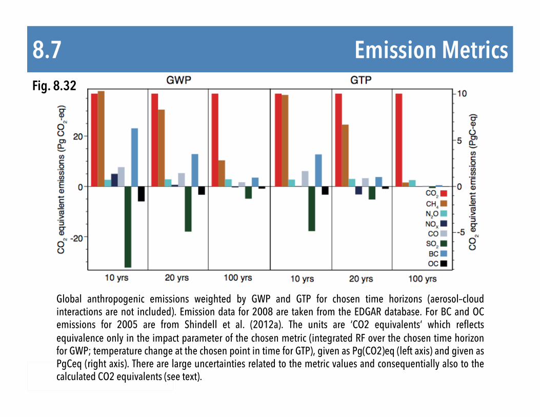
Emission Metrics 8.7 Fig. 8.32
Global anthropogenic emissions weighted by GWP and GTP for chosen time horizons (aerosol–cloud interactions are not included). Emission data for 2008 are taken from the EDGAR database. For BC and OC emissions for 2005 are from Shindell et al. (2012a). The units are ‘CO2 equivalents’ which reflects equivalence only in the impact parameter of the chosen metric (integrated RF over the chosen time horizon for GWP; temperature change at the chosen point in time for GTP), given as Pg(CO2)eq (left axis) and given as PgCeq (right axis). There are large uncertainties related to the metric values and consequentially also to the calculated CO2 equivalents (see text).

Emission Metrics 8.7 Fig. 8.33
Temperature response by component for total anthropogenic emissions for a 1-year pulse. Emission data for 2008 are taken from the EDGAR database and for BC and OC for 2005 from Shindell et al. (2012a). There are large uncertainties related to the AGTP values and consequentially also to the calculated temperature responses (see text).