Embed Size (px)
Citation preview

PAUSANIAS: Final activity report
Akrivi Vlachou, Postdoctoral Researcher
Abstract
Search engines, such as Google and Yahoo!, provide efficient retrieval and rank-ing of web pages based on queries consisting of a set of given keywords. Recentstudies show that 20% of all Web queries also have location constraints, i.e., alsorefer to the location of a geotagged web page. An increasing number of applica-tions support location-based keyword search, including Google Maps, Bing Maps,Yahoo! Local, and Yelp. Such applications depict points of interest on the mapand combine their location with the keywords provided by the associated docu-ment(s). The posed queries consist of two conditions: a set of keywords and aspatial location. The goal is to find points of interest with these keywords close tothe location. We refer to such a query as spatial-keyword query. Moreover, mobiledevices nowadays are enhanced with built-in GPS receivers, which permits appli-cations (such as search engines or yellow page services) to acquire the locationof the user implicitly, and provide location-based services. For instance, GoogleMobile App provides a simple search service for smartphones where the locationof the user is automatically captured and employed to retrieve results relevant toher current location. As an example, a search for pizza results in a list of pizzarestaurants nearby the user. In this research project, we studied how preferencequeries can be extended for supporting also keywords.
To this end we first studied preference queries in order to establish techniquesthat can be extended for supporting keywords (Chapter 1). Moreover, we proposedTop-k Spatio-Textual Preference Queries and proposed a novel indexing schemeand two algorithms for supporting efficient query processing (Chapter 2). We alsostudied the problem of maximizing the influence of spatio-textual objects basedon reverse top-k queries and keyword selection (Chapter 3). Finally, we analyzethe properties of geotagged photos of Flickr, and propose novel location-awaretag recommendation methods (Chapter 4). In summary, this research project leadto the following publications:
• George Tsatsanifos, Akrivi Vlachou: On Processing Top-k Spatio-TextualPreference Queries, in Proceedings of 18th International Conference on Ex-tending Database Technology (EDBT), Brussels, Belgium, March 23-27,2015.
• Orestis Gkorgkas, Akrivi Vlachou, Christos Doulkeridis and Kjetil Nørvag:Finding the Most Diverse Products using Preference Queries, in Proceed-ings of 18th International Conference on Extending Database Technology(EDBT), Brussels, Belgium, March 23-27, 2015.
• Ioanna Miliou, Akrivi Vlachou: Location-Aware Tag Recommendations forFlickr, DEXA (1) 2014: 97-104.
• Orestis Gkorgkas, Akrivi Vlachou, Christos Doulkeridis and Kjetil Nørvag:Efficient Processing of Exploratory Top-k Joins, in Proceedings of 26th In-ternational Conference on Scientific and Statistical Database Management(SSDBM), Aalborg, Denmark, June 30 - July 2, 2014.
• Akrivi Vlachou, Christos Doulkeridis, Kjetil Nørvag and Yannis Kotidis:Branch-and-Bound Algorithm for Reverse Top-k Queries, in Proceedings ofACM International Conference on Management of Data (SIGMOD), NewYork, USA, June 22-27, 2013.
• Orestis Gkorgkas, Akrivi Vlachou, Christos Doulkeridis and Kjetil Nørvag:Discovering Influential Data Objects over Time, in Proceedings of 13th In-ternational Symposium on Spatial and Temporal Databases (SSTD), Mu-nich, Germany, August 21-23, 2013.
• Orestis Gkorgkas, Akrivi Vlachou, Christos Doulkeridis, Kjetil Nørvag:Maximizing Influence of Spatio-Textual Objects through Keyword Selec-tion submitted for publication.
• Orestis Gkorgkas, Akrivi Vlachou, Christos Doulkeridis, Kjetil Nørvag:Exploratory product search using top-k join queries. submitted for journalpublication.
The research project is implemented within the framework of the Action Supporting Postdoctoral Researchers of theOperational Program ”Education and Lifelong Learning” (Actions Beneficiary: General Secretariat for Research andTechnology), and is co-financed by the European Social Fund (ESF) and the Greek State.

Contents
1 Preference Queries1.1 Branch-and-Bound Algorithm for Reverse Top-k Queries . . . . .1.2 Discovering Influential Data Objects over Time . . . . . . . . . .1.3 Efficient Processing of Exploratory Top-k Joins . . . . . . . . . .1.4 Finding the Most Diverse Products using Preference Queries . . .
2 On Processing Top-k Spatio-Textual Preference Queries2.1 Introduction . . . . . . . . . . . . . . . . . . . . . . . . . . . . .2.2 Related Work . . . . . . . . . . . . . . . . . . . . . . . . . . . .2.3 Problem Statement . . . . . . . . . . . . . . . . . . . . . . . . .2.4 Indexing . . . . . . . . . . . . . . . . . . . . . . . . . . . . . . .
2.4.1 Index Characteristics . . . . . . . . . . . . . . . . . . . .2.4.2 Indexing based on Hilbert Mapping . . . . . . . . . . . .
2.5 Spatio-Textual Data Scan (STDS) . . . . . . . . . . . . . . . . .2.6 Spatio-Textual Preference Search (STPS) . . . . . . . . . . . . .
2.6.1 Valid Combination of Feature Objects . . . . . . . . . . .2.6.2 STPS Overview . . . . . . . . . . . . . . . . . . . . . . .2.6.3 Spatio-Textual Feature Objects Retrieval . . . . . . . . .2.6.4 Retrieval of Qualified Data Objects . . . . . . . . . . . .
2.7 Variants of Top-k Spatio-Textual Preference Queries . . . . . . .2.7.1 Influence-Based STPQ Queries . . . . . . . . . . . . . .2.7.2 Nearest Neighbor STPQ Queries . . . . . . . . . . . . . .
2.8 Experimental Evaluation . . . . . . . . . . . . . . . . . . . . . .2.8.1 Experimental Setup . . . . . . . . . . . . . . . . . . . . .2.8.2 Scalability Analysis . . . . . . . . . . . . . . . . . . . .2.8.3 Varying Query Parameters . . . . . . . . . . . . . . . . .2.8.4 Influence-based Preference Score . . . . . . . . . . . . .2.8.5 Nearest Neighbor Preference Score . . . . . . . . . . . .
CONTENTS
2.9 Conclusions . . . . . . . . . . . . . . . . . . . . . . . . . . . . .2.9.1 Acknowledgments . . . . . . . . . . . . . . . . . . . . .
3 Maximizing Influence Of Spatio-Textual Objects Through KeywordSelection3.1 Introduction . . . . . . . . . . . . . . . . . . . . . . . . . . . . .3.2 Related Work . . . . . . . . . . . . . . . . . . . . . . . . . . . .3.3 Preliminaries . . . . . . . . . . . . . . . . . . . . . . . . . . . .
3.3.1 Top-k spatial keyword queries . . . . . . . . . . . . . . .3.3.2 IR-tree . . . . . . . . . . . . . . . . . . . . . . . . . . .
3.4 Problem Definition . . . . . . . . . . . . . . . . . . . . . . . . .3.5 Baseline . . . . . . . . . . . . . . . . . . . . . . . . . . . . . . .3.6 Graph Based Term Selection . . . . . . . . . . . . . . . . . . . .3.7 Experimental Evaluation . . . . . . . . . . . . . . . . . . . . . .3.8 Conclusions . . . . . . . . . . . . . . . . . . . . . . . . . . . . .
3.8.1 Acknowledgments . . . . . . . . . . . . . . . . . . . . .
4 Location-aware Tag Recommendations for Flickr4.1 Introduction . . . . . . . . . . . . . . . . . . . . . . . . . . . . .4.2 Data Collection . . . . . . . . . . . . . . . . . . . . . . . . . . .
4.2.1 Distribution of Tag Frequency . . . . . . . . . . . . . . .4.2.2 Distribution of Number of Tags per Photo . . . . . . . . .4.2.3 Analysis based on WordNet . . . . . . . . . . . . . . . .
4.3 Recommendation Methods . . . . . . . . . . . . . . . . . . . . .4.3.1 System Overview . . . . . . . . . . . . . . . . . . . . . .4.3.2 Tag Recommendation Methods . . . . . . . . . . . . . .
4.4 Experimental Evaluation . . . . . . . . . . . . . . . . . . . . . .4.4.1 Prototype System . . . . . . . . . . . . . . . . . . . . . .4.4.2 Experimental Evaluation . . . . . . . . . . . . . . . . . .
4.5 Related Work . . . . . . . . . . . . . . . . . . . . . . . . . . . .4.6 Conclusions . . . . . . . . . . . . . . . . . . . . . . . . . . . . .
4.6.1 Acknowledgments . . . . . . . . . . . . . . . . . . . . .
The research project is implemented within the framework of the Action Supporting Postdoctoral Researchers of theOperational Program ”Education and Lifelong Learning” (Actions Beneficiary: General Secretariat for Research andTechnology), and is co-financed by the European Social Fund (ESF) and the Greek State.
Chapter 1
Preference Queries
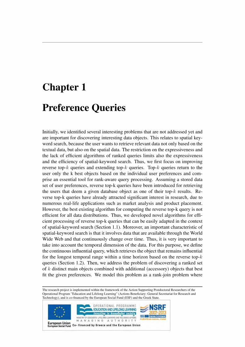
Initially, we identified several interesting problems that are not addressed yet andare important for discovering interesting data objects. This relates to spatial key-word search, because the user wants to retrieve relevant data not only based on thetextual data, but also on the spatial data. The restriction on the expressiveness andthe lack of efficient algorithms of ranked queries limits also the expressivenessand the efficiency of spatial-keyword search. Thus, we first focus on improvingreverse top-k queries and extending top-k queries. Top-k queries return to theuser only the k best objects based on the individual user preferences and com-prise an essential tool for rank-aware query processing. Assuming a stored dataset of user preferences, reverse top-k queries have been introduced for retrievingthe users that deem a given database object as one of their top-k results. Re-verse top-k queries have already attracted significant interest in research, due tonumerous real-life applications such as market analysis and product placement.However, the best existing algorithm for computing the reverse top-k query is notefficient for all data distributions. Thus, we developed novel algorithms for effi-cient processing of reverse top-k queries that can be easily adapted in the contextof spatial-keyword search (Section 1.1). Moreover, an important characteristic ofspatial-keyword search is that it involves data that are available through the WorldWide Web and that continuously change over time. Thus, it is very important totake into account the temporal dimension of the data. For this purpose, we definethe continuous influential query, which retrieves the object that remains influentialfor the longest temporal range within a time horizon based on the reverse top-kqueries (Section 1.2). Then, we address the problem of discovering a ranked setof k distinct main objects combined with additional (accessory) objects that bestfit the given preferences. We model this problem as a rank-join problem where
The research project is implemented within the framework of the Action Supporting Postdoctoral Researchers of theOperational Program ”Education and Lifelong Learning” (Actions Beneficiary: General Secretariat for Research andTechnology), and is co-financed by the European Social Fund (ESF) and the Greek State.
CHAPTER 1. PREFERENCE QUERIES
p1
p5 9.3
8.4
Huey’s top-2
id score
p2
p4
p3
p6
p5
Hotel database
id rating stars
p1 9 3
278 58 4
10 3
6 4
User preferences
user w[rating] w[stars]
Huey
Dewey0.9
Louie
0.10.80.2
0.5 0.5
p4
p3 5.6
4.8
Dewey’s top-2
id score
p5
p3 6.5
6.5
Louie’s top-2
id score
DATABASETOP-k RESULTS REVERSE TOP-k RESULTS
p1’s reverse top-2
Huey 0.9 0.1
p3’s reverse top-2
p5’s reverse top-2
Huey 0.9 0.1
p4’s reverse top-2
Dewey 0.2 0.8
Dewey 0.2 0.8
Louie 0.5 0.5
Louie 0.5 0.5
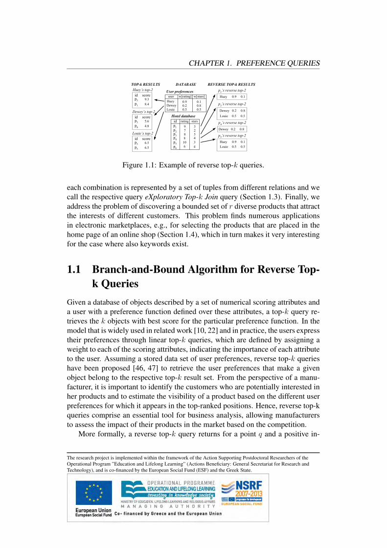
Figure 1.1: Example of reverse top-k queries.
each combination is represented by a set of tuples from different relations and wecall the respective query eXploratory Top-k Join query (Section 1.3). Finally, weaddress the problem of discovering a bounded set of r diverse products that attractthe interests of different customers. This problem finds numerous applicationsin electronic marketplaces, e.g., for selecting the products that are placed in thehome page of an online shop (Section 1.4), which in turn makes it very interestingfor the case where also keywords exist.
1.1 Branch-and-Bound Algorithm for Reverse Top-k Queries
Given a database of objects described by a set of numerical scoring attributes anda user with a preference function defined over these attributes, a top-k query re-trieves the k objects with best score for the particular preference function. In themodel that is widely used in related work [10, 22] and in practice, the users expresstheir preferences through linear top-k queries, which are defined by assigning aweight to each of the scoring attributes, indicating the importance of each attributeto the user. Assuming a stored data set of user preferences, reverse top-k querieshave been proposed [46, 47] to retrieve the user preferences that make a givenobject belong to the respective top-k result set. From the perspective of a manu-facturer, it is important to identify the customers who are potentially interested inher products and to estimate the visibility of a product based on the different userpreferences for which it appears in the top-ranked positions. Hence, reverse top-kqueries comprise an essential tool for business analysis, allowing manufacturersto assess the impact of their products in the market based on the competition.
More formally, a reverse top-k query returns for a point q and a positive in-
The research project is implemented within the framework of the Action Supporting Postdoctoral Researchers of theOperational Program ”Education and Lifelong Learning” (Actions Beneficiary: General Secretariat for Research andTechnology), and is co-financed by the European Social Fund (ESF) and the Greek State.

CHAPTER 1. PREFERENCE QUERIES
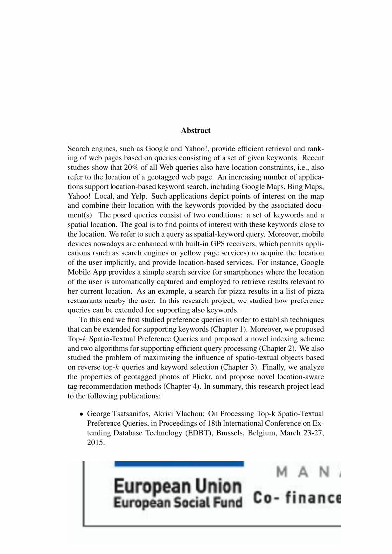
teger k, the set of linear preference functions (in terms of weighting vectors) forwhich q is contained in their top-k result. Consider for example a database con-taining information about different hotels as well as user preferences, as depictedin Figure 2.1. For each of the six hotels, the rating and the number of stars arerecorded, and maximum values on each attribute are preferable. The database alsostores the preferences of three users (Huey, Dewey and Louie) in terms of weightson each attribute. Different users may have different preferences about a potentialhotel. For instance, Huey prefers hotels with high rating values, whereas Deweyis interested in hotels with many stars. Louie is indifferent or values equally ratingand stars. On the left part of the figure, the top-2 hotels are depicted for each useralong with their scores. On the right part, the reverse top-2 results are shown forthe hotels. Notice that p2 and p6 have empty reverse top-2 result sets, i.e., they donot belong to the top-2 list of any user.
Currently, the most efficient algorithm for computing the reverse top-k setis the RTA algorithm [46]. RTA has two main drawbacks when processing areverse top-k query: (i) it needs to access all stored user preferences, and (ii)it cannot avoid executing a top-k query for each user preference (determined bythe corresponding user weights) that belongs to the result set. As a result, theperformance of RTA is sensitive to the cardinality of the reverse top-k result; forqueries with result sets of high cardinality RTA often becomes inefficient. Sincewe expect that reverse top-k queries will be posed for query points that are highlyranked, and therefore have a result set of high cardinality, this drawback severelylimits the practicality of RTA.
To alleviate the shortcomings of RTA, we study the conditions in which a setof weighting vectors (representing linear preference functions) can be immedi-ately added to the result set. Therefore, we focus on whether a data point maybe ranked higher than the query point for a set of weighting vectors. In addi-tion, we address the question whether a set of weighting vectors can be excludedfrom the reverse top-k result. Based on these properties, we develop an efficientbranch-and-bound algorithm assuming that both data sets are indexed by multidi-mensional access methods.
The contributions of this work are summarized here:
• We introduce useful properties for processing reverse top-k queries withoutaccessing each user’s individual preferences nor executing the respectivetop-k query.
• We present a novel algorithm that processes sets of weighting vectors, with-out having to examine each vector individually, and use this algorithm as
The research project is implemented within the framework of the Action Supporting Postdoctoral Researchers of theOperational Program ”Education and Lifelong Learning” (Actions Beneficiary: General Secretariat for Research andTechnology), and is co-financed by the European Social Fund (ESF) and the Greek State.
CHAPTER 1. PREFERENCE QUERIES
basic building block for our reverse top-k algorithms.
• We propose a framework for reverse top-k query processing that employsthe branch-and-bound methodology and exploits the introduced properties.
• We present two optimizations of the basic branch-and-bound algorithm (BBR)that use result sharing (BBR∗) and an aggregate R-tree (BBRA) to boostits performance.
• We conduct a thorough experimental evaluation that demonstrates the effi-ciency of our proposed algorithms.
For more details refer to: Akrivi Vlachou, Christos Doulkeridis, Kjetil Nørvagand Yannis Kotidis: Branch-and-Bound Algorithm for Reverse Top-k Queries,in Proceedings of ACM International Conference on Management of Data (SIG-MOD), New York, USA, June 22-27, 2013.
1.2 Discovering Influential Data Objects over TimeIn online marketplaces, top-k queries are typically used to present a limited num-ber of products ranked according to the user’s preferences. This is extremelyhelpful for the user as it enables decision-making, without the need to inspectlarge amounts of possibly uninteresting results. In addition, the user is not over-whelmed by the available information and can retrieve results that satisfy her in-formation need. As a result, an increasing amount of research has focused onefficient techniques for top-k query processing lately [24].
From the perspective of the product manufacturers top-k queries are of greatinterest as well, since the visibility of a product clearly depends on the number ofdifferent top-k queries for which it belongs to the result set. The reason for this istwofold: 1) users usually consider only a few highly ranked products and ignorethe remaining ones, and 2) products that appear in the top-k result sets are farmore likely to be chosen by a potential customer, because these products satisfythe customers’ preferences. Recently, reverse top-k queries [46] were proposed tostudy the visibility of a given product. A reverse top-k query returns the set of userpreferences (i.e., customers) for which a given product is in the result set of therespective top-k queries. Intuitively, a product that appears in as many as possibletop-k result sets, has a higher visibility and therefore also a higher impact on themarket. This has naturally lead to the definition of the most influential products
The research project is implemented within the framework of the Action Supporting Postdoctoral Researchers of theOperational Program ”Education and Lifelong Learning” (Actions Beneficiary: General Secretariat for Research andTechnology), and is co-financed by the European Social Fund (ESF) and the Greek State.
CHAPTER 1. PREFERENCE QUERIES
based on the cardinality of their reverse top-k result sets [48]. Identifying the mostinfluential products from a given set of products is important for market analysis,since the product manufacturer can estimate the impact of her products in themarket.
However, an important aspect of a product’s influence that has not been takeninto account yet is its variance over time as the user preferences change. Thecustomers’ criteria can differ significantly over time for various reasons. For ex-ample, in online marketplaces, new customers pose queries and new preferencesare collected. In addition, customers that have already posed queries will dis-connect after some time. As user preferences change over time, a product whichappears consistently in the top-k results of as many customers as possible, thussatisfying many customers’ criteria at any time, has a higher impact on the marketthan a product that is absent from those results. Therefore, these products are thebest candidate products to advertise to potential customers, and it is important toidentify such products efficiently.
In this work, we study for the first time the problem of finding the product thatbelongs consistently to the most influential products over time, the continuous in-fluential products. This is an important problem for many real-life applications.For example, the products advertised on the first page of an online marketplaceshould be the products that have the greatest impact on the market, i.e., the prod-ucts that are the most popular among the customers. Since customers change allthe time, the products that consistently belong to the most influential productsover time are more probable to attract many potential customers at any time. Itis therefore essential to identify the objects (products) that have high impact overa period of time and despite the fluctuation of preferences these objects remainamong the most influential objects. From now on we will use the terms productand object interchangeably.
In the following, we first define formally the problem of continuous influentialproducts and provide a baseline algorithm that sequentially scans all time intervalsin order to retrieve the most continuous influential product. Then, we provide abounding scheme in order to facilitate early termination of our algorithms andavoid processing time intervals that do not alter the result set. Summarizing, themain contributions of this work are:
• We study, for the first time, the problem of identifying the data object thathas the highest impact over time.
• An appropriate score of influence (called continuity score) based on thereverse top-k query is defined to capture the product impact over a period
The research project is implemented within the framework of the Action Supporting Postdoctoral Researchers of theOperational Program ”Education and Lifelong Learning” (Actions Beneficiary: General Secretariat for Research andTechnology), and is co-financed by the European Social Fund (ESF) and the Greek State.
CHAPTER 1. PREFERENCE QUERIES
of time.
• We derive upper and lower bounds for the continuity score of a given objectthat lead to efficient algorithms for retrieving the most continuous influ-ential product. Two different algorithms are presented that provide earlytermination based on the bounds, but follow different strategies in order toterminate as soon as possible.
• We conduct a detailed experimental study for various setups and demon-strate the efficiency of our algorithms.
For more details refer to: Orestis Gkorgkas, Akrivi Vlachou, Christos Doulk-eridis and Kjetil Nørvag: Discovering Influential Data Objects over Time, in Pro-ceedings of 13th International Symposium on Spatial and Temporal Databases(SSTD), Munich, Germany, August 21-23, 2013.
1.3 Efficient Processing of Exploratory Top-k JoinsTop-k queries [24] are often used to help users select the k best objects accordingto their preferences from a large set of objects. A product is typically representedby a d-dimensional point p where each dimension describes a specific feature.Usually, preferences are expressed through a weighting vector w of d dimensions,each corresponding to an attribute of the product, while the value of the dimensionindicates the importance of the specific attribute to the user. The ranking of theobjects is based on a scoring function fw(p), and one of the most common ones isthe weighted sum fw(p) =
∑di w[i]p[i].
To this end, we propose the eXploratory Top-k Join (XTJk) query. An XTJktakes as input a a set of relations where there is a main relation and the rest ad-ditional relations are joined to the main relation forming a ”star”-like structure.Among all possible combinations, only the best for each product are consideredand the top-k of them are returned to the user.
Current state-of-the-art techniques [18, 23, 40] for computing combinationsbased on preference vectors fall short to address this kind of queries as they as-sume that each result should contain objects from all relations participating in thejoin. On the contrary, our requirement is that an object should be added to a com-bination only if it is beneficial for the combination. Moreover, current techniquesdo not exploit the form of the result-set and the structure of the join, fact that leadsto suboptimal performance.
The research project is implemented within the framework of the Action Supporting Postdoctoral Researchers of theOperational Program ”Education and Lifelong Learning” (Actions Beneficiary: General Secretariat for Research andTechnology), and is co-financed by the European Social Fund (ESF) and the Greek State.
CHAPTER 1. PREFERENCE QUERIES
To summarize, the contributions of this work are: a) we introduce the eX-ploratory Top-k Join (XTJk) query, a novel query type which creates combinationsof variable size between main and additional objects and returns the top-k combi-nations with discrete main objects, b) we introduce an efficient bounding schemefor our algorithm, and c) we perform an experimental evaluation that demonstratesthe efficiency of our approach.
For more details refer to: Orestis Gkorgkas, Akrivi Vlachou, Christos Doulk-eridis and Kjetil Nørvag: Efficient Processing of Exploratory Top-k Joins, in Pro-ceedings of 26th International Conference on Scientific and Statistical DatabaseManagement (SSDBM), Aalborg, Denmark, June 30 - July 2, 2014.
1.4 Finding the Most Diverse Products using Pref-erence Queries
Top-k queries [44] help customers select a ranked set of k products that best matchtheir preferences out of an overwhelmingly large collection of products. For aspecific customer, her preferences are expressed by means of a top-k query, andhighly ranked products in the top-k result are more attractive to the customer.Thus, from the perspective of product sellers, the visibility and the potential mar-ket of a product relates to the top-k queries for which the product is highly ranked.Towards this direction, reverse top-k queries [46] retrieve the set of user prefer-ences for which a product appears in their top-k lists. Reverse top-k queries arevery important for estimating the impact of the product on the market, as the car-dinality of the result set defines an influence score [49] for the product, i.e., thenumber of customers that value a particular product.
We study the problem of finding the r most diverse products based on theuser preferences. The goal is to find a set of products that are attractive to awide range of customers with different preferences. For instance, consider anelectronic marketplace that wishes to advertise r products on its front page aimingto attract as many new customers as possible. Advertising diverse products thatare attractive to different existing customers increases the probability that a newcustomer finds one of those products attractive. The strategy of advertising ther most influential products [49], i.e., the r products that attract the highest totalnumber of customers, does not necessarily lead to a set of diverse products andmay fail to attract many new customers, since such products may be attractive tocustomers with similar preferences.
The research project is implemented within the framework of the Action Supporting Postdoctoral Researchers of theOperational Program ”Education and Lifelong Learning” (Actions Beneficiary: General Secretariat for Research andTechnology), and is co-financed by the European Social Fund (ESF) and the Greek State.
CHAPTER 1. PREFERENCE QUERIES
User Preferences:
User w[1] w[2] w[3] Top-kBob 0.1 0.2 0.7 p1
Tom 0.1 0.3 0.6 p1
Jack 0.3 0.1 0.6 p2
Max 0.8 0.1 0.1 p3
Products:
Product p[1] p[2] p[3] Reverse top-kp1 1 2 6 Bob,Tomp2 2 1 6 Jackp3 6 5 2 Max
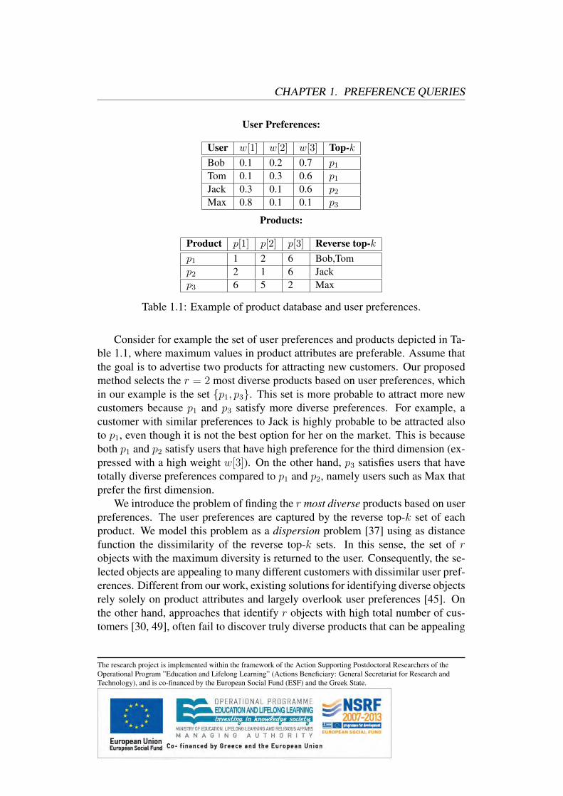
Table 1.1: Example of product database and user preferences.
Consider for example the set of user preferences and products depicted in Ta-ble 1.1, where maximum values in product attributes are preferable. Assume thatthe goal is to advertise two products for attracting new customers. Our proposedmethod selects the r = 2 most diverse products based on user preferences, whichin our example is the set {p1, p3}. This set is more probable to attract more newcustomers because p1 and p3 satisfy more diverse preferences. For example, acustomer with similar preferences to Jack is highly probable to be attracted alsoto p1, even though it is not the best option for her on the market. This is becauseboth p1 and p2 satisfy users that have high preference for the third dimension (ex-pressed with a high weight w[3]). On the other hand, p3 satisfies users that havetotally diverse preferences compared to p1 and p2, namely users such as Max thatprefer the first dimension.
We introduce the problem of finding the r most diverse products based on userpreferences. The user preferences are captured by the reverse top-k set of eachproduct. We model this problem as a dispersion problem [37] using as distancefunction the dissimilarity of the reverse top-k sets. In this sense, the set of robjects with the maximum diversity is returned to the user. Consequently, the se-lected objects are appealing to many different customers with dissimilar user pref-erences. Different from our work, existing solutions for identifying diverse objectsrely solely on product attributes and largely overlook user preferences [45]. Onthe other hand, approaches that identify r objects with high total number of cus-tomers [30, 49], often fail to discover truly diverse products that can be appealing
The research project is implemented within the framework of the Action Supporting Postdoctoral Researchers of theOperational Program ”Education and Lifelong Learning” (Actions Beneficiary: General Secretariat for Research andTechnology), and is co-financed by the European Social Fund (ESF) and the Greek State.

CHAPTER 1. PREFERENCE QUERIES
to new customers with different preferences than those of the existing ones.To summarize the contributions of this work are:
• We study the novel problem of finding the r most diverse products based onuser preferences. We model this problem as a dispersion problem and definean appropriate distance function that captures the dissimilarity of productsbased on their reverse top-k sets.
• As dispersion problems are known to be NP-hard [16], we use a greedyalgorithm that retrieves r diverse products, after computing the reverse top-k sets of the products efficiently.
• To improve the performance of our algorithm, we propose an alternativealgorithm that progressively computes an approximation of the reverse top-k sets of a limited set of candidate products and retrieves a set of r productsof high diversity.
• We present maintenance techniques for updating the r most diverse prod-ucts in the case of dynamic data in a cost-efficient way. In addition, wegeneralize our approach to support any set-based similarity function.
• We demonstrate the efficiency and achieved diversity of our algorithms us-ing both synthetic and real-life data sets.
For more details refer to: Orestis Gkorgkas, Akrivi Vlachou, Christos Doulk-eridis and Kjetil Nørvag: Finding the Most Diverse Products using PreferenceQueries, in Proceedings of 18th International Conference on Extending DatabaseTechnology (EDBT), Brussels, Belgium, March 23-27, 2015.
The research project is implemented within the framework of the Action Supporting Postdoctoral Researchers of theOperational Program ”Education and Lifelong Learning” (Actions Beneficiary: General Secretariat for Research andTechnology), and is co-financed by the European Social Fund (ESF) and the Greek State.
Chapter 2
On Processing Top-k Spatio-TextualPreference Queries
In this work we propose a novel query type, termed top-k spatio-textual prefer-ence query, that retrieves a set of spatio-textual objects ranked by the goodnessof the facilities in their neighborhood. Consider for example, a tourist that looksfor “hotels that have nearby a highly rated Italian restaurant that serves pizza”.The proposed query type takes into account not only the spatial location andtextual description of spatio-textual objects (such as hotels and restaurants), butalso additional information such as ratings that describe their quality. Moreover,spatio-textual objects (i.e., hotels) are ranked based on the features of facilities(i.e., restaurants) in their neighborhood. Computing the score of each data objectbased on the facilities in its neighborhood is costly. To address this limitation,we propose an appropriate indexing technique and develop an efficient algorithmfor processing our novel query. Moreover, we extend our algorithm for process-ing spatio-textual preference queries based on alternative score definitions undera unified framework. Last but not least, we conduct extensive experiments forevaluating the performance of our methods.
2.1 IntroductionAn increasing number of applications support location-based queries, which re-trieve the most interesting spatial objects based on their geographic location. Re-cently, spatio-textual queries have lavished much attention, as such queries com-bine location-based retrieval with textual information that describes the spatial
The research project is implemented within the framework of the Action Supporting Postdoctoral Researchers of theOperational Program ”Education and Lifelong Learning” (Actions Beneficiary: General Secretariat for Research andTechnology), and is co-financed by the European Social Fund (ESF) and the Greek State.

CHAPTER 2. ON PROCESSING TOP-K SPATIO-TEXTUAL PREFERENCEQUERIES
objects. Most of the existing queries only focus on retrieving objects that satisfy aspatial constraint ranked by their spatio-textual similarity to the query point. How-ever, in addition users are quite often interested in spatial objects (data objects)based on the quality of other facilities (feature objects) that are located in theirvicinity. Feature objects are typically described by non-spatial attributes suchas quality or rating, in addition to the textual description. We propose a noveland more expressive query type than existing spatio-textual queries, called top-kspatio-textual preference query, for ranked retrieval of data objects based the tex-tual relevance and the non-spatial score of feature objects in their neighborhood.
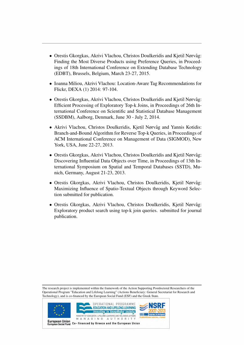
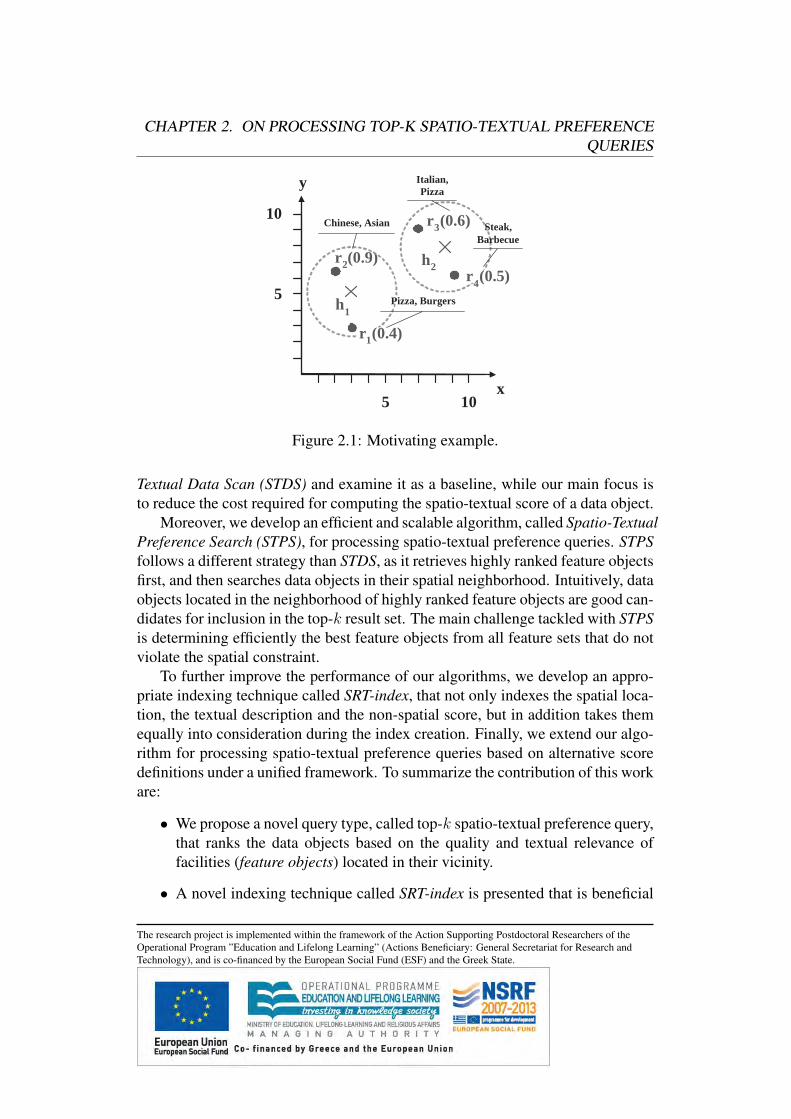
Consider for example, a tourist that looks for “hotels that have nearby a highlyrated Italian restaurant that serves pizza”. Figure 2.1 depicts a spatial area con-taining hotels (data objects) and restaurants (feature objects). The quality of therestaurants based on existing reviews is depicted next to the restaurant. Eachrestaurant also has textual information in the form of keywords extracted fromits menu, such as pizza or steak, which describes additional characteristics of therestaurant. The tourist also specifies a spatial constraint (in the figure depicted asa range around each hotel) to restrict the distance of the restaurant to the hotel.Obviously, the hotel h2 is the best option for a tourist that poses the aforemen-tioned query. In the general case, more than one type of feature objects may existin order to support queries such as “hotels that have nearby a good Italian restau-rant that serves pizza and a cheap coffeehouse that serves muffins”. Even thoughspatial preference queries have been studied before [53, 54, 39], their definitionignores the available textual information. In our example, the spatial preferencequery would correspond to a tourist that searches for “hotels that are nearby agood restaurant” and the hotel h1 would always be retrieved, irrespective of thetextual information.
We define top-k spatio-textual preference queries and provide efficient algo-rithms for processing this novel query type. A main challenge compared to tra-ditional spatial preference queries [53, 54, 39] is that the score of a data objectchanges depending on the query keywords, which renders techniques that rely onmaterialization (such as [39]) not applicable. Most importantly, processing spa-tial preference queries is costly in terms of both I/O and execution time [53, 54].Thus, extending spatial preference queries for supporting also textual informationis challenging, since the new query type is more demanding due to the additionaltextual descriptions.
A straightforward algorithm for processing spatio-textual preference queriesis to compute the spatio-textual preference score for each data object and thenreport the k data objects with the highest score. We call this approach Spatio-
The research project is implemented within the framework of the Action Supporting Postdoctoral Researchers of theOperational Program ”Education and Lifelong Learning” (Actions Beneficiary: General Secretariat for Research andTechnology), and is co-financed by the European Social Fund (ESF) and the Greek State.
CHAPTER 2. ON PROCESSING TOP-K SPATIO-TEXTUAL PREFERENCEQUERIES
r 2 (0.9)
5
10
5 10 x
y
h 1
h 2
r 3 (0.6)
r 1 (0.4)
Chinese, Asian
Italian, Pizza
Steak, Barbecue
Pizza, Burgers
r 4 (0.5)
Figure 2.1: Motivating example.
Textual Data Scan (STDS) and examine it as a baseline, while our main focus isto reduce the cost required for computing the spatio-textual score of a data object.
Moreover, we develop an efficient and scalable algorithm, called Spatio-TextualPreference Search (STPS), for processing spatio-textual preference queries. STPSfollows a different strategy than STDS, as it retrieves highly ranked feature objectsfirst, and then searches data objects in their spatial neighborhood. Intuitively, dataobjects located in the neighborhood of highly ranked feature objects are good can-didates for inclusion in the top-k result set. The main challenge tackled with STPSis determining efficiently the best feature objects from all feature sets that do notviolate the spatial constraint.
To further improve the performance of our algorithms, we develop an appro-priate indexing technique called SRT-index, that not only indexes the spatial loca-tion, the textual description and the non-spatial score, but in addition takes themequally into consideration during the index creation. Finally, we extend our algo-rithm for processing spatio-textual preference queries based on alternative scoredefinitions under a unified framework. To summarize the contribution of this workare:
• We propose a novel query type, called top-k spatio-textual preference query,that ranks the data objects based on the quality and textual relevance offacilities (feature objects) located in their vicinity.
• A novel indexing technique called SRT-index is presented that is beneficial
The research project is implemented within the framework of the Action Supporting Postdoctoral Researchers of theOperational Program ”Education and Lifelong Learning” (Actions Beneficiary: General Secretariat for Research andTechnology), and is co-financed by the European Social Fund (ESF) and the Greek State.
CHAPTER 2. ON PROCESSING TOP-K SPATIO-TEXTUAL PREFERENCEQUERIES
for processing spatio-textual preference queries.
• We present two algorithms for processing spatio-textual preference queries,namely Spatio-Textual Data Scan (STDS) and Spatio-Textual PreferenceSearch (STPS).
• We extend our algorithm STPS for processing spatio-textual preference queriesbased on alternative score definitions under a unified framework.
• We conduct an extensive experiment evaluation for studying the perfor-mance of our proposed algorithms and indexing technique.
The rest of this chapter is organized as follows: Section 4.5 overviews the rel-evant literature. In Section 2.3, we define the spatio-textual preference query. Ournovel indexing technique (SRT-index) is presented in Section 2.4. In Section 2.5we describe our baseline algorithm, called spatio-textual data scan (STDS). Anefficient algorithm, called Spatio-Textual Preference Search (STPS), is proposedin Section 2.6. Moreover, we extend our algorithms for processing spatio-textualpreference queries based on alternative scores in Section 2.7. We present the ex-perimental evaluation in Section 2.8 and we conclude in Section 3.8.
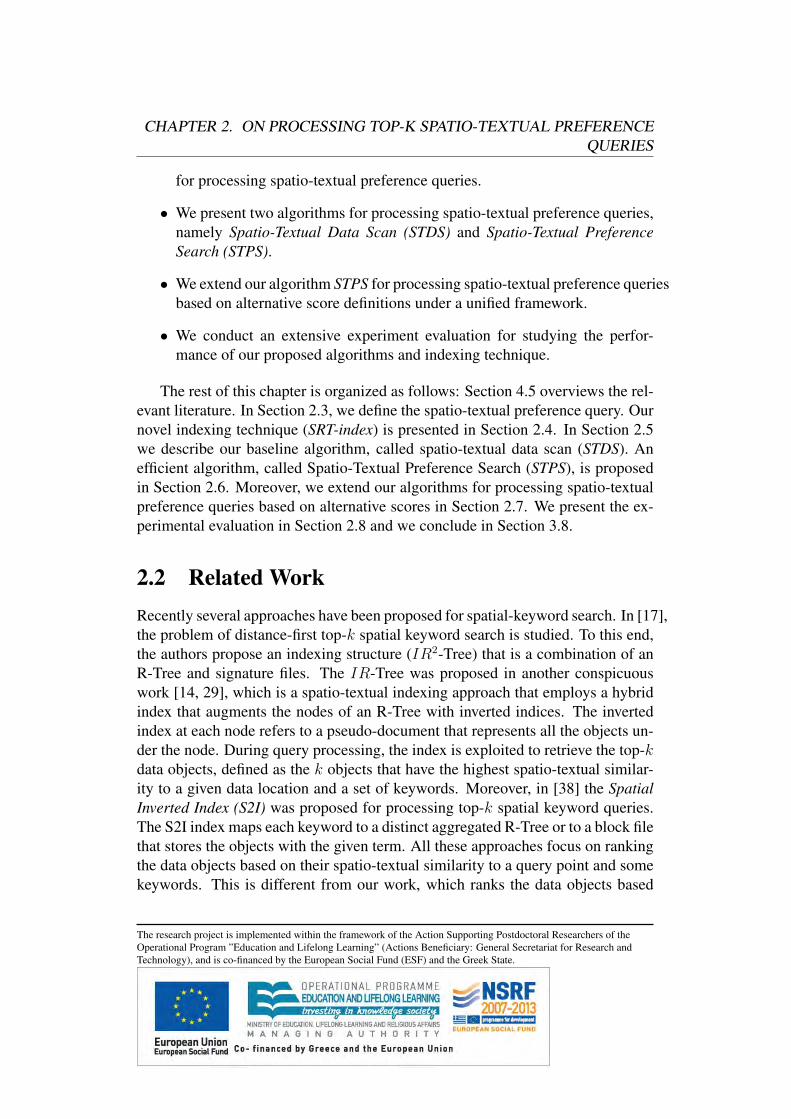
2.2 Related WorkRecently several approaches have been proposed for spatial-keyword search. In [17],the problem of distance-first top-k spatial keyword search is studied. To this end,the authors propose an indexing structure (IR2-Tree) that is a combination of anR-Tree and signature files. The IR-Tree was proposed in another conspicuouswork [14, 29], which is a spatio-textual indexing approach that employs a hybridindex that augments the nodes of an R-Tree with inverted indices. The invertedindex at each node refers to a pseudo-document that represents all the objects un-der the node. During query processing, the index is exploited to retrieve the top-kdata objects, defined as the k objects that have the highest spatio-textual similar-ity to a given data location and a set of keywords. Moreover, in [38] the SpatialInverted Index (S2I) was proposed for processing top-k spatial keyword queries.The S2I index maps each keyword to a distinct aggregated R-Tree or to a block filethat stores the objects with the given term. All these approaches focus on rankingthe data objects based on their spatio-textual similarity to a query point and somekeywords. This is different from our work, which ranks the data objects based
The research project is implemented within the framework of the Action Supporting Postdoctoral Researchers of theOperational Program ”Education and Lifelong Learning” (Actions Beneficiary: General Secretariat for Research andTechnology), and is co-financed by the European Social Fund (ESF) and the Greek State.
CHAPTER 2. ON PROCESSING TOP-K SPATIO-TEXTUAL PREFERENCEQUERIES
on textual relevance and a non-spatial score (quality) of the facilities in their spa-tial neighborhood. [11] provides an all-around evaluation of spatio-textual indicesand reports on the findings obtained when applying a benchmark to the indices.
Spatio-textual similarity joins were studied in [4]. Given two data sets, thequery retrieves all pairs of objects that have spatial distance smaller than a givenvalue and at the same time a textual similarity that is larger than a given value.This differs from the top-k spatio-textual preferences query, because the spatio-textual similarity join does not rank the data objects and some data objects mayappear more than once in the result set. Prestige-based spatio-textual retrieval wasstudied in [7]. The proposed query takes into account both location proximity andprestige-based text relevance.
The m-closest keywords query [55] aims to find the spatially closest data ob-jects that match with the query keywords. The authors in [8] study the spatialgroup keyword query that retrieves a group of data objects such that all querykeywords appear in at least one data object textual description and such that ob-jects are nearest to the query location and have the lowest inter-object distances.These approaches focus on finding a set of data objects that are close to eachother and relevant to a given query, whereas in this work we rank the data objectsbased on the facilities in their spatial neighborhood. In [9], the length-constrainedmaximum-sum region (LCMSR) query is proposed that returns a spatial-networkregion of constrained size that is located within a general region of interest andthat best matches query keywords.
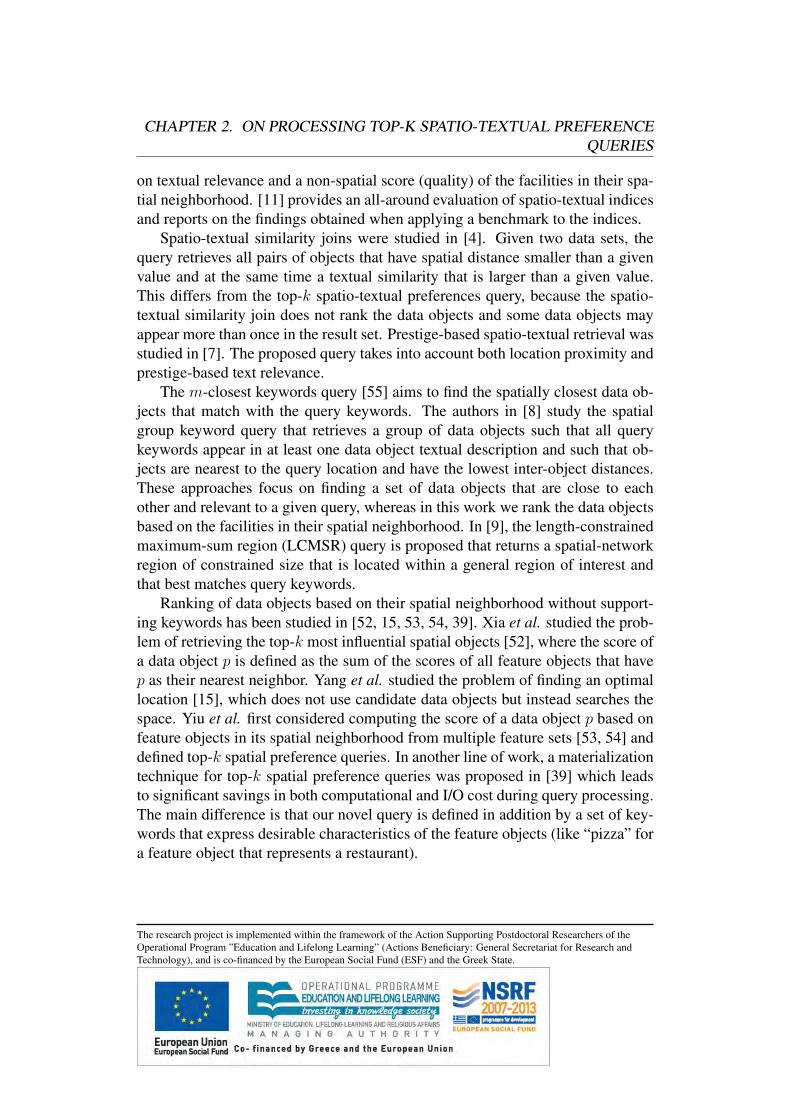
Ranking of data objects based on their spatial neighborhood without support-ing keywords has been studied in [52, 15, 53, 54, 39]. Xia et al. studied the prob-lem of retrieving the top-k most influential spatial objects [52], where the score ofa data object p is defined as the sum of the scores of all feature objects that havep as their nearest neighbor. Yang et al. studied the problem of finding an optimallocation [15], which does not use candidate data objects but instead searches thespace. Yiu et al. first considered computing the score of a data object p based onfeature objects in its spatial neighborhood from multiple feature sets [53, 54] anddefined top-k spatial preference queries. In another line of work, a materializationtechnique for top-k spatial preference queries was proposed in [39] which leadsto significant savings in both computational and I/O cost during query processing.The main difference is that our novel query is defined in addition by a set of key-words that express desirable characteristics of the feature objects (like “pizza” fora feature object that represents a restaurant).
The research project is implemented within the framework of the Action Supporting Postdoctoral Researchers of theOperational Program ”Education and Lifelong Learning” (Actions Beneficiary: General Secretariat for Research andTechnology), and is co-financed by the European Social Fund (ESF) and the Greek State.
CHAPTER 2. ON PROCESSING TOP-K SPATIO-TEXTUAL PREFERENCEQUERIES
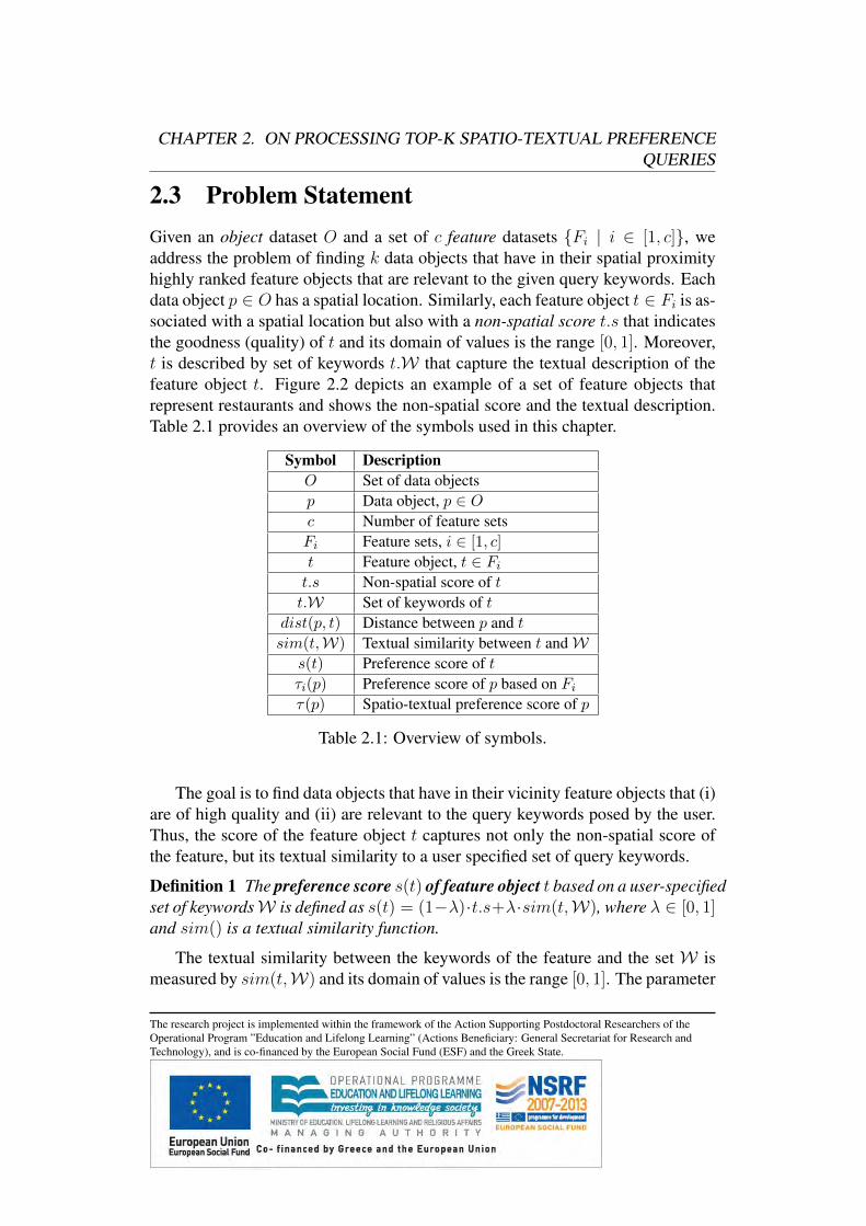
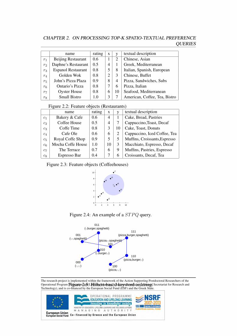
2.3 Problem StatementGiven an object dataset O and a set of c feature datasets {Fi | i ∈ [1, c]}, weaddress the problem of finding k data objects that have in their spatial proximityhighly ranked feature objects that are relevant to the given query keywords. Eachdata object p ∈ O has a spatial location. Similarly, each feature object t ∈ Fi is as-sociated with a spatial location but also with a non-spatial score t.s that indicatesthe goodness (quality) of t and its domain of values is the range [0, 1]. Moreover,t is described by set of keywords t.W that capture the textual description of thefeature object t. Figure 2.2 depicts an example of a set of feature objects thatrepresent restaurants and shows the non-spatial score and the textual description.Table 2.1 provides an overview of the symbols used in this chapter.
Symbol DescriptionO Set of data objectsp Data object, p ∈ Oc Number of feature setsFi Feature sets, i ∈ [1, c]
t Feature object, t ∈ Fi
t.s Non-spatial score of tt.W Set of keywords of t
dist(p, t) Distance between p and tsim(t,W) Textual similarity between t andW
s(t) Preference score of tτi(p) Preference score of p based on Fi
τ(p) Spatio-textual preference score of p
Table 2.1: Overview of symbols.
The goal is to find data objects that have in their vicinity feature objects that (i)are of high quality and (ii) are relevant to the query keywords posed by the user.Thus, the score of the feature object t captures not only the non-spatial score ofthe feature, but its textual similarity to a user specified set of query keywords.
Definition 1 The preference score s(t) of feature object t based on a user-specifiedset of keywordsW is defined as s(t) = (1−λ)·t.s+λ·sim(t,W), where λ ∈ [0, 1]and sim() is a textual similarity function.
The textual similarity between the keywords of the feature and the set W ismeasured by sim(t,W) and its domain of values is the range [0, 1]. The parameter
The research project is implemented within the framework of the Action Supporting Postdoctoral Researchers of theOperational Program ”Education and Lifelong Learning” (Actions Beneficiary: General Secretariat for Research andTechnology), and is co-financed by the European Social Fund (ESF) and the Greek State.

CHAPTER 2. ON PROCESSING TOP-K SPATIO-TEXTUAL PREFERENCEQUERIES
λ is the smoothing parameter that determines how much the score of the featureobjects should be influenced by the textual information. For the rest of the chapter,we assume that the textual similarity is equal to the Jaccard similarity between thekeywords of the feature objects and the user-specified keywords: sim(t,W) =|t.W
⋂W|
|t.W⋃W| .
For example, consider the restaurants depicted in Figure 2.2. Given a set ofkeywords W = {italian, pizza} and λ = 0.5 the restaurant with the highestpreference score is Ontario’s Pizza with a preference score s(r6) = 0.9, while thescore of Beijing Restaurant is s(r1) = 0.3, since none of the given keywords areincluded in the description of Beijing Restaurant.
Given a spatio-textual preference query Q defined by an integer k, a range rand c-sets of keywords Wi, the preference score of a data object p ∈ O basedon a feature set Fi is defined by the scores of feature objects t ∈ Fi in its spatialneighborhood, whereas the overall spatio-textual score of p is defined by takinginto account all feature sets Fi, 1 ≤ i ≤ c.
Definition 2 The preference score τi(p) of data object p based on the feature setFi is defined as: τi(p) = max{s(t) | t ∈ Fi : dist(p, t) ≤ r and sim(t,Wi) >0}.
The dist(p, t) denotes the spatial distance between data object p and featureobject t and we employ the Euclidean distance function. Continuing the previousexample, Figure 2.4 shows the spatial location of the restaurants in Figure 2.2and a data point p that represents a hotel. The preference score of p based on therestaurants in its neighborhood (assuming r = 3.5 andW = {italian, pizza}) isequal to the score of r6 (τi(p) = s(r6) = 0.9), which is the best restaurant in theneighborhood of p.
Definition 3 The overall spatio-textual preference score τ(p) of data object p isdefined as: τ(p) =
∑i∈[1,c] τi(p).
Figure 2.3 shows a second set of feature objects that represents coffeehouses.For a tourist that looks for a good hotel that has nearby a good Italian restaurantthat serves pizza and a good coffeehouse that serves espresso and muffins, thescore of p would be τ(p) = s(r6) + s(c5) = 0.9 + 0.78233 = 1.6833.
Problem 1 Top-k Spatio-Textual Preference Queries (STPQ): Given a query Q,defined by an integer k, a radius r and c-sets of keywords Wi, find the k dataobjects p ∈ O with the highest spatio-textual score τ(p).
The research project is implemented within the framework of the Action Supporting Postdoctoral Researchers of theOperational Program ”Education and Lifelong Learning” (Actions Beneficiary: General Secretariat for Research andTechnology), and is co-financed by the European Social Fund (ESF) and the Greek State.
CHAPTER 2. ON PROCESSING TOP-K SPATIO-TEXTUAL PREFERENCEQUERIES
name rating x y textual descriptionr1 Beijing Restaurant 0.6 1 2 Chinese, Asianr2 Daphne’s Restaurant 0.5 4 1 Greek, Mediterraneanr3 Espanol Restaurant 0.8 5 8 Italian, Spanish, Europeanr4 Golden Wok 0.8 2 3 Chinese, Buffetr5 John’s Pizza Plaza 0.9 8 4 Pizza, Sandwiches, Subsr6 Ontario’s Pizza 0.8 7 6 Pizza, Italianr7 Oyster House 0.8 6 10 Seafood, Mediterraneanr8 Small Bistro 1.0 3 7 American, Coffee, Tea, Bistro
Figure 2.2: Feature objects (Restaurants)name rating x y textual description
c1 Bakery & Cafe 0.6 4 1 Cake, Bread, Pastriesc2 Coffee House 0.5 4 7 Cappuccino,Toast, Decafc3 Coffe Time 0.8 3 10 Cake, Toast, Donutsc4 Cafe Ole 0.6 6 2 Cappuccino, Iced Coffee, Teac5 Royal Coffe Shop 0.9 5 5 Muffins, Croissants,Espressoc6 Mocha Coffe House 1.0 10 3 Macchiato, Espresso, Decafc7 The Terrace 0.7 6 9 Muffins, Pastries, Espressoc8 Espresso Bar 0.4 7 6 Croissants, Decaf, Tea
Figure 2.3: Feature objects (Coffeehouses)
0
2
4
6
8
10
0 2 4 6 8 10
p
r1
r2
r3
r4
r5
r6
r7
r8
Figure 2.4: An example of a STPQ query.
000
010
011
001
(pizza,-,spaghetti)
111
110
100(-,-,-)
(-,burger,-)
(-,burger,spaghetti)
(-,-,spaghetti)
101
(pizza,burger,spaghetti)
(pizza,burger,-)
(pizza,-,-)
Figure 2.5: Hilbert-based keyword ordering.The research project is implemented within the framework of the Action Supporting Postdoctoral Researchers of theOperational Program ”Education and Lifelong Learning” (Actions Beneficiary: General Secretariat for Research andTechnology), and is co-financed by the European Social Fund (ESF) and the Greek State.
CHAPTER 2. ON PROCESSING TOP-K SPATIO-TEXTUAL PREFERENCEQUERIES
2.4 IndexingThe main difference of top-k spatio-textual preference queries to traditional spatio-textual search is that the ranking of a data object does not depend only on spatiallocation and textual information, but also on the non-spatial score of the featureobject. In particular, the preference score s(t) of feature object t is defined by itstextual description and its non-spatial score, while the spatial location is used asa filter for computing the preference score τi(p) of data object p. Thus, efficientindexing of the textual description and the non-spatial score of feature objects is asignificant factor for designing efficient algorithms for the STPQ query.
2.4.1 Index CharacteristicsWe assume that the data objects O are indexed by an R-Tree, denoted as rtree.However, for the feature objects, it is important that the non-spatial score andthe textual description are indexed additionally. Each dataset Fi can be indexedby any spatio-textual index that relies on a spatial hierarchical index (such as theR-Tree). However, each entry e of the index must in addition maintain: (i) themaximum value of t.s of any feature object t in the sub-tree, denoted as e.s, and(ii) a summary (e.W) of all keywords of any feature t in the sub-tree. To ensurecorrectness of our algorithms, there must exist an upper bound s(e) such that forany t stored in the sub-tree rooted by the entry e it holds:
s(e) ≥ s(t)
The above property guarantees that the preference score s(t) of a feature objectt is bounded by the bound s(e) of its ancestor node e. The efficiency of thealgorithms directly depends on the tightness of this bound. In turn, this dependson the similarity between the textual description and the non-spatial score of thefeatures objects that are indexed in the same node.
In the following, we propose an indexing technique that leads to tight boundssince objects with similar textual information and non-spatial score are stored inthe same node of the index.
2.4.2 Indexing based on Hilbert MappingOur indexing approach maps the textual description of feature objects to a valuebased on the Hilbert curve. Let w denote the number of distinct keywords in the
The research project is implemented within the framework of the Action Supporting Postdoctoral Researchers of theOperational Program ”Education and Lifelong Learning” (Actions Beneficiary: General Secretariat for Research andTechnology), and is co-financed by the European Social Fund (ESF) and the Greek State.
CHAPTER 2. ON PROCESSING TOP-K SPATIO-TEXTUAL PREFERENCEQUERIES
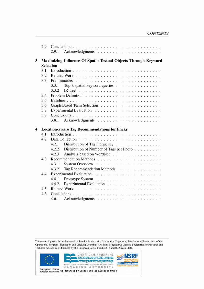
vocabulary, then for each feature t the keywords t.W can be represented as a bi-nary vector of lengthw. For instance, assuming a vocabulary {pizza, burger, spaghetti},we can use an active bit to declare the existence of the “pizza” keyword at the firstplace, “burger” at the second, and “spaghetti” at the last. Moreover, we suggesta mapping of the binary vector to a Hilbert value, denoted as H(t.W). For theabove w=3 keywords, the defined order is 000,010,011,001,101,111,110 and 100.Figure 2.5 shows the ordering of the keywords based on the Hilbert values. Thebenefit of this order is that it ensures us that vectors with distance 1 have onlyone different keyword, while if the distance is w′, then the maximum number ofdifferent keywords is bound by w′. This means that consecutive vectors in theafore-described order have only few different keywords, which means that objectswith sequential H-values are highly similar also based on the Jaccard similarityfunction.
Using the Hilbert mapping of the textual information, each feature object t canbe represented as a point in the 4-dimensional space {t.x, t.y, t.s, H(t.W)}. Ourindexing technique, called SRT-index, uses a spatial index, such as a traditionalR-Tree, that is built on the mapped 4-dimensional space. In terms of structure,the SRT-index resembles a traditional R-Tree that it is built on the spatial location,the non-spatial score (rating), and the Hilbert value of the keywords of the featureobjects altogether. The only modification needed during the index constructionis the method used for updating the Hilbert values of a node. When the Hilbertvalue of a node is updated because a new object is added, then the previous Hilbertvalue as well the Hilbert value of the new object are mapped to binary vectors, thedisjunction of the binary vectors is computed, mapped to a new Hilbert value andstored in the node. Notably, the exact spatial index used for indexing the mappedspace does not affect the correctness of our algorithms, but only their performance.In our experimental evaluation, we use bulk insertion [25] on our novel indexingtechnique.
During query processing the bound s(e) of a node e can be set as:
s(e) = (1− λ) · e.s+ λ · |e.W⋂W|
|W|
where W is the set of query keywords, while e.W is the set of all keywords ofall feature objects t indexed by the node e. The set e.W is computed based onthe Hilbert mapping and the aggregated Hilbert value H(e.W) stored in the nodeentry e of the SRT-tree. It holds that s(e) ≥ s(t).
To summarize, the SRT-index overcomes the difficulty that other indexing ap-proaches face, being unable to identify in advance what are the branches of the
The research project is implemented within the framework of the Action Supporting Postdoctoral Researchers of theOperational Program ”Education and Lifelong Learning” (Actions Beneficiary: General Secretariat for Research andTechnology), and is co-financed by the European Social Fund (ESF) and the Greek State.
CHAPTER 2. ON PROCESSING TOP-K SPATIO-TEXTUAL PREFERENCEQUERIES
index that store highly ranked and relevant feature objects to the query. The reasonis that this indexing mechanism can identify effectively the promising parts of thehierarchical structure at a low cost, since during the index construction the similar-ity of the spatial location, the non-spatial score, as well as the textual descriptionare taken into account.
2.5 Spatio-Textual Data Scan (STDS)Our baseline approach, called spatio-textual data scan (STDS), computes the spatio-textual score τ(p) of each data object p ∈ O and then reports the k data objectswith the highest score. Algorithm 1 shows the pseudocode of STDS.
In more detail, for a data object p, its score τi(p) for every feature set Fi
is computed (lines 3-5). The details on this computation for range queries aredescribed in Algorithm 2 that will be presented in the sequel. Interestingly, forsome data objects p we can avoid computing τi(p) for some feature sets. Thisis feasible because we can determine early that some data objects cannot be inthe result set R. To achieve this goal, we define a threshold τ which is the k-th highest score of any data object processed so far. In addition, we define anupper bound τ(p) for the spatio-textual preference score τ(p) of p, which does notrequire knowledge of the preference scores τi(p) for all feature sets Fi: τ(p) =∑i∈[1,c]
{τi(p), if τi(p) is known1, otherwise
. The algorithm tests the upper bound τ based on
the already computed τi(p) against the current threshold (line 6). If τ is smallerthan the current threshold, the remaining score computations are avoided. Aftercomputing the score of p, we test whether it belongs to R (line 6). If this is case,the result set R is updated (line 7), by adding p to it and removing the data objectwith the lowest score (in case that |R| > k). Finally, if at least k data objects havealready been added to R, we update the threshold based on the k-th highest score(line 9).
The remaining challenge is to compute efficiently the score based on the spatio-textual information of the feature objects. The goal is to reduce the number of diskaccesses for retrieving feature objects that are necessary for computing the scoreof each element p ∈ O. Algorithm 2 shows the computation of preference scoreτi(p) for feature set Fi. First, the root entry is retrieved and inserted in a heap(line 1). The heap maintains the entries e sorted based on their values s(e). Ineach iteration (lines 2-11), the entry e with the highest value s(e) is processed,following a best-first approach. If e is a data point and within distance r from p
The research project is implemented within the framework of the Action Supporting Postdoctoral Researchers of theOperational Program ”Education and Lifelong Learning” (Actions Beneficiary: General Secretariat for Research andTechnology), and is co-financed by the European Social Fund (ESF) and the Greek State.
CHAPTER 2. ON PROCESSING TOP-K SPATIO-TEXTUAL PREFERENCEQUERIES
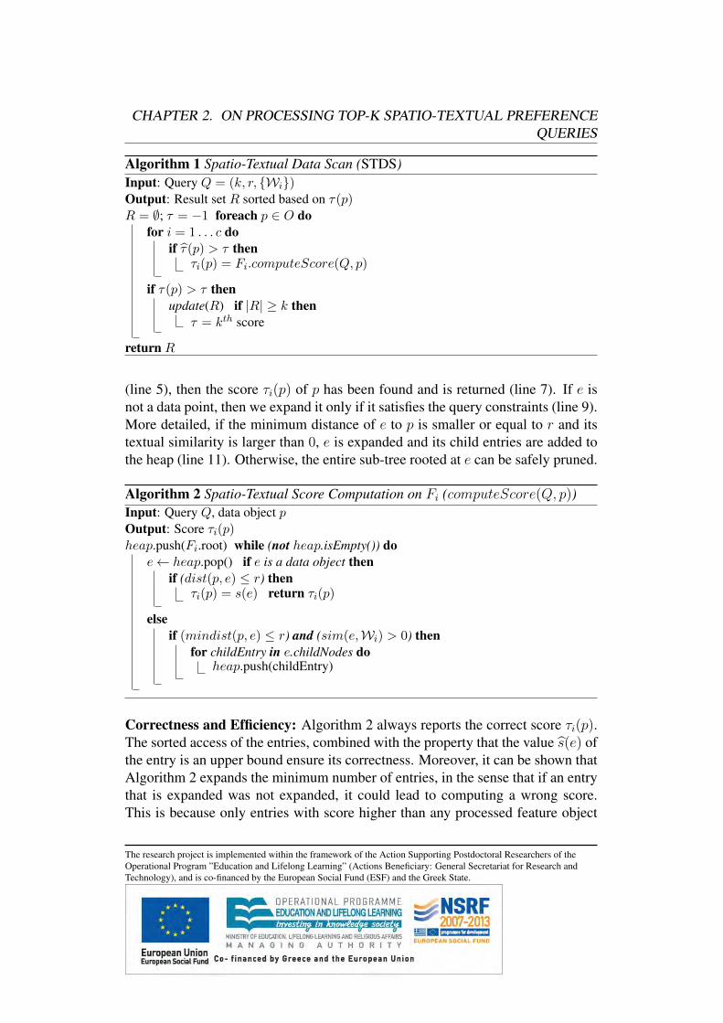
Algorithm 1 Spatio-Textual Data Scan (STDS)Input: Query Q = (k, r, {Wi})Output: Result set R sorted based on τ(p)R = ∅; τ = −1 foreach p ∈ O do
for i = 1 . . . c doif τ(p) > τ then
τi(p) = Fi.computeScore(Q, p)
if τ(p) > τ thenupdate(R) if |R| ≥ k then
τ = kth score
return R
(line 5), then the score τi(p) of p has been found and is returned (line 7). If e isnot a data point, then we expand it only if it satisfies the query constraints (line 9).More detailed, if the minimum distance of e to p is smaller or equal to r and itstextual similarity is larger than 0, e is expanded and its child entries are added tothe heap (line 11). Otherwise, the entire sub-tree rooted at e can be safely pruned.
Algorithm 2 Spatio-Textual Score Computation on Fi (computeScore(Q, p))Input: Query Q, data object pOutput: Score τi(p)heap.push(Fi.root) while (not heap.isEmpty()) do
e← heap.pop() if e is a data object thenif (dist(p, e) ≤ r) then
τi(p) = s(e) return τi(p)
elseif (mindist(p, e) ≤ r) and (sim(e,Wi) > 0) then
for childEntry in e.childNodes doheap.push(childEntry)
Correctness and Efficiency: Algorithm 2 always reports the correct score τi(p).The sorted access of the entries, combined with the property that the value s(e) ofthe entry is an upper bound ensure its correctness. Moreover, it can be shown thatAlgorithm 2 expands the minimum number of entries, in the sense that if an entrythat is expanded was not expanded, it could lead to computing a wrong score.This is because only entries with score higher than any processed feature object
The research project is implemented within the framework of the Action Supporting Postdoctoral Researchers of theOperational Program ”Education and Lifelong Learning” (Actions Beneficiary: General Secretariat for Research andTechnology), and is co-financed by the European Social Fund (ESF) and the Greek State.
CHAPTER 2. ON PROCESSING TOP-K SPATIO-TEXTUAL PREFERENCEQUERIES
are expanded, and such entries may contain in their sub-tree a feature object withscore equal to the score of the entry.Performance improvements: The performance of STDS can be improved byprocessing the score computations in a batch. Instead of a single data object p,a set of data objects P can be given as input to Algorithm 2. Then, an entry isexpanded if the distance for at least one p in P is smaller than r. When a featureobject is retrieved, for any p for which the distance is smaller than r the score iscomputed and those data objects p are removed from P . The same procedure isfollowed until either the heap orP is empty. Algorithm 1 can be easily modified toinvoke Algorithm 2 for all data objects in the same leaf entry of the R-tree (rtree)that indexes the data objects O. For sake of simplicity, we omit the implementa-tion details, even though we use this improved modification in our experimentalevaluation.
2.6 Spatio-Textual Preference Search (STPS)In this section we propose a novel and efficient algorithm, called Spatio-TextualPreference Search (STPS), for processing spatio-textual preference queries. STPSfollows a different strategy than STDS, as it involves two major steps, namelyfinding highly ranked feature objects first, and then, retrieving data objects intheir spatial neighborhood. Intuitively, if we find a neighborhood in which highlyranked feature objects exist, then the neighboring data objects are naturally highlyranked as well.
2.6.1 Valid Combination of Feature ObjectsIn a nutshell, the goal is to find sets of feature objects C = {t1, t2, . . . , tc} whereti ∈ Fi (1 ≤ i ≤ c), such that the spatio-textual preference score of each ti is ashigh as possible and the feature objects are located in nearby locations.
In the general case, a data object may be highly ranked even in the case wherea certain kind of feature object does not exist in its neighborhood, though fea-ture objects of other kinds might compensate for this. For example, consider theextreme case where all data objects have only one type of feature object in theirspatial neighborhood. For ease of presentation, we denote as ∅ a virtual featureobject for which it holds that dist(p, ∅) = 0, dist(ti, ∅) = 0 and s(∅) = 0 ∀ti, p.This virtual feature object is used for presenting unified definitions for the casewhere the spatio-textual score of the top-k data objects is defined based on less
The research project is implemented within the framework of the Action Supporting Postdoctoral Researchers of theOperational Program ”Education and Lifelong Learning” (Actions Beneficiary: General Secretariat for Research andTechnology), and is co-financed by the European Social Fund (ESF) and the Greek State.
CHAPTER 2. ON PROCESSING TOP-K SPATIO-TEXTUAL PREFERENCEQUERIES
Algorithm 3 Spatio-Textual Preference Search (STPS)Input: Query QOutput: Result set R sorted based on τ(p)while (|R| ≤ k) doC = nextCombination(Q) R = R∪ getDataObjects(C)
return R
than c feature objects. More formally put, we define the concept of valid combi-nation of feature objects as:
Definition 4 A valid combination of feature objects is a set C = {t1, t2, . . . , tc}such that (i) ∀i ti ∈ Fi or ti = ∅, and (ii) dist(ti, tj) ≤ 2r ∀i, j. The score of thevalid combination C is defined as s(C) =
∑1≤i≤c s(ti).
The following lemma proves that it is sufficient to examine only the validcombinations C of feature objects in order to retrieve the result set of a top-kspatio-textual preference query.
Lemma 1 The score of any data object p ∈ O is defined by a valid combinationof feature objects C = {t1, t2, . . . , tc}, i.e., ∀p : ∃C = {t1, t2, . . . , tc} such thatτ(p) = s(C)
Proof Let us assume that there exists p such that: τ(p) =∑
i∈[1,c] τi(p) withτi(p) = {s(ti) | ti ∈ Fi : dist(p, ti) ≤ r and sim(ti,Wi) > 0} and C ={t1, t2, . . . , tc} is not a valid combination of feature objects. Since C = {t1, t2, . . . , tc}is not a valid combination of feature objects, there exists 1 ≤ i 6= j ≤ c such thatdist(ti, tj) > 2r but also dist(p, ti) ≤ r and dist(p, tj) ≤ r. Based on the tri-angular inequality it holds: dist(ti, tj) ≤ dist(p, ti) + dist(p, tj) ≤ r + r ≤ 2r,which is a contradiction.
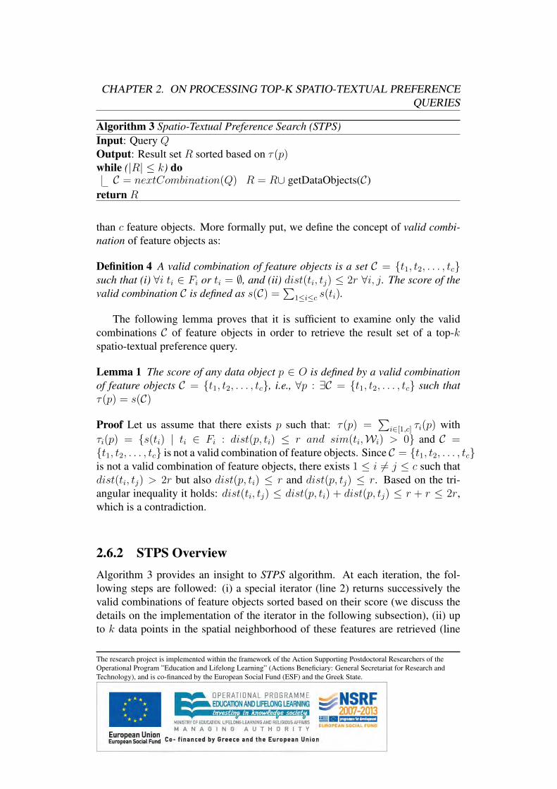
2.6.2 STPS OverviewAlgorithm 3 provides an insight to STPS algorithm. At each iteration, the fol-lowing steps are followed: (i) a special iterator (line 2) returns successively thevalid combinations of feature objects sorted based on their score (we discuss thedetails on the implementation of the iterator in the following subsection), (ii) upto k data points in the spatial neighborhood of these features are retrieved (line
The research project is implemented within the framework of the Action Supporting Postdoctoral Researchers of theOperational Program ”Education and Lifelong Learning” (Actions Beneficiary: General Secretariat for Research andTechnology), and is co-financed by the European Social Fund (ESF) and the Greek State.
CHAPTER 2. ON PROCESSING TOP-K SPATIO-TEXTUAL PREFERENCEQUERIES
3). Data objects that have already been previously retrieved are discarded, whilethe remaining data objects p have a score τ(p) = s(C) and can be returned tothe user incrementally. If k data objects have been returned to the user (line 1),the algorithm terminates without retrieving the remaining combinations of featureobjects. Differently to the STDS algorithm, STPS retrieves only the data objectsthat most certainly belong to the result set.
Algorithm 4 Spatio-Textual Feature Objects Retrieval (nextCombination(Q))Input: Query Qheapi: heap maintaining entries of Fi
heap: heap maintaining valid combinations of feature objectsDi: set of feature objects of Fi
Output: C: valid combination with highest scorewhile (∃i : not heapi.isEmpty()) do
i← nextFeatureSet() ei ← heapi.pop() while (not ei is a data object) dofor childEntry in ei.childNodes do
heapi.push(childEntry)ei ← heapi.pop()
Di = Di ∪ ei heap.push(validCombinations(D1, · · · ,ei ,· · · , Dc)) mini =s(ei) τ = max1≤j≤c(max1 + · · · + minj + · · · + maxc) C ← heap.top()if (score(C) ≥ τ ) then
heap.pop() return C
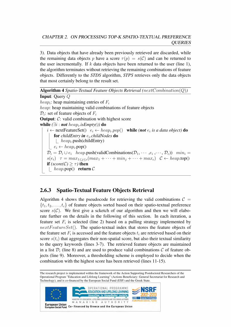
2.6.3 Spatio-Textual Feature Objects RetrievalAlgorithm 4 shows the pseudocode for retrieving the valid combinations C ={t1, t2, . . . , tc} of feature objects sorted based on their spatio-textual preferencescore s(C). We first give a scketch of our algorithm and then we will elabo-rate further on the details in the following of this section. In each iteration, afeature set Fi is selected (line 2) based on a pulling strategy implemented bynextFeatureSet(). The spatio-textual index that stores the feature objects ofthe feature set Fi is accessed and the feature objects ti are retrieved based on theirscore s(ti) that aggregates their non-spatial score, but also their textual similarityto the query keywords (lines 3-7). The retrieved feature objects are maintainedin a list Di (line 8) and are used to produce valid combinations C of feature ob-jects (line 9). Moreover, a thresholding scheme is employed to decide when thecombination with the highest score has been retrieved (lines 11-15).
The research project is implemented within the framework of the Action Supporting Postdoctoral Researchers of theOperational Program ”Education and Lifelong Learning” (Actions Beneficiary: General Secretariat for Research andTechnology), and is co-financed by the European Social Fund (ESF) and the Greek State.

CHAPTER 2. ON PROCESSING TOP-K SPATIO-TEXTUAL PREFERENCEQUERIES
We denote as maxi the maximum score of Di and mini the minimum scoreof Di. Thus, mini represents the best potential score of any feature object of Fi
that has not been processed yet. Moreover, in Algorithm 4 the variables heapi,Di, maxi, mini, and heap are global variables. They are initialized as followingheapi: the root of Fi, Di = ∅ and heap = ∅, mini = ∞. Variable maxi is thescore of the highest ranked feature object of Fi and is set the first time the Fi indexis accessed.Accessing Fi: In each iteration, Algorithm 4 accesses one spatio-textual index thatstores the set Fi (lines 3-7). The entries of the spatio-textual index responsible forthe feature objects of Fi are maintained in heapi, which keeps the entries e sortedbased on s(e). Moreover, for sake of simplicity, we assume that heapi.pop() willreturn a virtual feature object ti = ∅ (with score equal to 0) as final object. In eachiteration an entry ei of the spatio-textual index is retrieved from heapi (line 3). Ifthe entry ei corresponds to a node of the index, the entry is expanded and its childnodes are added to the heapi (lines 5-6). Algorithm 4 continues retrieving fromheapi entries, until an entry that is a feature object is retrieved (line 4). When anentry ei is retrieved that corresponds to a feature object, ei is inserted in the listDi
(line 8).Creation of C: After retrieving a new feature object ei, new valid combinationsC are created by combining ei with the previously retrieved feature objects tjmaintained in the lists Dj (line 9). For this, the method validCombinations iscalled, which returns all combinations of the objects in Dj and ei, by discardingcombinations for which the condition dist(ti, tj) ≤ 2r ∀i, j does not hold. Thenew valid combinations are inserted in the heap (line 9) that maintains the validcombinations sorted based on their score s(C).Thresholding scheme: Algorithm 4 employs a thresholding scheme to determineif the current best valid combination can be returned as the valid combinationwith the highest score. The threshold τ represents the best score of any validcombination of feature objects that has not been examined yet. The best scoreof the next feature object tj retrieved from Fj is equal to minj , since the featureobjects are accessed sorted based on s(tj). Obviously, for the remaining featuresets we assume that the new feature object tj is combined with the feature objectsthat have the highest score. Thus, τ = max1≤j≤c(max1+· · ·+minj+· · ·+maxc)(line 11) is an upper bound of the score for any valid combination that has notbeen examined yet. In line 13, we test whether the best combination of featureobjects in the heap has a score higher or equal to the threshold τ . If so, thebest combination in the heap is the next valid combination with the best score.Otherwise, additional feature objects from feature sets Fi have to be retrieved
The research project is implemented within the framework of the Action Supporting Postdoctoral Researchers of theOperational Program ”Education and Lifelong Learning” (Actions Beneficiary: General Secretariat for Research andTechnology), and is co-financed by the European Social Fund (ESF) and the Greek State.

CHAPTER 2. ON PROCESSING TOP-K SPATIO-TEXTUAL PREFERENCEQUERIES
until it holds that the top element of the heap achieves a score which is higherthan τ .Pulling strategy: In the following, we proposed an advanced pulling strategy thatprioritizes retrieval from feature sets that have higher potential to produce the nextvalid combination C. A simple alternative would be to access the different featuresets in a round robin fashion.
The order in which the feature objects of different feature sets are retrieved isdefined by a pulling strategy, i.e., nextFeatureSet() returns an integer between1 and c and defines the pulling strategy. In addition, nextFeatureSet() neverreturns i if heapi is empty.
Definition 5 Given c sets of feature objects Di, the prioritized pulling strategyreturns m as the next feature set such that τ = max1 + · · ·+minm + · · ·+maxc.
The main idea of the prioritized pulling strategy is that in each iteration thefeature set Fm that is responsible for the threshold value τ is accessed. It is obvi-ous that the only way to reduce τ is to reduce the minm, since retrieval from theremaining feature sets cannot reduce τ . Thus, retrieving the next tuple from thefeature set Fm may reduce the threshold τ and may produce new valid combina-tions that have a score equal to the current threshold.
2.6.4 Retrieval of Qualified Data ObjectsIn the following, we study the reciprocal actions taken upon the formation of ahighly ranked combination of feature objects.
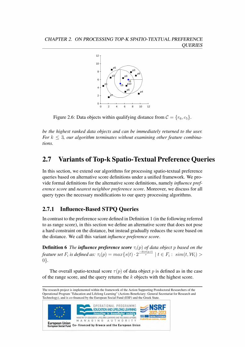
In Algorithm 3 (line 3) getObjects(C) is invoked to retrieve from rtree all dataobjects in the neighborhood of the feature objects in C. This method starts fromthe root of the rtree and processes its entries recursively. Entries e for which ∃isuch that ti ∈ C with dist(e, ti) > r are discarded. The remaining entries areexpanded until all objects p for which it holds that dist(p, ti) ≤ r are retrieved.Example. Consider for example the feature sets depicted in Figure 2.2 and inFigure 2.3. Given a query with r = 3.5, W1 = {italian, pizza} and W2 ={espresso, muffins}, the restaurant and the coffeehouse with the highest scoresare r6 and c5 respectively. Since it holds that dist(r6, c5) ≤ 2r, the set C ={r6, c5} is a valid combination of feature objects. Assume that the set of data ob-jects isO = {p1, p2, . . . , p10} as depicted in Figure 2.6. For the data objects p6, p9
and p10 it holds that dist(pi, c5) ≤ r and dist(pi, r6) ≤ r, and their spatial-textualscore is τ(p6) = τ(p9) = τ(p10) = 1.6833. These data objects are guaranteed to
The research project is implemented within the framework of the Action Supporting Postdoctoral Researchers of theOperational Program ”Education and Lifelong Learning” (Actions Beneficiary: General Secretariat for Research andTechnology), and is co-financed by the European Social Fund (ESF) and the Greek State.
CHAPTER 2. ON PROCESSING TOP-K SPATIO-TEXTUAL PREFERENCEQUERIES
0
2
4
6
8
10
12
0 2 4 6 8 10 12
c5
r6p1
p2
p3
p4
p5
p6
p7
p8p9
p10
Figure 2.6: Data objects within qualifying distance from C = {r6, c5}.
be the highest ranked data objects and can be immediately returned to the user.For k ≤ 3, our algorithm terminates without examining other feature combina-tions.
2.7 Variants of Top-k Spatio-Textual Preference QueriesIn this section, we extend our algorithms for processing spatio-textual preferencequeries based on alternative score definitions under a unified framework. We pro-vide formal definitions for the alternative score definitions, namely influence pref-erence score and nearest neighbor preference score. Moreover, we discuss for allquery types the necessary modifications to our query processing algorithms.
2.7.1 Influence-Based STPQ QueriesIn contrast to the preference score defined in Definition 1 (in the following referredto as range score), in this section we define an alternative score that does not posea hard constraint on the distance, but instead gradually reduces the score based onthe distance. We call this variant influence preference score.
Definition 6 The influence preference score τi(p) of data object p based on thefeature set Fi is defined as: τi(p) = max{s(t) · 2
−dist(p,t)r | t ∈ Fi : sim(t,Wi) >
0}.
The overall spatio-textual score τ(p) of data object p is defined as in the caseof the range score, and the query returns the k objects with the highest score.
The research project is implemented within the framework of the Action Supporting Postdoctoral Researchers of theOperational Program ”Education and Lifelong Learning” (Actions Beneficiary: General Secretariat for Research andTechnology), and is co-financed by the European Social Fund (ESF) and the Greek State.
CHAPTER 2. ON PROCESSING TOP-K SPATIO-TEXTUAL PREFERENCEQUERIES
The STDS algorithm, as defined in Algorithm 1 can be easily adapted for thecase of influence score. Only the function computeScore(Q, p) must be modifiedaccording to the definition of the score variant. Thus, in Algorithm 2 each entry inline 2.5 will be prioritized according to the influence preference score. In addition,the range restriction is removed in line 5 and line 9. No further modifications areneeded, thus in the following we focus on the modifications and optimizationsneeded for STPS algorithm.
Algorithm 5 STPS for influence scoreInput: Query QOutput: Result set R sorted based on τ(p)τ = 0 score = −1 while (|R| ≤ k) or (best ¿ τ ) doC = nextCombination(Q) best = s(C) R = R∪ getDataObjects(C) τ =k-th score in R
return R
STPQ queries based on the influence preference score can be efficiently sup-ported by the STPS algorithm with few modifications. Algorithm 5 shows themodified STPS for influence preference score. The algorithm continues until atleast k data object have been retrieved and until we are sure that none of the re-maining data objects can have a better score. We use the score of the k-th dataobject of the current top-k result (line 7) to set a threshold τ . Hence, if the bestscore of any unseen combination is smaller or equal to τ , the algorithm natu-rally terminates. In more details, C = nextCombination(Q) is the same withAlgorithm 4 and returns the best combination based on score s(C), but withoutdiscarding combinations whose distance is greater than 2r. Thus, in each iterationthe combination C with the highest τ(p) =
∑i∈[1,c] τi(p) is retrieved. Recall that
for the case of the range preference score, all data objects that were located indistance smaller than r from all feature objects of C had a score equal to s(C).Instead in the case of the influence preference score, s(C) is an upper bound forthe score of all data objects based on C. This is because, the computed score isthe influence score only for the objects with distance 0, while all other objectshave a smaller influence score. Therefore, getDataObjects(C) must be modifiedaccordingly.
In more details, getDataObjects() retrieves the k points that have the high-est influence score, by starting a top-k query on the R-Tree (rtree) of the dataobjects. The root is inserted in a heap sorted by the influence score (τ(p) =∑
i∈[1,c] τi(p)2−dist(p,ti)
r ). For non-leaf entries e the influence score is computed
The research project is implemented within the framework of the Action Supporting Postdoctoral Researchers of theOperational Program ”Education and Lifelong Learning” (Actions Beneficiary: General Secretariat for Research andTechnology), and is co-financed by the European Social Fund (ESF) and the Greek State.
CHAPTER 2. ON PROCESSING TOP-K SPATIO-TEXTUAL PREFERENCEQUERIES
based on the mindist. Then, the influence score of an entry is an upper boundof any object in the subtree. After retrieving k data objects, we have retrievedthe k data objects with the highest influence score for this combination of fea-ture objects. Further improvement can be achieved if getDataObjects() stopsretrieving data objects based on τ , which reduces the I/Os on rtree. If τ is givento getDataObjects() then it will return at most k data objects that have a scoresmaller than τ . Line 6 merges the results while it removes objects that have beenretrieved before. Thus, if an object that is already in the heap is retrieved againthe score with the highest value is kept.
After retrieving k data objects with the highest τ(p) in line 6 (Algorithm 5),the score of the k-th data object in R is used as a threshold τ (line 7). The bestscore of any unseen combination is best = s(C), which is also an upper bound forthe score of any unseen data object, since this is the score for distance 0. Hence,if the best score is greater than τ , we have to retrieve additional objects. If thescore s(C) of the next combination is smaller than or equal to the threshold westop retrieving other combinations.
2.7.2 Nearest Neighbor STPQ QueriesIn the next score variant, each data object takes as a score the goodness of thefeature objects that are its nearest neighbors. In particular, for each feature set thescore of the nearest feature object is considered for computing the score of a dataobject.
Definition 7 The nearest neighbor preference score τi(p) of data object p basedon the feature set Fi is defined as: τi(p) = {s(t) | t ∈ Fi : dist(p, t) ≤dist(p, t′) ∀t′ ∈ Fi and sim(t,Wi) > 0}
The overall spatio-textual score τ(p) of data object p is defined as in the caseof the range score, and the query returns the k objects with the highest score.Again, STDS treats nearest neighbor queries similarly as in Algorithm 2 with sub-tle changes. The range predicate is removed in line 5 and line 9, while the childentries are prioritized in the heap according to their minimum distance from thedata object p.
Regarding STPS, Algorithm 3 is directly applicable for the nearest neighborscore by modifying nextCombination(Q) of Algorithm 4 to return the best com-bination based on score s(), but without discarding combinations that have a
The research project is implemented within the framework of the Action Supporting Postdoctoral Researchers of theOperational Program ”Education and Lifelong Learning” (Actions Beneficiary: General Secretariat for Research andTechnology), and is co-financed by the European Social Fund (ESF) and the Greek State.
CHAPTER 2. ON PROCESSING TOP-K SPATIO-TEXTUAL PREFERENCEQUERIES
distance > 2r, as also in the case of the influence score. The remaining chal-lenge is given a combination C to retrieve the data objects that satisfy the nearestneighbor requirement.
Generally, it is more difficult compared to the other score variants to retrievethe data objects for a given combination C. We need to retrieve all data objects forwhich the nearest neighbor ti based on Fi belongs to C. For each feature object tiof C, there exists a region in which all data points that fall into that region have tias their nearest neighbor. This region corresponds to the Voronoi cell [34] and thisproblem has been studied for finding reverse nearest neighbors [26]. Only the dataobjects in the intersection of all regions need to be retrieved. In fact, we computeincrementally the Voronoi cell for each feature object ti of C, which allows us todiscard early combinations for which the intersection becomes empty. We omitfurther implementation details due to space limitations.
2.8 Experimental EvaluationIn this section, we evaluate the performance of our algorithms STDS and STPS,presented previously in Section 2.5 and Section 2.6 respectively, for processingspatio-textual preference queries over large disk-resident data. Moreover, westudy the gains in performance of our algorithms caused by the SRT index pro-posed in Section 2.4 compared to an existing indexing technique (IR2-Tree [17]).In order to ensure a fair comparison, we modify the IR2-Tree to support scorevalues of feature objects. To this end, we add to the leaf nodes of IR2-Tree thescoring values for the feature objects, and maintain in ancestor (internal) nodesthe maximum score of all enclosed feature objects. All experiments run on anIntel 2.2GHz processor equipped with 2GB RAM.
2.8.1 Experimental SetupMethodology. In our experimental evaluation, we vary four important parametersof the datasets in order to study the scalability of the proposed techniques (Sec-tion 2.8.2). These parameters are: (i) the cardinality of the feature sets |Fi|, (ii)the cardinality of the set of data objects |O|, (iii) the number of feature sets c,and (iv) number of distinct keywords indexed. Moreover, we study four differ-ent query parameters to study how the characteristics of the query influence theperformance of the algorithms (Section 2.8.3). In more details, we vary (i) thequery radius r, (ii) the number k of retrieved data objects, (iii) the smoothing pa-
The research project is implemented within the framework of the Action Supporting Postdoctoral Researchers of theOperational Program ”Education and Lifelong Learning” (Actions Beneficiary: General Secretariat for Research andTechnology), and is co-financed by the European Social Fund (ESF) and the Greek State.
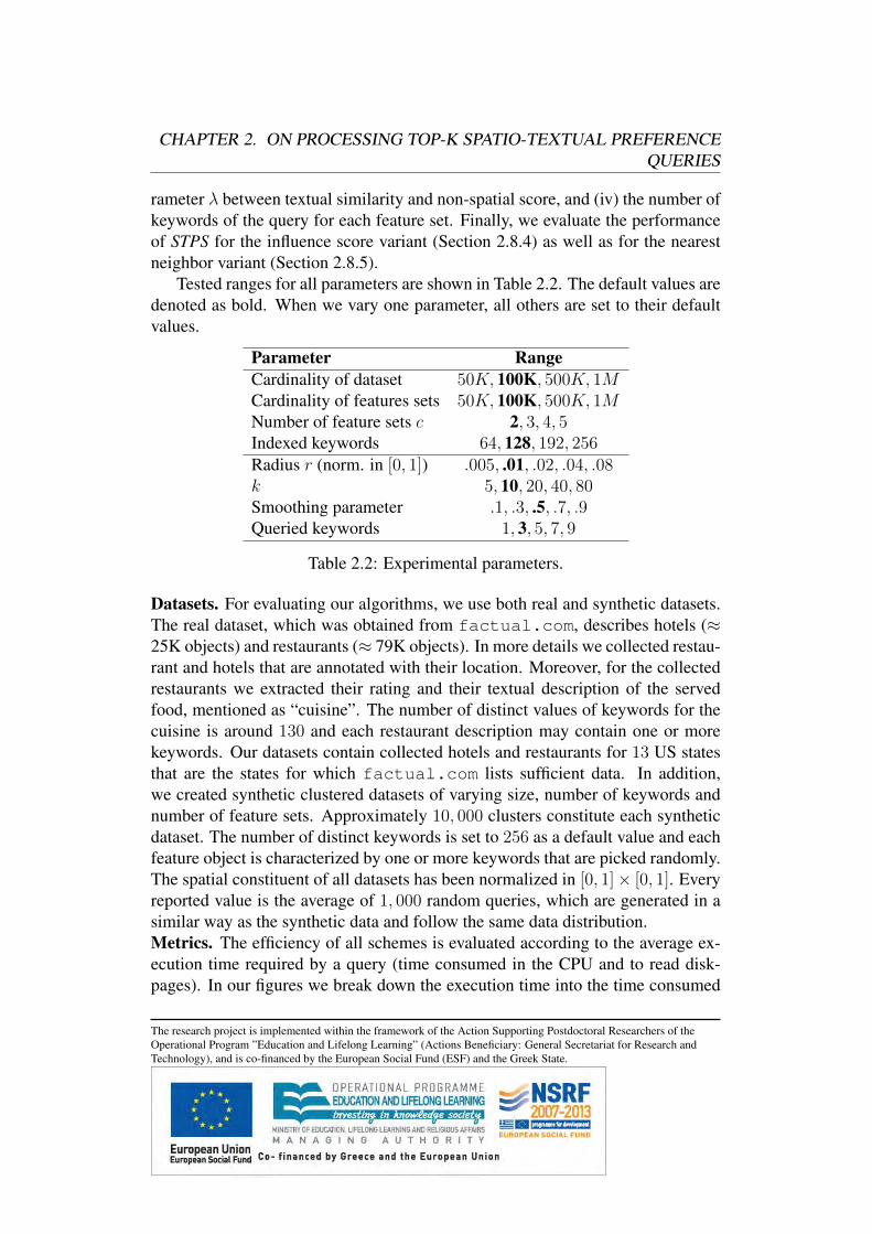
CHAPTER 2. ON PROCESSING TOP-K SPATIO-TEXTUAL PREFERENCEQUERIES
rameter λ between textual similarity and non-spatial score, and (iv) the number ofkeywords of the query for each feature set. Finally, we evaluate the performanceof STPS for the influence score variant (Section 2.8.4) as well as for the nearestneighbor variant (Section 2.8.5).
Tested ranges for all parameters are shown in Table 2.2. The default values aredenoted as bold. When we vary one parameter, all others are set to their defaultvalues.
Parameter RangeCardinality of dataset 50K, 100K, 500K, 1MCardinality of features sets 50K, 100K, 500K, 1MNumber of feature sets c 2, 3, 4, 5Indexed keywords 64, 128, 192, 256Radius r (norm. in [0, 1]) .005, .01, .02, .04, .08k 5, 10, 20, 40, 80Smoothing parameter .1, .3, .5, .7, .9Queried keywords 1, 3, 5, 7, 9
Table 2.2: Experimental parameters.
Datasets. For evaluating our algorithms, we use both real and synthetic datasets.The real dataset, which was obtained from factual.com, describes hotels (≈25K objects) and restaurants (≈ 79K objects). In more details we collected restau-rant and hotels that are annotated with their location. Moreover, for the collectedrestaurants we extracted their rating and their textual description of the servedfood, mentioned as “cuisine”. The number of distinct values of keywords for thecuisine is around 130 and each restaurant description may contain one or morekeywords. Our datasets contain collected hotels and restaurants for 13 US statesthat are the states for which factual.com lists sufficient data. In addition,we created synthetic clustered datasets of varying size, number of keywords andnumber of feature sets. Approximately 10, 000 clusters constitute each syntheticdataset. The number of distinct keywords is set to 256 as a default value and eachfeature object is characterized by one or more keywords that are picked randomly.The spatial constituent of all datasets has been normalized in [0, 1]× [0, 1]. Everyreported value is the average of 1, 000 random queries, which are generated in asimilar way as the synthetic data and follow the same data distribution.Metrics. The efficiency of all schemes is evaluated according to the average ex-ecution time required by a query (time consumed in the CPU and to read disk-pages). In our figures we break down the execution time into the time consumed
The research project is implemented within the framework of the Action Supporting Postdoctoral Researchers of theOperational Program ”Education and Lifelong Learning” (Actions Beneficiary: General Secretariat for Research andTechnology), and is co-financed by the European Social Fund (ESF) and the Greek State.
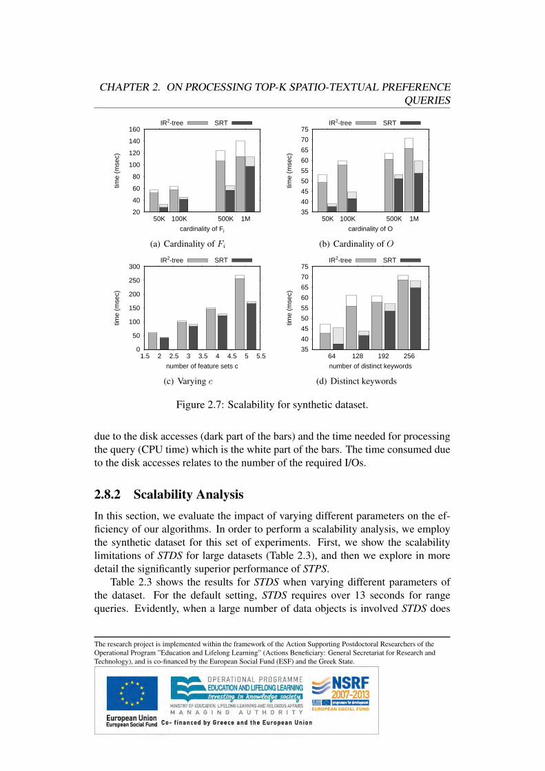
CHAPTER 2. ON PROCESSING TOP-K SPATIO-TEXTUAL PREFERENCEQUERIES
20
40
60
80
100
120
140
160
50K 100K 500K 1M
time
(mse
c)
cardinality of Fi
IR2-tree SRT
(a) Cardinality of Fi
35
40
45
50
55
60
65
70
75
50K 100K 500K 1M
time
(mse
c)
cardinality of O
IR2-tree SRT
(b) Cardinality of O
0
50
100
150
200
250
300
1.5 2 2.5 3 3.5 4 4.5 5 5.5
time
(mse
c)
number of feature sets c
IR2-tree SRT
(c) Varying c
35
40
45
50
55
60
65
70
75
64 128 192 256
time
(mse
c)
number of distinct keywords
IR2-tree SRT
(d) Distinct keywords
Figure 2.7: Scalability for synthetic dataset.
due to the disk accesses (dark part of the bars) and the time needed for processingthe query (CPU time) which is the white part of the bars. The time consumed dueto the disk accesses relates to the number of the required I/Os.
2.8.2 Scalability AnalysisIn this section, we evaluate the impact of varying different parameters on the ef-ficiency of our algorithms. In order to perform a scalability analysis, we employthe synthetic dataset for this set of experiments. First, we show the scalabilitylimitations of STDS for large datasets (Table 2.3), and then we explore in moredetail the significantly superior performance of STPS.
Table 2.3 shows the results for STDS when varying different parameters ofthe dataset. For the default setting, STDS requires over 13 seconds for rangequeries. Evidently, when a large number of data objects is involved STDS does
The research project is implemented within the framework of the Action Supporting Postdoctoral Researchers of theOperational Program ”Education and Lifelong Learning” (Actions Beneficiary: General Secretariat for Research andTechnology), and is co-financed by the European Social Fund (ESF) and the Greek State.
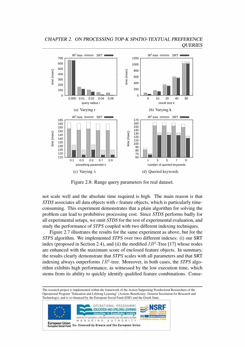
CHAPTER 2. ON PROCESSING TOP-K SPATIO-TEXTUAL PREFERENCEQUERIES
0
100
200
300
400
500
600
700
0.005 0.01 0.02 0.04 0.08
time
(mse
c)
query radius r
IR2-tree SRT
(a) Varying r
0
200
400
600
800
1000
1200
5 10 20 40 80
time
(mse
c)
result size k
IR2-tree SRT
(b) Varying k
115 120 125 130 135 140 145 150 155 160 165
0.1 0.3 0.5 0.7 0.9
time
(mse
c)
smoothing parametel λ
IR2-tree SRT
(c) Varying λ
60 70 80 90
100 110 120 130 140 150 160 170
1 3 5 7 9
time
(mse
c)
number of queried keywords
IR2-tree SRT
(d) Queried keywords
Figure 2.8: Range query parameters for real dataset.
not scale well and the absolute time required is high. The main reason is thatSTDS associates all data objects with c feature objects, which is particularly time-consuming. This experiment demonstrates that a plain algorithm for solving theproblem can lead to prohibitive processing cost. Since STDS performs badly forall experimental setups, we omit STDS for the rest of experimental evaluation, andstudy the performance of STPS coupled with two different indexing techniques.
Figure 2.7 illustrates the results for the same experiment as above, but for theSTPS algorithm. We implemented STPS over two different indexes: (i) our SRTindex (proposed in Section 2.4), and (ii) the modified IR2-Tree [17] whose nodesare enhanced with the maximum score of enclosed feature objects. In summary,the results clearly demonstrate that STPS scales with all parameters and that SRTindexing always outperforms IR2-tree. Moreover, in both cases, the STPS algo-rithm exhibits high performance, as witnessed by the low execution time, whichstems from its ability to quickly identify qualified feature combinations. Conse-
The research project is implemented within the framework of the Action Supporting Postdoctoral Researchers of theOperational Program ”Education and Lifelong Learning” (Actions Beneficiary: General Secretariat for Research andTechnology), and is co-financed by the European Social Fund (ESF) and the Greek State.
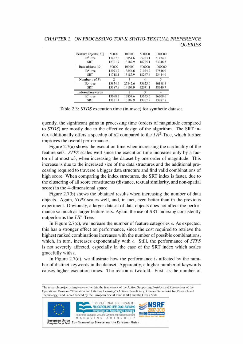
CHAPTER 2. ON PROCESSING TOP-K SPATIO-TEXTUAL PREFERENCEQUERIES
Feature objects |Fi| 50000 100000 500000 1000000IR2-tree 13427.3 13854.6 25223.1 31434.6
SRT 12301.7 13187.9 18725.1 23046.3Data objects |O| 50000 100000 500000 1000000
IR2-tree 13073.2 13854.6 21074.2 27846.0SRT 11718.1 13187.9 18267.4 23444.9
Number c of Fi 2 3 4 5IR2-tree 13854.6 27842.6 33625.0 40188.4
SRT 13187.9 14104.9 32071.1 38340.7Indexed keywords 1 2 3 4
IR2-tree 13698.7 13854.6 15655.6 16209.6SRT 13121.4 13187.9 13207.9 13887.8
Table 2.3: STDS execution time (in msec) for synthetic dataset.
quently, the significant gains in processing time (orders of magnitude comparedto STDS) are mostly due to the effective design of the algorithm. The SRT in-dex additionally offers a speedup of x2 compared to the IR2-Tree, which furtherimproves the overall performance.
Figure 2.7(a) shows the execution time when increasing the cardinality of thefeature sets. STPS scales well since the execution time increases only by a fac-tor of at most x3, when increasing the dataset by one order of magnitude. Thisincrease is due to the increased size of the data structures and the additional pro-cessing required to traverse a bigger data structure and find valid combinations ofhigh score. When comparing the index structures, the SRT index is faster, due tothe clustering of all score constituents (distance, textual similarity, and non-spatialscore) in the 4-dimensional space.
Figure 2.7(b) shows the obtained results when increasing the number of dataobjects. Again, STPS scales well, and, in fact, even better than in the previousexperiment. Obviously, a larger dataset of data objects does not affect the perfor-mance so much as larger feature sets. Again, the use of SRT indexing consistentlyoutperforms the IR2-Tree.
In Figure 2.7(c), we increase the number of feature categories c. As expected,this has a stronger effect on performance, since the cost required to retrieve thehighest ranked combinations increases with the number of possible combinations,which, in turn, increases exponentially with c. Still, the performance of STPSis not severely affected, especially in the case of the SRT index which scalesgracefully with c.
In Figure 2.7(d), we illustrate how the performance is affected by the num-ber of distinct keywords in the dataset. Apparently, a higher number of keywordscauses higher execution times. The reason is twofold. First, as the number of
The research project is implemented within the framework of the Action Supporting Postdoctoral Researchers of theOperational Program ”Education and Lifelong Learning” (Actions Beneficiary: General Secretariat for Research andTechnology), and is co-financed by the European Social Fund (ESF) and the Greek State.
CHAPTER 2. ON PROCESSING TOP-K SPATIO-TEXTUAL PREFERENCEQUERIES
distinct keywords increases, it is less probable to find feature objects that are de-scribed by all queried keywords, thus more feature objects need to be retrievedin order to ensure that no other combination has a higher score. Secondly, thenode capacity of the index structures drops, thus the height of the index structuresmay increase, thus causing more IOs. In any case, the increase in the absolutevalue of execution time is relatively small (20 msec), even when we increase thevocabulary by a factor of 4 (from 64 to 256 keywords).
2.8.3 Varying Query ParametersIn Figure 2.8, we study the effect of varying query parameters for the real dataset.First, in Figure 2.8(a), we evaluate the impact of increasing the query radius ron the performance of STPS. We notice that for smaller values of r the executiontime increases and the gain of SRT indexing compared to IR2-tree drops. Forsmall radius, access to more qualified combinations of feature objects is required,since only few data objects are located in their neighborhood. Therefore, for bothindexing approaches the execution time increases mainly due to the increase ofthe IOs. Since a high percentage of the feature objects need to be retrieved foreach feature set, the gain of SRT indexing is small. However, difference in perfor-mance becomes obvious for greater values of r, and hence, finding relevant featureobjects in terms of textual description and good non-spatial score becomes mostimportant for accessing only few feature objects.
Figure 2.8(b) illustrates the execution time when varying the size of result setk. Overall, the execution time increases as k increases. Specifically, with highervalues of k more combinations of feature objects are retrieved to compose theresult set, which again lead to more IOs to retrieve the qualifying feature objectsthat constitute valid combinations.
In Figure 2.8(c), we vary the smoothing parameter λ. In general, both ap-proaches exhibit relatively stable performance for varying values of λ. The per-formance of IR2-tree is not affected by the smoothing parameter, since the featureobjects are not grouped into blocks based on the non-spatial score nor based ontheir textual similarity. We note for the IR2-tree that objects with similar textualdescriptions are stored throughout the index, regardless of their non-spatial score;unlike the SRT index where they are clustered together in the same block. Asa result, a significant overhead is evident when searching for relevant objects allover the IR2-tree. On the other hand, the SRT index is built by taking into accountnon-spatial score, the textual information and the spatial location. Thus, STPSthat uses SRT index is consistently more efficient regardless of the value of the
The research project is implemented within the framework of the Action Supporting Postdoctoral Researchers of theOperational Program ”Education and Lifelong Learning” (Actions Beneficiary: General Secretariat for Research andTechnology), and is co-financed by the European Social Fund (ESF) and the Greek State.
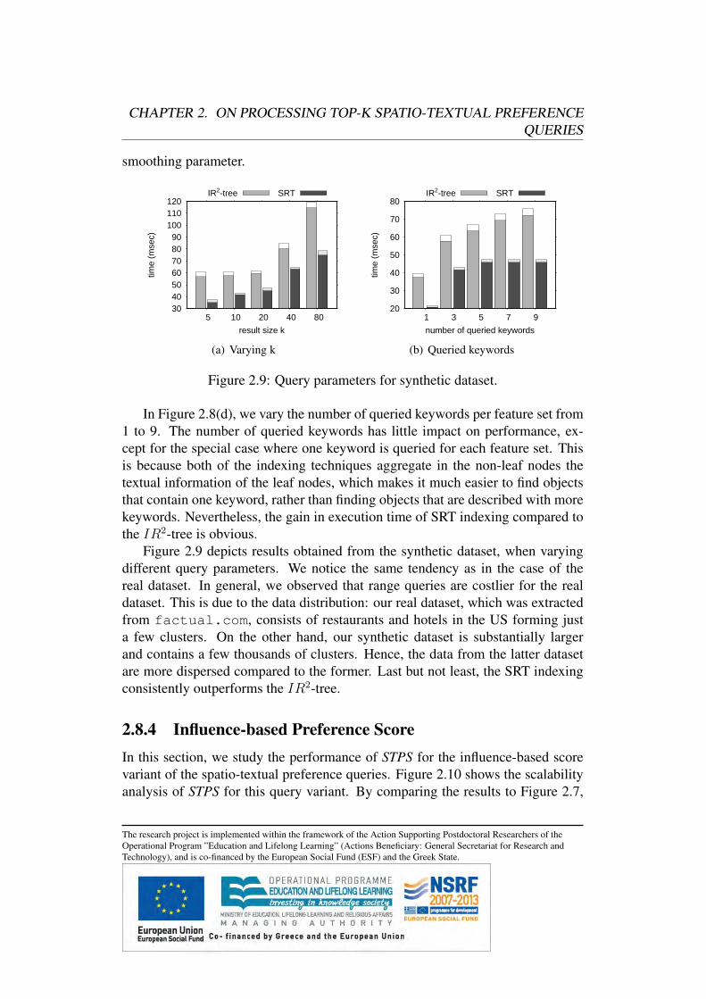
CHAPTER 2. ON PROCESSING TOP-K SPATIO-TEXTUAL PREFERENCEQUERIES
smoothing parameter.
30 40 50 60 70 80 90
100 110 120
5 10 20 40 80
time
(mse
c)
result size k
IR2-tree SRT
(a) Varying k
20
30
40
50
60
70
80
1 3 5 7 9
time
(mse
c)
number of queried keywords
IR2-tree SRT
(b) Queried keywords
Figure 2.9: Query parameters for synthetic dataset.
In Figure 2.8(d), we vary the number of queried keywords per feature set from1 to 9. The number of queried keywords has little impact on performance, ex-cept for the special case where one keyword is queried for each feature set. Thisis because both of the indexing techniques aggregate in the non-leaf nodes thetextual information of the leaf nodes, which makes it much easier to find objectsthat contain one keyword, rather than finding objects that are described with morekeywords. Nevertheless, the gain in execution time of SRT indexing compared tothe IR2-tree is obvious.
Figure 2.9 depicts results obtained from the synthetic dataset, when varyingdifferent query parameters. We notice the same tendency as in the case of thereal dataset. In general, we observed that range queries are costlier for the realdataset. This is due to the data distribution: our real dataset, which was extractedfrom factual.com, consists of restaurants and hotels in the US forming justa few clusters. On the other hand, our synthetic dataset is substantially largerand contains a few thousands of clusters. Hence, the data from the latter datasetare more dispersed compared to the former. Last but not least, the SRT indexingconsistently outperforms the IR2-tree.
2.8.4 Influence-based Preference ScoreIn this section, we study the performance of STPS for the influence-based scorevariant of the spatio-textual preference queries. Figure 2.10 shows the scalabilityanalysis of STPS for this query variant. By comparing the results to Figure 2.7,
The research project is implemented within the framework of the Action Supporting Postdoctoral Researchers of theOperational Program ”Education and Lifelong Learning” (Actions Beneficiary: General Secretariat for Research andTechnology), and is co-financed by the European Social Fund (ESF) and the Greek State.
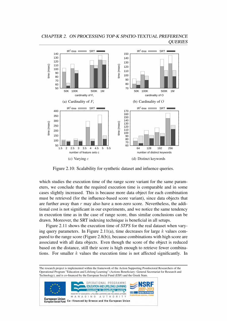
CHAPTER 2. ON PROCESSING TOP-K SPATIO-TEXTUAL PREFERENCEQUERIES
50 60 70 80 90
100 110 120 130 140
50K 100K 500K 1M
time
(mse
c)
cardinality of Fi
IR2-tree SRT
(a) Cardinality of Fi
70
80
90
100
110
120
130
140
150
50K 100K 500K 1M
time
(mse
c)
cardinality of O
IR2-tree SRT
(b) Cardinality of O
50
100
150
200
250
300
350
400
1.5 2 2.5 3 3.5 4 4.5 5 5.5
time
(mse
c)
number of feature sets c
IR2-tree SRT
(c) Varying c
60 70 80 90
100 110 120 130 140 150 160 170
64 128 192 256
time
(mse
c)
number of distinct keywords
IR2-tree SRT
(d) Distinct keywords
Figure 2.10: Scalability for synthetic dataset and infuence queries.
which studies the execution time of the range score variant for the same param-eters, we conclude that the required execution time is comparable and in somecases slightly increased. This is because more data object for each combinationmust be retrieved (for the influence-based score variant), since data objects thatare further away than r may also have a non-zero score. Nevertheless, the addi-tional cost is not significant in our experiments, and we notice the same tendencyin execution time as in the case of range score, thus similar conclusions can bedrawn. Moreover, the SRT indexing technique is beneficial in all setups.
Figure 2.11 shows the execution time of STPS for the real dataset when vary-ing query parameters. In Figure 2.11(a), time decreases for large k values com-pared to the range score (Figure 2.8(b)), because combinations with high score areassociated with all data objects. Even though the score of the object is reducedbased on the distance, still their score is high enough to retrieve fewer combina-tions. For smaller k values the execution time is not affected significantly. In
The research project is implemented within the framework of the Action Supporting Postdoctoral Researchers of theOperational Program ”Education and Lifelong Learning” (Actions Beneficiary: General Secretariat for Research andTechnology), and is co-financed by the European Social Fund (ESF) and the Greek State.
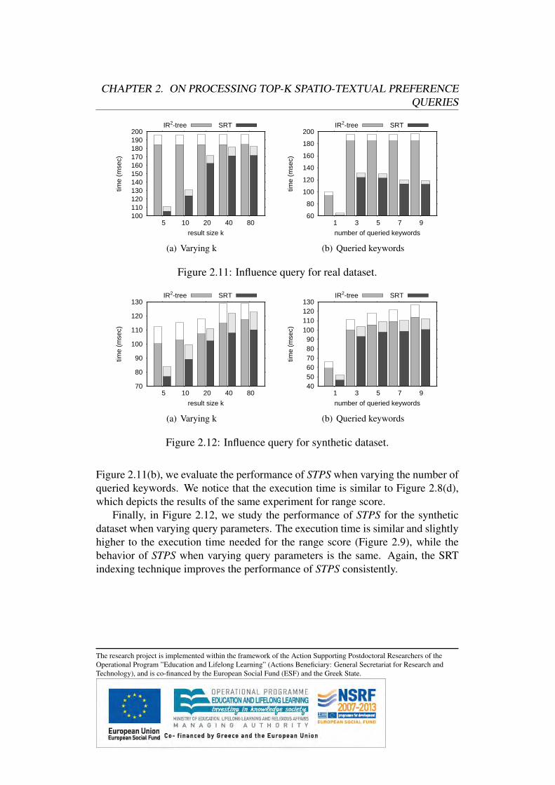
CHAPTER 2. ON PROCESSING TOP-K SPATIO-TEXTUAL PREFERENCEQUERIES
100 110 120 130 140 150 160 170 180 190 200
5 10 20 40 80
time
(mse
c)
result size k
IR2-tree SRT
(a) Varying k
60
80
100
120
140
160
180
200
1 3 5 7 9
time
(mse
c)
number of queried keywords
IR2-tree SRT
(b) Queried keywords
Figure 2.11: Influence query for real dataset.
70
80
90
100
110
120
130
5 10 20 40 80
time
(mse
c)
result size k
IR2-tree SRT
(a) Varying k
40 50 60 70 80 90
100 110 120 130
1 3 5 7 9
time
(mse
c)
number of queried keywords
IR2-tree SRT
(b) Queried keywords
Figure 2.12: Influence query for synthetic dataset.
Figure 2.11(b), we evaluate the performance of STPS when varying the number ofqueried keywords. We notice that the execution time is similar to Figure 2.8(d),which depicts the results of the same experiment for range score.
Finally, in Figure 2.12, we study the performance of STPS for the syntheticdataset when varying query parameters. The execution time is similar and slightlyhigher to the execution time needed for the range score (Figure 2.9), while thebehavior of STPS when varying query parameters is the same. Again, the SRTindexing technique improves the performance of STPS consistently.
The research project is implemented within the framework of the Action Supporting Postdoctoral Researchers of theOperational Program ”Education and Lifelong Learning” (Actions Beneficiary: General Secretariat for Research andTechnology), and is co-financed by the European Social Fund (ESF) and the Greek State.
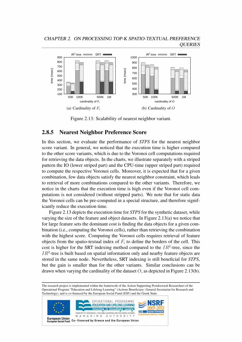
CHAPTER 2. ON PROCESSING TOP-K SPATIO-TEXTUAL PREFERENCEQUERIES
100
200
300
400
500
600
700
800
900
50K 100K 500K 1M
time
(mse
c)
cardinality of Fi
IR2-tree SRT
(a) Cardinality of Fi
300
400
500
600
700
800
900
1000
50K 100K 500K 1M
time
(mse
c)
cardinality of O
IR2-tree SRT
(b) Cardinality of O
Figure 2.13: Scalability of nearest neighbor variant.
2.8.5 Nearest Neighbor Preference ScoreIn this section, we evaluate the performance of STPS for the nearest neighborscore variant. In general, we noticed that the execution time is higher comparedto the other score variants, which is due to the Voronoi cell computations requiredfor retrieving the data objects. In the charts, we illustrate separately with a stripedpattern the IO (lower striped part) and the CPU-time (upper striped part) requiredto compute the respective Voronoi cells. Moreover, it is expected that for a givencombination, few data objects satisfy the nearest neighbor constraint, which leadsto retrieval of more combinations compared to the other variants. Therefore, wenotice in the charts that the execution time is high even if the Voronoi cell com-putations is not considered (without stripped parts). We note that for static datathe Voronoi cells can be pre-computed in a special structure, and therefore signif-icantly reduce the execution time.
Figure 2.13 depicts the execution time for STPS for the synthetic dataset, whilevarying the size of the feature and object datasets. In Figure 2.13(a) we notice thatfor large feature sets the dominant cost is finding the data objects for a given com-bination (i.e., computing the Voronoi cells), rather than retrieving the combinationwith the highest score. Computing the Voronoi cells requires retrieval of featureobjects from the spatio-textual index of Fi to define the borders of the cell. Thiscost is higher for the SRT indexing method compared to the IR2-tree, since theIR2-tree is built based on spatial information only and nearby feature objects arestored in the same node. Nevertheless, SRT indexing is still beneficial for STPS,but the gain is smaller than for the other variants. Similar conclusions can bedrawn when varying the cardinality of the datasetO, as depicted in Figure 2.13(b).
The research project is implemented within the framework of the Action Supporting Postdoctoral Researchers of theOperational Program ”Education and Lifelong Learning” (Actions Beneficiary: General Secretariat for Research andTechnology), and is co-financed by the European Social Fund (ESF) and the Greek State.
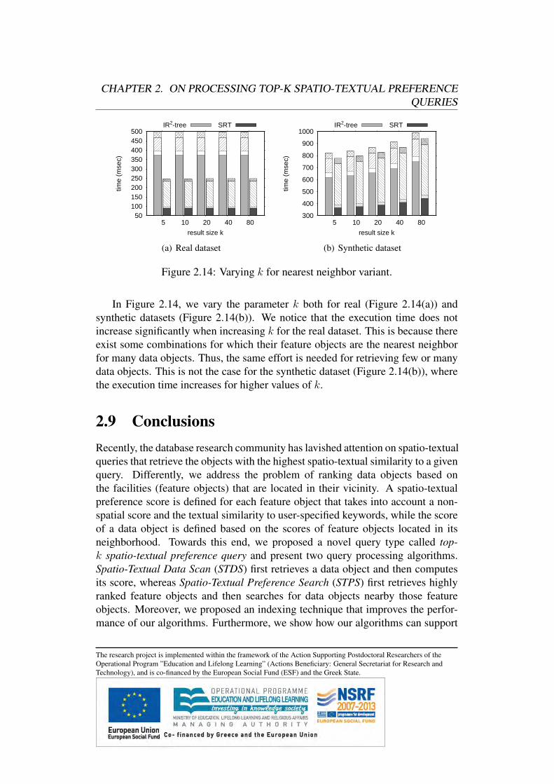
CHAPTER 2. ON PROCESSING TOP-K SPATIO-TEXTUAL PREFERENCEQUERIES
50 100 150 200 250 300 350 400 450 500
5 10 20 40 80
time
(mse
c)
result size k
IR2-tree SRT
(a) Real dataset
300
400
500
600
700
800
900
1000
5 10 20 40 80
time
(mse
c)
result size k
IR2-tree SRT
(b) Synthetic dataset
Figure 2.14: Varying k for nearest neighbor variant.
In Figure 2.14, we vary the parameter k both for real (Figure 2.14(a)) andsynthetic datasets (Figure 2.14(b)). We notice that the execution time does notincrease significantly when increasing k for the real dataset. This is because thereexist some combinations for which their feature objects are the nearest neighborfor many data objects. Thus, the same effort is needed for retrieving few or manydata objects. This is not the case for the synthetic dataset (Figure 2.14(b)), wherethe execution time increases for higher values of k.
2.9 ConclusionsRecently, the database research community has lavished attention on spatio-textualqueries that retrieve the objects with the highest spatio-textual similarity to a givenquery. Differently, we address the problem of ranking data objects based onthe facilities (feature objects) that are located in their vicinity. A spatio-textualpreference score is defined for each feature object that takes into account a non-spatial score and the textual similarity to user-specified keywords, while the scoreof a data object is defined based on the scores of feature objects located in itsneighborhood. Towards this end, we proposed a novel query type called top-k spatio-textual preference query and present two query processing algorithms.Spatio-Textual Data Scan (STDS) first retrieves a data object and then computesits score, whereas Spatio-Textual Preference Search (STPS) first retrieves highlyranked feature objects and then searches for data objects nearby those featureobjects. Moreover, we proposed an indexing technique that improves the perfor-mance of our algorithms. Furthermore, we show how our algorithms can support
The research project is implemented within the framework of the Action Supporting Postdoctoral Researchers of theOperational Program ”Education and Lifelong Learning” (Actions Beneficiary: General Secretariat for Research andTechnology), and is co-financed by the European Social Fund (ESF) and the Greek State.
CHAPTER 2. ON PROCESSING TOP-K SPATIO-TEXTUAL PREFERENCEQUERIES
different score variants. Finally, in our experimental evaluation, we put all meth-ods under scrutiny to verify the efficiency and the scalability of our method forprocessing top-k spatio-textual preference queries.
2.9.1 AcknowledgmentsThis research work was developed in cooperation with George Tsatsanifos and theresearch results where published at:George Tsatsanifos, Akrivi Vlachou: On Processing Top-k Spatio-Textual Pref-erence Queries, in Proceedings of 18th International Conference on ExtendingDatabase Technology (EDBT), Brussels, Belgium, March 23-27, 2015.
The research project is implemented within the framework of the Action Supporting Postdoctoral Researchers of theOperational Program ”Education and Lifelong Learning” (Actions Beneficiary: General Secretariat for Research andTechnology), and is co-financed by the European Social Fund (ESF) and the Greek State.
Chapter 3
Maximizing Influence OfSpatio-Textual Objects ThroughKeyword Selection
In modern applications, spatial objects are increasingly annotated with textualdescriptions, thus offering the opportunity to users to formulate expressive spatio-textual queries that combine spatial distance with textual relevance. For example,given a database of hotels annotated with features (in the form of keywords) ex-tracted from their web page, tourists can pose queries that retrieve a set of hotelsranked based on some combination of distance and textual similarity to the querykeywords. In this context, a challenging problem is how to select a bounded set ofat most b keywords to describe the facilities of a spatial object, in order to makethe object appear in the top-k results of as many users as possible. We formulatethis problem, called Bests-terms, using concepts related to top-k and reverse top-k queries, and show that it is NP-hard. Hence, we present a baseline algorithmthat provides an approximate solution to the problem. Then, we introduce a novelalgorithm for keyword selection that greatly improves the efficiency of query pro-cessing. By means of a thorough experimental evaluation using real data, wedemonstrate the performance gains attained by our approach.
3.1 IntroductionSpatio-textual search has attracted increased attention recently, due to the numer-ous applications that provide value-added services to the users by combining spa-
The research project is implemented within the framework of the Action Supporting Postdoctoral Researchers of theOperational Program ”Education and Lifelong Learning” (Actions Beneficiary: General Secretariat for Research andTechnology), and is co-financed by the European Social Fund (ESF) and the Greek State.
CHAPTER 3. MAXIMIZING INFLUENCE OF SPATIO-TEXTUALOBJECTS THROUGH KEYWORD SELECTION
tial location with textual relevance. Given a database of geographical points ofinterest that are annotated with textual information (also called spatio-textual ob-jects), the objective of a spatio-textual query is to retrieve a ranked set of top-kspatio-textual objects that are close to the query point and have high textual sim-ilarity to the query keywords. As a notable example, consider hotels that are an-notated with their facilities (e.g., in the form of keywords) and tourists that searchfor hotels close to some location of interest and a set of query keywords indicatingdesired facilities (for example “pool” or “Wi-Fi”).
An interesting problem encountered in real-life applications that rely on spatio-textual retrieval is how to improve the ranking of a spatio-textual object for asmany users as possible. For instance, for a newly established hotel at some lo-cation, the question is how to enrich its textual annotation in order to maximizeits rank for many different users. To address this challenging problem, we cap-italize on reverse top-k queries[50], which retrieve the set of users that have agiven object in their top-k results. We model the problem as a maximization ofthe cardinality of the reverse top-k result set, and we explore the different com-binations of keywords that will increase the query object’s rank for many users,when added to its textual annotation. We call this problem as Best terms, we showthat it is NP-hard, and we present a greedy solution that serves as baseline. Then,we propose a novel algorithm that boosts the performance of query processing,by deliberately selecting keywords that increase the score of the query object formany users simultaneously. Finally, we present the results of our experimentalevaluation that verifies the performance gains of our algorithm.
In summary, our main contributions are outlined below:
• We formulate the novel problem, called Best terms, of increasing the rankof a spatio-textual object for many different users, by enriching its textualdescription.
• We show that the Best terms problem is NP-hard and we provide a baselinesolution.
• We propose an efficient query processing algorithm that significantly out-performs the baseline consistently.
• We provide an experimental evaluation that demonstrates the merits of ourapproach.
The rest of this chapter is structured as follows: Section 3.2 provides anoverview of the related work. Section 3.3 presents the necessary background and
The research project is implemented within the framework of the Action Supporting Postdoctoral Researchers of theOperational Program ”Education and Lifelong Learning” (Actions Beneficiary: General Secretariat for Research andTechnology), and is co-financed by the European Social Fund (ESF) and the Greek State.
CHAPTER 3. MAXIMIZING INFLUENCE OF SPATIO-TEXTUALOBJECTS THROUGH KEYWORD SELECTION
preliminary concepts. Then, in Section 3.4, we formally describe the problemstatement. Section 3.5 presents the baseline algorithm, while Section 3.6 describesour efficient query processing algorithm. Section 4.4 shows the experimental eval-uation, and Section 3.8 concludes the chapter.
3.2 Related WorkIn this section, we provide an overview of the related research literature.
Keyword recommendation. Zhang et al. [56] present a method for recom-mending keywords for advertisements in keyword search results using Wikipedia.They focus mostly in cases where the advertisement (target) consists of short-textweb pages which contain inadequate textual content to describe the advertised en-tity. Based on the fact that a large number of entities are described in Wikipedia,they use Wikipedia articles relevant to the advertised entity in order to recom-mend keywords to connect to the target. Fuxman et al. [19] follow a differentapproach. They suggest keyword queries to advertisers using logs which store thequeries posed by the users and the URLs of the result set that were selected bythe users. Some of the URLs are also connected to a set of concepts. The targetof the authors is to connect the set of concepts to the queries using the MarkovRandom Field model and suggest the most relevant queries for each concept tothe advertisers. Ravi et al. [36] propose variety of methods for automatic gen-eration of bid phrases. Among others they introduce the usage of a translationmodel that extends a predefined mapping between bidding phrased and target webpages. Papadimitriou et al. [35] study the problem of mapping an advertisementin a set of URLs based on keyword queries. In particular they assume that eachadvertisement is mapped to a set of keyword queries and their aim is to map eachadvertisement in a set of URLs which will be representative of the results pro-duced by the attached keyword queries. Choi et al. [12] create a representativesummary of the advertisement based on the context of the advertised material.Their method is making use of co-occurrence and semantic vectors in order toenrich the ad context and create a representative set of terms. Cholette et al. [13]study the problem of finding optimal bids in search based algorithms. Agrawalet al. [2] introduce an approach for recommending bid phrases from a given adlanding page by classifying a set of labels generated by click logs. Their classifierhas logarithmic complexity and can efficiently make predictions on large sets oflabels.
The aim of the aforementioned approaches is to identify potentially relevant
The research project is implemented within the framework of the Action Supporting Postdoctoral Researchers of theOperational Program ”Education and Lifelong Learning” (Actions Beneficiary: General Secretariat for Research andTechnology), and is co-financed by the European Social Fund (ESF) and the Greek State.
CHAPTER 3. MAXIMIZING INFLUENCE OF SPATIO-TEXTUALOBJECTS THROUGH KEYWORD SELECTION
queries to the advertised products and form bid phrases based on the identifiedqueries. Our approach is inherently different because the above techniques tryto predict relevant queries and do not consider the relevance of the advertisedproduct in relation to similar products. In addition they do not consider top-ksearch criteria as the appearance of a product in a search result is decided mainlyon the bidding strategy. On the contrary our aim is to enhance the description ofa spatio-textual object and to increase the number of queries for which the targetproduct appears in the top-k list of the search results. In this effort we take intoconsideration not only the user preferences but also the rest of the spatio-textualobjects which are relevant to those queries.
Spatial Keyword Search. Spatial keyword search has been well studied dur-ing the recent years and several index structures have been introduced for efficientsearch. A detailed evaluation of existing spatio-textual indexes can be found in[11]. Felipe et al. [17] introduced the IR2-tree index which integrates a bitmapsignature on each node of an R-tree describing the textual content of the subtreerooted at the node. Cong et al. [14] introduced the IR-tree and its variants. TheIR-tree is based on the R-tree structure as well. Each node of the tree is also as-sociated with inverted index containing the textual information of the children ofthe node. Rocha et al. [38] proposed the S2I index which uses different strategiesfor frequent and infrequent terms. The spatial distribution of a frequent term isstored in an aggregated R-tree (aR-tree) where each node contains an aggregatedvalue of the impact of the term on the objects contained in the subtree rooted atthe node. Cao et al. [7] introduce the concept of prestige where a spatio-textualobject has a higher prestige if it is collocated with other textually similar objects.They calculate the prestige of a spatio-textual object based on a graph where eachnode corresponds to an object and two nodes are connected if and only if theirtextual similarity and spatial proximity exceed certain thresholds.
Ying Lu et al. [32] and Jiaheng Lu et al. [31] studied the problem of reversespatial and textual k nearest neighbor search, where, given a query point q, theobjective is to locate the set of spatio-textual objects for which q is among the knearest neighbors. The distance between the objects is a linear combination of thetextual and the euclidean distance of the objects. The authors introduce the IUR-tree which is an adaptation of the IR-tree. Each node of the IUR-tree containsthe union and the intersection of the terms contained in the objects in the subtreerooted at the node. Our approach is different as we do not evaluate the similaritybetween elements of a set of spatio-textual objects, but our aim to increase therelevance and therefore the visibility of an object against a set of user preferenceswhich constitutes a different set from that of the spatio-textual objects that our
The research project is implemented within the framework of the Action Supporting Postdoctoral Researchers of theOperational Program ”Education and Lifelong Learning” (Actions Beneficiary: General Secretariat for Research andTechnology), and is co-financed by the European Social Fund (ESF) and the Greek State.
CHAPTER 3. MAXIMIZING INFLUENCE OF SPATIO-TEXTUALOBJECTS THROUGH KEYWORD SELECTION
query object belongs.Wu et al. [51] propose the W-IR-tree which is similar to the IR-tree but it
differs in the way it is constructed. While the IR-tree places the objects in leafnodes based on their distance, the W-IR-tree partitions the objects based primarilyon their textual relevance. The W-IR-tree shows improved performance for batchqueries where objects are considered relevant to the query only if they contain allterms of the query. The W-IR-tree cannot be applied in our case as we consider itpossible for a spatio-textual object to be relevant to the a user preference even if itdoes not contain all terms of the user preference.
3.3 PreliminariesLet D be a set of objects where each object o is represented by a tuple of the formo = 〈o.T, o.L〉 where o.T is a set of keywords describing the features of o and Lis a point in R2 describing the location of o. We denote as A =
⋃o∈D o.T to be
the set of all keywords in D. In the scope of this chapter we call these objectsspatio-textual objects. For a given object o, we consider the size of o to be equalto |o.T |, namely the size of an object is the number of terms it contains.
3.3.1 Top-k spatial keyword queriesLet u be a user preference query on D, where u is represented by the a tupleu = 〈u.T, u.L, α〉, u.T ⊆ A is the text describing the user’s desired features,u.L ∈ R2 denotes the desired location and α ∈ R denotes the importance oflocation over matching the desired features. Given a preference u, we can assigna score to each object using the following equation:
f(o, u) = α× δ(o.L, u.L) + (1− α)× θ(o.T, u.T ) (3.1)
where δ(o.L, u.L) is the spatial distance, and θ(o.T, u.T ) is the textual dis-tance between the object o and the user preference u. Given an integer k, we canreturn the top-k spatio-textual objects according to their score. In the scope of thischapter, we assume that lower scores are better, both spatial and textual distancesare normalized in the interval [0, 1] and f(o, u) = 1.0 if θ(o.T, u.T ) = 1. Thelatter assumption implies that objects that are not textually relevant to the querycannot be considered as a valid result.
The textual relevance we employ is the normalized intersection of terms be-tween the description of a spatio-textual object o.T and a user preference keyword
The research project is implemented within the framework of the Action Supporting Postdoctoral Researchers of theOperational Program ”Education and Lifelong Learning” (Actions Beneficiary: General Secretariat for Research andTechnology), and is co-financed by the European Social Fund (ESF) and the Greek State.
CHAPTER 3. MAXIMIZING INFLUENCE OF SPATIO-TEXTUALOBJECTS THROUGH KEYWORD SELECTION
set u.T , i.e., θ(o.T, u.T ) = 1− |o.T⋂u.T ||u.T |−1. Although in large documents
different textual similarity functions are more appropriate, the intersection is morerepresentative in cases of feature selection. For instance if a user is looking for ahotel with a restaurant and a pool, any hotel offering more features (e.g. restau-rant, pool, bar) than the ones specified by the user should not be less textuallyrelevant than a hotel which offers only the features specified by the user prefer-ence (restaurant, pool).
Definition 1 Top-k query. Given a set D of spatio-textual objects, a set of termsA, a scoring function f , an integer k, and a query u, the result set TOPk(u)of a top-k query is a set of spatio-textual objects such that TOPk(u) ⊆ D,|TOPk(u)| = k and ∀o1, o2 : o1 ∈ TOPk(u), o2 ∈ D − TOPk(u) it holds thato1.T
⋂u.T 6= ∅ and f(o1, u) ≤ f(o2, u).
If an object o belongs to the TOPk(u) set of a user preference u, we say thato is visible to u or that u sees o. For a specific set of objects D and a set of userpreferences U , it is possible to identify for a query object q the set of users whocan see q. This is the reverse procedure of a top-k query and therefore it is calledreverse top-k (RTOPk) query [46].
Definition 2 RTOPk query. Given a set D of spatio-textual objects, a set of userqueries U , a scoring function f , integer k, and a spatio-textual object q, the resultset RTOPk(q) of a reverse top-k query is set such that RTOPk(q) ⊆ U andu ∈ RTOPk(q) if and only if ∃o ∈ TOPk(u) such that f(q, u) ≤ f(o, u).
The cardinality of the RTOPk set of a query-object q is called influence scoreof the object and we denote it as I(q). The influence score indicates the numberof users to whom q is visible.
3.3.2 IR-treeWe employ a state-of-the-art index structure to process spatial keyword queries,namely the IR-tree [14]. The IR-tree is an R-tree where each node is associatedwith an inverted index of the objects contained in the respective sub-tree rooted atthe node. In more detail, each leaf node contains an inverted index of the spatio-textual objects contained in the node. The leaf node is characterized by a spatio-textual pseudo-object which consists of a minimum bounding rectangle (MBR)which encloses all objects of the node and a pseudo-document which consists
The research project is implemented within the framework of the Action Supporting Postdoctoral Researchers of theOperational Program ”Education and Lifelong Learning” (Actions Beneficiary: General Secretariat for Research andTechnology), and is co-financed by the European Social Fund (ESF) and the Greek State.
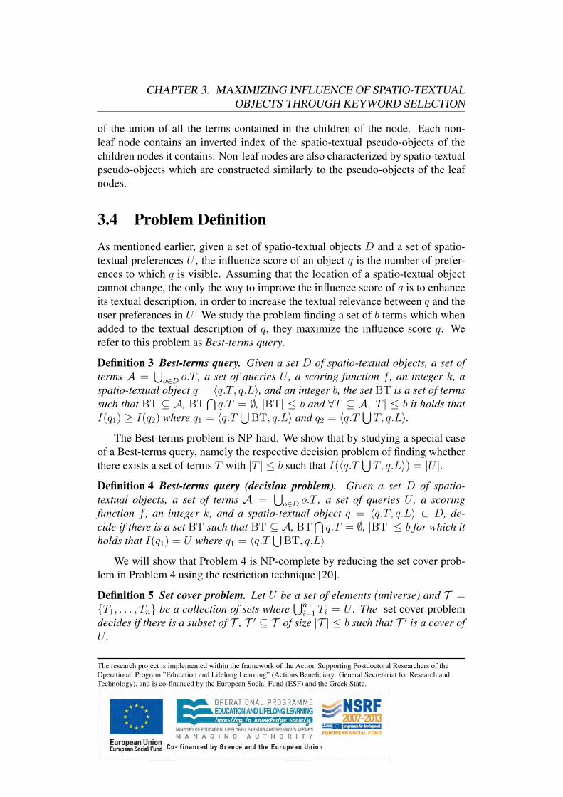
CHAPTER 3. MAXIMIZING INFLUENCE OF SPATIO-TEXTUALOBJECTS THROUGH KEYWORD SELECTION
of the union of all the terms contained in the children of the node. Each non-leaf node contains an inverted index of the spatio-textual pseudo-objects of thechildren nodes it contains. Non-leaf nodes are also characterized by spatio-textualpseudo-objects which are constructed similarly to the pseudo-objects of the leafnodes.
3.4 Problem DefinitionAs mentioned earlier, given a set of spatio-textual objects D and a set of spatio-textual preferences U , the influence score of an object q is the number of prefer-ences to which q is visible. Assuming that the location of a spatio-textual objectcannot change, the only the way to improve the influence score of q is to enhanceits textual description, in order to increase the textual relevance between q and theuser preferences in U . We study the problem finding a set of b terms which whenadded to the textual description of q, they maximize the influence score q. Werefer to this problem as Best-terms query.
Definition 3 Best-terms query. Given a set D of spatio-textual objects, a set ofterms A =
⋃o∈D o.T , a set of queries U , a scoring function f , an integer k, a
spatio-textual object q = 〈q.T, q.L〉, and an integer b, the set BT is a set of termssuch that BT ⊆ A, BT
⋂q.T = ∅, |BT| ≤ b and ∀T ⊆ A, |T | ≤ b it holds that
I(q1) ≥ I(q2) where q1 = 〈q.T⋃
BT, q.L〉 and q2 = 〈q.T⋃T, q.L〉.
The Best-terms problem is NP-hard. We show that by studying a special caseof a Best-terms query, namely the respective decision problem of finding whetherthere exists a set of terms T with |T | ≤ b such that I(〈q.T
⋃T, q.L〉) = |U |.
Definition 4 Best-terms query (decision problem). Given a set D of spatio-textual objects, a set of terms A =
⋃o∈D o.T , a set of queries U , a scoring
function f , an integer k, and a spatio-textual object q = 〈q.T, q.L〉 ∈ D, de-cide if there is a set BT such that BT ⊆ A, BT
⋂q.T = ∅, |BT| ≤ b for which it
holds that I(q1) = U where q1 = 〈q.T⋃
BT, q.L〉
We will show that Problem 4 is NP-complete by reducing the set cover prob-lem in Problem 4 using the restriction technique [20].
Definition 5 Set cover problem. Let U be a set of elements (universe) and T ={T1, . . . , Tn} be a collection of sets where
⋃ni=1 Ti = U . The set cover problem
decides if there is a subset of T , T ′ ⊆ T of size |T | ≤ b such that T ′ is a cover ofU .
The research project is implemented within the framework of the Action Supporting Postdoctoral Researchers of theOperational Program ”Education and Lifelong Learning” (Actions Beneficiary: General Secretariat for Research andTechnology), and is co-financed by the European Social Fund (ESF) and the Greek State.
CHAPTER 3. MAXIMIZING INFLUENCE OF SPATIO-TEXTUALOBJECTS THROUGH KEYWORD SELECTION
Proof. Let an oracle machine select the BT set for a query object q. We setp = 〈q.T
⋃BT, q.L〉 and by performing a TOPk query for each user preference
we can calculate the RTOPk(p) set and the influence score I(p) of object p inpolynomial time. Therefore the solution can be verified in polynomial time andour problem belongs to the NP class.
We set U a to be a set of users and D = {q}. We define a collection T ={T1, . . . , T|A|} of sets, one for each term ti in A where a user u belongs in Tionly if ti ∈ u.T . If we consider k = 1, then, for all users that q.T
⋂u.T = ∅
it holds that q 6∈ TOPk(u) since q is not relevant to u.T . If q.T⋂u.T 6= ∅ then
q ∈ TOPk(u) as it is the only object. Therefore any selection of a term ti isequivalent of selecting a subset of Ti of U . The set cover problem can thereforebe seen as a special case of Problem 4 and therefore Problem 4 is NP-completewhich leads us to the conclusion that the Best-terms problem is NP-hard.
3.5 BaselineIn this section we describe a baseline approximate solution for the Best-termsproblem. An exact solution is infeasible to be calculated as the the problem isNP-hard. Therefore we use a greedy algorithm, HRJN (Best Term First), whichon each step adds to the query object the term that induces the highest increase ininfluence score.
Algorithm 6 describes the HRJN approach. HRJN takes as input an IR-treeindex containing the set of spatio-textual objects D, and an IR-tree index con-taining the set of user preferences U . It starts by creating a pseudo-preferenceq′, in order to traverse the preferences based on their distance to the query objectq. It first creates a set C of candidate spatio-textual objects, one for each termthat can be added to q. The size of C is equal to |A − q.T |. In lines 10,11 thealgorithm checks if performing a top-k query is necessary. It calculates the scoreof the last retrieved spatio-textual objects with the scores of the candidate objectsand if there are k objects which have a better score than all objects in C, the userpreference is ignored as no candidate object can be in the TOPk set of the currentuser preference. In the opposite case the top-k query is executed and the TOPk
result set is stored in the buffer. All candidate objects which are no worse thanthe k-best element of the calculated TOPk set belong also to the TOPk set of uand therefore their influence score is increased. When all user preferences havebeen examined, the object with the highest influence score is selected and a new
The research project is implemented within the framework of the Action Supporting Postdoctoral Researchers of theOperational Program ”Education and Lifelong Learning” (Actions Beneficiary: General Secretariat for Research andTechnology), and is co-financed by the European Social Fund (ESF) and the Greek State.

CHAPTER 3. MAXIMIZING INFLUENCE OF SPATIO-TEXTUALOBJECTS THROUGH KEYWORD SELECTION
Algorithm 6 HRJNInput: U :set of users,D: set of objects,
q:query point, b : number of new termsOutput: BT: set of new terms
1: C ← ∅,2: q′ ← 〈q.T, q.L, 1〉3: bestCandidate← q4: for i = 0; i < b; i+ + do //repeat until b new terms have been found5: for all t ∈ A− o.T do6: C ← C
⋃{〈bestCandidate.T
⋃{t}, bestCandidate.L〉}
7: end for8: u←next(U,q′)9: while u 6= null do
10: τ ← maxp∈buffer
(f(p, u))
11: if ∃c ∈ C : f(c, u) ≤ τ then12: buffer← TOPk(u)13: τ ← max
p∈buffer(f(p, u))
14: for all c ∈ C do15: if f(c, u) ≤ τ then16: I(c)← I(c) + 117: end if18: end for19: u←next(U,q′)20: end if21: end while22: bestCandidate← argmax
c(I(c))
23: end for24: BT← bestCandidate.T-q.T25: return BT
The research project is implemented within the framework of the Action Supporting Postdoctoral Researchers of theOperational Program ”Education and Lifelong Learning” (Actions Beneficiary: General Secretariat for Research andTechnology), and is co-financed by the European Social Fund (ESF) and the Greek State.
CHAPTER 3. MAXIMIZING INFLUENCE OF SPATIO-TEXTUALOBJECTS THROUGH KEYWORD SELECTION
set of candidate objects is created based on that object. The procedure is repeatedb times until an object with b new terms is created. The terms that are included inthe resulting object and not in q constitute the resulting BT set.
The IR-tree index on U helps us reduce the number TOPk queries executed.As the preferences are accessed by ascending distance, the score of q is expectedto reduce and therefore it becomes less likely for a TOPk query to be executed.
3.6 Graph Based Term SelectionHRJN extends the textual description of a spatio-textual object incrementally, factthat forces the algorithm to scan the preferences multiple times leading to a highcomputational cost. In the section we present a new algorithm GBTS (GraphBased Term Selection) which examines the set of preferences only once per queryobject and creates a graph of terms which provides an estimation of the influencegain any combination of terms may provide.
GBTS consists of two separate algorithms. The first algorithm GC (GraphConstruction) creates a graph connecting the terms which when added to a spatio-textual object q, they can induce an increase in its influence score. The secondalgorithm BSS (Best Subgraph Selection) traverses the graph identifying the setsof terms which will induce the highest increase in the influence score of q. In moredetail, given a set of objects D, a set of user preferences U and a spatio-textualobject q, we denote as U(q) the set of all preferences for which q is not visibleand at most b terms are needed for q to become visible. The first algorithm, GC,constructs a weighted graph G = (V,E) where each node of the graph representsa candidate term, and the edges connecting the nodes indicate the maximum in-crease in the influence score of q if a set of terms is added to q. For each examineduser preference u, the algorithm adds to the graph a node for each previously un-seen term. If one additional term is enough for u to be added to RTOPk(q), thealgorithm adds a loop edge with weight equal to 1, to each term t that is not con-tained in q. If the edge already exists, the weight is simply added to the existingedge. In cases where more than one terms are necessary for q to be included toTOPk(u), the procedure is slightly different. Let T = u.T − q.T = {t1, . . . , tn}be the terms that are included in u but not in q and 1 < λ ≤ n, be the num-ber of terms that need to be added to u for it to be included in the RTOPk(q).For each pair of terms in u.T − q.T , the algorithm adds an edge with weightequal to 2 (λ(λ− 1))−1. The sum of weights of the edges added to each subgraphG′ = (V ′, E ′) where V ′ ⊆ T and |V ′| = λ is equal to 1 indicating the potential
The research project is implemented within the framework of the Action Supporting Postdoctoral Researchers of theOperational Program ”Education and Lifelong Learning” (Actions Beneficiary: General Secretariat for Research andTechnology), and is co-financed by the European Social Fund (ESF) and the Greek State.

CHAPTER 3. MAXIMIZING INFLUENCE OF SPATIO-TEXTUALOBJECTS THROUGH KEYWORD SELECTION
Algorithm 7 GCInput: U :set of users,D: set of objects,
q:query point, b : number of new termsOutput: G = (V,E): resulting graph
1: V = ∅, E = ∅, G = (V,E) //graph initialization2: q′ ← 〈q.T, q.L, 1〉3: u← next(U, q′)4: while u 6= null do5: buffer← TOPk(u)6: τ ← max
p∈buffer(f(p, u))
7: if f(q, u) > τ then //if q 6∈ TOPk(u)
8: T ← u.T − q.T9: V ← V
⋃T
10: λ← max
(1,
⌈(1− τ − aδ(q, u)
1− a
)|u|⌉)
11: if λ ≤ 1 then12: E ← E
⋃{e = (ti, ti, 1) : ti ∈ T}
13: else if 1 < λ ≤ b then
14: E ← E⋃{
e =
(ti, tj,
2
λ(λ− 1)
): ti, tj ∈ T and ti 6= tj
}15: end if16: end if17: u←next(U,q′)18: end while19: return G
increase in the influence score of q if the terms contained in G′ are added to q. Asbefore, if an edge already exists, the weight is added to the existing edge.
When the graph has been created, algorithm BSS (Best Subgraph Selection)chooses as seed nodes the b nodes (terms) of the graph with the highest degreeand creates a set of b subgraphs with initially one node each. Next, each subgraphis expanded by adding at each step the node with highest degree that is adjacent tothe subgraph. The expansion of each subgraph is continued until each subgraphhas b nodes or the subgraph cannot be expanded. Finally the subgraph with thehighest sum of edges is selected as solution and the set of terms included in thesubgraph are the ones that constitute the BT set.
Algorithm 7 describes the construction of the term graph G. GC starts with
The research project is implemented within the framework of the Action Supporting Postdoctoral Researchers of theOperational Program ”Education and Lifelong Learning” (Actions Beneficiary: General Secretariat for Research andTechnology), and is co-financed by the European Social Fund (ESF) and the Greek State.
CHAPTER 3. MAXIMIZING INFLUENCE OF SPATIO-TEXTUALOBJECTS THROUGH KEYWORD SELECTION
Algorithm 8 BSSInput: G = (V,E): graph, b: number of desired termsOutput: BT:set of new terms
1: Q← ∅ //Priority Queue2: BT← ∅3: for i = 0; i < b; i+ + do4: ti ← next node of G with the highest degree5: Gti ← expandNode(ti)6: Q.add(sumOfWeights(Gti),Gti)7: end for8: while |BT| ≤ b do9: GS ←Q.pop()
10: add to BT the b− |BT| highest degree nodes from GS
11: end while12: return BT
creating a pseudo-preference in order to traverse the preferences based on theirdistance to q. For each user preference if q is not in the TOPk(u) set, GC updatesthe node set of G and calculates λ, the number of terms that need to be addedin q for it to be included in the TOPk(u) set. The number of terms is calculatedbased Equation 3.1 and the minimum score q is required to have in order to be inthe TOPk(u) set. A non-positive value of λ indicates that u is located near q butq.T
⋂u.T = ∅ and therefore q is not included in the TOPk(u) set. The addition
of any term will allow q to be added to TOPk(u) set and therefore one loop edgeis added to each term t for which it holds t ∈ u.T − q.T . If more than one termsare necessary to be added in q (λ > 1), GC adds all necessary edges in the graph.The algorithm continues until all user preferences have been examined. The sizeof the graph depends on the number of distinct terms contained in U(q). Theterms correspond to the features extracted from the textual descriptions of spatio-textual objects that describe the offered facilities. In practice, we have noticed thatthe vocabulary for the targeted applications is limited and therefore the graph isexpected to fit in the main memory.
Algorithm 8 describes the algorithm of term selection. Initially an empty pri-ority queue (Q) is constructed. Subsequently, at line 4 the algorithm chooses asseed the highest degree node ti that has not yet been selected and constructs thesubgraph Gti (line 5). The subgraph is constructed by repeatedly selecting thehighest degree node adjacent to the Gti until |Gti| = b or until no nodes can be
The research project is implemented within the framework of the Action Supporting Postdoctoral Researchers of theOperational Program ”Education and Lifelong Learning” (Actions Beneficiary: General Secretariat for Research andTechnology), and is co-financed by the European Social Fund (ESF) and the Greek State.
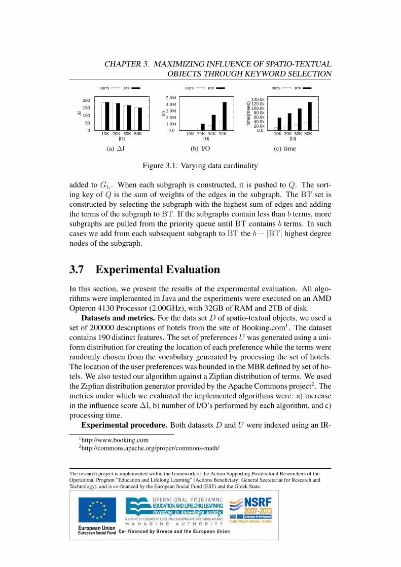
CHAPTER 3. MAXIMIZING INFLUENCE OF SPATIO-TEXTUALOBJECTS THROUGH KEYWORD SELECTION
0
50
100
150
200
10K 20K 30K 50K
∆I
|D|
GBTS BTF
(a) ∆I
0.0
1.0M
2.0M
3.0M
4.0M
5.0M
10K 20K 30K 50K
IO
|D|
GBTS BTF
(b) I/O
0.0 20.0k 40.0k 60.0k 80.0k
100.0k 120.0k 140.0k
10K 20K 30K 50K
tim
e(m
sec)
|D|
GBTS BTF
(c) time
Figure 3.1: Varying data cardinality
added to Gti . When each subgraph is constructed, it is pushed to Q. The sort-ing key of Q is the sum of weights of the edges in the subgraph. The BT set isconstructed by selecting the subgraph with the highest sum of edges and addingthe terms of the subgraph to BT. If the subgraphs contain less than b terms, moresubgraphs are pulled from the priority queue until BT contains b terms. In suchcases we add from each subsequent subgraph to BT the b − |BT| highest degreenodes of the subgraph.
3.7 Experimental EvaluationIn this section, we present the results of the experimental evaluation. All algo-rithms were implemented in Java and the experiments were executed on an AMDOpteron 4130 Processor (2.00GHz), with 32GB of RAM and 2TB of disk.
Datasets and metrics. For the data set D of spatio-textual objects, we used aset of 200000 descriptions of hotels from the site of Booking.com1. The datasetcontains 190 distinct features. The set of preferences U was generated using a uni-form distribution for creating the location of each preference while the terms wererandomly chosen from the vocabulary generated by processing the set of hotels.The location of the user preferences was bounded in the MBR defined by set of ho-tels. We also tested our algorithm against a Zipfian distribution of terms. We usedthe Zipfian distribution generator provided by the Apache Commons project2. Themetrics under which we evaluated the implemented algorithms were: a) increasein the influence score ∆I, b) number of I/O’s performed by each algorithm, and c)processing time.
Experimental procedure. Both datasets D and U were indexed using an IR-
1http://www.booking.com2http://commons.apache.org/proper/commons-math/
The research project is implemented within the framework of the Action Supporting Postdoctoral Researchers of theOperational Program ”Education and Lifelong Learning” (Actions Beneficiary: General Secretariat for Research andTechnology), and is co-financed by the European Social Fund (ESF) and the Greek State.
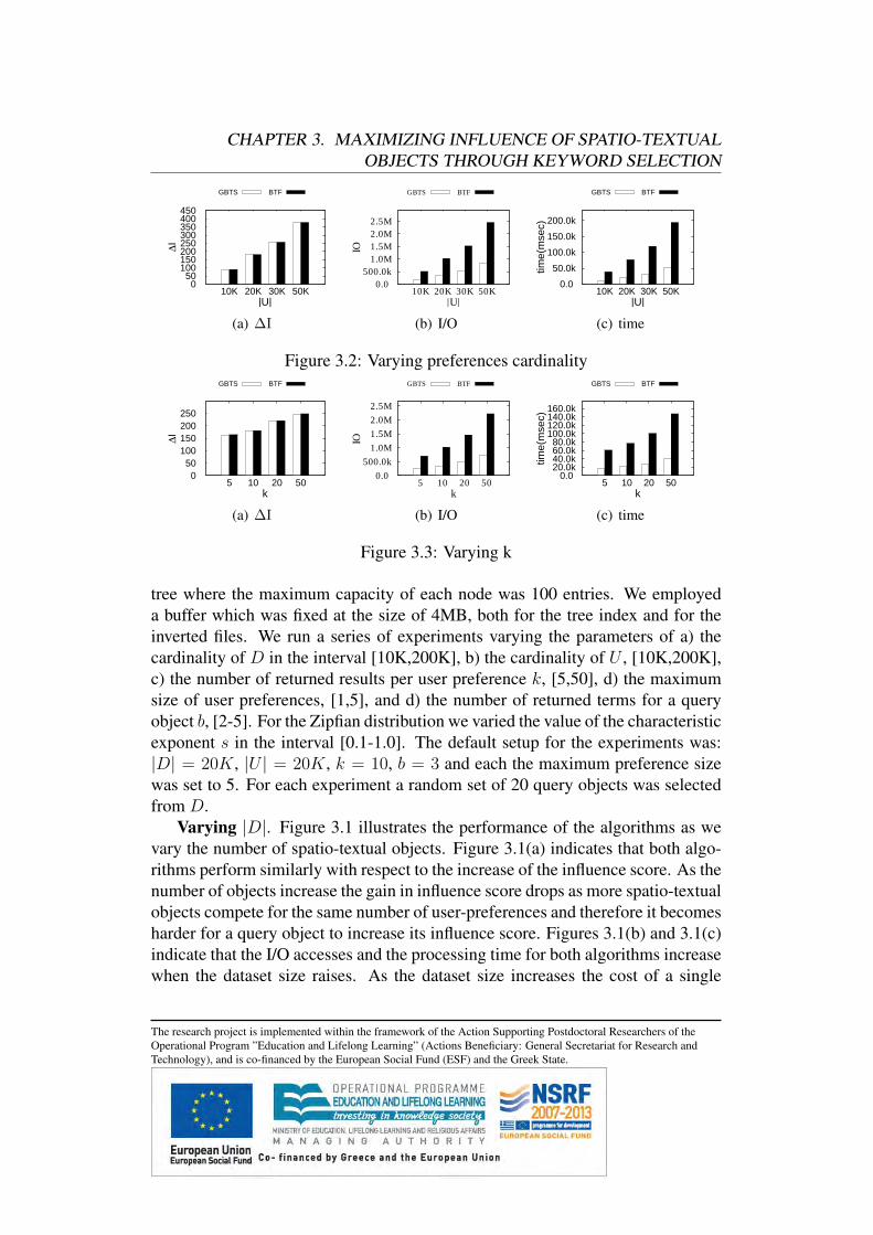
CHAPTER 3. MAXIMIZING INFLUENCE OF SPATIO-TEXTUALOBJECTS THROUGH KEYWORD SELECTION
0 50 100 150 200 250 300 350 400 450
10K 20K 30K 50K
∆I
|U|
GBTS BTF
(a) ∆I
0.0
500.0k
1.0M
1.5M
2.0M
2.5M
10K 20K 30K 50K
IO
|U|
GBTS BTF
(b) I/O
0.0
50.0k
100.0k
150.0k
200.0k
10K 20K 30K 50K
tim
e(m
sec)
|U|
GBTS BTF
(c) time
Figure 3.2: Varying preferences cardinality
0
50
100
150
200
250
5 10 20 50
∆I
k
GBTS BTF
(a) ∆I
0.0
500.0k
1.0M
1.5M
2.0M
2.5M
5 10 20 50
IO
k
GBTS BTF
(b) I/O
0.0 20.0k 40.0k 60.0k 80.0k
100.0k 120.0k 140.0k 160.0k
5 10 20 50
tim
e(m
sec)
k
GBTS BTF
(c) time
Figure 3.3: Varying k
tree where the maximum capacity of each node was 100 entries. We employeda buffer which was fixed at the size of 4MB, both for the tree index and for theinverted files. We run a series of experiments varying the parameters of a) thecardinality of D in the interval [10K,200K], b) the cardinality of U , [10K,200K],c) the number of returned results per user preference k, [5,50], d) the maximumsize of user preferences, [1,5], and d) the number of returned terms for a queryobject b, [2-5]. For the Zipfian distribution we varied the value of the characteristicexponent s in the interval [0.1-1.0]. The default setup for the experiments was:|D| = 20K, |U | = 20K, k = 10, b = 3 and each the maximum preference sizewas set to 5. For each experiment a random set of 20 query objects was selectedfrom D.
Varying |D|. Figure 3.1 illustrates the performance of the algorithms as wevary the number of spatio-textual objects. Figure 3.1(a) indicates that both algo-rithms perform similarly with respect to the increase of the influence score. As thenumber of objects increase the gain in influence score drops as more spatio-textualobjects compete for the same number of user-preferences and therefore it becomesharder for a query object to increase its influence score. Figures 3.1(b) and 3.1(c)indicate that the I/O accesses and the processing time for both algorithms increasewhen the dataset size raises. As the dataset size increases the cost of a single
The research project is implemented within the framework of the Action Supporting Postdoctoral Researchers of theOperational Program ”Education and Lifelong Learning” (Actions Beneficiary: General Secretariat for Research andTechnology), and is co-financed by the European Social Fund (ESF) and the Greek State.
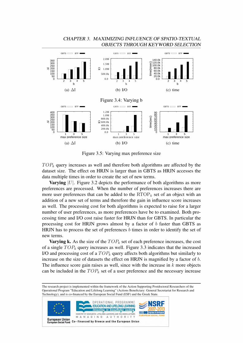
CHAPTER 3. MAXIMIZING INFLUENCE OF SPATIO-TEXTUALOBJECTS THROUGH KEYWORD SELECTION
0 50 100 150 200 250 300 350
2 3 4 5
∆I
b
GBTS BTF
(a) ∆I
0.0
500.0k
1.0M
1.5M
2.0M
2 3 4 5
IO
b
GBTS BTF
(b) I/O
0.0 20.0k 40.0k 60.0k 80.0k
100.0k 120.0k 140.0k
2 3 4 5
tim
e(m
sec)
b
GBTS BTF
(c) time
Figure 3.4: Varying b
0 50 100 150 200 250 300 350 400
1 3 5
∆I
max preference size
GBTS BTF
(a) ∆I
0.0
200.0k
400.0k
600.0k
800.0k
1.0M
1.2M
1 3 5
IO
max preference size
GBTS BTF
(b) I/O
0 10 20 30 40 50 60 70 80 90
1 3 5
tim
e(s
ec)
max preference size
GBTS BTF
(c) time
Figure 3.5: Varying max preference size
TOPk query increases as well and therefore both algorithms are affected by thedataset size. The effect on HRJN is larger than in GBTS as HRJN accesses thedata multiple times in order to create the set of new terms.
Varying |U |. Figure 3.2 depicts the performance of both algorithms as morepreferences are processed. When the number of preferences increases there aremore user preferences that can be added to the RTOPk set of an object with anaddition of a new set of terms and therefore the gain in influence score increasesas well. The processing cost for both algorithms is expected to raise for a largernumber of user preferences, as more preferences have be to examined. Both pro-cessing time and I/O cost raise faster for HRJN than for GBTS. In particular theprocessing cost for HRJN grows almost by a factor of b faster than GBTS asHRJN has to process the set of preferences b times in order to identify the set ofnew terms.
Varying k. As the size of the TOPk set of each preference increases, the costof a single TOPk query increases as well. Figure 3.3 indicates that the increasedI/O and processing cost of a TOPk query affects both algorithms but similarly toincrease on the size of datasets the effect on HRJN is magnified by a factor of b.The influence score gain raises as well, since with the increase in k more objectscan be included in the TOPk set of a user preference and the necessary increase
The research project is implemented within the framework of the Action Supporting Postdoctoral Researchers of theOperational Program ”Education and Lifelong Learning” (Actions Beneficiary: General Secretariat for Research andTechnology), and is co-financed by the European Social Fund (ESF) and the Greek State.
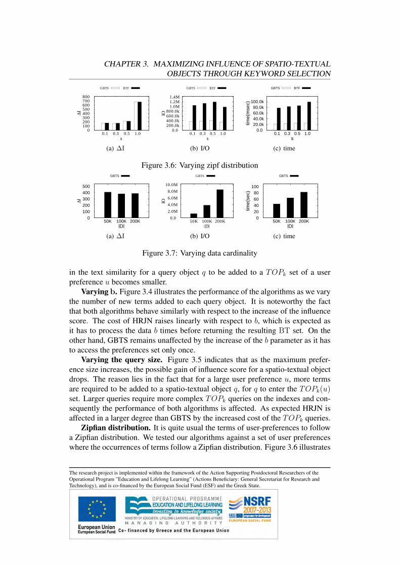
CHAPTER 3. MAXIMIZING INFLUENCE OF SPATIO-TEXTUALOBJECTS THROUGH KEYWORD SELECTION
0 100 200 300 400 500 600 700 800
0.1 0.3 0.5 1.0
∆I
s
GBTS BTF
(a) ∆I
0.0 200.0k 400.0k 600.0k 800.0k
1.0M 1.2M 1.4M
0.1 0.3 0.5 1.0
IO
s
GBTS BTF
(b) I/O
0.0
20.0k
40.0k
60.0k
80.0k
100.0k
0.1 0.3 0.5 1.0
tim
e(m
sec)
s
GBTS BTF
(c) time
Figure 3.6: Varying zipf distribution
0
100
200
300
400
500
50K 100K 200K
∆I
|D|
GBTS
(a) ∆I
0.0
2.0M
4.0M
6.0M
8.0M
10.0M
50K 100K 200K
IO
|D|
GBTS
(b) I/O
0
20
40
60
80
100
50K 100K 200K
tim
e(s
ec)
|D|
GBTS
(c) time
Figure 3.7: Varying data cardinality
in the text similarity for a query object q to be added to a TOPk set of a userpreference u becomes smaller.
Varying b. Figure 3.4 illustrates the performance of the algorithms as we varythe number of new terms added to each query object. It is noteworthy the factthat both algorithms behave similarly with respect to the increase of the influencescore. The cost of HRJN raises linearly with respect to b, which is expected asit has to process the data b times before returning the resulting BT set. On theother hand, GBTS remains unaffected by the increase of the b parameter as it hasto access the preferences set only once.
Varying the query size. Figure 3.5 indicates that as the maximum prefer-ence size increases, the possible gain of influence score for a spatio-textual objectdrops. The reason lies in the fact that for a large user preference u, more termsare required to be added to a spatio-textual object q, for q to enter the TOPk(u)set. Larger queries require more complex TOPk queries on the indexes and con-sequently the performance of both algorithms is affected. As expected HRJN isaffected in a larger degree than GBTS by the increased cost of the TOPk queries.
Zipfian distribution. It is quite usual the terms of user-preferences to followa Zipfian distribution. We tested our algorithms against a set of user preferenceswhere the occurrences of terms follow a Zipfian distribution. Figure 3.6 illustrates
The research project is implemented within the framework of the Action Supporting Postdoctoral Researchers of theOperational Program ”Education and Lifelong Learning” (Actions Beneficiary: General Secretariat for Research andTechnology), and is co-financed by the European Social Fund (ESF) and the Greek State.
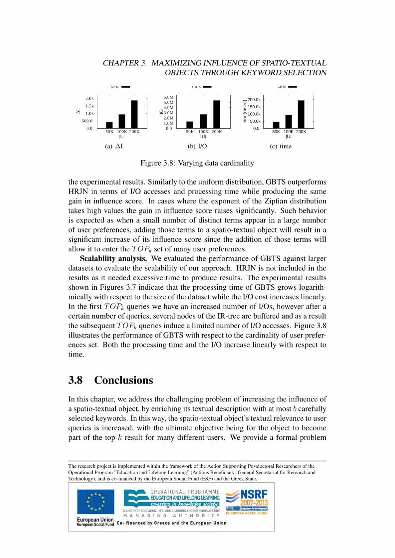
CHAPTER 3. MAXIMIZING INFLUENCE OF SPATIO-TEXTUALOBJECTS THROUGH KEYWORD SELECTION
0.0
500.0
1.0k
1.5k
2.0k
50K 100K 200K
∆I
|U|
GBTS
(a) ∆I
0.0
1.0M
2.0M
3.0M
4.0M
5.0M
6.0M
50K 100K 200K
IO
|U|
GBTS
(b) I/O
0.0
50.0k
100.0k
150.0k
200.0k
50K 100K 200K
tim
e(m
sec)
|U|
GBTS
(c) time
Figure 3.8: Varying data cardinality
the experimental results. Similarly to the uniform distribution, GBTS outperformsHRJN in terms of I/O accesses and processing time while producing the samegain in influence score. In cases where the exponent of the Zipfian distributiontakes high values the gain in influence score raises significantly. Such behavioris expected as when a small number of distinct terms appear in a large numberof user preferences, adding those terms to a spatio-textual object will result in asignificant increase of its influence score since the addition of those terms willallow it to enter the TOPk set of many user preferences.
Scalability analysis. We evaluated the performance of GBTS against largerdatasets to evaluate the scalability of our approach. HRJN is not included in theresults as it needed excessive time to produce results. The experimental resultsshown in Figures 3.7 indicate that the processing time of GBTS grows logarith-mically with respect to the size of the dataset while the I/O cost increases linearly.In the first TOPk queries we have an increased number of I/Os, however after acertain number of queries, several nodes of the IR-tree are buffered and as a resultthe subsequent TOPk queries induce a limited number of I/O accesses. Figure 3.8illustrates the performance of GBTS with respect to the cardinality of user prefer-ences set. Both the processing time and the I/O increase linearly with respect totime.
3.8 ConclusionsIn this chapter, we address the challenging problem of increasing the influence ofa spatio-textual object, by enriching its textual description with at most b carefullyselected keywords. In this way, the spatio-textual object’s textual relevance to userqueries is increased, with the ultimate objective being for the object to becomepart of the top-k result for many different users. We provide a formal problem
The research project is implemented within the framework of the Action Supporting Postdoctoral Researchers of theOperational Program ”Education and Lifelong Learning” (Actions Beneficiary: General Secretariat for Research andTechnology), and is co-financed by the European Social Fund (ESF) and the Greek State.

CHAPTER 3. MAXIMIZING INFLUENCE OF SPATIO-TEXTUALOBJECTS THROUGH KEYWORD SELECTION
statement that is novel and relies on concepts related to top-k and reverse top-kqueries. We show that the problem is NP-hard, and we present a greedy solutionto the problem. Then, we propose a more efficient algorithm that achieves resultsof comparable quality, but with significantly lower processing cost. We demon-strate the performance gains of the proposed approach by means of a thoroughexperimental evaluation that includes real data.
3.8.1 AcknowledgmentsThis research work was developed in cooperation with Orestis Gkorgkas, ChristosDoulkeridis and Kjetil Nørvag and the research results are under submission:Orestis Gkorgkas, Akrivi Vlachou, Christos Doulkeridis, Kjetil Nørvag: Maxi-mizing Influence of Spatio-Textual Objects through Keyword Selection submittedfor publication.
The research project is implemented within the framework of the Action Supporting Postdoctoral Researchers of theOperational Program ”Education and Lifelong Learning” (Actions Beneficiary: General Secretariat for Research andTechnology), and is co-financed by the European Social Fund (ESF) and the Greek State.
Chapter 4
Location-aware TagRecommendations for Flickr
Flickr is one of the largest online image collections, where shared photos are typ-ically annotated with tags. The tagging process bridges the gap between visualcontent and keyword search by providing a meaningful textual description of thetagged object. However, the task of tagging is cumbersome, therefore tag recom-mendation is commonly used to suggest relevant tags to the user and enrich thesemantic description of the photo. Apart from textual tagging based on keywords,an increasing trend of geotagging has been recently observed, as witnessed by theincreased number of geotagged photos in Flickr. Geotagging refers to attachinglocation-specific information to photos, namely about the location where a photowas captured. Even though there exist different methods for tag recommendationof photos, the gain of using spatial and textual information in order to recom-mend more meaningful tags to users has not been studied yet. We analyze theproperties of geotagged photos of Flickr, and propose novel location-aware tagrecommendation methods. For evaluation purposes, we have implemented a pro-totype system and exploit it to present examples that demonstrate the effectivenessof our proposed methods.
4.1 IntroductionFlickr allows users to upload photos, annotate the photos with tags,view photosuploaded by other users, comment on photos, create special interest groups etc.Currently, Flickr stores one of the largest online image collections with more than
The research project is implemented within the framework of the Action Supporting Postdoctoral Researchers of theOperational Program ”Education and Lifelong Learning” (Actions Beneficiary: General Secretariat for Research andTechnology), and is co-financed by the European Social Fund (ESF) and the Greek State.
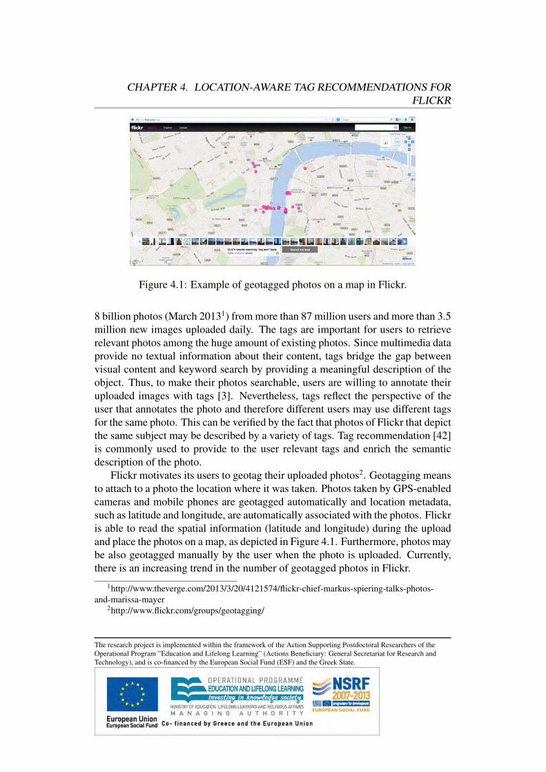
CHAPTER 4. LOCATION-AWARE TAG RECOMMENDATIONS FORFLICKR
Figure 4.1: Example of geotagged photos on a map in Flickr.
8 billion photos (March 20131) from more than 87 million users and more than 3.5million new images uploaded daily. The tags are important for users to retrieverelevant photos among the huge amount of existing photos. Since multimedia dataprovide no textual information about their content, tags bridge the gap betweenvisual content and keyword search by providing a meaningful description of theobject. Thus, to make their photos searchable, users are willing to annotate theiruploaded images with tags [3]. Nevertheless, tags reflect the perspective of theuser that annotates the photo and therefore different users may use different tagsfor the same photo. This can be verified by the fact that photos of Flickr that depictthe same subject may be described by a variety of tags. Tag recommendation [42]is commonly used to provide to the user relevant tags and enrich the semanticdescription of the photo.
Flickr motivates its users to geotag their uploaded photos2. Geotagging meansto attach to a photo the location where it was taken. Photos taken by GPS-enabledcameras and mobile phones are geotagged automatically and location metadata,such as latitude and longitude, are automatically associated with the photos. Flickris able to read the spatial information (latitude and longitude) during the uploadand place the photos on a map, as depicted in Figure 4.1. Furthermore, photos maybe also geotagged manually by the user when the photo is uploaded. Currently,there is an increasing trend in the number of geotagged photos in Flickr.
1http://www.theverge.com/2013/3/20/4121574/flickr-chief-markus-spiering-talks-photos-and-marissa-mayer
2http://www.flickr.com/groups/geotagging/
The research project is implemented within the framework of the Action Supporting Postdoctoral Researchers of theOperational Program ”Education and Lifelong Learning” (Actions Beneficiary: General Secretariat for Research andTechnology), and is co-financed by the European Social Fund (ESF) and the Greek State.
CHAPTER 4. LOCATION-AWARE TAG RECOMMENDATIONS FORFLICKR
Even though several recent studies [14, 6] examine how relevant web objectscan be retrieved based on both the spatial and textual information, the gain ofusing spatial information in order to recommend more meaningful tags to usershas not been studied yet. Nevertheless, it is expected that nearby photos maydepict similar objects, thus sharing common tags with higher probability. In thischapter, we propose methods for tag recommendations based on both locationand tag co-occurrence of the photos. In details, this work makes the followingcontributions:
• We create different data collections of geo-tagged photos of Flickr that arelocated in different cities and analyze their properties in terms of tag fre-quency, number of tags per photos and the type of tags commonly chosenby users. This study allows us to analyze the behavior of the users related totagging and draw some important conclusions for our tag recommendationmethods.
• We introduce novel tag recommendation methods that take into account alsothe location of the given photo as well as the location of the existing pho-tos. The key idea of our methods is that not only the similarity in terms ofexisting tags is important, but also the distance between the existing photosin which the tags appear.
• We implemented a prototype system for location-aware tag recommenda-tions over photos of Flickr and evaluate experimentally our proposed methodthrough examples that demonstrates the effectiveness of location-aware tagrecommendation.
The remainder of the chapter is structured as follows. In Section 4.2 we de-scribe our data collections and analyze their properties. Then, Section 4.3 presentsan overview of the location-aware tag recommendations system and describes theproposed location-aware tag recommendation methods. In Section 4.4 we evalu-ate our proposed methods. Finally, in Section 4.5 we discuss related work and inSection 4.6 we provide some concluding remarks.
4.2 Data CollectionIn this section we describe our data collections and provide statistics about thephoto tags. In order to design our recommendation strategies it is important to first
The research project is implemented within the framework of the Action Supporting Postdoctoral Researchers of theOperational Program ”Education and Lifelong Learning” (Actions Beneficiary: General Secretariat for Research andTechnology), and is co-financed by the European Social Fund (ESF) and the Greek State.
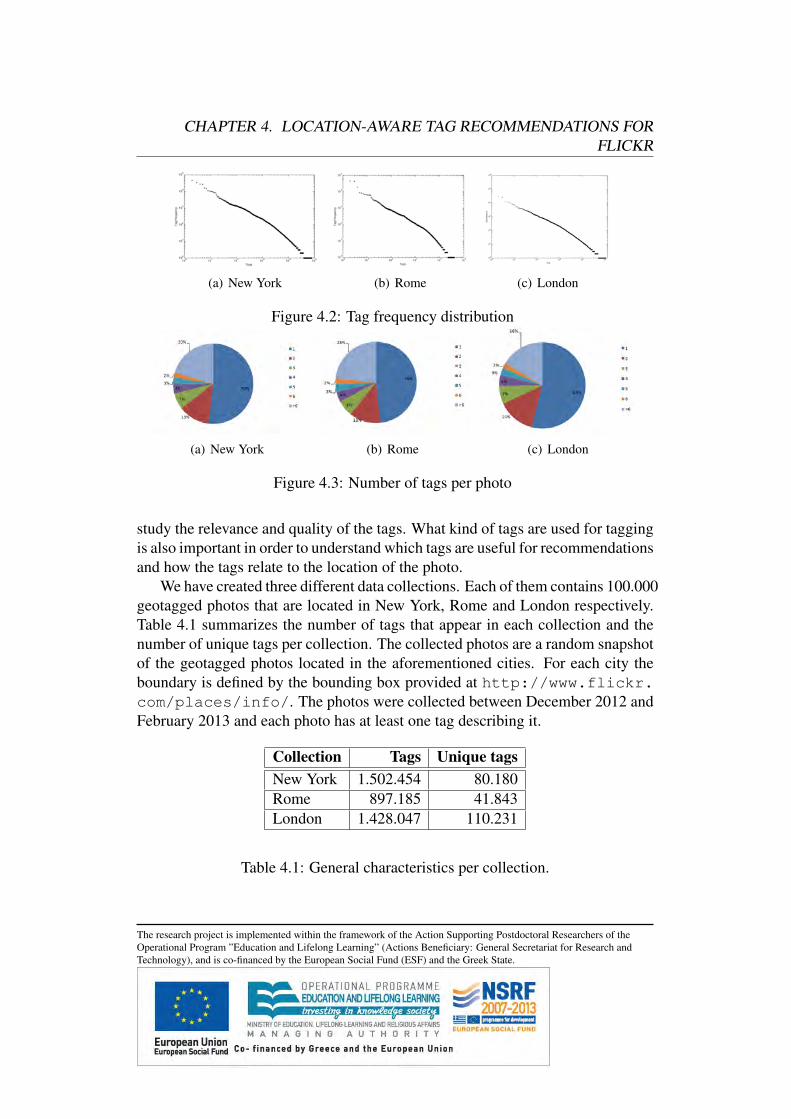
CHAPTER 4. LOCATION-AWARE TAG RECOMMENDATIONS FORFLICKR
(a) New York (b) Rome (c) London
Figure 4.2: Tag frequency distribution
(a) New York (b) Rome (c) London
Figure 4.3: Number of tags per photo
study the relevance and quality of the tags. What kind of tags are used for taggingis also important in order to understand which tags are useful for recommendationsand how the tags relate to the location of the photo.
We have created three different data collections. Each of them contains 100.000geotagged photos that are located in New York, Rome and London respectively.Table 4.1 summarizes the number of tags that appear in each collection and thenumber of unique tags per collection. The collected photos are a random snapshotof the geotagged photos located in the aforementioned cities. For each city theboundary is defined by the bounding box provided at http://www.flickr.com/places/info/. The photos were collected between December 2012 andFebruary 2013 and each photo has at least one tag describing it.
Collection Tags Unique tagsNew York 1.502.454 80.180Rome 897.185 41.843London 1.428.047 110.231
Table 4.1: General characteristics per collection.
The research project is implemented within the framework of the Action Supporting Postdoctoral Researchers of theOperational Program ”Education and Lifelong Learning” (Actions Beneficiary: General Secretariat for Research andTechnology), and is co-financed by the European Social Fund (ESF) and the Greek State.
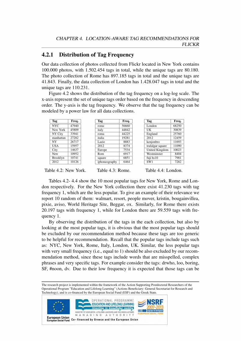
CHAPTER 4. LOCATION-AWARE TAG RECOMMENDATIONS FORFLICKR
4.2.1 Distribution of Tag FrequencyOur data collection of photos collected from Flickr located in New York contains100.000 photos, with 1.502.454 tags in total, while the unique tags are 80.180.The photo collection of Rome has 897.185 tags in total and the unique tags are41.843. Finally, the data collection of London has 1.428.047 tags in total and theunique tags are 110.231.
Figure 4.2 shows the distribution of the tag frequency on a log-log scale. Thex-axis represent the set of unique tags order based on the frequency in descendingorder. The y-axis is the tag frequency. We observe that the tag frequency can bemodeled by a power law for all data collections.
Tag Freq.NYC 47940New York 45809NY City 33941manhattan 27282NY 26717USA 15957City 14637New 10952Brooklyn 107412012 10126
Table 4.2: New York.
Tag Freq.rome 56660italy 44842roma 44225italia 19281Lazio 88832012 8374Europe 7534Rom 6917square 6851iphoneography 6464
Table 4.3: Rome.
Tag Freq.London 68250UK 30839England 257602012 12459kenjonbro 11693trafalgar square 11090United Kingdom 10023Westminster 8404fuji hs10 7981SW1 7282
Table 4.4: London.
Tables 4.2- 4.4 show the 10 most popular tags for New York, Rome and Lon-don respectively. For the New York collection there exist 41.230 tags with tagfrequency 1, which are the less popular. To give an example of their relevance wereport 10 random of them: walmart, resort, people mover, kristin, bougainvillea,pixie, aviso, World Heritage Site, Beggar, ox. Similarly, for Rome there exists20.197 tags with frequency 1, while for London there are 59.559 tags with fre-quency 1.
By observing the distribution of the tags in the each collection, but also bylooking at the most popular tags, it is obvious that the most popular tags shouldbe excluded by our recommendation method because these tags are too genericto be helpful for recommendation. Recall that the popular tags include tags suchas: NYC, New York, Rome, Italy, London, UK. Similar, the less popular tagswith very small frequency (i.e., equal to 1) should be also excluded by our recom-mendation method, since these tags include words that are misspelled, complexphrases and very specific tags. For example consider the tags: drwho, loo, boring,SF, #noon, dv. Due to their low frequency it is expected that those tags can be
The research project is implemented within the framework of the Action Supporting Postdoctoral Researchers of theOperational Program ”Education and Lifelong Learning” (Actions Beneficiary: General Secretariat for Research andTechnology), and is co-financed by the European Social Fund (ESF) and the Greek State.
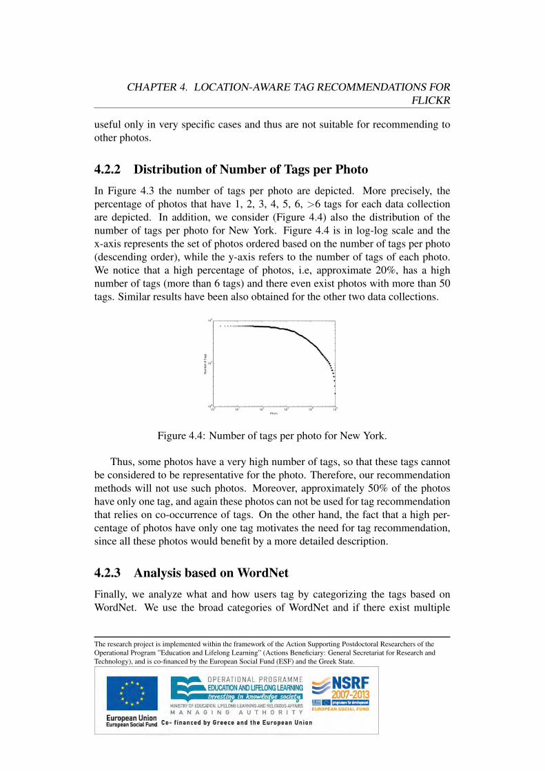
CHAPTER 4. LOCATION-AWARE TAG RECOMMENDATIONS FORFLICKR
useful only in very specific cases and thus are not suitable for recommending toother photos.
4.2.2 Distribution of Number of Tags per PhotoIn Figure 4.3 the number of tags per photo are depicted. More precisely, thepercentage of photos that have 1, 2, 3, 4, 5, 6, >6 tags for each data collectionare depicted. In addition, we consider (Figure 4.4) also the distribution of thenumber of tags per photo for New York. Figure 4.4 is in log-log scale and thex-axis represents the set of photos ordered based on the number of tags per photo(descending order), while the y-axis refers to the number of tags of each photo.We notice that a high percentage of photos, i.e, approximate 20%, has a highnumber of tags (more than 6 tags) and there even exist photos with more than 50tags. Similar results have been also obtained for the other two data collections.
Figure 4.4: Number of tags per photo for New York.
Thus, some photos have a very high number of tags, so that these tags cannotbe considered to be representative for the photo. Therefore, our recommendationmethods will not use such photos. Moreover, approximately 50% of the photoshave only one tag, and again these photos can not be used for tag recommendationthat relies on co-occurrence of tags. On the other hand, the fact that a high per-centage of photos have only one tag motivates the need for tag recommendation,since all these photos would benefit by a more detailed description.
4.2.3 Analysis based on WordNetFinally, we analyze what and how users tag by categorizing the tags based onWordNet. We use the broad categories of WordNet and if there exist multiple
The research project is implemented within the framework of the Action Supporting Postdoctoral Researchers of theOperational Program ”Education and Lifelong Learning” (Actions Beneficiary: General Secretariat for Research andTechnology), and is co-financed by the European Social Fund (ESF) and the Greek State.
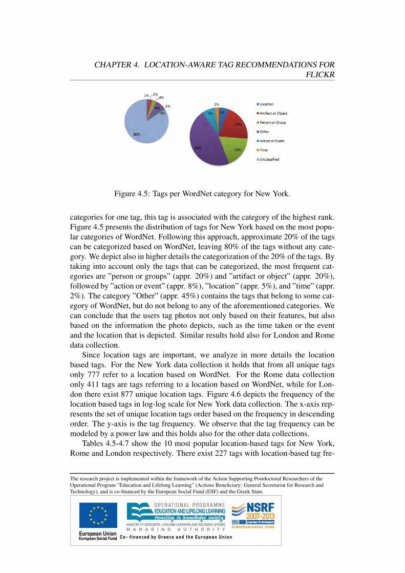
CHAPTER 4. LOCATION-AWARE TAG RECOMMENDATIONS FORFLICKR
Figure 4.5: Tags per WordNet category for New York.
categories for one tag, this tag is associated with the category of the highest rank.Figure 4.5 presents the distribution of tags for New York based on the most popu-lar categories of WordNet. Following this approach, approximate 20% of the tagscan be categorized based on WordNet, leaving 80% of the tags without any cate-gory. We depict also in higher details the categorization of the 20% of the tags. Bytaking into account only the tags that can be categorized, the most frequent cat-egories are ”person or groups” (appr. 20%) and ”artifact or object” (appr. 20%),followed by ”action or event” (appr. 8%), ”location” (appr. 5%), and ”time” (appr.2%). The category ”Other” (appr. 45%) contains the tags that belong to some cat-egory of WordNet, but do not belong to any of the aforementioned categories. Wecan conclude that the users tag photos not only based on their features, but alsobased on the information the photo depicts, such as the time taken or the eventand the location that is depicted. Similar results hold also for London and Romedata collection.
Since location tags are important, we analyze in more details the locationbased tags. For the New York data collection it holds that from all unique tagsonly 777 refer to a location based on WordNet. For the Rome data collectiononly 411 tags are tags referring to a location based on WordNet, while for Lon-don there exist 877 unique location tags. Figure 4.6 depicts the frequency of thelocation based tags in log-log scale for New York data collection. The x-axis rep-resents the set of unique location tags order based on the frequency in descendingorder. The y-axis is the tag frequency. We observe that the tag frequency can bemodeled by a power law and this holds also for the other data collections.
Tables 4.5-4.7 show the 10 most popular location-based tags for New York,Rome and London respectively. There exist 227 tags with location-based tag fre-
The research project is implemented within the framework of the Action Supporting Postdoctoral Researchers of theOperational Program ”Education and Lifelong Learning” (Actions Beneficiary: General Secretariat for Research andTechnology), and is co-financed by the European Social Fund (ESF) and the Greek State.
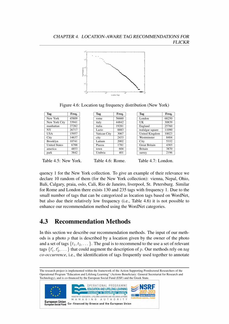
CHAPTER 4. LOCATION-AWARE TAG RECOMMENDATIONS FORFLICKR
Figure 4.6: Location tag frequency distribution (New York)
Tag Freq.New York 45809New York City 33941manhattan 27282NY 26717USA 15957City 14637Brooklyn 10741United States 6788america 4853park 3842
Table 4.5: New York.
Tag Freq.rome 56660italy 44842italia 19281Lazio 8883Vatican City 3067city 2433Latium 2002Piazza 1781town 604Umbria 401
Table 4.6: Rome.
Tag Freq.London 68250UK 30839England 25760trafalgar square 11090United Kingdom 10023Westminster 8404City 5332Great Britain 4303Britain 3870surrey 2196
Table 4.7: London.
quency 1 for the New York collection. To give an example of their relevance wedeclare 10 random of them (for the New York collection): vienna, Nepal, Ohio,Bali, Calgary, praia, oslo, Cali, Rio de Janeiro, liverpool, St. Petersburg. Similarfor Rome and London there exists 130 and 235 tags with frequency 1. Due to thesmall number of tags that can be categorized as location tags based on WordNet,but also due their relatively low frequency (i.e., Table 4.6) it is not possible toenhance our recommendation method using the WordNet categories.
4.3 Recommendation MethodsIn this section we describe our recommendation methods. The input of our meth-ods is a photo p that is described by a location given by the owner of the photoand a set of tags {t1, t2, . . . }. The goal is to recommend to the use a set of relevanttags {t′1, t′2, . . . } that could augment the description of p. Our methods rely on tagco-occurrence, i.e., the identification of tags frequently used together to annotate
The research project is implemented within the framework of the Action Supporting Postdoctoral Researchers of theOperational Program ”Education and Lifelong Learning” (Actions Beneficiary: General Secretariat for Research andTechnology), and is co-financed by the European Social Fund (ESF) and the Greek State.
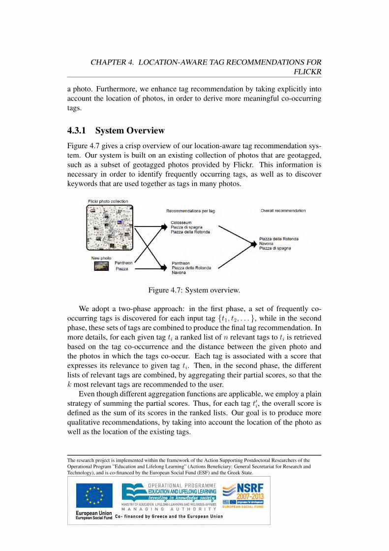
CHAPTER 4. LOCATION-AWARE TAG RECOMMENDATIONS FORFLICKR
a photo. Furthermore, we enhance tag recommendation by taking explicitly intoaccount the location of photos, in order to derive more meaningful co-occurringtags.
4.3.1 System OverviewFigure 4.7 gives a crisp overview of our location-aware tag recommendation sys-tem. Our system is built on an existing collection of photos that are geotagged,such as a subset of geotagged photos provided by Flickr. This information isnecessary in order to identify frequently occurring tags, as well as to discoverkeywords that are used together as tags in many photos.
Figure 4.7: System overview.
We adopt a two-phase approach: in the first phase, a set of frequently co-occurring tags is discovered for each input tag {t1, t2, . . . }, while in the secondphase, these sets of tags are combined to produce the final tag recommendation. Inmore details, for each given tag ti a ranked list of n relevant tags to ti is retrievedbased on the tag co-occurrence and the distance between the given photo andthe photos in which the tags co-occur. Each tag is associated with a score thatexpresses its relevance to given tag ti. Then, in the second phase, the differentlists of relevant tags are combined, by aggregating their partial scores, so that thek most relevant tags are recommended to the user.
Even though different aggregation functions are applicable, we employ a plainstrategy of summing the partial scores. Thus, for each tag t′i, the overall score isdefined as the sum of its scores in the ranked lists. Our goal is to produce morequalitative recommendations, by taking into account the location of the photo aswell as the location of the existing tags.
The research project is implemented within the framework of the Action Supporting Postdoctoral Researchers of theOperational Program ”Education and Lifelong Learning” (Actions Beneficiary: General Secretariat for Research andTechnology), and is co-financed by the European Social Fund (ESF) and the Greek State.
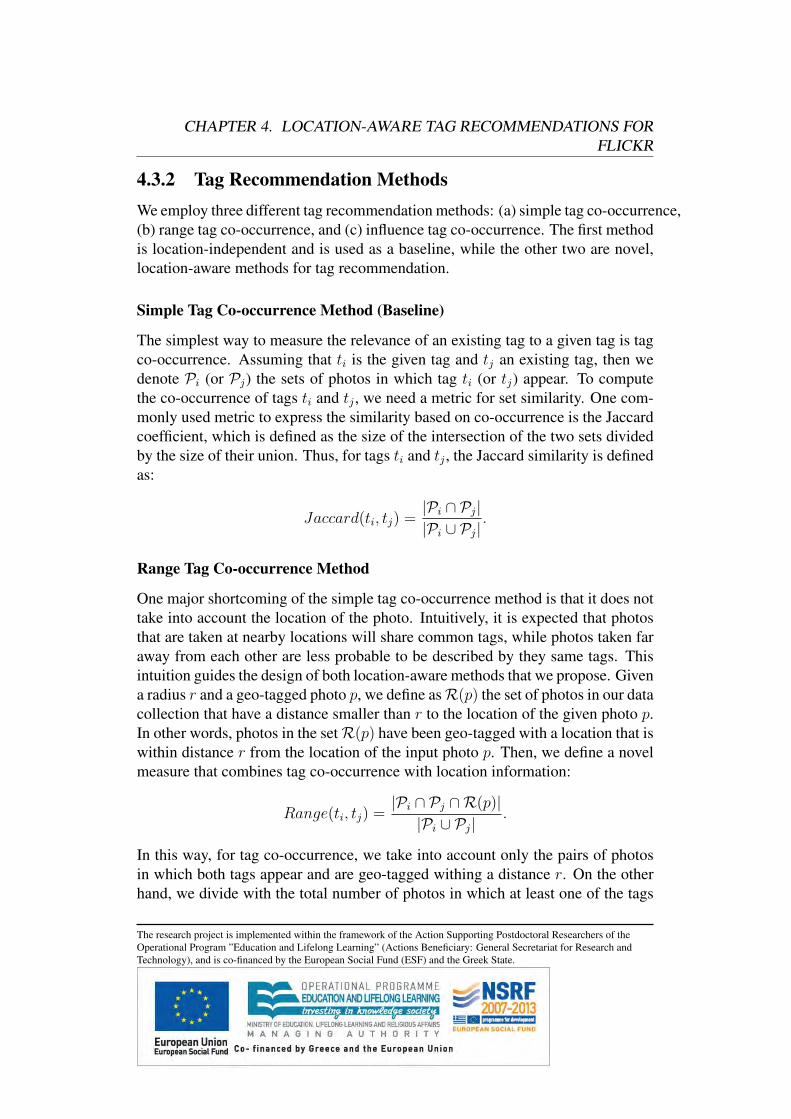
CHAPTER 4. LOCATION-AWARE TAG RECOMMENDATIONS FORFLICKR
4.3.2 Tag Recommendation MethodsWe employ three different tag recommendation methods: (a) simple tag co-occurrence,(b) range tag co-occurrence, and (c) influence tag co-occurrence. The first methodis location-independent and is used as a baseline, while the other two are novel,location-aware methods for tag recommendation.
Simple Tag Co-occurrence Method (Baseline)
The simplest way to measure the relevance of an existing tag to a given tag is tagco-occurrence. Assuming that ti is the given tag and tj an existing tag, then wedenote Pi (or Pj) the sets of photos in which tag ti (or tj) appear. To computethe co-occurrence of tags ti and tj , we need a metric for set similarity. One com-monly used metric to express the similarity based on co-occurrence is the Jaccardcoefficient, which is defined as the size of the intersection of the two sets dividedby the size of their union. Thus, for tags ti and tj , the Jaccard similarity is definedas:
Jaccard(ti, tj) =|Pi ∩ Pj||Pi ∪ Pj|
.
Range Tag Co-occurrence Method
One major shortcoming of the simple tag co-occurrence method is that it does nottake into account the location of the photo. Intuitively, it is expected that photosthat are taken at nearby locations will share common tags, while photos taken faraway from each other are less probable to be described by they same tags. Thisintuition guides the design of both location-aware methods that we propose. Givena radius r and a geo-tagged photo p, we define asR(p) the set of photos in our datacollection that have a distance smaller than r to the location of the given photo p.In other words, photos in the setR(p) have been geo-tagged with a location that iswithin distance r from the location of the input photo p. Then, we define a novelmeasure that combines tag co-occurrence with location information:
Range(ti, tj) =|Pi ∩ Pj ∩R(p)||Pi ∪ Pj|
.
In this way, for tag co-occurrence, we take into account only the pairs of photosin which both tags appear and are geo-tagged withing a distance r. On the otherhand, we divide with the total number of photos in which at least one of the tags
The research project is implemented within the framework of the Action Supporting Postdoctoral Researchers of theOperational Program ”Education and Lifelong Learning” (Actions Beneficiary: General Secretariat for Research andTechnology), and is co-financed by the European Social Fund (ESF) and the Greek State.
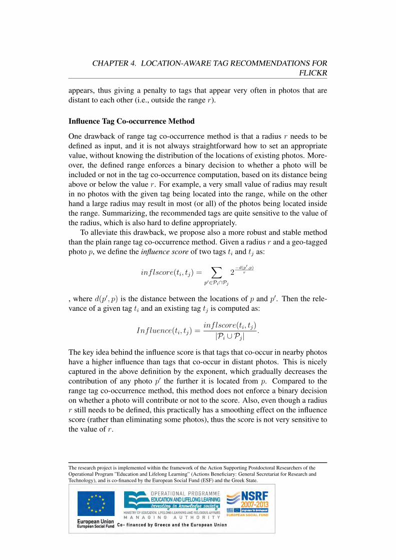
CHAPTER 4. LOCATION-AWARE TAG RECOMMENDATIONS FORFLICKR
appears, thus giving a penalty to tags that appear very often in photos that aredistant to each other (i.e., outside the range r).
Influence Tag Co-occurrence Method
One drawback of range tag co-occurrence method is that a radius r needs to bedefined as input, and it is not always straightforward how to set an appropriatevalue, without knowing the distribution of the locations of existing photos. More-over, the defined range enforces a binary decision to whether a photo will beincluded or not in the tag co-occurrence computation, based on its distance beingabove or below the value r. For example, a very small value of radius may resultin no photos with the given tag being located into the range, while on the otherhand a large radius may result in most (or all) of the photos being located insidethe range. Summarizing, the recommended tags are quite sensitive to the value ofthe radius, which is also hard to define appropriately.
To alleviate this drawback, we propose also a more robust and stable methodthan the plain range tag co-occurrence method. Given a radius r and a geo-taggedphoto p, we define the influence score of two tags ti and tj as:
inflscore(ti, tj) =∑
p′∈Pi∩Pj
2−d(p′,p)
r
, where d(p′, p) is the distance between the locations of p and p′. Then the rele-vance of a given tag ti and an existing tag tj is computed as:
Influence(ti, tj) =inflscore(ti, tj)
|Pi ∪ Pj|.
The key idea behind the influence score is that tags that co-occur in nearby photoshave a higher influence than tags that co-occur in distant photos. This is nicelycaptured in the above definition by the exponent, which gradually decreases thecontribution of any photo p′ the further it is located from p. Compared to therange tag co-occurrence method, this method does not enforce a binary decisionon whether a photo will contribute or not to the score. Also, even though a radiusr still needs to be defined, this practically has a smoothing effect on the influencescore (rather than eliminating some photos), thus the score is not very sensitive tothe value of r.
The research project is implemented within the framework of the Action Supporting Postdoctoral Researchers of theOperational Program ”Education and Lifelong Learning” (Actions Beneficiary: General Secretariat for Research andTechnology), and is co-financed by the European Social Fund (ESF) and the Greek State.
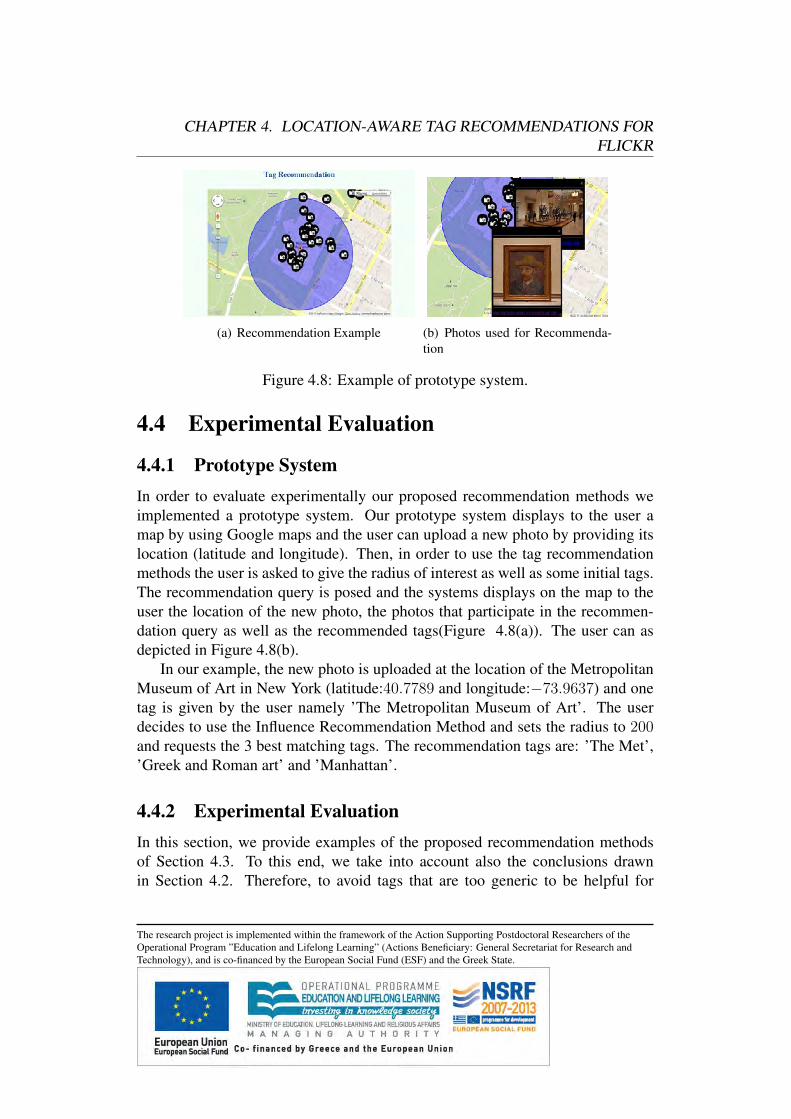
CHAPTER 4. LOCATION-AWARE TAG RECOMMENDATIONS FORFLICKR
(a) Recommendation Example (b) Photos used for Recommenda-tion
Figure 4.8: Example of prototype system.
4.4 Experimental Evaluation
4.4.1 Prototype SystemIn order to evaluate experimentally our proposed recommendation methods weimplemented a prototype system. Our prototype system displays to the user amap by using Google maps and the user can upload a new photo by providing itslocation (latitude and longitude). Then, in order to use the tag recommendationmethods the user is asked to give the radius of interest as well as some initial tags.The recommendation query is posed and the systems displays on the map to theuser the location of the new photo, the photos that participate in the recommen-dation query as well as the recommended tags(Figure 4.8(a)). The user can asdepicted in Figure 4.8(b).
In our example, the new photo is uploaded at the location of the MetropolitanMuseum of Art in New York (latitude:40.7789 and longitude:−73.9637) and onetag is given by the user namely ’The Metropolitan Museum of Art’. The userdecides to use the Influence Recommendation Method and sets the radius to 200and requests the 3 best matching tags. The recommendation tags are: ’The Met’,’Greek and Roman art’ and ’Manhattan’.
4.4.2 Experimental EvaluationIn this section, we provide examples of the proposed recommendation methodsof Section 4.3. To this end, we take into account also the conclusions drawnin Section 4.2. Therefore, to avoid tags that are too generic to be helpful for
The research project is implemented within the framework of the Action Supporting Postdoctoral Researchers of theOperational Program ”Education and Lifelong Learning” (Actions Beneficiary: General Secretariat for Research andTechnology), and is co-financed by the European Social Fund (ESF) and the Greek State.
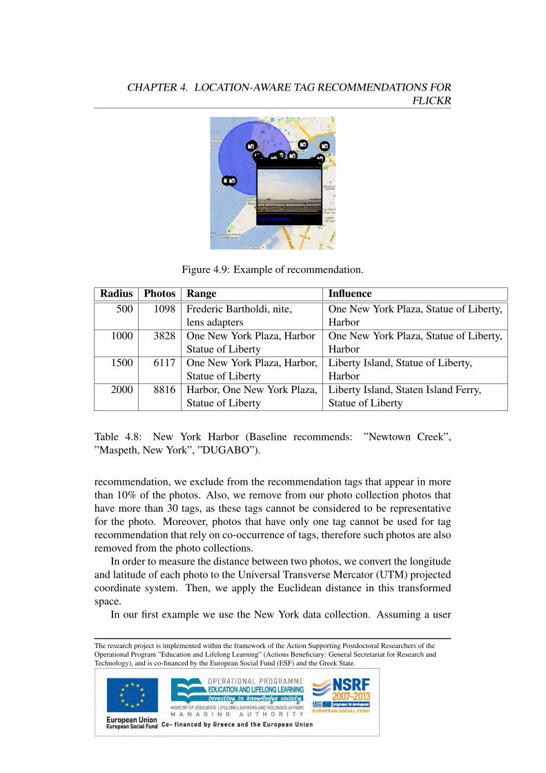
CHAPTER 4. LOCATION-AWARE TAG RECOMMENDATIONS FORFLICKR
Figure 4.9: Example of recommendation.
Radius Photos Range Influence500 1098 Frederic Bartholdi, nite, One New York Plaza, Statue of Liberty,
lens adapters Harbor1000 3828 One New York Plaza, Harbor One New York Plaza, Statue of Liberty,
Statue of Liberty Harbor1500 6117 One New York Plaza, Harbor, Liberty Island, Statue of Liberty,
Statue of Liberty Harbor2000 8816 Harbor, One New York Plaza, Liberty Island, Staten Island Ferry,
Statue of Liberty Statue of Liberty
Table 4.8: New York Harbor (Baseline recommends: ”Newtown Creek”,”Maspeth, New York”, ”DUGABO”).
recommendation, we exclude from the recommendation tags that appear in morethan 10% of the photos. Also, we remove from our photo collection photos thathave more than 30 tags, as these tags cannot be considered to be representativefor the photo. Moreover, photos that have only one tag cannot be used for tagrecommendation that rely on co-occurrence of tags, therefore such photos are alsoremoved from the photo collections.
In order to measure the distance between two photos, we convert the longitudeand latitude of each photo to the Universal Transverse Mercator (UTM) projectedcoordinate system. Then, we apply the Euclidean distance in this transformedspace.
In our first example we use the New York data collection. Assuming a user
The research project is implemented within the framework of the Action Supporting Postdoctoral Researchers of theOperational Program ”Education and Lifelong Learning” (Actions Beneficiary: General Secretariat for Research andTechnology), and is co-financed by the European Social Fund (ESF) and the Greek State.
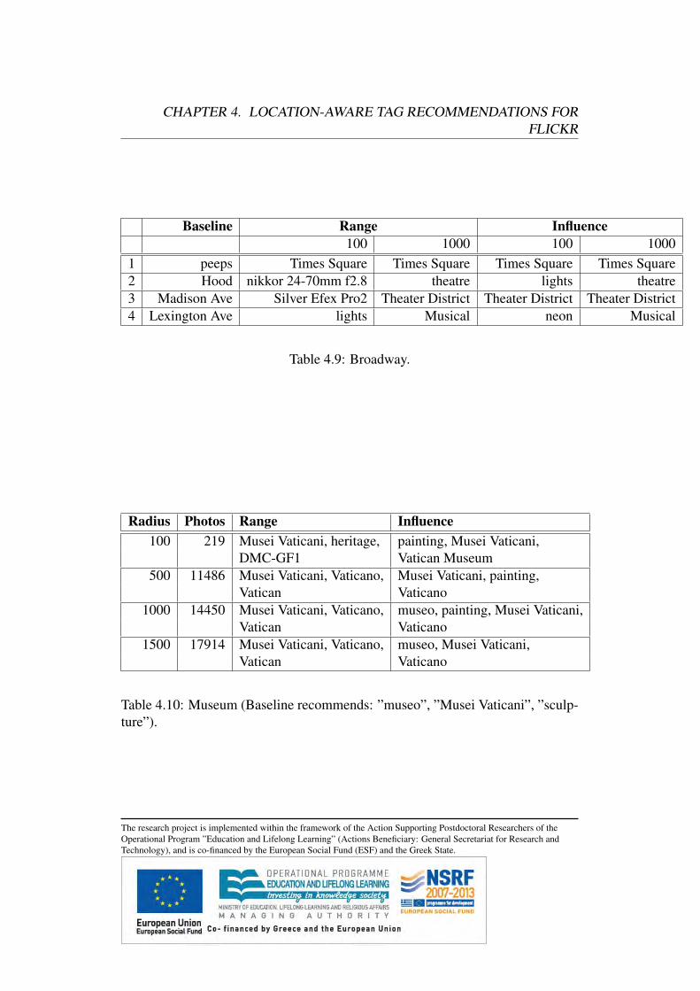
CHAPTER 4. LOCATION-AWARE TAG RECOMMENDATIONS FORFLICKR
Baseline Range Influence100 1000 100 1000
1 peeps Times Square Times Square Times Square Times Square2 Hood nikkor 24-70mm f2.8 theatre lights theatre3 Madison Ave Silver Efex Pro2 Theater District Theater District Theater District4 Lexington Ave lights Musical neon Musical
Table 4.9: Broadway.
Radius Photos Range Influence100 219 Musei Vaticani, heritage, painting, Musei Vaticani,
DMC-GF1 Vatican Museum500 11486 Musei Vaticani, Vaticano, Musei Vaticani, painting,
Vatican Vaticano1000 14450 Musei Vaticani, Vaticano, museo, painting, Musei Vaticani,
Vatican Vaticano1500 17914 Musei Vaticani, Vaticano, museo, Musei Vaticani,
Vatican Vaticano
Table 4.10: Museum (Baseline recommends: ”museo”, ”Musei Vaticani”, ”sculp-ture”).
The research project is implemented within the framework of the Action Supporting Postdoctoral Researchers of theOperational Program ”Education and Lifelong Learning” (Actions Beneficiary: General Secretariat for Research andTechnology), and is co-financed by the European Social Fund (ESF) and the Greek State.
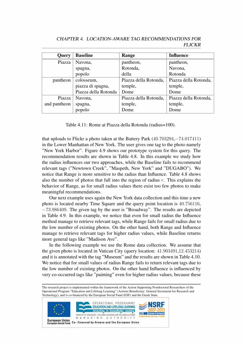
CHAPTER 4. LOCATION-AWARE TAG RECOMMENDATIONS FORFLICKR
Query Baseline Range InfluencePiazza Navona, pantheon, pantheon,
spagna, Rotonda, Navona,popolo della Rotonda
pantheon colosseum, Piazza della Rotonda, Piazza della Rotonda,piazza di spagna, temple, temple,Piazza della Rotonda Dome Dome
Piazza Navona, Piazza della Rotonda, Piazza della Rotonda,and pantheon spagna, temple, temple,
popolo Dome Dome
Table 4.11: Rome at Piazza della Rotonda (radius=100).
that uploads to Flickr a photo taken at the Battery Park (40.703294,−74.017411)in the Lower Manhattan of New York. The user gives one tag to the photo namely”New York Harbor”. Figure 4.9 shows our prototype system for this query. Therecommendation results are shown in Table 4.8. In this example we study howthe radius influences our two approaches, while the Baseline fails to recommendrelevant tags (”Newtown Creek”, ”Maspeth, New York” and ”DUGABO”). Wenotice that Range is more sensitive to the radius than Influence. Table 4.8 showsalso the number of photos that fall into the region of radius r. This explains thebehavior of Range, as for small radius values there exist too few photos to makemeaningful recommendations.
Our next example uses again the New York data collection and this time a newphoto is located nearby Time Square and the query point location is 40.756116,−73.986409. The given tag by the user is ”Broadway”. The results are depictedin Table 4.9. In this example, we notice that even for small radius the Influencemethod manage to retrieve relevant tags, while Range fails for small radius due tothe low number of existing photos. On the other hand, both Range and Influencemanage to retrieve relevant tags for higher radius values, while Baseline returnsmore general tags like ”Madison Ave”.
In the following example we use the Rome data collection. We assume thatthe given photo is located in Vatican City (query location: 41.903491,12.453214)and it is annotated with the tag ”Museum” and the results are shown in Table 4.10.We notice that for small values of radius Range fails to return relevant tags due tothe low number of existing photos. On the other hand Influence is influenced byvery co-occurred tags like ”painting” even for higher radius values, because these
The research project is implemented within the framework of the Action Supporting Postdoctoral Researchers of theOperational Program ”Education and Lifelong Learning” (Actions Beneficiary: General Secretariat for Research andTechnology), and is co-financed by the European Social Fund (ESF) and the Greek State.
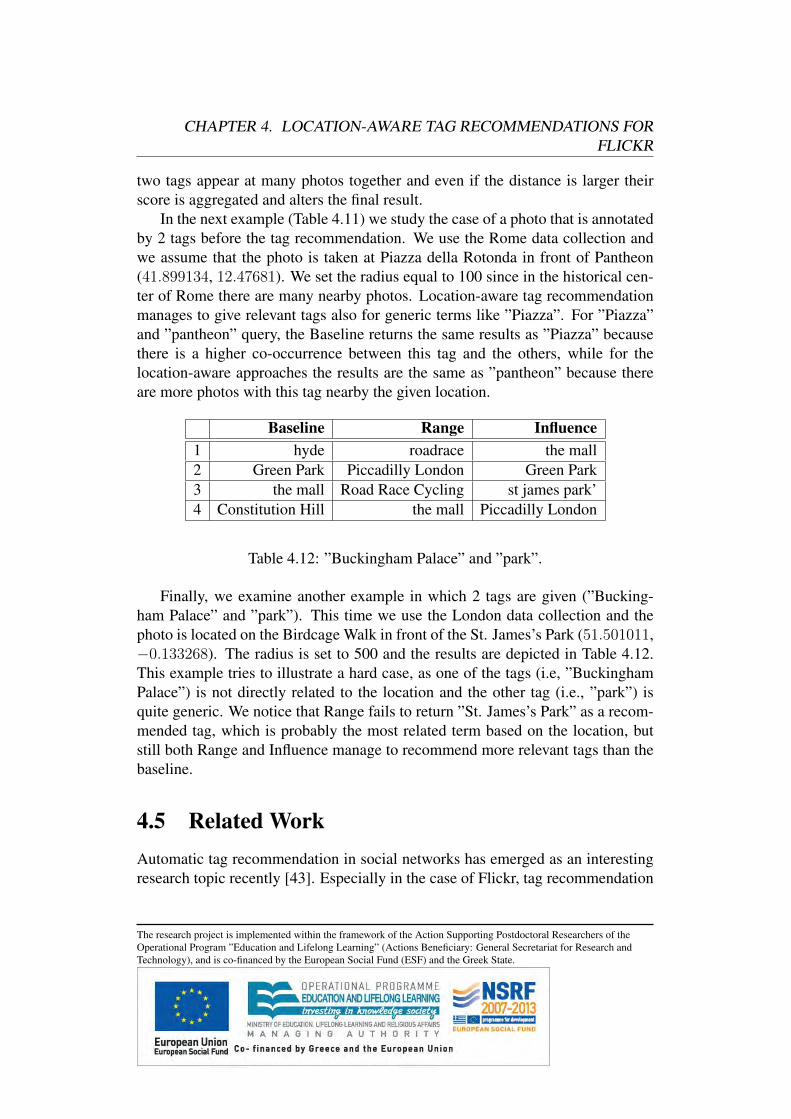
CHAPTER 4. LOCATION-AWARE TAG RECOMMENDATIONS FORFLICKR
two tags appear at many photos together and even if the distance is larger theirscore is aggregated and alters the final result.
In the next example (Table 4.11) we study the case of a photo that is annotatedby 2 tags before the tag recommendation. We use the Rome data collection andwe assume that the photo is taken at Piazza della Rotonda in front of Pantheon(41.899134, 12.47681). We set the radius equal to 100 since in the historical cen-ter of Rome there are many nearby photos. Location-aware tag recommendationmanages to give relevant tags also for generic terms like ”Piazza”. For ”Piazza”and ”pantheon” query, the Baseline returns the same results as ”Piazza” becausethere is a higher co-occurrence between this tag and the others, while for thelocation-aware approaches the results are the same as ”pantheon” because thereare more photos with this tag nearby the given location.
Baseline Range Influence1 hyde roadrace the mall2 Green Park Piccadilly London Green Park3 the mall Road Race Cycling st james park’4 Constitution Hill the mall Piccadilly London
Table 4.12: ”Buckingham Palace” and ”park”.
Finally, we examine another example in which 2 tags are given (”Bucking-ham Palace” and ”park”). This time we use the London data collection and thephoto is located on the Birdcage Walk in front of the St. James’s Park (51.501011,−0.133268). The radius is set to 500 and the results are depicted in Table 4.12.This example tries to illustrate a hard case, as one of the tags (i.e, ”BuckinghamPalace”) is not directly related to the location and the other tag (i.e., ”park”) isquite generic. We notice that Range fails to return ”St. James’s Park” as a recom-mended tag, which is probably the most related term based on the location, butstill both Range and Influence manage to recommend more relevant tags than thebaseline.
4.5 Related WorkAutomatic tag recommendation in social networks has emerged as an interestingresearch topic recently [43]. Especially in the case of Flickr, tag recommendation
The research project is implemented within the framework of the Action Supporting Postdoctoral Researchers of theOperational Program ”Education and Lifelong Learning” (Actions Beneficiary: General Secretariat for Research andTechnology), and is co-financed by the European Social Fund (ESF) and the Greek State.
CHAPTER 4. LOCATION-AWARE TAG RECOMMENDATIONS FORFLICKR
has been studied in [42, 21]. In more details, [42] presents different tag recom-mendation strategies relying on relationships between tags defined by the globalco-occurrence metrics. On the other hand, in [21] tag recommendation methodsare studied that are personalized and use knowledge about the particular user’stagging behavior in the past. Nevertheless, none of the above methods takes intoaccount the locations of photos. SpiritTagger [33] is a geo-aware tag suggestiontool for photos, but the proposed approach relies on the visual content (such asglobal color, texture, edge features) of the photo and on the global and local tagdistribution. In contrast, our approach takes into account the tag co-occurrenceand the distance between the given and the existing photos.
An overview of the field of recommender systems can be found in [1]. Aframework that decouples the definition of a recommendation process from itsexecution and supports flexible recommendations over structured data has beenproposed in [27, 28]. Neighborhood-based tag recommendation is studied in [5].The neighborhood is defined based on a graph and tags are propagated throughexisting edges.
In [41] the authors also focus on geo-tagged photos and propose methods forplacing photos uploaded to Flickr on the World map. These methods rely on thetextual annotations provided by the users and predict the single location where theimage was taken. This work is motivated by the fact that users spend considerableeffort to describe photos [3, 42] with tags and these tags relate to locations wherethey were taken.
4.6 ConclusionsTag recommendation is a very important and challenging task, since it helps usersto annotate their photos with more meaningful tags, which in turn enables re-trieving relevant photos from large photos collections such as Flickr. Nowadays,more and more photos are geotagged, and therefore we investigate how to im-prove tag recommendation based on the spatial and textual information of thephotos. To this end, we analyzed the tags of geotagged photos collected fromFlickr and proposed two different location-aware tag recommendation methods.Our experiments show that location-aware tag recommendation is promising andthe location of a photo improves the quality of the recommendation. In the future,we aim to investigate in depth how different existing recommendation methodscan be improved by combining them with the photo locations.
The research project is implemented within the framework of the Action Supporting Postdoctoral Researchers of theOperational Program ”Education and Lifelong Learning” (Actions Beneficiary: General Secretariat for Research andTechnology), and is co-financed by the European Social Fund (ESF) and the Greek State.

4.6.1 AcknowledgmentsThis research work was developed in cooperation with Ioanna Miliou and the re-search results where published at:Ioanna Miliou, Akrivi Vlachou: Location-Aware Tag Recommendations for Flickr,DEXA (1) 2014: 97-104.
The research project is implemented within the framework of the Action Supporting Postdoctoral Researchers of theOperational Program ”Education and Lifelong Learning” (Actions Beneficiary: General Secretariat for Research andTechnology), and is co-financed by the European Social Fund (ESF) and the Greek State.
Bibliography
[1] G. Adomavicius and A. Tuzhilin. Toward the next generation of rec-ommender systems: A survey of the state-of-the-art and possible exten-sions. IEEE Transactions on Knowledge and Data Engineering (TKDE),17(6):734–749, 2005.
[2] R. Agrawal, A. Gupta, Y. Prabhu, and M. Varma. Multi-label learning withmillions of labels: recommending advertiser bid phrases for web pages. InProc. of WWW, pages 13–24, 2013.
[3] M. Ames and M. Naaman. Why we tag: motivations for annotation in mobileand online media. In Proceedings of ACM Conference on Human Factors inComputing Systems (CHI), pages 971–980, 2007.
[4] P. Bouros, S. Ge, and N. Mamoulis. Spatio-textual similarity joins. PVLDB,6(1):1–12, 2012.
[5] A. Budura, S. Michel, P. Cudre-Mauroux, and K. Aberer. Neighborhood-based tag prediction. In Proceedings of Extended Semantic Web Conference(ESWC), pages 608–622, 2009.
[6] X. Cao, G. Cong, B. Cui, C. S. Jensen, and Q. Yuan. Approaches to exploringcategory information for question retrieval in community question-answerarchives. ACM Transactions on Information Systems, 30(2):7, 2012.
[7] X. Cao, G. Cong, and C. S. Jensen. Retrieving top-k prestige-based relevantspatial web objects. PVLDB, 3(1):373–384, 2010.
[8] X. Cao, G. Cong, C. S. Jensen, and B. C. Ooi. Collective spatial keywordquerying. In Proc. of SIGMOD, pages 373–384, 2011.
[9] X. Cao, G. Cong, C. S. Jensen, and M. L. Yiu. Retrieving regions of interestfor user exploration. PVLDB, 7(9):733–744, 2014.
BIBLIOGRAPHY
[10] Y.-C. Chang, L. D. Bergman, V. Castelli, C.-S. Li, M.-L. Lo, and J. R. Smith.The Onion technique: Indexing for linear optimization queries. In Proc. ofInt. Conference on Management of Data (SIGMOD), pages 391–402, 2000.
[11] L. Chen, G. Cong, C. S. Jensen, and D. Wu. Spatial keyword query process-ing: An experimental evaluation. PVLDB, 6(3):217–228, 2013.
[12] Y. Choi, M. Fontoura, E. Gabrilovich, V. Josifovski, M. R. Mediano, andB. Pang. Using landing pages for sponsored search ad selection. In Proc. ofWWW, pages 251–260, 2010.
[13] S. Cholette, O. Ozluk, and M. Parlar. Optimal keyword bids in search-basedadvertising with stochastic advertisement positions. J. Optimization Theoryand Applications, 152(1):225–244, 2012.
[14] G. Cong, C. S. Jensen, and D. Wu. Efficient retrieval of the top-k mostrelevant spatial web objects. PVLDB, 2(1):337–348, 2009.
[15] Y. Du, D. Zhang, and T. Xia. The optimal location query. In Proc. of SSTD,pages 163–180, 2005.
[16] E. Erkut. The discrete p-dispersion problem. European Journal of Opera-tional Research, 46(1):48–60, 1990.
[17] I. D. Felipe, V. Hristidis, and N. Rishe. Keyword search on spatial databases.In Proc. of ICDE, pages 656–665, 2008.
[18] J. Finger and N. Polyzotis. Robust and efficient algorithms for rank joinevaluation. In Proc. of SIGMOD, pages 415–428, 2009.
[19] A. Fuxman, P. Tsaparas, K. Achan, and R. Agrawal. Using the wisdom ofthe crowds for keyword generation. In Proc. of WWW, pages 61–70, 2008.
[20] M. R. Garey and D. S. Johnson. Computers and Intractability: A Guide tothe Theory of NP-Completeness. Macmillan Higher Education, 1979.
[21] N. Garg and I. Weber. Personalized, interactive tag recommendation forflickr. In Proceedings of ACM Recommender System Conference (RecSys),pages 67–74, 2008.
The research project is implemented within the framework of the Action Supporting Postdoctoral Researchers of theOperational Program ”Education and Lifelong Learning” (Actions Beneficiary: General Secretariat for Research andTechnology), and is co-financed by the European Social Fund (ESF) and the Greek State.
BIBLIOGRAPHY
[22] V. Hristidis, N. Koudas, and Y. Papakonstantinou. PREFER: a system forthe efficient execution of multi-parametric ranked queries. In Proc. of Int.Conference on Management of Data (SIGMOD), pages 259–270, 2001.
[23] I. F. Ilyas, W. G. Aref, and A. K. Elmagarmid. Supporting top-k join queriesin relational databases. VLDB J., 13(3):207–221, 2004.
[24] I. F. Ilyas, G. Beskales, and M. A. Soliman. A survey of top-k query pro-cessing techniques in relational database systems. ACM Comput. Surv.,40(4):11:1–11:58, 2008.
[25] I. Kamel and C. Faloutsos. Hilbert R-tree: An improved R-tree using frac-tals. In Proc. of VLDB, pages 500–509, 1994.
[26] F. Korn and S. Muthukrishnan. Influence sets based on reverse nearest neigh-bor queries. In Proc. of SIGMOD, pages 201–212, 2000.
[27] G. Koutrika, B. Bercovitz, and H. Garcia-Molina. Flexrecs: expressing andcombining flexible recommendations. In Proceedings of ACM InternationalConference on Management of Data (SIGMOD), pages 745–758, 2009.
[28] G. Koutrika, B. Bercovitz, R. Ikeda, F. Kaliszan, H. Liou, and H. Garcia-Molina. Flexible recommendations for course planning. In Proceedings ofInternational Conference on Data Engineering (ICDE), pages 1467–1470,2009.
[29] Z. Li, K. C. K. Lee, B. Zheng, W.-C. Lee, D. L. Lee, and X. Wang. IR-tree:An efficient index for geographic document search. IEEE TKDE, 23(4):585–599, 2011.
[30] C.-Y. Lin, J.-L. Koh, and A. L. P. Chen. Determining (k)-most demandingproducts with maximum expected number of total customers. IEEE Trans.Knowl. Data Eng., 25(8):1732–1747, 2013.
[31] J. Lu, Y. Lu, and G. Cong. Reverse spatial and textual k nearest neighborsearch. In Proc. of SIGMOD, pages 349–360, 2011.
[32] Y. Lu, J. Lu, G. Cong, W. Wu, and C. Shahabi. Efficient algorithms and costmodels for reverse spatial-keyword k-nearest neighbor search. ACM Trans.Database Syst., 39(2):13, 2014.
The research project is implemented within the framework of the Action Supporting Postdoctoral Researchers of theOperational Program ”Education and Lifelong Learning” (Actions Beneficiary: General Secretariat for Research andTechnology), and is co-financed by the European Social Fund (ESF) and the Greek State.
BIBLIOGRAPHY
[33] E. Moxley, J. Kleban, and B. S. Manjunath. Spirittagger: a geo-aware tagsuggestion tool mined from flickr. In Proceedings of Multimedia InformationRetrieval, pages 24–30, 2008.
[34] A. Okabe, B. Boots, K. Sugihara, and S. N. Chiu. Spatial Tessellations:Concepts and Applications of Voronoi Diagrams. John Wiley and Sons Ltd.,New York, NY, 2000.
[35] P. Papadimitriou, H. Garcia-Molina, A. Dasdan, and S. Kolay. Output URLbidding. PVLDB, 4(3):161–172, 2010.
[36] S. Ravi, A. Z. Broder, E. Gabrilovich, V. Josifovski, S. Pandey, and B. Pang.Automatic generation of bid phrases for online advertising. In Proc. ofWSDM, pages 341–350, 2010.
[37] S. S. Ravi, D. J. Rosenkrantz, and G. K. Tayi. Heuristic and special casealgorithms for dispersion problems. Operations Research, 42(2):299–310,1994.
[38] J. B. Rocha-Junior, O. Gkorgkas, S. Jonassen, and K. Nørvag. Efficientprocessing of top-k spatial keyword queries. In Proc. of SSTD, pages 205–222, 2011.
[39] J. B. Rocha-Junior, A. Vlachou, C. Doulkeridis, and K. Nørvag. Efficientprocessing of top-k spatial preference queries. PVLDB, 4(2):93–104, 2010.
[40] K. Schnaitter and N. Polyzotis. Optimal algorithms for evaluating rank joinsin database systems. ACM Trans. Database Syst., 35(1), 2010.
[41] P. Serdyukov, V. Murdock, and R. van Zwol. Placing flickr photos on amap. In Proceedings of International ACM Conference on Research andDevelopment in Information Retrieval (SIGIR), pages 484–491, 2009.
[42] B. Sigurbjornsson and R. van Zwol. Flickr tag recommendation based oncollective knowledge. In Proceedings of International World Wide Web Con-ference (WWW), pages 327–336, 2008.
[43] Y. Song, L. Zhang, and C. L. Giles. Automatic tag recommendation al-gorithms for social recommender systems. ACM Transactions on the Web(TWEB), 5(1):4, 2011.
The research project is implemented within the framework of the Action Supporting Postdoctoral Researchers of theOperational Program ”Education and Lifelong Learning” (Actions Beneficiary: General Secretariat for Research andTechnology), and is co-financed by the European Social Fund (ESF) and the Greek State.
BIBLIOGRAPHY
[44] Y. Tao, V. Hristidis, D. Papadias, and Y. Papakonstantinou. Branch-and-bound processing of ranked queries. Inf. Syst., 32(3):424–445, 2007.
[45] G. Valkanas, A. N. Papadopoulos, and D. Gunopulos. SkyDiver: a frame-work for skyline diversification. In Proc. of EDBT, pages 406–417, 2013.
[46] A. Vlachou, C. Doulkeridis, Y. Kotidis, and K. Nørvag. Reverse top-kqueries. In Proc. of Int. Conf. on Data Engineering (ICDE), 2010.
[47] A. Vlachou, C. Doulkeridis, Y. Kotidis, and K. Nørvag. Monochromatic andbichromatic reverse top-k queries. IEEE Transactions on Knowledge andData Engineering, 23(8):1215–1229, 2011.
[48] A. Vlachou, C. Doulkeridis, K. Nørvag, and Y. Kotidis. Identifying the mostinfluential data objects with reverse top-k queries. PVLDB, 3(1-2):364–372,2010.
[49] A. Vlachou, C. Doulkeridis, K. Nørvag, and Y. Kotidis. Identifying the mostinfluential data objects with reverse top-k queries. PVLDB, 3(1):364–372,2010.
[50] A. Vlachou, C. Doulkeridis, K. Nørvag, and Y. Kotidis. Branch-and-boundalgorithm for reverse top-k queries. In Proc. SIGMOD, pages 481–492,2013.
[51] D. Wu, M. L. Yiu, G. Cong, and C. S. Jensen. Joint top-k spatial keywordquery processing. IEEE Trans. Knowl. Data Eng., 24(10):1889–1903, 2012.
[52] T. Xia, D. Zhang, E. Kanoulas, and Y. Du. On computing top-t most influ-ential spatial sites. In Proc. of VLDB, pages 946–957, 2005.
[53] M. L. Yiu, X. Dai, N. Mamoulis, and M. Vaitis. Top-k spatial preferencequeries. In Proc. of ICDE, pages 1076–1085, 2007.
[54] M. L. Yiu, H. Lu, N. Mamoulis, and M. Vaitis. Ranking spatial data byquality preferences. IEEE TKDE, 23(3):433–446, 2011.
[55] D. Zhang, Y. M. Chee, A. Mondal, A. K. H. Tung, and M. Kitsuregawa.Keyword search in spatial databases: Towards searching by document. InProc. of ICDE, pages 688–699, 2009.
The research project is implemented within the framework of the Action Supporting Postdoctoral Researchers of theOperational Program ”Education and Lifelong Learning” (Actions Beneficiary: General Secretariat for Research andTechnology), and is co-financed by the European Social Fund (ESF) and the Greek State.

BIBLIOGRAPHY
[56] W. Zhang, D. Wang, G.-R. Xue, and H. Zha. Advertising keywords recom-mendation for short-text web pages using Wikipedia. ACM TIST, 3(2):36,2012.
The research project is implemented within the framework of the Action Supporting Postdoctoral Researchers of theOperational Program ”Education and Lifelong Learning” (Actions Beneficiary: General Secretariat for Research andTechnology), and is co-financed by the European Social Fund (ESF) and the Greek State.


![[K. W. Arafat] Pausanias' Greece Ancient Artists (BookFi.org)](https://img.dokumen.tips/doc/110x75/55cf9d25550346d033ac6ca0/k-w-arafat-pausanias-greece-ancient-artists-bookfiorg.jpg)