Paul Cheshire, Christian A.L. Hilber and Hans R.A. Koster

Empty homes, longer commutes: the unintended consequences of more restrictive local planning Article (Published version) (Refereed)

Original citation: Cheshire, Paul and Hilber, Christian A.L. and Koster, Hans R.A. (2018) Empty homes, longer commutes: the unintended consequences of more restrictive local planning. Journal of Public Economics, 158. pp. 126-151. ISSN 0047-2727 DOI: 10.1016/j.jpubeco.2017.12.006 © 2018 the Authors CC BY 4.0 This version available at: http://eprints.lse.ac.uk/86441/ Available in LSE Research Online: August 2018 LSE has developed LSE Research Online so that users may access research output of the School. Copyright © and Moral Rights for the papers on this site are retained by the individual authors and/or other copyright owners. Users may download and/or print one copy of any article(s) in LSE Research Online to facilitate their private study or for non-commercial research. You may not engage in further distribution of the material or use it for any profit-making activities or any commercial gain. You may freely distribute the URL (http://eprints.lse.ac.uk) of the LSE Research Online website.

Contents lists available at ScienceDirect

Journal of Public Economics

journal homepage: www.elsevier.com/locate/jpube

Empty homes, longer commutes: The unintended consequences of morerestrictive local planning☆

Paul Cheshirea, Christian A.L. Hilbera, Hans R.A. Kosterb,c,d,⁎

a London School of Economics, Centre for Economic Performance, Spatial Economics Research Centre, United Kingdomb Vrije Universiteit Amsterdam, Tinbergen Institute, The Netherlandsc Centre for Economic Policy Research, Spatial Economics Research Centre, United KingdomdNational Research University, Higher School of Economics, Russian Federation

A R T I C L E I N F O

JEL classification:R13R38

Keywords:Residential vacancy ratesHousing supply constraintsLand use regulation

A B S T R A C T

We investigate the impact of land use regulation on housing vacancy rates. Using a 30-year panel dataset on landuse regulation for 350 English Local Authorities (LAs) and addressing potential reverse causation and otherendogeneity concerns, we find that tighter local planning constraints increase local housing vacancy rates: a onestandard deviation increase in restrictiveness causes the local vacancy rate to increase by 0.9 percentage points(23%). The same increase in local restrictiveness also causes a 6.1% rise in commuting distances. The resultsunderline the interdependence of local housing and Labour markets and the unintended adverse impact of morerestrictive planning policies.

1. Introduction

To an economist it might seem self-evident that vacancies in thehousing stock are a natural feature of how any market must work. Thereeven are ‘uneaten’ apples in a well-functioning fruit market. The Labourmarket is very much more comparable to the housing market and vir-tually all mainstream economists expect to observe at least frictionalunemployment when the Labour market is in equilibrium (seePissarides, 1985; Mortensen and Pissarides, 1994; Pissarides, 1994). Itis the same in any normally functioning housing market. In equilibriumthere must be vacant houses as people move and ‘house-hunt’, as peopledie or houses wait to be demolished and sellers wait to find a buyer(Han and Strange, 2015).

But this view is often not shared by those who design buildings andinfluence urban policy or with those who plan housing supply – at leastin England. Even in what was then one of the least restrictive EnglishRegions, the East Midlands, in calculating how much land should beallocated for housing to meet their estimate of their region's ‘housing

needs’, planners argued that they could allocate less land because theyassumed they would reduce the number of vacant homes:

‘The annual average housing provision reflects a number of factors,transactional vacancies in new stock (about 2%) add 7,000 to the re-quirement, but offset against that is an assumption that vacancies in theexisting stock should be reduced by a half per-cent, which will bring8,600 dwellings back into use.’ (Government Office for the EastMidlands, 2005, Appendix 4, p. 91).

It is surely true that using ones stock of capital more intensively is away of increasing efficiency. That is just how cut price airlines operate:they keep their seats full and their aircraft in the air. They, however,had an analysis of how to achieve this. They did not just assume planeswould spend more of their lives in the air and seats would be fuller.Unless we understand why houses are vacant we cannot rationally hopeto reduce the number of vacant houses just by being more restrictive.To help improve our understanding of the factors which determinevacancy rates in the housing market, this paper investigates the causal,

https://doi.org/10.1016/j.jpubeco.2017.12.006Received 23 May 2016; Received in revised form 1 September 2017; Accepted 19 December 2017

☆ The research formed part of the programme of the Spatial Economics Research Centre (SERC) funded by grants from the UK Economic and Social Research Council (ES/J021342/1),the UK Government Department of Business Innovation and Skills, and the Welsh Advisory Government. We also benefited from the support from the Suntoya and Toyota InternationalCentres for Economics and Related Disciplines (STICERD). Both funders are gratefully acknowledged. Hans Koster acknowledges support from a VENI research grant from the NetherlandsOrganisation for Scientific Research (451-14-034). We thank Gabriel Ahlfeldt, Jan Brueckner, Ed Coulson, Jeremiah Dittmar, Gilles Duranton, Stuart Gabriel, Steve Gibbons, RavenMolloy, Alvin Murphy, Henry Overman, Olmo Silva, Stuart Rosenthal, Will Strange, Jos Van Ommeren, Elisabet Viladecans-Marsal, Stephen Ross and conference/seminar participants atthe Urban Economics Association Meetings of the 2013 North American Meetings of the RSAI (Atlanta) and of the 2015 European Regional Science Association Congress (Lisbon), the2015 AREUEA National Conference (Washington, DC), the 2015 Conference on Housing Affordability at the UCLA (Los Angeles), the 2015 CEPR Conference on Urban and RegionalEconomics (CURE) (Basel), the 2016 AREUEA-ASSA Conference (San Francisco), the Urban and Regional Economics seminar (Paris) and the SERC/LSE seminar (London) for helpfulcomments and suggestions. All errors are the sole responsibility of the authors. We also thank the Editor and two anonymous referees for helpful comments and suggestions.

⁎ Corresponding author at: Vrije Universiteit Amsterdam, De Boelelaan 1105, 1081 HV Amsterdam, The Netherlands.E-mail addresses: p.cheshire@lse.ac.uk (P. Cheshire), c.hilber@lse.ac.uk (C.A.L. Hilber), h.koster@vu.nl (H.R.A. Koster).

Journal of Public Economics 158 (2018) 126–151

Available online 26 December 20170047-2727/ © 2018 The Authors. Published by Elsevier B.V. This is an open access article under the CC BY license (http://creativecommons.org/licenses/BY/4.0/).

T

albeit reduced-form, impact of regulatory restrictiveness. Moreover,since housing and Labour markets are interdependent, we also in-vestigate the related issue of how local regulatory restrictiveness affectsthe average commute distance of those working in the jurisdiction.These are not the only outcomes of greater regulatory restrictiveness.We find that there are other measurable effects apart from raised houseprices, all apparently responses to poorer housing market matching(discussed below); more households are in temporary homes, crowdingis greater, and in-migration lower.

These results stem from the insight that policy imposed restrictionson housing supply may have two opposing effects.1 The first of these wecall the ‘opportunity cost effect’. Tighter restrictions on supply implyfewer available houses and therefore more demand pressure for existinghomes, increasing house prices and thus the opportunity cost of keepinghousing empty. This will lead to a lower vacancy rate all else equal. Ifthis ‘opportunity cost effect’ was the only effect at work, tighter supplyconstraints should unambiguously lower vacancy rates.

There is however a second effect, which we refer to as the ‘mismatcheffect’. Tighter supply constraints not only reduce supply of new housesbut also influence the composition and adaptability of the bundle ofattributes of both the existing housing stock and those of new builthomes. Over time the structure of households' demand for housing at-tributes changes because incomes rise, the demographic structure of thepopulation changes and preferences themselves may change. For ex-ample, as real incomes rise, so does the demand for certain attributesdepending on the varying income elasticity of demand for them.2 Inaddition there may be demographic changes such as an increase in theproportion of single adults, which mean that market preferenceschange.

If the attributes of the housing stock, as a consequence of planningconstraints, cannot, or can only more slowly adjust to these changes onthe demand side, matching the demand for housing attributes with thesupply of those available will inevitably become more difficult. Hence,in line with Wheaton (1990), mismatched households may have to staylonger in a less restrictive housing market while searching in a morerestrictive one, implying a relatively lower vacancy rate in the less re-strictive market and a higher vacancy rate in the more restrictive one.Mismatched households may also take temporary accommodation andsearch for longer in more restrictive markets or have to search furtherafield for a suitable home; they become mismatched on the locationalcharacteristics of houses implying longer commutes.

Our aim in this paper is to determine the net effect of these twoopposing forces – the opportunity cost effect versus the mismatch effect– in order to identify the role that regulatory restrictiveness plays indetermining the vacancy rate in local housing markets. To do so, weanalyse panel data on housing vacancies from 1981 to 2011 for 350English Local Authorities (LAs), the basic local jurisdictional unit thatimplements planning policies and approves or rejects individual plan-ning applications. One key concern in this analysis is the endogeneity oflocal planning restrictiveness. The stylised fact that policy makers andlocal planners may respond to higher vacancy rates by restrictingsupply suggests possible reverse causation. Regulatory constraints mayalso be endogenous to unobserved demand factors (Hilber and Robert-Nicoud, 2013; Davidoff, 2016) and those demand factors may directlyaffect vacancy rates. To account for possible reverse causation andomitted variable bias and thus identify the causal effect of regulatory

restrictiveness, we employ an instrumental variable strategy by ex-ploiting specific features of the British voting system which induces asubstantial ‘randomness’ of seats won (or lost) beyond the vote share.That is, we use the share of Labour seats in LAs, controlling for the shareof Labour votes in a flexible way, as an instrumental variable to identifylocal planning restrictiveness. One could query this identificationstrategy because, for example, the political composition of an LA couldinfluence local government expenditures and those, in turn, might in-fluence house prices and vacancy rates. Based on a series of placeboregressions, we show that these alternative explanations do not plau-sibly invalidate the main conclusions.

Our two key empirical findings are as follows. First, when we na-ively look at cross-sectional data, we find a negative relationship be-tween more restrictive local planning and local vacancy rates, super-ficially appearing to confirm “planners' assumptions”. However, whenwe (i) use first differencing and so control for time-invariant un-observable characteristics, (ii) properly account for the endogeneity ofrestrictiveness by instrumenting for it and (iii) control for other relevantfactors, more restrictive places have a significantly – and substantially –higher vacancy rate. That is, the underlying causal relationship appearsto be exactly the opposite to that which planners assume. Based on ourmost rigorous empirical specification, a one standard deviation increasein local regulatory restrictiveness causes the average local vacancy rateto increase by about 0.9 percentage points (23%).

Second, we find that regulation-induced mismatch has spatial im-plications for Labour markets. Workers with jobs in LAs with morerestrictive planning have to search for housing they can afford andmatch their preferences further afield; so they are more likely to belocationally mismatched and have to commute further. Using a similarapproach to that used for investigating the underlying relationshipbetween the vacancy rate and restrictiveness we find that a one stan-dard deviation increase in local regulatory restrictiveness causes anincrease in average commuting distance of some 6.1%. We also provideadditional suggestive evidence relating to other proxies for mismatch,such as the share of crowded or non-permanent properties and the shareof migrants.

Our findings, therefore, strongly suggest that tighter local planningrestrictiveness not only leads to less efficient housing market matchingbut also this effect dominates the opportunity cost effect, resulting inhigher local vacancy rates overall and longer average commutes.Hence, local efforts to reduce the number of vacant homes by imposingsupply restrictions have three unintended effects: they increase thelocal vacancy rate and they increase the average commuting distance ofthose who work in the jurisdiction – thereby causing a welfare cost. Inaddition, as the literature shows, they increase local house prices (seee.g. Cheshire and Sheppard, 2002; Glaeser and Gyourko, 2003; Hilberand Vermeulen, 2016).

We proceed as follows. In the next section we discuss in more depththe link between land use regulation and mismatch in the housingmarket and how that affects the local vacancy rate and the averagecommuting distance. We then describe our data and set out our mainresults. The final section draws conclusions.

2. Land use regulation, housing market search and vacant housing

The price of housing services is a function of both demand andsupply in the relevant local markets. Various empirical studies docu-ment a positive effect of regulatory restrictiveness on house prices(Cheshire and Sheppard, 2002; Glaeser and Gyourko, 2003; Glaeseret al., 2005a, 2005b; Quigley and Raphael, 2005; Ihlanfeldt, 2007;Hilber and Vermeulen, 2016).

What these studies do not consider is the fact that, on the seller'sside, it takes time to sell a house and, on the buyer's side, search for anew house is costly too. These search frictions lead to housing vacancies(Merlo and Ortalo-Magné, 2004; Han and Strange, 2015). It has beendocumented – and our data also suggest – that housing vacancies are

1 Regulation may have more than two effects. We discuss one potential additionalmechanism – a real options argument – in Section 3.7. If greater restrictiveness led togreater price volatility then under certain assumptions this might induce owners topostpone renting or selling their properties, implying a higher vacancy rate (Grenadier,1995, 1996). Empirically, however, we can find no evidence that such a mechanism playsa significant part in explaining what we find. Other mechanisms are also discussed in thatsection.

2 The income elasticity of demand for space both inside houses and in gardens seems tobe particularly strong: Cheshire and Sheppard (1998) estimate an elasticity of close totwo.

P. Cheshire et al. Journal of Public Economics 158 (2018) 126–151

127

not constant across space and time and depend on the characteristicsand preferences of households living in a housing market, as well as onthose of the location such as characteristics that are systematic ofpersistently weak housing demand (Rosen and Smith, 1983; Gabriel andNothaft, 1988; Gabriel and Nothaft, 2001; Deng et al., 2003; Molloy,2016). However, the impact of land use restrictions on housing va-cancies has not yet been studied.

In the context of this paper we use data on local jurisdictions – inBritain, LAs – which we refer to as local housing markets.3 On the de-mand side, households often search in a local housing market while stillliving in another local market, for example due to changes in wherethey work (Mulalic et al., 2014; Koster and Van Ommeren, 2017). Onthe supply side, the characteristics of housing are the result of both thecharacteristics of new build housing and the adaptation of the char-acteristics of the existing stock.

The degree of regulatory restrictiveness influences the character-istics of new construction and of the existing stock in very great detail.Both new construction and significant changes to the characteristics ofexisting houses – converting loft to living space, for example – likelyrequire ‘development control’ permission. This is the responsibility ofthe LA's Planning Committee made up of locally elected politicians. Thisdecision making process tends to be politicised and unlike a Zoning orMaster Planning system, such as in force in the US or in most ofContinental Europe, decisions are not very predictable.

As noted in the introduction, planning induced housing supply re-strictions will have two opposing effects on the housing vacancy rate:an ‘opportunity cost effect’ and a ‘mismatch effect’. The opportunitycost effect works via restrictions of supply reducing the availability ofland for development (see for example Cheshire and Sheppard, 2005, orHilber and Vermeulen, 2016). This reduces the rate of new building andso over time the size of the stock of housing relative to demand withinthe market. This, all else equal, increases prices and thus the opportu-nity cost of keeping housing vacant. The effect of this is unambiguouslyto reduce vacancy rates. It will also be likely to increase price volatility.

However, more restrictive planning policies will also change thebundle of attributes on offer and, other things equal, slow the rate ofadaptation of housing characteristics to changes in the structure ofdemand with respect to them – the mismatch effect. The latter effect isexpected to increase vacancy rates. This will come about via two se-parate forces, one working on the characteristics of new build and theother on the adaptation of the characteristics of the existing stock ofhouses.

The first force may imply that new build houses become smaller,more distant from jobs and are more likely to be in the form of flats orterraced houses, because there is less land available for dwellings. Thesecond force arises because the structure of demand for housing char-acteristics changes over time and to accommodate this, the character-istics of the existing stock of housing need to be constantly adjusted. Forexample, entry to the best state schools in Britain is determined by theexact location of houses. As the relative standing of different schoolschanges over time, people seeking to ‘buy’ entry to better state schoolswill want more bedroom space in the best schools' catchment areas.However, the more restrictive is the LA, the more difficult it will be toadapt existing houses to provide more space or for developers to buildadditional family housing near better schools.

Another example is that as more cars have been bought (car own-ership has increased 13-fold since the current form of land use planning

in England was introduced in 1947 and doubled since our vacancy datastarts in 1981, Department of Transport, 2013), the demand for garagesand off street parking has increased. Such examples of ways in whichthe demand for housing attributes changes over time could be increasedalmost indefinitely. However, what it means is that if the supply anddemand for the structural characteristics of housing are to be efficientlymatched to each other, there will need to be constant adaptation of thecharacteristics of the existing stock of houses. So more restrictive LAswill slow the adaptation of the existing stock to (changes in) thestructure of demand for housing attributes.

Over time, in more restrictive LAs the characteristics of new andexisting housing available will be less adapted to preferences ofhouseholds. Hence, other things equal, if people have a (strong) idio-syncratic preference for locations and house type (e.g. a double-earnerhousehold with children that needs at least two-bedrooms and gardenspace), they will spend more time searching for housing that matchestheir preferences. When households live in a less restrictive housingmarket while searching in the more restrictive local market, this willimply a decrease in the vacancy rate in the former and an increase inthe latter housing market.4 In other words, given idiosyncratic pre-ferences, households stay longer in the ‘wrong’ places.

This may imply that younger people live longer with their parents in‘crowded’ properties, or that households are induced to stay in tem-porary accommodation while searching. Because the housing stock doesnot match their current preferences, this implies a higher vacancy rate,other things equal, in the more restrictive housing market. We providesome evidence on some of these different symptoms of mismatch inSection 3.6 where we look at how regulation influences the share ofnon-permanent homes and ‘crowded’ properties.

We discuss also a more obvious measure of mismatch in Section 3.4:commuting distances from the workplace in the LA. We do indeed findthat for workers in more restrictive LAs commuting distances increasesignificantly. This result is consistent with house hunters finding it moredifficult to match their preferences in more restrictive local housingmarkets so becoming ‘mismatched’ locationally. This has interestingimplications for the boundaries of local Labour markets – they appear tobe determined not just by transport costs but also by local planningpolicies – and how these affect the total supply of housing and thesupply of individual housing characteristics. Because households maydecide not to move to the desired more restricted place, the share of in-migrants is expected to be lower in the more restrictive housing market.We provide evidence for the latter in Section 3.6.

The well-documented fact that tighter local regulation leads tohigher prices is indicative that the opportunity cost effect may be im-portant in determining local vacancy rates. However, we lack evidenceon the importance of the offsetting mismatch effect. Thus the net effectof local regulatory restrictiveness on local vacancy rates is ambiguous.The empirical analysis that follows aims to identify this net effect whileeliminating alternative explanations.

One may question whether changes in vacancy rates are a sufficientstatistic when one is interested in the welfare effects of land use reg-ulation. We do not argue that vacancy rates in general are a sufficientstatistic. However, when one is specifically interested in the change inwelfare due to an increase in mismatch caused by more restrictive localplanning, an increase in the vacancy rate (beyond the natural rate) is asufficient statistic for the former.

In line with a large Labour market literature on matching, and asdemonstrated by Koster and Van Ommeren (2017), from a welfareperspective housing search may be either too low or too high. However,

3 It might be argued that Travel to Work Areas (TTWA) approximate more closely tospatial housing markets but as our results demonstrate, the geographical extent of bothhousing and Labour markets is jointly determined. Planning policy is implemented by thelocal jurisdiction, the LA, so it is only by using these as our units of analysis that therelationship between restrictiveness and commuting distances can be revealed. Not onlydo TTWAs not correspond to any political jurisdiction but our finding on the impact ofplanning restrictiveness on distance commuted shows their boundaries are partially de-termined by the policy actions of their constituent jurisdictions.

4 In the Web Appendix we demonstrate this in a standard search model setting,building on the seminal paper by Wheaton (1990). Using numerical simulations, weformally demonstrate that under realistic parameter assumptions an increase in the (re-lative) regulatory restrictiveness in a particular market increases the local vacancy rate inthat market (and lowers it in the comparably less restrictive market), even with perfectlyinelastic total demand for housing.

P. Cheshire et al. Journal of Public Economics 158 (2018) 126–151

128

when search is too low, that is caused by an externality for sellers: ifbuyers search more they will find a suitable property sooner, therebyreducing the time on the market and the associated costs for the seller.Buyers do not take this into account when increasing search effort.However, a regulation-induced increase in vacancy rates while in-creasing search effort, neither reduces sales times, nor increasesmatching quality, so the welfare effects are unambiguously negative.

This is important because planning policies that aim to reduce va-cancies by reducing new construction but end up leaving more housesempty, cause an under-utilisation of a major capital asset. According toONS by the end of 2013 houses accounted for 61% of the UK's networth: up from 48.7% 20 years previously (ONS, 2016). So the capitalstock represented by housing is very significant indeed and so its un-derutilisation represents a significant economic inefficiency.

The effects on commuting are important in their own right as againthey represent a welfare loss resulting from increased difficulty ofmatching.

Of course planning policies per se have the potential to increasesocial welfare via correcting market failures and we are not claiminghere that our evidence on the effect of land use regulation on vacancyrates and commuting distances in isolation suggests that local planningrestrictions reduce net welfare. However, there is evidence at least forthe UK and the US that an increase in the restrictiveness of planningpolicy (from current levels) has a net negative effect on welfare (seeCheshire and Sheppard, 2002 for the UK and Turner et al. (2014) for theUS). In this context, our finding that more restrictive local planningincreases the local vacancy rate and commuting distance via raisingmismatch in the local housing market, adds to the alleged net negativeeffect on welfare. Both effects (on vacancy rates and commuting dis-tances) have been ignored in the literature so far.

3. Empirical analysis

3.1. Data and descriptive statistics

Our data come from several sources. The vacancy rates are from theUK Census for the years 1981, 1991, 2001 and 2011.5 For the first threeCensus years we have information on the number of vacant dwellingsand we are able to distinguish between primary dwellings and secondhomes.6 The 2011 Census reported only information on the number ofunoccupied dwellings including second homes. To estimate vacancies for2011 in the most consistent way possible, therefore, we assume that theshare of second homes remained constant between 2001 and 2011. In arobustness check we use an alternative dataset for vacancy rates(available for 2001 and 2011 only) to test whether our findings aresensitive to this adjustment. The latter dataset is provided by the De-partment of Communities and Local Government (DCLG) using the LAreturns for the Council Tax.7

Our measures of regulatory restrictiveness come from the DCLG's

Planning Statistics. Following the literature, our key measure is therefusal rate for major residential projects available for each LA on anannual basis. The refusal rate for ‘major’ projects is defined as the shareof applications for residential developments of ten or more dwellingsthat is refused by an LA in any year during the process of ‘developmentcontrol’. We calculate this for each LA using data on all applications andrefused applications of major developments for the Census year itselfplus the two years preceding it.8 In what follows we call this variablethe refusal rate.

As a proxy for local (housing) demand we use LA-level male weeklyearnings for the period from 1981 to 2011. Our earnings data comefrom the Annual Survey of Hours and Earnings (ASHE) for 2001 and2011 and from the New Earnings Survey (NES) for 1981 and 1991. Weobtained the ASHE data at the LA-level but the NES data for earlieryears are only available at the county and London borough level. Wethen geographically matched all earnings data to the LA-level and de-flated the nominal earnings figures by the Retail Price Index to obtainreal earnings. For more details on the data and procedures used, seeHilber and Vermeulen (2016).

A number of other factors may influence vacancy rates, in particularhousing tenure, demographics and socio economic characteristics. Weobtain these control variables from the Population Censuses. Our list ofcontrols includes the local homeownership rate. Homeowners tend tomove less often than renters, and this is likely to be reflected in highervacancy rates for rental housing. We also control for the share ofcouncil housing. Because rents of council houses are usually belowmarket value, there are waiting lists for them. This is likely to imply ashorter duration of vacancies (Pawson and Kintrea, 2002). However,this effect could be offset to the extent councils have less efficienthousing management.

The Population Censuses also provide data on the share of peoplebetween 30 and 64 and the share of elderly, 65 and over. Young peoplemay be more flexible in their housing choices than older people, andthey may be less selective because they are more income constrained orhave lower search costs (perhaps because of lower opportunity costs oftime) leading to lower vacancy rates in LAs where there are pro-portionately more young adults. On the other hand, younger peopletend to have a higher mobility rate, leading to higher vacancy rates. Themortality rate is of course highly correlated to the share of elderly.Death frequently implies that houses become vacant and, moreover,because of probate and perhaps other reasons (the new owner may notbe a local resident or the house has suffered a period of neglect so ismore likely to need refurbishment) houses that become vacant on thedeath of their owner are likely to remain vacant for longer. Othercontrol variables derived from the Population Censuses are the shareunemployed, the share of highly educated, and the share of residentswith permanent illnesses.

As a proxy for mismatch and as a significant focus of interest in itsown right, we gather data on the average commuting distance from theworkplace for all the Census years. The data provide us with the shareof people per commuting distance band (0–2 km, 2–5 km, etc.). Wethen calculate the average commuting distance by taking the midpointof each category and weighting it by the number of persons in eachcategory. We further gather data on other variables that may relate tospatial mismatch from the Census, such as the share of crowded prop-erties, the share of shared properties, the share of migrants and theshare of non-permanent dwellings.

Our instrumental variable strategy employs information on the po-litical composition of the LA and local vote shares. We obtained thelocal election data from various sources: (i) the British Local ElectionDatabase (1889–2003) compiled by Rallings and Thrasher (2004), (ii)

5 The Census does not distinguish between short-term and long-term vacant housingunits. Molloy (2016) points out that in the United States, long-term vacancies are onaverage rare but there are substantial spatial differences. Our data do not allow us toexplore differences between short-term and long-term vacancies. However, it is worthpointing out that due to the extremely inflexible planning system in England, over-building is highly unlikely anywhere in the country. Long-term vacancies as a con-sequence of weak housing demand will likely be concentrated in the north of the countryand the change in the unemployment rate will likely capture the effect of declining areasin our empirical analysis.

6 The Census uses the term ‘household space’, which is a space taken by one household,including that of just one person. Almost no household shares facilities like bathrooms(< 0.1%), implying that the number of (vacant) household spaces is essentially the sameas the number of (vacant) dwellings. Hence, in what follows, we will refer to dwellings ashousehold spaces.

7 The cross-sectional correlation between the 2001 Census and the DCLG data is 0.68,indicating that there are non-trivial differences in the measurement of vacant dwellingsarising from the different methodologies. As is discussed later, this hardly affects ourresults however.

8 In a sensitivity analysis – see Appendix 2 – we also use additional information on therefusal rate of minor projects and show that our results are robust when we include thisadditional information.

P. Cheshire et al. Journal of Public Economics 158 (2018) 126–151

129

the Local Election Handbooks (1999 to 2008), (iii) the Local ElectionsArchive Project (LEAP) (2006 to 2010) and (iv) the BBC (2009 to 2011).We do not have data on four LAs, so these are excluded from the ana-lysis, leaving us with a sample of 350 LAs and four Census years (1981,1991, 2001 and 2011).9 Since it might be argued that turnout is un-representatively low at local elections in the sensitivity analysis, wealso use data on general elections, by matching each Census year to thenearest general election year (i.e., 1983, 1992, 2001 and 2010). The LA-level share of votes for the Labour party in the general elections isderived from the British Election Studies Information System. For moreinformation on the election data, see Appendix 1.

We also gather data on net local expenditures from the CharteredInstitute for Public Finance and Accountancy (CIPFA) annual reports onfinance and general estimates available for each LA. We choosespending categories that remain robust over time, such as spending oneducation, personal and social services (such as social care), highways,housing services, local planning and the total local net expenditures.Because these are net expenditures, they may be negative in certaininstances. We express the local expenditures in £ per head of the po-pulation. We note that for education, personal and social services, andhighways, the largest share of the spending is done at the county level.Although LAs have some freedom to spend extra money, we add the netspending per head at the county level to the local expenditures in thesecategories (otherwise most values would be zero). This also explainswhy the total local expenditures of an LA are lower than, for example,the net spending on education: the total expenditures only refer toexpenditures by the LA itself. In a few instances data are missing forindividual LAs (in particular for a dozen LAs in Greater London in1981). In cases such as this we impute the missing values from theaverage spending in a county, implying (a small) measurement error.However, in the placebo regressions in Section 3.4 the spending is thedependent variable. As long as this measurement error is random, itdoes not affect the estimated coefficients.

We obtained data on house prices from the Land Registry(1995–2011) and the Council of Mortgage Lenders (CML) (1974–1995).We do so by taking account of the composition of sales in terms ofhousing types by adopting a mix-adjustment approach (see Wall, 1998).The real price index is obtained by again deflating the nominal serieswith the Retail Price Index. We then use the price index to create ameasure of local price volatility; for more information see Hilber andVermeulen (2016).

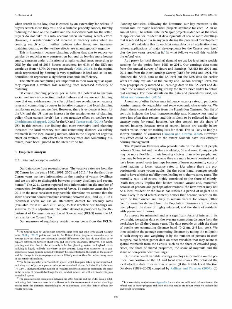
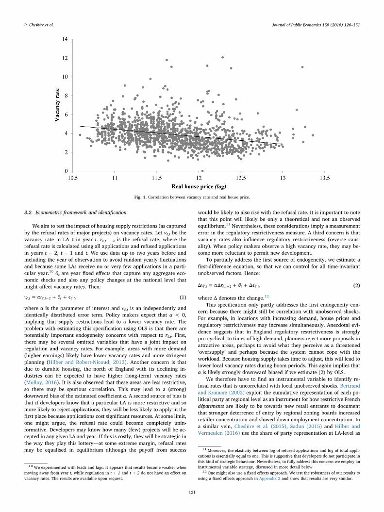
Table 1 presents the descriptive statistics. The average overall va-cancy rate is about 4%. The vacancy rate in 2011 was 3.6%. This is onlyslightly lower than in the United States, where it was 4.5% in 2012.This might seem surprising when one takes into account the enormousexcess supply of housing in the wake of the Great Recession that madehousing extremely affordable in the US. In Fig. 1 we plot the cross-sectional relationship between the vacancy rate and house prices. Va-cancy rates are somewhat lower in areas with high prices(ρ =−0.246), consistent with the opportunity cost argument discussedabove. There is little response to the housing market cycle; the corre-lation between the change in the vacancy rate and the change in houseprices is very low with ρ= −0.069.

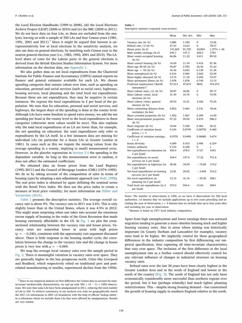
We map the average local vacancy rates over the sample period inFig. 2. There is meaningful variation in vacancy rates over space. Theyare generally higher in the less prosperous north. Cities like Liverpooland Bradford, which respectively relied on traditional port and port-related manufacturing or textiles, experienced decline from the 1950s.

Apart from high unemployment and lower earnings there was outwardmigration tending to generate a more obsolete housing stock and higherhousing vacancy rates. Also in areas where mining was historicallyimportant (in County Durham and Lancashire for example), vacancyrates tend to be higher. We implicitly control for these geographicaldifferences in the industry composition by first differencing our em-pirical specification, thus capturing all time-invariant characteristicsthat vary over space. The inclusion of the first difference in the localunemployment rate as a further control should effectively control forany relevant influence of changes in industrial structure on housingvacancy rates.

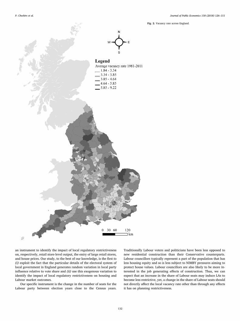
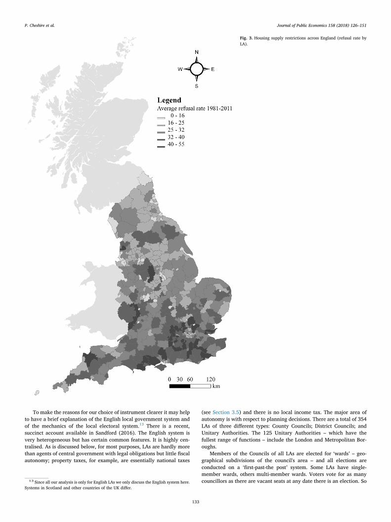
Refusal rates over the last 30 years have been clearly highest in theGreater London Area and in the south of England and lowest in thenorth of the country (Fig. 3). The south of England has not only beeneconomically considerably more successful than northern regions overthe period, but it has (perhaps relatedly) had much tighter planningrestrictiveness. This – despite strong housing demand – has constrainedthe growth of housing supply in southern England relative to the north.

Table 1Descriptive statistics (repeated cross-section).

Mean Std. dev. Min Max

Vacancy rate (in %) 3.886 1.340 0 12.06Refusal rate, t-2 (in %) 27.43 14.63 0 78.57House price (in £) 141,665 91,729 43,804 1.277e + 06Male weekly earnings (in £) 545.7 147.3 258.3 1793Share owner-occupied housing

(in %)66.86 11.22 4.611 89.52

Share council housing (in %) 16.09 11.34 0.416 81.96Share age 30–65 (in %) 44.87 2.783 36.42 51.62Share age > 65 (in %) 16.42 3.642 6.128 31.36Share unemployed (in %) 6.516 2.960 2.042 22.40Share highly educated (in %) 13.74 11.39 0.244 53.57Share permanent illness (in %) 3.478 1.878 0.745 12.15Predicted employment (‘Bartik

instrument’)a57,913 47,674 9832 474,473

Share Labour seats, t-2, (in %) 30.87 26.86 0 99.17Share Labour voters, local

elections (in %)31.49 16.76 0 76.95

Share Labour voters, generalelection (in %)

29.53 15.21 2.426 75.25

Mean commuting distance fromworkplace (in km)

6.853 3.465 2.141 18.66

Share crowded properties (in %) 1.952 1.567 0.399 14.99Share non-permanent properties

(in %)57.23 59.05 0.670 586.2

Share migrants (in %) 10.84 3.328 0.466 36.51Coefficient of variation house

prices, t + 30.104 0.0745 0.00755 0.460

Coefficient of variation earnings,t + 3

0.0755 0.0400 0.00685 0.674

Room diversity 4.589 0.419 3.496 6.259Unitary authority 0.123 0.328 0 1Net expenditures on education (in

£ per head)436.9 278.0 17.67 1643

Net expenditures on socialservices (in £ per head)

169.4 147.9 17.32 741.8

Net expenditures on highways (in£ per head)

38.96 18.99 −72.89 119.2

Net local expenditures on housingservices (in £ per head)

12.81 24.02 −3.605 210.2

Net local expenditures onplanning (in £ per head)

12.15 16.16 −29.26 308.1

Total local net expenditures (in £per head)

373.0 554.6 15.04 3054

Notes: The number of observations is 1400, as we have 4 observations for 350 localauthorities. t-2 denotes that we include applications up to two years preceding and in-cluding the year of observation, t + 4 denotes that we include data up to four years afterand including the year of observation.

a Measure is based on 1971 local industry composition.

9 Since in our empirical analysis we first difference the Census data to account for time-invariant unobservable characteristics, we end up with 350 × (4 − 1) = 1050 observa-tions. We note that some LAs have been amalgamated in 2011, reducing the total numberof LAs to 326. To achieve consistency in our analysis over time we geographically matchthe 2011 LA information to 2001 LA boundaries with the help of official ‘lookup tables’.In a robustness check we exclude those LAs that were affected by amalgamation. Resultsare very similar.

P. Cheshire et al. Journal of Public Economics 158 (2018) 126–151

130

3.2. Econometric framework and identification

We aim to test the impact of housing supply restrictions (as capturedby the refusal rates of major projects) on vacancy rates. Let vℓ,t be thevacancy rate in LA ℓ in year t. rℓ,t − 2 is the refusal rate, where therefusal rate is calculated using all applications and refused applicationsin years t− 2, t − 1 and t. We use data up to two years before andincluding the year of observation to avoid random yearly fluctuationsand because some LAs receive no or very few applications in a parti-cular year.10 θt are year fixed effects that capture any aggregate eco-nomic shocks and also any policy changes at the national level thatmight affect vacancy rates. Then:

= + +−v αr θ ϵ ,t t t tℓ, ℓ, 2 ℓ, (1)

where α is the parameter of interest and ϵℓ,t is an independently andidentically distributed error term. Policy makers expect that α < 0,implying that supply restrictions lead to a lower vacancy rate. Theproblem with estimating this specification using OLS is that there arepotentially important endogeneity concerns with respect to rℓ,t. First,there may be several omitted variables that have a joint impact onregulation and vacancy rates. For example, areas with more demand(higher earnings) likely have lower vacancy rates and more stringentplanning (Hilber and Robert-Nicoud, 2013). Another concern is thatdue to durable housing, the north of England with its declining in-dustries can be expected to have higher (long-term) vacancy rates(Molloy, 2016). It is also observed that these areas are less restrictive,so there may be spurious correlation. This may lead to a (strong)downward bias of the estimated coefficient α. A second source of bias isthat if developers know that a particular LA is more restrictive and somore likely to reject applications, they will be less likely to apply in thefirst place because applications cost significant resources. At some limit,one might argue, the refusal rate could become completely unin-formative. Developers may know how many (few) projects will be ac-cepted in any given LA and year. If this is costly, they will be strategic inthe way they play this lottery—at some extreme margin, refusal ratesmay be equalised in equilibrium although the payoff from success

would be likely to also rise with the refusal rate. It is important to notethat this point will likely be only a theoretical and not an observedequilibrium.11 Nevertheless, these considerations imply a measurementerror in the regulatory restrictiveness measure. A third concern is thatvacancy rates also influence regulatory restrictiveness (reverse caus-ality). When policy makers observe a high vacancy rate, they may be-come more reluctant to permit new development.

To partially address the first source of endogeneity, we estimate afirst-difference equation, so that we can control for all time-invariantunobserved factors. Hence:

= + +−v α r θΔ Δ Δϵ ,t t t tℓ, ℓ, 2 ℓ, (2)

where Δ denotes the change.12

This specification only partly addresses the first endogeneity con-cern because there might still be correlation with unobserved shocks.For example, in locations with increasing demand, house prices andregulatory restrictiveness may increase simultaneously. Anecdotal evi-dence suggests that in England regulatory restrictiveness is stronglypro-cyclical. In times of high demand, planners reject more proposals inattractive areas, perhaps to avoid what they perceive as a threatened‘oversupply’ and perhaps because the system cannot cope with theworkload. Because housing supply takes time to adjust, this will lead tolower local vacancy rates during boom periods. This again implies thatα is likely strongly downward biased if we estimate (2) by OLS.

We therefore have to find an instrumental variable to identify re-fusal rates that is uncorrelated with local unobserved shocks. Bertrandand Kramarz (2002) exploit the cumulative representation of each po-litical party at regional level as an instrument for how restrictive Frenchdépartments are likely to be towards new retail entrants to documentthat stronger deterrence of entry by regional zoning boards increasedretailer concentration and slowed down employment concentration. Ina similar vein, Cheshire et al. (2015), Sadun (2015) and Hilber andVermeulen (2016) use the share of party representation at LA-level as

Fig. 1. Correlation between vacancy rate and real house price.

10 We experimented with leads and lags. It appears that results become weaker whenmoving away from year t, while regulation in t + 1 and t + 2 do not have an effect onvacancy rates. The results are available upon request.

11 Moreover, the elasticity between log of refused applications and log of total appli-cations is essentially equal to one. This is suggestive that developers do not participate inthis kind of strategic behaviour. Nevertheless, to fully address this concern we employ aninstrumental variable strategy, discussed in more detail below.

12 One might also use a fixed effects approach. We test the robustness of our results tousing a fixed effects approach in Appendix 2 and show that results are very similar.

P. Cheshire et al. Journal of Public Economics 158 (2018) 126–151

131

an instrument to identify the impact of local regulatory restrictivenesson, respectively, retail store-level output, the entry of large retail stores,and house prices. Our study, to the best of our knowledge, is the first to(i) exploit the fact that the particular details of the electoral system oflocal government in England generates random variation in local partyinfluence relative to vote share and (ii) use this exogenous variation toidentify the impact of local regulatory restrictiveness on housing andLabour market outcomes.

Our specific instrument is the change in the number of seats for theLabour party between election years close to the Census years.

Traditionally Labour voters and politicians have been less opposed tonew residential construction than their Conservative counterparts.Labour councillors typically represent a part of the population that hasless housing equity and so is less subject to NIMBY pressures aiming toprotect house values. Labour councillors are also likely to be more in-terested in the job generating effects of construction. Thus, we canexpect that an increase in the share of Labour seats may induce LAs tobecome less restrictive, yet, a change in the share of Labour seats shouldnot directly affect the local vacancy rate other than through any effectsit has on planning restrictiveness.

Fig. 2. Vacancy rate across England.

P. Cheshire et al. Journal of Public Economics 158 (2018) 126–151

132

To make the reasons for our choice of instrument clearer it may helpto have a brief explanation of the English local government system andof the mechanics of the local electoral system.13 There is a recent,succinct account available in Sandford (2016). The English system isvery heterogeneous but has certain common features. It is highly cen-tralised. As is discussed below, for most purposes, LAs are hardly morethan agents of central government with legal obligations but little fiscalautonomy; property taxes, for example, are essentially national taxes

(see Section 3.5) and there is no local income tax. The major area ofautonomy is with respect to planning decisions. There are a total of 354LAs of three different types: County Councils; District Councils; andUnitary Authorities. The 125 Unitary Authorities – which have thefullest range of functions – include the London and Metropolitan Bor-oughs.

Members of the Councils of all LAs are elected for ‘wards’ – geo-graphical subdivisions of the council's area – and all elections areconducted on a ‘first-past-the post’ system. Some LAs have single-member wards, others multi-member wards. Voters vote for as manycouncillors as there are vacant seats at any date there is an election. So

Fig. 3. Housing supply restrictions across England (refusal rate byLA).

13 Since all our analysis is only for English LAs we only discuss the English system here.Systems in Scotland and other countries of the UK differ.

P. Cheshire et al. Journal of Public Economics 158 (2018) 126–151

133

if, for example, all members of a three-member ward face re-election onthe same date, the elector will have three votes. To complicate mattersfurther some councils elect all their members every three years; otherselect one third of their members at any given election while a few electhalf their members each year, so political control can change rapidly.

Over the period of our analysis there were three main politicalgroups: The Labour, Conservative and Liberal-Democrat parties. Aswith any first-past-the post system the party winning a seat contestedby three parties may have a minority of votes; in wards where one partyis dominant, their candidate may have only token opposition or evennone at all. Equally, councils may be quite evenly split in terms of voteshares for the different parties.

Thus there are two independent reasons why the share of votes atany election and the share of seats on the council may differ. The first isjust the way that the first-past-the-post voting system works when thereare three parties all gaining significant vote shares but those shares arehighly variable between constituencies. The second is that in manycouncils only one third or a half of the elected members are voted for atany election. So the composition of the council is a moving average ofpast votes. And, of course, the share cast for any party may changesignificantly over the course of even a year. The result is that the shareof votes and the number of members on a council is not perfectly cor-related—for the purposes of our identification strategy important: thediscrepancy between the two can be considered random. The correla-tion between the share of Labour votes and seats, for example, is 0.77.As is explained in Appendix 1, the variable we use for ‘seats’ is theclosest measure we can find for ‘seats controlled on the council’ so al-lows for the fact that in many councils only a third or a half of membersare elected in any given election.

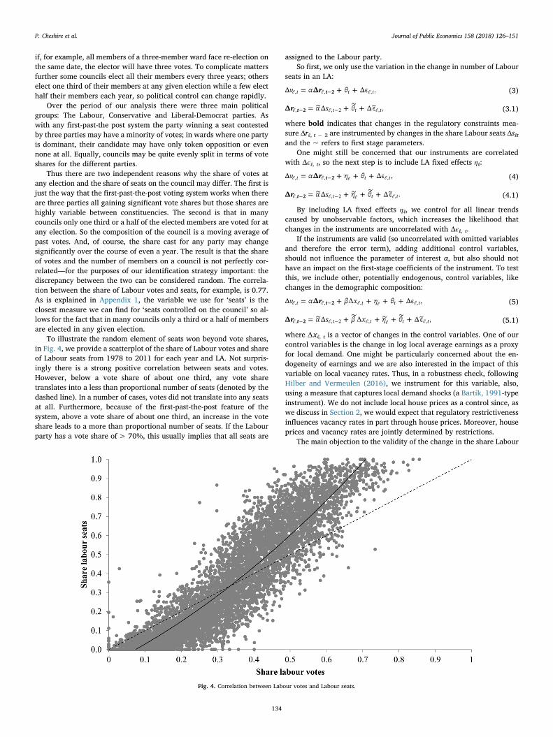
To illustrate the random element of seats won beyond vote shares,in Fig. 4, we provide a scatterplot of the share of Labour votes and shareof Labour seats from 1978 to 2011 for each year and LA. Not surpris-ingly there is a strong positive correlation between seats and votes.However, below a vote share of about one third, any vote sharetranslates into a less than proportional number of seats (denoted by thedashed line). In a number of cases, votes did not translate into any seatsat all. Furthermore, because of the first-past-the-post feature of thesystem, above a vote share of about one third, an increase in the voteshare leads to a more than proportional number of seats. If the Labourparty has a vote share of> 70%, this usually implies that all seats are

assigned to the Labour party.So first, we only use the variation in the change in number of Labour

seats in an LA:

= + +−rv α θΔΔ Δϵ ,tt t tℓ 2ℓ, , ℓ, (3)

= + +∼ ∼− −r α s θΔ Δ Δϵ~ ,t t t tℓ 2, ℓ, 2 ℓ, (3.1)

where bold indicates that changes in the regulatory constraints mea-sure Δrℓ, t − 2 are instrumented by changes in the share Labour seats Δsℓtand the ~ refers to first stage parameters.

One might still be concerned that our instruments are correlatedwith Δϵℓ, t, so the next step is to include LA fixed effects ηℓ:

= + + +−rv α η θΔΔ Δϵ ,tt t tℓ 2ℓ, , ℓ ℓ, (4)

= + + +∼ ∼∼− −r α s η θΔ Δ Δϵ~ .t t t tℓ 2, ℓ, 2 ℓ ℓ, (4.1)

By including LA fixed effects ηℓ, we control for all linear trendscaused by unobservable factors, which increases the likelihood thatchanges in the instruments are uncorrelated with Δϵℓ, t.

If the instruments are valid (so uncorrelated with omitted variablesand therefore the error term), adding additional control variables,should not influence the parameter of interest α, but also should nothave an impact on the first-stage coefficients of the instrument. To testthis, we include other, potentially endogenous, control variables, likechanges in the demographic composition:

= + ∆ + + +−rv α β x η θΔΔ Δϵ ,tt t t tℓ 2ℓ, , ℓ, ℓ ℓ, (5)

= + ∆ + + +∼ ∼∼∼− −r α s β x η θΔ Δ Δϵ~ ,t t t t tℓ 2, ℓ, 2 ℓ, ℓ ℓ, (5.1)

where Δxℓ, t is a vector of changes in the control variables. One of ourcontrol variables is the change in log local average earnings as a proxyfor local demand. One might be particularly concerned about the en-dogeneity of earnings and we are also interested in the impact of thisvariable on local vacancy rates. Thus, in a robustness check, followingHilber and Vermeulen (2016), we instrument for this variable, also,using a measure that captures local demand shocks (a Bartik, 1991-typeinstrument). We do not include local house prices as a control since, aswe discuss in Section 2, we would expect that regulatory restrictivenessinfluences vacancy rates in part through house prices. Moreover, houseprices and vacancy rates are jointly determined by restrictions.

The main objection to the validity of the change in the share Labour

Fig. 4. Correlation between Labour votes and Labour seats.

P. Cheshire et al. Journal of Public Economics 158 (2018) 126–151

134

seats-instrument is that it may be correlated with (potentially non-linear) unobserved trends. For example, some local housing markets inthe Greater London Area have experienced a substantial inflow ofwealthy residents during the last two decades, leading to changes in thedemographic composition of the local market and therefore also tochanges in voting behaviour. We thus control for a flexible function oflocal vote shares of the previous local election, identifying regulatoryrestrictiveness from the random component generated by the particularfeatures of the English local government and electoral systems dis-cussed above which ensure the seats allocated to parties are veryseldom proportional to the number of votes. So what we effectively useto identify regulatory restrictiveness is the number of seats that Labourwon (or lost) beyond their vote share. While Labour's local vote share maybe correlated with various demographic and socio-economic char-acteristics of the constituency, holding local vote shares constant, seatswon (or lost) above and beyond should be uncorrelated with the errorterm. We can express our final estimating (base) equation as:

= + ∆ + + + +−rv α β x π η θΔΔ Ω(Δ ) Δϵ ,tt t t t tℓ 2ℓ, , ℓ, ℓ, ℓ ℓ, (6)

= + ∆ + + + +∼ ∼∼∼ ∼− −r α s β x π η θΔ Δ Ω(Δ ) Δϵ~ ,t t t t t tℓ 2, ℓ, 2 ℓ, ℓ, ℓ ℓ, (6.1)

where πℓ, t is the share of Labour votes in the closest previous localelections, and

= ∑

= ∑∼

=

=

π γ π

π γ π

Ω(Δ ) Δ( ) and

Ω(Δ ) Δ( ).͠t n

Nn t

n

t nN

n tn

ℓ, 1 ℓ,

ℓ, 1 ℓ, (6.2)

Hence, Ω(∙) and ∙∼Ω( ) are Nth order polynomials of local vote shares

πℓ, t and γn and γ͠n are parameters to be estimated.Despite the fact that we identify changes in regulatory restrictive-

ness from the random component generated by the particular featuresof the English local government system, one might still be concernedthat greater Labour representation does not only affect regulatory re-strictiveness but may also affect other local variables that may sepa-rately affect local vacancy rates. That is, the exclusion restriction maybe violated. To address this crucial concern we first argue and provideevidence to support the claim that — unlike in countries with decen-tralised government structures— LAs in England, especially since 1972,have very little fiscal discretion or power other than making planningdecisions.14 Next, we show that even for those LAs — Unitary Autho-rities — that provide more local services than others, the effect of arandom increase in the local Labour representation has a very similareffect on local restrictiveness. This suggests that the relation betweenthe share of Labour seats and local restrictiveness may not be sig-nificantly biased by other local policies and services that may be cor-related with both regulatory restrictiveness and local vacancy rates.Most reassuringly, when we run a battery of placebo (first-stage) spe-cifications, in which we replace the change in local refusal rates withchanges in local expenditures — our placebo variables — we find nosignificant relationship between share Labour seats and these placebomeasures (see Section 3.5). This is in contrast to a strong and statisti-cally significant negative relationship between the random change inthe share of Labour seats and local refusal rates. Overall, these resultsprovide a strong indication that the exclusion restriction is not violatedand our identification strategy is valid.

3.3. Results for housing vacancies

We start by ignoring any potential endogeneity issues and simplyregress the vacancy rate on the refusal rate of major residential projects(Eq. (1)). From Fig. 5 we can see that the cross-sectional relationship

between the major refusal and the vacancy rates is negative. The re-gression line implies that a one standard deviation increase in refusalrates is associated with a 0.23 percentage point decrease in the vacancyrate (s.e. 0.040). This naïve correlation provides ‘common sense’ evi-dence supporting the view that vacant houses can be ‘regulated away’.However, the quantitative impact is not very large.

Table 2 reports estimates for Eqs. (2) to (6). In the cases of Eqs. (3)to (6) these are the second stage results of our IV-estimates. In column(1) we regress the change in the vacancy rate on the change in the refusalrate still ignoring potential endogeneity issues (Eq. 2). We first differ-ence controls to offset for any time invariant omitted characteristicssuch as differences in income levels across LAs. We see that evenwithout instrumenting for the refusal rate or adding control variables,the relationship between (the change in) planning restrictiveness and(the change in) the vacancy rate is no longer negative and statisticallysignificant.

However, because of the endogeneity concerns discussed above, thecoefficient on the refusal rate cannot be interpreted as a causal effect.So in column (2) we include LA fixed effects. The coefficient on thechange in the refusal rate variable now becomes positive and statisti-cally significant at the 10% level. In column (3) of Table 2 we addfurther controls as discussed in Section 3.1 above. The estimatedcoefficient for the change in the refusal rate is hardly affected, althoughit is not statistically significant at conventional levels anymore. Thecontrol variables often have a statistically significant impact on thechange in the vacancy rate with the anticipated sign. For example, areaswith an increasing share of elderly people or of council housing ex-perience an increase in the vacancy rate. Also, areas with an increasingunemployment rate, from which people may have been tending to moveaway, experience an increase in the vacancy rate. In areas with a risingshare of highly educated people, vacancies tend to decrease.

Still, however, regulatory restrictiveness is likely measured witherror (because developers may not apply in the first place in more re-strictive places). It may also be correlated with unobserved shocks.Moreover, we should address the potential reverse causality issue thathigher vacancy rates may induce policy makers to be more restrictive.We therefore instrument for the change in the refusal rate with thechange in the share of Labour seats in column (4). This specificationcorresponds to Eq. (3) above.

Kleibergen-Paap F-statistics indicate that there are no issues of weakidentification of regulatory restrictiveness. The results suggest that aone standard deviation increase in the refusal rate leads to an increasein the vacancy rate of 0.82 percentage points. As noted in the previoussubsection, one objection to the instrument is that it may be correlatedwith unobserved characteristics of the area. To control for this, we in-clude LA fixed effects in column (5) – corresponding to Eq. (4). Thecoefficient on the refusal rate hardly changes and remains statisticallysignificant at the 5% level. Column (6), corresponding to Eq. (5), in-cludes the same range of control variables as in column (3). This makesalmost no difference to the estimated coefficient of primary interest.

One might still be worried that changes in the share of Labour seatsare correlated with unobservable shocks (e.g. gentrification) that si-multaneously have an impact on voting behaviour and vacancy rates.So in column (7) we estimate our final model (6). That is, we ad-ditionally include a flexible function of changes in the share of Labourvotes in local elections, approximated by a fifth-order polynomial toisolate the impact of voting behaviour caused by any change in thedemographic and socio-economic composition of the LA from politicalpower (measured by seats). In the sensitivity checks, discussed below,we report results for different orders of polynomials. Reassuringly, theestimated effect of regulatory restrictiveness in column (7) is very si-milar to the previous specifications. The instrument is somewhat lessstrong (with a Kleibergen-Paap F-statistic of 8.2). Still, we find a posi-tive and economically meaningful effect of regulatory restrictiveness onthe vacancy rate: a one standard deviation increase in the refusal rateincreases the vacancy rate by 0.90 percentage points. Due to the

14 Perhaps surprisingly, Ferreira and Gyourko (2009) find that in the US – wheremunicipalities may be thought to have greater local discretion – whether the city mayor isa Democrat or a Republican makes little difference to a range of outcomes at the citylevel, including total expenditure or its allocation.

P. Cheshire et al. Journal of Public Economics 158 (2018) 126–151

135

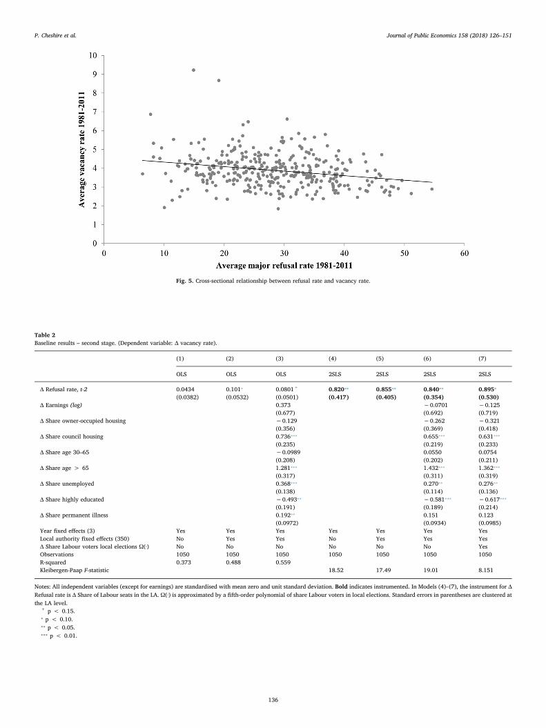
Fig. 5. Cross-sectional relationship between refusal rate and vacancy rate.

Table 2Baseline results – second stage. (Dependent variable: Δ vacancy rate).

(1) (2) (3) (4) (5) (6) (7)

OLS OLS OLS 2SLS 2SLS 2SLS 2SLS

Δ Refusal rate, t-2 0.0434 0.101⁎ 0.0801+ 0.820⁎⁎ 0.855⁎⁎ 0.840⁎⁎ 0.895⁎

(0.0382) (0.0532) (0.0501) (0.417) (0.405) (0.354) (0.530)Δ Earnings (log) 0.373 −0.0701 −0.125

(0.677) (0.692) (0.719)Δ Share owner-occupied housing −0.129 −0.262 −0.321

(0.356) (0.369) (0.418)Δ Share council housing 0.736⁎⁎⁎ 0.655⁎⁎⁎ 0.631⁎⁎⁎

(0.235) (0.219) (0.233)Δ Share age 30–65 −0.0989 0.0550 0.0754

(0.208) (0.202) (0.211)Δ Share age > 65 1.281⁎⁎⁎ 1.432⁎⁎⁎ 1.362⁎⁎⁎

(0.317) (0.311) (0.319)Δ Share unemployed 0.368⁎⁎⁎ 0.270⁎⁎ 0.276⁎⁎

(0.138) (0.114) (0.136)Δ Share highly educated −0.493⁎⁎ −0.581⁎⁎⁎ −0.617⁎⁎⁎

(0.191) (0.189) (0.214)Δ Share permanent illness 0.192⁎⁎ 0.151 0.123

(0.0972) (0.0934) (0.0985)Year fixed effects (3) Yes Yes Yes Yes Yes Yes YesLocal authority fixed effects (350) No Yes Yes No Yes Yes YesΔ Share Labour voters local elections Ω(∙) No No No No No No YesObservations 1050 1050 1050 1050 1050 1050 1050R-squared 0.373 0.488 0.559Kleibergen-Paap F-statistic 18.52 17.49 19.01 8.151

Notes: All independent variables (except for earnings) are standardised with mean zero and unit standard deviation. Bold indicates instrumented. In Models (4)–(7), the instrument for ΔRefusal rate is Δ Share of Labour seats in the LA. Ω(∙) is approximated by a fifth-order polynomial of share Labour voters in local elections. Standard errors in parentheses are clustered atthe LA level.

+ p < 0.15.⁎ p < 0.10.⁎⁎ p < 0.05.⁎⁎⁎ p < 0.01.

P. Cheshire et al. Journal of Public Economics 158 (2018) 126–151

136

correlation between changes in the Labour vote shares and changes inthe share of Labour seats, it is no surprise that the coefficient is nowonly statistically significant at the 10% level.15

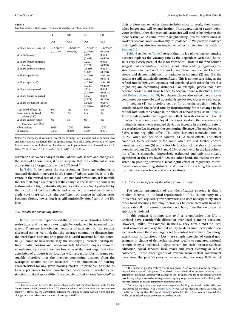
In Table 3 we report the corresponding first-stage estimates: astandard deviation increase in the share of Labour seats leads to a de-crease in the refusal rate of 0.26–0.34 standard deviations. It is notablethat the first-stage coefficients of the change in the share of Labour seatsinstrument are highly statistically significant and are hardly affected bythe inclusion of LA fixed effects and other control variables. If we in-clude vote share controls, the coefficient on change in Labour seatsbecomes slightly lower, but it is still statistically significant at the 5%level.

3.4. Results for commuting distance

In Section 2 we hypothesised that a positive relationship betweenrestrictions and vacancy rates might be explained by increased mis-match. There are few obvious measures of mismatch but for reasonsdiscussed earlier we think that the ‘average commuting distance fromthe workplace’ does not only provide a useful measure but can poten-tially illuminate in a useful way the underlying interrelationship be-tween spatial housing and Labour markets. Moreover longer commutesunambiguously signal a welfare loss. One of the most important char-acteristics of a house is its location with respect to jobs. It seems rea-sonable therefore that the average commuting distance from theworkplace should capture mismatch in this dimension of housingcharacteristics for any given housing market. In principle, householdshave a preference to live close to their workplaces. If regulatory re-strictions make it more difficult for people to find a home ‘matched’ to

their preferences on other characteristics close to work, their searchtakes longer and will extend further. This adaptation of search beha-viour implies, other things equal, vacancies will tend to be higher in themore restrictive LAs and lower in neighbouring, less restrictive ones, asworkers become more locationally mismatched.16 We provide evidencethat regulation also has an impact on other proxies for mismatch inSection 3.6.

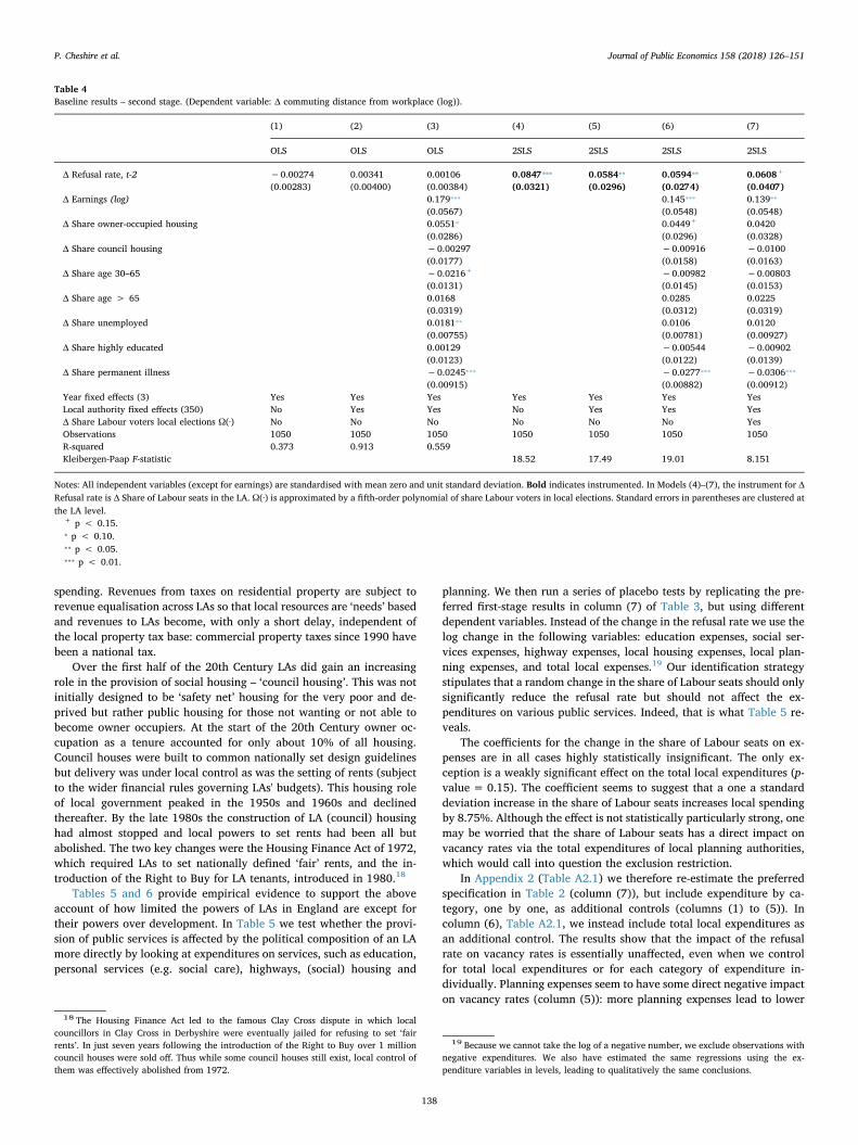
Table 4 replicates Table 2 except that the log of average commutingdistance replaces the vacancy rate as the dependent variable. The re-sults very closely parallel those for vacancies. Those in the first columnsuggest that commuting distance is not influenced by regulatory re-strictiveness in the LA of the workplace. When we include LA fixedeffects and demographic control variables in columns (2) and (3), theresults are still statistically insignificant. This is not too surprising as therefusal rate is highly endogenous and correlated with other factors thatmight explain commuting distances. For example, places that havebecome denser might have tended to become more restrictive (Hilberand Robert-Nicoud, 2013), but denser places also might have shortercommutes because jobs and households are located closer to each other.

In column (4) we therefore control for other factors that might becorrelated with the refusal rate by instrumenting for the change in therefusal rate with the change in the share of Labour seats, as in Table 2.This reveals a positive and significant effect. As restrictiveness in the LAin which a worker is employed increases so does the average com-muting distance: a one standard deviation increase in the refusal rate inthe workplace LA increases the commuting distance of its employees by8.5%, a non-negligible effect. The effect becomes somewhat smaller(5.8%) when we include in column (5) LA fixed effects. The effectcontinues to be essentially the same when we add further controlvariables in column (6) and a flexible function of the share of Labourvotes in column (7), with 5.9 and 6.1% respectively. In the last columnthe effect is somewhat imprecisely estimated and only statisticallysignificant at the 14% level.17 On the other hand, the results are con-sistent in pointing towards a meaningful effect of regulatory restric-tiveness on commuting distance, and therefore increasing the spatialmismatch between home and work locations.

3.5. Evidence in support of the identification strategy

The central assumption of our identification strategy is that arandom increase in the local representation of the Labour party onlyinfluences local regulatory restrictiveness and does not separately affectother local decisions that may themselves be correlated with local va-cancy rates. If this assumption does not hold, then the exclusion re-striction is violated.

In this context it is important to first re-emphasise that LAs inEngland have considerable discretion over local planning decisions.However, unlike, for example, in the US, they have almost no localfiscal resources and very limited ability to determine local public ser-vice levels since these are largely set by central government. To a largeextent local jurisdictions – LAs – are simply agencies of central gov-ernment in charge of delivering services locally to regulated nationalcriteria using a dedicated budget stream for each purpose (such aseducation, social services, local roads and street cleaning or refusecollection). These direct grants of revenue from central governmenthave over the past 75 years or so accounted for some 80% of LA

Table 3Baseline results – first stage. (Dependent variable: Δ refusal rate, t-2).

(1) (2) (3) (4)

OLS OLS OLS OLS

Δ Share Labour seats, t-2 −0.301*** −0.322*** −0.343*** −0.264**(0.0700) (0.0943) (0.0966) (0.114)

Δ Earnings (log) 0.579 0.504(0.461) (0.468)

Δ Share owner-occupiedhousing

0.250 0.318(0.327) (0.323)

Δ Share council housing 0.0880 0.113(0.186) (0.188)

Δ Share age 30–65 −0.194 −0.184(0.150) (0.151)

Δ Share age > 65 −0.160 −0.148(0.220) (0.218)

Δ Share unemployed 0.112 0.134(0.0880) (0.0874)

Δ Share highly educated 0.167 0.189(0.171) (0.175)

Δ Share permanent illness 0.0828 0.0673(0.0826) (0.0865)

Year fixed effects (3) Yes Yes Yes YesLocal authority fixed

effects (350)No Yes Yes Yes

Δ Share Labour voters

local elections ∙∼Ω( )

No No No Yes

Observations 1050 1050 1050 1050R-squared 0.168 0.310 0.324 0.331

Notes: All independent variables (except for earnings) are standardised with mean zeroand unit standard deviation. ∙

∼Ω( ) is approximated by a fifth-order polynomial of shareLabour voters in local elections. Standard errors in parentheses are clustered at the LAlevel. *** p < 0.01, ** p < 0.05, * p < 0.10, + p < 0.15.

15 The correlation between the share Labour votes and the share Labour seats for theCensus years is 0.88 (note that it is 0.77 when we take all available years into account, seeFigure 4). However, the correlation between the change in share Labour votes and thechange in share Labour seats is much lower (ρ= 0.481).

16 The impact of greater restrictiveness in a given LA on vacancies in the aggregate isbeyond the scope of this paper. The elasticity of substitution between housing char-acteristics (including location with respect to job) is unknown; nor is the extent to whichpeople may adopt alternative strategies to accepting longer commutes such as living withparents, friends or taking temporary accommodation.

17 One may argue that earnings are endogenous, leading to biased results. When weinstrument for earnings with a Bartik (1991)-type Labour demand shock variable, theresults are very similar. The point estimates related to the refusal rate are around 7%,while the standard errors are even somewhat lower.

P. Cheshire et al. Journal of Public Economics 158 (2018) 126–151

137

spending. Revenues from taxes on residential property are subject torevenue equalisation across LAs so that local resources are ‘needs’ basedand revenues to LAs become, with only a short delay, independent ofthe local property tax base: commercial property taxes since 1990 havebeen a national tax.

Over the first half of the 20th Century LAs did gain an increasingrole in the provision of social housing – ‘council housing’. This was notinitially designed to be ‘safety net’ housing for the very poor and de-prived but rather public housing for those not wanting or not able tobecome owner occupiers. At the start of the 20th Century owner oc-cupation as a tenure accounted for only about 10% of all housing.Council houses were built to common nationally set design guidelinesbut delivery was under local control as was the setting of rents (subjectto the wider financial rules governing LAs' budgets). This housing roleof local government peaked in the 1950s and 1960s and declinedthereafter. By the late 1980s the construction of LA (council) housinghad almost stopped and local powers to set rents had been all butabolished. The two key changes were the Housing Finance Act of 1972,which required LAs to set nationally defined ‘fair’ rents, and the in-troduction of the Right to Buy for LA tenants, introduced in 1980.18

Tables 5 and 6 provide empirical evidence to support the aboveaccount of how limited the powers of LAs in England are except fortheir powers over development. In Table 5 we test whether the provi-sion of public services is affected by the political composition of an LAmore directly by looking at expenditures on services, such as education,personal services (e.g. social care), highways, (social) housing and

planning. We then run a series of placebo tests by replicating the pre-ferred first-stage results in column (7) of Table 3, but using differentdependent variables. Instead of the change in the refusal rate we use thelog change in the following variables: education expenses, social ser-vices expenses, highway expenses, local housing expenses, local plan-ning expenses, and total local expenses.19 Our identification strategystipulates that a random change in the share of Labour seats should onlysignificantly reduce the refusal rate but should not affect the ex-penditures on various public services. Indeed, that is what Table 5 re-veals.

The coefficients for the change in the share of Labour seats on ex-penses are in all cases highly statistically insignificant. The only ex-ception is a weakly significant effect on the total local expenditures (p-value = 0.15). The coefficient seems to suggest that a one a standarddeviation increase in the share of Labour seats increases local spendingby 8.75%. Although the effect is not statistically particularly strong, onemay be worried that the share of Labour seats has a direct impact onvacancy rates via the total expenditures of local planning authorities,which would call into question the exclusion restriction.

In Appendix 2 (Table A2.1) we therefore re-estimate the preferredspecification in Table 2 (column (7)), but include expenditure by ca-tegory, one by one, as additional controls (columns (1) to (5)). Incolumn (6), Table A2.1, we instead include total local expenditures asan additional control. The results show that the impact of the refusalrate on vacancy rates is essentially unaffected, even when we controlfor total local expenditures or for each category of expenditure in-dividually. Planning expenses seem to have some direct negative impacton vacancy rates (column (5)): more planning expenses lead to lower

Table 4Baseline results – second stage. (Dependent variable: Δ commuting distance from workplace (log)).

(1) (2) (3) (4) (5) (6) (7)

OLS OLS OLS 2SLS 2SLS 2SLS 2SLS

Δ Refusal rate, t-2 −0.00274 0.00341 0.00106 0.0847⁎⁎⁎ 0.0584⁎⁎ 0.0594⁎⁎ 0.0608+

(0.00283) (0.00400) (0.00384) (0.0321) (0.0296) (0.0274) (0.0407)Δ Earnings (log) 0.179⁎⁎⁎ 0.145⁎⁎⁎ 0.139⁎⁎

(0.0567) (0.0548) (0.0548)Δ Share owner-occupied housing 0.0551⁎ 0.0449+ 0.0420

(0.0286) (0.0296) (0.0328)Δ Share council housing −0.00297 −0.00916 −0.0100

(0.0177) (0.0158) (0.0163)Δ Share age 30–65 −0.0216+ −0.00982 −0.00803

(0.0131) (0.0145) (0.0153)Δ Share age > 65 0.0168 0.0285 0.0225

(0.0319) (0.0312) (0.0319)Δ Share unemployed 0.0181⁎⁎ 0.0106 0.0120

(0.00755) (0.00781) (0.00927)Δ Share highly educated 0.00129 −0.00544 −0.00902

(0.0123) (0.0122) (0.0139)Δ Share permanent illness −0.0245⁎⁎⁎ −0.0277⁎⁎⁎ −0.0306⁎⁎⁎

(0.00915) (0.00882) (0.00912)Year fixed effects (3) Yes Yes Yes Yes Yes Yes YesLocal authority fixed effects (350) No Yes Yes No Yes Yes YesΔ Share Labour voters local elections Ω(∙) No No No No No No YesObservations 1050 1050 1050 1050 1050 1050 1050R-squared 0.373 0.913 0.559Kleibergen-Paap F-statistic 18.52 17.49 19.01 8.151

Notes: All independent variables (except for earnings) are standardised with mean zero and unit standard deviation. Bold indicates instrumented. In Models (4)–(7), the instrument for ΔRefusal rate is Δ Share of Labour seats in the LA. Ω(∙) is approximated by a fifth-order polynomial of share Labour voters in local elections. Standard errors in parentheses are clustered atthe LA level.

+ p < 0.15.⁎ p < 0.10.⁎⁎ p < 0.05.⁎⁎⁎ p < 0.01.

18 The Housing Finance Act led to the famous Clay Cross dispute in which localcouncillors in Clay Cross in Derbyshire were eventually jailed for refusing to set ‘fairrents’. In just seven years following the introduction of the Right to Buy over 1 millioncouncil houses were sold off. Thus while some council houses still exist, local control ofthem was effectively abolished from 1972.

19 Because we cannot take the log of a negative number, we exclude observations withnegative expenditures. We also have estimated the same regressions using the ex-penditure variables in levels, leading to qualitatively the same conclusions.

P. Cheshire et al. Journal of Public Economics 158 (2018) 126–151

138

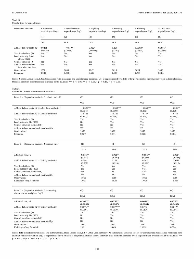
Table 5Placebo tests for expenditures.

Dependent variable: Δ Educationexpenditures (log)

Δ Social servicesexpenditures (log)

Δ Highwayexpenditures (log)

Δ Housingexpenditures (log)

Δ Planningexpenditures (log)

Δ Total localexpenditures (log)

(1) (2) (3) (4) (5) (6)

OLS OLS OLS OLS OLS OLS

Δ Share Labour seats, t-2 0.0231 −0.0107 0.0224 0.126 0.00629 0.0875+

(0.0550) (0.0165) (0.0321) (0.110) (0.0871) (0.0559)Year fixed effects (3) Yes Yes Yes Yes Yes YesLocal authority fixed

effects (350)Yes Yes Yes Yes Yes Yes

Control variables (8) Yes Yes Yes Yes Yes YesΔ Share Labour voters

local elections Ω(∙)Yes Yes Yes Yes Yes Yes

Observations 1050 1050 1047 1014 1024 1050R-squared 0.082 0.583 0.529 0.661 0.431 0.326

Notes: Δ Share Labour seats, t-2 is standardised with mean zero and unit standard deviation. Ω(∙) is approximated by a fifth-order polynomial of share Labour voters in local elections.Standard errors in parentheses are clustered at the LA level. *** p < 0.01, ** p < 0.05, * p < 0.10, + p < 0.15.

Table 6Results for Unitary Authorities and other LAs.

Panel A – (Dependent variable: Δ refusal rate, t-2) (1) (2) (3) (4)

OLS OLS OLS OLS

Δ Share Labour seats, t-2× other local authority −0.326*** −0.352*** −0.365*** −0.291**(0.0743) (0.0998) (0.102) (0.120)

Δ Share Labour seats, t-2× Unitary authority −0.144 −0.121 −0.187 −0.153(0.162) (0.210) (0.205) (0.215)

Year fixed effects (3) Yes Yes Yes YesLocal authority FEs (350) No Yes Yes YesControl variables included (8) No No Yes Yes

Δ Share Labour voters local elections ∙∼Ω( ) No No No Yes

Observations 1050 1050 1050 1050R-squared 0.169 0.311 0.325 0.326

Panel B – (Dependent variable: Δ vacancy rate) (1) (2) (3) (4)

2SLS 2SLS 2SLS 2SLS

Δ Refusal rate, t-2 0.915** 0.906** 0.855** 0.935*(0.423) (0.399) (0.359) (0.541)

Δ Share Labour seats, t-2× Unitary authority 0.209 0.126 0.0421 0.0786(0.207) (0.216) (0.196) (0.212)

Year fixed effects (3) Yes Yes Yes YesLocal authority FEs (350) No Yes Yes YesControl variables included (8) No No Yes Yes

Δ Share Labour voters local elections ∙∼Ω( ) No No No Yes

Observations 1050 1050 1050 1050Kleibergen-Paap F-statistic 19.31 18.65 19.25 8.354

Panel C – (Dependent variable: Δ commutingdistance from workplace (log))

(1) (2) (3) (4)

2SLS 2SLS 2SLS 2SLS

Δ Refusal rate, t-2 0.102*** 0.0735** 0.0664** 0.0720*(0.0342) (0.0307) (0.0284) (0.0432)

Δ Share Labour seats, t-2× Unitary authority 0.0371** 0.0377*** 0.0195 0.0217+

(0.0164) (0.0139) (0.0136) (0.0141)Year fixed effects (3) Yes Yes Yes YesLocal authority FEs (350) No Yes Yes YesControl variables included (8) No No Yes Yes

Δ Share Labour voters local elections ∙∼Ω( ) No No No Yes

Observations 1050 1050 1050 1050Kleibergen-Paap F-statistic 19.31 18.65 19.25 8.354

Notes: Bold indicates instrumented. The instrument is Δ Share Labour seats, t-2×Other Local authority. All independent variables (except for earnings) are standardised with mean zeroand unit standard deviation. Ω (∙) is approximated by a fifth-order polynomial of share Labour voters in local elections. Standard errors in parentheses are clustered at the LA level. ***p < 0.01, ** p < 0.05, * p < 0.10, + p < 0.15.

P. Cheshire et al. Journal of Public Economics 158 (2018) 126–151

139

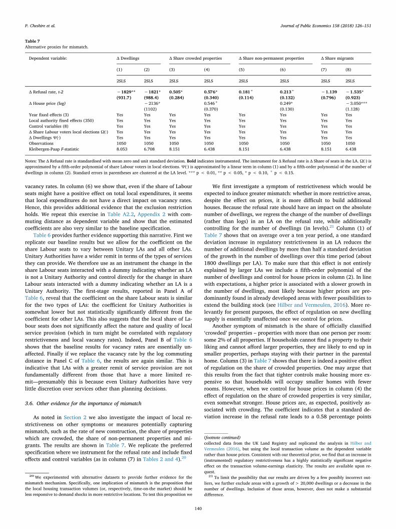
vacancy rates. In column (6) we show that, even if the share of Labourseats might have a positive effect on total local expenditures, it seemsthat local expenditures do not have a direct impact on vacancy rates.Hence, this provides additional evidence that the exclusion restrictionholds. We repeat this exercise in Table A2.2, Appendix 2 with com-muting distance as dependent variable and show that the estimatedcoefficients are also very similar to the baseline specification.

Table 6 provides further evidence supporting this narrative. First wereplicate our baseline results but we allow for the coefficient on theshare Labour seats to vary between Unitary LAs and all other LAs.Unitary Authorities have a wider remit in terms of the types of servicesthey can provide. We therefore use as an instrument the change in theshare Labour seats interacted with a dummy indicating whether an LAis not a Unitary Authority and control directly for the change in shareLabour seats interacted with a dummy indicating whether an LA is aUnitary Authority. The first-stage results, reported in Panel A ofTable 6, reveal that the coefficient on the share Labour seats is similarfor the two types of LAs: the coefficient for Unitary Authorities issomewhat lower but not statistically significantly different from thecoefficient for other LAs. This also suggests that the local share of La-bour seats does not significantly affect the nature and quality of localservice provision (which in turn might be correlated with regulatoryrestrictiveness and local vacancy rates). Indeed, Panel B of Table 6shows that the baseline results for vacancy rates are essentially un-affected. Finally if we replace the vacancy rate by the log commutingdistance in Panel C of Table 6, the results are again similar. This isindicative that LAs with a greater remit of service provision are notfundamentally different from those that have a more limited re-mit—presumably this is because even Unitary Authorities have verylittle discretion over services other than planning decisions.

3.6. Other evidence for the importance of mismatch

As noted in Section 2 we also investigate the impact of local re-strictiveness on other symptoms or measures potentially capturingmismatch, such as the rate of new construction, the share of propertieswhich are crowded, the share of non-permanent properties and mi-grants. The results are shown in Table 7. We replicate the preferredspecification where we instrument for the refusal rate and include fixedeffects and control variables (as in column (7) in Tables 2 and 4).20

We first investigate a symptom of restrictiveness which would beexpected to induce greater mismatch: whether in more restrictive areas,despite the effect on prices, it is more difficult to build additionalhouses. Because the refusal rate should have an impact on the absolutenumber of dwellings, we regress the change of the number of dwellings(rather than logs) in an LA on the refusal rate, while additionallycontrolling for the number of dwellings (in levels).21 Column (1) ofTable 7 shows that on average over a ten year period, a one standarddeviation increase in regulatory restrictiveness in an LA reduces thenumber of additional dwellings by more than half a standard deviationof the growth in the number of dwellings over this time period (about1800 dwellings per LA). To make sure that this effect is not entirelyexplained by larger LAs we include a fifth-order polynomial of thenumber of dwellings and control for house prices in column (2). In linewith expectations, a higher price is associated with a slower growth inthe number of dwellings, most likely because higher prices are pre-dominantly found in already developed areas with fewer possibilities toextend the building stock (see Hilber and Vermeulen, 2016). More re-levantly for present purposes, the effect of regulation on new dwellingsupply is essentially unaffected once we control for prices.

Another symptom of mismatch is the share of officially classified‘crowded’ properties – properties with more than one person per room:some 2% of all properties. If households cannot find a property to theirliking and cannot afford larger properties, they are likely to end up insmaller properties, perhaps staying with their partner in the parentalhome. Column (3) in Table 7 shows that there is indeed a positive effectof regulation on the share of crowded properties. One may argue thatthis results from the fact that tighter controls make housing more ex-pensive so that households will occupy smaller homes with fewerrooms. However, when we control for house prices in column (4) theeffect of regulation on the share of crowded properties is very similar,even somewhat stronger. House prices are, as expected, positively as-sociated with crowding. The coefficient indicates that a standard de-viation increase in the refusal rate leads to a 0.58 percentage points

Table 7Alternative proxies for mismatch.

Dependent variable: Δ Dwellings Δ Share crowded properties Δ Share non-permanent properties Δ Share migrants

(1) (2) (3) (4) (5) (6) (7) (8)

2SLS 2SLS 2SLS 2SLS 2SLS 2SLS 2SLS 2SLS

Δ Refusal rate, t-2 −1829** −1821* 0.505* 0.576* 0.181+ 0.213+ −1.139 −1.535*(931.7) (988.4) (0.284) (0.340) (0.114) (0.132) (0.796) (0.923)

Δ House price (log) −2136* 0.546+ 0.249* −3.050***(1102) (0.370) (0.130) (1.128)

Year fixed effects (3) Yes Yes Yes Yes Yes Yes Yes YesLocal authority fixed effects (350) Yes Yes Yes Yes Yes Yes Yes YesControl variables (8) Yes Yes Yes Yes Yes Yes Yes YesΔ Share Labour voters local elections Ω(∙) Yes Yes Yes Yes Yes Yes Yes YesΔ Dwellings Ψ(∙) Yes Yes Yes Yes Yes Yes Yes YesObservations 1050 1050 1050 1050 1050 1050 1050 1050Kleibergen-Paap F-statistic 8.053 6.708 8.151 6.438 8.151 6.438 8.151 6.438

Notes: The Δ Refusal rate is standardised with mean zero and unit standard deviation. Bold indicates instrumented. The instrument for Δ Refusal rate is Δ Share of seats in the LA. Ω(∙) isapproximated by a fifth-order polynomial of share Labour voters in local elections. Ψ(∙) is approximated by a linear term in column (1) and by a fifth-order polynomial of the number ofdwellings in column (2). Standard errors in parentheses are clustered at the LA level. *** p < 0.01, ** p < 0.05, * p < 0.10, + p < 0.15.

20 We experimented with alternative datasets to provide further evidence for themismatch mechanism. Specifically, one implication of mismatch is the proposition thatthe local housing transaction volumes (or, respectively, time-on-the market) should beless responsive to demand shocks in more restrictive locations. To test this proposition we

(footnote continued)collected data from the UK Land Registry and replicated the analysis in Hilber andVermeulen (2016), but using the local transaction volume as the dependent variablerather than house prices. Consistent with our theoretical prior, we find that an increase in(instrumented) regulatory restrictiveness has a highly statistically significant negativeeffect on the transaction volume-earnings elasticity. The results are available upon re-quest.

21 To limit the possibility that our results are driven by a few possibly incorrect out-liers, we further exclude areas with a growth of> 20,000 dwellings or a decrease in thenumber of dwellings. Inclusion of those areas, however, does not make a substantialdifference.

P. Cheshire et al. Journal of Public Economics 158 (2018) 126–151

140

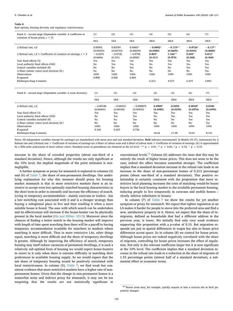
increase in the share of crowded properties (about one-third of astandard deviation). Hence, although the results are only significant atthe 10% level, the implied magnitude of the point estimates is non-negligible.

A further symptom or proxy for mismatch is explored in columns (5)and (6) of Table 7, the share of non-permanent dwellings. Our under-lying explanation for why this measure should proxy for housingmarket mismatch is that in more restrictive markets there is an in-centive to accept even less optimally matched housing characteristics inthe short term in order to intensify and increase the efficiency of search.Living in temporary accommodation – mainly caravans or trailers - hasa low switching cost associated with it and is a cheaper strategy thanbuying a suboptimal place to live and then reselling it when a moresuitable house is found. The ease with which search can be undertakenand its effectiveness will increase if the house-hunter can be physicallypresent in the local market (Ha and Hilber, 2013). Moreover since thechances of finding a better match in the housing market will improvewith length of time spent searching then there will be a payoff to havingtemporary accommodation available for searchers in markets wherematching is more difficult. Thus in more restrictive LAs, other thingsequal, matching is more difficult and the share of temporary dwellingsis greater. Although by improving the efficiency of search, temporaryhousing may itself reduce vacancies of permanent dwellings, it is such arelatively sub-optimal form of housing we would expect house-huntersto resort to it only when there is extreme difficulty in matching theirpreferences to available housing supply. So we would expect that thenet share of temporary housing would be positively correlated withlocal restrictiveness. In column (5), Table 7, we find weak but con-sistent evidence that more restrictive markets have a higher rate of non-permanent homes. Given that the change in non-permanent homes is asomewhat noisy and indirect proxy for mismatch, it may not be toosurprising that the results are not statistically significant at

conventional levels.22 Column (6) addresses the issue that this may beentirely the result of higher house prices. This does not seem to be thecase; indeed the effect becomes somewhat stronger. The coefficientimplies that a standard deviation increase in the refusal rate leads to anincrease in the share of non-permanent homes of 0.213 percentagepoints (about one-third of a standard deviation). This positive re-lationship is certainly consistent with the proposition that more re-strictive local planning increases the costs of matching would-be housebuyers in the local housing market to the available permanent housing,inducing people to live temporarily in caravans and mobile homes –clearly inferior substitutes to houses.

In column (7) of Table 7 we show the results for yet anothersymptom or proxy for mismatch. We expect that tighter regulation in anLA makes it harder for people to move into the preferred area and find anew, satisfactory property in it. Hence, we expect that the share of in-migrants, defined as households that had a different address in theprevious year, is lower. We initially find only very weak evidencesupporting this proposition with a p-value of 0.15. But migration re-sponds not just to spatial differences in wages but also to house pricedifferences across space. So in column (8) we control for house prices.Although house prices are indeed negatively correlated with the shareof migrants, controlling for house prices increases the effect of regula-tion. Not only is the relevant coefficient larger but it is now significantat the 10% level. The coefficient implies that a standard deviation in-crease in the refusal rate leads to a reduction in the share of migrants of1.53 percentage points (almost half of a standard deviation), a sub-stantial effect in economic terms.

Table 8Real options, housing diversity and regulatory restrictiveness.

Panel A – second stage (Dependent variable: Δ coefficient ofvariation of house prices, t + 3)

(1) (2) (3) (4) (5) (6) (7)

OLS OLS OLS 2SLS 2SLS 2SLS 2SLS

Δ Refusal rate, t-2 0.00501 0.00784 0.00857 −0.0892* −0.119** −0.0726* −0.117*(0.00453) (0.00743) (0.00659) (0.0480) (0.0605) (0.0434) (0.0680)

Δ Refusal rate, t-2× Coefficient of variation of earnings, t + 3 −0.0375 −0.0725 −0.0758 0.804* 1.166** 0.693* 0.812*(0.0606) (0.101) (0.0858) (0.411) (0.570) (0.368) (0.468)

Year fixed effects (3) Yes Yes Yes Yes Yes Yes YesLocal authority fixed effects (350) No Yes Yes No Yes Yes YesControl variables included (8) No No Yes No No Yes YesΔ Share Labour voters local elections Ω(∙) No No No No No No YesObservations 1050 1050 1050 1050 1050 1050 1050R-squared 0.808 0.826 0.864Kleibergen-Paap F-statistic 5.212 4.573 5.419 2.893

Panel B – second stage (Dependent variable: Δ room diversity) (1) (2) (3) (4) (5) (6) (7)

OLS OLS OLS 2SLS 2SLS 2SLS 2SLS

Δ Refusal rate, t-2 −0.00186 −0.00410 −0.000875 0.0900* 0.0294 0.00427 0.0180(0.00465) (0.00549) (0.00492) (0.0485) (0.0339) (0.0276) (0.0399)

Year fixed effects (3) Yes Yes Yes Yes Yes Yes YesLocal authority fixed effects (350) No Yes Yes No Yes Yes YesControl variables included (8) No No Yes No No Yes YesΔ Share Labour voters local elections Ω(∙) No No No No No No YesObservations 1050 1050 1050 1050 1050 1050 1050R-squared 0.160 0.653 0.726Kleibergen-Paap F-statistic 18.52 17.49 19.01 8.151

Notes: All independent variables (except for earnings) are standardised with mean zero and unit standard deviation. Bold indicates instrumented. In Models (4)–(7), instruments for ΔRefusal rate and Δ Refusal rate × Coefficient of variation of earnings are Δ Share of Labour seats and Δ Share of Labour seats × Coefficient of variation of earnings. Ω(∙) is approximatedby a fifth-order polynomial of share Labour voters. Standard errors in parentheses are clustered at the LA level. *** p < 0.01, ** p < 0.05, * p < 0.10, + p < 0.15.

22 Resort areas may, for example, quickly acquire or lose a caravan site as their po-pularity changes.

P. Cheshire et al. Journal of Public Economics 158 (2018) 126–151

141

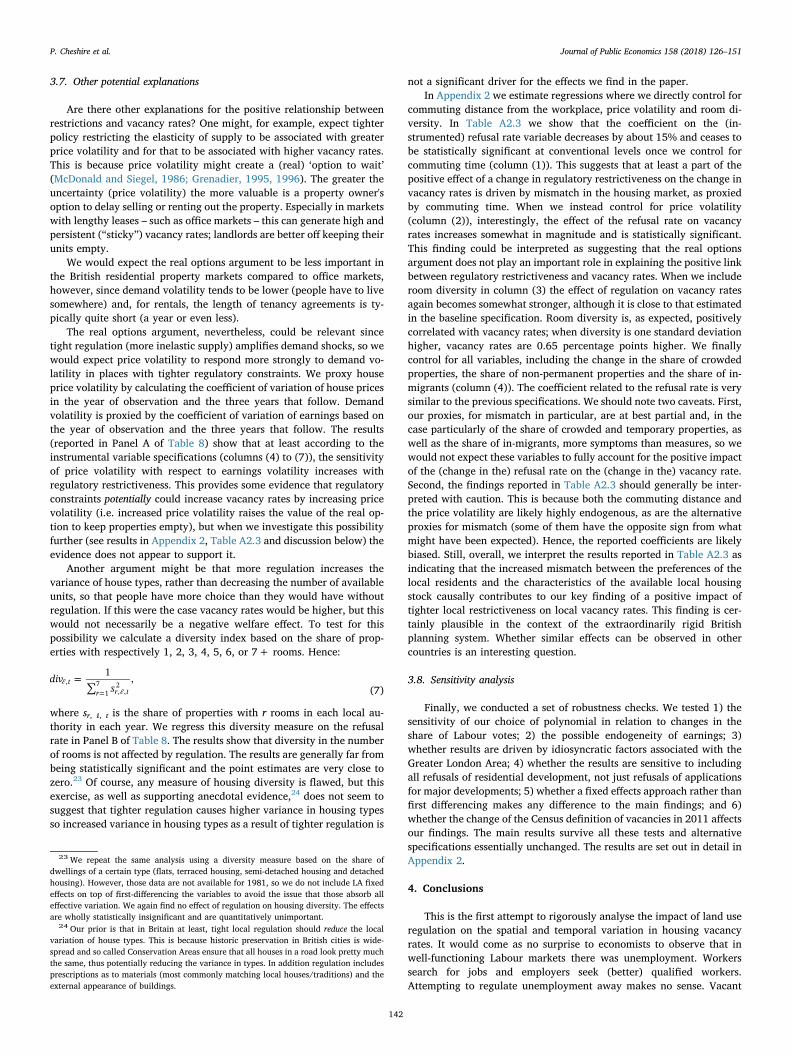
3.7. Other potential explanations

Are there other explanations for the positive relationship betweenrestrictions and vacancy rates? One might, for example, expect tighterpolicy restricting the elasticity of supply to be associated with greaterprice volatility and for that to be associated with higher vacancy rates.This is because price volatility might create a (real) ‘option to wait’(McDonald and Siegel, 1986; Grenadier, 1995, 1996). The greater theuncertainty (price volatility) the more valuable is a property owner'soption to delay selling or renting out the property. Especially in marketswith lengthy leases – such as office markets – this can generate high andpersistent (“sticky”) vacancy rates; landlords are better off keeping theirunits empty.

We would expect the real options argument to be less important inthe British residential property markets compared to office markets,however, since demand volatility tends to be lower (people have to livesomewhere) and, for rentals, the length of tenancy agreements is ty-pically quite short (a year or even less).

The real options argument, nevertheless, could be relevant sincetight regulation (more inelastic supply) amplifies demand shocks, so wewould expect price volatility to respond more strongly to demand vo-latility in places with tighter regulatory constraints. We proxy houseprice volatility by calculating the coefficient of variation of house pricesin the year of observation and the three years that follow. Demandvolatility is proxied by the coefficient of variation of earnings based onthe year of observation and the three years that follow. The results(reported in Panel A of Table 8) show that at least according to theinstrumental variable specifications (columns (4) to (7)), the sensitivityof price volatility with respect to earnings volatility increases withregulatory restrictiveness. This provides some evidence that regulatoryconstraints potentially could increase vacancy rates by increasing pricevolatility (i.e. increased price volatility raises the value of the real op-tion to keep properties empty), but when we investigate this possibilityfurther (see results in Appendix 2, Table A2.3 and discussion below) theevidence does not appear to support it.

Another argument might be that more regulation increases thevariance of house types, rather than decreasing the number of availableunits, so that people have more choice than they would have withoutregulation. If this were the case vacancy rates would be higher, but thiswould not necessarily be a negative welfare effect. To test for thispossibility we calculate a diversity index based on the share of prop-erties with respectively 1, 2, 3, 4, 5, 6, or 7+ rooms. Hence:

=∑ =

divs

1 ,tr r t

ℓ,1

7,ℓ,

2 (7)

where sr, ℓ, t is the share of properties with r rooms in each local au-thority in each year. We regress this diversity measure on the refusalrate in Panel B of Table 8. The results show that diversity in the numberof rooms is not affected by regulation. The results are generally far frombeing statistically significant and the point estimates are very close tozero.23 Of course, any measure of housing diversity is flawed, but thisexercise, as well as supporting anecdotal evidence,24 does not seem tosuggest that tighter regulation causes higher variance in housing typesso increased variance in housing types as a result of tighter regulation is

not a significant driver for the effects we find in the paper.In Appendix 2 we estimate regressions where we directly control for

commuting distance from the workplace, price volatility and room di-versity. In Table A2.3 we show that the coefficient on the (in-strumented) refusal rate variable decreases by about 15% and ceases tobe statistically significant at conventional levels once we control forcommuting time (column (1)). This suggests that at least a part of thepositive effect of a change in regulatory restrictiveness on the change invacancy rates is driven by mismatch in the housing market, as proxiedby commuting time. When we instead control for price volatility(column (2)), interestingly, the effect of the refusal rate on vacancyrates increases somewhat in magnitude and is statistically significant.This finding could be interpreted as suggesting that the real optionsargument does not play an important role in explaining the positive linkbetween regulatory restrictiveness and vacancy rates. When we includeroom diversity in column (3) the effect of regulation on vacancy ratesagain becomes somewhat stronger, although it is close to that estimatedin the baseline specification. Room diversity is, as expected, positivelycorrelated with vacancy rates; when diversity is one standard deviationhigher, vacancy rates are 0.65 percentage points higher. We finallycontrol for all variables, including the change in the share of crowdedproperties, the share of non-permanent properties and the share of in-migrants (column (4)). The coefficient related to the refusal rate is verysimilar to the previous specifications. We should note two caveats. First,our proxies, for mismatch in particular, are at best partial and, in thecase particularly of the share of crowded and temporary properties, aswell as the share of in-migrants, more symptoms than measures, so wewould not expect these variables to fully account for the positive impactof the (change in the) refusal rate on the (change in the) vacancy rate.Second, the findings reported in Table A2.3 should generally be inter-preted with caution. This is because both the commuting distance andthe price volatility are likely highly endogenous, as are the alternativeproxies for mismatch (some of them have the opposite sign from whatmight have been expected). Hence, the reported coefficients are likelybiased. Still, overall, we interpret the results reported in Table A2.3 asindicating that the increased mismatch between the preferences of thelocal residents and the characteristics of the available local housingstock causally contributes to our key finding of a positive impact oftighter local restrictiveness on local vacancy rates. This finding is cer-tainly plausible in the context of the extraordinarily rigid Britishplanning system. Whether similar effects can be observed in othercountries is an interesting question.

3.8. Sensitivity analysis

Finally, we conducted a set of robustness checks. We tested 1) thesensitivity of our choice of polynomial in relation to changes in theshare of Labour votes; 2) the possible endogeneity of earnings; 3)whether results are driven by idiosyncratic factors associated with theGreater London Area; 4) whether the results are sensitive to includingall refusals of residential development, not just refusals of applicationsfor major developments; 5) whether a fixed effects approach rather thanfirst differencing makes any difference to the main findings; and 6)whether the change of the Census definition of vacancies in 2011 affectsour findings. The main results survive all these tests and alternativespecifications essentially unchanged. The results are set out in detail inAppendix 2.

4. Conclusions

This is the first attempt to rigorously analyse the impact of land useregulation on the spatial and temporal variation in housing vacancyrates. It would come as no surprise to economists to observe that inwell-functioning Labour markets there was unemployment. Workerssearch for jobs and employers seek (better) qualified workers.Attempting to regulate unemployment away makes no sense. Vacant

23 We repeat the same analysis using a diversity measure based on the share ofdwellings of a certain type (flats, terraced housing, semi-detached housing and detachedhousing). However, those data are not available for 1981, so we do not include LA fixedeffects on top of first-differencing the variables to avoid the issue that those absorb alleffective variation. We again find no effect of regulation on housing diversity. The effectsare wholly statistically insignificant and are quantitatively unimportant.

24 Our prior is that in Britain at least, tight local regulation should reduce the localvariation of house types. This is because historic preservation in British cities is wide-spread and so called Conservation Areas ensure that all houses in a road look pretty muchthe same, thus potentially reducing the variance in types. In addition regulation includesprescriptions as to materials (most commonly matching local houses/traditions) and theexternal appearance of buildings.

P. Cheshire et al. Journal of Public Economics 158 (2018) 126–151

142

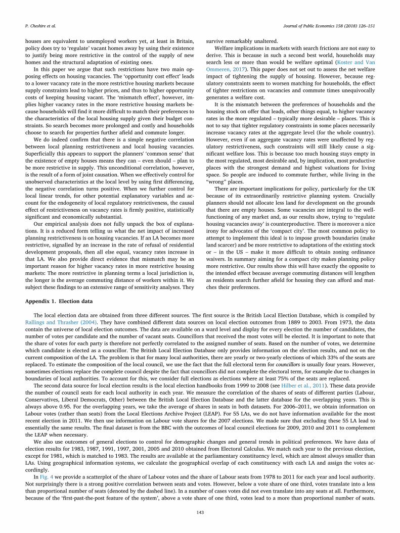
houses are equivalent to unemployed workers yet, at least in Britain,policy does try to ‘regulate’ vacant homes away by using their existenceto justify being more restrictive in the control of the supply of newhomes and the structural adaptation of existing ones.

In this paper we argue that such restrictions have two main op-posing effects on housing vacancies. The ‘opportunity cost effect’ leadsto a lower vacancy rate in the more restrictive housing markets becausesupply constraints lead to higher prices, and thus to higher opportunitycosts of keeping housing vacant. The ‘mismatch effect’, however, im-plies higher vacancy rates in the more restrictive housing markets be-cause households will find it more difficult to match their preferences tothe characteristics of the local housing supply given their budget con-straints. So search becomes more prolonged and costly and householdschoose to search for properties further afield and commute longer.

We do indeed confirm that there is a simple negative correlationbetween local planning restrictiveness and local housing vacancies.Superficially this appears to support the planners' ‘common sense’ thatthe existence of empty houses means they can – even should – plan tobe more restrictive in supply. This unconditional correlation, however,is the result of a form of joint causation. When we effectively control forunobserved characteristics at the local level by using first differencing,the negative correlation turns positive. When we further control forlocal linear trends, for other potential explanatory variables and ac-count for the endogeneity of local regulatory restrictiveness, the causaleffect of restrictiveness on vacancy rates is firmly positive, statisticallysignificant and economically substantial.

Our empirical analysis does not fully unpack the box of explana-tions. It is a reduced form telling us what the net impact of increasedplanning restrictiveness is on housing vacancies. If an LA becomes morerestrictive, signalled by an increase in the rate of refusal of residentialdevelopment proposals, then all else equal, vacancy rates increase inthat LA. We also provide direct evidence that mismatch may be animportant reason for higher vacancy rates in more restrictive housingmarkets: The more restrictive in planning terms a local jurisdiction is,the longer is the average commuting distance of workers within it. Wesubject these findings to an extensive range of sensitivity analyses. They

survive remarkably unaltered.Welfare implications in markets with search frictions are not easy to

derive. This is because in such a second best world, households maysearch less or more than would be welfare optimal (Koster and VanOmmeren, 2017). This paper does not set out to assess the net welfareimpact of tightening the supply of housing. However, because reg-ulatory constraints seem to worsen matching for households, the effectof tighter restrictions on vacancies and commute times unequivocallygenerates a welfare cost.

It is the mismatch between the preferences of households and thehousing stock on offer that leads, other things equal, to higher vacancyrates in the more regulated – typically more desirable – places. This isnot to say that tighter regulatory constraints in some places necessarilyincrease vacancy rates at the aggregate level (for the whole country).However, even if on aggregate vacancy rates were unaffected by reg-ulatory restrictiveness, such constraints will still likely cause a sig-nificant welfare loss. This is because too much housing stays empty inthe most regulated, most desirable and, by implication, most productiveplaces with the strongest demand and highest valuations for livingspace. So people are induced to commute further, while living in the“wrong” places.

There are important implications for policy, particularly for the UKbecause of its extraordinarily restrictive planning system. Cruciallyplanners should not allocate less land for development on the groundsthat there are empty houses. Some vacancies are integral to the well-functioning of any market and, as our results show, trying to ‘regulatehousing vacancies away’ is counterproductive. There is moreover a niceirony for advocates of the ‘compact city’. The most common policy toattempt to implement this ideal is to impose growth boundaries (makeland scarcer) and be more restrictive to adaptations of the existing stockor – in the US – make it more difficult to obtain zoning ordinancewaivers. In summary aiming for a compact city makes planning policymore restrictive. Our results show this will have exactly the opposite tothe intended effect because average commuting distances will lengthenas residents search further afield for housing they can afford and mat-ches their preferences.

Appendix 1. Election data

The local election data are obtained from three different sources. The first source is the British Local Election Database, which is compiled byRallings and Thrasher (2004). They have combined different data sources on local election outcomes from 1889 to 2003. From 1973, the datacontain the universe of local election outcomes. The data are available on a ward level and display for every election the number of candidates, thenumber of votes per candidate and the number of vacant seats. Councillors that received the most votes will be elected. It is important to note thatthe share of votes for each party is therefore not perfectly correlated to the assigned number of seats. Based on the number of votes, we determinewhich candidate is elected as a councillor. The British Local Election Database only provides information on the election results, and not on thecurrent composition of the LA. The problem is that for many local authorities, there are yearly or two-yearly elections of which 33% of the seats arereplaced. To estimate the composition of the local council, we use the fact that the full electoral term for councillors is usually four years. However,sometimes elections replace the complete council despite the fact that councillors did not complete the electoral term, for example due to changes inboundaries of local authorities. To account for this, we consider full elections as elections where at least 75% of the seats are replaced.

The second data source for local election results is the local election handbooks from 1999 to 2008 (see Hilber et al., 2011). These data providethe number of council seats for each local authority in each year. We measure the correlation of the shares of seats of different parties (Labour,Conservatives, Liberal Democrats, Other) between the British Local Election Database and the latter database for the overlapping years. This isalways above 0.95. For the overlapping years, we take the average of shares in seats in both datasets. For 2006–2011, we obtain information onLabour votes (rather than seats) from the Local Elections Archive Project (LEAP). For 55 LAs, we do not have information available for the mostrecent election in 2011. We then use information on Labour vote shares for the 2007 elections. We made sure that excluding these 55 LA lead toessentially the same results. The final dataset is from the BBC with the outcomes of local council elections for 2009, 2010 and 2011 to complementthe LEAP when necessary.

We also use outcomes of general elections to control for demographic changes and general trends in political preferences. We have data ofelection results for 1983, 1987, 1991, 1997, 2001, 2005 and 2010 obtained from Electoral Calculus. We match each year to the previous election,except for 1981, which is matched to 1983. The results are available at the parliamentary constituency level, which are almost always smaller thanLAs. Using geographical information systems, we calculate the geographical overlap of each constituency with each LA and assign the votes ac-cordingly.

In Fig. 4 we provide a scatterplot of the share of Labour votes and the share of Labour seats from 1978 to 2011 for each year and local authority.Not surprisingly there is a strong positive correlation between seats and votes. However, below a vote share of one third, votes translate into a lessthan proportional number of seats (denoted by the dashed line). In a number of cases votes did not even translate into any seats at all. Furthermore,because of the ‘first-past-the-post feature of the system’, above a vote share of one third, votes lead to a more than proportional number of seats.

P. Cheshire et al. Journal of Public Economics 158 (2018) 126–151

143

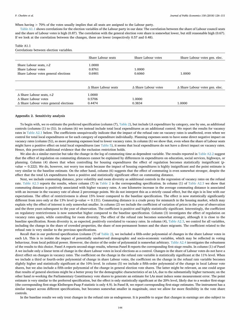
When having> 70% of the votes usually implies that all seats are assigned to the Labour party.Table A1.1 shows correlations for the election variables of the Labour party in our data: The correlation between the share of Labour council seats

and the share of Labour votes is high (0.87). The correlation with the general election vote share is somewhat lower, but still reasonable high (0.67).If we look at the correlation between the changes, these are lower (respectively 0.57 and 0.48).

Table A1.1Correlations between election variables.

Share Labour seats Share Labour votes Share Labour votes gen. elec.

Share Labour seats, t-2 1.0000Share Labour votes 0.8761 1.0000Share Labour votes general elections 0.6901 0.6060 1.0000

Δ Share Labour seats Δ Share Labour votes Δ Share Labour votes gen. elec.

Δ Share Labour seats, t-2 1.0000Δ Share Labour votes 0.5706 1.0000Δ Share Labour votes general elections 0.4474 0.3834 1.0000

Appendix 2. Sensitivity analysis

To begin with, we re-estimate the preferred specification (column (7), Table 2), but include LA expenditure by category, one by one, as additionalcontrols (columns (1) to (5)). In column (6) we instead include total local expenditures as an additional control. We report the results for vacancyrates in Table A2.1 below. The coefficients unequivocally indicate that the impact of the refusal rate on vacancy rates is unaffected, even when wecontrol for total local expenditures or for each category of expenditure individually. Planning expenses seem to have some direct negative impact onvacancy rates (column (5)), so more planning expenses lead to lower vacancy rates. In column (6) we show that, even when the share of Labour seatsmight have a positive effect on total local expenditures (see Table 5), it seems that local expenditures do not have a direct impact on vacancy rates.Hence, this provides additional evidence that the exclusion restriction holds.

We also do a similar exercise but take the change in the log of commuting time as dependent variable. The results reported in Table A2.2 suggestthat the effect of regulation on commuting distances cannot be explained by differences in expenditures on education, social services, highways, orplanning. Column (4) shows that when controlling for housing expenditures the effect of regulation becomes statistically insignificant (p-value = 0.222). We do, however, not worry too much because the impact of housing expenditures is highly insignificant and the point estimate isvery similar to the baseline estimate. On the other hand, column (6) suggests that the effect of commuting is even somewhat stronger, despite theeffect that the total LA expenditures have a positive and statistically significant effect on commuting distance.

Next, we include commuting distance, price volatility and room diversity as additional controls in the regression of vacancy rates on the refusalrate. Table A2.3 reports the results, where column (7) in Table 2 is the corresponding specification. In column (1) of Table A2.3 we show thatcommuting distance is positively associated with higher vacancy rates. A one kilometre increase in the average commuting distance is associatedwith an increase in the vacancy rate of about 2 percentage points. We do not interpret this as a strictly causal effect, but the sign is in line with ourexpectations. The effect of restrictiveness is about 15% lower compared to the baseline specification. The effect is now statistically significantlydifferent from zero only at the 13% level (p-value = 0.131). Commuting distance is a crude proxy for mismatch in the housing market, which mayexplain why the effect of interest is only somewhat smaller. In column (2) we include the coefficient of variation of prices in the year of observationand the three years subsequent to the year of observation. The coefficient is positive and highly statistically significant. Interestingly, the coefficienton regulatory restrictiveness is now somewhat higher compared to the baseline specification. Column (3) investigates the effect of regulation onvacancy rates again, while controlling for room diversity. The effect of the refusal rate becomes somewhat stronger, although it is close to thebaseline specification. Room diversity is, as expected, positively correlated to vacancy rates. In column (4), Table A2.3, we control for all variables,including the change in the share of crowded properties, the share of non-permanent homes and the share migrants. The coefficient related to therefusal rate is very similar to the previous specifications.

Recall that in our preferred specification (column (7) of Table 2), we included a fifth-order polynomial of changes in the share Labour votes ineach LA. This is to isolate the impact of potentially unobserved demographic and socio-economic variables, which may be reflected in votingbehaviour, from local political power. However, the choice of the order of polynomial is somewhat arbitrary. Table A2.4 investigates the robustnessof the results to this choice. Panel A reports second-stage results, whereas Panel B reports the corresponding first-stage results. In column (1) of PanelA we include only a linear term of change in the share Labour votes in local elections as a control. Changes in the share of Labour votes do not have adirect effect on changes in vacancy rates. The coefficient on the change in the refusal rate variable is statistically significant at the 11% level. Whenwe include a third or fourth-order polynomial of change in share Labour votes, the coefficient on the change in the refusal rate variable becomesslightly higher and statistically significant at the 10% level. In column (5) we include a fifth-order polynomial of the change in local Labour voteshares, but we also include a fifth-order polynomial of the change in general election vote shares. The latter might be relevant, as one could arguethat results of general elections might be a better proxy for the demographic characteristics of an LA, due to the substantially higher turnouts; on theother hand re-working the Parliamentary Constituency vote shares to generate an estimate for LAs must induce some measurement error. The pointestimate is very similar to the preferred specification, but the effect is only statistically significant at the 20% level, likely due to a weaker first-stage(the corresponding first-stage Kleibergen-Paap F-statistic is only 4.9). In Panel B, we report corresponding first-stage estimates. The instrument has asimilar impact across different specifications, but becomes somewhat smaller in magnitude, once we allow for more flexibility in the vote sharecontrols.

In the baseline results we only treat changes in the refusal rate as endogenous. It is possible to argue that changes in earnings are also subject to

P. Cheshire et al. Journal of Public Economics 158 (2018) 126–151

144

endogeneity concerns. Earnings, which are a proxy for local demand for housing, are also dependent on the reaction of Labour supply to changes indemand. In turn, local Labour supply depends on the flexibility and adaptability of the housing stock to accommodate new workers, and maytherefore depend on the vacancy rate as well (Glaeser et al., 2006; Saks, 2008; Hilber and Vermeulen, 2016). We therefore use a ‘Bartik instrument’(Bartik, 1991) based on employment by industry in 1971 to identify earnings. The shock predicts the level of employment in each LA usinginformation on national employment growth in each industry. So, we use exogenous changes (from the local perspective) in employment growth topredict total employment in each LA in each year. Table A2.5 reports the results. Panel A reports second-stage results, while Panels B and C report thecorresponding first-stage results. In column (1) of Panel A we only include the endogenous variables change in refusal rate and change in earningsplus the year fixed effects. Changes in regulatory restrictiveness are still strongly positively correlated with changes in vacancy rates. The effect ofchanges in earnings is statistically insignificant, in line with previous results. Column (2) additionally includes LA fixed effects. The Kleibergen-PaapF-statistic of 5.5 now indicates fairly weak identification. Since our model is just identified, the estimated instrumented coefficients are medianunbiased, yet they may be too imprecisely estimated to be useful (Angrist and Pischke, 2009). Moreover, if our results are biased, they should bebiased towards the corresponding OLS estimates (see columns (2) and (3) Table 2), which in our case would imply that the estimated coefficients arethemselves underestimates (Stock and Yogo, 2005; Murray, 2006). In any case with these caveats in mind, column (2) indicates that changes in theregulatory restrictiveness have a positive and statistically significant impact on changes in vacancy rates. Although the coefficient on the change inearnings variable now becomes positive and is much larger in magnitude than in previous specifications, it is not statistically significantly differentfrom zero. When we include further control variables in column (3), the results are hardly affected (and coefficients remain weakly identified). In thefinal – most rigorous – specification, reported in column (4), we also control flexibly for vote shares. The refusal rate has a positive and statisticallysignificant impact (at the 5% level) on vacancy rates: a one standard deviation increase in the refusal rate increases the vacancy rate by 1.1percentage points, very similar to that implied by the estimates reported in Table 2.

In Panels B and Panel C we report the corresponding first-stage estimates of the models for the change in the refusal rate and the change inearnings respectively. Changes in the share of Labour seats are a reasonably strong instrument for the change in the refusal rate. Changes in theLabour demand shock measure are strongly positively correlated to changes in the refusal rate (i.e. areas that have experienced an exogenous inflowof employment have also become substantially more restrictive). In Panel C, Table A2.5, we observe that changes in the Labour demand shockmeasure are also positively correlated to changes in earnings, as anticipated.

We consider a number of additional sensitivity checks. The results are reported in Table A2.6. First, we exclude the Greater London Area to testwhether the results are driven by the restrictive metropolitan area of London. Column (1) in Table A2.6 shows that the coefficient related torestrictions is even somewhat stronger compared to the baseline specification in column (7), Table 2. Hence, our results are not driven by the GreaterLondon area. In column (2), Table A2.6, we focus on all restrictions as a sensitivity check. Because minor applications are much less important thanmajor applications; the latter referring to the construction of at least 10 dwellings, while the first may refer to an application to construct an attic. Wetherefore, somewhat arbitrarily, first calculate the major and minor refusal rate and then take the average to arrive at the total refusal rate. Theresults indicate that the coefficient related to the total refusal rate is somewhat higher, albeit similar to the baseline specification. Because the refusalrate for minor projects is much noisier than the refusal rate for major projects, the Kleibergen-Paap F-statistic is much lower than in the baselinespecification. This translates into somewhat less precise second-stage estimates, although the effect is still statistically significantly different fromzero at the 10% level.

Finally, we pursue a fixed effects approach, rather than first-differencing. In column (3) we regress the vacancy rate on the refusal rate, whilecontrolling for demographic variables, all in levels. We also include LA fixed effects. The results indicate then that a one standard deviation increasein the refusal rate leads to an increase in the vacancy rate of 0.76 percentage points, which is similar to the baseline specification. In column (4) weinclude 354 LA-specific linear trends. Results are essentially unchanged. Column (5) includes non-linear trends by estimating second-order poly-nomials. The effect almost doubles to 1.82, but that may be due to weaker identification (the Kleibergen-Paap F-statistic is relatively low with 5.1).Nevertheless, this suggests that controlling more carefully for unobserved time-varying factors of locations, the effect of restrictions on vacancy ratesdoes not disappear.

The last concern we address is that the data on vacant housing may be measured with error, because in 2011 the Census also included secondhomes. We therefore use another data source for 2001 and 2011 from the Department of Communities and Local Government (DCLG - only availablefor a shorter time period). Because we do not have clear priors which data source provides a better estimate of ‘real’ vacancies in 2001, we calculatethe average vacancy rate using both data sources for the year. We then estimate the same models as in Table 2. The second-stage results are reportedin Table A2.7. Column (1) shows that even the bivariate specification suggests a positive and significant correlation between changes in regulatoryrestrictiveness and changes in vacancy rates. This also holds if we include LA fixed effects in column (2) and control variables in column (3). Incolumn (4), we instrument the change in refusal rate with the change in share of Labour seats. The coefficient is almost identical to previous results: aone standard deviation increase in the refusal rate increases the vacancy rate by 1.0 percentage points. This result is hardly affected if we include LAfixed effects in column (5) and control variables in column (6). In column (7), we finally control flexibly for the change in local vote shares. In the lastspecification the coefficient on the change in the refusal rate variable becomes slightly but not statistically significantly smaller. It is still statisticallysignificant at the 10% level. Note that the first-stage estimates are identical to the ones presented in Table 3. The results seem highly reassuring andstrongly indicate that the potential measurement error in the Census data is not influencing our results.

In Table A2.8 we further test the robustness of our results to the potential measurement problem by excluding 2011 from the analysis. We reportOLS and second stage results in Panel A. In columns (1) to (3), where we do not address endogeneity concerns, changes in the refusal rate arepositively associated with changes in the vacancy rate, although the effect is not statistically significant in column (3). In column (4), we instrumentfor the change in the refusal rate. Again, the coefficient is strongly positive, but quite imprecisely estimated. The same holds for the remainingmodels; due to weak identification (see Panel B), the estimated effects are rather imprecisely estimated. Nevertheless, they seem to point towards apositive and economically meaningful effect of regulatory restrictiveness on vacancy rates, in line with the previous results.

To conclude, the various robustness checks all deliver very similar estimated effects of restrictiveness on vacancy rates in terms of magnitudecompared to the baseline models. This provides additional support for the proposition that increased regulatory restrictiveness causes mismatch,leading to higher vacancy rates and longer commutes. We note that the results are not always statistically strong in the more comprehensivespecifications. This appears to be mainly due to weak(er) identification.

P. Cheshire et al. Journal of Public Economics 158 (2018) 126–151

145

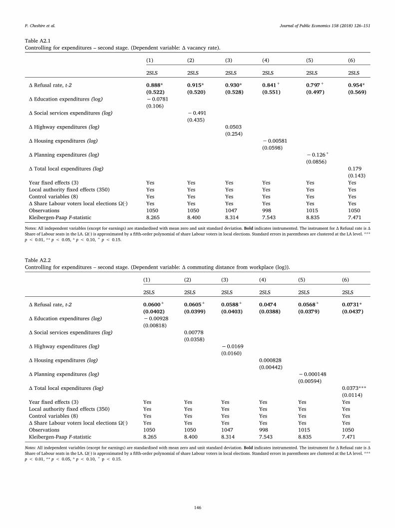
Table A2.1Controlling for expenditures – second stage. (Dependent variable: Δ vacancy rate).

(1) (2) (3) (4) (5) (6)

2SLS 2SLS 2SLS 2SLS 2SLS 2SLS

Δ Refusal rate, t-2 0.888* 0.915* 0.930* 0.841+ 0.797+ 0.954*(0.522) (0.520) (0.528) (0.551) (0.497) (0.569)

Δ Education expenditures (log) −0.0781(0.106)

Δ Social services expenditures (log) −0.491(0.435)

Δ Highway expenditures (log) 0.0503(0.254)

Δ Housing expenditures (log) −0.00581(0.0598)

Δ Planning expenditures (log) −0.126+

(0.0856)Δ Total local expenditures (log) 0.179

(0.143)Year fixed effects (3) Yes Yes Yes Yes Yes YesLocal authority fixed effects (350) Yes Yes Yes Yes Yes YesControl variables (8) Yes Yes Yes Yes Yes YesΔ Share Labour voters local elections Ω(∙) Yes Yes Yes Yes Yes YesObservations 1050 1050 1047 998 1015 1050Kleibergen-Paap F-statistic 8.265 8.400 8.314 7.543 8.835 7.471

Notes: All independent variables (except for earnings) are standardised with mean zero and unit standard deviation. Bold indicates instrumented. The instrument for Δ Refusal rate is ΔShare of Labour seats in the LA. Ω(∙) is approximated by a fifth-order polynomial of share Labour voters in local elections. Standard errors in parentheses are clustered at the LA level. ***p < 0.01, ** p < 0.05, * p < 0.10, + p < 0.15.

Table A2.2Controlling for expenditures – second stage. (Dependent variable: Δ commuting distance from workplace (log)).

(1) (2) (3) (4) (5) (6)

2SLS 2SLS 2SLS 2SLS 2SLS 2SLS

Δ Refusal rate, t-2 0.0600+ 0.0605+ 0.0588+ 0.0474 0.0568+ 0.0731*(0.0402) (0.0399) (0.0403) (0.0388) (0.0379) (0.0437)

Δ Education expenditures (log) −0.00928(0.00818)

Δ Social services expenditures (log) 0.00778(0.0358)

Δ Highway expenditures (log) −0.0169(0.0160)

Δ Housing expenditures (log) 0.000828(0.00442)

Δ Planning expenditures (log) −0.000148(0.00594)

Δ Total local expenditures (log) 0.0373***(0.0114)

Year fixed effects (3) Yes Yes Yes Yes Yes YesLocal authority fixed effects (350) Yes Yes Yes Yes Yes YesControl variables (8) Yes Yes Yes Yes Yes YesΔ Share Labour voters local elections Ω(∙) Yes Yes Yes Yes Yes YesObservations 1050 1050 1047 998 1015 1050Kleibergen-Paap F-statistic 8.265 8.400 8.314 7.543 8.835 7.471

Notes: All independent variables (except for earnings) are standardised with mean zero and unit standard deviation. Bold indicates instrumented. The instrument for Δ Refusal rate is ΔShare of Labour seats in the LA. Ω(∙) is approximated by a fifth-order polynomial of share Labour voters in local elections. Standard errors in parentheses are clustered at the LA level. ***p < 0.01, ** p < 0.05, * p < 0.10, + p < 0.15.

P. Cheshire et al. Journal of Public Economics 158 (2018) 126–151

146

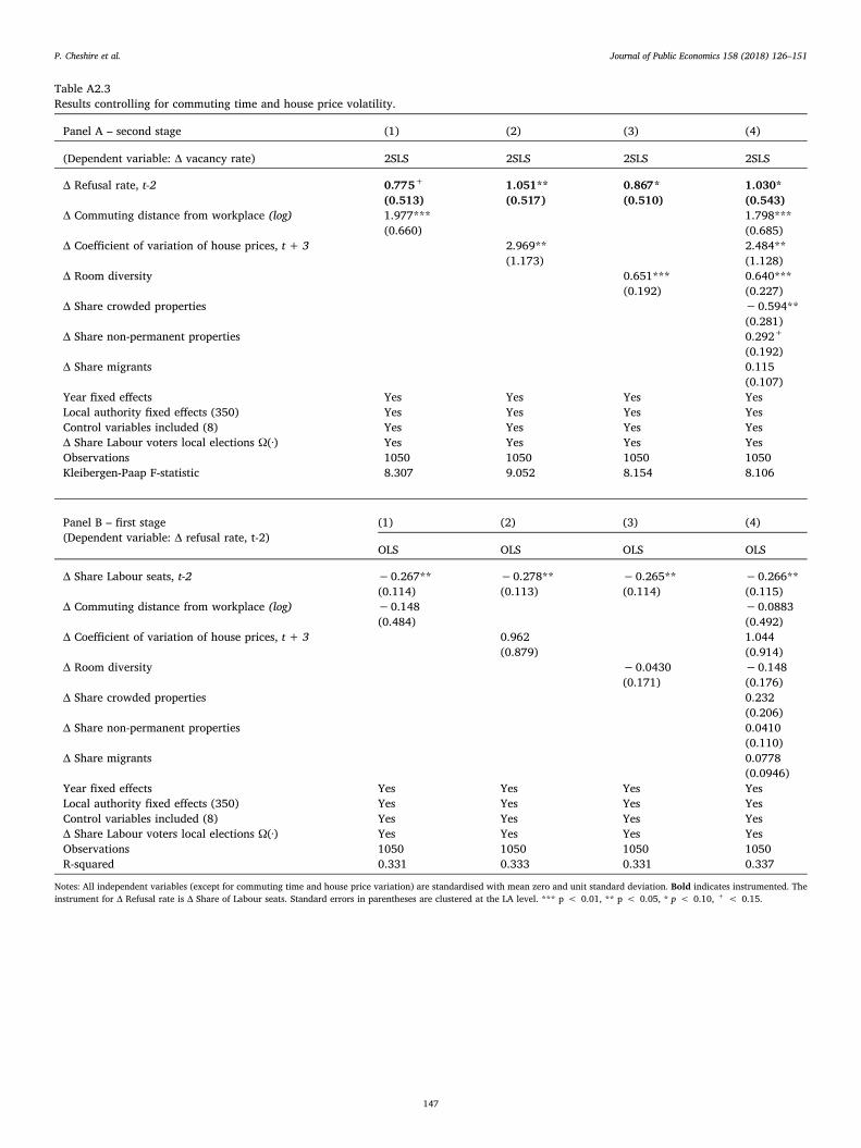
Table A2.3Results controlling for commuting time and house price volatility.

Panel A – second stage (1) (2) (3) (4)

(Dependent variable: Δ vacancy rate) 2SLS 2SLS 2SLS 2SLS

Δ Refusal rate, t-2 0.775+ 1.051** 0.867* 1.030*(0.513) (0.517) (0.510) (0.543)

Δ Commuting distance from workplace (log) 1.977*** 1.798***(0.660) (0.685)

Δ Coefficient of variation of house prices, t + 3 2.969** 2.484**(1.173) (1.128)

Δ Room diversity 0.651*** 0.640***(0.192) (0.227)

Δ Share crowded properties −0.594**(0.281)

Δ Share non-permanent properties 0.292+

(0.192)Δ Share migrants 0.115

(0.107)Year fixed effects Yes Yes Yes YesLocal authority fixed effects (350) Yes Yes Yes YesControl variables included (8) Yes Yes Yes YesΔ Share Labour voters local elections Ω(∙) Yes Yes Yes YesObservations 1050 1050 1050 1050Kleibergen-Paap F-statistic 8.307 9.052 8.154 8.106

Panel B – first stage(Dependent variable: Δ refusal rate, t-2)

(1) (2) (3) (4)

OLS OLS OLS OLS

Δ Share Labour seats, t-2 −0.267** −0.278** −0.265** −0.266**(0.114) (0.113) (0.114) (0.115)

Δ Commuting distance from workplace (log) −0.148 −0.0883(0.484) (0.492)

Δ Coefficient of variation of house prices, t + 3 0.962 1.044(0.879) (0.914)

Δ Room diversity −0.0430 −0.148(0.171) (0.176)

Δ Share crowded properties 0.232(0.206)

Δ Share non-permanent properties 0.0410(0.110)

Δ Share migrants 0.0778(0.0946)

Year fixed effects Yes Yes Yes YesLocal authority fixed effects (350) Yes Yes Yes YesControl variables included (8) Yes Yes Yes YesΔ Share Labour voters local elections Ω(∙) Yes Yes Yes YesObservations 1050 1050 1050 1050R-squared 0.331 0.333 0.331 0.337

Notes: All independent variables (except for commuting time and house price variation) are standardised with mean zero and unit standard deviation. Bold indicates instrumented. Theinstrument for Δ Refusal rate is Δ Share of Labour seats. Standard errors in parentheses are clustered at the LA level. *** p < 0.01, ** p < 0.05, * p < 0.10, + < 0.15.

P. Cheshire et al. Journal of Public Economics 158 (2018) 126–151

147

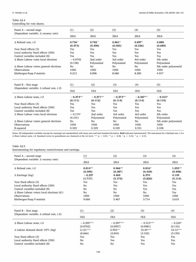
Table A2.4Controlling for vote shares.

Panel A – second stage(Dependent variable: Δ vacancy rate)

(1) (2) (3) (4) (5)

2SLS 2SLS 2SLS 2SLS 2SLS

Δ Refusal rate, t-2 0.756+ 0.782+ 0.861* 0.897* 0.888(0.473) (0.490) (0.505) (0.526) (0.689)

Year fixed effects (3) Yes Yes Yes Yes YesLocal authority fixed effects (350) Yes Yes Yes Yes YesControl variables included (8) Yes Yes Yes Yes YesΔ Share Labour votes local elections −0.0742 2nd order 3rd order 4rd order 5th order

(0.158) Polynomial Polynomial Polynomial PolynomialΔ Share Labour voters general elections No No No No 5th order polynomialObservations 1050 1050 1050 1050 1050Kleibergen-Paap F-statistic 9.213 8.896 8.680 8.285 4.917

Panel B – first stage(Dependent variable: Δ refusal rate, t-2)

(1) (2) (3) (4) (5)

OLS OLS OLS OLS OLS

Δ Share Labour seats, t-2 −0.274** −0.271** −0.273** −0.267** −0.215*(0.111) (0.112) (0.114) (0.114) (0.119)

Year fixed effects (3) Yes Yes Yes Yes YesLocal authority fixed effects (350) Yes Yes Yes Yes YesControl variables included (8) Yes Yes Yes Yes YesΔ Share Labour votes local elections −0.174* 2nd order 3rd order 4rd order 5th order

(0.101) Polynomial Polynomial Polynomial PolynomialΔ Share Labour voters general elections No No No No 5th order polynomialObservations 1050 1050 1050 1050 1050R-squared 0.329 0.329 0.329 0.331 0.338

Notes: All independent variables (except for earnings) are standardised with mean zero and unit standard deviation. Bold indicates instrumented. The instrument for Δ Refusal rate, t-2 isΔ Share Labour seats, t-2. Standard errors in parentheses are clustered at the LA level. *** p < 0.01, ** p < 0.05, * p < 0.10, + p < 0.15.

Table A2.5Instrumenting for regulatory restrictiveness and earnings.

Panel A – second stage(Dependent variable: Δ vacancy rate)

(1) (2) (3) (4)

2SLS 2SLS 2SLS 2SLS

Δ Refusal rate, t-2 0.814** 0.966** 0.816* 1.055**(0.390) (0.387) (0.439) (0.498)

Δ Earnings (log) −0.257 4.469 6.370 4.149(1.717) (5.170) (5.820) (5.114)

Year fixed effects (3) Yes Yes Yes YesLocal authority fixed effects (350) No Yes Yes YesControl variables included (8) No No Yes YesΔ Share Labour voters local elections Ω(∙) No No No YesObservations 1050 1050 1050 1050Kleibergen-Paap F-statistic 9.660 5.467 3.714 3.610

Panel B – first stage(Dependent variable: Δ refusal rate, t-2)

(1) (2) (3) (4)

OLS OLS OLS OLS

Δ Share Labour seats, t-2 −0.305*** −0.297*** −0.312*** −0.224*(0.0702) (0.0957) (0.0981) (0.116)

Δ Labour demand shock 1971 (log) 2.121*** 6.953** 10.29*** 10.12***(0.666) (2.843) (3.102) (3.159)

Year fixed effects (3) Yes Yes Yes YesLocal authority fixed effects (350) No Yes Yes YesControl variables included (8) No No Yes Yes

P. Cheshire et al. Journal of Public Economics 158 (2018) 126–151

148

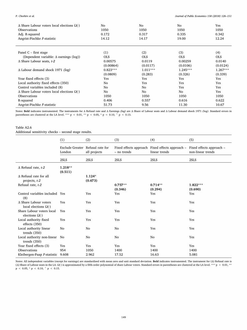
Δ Share Labour voters local elections Ω(∙) No No No YesObservations 1050 1050 1050 1050Adj. R-squared 0.172 0.317 0.335 0.342Angrist-Pischke F-statistic 14.12 14.17 19.00 12.24

Panel C – first stage(Dependent variable: Δ earnings (log))

(1) (2) (3) (4)OLS OLS OLS OLS

Δ Share Labour seats, t-2 0.00575 0.0119 0.00259 0.0140(0.00864) (0.0117) (0.0106) (0.0124)

Δ Labour demand shock 1971 (log) 0.823*** 1.011*** 1.245*** 1.267***(0.0809) (0.283) (0.326) (0.339)

Year fixed effects (3) Yes Yes Yes YesLocal authority fixed effects (350) No Yes Yes YesControl variables included (8) No No Yes YesΔ Share Labour voters local elections Ω(∙) No No No YesObservations 1050 1050 1050 1050R-squared 0.406 0.557 0.616 0.622Angrist-Pischke F-statistic 51.73 9.56 11.30 10.67

Notes: Bold indicates instrumented. The instruments for Δ Refusal rate and Δ Earnings (log) are Δ Share of Labour seats and Δ Labour demand shock 1971 (log). Standard errors inparentheses are clustered at the LA level. *** p < 0.01, ** p < 0.05, * p < 0.10, + p < 0.15.

Table A2.6Additional sensitivity checks – second stage results.

(1) (2) (3) (4) (5)

Exclude GreaterLondon

Refusal rate forall projects

Fixed effects approach– no trends

Fixed effects approach –linear trends

Fixed effects approach –non-linear trends

2SLS 2SLS 2SLS 2SLS 2SLS

Δ Refusal rate, t-2 1.218**(0.511)

Δ Refusal rate for allprojects, t-2

1.124*(0.673)

Refusal rate, t-2 0.757** 0.714** 1.822***(0.346) (0.294) (0.690)

Control variables included(8)

Yes Yes Yes Yes Yes

Δ Share Labour voterslocal elections Ω(∙)

Yes Yes Yes Yes Yes

Share Labour voters localelections Ω(∙)

Yes Yes Yes Yes Yes

Local authority fixedeffects (350)

Yes Yes Yes Yes Yes

Local authority lineartrends (350)

No No No Yes Yes

Local authority non-lineartrends (350)

No No No No Yes

Year fixed effects (3) Yes Yes Yes Yes YesObservations 954 1050 1400 1400 1400Kleibergen-Paap F-statistic 9.608 2.962 17.52 16.63 5.081

Notes: All independent variables (except for earnings) are standardised with mean zero and unit standard deviation. Bold indicates instrumented. The instrument for (Δ) Refusal rate is(Δ) Share of Labour seats in the LA. Ω(∙) is approximated by a fifth-order polynomial of share Labour voters. Standard errors in parentheses are clustered at the LA level. *** p < 0.01, **p < 0.05, * p < 0.10, + p < 0.15.

P. Cheshire et al. Journal of Public Economics 158 (2018) 126–151

149

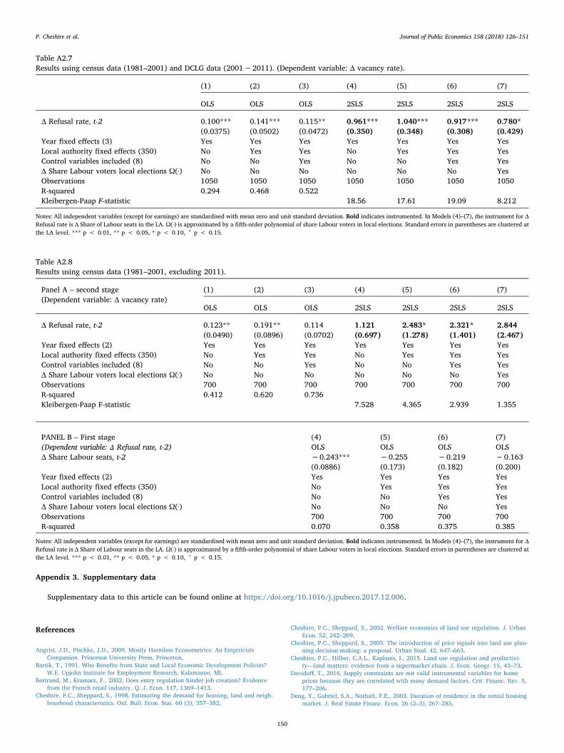
Table A2.7Results using census data (1981–2001) and DCLG data (2001−2011). (Dependent variable: Δ vacancy rate).

(1) (2) (3) (4) (5) (6) (7)

OLS OLS OLS 2SLS 2SLS 2SLS 2SLS

Δ Refusal rate, t-2 0.100*** 0.141*** 0.115** 0.961*** 1.040*** 0.917*** 0.780*(0.0375) (0.0502) (0.0472) (0.350) (0.348) (0.308) (0.429)

Year fixed effects (3) Yes Yes Yes Yes Yes Yes YesLocal authority fixed effects (350) No Yes Yes No Yes Yes YesControl variables included (8) No No Yes No No Yes YesΔ Share Labour voters local elections Ω(∙) No No No No No No YesObservations 1050 1050 1050 1050 1050 1050 1050R-squared 0.294 0.468 0.522Kleibergen-Paap F-statistic 18.56 17.61 19.09 8.212

Notes: All independent variables (except for earnings) are standardised with mean zero and unit standard deviation. Bold indicates instrumented. In Models (4)–(7), the instrument for ΔRefusal rate is Δ Share of Labour seats in the LA. Ω(∙) is approximated by a fifth-order polynomial of share Labour voters in local elections. Standard errors in parentheses are clustered atthe LA level. *** p < 0.01, ** p < 0.05, * p < 0.10, + p < 0.15.

Table A2.8Results using census data (1981–2001, excluding 2011).

Panel A – second stage(Dependent variable: Δ vacancy rate)

(1) (2) (3) (4) (5) (6) (7)

OLS OLS OLS 2SLS 2SLS 2SLS 2SLS

Δ Refusal rate, t-2 0.123** 0.191** 0.114 1.121 2.483* 2.321* 2.844(0.0490) (0.0896) (0.0702) (0.697) (1.278) (1.401) (2.467)

Year fixed effects (2) Yes Yes Yes Yes Yes Yes YesLocal authority fixed effects (350) No Yes Yes No Yes Yes YesControl variables included (8) No No Yes No No Yes YesΔ Share Labour voters local elections Ω(∙) No No No No No No YesObservations 700 700 700 700 700 700 700R-squared 0.412 0.620 0.736Kleibergen-Paap F-statistic 7.528 4.365 2.939 1.355

PANEL B – First stage (4) (5) (6) (7)(Dependent variable: Δ Refusal rate, t-2) OLS OLS OLS OLSΔ Share Labour seats, t-2 −0.243*** −0.255 −0.219 −0.163

(0.0886) (0.173) (0.182) (0.200)Year fixed effects (2) Yes Yes Yes YesLocal authority fixed effects (350) No Yes Yes YesControl variables included (8) No No Yes YesΔ Share Labour voters local elections Ω(∙) No No No YesObservations 700 700 700 700R-squared 0.070 0.358 0.375 0.385

Notes: All independent variables (except for earnings) are standardised with mean zero and unit standard deviation. Bold indicates instrumented. In Models (4)–(7), the instrument for ΔRefusal rate is Δ Share of Labour seats in the LA. Ω(∙) is approximated by a fifth-order polynomial of share Labour voters in local elections. Standard errors in parentheses are clustered atthe LA level. *** p < 0.01, ** p < 0.05, * p < 0.10, + p < 0.15.

Appendix 3. Supplementary data

Supplementary data to this article can be found online at https://doi.org/10.1016/j.jpubeco.2017.12.006.

References

Angrist, J.D., Pischke, J.D., 2009. Mostly Harmless Econometrics: An EmpiricistsCompanion. Princeton University Press, Princeton.

Bartik, T., 1991. Who Benefits from State and Local Economic Development Policies?W.E. Upjohn Institute for Employment Research, Kalamazoo, MI.

Bertrand, M., Kramarz, F., 2002. Does entry regulation hinder job creation? Evidencefrom the French retail industry. Q. J. Econ. 117, 1369–1413.

Cheshire, P.C., Sheppard, S., 1998. Estimating the demand for housing, land and neigh-bourhood characteristics. Oxf. Bull. Econ. Stat. 60 (3), 357–382.

Cheshire, P.C., Sheppard, S., 2002. Welfare economics of land use regulation. J. UrbanEcon. 52, 242–269.

Cheshire, P.C., Sheppard, S., 2005. The introduction of price signals into land use plan-ning decision-making: a proposal. Urban Stud. 42, 647–663.

Cheshire, P.C., Hilber, C.A.L., Kaplanis, I., 2015. Land use regulation and productivi-ty—land matters: evidence from a supermarket chain. J. Econ. Geogr. 15, 43–73.

Davidoff, T., 2016. Supply constraints are not valid instrumental variables for homeprices because they are correlated with many demand factors. Crit. Financ. Rev. 5,177–206.

Deng, Y., Gabriel, S.A., Nothaft, F.E., 2003. Duration of residence in the rental housingmarket. J. Real Estate Financ. Econ. 26 (2–3), 267–285.

P. Cheshire et al. Journal of Public Economics 158 (2018) 126–151

150

Department of Transport, 2013. Vehicle statistics. In: Statistics Information on Licensedand Unlicensed Vehicles, and MOT Testing, . https://www.gov.uk/government/collections/vehicles-statistics.

Ferreira, F., Gyourko, J., 2009. Do political parties matter? Evidence from U.S. cities. Q. J.Econ. 124 (1), 399–422.

Gabriel, S.A., Nothaft, F.E., 1988. Rental housing markets and the natural vacancy rate.Real Estate Econ. 16 (4), 419–429.

Gabriel, S.A., Nothaft, F.E., 2001. Rental housing markets, incidence and duration ofvacancy, and the natural vacancy rate. J. Urban Econ. 49, 121–149.

Glaeser, E.L., Gyourko, J., 2003. The impact of building restrictions on housing afford-ability. Econ. Policy Rev. 9, 21–39.

Glaeser, E.L., Gyourko, J., Saks, R.E., 2005a. Why have housing prices gone up? Am.Econ. Rev. 95 (2), 329–333.

Glaeser, E.L., Gyourko, J., Saks, R.E., 2005b. Why is Manhattan so expensive? Regulationand the rise in housing prices. J. Law Econ. 48, 331–369.

Glaeser, E.L., Gyourko, J., Saks, R.E., 2006. Urban growth and housing supply. J. Econ.Geogr. 6 (1), 71–89.

Government Office for the East Midlands, 2005. Regional Spatial Strategy for the EastMidlands (RSS8).

Grenadier, S.R., 1995. The persistence of real estate cycles. J. Real Estate Financ. Econ.10, 95–121.

Grenadier, S.R., 1996. The strategic exercise of options: development cascades andoverbuilding in real estate markets. J. Financ. 51 (5), 1653–1679.

Ha, S., Hilber, C.A.L., 2013. Do long distance moves discourage homeownership?Evidence from England. In: SERC Discussion Paper No. 141.

Han, L., Strange, W.C., 2015. The microstructure of housing markets: search, bargaining,and brokerage. In: Duranton, G., Henderson, J.V., Strange, W.C. (Eds.), Handbook ofRegional and Urban Economics. Vol. 5 Elsevier, Amsterdam.

Hilber, C.A.L., Robert-Nicoud, F., 2013. On the origins of land use regulations: theory andevidence from US metro areas. J. Urban Econ. 75 (1), 29–43.

Hilber, C.A.L., Vermeulen, W., 2016. The impact of supply constraints on house prices inEngland. Econ. J. 126 (591), 358–405.

Hilber, C.A.L., Lyytikäinen, T., Vermeulen, W., 2011. Capitalization of central govern-ment grants into local house prices: panel data evidence from England. Reg. Sci.Urban Econ. 41 (4), 394–406.

Ihlanfeldt, K.R., 2007. The effect of land use regulation on housing and land prices. J.

Urban Econ. 61, 420–435.Koster, H.R.A., Van Ommeren, J.N., 2017. On housing search frictions: Hedonic price

models, optimal search and welfare. In: Mimeo. Vrije Universiteit, Amsterdam.McDonald, R., Siegel, D., 1986. The value of waiting to invest. Q. J. Econ. 101, 707–727.Merlo, A., Ortalo-Magné, F., 2004. Bargaining over residential real estate: evidence from

England. J. Urban Econ. 56 (2), 192–216.Molloy, R., 2016. Long-term vacant housing in the United States. Reg. Sci. Urban Econ.

59, 118–129.Mortensen, D.T., Pissarides, C.A., 1994. Job creation and job destruction in the theory of

unemployment. Rev. Econ. Stud. 61 (3), 397–415.Mulalic, I., Van Ommeren, J.N., Pilegaard, N., 2014. Wages and commuting: quasi-natural

experiments' evidence from firms that relocate. Econ. J. 124, 1086–1105.ONS, 2016. The UK National Balance Sheet: 2016 estimates. Office of National Statistics,

London.Pawson, H., Kintrea, K., 2002. Part of the problem or part of the solution? Social housing

allocation policies and social exclusion in Britain. J. Soc. Policy 31 (4), 643–667.Pissarides, C.A., 1985. Short-run equilibrium dynamics of unemployment, vacancies, and

real wages. Am. Econ. Rev. 75 (4), 676–690.Pissarides, C.A., 1994. Search unemployment with on-the-job search. Rev. Econ. Stud. 61

(3), 457–475.Quigley, J.M., Raphael, S., 2005. Regulation and the high cost of housing in California.

Am. Econ. Rev. 95 (2), 323–328.Rallings, C., Thrasher, M. (Eds.), 2004. Local Elections in Britain: A Statistical Digest.

Local Government Chronicle Elections Centre, Plymouth.Rosen, K.T., Smith, L.B., 1983. The price-adjustment process for rental housing and the

natural vacancy rate. Am. Econ. Rev. 73 (4), 779–786.Sadun, R., 2015. Does planning regulation protect independent retailers? Rev. Econ. Stat.

97, 983–1001.Saks, R.E., 2008. Job creation and housing construction: constraints on metropolitan area

employment growth. J. Urban Econ. 64 (1), 178–195.Turner, M.A., Haughwout, A., Van Der Klaauw, W., 2014. Land use regulation and wel-

fare. Econometrica 82 (4), 1341–1403.Wall, D., 1998. The development of a land registry-based national house price index.

Econ. Trends 541 (12), 57–61.Wheaton, W.C., 1990. Vacancy, search, and prices in a housing market matching model.

J. Polit. Econ. 98 (6), 1270–1292.

P. Cheshire et al. Journal of Public Economics 158 (2018) 126–151

151