Department of Computer Science and Engineering

University of Moratuwa

CS4202 - Research and Development Project

Pattern Mining Based Automated Query Generation for

Complex Event Processing

Group Members

120418H Navagamuwa R. N

120468J Perera K. J. P. G

120555A Sally M. R. M. J

120488U Prashan L. A. V. N

Supervisors

Internal Dr. H.M.N. Dilum Bandara

External Dr. Srinath Perera, WSO2

Coordinated by

Dr. Charith Chitraranjan

THIS REPORT IS SUBMITTED IN PARTIAL FULFILMENT OF THE

REQUIREMENTS FOR THE AWARD OF THE DEGREE OF BACHELOR OF

SCIENCE OF ENGINEERING AT UNIVERSITY OF MORATUWA, SRI LANKA.

February 16, 2017

I

DECLARATION

We declare that this is our own work and this thesis does not incorporate without

acknowledgement any material previously submitted for a Degree or Diploma in any

other University or institute of higher learning and to the best of our knowledge and

belief it does not contain any material previously published or written by another

person except where the acknowledgement is made in the text. Also, we hereby grant

to University of Moratuwa the non-exclusive right to reproduce and distribute our

thesis, in whole or in part in print, electronic or other medium. We retain the right to

use this content in whole or part in future works (such as articles or books).

Signatures of the candidates:

.......................................................

R.N.Navagamuwa [120418H]

.......................................................

K.J.P.G. Perera [120468J]

.......................................................

M.R.M.J Sally [120555A]

.......................................................

L.A.V.N. Prashan [120488U]

Supervisor:

.......................................................

(Signature and Date)

Dr. H.M.N. Dilum Bandara

Coordinator:

.......................................................

(Signature and Date)

Dr. Charith Chitraranjan

II

ABSTRACT

Automating the query generation for Complex Event Processing (CEP) has marked its own

importance in allowing users to obtain useful insights from data. Existing techniques are both

computationally expensive and require extensive domain-specific human interaction. In

addressing these issues, we propose a technique that combines both parallel coordinates and

shapelets. First, if the provided data is not labeled (i.e., the time instances are not categorized

into specific events), we label the data by clustering the dataset into a set of clusters based

similarity between time instances. This produces a labeled dataset in which each time instance

is labeled with the respective event it belongs to. Next, each time instance of the labeled

multivariate dataset is represented as a line on a set of parallel coordinates. Then a shapelet-

learner algorithm is applied to those lines to extract the relevant shapelets. Afterwards, the

identified shapelets are ranked based on their information gain. Next, the shapelets with similar

information gain are grouped together by a shapelet-merger algorithm. The best group to

represent each event is then identified based on the event distribution of the dataset. Finally,

the best group is used to automatically generate the query to detect the complex events. The

proposed technique can be applied to both multivariate and multivariate time-series data, and

it is computationally and memory efficient. It enables users to focus only on the shapelets with

relevant information gains. We demonstrate the utility of the proposed technique using a set of

real-world datasets.

III

ACKNOWLEDGEMENT

First and foremost we would like to express our sincere gratitude to our project

supervisor, Dr. H.M.N. Dilum Bandara for the valuable guidance and dedicated

involvement at every step throughout the process.

We would also like to thank our external supervisor Dr. Srinath Perera for the valuable

advice and the direction given to us regarding the project.

In addition, we would like to thank Dr. Indika Perera and Dr. Surangika Ranathunga

for being panel members for our evaluations as well as for providing us with valuable

insights in the context of Complex Event Processing.

We would like to express our warm gratitude to Dr. Charith Chitraranjan for

coordinating the final year projects.

Last but not least, we would like to express our greatest gratitude to the Department of

Computer Science and Engineering, University of Moratuwa for providing the support

for us to successfully finish the project.

IV

TABLE OF CONTENT

DECLARATION ......................................................................................................... I

ABSTRACT ............................................................................................................... II

ACKNOWLEDGEMENT ....................................................................................... III

TABLE OF CONTENT ........................................................................................... IV

LIST OF FIGURES ................................................................................................. VI

LIST OF TABLES ................................................................................................. VII

LIST OF ABBREVIATIONS ............................................................................... VIII

1. INTRODUCTION .................................................................................................. 1

1.1 Background .................................................................................................... 1

1.2 Motivation ..................................................................................................... 1

1.3 Problem Statement ......................................................................................... 2

1.4 Objectives ...................................................................................................... 3

1.5 Research Contribution ................................................................................... 3

1.6 Outline ........................................................................................................... 4

2. LITERATURE REVIEW ...................................................................................... 5

2.1 Complex Event Processing ............................................................................ 5

2.2 Query Generation in CEP .............................................................................. 6

2.2.1 autoCEP Framework ............................................................................. 6

2.2.2 iCEP Framework ................................................................................... 9

2.2.3 CEP2U and CER Frameworks ............................................................ 12

2.2.4 User oriented rule management for event-based applications ............ 13

2.3 Query Optimization ..................................................................................... 14

2.3.1 Prediction correction paradigm ........................................................... 14

2.3.2 Iterative event pattern recommendation .............................................. 15

2.3.3 Distributed architecture for event-based systems................................ 15

2.3.4 Processing of uncertain events in a rule-based systems ...................... 16

2.4 Visualization tools ....................................................................................... 18

2.4.1 SPEEDD Framework .......................................................................... 18

2.4.2 Visualization Charts ............................................................................ 18

2.5 Pattern Mining Techniques .......................................................................... 19

V

2.5.1 Event sequence generation .................................................................. 19

2.5.2 Hidden Markov Model and Noise Hidden Markov Model ................. 19

2.5.3 Predictive complex event processing .................................................. 21

2.6 Unsupervised Clustering Techniques .......................................................... 21

2.6.1 DBSCAN Algorithm ........................................................................... 21

2.6.2 OPTICS Algorithm .............................................................................. 22

2.6.3 Single Linkage Clustering .................................................................... 24

3. METHODOLOGY ............................................................................................... 25

3.1 Preliminaries ................................................................................................ 25

3.1.1 Definitions ............................................................................................ 25

3.1.2 Shapelets............................................................................................... 26

3.1.3 Parallel Coordinates ............................................................................. 26

3.1.4 Problem Formulation............................................................................ 27

3.2 High-Level Design ...................................................................................... 28

3.3 Detailed Architecture .................................................................................. 36

3.3.1 Phase one: Shapelet Learner ................................................................ 37

3.3.2 Phase two Shapelet Extraction ............................................................. 39

3.3.3 Query Generation ................................................................................. 41

4. IMPLEMENTATION AND PERFORMANCE EVALUATION ................... 44

4.1 Web Application with spring ....................................................................... 44

4.2 Features of Web Application ....................................................................... 45

4.3 Screenshots of Web Application ................................................................. 46

4.3.1 Home Page ................................................................................................. 46

4.2.2 Shapelet Visualization ............................................................................... 47

4.4 Performance Evaluation .............................................................................. 48

5. SUMMARY........................................................................................................... 54

5.1 Conclusion ................................................................................................... 54

5.2 Future Work ................................................................................................. 55

References ................................................................................................................. 57

Appendix A: Accepted paper for IEEE International Conference on Smart Data

2016 ............................................................................................................................ 61

VI

LIST OF FIGURES

Figure 2.1: High-level architecture of autoCEP [2]. .................................................... 7

Figure 2.2: Illustration of best matching location [21]................................................. 8

Figure 2.3: iCEP architecture [2]. .............................................................................. 10

Figure 2.4: Executing the win learner [2]. ................................................................. 10

Figure 2.5: Evaluation architecture - iCEP [2]. .......................................................... 11

Figure 2.6: Rule-management workflows in existing systems (a) vs the proposed

approach (b) [7]. ......................................................................................................... 13

Figure 2.7: Prediction correction paradigm architecture [9]. ..................................... 14

Figure 2.8: Prefixspan algorithm [22]. ....................................................................... 19

Figure 2.9: Hidden Markov Model for pattern ABC [11]. ......................................... 20

Figure 2.10: Noise Hidden Markov Model [11]. ....................................................... 21

Figure 2.11: Hierarchically clustered city names using Single Linkage Clustering

[24]. ............................................................................................................................ 24

Figure 3.1: Time Series Shapelets.[5] ........................................................................ 26

Figure 3.2: Parallel coordinates - Occupancy Detection Dataset. .............................. 27

Figure 3.3: Proposed system architecture. ................................................................. 28

Figure 3.4: Distance matrix. ....................................................................................... 30

Figure 3.5: Multivariate time series mapped as parallel coordinates. ........................ 35

Figure 3.6: Shapelets slide across the time series. ..................................................... 35

Figure 3.7: Architecture - Shapelet generator module. .............................................. 37

Figure 4.1: Home page of Web application. .............................................................. 46

Figure 4.2: Event 0 (Occupied) - Shapelet representation. ........................................ 47

Figure 4.3: Event 1 (Non- Occupied) - Shapelet representation. ............................... 47

Figure 4.4: Extracted shapelets for Event 1 - Occupancy dataset. ............................. 50

Figure 4.5: Extracted shapelets for Event 2 - Occupancy dataset. ............................. 50

Figure 4.6: Extracted shapelets for Event 1 - EEG dataset. ....................................... 52

Figure 4.7 : Extracted shapelets for Event 2 - EEG dataset. ...................................... 52

VII

LIST OF TABLES

Table 4.1: Occupancy dataset clustering results. ....................................................... 48

Table 4.2: EEG dataset clustering results................................................................... 49

Table 4.3: Occupancy dataset event detection results. ............................................... 51

Table 4.4: EEG dataset event detection results. ......................................................... 53

VIII

LIST OF ABBREVIATIONS

API Application Programming Interface

ARFF Attribute Relation File Format

CEP Complex Event Processing

CORI Collection Retrieval Inference

CSV Comma Separated Values

CSS Cascading Style Sheets

DBSCAN Density Based Spatial Clustering of Applications with Noise

FHSAR For Hiding Service Association Rules

HMM Hidden Markov Model

HTML Hyper Text Markup Language

HTTP Hyper Text Transfer Protocol

IoT Internet of Things

JSON JavaScript Object Notation

JSP Java Server Pages

MVC Model View Controller

SPEEDD Scalable Proactive Event-Driven Decision-making

OPTICS Ordering points to identify the clustering structure

XSLT Extensible Stylesheet Language Transformations

XML Extensible Markup Language

1

Chapter 1

INTRODUCTION

1.1 Background

Automating query generation in large, multivariate datasets are useful in many

application domains. For example, Complex Event Processing (CEP) combines data

from multiple, streaming sources to identify meaningful events or patterns in real time.

While the detection of relevant events and patterns may give insight about

opportunities and threats related to the data being monitored (e.g., a set of sensor

readings and credit card transactions), significant domain knowledge is required to

write effective CEP queries. Manual analysis of data streams is not only tedious and

error prone, but also important events are likely to be missed due to the limited domain

knowledge of the query writer. A promising alternative is to automate the CEP query

generation by automatically extracting/mining interesting patterns from the past data

[1], [2], [3].

1.2 Motivation

Suppose there is multi-story building and multiple rooms in each floor. Each room has

smoke and temperature sensors. Suppose the owner wants to detect fire in the building.

A CEP engine can be used to detect fire and generate an alarm once the smoke sensor

is triggered and temperature is above a set threshold. However, it is nontrivial to decide

on a suitable temperature threshold, even if the building has experienced fire in the

past. Hence, significant domain knowledge/expertise is required to define such a query.

Even if defined, it may not be the most appropriate for the particular building.

Instead, it would be more useful to have a method which will generate these queries

automatically. One alternative is to look at the past data from all the sensors and

identify the typical behaviour. Anything that is different from this behaviour can be

flagged. In case if the data also have sensor readings during a past fire, those could be

flagged as outliers. Hence, it is possible to derive basic queries by looking at the data

alone. However, it is also important to separate out potential sensor errors/failures and

2

actual fires. If some domain expertise is available those queries could be further refined

based on user hints to improve detection rate and accuracy. This idea of automated

CEP query generation can be applied to many domains such as stock market, online

retail, and Internet of Things (IoT).

However, developing an automated query generation system that works across many

domains is not straightforward. Several related work has attempted to address this

problem with limited success. For example, AutoCEP [3] is one such approaches that

proposed a shapelet-based technique to automate CEP query generation for univariate

time series. This itself is a major limitation as the practical presence of univariate time

series is limited in CEP. Moreover, AutoCEP generates queries for each and every

instance of the detected event, requiring the CEP engine to concurrently process

multiple queries. This unnecessarily increases the computational and memory

requirements of the CEP engine and consequently degrades its performance. iCEP

framework [2] was developed to generate CEP queries automatically using a machine

learning model. One of the main drawbacks of iCEP framework is the need of multiple

historical datasets. As iCEP framework is based on a machine learning technique,

accuracy of the generated queries and event processing based on those queries

dependent on the comprehensiveness of the provided historical datasets. Ultra-fast

shapelets [4] is proposed for multivariate time-series classification, where it trains a

random forest to identify the shapelets with respect to the total dataset. While this

technique is effective in classification, it cannot be used to generate CEP queries, as

the generated random forest does not support backtracking and obtaining relevant

information to determine what data lead to the classification of the event.

1.3 Problem Statement

Given a sample dataset, we address the problem of auto generating relevant queries for

Complex Event Processors without having the exact domain knowledge. The specific

problem that this project aims to address can be stated as follows:

How to generate CEP queries for multivariate time series datasets that may or may

not be annotated without requiring expert domain knowledge?

3

In proposing the solution we assume that each instance in the obtained dataset is either

annotated according to the respective event or can be annotated with bit of effort. Our

goal is to construct a filter query per event, which contains the most relevant attributes,

their range of values, and the event detection time frame. Target is to develop a CEP

filter query similar to the following:

SELECT {∗} WHERE {attr1 ≥ a and attr2 < b} WITHIN {t1 ≤ time ≤ t2}

1.4 Objectives

Objectives of this research are to:

1. Develop a mechanism to convert datasets given in different formats to a

common format so that the later processing becomes simple

2. Use the data and pattern mining techniques to identify common patterns and

outliers in data

3. Implement a mechanism to obtain user hints and user given rules for generating

a query

4. Visualize the identified pattern results back to the user to obtain furthermore

insights and feedback

5. Automate the query generation for CEP

1.5 Research Contribution

We propose a technique that represents a given multivariate dataset as a set of parallel

coordinates, and then extract shapelets out of those coordinates to auto generate CEP

queries [5]. Even a time series can be mapped to a set of parallel coordinates, by

representing each time instance as a separate line. Extracted shapelets are sorted

according to the information gains and then divided into a set of groups. Among all

the groups, best group for each event is then identified. Then the most important

shapelets in the identified groups are used to generate one CEP query per group. This

enables one to generate CEP queries for commonalities, anomalies, as well as time-

series breakpoints in a given multivariate time-series dataset without having any

domain knowledge. Users can focus on groups with high or low information gain

4

depending on the application. Moreover, shapelets identify the most relevant attributes

in a dataset for a particular event, enabling us to write more efficient CEP queries and

only one query per event (unless the same event is triggered by unrelated attribute

combinations). Using a set of real-world datasets, we demonstrate that the proposed

technique can be applied effectively to auto generate CEP queries for common and

abnormal events while identifying the relevant features and event occurrence

timeframe. Moreover, the proposed technique has a relatively low computational and

memory requirements compared to prior work. Furthermore, to annotate datasets that

are not pre-annotated, we propose an unsupervised clustering technique that cluster a

numerical dataset without knowing the behaviour of a dataset or in other words,

without the interaction of a domain expert. The technique proposed by us initially

calculates the euclidean distances between time instances and the obtained distance

matrix will be clustered using OPTICS algorithm providing an annotation for each

time instance with respect to its belongingness to a particular event.

1.6 Outline

The remainder of the report is organized as follows. Chapter 2 provides a detailed

analysis of related work in CEP, query generation, query optimization, event detection,

visualization techniques, pattern mining techniques, and clustering techniques. High-

level design and detailed design of each module are presented in Chapter 3. Chapter 4

presents the implementation of the tool and performance analysis. Finally, we

summarize the work and discuss future work in Chapter 5.

5

Chapter 2

LITERATURE REVIEW

Section 2.1 describes Complex Event Processing and its usage in real world

applications. Next we discuss some related works which we have gone through.

Section 2.2 describes related work under query generation. Query optimization,

visualization tools, pattern mining techniques and unsupervised techniques are

presented in Section 2.3, Section 2.4, Section 2.5, and section 2.6 respectively.

2.1 Complex Event Processing

Complex Event Processing (CEP) refers to event processing that combines data from

multiple sources to detect events or patterns that suggest much more complicated

circumstances. Modern day CEP is used across many domains and applications with

the utmost objective of identifying meaningful events such as opportunities and threats

and in order to react to them as quickly as possible [6]. As an example CEP is

effectively and widely used in fraud detection where suppose a debit card has been

stolen and when it is entered to an automatic teller machine the pattern of entering pin

number, number of frequent withdrawals, etc., are analyzed and performed CEP to

detect fraudulent activities. This high importance that CEP possesses in today’s context

has demanded it to produce highly accurate results. To produce highly accurate results

simply the event processor should be accompanied with accurate query generation

mechanism.

Esper [16] and WSO2 CEP [14] are two of the leading CEP engines. Complex Event

Processor helps identify the most meaningful events and patterns from multiple data

sources, analyze their impacts, and act on them in real time. Most importantly, CEP

engine can be deployed in standalone or distributed modes. CEP engines can be

plugged into existing architectures, for e.g., WSO2 and Esper CEP engines can be

embeddable in existing Java-based architectures such as Java Application Servers or

Enterprise Service Bus.

6

2.2 Query Generation in CEP

In CEP systems, query processing takes place according to user-defined rules, which

specify the relationship between observed events and phenomena of interest. While

preparing queries to detect complex events, several questions such as the following

need to be answered:

● Which events are relevant to detect the phenomena of interest and which are

not?

● Which values should they carry?

● Do they need to appear in a specific, temporal order?

● How the query can be optimized so that the computing and memory

requirements are reduced?

Writing rules with such details may be challenging, even for domain experts.

Furthermore, the accuracy of the written queries will depend on the domain expertise

that the user possesses. If the query generation process can be automated, we could

enable wider use of CEP without domain expertise while simplifying the process and

increasing the accuracy.

Several related work try to automate the process to figure out answers to the above

mentioned questions. However, they rely on strict assumptions such as dataset is a

univariate time-series and end user will be a domain expert [3], [7], [8]. Furthermore,

most of the implementations have been domain dependent. Majority of the proposed

approaches focused on shortcomings of the manual rule specification, and have

concentrated on optimizing the query processing by focusing on a specific CEP engine,

which has its own rule definition language and query processing algorithms [1], [2].

Next, we discuss several selected related works on automated CEP query generation

and optimization.

2.2.1 autoCEP Framework

Mousheimish et al. [3] proposed autoCEP where initially it learns from histories, then

the rules are extracted, and finally deployed into CEP engines in an automatic manner

7

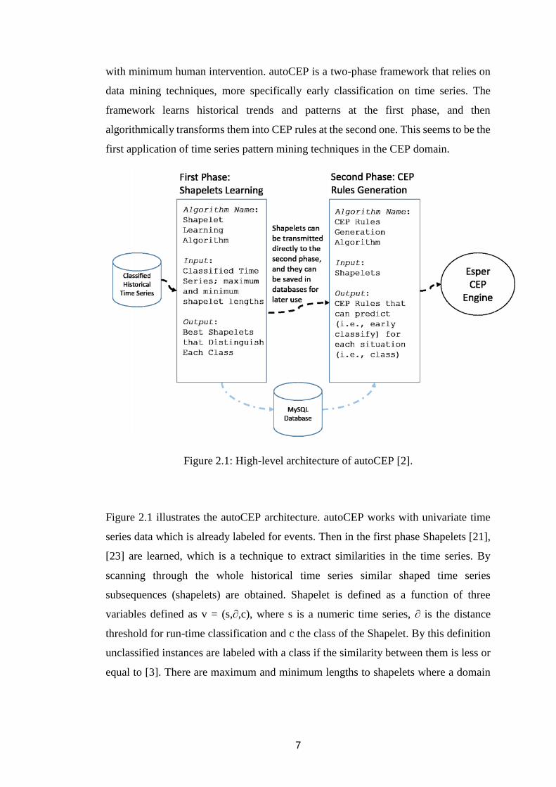
with minimum human intervention. autoCEP is a two-phase framework that relies on

data mining techniques, more specifically early classification on time series. The

framework learns historical trends and patterns at the first phase, and then

algorithmically transforms them into CEP rules at the second one. This seems to be the

first application of time series pattern mining techniques in the CEP domain.

Figure 2.1: High-level architecture of autoCEP [2].

Figure 2.1 illustrates the autoCEP architecture. autoCEP works with univariate time

series data which is already labeled for events. Then in the first phase Shapelets [21],

[23] are learned, which is a technique to extract similarities in the time series. By

scanning through the whole historical time series similar shaped time series

subsequences (shapelets) are obtained. Shapelet is defined as a function of three

variables defined as v = (s,∂,c), where s is a numeric time series, ∂ is the distance

threshold for run-time classification and c the class of the Shapelet. By this definition

unclassified instances are labeled with a class if the similarity between them is less or

equal to [3]. There are maximum and minimum lengths to shapelets where a domain

8

expert can specify them to have a better learning process. Then one can obtain the

useful shapelets that characterize each class and they are saved in a database (e.g.,

MySQL). Within the second phase of the implementation, rule generation using the

shapelets will take place which is done in a defined procedure. Prototype of the

generating rule is as follows:

within[window] {relevant events} where[conditions]

In this prototype within, {}, and where are the three main keywords for a generated rule

using a shapelet. Window and Conditions can be taken from the derived shapelets

saved in the MySQL database [3].

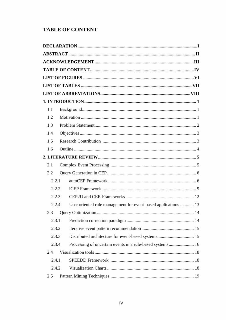
Figure 2.2: Illustration of best matching location [21].

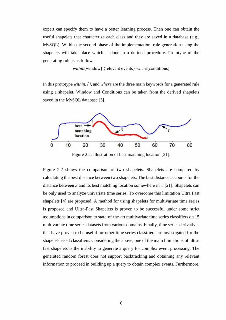
Figure 2.2 shows the comparison of two shapelets. Shapelets are compared by

calculating the best distance between two shapelets. The best distance accounts for the

distance between S and its best matching location somewhere in T [21]. Shapelets can

be only used to analyze univariate time series. To overcome this limitation Ultra Fast

shapelets [4] are proposed. A method for using shapelets for multivariate time series

is proposed and Ultra-Fast Shapelets is proven to be successful under some strict

assumptions in comparison to state-of-the-art multivariate time series classifiers on 15

multivariate time series datasets from various domains. Finally, time series derivatives

that have proven to be useful for other time series classifiers are investigated for the

shapelet-based classifiers. Considering the above, one of the main limitations of ultra-

fast shapelets is the inability to generate a query for complex event processing. The

generated random forest does not support backtracking and obtaining any relevant

information to proceed in building up a query to obtain complex events. Furthermore,

9

ultra-shapelet implementation also fails to identify data columns dynamically into the

shapelets.

2.2.2 iCEP Framework

iCEP [2] is a framework that has been developed using machine learning techniques

to determine the hidden causality between the events received from the external

environment and the situation to detect without the assistance of domain experts. iCEP

analyzes historical traces of events and effective use of supervised learning techniques

to derive relevant CEP rules. It is a highly modular system, with different components

considering different aspects of the rules. Depending on their knowledge of the

domain, users can decide which modules to deploy and can provide hints to guide the

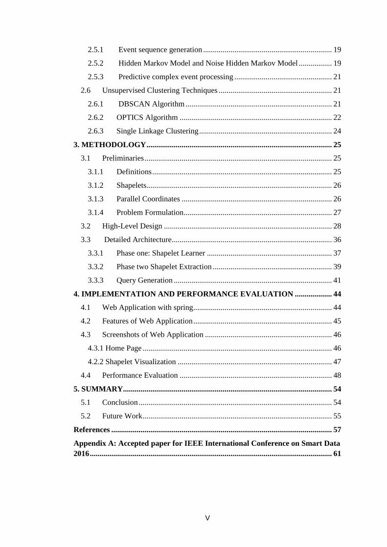
learning process and increase its precision [1], [2]. Figure 2.3 illustrates the high-level

architecture of iCEP which consists of seven different modules as follows:

1. Events and Attributes (Ev) Learner: finds which event types and attributes are

relevant for the rule.

2. Window (Win) Learner: finds the minimal time interval that includes all

relevant events.

3. Constraints (Constr) Learner: finds the constraints that select relevant events

based on the values of their attributes.

4. Aggregates (Agg) Learner: finds the presence and values of aggregate

constraints.

5. Parameters (Param) Learner: nds the parameters that bind the value of

attributes in different events.

6. Sequences (Seq) Learner: finds the ordering relations that hold among

primitive events.

7. Negations (Neg) Learner: finds negation constraints.

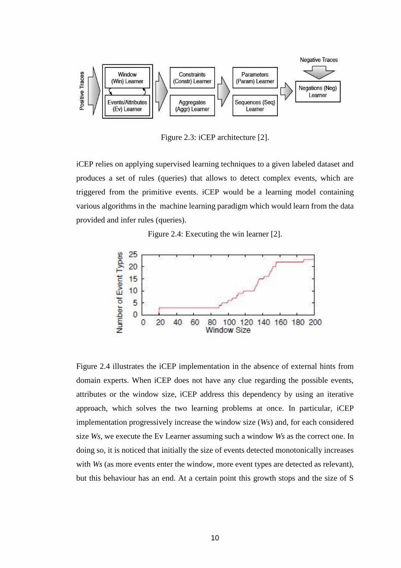
10

Figure 2.3: iCEP architecture [2].

iCEP relies on applying supervised learning techniques to a given labeled dataset and

produces a set of rules (queries) that allows to detect complex events, which are

triggered from the primitive events. iCEP would be a learning model containing

various algorithms in the machine learning paradigm which would learn from the data

provided and infer rules (queries).

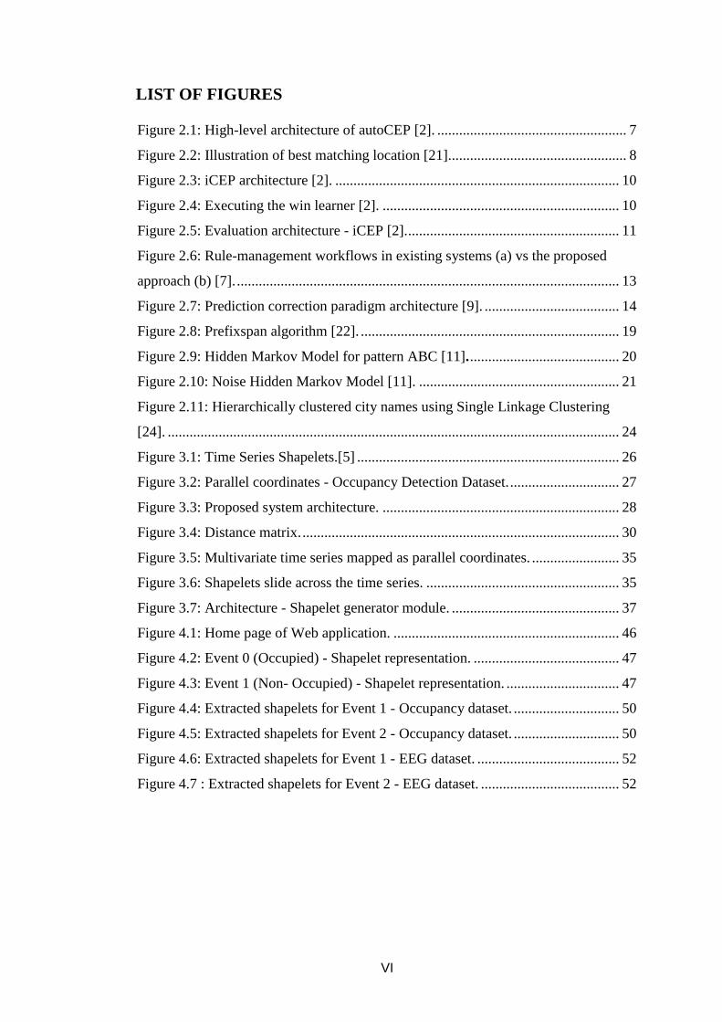
Figure 2.4: Executing the win learner [2].

Figure 2.4 illustrates the iCEP implementation in the absence of external hints from

domain experts. When iCEP does not have any clue regarding the possible events,

attributes or the window size, iCEP address this dependency by using an iterative

approach, which solves the two learning problems at once. In particular, iCEP

implementation progressively increase the window size (Ws) and, for each considered

size Ws, we execute the Ev Learner assuming such a window Ws as the correct one. In

doing so, it is noticed that initially the size of events detected monotonically increases

with Ws (as more events enter the window, more event types are detected as relevant),

but this behaviour has an end. At a certain point this growth stops and the size of S

11

stabilizes in a plateau. In practice, this happens when Ws reaches the value of the

window to learn.

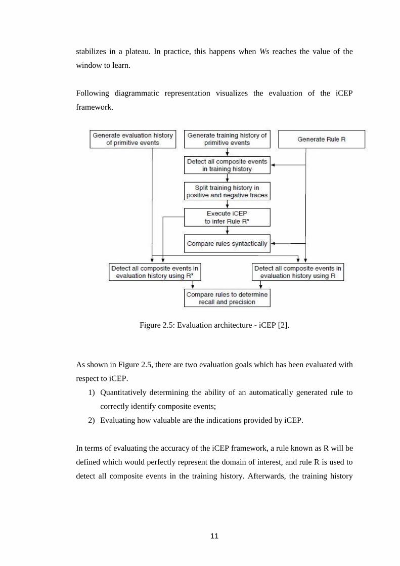
Following diagrammatic representation visualizes the evaluation of the iCEP

framework.

Figure 2.5: Evaluation architecture - iCEP [2].

As shown in Figure 2.5, there are two evaluation goals which has been evaluated with

respect to iCEP.

1) Quantitatively determining the ability of an automatically generated rule to

correctly identify composite events;

2) Evaluating how valuable are the indications provided by iCEP.

In terms of evaluating the accuracy of the iCEP framework, a rule known as R will be

defined which would perfectly represent the domain of interest, and rule R is used to

detect all composite events in the training history. Afterwards, the training history

12

(including primitive and composite events) is split to generate an (almost equal)

number of positive and negative traces of events. These traces will be the input to

iCEP, which uses them to infer a rule R∗. To quantitatively measure the performance

of iCEP following goal (a) above, we generate a new evaluation history of primitive

events, and using both R and R∗ to detect composite events over it. This allows us to

measure and recall our algorithm, which is the fraction of composite events captured

by R that have been also captured by R∗ and the precision, which is the fraction of

composite events captured by R∗ that actually occurred, i.e., that were also captured

by R. In terms of evaluating subjectively how capable iCEP at determining “correct”

rules along the lines of goal (b) above. To do so, we compare rules R and R∗

syntactically, to determine in which aspects they differ [1].

2.2.3 CEP2U and CER Frameworks

CEP2U [12] focuses on the following two possible sources of uncertainty:

● Uncertainty in events: The uncertainty deriving from an incorrect observation

of the phenomena under analysis. This means to admit that the notifications

entering the CEP engine can be characterized by a certain degree of

uncertainty.

● Uncertainty in rules: The uncertainty deriving from incomplete or erroneous

assumptions about the environment in which the system operates. This means

to admit that the CEP engine has only a partial knowledge about the system

under observation, and consequently the CEP rules cannot consider all the

factors that may cause the composite events they are in charge of detecting.

CEP2U models uncertainty in events using the theory of probability, while it exploits

Bayesian Networks (BNs) to model uncertainty in rules. In particular, it extends the

model of events to include probabilistic data into event notifications, while it

automatically builds a BN for each TESLA rule deployed in the system. Domain

experts are expected to extend such BNs to capture a priori knowledge about those

aspects of the environment that cannot be directly observed by sources.

13

Furthermore, in dealing with uncertainty regarding CEP, many of the CER engines

employ finite automata, either Deterministic (DFA) or Nondeterministic (NFA), as

well as logic based approaches are preferred [12].

2.2.4 User oriented rule management for event-based applications

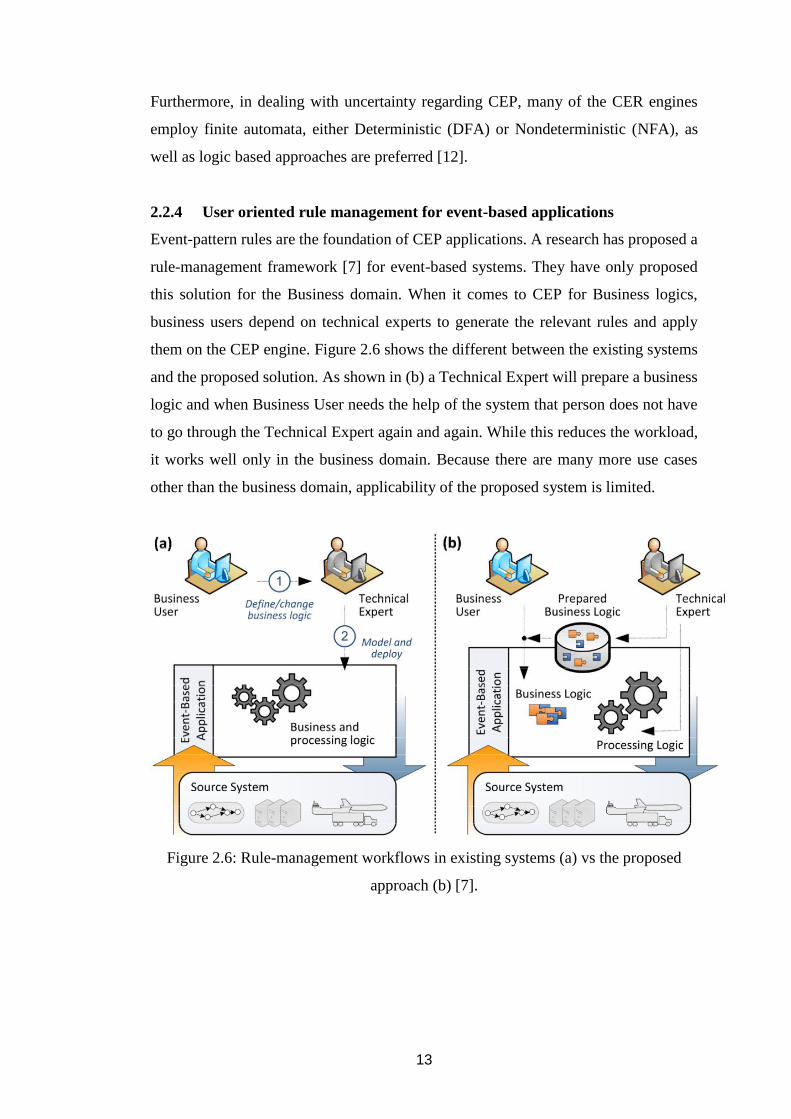
Event-pattern rules are the foundation of CEP applications. A research has proposed a

rule-management framework [7] for event-based systems. They have only proposed

this solution for the Business domain. When it comes to CEP for Business logics,

business users depend on technical experts to generate the relevant rules and apply

them on the CEP engine. Figure 2.6 shows the different between the existing systems

and the proposed solution. As shown in (b) a Technical Expert will prepare a business

logic and when Business User needs the help of the system that person does not have

to go through the Technical Expert again and again. While this reduces the workload,

it works well only in the business domain. Because there are many more use cases

other than the business domain, applicability of the proposed system is limited.

Figure 2.6: Rule-management workflows in existing systems (a) vs the proposed

approach (b) [7].

14

2.3 Query Optimization

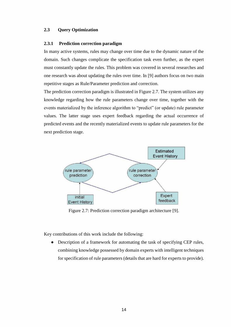
2.3.1 Prediction correction paradigm

In many active systems, rules may change over time due to the dynamic nature of the

domain. Such changes complicate the specification task even further, as the expert

must constantly update the rules. This problem was covered in several researches and

one research was about updating the rules over time. In [9] authors focus on two main

repetitive stages as Rule/Parameter prediction and correction.

The prediction correction paradigm is illustrated in Figure 2.7. The system utilizes any

knowledge regarding how the rule parameters change over time, together with the

events materialized by the inference algorithm to “predict” (or update) rule parameter

values. The latter stage uses expert feedback regarding the actual occurrence of

predicted events and the recently materialized events to update rule parameters for the

next prediction stage.

Figure 2.7: Prediction correction paradigm architecture [9].

Key contributions of this work include the following:

● Description of a framework for automating the task of specifying CEP rules,

combining knowledge possessed by domain experts with intelligent techniques

for specification of rule parameters (details that are hard for experts to provide).

15

● Description of a simple yet powerful model for rule parameter determination

and tuning, taking into account any pre-existing knowledge regarding the

updates of parameters over time, with indirect expert feedback.

● Provision of an algorithm based on Discrete Kalman Filters [13] to determine

and tune the parameter values.

2.3.2 Iterative event pattern recommendation

Not only CEP rules, CEP patterns may also change over time due to the dynamic nature

of the domain. So domain experts must update the patterns constantly. To overcome

this, some have come up with a solution which consists of Recommendation Based

Pattern Generation [10]. This research paper targets a specific domain which is

Ambient Assisted Living domain. This domain serves as an integration as well as the

evaluation platform. In order to speed up the pattern generation phase and help the

telecare solution and care providers, they believe that some kind of pattern

recommendation based on user input and existing patterns could be helpful. Authors

made the following contributions:

● An approach for supporting the domain expert in designing new patterns and

identifying missing ones

● Implementation of the approach for an use case example

● Evaluation results showing the importance of pattern recommendation during

the pattern generation process

2.3.3 Distributed architecture for event-based systems

When it comes to CEP, optimization is a major requirement and there has been so

many researches to optimize event-based systems. A research has been done targeting

distributed systems and some architectures to improve optimization [15] have been

suggested. According to them the following architectures can be used:

● Event-Driven Service Oriented Architecture

The event-driven SOA is an extension of the SOA re with event processing

capabilities. Services are entities that encapsulate business functionalities,

offered via described interfaces that are published, discovered and used by

16

clients. Events introduce a different interaction model in which event channels

allow consumers to subscribe for specific events, and receive them when such

events are published by producers. This mechanism is adopted in open

standards (e.g., CORBA), and in products or platforms (such as .NET,

WebSphere Business Events, Oracle CEP application server, and others) with

the aim of simplifying the design of complex interactions and supporting

interoperability.

● Grid Architecture

Event processing is useful in Data Grids, which allow users to access and

process large amounts of diverse data (files, databases, video streams, sensor

streams, and so forth) stored in distributed repositories. Data Grids include

services and infrastructure made available to user applications for executing

different operations such as data discovery, access, transfer, analysis,

visualization, transformation, and others.

● Peer-to-peer(P2P) Architecture

P2P systems are capable of adapting to failures and dynamic populations of

nodes while maintaining acceptable performance. P2P systems are used to

support application services for communication and collaboration, distributed

computation, content distribution, etc., and middleware services like routing

and location, anonymity, and privacy.

● Agent Architecture

Software agents react in response to other agents and to environment changes,

and can act independently (are autonomic). In addition, agents initiate actions

that affect the environment (are pro-active), are flexible (able to learn) and

cooperate with other agents in multi-agent systems.

2.3.4 Processing of uncertain events in a rule-based systems

There is a growing need for systems that react automatically to events. While some

events are generated externally and deliver data across distributed systems, others need

to be derived by the system itself based on available information. A research has

presented a mechanism to construct the probability space that captures the semantics

and defines the probabilities of possible worlds using an abstraction based on a

17

Bayesian network [19]. Solution is to generate the composite events by the system

itself. This solution faces the following two major challenges:

● Calculate event probabilities while taking into account various types of

uncertainty is not trivial.

● Timely response to events under a heavy load of incoming events from various

sources.

Authors have come up with a new sampling algorithm for efficient approximation of

new event derivation, enabling a quick computation of probabilities of set of rules,

rather than a Bayesian network. They have used the domain of Syndromic Surveillance

System (Bioterrorist attack) to validate their solution and have contributed to the CEP

domain by

● Describing a simple yet powerful generic model for representing the derivation

of new events under uncertainty

● Extending the notion of selectability, which exists also in the context of

deterministic event derivation to handle efficiently the derivation of uncertain

events. Selectability filters events that are irrelevant to derivation by some

rules.

● Proposing an algorithms for calculating selectability enable significant

computational improvements by ensuring that rules are not applied to events

which are irrelevant to new event derivation.

● Developing a Bayesian network representation to derive new events given the

arrival of an uncertain event and to compute its probability

● Developing a sampling algorithm for efficient approximation of new event

derivation enabling a quick computation of probabilities of a set of events by

sampling over the set of rules, rather than from a Bayesian network

● Demonstrating the scalability and accuracy of the sampling algorithm.

18

2.4 Visualization tools

2.4.1 SPEEDD Framework

Scalable Proactive Event-Driven Decision-making (SPEEDD) Framework [17]

focuses on proactive event driven computing which support autonomous or semi-

autonomous decision-making, including a body of tools. This is used to exploit the

forecast models and state predictions as a basis for decision-making. The visualization

component (dashboard) supports the human interpretation of decisions made in

runtime. It facilitates decision making process for business users by providing easily

comprehensible visualization of detected or forecasted situations along with output of

the automatic decision making component.

2.4.2 Visualization Charts

In order to implement visualization of our research application, we searched about

several APIs and libraries such as Google charts, ChartJS and Data-Driven Documents

(D3) library. ChartJS provides useful charts to draw graphs, but in our scenario we

need to find a chart which can be customize for the user on the web browser. In this

case, Google Charts API was not a good solution since it does not support in build

customizable charts.

D3 Library is a JavaScript Library which provides dynamic and interactive

visualizations in web browsers, and it is more customizable than Google charts [30].

In D3 graphs, user can select column values by drawing a rectangle. This helps to get

the range of column values, but it mostly rely on users input, which is not so good for

our scenario. If user select a wrong region of values, the accuracy of the final output

query will be changed. This can leads to many false positive or false negatives.

ChartJS is the most suitable API for our implementation because it is easy to

implement and customize. ChartJS also provide interactive visualization like above

mentioned libraries.

19

2.5 Pattern Mining Techniques

2.5.1 Event sequence generation

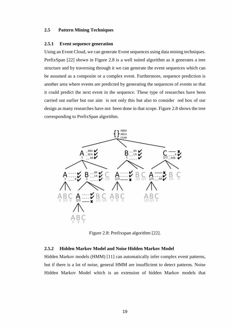
Using an Event Cloud, we can generate Event sequences using data mining techniques.

PrefixSpan [22] shown in Figure 2.8 is a well suited algorithm as it generates a tree

structure and by traversing through it we can generate the event sequences which can

be assumed as a composite or a complex event. Furthermore, sequence prediction is

another area where events are predicted by generating the sequences of events so that

it could predict the next event in the sequence. These type of researches have been

carried out earlier but our aim is not only this but also to consider red box of our

design as many researches have not been done in that scope. Figure 2.8 shows the tree

corresponding to PrefixSpan algorithm.

Figure 2.8: Prefixspan algorithm [22].

2.5.2 Hidden Markov Model and Noise Hidden Markov Model

Hidden Markov models (HMM) [11] can automatically infer complex event patterns,

but if there is a lot of noise, general HMM are insufficient to detect patterns. Noise

Hidden Markov Model which is an extension of hidden Markov models that

20

particularly addresses the problem of only sparsely occurring, significant events that

are interspersed with a lot of noise.

Hidden Markov Model (HMM) is a statistical model which is modeled using the

Markov model with visible (observed) states and hidden states. An HMM can be

represented as the simplest dynamic Bayesian network. It can addresses the following

three main problems [11]:

● Evaluation Problem - If we are given a sequence of visible states V, What is

the probability that the given V will be generated by given model H.

● Decoding Problem - What is the best state sequence for given model H.

● Learning Problem - How to calculate optimal model parameters for H that

maximize total production probability p(O|H)

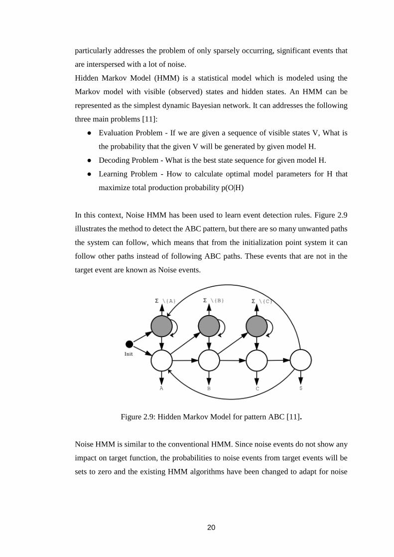
In this context, Noise HMM has been used to learn event detection rules. Figure 2.9

illustrates the method to detect the ABC pattern, but there are so many unwanted paths

the system can follow, which means that from the initialization point system it can

follow other paths instead of following ABC paths. These events that are not in the

target event are known as Noise events.

Figure 2.9: Hidden Markov Model for pattern ABC [11].

Noise HMM is similar to the conventional HMM. Since noise events do not show any

impact on target function, the probabilities to noise events from target events will be

sets to zero and the existing HMM algorithms have been changed to adapt for noise

21

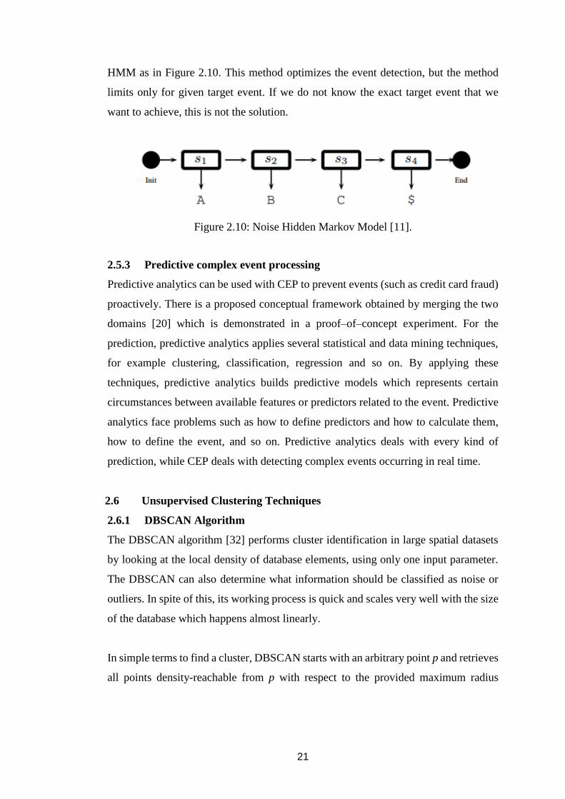
HMM as in Figure 2.10. This method optimizes the event detection, but the method

limits only for given target event. If we do not know the exact target event that we

want to achieve, this is not the solution.

Figure 2.10: Noise Hidden Markov Model [11].

2.5.3 Predictive complex event processing

Predictive analytics can be used with CEP to prevent events (such as credit card fraud)

proactively. There is a proposed conceptual framework obtained by merging the two

domains [20] which is demonstrated in a proof–of–concept experiment. For the

prediction, predictive analytics applies several statistical and data mining techniques,

for example clustering, classification, regression and so on. By applying these

techniques, predictive analytics builds predictive models which represents certain

circumstances between available features or predictors related to the event. Predictive

analytics face problems such as how to define predictors and how to calculate them,

how to define the event, and so on. Predictive analytics deals with every kind of

prediction, while CEP deals with detecting complex events occurring in real time.

2.6 Unsupervised Clustering Techniques

2.6.1 DBSCAN Algorithm

The DBSCAN algorithm [32] performs cluster identification in large spatial datasets

by looking at the local density of database elements, using only one input parameter.

The DBSCAN can also determine what information should be classified as noise or

outliers. In spite of this, its working process is quick and scales very well with the size

of the database which happens almost linearly.

In simple terms to find a cluster, DBSCAN starts with an arbitrary point p and retrieves

all points density-reachable from p with respect to the provided maximum radius

22

(Eps/𝜀) and minimum number of points (MinPts). If p is a core point, this procedure

yields a cluster with respect to 𝜀and MinPts. If p is a border point then no points are

density-reachable from p and DBSCAN visits the next point of the database.

2.6.2 OPTICS Algorithm

OPTICS algorithm [31] is an extended version of DBSCAN in which it works very

similar to DBSCAN algorithm for an infinite number of distance parameters

maximum radius (εi) which are smaller than a generating distance ε (i.e. 0 ≤ εi ≤ ε).

The only difference is that it does not assign cluster memberships. Instead, it stores the

order in which the objects are processed and the parameterized information would be

used by the algorithm to assign cluster memberships. Following defines and

explanations of basic definitions with respect to the OPTICS algorithm.

Definition 1: Directly density-reachable

Object p is directly density-reachable from object q wrt. ε and MinPts in a set of objects

D if

1. p ∈ Nε(q) (Nε(q) is the subset of D contained in the ε-neighborhood of q.)

2. Card(Nε(q)) ≥ MinPts (Card(N) denotes the cardinality of the set N)

The condition Card(Nε(q)) ≥ MinPts is called the core object condition. If this

condition holds for an object p, then we call p a core object. Only from core objects,

other objects can be directly density-reachable.

Definition 2: Density-reachable

An object p is density-reachable from an object q wrt. ε and MinPts in the set of objects

D if there is a chain of objects p1, ..., pn, p1 = q, pn = p such that pi ∈ D and pi+1 is

directly density-reachable from pi wrt. ε and MinPts.

Density-reachability is the transitive hull of direct density reachability. This relation is

not symmetric in general. Only core objects can be mutually density-reachable.

Definition 3: Density-connected

23

Object p is density-connected to object q wrt. ε and MinPts in the set of objects D if

there is an object o∈ D such that both p and q are density-reachable from o wrt. ε and

MinPts in D.

Definition 4: Cluster and noise

Let D be a set of objects. A cluster C wrt. ε and MinPts in D is a non-empty subset of

D satisfying the following conditions:

● Maximality: ∀p,q ∈D: if p ∈C and q is density-reachable from p wrt. ε and

MinPts, then also q ∈C.

● Connectivity: ∀p,q ∈ C: p is density-connected to q wrt. ε and MinPts in D.

Every object not contained in any cluster is noise.

Definition 5: Core-distance of an object p

Let p be an object from a database D, let ε be a distance value, let Nε(p) be the ε-

neighborhood of p, let MinPts be a natural number and let MinPts-distance(p) be the

distance from p to its MinPts’ neighbor. Then, the core-distance of p is defined as,

Core-distance𝜀,MinPts(p) =

{ 𝑴𝒊𝒏𝑷𝒕𝒔−𝑑𝑖𝑠𝑡𝑎𝑛𝑐𝑒 (𝑝) 𝑖𝑓 𝐶𝑎𝑟𝑑 (𝑁𝜀(𝑝)) ≥ 𝑀𝑖𝑛𝑃𝑡𝑠𝒖𝒏𝒅𝒆𝒇𝒊𝒏𝒆𝒅 𝑖𝑓 𝐶𝑎𝑟𝑑 (𝑁𝜀(𝑝)) < 𝑀𝑖𝑛𝑃𝑡𝑠

Definition 6: Reachability-distance object p w.r.t. object o

Let p and o be objects from a database D, let Nε(o) be the ε-neighborhood of o, and let

MinPts be a natural number. Then, the reachability-distance of p with respect to o is

defined as

reachability-distanceε,MinPts(p,o)=

{ 𝑚𝑎𝑥 𝑐𝑜𝑟𝑒−𝑑𝑖𝑠𝑡𝑎𝑛𝑐𝑒 (𝑜),𝑑𝑖𝑠𝑡𝑎𝑛𝑐𝑒 ( 𝑜,𝑝 ) ,𝑜𝑡ℎ𝑒𝑟𝑤𝑖𝑠𝑒𝑈𝑛𝑑𝑒𝑓𝑖𝑛𝑒𝑑 𝑖𝑓 | 𝑁𝜀 (𝑜)| < 𝑀𝑖𝑛𝑃𝑡𝑠

24

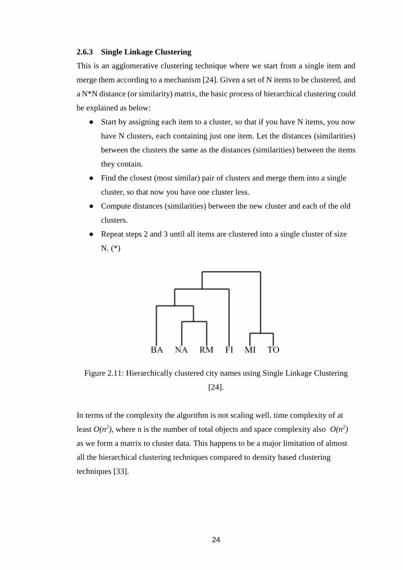
2.6.3 Single Linkage Clustering

This is an agglomerative clustering technique where we start from a single item and

merge them according to a mechanism [24]. Given a set of N items to be clustered, and

a N*N distance (or similarity) matrix, the basic process of hierarchical clustering could

be explained as below:

● Start by assigning each item to a cluster, so that if you have N items, you now

have N clusters, each containing just one item. Let the distances (similarities)

between the clusters the same as the distances (similarities) between the items

they contain.

● Find the closest (most similar) pair of clusters and merge them into a single

cluster, so that now you have one cluster less.

● Compute distances (similarities) between the new cluster and each of the old

clusters.

● Repeat steps 2 and 3 until all items are clustered into a single cluster of size

N. (*)

Figure 2.11: Hierarchically clustered city names using Single Linkage Clustering

[24].

In terms of the complexity the algorithm is not scaling well. time complexity of at

least O(n2), where n is the number of total objects and space complexity also O(n2)

as we form a matrix to cluster data. This happens to be a major limitation of almost

all the hierarchical clustering techniques compared to density based clustering

techniques [33].

25

Chapter 3

METHODOLOGY

In terms of auto generating relevant queries for CEP, we propose a technique based on

shapelets, parallel coordinates, and information gain. Section 3.1 introduces shapelets,

parallel coordinates, and problem formulation. High-level design of the proposed

solution is presented in Section 3.2. Detailed design is presented in Section 3.3.

3.1 Preliminaries

We first define relevant terms and then define shapelets and parallel coordinates as

applicable to the domain of CEP query generation. The research problem is then

formulated.

3.1.1 Definitions

Time-Series - A time-series T = t1, ..., tm is an ordered set of m real-valued variables.

Multivariate Time-Series — A multivariate time-series T = t1, ..., tm is a sequence of

m vectors, where ti = (ti,1, ..., ti,s) ∈ ℜ𝑠

with s attributes/variables.

Sub-sequence (𝑆𝑝𝑡) — Given a time-series T, a subsequence 𝑆𝑝

𝑡 of T is a sampling of

length l ≤ m of contiguous positions from T starting at time p, i.e., 𝑆𝑝𝑡 = tp, tp+1..., tp+l−1,

for 1 ≤ p ≤ m− l + 1.

Set of All Sub-sequences (STl) — Set of all possible subsequences 𝑆𝑝𝑡 that can be

extracted by sliding a window of length l across T is STl = {all 𝑆𝑝𝑡 of T, for 1 ≤ p ≤

m−l+1}.

Sub-sequence Distance — Given T and 𝑆𝑝𝑡 SubsequenceDist(T,𝑆𝑝

𝑡) is the minimum

distance between p contiguous positions obtained by sliding 𝑆𝑝𝑡 across T. We use

Euclidean distance as the distance function.

Entropy — Consider a time series dataset D consisting of two classes, A and B. Let

proportions of objects belonging to class A and B be p(A) and p(B), respectively. Then

the entropy of D is:

I(D) = −p(A)log(p(A)) − p(B)log(p(B)) (1)

26

Information Gain (Gain) — Given a certain split strategy sp which divides D into

two subsets D1 and D2, let the entropy before and after splitting be I(D) and 𝐼(D),

respectively. Then the information gain for split sp is:

Gain(sp) = I(D) − 𝐼(D)

Gain(sp) = I(D) − ( p(D1) I(D1) + p(D2) I(D2) ) (2)

Optimal Split Point (OSP) — Consider a time-series dataset D with two classes A

and B. For a given 𝑆𝑝𝑡 , we choose some distance threshold dth and split D into D1 and

D2, s.t. for every time series object T1,i in D1, SubsequenceDist(T1,i, 𝑆𝑝𝑡) ≤ dth and for

every T2,i in D2, SubsequenceDist(T2,i, 𝑆𝑝𝑡) ≥ dth. An Optimal Split Point (OSP) is a

distance threshold that Gain(𝑆𝑝𝑡 , dOSP (D,St p)) ≥ Gain(𝑆𝑝

𝑡 ,dth) for any other distance

threshold d-th.

3.1.2 Shapelets

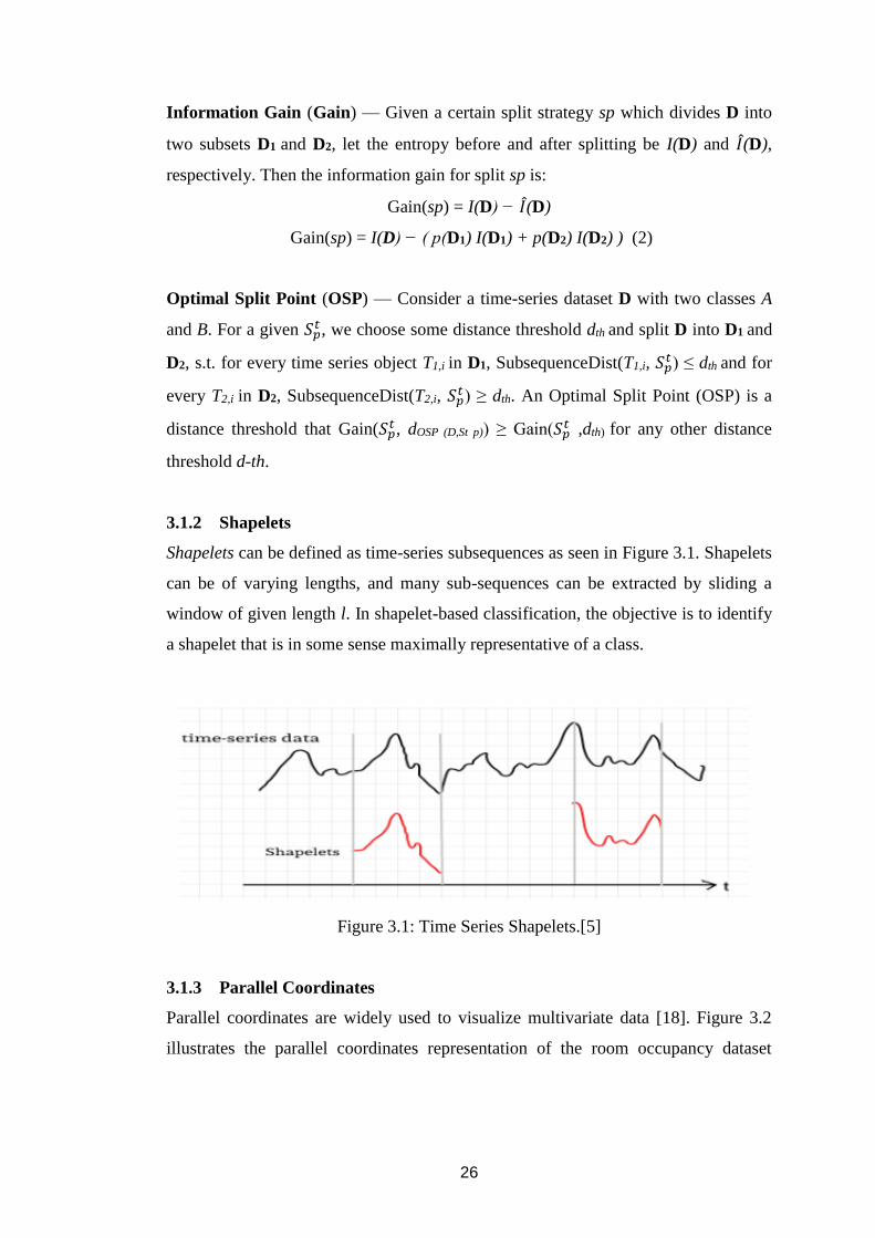
Shapelets can be defined as time-series subsequences as seen in Figure 3.1. Shapelets

can be of varying lengths, and many sub-sequences can be extracted by sliding a

window of given length l. In shapelet-based classification, the objective is to identify

a shapelet that is in some sense maximally representative of a class.

Figure 3.1: Time Series Shapelets.[5]

3.1.3 Parallel Coordinates

Parallel coordinates are widely used to visualize multivariate data [18]. Figure 3.2

illustrates the parallel coordinates representation of the room occupancy dataset

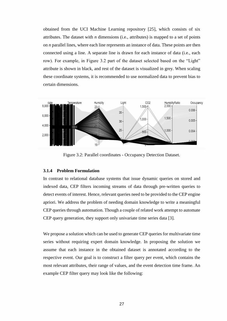
27

obtained from the UCI Machine Learning repository [25], which consists of six

attributes. The dataset with n dimensions (i.e., attributes) is mapped to a set of points

on n parallel lines, where each line represents an instance of data. These points are then

connected using a line. A separate line is drawn for each instance of data (i.e., each

row). For example, in Figure 3.2 part of the dataset selected based on the “Light”

attribute is shown in black, and rest of the dataset is visualized in grey. When scaling

these coordinate systems, it is recommended to use normalized data to prevent bias to

certain dimensions.

Figure 3.2: Parallel coordinates - Occupancy Detection Dataset.

3.1.4 Problem Formulation

In contrast to relational database systems that issue dynamic queries on stored and

indexed data, CEP filters incoming streams of data through pre-written queries to

detect events of interest. Hence, relevant queries need to be provided to the CEP engine

apriori. We address the problem of needing domain knowledge to write a meaningful

CEP queries through automation. Though a couple of related work attempt to automate

CEP query generation, they support only univariate time series data [3].

We propose a solution which can be used to generate CEP queries for multivariate time

series without requiring expert domain knowledge. In proposing the solution we

assume that each instance in the obtained dataset is annotated according to the

respective event. Our goal is to construct a filter query per event, which contains the

most relevant attributes, their range of values, and the event detection time frame. An

example CEP filter query may look like the following:

28

SELECT {∗} WHERE {attr1 ≥ a and attr2 < b} WITHIN {t1 ≤ time ≤ t2}

3.2 High-Level Design

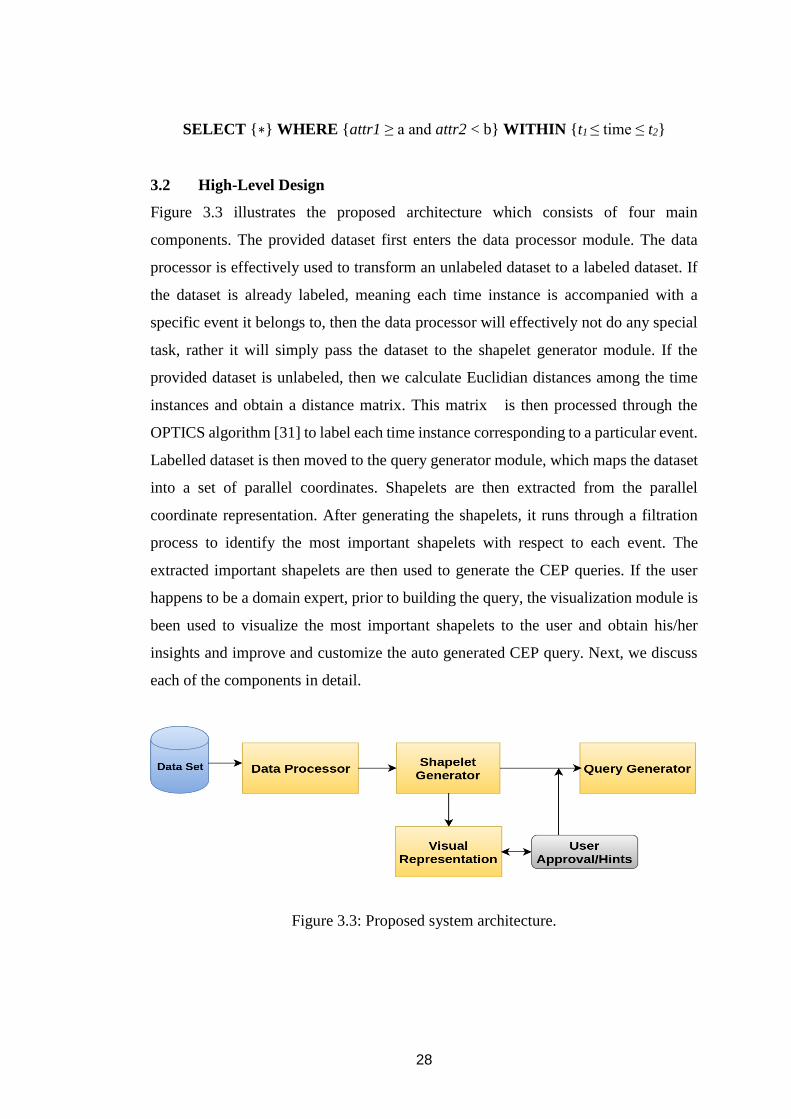
Figure 3.3 illustrates the proposed architecture which consists of four main

components. The provided dataset first enters the data processor module. The data

processor is effectively used to transform an unlabeled dataset to a labeled dataset. If

the dataset is already labeled, meaning each time instance is accompanied with a

specific event it belongs to, then the data processor will effectively not do any special

task, rather it will simply pass the dataset to the shapelet generator module. If the

provided dataset is unlabeled, then we calculate Euclidian distances among the time

instances and obtain a distance matrix. This matrix is then processed through the

OPTICS algorithm [31] to label each time instance corresponding to a particular event.

Labelled dataset is then moved to the query generator module, which maps the dataset

into a set of parallel coordinates. Shapelets are then extracted from the parallel

coordinate representation. After generating the shapelets, it runs through a filtration

process to identify the most important shapelets with respect to each event. The

extracted important shapelets are then used to generate the CEP queries. If the user

happens to be a domain expert, prior to building the query, the visualization module is

been used to visualize the most important shapelets to the user and obtain his/her

insights and improve and customize the auto generated CEP query. Next, we discuss

each of the components in detail.

Figure 3.3: Proposed system architecture.

29

3.2.1 Data Processor

First, the system identifies the dataset and convert that dataset into a generic format

before any further proceedings. The input dataset could be provided in any format (e.g.,

.txt, .xml, and .csv). Data Processor module converts the data to a generic format before

any further processing. This enables us to provide a solution that is applicable for

datasets from multiple domains, as well as supports both time-series datasets and none

time-series datasets.

We assume that each instance in the given dataset corresponds to an occurrence of a

specific event, i.e., each data instance is classified/labeled with the corresponding

event. The module then counts the number of events of each type, and their proportions

with respect to the total number of events in the entire dataset.

If the given dataset is not pre-annotated we propose a clustering-based technique to

annotate the dataset. Annotating each data point with the corresponding event is

important to calculate the information gain with respect to each shapelet, which is

required to filter out the generated shapelets to identify the most important shapelets.

The data processor then clusters the dataset, if the dataset provided is not already

labelled. Algorithm 3.1 initially calculates Euclidian distances between each pair of

time instances. The resulting distance matrix is then clustered using OPTICS algorithm

[31] resulting an annotation for each time instance. In doing so, the dataset in common

data format needs to be clustered in a manner in which each time instance is classified

with respect to an identified event. The output of the clustering technique would

modify the dataset by appending another column with numerical values to denote the

cluster number which indicate the event type that each column belongs to. This

information then will be effectively used in the information gain calculation step inside

the query generator module.

30

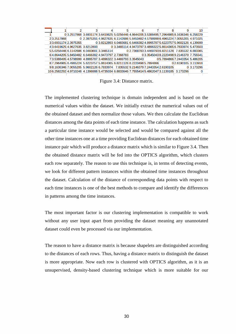
Figure 3.4: Distance matrix.

The implemented clustering technique is domain independent and is based on the

numerical values within the dataset. We initially extract the numerical values out of

the obtained dataset and then normalize those values. We then calculate the Euclidean

distances among the data points of each time instance. The calculation happens as such

a particular time instance would be selected and would be compared against all the

other time instances one at a time providing Euclidean distances for each obtained time

instance pair which will produce a distance matrix which is similar to Figure 3.4. Then

the obtained distance matrix will be fed into the OPTICS algorithm, which clusters

each row separately. The reason to use this technique is, in terms of detecting events,

we look for different pattern instances within the obtained time instances throughout

the dataset. Calculation of the distance of corresponding data points with respect to

each time instances is one of the best methods to compare and identify the differences

in patterns among the time instances.

The most important factor is our clustering implementation is compatible to work

without any user input apart from providing the dataset meaning any unannotated

dataset could even be processed via our implementation.

The reason to have a distance matrix is because shapelets are distinguished according

to the distances of each rows. Thus, having a distance matrix to distinguish the dataset

is more appropriate. Now each row is clustered with OPTICS algorithm, as it is an

unsupervised, density-based clustering technique which is more suitable for our

31

approach as shapelets are extracted according to their similarity of distances and

densities.

Then in the next iteration the base time instance will become the next time instance in

the dataset and the above process will continue as explained. At the end of each

iteration the obtained Euclidean distances per each time instance with respect to

selected base time instance, will be clustered using the OPTICS algorithm. The output

of the OPTICS algorithms clustering process would provide each time instance the

cluster that it belongs to which would update in a results array in which increments a

counter with respect to the relevant cluster and this will repeatedly happen with the

base time instance changing iteratively. After scanning through the entire dataset we

obtain the results array and scan through it and assign each time instance to the cluster

which has the highest count in terms of it belongingness. This value will be appended

to the dataset in which each time instance would have its corresponding event type.

Line 2 of the pseudo code representation of the clustering algorithm (Algorithm 3.1)

normalize the data and assign it to normData array. Then the for loop starting from

line 5 starts to scan through each element in normData and for each of the element of

this array we calculate Euclidean distance with all the other elements. The number of

times line 8 is executed equals to the array size. This allows us to obtain a distance

matrix. Afterwards, each of the rows in this distance matrix is processed through the

OPTICS algorithm to cluster which contains one-dimensional clustering of the

obtained distances. This is implemented in line 11 and 12. At the end, algorithm

analyses the row-wise cluster distribution and assigns each row for the respective

cluster which it happens to fall to most. The rest of the code is implemented such that

result array (line 4) is updated by giving the annotation.

In terms of clustering the obtained Euclidean distances, we went through the

implementations of popular unsupervised density based clustering techniques namely

DBSCAN [32], OPTICS, and Single-Linkage Clustering [33] which is a hierarchical

clustering technique. One of the main drawbacks in DBSCAN is we have to decide

parameters globally. Deciding parameters globally is utmost important in which

32

without it the hierarchical nature of densities could not be measured and in order to do

decide parameters globally we need to have an idea of the data distribution within the

dataset. Since from the beginning we intended to make the total implementation

domain and user independent obtaining information on the data distribution within the

dataset becomes infeasible and makes it even harder using DBSCAN. The reason

because DBSCAN cannot always be used to cluster data with different densities. So if

need to cluster data we need to know the densities of data so that we can give a suitable

𝜀 as a parameter.

For instance, within the DBSCAN implementation if a selected radius ‘r1’ is gives a

cluster named C and another radius ‘r2’ which is greater than ‘r1’ gives a separate

cluster named B, this would make C as a subset of B which limits the precision of the

derived clusters. This happens with inappropriate global parameter setting. This issue

of global parameter setting is overcome with OPTICS algorithm by iteratively

developing clusters starting from a small neighbourhood radius.

Furthermore, hierarchical clustering techniques also do provide satisfactory results but

with the limitation of high time and memory complexity compared to density based

methods. So to go line with our objective of finding time instances of similar patterns

which are dense around another time instance, hence it is required to cluster the

obtained Euclidean distance values considering the density and in doing so we did use

OPTICS algorithm which happens to be an extension of DBSCAN with overcoming

DBSCAN algorithm’s limitations.

In terms of user interaction with our system, in which the user happens to be a domain

expert that user could provide us with the additional information such as the number

of events within the dataset and proportionate event distribution to increase the

accuracy levels of the implementation. Conducting parameter tuning in the OPTICS

algorithm also allows a user to increase the accuracy levels of the clustering

implementation.

33

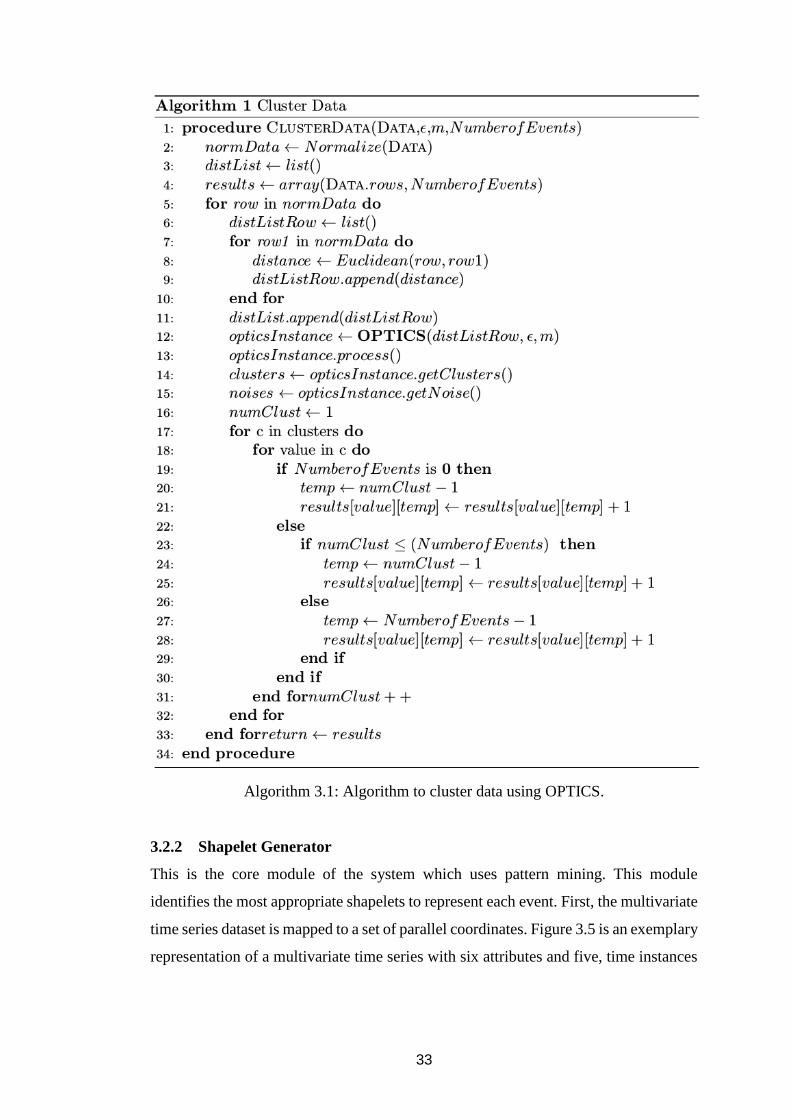
Algorithm 3.1: Algorithm to cluster data using OPTICS.

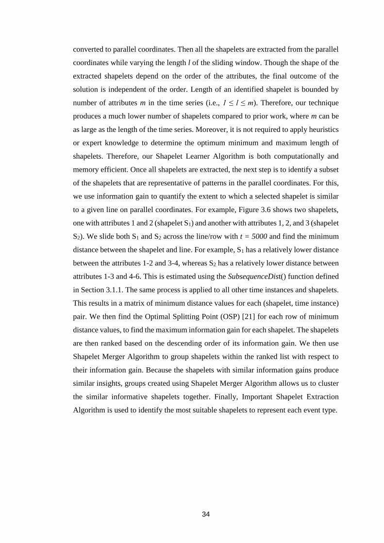
3.2.2 Shapelet Generator

This is the core module of the system which uses pattern mining. This module

identifies the most appropriate shapelets to represent each event. First, the multivariate

time series dataset is mapped to a set of parallel coordinates. Figure 3.5 is an exemplary

representation of a multivariate time series with six attributes and five, time instances

34

converted to parallel coordinates. Then all the shapelets are extracted from the parallel

coordinates while varying the length l of the sliding window. Though the shape of the

extracted shapelets depend on the order of the attributes, the final outcome of the

solution is independent of the order. Length of an identified shapelet is bounded by

number of attributes m in the time series (i.e., 1 ≤ l ≤ m). Therefore, our technique

produces a much lower number of shapelets compared to prior work, where m can be

as large as the length of the time series. Moreover, it is not required to apply heuristics

or expert knowledge to determine the optimum minimum and maximum length of

shapelets. Therefore, our Shapelet Learner Algorithm is both computationally and

memory efficient. Once all shapelets are extracted, the next step is to identify a subset

of the shapelets that are representative of patterns in the parallel coordinates. For this,

we use information gain to quantify the extent to which a selected shapelet is similar

to a given line on parallel coordinates. For example, Figure 3.6 shows two shapelets,

one with attributes 1 and 2 (shapelet S1) and another with attributes 1, 2, and 3 (shapelet

S2). We slide both S1 and S2 across the line/row with t = 5000 and find the minimum

distance between the shapelet and line. For example, S1 has a relatively lower distance

between the attributes 1-2 and 3-4, whereas S2 has a relatively lower distance between

attributes 1-3 and 4-6. This is estimated using the SubsequenceDist() function defined

in Section 3.1.1. The same process is applied to all other time instances and shapelets.

This results in a matrix of minimum distance values for each (shapelet, time instance)

pair. We then find the Optimal Splitting Point (OSP) [21] for each row of minimum

distance values, to find the maximum information gain for each shapelet. The shapelets

are then ranked based on the descending order of its information gain. We then use

Shapelet Merger Algorithm to group shapelets within the ranked list with respect to

their information gain. Because the shapelets with similar information gains produce

similar insights, groups created using Shapelet Merger Algorithm allows us to cluster

the similar informative shapelets together. Finally, Important Shapelet Extraction

Algorithm is used to identify the most suitable shapelets to represent each event type.

35

Figure 3.5: Multivariate time series mapped as parallel coordinates.

Figure 3.6: Shapelets slide across the time series.

3.2.3 Visual Representation

This module visualizes generated shapelets, optionally enabling users to select what

shapelets to choose for query writing. While the system can auto generate queries

without any user suggestions, this module facilitates and accepts user approval

allowing the user to select the shapelets that user is interested in. User may also select

a subset of the attributes and their range of values that he/she expects to use in the

generated queries. Such user intervention reduces false positives and improves the

performance of the CEP engine, as not every identified event may be of practical

importance.

36

3.2.4 Query Generator

Given the chosen shapelets this module auto generates CEP queries based on the input

provided by the shapelet generator module and incorporating any user provided hints.

Here we generate one query per each event with the relevant query parameters

generated by the system, or set of attributes and ranges approved by the user. The

module identifies the most relevant attributes and their value ranges to be used in

constructing the query along with the optimal time periods within which each event

occurs. Optimal time periods are identified by analyzing the event distribution of the

actual dataset and choosing the longest event detection time period with respect to each

occurrence of an event. Using these data, the module generates filter queries for each

and every event of the given dataset.

3.3 Detailed Architecture

Few and recent efforts that touched about Shapelets are discussed in [3], [21], [23].

We introduce a new approach to define Shapelets using parallel coordinates as an

Object with four attributes �̂� = (𝒈, 𝒊, 𝒂, 𝒄), where g is the information gain which

represents how much similar the data set for the shapelet, i is the series id which

represents the row id of the data set, a is the starting column id and c is the content of

data. Based on the above explanation our implementation with shapelets would be

divided into two phases

● Extract all possible shapelets from a given data set.

● Identify important shapelets from the generated shapelets.

Before extracting shapelets from the given dataset, the dataset will be transformed into

a parallel coordinates system. Figure 3.5 displays a visual representation of the

obtained parallel coordinates which would be used to extract shapelets.

37

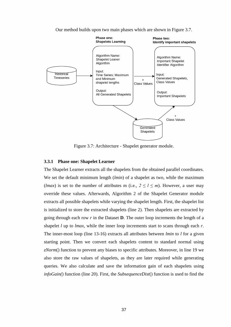
Our method builds upon two main phases which are shown in Figure 3.7.

Figure 3.7: Architecture - Shapelet generator module.

3.3.1 Phase one: Shapelet Learner

The Shapelet Learner extracts all the shapelets from the obtained parallel coordinates.

We set the default minimum length (lmin) of a shapelet as two, while the maximum

(lmax) is set to the number of attributes m (i.e., 2 ≤ l ≤ m). However, a user may

override these values. Afterwards, Algorithm 2 of the Shapelet Generator module

extracts all possible shapelets while varying the shapelet length. First, the shapelet list

is initialized to store the extracted shapelets (line 2). Then shapelets are extracted by

going through each row r in the Dataset D. The outer loop increments the length of a

shapelet l up to lmax, while the inner loop increments start to scans through each r.

The inner-most loop (line 13-16) extracts all attributes between lmin to l for a given

starting point. Then we convert each shapelets content to standard normal using

zNorm() function to prevent any biases to specific attributes. Moreover, in line 19 we

also store the raw values of shapelets, as they are later required while generating

queries. We also calculate and save the information gain of each shapelets using

infoGain() function (line 20). First, the SubsequenceDist() function is used to find the

38

minimum distance between the row and the shapelet by sliding the shapelet across the

row, one attribute at a time (see Figure 3.6). By repeating the function, the minimum

distance per each row is found and saved in an array. Then by sequentially splitting

the array we calculate the information gain using Eq. 2. Finally, for each shapelet we

get the maximum information gain and the corresponding split point, which would be

the Optimum Splitting Point of the array. In line 21, each shapelet and its metadata are

then added to the shapelets list, which is later returned by the algorithm.

Algorithm 3.2: Shapelet learner algorithm.

All possible shapelets will be extracted from a given dataset. In addition to the

Algorithm 3.2 the dataset will be standardized in to a normal distribution and based on

39

that shapelets will be extracted. Extracted shapelets can be saved into a database or

simply use as the input for the second phase.

3.3.2 Phase two Shapelet Extraction

All the extracted shapelets are first sorted according to their information gain. Then

these shapelets are divided into a set of groups and then merged using Algorithm 3.3.

Algorithm takes the set of shapelets S and number of shapelets per group (groupsize)

as the input. groupsize is selected based on the cluster pruning technique in which we

set the number of groups to the square root of the total number of identified shapelets.

If desired, the user may also define the groupsize. Then in line 12 to 15 the grouped

shapelets are updated by adding their series ID (i.e., row number), starting positions

(i.e., starting attribute index), and class value (i.e., event type). Finally, the algorithm

return all the merged shapelets (line 25).

40

Algorithm 3.3: Shapelet merger algorithm.

Important Shapelet Finder algorithm (Algorithm 3.4) takes in three parameters, namely

merged shapelets, classified/labelled dataset and class values (i.e., event types). Line

2 and 3 initialize two lists named shapeletArr and classValueProb, which would

respectively contain important shapelets and probabilities for class values within the

total dataset. Then for each class value, a set data structure is created named

shapeletBucket. findProb() function calculates the probability of the relevant class

values within the dataset, and then put that to shapeletBucket (line 8 to 10). As the next

step, (in line 12 to 17) each merged shapelet is included into a relevant shapeletBucket,

based on the most probable class values for each group of shapelets. This is achieved

using maxProbClassVal() function. Next, Algorithm 3.4 finds the absolute differences

between the probabilities of actual events of the dataset and groups of shapelets. This

is calculated using the getMinDifShape() function (line 28). Because the chosen group

of shapelets per each event comprises of the minimum difference with respect to the

actual event distribution in the dataset, it enables us to choose the most representative

groups of shapelets per each event. Finally, the extracted group of shapelets are added

to the shapeletArr (line 29).

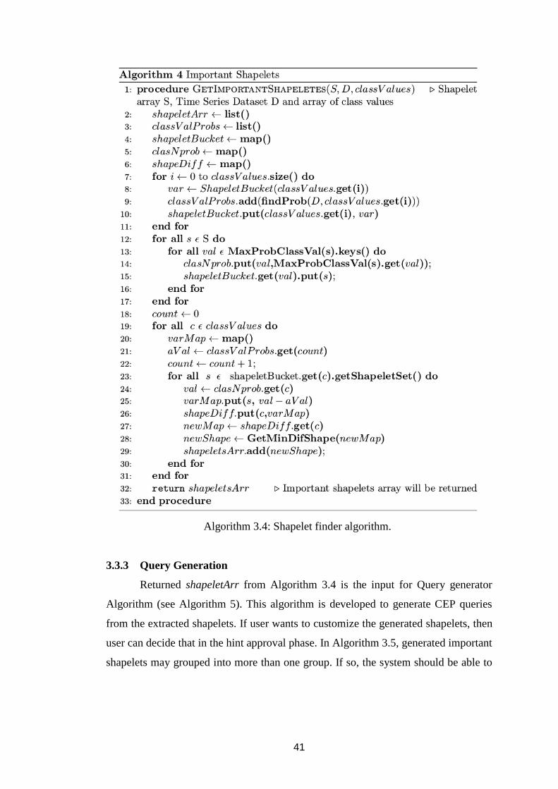
41

Algorithm 3.4: Shapelet finder algorithm.

3.3.3 Query Generation

Returned shapeletArr from Algorithm 3.4 is the input for Query generator

Algorithm (see Algorithm 5). This algorithm is developed to generate CEP queries

from the extracted shapelets. If user wants to customize the generated shapelets, then

user can decide that in the hint approval phase. In Algorithm 3.5, generated important

shapelets may grouped into more than one group. If so, the system should be able to

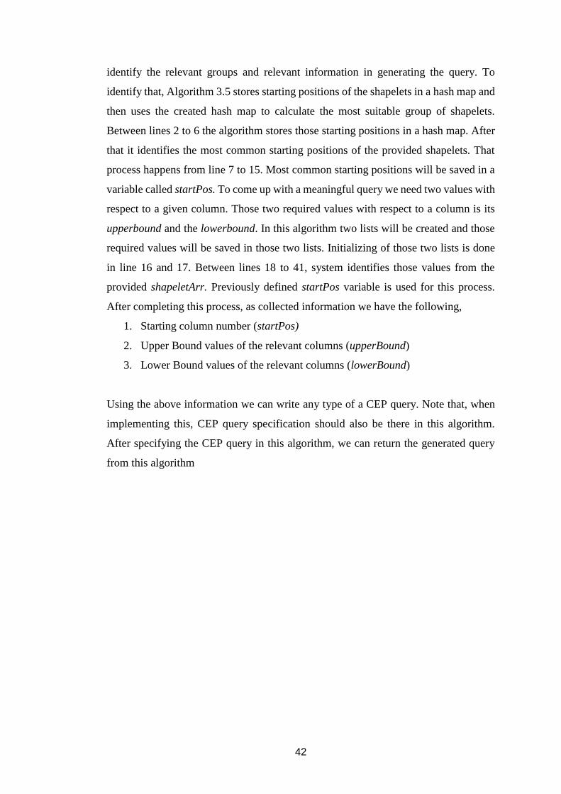
42

identify the relevant groups and relevant information in generating the query. To

identify that, Algorithm 3.5 stores starting positions of the shapelets in a hash map and

then uses the created hash map to calculate the most suitable group of shapelets.

Between lines 2 to 6 the algorithm stores those starting positions in a hash map. After

that it identifies the most common starting positions of the provided shapelets. That

process happens from line 7 to 15. Most common starting positions will be saved in a

variable called startPos. To come up with a meaningful query we need two values with

respect to a given column. Those two required values with respect to a column is its

upperbound and the lowerbound. In this algorithm two lists will be created and those

required values will be saved in those two lists. Initializing of those two lists is done

in line 16 and 17. Between lines 18 to 41, system identifies those values from the

provided shapeletArr. Previously defined startPos variable is used for this process.

After completing this process, as collected information we have the following,

1. Starting column number (startPos)

2. Upper Bound values of the relevant columns (upperBound)

3. Lower Bound values of the relevant columns (lowerBound)

Using the above information we can write any type of a CEP query. Note that, when

implementing this, CEP query specification should also be there in this algorithm.

After specifying the CEP query in this algorithm, we can return the generated query

from this algorithm

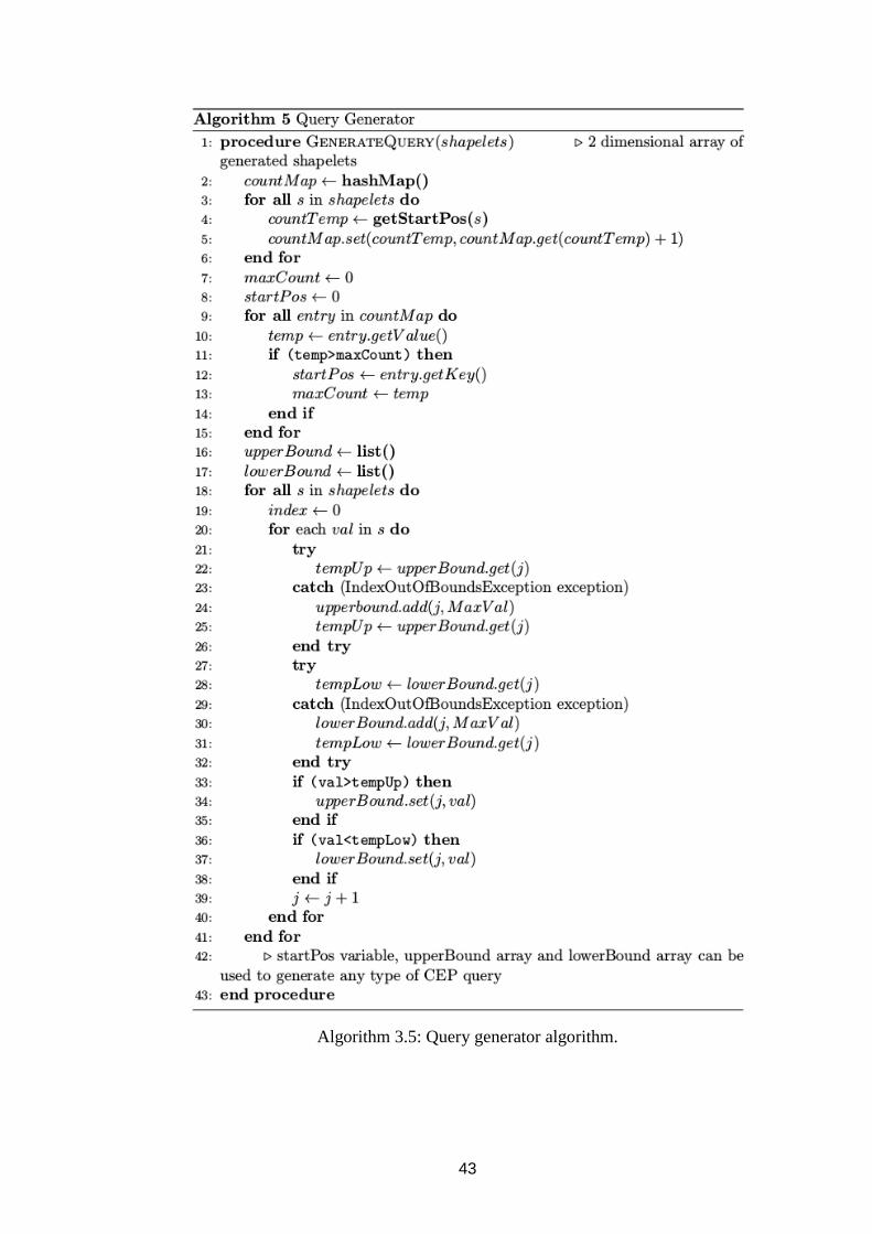
43

Algorithm 3.5: Query generator algorithm.

44

Chapter 4

IMPLEMENTATION AND PERFORMANCE EVALUATION

We implemented a web application to visualize the project output to the user. This web

application demonstrate the full life cycle of automated query generation. Section 4.1

describes the development framework. The features of the web application are

presented in Section 4.2. Section 4.3 illustrates the data visualization of the application

and performance evaluation is presented in Section 4.4.

4.1 Web Application with spring

SPRING Framework has been used for this development and the resulted shapelets

will be appeared to the user as set of graphs [27]. Then user can customize the

generated results and proceed to create a query for the respective events.

The reasons of selecting spring framework for our development are as follows:

1. Spring provides a very clean division between controllers, JavaBean models,

and views. Here the complete application has been divided into three main

components.

a. Model - Model is where the application’s data objects are stored. The

model does not know anything about views and controllers. When a

model changes, typically it will notify its observers that a change has

occurred.

b. View - View is what is presented to the users and how users interact

with the app. The view is made with HTML, CSS, JavaScript and often

templates.

c. Controller - The controller is the decision maker and the glue between

the model and view. The controller updates the view when the model

changes. It also adds event listeners to the view and updates the model

when the user manipulates the view.

2. Spring MVC is truly view-agnostic. You do not get pushed to use JSP if you

do not want to; you can use Velocity, XLST or other view technologies. If you

want to use a custom view mechanism

45

3. Spring comes with various design patterns in its core principles

4. Provides dependency injection.

4.2 Features of Web Application

This web application provides following set of APIs:

1. Uploading a dataset

API can be used to upload datasets to the system. Any supported dataset (CSV

of ARFF can be uploaded using this API. If there is an annotated dataset user

can specify it to proceed directly to the Shapelet Generator module, otherwise

dataset can be annotated by Data Processor module with user request. A HTTP

POST request should be sent to the API with the Multipart File attached.

2. Get uploaded datasets

All the uploaded files will be saved in the system for reuse. A HTTP GET

request should be sent to the API and it will send back a JSON file containing

all the details of the uploaded datasets.

3. Start generating shapelets

A HTTP GET request should be sent to the API with Email and Dataset name

attached as parameters. Here Spring Asynchronous task will be initiated. Since

this process may take some time to complete, an email will be sent to the

provided email address with a url once the process completed. Websockets are

used to notify the frontend once the generating shapelets is completed. In

summary there are two ways to notify the user once the processing is

completed.

a. Email notification [28].

b. Notification on frontend [29].

4. Get generated shapelets by simply sending a HTTP GET request to this API

with dataset name attached as a parameter, generated shapelets files can be

retrieved. A simple JSON file will be returned.

5. Generate queries - This API can be used to generate the queries for most

important shapelets generated by the system. Dataset name has to be sent as a

parameter and a JSON file containing all the queries will be returned.

46

After generating shapelets, we generate a JSON file including all the details of

generated shapelets such as no of events, event type, content values for each content

etc. Then this JSON file was used to draw graphs. Since we have to get user

involvement on graphs we tried different APIs which supports our requirement.

Google Chart, ChartJS are two APIs and D3 is a library which supports dynamic

visualizations on web browsers. Out of these we chose ChartJS which is the best

solution for our scenario to customize graphs.

4.3 Screenshots of Web Application

4.3.1 Home Page

Homepage enables user to upload data files to the server, here the file type should be .csv or

.arff. Even user can upload multiple files to the server for later usages. After getting uploaded

files to the server user can start the process in the shapelet generator module by selecting a

uploaded dataset and providing an valid email address. This email address will get an email

after completing the process in the server.

Figure 4.1: Home page of Web application.

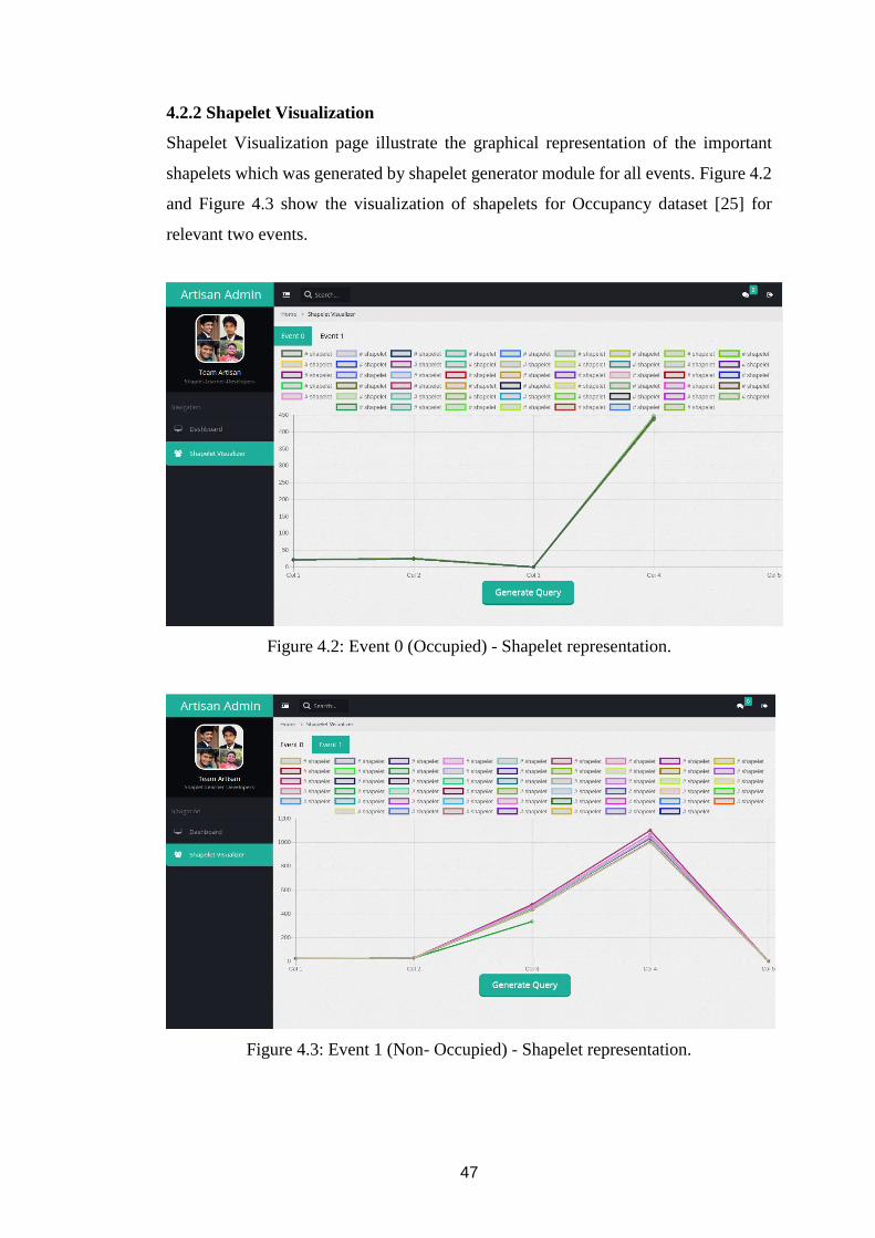
47

4.2.2 Shapelet Visualization

Shapelet Visualization page illustrate the graphical representation of the important

shapelets which was generated by shapelet generator module for all events. Figure 4.2

and Figure 4.3 show the visualization of shapelets for Occupancy dataset [25] for

relevant two events.

Figure 4.2: Event 0 (Occupied) - Shapelet representation.

Figure 4.3: Event 1 (Non- Occupied) - Shapelet representation.

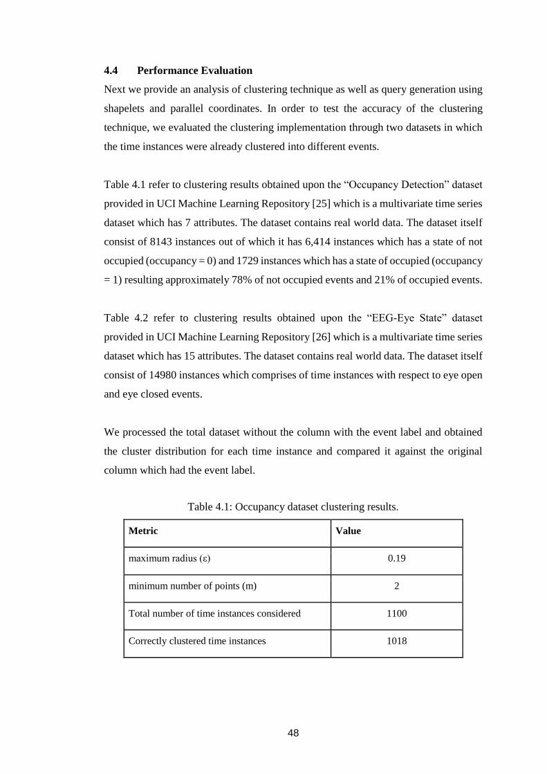
48

4.4 Performance Evaluation

Next we provide an analysis of clustering technique as well as query generation using

shapelets and parallel coordinates. In order to test the accuracy of the clustering

technique, we evaluated the clustering implementation through two datasets in which

the time instances were already clustered into different events.

Table 4.1 refer to clustering results obtained upon the “Occupancy Detection” dataset

provided in UCI Machine Learning Repository [25] which is a multivariate time series

dataset which has 7 attributes. The dataset contains real world data. The dataset itself

consist of 8143 instances out of which it has 6,414 instances which has a state of not

occupied (occupancy = 0) and 1729 instances which has a state of occupied (occupancy

= 1) resulting approximately 78% of not occupied events and 21% of occupied events.

Table 4.2 refer to clustering results obtained upon the “EEG-Eye State” dataset

provided in UCI Machine Learning Repository [26] which is a multivariate time series

dataset which has 15 attributes. The dataset contains real world data. The dataset itself

consist of 14980 instances which comprises of time instances with respect to eye open

and eye closed events.

We processed the total dataset without the column with the event label and obtained

the cluster distribution for each time instance and compared it against the original

column which had the event label.

Table 4.1: Occupancy dataset clustering results.

Metric Value

maximum radius (ε) 0.19

minimum number of points (m) 2

Total number of time instances considered 1100

Correctly clustered time instances 1018

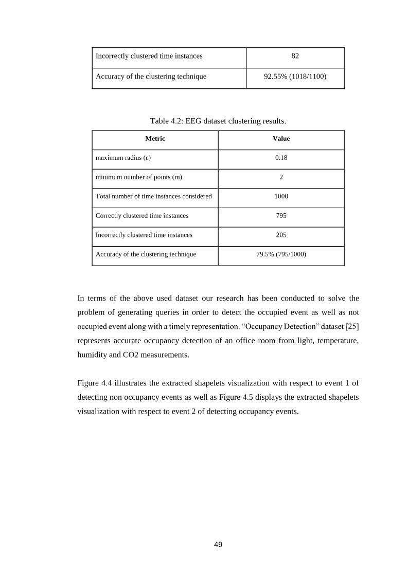
49

Incorrectly clustered time instances 82

Accuracy of the clustering technique 92.55% (1018/1100)

Table 4.2: EEG dataset clustering results.

Metric Value

maximum radius (ε) 0.18

minimum number of points (m) 2

Total number of time instances considered 1000

Correctly clustered time instances 795

Incorrectly clustered time instances 205

Accuracy of the clustering technique 79.5% (795/1000)

In terms of the above used dataset our research has been conducted to solve the

problem of generating queries in order to detect the occupied event as well as not

occupied event along with a timely representation. “Occupancy Detection” dataset [25]

represents accurate occupancy detection of an office room from light, temperature,

humidity and CO2 measurements.

Figure 4.4 illustrates the extracted shapelets visualization with respect to event 1 of

detecting non occupancy events as well as Figure 4.5 displays the extracted shapelets

visualization with respect to event 2 of detecting occupancy events.

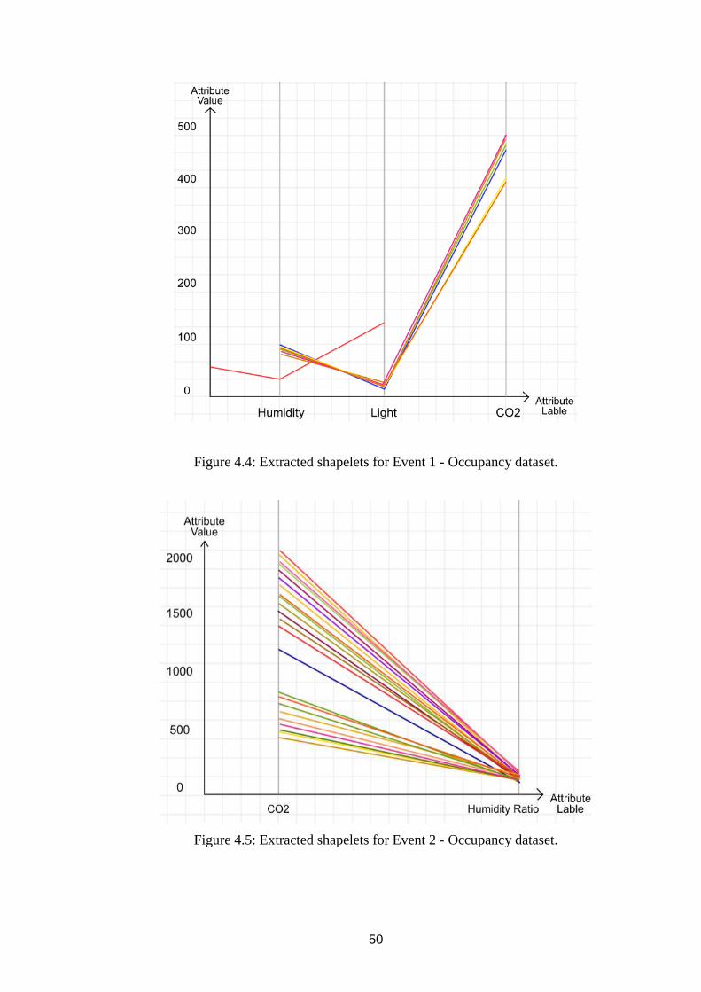
50

Figure 4.4: Extracted shapelets for Event 1 - Occupancy dataset.

Figure 4.5: Extracted shapelets for Event 2 - Occupancy dataset.

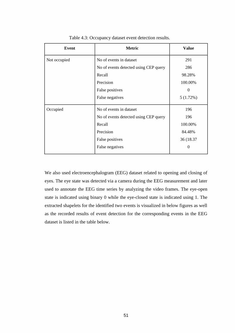
51

Table 4.3: Occupancy dataset event detection results.

Event Metric Value

Not occupied No of events in dataset

No of events detected using CEP query

Recall

Precision

False positives

False negatives

291

286

98.28%

100.00%

0

5 (1.72%)

Occupied No of events in dataset

No of events detected using CEP query

Recall

Precision

False positives

False negatives

196

196

100.00%

84.48%

36 (18.37

0

We also used electroencephalogram (EEG) dataset related to opening and closing of

eyes. The eye state was detected via a camera during the EEG measurement and later

used to annotate the EEG time series by analyzing the video frames. The eye-open

state is indicated using binary 0 while the eye-closed state is indicated using 1. The

extracted shapelets for the identified two events is visualized in below figures as well

as the recorded results of event detection for the corresponding events in the EEG

dataset is listed in the table below.

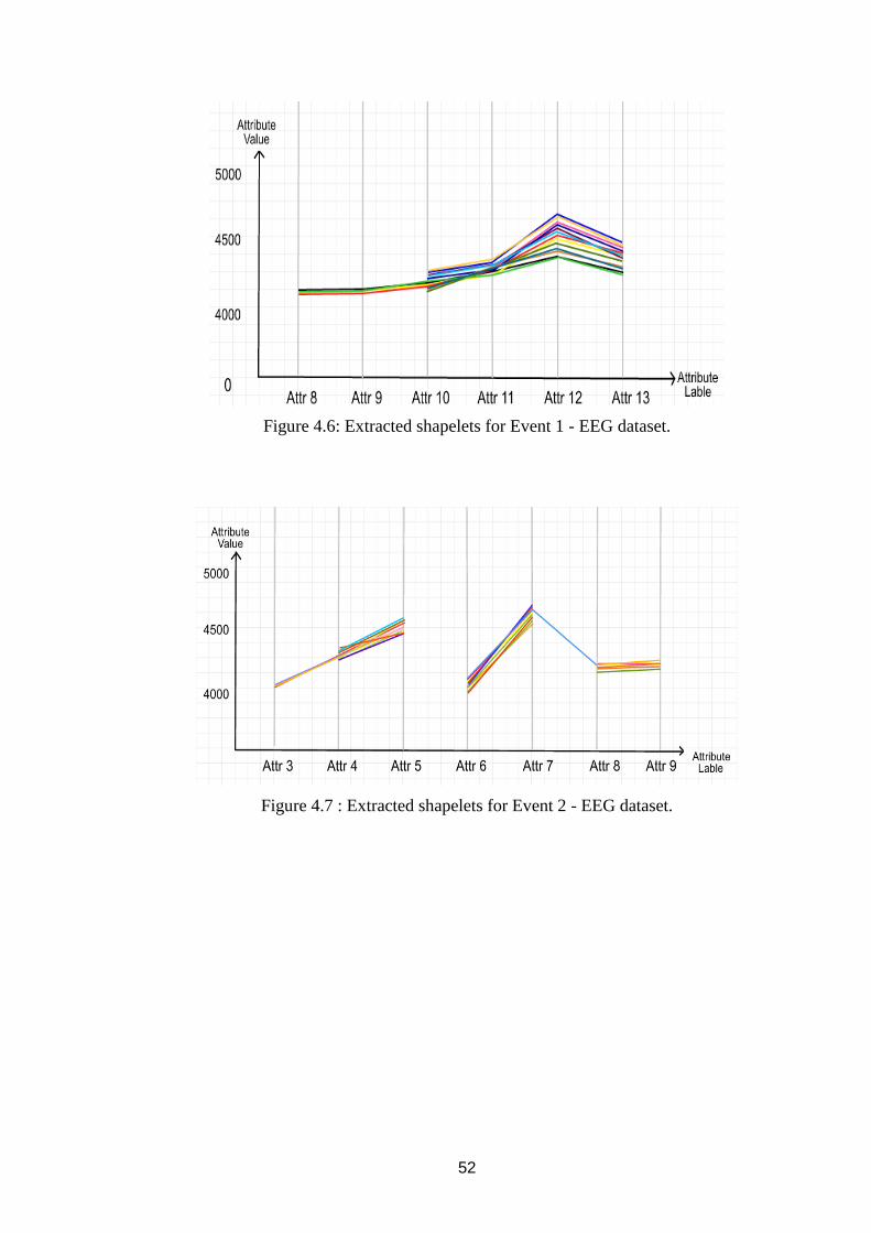
52

Figure 4.6: Extracted shapelets for Event 1 - EEG dataset.

Figure 4.7 : Extracted shapelets for Event 2 - EEG dataset.

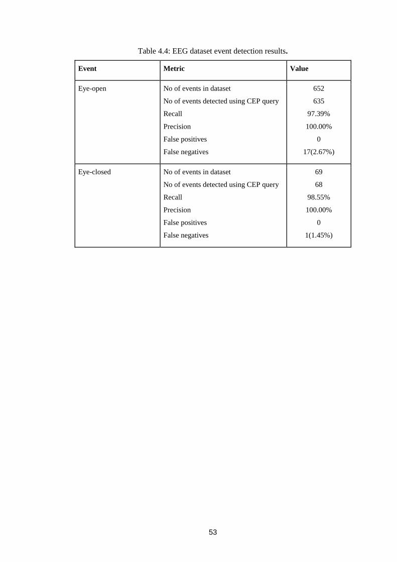
53

Table 4.4: EEG dataset event detection results.

Event Metric Value

Eye-open No of events in dataset

No of events detected using CEP query

Recall

Precision

False positives

False negatives

652

635

97.39%

100.00%

0

17(2.67%)

Eye-closed No of events in dataset

No of events detected using CEP query

Recall

Precision

False positives

False negatives

69

68

98.55%

100.00%

0

1(1.45%)

54

Chapter 5

SUMMARY

5.1 Conclusion

Complex Event Processing (CEP) combines data from multiple sources to detect

events or patterns that suggest much more complicated circumstances. Modern day

CEP engines are used across many domains and applications with the objective of

identifying meaningful events in near real time. For example, CEP is effectively used

in the financial domains such as stock markets and credit card fraud detection

Accuracy of the output of CEP depends on the queries that are used to process the data.

However, it is not straightforward to write CEP queries, as they depend on many

attributes of the event being monitored and their correlations. Moreover, significant

insight is required to write effective queries; hence the the query generation process is

domain and user dependent. Automated CEP query generation is identified as one of

the promising alternatives, and several prior work address different aspects of the

problem. However, existing techniques are computationally expensive, works only for

univariate data, and require extensive domain-specific human interaction.

We looked into this issue of providing a domain and user independent solution for the

automated query generation for CEP. We proposed technique to automatically

generate CEP queries based on multivariate time series data. The proposed technique

first map the multivariate time series to a set of parallel coordinates. Then key patterns

that are representative of the events are identified using time series shapelets. We also

propose a technique to identify the most relevant shapeless per event, such that only a

single CEP query will be generated per event. This enables one to generate CEP

queries for commonalities, anomalies, as well as time-series breakpoints in a given

multivariate time-series dataset without having any domain knowledge. Users can

focus on groups with high or low information gain depending on the application.

Furthermore, for datasets that are not pre-annotated, we proposed a technique to label

the data by clustering the dataset into a set of clusters based on similarity (measured

using Euclidean distance) between time instances. This produces a labeled dataset in

which each time instance is labeled with the respective event it belongs to.

55

The proposed technique is both computationally and memory efficient compared to

prior work, as the length of a shapelet is bounded by the number of attributes.

Moreover, the performance of the CEP engine is also improved, as only one query will

be generated per events. The proposed technique can be applied to both multivariate

and multivariate time-series data regardless of the domain, and it is computationally

and memory efficient. Using two real datasets, we demonstrate that the resulting

queries have good accuracy in detecting relevant events. Our approach remarks its

importance due to its nature of user and domain independence, as well as producing

high accuracies and precision with respect to the experimental results. Furthermore,

the developed tool enables if a domain expert users interacts with our system and use,

our approach facilitates to that user also by allowing the user to provide insights in

order to optimize and change the query generation process to his or her likeness.

5.2 Future Work

The current implementation does not facilitate constructing CEP queries while

capturing interdependencies among attributes in multivariate time series. For example,

on a server CPU fan speed is correlated to the CPU utilization. However, as the CPU

utilization increases, fan speed does not increase immediately. It will increase the

speed only after sometime. Similarly, fan speed does not reduce as soon as CPU

utilization goes down. The proposed technique cannot write accurate window-based

queries for such instances. Figuring out such interdependencies among the attributes

would be useful to generate more accurate and complex queries.

While the proposed clustering-based technique is effective in annotating time series

datasets with events, it accuracy need to be further improved. Similarly, between two

time series instances cannot capture complex relationships among data points. For

example, the CPU utilization and fan speed example could be interpreted as two

independent events by our clustering solution. Hence, further work is required in this

area. Moreover, due to curse of dimensionality Euclidean distance based similarity

measure becomes less effective as the number of attributes increase.

56

In terms of the web interface the limitation exists in obtaining user insights provided

that the user needs to interact with the systems. Here the main issue lies within the

difficulty of allowing user to select the ranges of the most important shapelets that are

been generated from the system in order to build up the CEP query.

57

References

[1] G. Cugola, A. Margara and G. Tamburrelli, “Towards automated rule learning for

complex event processing,” Tech. Rep., 2013.

[2] A. Margara, G. Cugola, and G. Tamburrelli, “Learning from the past,” pp. 47–58,

May 2014. [Online]. Available: http://dl.acm.org/citation.cfm?id=2611289.

[3] R. Mousheimish, Y. Taher, and K. Zeitouni, “Complex event processing for the

non-expert with autoCEP,” pp. 340–343, Jun. 2016. [Online]. Available:

http://dl.acm.org/citation.cfm?id=2933296. Accessed: Jul. 24, 2016.

[4]M. Wistuba, J. Grabocka, and L. Schmidt-Thieme, "Ultra-fast Shapelets for time

series classification,".

[5] R.N. Navagamuwa, K.J.P.G. Perera, M.R.M.J. Sally,L.A.V.N. Prashan, and

H.M.N.D. Bandara, “Shapelets and Parallel Coordinates Based Automated Query

Generation for Complex Event Processing,” in Proc. 2016 IEEE Intl. Conf. on Smart

Data (SmartData ‘16), Chengdu, China, Dec. 2016, pp. 846-853..

[6] G. Cugola, A. Margara, M. Matteucci, and G. Tamburrelli, “Introducing

uncertainty in complex event processing: Model, implementation, and validation,”

Computing, pages 1–42, 2014.

[7] H. Obweger, J. Schiefer, M. Suntinger, P. Kepplinger, and S. Rozsnyai, “User-

oriented rule management for event-based applications,” pp. 39–48, Nov. 2011.

[8] A. Kavelar, H. Obweger, J. Schiefer, and M. Suntinger, “Web-based decision

making for complex event processing systems,” pp. 453–458, Jul. 2010.

[9] Y. Turchin, A. Gal, and S. Wasserkrug, “Tuning complex event processing rules

using the prediction-correction paradigm,” p. 10, Jun. 2009.

[10] S. Sen, N. Stojanovic, and L. Stojanovic, “An approach for iterative event pattern

recommendation,” pp. 196–205, Dec. 2010. [Online]. Available:

http://dl.acm.org/citation.cfm?id=1827459.

58

[11] M. Philippsen and C.Mutschler, “Learning Event Detection Rules with Noise

Hidden Markov Models,” in Proc. 2012 NASA/ESA Conference on Adaptive

Hardware and Systems (AHS-2012), 2012.

[12] E. Alevizos, A. Skarlatidis, A. Artikis, and G. Paliouras, "Complex event

recognition under uncertainty: A short survey," in EDBT/ICDT 2015, Brussels,

Belgium, 2015. [Online]. Available: http://ceur-ws.org/Vol-1330/paper-18.pdf.

[13] R. Kalman. A new approach to linear filtering and prediction problems. Journal

of Basic Engineering, vol. 82, no. 1pp. 35–45, 1960.

[14] "Complex Event Processor", Wso2.com, 2017. [Online]. Available:

http://wso2.com/products/complex-event-processor/.

[15] V. Cristea, F. Pop, C. Dobre, and A. Costan, “Distributed architectures for event-

based systems,” in Proc. Reasoning in Event-Based Distributed Systems. Springer

Science + Business Media, 2011, pp. 11–45.

[16]2016,"Products-

Esper,"2006.[Online].Available:http://www.espertech.com/products/esper.php.

[17]F. Fournier, A. Kofman, I. Skarbovsky, and A. Skarlatidis, "Extending event-

driven architecture for Proactive systems," Brussels, Belgium, Mar. 27, 2015. [Online].

Available: http://ceur-ws.org/Vol-1330/paper-19.pdf.

[18] J. Johansson and C. Forsell, “Evaluation of parallel coordinates: Overview,

categorization and guidelines for future research,” IEEE Trans. Vis. Comput.

Graphics, vol. 22, pp. 579–588, 2016.

[19] S. Wasserkrug, A. Gal, O. Etzion, and Y. Turchin, “Efficient processing of

uncertain events in rule-based systems,” IEEE Transactions on Knowledge and Data

Engineering, vol. 24, no. 1, pp. 45–58, Jan. 2012.

[20]L. J. Fülöp, Á. Beszédes, G. Tóth, H. Demeter, L. Vidács, and L. Farkas,

"Predictive complex event processing," Proceedings of the Fifth Balkan Conference in

59

Informatics on - BCI’12,2012.[Online].Available:http://www.inf.u-

szeged.hu/~beszedes/research/bci2012_submission_41_camera_ready.pdf.

[21] L. Ye and E. Keogh, “Time series shapelets,” pp. 947–956, Jun. 2009. [Online].

Available: http://dl.acm.org/citation.cfm?id=1557122. Accessed: Aug. 7, 2016.

[22] P. Gay, B. López, and J. Meléndez, “Sequential learning for case-based pattern

recognition in complex event domains,”

[23] O. P. Patri, A. B. Sharma, H. Chen, G. Jiang, A. V. Panangadan, and V. K.

Prasanna, “Extracting discriminative shapelets from heterogeneous sensor data,” in

Proc. 2014 IEEE Intl. Conf. on Big Data (Big Data), 2014

[24]“Clustering-hierarchical,”1967.[Online].

Available:https://home.deib.polimi.it/matteucc/Clustering/tutorial_html/hierarchical.

html

[25] R. Feldheim, “UCI machine learning repository: Occupancy detection data set,”

2016. [Online]. Available:

https://archive.ics.uci.edu/ml/datasets/Occupancy+Detection+.

[26] "UCI machine learning repository: EEG eye state data set," 2013. [Online].

Available: https://archive.ics.uci.edu/ml/datasets/EEG+Eye+State

[27] “SPRING documentation,”. [Online]. Available: https://spring.io/docs

[28] “STOMP over websocket,”. [Online]. Available: http://jmesnil.net/stomp-

websocket/doc/

[29] “SendGrid email api documentation,”. [Online]. Available:

https://sendgrid.com/docs/API_Reference/Web_API_v3/index.html

[30] M. Bostock, “D3.js - data-driven documents,”. [Online]. Available:

https://d3js.org/

[31] M. Ankerst, M. M. Breunig, H. Kriegel, and J. Sander, “OPTICS: Ordering Points

To Identify the Clustering Structure”, in Proc/ ACM SIGMOD’99 Intl. Conf. on

Management of Data, Philadelphia, 1999.

60

[32] H. Backlund, A. Hedblom, N. Neijman, “A density-based spatial clustering of

application with noise”, 2011

[33] C. Jin, M. M. A. Patwary, A. Agrawal, W. Hendrix, W. Liao, and A. Choudhary,

“Disc: A distributed single-linkage hierarchical clustering algorithm using

MapReduce”, in Proc. 4th Intl. SC Workshop on Data Intensive Computing in the

Clouds (DataCloud), 2013.

61

Appendix A: Accepted paper for IEEE International Conference

on Smart Data 2016

2016 IEEE International Conference on Internet of Things (iThings) and IEEE Green Computing and

Communications (GreenCom) and IEEE Cyber, Physical and Social Computing (CPSCom) and IEEE

Smart Data (SmartData)

Shapelets and Parallel Coordinates Based Automated Query

Generation for Complex Event Processing

R.N. Navagamuwa, K.J.P.G. Perera, M.R.M.J. Sally, L.A.V.N. Prashan, and H.M.N. Dilum Bandara

Department of Computer Science and Engineering

University Of Moratuwa

Katubedda, Sri Lanka

Email: (randika.12, pravinda.12, jaward.12, prashan.12, dilumb)@cse.mrt.ac.lk

Abstract—Automating the query generation for

Complex Event Processing (CEP) has marked its own

importance in allowing users to obtain useful insights

from data. Existing techniques are both

computationally expensive and require extensive

domainspecific human interaction. In addressing these

issues, we propose a technique that combines both

parallel coordinates and shapelets. First, each instance

of the multivariate data is represented as a line on a set

of parallel coordinates. Then a shapelet-learner

algorithm is applied to those lines to extract the

relevant shapelets. Afterwards, the identified shapelets

are ranked based on their information gain. Next, the

shapelets with similar information gain are divided into

groups by a shapeletmerger algorithm. The best group

for each event is then identified based on the event

distribution of the dataset. Then the best group is used

to generate the query to detect the complex events.

The proposed technique can be applied to both

multivariate and multivariate time-series data, and it is

computationally and memory efficient. It enables users

to focus only on the shapelets with relevant

information gains. We demonstrate the utility of the

proposed technique using a set of real-world datasets.

Index Terms—Complex Event Processing,

Multivariate Time Series, Parallel Coordinates,

Shapelets

I. INTRODUCTION

Automating query generation in large, multivariate datasets

are useful in many application domains. For example,

Complex Event Processing (CEP) [1] combines data from

multiple, streaming sources to identify meaningful events or

patterns in real time. While the detection of relevant events

and patterns may give insight about opportunities and

threats related to the data being monitored (e.g., a set of

sensor readings and credit card transactions), significant

domain knowledge is required to write effective CEP

queries. Manual analysis of data streams is not only tedious

and error prone, but also important events are likely to be

missed due to the limited domain knowledge of the query

writer. A promising alternative is to automate the CEP

query generation by automatically extracting/mining

interesting patterns from the past data [2], [3], [4].

Time-series pattern mining and classification

techniques are extensively studied in the literature.

Dynamic Time Warping (DTW) [5] is one such technique

used to measure the similarity between two time-series

based on a distance measure. However, the computational

complexity of DTW grows exponentially with large and

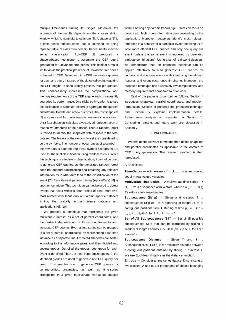
62

multiple time-series limiting its usages. Moreover, the

accuracy of the results depends on the chosen sliding

window, which is nontrivial to estimate [2]. A shapelet [6] is

a time series subsequence that is identified as being

representative of class membership; hence, useful in time-

series classification. AutoCEP [2] proposed a

shapeletbased technique to automate the CEP query

generation for univariate time series. This itself is a major

limitation as the practical presence of univariate time series

is limited in CEP. Moreover, AutoCEP generates queries

for each and every instance of the detected event, requiring

the CEP engine to concurrently process multiple queries.

This unnecessarily increases the computational and

memory requirements of the CEP engine and consequently

degrades its performance. One trivial optimization is to use

the assistance of a domain-expert to aggregate the queries

and attempt to write one or few queries. Ultra-fast shapelets

[7] are proposed for multivariate time-series classification.

Ultra-fast shapelets calculate a vectorized representation of

respective attributes of the dataset. Then a random forest

is trained to identify the shapelets with respect to the total

dataset. The leaves of the random forest are considered to

be the symbols. The number of occurrences of a symbol in

the raw data is counted and these symbol histograms are

used for the final classification using random forests. While

this technique is effective in classification, it cannot be used

to generate CEP queries, as the generated random forest

does not support backtracking and obtaining any relevant

information as to what data lead to the classification of the

event [7]. Rare itemset pattern mining (AprioriRare) [8] is

another technique. This technique cannot be used to detect

events that occur within a short period of time. Moreover,

most related work focus only on domain-specific datasets

limiting the usability across diverse datasets and

applications [9], [10].

We propose a technique that represents the given

multivariate dataset as a set of parallel coordinates, and

then extract shapelets out of those coordinates to auto

generate CEP queries. Even a time series can be mapped

to a set of parallel coordinates, by representing each time

instance as a separate line. Extracted shapelets are sorted

according to the information gains and then divided into

several groups. Out of all the groups, best group for each

event is identified. Then the most important shapelets in the

identified groups are used to generate one CEP query per

group. This enables one to generate CEP queries for

commonalities, anomalies, as well as time-series

breakpoints in a given multivariate time-series dataset

without having any domain knowledge. Users can focus on

groups with high or low information gain depending on the

application. Moreover, shapelets identify most relevant

attributes in a dataset for a particular event, enabling us to

write more efficient CEP queries and only one query per

event (unless the same event is triggered by unrelated

attribute combinations). Using a set of real-world datasets,

we demonstrate that the proposed technique can be

applied effectively to auto generate CEP queries for

common and abnormal events while identifying the relevant

features and event occurrence timeframe. Moreover, the

proposed technique has a relatively low computational and

memory requirements compared to prior work.

Rest of the paper is organized as follows. Section II

introduces shapelets, parallel coordinates, and problem

formulation. Section III presents the proposed technique

and Section IV explains implementation details.

Performance analysis is presented in Section V.

Concluding remarks and future work are discussed in

Section VI.

II. PRELIMINARIES

We first define relevant terms and then define shapelets

and parallel coordinates as applicable to the domain of

CEP query generation. The research problem is then

formulated.

A. Definitions

Time-Series — A time-series T = t1, ..., tm is an ordered

set of m real-valued variables.

Multivariate Time-Series — A multivariate time-series T =

t1, ..., tm is a sequence of m vectors, where ti = (ti,1, ..., ti,s)

Rs with s attributes/variables.

Sub-sequence (St p) — Given a time-series T, a

subsequence St p of T is a sampling of length l ≤ m of

contiguous positions from T starting at time p, i.e., St p =

tp, tp+1..., tp+l−1, for 1 ≤ p ≤ m − l + 1.

Set of All Sub-sequences (STl) — Set of all possible

subsequences St p that can be extracted by sliding a

window of length l across T is STl = {all St p of T, for 1 ≤ p

≤ m−l+1}.

Sub-sequence Distance — Given T and St p

SubsequenceDist(T,St p) is the minimum distance between

p contiguous positions obtained by sliding St p across T.

We use Euclidean distance as the distance function.

Entropy — Consider a time series dataset D consisting of

two classes, A and B. Let proportions of objects belonging

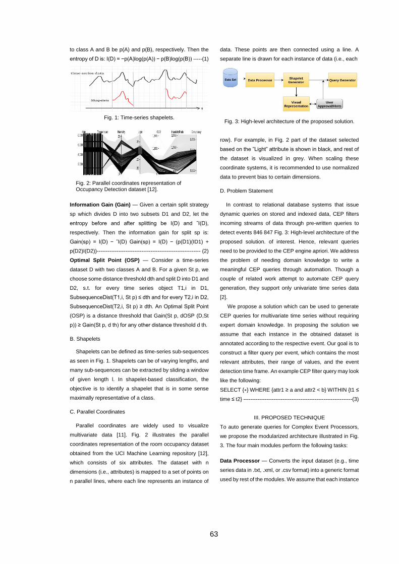
63

to class A and B be p(A) and p(B), respectively. Then the

entropy of D is: I(D) = −p(A)log(p(A)) − p(B)log(p(B)) -----(1)

Fig. 1: Time-series shapelets.

Fig. 2: Parallel coordinates representation of Occupancy Detection dataset [12].

Information Gain (Gain) — Given a certain split strategy

sp which divides D into two subsets D1 and D2, let the

entropy before and after splitting be I(D) and ˆI(D),

respectively. Then the information gain for split sp is:

Gain(sp) = I(D) − ˆI(D) Gain(sp) = I(D) − (p(D1)(ID1) +

p(D2)I(D2))---------------------------------------------------------- (2)

Optimal Split Point (OSP) — Consider a time-series

dataset D with two classes A and B. For a given St p, we

choose some distance threshold dth and split D into D1 and

D2, s.t. for every time series object T1,i in D1,

SubsequenceDist(T1,i, St p) ≤ dth and for every T2,i in D2,

SubsequenceDist(T2,i, St p) ≥ dth. An Optimal Split Point

(OSP) is a distance threshold that Gain(St p, dOSP (D,St

p)) ≥ Gain(St p, d th) for any other distance threshold d th.

B. Shapelets

Shapelets can be defined as time-series sub-sequences

as seen in Fig. 1. Shapelets can be of varying lengths, and

many sub-sequences can be extracted by sliding a window

of given length l. In shapelet-based classification, the

objective is to identify a shapelet that is in some sense

maximally representative of a class.

C. Parallel Coordinates

Parallel coordinates are widely used to visualize

multivariate data [11]. Fig. 2 illustrates the parallel

coordinates representation of the room occupancy dataset

obtained from the UCI Machine Learning repository [12],

which consists of six attributes. The dataset with n

dimensions (i.e., attributes) is mapped to a set of points on

n parallel lines, where each line represents an instance of

data. These points are then connected using a line. A

separate line is drawn for each instance of data (i.e., each

Fig. 3: High-level architecture of the proposed solution.

row). For example, in Fig. 2 part of the dataset selected

based on the ”Light” attribute is shown in black, and rest of

the dataset is visualized in grey. When scaling these

coordinate systems, it is recommended to use normalized

data to prevent bias to certain dimensions.

D. Problem Statement

In contrast to relational database systems that issue

dynamic queries on stored and indexed data, CEP filters

incoming streams of data through pre-written queries to

detect events 846 847 Fig. 3: High-level architecture of the

proposed solution. of interest. Hence, relevant queries

need to be provided to the CEP engine apriori. We address

the problem of needing domain knowledge to write a

meaningful CEP queries through automation. Though a

couple of related work attempt to automate CEP query

generation, they support only univariate time series data

[2].

We propose a solution which can be used to generate

CEP queries for multivariate time series without requiring

expert domain knowledge. In proposing the solution we

assume that each instance in the obtained dataset is

annotated according to the respective event. Our goal is to

construct a filter query per event, which contains the most

relevant attributes, their range of values, and the event

detection time frame. An example CEP filter query may look

like the following:

SELECT {∗} WHERE {attr1 ≥ a and attr2 < b} WITHIN {t1 ≤

time ≤ t2} -------------------------------------------------------------(3)

III. PROPOSED TECHNIQUE

To auto generate queries for Complex Event Processors,

we propose the modularized architecture illustrated in Fig.

3. The four main modules perform the following tasks:

Data Processor — Converts the input dataset (e.g., time

series data in .txt, .xml, or .csv format) into a generic format

used by rest of the modules. We assume that each instance

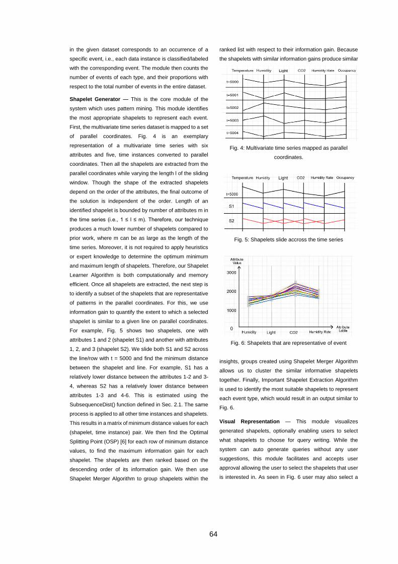
64

in the given dataset corresponds to an occurrence of a

specific event, i.e., each data instance is classified/labeled

with the corresponding event. The module then counts the

number of events of each type, and their proportions with

respect to the total number of events in the entire dataset.

Shapelet Generator — This is the core module of the

system which uses pattern mining. This module identifies

the most appropriate shapelets to represent each event.

First, the multivariate time series dataset is mapped to a set

of parallel coordinates. Fig. 4 is an exemplary

representation of a multivariate time series with six

attributes and five, time instances converted to parallel

coordinates. Then all the shapelets are extracted from the

parallel coordinates while varying the length l of the sliding

window. Though the shape of the extracted shapelets

depend on the order of the attributes, the final outcome of

the solution is independent of the order. Length of an

identified shapelet is bounded by number of attributes m in

the time series (i.e., 1 ≤ l ≤ m). Therefore, our technique

produces a much lower number of shapelets compared to

prior work, where m can be as large as the length of the

time series. Moreover, it is not required to apply heuristics

or expert knowledge to determine the optimum minimum

and maximum length of shapelets. Therefore, our Shapelet

Learner Algorithm is both computationally and memory

efficient. Once all shapelets are extracted, the next step is

to identify a subset of the shapelets that are representative

of patterns in the parallel coordinates. For this, we use

information gain to quantify the extent to which a selected

shapelet is similar to a given line on parallel coordinates.

For example, Fig. 5 shows two shapelets, one with

attributes 1 and 2 (shapelet S1) and another with attributes

1, 2, and 3 (shapelet S2). We slide both S1 and S2 across

the line/row with t = 5000 and find the minimum distance

between the shapelet and line. For example, S1 has a

relatively lower distance between the attributes 1-2 and 3-

4, whereas S2 has a relatively lower distance between

attributes 1-3 and 4-6. This is estimated using the

SubsequenceDist() function defined in Sec. 2.1. The same

process is applied to all other time instances and shapelets.

This results in a matrix of minimum distance values for each

(shapelet, time instance) pair. We then find the Optimal

Splitting Point (OSP) [6] for each row of minimum distance

values, to find the maximum information gain for each

shapelet. The shapelets are then ranked based on the

descending order of its information gain. We then use

Shapelet Merger Algorithm to group shapelets within the

ranked list with respect to their information gain. Because

the shapelets with similar information gains produce similar

Fig. 4: Multivariate time series mapped as parallel

coordinates.

Fig. 5: Shapelets slide accross the time series

Fig. 6: Shapelets that are representative of event

insights, groups created using Shapelet Merger Algorithm

allows us to cluster the similar informative shapelets

together. Finally, Important Shapelet Extraction Algorithm

is used to identify the most suitable shapelets to represent

each event type, which would result in an output similar to

Fig. 6.

Visual Representation — This module visualizes

generated shapelets, optionally enabling users to select

what shapelets to choose for query writing. While the

system can auto generate queries without any user

suggestions, this module facilitates and accepts user

approval allowing the user to select the shapelets that user

is interested in. As seen in Fig. 6 user may also select a

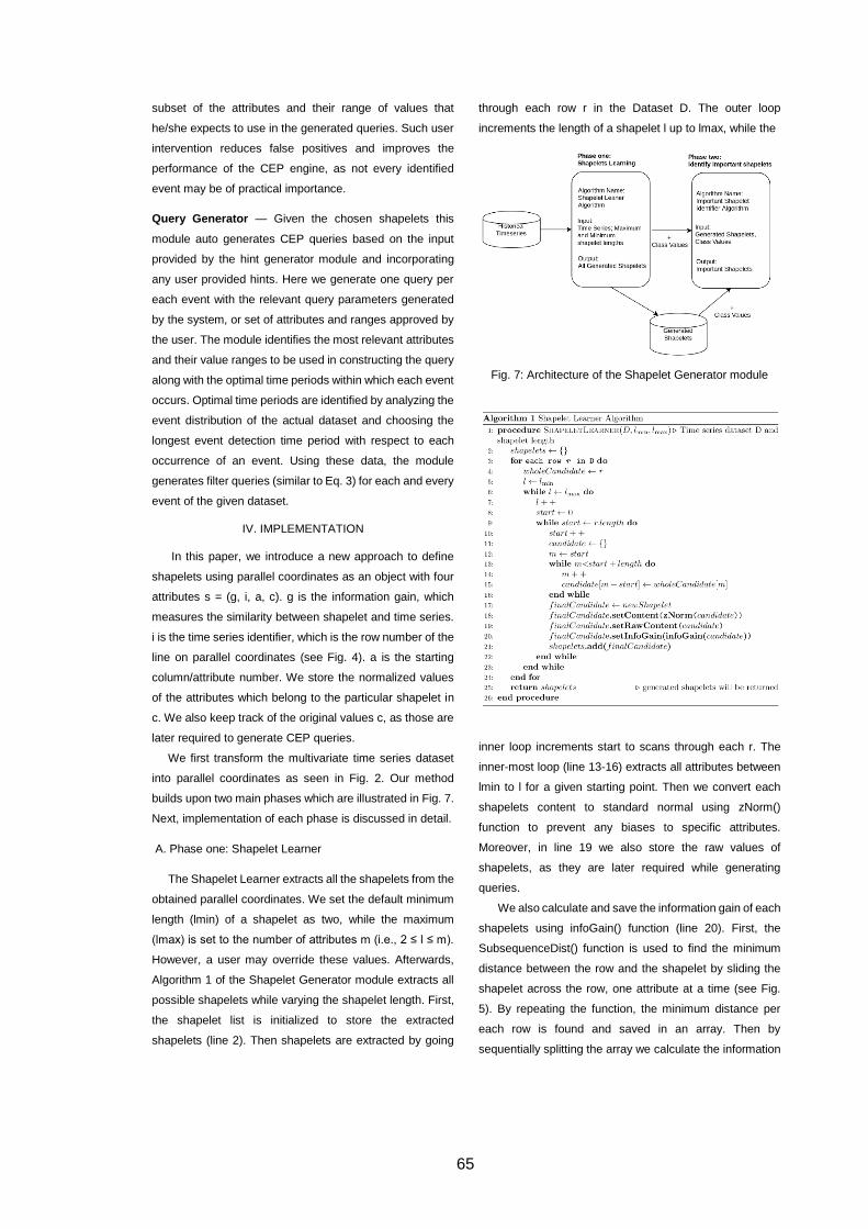
65

subset of the attributes and their range of values that

he/she expects to use in the generated queries. Such user

intervention reduces false positives and improves the

performance of the CEP engine, as not every identified

event may be of practical importance.

Query Generator — Given the chosen shapelets this

module auto generates CEP queries based on the input

provided by the hint generator module and incorporating

any user provided hints. Here we generate one query per

each event with the relevant query parameters generated

by the system, or set of attributes and ranges approved by

the user. The module identifies the most relevant attributes

and their value ranges to be used in constructing the query

along with the optimal time periods within which each event

occurs. Optimal time periods are identified by analyzing the

event distribution of the actual dataset and choosing the

longest event detection time period with respect to each

occurrence of an event. Using these data, the module

generates filter queries (similar to Eq. 3) for each and every

event of the given dataset.

IV. IMPLEMENTATION

In this paper, we introduce a new approach to define

shapelets using parallel coordinates as an object with four

attributes s = (g, i, a, c). g is the information gain, which

measures the similarity between shapelet and time series.

i is the time series identifier, which is the row number of the

line on parallel coordinates (see Fig. 4). a is the starting

column/attribute number. We store the normalized values

of the attributes which belong to the particular shapelet in

c. We also keep track of the original values c, as those are

later required to generate CEP queries.

We first transform the multivariate time series dataset

into parallel coordinates as seen in Fig. 2. Our method

builds upon two main phases which are illustrated in Fig. 7.

Next, implementation of each phase is discussed in detail.

A. Phase one: Shapelet Learner

The Shapelet Learner extracts all the shapelets from the

obtained parallel coordinates. We set the default minimum

length (lmin) of a shapelet as two, while the maximum

(lmax) is set to the number of attributes m (i.e., 2 ≤ l ≤ m).

However, a user may override these values. Afterwards,

Algorithm 1 of the Shapelet Generator module extracts all

possible shapelets while varying the shapelet length. First,

the shapelet list is initialized to store the extracted

shapelets (line 2). Then shapelets are extracted by going

through each row r in the Dataset D. The outer loop

increments the length of a shapelet l up to lmax, while the

Fig. 7: Architecture of the Shapelet Generator module

inner loop increments start to scans through each r. The

inner-most loop (line 13-16) extracts all attributes between

lmin to l for a given starting point. Then we convert each

shapelets content to standard normal using zNorm()

function to prevent any biases to specific attributes.

Moreover, in line 19 we also store the raw values of

shapelets, as they are later required while generating

queries.

We also calculate and save the information gain of each

shapelets using infoGain() function (line 20). First, the

SubsequenceDist() function is used to find the minimum

distance between the row and the shapelet by sliding the

shapelet across the row, one attribute at a time (see Fig.

5). By repeating the function, the minimum distance per

each row is found and saved in an array. Then by

sequentially splitting the array we calculate the information

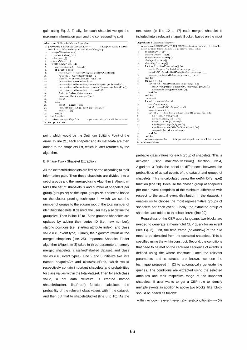
66

gain using Eq. 2. Finally, for each shapelet we get the

maximum information gain and the corresponding split

point, which would be the Optimum Splitting Point of the

array. In line 21, each shapelet and its metadata are then

added to the shapelets list, which is later returned by the

algorithm.

B. Phase Two - Shapelet Extraction

All the extracted shapelets are first sorted according to their

information gain. Then these shapelets are divided into a

set of groups and then merged using Algorithm 2. Algorithm

takes the set of shapelets S and number of shapelets per

group (groupsize) as the input. groupsize is selected based

on the cluster pruning technique in which we set the

number of groups to the square root of the total number of

identified shapelets. If desired, the user may also define the

groupsize. Then in line 12 to 15 the grouped shapelets are

updated by adding their series ID (i.e., raw number),

starting positions (i.e., starting attribute index), and class

value (i.e., event type). Finally, the algorithm return all the

merged shapelets (line 25). Important Shapelet Finder

algorithm (Algorithm 3) takes in three parameters, namely

merged shapelets, classified/labelled dataset. and class

values (i.e., event types). Line 2 and 3 initialize two lists

named shapeletArr and classValueProb, which would

respectively contain important shapelets and probabilities

for class values within the total dataset. Then for each class

value, a set data structure is created named

shapeletBucket. findProb() function calculates the

probability of the relevant class values within the dataset,

and then put that to shapeletBucket (line 8 to 10). As the

next step, (in line 12 to 17) each merged shapelet is

included into a relevant shapeletBucket, based on the most

probable class values for each group of shapelets. This is

achieved using maxProbClassVal() function. Next,

Algorithm 3 finds the absolute differences between the

probabilities of actual events of the dataset and groups of

shapelets. This is calculated using the getMinDifShape()

function (line 28). Because the chosen group of shapelets

per each event comprises of the minimum difference with

respect to the actual event distribution in the dataset, it

enables us to choose the most representative groups of

shapelets per each event. Finally, the extracted group of

shapelets are added to the shapeletArr (line 29).

Regardless of the CEP query language, two blocks are

needed to generate a meaningful CEP query for an event

(see Eq. 3). First, the time frame (or window) of the rule

need to be identified from the extracted shapelets. This is

specified using the within construct. Second, the conditions

that need to be met on the captured sequence of events is

defined using the where construct. Once the relevant

parameters and constructs are known, we use the

technique proposed in [2] to automatically generate the

queries. The conditions are extracted using the selected

attributes and their respective range of the important

shapelets. If user wants to get a CEP rule to identify

multiple events, in addition to above two blocks, filter block

should be added as follows:

within[window]{relevent−events}where[conditions]------ (4)

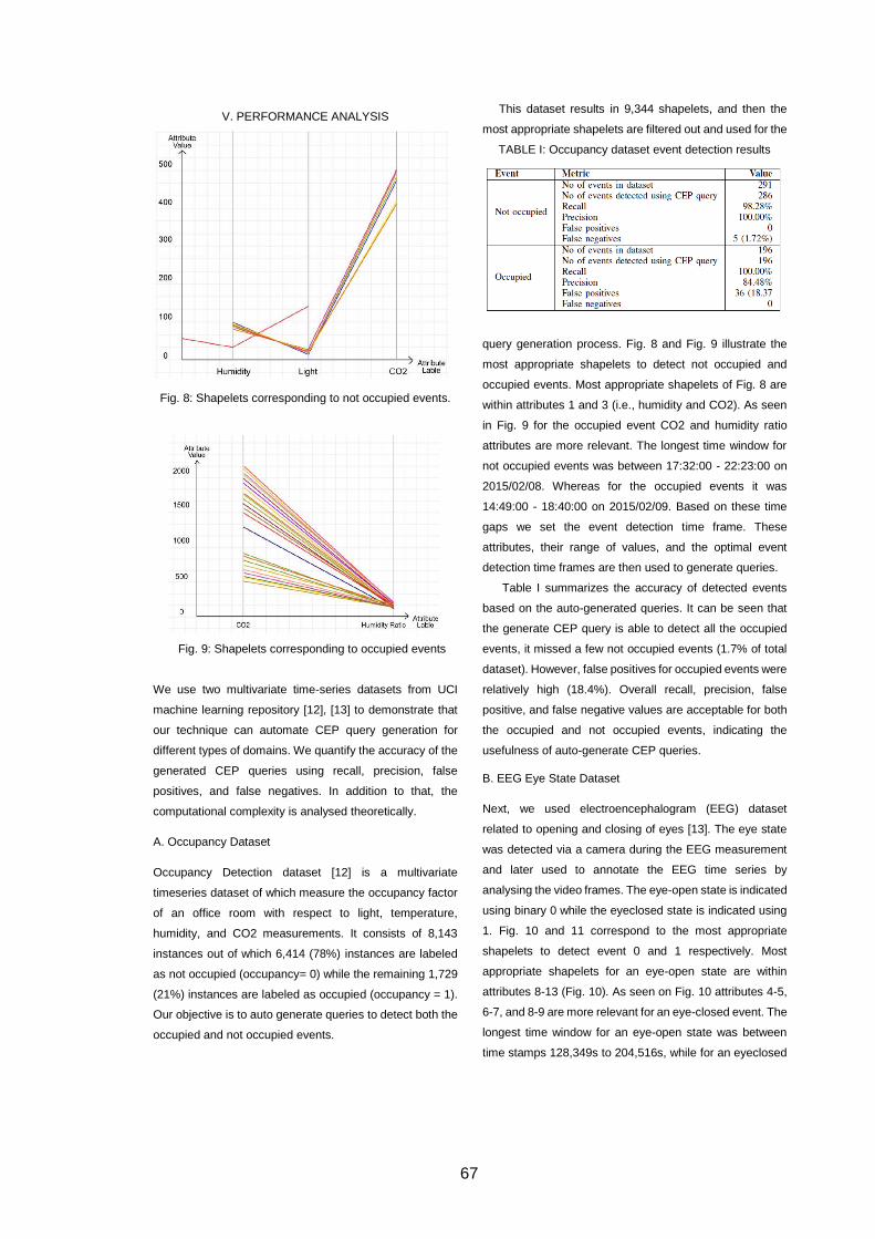
67

V. PERFORMANCE ANALYSIS

Fig. 8: Shapelets corresponding to not occupied events.

Fig. 9: Shapelets corresponding to occupied events

We use two multivariate time-series datasets from UCI

machine learning repository [12], [13] to demonstrate that

our technique can automate CEP query generation for

different types of domains. We quantify the accuracy of the

generated CEP queries using recall, precision, false

positives, and false negatives. In addition to that, the

computational complexity is analysed theoretically.

A. Occupancy Dataset

Occupancy Detection dataset [12] is a multivariate

timeseries dataset of which measure the occupancy factor

of an office room with respect to light, temperature,

humidity, and CO2 measurements. It consists of 8,143

instances out of which 6,414 (78%) instances are labeled

as not occupied (occupancy= 0) while the remaining 1,729

(21%) instances are labeled as occupied (occupancy = 1).

Our objective is to auto generate queries to detect both the

occupied and not occupied events.

This dataset results in 9,344 shapelets, and then the

most appropriate shapelets are filtered out and used for the

TABLE I: Occupancy dataset event detection results

query generation process. Fig. 8 and Fig. 9 illustrate the

most appropriate shapelets to detect not occupied and

occupied events. Most appropriate shapelets of Fig. 8 are

within attributes 1 and 3 (i.e., humidity and CO2). As seen

in Fig. 9 for the occupied event CO2 and humidity ratio

attributes are more relevant. The longest time window for

not occupied events was between 17:32:00 - 22:23:00 on

2015/02/08. Whereas for the occupied events it was

14:49:00 - 18:40:00 on 2015/02/09. Based on these time

gaps we set the event detection time frame. These

attributes, their range of values, and the optimal event

detection time frames are then used to generate queries.

Table I summarizes the accuracy of detected events

based on the auto-generated queries. It can be seen that

the generate CEP query is able to detect all the occupied

events, it missed a few not occupied events (1.7% of total

dataset). However, false positives for occupied events were

relatively high (18.4%). Overall recall, precision, false

positive, and false negative values are acceptable for both

the occupied and not occupied events, indicating the

usefulness of auto-generate CEP queries.

B. EEG Eye State Dataset

Next, we used electroencephalogram (EEG) dataset

related to opening and closing of eyes [13]. The eye state

was detected via a camera during the EEG measurement

and later used to annotate the EEG time series by

analysing the video frames. The eye-open state is indicated

using binary 0 while the eyeclosed state is indicated using

1. Fig. 10 and 11 correspond to the most appropriate

shapelets to detect event 0 and 1 respectively. Most

appropriate shapelets for an eye-open state are within

attributes 8-13 (Fig. 10). As seen on Fig. 10 attributes 4-5,

6-7, and 8-9 are more relevant for an eye-closed event. The

longest time window for an eye-open state was between

time stamps 128,349s to 204,516s, while for an eyeclosed

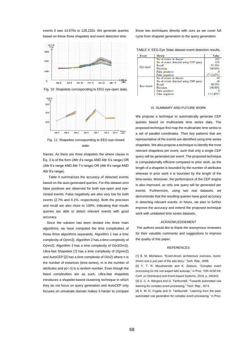
68

events it was 14,976s to 128,232s. We generate queries

based on these three shapelets and event detection time

Fig. 10: Shapelets corrosponding to EEG eye-open state.

Fig. 11: Shapelets corrosponding to EEG eye-closed

state.

frames. As there are three shapelets the where clause in

Eq. 3 is of the form (Attr 4’s range AND Attr 5’s range) OR

(Attr 6’s range AND Attr 7’s range) OR (Attr 8’s range AND

Attr 9’s range).

Table II summarizes the accuracy of detected events

based on the auto-generated queries. For this dataset zero

false positives are observed for both eye-open and eye-

closed events. False negatively are also very low for both

events (2.7% and 0.1%, respectively). Both the precision

and recall are also close to 100%, indicating that results

queries are able to detect relevant events with good

accuracy.

Since the solution has been divided into three main

algorithms, we have computed the time complexities of

those three algorithms separately. Algorithm 1 has a time

complexity of O(nm3). Algorithm 2 has a time complexity of

O(nm2). Algorithm 3 has a time complexity of O(n3/2m3).

Ultra-fast Shapelets [7] has a time complexity of O(pnm2)

and AutoCEP [2] has a time complexity of O(n2) where n is

the number of instances (time-series), m is the number of

attributes and p(< n) is a random number. Even though the

listed complexities are as such, Ultra-fast shapelets

introduces a shapelet-based clustering technique in which

they do not focus on query generation and AutoCEP only

focuses on univariate domain makes it harder to compare

those two techniques directly with ours as we cover full

cycle from shapelet generation to the query generation.

TABLE II: EEG Eye State dataset event detection results.

VI. SUMMARY AND FUTURE WORK

We propose a technique to automatically generate CEP

queries based on multivariate time series data. The

proposed technique first map the multivariate time series to

a set of parallel coordinates. Then key patterns that are

representative of the events are identified using time series

shapelets. We also propose a technique to identify the most

relevant shapeless per event, such that only a single CEP

query will be generated per event. The proposed technique

is computationally efficient compared to prior work, as the

length of a shapelet is bounded by the number of attributes

whereas in prior work it is bounded by the length of the

time-series. Moreover, the performance of the CEP engine

is also improved, as only one query will be generated per

events. Furthermore, using two real datasets, we

demonstrate that the resulting queries have good accuracy

in detecting relevant events. In future, we plan to further

improve the accuracy and extend the proposed technique

work with unlabeled time series datasets.

ACKNOWLEDGEMENT

The authors would like to thank the anonymous reviewers

for their valuable comments and suggestions to improve

the quality of this paper.

REFERENCES

[1] B. M. Michelson, “Event-driven architecture overview. event-

driven soa is just part of the eda story,” Tech. Rep., 2006.

[2] Y. T. R. Mousheimish and K. Zeitouni, “Complex event

processing for the non-expert with autocep,” in Proc. 10th ACM Intl.

Conf. on Distributed and Event-based Systems, 2016, p. 340343.

[3] G. C. A. Margara and G. Tamburrelli, “Towards automated rule

learning for complex event processing,” Tech. Rep., 2013.

[4] A. M. G. Cugola and G. Tamburrelli, “Learning from the past:

automated rule generation for complex event processing,” in Proc.

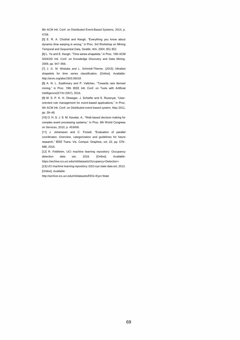
69

8th ACM Intl. Conf. on Distributed Event-Based Systems, 2014, p.

4758.

[5] E. R. A. Chotirat and Keogh, “Everything you know about

dynamic time warping is wrong,” in Proc. 3rd Workshop on Mining

Temporal and Sequential Data, Seattle, WA, 2004. 851 852

[6] L. Ye and E. Keogh, “Time series shapelets,” in Proc. 15th ACM

SIGKDD Intl. Conf. on Knowledge Discovery and Data Mining,

2009, pp. 947–956.

[7] J. G. M. Wistuba and L. Schmidt-Thieme. (2015) Ultrafast

shapelets for time series classification. [Online]. Available:

http://arxiv.org/abs/1503.05018

[8] A. N. L. Szathmary and P. Valtchev, “Towards rare itemset

mining,” in Proc. 19th IEEE Intl. Conf. on Tools with Artificial

Intelligence(ICTAI 2007), 2016.

[9] M. S. P. K. H. Obweger, J. Schiefer and S. Rozsnyai, “User-

oriented rule management for event-based applications,” in Proc.

5th ACM Intl. Conf. on Distributed event-based system, May 2011,

pp. 39–48.

[10] O. H. S. J. S. M. Kavelar, A., “Web-based decision making for

complex event processing systems,” in Proc. 6th World Congress

on Services, 2010, p. 453458.

[11] J. Johansson and C. Forsell, “Evaluation of parallel

coordinates: Overview, categorization and guidelines for future

research,” IEEE Trans. Vis. Comput. Graphics, vol. 22, pp. 579–

588, 2016.

[12] R. Feldheim, UCI machine learning repository: Occupancy

detection data set, 2016. [Online]. Available:

https://archive.ics.uci.edu/ml/datasets/Occupancy+Detection+

[13] UCI machine learning repository: EEG eye state data set, 2013.

[Online]. Available:

http://archive.ics.uci.edu/ml/datasets/EEG+Eye+State