Embed Size (px)
Citation preview

Abstract of thesis entitled
Passivity Assessment and Model Order Reduction for Linear
Time-Invariant Descriptor Systems in VLSI Circuit
Simulation
Submitted by
Zheng ZHANG
for the degree of Master of Philosophy
at the University of Hong Kong
in June 2010
This thesis presents some theoretical and numerical results for linear time-invariant
(LTI) descriptor systems (DSs), with emphasis on their corresponding passivity as-
sessment and model order reduction (MOR). DSs are widely used in VLSI circuit
modeling, including on-chip parasitics, RF passives, chip packagings, as well as lin-
earized models of transistor networks.
In the first part (Chapters 2 to 4), we focus on the passivity assessments of LTI
DSs. In Chapter 2, a generalized Hamiltonian method (GHM) and its half-size version
(HGHM) are developed. The most significant advantage of GHM/HGHM passivity
test is that they are purely algebraic routines, thereby rendering the test results
highly accurate. Not only can they tell a LTI DS is passive or not, but they also
accurately locate the possible nonpassive regions, thereby providing a versatile tool for
subsequent DS passivity enforcements. Chapter 3 presents a projector-based passivity
test for large-size LTI DS models which can not be readily tackled by GHM. It is the
first time that spectral projectors are used, which are based on our proposed fast
canonical projector construction, to efficiently decompose a large DS model into its
proper and improper subsystems. After the fast system decomposition, the proper

part is tested by GHM, via a fast iterative numerical implementation. Chapter 4
presents the S-parameter generalized Hamiltonian method (S-GHM), and also its
half-size algorithm (S-HGHM). Similar to GHM/HGHM, S-GHM and S-HGHM can
locate all possible nonpassive regions with high numerical accuracy. A passivity test
flow for admittance/impedance DSs is also proposed, based on S-GHM and S-HGHM
after a Moebious transform of DS state-space equations.
The second part (Chapters 5 & 6) solves two issues in DS MOR: passivity and im-
proper part preservation, as well as efficient MOR for multi-port DS models. Chapter
5 focuses on the first issue. The improper part of a DS is preserved by fast spectral
projector-based additive system decomposition. After that, the proper part is re-
duced via DS-format positive-real balanced truncation (DS-PRBT). Since the main
bottleneck of DS-PRBT is in solving the dual generalized algebraic Riccati equations
(GAREs), a generalized quadratic alternating direction implicit (GQADI) algorithm
is developed to efficiently compute the positive-real Gramians. To further speed
up the matrix solver, a low-rank version of GQADI (LR-GQADI) is also devised,
which reduces the complexity from O(n3) to O(n2). Chapter 6 constructs “good”
macromodels for multi-port LTI DSs, motivated by power grid simulation in mod-
ern VLSI design. Due to the large number of ports, existing MOR techniques are
not efficient for power grids. To overcome this problem, we develop a MOR routine
based on input matrix splitting, called BDSM (block-diagonal structured model or-
der reduction). The BDSM ROM (reduced-order model) is as accurate as standard
moment-matching MORs; its resultant ROMs are block-diagonal structured which
permits high efficiency for subsequent simulations; the BDSM ROM size can be fur-
ther scaled down for clock-gated power grid models; finally and most importantly,
unlike many existing power grid MORs that need to generate different ROMs for
different input waveforms, the resultant ROM from BDSM is reusable under various
input wave patterns.

Abstract word count: 504

Passivity Assessment and Model Order Reduction
for Linear Time-Invariant Descriptor Systems in
VLSI Circuit Simulation
by
Zheng ZHANG
B.Eng in 2008, Department of Electronic Science and Technology
Huazhong University of Science and Technology, P. R. China
A thesis submitted in partial fulfilment of the requirements for
the Degree of Master of Philosophy
at The University of Hong Kong.
June 2010

Declaration
I declare that this thesis represents my own work, except where due acknowledgement
is made, and that it has not been previously included in a thesis, dissertation or report
submitted to this University or to any other institution for a degree, diploma or other
qualifications.
Signed
Zheng ZHANG
i

Acknowledgements
This thesis could not have been finished without my supervisor Dr. Ngai Wong’s
guidance and supervision. In the past two years, Dr. Wong helped gear up my math-
ematics, pushed me forward to exercise independent thinking, and more importantly,
taught me to be self-motivated and enjoy research.
I would like to thank Prof. Cheng-Kuan Cheng, my supervisor for four months
during my visit to UCSD. In Prof. Cheng’s group, I learnt much about circuit the-
ory and power grid simulation. This pleasant experience has largely broadened my
research insights. Prof. Cheng’s patience, kindness, and continuous encouragement
not only impressed me, but also moved me.
Many thanks to my labmates at the University of Hong Kong. Thanks to CHEN
Quan, LEI Chi-Un and LIN Yu, WANG Yuanzhe, XU Yuanzhe and WANG Xiang,
for their valuable suggestions, kindly help, inspiring discussions, as well as lots of
laughters. I wish them best of luck in the future postgraduate or faculty careers. My
thanks also go to my friends in UCSD, especially HU Xiang, who helped me a lot in
the research of power grid simulation.
I am grateful to my family. Thanks to my parents and my sister for their care
since my childhood. And especially, I owe my thanks and love to my fiancee, who has
provided me with endless love, understanding and support in the past five years.
ii

Contents
Declaration i
Acknowledgements ii
Table of Contents iii
List of Tables ix
List of Figures xi
List of Abbreviations xv
1 Introduction 1
1.1 Research Motivation . . . . . . . . . . . . . . . . . . . . . . . . . . . 1
1.2 LTI State-Space Model . . . . . . . . . . . . . . . . . . . . . . . . . . 4
1.2.1 Standard State-Space Model . . . . . . . . . . . . . . . . . . . 4
1.2.2 Descriptor System . . . . . . . . . . . . . . . . . . . . . . . . 5
1.3 System Passivity and Existing Assessment Methods . . . . . . . . . . 7
1.3.1 Positive Realness and Bounded Realness . . . . . . . . . . . . 7
1.3.2 Methods for Standard State-Space Models . . . . . . . . . . . 8
1.3.3 Methods for Descriptor Systems . . . . . . . . . . . . . . . . . 9
1.4 Existing Model Order Reduction Schemes . . . . . . . . . . . . . . . 11
iii

1.4.1 Moment-Matching-Based MOR . . . . . . . . . . . . . . . . . 13
1.4.2 Gramian-Based MOR . . . . . . . . . . . . . . . . . . . . . . . 14
1.4.3 Passivity-Preserving DS MOR . . . . . . . . . . . . . . . . . . 17
1.5 Thesis Contributions . . . . . . . . . . . . . . . . . . . . . . . . . . . 19
1.5.1 Generalized Hamiltonian Methods (GHMs) . . . . . . . . . . . 19
1.5.2 Spectral Projector Technique and Fast GHM . . . . . . . . . . 20
1.5.3 S-Parameter GHMs (S-GHMs) . . . . . . . . . . . . . . . . . 20
1.5.4 Fast DS PRBT . . . . . . . . . . . . . . . . . . . . . . . . . . 21
1.5.5 Block-Diaognal Structured MOR for Multi-Port DSs . . . . . 21
2 Generalized Hamiltonian Methods (GHMs) 23
2.1 Introduction . . . . . . . . . . . . . . . . . . . . . . . . . . . . . . . . 23
2.2 Review of DS Positive Realness . . . . . . . . . . . . . . . . . . . . . 25
2.3 GHM and HGHM Theories for DSs . . . . . . . . . . . . . . . . . . . 27
2.3.1 GHM for General DSs . . . . . . . . . . . . . . . . . . . . . . 27
2.3.2 HGHM for Symmetric DSs . . . . . . . . . . . . . . . . . . . . 29
2.4 Admittance/Impedance DS Passivity Assessment . . . . . . . . . . . 30
2.4.1 Testing the Improper Part by ImPT . . . . . . . . . . . . . . 31
2.4.2 Testing the Proper Part by GHM and HGHM . . . . . . . . . 32
2.4.3 Equivalent Model Conversion . . . . . . . . . . . . . . . . . . 33
2.4.4 Connection to Traditional Hamiltonian Methods . . . . . . . . 35
2.4.5 Strict Positive Realness of Impulse-free DSs . . . . . . . . . . 36
2.5 Numerical Examples . . . . . . . . . . . . . . . . . . . . . . . . . . . 37
2.5.1 MNA Example for ImPT . . . . . . . . . . . . . . . . . . . . . 37
2.5.2 PEEC Example for GHM . . . . . . . . . . . . . . . . . . . . 39
2.5.3 A SAW Filter for HGHM . . . . . . . . . . . . . . . . . . . . . 40
2.5.4 CPU Time Comparison . . . . . . . . . . . . . . . . . . . . . . 40
iv

2.6 Summary . . . . . . . . . . . . . . . . . . . . . . . . . . . . . . . . . 41
3 Projector-Based Passivity Test for Large Descriptor Systems 43
3.1 Introduction . . . . . . . . . . . . . . . . . . . . . . . . . . . . . . . . 43
3.2 DS Passivity and System Decomposition . . . . . . . . . . . . . . . . 45
3.3 Matrix Projector Chain . . . . . . . . . . . . . . . . . . . . . . . . . . 46
3.3.1 Constructing Canonical projectors . . . . . . . . . . . . . . . . 49
3.3.2 Constructing Spectral Projectors . . . . . . . . . . . . . . . . 49
3.4 Passivity Test . . . . . . . . . . . . . . . . . . . . . . . . . . . . . . . 50
3.4.1 Additive Decomposition by Spectral Projectors . . . . . . . . 50
3.4.2 Reconstruction into a DS . . . . . . . . . . . . . . . . . . . . . 52
3.5 Implementation and Complexity . . . . . . . . . . . . . . . . . . . . . 53
3.5.1 Fast Spectral Projector Construction . . . . . . . . . . . . . . 53
3.5.2 Fast GHM Test for Proper-Part Passivity . . . . . . . . . . . . 56
3.5.3 Complexity Analysis . . . . . . . . . . . . . . . . . . . . . . . 59
3.6 Numerical Examples . . . . . . . . . . . . . . . . . . . . . . . . . . . 62
3.6.1 Projector-Based Decomposition . . . . . . . . . . . . . . . . . 62
3.6.2 Proper Part Testing . . . . . . . . . . . . . . . . . . . . . . . 64
3.7 Discussions . . . . . . . . . . . . . . . . . . . . . . . . . . . . . . . . 67
3.8 Summary . . . . . . . . . . . . . . . . . . . . . . . . . . . . . . . . . 68
3.9 Appendices . . . . . . . . . . . . . . . . . . . . . . . . . . . . . . . . 69
3.9.1 Matrix Chain with Canonical Projectors . . . . . . . . . . . . 69
3.9.2 Spectral Projectors from Canonical Projectors . . . . . . . . . 72
3.9.3 Outline of the LUQ Factorization . . . . . . . . . . . . . . . . 73
4 S-Parameter Generalized Hamiltonian Methods (S-GHMs) 76
4.1 Introduction . . . . . . . . . . . . . . . . . . . . . . . . . . . . . . . . 76
4.2 Review of Passivity Check for S-Parameter Models . . . . . . . . . . 78
v

4.3 S-GHM and S-HGHM . . . . . . . . . . . . . . . . . . . . . . . . . . 80
4.3.1 S-Parameter GHM (S-GHM) Theory . . . . . . . . . . . . . . 80
4.3.2 S-Parameter HGHM (S-HGHM) for Symmetric DSs . . . . . . 82
4.4 Passivity Test of DSs . . . . . . . . . . . . . . . . . . . . . . . . . . . 84
4.4.1 Passivity Test of S-Parameter DSs . . . . . . . . . . . . . . . . 84
4.4.2 Passivity Test of Hybrid DSs . . . . . . . . . . . . . . . . . . . 86
4.4.3 Comparison with Traditional Approaches . . . . . . . . . . . . 87
4.4.4 Numerical Issues . . . . . . . . . . . . . . . . . . . . . . . . . 88
4.5 Numerical Examples . . . . . . . . . . . . . . . . . . . . . . . . . . . 89
4.5.1 A Synthetic DS Model . . . . . . . . . . . . . . . . . . . . . . 89
4.5.2 A Symmetric S-Parameter Three-Terminal Filter . . . . . . . 92
4.5.3 A Symmetric Admittance PEEC Reduced Model . . . . . . . 93
4.5.4 A Multi-Port DS Model . . . . . . . . . . . . . . . . . . . . . 95
4.6 Discussions . . . . . . . . . . . . . . . . . . . . . . . . . . . . . . . . 96
4.7 Summary . . . . . . . . . . . . . . . . . . . . . . . . . . . . . . . . . 97
4.8 Appendix . . . . . . . . . . . . . . . . . . . . . . . . . . . . . . . . . 98
5 Fast Positive-Real Balanced Truncation of Descriptor Systems 100
5.1 Motivation . . . . . . . . . . . . . . . . . . . . . . . . . . . . . . . . . 101
5.2 Preliminaries . . . . . . . . . . . . . . . . . . . . . . . . . . . . . . . 103
5.2.1 Problems in DS MOR . . . . . . . . . . . . . . . . . . . . . . 103
5.2.2 Projected GALEs and GAREs . . . . . . . . . . . . . . . . . . 104
5.3 DS-MOR via DS-PRBT . . . . . . . . . . . . . . . . . . . . . . . . . 107
5.3.1 Additive Decomposition . . . . . . . . . . . . . . . . . . . . . 107
5.3.2 PRBT of the Proper Subsystem . . . . . . . . . . . . . . . . . 108
5.4 GQADI and Low-Rank GQADI . . . . . . . . . . . . . . . . . . . . . 110
5.4.1 GQADI . . . . . . . . . . . . . . . . . . . . . . . . . . . . . . 110
vi
5.4.2 Well Posedness . . . . . . . . . . . . . . . . . . . . . . . . . . 111
5.4.3 Convergence . . . . . . . . . . . . . . . . . . . . . . . . . . . . 113
5.4.4 Low-Rank GQADI (LR-GQADI) . . . . . . . . . . . . . . . . 115
5.4.5 Numerical Complexity . . . . . . . . . . . . . . . . . . . . . . 116
5.5 Experimental Results . . . . . . . . . . . . . . . . . . . . . . . . . . . 117
5.5.1 Subsystem Extraction . . . . . . . . . . . . . . . . . . . . . . 117
5.5.2 Comparison of GARE Solvers . . . . . . . . . . . . . . . . . . 118
5.5.3 Model Reduction Results . . . . . . . . . . . . . . . . . . . . . 119
5.6 Summary . . . . . . . . . . . . . . . . . . . . . . . . . . . . . . . . . 121
5.7 Appendices . . . . . . . . . . . . . . . . . . . . . . . . . . . . . . . . 121
5.7.1 Derivation of GQADI . . . . . . . . . . . . . . . . . . . . . . . 121
5.7.2 Proof of Lemma 5.1 . . . . . . . . . . . . . . . . . . . . . . . . 123
6 Block-Diagonal Structured Model Reduction for Power Grid Anal-
ysis 125
6.1 Introduction . . . . . . . . . . . . . . . . . . . . . . . . . . . . . . . . 126
6.2 Review of Power Grid MOR . . . . . . . . . . . . . . . . . . . . . . . 128
6.2.1 Power Grid Model . . . . . . . . . . . . . . . . . . . . . . . . 128
6.2.2 Problems with Standard Krylov-Subspace Projection . . . . . 129
6.3 BDSM Scheme . . . . . . . . . . . . . . . . . . . . . . . . . . . . . . 131
6.3.1 Input Matrix Splitting . . . . . . . . . . . . . . . . . . . . . . 132
6.3.2 Block-Diagonal Structured Projection . . . . . . . . . . . . . . 133
6.3.3 Numerical Complexity . . . . . . . . . . . . . . . . . . . . . . 135
6.4 Fast Power Grid Simulation . . . . . . . . . . . . . . . . . . . . . . . 137
6.4.1 BDSM-Based Simulation . . . . . . . . . . . . . . . . . . . . . 137
6.4.2 Problem Size Scaling . . . . . . . . . . . . . . . . . . . . . . . 139
6.4.3 Parallel Computation . . . . . . . . . . . . . . . . . . . . . . . 141
vii

6.5 Discussions of BDSM . . . . . . . . . . . . . . . . . . . . . . . . . . . 141
6.5.1 Comparison with Existing Power Grid MORs . . . . . . . . . 141
6.5.2 A Variant: Row-by-Row BDSM Scheme . . . . . . . . . . . . 143
6.5.3 System Passivity . . . . . . . . . . . . . . . . . . . . . . . . . 144
6.6 Numerical Results . . . . . . . . . . . . . . . . . . . . . . . . . . . . . 146
6.6.1 MOR Efficiency and Accuracy . . . . . . . . . . . . . . . . . . 146
6.6.2 Time-Domain Performance . . . . . . . . . . . . . . . . . . . . 149
6.7 Summary . . . . . . . . . . . . . . . . . . . . . . . . . . . . . . . . . 151
7 Thesis Conclusion 152
7.1 Part 1: DS Passivity Assessments . . . . . . . . . . . . . . . . . . . . 152
7.2 Part 2: DS Model-Order Reduction . . . . . . . . . . . . . . . . . . . 154
Bibliography 156
Publications during M.Phil Study 171
viii

List of Tables
2.1 GHM test results for the reduced model. . . . . . . . . . . . . . . . . 40
2.2 GHM and HGHM test results for the SAW model. . . . . . . . . . . . 41
2.3 CPU times (sec) of different DS passivity tests. . . . . . . . . . . . . 42
3.1 Total CPU times in DS index check . . . . . . . . . . . . . . . . . . . 62
3.2 CPU times excluding proper-part passivity check . . . . . . . . . . . 63
3.3 CPU times of full-size GHM and fast GHM tests on the proper subsystem. 67
4.1 Applicability of different passivity tests . . . . . . . . . . . . . . . . . 87
4.2 S-GHM/S-HGHM test results for the order-4 DS. . . . . . . . . . . . 91
4.3 Experimental results of various passivity tests for the three-terminal
filter model. . . . . . . . . . . . . . . . . . . . . . . . . . . . . . . . . 93
4.4 S-GHM and S-HGHM test results for the admittance reduced model
(on the Moebius-transformed system). . . . . . . . . . . . . . . . . . 94
4.5 CPU time (sec) comparison of S-GHM and S-HGHM. . . . . . . . . . 95
5.1 CPU times (sec) of DS decompositions. . . . . . . . . . . . . . . . . . 117
5.2 CPU times (sec) of solving one GARE (5.13a) . . . . . . . . . . . . . 117
6.1 Comparison of various multi-port MOR schemes. In SVDMOR, α
represents the port compression ratio. . . . . . . . . . . . . . . . . . . 142
ix

6.2 CPU times (sec) of various MOR schemes. In SVDMOR, we match the
moments of the approximated low-rank transfer matrix after terminal
reduction. In EKS, the moments of the response under unit impulse
excitations are captured, but the transfer matrix’s moments can not
be captured, therefore, the EKS ROM is not reusable. . . . . . . . . . 148
6.3 CPU times (sec) of 1000-point backward Euler time-domain simulation
via ROMs obtained by multi-point projection. . . . . . . . . . . . . . 149
x

List of Figures
2.1 An illustrative example for nonpassive region identification. . . . . . . 34
2.2 The complete passivity test flow for DSs, including regular systems. . 35
2.3 ImPT test for the MNA model [the iteration number means i in (2.20)]. 38
2.4 GHM and frequency sweeping results for the PEEC model. . . . . . . 39
2.5 Real part of Hr(s). . . . . . . . . . . . . . . . . . . . . . . . . . . . . 40
2.6 HGHM test for the SAW model. . . . . . . . . . . . . . . . . . . . . . 41
3.1 Flowchart for the proposed DS passivity test in a pseudocodes style. . 53
3.2 (a) Bode plots of the original, proper- and improper-subsystem re-
sponses. (b) Error between the original system and the sum of decom-
posed subsystems. . . . . . . . . . . . . . . . . . . . . . . . . . . . . . 64
3.3 Eigenspectrum of the generalized Hamiltonian matrix pencil (J ,K)for the PEEC model. Only the results close to the imaginary axis are
plotted. . . . . . . . . . . . . . . . . . . . . . . . . . . . . . . . . . . 65
3.4 Eigenspectrum of the generalized Hamiltonian matrix pencil (J ,K) forthe order-980 RLC model. Only the results close to the imaginary axis
are plotted. . . . . . . . . . . . . . . . . . . . . . . . . . . . . . . . . 65
xi

3.5 Passivity test results for the order-10913 DS model. (a) Eigenspectrum
of the generalized Hamiltonian matrix pencil (J ,K). Only the results
close to the imaginary axis are plotted. (b) Zoom-in of the eigenvalues
with small real parts (circled in the left plot). . . . . . . . . . . . . . 66
4.1 Illustrative examples for different kinds of DSs. (a) A globally strictly
passive DS. This DS has no crossover points and its transfer matrix is
always unit-bounded. (b) A consistently nonpassive DS. This DS does
not have any crossover points, but it is nonpassive at any frequency
point. (c) A DS with locally passive and nonpassive regions. This DS
is nonpassive in intervals l2 = (ω1, ω2), l4 = (ω3, ω4) and l6 = (ω5, ω6). 84
4.2 S-GHM and S-HGHM test results for the order-4 DS model. . . . . . 91
4.3 S-GHM and S-HGHM test results for the three-terminal filter. . . . . 92
4.4 S-GHM and S-HGHM test results on the Moebius-transformed transfer
function of the order-53 admittance reduced model. . . . . . . . . . . 94
4.5 The real part of the transfer function of the original order-53 admit-
tance DS model. The dots are the results from S-GHM and S-HGHM
tests, which are accurately located at the boundaries of passivity vio-
lations. . . . . . . . . . . . . . . . . . . . . . . . . . . . . . . . . . . . 95
4.6 S-GHM/S-HGHM test results for the multi-port S-parameter DS model.
The dots are the results from S-GHM and S-HGHM tests, which are
accurately located at the boundaries of passivity violations. . . . . . . 96
5.1 (a) A C-V loop. (b) An L-I cutset. . . . . . . . . . . . . . . . . . . . 103
5.2 (a) An index-1 circuit without any L-V cutsets or C-V loops. (b) An
index-2 circuit with a C-V loop formed by Vin and C1. . . . . . . . . 104
xii

xiii
5.3 Approximate Hankel singular values of the proper subsystem of ckt3.
Hankel singular values refer to the singular values of LTE0R (i.e., σ1,
σ2, · · · in Step 3 of Algorithm 5.3). . . . . . . . . . . . . . . . . . . . 118
5.4 (a) Frequency response (port-1) of ckt3 and the reduced models (or-
der=50) obtained by PRIMA and DS-PRBTs (solving the GAREs by
LR-GQADI and Newton’s iteration, respectively). (b) Relative errors. 119
5.5 GHM passivity test results show that the reduced model is passive.
(a) The eigenvalues of the generalized Hamiltonian matrix pencil. (b)
Zoom in of the central part. . . . . . . . . . . . . . . . . . . . . . . . 120
6.1 The BDSM model reduction scheme for a linear network with m input
ports, which is based on column-by-column moment matching. After
input matrix splitting, the original model is decomposed into m MIMO
subsystems. Then using the projection process, Hir(s) captures the
first l moments of H(s)’s i-th column. Finally, the parallel connection
of all ROMs guarantees the preservation of H(s)’s first l moments. . . 136
6.2 Projection matrix construction in the proposed BDSM scheme. Here,
Mj = ((s0C −G)−1C)j−1
(s0C−G)−1B, j = 1, · · · , l. The i-th columns
ofMj ’s are grouped to form Vi (i = 1, · · · ,m). And then Vi is computed
such that Vi = Vi, for i = 1, · · · , m. Note that in PRIMA the
projection matrix for (6.1) is constructed without clustering, such that
V = spanM1, · · · ,Ml with more computational cost. . . . . . . . . 138
6.3 The upper part represents a power grid with consideration of clock
gating; the bottom part is the RLC model. . . . . . . . . . . . . . . . 145
6.4 The matrix structures of ckt1’s ROMs, obtained from BDSM and
PRIMA, respectively. . . . . . . . . . . . . . . . . . . . . . . . . . . . 147
6.5 Comparison of MOR accuracy for ckt1. . . . . . . . . . . . . . . . . . 148

xiv
6.6 The voltage waveforms of node-37 in ckt3. . . . . . . . . . . . . . . . 150

List of Abbreviations
LTI linear time-invariant
DS descriptor system
MOR model order reduction
ROM reduced-order model
EROM effective reduced-order model
IC integrated circuit
EDA electronic design automation
CAD computer aided design
VLSI very large-scale integration
MEMs micro-electromechanical systems
EM electromagnetic
PEEC partial element equivalent circuit
VF vector fitting
pMOR parameterized model order reduction
vMOR variational model order reduction
PRIMA passive and reduced-order interconnect macromodeling algorithm
MNA modified nodal analysis
RLC resistor, inductor and capacitor
PVL Pade via Lanczos
MPVL matrix Pade via Lanczos
xv
xvi
EKS extended Krylov subspace
POD propoer orthogonal decomposition
BDSM block-diagonal structured model order reduction
BT balanced truncation
PRBT positive-real balanced truncation
BRBT bounded-real balanced truncation
DS-BT balanced truncation for descriptor systems
DS-PRBT positive-real balanced truncation for descriptor systems
ETBR extended truncated balanced realization
PSD positive semidefinite
ImPT improper part test
GHM generalized Hamiltonian method
HGHM half-size generalized Hamiltonian method
S-GHM S-parameter generalized Hamiltonian method
S-HGHM S-parameter half-size generalized Hamiltonian method
LMI linear matrix inequality
SHH skew-Hamiltonian/Hamiltonian
ARE algebraic Riccati equation
GARE generalized algebraic Riccati equation
GALE generalized algebraic Lyapunov equation
ADI alternating direction implicit
LR-ADI low-rank alternating direction implicit
QADI quadratic alternating direction implicit
LR-QADI low-rank quadratic alternating direction implicit
GQADI generalized quadratic alternating direction implicit
LR-GQADI low-rank generalized quadratic alternating direction implicit
SVD singular value decomposition

Chapter 1
Introduction
1.1 Research Motivation
Macromodeling is a very important step in the computer-aided design (CAD) of
very large-scale integration (VLSI). Typical examples include (but are not restricted
to): modeling of on-chip parasitic effects (such as interconnects and power ground
networks), chip packaging, microelectronic-mechanical systems (MEMS), analog and
radio-frequency (RF) circuits and components (such as on-chip inductors), chemical
or biological systems. Normally, these systems, components or structures are de-
scribed by detailed mathematical models such as differential equations. Based on
these models, simulation, analysis, verification and optimization procedures can be
performed before the final manufacturing step.
This thesis focuses on one of the important modeling frameworks: linear time-
invariant descriptor system (LTI DS) [1–3], which is a generalization of the standard
state-space model [4] and has found increasing applications in VLSI CAD. Typical
DS applications include: description of linear circuits [5] [such as those containing
only resistors (R), capacitors (C) and/or inductors (L)], discretized electromagnetic
(EM) equations [6] used in accurate parasitic extractions, linearization of nonlinear
1

2
systems [7] (such as analog and RF circuits, MEMS devices etc.). Recently, DS tech-
nique has also been used in data fittings [49, 50] that attempt to build behavioral
models of electronic components/systems from some available response data. These
frequency-domain or time-domain data may be from practical measurements or sim-
ulation results generated by complex mathematical models.
Specifically, this thesis addresses two issues about LTI DS: model order reduction
(MOR) and passivity characterization.
MOR is a popular and indispensable step to reduce circuit simulation complexity
in VLSI design flow. In practical VLSI design, the linear circuits (such as those
from parasitic extraction) and nonlinear blocks (e.g., those functional or logic blocks
containing transistors, diodes or MEMS devices) can be extremely complex, rendering
direct computer-aided simulation impractical or prohibitively time-consuming. A
viable solution is to approximate the original models, which are constantly of high
orders and thus difficult to solve, by reduced-order models (ROMs) that are amenable
for efficient computer simulation.
System passivity [8–14] is required in the physical modeling and MOR procedures
of linear passive systems (such as RLC models of interconnects and power grids, EM
extraction of on-chip inductors, data fitting of electrical packagings). This is because:
from the physical perspective, all RLC networks are energy-consuming or equiva-
lently dissipative systems, and thereby can not generate energy internally. However,
the system passivity may be lost during the process of MOR, which results in unsound
physical behaviors. Specifically, from the control perspective, all passive sub-blocks
connected together would yield a globally stable system; while stable but nonpassive
models may lead to unstable global behaviors (such as blowing-up node voltage). A
remedy for nonpassive models is passivity enforcement [10,11]. Passivity enforcement
consists of two steps. First, the models are checked by passivity verification algo-
rithms [8–14], to see if they are globally passive. Second, if nonpassive, the models

3
are slightly perturbed (subject to some accuracy criteria), such that the new models
are passive in the whole frequency band. From the numerical perspective, passivity
verification is the main bottleneck, due to its expensive computational load, as well
as high accuracy requirements.
Therefore, this thesis is devoted to passivity and MOR of LTI DSs. In the system
passivity part, we try to solve the following problems:
1. Flexible passivity assessment algorithms for reduced DS models with impedance
or admittance parameters.
2. Fast algorithms of passivity assessment to large-scale DSs, such as those from
EM solvers.
3. Passivity verification technique for DSs with scattering port parameters. This
case is mostly encountered in high-speed circuit modeling and EM component
description.
In the DS MOR part, we address two issues:
1. Passivity-preserving MOR for DSs based on fast numerical implementation. In
the MOR flow, we also aim to preserve the possible improper part of a DS,
subject to some numerical accuracy requirements.
2. Efficient MOR for multi-port (or many-port) DSs. This issue is mainly encoun-
tered in the simulation of power grid networks [91], whose large port number
makes traditional MOR approaches inefficient. We aim to develop more effi-
cient power grid MOR, such that the subsequent simulation can be significantly
speeded up.
Before unfolding the contributions of this thesis in later chapters, we begin with
some preliminaries about state-space modeling technique, and briefly review some
existing results regarding passivity assessments and DS MORs.

4
1.2 LTI State-Space Model
A LTI system is one that satisfies the following two conditions:
• Linearity, which means that the input-output relationship is a linear map.
Specifically, if the input uk(t) generates an output yk(t), then the scaled and
summed input∑
ckuk(t) would generate a scaled and summed output∑
ckyk(t).
• Time invariance, which means that whether we apply an input to a system
at time t or after a delay td, the output will be identical except for a time
delay of td. For example, if y(t) is the output excited by u(t), then the output
corresponding to u(t− td) is y(t− td).
1.2.1 Standard State-Space Model
A LTI standard state-space model is described by
dx(t)
dt= Ax(t) +Bu(t), y = Cx(t) +Du(t), (1.1)
where x ∈ Rn denotes the state variables, A ∈ R
n×n, B ∈ Rn×m, C ∈ R
p×n and
D ∈ Rp×m are system matrices. The input matrix B maps the input vector u(t) to
the state variables x(t), while the output matrix C maps x(t) to the output response
y(t).
Assume the above system is zero initial-conditioned. In Laplace domain, (1.1) can
be written as
sX(s) = AX(s) +BU(s), Y (s) = CX(s) +DU(s), (1.2)
where X(s), U(s) and Y (s) are the Laplace transforms of x(t), u(t) and y(t), respec-
tively. The frequency-domain input-output relationship can be characterized through

5
the transfer matrix H(s)
Y (s) = H(s)U(s), where H(s) = C(sI − A)−1B︸ ︷︷ ︸Hsp(s)
+D ∈ Cp×m.
(1.3)
The transfer matrix H(s) is a proper matrix function that approaches D as s→∞,
while its strictly proper part is denoted by Hsp(s) which is zero at s =∞. Note that
H(s) can also be written as a rational matrix function:
H(s) =R1
s− p1+ · · ·+ Rn
s− pn︸ ︷︷ ︸Hsp(s)
+D ∈ Cp×m
(1.4)
where pk (k = 1, · · · , n) are the eigenvalues of A, Rk ∈ Rp×m is the corresponding
residual matrix. The system is strictly stable if spec(A) = p1, · · · , pn ⊂ C−, where
C− denotes the open left-hand side of the complex plane. This is because, in this
case, the impulse response would not have exponentially increasing terms, which is
readily seen by inverse Laplace transform.
1.2.2 Descriptor System
In practical circuit modeling, a descriptor system (DS), rather than a standard state-
space model, is more frequently used. A DS is also called as generalized system or
singular system, which is a superset of standard state-space models. We study a
linear time-invariant (LTI) DS in the form
E dxdt
= Ax+Bu, y = Cx+Du, (1.5)
where E,A ∈ Rn×n, B ∈ R
n×m, C ∈ Rp×n and D ∈ R
p×m. Also, u ∈ Rm, y ∈ R
p and
x ∈ Rn are the input, output and state vectors, respectively. The matrix E is generally

6
singular with rank(E) ≤ n. We assume that the matrix pencil λE−A is regular, i.e.,
det(λ0E−A) 6= 0 for some λ0 ∈ C. Then, there always exist nonsingular W,T ∈ Rn×n
that transform E and A into the so-called Weierstrass canonical form [15]:
E = W
Iq 0
0 N
T, A = W
J 0
0 In−q
T, (1.6)
where Iq denotes an identity matrix of order q (though the dimension is omitted
whenever it is clear from context). The matrix J corresponds to the finite eigenvalues
of λE−A, whereas N is nilpotent and corresponds to the infinite eigenvalues. When
all eigenvalues of J have negative real parts, the pencil λE − A is said to be stable.
The nilpotency index µ of N , viz. Nµ−1 6= 0 and Nµ = 0, is called the index of the
matrix pencil λE − A.
Referring to the Weierstrass canonical form (1.6), we define the left and right
(spectral) projectors, Pl and Pr, respectively, as [16, 19, 20]
Pl = W
Iq 0
0 0
W−1, Pr = T−1
Iq 0
0 0
T. (1.7)
Obviously, Pl and Pr are the projectors onto the left and right deflating subspaces,
respectively, corresponding to the finite eigenvalues along the left and right deflating
subspaces corresponding to the eigenvalue at infinity, whereas Ql = I − Pl and Qr =
I − Pr are the complementary projectors.
Using (1.6) and partitioning [Cp C∞ ] = CT−1 and [BTp BT
∞]T = W−1B con-
formal to (1.6), the DS transfer function H(s) = D + C(sE − A)−1B of (1.5) can be

7
expressed as
H(s) = D + C(sE −A)−1B = D +[Cp C∞
] (sIq − J)−1
−(In−q − sN)−1
Bp
B∞
=D − C∞B∞ +
Hsp(s)︷ ︸︸ ︷Cp(sIq − J)−1Bp︸ ︷︷ ︸
Hp(s)
−sC∞NB∞ − s2C∞N2B∞ − s3C∞N3B∞ − · · ·︸ ︷︷ ︸H∞(s)
, (1.8)
where Hp(s) is the proper part of H(s) (bounded as s → ∞), Hsp(s) is the strictly
proper part that approaches zero as s→∞ andH∞(s) the improper part (unbounded
as s→∞).
1.3 System Passivity and Existing Assessment Meth-
ods
In this section, we introduce the concepts related to system passivity, and briefly re-
view existing passivity assessment techniques. A system is passive if it cannot generate
energy internally; it is strictly passive (or dissipative) if it consumes energy [21]. The
passivity of a LTI system is normally described by the positive realness or bounded
realness of its transfer function.
1.3.1 Positive Realness and Bounded Realness
Assume that H(s) is the transfer matrix of a LTI system, and it is a square matrix
(which means the system’s input and output port numbers are identical). Depending
on the physical meaning of H(s), system passivity can be defined in different ways.
In passivity assessments and circuit model reduction, we are interested in the case
that H(s) represents admittance/impedance parameters or scattering parameters.
If the square matrix function H(s) represents the frequency-domain admittance

8
or impedance of an electrical network, the corresponding LTI system is (strictly)
passive if and only if H(s) is (strictly) positive real. A square transfer matrix H(s)
is (strictly) positive real if and only if [21, 39]:
1. H(s) has no poles in Re(s) > 0;
2. H(s) = H(s) for all s ∈ C;
3. H(s) +H∗(s) ≥ 0 (> for strict positive realness) for all Re(s) ≥ 0.
The first condition means that the system is stable; the second condition implies that
the system matrices are real; and the third condition implies that all eigenvalues of
H(s) +H∗(s) are positive real for any s = jω where ω ∈ R is the angular frequency.
If H(s) represents the frequency-domain scattering matrix (normally used in EM
modeling or high-frequency applications such as RF circuit design), the system is
(strictly) passive if and only if H(s) is (strictly) bounded real [13, 21]:
1. H(s) is analytic on the open right half plane (Re(s) > 0);
2. H(s) = H(s) for all s ∈ C;
3. I −H∗(s)H(s) ≥ 0 for all Re(s) ≥ 0.
Also, condition 1 requires the system to be stable. Condition 2 implies that all
singular values of H(s) should be unit bounded (i.e., ≤ 1, where < corresponds to
the strict bounded realness), for any s = jω.
1.3.2 Methods for Standard State-Space Models
We consider the LTI standard state-space model (1.1), whose transfer matrix is readily
given as H(s) = C(sI−A)−1B+D. It is obvious that D should be a positive definite
matrix if this LTI is strictly passive. Numerous passivity verification approaches have
been developed for LTI standard state-space models, mainly including:

9
1. Frequency sweeping method [8,9]. The idea is to check the positive (or bounded)
realness of H(s) at a set of sampling points s = jωk (k = 1, 2, · · · ), along
the imaginary axis. The idea is simple, but the algorithms are not reliable:
although an adaptive sampling and a reciprocal sampling methods are developed
in [8] and [9] respectively, some nonpassive regions among neighboring sampling
points are missed and passivity can not be accurately tested by finite sampling.
2. Linear matrix inequality (LMI) and algebraic Riccati equation (ARE) [4, 21],
which were developed in control community. The LMI method tests system
passivity via convex programming at the cost of O(n6) complexity. Using Schur
complement [40], the LMI test can be converted to the ARE test and then
solved at the cost of O(n3). The ARE test checks system passivity via solving
the positive-real (or bounded-real) Gramian matrices [4] of an LTI system. Un-
fortunately, neither of them could tell the system’s possible non-passive regions,
which is necessary in the subsequent passivity enforcements.
3. Hamiltonian method [10–12]. This is the most accurate and widely used algo-
rithm in passivity assessments and enforcements. By solving the eigenvalues
of a size-2n Hamiltonian matrix, every possible nonpassive region can be accu-
rately located. Recently, the half-size variants [13, 14] of Hamiltonian methods
have been developed, with better numerical accuracy and an 8× speedup over
traditional Hamiltonian methods.
1.3.3 Methods for Descriptor Systems
The passivity assessment of a DS is much more involved. The difficulty arises from
the singularity of E in the system model, which may lead to an improper part in the
transfer matrix. For example, for an admittance/impedance case, according to the
definition of system passivity, H(s) is (strictly) positive real if and only if [39]:

10
1. The only admissible form of the improper part is H∞(s) = sM1, and M1 must
be either zero (which means the DS being impulse-free) or positive semidefinite
(i.e., M1 ≥ 0).
2. The proper part Hp(s) is (strictly) positive real.
These dual conditions imply that we need to test both the improper and proper parts
of a DS. However, the two parts can not be easily separated. Although the Weierstrass
canonical form can be used, it is extremely expensive (with O(n4) complexity) and
numerically unstable, thus only applicable to theoretical analysis. Compared with its
standard state-space counterpart, DS passivity test is much less investigated. Existing
DS passivity characterization methods include:
1. Half-unit circle sweeping [41]. This method first maps the s-domain to z-domain
to obtain a nonsingular system. Then the sampling points are selected along the
half-unit circle on the complex plane, followed by checking the positive realness
or bounded realness at these sampling points. Similar to the sweeping methods
used for standard state-space models, this approach may miss nonpassive regions
between the neighboring sampling points and is therefore inaccurate.
2. Passivity test by LMI or generalized algebraic Riccati equation (GARE) [39,
42–45]. For admittance/impedance DSs [39, 42–44], these methods require the
DSs to be admissible, impulse-free or minimally realized, which are normally
not satisfied in practice. Note that for S-parameter DSs, the model is not re-
quired to be impulse-free in passivity test, since the DS should be nonpassive
if an improper part is involved in its transfer matrix. Similar to their counter-
parts for standard state-space models, LMI and GARE based methods generally
can not tell the nonpassive regions, and therefore can not be used in passivity
enforcement flows.

11
3. Decompose-and-test methods [20, 46, 47]. These methods first decompose the
original DS to an improper part and a proper subsystem via Weierstrass de-
composition [46, 47] or spectral projector technique [20]. After decomposition,
the proper part can be converted to a standard state-space model, and then
checked by existing approaches (e.g., Hamiltonian methods). Therefore, these
methods can detect and locate the possible nonpassive regions. The drawbacks
of these methods include: 1) the Weirstrass decomposition is prohibitively ex-
pensive and unstable; 2) the spectral projector technique, which is obtained via
canonical projector [20], requires expensive matrix factorization (e.g., full-size
SVD), thus is infeasible for medium and large-size DSs; 3) converting the proper
subsystem to a standard state-space model is in general numerically expensive,
unstable and error-prone.
1.4 Existing Model Order Reduction Schemes
Numerous MOR algorithms have been developed to generate macromodels for fast
circuit simulation. According to their application areas, these MOR algorithms can
be classified into three groups.
1. Linear MOR [22–30]. These techniques are mostly used to reduce the com-
plexity of parasitic networks (such as RLC networks of interconnects or power
grids, which are described by differential circuit equations or discretized EM
models), RF passive components that require accurate description by full-wave
EM equations, chip packagings. Linear MORs can be implemented by various
approaches, such as Krylov-subspace projection [22–25], Gramian-based reduc-
tion originated from control community [27–30], proper orthogonal decomposi-
tion (POD) reduction [61,62]. Given a set of measured or simulated data, linear
macromodels can also be constructed via data fittings [48–50].

12
2. Nonlinear MOR [31–33]. They are mainly used to simplify the mathematical
models of nonlinear devices (e.g., transistors, MEMS devices) or systems. Non-
linear systems are very common in circuit design, including almost all analog
and RF blocks, such as amplifiers, mixers, oscillators, phase-locked loops (PLL)
etc. For different situations (e.g., strongly nonlinear circuits, weakly nonlinear
circuits, or nonlinear circuits with periodic or quasi-periodic signals), the MOR
algorithms might be slightly different such that some important properties or
parameters could be captured (e.g., high-order harmonics, signal intermodula-
tion).
3. Parametric MOR (pMOR) [34, 35]. Parametric MOR is also referred to varia-
tional MOR [36] (vMOR), which is developed to address the variation-induced
issues in circuit and system modeling. Typical cases are geometric variations [34]
and process uncertainty [35] that are inherent in manufacturing, as well as tem-
perature fluctuations [37, 38] that have strong impacts on interconnect signal
delay, power consumption and chip reliability. pMOR can be applied to both
linear and nonlinear systems.
In this thesis, we focus on linear MORs with application to LTI DSs. In these
MOR schemes, the projection technique is the most widely used method. From the
black-box perspective, system models can also be constructed by data fitting methods,
either in standard state-space [48] or DS form [49,50]. However, these macromodeling
techniques are beyond our scope.
In projection-based linear MORs, we attempt to find two projection matrices W
and V (with W T , V ∈ Rn×q) for the DS (1.5), such that a much smaller size-q model
can be generated:
Erdz(t)
dt= Arz(t) +Bru(t), yr(t) = Crz(t) (1.9)

13
with Er = W TEV , Ar = W TAV , Br = W TB and Cr = CV , such that Hr(s) =
Cr(sEr − Ar)−1Br ≈ H(s) or Yr(s) = Hr(s)U(s) ≈ Y (s), subject to some ac-
curacy requirements. Typical methods of constructing the projection matrices in-
clude: POD [61, 62], moment-matching technique [22, 25, 52], and Gramian-based
method [26,29,30]. The reader is referred to the survey paper [51] and the references
therein for details. In circuit context, moment-matching and Gramian-based MORs
are most widely applied and thereby reviewed below.
1.4.1 Moment-Matching-Based MOR
Many moment-matching MOR algorithms stem from Pillage’s work on asymptotic
waveform evaluation (AWE) [52]. In the frequency domain, the transfer matrix H(s)
of the DS in (1.5) can be written as a Taylor expansion around s0
H(s) =∑
Mk(s− s0)k, for k = 0, 1, · · · . (1.10)
The matrix Mk(s0) = CF kR is the order-k moment at expansion point s0, with
R = (s0E − A)−1B and F = −(s0E − A)−1E. The idea of moment matching is
that we can approximate H(s) by capturing some of its important moment matrices.
In [52], the moments are computed in an explicit way, which suffers from numerical
instability.
An alternative is to match the moments implicitly by Krylov subspace method.
An order-l block Krylov subspace Kl (F,R) is defined as
Kl (F,R) = spanR,FR, · · · , F l−1R
. (1.11)
For simplicity we assume that m = p. The matrix Pade via Lanczos algorithm

14
(MPVL) [25] constructs the projection matrices by
V = Kl (F,R) , W = Kl
(F , R
), with F = F T , R = (s0E − A)−TCT . (1.12)
By MPVL, a size-q ROM (1.9), with q = ml, could be constructed to capture the
first 2l moments of H(s), i.e.,
Hr(s) =∑
Mr,k(s− so)k, with Mr,k = Cr
(−(s0Er − Ar)
−1Er
)k(s0Er − Ar)
−1Br.
and Mr,k = Mk, for k = 0, 1, · · · , 2l − 1.
(1.13)
Obviously, the error between Hr(s) and H(s) is O((s− s0)
2l).
Another way to construct the projection matrices by only one Krylov subspace,
resulting in W = V . This method is called congruence transform [53], by which the
first l moments can be matched for a general DS model. For a symmetric model, such
as a RC network with voltage sources as excitations and port currents as outputs,
congruence transform can capture 2l moments.
1.4.2 Gramian-Based MOR
The Gramian-based MOR [26, 28–30, 57, 58] originated from the control community.
Compared with moment-matching methods, Gramian-based MORs have two advan-
tages: stability (or passivity) preservation for even unstructured system, plus an
analytical error bound for quantifying numerical accuracy. Here we give the basic
flows of classic balanced truncation (BT), as well as positive-real or bounded-real
balanced truncation (PRBT or BRBT) which preserve system passivity.
Given a stable LTI state-space model (1.1) (i.e., spec(A) ∈ C−), the controllability

15
Gramian Qc and observability Gramian Qo are defined as
Qc =
∫ ∞
0
eAtBBT eAT tdt, Qo =
∫ ∞
0
eAT tCTCeAtdt (1.14)
which are the symmetric positive semi-definite solutions to the dual Lyapunov equa-
tions
AQc +QcAT +BBT = 0, ATQo +QoA+ CTC = 0. (1.15)
Due to the positive semi-definiteness of the Gramians, there exist two factors Lc
and Lo, such that Qc = LcLTc and Qc = LoL
To . We compute the singular value
decomposition of LTo Lc:
LTo Lc =
[U1 U2
] Σ1
Σ2
[V1 V2
]T, (1.16)
where Σ1 = diag(σ1, ..., σq), Σ2 =diag(σq+1, ..., σn) and σ1 ≥ ... ≥ σq ≥ σq+1 ≥ ... ≥ σn
are called the Hankel singular values. To this end, the left projection matrix W and
the right projection matrix V are constructed as
W = LoU1Σ− 1
2
1 , V = LcV1Σ− 1
2
1 . (1.17)
Finally, the ROM could be constructed as Ar = W TAV , Br = W TB, Cr = CV . One
advantage of balanced truncation is that an upper error bound is provided for the
resulting transfer matrix
‖H(s)−Hr(s)‖∞ ≤ 2n∑
k=q+1
σk. (1.18)
Compared with moment-matching methods, BT is capable of providing stable ROMs
and an analytical error bound, but it is much more expensive (O(n3) complexity).

16
An ADI iteration and its low-rank variant (LR-ADI) are proposed in [57,58] to solve
Lyapunov equations at the cost comparable to that of Krylov-subspace projection.
The details of ADI and LR-ADI algorithms are not presented here, and interested
readers may refer to [57, 58] for details.
Classic BT can generate stable macromodels, but the ROMs are not guaranteed
to be passive, which is normally expected in interconnect and RF passive component
modeling. To preserve system passivity, PRBT (for admittance/impedance systems)
or BRBT (for scattering systems) can be used. In PRBT, we need to solve the dual
Lur’e equations [26] or algebraic Riccati equations (AREs) [30], which are essentially
equivalent. The dual AREs are formulated as
AQc +QcAT +
(QcC
T −B)P−1(CQc − BT ) = 0
ATQo +QoA+(QoB − CT
)P−1(BTQo − C) = 0
(1.19)
where P = D + DT > 0 for strict positive real systems, Qc and Qo (which are
positive semidefinite) denote the positive-real controllability Gramian and positive-
real observability Gramian, respectively. After computing Qc and Qo, the projection
matrices W and V can be computed in the same way as in classic BT. PRBT is the
same with BRBT, except for that the bounded real controllability and observability
Gramians Qc and Qo are the solutions to (1.19) after replacing P with I − DDT .
An ARE equation could be solved via Newton iteration, and inside each iteration a
Lyapunov equation needs to be solved. Recently, a quadratic ADI (QADI) is proposed
in [30] to solve the ARE at the cost of approximately only that of one Lyapunov
equation.
For the DS in (1.5), stability-preserving balanced truncation has also been de-
veloped based on solving the dual generalized Lyapunov equations. The ADI and
LR-ADI algorithms have also been extended to efficiently solve the dual generalized

17
Lyapunov equations. Details about DS BT and related fast matrix solvers could be
found in [54–56].
1.4.3 Passivity-Preserving DS MOR
In practice, almost all LTI models encountered in circuit simulation are in the DS
form, including linear circuit equations formulated by modified nodal analysis (MNA),
RF passive component models extracted by EM field solvers, as well as many lin-
earized models from nonlinear equations. For DS cases, the passivity-preserving MOR
becomes much more involved.
There indeed exists a special case: positive semidefinite (PSD) structured DS,
where passivity-preserving MOR could be easily performed. For example, in the
MNA formulation of linear RLC circuits, if we are interested in the port admittance
or impedance parameters, the DS matrices are PSD structured:
E ≥ 0, A+ AT ≤ 0, C = BT . (1.20)
Subsequently, using congruence transform would generate a positive-real ROM, as
detailed in the famous PRIMA paper [22]. But there are many cases where their
system matrices are not PSD structured, thus system passivity cannot be preserved
by simply using Krylov-subspace based moment matching. Even for a PSD structured
DS, system passivity could not be preserved by congruence transform when its transfer
matrix represents the scattering parameters.
To preserve system passivity during the MOR of general DSs, we need to use
passivity-preserving DS BT [16–18]. Assuming the DS (1.5) is impulse-free, the DS-
PRBT algorithm is based on solving the dual generalized algebraic Riccati equations

18
(GAREs):
AQcET + EQcA
T +(EQcC
T −B)P−1(CQcE
T − BT ) = 0
ATQoE + ETQoA+(ETQoB − CT
)P−1(BTQoE − C) = 0
(1.21)
with D + DT > 0. Similar to the classic BT and PRBT, we can get the Cholesky
factor (or square-root factor) of the Gramian matrices, such that Qc = LcLTc and
Qo = LoLTo . Then we continue to compute the skinny SVD:
LTo ELc =
[U1 U2
] Σ1
Σ2
[V1 V2
]T, (1.22)
where Σ1 and Σ2 contain the descending Hankel singular values. Finally, the pro-
jection matrices could be constructed as in (1.17), and the reduced-order model is
obtained by
Er = W TEV, Ar = W TAV, Br = W TB, Cr = CV, Dr = D. (1.23)
In the above MOR, the dual GARE (1.21) may be solved by state-of-the-art ma-
trix solvers in [59, 60]. These GARE solvers use Newton iteration that converts the
quadratic matrix equations (generalized algebraic Riccati equations) to linear matrix
equations (generalized Lyapunov functions), and then solve each generalized Lya-
punov equation by (LR)-ADI. Consequently, the overall cost approximates that of
solving tens of generalized Lyapunov functions. Note that some DSs may not be
impulse-free, and the improper part may be extracted by spectral projectors. If the
circuit topology is given, the spectral projector could be constructed by a closed
form [17,18]. Nevertheless, the spectral projector construction is not trivial for most
DSs (such as DS models from EM solvers). A fast numerical implementation will be

19
presented in Chapter 5.
1.5 Thesis Contributions
The work included in this thesis consists of two parts. Chapters 2 to 4 propose a set
of new methods for DS passivity assessments, including both admittance/impedance
DSs and S-parameter DSs; Chapter 5 and Chapter 6 address some issues involved in
DS MOR: passivity preservation and the multi-port problem.
1.5.1 Generalized Hamiltonian Methods (GHMs)
In Chapter 2, we present the generalized Hamiltonian method (GHM) for DSs with
admittance or impedance transfer matrices.
First, a pre-processing step called improper part test (IMPT), is proposed to
characterize the improper part without system decomposition. If the improper part
is passive, GHM could be used to test the proper part.
Then, GHM is proposed. GHM is a generalization (and superset) of the widely
used Hamiltonian method. But different from traditional Hamiltonian methods,
GHM can be used to test the passivity of both standard state-space models and
DS models, without system decomposition. Similar to the Hamiltonian method, the
proposed GHM is capable of detecting and locating every possible nonpassive region,
thus it could be used as a reliable test in DS passivity enforcements.
Then, we further develop a half-size variant of GHM, called HGHM. HGHM can be
used to test the passivity of symmetric DSs. On top of all the advantages of GHM,
HGHM is more efficient (8× faster over GHM). From the numerical perspective,
HGHM is also more reliable.

20
1.5.2 Spectral Projector Technique and Fast GHM
Chapter 3 presents a DS passivity test for large-scale systems, such as those from
EM solvers. We aim to efficiently test the proper part of a DS model even when its
improper part is nonpassive.
First, we present the theories regarding canonical projectors, and then show how
to construct a right (or left) spectral projector via a canonical projector technique.
Based on the spectral projector technique, the proper and improper parts of a DS
model can be separated in an elegant way.
However, the conventional canonical projector-based spectral projector construc-
tion is inefficient. To solve this problem, we present a fast numerical implementation,
based on sparse LU-based fast null space construction, as well as low-rank matrix
multiplication. To this end, the spectral projector could be efficiently computed for
large-scale DSs.
After decomposing the original DS into its proper and improper subsystems, the
improper part can be tested easily. To efficiently test the proper subsystem, we use
the GHM approach presented in Chapter 2, based on fast numerical implementation.
In our implementation, the multi-shift Arnoldi iteration [78] is extended to compute
those generalized eigenvalues close to the imaginary axis. Since only a small part
of the eigenvalues are needed for passivity test, the GHM-based verification can be
applied to large systems with size up to 104.
1.5.3 S-Parameter GHMs (S-GHMs)
Chapter 4 addresses the passivity test of a scattering DS, based on the bounded
realness of its transfer matrix.
We first extend the GHM theory to a scattering DS, to characterize the singular
values of its transfer matrix; then, for symmetric S-parameter DSs, a half-size variant

21
of S-GHM, called S-HGHM, with better numerical accuracy and efficiency, is also
developed.
With the S-GHM and S-HGHM theories, we can test general DS models very
efficiently. We also present an interesting method for admittance/impedance DS
passivity test: using Moebious transform, the original admittance/impedance DS is
converted to a new S-parameter model, which is then tested by S-GHM/S-HGHM.
1.5.4 Fast DS PRBT
Chapter 5 is concerned with Gramian-based passivity-preserving MOR of DSs. We
aim to solve two problems in DS MOR: 1) preservation of the possible improper part,
if any; 2) preservation of system passivity. To achieve these objectives, we first use
a spectral projector to extract the proper and improper subsystems efficiently; after
that, we use PRBT to get a ROM of the proper subsystem.
For the reduction of the proper subsystem, we develop a fast algorithm to solve
the dual generalized algebraic Riccati equations (GAREs). Unlike existing state-of-
the-art GARE solver that uses Newton’s iteration, we propose a generalized AQDI
(GQADI) to solve the dual GAREs with much shorter CPU times. We then give the
theoretical proofs of the convergence and well posedness of the proposed algorithm.
Finally, noting the positive semidefiniteness of the Gramians, a low-rank algorithm
called LR-GQADI is proposed, which solves the GARE with further speedup.
1.5.5 Block-Diaognal Structured MOR for Multi-Port DSs
Chapter 6 addresses the issue in the MOR of multi-port LTI descriptor systems.
Multi-port systems are normally used in power grid simulation. Due to the huge port
size, Krylov-subspace projections cannot generate good macromodels that allow fast
subsequent simulation.

22
Our proposed block-diagonal structured model reduction (BDSM) can generate
sparse and structured ROMs that can be efficiently simulated. First, using input ma-
trix splitting and parallel connection of LTIs, a block-diagonal structured (but much
larger) DS model is constructed, which has the same transfer matrix of the original
one. Then we use Krylov subspace to generate the projection matrices. In the pro-
jection matrix construction, the columns corresponding to different ports are sorted
to different groups, which finally results in block-diagonal structured projection ma-
trices and ROMs. The BDSM has several advantages: 1) it is based on exact moment
matching, thus it is very accurate; 2) it has the same size as traditional Krylov-
subspace MORs, but the resulting ROMs are sparse and block-diagonal structured;
3) its special structure allows fast computation and very flexible parallel implementa-
tion; 4) in power grid simulation, the problem size of the BDSM ROM can be further
scaled down, if the power gating technique is considered.

Chapter 2
Generalized Hamiltonian Methods
(GHMs)
A generalized Hamiltonian method (GHM) and its half-size variant (HGHM) are pro-
posed to characterize the spectral behaviors of descriptor systems (DSs). With the
preprocess ImPT (Improper Part Test), GHM and HGHM can be applied to test the
passivity of immittance (impedance or admittance) DSs without system decompo-
sition, system index assumption or minimal realization requirement, which are the
major bottlenecks of existing algebraic DS passivity tests. The proposed method
allows exact detection of nonpassive frequency intervals which is not possible with
frequency sweeping techniques. Numerical results confirm the effectiveness of the
proposed method.
2.1 Introduction
This work is motivated by the demand of passive modeling of admittance or impedance
on-chip components and electrical circuits in VLSI simulations [11,22,25]. In this case,
23

24
system passivity can be interpreted as the positive realness of system transfer ma-
trix, which is of great importance for stable global simulations. However, nonpassive
models may be generated from some stability-preserving algorithms (e.g., vector fit-
ting (VF) [48] and balanced truncations (PVL) [57, 58]) or even some theoretically
passivity-preserving techniques (e.g., [22]) on finite-precision machines. As a remedy,
passivity enforcement techniques [11] can eliminate or mitigate passivity violations.
These enforcements need to locate the possible nonpasive regions via passivity test in
advance. For regular (or nonsingular) systems, numerous passivity assessments have
been proposed. Readers are referred to [11,14] and the references therein.
Nevertheless, DS passivity tests are much less developed compared with their reg-
ular system counterparts. The O(n6) computation renders the extended LMI (linear
matrix inequality) tests [39, 42] impractical for general DSs. Reference [42] presents
a cheaper method based on generalized Schur decomposition, but it poses strict re-
strictions on system observability and controllability. Some literatures assess positive
realness via generalized algebraic Riccati equations (GAREs) [43,44], but the admis-
sible requirement is also a very strong condition for practical physical models. Fur-
thermore, none of these methods can locate the possible nonpassive frequency regions,
which is normally required in testing the validity of circuit and component models.
Some decompose-and-test flows [46, 47] require the DSs to be minimal, and the sys-
tem decomposition and transformation may induce large numerical errors (caused by
possibly ill-conditioned matrix inversions). The eigenvalue-based DS passivity test
in [64] is only applicable to scalar function. Frequency sweeping methods [20, 41]
detect nonpassive regions at a set of frequency points, but they may miss nonpassive
frequency intervals. Therefore, it is desirable to develop a passivity assessment that
can identify the nonpassive regions of general DSs efficiently and accurately.
We propose, for the first time, a flexible passivity test flow for general DSs based
on generalized Hamiltonian methods. The main contribution of this chapter includes:

25
1) GHM and HGHM to characterize the eigenvalues of DS spectral functions; 2) A
complete DS passivity test based on ImPT, GHM and HGHM to test the improper
and proper parts easily without system decomposition; 3) The observation that the
GHM- and HGHM-based passivity tests are the supersets of traditional Hamiltonian
method and its half-size [14] counterpart, respectively, as well as the connection of
GHM with GAREs [43, 44]. Part of this work is presented in [65], which mainly
discusses GHM and ImPT.
2.2 Review of DS Positive Realness
We first recall the positive realness of LTI models. For an immittance linear time-
invariant (LTI) system, the (strict) passivity is equivalent to its square transfer matrix
H(s) being (strictly) positive real [39]:
1. H(s) has no poles in Re(s) > 0;
2. H(s) = H(s) where o stands for the conjugate of o;
3. The spectral function G(jω) = (H(jω) +H∗(jω)) /2 ≥ 0 for all ω ∈ R (> for
strict positive realness), where ∗ means the conjugate transpose operation.
For a regular state-space system H(s) = C(sI −A)−1B+D, its positive realness can
be tested by the Hamiltonian matrix [14]:
M =
A −R
P −AT
(2.1)
of which any purely imaginary eigenvalue defines a boundary frequency of passivity
violations. In (2.1), A = A − B(D + DT )−1C, R = B(D + DT )−1BT and P =
CT (D +DT )−1C.

26
In circuit modeling and reduction, we usually use the LTI DS:
Ex = Ax+Bu, y = Cx+Du, (2.2)
where x ∈ Rn denotes the state variables, E,A ∈ R
n×n, B,CT ∈ Rn×m, D ∈ R
m×m,
and rank(E) ≤ n (“=” corresponds to regular cases). The transfer matrix of (2.2) is
H(s) = C(sE − A)−1B +D. (2.3)
Here (A,E) is assumed to be regular, i.e., det(sE −A) is not identically zero. There
exists a Weierstrass form [39]:
(A,E) = W (
F 0
0 In−q
,
Iq 0
0 N
)T, (2.4)
where W and T are nonsingular, Iq denotes an identity matrix of dimension q, F
and N (an index-µ nilpotent matrix, i.e., Nµ = 0 and Nµ−1 6= 0) correspond to the
finite and infinite generalized eigenvalues of (A,E), respectively. The Weierstrass
form implies
H(s) = Cp(sIq − F )−1Bp +M0︸ ︷︷ ︸Hp(s)
+
µ−1∑
k=1
skMk
︸ ︷︷ ︸Himp(s)
, (2.5)
where[Cp C∞
]= CT−1 and
Bp
B∞
= W−1B, M0 = D − C∞B∞, Mk =
−C∞NkB∞ (k = 1, ..., µ − 1). Hp(s) and Himp(s) are the proper and improper
parts, respectively. The immittance DS in (2.5) is passive if and only if [39]: 1) Hp(s)
is passive; 2) M1 ≥ 0 and Mk = 0 for any k ≥ 2. An LMI test [at the cost of O(n6)]
is developed in [39] for the characterization of DS positive realness.

27
1. Sufficient Condition: If there exists a solution X to the following LMIs:
ATX +XTA XTB − C
BTX − CT −D −DT
≤ 0, ETX = XTE ≥ 0, (2.6)
then H(s) defined by (2.3) is positive real.
2. Necessary Condition: Assume that (E,A,B,C,D) is a minimal realization
of H(s) and D +DT ≥ M0 +MT0 , then the LMIs in (2.6) have a solution X if
H(s) is positive real.
Obviously, besides the extremely expensive computation, the minimal realization
requirement is also highly restrictive.
2.3 GHM and HGHM Theories for DSs
2.3.1 GHM for General DSs
Theorem 2.1: Assume that λ is not an eigenvalue of (D+DT )/2 for the stable DS
(E,A,B,C,D) (i.e., any finite s satisfying det(A− sE) = 0 is located on the left half
plane), then λ is an eigenvalue of G(jω) if and only if jω is a generalized eigenvalue
of the matrix pencil (J, K), defined as
(J,K) = (
A+BQ−1C BQ−1BT
−CTQ−1C −AT − CTQ−1BT
,
E 0
0 ET
), (2.7)
where Q = (2λI −D −DT ). Note that the matrix J is a Hamiltonian matrix.
Proof: Assume that λ is an eigenvalue of the spectral function defined as G(jω) =
(H(jω) +H∗(jω)) /2. Since the system matrices are real, we haveH∗(jω) = HT (−jω),

28
then there exists x 6= 0, such that
2G(jω)x =
[C BT
]Ω−1
ω
B
−CT
+D +DT
x = 2λx. (2.8)
Here we have used Ωω to denote
jωE − A
jωET + AT
for simplicity. We could
rewrite (2.8) in a compact matrix form as
Q−1[C BT
]z = x (2.9)
with z = Ω−1ω
B
−CT
x 6= 0. By pre-multiplying both sides of (2.9) by Ω−1
ω
B
−CT
,
we further get
Ω−1ω
B
−CT
Q−1
[C BT
]z = z (2.10)
which is essentially equivalent to
Jz = jωKz. (2.11)
To this end, we have shown that the imaginary scalar jω is a generalized eigenvalue
of matrix pencil (J,K) if λ is an eigenvalue of G(jω).
To prove the converse, we denote w := Q−1[C BT
]z [which should be a
nonzero vector, since z 6= 0 in (2.10)]. Pre-multiplying both sides of (2.10) by
Q−1[C BT
], we would reach
Q−1[C BT
]Ω−1
ω
B
−CT
w = w, (2.12)

29
which is equivalent to (2.8), implying λ is an eigenvalue of G(jω) if jω is a generalized
eigenvalue of (J,K).
2.3.2 HGHM for Symmetric DSs
Next, we consider a special case: symmetric DSs. For symmetric DSs, the matrix pen-
cil in GHM theory could be reduced to a half-size one, and the imaginary eigenvalue
computation would be replaced by positive real eigenvalue calculation.
Theorem 2.2: For symmetric DSs [i.e., H(s) = HT (s)], if λ is not an eigenvalue
of D, the matrix pencil (J,K) defined in (2.7) could be reduced to a half-size matrix
pencil
(Jh, Kh) = (A+B(λI −D)−1C, EA−1E), (2.13)
and accordingly, the generalized eigenvalue jω could be replaced by β = ω2.
Proof: Given a symmetric DS, we haveH∗(jω) = H(−jω) = −C(jωE +A)−1B+
D. In such case, the matrix pencil (J,K) could be written as
(J,K) =
S T
−T −S
,
E 0
0 E
(2.14)
where S = A + B(2λI − 2D)−1C, T = B(2λI − 2D)−1C. Noting that (J ′, K ′) =
Z(J,K)ZT has the same generalized eigenvalues as (J,K) if Z is invertible, if we set
Z =
I I
I −I
, then we could get a structured matrix pencil
(J ′, K ′) =
0 2(S − T )
2(S + T ) 0
,
2E
2E
. (2.15)

30
Assume that λ is an eigenvalue of G(jω), then jω is a generalized eigenvalue of (J,K)
(which is a trivial result from the proposed GHM theory). Because (J,K) and (J ′, K ′)
have the same spectrum, jω should also be a generalized eigenvalue of (J ′, K ′). Based
on this, we know that there exist x1 and x2, such that
−jωE S − T
S + T −jωE
x1
x2
= 0,
x1
x2
6= 0. (2.16)
This is a size-2n matrix equation, which can be further reduced to
(Jh − ω2Kh)x1 = 0, x1 6= 0. (2.17)
Therefore, β = ω2 is a generalized eigenvalue of (Jh, Kh).
Conversely, by setting x2 = jω(S − T )−1x1, we can arrive at (2.16) from (2.17)
and then go back to Theorem 2.1.
2.4 Admittance/Impedance DS Passivity Assess-
ment
DS passivity test is more involved than its standard state-space model because it
requires testing both the proper and improper part. In this section, we introduce
a passivity verification flow for DSs with admittance or impedance transfer matrix,
based on the proposed GHM and HGHM theory. In the first step, a preprocessing
step is needed to check the improper part.

31
2.4.1 Testing the Improper Part by ImPT
We begin the passivity verification with ImPT (Improper Part Test), which is de-
veloped to characterize the improper part of a DS. Denoting the highest order of
Himp(s) by the integer ζ − 1 (1 ≤ ζ ≤ µ), then the improper part could be written as
Himp(s) =ζ−1∑k=1
skMk with Mζ−1 6= 0. Given a set of positive real scalars si (i = 1, 2, ...)
with si+1 = ηsi (η > 1), the matrix norm of H(si) could be written as
‖H(si)‖ = sζ−1i
∥∥∥∥∥Mζ−1 +Mζ−2
si+ · · ·+ Hp(si)
sζ−1i
∥∥∥∥∥ . (2.18)
Clearly, if si is large enough, the highest-order term sζ−1i Mζ−1 would dominate H(si).
As a result, we have Mζ−1 +Mζ−2
si+ · · ·+ Hp(si)
sζ−1
i
≈Mζ−1, which further implies
‖H(si+1)‖‖H(si)‖
≈ ηζ−1. (2.19)
Consequently, the system index can be evaluated by
ζ =
[logη(
‖H(si+1)‖‖H(si)‖
)
]+ 1, (2.20)
where [o] represents rounding operation. We select positive real scalar si in the
computation based on two reasons: 1) for a stable DS, its poles are located on the
left-half plane, thus the peaks from the proper part could be avoided; 2) numerical
calculation on real numbers is faster and more reliable than on complex numbers.
In practical implementations, η can be set around 10 − 100, and we may start with
a randomly selected number (e.g., s1 = 105) and then replace si with si+1 until∣∣∣[logη(
‖H(si+1)‖‖H(si)‖
)]− logη(
‖H(si+1)‖‖H(si)‖
)∣∣∣ < δ. Here δ is a small positive constant used to
control numerical errors. Since si is exponentially increased, the iteration would
converge very fast. If ζ ≥ 3, we have M2 6= 0 and thus the DS is nonpassive, since

32
repeated infinite poles exist in the transfer matrix. If ζ = 2, we have H(si) =
Hp(si) + Himp(si) ≈ siM1 + M0, then the coefficient of the improper part could be
computed by
M1 ≈H(si+1)−H(si)
si+1 − si. (2.21)
With a numerical error control, (2.21) can be used to compute M1 with a high ac-
curacy. In impulse-free DSs, the denominator in (2.20) might approach zero in case
M0 = 0, and directly using (2.20) may give erroneous results. In this case, we replace
H(si) with H(si) + Im to compute ζ.
Hereafter, we assume that Himp(s) has been checked by ImPT, ζ ≤ 2, and M1 ≥ 0
(or else the passivity test terminates since we have already known the improper part
is nonpassive). In this case Hp(jω) + H∗p (jω) = H(jω) + H∗(jω), then the proper
part can be tested by GHM or HGHM.
2.4.2 Testing the Proper Part by GHM and HGHM
In admittance/impedance passivity assessment, we are most interested in the situ-
ations where the positive realness is violated. Clearly, λ = 0 is the boundary case
where a system becomes nonpassive from being passive (or vice versa). By setting
λ = 0, we could have (J,K) = (J0, K0) with
J0 = M =
A −R
P −A
, K0 = K. (2.22)
Here M is the Hamiltonian matrix [66] defined in (2.1). For HGHM, setting λ = 0
gives a half-size matrix pencil
(Jh0, Kh0) = (A−BD−1C, EA−1E). (2.23)

33
The resulting matrix pencils (J0, K0) and (Jh0, Kh0) could be used to test the positive
realness of a DS, i.e., the passivity of an admittance or impedance DS model: any
purely imaginary (or positive real) generalized eigenvalue jω (or β = ω2) of (J0, K0)
(or (Jh0, Kh0) for symmetric DSs) defines a crossover angular frequency ω where
the eigenvalue of G(jω) crosses the imaginary axis on the complex plane. These
crossover points can be used to locate the possible nonpassive frequency intervals.
Denote Θ := ω1, ..., ωp where ωi (i = 1, ..., p) represents the p crossover points
obtained from GHM or HGHM, then the passive and nonpassive regions of H(jω)
can be identified as follows.
1. If Θ is empty, test G(jω0) at a randomly selected sampling point ω0. The
system is strictly passive if G(jω0) > 0, otherwise nonpassive at any frequency point.
2. If Θ is not empty, test G(jω′k) at ω
′k ∈ `k (k = 1, 2, ..., p+1) where `1 =(0, ω1),
`i =(ωi−1, ωi) for i = 2, ..., p and `p+1 =(ωp,∞). If G(jω′k) > 0, then the DS is passive
in the interval `k, otherwise nonpassive in `k.
An illustrative example is shown in Fig. 2.1. For this DS, GHM and HGHM
produce 3 crossover points. We randomly select one sampling point in each interval.
Since G(jω′3) < 0 and G(jω′
k) > 0 for k = 1, 2, 4, the DS is nonpassive in (ω2, ω3) but
passive in other frequency bands.
2.4.3 Equivalent Model Conversion
At the first glance, GHM/HGHM test requires D + DT to be nonsingular, which is
not always satisfied in practical DSs. In this case, we need to perform an equivalent
model conversion in advance. Assume that α ∈ R is not an eigenvalue of D, then
Dα = αI −D is nonsingular. A new DS H ′(s) realized by (E ′, A′, B′, C ′, D′) can be

34
0 1 2 3 4 5 6 7−0.03
−0.02
−0.01
0
0.01
0.02
0.03
0.04
0.05
0.06
Angular frequency
G(jω
)
ω1
ω2
ω3ω’
1 ω’2 ω’
3ω’
4
Figure 2.1: An illustrative example for nonpassive region identification.
constructed as
E ′ =
E
0
, A′ =
A
D−1α
, B′ =
B
I
,
C ′ =[C I
], D′ = αI.
(2.24)
We note that the resulting DS model has the same transfer matrix as the original one
[i.e, H ′(s) = H(s)], but D′ +D′T and D′ are nonsingular. Therefore, the proper part
of H(s) can be assessed by testing the passivity of H ′(s) via GHM or HGHM. We
remark that, given a standard state-space model (with E = I), the equivalent model
conversion would generate a DS model, which can be tackled by GHM, or HGHM if
its transfer matrix is symmetric. The main computation in GHM and HGHM tests
is the O(n3) generalized eigenvalue solution. HGHM-based test should be 8 times
faster than GHM-based method due to its half-size nature. With equivalent model
conversion, GHM (HGHM) can also be applied to (symmetric) regular systems with
singular D+DT (D) where traditional Hamiltonian method and half-size singularity
test [14] fail to work.

35
Traditional Hamiltonian
methods
No
No
Given a DS H(s) described by (E,A,B,C,D)
Is E singular?
System is non-passive
Use equivalent model conversion in ( 2.24 )
Form (J 0 , K 0 ) in (2.22)
Any crossover points?
Compute M 1 by ( 2.21 )
Form M in (2.1)
Any crossover points?
System is passive
D+D singular?
D+D singular? M 1 >=0 ?
Compute at
Yes
Yes
Yes
Yes
No
Yes
No
No
Yes
Yes
No >0?
T
T
Compute by ( 2.20 )
=2
=1 >=3
ImPT
Is H(s) symmetric?
Form (J h0 , K h0 ) in (2.23)
Is H(s) symmetric?
Form M h in (2.25)
Yes No
No Yes
No
GHM/HGHM
>0 for all k? Yes
No
Figure 2.2: The complete passivity test flow for DSs, including regular systems.
2.4.4 Connection to Traditional Hamiltonian Methods
An interesting observation is that the proposed GHM and HGHM methods are in fact
a superset of the widely used Hamiltonian method [11] and its half-size variant [14].
Given a standard state-space models (E = I), the generalized eigenvalue solution
of (J,K) reduces to the eigenvalue solution of J defined in (2.7), which has been
widely used in passivity enforcements [11] for nonpassive regular state-space models.
To check system passivity, we could set λ = 0 and get J0 = M [defined in (2.1)].
For symmetric standard state-space models, the generalized eigenvalue solution of

36
(Jh0, Kh0) in (2.23) can be replaced by the eigenvalue solution of
Mh = A(A−BD−1C) (2.25)
which is the half-size singularity test recently proposed in [14].
Therefore, Hamiltonian method and its half-size variant are special cases of GHM
and HGHM, respectively. All of them detect passivity violation regions by finding
boundary frequencies, but GHM and HGHM can deal with DSs as well as regular
systems, without restrictions on D, which implies much wider applications. The
complete test flow is illustrated in Fig. 2.2, where ImPT and traditional Hamiltonian
methods are also included.
2.4.5 Strict Positive Realness of Impulse-free DSs
GARE [43,44] is widely used to characterize the positive realness of impulse-free DSs.
This part shows its connection with GHM.
Lemma 2.1: Suppose (A,E) is regular, impulse-free and D+DT > 0 (otherwise,
the proposed equivalent model conversion can be performed to meet this requirement),
then the following statements are equivalent.
1) H(s) is strictly positive real.
2) The generalized algebraic Riccati equation (GARE)
ATX +XT A+XT RX + P = 0, ETX = XTE ≥ 0 (2.26)
has a solution X such that (A+ RX,E) is stable.
3) The matrix pencil (J0, K0) has no purely imaginary generalized eigenvalues and
M0 > 0 [M0 is defined in (2.5)].
Proof: The equivalence of 1) and 2) has been proved in [43]. The proof of 3)⇒1)

37
is trivial based on the GHM theory. From Statement 2), we get
det(J0 − sK0) = det
I
−XT I
(J0 − sK0)
I
X I
= det
sE − (A+ RX) 0
0 sET + (AT +XT RT )
= det(sE − (A+ RX)
)det(sE + (A+ RX)
).
(2.27)
Since (A + RX,E) is stable, A + RX ± jωE is nonsingular. Therefore, the matrix
pencil (J0, K0) has no purely imaginary generalized eigenvalues. The equivalence of
1) and 2) also implies M0 > 0, therefore, 3) can be derived from 2) and the above
statements are equivalent.
We remark that GARE requires (E,A) to be admissible, but GHM only requires
M1 = MT1 . GHM can locate the passive/nonpassive regions whereas GARE cannot.
2.5 Numerical Examples
This section presents some numerical examples to verify the proposed passivity test
flow. All experiments are performed in MATLAB R2006a on a 2.66-GHz 2G-RAM
PC.
2.5.1 MNA Example for ImPT
This 9-port order-10913 MNA model describes a large RLC network. Since the RLC
circuit is passive, ζ should be 1 or 2 and M1 ≥ 0. To show the convergence of ImPT,
we set s1 = 103 and η = 10, and plot the numerical error εi for i = 1, 2, .., 6 in

38
10−4
10−2
100
102
104
−60
−50
−40
−30
−20
−10
0
10
Frequency (Hz)
Mag
nitu
de (
dB)
(b)
Original response, port(2,2)
10−4
10−2
100
102
104
−80
−70
−60
−50
−40
−30
−20
−10
Frequency (Hz)M
agni
tude
(dB
)
(c)
Proper part, port(2,2)
1 2 3 4 5 610
−12
10−11
10−10
10−9
10−8
10−7
10−6
10−5
10−4
10−3
10−2
Number of iterations
Num
eric
al e
rror
(a)
Figure 2.3: ImPT test for the MNA model [the iteration number means i in (2.20)].
Fig. 2.3(a), which shows εi decreases by about 2 orders in each iteration. Setting
si = 104 and si+1 = 105 in (2.20) yields ζ = 2 after 2.1 seconds. The frequency
response of port-2 to port-2 in Fig. 2.3(b) shows its magnitude increases linearly in
the high-frequency band, which also implies ζ = 2. Via (2.21), we get a 9×9 diagonal
matrix with positive diagonal elements, so M1 > 0.
To verify the numerical accuracy of M1, we compute ζ of the “proper part”
H1(s) = H(s)−sM1 by (2.20). We get ζ = 1 for H1(s), implying H1(s) is impulse-free
as expected. Meanwhile, the port-2 to port-2 response of H1(s) in Fig. 2.3(c) also
shows H1(s) has no impulsive part. This example shows that ImPT is efficient and
accurate in practical implementations.

39
0 1 2 3 4 5 6 7 8 9 10−0.03
−0.02
−0.01
0
0.01
0.02
0.03
0.04
Angular frequency (rad/sec)
Rea
l par
t
Real part of Hs(s)
Real part of Hc(s)
Figure 2.4: GHM and frequency sweeping results for the PEEC model.
2.5.2 PEEC Example for GHM
The SISO order-51 reduced model is obtained by performing PRIMA [22] on a PEEC
DS model of dimension 480 with D = 0. Both of them are nonpassive in the low-
frequency band. ImPT shows they are impulse-free. After equivalent model conver-
sion, GHM test on the original model produces 59 crossover points. We compute
the transfer functions at these 59 points (denoted by Hc(s)). Fig. 2.4 shows that
the real part of Hc(s) is zero. By frequency sweeping, we get 29 boundary frequency
points. The frequency sweeping result Hs(s) is plotted in Fig. 2.4. We note that all
these 29 points are also detected by GHM. However, the other 30 crossover points are
missed in frequency sweeping test. Therefore, GHM is more reliable than frequency
sweeping.
For the reduced model, GHM produces 4 purely imaginary results listed in Ta-
ble 2.1, which represent 2 crossover frequency points. We also plot the real part of
the transfer function of the reduced model (Hr(s)) in Fig. 2.5. The GHM results are
accurately located at the crossover points of real (Hr(s)) with the x-axis. We note
that GHM test results in Table 2.1 contain some numerical noise in the real parts,
which is also observed in traditional Hamiltonian method [14].

40
0 1 2 3 4 5 6 7 8 9 10−4
−3
−2
−1
0
1
2
3
4x 10
−3
Angular frequency (rad/sec)
Rea
l par
t
Real part of Hr(s)
Crossover points from GHM test
Figure 2.5: Real part of Hr(s).
Table 2.1: GHM test results for the reduced model.Imaginary generalized eigenvalues of (J0, K0) Hr(jω)
3.65e-13 ± j3.3078 0.0000 +j0.00315.00e-14 ± j1.2345 0.0000 −j0.0060
2.5.3 A SAW Filter for HGHM
This order-126 admittance symmetric DS is from a 3-terminal SAW filter. ImPT
shows this DS is impulse-free. HGHM test produces 3 positive real generalized eigen-
values, and GHM test produces 6 imaginary generalized eigenvalues. Table 2.2 shows
that the results from GHM test have numerical noise in the real parts, but HGHM
does not suffer from this problem. The 3 crossover frequency points from HGHM are
plotted in Fig. 2.6, which shows the HGHM test is very accurate.
2.5.4 CPU Time Comparison
We compare the CPU timing of GHM and HGHM with two decompose-and-test
methods: SHH [46] and Weierstrass passivity test [47]. For fairness, in decompose-
and-test routines the proper parts are tested by Hamiltonian method. Experiments
are performed on some symmetric DSs with order from 50 to 800. The CPU times

41
103
104
105
−0.2
0
0.2
0.4
0.6
0.8
1
1.2
1.4
1.6
Angular frequency (rad/sec)
Eig
enva
lues
of G
(jω)
(a)
1st eigenvalue2nd eigenvalue3rd eigenvalueHGHM results
103.4
103.5
−0.5
0
0.5
1
1.5
2
2.5
3x 10
−3
Angular frequency (rad/sec)
Eig
enva
lues
of G
(jω)
(b)
1st eigenvalue2nd eigenvalue3rd eigenvalueHGHM results
Zoom in
Figure 2.6: HGHM test for the SAW model.
Table 2.2: GHM and HGHM test results for the SAW model.Imaginary results of GHM Positive results of HGHM (β)
√β
−1.4e-8 ±j21671.377 469648579 21671.377−1.9e-8 ±j18029.84 325075192.6 18209.843.38e-8 ±j2645.316 6997698.35 2645.316
of GHM, HGHM, SHH and Weierstrass passivity tests are listed in Table 2.3. It is
shown that HGHM is about 8 times faster than GHM, which is expected due to its
half-size property. GHM is (> 2 times) faster than SHH. The additional cost of SHH
is mainly from system decompositions. GHM, HGHM and SHH are all faster than
Weierstrass test, which coincides with the observations in [46].
2.6 Summary
A new DS passivity test flow based on GHM and HGHM has been proposed for the
first time. The most significant advantage of the proposed method is its ability of
accurately detecting the possible nonpassive regions, some of them may be missed with
frequency sweeping techniques. With ImPT and equivalent model conversion, GHM

42
Table 2.3: CPU times (sec) of different DS passivity tests.
Model order Weierstrass SHH GHM HGHM
50 0.2270 0.0781 0.0156 0.0013100 0.4470 0.2969 0.1406 0.0156150 1.1093 0.9375 0.3906 0.0625200 2.6872 2.3281 0.8706 0.1250300 10.725 8.2500 3.3750 0.3906400 32.781 20.125 7.7938 0.8906500 51.676 39.719 17.328 1.7788600 124.83 69.208 25.813 2.9688700 161.21 108.40 38.906 4.9219800 289.37 166.64 65.670 7.6406
and HGHM can be used to deal with general and symmetric DSs, respectively, without
system decompositions. Experiments have demonstrated the much higher accuracy
of GHM than frequency sweeping, and faster computation than SHH and Weierstrass
test. In symmetric DSs, HGHM enjoys a 8× speedup and a higher numerical accuracy
over GHM.

Chapter 3
Projector-Based Passivity Test for
Large Descriptor Systems
This chapter presents an efficient passivity test based on canonical projector tech-
niques for admittance/impedance DSs with large sizes. The test features a natural
flow that first evaluates the index of a DS by matrix chain, followed by possible
decoupling into its proper and improper subsystems by spectral projectors. Explicit
state-space formulations for respective subsystems are derived to facilitate further pro-
cessing such as MOR and/or passivity enforcement. Efficient projector construction
and a fast generalized Hamiltonian test for the proper-part passivity are also elab-
orated. Numerical examples then confirm the superiority of the proposed method
over existing passivity tests for DSs based on linear matrix inequalities (LMIs) or
skew-Hamiltonian/Hamiltonian (SHH) matrix pencils.
3.1 Introduction
The GHMmethods in Chapter 2 has provided a reliable solution to admittance/impedance
DS models. Two issues still need to be addressed. First, in GHM test, the proper
43
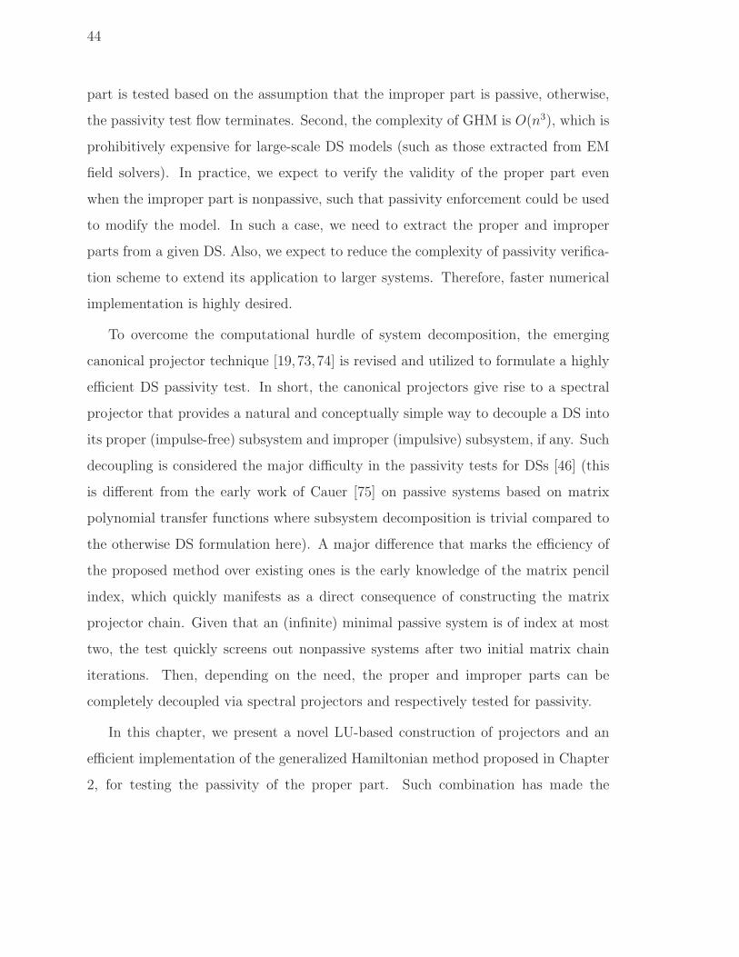
44
part is tested based on the assumption that the improper part is passive, otherwise,
the passivity test flow terminates. Second, the complexity of GHM is O(n3), which is
prohibitively expensive for large-scale DS models (such as those extracted from EM
field solvers). In practice, we expect to verify the validity of the proper part even
when the improper part is nonpassive, such that passivity enforcement could be used
to modify the model. In such a case, we need to extract the proper and improper
parts from a given DS. Also, we expect to reduce the complexity of passivity verifica-
tion scheme to extend its application to larger systems. Therefore, faster numerical
implementation is highly desired.
To overcome the computational hurdle of system decomposition, the emerging
canonical projector technique [19,73,74] is revised and utilized to formulate a highly
efficient DS passivity test. In short, the canonical projectors give rise to a spectral
projector that provides a natural and conceptually simple way to decouple a DS into
its proper (impulse-free) subsystem and improper (impulsive) subsystem, if any. Such
decoupling is considered the major difficulty in the passivity tests for DSs [46] (this
is different from the early work of Cauer [75] on passive systems based on matrix
polynomial transfer functions where subsystem decomposition is trivial compared to
the otherwise DS formulation here). A major difference that marks the efficiency of
the proposed method over existing ones is the early knowledge of the matrix pencil
index, which quickly manifests as a direct consequence of constructing the matrix
projector chain. Given that an (infinite) minimal passive system is of index at most
two, the test quickly screens out nonpassive systems after two initial matrix chain
iterations. Then, depending on the need, the proper and improper parts can be
completely decoupled via spectral projectors and respectively tested for passivity.
In this chapter, we present a novel LU-based construction of projectors and an
efficient implementation of the generalized Hamiltonian method proposed in Chapter
2, for testing the passivity of the proper part. Such combination has made the

45
proposed test truly applicable to large-scale practical DSs, as demonstrated in the
numerical section wherein the model sizes are up to 104. We also present a concise
complexity analysis of existing DS passivity tests.
3.2 DS Passivity and System Decomposition
We study a linear time-invariant (LTI) DS in the form
Ex = Ax+Bu, y = Cx+Du, (3.1)
where E,A ∈ Rn×n and B,CT ∈ R
n×m. Also, u, y ∈ Rm and x ∈ R
n are the
input, output and state vectors, respectively. The matrix E is generally singular with
rank(E) ≤ n. We assume that the matrix pencil λE−A is regular, i.e., det(λ0E−A) 6=0 for some λ0 ∈ C. Recalling from Chapters 1 & 2, we have the Weierstrass canonical
form [73]:
E = W
Iq 0
0 N
T, A = W
J 0
0 In−q
T, (3.2)
as well as the left and right (spectral) projectors, Pl and Pr, respectively, as
Pl = W
Iq 0
0 0
W−1, Pr = T−1
Iq 0
0 0
T. (3.3)

46
Given either of them, the DS transfer matrix can be decomposed as follows
G(s) =D + C(sE −A)−1B
=D − C∞B∞ + Cp(sIq − J)−1Bp︸ ︷︷ ︸Gp(s)
−sC∞NB∞ − s2C∞N2B∞ − s3C∞N3B∞ − · · ·︸ ︷︷ ︸G∞(s)
, (3.4)
where Gp(s) is the proper part (bounded as s → ∞) and G∞(s) the improper part
(unbounded as s→∞) of G(s).
If G(s) in (3.4) is viewed as
G(s) =
Gp(s)︷ ︸︸ ︷Gsp(s)︸ ︷︷ ︸
strictly proper
+M0 + sM1 +∞∑
k=2
skMk
︸ ︷︷ ︸G∞(s)
, (3.5)
then G(s) is positive real if and only if Gp(s) is positive real, M1 ≥ 0 and Mk = 0 for
k ≥ 2. Comparing (3.5) and (3.4), it is obvious that (3.1) is passive if and only if Gp(s)
in (3.4) is passive and M1 = −C∞NB∞ ≥ 0, whereas C∞N iB∞ = 0, i = 2, 3, · · · .Consequently, a key to testing the passivity of a DS is to first decouple it into its
proper and improper parts.
3.3 Matrix Projector Chain
Setting E0 := E and A0 := A, we consider a matrix chain
Ej+1 := Ej + AjQj, Aj+1 := AjPj, (3.6)
where Qj is a projector onto kerEj, i.e., Q2j = Qj and imQj = kerEj, and Pj = I−Qj
is a projector along kerEj for j = 0, 1, . . .. Obviously, PjQj = QjPj = 0. The

47
following theorem establishes the properties of the matrices Ej’s.
Theorem 3.1 [73] For a regular index-µ pencil λE−A, the matrices E0, · · · , Eµ−1
are singular, while Eµ is nonsingular.
Consequently, for the matrix chain Ej, Aj we have:
• If E1 is nonsingular, i.e., µ = 1 or N = 0, then system (3.1) is impulse-free [46].
In this case, a standard state space system can be extracted and tested for
passivity, see Section 3.4.1.
• If E1 is singular but E2 is nonsingular, we then proceed to form the spectral
projector Pr (or Pl) through constructing canonical projectors, which allows
the decoupling of G(s) into the proper and improper parts Gp(s) and G∞(s),
respectively.
• If E2 is singular, then (infinite) minimality of the DS dictates Mk 6= 0 for
k ≥ 2 [39] (see also discussion #3 in Section 3.7), so the system is nonpassive
and the passivity test is complete.
Next, we present some important properties of the matrix chain.
1. Post-multiplying the left equation in (3.6) by Qj and Pj, respectively, yields
Ej+1Qj = AjQj, (3.7a)
Ej+1Pj = Ej, (3.7b)
for j = 0, 1, · · · , µ− 1.
2. The projectors Q0, · · · , Qµ−1 are called admissible if they satisfy QjQi = 0
for j > i. Many new properties arise from using admissible projectors. For

48
example, for j = 0, · · · , µ− 1, we have
EµQj = AjQj, (3.8a)
Aj+1 = A− Eµ(Q0 + · · ·+Qj). (3.8b)
3. Canonical projectors are admissible projectors that further satisfy
Qj = QjPj+1 · · ·Pµ−1E−1µ Aj
= QjPj+1 · · ·Pµ−1E−1µ A, (3.9)
for j = 0, · · · , µ− 2, and
Qµ−1 = Qµ−1E−1µ Aµ−1 = Qµ−1E
−1µ A. (3.10)
The second equality signs in (3.9) and (3.10) can be established from (3.8b).
4. In the matrix chain (3.6), the projector Qj is, generally, not unique as only its
range is constrained. Suppose that Qj = Q2j is another projector onto kerEj.
Then QjQj = Qj, QjQj = Qj and −QjPj = QjPj. This permits a relationship
between the Ej+1’s generated by different projectors. We have
Ej+1 = Ej + AjQjQj = Ej + AjQj(I − Pj)
= (Ej + AjQj)(I + QjPj)
= Ej+1(I + QjPj). (3.11)
Provided Ej+1 is invertible, the inverse of Ej+1 is easily shown to be E−1j+1 =
(I − QjPj)E−1j+1.
The following depicts the formation of canonical and spectral projectors for the

49
non-trivial case µ = 2. Compared to [19], our presentation is highly straightforward
and the proofs in the appendices are either new or much more elegant.
3.3.1 Constructing Canonical projectors
Setting E0 := E and A0 := A, the matrix chain in the case of µ = 2 takes the form
E1 := E0 + A0Q0 and A1 := A0P0, (3.12a)
E2 := E1 + A1Q1, (3.12b)
where E2 is nonsingular. The projectors Q0 and Q1 in (3.12) are, generally, neither
canonical nor admissible, but a new matrix chain with canonical (and, therefore,
admissible) projectors can be derived from (3.12) with careful reformulation, as il-
lustrated in Appendix 3.9.1. In short, the canonical projectors Q′1 and Q′
0 can be
computed as
Q′1 = Q1E
−12 A1, (3.13a)
Q′0 = Q0P
′1E
′−12 A0 = Q0P
′1(I −Q′
1P1)E−12 A0
= Q0P′1E
−12 A0 = Q0(I −Q1E
−12 A1)E
−12 A0. (3.13b)
3.3.2 Constructing Spectral Projectors
Following from above, an important result of canonical projectors is that the right
spectral projector Pr is readily given by
Pr = P ′0P
′1 = (I −Q′
0)(I −Q′1). (3.14)

50
The proof is shown in Appendix 3.9.2. Via the expressions in (3.13) and (3.14)
[or (3.47)], it can be shown that simple analytical spectral projectors are readily de-
rived for some structured DSs [56, 77], thereby allowing fast spectral decomposition.
Nonetheless, analytical projectors generally do not exist and specific numerical consid-
erations are needed for practical spectral projector construction, as will be discussed
in Section 3.5.1.
3.4 Passivity Test
The canonical projector technique provides a natural way to decouple the proper
(impulse-free) and improper (impulsive) parts of the DS in (3.1), which translates
into a highly effective way for checking passivity based on the conditions listed af-
ter (3.5). Moreover, all that is needed is one, either the left or right, spectral projector.
Without loss of generality, we assume the availability of Pr in (3.3). The case when
Pl is available follows analogously. In the following, we see how Pr permits a sim-
ple and explicit construction of the proper and improper subsystems by the additive
decomposition procedure.
3.4.1 Additive Decomposition by Spectral Projectors
Assume that the proper part is realized by Gp(s) = C(sE − A)−1B + D. With
spectral projectors, the proper subsystem can be formed in various ways. By additive
decomposition, a regular system can be constructed explicitly as
E = EPr − A(I − Pr), A = A,
C = CPr, B = B, D = M0, (3.15)

51
where M0 is readily obtained from (3.16) below. It is straightforward to prove that E
is nonsingular by this formulation, thus no further efforts (such as SVD) are needed
to convert this DS to a regular one. To extract G∞(s) in (3.4), we first construct an
improper DS using the right spectral projector
G1(s) = D + C(I − Pr)(sE −A)−1B
= D + CT−1
0
I
sI − J
sN − I
−1
W−1B
= D − C∞B∞︸ ︷︷ ︸M0
−sC∞NB∞ − s2C∞N2B∞ − · · · . (3.16)
Contrasting (3.4) and (3.5), it follows that M1 = −C∞NB∞ which can be shown to
be
M1 = −CA−1E∞A−1B, (3.17a)
= −C(Ef + A∞)−1E∞(Ef + A∞)−1B, (3.17b)
where Ef := EPr and A∞ := A(I −Pr). Subsequently, M0 and Gp(s) can be decided
by (3.15) and (3.16). The merit of the alternative expression in (3.17b) is that the
inverse of (Ef +A∞) always exists despite the invertibility of A [or equivalently that
of J in (3.2)]. The positive semidefiniteness of M1 and M0, necessary for a passive
DS, can then be easily tested. In fact, M1 and M0 are normally small-size m × m
square matrices since the number of input/output ports is usually much fewer than
the state space dimension, i.e., m n.
At the first glance, the passivity test for Gp(s) can make use of the Hamiltonian
matrix eigenvalue test for standard state space systems [11], since E is nonsingular
such that its inverse can be absorbed into A and B (though this is sometimes not
preferable as E may be ill-conditioned). For large systems, a fast numerical approach

52
is developed [78] to compute the eigenvalues along the imaginary axis. However,
Hamiltonian-based approach becomes computationally infeasible due to the expensive
matrix inversion of E. Further, the matrix inversion also destroys the sparsity of
system matrices, which further slows down the calculations. An alternative approach
is to combine the fast eigenvalue solver of [78] with the generalized Hamiltonian
method (GHM) proposed in Chapter 2, which is further elaborated in Section 3.5.2.
This method directly tests passivity on the DS-form proper subsystem without loss
of sparsity, thus it is more efficient than using Hamiltonian method on the converted
standard state-space model.
The flow of the proposed projector-based decoupled-DS passivity test is summa-
rized in Fig. 3.1. A note about the infinite minimality assumption of the initial DS
can be found in Section 3.7 discussion #3.
3.4.2 Reconstruction into a DS
Finally, if Gp(s) = D + C(sE − A)−1B is passive (possibly after passivity enforce-
ment [11]) and M1 ≥ 0, a passive DS corresponding to the transfer function Gp(s) +
sM1 can be reconstructed for export to a simulator. Indeed, let M1 = ZZT be a
Cholesky factorization, where Z ∈ Rm×m. Then the DS can be formulated as
E
0 Im
0 0
x =
A
Im 0
0 Im
x+
B
0
ZT
u,
y =[C −Z 0
]x+ Du, (3.18)
whose transfer function is easily checked to be Gp(s) + sM1.

53
Given an infinite-minimal descriptor systemG(s)=D+C(sE-A)B
Form the matrix chain in (3.12). Find index of the matrix pencil
E,A by testing the nonsingularity of Eand E
Yes
No
No
=2 (i.e., Enonsingular)?
Form Q’and Q’ in (3.13) and P’=I-Q’, P’=I-Q’. Set
P=P’P’. Then form E=E(I-P) and E=EP
≥0?Extract the properpart G(s) as in Section 3.4.1
G(s) passive?System is passiveSystem is nonpassive
No
Yes
No
Yes
Yes
Extract the improper part G(s)=sMas in
Section 3.4.1
Test passivity of G(s) using fast GHM test or any standard regular state space technique
=1 (i.e., Enonsingular)?
Figure 3.1: Flowchart for the proposed DS passivity test in a pseudocodes style.
3.5 Implementation and Complexity
3.5.1 Fast Spectral Projector Construction
Although there exist closed-form spectral projectors in terms of the initial (not nec-
essarily canonical) projectors as in (3.13) and (3.14), or for some special cases further
simplified forms as in [56, 77], the computation can still be expensive and constitute
a bottleneck due to large-size nullspace identification, matrix multiplication and in-
verse. Here we elaborate an efficient numerical construction of spectral projectors,

54
mainly by exploiting sparsity and low-rank matrix operations inherent to many phys-
ical problems. The illustration below is based on index-2 (µ = 2) systems, and that
for index-1 (µ = 1) systems follows similarly.
First, a key step to forming the canonical projectors in (3.13) is to find the initial
projectors Q0 and Q1 spanning the nullspaces of the usually sparse or structured E0
and E1. Standard ways of identifying the nullspace include SVD or alike, which do
not utilize matrix patterns and can be expensive for large-size matrices. To this end,
we employ the sparse LU decomposition-based routine from [79], called LUQ, which
decomposes Ej, j = 0, 1, into
ETj = Lj
Uj 0
0 0
Rj, (3.19)
where Lj, Rj ∈ Rn×n are nonsingular matrices, Uj ∈ R
r×r is a nonsingular upper
triangular matrix, r is the rank of Ej and often n− r n. Therefore, (3.19) is also
used in our implementation for checking the nonsingularity of Ej. If Ej is singular, its
nullspace is then computed via the left nullspace of ETj (solely due to the reason that
Lj is produced with higher numerical accuracy than Rj by the LUQ routine [79]).
For completeness, the LUQ routine is outlined in Appendix 3.9.3. Obviously, using
I(r+1:n,:) to denote the last n − r rows of an n × n identity matrix, the columns of
(I(r+1:n,:)L−1j )T span kerEj. In practice, direct computation of this column matrix
is not preferred as the condition number of Lj can be large rendering ill-conditioned
inverse. Instead, we perform a LU factorization of Lj with permutation,
PjLj = LjUj , (3.20)
where Lj, Uj , Pj ∈ Rn×n such that Pj is the permutation matrix with P T
j Pj = I, Uj is
upper triangular and Lj is lower triangular with unit diagonal entries and a condition

55
number around unity. Then, it is easily checked that, due to the upper triangular
structure of Uj, (I(r+1:n,:)L−1j Pj)
T spans the same range as that by (I(r+1:n,:)L−1j )T
and has intrinsically better accuracy due to the low condition number of Lj. It is
noted that computing Lj does not really add to the computational load since the
inverse of Lj would generally proceed with an LU decomposition, of which Lj is a
by-product, followed by backward/forward substitutions. Next, a (modified) Gram-
Schmidt process, denoted by gs() below, leads to an orthonormal and usually thin
column matrix, namely
Ψj = gs((I(r+1:n,:)L−1j Pj)
T ), (3.21)
such that Qj = ΨjΨTj forms an orthogonal projector onto kerEj. Subsequently,
Q0 = Ψ0ΨT0 and Q1 = Ψ1Ψ
T1 are in low-rank factored forms that facilitate fast
computation of canonical projectors in (3.13) by
Q′1 := Ψ1
((ΨT
1E−12 )A1
), (3.22a)
Q′0 := Ψ0
((ΨT
0 P′1E
−12 )A0
), (3.22b)
which are again low-rank. Further computational savings can be achieved in (3.14)
by recognizing that
Q′0Q
′1 = Q′
0(Q0 + P0)Q′1
= Q0Q′1 +Q0P
′1E
′−12 A1Q
′1
= Q0Q′1 +Q0P
′1E
′−12 E ′
2Q′1 = Q0Q
′1,
so that Pr = I−Q′0−Q′
1+Q0Q′1 where Q
′0, Q
′1 and Q0Q
′1 all involve low-rank factors
only.

56
3.5.2 Fast GHM Test for Proper-Part Passivity
The spectral projector, with efficient implementation as above, allows fast decoupling
of the proper and improper parts of a DS. However, the computational bottleneck for
the DS passivity test still lies in testing the passivity of the proper part. To speed up
the overall DS passivity test, having an efficient test for the proper part is important.
For the DS-form proper subsystem constructed by (3.15), its passivity can be assessed
by the matrix pencil (J ,K) according to GHM in Chapter 2
J =
A− B(D + DT )−1C −B(D + DT )−1BT
CT (D + DT )−1C −AT + CT (D + DT )−1BT
, K =
E 0
0 ET
,
(3.23)
any purely imaginary generalized eigenvalue of which pinpoints a crossover point of
passivity violations. The proper part is strictly passive if and only if D+ DT > 0 and
(J ,K) has no eigenvalues on the imaginary axis. This eigenvalue problem consumes
an O((2n)3) complexity, which is infeasible for large sparse system. In practice, the
system matrices of Gp(s) are normally sparse, and only results close to the imaginary
axis are wanted for passivity verification. Based on this observation, the fast passivity
characterization of [78] exclusive to large sparse state-space models can be extended
to the DS case in (3.15).
To outline the fast Hamiltonian passivity test [78], we first assume the proper
subsystem is a standard state-space model. In this case eig(J ,K) = eig(J ) where Kreduces to an identity matrix. In [78], the imaginary eigenvalues of J is computed via
multi-shift Arnoldi iterations. This algorithm first builds a p-dimensional orthogonal
basis
Vp = [v1, v2, · · · , vp] , (3.24)

57
of the Krylov subspace
v1, (J − θI)−1v1, · · · , (J − θI)−(p−1)v1, (3.25)
(θ ∈ jR) with a randomly generated initial vector v1 6= 0. After that, a p × p
Hessenberg matrix Hp is constructed by
Hp = V Hp (J − θI)−1Vp. (3.26)
Subsequently a few largest eigenvalues λj of the low-dimension Hessenberg matrix
can be used to approximate the true eigenvalues λj of J close to θ by
λj ≈ θ + λ−1j . (3.27)
With an error control all λ’s close to θ can be accurately computed. To compute all
possible purely imaginary eigenvalues of J , θ should be shifted along the imaginary
axis on the upper half plane. In [78], a bisection scheme is adopted in the interval
(0, θmax) to fix the shifted parameters, such that all imaginary eigenvalues close to
θ’s are accurately found (cf. [78] for the details about error control and bisection
scheme). Here θmax is an estimated largest-magnitude imaginary eigenvalue, which
can be easily approximated by sparse power iteration. In this section, we focus on
how to extend this approach to the matrix pencil (J ,K). Note that A is assumed to
be diagonal in [78], which is waived here.
Assume λ ∈ eig(J ,K), the nonsingularity of K implies eig(J ,K) = eig(K−1J ).To apply the above fast eigenvalue solver, the main bottleneck lies in computing
(K−1J −θI)−1vi. First, (K−1J −θI) and its inverse are not sparse, which renders the
matrix-vector production inefficient. Second, the matrix inversions involved are pro-
hibitively expensive, time-consuming and unstable for large-scale systems. Therefore,

58
fast, sparse and stable matrix operations are needed. SinceK−1J−θI = K−1(J−θK),the matrix-vector production in each iteration can be expressed as
(K−1J − θI)−1vi = (J − θK)−1Kvi. (3.28)
By the matrix inverse lemma [40], we have
(J − θK)−1Kvi
=
Mθ
−MHθ
−
B
−CT
(D + DT )−1
[C BT
]
−1
wi
=
M−1
θ
−M−Hθ
wi +
M−1
θ B
M−Hθ CT
×
(D + DT − CM−1
θ B − BTM−Hθ CT
)−1 [CM−1
θ −BTM−Hθ
]wi
(3.29)
where Mθ = A − θE, wi = Kvi. We first denote wi1 = w(1:n) and wi2 = w(n+1:2n).
Making use of the sparsity of Mθ, (3.29) can be implemented as follows:
1. Perform a sparse LU decomposition on the n× n matrix
Mθ = LθUθ, (3.30)
then the sparse LU of MHθ is readily obtained as MH
θ = UHθ LH
θ .
2. Compute the following vectors (or vector-like narrow matrices)
x1 = U−1θ L−1
θ wi1, (3.31a)
x2 = −L−Hθ U−H
θ wi2, (3.31b)
x3 = U−1θ L−1
θ B, (3.31c)
x4 = L−Hθ U−H
θ CT , (3.31d)

59
by forward/backward iteration. Since Lθ and Uθ obtained by sparse LU are
normally sparse, the above linear system solution can be as cheap as O(n).
3. Finally, the inverse iteration can be computed by
(K−1J − θI)−1vi =
x1
x2
+
x3
x4
×(D + DT − Cx3 − BTx4
)−1 (Cx1 + BTx2
).
(3.32)
Due to the low dimension, the matrix inversion in this step is trivial.
In the above procedures, the total computation and storage are low since only one
n × n sparse LU factorization is needed, and only sparse upper/lower triangular
matrices and vectors are stored.
To this end, the multi-shift Arnoldi algorithm can be used to compute all gener-
alized eigenvalues of (J ,K) close to (or located on) the imaginary axis. The error
control and bisection methods are the same as those of the original algorithm [78],
which is omitted here. It is clear that compared with standard Hamiltonian method,
the GHM-based method avoids large-scale matrix inversion and preserves system
sparsity.
3.5.3 Complexity Analysis
DS passivity test by the extended positive real lemma in [39] via solution of LMIs is
impractical for large systems due to its O(n6) complexity [46] where n is the dimension
of the state vector in (3.1). Also, direct transformation to the Weierstrass canonical
form (3.2) can be numerically unstable and expensive. For example, the GUPTRI
algorithm requires essentially ≥3×SVD, ≥2×QR and 1×QZ decompositions to pro-
duce a generalized Schur form, followed by solving an additional generalized Sylvester

60
equation to reach the Weierstrass form, all costing expensive O(n3) work [80, 81].
Consequently, the more efficient SHH transformation technique is proposed [46] to
decouple the original DS into its proper and improper subsystems. A careful inspec-
tion reveals that the major SHH steps call for 3×SVD and 2×QR factorizations, plus
the optional solution of an algebraic Riccati equation (ARE) and a Lyapunov equa-
tion if the proper part is to be explicitly extracted. We are also aware of an O(n3)
DS decoupling procedure in [42, 47], which costs at least 3×URV (similar to SVD),
1×QR and one generalized Schur decomposition, and therefore has comparable com-
plexity to the SHH test (but the lack of implementation details in [42, 47] allow no
further conclusion about its actual speed). A similar procedure in [72], based on the
Van Dooren technique [82], also suffers from multiple SVDs, numerically sensitive
sub-matrix annihilations and the costly solution of an ARE. Finally, the recent DS
decoupling approach, though not exactly related to passivity test, utilizes the iterative
disk function method [83]. But again it requires 10 ∼ 20 iterations of QR factoriza-
tions (on 2n × n matrices) for convergence, followed by special subspace extraction
procedures. Another demanding requirement in all the above mentioned procedures,
where SVD/QR of dense matrices are necessary, is the O(n2) memory requirement.
After DS decoupling, either by the disk function, Weierstrass-form or SHH de-
coupling, the improper subsystem (specifically the residual M1) is then checked for
positive semidefinite which is fast and trivial. On the other hand, the proper-part
passivity can be checked with standard regular-system passivity tests such as the
Hamiltonian matrix eigenvalue test of O ((2n)3) work [11], or the faster but less reli-
able frequency sweeping test of O(m3) to O(n3) work [9] depending on the availability
of closed-form rational transfer function (e.g., a possible case where analytical trans-
fer matrix exists is when the state-space matrices are obtained from vector fitting as
in [9], but this is not always the case if the initial model is not built from rational fit-
ting). In this chapter, we directly perform GHM passivity test on the DS-form proper

61
subsystem, which is implemented by the fast multi-shift Arnoldi iteration based al-
gorithm. Assume t shift parameters in the interval (0, θmax) are used to compute all
eigenvalues close to the imaginary axis, then t sparse LUs are needed. For each shift,
several to tens of Krylov subspace iterations are needed to approximate the neigh-
borhood eigenvalues, which depends on how dense these eigenvalues are distributed.
In practice, only a small number of eigenvalues are distributed around the imaginary
axis, so usually t is in the tens. Since the expensive matrix inversion is avoided and
sparsity is preserved, this method is much more efficient than standard Hamiltonian
test on the standard state-space model converted from (3.15).
It is seen that all the above DS decomposition/decoupling approaches require at
least SVD or iterative QR operations which can of course be employed for the matrix
chain formation and projector construction in Section 3.3 (e.g., [20]). Nonetheless, a
key advantage of the projector-based DS passivity test is that the singularity test and
spectral projector formulation can all be accomplished with the much cheaper LU-
type decomposition, with ≈ O(2n3/3) work versus ≈ O(20n3) in SVD or ≈ O(2n3)
in QR for general dense matrices [40], as described in Section 3.5.1. If sparsity
and low-rank operations are further exploited, the projector can be realized with
O(n2) ∼ O(n3) work and O(n) storage, depending on the sparsity extent. In fact, for
index-2 problems, the main load in the projector construction involves only 5×sparseLU factorizations (viz. 3 rank tests and 2 nullspace computations). Subsequently,
sparsity-aware LU factorization has much reduced memory storage requirement than
the SHH or transformations to the Weierstrass form, where dense SVD, QR or matrix
equation solves are generally unavoidable. Together with the fast GHM passivity test
in Section 3.5.2, the proposed DS passivity test features remarkable computational
savings and is applicable to large systems, as will be seen in the following numerical
examples.

62
3.6 Numerical Examples
In this section, some practical DS benchmarks are tested for passivity to demonstrate
the effectiveness of the proposed projector framework. These examples are mostly
taken from [84] except the order-1232 and order-10082 ones which are RC networks.
The order-480 system is a patch antenna model from partial element equivalent circuit
(PEEC) modeling, while other higher order examples are MNA benchmarks. All
MNA benchmarks are passive, while the PEEC model is nonpassive. Nonpassive
PEEC models may be caused by poor meshing generation, inadequate numerical
integration, matrix sparsification or inappropriate geometrical discretization, which
is discussed in detail by J. Ekman, et al [85]. All codings are done in MATLAB and
executed on a 2.66GHz PC with 2GB memory.
3.6.1 Projector-Based Decomposition
We begin by timing the index tests based on checking the nullities of E1 and E2
[via (3.19)] of these benchmarks, which forms the initial step in the proposed DS
passivity test. Two approaches are contrasted, namely, the standard SVD and the
(sparse) LU singularity test discussed in Section 3.5.1. Expectedly, Table 3.1 shows
that the LU way is much more efficient than the SVD approach even though in some
cases the sparsity of E2 may not be significant due to the “fill-ins” by matrix chain
formation.
Table 3.1: Total CPU times in DS index checksystem system number of nonzero elements in time (sec)order index A0 E0 E1 E2 SVD LU
480 2 1346 (0.584%) 18290 (7.94%) 19001 (8.25%) 71521 (31.04%) 2.411 0.8125578 2 1694 (0.507%) 25432 (7.61%) 26601 (7.96%) 224130 (67.09%) 4.506 2.8231980 2 2872 (0.299%) 83568 (8.70%) 85339 (8.89%) 666669 (69.42%) 20.359 12.801232 2 3634 (0.239%) 3608 (0.238%) 3610 (0.238%) 5504 (0.363%) 29.250 0.046910082 2 30184 (0.030%) 29568 (0.029%) 29570 (0.029%) 31464 (0.031%) fail 0.093810913 2 54159 (0.045%) 35904 (0.030%) 36087 (0.030%) 5385968 (4.522%) fail 93.28

63
Table 3.2: CPU times excluding proper-part passivity check
system CPU time (sec)order proposed SHH Weierstrass
480 1.73 9.53 10.92578 3.26 15.90 18.50980 14.84 75.83 95.411232 0.0625 132.2 80110082 0.1563 fail fail10913 159.68 fail fail
Next, the proposed DS passivity test is compared to the SHH [46] and the Weier-
strass tests in terms of proper and improper part decoupling, where in the Weierstrass
approach the public routine GUPTRI [80] and the SLICOT [86] generalized Sylvester
equation solver slgesg (both calling compiled Fortran routines) are employed. The
extended LMI test in [39] has been shown by [46] to be computationally impractical
and is therefore not included here.
Table 3.2 again demonstrates the superiority of the projector approach, owing to
the techniques presented in Section 3.5.1 and the reasonings in Section 3.5.3. It is
noted that the much longer time in the Weierstrass column in the order-1232 case is
due to the generation of complex entries by GUPTRI which has also been observed
in [46]. In the same example, the speed gain from the projector approach is especially
impressive (namely, four orders faster) due to the strong sparsity of the RC network.
This further highlights the efficiency of the projector approach and in particular its
suitability for electrical networks commonly used in VLSI interconnect/package mod-
eling. To confirm the accuracy of the spectral projector decoupling, we decompose the
10913×10913 example which is a 9-input-9-output system. The proper and improper
parts are extracted by additive decomposition (cf. Section 3.4). Fig. 3.2 shows the
port-2 to port-2 decoupled responses, wherein the error is in the order of 10−10 (and
similarly for other port-to-port responses).

64
10−4
10−2
100
102
104
106
108
1010
−200
−150
−100
−50
0
50
100
150
Frequency (Hz)Magnitude (dB)
(a)
Original ResponseProper PartImproper Part
10−4
10−2
100
102
104
106
108
1010
10−20
10−15
10−10
10−5
Frequency (Hz)
Absolute Error
(b)
Figure 3.2: (a) Bode plots of the original, proper- and improper-subsystem responses.(b) Error between the original system and the sum of decomposed subsystems.
3.6.2 Proper Part Testing
After the decoupling, the proper part can be tested by SHH, Weierstrass and the
proposed fast GHM method.
We continue to show the applicability of the projector-based DS passivity test at
higher system orders than those considered in [20,46], where the highest order is 800
and the SHH and Weierstrass tests consume about 350 ∼ 600s on a standard PC.
The multi-shift Arnoldi iteration based GHM test in Section 3.5.2 is adopted.
We begin with the order-480 PEEC example which is a single-input-single-output
DS. The projector-based decomposition shows that it is impulse-free. Its proper-part
is then tested by the proposed fast GHM test. Fig. 3.3 shows that some eigenvalues
of (J ,K) locate on the imaginary axis, implying that this DS is nonpassive.
The next example is the order-980 case originating from a 4-input-4-output RLC
network, which does not contain an improper part either. The proper-part admittance
transfer function is also checked by the proposed fast GHM test. Fig. 3.4 shows the
corresponding passivity test matrix pencil does not contain any purely imaginary

65
−10 −8 −6 −4 −2 0 2 4 6 8 10−15
−10
−5
0
5
10
15
Real part
Imag
inar
y pa
rt
Figure 3.3: Eigenspectrum of the generalized Hamiltonian matrix pencil (J ,K) forthe PEEC model. Only the results close to the imaginary axis are plotted.
−3 −2 −1 0 1 2 3
x 107
−8
−6
−4
−2
0
2
4
6
8x 10
4
Real part
Imag
inar
y pa
rt
Figure 3.4: Eigenspectrum of the generalized Hamiltonian matrix pencil (J ,K) forthe order-980 RLC model. Only the results close to the imaginary axis are plotted.

66
−60 −40 −20 0 20 40 60−300
−200
−100
0
100
200
300
Real part
Imag
inar
y pa
rt
(a)
−0.1 −0.08 −0.06 −0.04 −0.02 0 0.02 0.04 0.06 0.08 0.1−150
−100
−50
0
50
100
150
Real part
Imag
inar
y pa
rt
(b)
Figure 3.5: Passivity test results for the order-10913 DS model. (a) Eigenspectrumof the generalized Hamiltonian matrix pencil (J ,K). Only the results close to theimaginary axis are plotted. (b) Zoom-in of the eigenvalues with small real parts(circled in the left plot).
generalized eigenvalues. This confirms the model is passive which is expected due to
the RLC nature of the example. The third example is the 9-input-9-output order-
10913 MNA example. The improper part contains only sM1 where M1 is a diagonal
9×9 positive definite matrix. As for its proper part, Fig. 3.5 plots the GHM test
results which confirm its passivity, whereas the SHH, Weierstrass transformations
and full-size GHM test simply fail at such high orders. In Chapter 2, the superiority
of GHM over SHH and Weierstrass tests has been illustrated. We further show the
speedup of the proposed fast GHM over the full-size GHM in Table 3.3. The CPU
timing shows the speedup of the proposed Arnoldi iteration based GHM (fast GHM)
is faster than full-size GHM, and the speedup is more significant as problem size
grows. Due to the expensive storage requirement, full-size GHM is not applicable
to large sparse systems, but the proposed fast GHM algorithm can still be used to
characterize passivity.

67
Table 3.3: CPU times of full-size GHM and fast GHM tests on the proper subsystem.
system order full-size GHM fast GHM speedup
480 21.3s 7.3s 2.9980 83.7s 15.2s 5.610913 fail 11hrs 37min N/A
3.7 Discussions
1. Compared to the Weierstrass-form or SHH-transformation DS passivity tests,
the proposed algorithm is conceptually simple and straightforward. As de-
scribed in Section 3.5.3, former DS passivity tests all involve expensive SVD
or QR operations for subsystem decoupling, while the projector approach only
calls for the much cheaper LU factorizations and much reduced memory re-
quirement when sparsity is exploited. To the knowledge of the authors, this
projector-based passivity test flow for DSs is by far the fastest one reported in
the literature.
2. Along the same line, the speed of the proposed projector construction (either
explicitly or implicitly as in [56]) is dependent on the sparsity degree and pat-
tern. In many real-world problems, E0 and E1 are highly sparse and therefore
the LUQ decomposition [79] is fast. If E2 is also sparse enough, the speedup
can be drastic as observed in the order-1232 & 10082 examples in Table 3.1.
Moreover, the nullities of practical E0 or E1 are usually low which lead to ef-
ficient low-rank formulation of canonical projectors and therefore the spectral
projector [cf. (3.21) and (3.22)]. This also reinforces the advantageous use of
projector techniques in analyzing real-world DSs.
3. Existing DS passivity tests [16, 39, 42, 46, 47] all assume a a minimal (i.e., com-
pletely controllable and observable) initial DS, otherwise a pre-processing is
done to remove the uncontrollable/unobservable states for minimal realization

68
(e.g., by the O(n3) algorithm in [3] or [46] which essentially reduces a DS into its
Kalman canonical form using orthogonal transformations). However, such pre-
processing is expensive and destroys sparsity of the system. In fact, Theorem 3.3
holds under the only assumption of regularity, and what we really require in the
DS is the infinite minimality equivalent to rank[E B
]= rank[ ET CT ] =
n [39] which determines the highest power of s in (3.5). Such infinite mini-
mality can be obtained by running the reduction algorithms in [3, 46, 72] only
partially and is therefore much cheaper to achieve than full minimality. Conse-
quently, the minimality assumption in the proposed test is the least restrictive
one among existing tests.
4. By virtue of the explicit formulation of regular state spaces for the proper and
improper subsystems in Section 3.4, further processing can be readily exer-
cised. In particular, standard state-space MOR and/or passivity enforcement
procedures, e.g., [9, 11,26], are all reusable on the extracted proper part Gp(s).
Perturbation of the improper part G∞(s) into a positive semidefinite first-order
residue matrix M1, due to its small size (viz. m×m), is also trivial.
5. In Chapter 2, GHM is directly performed on DS models for passivity check.
However, it terminates if the improper part is nonpassive, and then the pas-
sivity of the proper subsystem cannot be verified. With the spectral projector
technique, the proper part can still be checked regardless of the passivity of the
improper part.
3.8 Summary
This chapter has presented a canonical projector-based passivity test for DS mod-
els commonly found in circuit modeling. Compared to the existing LMI and SHH

69
transformation approaches for testing DS passivity, the proposed test is theoreti-
cally straightforward and exhibits simple codings and superior computational speed.
The index of a DS comes at an early stage which immediately reveals the possible
passivity of a DS. Fast sparse LU-based construction of the spectral projector then
permits efficient decomposition of the DS into its proper and improper subsystems,
whose individual passivity can be efficiently evaluated with existing passivity check
techniques. State spaces for these subsystems have also been explicitly formulated
for utilization in subsequent MOR and/or passivity enforcement. A sparse LU fac-
torization approach to projector construction, together with a fast GHM algorithm
based on multi-shift Arnoldi iteration, have made possible the efficient passivity test
of high-order DSs unamendable before.
3.9 Appendices
3.9.1 Matrix Chain with Canonical Projectors
We begin by making the projector in (3.12b) canonical. This is done by replacing Q1
with
Q′1 := Q1E
−12 A1. (3.33)
To see that Q′1 is a valid projector onto kerE1, we note that Q′
1Q1 = Q1E−12 A1Q1 =
Q1E−12 E2Q1 = Q1 and Q1Q
′1 = Q′
1, which implies Q′1(= Q′2
1 ) is a projector onto the
same range as Q1. To show Q′1 and Q0 are admissible, we have Q′
1Q0 = Q1E−12 A1Q0 =

70
Q1E−12 A0P0Q0 = 0. Using Q′
1 in place of Q1, (3.12) is updated to
E1 := E0 + A0Q0 and A1 := A0P0, (3.34a)
E ′2 := E1 + A1Q
′1. (3.34b)
Note that again E ′2 is guaranteed to be nonsingular. Now to verify the canonicity of
Q′1 in (3.34b), we make use of the property in (3.11) to get E ′
2 = E2(I + Q′1P1) and
have
Q′1E
′−12 A1 = Q′
1(I −Q′1P1)E
−12 A1
= Q′1Q1E
−12 A1 = Q1E
−12 A1 = Q′
1, (3.35)
thus completing the proof. Next, we set
Q′0 := Q0P
′1E
′−12 A0. (3.36)
Noting A0Q0 = E ′2Q0, it follows that Q′2
0 = Q′0 is a projector onto kerE0. Recom-
pute (3.34a) with this new projector to give
E ′1 := E0 + A0Q
′0 and A′
1 := A0P′0. (3.37)
Again, from (3.11), E ′1 = E1(I + Q′
0P0) and it turns out Q′1 is also a projector onto
kerE ′1, namely,
E ′1Q
′1 = E1(I +Q′
0P0)Q′1 = E1(I +Q0P
′1E
′−12 A0P0)Q
′1
= E1Q′1 + E1Q0P
′1E
′−12 A1Q
′1 = 0,

71
since A1Q′1 = E ′
2Q′1. With Q′
0, (3.34) is further updated as
E ′1 := E0 + A0Q
′0 and A′
1 := A0P′0, (3.38a)
E ′′2 := E ′
1 + A′1Q
′1. (3.38b)
Because Q′1Q0 = 0, so is Q′
1Q′0 = 0 (i.e., admissible) and
Q′0Q
′1 = Q0P
′1E
′−12 A0Q
′1 = Q0P
′1E
′−12 A0(Q0 + P0)Q
′1
= Q0P′1E
′−12 E ′
2Q0Q′1 +Q0P
′1E
′−12 A1Q
′1
= Q0Q′1 +Q0P
′1E
′−12 E ′
2Q′1 = Q0Q
′1. (3.39)
This also implies P ′0Q
′1 = P0Q
′1 and A′
1Q′1 = A1Q
′1, from which a link can be found
between E ′′2 and E ′
2 as
E ′′2 = E1(I +Q′
0P0) + A1Q′1
= E ′2P
′1(I +Q′
0P0) + E ′2Q
′1 = E ′
2(I +Q′0P0). (3.40)
Still, we need to show both Q′0 and Q′
1 in (3.38) are indeed canonical. Utilizing
properties (3.39), (3.40) and noting that A1 = A0P0 = A0P0P′0 = A′
1 − E ′2Q0P
′0, we
get
Q′0P
′1E
′′−12 A0 = Q′
0(I −Q′1)(I −Q′
0P0)E′−12 A0
= (Q′0 −Q′
0Q′1 −Q′
0P0)E′−12 A0
= (Q′0Q0 −Q′
0Q′1)E
′−12 A0 [cf. (3.39)]
= Q0P′1E
′−12 A0 = Q′
0 [cf. (3.36)]

72
Q′1E
′′−12 A′
1 = Q′1(I −Q′
0P0)E′−12 A′
1
= Q′1E
′−12 (A1 + E ′
2Q0P′0)
= Q′1E
′−12 A1 = Q′
1 [cf. (3.35)].
Of course, in practice, only the canonical projectors Q′0 and Q′
1 are required for
computing the spectral projectors, and the matrix chain updates from (3.12) to (3.34)
and then to (3.38) never need to be computed explicitly.
3.9.2 Spectral Projectors from Canonical Projectors
We give a constructive proof for Pr = P ′0P
′1 for the case µ = 2. This complements,
and is also in contrast to, the indirect argument towards spectral projector presented
in [19]. Taking the Weierstrass viewpoint for E0 and A0 (wherein N2 = 0) and
assuming canonical Q′0 and Q′
1, we can easily show
Q′0 = T−1
0 0
0 Q′0
T and Q′
1 = T−1
0 0
0 Q′1
T, (3.41)
where Q′0, Q
′1 ∈ R
(n−q)×(n−q) project onto kerN and ker(N + Q′0), respectively. More-
over,
N2 := N + Q′0 + P ′
0Q′1 = N + I − P ′
0P′1 (3.42)
is nonsingular due to Theorem 3.3. By canonicity,
Q′0 = Q′
0P′1N
−12 , Q′
1 = Q′1N
−12 and Q′
1Q′0 = 0. (3.43)

73
Next, we prove P ′0P
′1 = 0. First,
NN2 = N2 +NQ′0 +NP ′
0Q′1 = NQ′
1. (3.44)
Post-multiplying N−12 to (3.44) and using (3.43) we have N = NQ′
1 or equivalently
NP ′1 = 0. Next, recognizing P ′
0P′1 is a projector by itself, i.e., (P ′
0P′1)
2 = P ′0P
′1, and
post-multiplying it to (3.42), we obtain
N2P′0P
′1 = NP ′
0P′1 = NP ′
1 = 0. (3.45)
Nonsingularity of N2 then implies P ′0P
′1 = 0. Consequently, the right (spectral)
projector Pr in (3.3) is given by
Pr = P ′0P
′1 = T−1
Iq 0
0 P ′0P
′1
T = T−1
Iq 0
0 0
T. (3.46)
To obtain the left projector, canonical projectors are constructed from the matrix
chain starting instead with E0 := ET and A0 := AT . It is then easily verified that
Pl = (P ′0P
′1)
T = W
Iq 0
0 0
W−1. (3.47)
3.9.3 Outline of the LUQ Factorization
Given a sparse n× n matrix Z, the LUQ routine gives
Z = LZ
UZ 0
0 0
QZ , (3.48)

74
with LZ , UZ , QZ being nonsingular and UZ being upper triangular. In the first step
of LUQ, Z is factorized by sparse LU with permutation
Z = PL
U1 U2
0 U3
Q. (3.49)
Here P and Q are permutation matrices, L is lower triangular, U1 is an upper tri-
angular matrix with nonzero diagonal elements, U3 ∈ Rs×s is a very sparse upper
triangular matrix with zero diagonals, and U2 is a nonzero matrix. The zero/nonzero
diagonal elements can be distinguished by setting a small numerical threshold as
adopted in economic SVD in Matlab. Denoting L :=[L1 L2
]and Q :=
Q1
Q2
,
(3.49) can be rewritten as
Z = P[L1 L2
]U1 0
0 U3
Q1 + U−1
1 U2Q2
Q2
. (3.50)
If U3 (which is normally of low dimension if Z has a low nullity) has nonzero elements,
we can recursively perform LUQ on this block such that
U3 = LU3
UU3 0
0 0
QU3
, (3.51)
with UU3 being a nonsingular upper triangular matrix. Then LZ , UZ and QZ in (3.48)
can be decided by
LZ =[PL1 PL2LU3
], (3.52a)
UZ =
U1 0
0 UU3
, (3.52b)

75
QZ =
Q1 + U−1
1 U2Q2
QU3Q2
. (3.52c)
The cost of LUQ mainly comes from the sparse LU of Z, since U3 is highly sparse and
of low dimension. From (3.52) it is clear that LZ is a product of a permutation matrix
and a sparse lower triangular matrix. Nevertheless, QZ might be full and inaccurate
since U−11 is involved. That is why we perform LUQ on ET
j (see (3.19)) to construct
the null space of Ej.

Chapter 4
S-Parameter Generalized
Hamiltonian Methods (S-GHMs)
This chapter extends the generalized Hamiltonian method (GHM) and its half-size
variant (HGHM) to their S-parameter counterparts (called S-GHM and S-HGHM,
respectively), for testing the passivity of S-parameter descriptor-form models widely
used in high-speed circuit and electromagnetic (EM) simulations. The proposed meth-
ods are capable of accurately detecting the possible nonpassive regions of descriptor-
form models with either scattering or hybrid (impedance or admittance) transfer
matrices. Their effectiveness and accuracy are verified with several practical exam-
ples. The S-GHM and S-HGHM methods presented here provide a foundation for the
passivity enforcement of S-parameter descriptor systems (DSs).
4.1 Introduction
The transfer matrix of a LTI system may represent the admittance, impedance or
scattering parameters in the frequency domain. The admittance/impedance case has
been discussed in Chapters 2 & 3. In high-frequency applications where the electrical
76

77
variables behave like waves, scattering parameters are more commonly used, due to
their relative ease of measurement. Besides its wide application in EM simulation,
measured or simulated scattering parameters may also be used to build compact
macromodels by data fitting techniques, such as vector fitting [48] that constructs
standard state-space macromodels. Recently, the Loewner matrix interpolation tech-
nique [49, 50] has been advocated to fit measured/simulated data of electronic cir-
cuits/systems to produce the corresponding DS. Such framework is superior to the
traditional vector fitting approach in the sense that no manual pole initialization
is needed and that the optimal model order can be automatically extracted. For
these S-parameter models, passivity is crucial for stable simulation, thus passivity
verification and enforcement are needed to preserve model validity [8–12].
For DS models, several algebraic passivity tests have been proposed for hybrid
(admittance or impedance) cases [39, 42–44, 46, 47]. However, their expensive com-
putation [39] and requirements of minimal or admissible [42–44, 46, 47] realizations
render them impractical for general DS models. Moreover, due to their inability to
locate DS nonpassive regions, they are not good choices for passivity enforcement
flows. To address this problem, the frequency sweeping technique has been extended
to DS cases [20, 41]. However, due to the sampling nature of frequency sweeping, no
guarantee can be made for the complete identification of all nonpassive regions. In
Chapters 2 & 3, the proposed GHM/HGHM test delivers as high a numerical accu-
racy (of locating all nonpassive frequency intervals) for DSs as that of Hamiltonian
methods [10–14] for regular state spaces.
In the context of S-parameter DSs, passivity verification is still not well addressed.
Although the extended bounded-real lemma [45] and GARE-based method [77] have
been proposed for passivity check, no reliable technique exists for the nonpassive re-
gion identification. Due to the lack of reliable S-parameter DS passivity verification
algorithms, passivity enforcement can not be performed for nonpassive models at

78
present. Motivated by this demand, this chapter extends the GHM and HGHM theo-
ries to their S-parameter counterparts called the S-GHM and S-HGHM, respectively,
to verify the passivity of the S-parameter models in circuit or EM simulation.
4.2 Review of Passivity Check for S-Parameter Mod-
els
We consider the continuous linear time-invariant (LTI) S-parameter DS model [de-
noted by Σ : (E,A,B,C,D)], with the state-space equations
Ex = Ax+Bu, y = Cx+Du. (4.1)
Here E,A ∈ Rn×n, B ∈ R
n×m, C ∈ Rm×n, D ∈ R
m×m, and x ∈ Rn represents the state
variables. In this DS, rank(E) ≤ n and the matrix pencil (A,E) is assumed to be
regular, i.e., det(A− sE) 6= 0 for some s ∈ C. If E is full-rank (or invertible), the DS
reduces to a regular system which can be converted to a standard state-space equation
by absorbing E−1 into A and B. To distinguish from the admittance/impedance cases,
we use S(s) to denote the S-parameter transfer matrix
S(s) = C(sE − A)−1B +D. (4.2)
Recalling from Chapter 1.3.1, the (strict) passivity of the S-parameter DS (4.1) is
equivalent to the (strict) bounded realness of S(s) (s = δ + jω, where δ, ω ∈ R), i.e.,
1. S(s) is analytic on the open right half plane Re(s) > 0);
2. I − S∗(jω)S(jω) ≥ 0 (> for strict bounded realness) for all ω.

79
The second condition implies σ1 (S(jω)) ≤ 1 (or < 1 for strict bounded realness),
which can be checked by sampling some points (frequencies) along the imaginary axis
s = jω [8, 9, 41]. However, erroneous results may be obtained if nonpassive regions
between sampling points are missed. For standard state-space models (A,B,C,D)
[with E = I in (4.1)], the more reliable Hamiltonian method is preferred. The corre-
sponding 2n× 2n Hamiltonian matrix for S-parameter standard state-space model is
defined as
M =
A−BDT S−1C −BR−1BT
CT S−1C CTDR−1BT − AT
(4.3)
where S = (DDT − I) and R = (DTD − I). Since any purely imaginary scalar
jω ∈ λ(M) pinpoints a crossover point ω (in rad/sec) of passivity violations, the
(possible) nonpassive regions can be accurately located by the imaginary eigenvalue
calculation of M. To speed up calculation, [13] has further developed a half-size
singularity matrix for symmetric standard state-space models:
P =(A−B(D − I)−1C
) (B(D + I)−1C − A
). (4.4)
It has been proved that ω is a crossover point of passivity violation if and only if β
is an eigenvalue of P , where β(∈ R) = ω2 > 0. Since P ∈ Rn×n and the eigenvalue
computation has O(n3) complexity, the half-size singularity test is about 8× faster
than the full-size Hamiltonian method. Both of them are reliable but only applicable
to standard state-space models. Besides that, another limitation of Hamiltonian-
based passivity test is that (4.3) [or (4.4)] requires I−DTD (or I−D2 for symmetric
cases) to be nonsingular, which is not guaranteed in all cases.

80
4.3 S-GHM and S-HGHM
In this section we present the S-parameter GHM theories, which characterize the norm
of S(jω) and thus could be utilized for reliable passivity assessment of S-parameter
DSs. For symmetric DSs, a half-size matrix pencil can be derived to characterize the
bounded realness of an S-parameter model.
4.3.1 S-Parameter GHM (S-GHM) Theory
Theorem 4.1: Given the DS (4.1), assume that jω is not a system pole [i.e.,
jω /∈ λ(A,E)] and γ is not a singular value of D [i.e., γ /∈ σ(D)], then γ is a
singular value of S(jω) if and only if jω is a generalized eigenvalue of the matrix
pencil (M,N). The size-2n matrix pencil is defined as
M =
A−BDTS−1C −γBR−1BT
γCTS−1C −AT + CTDR−1BT
, N =
E
ET
(4.5)
where S = DDT − γ2I and R = DTD − γ2I. It is trivial to prove that M is a
Hamiltonian matrix.
Proof: Since the system matrices are real, we have S∗(jω) = BT (−jωET −AT )−1CT + DT . Assuming γ ∈ σ(S(jω)) and γ /∈ σ(D), singular value decompo-
sition (SVD) implies that there exist non-zero vectors v and u such that S(jω)u = γv
and S∗(jω)v = γu, i.e.,
[C(jωE − A)−1B +D
]u = γv,
[BT (jωET + AT )−1(−CT ) +DT
]v = γu.

81
The above relationship can be reformulated as the compact matrix form
C
BT
Ω−1
ω
B
−CT
uv
︸ ︷︷ ︸z
=
−D γI
γI −DT
uv
. (4.6)
Here
jωE −A
jωET +AT
has been denoted by Ωω. Because γ is not a singular
value of D, it is straightforward to prove that
−D γI
γI −DT
is a nonsingular matrix,
thus no non-zero vectors are contained in its null space. Since neither u nor v is zero,
the right-hand side of (4.6) is non-zero, which further implies z is a non-zero vector
[since it is a factor of the left-hand side of (4.6)]. Pre-multiplying both sides of (4.6)
by
B
−CT
−D γI
γI −DT
−1
would lead to
B
−CT
−D γI
γI −DT
−1 C
BT
z = Ωωz. (4.7)
Because
M − jωN =
B
−CT
−D γI
γI −DT
−1 C
BT
− Ωω
(4.7) can be rewritten as
Mz = jωNz. (4.8)
Therefore, jω is a purely imaginary generalized eigenvalue of the matrix pencil (M,N).
To prove the converse, we define
z′ =
−D γI
γI −DT
−1 C
BT
z =
u′
v′
(4.9)

82
which is a factor for the left-hand side of (4.7). Here u′, v′ ∈ Cn. Because Ωω is
nonsingular and z 6= 0, the right-hand side of (4.7) and thus z′ should be non-zero
vectors. Pre-multiplying (4.7) by
C
BT
Ω−1
ω would lead to
C
BT
Ω−1
ω
B
−CT
z′ =
−D γI
γI −DT
z′. (4.10)
From (4.10), one can easily get S(jω)u′ = γv′ and S∗(jω)v′ = γu′. Because neither
u′ nor v′ is zero (otherwise z′ should be a zero vector), γ is a singular value of S(jω).
4.3.2 S-Parameter HGHM (S-HGHM) for Symmetric DSs
Theorem 4.2: Assume the S-parameter DS (4.1) is symmetric [i.e., ST (jω) =
S(jω)], jω is not a generalized eigenvalue of (A,E) and γ is not a singular value of
D, then γ is a singular value of S(jω) if and only if β = ω2 > 0 is a generalized
eigenvalue of the half-size matrix pencil
(Mh, Nh) =(X + Y,E(Y −X)−1E
)(4.11)
with X and Y defined as
X = A− BDS−1C, Y = −γBR−1C. (4.12)
Proof: If the S-parameter transfer matrix of DS (4.1) is symmetric, we have
S∗(jω) = S(−jω) = C(jωE + A)−1(−B) +D. (4.13)

83
Consequently, ET , AT , BT , CT and DT in (4.5) can be replaced by E,A,C,B and
D, respectively. The following congruence transform on (M,N) gives a new matrix
pencil
(M ′, N ′) =
I I
I −I
(M,N)
I I
I −I
=
2X − 2Y
2X + 2Y
,
2E
2E
.
(4.14)
An important property of the above nonsingular congruence transform is that: jω
is a generalized eigenvalue of (M ′, N ′) if and only if it is a generalized eigenvalue of
(M,N). As we have proved the equivalence of jω ∈ λ(M,N) with γ ∈ σ (S(jω)) in
Section 4.3.1, jω should also be a generalized eigenvalue of(M ′, N ′) if γ ∈ σ(S(jω)).
In this case, det(M ′ − jωN ′) = 0, and there exist a pair of vectors w1 and w2, such
that −jωE X − Y
X + Y −jωE
w1
w2
= 0,
w1
w2
6= 0. (4.15)
Assuming X−Y being invertible, we get w2 = jω(X−Y )−1Ew1 from the upper part
of (4.15). Here w1 is nonzero (otherwise w2 is also zero). By virtue of this, (4.15)
reduces to
[Mh − ω2Nh
]w1 = 0. (4.16)
Therefore, β = ω2 ∈ λ(Mh, Nh) if γ ∈ S(jω). Analogous to S-GHM, the converse can
also be proved. Setting ω2 = jω(X − Y )−1Eω1 we can reach (4.15) from (4.16). And
then using λ(M,N) = λ(M ′, N ′) we can return to Theorem 4.1.
Note that S-HGHM only requires the DS transfer matrix S(jω) to be symmetric,
and it does not pose any restrictions on the symmetry of the system matrices.

84
0
0.2
0.4
0.6
0.8
1
Angular frequency
Sin
gula
r va
lues
of S
(jω)
(a)
1st singular value2nd singular value
0.95
1
1.05
1.1
Angular frequency
Sin
gula
r va
lues
of S
(jω)
(b)
1st singular value2nd singular value
0
0.5
1
1.5
Angular frequency
Sin
gula
r va
lues
of S
(jω)
(c)
1st singular value2nd singular value
∞ ∞ ∞
ω1
ω2
ω6
ω4
ω3
ω5
Figure 4.1: Illustrative examples for different kinds of DSs. (a) A globally strictlypassive DS. This DS has no crossover points and its transfer matrix is always unit-bounded. (b) A consistently nonpassive DS. This DS does not have any crossoverpoints, but it is nonpassive at any frequency point. (c) A DS with locally passive andnonpassive regions. This DS is nonpassive in intervals l2 = (ω1, ω2), l4 = (ω3, ω4) andl6 = (ω5, ω6).
4.4 Passivity Test of DSs
4.4.1 Passivity Test of S-Parameter DSs
In passivity test, we are interested in the special case of γ = 1, which represents the
boundary of passivity violations of an S-parameter DS. By setting γ = 1, from S-
GHM [in (4.5)] we get a passivity test matrix pencil (M,N) = (M0, N0) for scattering
DSs with
M0 =M, N0 = N. (4.17)
Here M is the Hamiltonian matrix defined in (4.3). Analogously, for symmetric
cases, from S-HGHM [in (4.11)] one can get a half-size passivity test matrix pencil
(Mh0, Nh0) defined as
Mh0 = A−B(D − I)−1C, Nh0 = E[(B(D + I)−1C − A]−1E. (4.18)
If the matrix pencil (M0, N0) (or (Mh0, Nh0) for symmetric DSs) has any purely imag-
inary (or positive real) generalized eigenvalue jω (or β = ω2), then ω is a crossover

85
frequency point where passivity violation happens.
Note that the scattering DS of interest may still be nonpassive even though no
crossover points are computed via S-GHM or S-HGHM. To further identify the pos-
sible nonpassive regions, the following procedures could be used.
1. If no crossover points are found, check S(jω0) at an arbitrarily selected fre-
quency point ω0. If ||S(jω0)|| < 1, the DS is globally strictly passive [as illus-
trated in Fig. 4.1 (a)]. Otherwise, if ||S(jω0)|| > 1 the DS is nonpassive at any
frequency point [as shown in Fig. 4.1 (b)].
2. If S-GHM/S-HGHM test produces p crossover points ω1, ω2, ..., ωp which are
increasingly ordered, one can select p + 1 sampling points ωk (k = 1, 2, ..., p +
1) such that ωk ∈ `k where `1 =(0, ω1), `i =(ωi−1, ωi) for i = 2, ..., p and
`p+1 =(ωp,∞). If ||S(jωk)|| < 1, the DS is passive in the interval `k; otherwise,
it is nonpassive in `k. An illustrative example is given in Fig. 4.1 (c).
Note that if the DS (4.1) is a regular system (when E is invertible), it can be
converted to a standard state-space model with E = I. Subsequently, for a regular
system, the generalized eigenvalue solution in the test pencil (M0, N0) can be replaced
by the standard eigenvalue computation of M0 =M. This is in fact the S-parameter
Hamiltonian passivity verification (in (4.3) of Section II-A). For symmetric regular
systems, substituting E = I into the half-size test pencil in (4.18), the generalized
eigenvalue problem reduces to the standard eigenvalue computation of P [defined in
(4.4)]. Therefore, the S-parameter Hamiltonian method and the half-size singularity
test in (4.3) and (4.4) are the subsets (or special cases) of S-GHM and S-HGHM,
respectively.

86
4.4.2 Passivity Test of Hybrid DSs
Given a square admittance or impedance transfer matrix H(s) with det(I+H(s)) 6= 0
for all Re(s) > 0, its Moebius-transformed function is defined as [77]
G(s) = (I −H(s))(I +H(s))−1. (4.19)
If I +D is invertible, a realization of G(s) = CS(sES − AS)−1BS +DS is
ES = E, AS = A−B(I +D)−1C, BS = −√2B(I +D)−1,
CS =√2(I +D)−1C, DS = (I −D)(I +D)−1.
(4.20)
Conversely, H(s) is also a Moebius-transformed function of G(s). For Moebius trans-
formation, the following properties hold [77].
1. Let H(s) = C(sE − A)−1B + D be a positive real DS transfer matrix with
nonsingular I + D, then its Moebius-transformed function G(s) is bounded
real.
2. Given a bounded real DS transfer matrix G(s) = CS(sES − AS)−1BS + DS
with I + DS being nonsingular and det(I + G(s)) 6= 0 for all Re(s) > 0, its
Moebius-transformed function H(s) is positive real.
Since D usually has a much lower dimension than E and A, the above transfor-
mation is very cheap. If we see G(s) as a scattering system, then H(s) is passive if
and only if G(s) is passive (i.e., bounded real). Therefore, we can test the passivity of
H(s) by checking the bounded realness of G(s) using S-GHM. Further, we note that
G(s) = 2(I +H(s))−1 − I (4.21)

87
Table 4.1: Applicability of different passivity tests
System model S-GHM S-HGHM Hamiltonian Half-sizemethod singularity
singular system yes yes no noregular system yes yes yes yes
asymmetric system yes no yes nosymmetric system yes yes yes yes
which implies that G(s) is symmetric if and only if H(s) is symmetric. Therefore,
S-HGHM can also be used for symmetric hybrid cases after Moebius transformation.
4.4.3 Comparison with Traditional Approaches
Table 4.1 compares the applicability of different passivity tests. There are some
distinctions among S-GHM/S-HGHM approach with traditional Hamiltonian method
and half-size singularity test.
1. S-GHM/S-HGHM can be applied to both singular and regular LTI models,
while S-parameter Hamiltonian method and half-size singularity test are only
applicable to regular systems.
2. S-HGHM and half-size singularity test are exclusive to symmetric models, but
their full-size counterparts can be used for general cases without symmetric
restrictions.
3. S-GHM and S-HGHM search for the passivity violation points via generalized
eigenvalue calculation, while traditional methods use standard eigenvalue com-
putation.
4. Due to the half-size nature, S-HGHM and half-size singularity test are 8× faster
than S-GHM and Hamiltonian test, respectively.

88
5. As will be discussed in Section 4.4.4, S-GHM/S-HGHM can test the LTI models
with I −DTD being singular, whereas the traditional approaches fail to work.
4.4.4 Numerical Issues
1. The requirement of 1 /∈ σ(D) limits the applications of Hamiltonian method
and half-size singularity test. For S-GHM and S-HGHM this restriction can be
removed after a small modification called equivalent model conversion similar to
the method in Chapter 2.4.3. The basic idea is to construct a new DS S ′(jω) =
C ′(jωE ′ − A′)−1B′ + D′, such that S ′(jω) = S(jω) and 1 /∈ σ(D′). S ′(jω)
can be constructed in different ways. In this chapter, S ′(jω) is constructed, if
necessary, as
E ′ =
E
0
, A′ =
A
I
,
B′ =
B
I
, C ′ =
[C αI −D
], D′ = αI
(4.22)
with α ∈ R and |α| 6= 1. Subsequently, the passivity of S(jω) can be checked
by performing S-GHM/S-HGHM on S ′(jω).
2. With the equivalent model conversion in (4.22), the restriction of I +D being
nonsingular in Moebius transformation can also be removed.
3. In S-HGHM passivity test, A − B(D + I)−1C is assumed to be nonsingular,
which is equivalent to 1 /∈ λ(S(0)). A proof is given in Appendix 4.8.
4. The “purely” generalized eigenvalues of (M0, N0) may appear as conjugate
pairs λk = ak ± jbk (ak, bk ∈ R). Here ak is the numerical noise induced by
the finite machine precision, which is also observed in traditional Hamiltonian

89
method [14]. A small numerical tolerance tol > 0 can be used to eliminate the
noise, and only those solutions with |ak| < tol are regarded as expected results.
The proposed passivity test is summarized in Algorithm 4.1.
4.5 Numerical Examples
This section presents some numerical examples to verify the validity and effectiveness
of S-GHM/S-HGHM for S-parameter and hybrid DSs. All examples are tested in
MATLAB R2006a on a 2.66 GHz 2G-RAM PC.
4.5.1 A Synthetic DS Model
To show the complete test flow, we consider the bounded realness of the following
order-4 single-input single-output (SISO) DS:
E =
1
1
0 1
0
, A =
−4−120
1
1
, B =
1
1
0
10−5
,
C =[10 200 10−5 0
], D = −1.
(4.23)
The transfer function of this DS is
S(jω) =10
jω + 4+
200
jω + 120− 1 + jω × 10−10. (4.24)
Solving the equation
|S(jω)| = 1 (4.25)

90
Algorithm 4.1: Passivity test by S-GHM/S-HGHM.
Input: An LTI model Σ : (E,A,B,C,D), with E,A ∈ Rn×n, B,CT ∈ R
n×m andD ∈ R
m×m.Output: The passive regions Upassive and nonpassive regions Unonpassive.begin
1. Initialization: set Upassive = Unonpassive = ∅2. if Σ : (E,A,B,C,D) is a hybrid system then
perform Moebius transform (4.20) and update Σ.
3. Compute crossover points.if 1 /∈ σ(D) and E is nonsingular then
if Σ is symmetric then
compute the crossover points by half-size singularity test (4.4);Θ← ω1, ..., ωp, where the p crossover points ω1, ..., ωp are increasinglyordered.
else
compute the crossover points by traditional Hamiltonian method (4.3);Θ← ω1, ..., ωp.
else
if 1 ∈ σ(D) thenperform equivalent model conversion (4.22), update Σ.
if Σ is symmetric then
compute the crossover points by S-GHM (4.17);Θ← ω1, ..., ωp.
else
compute the crossover points by S-HGHM (4.18);Θ← ω1, ..., ωp.
4. Locate the passive/nonpassive regionsif Θ = ∅ thencompute S(jω0) (the transfer matrix of Σ) at ω0
if ||S(jω0)|| < 1 then
Upassive = [0,∞);system is strictly passive, return.
else
Unonpassive = [0,∞);system is consistently nonpassive, return.
else`1 ← [0, ω1), `2 ← (ω1, ω2), ..., `p ← (ωp−1, ωp), `p+1 ← (ωp,∞).for i = 1, ..., p+ 1 do
compute S(jωi), with ω ∈ `i;if ||S(jωi)|| < 1 then
Upassive = Upassive ∪ `i;else
Unonpassive = Unonpassive ∪ `i.

91
we get two crossover frequency points: ω = 22.86 rad/sec and ω = 304491.7 rad/sec.
Then we use S-GHM/S-HGHM to compute the crossover points. Note that in this DS
D = −1, so we need to use equivalent model conversion in advance, which produces
an order-5 DS S ′(jω) with D′ = 0. Since the transfer function is symmetric, S-
HGHM can also be applied for passivity test. The computed results of S-GHM and
S-HGHM are listed in Table 4.2. The results of S-GHM and S-HGHM coincide with
the solutions to (4.25), which is illustrated in Fig. 4.2. Therefore, this scattering DS is
bounded real in the angular frequency band of (22.86, 304491.7), and it is nonpassive
in the bands of (0, 22.86) and (304491.7,∞).
101
102
103
104
105
106
−1
−0.8
−0.6
−0.4
−0.2
0
0.2
0.4
Angular frequency (rad/sec)
Mag
nitu
de o
f H(jω
) (d
B)
Magnitude of H(jω)Crossover points from GHM and HGHM
Figure 4.2: S-GHM and S-HGHM test results for the order-4 DS model.
Table 4.2: S-GHM/S-HGHM test results for the order-4 DS.
Imaginary results ofλ(M0, N0) (jω) Positive results of λ(Mh0, Nh0) (β)√β (rad/sec)
5.5e-7 ±j304491.7 92715196749 304491.72.05e-14 ±j22.86 522.6 22.86

92
103
104
105
106
0.2
0.4
0.6
0.8
1
1.2
1.4
1.6
Angular frequency (rad/sec)S
ingu
lar
valu
es o
f H(jω
)
(a)
1st singular value2nd singular value3rd singular valueS−GHM/S−HGHM results
103.994
103.995
103.996
0.4
0.6
0.8
1
1.2
1.4
Angular frequency (rad/sec)
Sin
gula
r va
lues
of H
(jω)
(b)
1st singular value2nd singular value3rd singular valueS−GHM/S−HGHM results
Zoom in
Figure 4.3: S-GHM and S-HGHM test results for the three-terminal filter.
4.5.2 A Symmetric S-Parameter Three-Terminal Filter
We use a three-terminal filter with symmetric port response to illustrate the appli-
cation of S-GHM/S-HGHM and the connection to their standard state-space coun-
terparts. The frequency-dependent scattering parameters are measured at 1601 sam-
pling points ranging from 50 MHz to 6 GHz. Since it is impulse-free, the input-output
response can be described by either a standard state space or a DS. To use the tradi-
tional Hamiltonian method and half-size singularity test, we first build an order-120
standard state-space model (A,B,C,D) by vector fitting [48] with 40 common poles.
Both the traditional Hamiltonian method [10] and the half-size singularity test [13]
show that this model has 9 crossover points. The imaginary eigenvalues of M and
the positive real eigenvalues of P are illustrated in the first and second columns of Ta-
ble 4.3, respectively. The obtained standard state-space model is then converted to a
DS model Hd(jω) described by (Ed, Ad, Bd, Cd, Dd), via the following transformation

93
Table 4.3: Experimental results of various passivity tests for the three-terminal filtermodel.
Hamiltonian method: Half-size singularity test: positive real S-GHM: imaginary S-HGHM: positive real results ofimaginary results of λ(M) results of λ(P)/crossover points results of λ(M0, N0) λ(Mh0, Nh0)/crossover points
6.9e-10 ±j112253 12600780132/112253 2.17e-7 ±j112253 12600780132/1122532.6e-10 ±j42988.4 18479990052/42988.4 2.58e-8 ±j42988.4 18479990052/42988.41.3e-10 ±j38173.7 14572294488/38173.7 1.06e-5 ±j38173.7 14572294488/38173.72.2e-11 ±j34551.3 1193794989.3/34551.3 2.93e-8 ±j34551.3 1193794989.3/34551.34.0e-12 ±j3109.22 9667288.145/3109.22 2.80e-6 ±j3109.22 9667288.145/3109.222.1e-12 ±j1631.07 2660378.573/1631.07 6.02e-7 ±j1631.07 2660378.573/1631.073.0e-10 ±j15871.8 251914404.4/15871.8 1.85e-8 ±j15871.8 251914404.4/15871.88.7e-11 ±j9879.71 97608669.57/9879.71 5.17e-7 ±j9879.71 97608669.67/9879.718.5e-11 ±j9895.29 97916796.34/9895.29 5.20e-7 ±j9895.29 97916796.34/9895.29
Ed =
I120
0
, Ad =
A
I3
, Bd =
B
I3
,
Cd =[C −D
], Dd = 0.
(4.26)
Then S-GHM and S-HGHM tests on Hd(jω) also give 9 crossover points shown
in the third and fourth columns of Table 4.3. Table 4.3 shows that the experimental
results of all the four methods pinpoint the same boundary frequency points, which
coincides with the singular value curves of the transfer matrix in Fig. 4.3.
4.5.3 A Symmetric Admittance PEEC Reduced Model
We use the PEEC example to show the validity of S-GHM and S-HGHM in the
passivity test of admittance or impedance DS models. This example is also used
in Chapter 2.5.2 to verify the validity of GHM/HGHM. The original SISO model is
an order-480 DS describing a patch antenna structure with admittance parameter as
its transfer function, which is obtained by partial element equivalent circuit (PEEC)
method [63]. This PEEC model is nonpassive, which may be induced by poor meshing
generation, inadequate numerical integration, matrix sparsification or inappropriate
geometrical discretization [85]. After model order reduction via PRIMA [22], an
order-53 reduced model is obtained, which is nonpassive in the low-frequency band.

94
Table 4.4: S-GHM and S-HGHM test results for the admittance reduced model (onthe Moebius-transformed system).
λ(M0, N0) (jω) λ(Mh0, Nh0) (β)√β (rad/sec)
1.309e-11 ±j0.505080 0.255103 0.5050801.307e-11 ±j0.505082 0.255110 0.5050821.127e-13 ±j1.234402 1.523749 1.2344023.650e-13 ±j2.465012 6.076287 2.4650123.169e-13 ±j2.560446 6.555922 2.5604467.587e-13 ±j4.074095 16.59825 4.074095
Since this model is a hybrid system, S-GHM and S-HGHM can not be directly
0 0.5 1 1.5 2 2.5 3 3.5 4 4.5 5−0.1
−0.05
0
0.05
0.1
Angular frequency (rad/sec)
Mag
nitu
de o
f G(jω
) (d
B)
(a)
Magnitude of G(jω)Results of S−GHM/S−HGHM
0.5051 0.5051 0.5051 0.5051 0.5051 0.5051 0.5051 0.5051 0.5051−1.5
−1
−0.5
0
0.5
1
1.5x 10
−4
Angular frequency (rad/sec)
Mag
nitu
de o
f G(jω
) (d
B) (b)
Magnitude of G(jω)Results of S−GHM/S−HGHM
Figure 4.4: S-GHM and S-HGHM test results on the Moebius-transformed transferfunction of the order-53 admittance reduced model.
used. The Moebius-transformed system is first constructed by (4.20), and then its
transfer function G(s) is tested by S-GHM and S-HGHM, respectively. The computed
crossover points are listed in Table 4.4. Fig. 4.4 shows the magnitude of the Moebius-
transformed transfer function equals unity at the computed crossover points. To show
the validity, the real part of the original admittance transfer function H(jω) is also

95
plotted in Fig. 4.5, which shows that the proposed S-GHM and S-HGHM methods
have accurately found the passivity violation points of this hybrid DS.
0 0.5 1 1.5 2 2.5 3 3.5 4 4.5 5−4
−2
0
2
4x 10
−3
Angular frequency (rad/sec)
Rea
l par
t of H
(jω)
(a)
Real part of H(jω)Results of S−GHM/S−HGHM
0.5051 0.5051 0.5051 0.5051 0.5051 0.5051 0.5051 0.5051 0.5051−4
−2
0
2
4
6x 10
−6
Angular frequency (rad/sec)
Rea
l par
t of H
(jω)
(b)
Real part of H(jω)Results of S−GHM/S−HGHM
Zoom in
Figure 4.5: The real part of the transfer function of the original order-53 admittanceDS model. The dots are the results from S-GHM and S-HGHM tests, which areaccurately located at the boundaries of passivity violations.
4.5.4 A Multi-Port DS Model
Table 4.5: CPU time (sec) comparison of S-GHM and S-HGHM.
Model Size Port Number S-GHM S-HGHM Speedup
1080 60 241.2 30.45 7.92
This example is used to verify the validity of S-GHM and S-HGHM in general
multi-port DS models, and to compare their numerical efficiency. The order-1080
symmetric DS model has 60 ports, and it is built from the measured S-parameter
data of an electronic system, via the DS-format Loewner matrix fitting [49,50]. Using
S-GHM and S-HGHM tests, 18 crossover points are obtained, which are plotted in

96
100
101
102
103
104
0
0.2
0.4
0.6
0.8
1
1.2
Angular frequency (rad/sec)S
ingu
lar
valu
es o
f S(jω)
(a)
S−GHM/S−HGHM results
101
0.96
0.98
1
1.02
1.04
Angular frequency (rad/sec)
Sin
gula
r va
lues
of S
(jω)
(b)
S−GHM/S−HGHM resultsZoom in
Figure 4.6: S-GHM/S-HGHM test results for the multi-port S-parameter DS model.The dots are the results from S-GHM and S-HGHM tests, which are accurately locatedat the boundaries of passivity violations.
Fig 4.6. Due to the large amount of crossover points, they are not listed by table.
Clearly, Fig 4.6 (b) shows that the computed results are very accurate. We have listed
the CPU times of S-GHM and S-HGHM tests in Table 4.5. It is clear that S-HGHM
is about 8× faster over S-GHM, which is expected due to its half-size nature and the
O(n3) complexity of generalized eigenvalue calculation.
4.6 Discussions
1. S-GHM and S-HGHM are purely algebraic passivity verification with similar
accuracy to Hamiltonian method and half-size singularity test. Therefore, they
are much more reliable and accurate than frequency sweeping methods, which
has been verified by their hybrid counterparts (see Chapter 2). Compared
with Hamiltonian method and half-size singularity test, S-GHM and S-HGHM
are not restricted by the restriction on D matrix, as verified by the synthetic
example.

97
2. As illustrated in Tables 4.2 to 4.4, the numerical results of S-GHM and Hamil-
tonian method contain some numerical noise in the real part, which can be
eliminated by setting a tolerance. S-HGHM and half-size singularity tests do
not suffer from this problem. From the numerical perspective, they are more
accurate over the full-size S-GHM and Hamiltonian methods.
3. Due to the half-size nature and the O(n3) complexity of (generalized) eigenvalue
computation, S-HGHM and half-size singularity test are 8× faster than their
full-size counterparts. This has been verified by the results in Chapter 2 and
the CPU timings in Table 4.5. S-GHM and S-HGHM algorithms presented here
are based on full-matrix eigensolver, so they are feasible to medium-size (e.g.,
order-1000) physical models. If we consider the Hamiltonian structure of M0
and only compute the purely imaginary roots in S-GHM test, the proposed flow
is expected to be faster and thus extensible to large and/or sparse DSs. This
work has been discussed in Chapter 3.
4. In this chapter, the passivity at the interval of two adjacent crossover points is
identified by the sampling scheme (as shown in Algorithm 4.1). An alternative
approach is to compute the slope signs of the singular value curves at the cal-
culated boundary points, according to the generalized eigenvalue perturbation
theory of Hamiltonian matrix pencils. And furthermore, using the perturbation
theory, our proposed S-GHM/S-HGHM approach also leads to a DS passivity
enforcement scheme. These issues will be reported soon in the future document.
4.7 Summary
We have extended GHM and HGHM theories of Chapter 2 to S-parameter DSs,
which reflect the relationship of the singular values of a DS transfer matrix with its

98
operating frequency. With the proposed methods, the passivity of S-parameter and
hybrid DSs can be efficiently assessed, and the passive/nonpassive regions can be
accurately located. For symmetric DSs, S-HGHM enjoys higher numerical accuracy
and an 8× speedup over S-GHM.
4.8 Appendix
In S-HGHM passivity test, the assumption of A − B(I + D)−1C is equivalent to
det[I − S(jω)] 6= 0 at the DC point (i.e., ω = 0). The proof is as follows.
Proof: Firstly, we assume that A − B(I +D)−1C is singular, then there exists a
vector p such that
[A− B(I +D)−1C]p = 0 p 6= 0. (4.27)
Since A is nonsingular, the above equation is equivalent to
A−1B(I +D)−1Cp = p. (4.28)
Denote (I + D)−1Cp by q, which should be a nonzero vector [otherwise, p 6= 0 in
(4.28)]. Pre-multiplying both sides of (4.28) by C yields
CA−1Bq = (I +D)q, q 6= 0. (4.29)
Because S(0) = D − CA−1B, (4.29) can also be written as
[I − S(0)]q = 0, q 6= 0 (4.30)
which shows I − S(0) is singular [i.e., 1 ∈ λ(S(0))].
Next, we start with (4.29) to prove the converse. Since the right side of (4.29) is
nonzero (because 1 /∈ σ(D) and q 6= 0), we denote p′ = A−1Bq which should also be

99
nonzero. Equation (4.29) is equivalent to
(I +D)−1CA−1Bq = q. (4.31)
Pre-multiplying this equation by A−1B we get
A−1B(I +D)−1Cp′ = p′, p′ 6= 0. (4.32)
Hence, A−B(I +D)−1C is singular.

Chapter 5
Fast Positive-Real Balanced
Truncation of Descriptor Systems
Modified nodal analysis (MNA) descriptions of linear VLSI circuits, such as RLC
networks, normally yield index-1 or index-2 descriptor systems (DSs) which some-
times contain improper parts. This chapter presents an improper-part preserving
passive model order reduction (MOR) procedure for RLC circuits, which consists of
two steps: additive decomposition and passive MOR on the proper subsystem. In ad-
ditive decomposition, spectral projectors are used to avoid unstable and prohibitively
expensive Weierstrass decomposition. In the passive reduction of the proper part,
we propose generalized quadratic alternating direction implicit (GQADI) iteration
and its low-rank variant (LR-GQADI) to efficiently solve the generalized algebraic
Riccati equations (GAREs). The effectiveness of the proposed algorithm is confirmed
by some practical RLC benchmarks.
100

101
5.1 Motivation
The MNA description of a RLC networks yields the LTI DS
E0x = A0x+B0u, y = C0x+D0u, (5.1)
where E0, A0 ∈ Rn×n, B0, C
T0 ∈ R
n×m , D0 ∈ Rm×m. The state vector x represents
nodal voltages, and currents flowing through voltage sources and inductors; E0 in-
cludes the capacitance and inductance terms, and A0 denotes the conductance matrix.
This DS model is widely used in interconnect [22] and power grid [24, 91] modeling.
Due to the huge size of the original DS model, linear model order reduction
(MOR) [22, 24–27, 91] is normally used to reduce the circuit complexity. When the
transfer matrix represent the admittance or impedance parameters (such as in in-
terconnect modeling), it is desired to preserve system passivity to guarantee global
stability. Typical passivity-preserving algorithms include MPVL [25] for symmetric
RC circuits and PRIMA [22] for RLC models. These Krylov-subspace projection-
based moment-matching schemes are applicable to DS models. However, they do
not give numerical error bounds. Moreover, the possible impulsive response can-
not be preserved [26]. Standard balanced truncation (BT, e.g. [28]) provides opti-
mal approximations with global error bounds, and is generally much more accurate
than Krylov-subspace projections. And the positive-real balanced truncation (PRBT,
e.g., [26, 29, 30]) can further preserve such important system properties as passivity.
However, for DS-form circuit models, a numerical transformation to the Weierstrass
canonical form [26] is required before performing BT or PRBT. By Weierstrass canon-
ical form, the possible improper part can be extracted, and the proper part is then
constructed as a standard state-space model. Unfortunately, this procedure is pro-
hibitively expensive and numerically unstable [17, 18,20].
With spectral projectors in Chapter 3, the proper and improper parts can be

102
elegantly separated [20], and standard BT and PRBT can be extended to DS models
with impulsive response [17, 18, 54]. The stability-preserving DS-BT requires solving
the (projected) generalized algebraic Lyapunov equations (GALEs), which can be
tackled by the generalized alternating direction implicit (GADI) iteration or its low-
rank variant (LR-GADI) [55,56]. To preserve passivity, DS-PRBT [17,18] solves the
(projected) generalized algebraic Riccati equations (GAREs), which utilizes Newton’s
iteration in recent literatures [17,59]. Inside each step of Newton’s iteration, one needs
to solve one (projected) GALE, so the complexity is comparable to solving tens of
GALEs, which is still expensive.
Spectral projector construction is another bottleneck with DS-PRBT flow. The-
oretically, spectral projectors can be obtained by the Weierstrass canonical form [17,
18, 54]. However, even for an order-1000 DS, computing its Weierstrass canonical
form on a general machine can be prohibitively time consuming and numerically un-
stable. An alternative approach is to use the canonical projector technique [19, 20],
which however requires expensive null space computation, matrix inversion and full
matrix-matrix products. With the special topology of RLC circuits, [18] has pro-
posed an explicit form for spectral projectors. In some cases where circuit topological
information is unavailable (e.g., for those DS models obtained by EM field solver),
the fast spectral projector construction in Chapter 3.5.1 can significantly reduce the
computational load.
In this chapter, we propose a fast PRBT-based passive MOR algorithm for DSs.
By exploiting the sparsity of circuit equations, the spectral projectors are constructed
with a low cost as in Chapter 3.5.1. The proper and improper subsystems, say, of an
RLC network, are then extracted by additive decomposition. Afterwards, the proper
part is reduced by DS-PRBT, where generalized quadratic alternating direction im-
plicit (GQADI) iteration and its low-rank version (LR-GQADI) (namely, extensions
of the QADI and LR-QADI iterative schemes in [30]) are proposed to solve the GARE

103
I (s) L
+ - V L (s)
V (s) I C (s) C
(a) (b)
Figure 5.1: (a) A C-V loop. (b) An L-I cutset.
at approximately the cost of solving only one GALE. Both system passivity and the
possible impulsive response are preserved by this DS-PRBT flow.
5.2 Preliminaries
5.2.1 Problems in DS MOR
Assume the matrix pencil (E0, A0) is regular (i.e., ∃ s0 ∈ C, det(s0E0 − A0) 6= 0),
then the DS transfer matrix reads
G(s) = D0 + C0(sE0 − A0)−1B0. (5.2)
Assuming the DS is index-µ and recalling the results from Chapters 1, 2 & 4, we
know that
G(s) = Gp(s) +Gimp(s) (5.3)
where Gp(s) and Gimp(s) are the proper and improper parts, respectively. In the time
domain, the improper part generates impulsive response. The DS in (5.1) is passive if
and only if: i) Gp(s) is positive-real; ii) Gimp(s) = sM1 where M1 = −C∞NB∞ ≥ 0.
The above DS circuit model can be reduced by either Krylov-subspace projection

104
(a) (b)
C 1
R 1
L 1
V in C 2
R 2
1 2 3
I v
I L
C 1
R 1
L 1
V in R 3
C 2
R 2
1 2 3
I L
I v
Figure 5.2: (a) An index-1 circuit without any L-V cutsets or C-V loops. (b) Anindex-2 circuit with a C-V loop formed by Vin and C1.
or PRBT. For positive semidefinite (PSD) DS, PRIMA [22] can be used to preserve
system passivity, but the improper part is normally lost. To preserve both the im-
proper part and system passivity, [26] first decomposes the original system by Weier-
strass decomposition and then uses PRBT to reduce the proper part. Unfortunately,
Weierstrass decomposition is too expensive to implement and usually numerically
unstable. Besides, the resulting proper part normally has dense and ill-conditioned
matrices, which is not preferred for ARE solvers.
5.2.2 Projected GALEs and GAREs
The projected GALEs of the DS in (5.1) are given as
AT0 XE0 + ET
0 XA0 + P Tr C
T0 C0Pr = 0, X = P T
l XPl, (5.4a)
A0Y ET0 + E0Y AT
0 + PlB0BT0 P
Tl = 0, Y = PrY P T
r . (5.4b)
Here the left and right spectral projectors
Pl = W
Iq 0
0 0
W−1, Pr = T−1
Iq 0
0 0
T, (5.5)

105
project onto the left and right deflating subspaces of (E0, A0) corresponding to their
finite eigenvalues, respectively. Some general assumptions are posed on the circuit
topologies [18]: i) there exist no loops of voltage sources or cutsets of current sources;
ii) the resistance, inductance and capacitance matrices are positive definite. Under
the above assumptions, the DS index is at most 2 (i.e., µ ≤ 2). Specifically, if no
loops consisting of capacitors and voltage sources (C-V loops) or cutsets connecting
inductors and current sources (L-I cutsets) exist, the circuit is index-1; otherwise, the
circuit is index-2 [5]. Illustrative examples are given in Figs. 5.1 & 5.2.
If (E0, A0) is stable, (5.4a) and (5.4b) have unique solutions X, Y ≥ 0. Using the
GALE (5.4b) as an example, it can be solved by the generalized ADI (GADI) [55]
(E0 + siA0)Yi− 1
2
AT0 + A0Yi−1(E0 − siA0)
T = −PlB0BT0 P
Tl , (5.6a)
(E0 + siA0)YiAT0 + A0Yi− 1
2
(E0 − siA0)T = −PlB0B
T0 P
Tl , (5.6b)
with s1, ..., si ∈ C− where C
− denotes the open left-half plane. If we set Y0 = 0, Yi
can be obtained by
Yi = −2Re(si)(E0 + siA0)−1PlB0B
T0 P
Tl (E0 + siA0)
−T+
(E0 + siA0)−1(E0 − siA0)Yi−1(E0 − siA0)
T (E0 + siA0)−T .
(5.7)
By exploiting the low-rank and positive semidefinite (PSD) properties of Yi, a low-
rank variant of GADI is further developed in [56], which significantly speeds up the
computation.

106
In DS-PRBT, one needs to get the positive-real gramians, i.e., the minimal solu-
tions X, Y (∈ Rn×n) ≥ 0 to the dual projected GAREs
ATXE + ETXA+ ETXBBTXE + P Tr C
TCPr = 0, (5.8a)
AY ET + EY AT + EY CTCY ET + PlBBTP Tl = 0, (5.8b)
such that X = P Tl XPl, Y = PrY P T
r , (E,A + BBTXE) and (ET , AT + CTCY ET )
are stable [60]. Here E = E0, M0 = D0 − C∞B∞, B = B0D,C = DTC0, A =
A0 − PlBCPr, D is defined by DDT = (M0 +MT0 )
−1. A popular method of solving
projected GARE (e.g., (5.8b)) is by Newton’s iteration (as summarized by Algo-
rithm 5.1) [18]. Inside each iteration, a (projected) GALE needs to be solved. One
can solve this (projected) GALE by GADI or LR-GADI. Obviously, solving a (pro-
jected) GARE requires solving multiple (usually tens of) (projected) GALEs.
Algorithm 5.1: Newton’s iteration for projected GARE (5.8b)
Input: E,A ∈ Rn×n, B,CT ∈ R
n×m, Pl, Pr, an initial guess Y0, and anumerical tolerance tol.
Output: The approximate solution Yi to (5.8b).begin
for j = 1,2,... doCompute Kj = EYj−1A
T and Aj = A+KjA.Solve the projected GALE: EYjA
Tj +AjYjE
T = −Pl(BBT −KjKTj )P
Tl ,
Yj = PrYjPTr .
if ||Yj − Yj−1|| < tol thenReturn Yj and exit;
elseContinue.

107
5.3 DS-MOR via DS-PRBT
The proposed DS-PRBT flow consists of two steps: i) additive decomposition that
separates the proper and possible improper parts; ii) PRBT of the proper part.
5.3.1 Additive Decomposition
We first decompose the DS by using the right spectral projector Pr (either Pr or Pl
is needed, and the procedures by using Pl are completely analogous). This chapter
considers index-2 circuits (index-1 cases are trivial [18,20]). Directly computing Pr by
Weierstrass decomposition is prohibitively expensive. From the circuit topology, Pr
can be easily obtained by its closed form [18]. If the topology is unknown, canonical
projector technique [19, 20] can be applied to compute Pr, by the sparse LU-based
fast numerical implementation elaborated in Chapter 3.5.1.
With Pr, the proper and improper subsystems can be easily separated. First, we
note
G(s) = C0(I − Pr)(sE0 − A0)−1B0 +D0
= C0T−1
0
I
sI − J
sN − I
−1
W−1B0 +D0
= C∞(sN − I)−1B∞ +D0 = Gimp(s) +M0.
(5.9)
Since the original linear RLC circuit is passive, we have Gimp(s) = sM1, then M0 and
M1 can be computed by
M0 = G(0), M1 =G(s1)− G(s2)
s1 − s2(5.10)
where s1 and s2 are positive real scalars. Subsequently, an impulse-free DS Gp(s)

108
realized by (E0,A0,B0, C0,D0) is constructed as follows:
E0 = E0Pr − A0(I − Pr) = W
Iq
−In−q
T
A0 = A0, C0 = C0Pr, B0 = B0, D0 = M0.
(5.11)
It is straightforward to prove that Gp(s) = Gp(s), E0 is nonsingular, (E0,A0) is stable.
The flow of additive decomposition is summarized in Algorithm 5.2.
Algorithm 5.2: Additive Decomposition for RLC Circuits
Input: E0, A0 ∈ Rn×n, B0, C
T0 ∈ R
n×m, D0 ∈ Rm×m
Output: E0,A0,B0, C0,M0 and M1.begin
1. Compute Pr via canonical projector technique;2. Extract M0 and M1 by (5.10), construct Gp(s) by (5.11).
5.3.2 PRBT of the Proper Subsystem
To perform passive MOR on the proper subsystem Gp(s), one needs to solve the dual
projected GAREs. Since E0 andA0 are nonsingular, the spectral projectors of (E0,A0)
are
Pl = Pr = I. (5.12)
Consequently, the projected GAREs of Gp(s) reduce to
ATXE + ETXA+ ETXBBTXE + CTC = 0, (5.13a)
AYET + EYAT + EYCTCYET + BBT = 0, (5.13b)
which are two GAREs. Here we define D by DDT = (D0 + DT0 )
−1, B = B0D,C = DTC0. A = A0−BC and E = E0. The unique PSD stabilizing solutions X and Y

109
to (5.13a) and (5.13b) are the positive real observability and controllability gramians
of Gp(s), respectively.After getting the positive real gramian matrices, the proper subsystem Gp(s) can
be balanced and reduced to a much smaller DS Gpr = Cr(sEr − Ar)−1Br +M0. The
complete DS-PRBT flow is listed in Algorithm 5.3.
Algorithm 5.3: DS-PRBT of The Proper Part
Input: A proper subsystem described by (E0,A0,B0, C0,D0), reduced order r.Output: The reduced model of Gp(s) described by (Er,Ar,Br, Cr,Dr).begin
1. Solve the dual GAREs (5.13a) and (5.13b) to get the gramians X and Y ;2. Compute the factors L and R such that X = LLT , Y = RRT ;3. Compute the skinny singular value decomposition
LTE0R =[U1 U2
] [ Σ1
Σ2
] [V1 V2
]T, where Σ1 = diag(σ1, ..., σr),
Σ2 =diag(σr+1, ..., σn) and σ1 ≥ ... ≥ σr ≥ σr+1 ≥ ... ≥ σn;
4. Compute the projection matrix: TL = Σ− 1
2
1 UT1 L
T , TR = RV1Σ− 1
2
1 ;5. Compute the reduced model of the proper part(Er,Ar, Br, Cr, Dr) = (TLE0TR, TLA0TR, TLB0, C0TR,M0);
Finally, the transfer matrix of the reduced model of the original circuit is
Gr(s) = Cr(sEr −Ar)−1Br +M0︸ ︷︷ ︸
Gpr(s)
+sM1. (5.14)
A DS realization of Gr(s) by (Er, Ar, Br, Cr, Dr) is
Er =
Er0 Im
0 0
, Ar =
Ar
Im
Im
, Br =
Br0
M1
,
Cr =[Cr −Im 0
], Dr = M0.
(5.15)
The improper part sM1 is preserved by additive decomposition without numerical
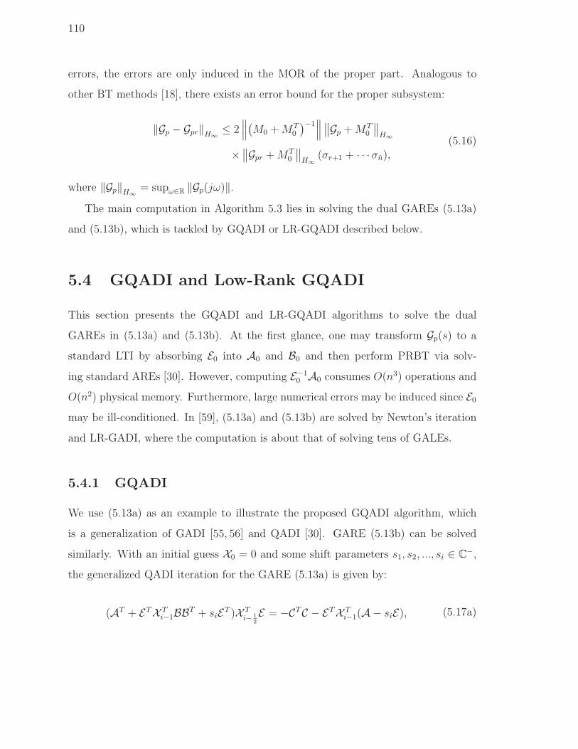
110
errors, the errors are only induced in the MOR of the proper part. Analogous to
other BT methods [18], there exists an error bound for the proper subsystem:
‖Gp − Gpr‖H∞
≤ 2∥∥∥(M0 +MT
0
)−1∥∥∥∥∥Gp +MT
0
∥∥H∞
×∥∥Gpr +MT
0
∥∥H∞
(σr+1 + · · · σn),(5.16)
where ‖Gp‖H∞
= supω∈R ‖Gp(jω)‖.The main computation in Algorithm 5.3 lies in solving the dual GAREs (5.13a)
and (5.13b), which is tackled by GQADI or LR-GQADI described below.
5.4 GQADI and Low-Rank GQADI
This section presents the GQADI and LR-GQADI algorithms to solve the dual
GAREs in (5.13a) and (5.13b). At the first glance, one may transform Gp(s) to a
standard LTI by absorbing E0 into A0 and B0 and then perform PRBT via solv-
ing standard AREs [30]. However, computing E−10 A0 consumes O(n3) operations and
O(n2) physical memory. Furthermore, large numerical errors may be induced since E0may be ill-conditioned. In [59], (5.13a) and (5.13b) are solved by Newton’s iteration
and LR-GADI, where the computation is about that of solving tens of GALEs.
5.4.1 GQADI
We use (5.13a) as an example to illustrate the proposed GQADI algorithm, which
is a generalization of GADI [55, 56] and QADI [30]. GARE (5.13b) can be solved
similarly. With an initial guess X0 = 0 and some shift parameters s1, s2, ..., si ∈ C−,
the generalized QADI iteration for the GARE (5.13a) is given by:
(AT + ETX Ti−1BBT + siET )X T
i− 1
2
E = −CTC − ETX Ti−1(A− siE), (5.17a)

111
(AT + ETXi− 1
2
BBT + siET )XiE = −CTC − ETXi− 1
2
(A− siE). (5.17b)
Similar to [30], the solution Xi can be written as:
Xi = Π(i)11 +Π
(i)12Xi−1(I − Π
(i)22Xi−1)
−1(Π(i)12 )
H (5.18a)
Π(i)11 = −2Re(si)SH
i CH(I − CS iBBHSHi CH)−1CS i, (5.18b)
Π(i)22 = −2Re(si)ES iB(I − BHSH
i CHCS iB)−1BHSHi EH (5.18c)
Π(i)12 = 2Re(si)SH
i EH − I − SHi CHCE−1Πi
22. (5.18d)
Here Si = (A+Esi)−1, and the superscript H denotes conjugate transpose. We remark
that we do not need to compute E−1 in (5.18d) since it is canceled with E in Π(i)22 .
The derivation of GQADI is detailed in Appendix 5.7.1.
5.4.2 Well Posedness
Analogous to [30], we demonstrate that the solution Xi is well defined and PSD. Since
the existence of the PSD solution X to (5.13a) implies the strict bounded realness of
the DS Σ1 : (E ,A,B, C, 0), we have
max(σ(C(A+ siE)−1B
))= max (σ(CS iB)) < 1, ∀si ∈ C
− (5.19)
where σ(o) denotes the set of singular values. Therefore, the matrix inversions in
(5.18b)–(5.18d) are well defined.
Next, we prove the well posedness of (5.18a). The GARE (5.13a) can be rewritten
as
(A+ Re(si)E)TXE + ETX (A+Re(si)E) + ETXBBTXE + CTC − 2Re(si)ETXE = 0
(5.20)

112
which implies the LTI DS Σ2 : (E2,A2,B2, C2, 0) is also strictly bounded real where
the corresponding system matrices are defined by
E2 = E , A2 = A+Re(si)E ,
B2 = B, C2 =[CT
√−2Re(si)ETZ
]H,
(5.21)
where X = ZZH . Setting ωi = −Im(si) and G2(jωi) = C2(jωiE2 − A2)−1BT
2 , the
bounded real lemma implies
max(σ(GH2 (jωi)G2(jωi))) = max(σ(BHSHi (CHC − 2Re(si)ETXE)SiB)) < 1. (5.22)
Lemma 5.1: If the GARE (5.13a) has a stabilizing solution X ≥ 0 and X ≥Xi−1, then we have X ≥ Xi.
Proof: Refer to Appendix 5.7.2.
Since X0 = 0, we have X ≥ X0. Then according to Lemma 1, X ≥ Xi follows for
i = 1, 2, · · · . Since X ≥ Xi, (5.22) can be extended to
max(σ(BHSHi (CHC − 2Re(si)ETXiE)SiB)) < 1. (5.23)
Using matrix inverse lemma [40], we get
Xi−1(I −Π(i)22Xi−1)
−1 = Xi−1[I + 2Re(si)ESiB(I − BHSHi CHCSiB)−1BHSHi EHXi−1]−1
= Xi−1
(I −
√−2Re(si)ESiB(I − BHSHi CHCSiB)−
1
2
√−2Re(si)(I − BHSHi CHCSiB)−
1
2BHSHi EH)−1
= Xi−1 − 2Re(si)Xi−1ESiB(I − BHSHi (CHC − 2Re(si)ETXi−1E)SiB
)−1BHSHi EHXi−1
(5.24)
From (5.23) and the last line of (5.24), we know that Xi−1(I − Π(i)22Xi−1)
−1 is well
defined and PSD, therefore Xi ≥ 0 is also well defined. The matrix inversion in the
last line of (5.24) is numerically easy to compute due to the low dimension.

113
5.4.3 Convergence
Now we prove that Xi indeed converges to X . Since X0 = 0, using equation (5.48) and
the star product of linear fractional transform (LFT, [4]) (see (5.40) in Appendix 5.7.1
of this chapter), ∆i = X − Xi can be formulated as a lower LFT of X :
∆i = Fl
0 Mi
MHi Ni
, X
=MiX (I −NiX )−1MH
i , (5.25a)
Mi =i∏
j=1
SHj T H
j , (5.25b)
Ni = 2Re (si)i∑
j=1
(j−1∏
k=1
SkTk)SjBBT SH
j
(j−1∏
k=1
T Hk SH
k
), (5.25c)
where Sj and Tj are defined in Appendix 5.7.2. Since si ∈ C−, −Ni ≥ 0, assume
−Ni = LiLHi and X = ZZH , then
X (I −NiX )−1 = ZZH(I + LiLH
i ZZH)−1
= ZZH(I − Li(I + LH
i ZZHLi)−1LiZZH
)
= X − ZZHLi(I + LHi ZZHLi)
−1LiZZH .
(5.26)
The last line of (5.26) shows X ≥ X (I −NiX )−1, hence
0 ≤ X − Xi ≤MiXMHi . (5.27)
Since the spectrum of SjTj locates inside the unit circle on the complex plane, Mi
approaches 0 as i increases. According to (5.27), Xi converges to X as i → ∞.
Analogous to [30,55,56], for k iterations of GQADI the shift parameters si (i = 1, ..., k)

114
can be selected by solving the minimax problem
mins1,··· ,sk∈C−
(max
λi∈spec(E,A)
∣∣∣∣(s1 − λi) · · · (sk − λi)
(s1 + λi) · · · (sk + λi)
∣∣∣∣). (5.28)
Since A = A + BBTXE (see Appendix B), directly computing spec(E , A) is not
feasible.
Lemma 5.2: Provided that X is a stabilizing solution to the GARE (5.13a), then
we have spec(E , A)=spec(K,J ) ∩ C−, where
J =
A −BBT
CTC −AT
, K =
E
ET
. (5.29)
Proof: Assume X is the stabilizing solution to (5.13a) and λ ∈ spec(K,J ) (i.e.,det(J − λK) = 0), we have
det(J − λK) = det
I
ETX I
(J − λK)
I
−XE I
= det
A+ BBTXE − λE BBT
0 −AT − ETXBBT − λET
,
(5.30)
which shows spec(K,J ) = spec(E , A) ∪ spec(−ET , AT ). Since X is a stabilizing
solution to (5.13a), we have spec(E , A) ∈ C− and spec(−ET , AT ) ∈ C
+.
By Lemma 5.2, the spectral of (E , A) can be decided as spec(K,J ) ∩ C−.

115
5.4.4 Low-Rank GQADI (LR-GQADI)
Since Xi ≥ 0, we have Xi = ZiZHi . The low-rank factor Zi is defined as
Zi =[Hi Π
(i)12Fi
]. (5.31)
Here Hi and Fi are the low-rank factors of Π(i)11 and Xi−1(I−Π
(i)22Xi−1)
−1, respectively.
Denote SCi := SHi CH , (5.18b) tells
Hi =√−2Re(si)SCi(I − SCHi BBHSCi)−
1
2 . (5.32)
Since Xi−1 = Zi−1ZHi−1, it is easy to prove that
Xi−1(I − Π(i)22Xi−1)
−1 = Zi−1(I −ZHi−1Π
(i)22Zi−1)
−1ZHi−1. (5.33)
Then Fi is decided as
Fi = Zi−1(I −ZTi−1Π
(i)22Zi−1)
− 1
2 . (5.34)
Denote SBi := SiB, the low-rank factor of Π(i)22 is expressed as
Ri =√−2Re(si)ESBi(I − SBH
i CHCSBi)− 1
2 . (5.35)
Finally, the second column block of Zi can be computed by
Π(i)12Fi = 2Re(si)SH
i EHFi −Fi
−√−2Re(si)SCiCSBi(I − SBH
i CHCSBi)− 1
2RHi Fi.
(5.36)
The procedures of LR-GQADI are summarized in Algorithm 5.4, where all computa-
tions are based on low-rank operations.
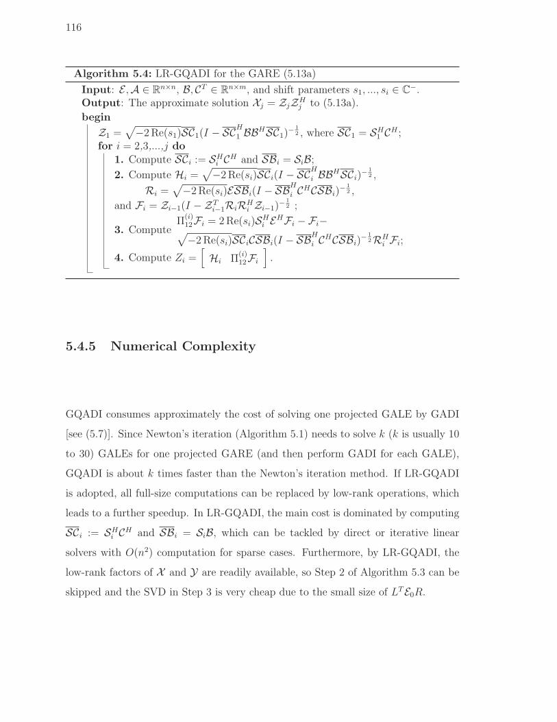
116
Algorithm 5.4: LR-GQADI for the GARE (5.13a)
Input: E ,A ∈ Rn×n, B, CT ∈ R
n×m, and shift parameters s1, ..., si ∈ C−.
Output: The approximate solution Xj = ZjZHj to (5.13a).
begin
Z1 =√−2Re(s1)SC1(I − SCH1 BBHSC1)−
1
2 , where SC1 = SH1 CH ;
for i = 2,3,...,j do1. Compute SCi := SH
i CH and SBi = SiB;2. Compute Hi =
√−2Re(si)SCi(I − SCHi BBHSCi)−
1
2 ,
Ri =√−2Re(si)ESBi(I − SBH
i CHCSBi)− 1
2 ,
and Fi = Zi−1(I −ZTi−1RiRH
i Zi−1)− 1
2 ;
3. ComputeΠ
(i)12Fi = 2Re(si)SH
i EHFi −Fi−√−2Re(si)SCiCSBi(I − SBH
i CHCSBi)− 1
2RHi Fi;
4. Compute Zi =[Hi Π
(i)12Fi
].
5.4.5 Numerical Complexity
GQADI consumes approximately the cost of solving one projected GALE by GADI
[see (5.7)]. Since Newton’s iteration (Algorithm 5.1) needs to solve k (k is usually 10
to 30) GALEs for one projected GARE (and then perform GADI for each GALE),
GQADI is about k times faster than the Newton’s iteration method. If LR-GQADI
is adopted, all full-size computations can be replaced by low-rank operations, which
leads to a further speedup. In LR-GQADI, the main cost is dominated by computing
SCi := SHi CH and SBi = SiB, which can be tackled by direct or iterative linear
solvers with O(n2) computation for sparse cases. Furthermore, by LR-GQADI, the
low-rank factors of X and Y are readily available, so Step 2 of Algorithm 5.3 can be
skipped and the SVD in Step 3 is very cheap due to the small size of LTE0R.
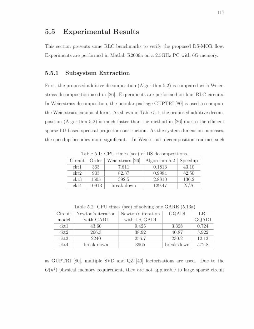
117
5.5 Experimental Results
This section presents some RLC benchmarks to verify the proposed DS-MOR flow.
Experiments are performed in Matlab R2009a on a 2.5GHz PC with 6G memory.
5.5.1 Subsystem Extraction
First, the proposed additive decomposition (Algorithm 5.2) is compared with Weier-
strass decomposition used in [26]. Experiments are performed on four RLC circuits.
In Weierstrass decomposition, the popular package GUPTRI [80] is used to compute
the Weierstrass canonical form. As shown in Table 5.1, the proposed additive decom-
position (Algorithm 5.2) is much faster than the method in [26] due to the efficient
sparse LU-based spectral projector construction. As the system dimension increases,
the speedup becomes more significant. In Weierstrass decomposition routines such
Table 5.1: CPU times (sec) of DS decompositions.
Circuit Order Weierstrass [26] Algorithm 5.2 Speedup
ckt1 363 7.811 0.1813 43.10ckt2 903 82.37 0.9984 82.50ckt3 1505 392.5 2.8810 136.2ckt4 10913 break down 129.47 N/A
Table 5.2: CPU times (sec) of solving one GARE (5.13a)
Circuit Newton’s iteration Newton’s iteration GQADI LR-model with GADI with LR-GADI GQADI
ckt1 43.60 9.425 3.328 0.724ckt2 266.3 38.92 40.87 5.922ckt3 2240 256.7 230.2 12.13ckt4 break down 3965 break down 572.8
as GUPTRI [80], multiple SVD and QZ [40] factorizations are used. Due to the
O(n2) physical memory requirement, they are not applicable to large sparse circuit

118
0 20 40 60 80 100 120 140 160 180 20010
−25
10−20
10−15
10−10
10−5
100
Han
kel s
ingu
lar
valu
es
(LR)−GQADINewton’s iteration
Figure 5.3: Approximate Hankel singular values of the proper subsystem of ckt3.Hankel singular values refer to the singular values of LTE0R (i.e., σ1, σ2, · · · in Step3 of Algorithm 5.3).
systems. The proposed method is based on sparse operations with only O(n) storage
requirement, so it is applicable to large-scale RLC circuits (as shown by the results
of ckt4).
5.5.2 Comparison of GARE Solvers
GQADI and LR-GQADI are then compared with the Newton’s iteration based GARE
solvers. We list the CPU times of solving one GARE [such as (5.13a)] in Table 5.2.
To achieve similar accuracy, the relative error is set as 10−4 for all GARE solvers.
Inside each Newton’s iteration, the relative error of solving the GALE is set as 10−6.
We remark that inside each step of Newton’s iteration, the amounts of (LR)-ADI
iterations are quite different, depending on the convergence rates of the obtained
GALEs. The CPU timing results show that GQADI and LR-GQADI enjoy significant
speedup over GADI and LR-GADI, respectively. For our tested RLC circuits, the
speedup of GQADI over LR-GADI based Newton’s iteration is case-dependent (since
the numbers of Newton’s iterations vary from case to case). For example, GQADI
is faster than LR-ADI based Newton’s iteration for ckt1 and ckt3, but it is slightly

119
10−2
100
102
104
106
108
22
23
24
25
26
27
28
29
30
31
32
Angular frequency (rad/sec)
Man
ituge
(dB
)
(a)
10−5
100
105
1010
−400
−350
−300
−250
−200
−150
−100
−50
0
50
Angular frequency (rad/sec)
Rel
ativ
e er
ror
(dB
)
(b)
originalLR−GQADINewton’s iterationPRIMA
LR−GQADINewton’s iterationPRIMA
Improper part
Figure 5.4: (a) Frequency response (port-1) of ckt3 and the reduced models (or-der=50) obtained by PRIMA and DS-PRBTs (solving the GAREs by LR-GQADIand Newton’s iteration, respectively). (b) Relative errors.
slower over the latter for ckt2. Due to the low-rank property, LR-GQADI and LR-ADI
based Newton’s method can be applied to much larger systems (shown by the last
row of Table 5.2), whereas the full-size algorithms break down due to the expensive
physical memory requirement.
5.5.3 Model Reduction Results
We continue to reduce ckt3 (with 5 ports) by DS-PRBTs (proposed DS-PRBT and
that based on Newton’s iteration [18]) and PRIMA. We first perform additive decom-
position, and then reduce the proper subsystem. Via LR-GQADI (Algorithm 5.4,
after 40 iterations) and LR-GADI based Newton’s iteration the 1505× 200 low rank
factors of X and Y (L and R in Algorithm 5.3) are obtained. Fig. 5.3 shows that
the approximate Hankel singular values (i.e., the singular values of LTE0R) decrease

120
dramatically. According to this property, the order of the reduced models is selected
as 50. Fig. 5.4(a) shows the port-1 frequency response of ckt3 and the reduced models
by various MOR methods. The results from DS-PRBT are indistinguishable from the
original response. And more importantly, the improper part is preserved by additive
decomposition. PRIMA is accurate in the low frequency band, but causes large er-
rors in the high frequency band due to the inability of capturing the improper part.
The relative error in Fig. 5.4(b) also shows the proposed DS-PRBT enjoys a higher
numerical accuracy than that based on Newton’s iteration.
−6 −4 −2 0 2 4 6
x 105
−8
−6
−4
−2
0
2
4
6
8x 10
5
Real part
Imag
inar
y pa
rt
(a)
−1500 −1000 −500 0 500 1000 1500−1
−0.8
−0.6
−0.4
−0.2
0
0.2
0.4
0.6
0.8
1
Real part
Imag
inar
y pa
rt
(b)
Figure 5.5: GHM passivity test results show that the reduced model is passive. (a)The eigenvalues of the generalized Hamiltonian matrix pencil. (b) Zoom in of thecentral part.
GHM method of Chapter 2 is used to verify the passivity of the reduced model.
The eigenvalues of the generalized Hamiltonian matrix pencil are computed and plot-
ted in Fig. 5.5. Since M0,M1 > 0 (which are preserved from the original system) and
no eigenvalues of the passivity test matrix pencil are located on the imaginary axis,
the reduced model is passive. We remark that, for symmetric DS, the passivity can
also be checked by HGHM (half-size GHM) approach presented in Chapter 2.
We note that a passive DS MOR scheme is reported in [92], which is based on

121
the PSD structure of MNA equations and solves GALEs to get the projection matrix.
However, the DS there is assumed to be regular, and practical examples show that the
method fails when a finite improper part is involved. The recently proposed dominant
spectral-zero (DSZ) interpolation [66] method reduces DS models by capturing those
poles close to the imaginary axis, however it still misses the improper parts since
the corresponding poles are located at infinity. These approaches are thereby not
compared here.
5.6 Summary
This chapter has presented a fast improper-part preserving positive-real MOR for gen-
eral DSs including RLC circuits. The proposed method first separates the proper and
improper subsystems by additive decomposition at a negligible cost, and then reduces
the proper part via solving GAREs by the newly proposed GQADI or LR-GQADI
iterative methods. The proposed algorithms are much faster than existing DS-PRBT
procedures and can capture the possible impulsive response which is normally missed
by conventional Krylov-subspace projections.
5.7 Appendices
5.7.1 Derivation of GQADI
Similar to [30], we use linear fractional transform (LFT) [4] techniques to derive the
formulation of GQADI. A lower LFT Fl(P,∆) with
P =
P11 P12
P21 P22
(5.37)

122
is defined as
Fl(P,∆) = P11 + P12∆(I − P22∆)−1P21. (5.38)
An upper LFT is defined as
Fu(Q,∆) = Q22 +Q21∆(I −Q11∆)−1Q12, (5.39)
where Q is portioned similarly to P . An important result of LFT is the star product
operation [4]:
Fl(P, Fl(Q,∆)) = Fl (W, ∆) (5.40)
with
W =
Fl(P,Q11) P12(I −Q11P22)
−1Q12
Q21(I − P22Q11)−1P21 Fu(Q,P11)
. (5.41)
From (5.17a) and (5.17b) we get
Xi− 1
2
= Fl(Pi, Xi−1), Xi = Fl(PHi , Xi− 1
2
). (5.42)
Here Pi can be decided as
Pi =
−C
H CSi CH CSiBBH − T Hi
Si SiBBH
(5.43)
with C = CE−1, Si = (AE−1 + siI)−1 = ES i and Ti = AE−1 − siI. Setting P = PH
i ,
Q = Pi and ∆ = Xi−1in (5.40), Xi can be expressed by Xi−1 via the following LFT:
Xi = Fl(Π(i),Xi−1) = Fl
Π
(i)11 Π
(i)12
(Π(i)12 )
H Π(i)22
, Xi−1
. (5.44)
The sub-blocks of Π(i) are given in (5.18b)–(5.18d).

123
5.7.2 Proof of Lemma 5.1
Proof: Set A = A + BBTXE . Since X is a stabilizing solution of (5.13a), (A, E) is
stable, and A+ siE is nonsingular for any si ∈ C−. Denoting Si := E(A+ siE)−1 and
Ti := (A − siE)E−1, it is straightforward to prove that any multiplication among Sm,Tn (m and n are any positive integers) and AE−1 is commutative.
According to (5.13a), (5.17a) can be rewritten as
ET(X − Xi− 1
2
)(A+ siE − BBT (X − Xi−1)E
)
=(AT − siET
)(X − Xi−1),
(5.45)
which implies
X − Xi− 1
2
= Fl
(Pi, X − Xi
). (5.46)
Here Pi =
0 −T H
i
Si SiBBT
. Similarly, from (5.13a) and (5.17b) we get
X − Xi = Fl
(PH
i , X − Xi− 1
2
). (5.47)
By the star product of LFT shown in (5.40), ∆i = X − Xi can be expressed as the
lower LFT with respect to ∆i−1 = X − Xi−1:
∆i = Fl
0 SH
i T Hi
TiSi 2Re (si) SiBBT SHi
, ∆i
= SHi T H
i ∆i−1
(I − 2Re (si) SiBBT SH
i ∆i−1
)−1
TiSi.
(5.48)
Denoting ∆i−1 = MiMTi and −2Re (si) SiBBT SH
i = NiNTi (since both of them are

124
PSD), matrix inverse lemma [40] shows
∆i−1
(I − 2Re (si) SiBBT SH
i ∆i−1
)−1
= MiMTi
(I +NiN
Ti MiM
Ti
)−1
= MiMTi
(I −Ni
(I +NT
i MiMTi Ni
)−1NT
i MiMTi
)
= Mi(I +MTi NiN
Ti Mi)
−1MTi ≥ 0.
(5.49)
Therefore, it is obvious that ∆i = X − Xi ≥ 0.

Chapter 6
Block-Diagonal Structured Model
Reduction for Power Grid Analysis
This chapter proposes a block-diagonal structured model order reduction (BDSM)
scheme for multi-port LTI models, with power grid as a typical example in VLSI de-
sign. Compared with existing power grid model order reductions (MORs), BDSM has
several advantages. First, unlike many power grid reductions that are based on ter-
minal reduction and thus error-prone, BDSM utilizes an exact column-by-column
(or row-by-row) moment matching scheme to provide higher numerical accuracy.
Second, with similar accuracy and macromodel size, BDSM generates very sparse
block-diagonal reduced-order models (ROMs) for massive-port systems at lower cost,
whereas traditional frameworks such as PRIMA produce full dense models rendering
inefficient simulation. Third, different from those MORs based on extended Krylov
subspace (EKS) technique, BDSM is input-signal independent, so the resulting ROM
is reusable under different excitations. Finally, due to its special structure, the ob-
tained ROM can be simulated flexibly: it can be solved either in a parallel fashion
or in a serial flow; and in the column-by-column moment-matching BDSM frame-
work, the problem size can be scaled with the active port number. The accuracy and
125

126
efficiency of BDSM are then verified by industrial power grid benchmarks.
6.1 Introduction
Power grid analysis has been a major topic in modern VLSI design. The challenges
for power grid analysis mainly stem from the large problem size and massive port
number. A typical power grid model usually has millions of nodes and up to thousands
of input sources, rendering it extremely difficult to simulate. During the past decade,
numerous efforts have been made to speed up the analysis and/or simulation of power
grid networks, such as domain decomposition technique [93], preconditioned Krylov-
subspace iterative method [94], random walk algorithm [95], simulations based on grid
locality [96], and multi-grid reduction technique [97, 98]. One issue of these methods
is that the computation on the large model needs to be repeated for different inputs
or time steps.
A viable solution is to approximate the many-port original network by MOR, and
then use the much smaller model in subsequent simulation. Krylov-subspace projec-
tions [22, 25] and balanced truncations [28] have been highly successful in intercon-
nect MOR. With some modifications, these standard techniques have been adapted
to reduce more sophisticated models in circuit simulation [33, 34]. Krylov-subspace
projections such as PRIMA [22] have superior efficiency over balanced truncations.
Therefore, they have been modified to reduce power grid models [24, 91, 100]. How-
ever, the efficiency significantly degrades as the port number increases. First, the
MOR cost increases linearly with the port number, making the computation ineffi-
cient. Second, the ROM size increases linearly with the port number, resulting in
a quadratic increase on storage cost. Consequently, the normally large and dense
ROMs make the simulation very inefficient.

127
To address the problems induced by the large port number, extended Krylov sub-
space (EKS [100]) and extended truncated balance realization (ETBR [101]) treat
the product of input vector and input matrix as a new frequency-dependent “single-
input matrix”, and then reduce a “single-input multi-output” systems. Based on a
similar idea, triangularization based structure preserving MOR (TBS [91]) generates
structured ROMs to further speed up power grid simulation. However, these meth-
ods are highly dependent on the input signals, and the obtained ROMs can not be
reused for different input patterns. Since there exist some correlations between the
input-output pairs, singular value decomposition (SVD) can be used to compress the
terminals before MOR [102]. Similarly, [103] uses frequency-dependent packing to
improve the numerical accuracy; B. Yan et al. has proposed decentralized MOR (De-
MOR [104]) for multi-port system reduction. However, the terminal reduction process
is error-prone, because the true transfer matrix moments can not be matched.
In this chapter, we present a novel method, called block-diagonal structured MOR
(BDSM), for power grid reduction subject to the following criteria:
1. The ROMs should be cheap to simulate, which means that the obtained ROM
should be compact enough or has a special structure that permits fast compu-
tation;
2. The ROMs should be reusable, which means that the ROM is accurate no
matter what kind of signal waveforms are posed on the input ports;
3. The MOR accuracy should be comparable to that of PRIMA, which means that
a certain number of moments are accurately matched in a predefined frequency
band.
By BDSM, we get ROMs having the same sizes and similar accuracy as those from
PRIMA. Even more, the models from BDSM are sparse and block-diagonal, thereby

128
facilitating fast simulation. Since BDSM does not involve terminal reduction, it is
more accurate over terminal-reduction based MOR. On the other hand, BDSM is
input-independent, so the ROMs can be reused for different input patterns. Due to
their block-diagonal structure, the ROMs can be efficiently simulated and allows for
parallel calculations. Furthermore, if we consider the active/dead inputs, the problem
size can be largely reduced, which provides further simulation speedup for power grids
with consideration of clock gating [108].
6.2 Review of Power Grid MOR
6.2.1 Power Grid Model
We consider the modified nodal analysis (MNA) equation of a power grid network
Cdx(t)
dt= Gx(t) +Bu(t), y(t) = Lx(t) (6.1)
where C,G ∈ Rn×n, B ∈ R
n×m, L ∈ Rp×n. The input vector u(t) normally rep-
resents time-varying current sources from transistor-level circuit blocks; the output
vector y(t) contains the voltage or current variables of interest; the state vector x(t)
represents nodal voltages and the branch currents across inductive components. The
system matrix C includes the capacitance and inductance terms; G denotes the
conductance matrix; B and L are the input and output matrices, respectively. In
this chapter, we focus on the cases with multiple sources, which is very common in
power/ground network models. Sometimes (e.g., in transient simulation) we may
need to solve x(t) for a given u(t). In such a case, L is set to In (a dimension-n
identity matrix), so y(t) = x(t).
Provided the matrix pencil (C,G) being regular (i.e., ∃s ∈ C such that (sC −G)

129
is nonsingular), in Laplace domain, the p×m transfer matrix can be written as
H(s) = L(sC −G)−1B. (6.2)
Due to the grounded capacitors at the input nodes, the DS models from power grid
networks are normally impulse-free. In power grid MOR, we attempt to find the left
and right projection matrices W,V ∈ Rn×q with q n, to construct a small size-q
linear system Σr : (Cr, Gr, Br, Lr)
Crdz(t)
dt= Grz(t) +Bru(t), yr(t) = Lrz(t) (6.3)
with Cr = W TCV , Gr = W TGV , Br = W TB and Lr = LV , such that Hr(s) =
Lr(sCr − Gr)−1Br ≈ H(s) or yr(s) = Hr(s)u(s) ≈ y(s), subject to some accuracy
requirements.
If W = V , the projection is a congruence transform. For simplicity, we use
congruence transform in chapter. The projection matrices can be constructed by
(rational) Krylov subspace moment matching [22, 25, 106] or balanced truncations
(BT) [28]. Although BT approaches may provide a priori error estimation, they
become inefficient for such large-scale systems as power grid networks whose problem
sizes may be in the millions. Therefore, Krylov-subspace projections are discussed in
this chapter.
6.2.2 Problems with Standard Krylov-Subspace Projection
Given a matrix M and (block) vector R with compatible sizes, an l-th order (block)
Krylov subspace Kl(M,R) is the space spanning the range of a set of (block) vectors,
i.e.,
Kl(M,R) = R,MR,M2R, · · · ,M l−1R.

130
By (block) Arnoldi algorithm [22], the projection matrices for a congruence transform
can be constructed as
W = V = Kl(s0C −G)−1C, (s0C −G)−1B (6.4)
with s0 being a specific expansion point. Then a size-q ROM with q = ml can
be constructed, such that Hr(s) matches the first l moments of H(s) around the
expansion point s0, i.e.,
H(s) = Hr(s) +O((s− s0)
l). (6.5)
If the input signals are distributed in a wide frequency band, multi-point Krylov-
subspace projection may be used to improve the numerical accuracy [106]. For exam-
ple, to match the first l moments of H(s) at k expansion points s0, s1, · · · , sk−1, the
projection matrices are constructed by the union of the Krylov subspace at each ex-
pansion point. We proceed with single-point projection, and the multi-point scheme
readily follows.
The standard projections have some problems when applied to power grid net-
works. First, the obtained ROMs are not efficient for computer-aided simulation.
Since the ROM size q increases linearly with the port number m, it is clear that the
ROM size can be very large. Since the ROM’s matrices from standard projections are
normally dense, storing the ROMs becomes challenging for a general PC, let alone
simulating the ROM. Second, the cost of projection matrix construction is high for
large many-port systems. To construct the projection matrix in (6.4), we need to
perform ml(ml−1)2
steps of long-vector orthonormalization, whose cost quadratically
increases with m. Therefore, standard moment-matching based projection would be
inefficient for power grid reduction.
Some modifications have been made for MOR of power grid networks. These

131
approaches are mainly based on terminal reduction [102–104] or the ideas similar to
extended Krylov-subspace projection [91,100,101]. The former capture the moments
of a low-rank approximated transfer matrix [102–104], rather than the original one.
Therefore, essentially the model compactness is obtained at the cost of model accu-
racy. EKS, ETBR and TBS generate compact ROMs via moment matching of the
output response under a predefined input excitation [91, 100, 101]. However, due to
their strong dependency on input signal waveforms, the ROMs need to be rebuilt
every time as the excitation vector changes. Since the cost in MOR is much more ex-
pensive over simulating a ROM, this kind of approaches may be inefficient for power
grid analysis if we need to simulate the response under different excitations.
6.3 BDSM Scheme
This section presents the proposed BDSM algorithm to generate block-diagonal struc-
tured ROMs for power grid networks. We first decompose the original MIMO (multi-
input multi-output) system into m MIMO subsystems (each with a p×m transfer ma-
trix), via input matrix splitting. Then, we show that the Krylov-subspace projection
matrix of each MIMO subsystem is in fact identical to that of a SIMO (single-input
multi-output) subsystem. To match l moments, the proposed method generates an
ml × ml ROM as by PRIMA. However, the resulting ROM’s system matrices only
contain m blocks in the diagonal, with each one being a small l × l matrix. As will
be discussed in Section 6.4, this structure makes the subsequent simulation highly
efficient. For simplicity, we only discuss the projection at a single point, and the
multi-point projection follows analogously.

132
6.3.1 Input Matrix Splitting
Denoting the i-th column of B ∈ Rn×m by bi, the input matrix can be splitted to m
rank-1 matrices, i.e.,
B =m∑
i=1
Bi, with Bi ∈ Rn×m, Bi(:, j) =
bi, if i = j
0, if i 6= j(6.6)
for i, j = 1, 2, · · · ,m. Here Bi(:, j) denotes the j-th column vector of Bi. The linear
time-invariant (LTI) system (C,G,Bi, L) is called a splitted system, denoted by Σi.
Σi’s transfer matrix is written as Hi(s) = L(sC −G)Bi. Clearly, the original transfer
matrix H(s) can be rewritten as
H(s) =m∑
i=1
Hi(s). (6.7)
Subsequently, the original network can be reformulated as the parallel connection of
Σi′s, and then realized by a size-mn model (C, G, B, L):
C =
C. . .
C
, G =
G. . .
G
B =[BT
1 · · · BTm
]T, L =
[L · · · L
].
(6.8)
This larger-size block-diagonal system is an equivalent model of the original power
grid network. Note that Hi(s) is a p ×m matrix with only one column vector (the
i-th column) being non-zero, which is identical to the i-th column of H(s).
Generally, if we attempt to match the first l moments of a general m-port size-
mn model via standard Krylov subspace projection such as PRIMA [22] at a single
expansion point, a size-ml ROM would be generated. During the projection, the

133
block-diagonal structure would be destroyed and a dense ROM would be produced,
which makes the ROM-based simulation very inefficient. Additionally, reducing a
size-mn linear system is normally much more expensive over reducing a size-n system,
since more calculations are needed in the LU decomposition, linear system solution
and Gram-Schmidt orthonormalization. In BDSM, we aim to keep the block-diagonal
structure of (6.8) such that the storage and calculations could be much cheaper in
the subsequent simulation steps. We also expect the MOR cost to be cheaper than
traditional projection frameworks on (6.1). More importantly, the resulting ROM is
expected to be reusable for repeated simulation under varying input patterns.
To proceed, we consider the i-th splitted system Σi. Excited by the input vector
u(s), the output vector is yi(s) = Hi(s)u(s), and it can be rewritten as
yi(s) = L(sC −G)−1Biu(s) = L(sC −G)−1biui(s) (6.9)
since Bi has only one nonzero vector in the i-th column. Here, ui(s) denotes the i-th
input scalar. This reformulation shows that yi(s) is only dependent on the input ui,
and Bi shields the effects induced by other input signals, although the splitted system
Σi hasm input ports. Since y(s) is the sum of yi(s) for i = 1, · · · , m, the above input
matrix splitting is physically equivalent to decomposing the output response into m
independent components, with each excited by a single input signal. This property
in fact allows for a block-diagonal structure-preserving reduction for model (6.8), at
a lower computational cost over PRIMA.
6.3.2 Block-Diagonal Structured Projection
Unlike traditional projection reduction methods that directly match the moments of
H(s), BDSM uses an indirect moment matching method. Specifically, the ROM of
each splitted model Σi, denoted by Σir, is built such that its transfer matrix Hir(s)

134
matches the first l moments of Hi(s), and then all reduced models are parallely
connected to approximate the original linear network (6.1).
Let us consider the splitted model Σi : (L,C,G,Bi). At a single expansion point
s0, a projection matrix spanning the l-th order block Krylov subspace can be con-
structed:
V (i) = Kl(s0C −G)−1C, (s0C −G)−1Bi. (6.10)
Then the ROM of Σi, denoted by Σir : (Cir, Gir, Bir, Lir), can be constructed by the
congruence transform
Cir = (V (i))TCV (i) Gir = (V (i))TGV (i)
Bir = (V (i))TBi and Lir = LV (i).(6.11)
It can be proved that the ROM’s transfer matrix Hir matches the first l moments of
Hi(s), i.e.,
Hir(s) = Lir(siCir −Gir)−1Bir = Hi(s)−O
((s− s0)
l)
(6.12)
Since Bi ∈ Rn×m, it seems that V (i) is a n×ml matrix and the size of the ROM Σir
would be ml. By noting that Bi has only one nonzero vector bi as its i-th column, it
is straightforward to prove
V (i) = Kl
(s0C −G)−1C, (s0C −G)−1bi
∈ R
n×l (6.13)
provided that no vectors are deflated in the orthonormalization steps. Therefore, V (i)
is in fact a n× l projection matrix, and Σir is a very small size-l ROM, although Σi
is an MIMO.
After computing the projection matrix for each splitted system Σi, a projection
matrix can be constructed for model (6.8). Using the congruence transform Cr =

135
VTCV , Gr = VTGV , Br = VTB and Lr = LV , the system matrices of the final ROM
of (6.8) [denoted by Σr, which is also the final ROM of (6.1)], can be decided as
Cr = blkdiag (C1r, · · · , Cmr) , Gr = blkdiag (G1r, · · · , Gmr)
Br =
B1r
...
Bmr
= blkdiag
((V (1))T b1, · · · , (V (m))T bm
)
and Lr = LV , with V = blkdiag(V (1), · · · , V (m)
).
(6.14)
Here “blkdiag” denotes the Matlab function that constructs a block-diagonal matrix
from the input arguments. It is clearly shown that the final size-ml ROM is block-
diagonal structured. All diagonal blocks of Cr and Gr (i.e., Cir and Gir for i =
1, · · · , m) are small l× l matrices. The i-th block of Br (i.e., Bir) contains only one
nonzero vector as its i-th column.
From (6.14) and (6.12), the transfer matrix of Σr can be written as
Hr(s) =m∑
i=1
Hir(s) = H(s)−O((s− s0)
l). (6.15)
Therefore, Hr(s) matches the first l moments ofH(s), and BDSM has similar accuracy
to PRIMA [22]. In PRIMA, the first l moments of H(s) are matched in a matrix
format. However, in BDSM, each p × m transfer matrix Hir(s) captures the first l
moments of H(s)’s i-th column. Consequently, their sum, Hr(s), captures H(s)’s first
l moment matrices in a column-by-column style, as illustrated in the BDSM flow of
Fig 6.1.
6.3.3 Numerical Complexity
The detailed implementation is presented in Algorithm 6.1. Assume that no vectors

136
H(s)
H 1 (s)
H i (s)
H m (s)
H 1r (s)
H ir (s)
H mr (s)
+ = H r (s)
non-zero vector in H i (s) or H(s)
zero vector in H i (s) or H ir (s)
non-zero vector in H ir (s) or H r (s)
MOR
MOR
MOR
. . .
. . .
... ...
... ...
... ...
... ...
... ...
... ...
... ...
... ...
Input matrix splitting
Parallel connection
Figure 6.1: The BDSM model reduction scheme for a linear network with m inputports, which is based on column-by-column moment matching. After input matrixsplitting, the original model is decomposed into m MIMO subsystems. Then usingthe projection process, Hir(s) captures the first l moments of H(s)’s i-th column.Finally, the parallel connection of all ROMs guarantees the preservation of H(s)’sfirst l moments.
are deflated in the Krylov subspace projection. To match l moments for a system
with m inputs, BDSM and PRIMA both need one sparse LU factorization, l − 1
multiplications of sparse matrices and block vectors, and l steps of backward plus
forward substitutions. The cost difference comes from the orthonormalization pro-
cess (cf. Step 3 of Algorithm 6.1). In PRIMA, all nl column vectors need to be
orthonormalized, which costs ml(ml−1)2
O(n) complexity. While in BDSM algorithm,
the vectors are clustered into m groups, and then each group of vectors are orthonor-
malized separately. Consequently, BDSM has a total complexity of ml(l−1)2
O(n) in the
orthonormalization step, which brings in remarkable computational savings in many-
terminal system reduction. An explanation of the cluster-and-orthonormalization
flow is given in Fig 6.2.
Next, we contrast the resulting ROMs. PRIMA generate dense ROMs with
O(m2l2) nonzeros, while only ml2 nonzero entries need to be stored in a BDSM
ROM. When m becomes large, the ROMs by BDSM would be very sparse (with 1m

137
Algorithm 6.1: Block-diagonal structured MOR (BDSM)
Input: C,G ∈ Rn×n, B ∈ R
n×m,L ∈ Rp×n, and l.
Output: Matrices of the reduced model Cr, Gr, Lr and Br.begin
1. Perform LU factorization: LU = (s0C −G), calculate X = U−1(L−1B),and normalize each column of X;2. Set V (i) = X(:, i) for i = 1, · · · , m;3. for j = 1, · · · , l − 1 do
calculate Xtemp = CX;calculate X = U−1(L−1Xtemp);for j = 1, · · · , l − 1 do
orthonormalize X(:, i) to all columns of V (i) to obtain xi;update V (i): V (i) =
[V (i), xi
];
4. Construct the reduced model for Σi as in (6.11) for i = 1, · · · , m, andthen form the reduced model of (6.1) by (6.14).
sparsity). The resulting sparse and block-diagonal structured ROMs would signif-
icantly facilitate numerical simulation, as will be demonstrated in Section 6.4 and
Section 6.6.
6.4 Fast Power Grid Simulation
6.4.1 BDSM-Based Simulation
This section discusses the BDSM-based transient simulation for power grid networks.
Using backward Euler discretization, the time-domain circuit equation can be written
as
(C
h−G)x(t) = C
x(t− h)
h+Bu(t), y(t) = Lx(t) (6.16)
which is a large-size linear system solution problem and extremely expensive to solve.
Here the small constant h is a predefined time step. After performing BDSM MOR,
we replace the original model with the much smaller block-diagonal structured ROM,

138
... ... M 1 M j M l
... ... ... ...
M j(:,1)
... ... V 1 V i V m
= span V 1
Orthonormalization
= span V i = span V m
... ...
M j(:,i) M j(:,m)
Cluster vectors
V (1) V (i) V (m)
Figure 6.2: Projection matrix construction in the proposed BDSM scheme. Here,Mj = ((s0C −G)−1C)
j−1(s0C − G)−1B, j = 1, · · · , l. The i-th columns of Mj’s are
grouped to form Vi (i = 1, · · · ,m). And then Vi is computed such that Vi = Vi, fori = 1, · · · , m. Note that in PRIMA the projection matrix for (6.1) is constructedwithout clustering, such that V = spanM1, · · · ,Ml with more computational cost.
i.e.,
(Cr
h−Gr)
︸ ︷︷ ︸Ar
z(t) = Crz(t− h)
h+Bru(t)
︸ ︷︷ ︸br(t)
, yr(t) = Lrz(t).(6.17)
If we attempt to solve all elements of x(t), the output matrix could be set as L = In,
thus Lr = IV with I = [In, · · · , In] ∈ Rn×mn, and then x(t) ≈
[V (1), · · · , V (m)
]z(t).
Due to the special structure of Ar, z(t) can be directly solved as
z(t) = A−1r br(t). (6.18)
The dimension of Ar is ml, which could be up to tens of thousands in power grid
problems. However, due to the block-diagonal structure, the matrix inversion can be
finished at a low cost of O(ml3). Since l is very small (at most several tens), the
matrix inversion is trivial to compute. After that, z(t) can be computed by matrix-
vector production at a cost of O(ml2). Therefore, using the BDSM ROM, the total

139
cost of power grid simulation is
Costtotal = O(ml3) +NtO(ml2) (6.19)
where Nt is the number of time points used in simulation.
We assume that the state vector of Σir is zi(t), denote Air = Cir
h− Gir and
bir(t) = Cirzi(t−h)
h+Biru(t), y(t) ≈ Lrz(t) can be represented as
y(t) ≈m∑
i=1
yir(t)︷ ︸︸ ︷Lir A
−1ir bir(t)︸ ︷︷ ︸zi(t)
. (6.20)
Then we propose two methods that can be used to further speed up the above calcu-
lation.
6.4.2 Problem Size Scaling
Assume that the power grid network is initially zero-conditioned, then zi(t) = 0 if the
i-th input excitation ui(t) is zero during the simulation period, because all entries of
Bir are zero except for its i-th column. This assumption is reasonable in power grid
simulation, especially when power gating technique is adopted in low-power design.
Under power gating, many circuit blocks are disabled and thus the excitations from
these “dead” transistor networks can be regarded as zero [108].
If ui(t) = 0 in the simulation, Σir can be skipped in the simulation. To simplify
the discussion, we define a vector ξ ∈ Rm×1:
ξj =
1, if the j-th input is active
0, if the j-th input is zero.(6.21)
Provided that ξ has me nonzero elements, which means that there are me active
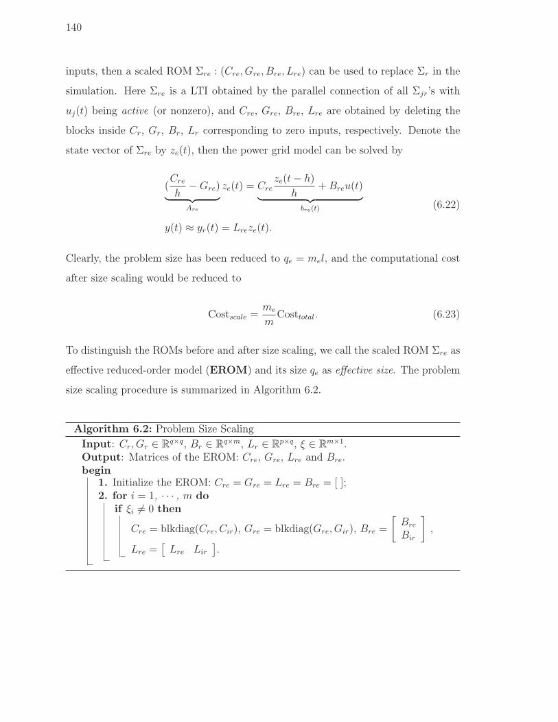
140
inputs, then a scaled ROM Σre : (Cre, Gre, Bre, Lre) can be used to replace Σr in the
simulation. Here Σre is a LTI obtained by the parallel connection of all Σjr’s with
uj(t) being active (or nonzero), and Cre, Gre, Bre, Lre are obtained by deleting the
blocks inside Cr, Gr, Br, Lr corresponding to zero inputs, respectively. Denote the
state vector of Σre by ze(t), then the power grid model can be solved by
(Cre
h−Gre)
︸ ︷︷ ︸Are
ze(t) = Creze(t− h)
h+Breu(t)
︸ ︷︷ ︸bre(t)
y(t) ≈ yr(t) = Lreze(t).
(6.22)
Clearly, the problem size has been reduced to qe = mel, and the computational cost
after size scaling would be reduced to
Costscale =me
mCosttotal. (6.23)
To distinguish the ROMs before and after size scaling, we call the scaled ROM Σre as
effective reduced-order model (EROM) and its size qe as effective size. The problem
size scaling procedure is summarized in Algorithm 6.2.
Algorithm 6.2: Problem Size Scaling
Input: Cr, Gr ∈ Rq×q, Br ∈ R
q×m, Lr ∈ Rp×q, ξ ∈ R
m×1.Output: Matrices of the EROM: Cre, Gre, Lre and Bre.begin
1. Initialize the EROM: Cre = Gre = Lre = Bre = [ ];2. for i = 1, · · · , m do
if ξi 6= 0 then
Cre = blkdiag(Cre, Cir), Gre = blkdiag(Gre, Gir), Bre =
[Bre
Bir
],
Lre =[Lre Lir
].

141
6.4.3 Parallel Computation
Equation (6.20) shows that yir(t) only depends on Lir, Air and bir(t). On a multi-
core platform, ROMs of the splitted systems can be clustered into several groups, and
then each group can be simulated simultaneously. Provided the m splitted ROMs are
clustered into N groups (N ≤ m), the simulation cost would be reduced to
Costparallel = Nb
(O(l3) +Nt ×O(l2)
)
with Nb =
m
N, if
m
N=[mN
]
([mN
]+ 1), otherwise.
(6.24)
Here, Nb is the maximum block number in each group, and [o] represents the integral
part of o. In the extremal case, an m× speedup can be achieved if each Σir is regarded
as an individual group (when N = m).
Simulation of Σre (the EROM) can be tackled in a similar way. Keeping N
unchanged and replacing m with me in (6.24), a new maximum block number Nbe
will be obtained which is normally smaller than Nbe. Therefore, the two acceleration
schemes can be used together to achieve the fastest computation if the active port
number is very large.
6.5 Discussions of BDSM
6.5.1 Comparison with Existing Power Grid MORs
Table 6.1 has compared BDSMwith some typical massive-port MOR schemes: EKS [100],
PRIMA [22], and SVDMOR [102] (a typical MOR based on terminal reduction). In
PRIMA and BDSM, we assume that l moments of the transfer matrix are matched;
in SVDMOR, we assume that the port compression ratio is α (i.e., the ratio of port

142
MOR ROM ROM Matched ROM ROMmethod size pattern moments reusable? scalable?
BDSM ml block-diagonal l yes yesPRIMA ml full dense l yes no
SVDMOR αml full dense N/A yes noEKS l full dense N/A no no
Table 6.1: Comparison of various multi-port MOR schemes. In SVDMOR, α repre-sents the port compression ratio.
number after terminal reduction w.r.t the original port number), and then l mo-
ments of the “thin” transfer matrix is matched; in EKS, it is assumed that the first
l moments of the response under a predefined excitation are captured. In SVDMOR
and EKS, the “true” moments of H(s) are not captured, so they are not exact mo-
ment matching schemes. Among these approaches, PRIMA and SVDMOR generate
full dense matrices, which are expensive for subsequent frequency/time-domain sim-
ulation. Although SVDMOR could compress the port size to some extent (at the
cost of accuracy sacrifice), the obtained dense-matrix ROMs are still memory- and
time-consuming for many-terminal systems. And when the input-output correlation
is not strong, large errors may be induced by the terminal reduction process. EKS
is capable of generating very small (size-l) macromodels, but the resulting ROMs
are not reusable. These problems lead to remarkable efficiency degradation in ROM-
based simulation. Compared with these existing MORs, BDSM does not have these
limitations, thereby allowing for more efficient simulation of massive-port networks.
We remark that EKS ROM is very inaccurate under varying input patterns, due to
its strong dependency on the predefined input waveforms. To increase its accuracy,
more moments of the response should be captured. However, as will be shown in
Section 6.6, EKS is not comparable with PRIMA and BDSM in terms of accuracy,
even if the ROM size is increased to ml, at a cost similar to that of PRIMA which
would be inefficient for power grid networks.

143
6.5.2 A Variant: Row-by-Row BDSM Scheme
If the input port number is larger than the output port number (i.e., p < m), a variant
of BDSM based on row-by-row moment matching could be developed to generate a
smaller ROM. First, the output position matrix L could be splitted as
L =
p∑
i=1
Li, with Li ∈ Rp×n, Li(j, :) =
li, if i = j
0, if i 6= j(6.25)
for i, j = 1, 2, · · · , p. Here li denotes the i-th row of L. Then the splitted LTI
system Σi can be realized by (C,G,B, Li), and the transfer matrix is written as
Hi(s) = Li(sC −G)B, and the original transfer matrix can be expressed as
H(s) =
p∑
i=1
Hi(s). (6.26)
For Σi, a projection matrix can be constructed by
V (i) = Kl(s0C −G)−TCT , (s0C −G)−TLTi (6.27)
which is an n × l matrix since Li only contains one nonzero row vector. After that,
Σir can be generated by the approach in (6.11). And finally, by parallel connection of
all Σir’s, a size pl × pl block-diagonal structured ROM could be constructed for the
original power grid model. This model contains p diagonal blocks with each block
being size-l.
It can be proved that Σir’s transfer matrix captures the i-th rows of H(s)’s first
l moment matrices. Therefore, this MOR is in fact a row-by-row moment matching.
Due to the special matrix structure, the resulting ROM can also be simulated in a
parallel style. However, using row-by-row moment matching, the problem size can
not be scaled with the active input number, because the input matrix have multiple

144
nonzero columns in each block.
6.5.3 System Passivity
A passive system is one that does not generate energy internally. System passivity is
expected to be preserved when the transfer matrix is square (i.e., p = m) and repre-
sents the admittance/impedance parameters. In such a case u(t)Ty(t) is a power met-
ric, and the resulting ROM should be positive real. The proposed BDSM can not au-
tomatically guarantee system passivity, thus passivity enforcement/compensation [10]
procedures are needed if nonpassive models are produced. The main bottleneck of
passivity enforcement on Σr lies in passivity verification. To ensure that all possible
nonpassive regions are detected, Hamiltonian method [10] or generalized Hamiltonian
method (GHM, c.f. Chapters 2 & 3) should be used which, however, consume O(q3)
complexity (q is the size of Σr). Since q might be up to thousands for multi-port
models, the passivity verification and enforcement can be prohibitively expensive.
Fortunately, the block-diagonal structure of Σr can significantly facilitate the cal-
culations. For simplicity, we assume that Σr is obtained by single-point projection
thus the size of Σir is l. We further assume that Cir is nonsingular after projec-
tion (otherwise, the Weierstrass decomposition [with O(l3) complexity] or canonical
projector technique [20] could be used to convert Σir to a nonsingular system), then
Σir can be transformed to a standard state-space model Σsir: (I, G
sir, B
sir, Lir), with
Gsir = C−1
ir Gir and Bsir = C−1
ir Bir. An eigenvalue decomposition can be performed on
Gsir at a cost of O(l3)
Gsir = XiΛiX
−1i (6.28)
where Λi is a diagonal matrix whose diagonal elements contain the eigenvalues of Gsir.
Then Σir can be realized by (I, Λi, X−1i Bs
ir, LirXi), and similar to Bi, X−1i Bs
ir also
has only one nonzero vector at the i-th column. To this end, Σr can be realized as a

145
V DD
V DD
V DD
Resistor:
Inductor:
Current source:
Capacitor:
Active area:
Power grid: 0 1 0 0 Control clock:
Figure 6.3: The upper part represents a power grid with consideration of clock gating;the bottom part is the RLC model.
diagonal-structured LTI via parallel connection of all Σi’s. And finally, the passivity
test and enforcement can be largely simplified via Laguerre’s method at the cost of
only O(q2) [109].
However, we remark that, unlike interconnect macromodeling, in may cases, sys-
tem passivity is not necessarily required to be preserved in power grid reduction. First,
the input and output numbers might not be identical (e.g., in some cases y(t) = x(t)
and p m), thus H(s) is not a square matrix. Second, even though m = p, the
output variables may not be the nodal voltage (or branch current) variables corre-
sponding to the input current (or voltage) excitations, which means that physically
H(s) does not represent the admittance/impedance parameters.

146
6.6 Numerical Results
We use several multi-domain clock gating power grid benchmarks to verify the pro-
posed scheme. As shown in Fig. 6.3, the yellow rectangular represents a power grid
system, which is modeled as a large-scale linear circuit including resistance, capac-
itance and packaging inductance (cf. the bottom part of Fig. 6.3). Time-varying
current sources are used to describe the behavior of active circuit blocks. If clock
gating technique is adopted in low power design to control the behavior of transis-
tor circuit blocks, only part of the transistor networks are active (as marked by the
red areas in Fig. 6.3), whereas other blocks are disabled. The current sources from
these “dead” blocks can be regarded as zero in transient simulation [108]. The MNA
LTI models are extracted from some industrial Spice netlists. All experiments are
performed on a 2.6GHz 4-GB RAM Linux workstation.
6.6.1 MOR Efficiency and Accuracy
We begin by timing different MOR schemes using single-point moment matching on 5
RLC power grid benchmarks (ckt1-ckt5 in Table 6.2). The port numbers range from
several tens to over 1k ; and the node numbers are from 6k to 1.7M. For simplicity, all
ports are first assumed to be active and excited by unit-impulse signals in EKS [91]; in
SVDMOR, α is set around 0.6 for all examples. Specifically,H(s) is first approximated
by UTl H(s)Ur with H(s) ∈ C
p×m, p = [αp] and m = [αm] [102], and then the “thiner”
LTI H(s) is reduced by PRIMA. Since sparse LU may still introduce large amounts
of nonzero elements for some cases, this factorization is skipped in ckts3-5 to save
memory, at the cost of more simulation time.
The CPU times and resulting ROM sizes are listed in Table 6.2. With the same
number of moments matched, BDSM and PRIMA generate ROMs with the same size.
Since much fewer long-vector orthonormalizations are needed, BDSM is faster than

147
Figure 6.4: The matrix structures of ckt1’s ROMs, obtained from BDSM and PRIMA,respectively.
PRIMA, and this speedup becomes more remarkable as the problem size and port
number increase. In SVDMOR, although the terminals can be reduced to some extent,
it still needs more orthonormalization steps and thus is slower than BDSM in many-
terminal cases (cf. ckts3-4). Even more, PRIMA and SVDMOR may fail in very-
large-size many-port cases (cf. ckts4-5). This is because: 1) the resulting full-dense
ROMs of PRIMA and SVDMOR can be memory-consuming in many-port cases; 2)
the “fat” projection matrix V (∈ Rn×ml or Rn×αml) is also dense and even more CPU-
consuming. While in BDSM the projection matrix V (i) for each splitted system is very
thin, and the final sparse block-diagonal ROM is cheap to store. To illustrate this,
Fig. 6.4 has compared the ROM matrix structures of ckt1, from BDSM and PRIMA,
respectively. Due to the special structure of Gr, Cr and Br, much smaller EROMs
can be extracted from BDSM ROMs if only a small portion of ports are active (cf.
column 4 of Table 6.2) under clock gating, which can be very efficient in subsequent
simulation. EKS is the fastest one among these schemes. However, the EKS ROM
need to be rebuilt each time when the input pattern changes, making the simulation

148
ckt nodeport number PRIMA [22] SVDMOR [102] EKS [100] BDSM No. of
total active Time Size Time Size Time Size TimeSize matched
ROM EROM moments
ckt1 6k 51 6 29.37 306 35.60 180 0.30 6 8.18 306 36 6ckt2 20k 108 19 5.0× 10³ 1080 1.4× 10³ 640 15.4 10 3.7× 10³ 1080 190 10ckt3 80k 204 21 1.2× 10⁴ 2040 1.0× 10⁴ 1220 17.7 10 7.1× 10³ 2040 210 10ckt4 123k 315 46 break down N/A break down N/A 39.8 8 2.6× 10⁴ 2520 368 8ckt5 1.7M 1429 103 break down N/A break down N/A 610 10 5.9× 10⁴ 14290 1030 10
Table 6.2: CPU times (sec) of various MOR schemes. In SVDMOR, we match themoments of the approximated low-rank transfer matrix after terminal reduction. InEKS, the moments of the response under unit impulse excitations are captured, butthe transfer matrix’s moments can not be captured, therefore, the EKS ROM is notreusable.
very inefficient in practice. Furthermore, it is also difficult to exactly predict the
input signals of a power grid network, whereas inexactly modeled inputs may make
the EKS ROM unreliable. Therefore, a reusable ROM is preferred for repeated circuit
simulation. As shown by Table 6.2, BDSM provides the best numerical efficiency
among those reusable power grid MOR schemes.
105
1010
1015
0
0.1
0.2
0.3
0.4
0.5
0.6
0.7
0.8(a) Frequency response, port (1,2)
Frequency (rad/sec)
Mag
nitu
de
105
1010
1015
10−20
10−15
10−10
10−5
100
105
(b) Relative error
Frequency (rad/sec)
Rel
ativ
e er
ror
originalBDSMPRIMASVDMOREKS, order−6EKS, order−306
BDSMPRIMASVDMOREKS, order−6EKS,order−306
Figure 6.5: Comparison of MOR accuracy for ckt1.
Fig. 6.5 plots the transfer function of port(1,2) for ckt1. In EKS, all inputs are set

149
cktstime PRIMA [22] SVDMOR [102] EKS [100] BDSM No. of No. of
withoutstime size stime size stime size
without scaling with scaling expansion matchedMORs stime size stime size points moments
ckt1 320 266 1020 44.3 600 0.20 20 12.1 1020 1.31 120 5 20ckt2 529 2.3× 10³ 3240 331 1920 0.50 30 43.2 3240 6.20 570 6 30ckt3 2.5× 10³ 1.8× 10³ 3060 259 1830 0.05 15 23.7 3060 2.44 315 5 15ckt4 5.1× 10³ N/A N/A N/A N/A 0.20 15 61.9 4725 8.84 690 5 15ckt5 5.9× 10⁴ N/A N/A N/A N/A 0.21 18 291 25722 21.7 1854 6 18
Table 6.3: CPU times (sec) of 1000-point backward Euler time-domain simulation viaROMs obtained by multi-point projection.
as unit impulse signals. For fairness, 6 moments are matched in all MOR schemes.
EKS’s size-6 ROM has very low accuracy. Then we construct a larger EKS ROM by
matching 306 moments of the response, which costs 36sec for ckt1. However, the size-
306 EKS ROM is still very inaccurate. This is not surprising, because the EKS ROM
under a specific excitation is not reusable for new input patterns. Fig. 6.5 plots the
relative errors of these MOR schemes. PRIMA and BDSM has very high accuracy
(relative error < 10−6 for ω < 1010rad/sec), due to their exact moment matching
properties. The error of SVDMOR ROM is several orders larger over those of BDSM
and PRIMA, due to the error-prone terminal reduction.
6.6.2 Time-Domain Performance
We continue to compare the behaviors of different ROMs in time-domain transient
simulation. Since practical signals are usually distributed in wide frequency bands,
rational Krylov-subspace [106] projection is employed to improve numerical accuracy.
In all MORs, l moments are matched at each expansion point, so totally ltot = lk
moments would be matched if k points are used. For simplicity, pulse waveforms
are added to all active ports as excitations. The CPU times of 1000-step transient
simulation (denoted by “stime”) are listed in Table 6.3. Because PRIMA and
SVDMOR generate large dense matrices, the numerical efficiency of their ROMs
degrades remarkably in large multi-port systems, and solving the dense ROMs can

150
0 0.2 0.4 0.6 0.8 1 1.2
x 10−7
0
0.5
1
1.5
2
2.5
3
3.5
4
4.5x 10
−3 (a)
Time (s)
Vol
tage
of n
ode−
37 (
Vol
t)
0 0.2 0.4 0.6 0.8 1 1.2
x 10−7
10−14
10−12
10−10
10−8
10−6
10−4
10−2
(b)
Time (s)
Err
or
original
BDSM ROM&EROM
PRIMA
SVDMOR
EKS, order−15
EKS, order−3060
BDSM ROM&EROM
PRIMA
SVDMOR
EKS, order−15
EKS,order−3060
Figure 6.6: The voltage waveforms of node-37 in ckt3.
be even more expensive than simulating the original networks (as shown by ckt2).
Thanks to the sparse block-diagonal structure, BDSM ROMs can be simulated very
fast even when the ROM size reaches above 20k for many-terminal models (cf. ckt5).
Furthermore, with consideration of clock gating, EROM could further speedup the
time-domain simulation (which is around 10× in our tested cases). Although EKS is
very fast in the subsequent simulation, EKS ROMs need to be rebuilt for repeated
simulation. On the other hand, EKS is not comparable to other MOR schemes in
terms of accuracy. To show this, Fig. 6.6 plots the voltage waveforms at 37th node of
ckt3, where 5 expansion points are utilized in all projection schemes. Clearly, EKS
ROM’s waveform could not capture the behavior of ckt3 with acceptable accuracy
(even when the ROM size is increased to 3060, whose simulation cost is about 2 ×10³sec). The waveforms from ROMs of BDSM, PRIMA and SVDMOR are close
to the original one. Among them, the result from BDSM can not be distinguished
from the original one, and the error is below 10−5. The parallel acceleration is not
implemented here, as its speedup factor has been analytically derived.

151
6.7 Summary
This chapter has proposed a novel model reduction scheme, BDSM, for multi-port
systems such as power grid networks. BDSM has similar accuracy to PRIMA due to
the same number of matched moments; it is faster and more memory-efficient over
PRIMA (and SVDMOR in many-terminal cases) in model generation, since lots of
long-vector orthonormalizations are skipped; unlike EKS and TBS, because BDSM
is input-independent, the obtained ROMs are reusable for time/frequency-domain
analysis under varying input patterns; more importantly, BDSM ROMs have block-
diagonal structures which in turn allow for very fast subsequent simulation. Some
acceleration techniques in the subsequent simulation, including problem size scaling
and parallel computation, have also been presented. Additional issues such as row-by-
row moment matching and passivity issue are discussed. The efficiency and accuracy
of BDSM in both model extraction as well as subsequent time-domain simulation
have been verified by industrial benchmarks.

Chapter 7
Thesis Conclusion
This thesis is centered on some theoretical and numerical problems on linear time-
invariant descriptor systems (LTI DSs), with emphasis on their passivity assessment
and model order reduction (MOR). We focus on the LTI cases, rather than linear
time-variant (LTV) or nonlinear cases, because: 1) there exist many open questions
for LTI DSs; 2) as the fundamentals of LTV and nonlinear cases, the advancements
on LTI DS studies would be applied to analyze more complex circuit systems.
7.1 Part 1: DS Passivity Assessments
Specifically, in the first part (Chapters 2 to 4), we focus on the passivity assessments
of LTI DSs, including both admittance/impedance systems and scattering systems.
Works in this part include:
1. A generalized Hamiltonian method (GHM) and its half-size version (HGHM)
have been developed, including theoretical derivation and numerical realization.
The most significant advantage of GHM/HGHM passivity test is that they are
purely algebraic routines, and therefore the test results are very accurate. Not
only they can tell a LTI DS is passive or not, but they also accurately locate
152

153
the possible nonpassive regions, and thereby provide a versatile tool for DS
passivity enforcement (if necessary).
2. Based on the work of Chapter 2, we have further presented a projector-based
passivity test for large-size LTI DS models which can not be tackled by GHM.
It is the first time that we use spectral projectors, based on a novel fast con-
struction, to efficiently decompose a large DS model to its proper and improper
subsystems. After the projector-based system decomposition, the proper part
is tested by GHM based on a fast numerical implementation. The fast GHM
implementation only computes a small part of the generalized eigenvalues that
are close to the imaginary axis, using a multi-shift Arnoldi algorithms. Since
this method is based on Krylov iteration, the algorithm is CPU-friendly and is
applicable to very large circuit models.
3. We notice that in high-frequency applications, S-parameters are more frequently
used. Motivated by this, Chapter 4 has developed the S-parameter generalized
Hamiltonian method (S-GHM) and its half-size algorithm (S-HGHM). Similar
to GHM and HGHM, S-GHM and S-HGHM can locate all possible nonpassive
regions with high numerical accuracy. Furthermore, we have also proposed a
passivity test flow for admittance/impedance DSs, based on S-GHM and S-
HGHM. It is realized by two steps. First, the admittance/impedance model
is converted to a “scattering” DS via Moebious transform. After that, the
Moebious-transformed system is tested by S-GHM or S-HGHM to find the pos-
sible nonpassive frequency intervals.
An interesting observation about the (S-parameter) generalized Hamiltonian meth-
ods is that, they are the superset of standard Hamiltonian methods and therefore

154
applicable to either DS or standard state-space models. Besides that, based on equiv-
alent model conversion, they can be applied to more general DSs or standard state-
space LTI models, without restrictions on system matrices as required by traditional
approaches.
7.2 Part 2: DS Model-Order Reduction
The second part of this thesis aims to solve two issues about DS MOR:
1. Passivity and improper part preserving MOR;
2. Efficient MOR for multi-port LTI DSs that allows for fast subsequent circuit
simulation.
Chapter 5 focuses on the first issue. The improper part of a DS is preserved
by additive system decomposition based on fast spectral projector technique. After
additive decomposition, the improper part remains unchanged, and the proper part is
reduced via DS-format positive-real balanced truncation (DS-PRBT). Since the main
bottleneck of DS-PRBT is in solving the dual generalized algebraic Riccati equations
(GAREs), we have developed a generalized quadratic alternate implicit (GQADI)
algorithm to efficiently compute the positive-real Gramians. The proposed GARE
solver is faster than the most advanced solver (e.g., Newton’s iteration based on
LR-ADI). Detailed algorithmic description, including convergence and well posedness
have been presented. To further speed up the matrix solver, a low-rank version (LR-
GQADI) has also been devised, which reduces the complexity from O(n3) to O(n2).
Finally, we aimed to construct “good” macromodels for multi-port LTI DS, such
as power grid models. Due to the large number of ports, existing MOR techniques
are not efficient for power grids. Some fast algorithms have been developed at the
expense of model accuracy. To overcome this problem, we have developed a MOR

155
routine based on input matrix splitting, called BDSM. The BDSM ROM is as accurate
as standard Krylov-subspace based moment-matching MORs; its resulting ROMs are
block-diagonal structured, and thereby are cheap to solve and easy to compute in a
parallel fashion; a very interesting result about BDSM is that, when used in power
grid simulation, the ROM size can be further significantly scaled down if power gating
is considered; finally and most importantly, the resulting ROM is reusable, so it could
be used under various input wave patterns.

Bibliography
[1] E. L. Yip and R. F. Sincovec, “Solvability, controllability and observability of con-
tinuous descriptor systems,” IEEE Trans. Automat. Control, vol. AC-26, no. 3,
pp. 702–707, 1981.
[2] L. Dai, Singular Control Systems, ser. Lecture Notes in Control and Information
Sciences 118. Berlin/Heidelberg: Springer-Verlag, 1989.
[3] A. Varga, “A descriptor systems toolbox for MATLAB,” in Proc. IEEE Intl.
Symp. Computer-Aided Control System Design, 2000, pp. 150–155.
[4] K. Zhou, J. C. Doyle, and K. Golver, Robust and Optimal Control. Upper
Sadder River, NJ: Prentice-Hall, 1996.
[5] D. E. Schwarz and C. Tischendorf, “Structural analysis of electric circuits and
consequences for MNA,” Intl. J. Circuit Theory Appl., vol. 28, pp. 131–162, 2000.
[6] D. Ioan and G. Ciuprina, “Reduced order models of on-chip passive components
and interconnects, workbench and test structures,” in Model Order Reduction:
Theory, Research Aspects and Applications. Springer, Berlin Heidelberg, Aug
2008, pp. 447–467.
156

157
[7] B. Bond and L. Daniel, “Stable Reduced Models of Nonlinear Descriptor Systems
through Piecewise Linear Approximation and Projection,” IEEE Trans. CAD of
Integrated Circuits and Systems, vol. 28, no. 10, pp. 1467–1480, 2009.
[8] S. Grivet-Talocia, “An adaptive sampling technique for passivity characterization
and enforcement of large interconnect macromodels,” IEEE Trans. Advanced
Packaging, vol. 31, no. 4, pp. 673–683, Nov 2008.
[9] D. Saraswat, R. Achar, and M. Nakhla, “Fast passivity verification and enforce-
ment via reciprocal systems for interconnects with large order macromodels,”
IEEE Trans. VLSI Syst., vol. 15, no. 1, pp. 48–59, Jan 2007.
[10] S. Grivet-Talocia, “Passivity enforcement via perturbation of Hamiltonian ma-
trices,” IEEE Trans. Circuits Syst. I, vol. 51, no. 9, pp. 1755–1769, Sept 2004.
[11] S. Grivet-Talocia and A. Ubolli, “A comparative study of passivity enforce-
ment schemes for linear lumped macomodels,” IEEE Trans. Advanced Packaging,
vol. 31, no. 4, pp. 673–683, Nov 2008.
[12] D. Saraswat, R. Achar, and M. Nakhla, “Global passivity enforcement algorithms
for macromodels of interconnect subnetworks characterized by tabulated data,”
IEEE Trans. VLSI Syst., vol. 13, no. 7, pp. 819–831, Jul 2005.
[13] B. Gustavsen and A. Semlyen, “Fast passivity assessment for S-parameter ra-
tional models via half-size test matrix,” IEEE Trans. Microwave Theory and
Technology, vol. 56, no. 12, pp. 2701–2708, Dec 2008.
[14] A. Semlyen and B. Gustavsen, “A half-size singularity test matrix for fast and
reliable passivity assessment of rational models,” IEEE Trans. Power Delivery,
vol. 24, no. 1, pp. 345–351, Jan 2009.

158
[15] E. Griepentrog and R. Marz, “Basic properties of some differential-algebraic
equations,” Zeitschrift fur Analysis und ihre Anwendungen, vol. 8, no. 1, pp.
25–40, 1989.
[16] T. Reis and T. Stykel, “Positive real and bounded real balancing
for model reduction of descriptor systems,” Institut fur Mathematik,
Technische Universitat Berlin, Tech. Rep. 2008/25, 2008. [Online]. Available:
http://www.math.tu-berlin.de/∼stykel/Publications/pr 08 25.pdf
[17] T. Reis and T. Stykel, “Passivity-preserving model reduction of differential-
algebraic equations in circuit simulation,” in Proc. Appl. Math. Mechanics.
Zurich, Switzerland, Jul 2007, pp. 1 021 601–1 021 602.
[18] T. Stykel, “Balancing-related model reduction of circuit equations using
their toplogical structure,” May 2009, available at http://www.math.tu-
berlin.de/∼stykel/.
[19] R. Marz, “Canonical projectors for linear differential algebraic equations,” Com-
puters Math. Applications, vol. 31, no. 4, pp. 121–135, Feb. 1995.
[20] N. Wong, “An efficient passivity test for descriptor systems via canonical projec-
tor techniques,” in Proc. Design Automation Conference. San Fransisco, CA,
Jul 2009.
[21] B. Brogliato, R. Lozano, B. Maschke and O. Egeland, Dissipative Systems Anal-
ysis and Control: Theory and Applications, 2nd ed., Springer, 2007.
[22] A. Odabasioglu, M. Celik, and L. Pileggi, “PRIMA: passive and reduced-order
interconnect macromodeling algorithm,” IEEE Trans. CAD of Integrated Cir-
cuits and Systems, vol. 17, no. 8, pp. 645–654, Aug 1998.

159
[23] Y. Hao, Y. Shi, and L. He, “Fast analysis of structured power grid by trian-
gularization based structure preserving model oder reduction,” in Proc. Design
Automation Conf., July 2006, pp. 205–210.
[24] Y. M. Lee, Y. Cao, T.-H. Chen, J. Wang, and C. C. Chen, “HiPRIME: hier-
archical and passivity preserved interconnect macromodeling engine for RLKC
power delivery,” IEEE Trans. CAD of Integrated Circuits and Systems, vol. 24,
no. 6, pp. 797 – 806, Jun. 2005.
[25] P. Feldmann and R. W. Freund, “Reduced-order modeling of large linear subcir-
cuits via a block Lanczos algorithms,” in Proc. Design Automation Conf., 1995,
pp. 474–479.
[26] J. R. Phillips, L. Daniel, and L. M. Silveira, “Guaranteed passive balancing
transformations for model order reduction,” IEEE Trans. CAD of Integrated
Circuits and Systems, vol. 22, no. 8, pp. 1–15, Aug 2003.
[27] L. M. Silveira and J. R. Phillips, “Resampling plans for sample point selection
in multipoint model-order reduction,” IEEE Trans. CAD of Integrated Circuits
and Systems, vol. 25, no. 12, pp. 2775 – 2783, Dec 2006.
[28] J. R. Phillips and L. M. Silveira, “Poor man’s TBR: a simple model reduction
scheme,” IEEE Trans. CAD of Integrated Circuits and Systems, vol. 24, no. 1,
pp. 43 – 55, Jan 2005.
[29] G. Muscato, G. Nunnari, and L. Fortuna, “Singular perturbation approximation
of bounded real and of positive real transfer matrices,” in American Control
Conf., June-1 July 1994, pp. 3416–3420.

160
[30] N. Wong and V. Balakrishnan, “Fast positive-real balanced truncation via
quadratic alternating direction implicit iteration,” IEEE Trans. CAD of Inte-
grated Circuits and Systems, vol. 26, no. 9, pp. 1725–1731, Sept 2007.
[31] B. N. Bond and L. Daniel, “A piecewise-linear moment-matching approach to
parameterized model-order reduction for highly nonlinear systems,” IEEE Trans.
CAD of Integrated Circuits and Systems, vol. 26, no. 12, pp. 2116 – 2129, Dec
2007.
[32] P. Li and L. Pileggi, “Compact reduced-order modeling of weakly nonlinear ana-
log and RF circuits,” IEEE Trans. CAD of Integrated Circuits and Systems,
vol. 24, no. 2, pp. 184–203, Feb 2005.
[33] N. Dong and J. Roychowdhury, “General-purpose nonlinear model order reduc-
tion based on piecewise polynomial representations,” IEEE Trans. CAD of In-
tegrated Circuits and Systems, vol. 27, no. 2, pp. 249–261, Feb 2008.
[34] L. Daniel, C. S. Ong, S. C. Low, K. H. Lee, and J. White, “A multiparameter
moment matching model reduction approach for generating geometrically pa-
rameterized interconnect performance models,” IEEE Trans. CAD of Integrated
Circuits and Systems, vol. 23, no. 5, pp. 678–693, May 2004.
[35] N. Mi, S. X.-D. Tan, Y. Cai, and X. Hong, “Fast variational analysis of on-chip
power grids by stochastic extended Krylov subspace method,” IEEE Trans. CAD
of Integrated Circuits and Systems, vol. 27, no. 11, pp. 1996–2006,
[36] Y. Liu, L. Pileggi and A. J. Strojwas, “Model order-reduction of RC(L) inter-
connect including variational analysis,” in Proc. Design Automation Conference,
vol. 27, no. 11, pp. 1996–2006, June 1999

161
[37] M. Pedram and S. Nazarian, “Thermal modeling, analysis and management in
VLSI circuits: principles and methods,” Proc. of IEEE, Special Issue on Thermal
Analysis of ULSI, Vol. 94, No. 8, pp. 1487–1501, Aug. 2006.
[38] A. H. Ajami, K. Banerjee, and M. Pedram, “Modeling and analysis of non-
uniform substrate temperature effects in high performance VLSI,” IEEE Trans.
CAD of Integrated Circuits and Systems, Vol. 24, No. 6, pp. 849-861, Jun. 2005.
[39] R. W. Freund, “An extension of positive real lemma to descriptor systems,”
Optimization Methods and Software, vol. 19, no. 1, pp. 69–87, Feb 2004.
[40] G. H. Golub and C. F. V. Loan, Matrix Computations, 3rd ed. Johns Hopkins
University Press, Baltimore, MD, 1996.
[41] Y. Liu and N. Wong, “Fast sweeping methods for checking passivity of descriptor
systems,” in Proc. IEEE Asia Pacific Conf. on Circuits and Systems, Dec. 2008,
pp. 1794–1797.
[42] D. Chu and R. C. E. Tan, “Algebraic characterizations for positive realness of
descriptor systems,” SIAM J. Matrix Anal. Appl., vol. 30, no. 1, pp. 197–222,
2008.
[43] C. Yang, Q. Zhang, Y. Lin, and L. Zhou, “Positive realness and absolute stability
problem of descriptor systems,” IEEE Trans. Circuits Syst. I, vol. 54, no. 5, pp.
1142–1149, May 2007.
[44] L. Zhang, J. Lam, and S. Xu, “On positive realness of descriptor systems,” IEEE
Trans. Circuits and Syst. I, vol. 49, no. 3, pp. 401–407, Mar. 2002.
[45] H. S. Wang, C. F. Yung, and F. R. Chang, “Bounded real lemma and H∞
control for descriptor systems,” IEE Proc. Control Theory Appl., vol. 145, no. 3,
pp. 316–322, 1998.

162
[46] N. Wong and C. Chu, “A fast passivity test for stable descriptor systems via
skew-Hamiltonian/ Hamiltonian matrix pencil transformations,” IEEE Trans.
Circuits and Syst. I, vol. 55, no. 2, pp. 635–643, Mar 2008.
[47] P. Benner and D. Chu, “A new test for passivity of descriptor systems,” Ober-
wolfach reports, Mathematisches Forschungsinstitut Oberwolfach, Tech. Rep.
11/2005, Feb. 2005.
[48] B. Gustavsen and A. Semlyen, “Rational approximation of frequency domain
responses by vector fitting,” IEEE Trans. Power Delivery, vol. 14, no. 3, pp.
1052–1061, July 1999.
[49] A. Mayo and A. Antoulas, “A framework for the solution of the generalized
realization problem,” Linear Algebra Appl., vol. 425, no. 2–3, pp. 634–662, Sep.
2007.
[50] S. Lefteriu and A. C. Antoulas, “Modeling multi-port systems from frequency
response data via tangential interpolation,” in Proc. IEEE Workshop on Signal
Propagation on Interconnects, May 2009, pp. 1–4.
[51] A. C. Antoulas, D. C. Sorensen and S. Gugercin, “A survey of model reduction
methods for large-scale systems,” Contemporary Mathematics, vol. 280, pp. 193–
219, 2001.
[52] L. T. Pillage and R. A. Rohrer, “Asymptotic Waveform Evaluation for Timing
Analysis,” IEEE Trans. CAD of Integrated Circuits and Systems, pp. 352-366,
April 1990.
[53] K. J. Kerns , I. L. Wemple and A. T. Yang, “Stable and efficient reduction
of substrate model networks using congruence transforms,” in Proc. Intl. Conf.
Computer-Aided Design, pp. 207–214, Nov. 1995, San Jose, CA

163
[54] T. Stykel, “Gramian based model reduction for descriptor systems,”Mathematics
of Control, Signals, and Systems, vol. 16, no. 4, pp. 297–319, Mar 2004.
[55] ——, “Generalized alternating direction implicit method for projected general-
ized algebraic Lyapunov equations,” in Proc. Appl. Math. Mechanics, 2004, pp.
686–687.
[56] ——, “Low-rank iterative methods for projected generalized Lyapunov equa-
tions,” Electron. Trans. Numer. Anal., vol. 30, pp. 187–202, 2008.
[57] J. Li and J. White, “Reduction of large circuit models via low rank approximate
gramians”, International Journal of Applied Mathematics and Computer Science,
vol. 11, no. 5, pp. 101–121, 2001.
[58] J. Li and J. White, “Low rank solution of Lyapunov equations”, SIAM J. Matrix
Anal. Appl., vol. 24, no. 1, pp. 260–280, 2004
[59] J. M. Badia, P. Benner, R. Mayo, and E. Quintana-Orti, Parallel solution of
large-scale and sparse generalized algebraic Riccati equations. Springer Berlin,
2006.
[60] R. Byers and P. Benner, “A structure-preserving method for generalized alge-
braic Riccati equations based on pencil arithmetic,” in Proc. Euro. Control Conf.
Cambridge, UK, Sep 2003.
[61] H. Banks, R. del Rosario, and H. Tran, “Proper orthogonal decomposition-based
control of transverse beem vibrations: experimental implementations,” IEEE
Trans. Control Syst. Techonl., vol 10, no. 5, pp. 717–726, Sep. 2000.
[62] M. Rathinam and L. R. Petzold, “ A new look at proper orthogonal decomposi-
tion,” SIAM J. Numer. Anal., vol 41, no. 5, pp. 1893–1925, 2003.

164
[63] H. Heeb and A. Ruehli, “Three-dimensional interconnect analysis using partial
element equivalent circuits,” IEEE Trans. Circuits Syst. I, vol. 39, no. 11, pp.
974–982, Nov 1993.
[64] Z. Bai and R. Freund, “Eigenvalue-based characterization and test for positive
realness of scalar transfer functions,” IEEE Trans. Autom. Contr., vol. 45, no. 12,
pp. 2396–2402, Dec 2000.
[65] Z. Zhang, C. U. Lei, and N. Wong, “GHM: a generalized Hamiltonian method
for passivity test of impedance/admittance descriptor systems,” in Proc. Intl.
Conf. Computer Aided Design. San Jose, CA, Nov 2009.
[66] R. Ionutiu, J. Rommes, and A. Antoulas, “Passivity-preserving model reduction
using dominant spectral-zero interpolation,” IEEE Trans. CAD of Integrated
Circuits and Systems, vol. 27, no. 12, pp. 2250–2263, Dec 2008.
[67] K. E. Brenan, S. L. Campbell, and L. Petzold, Numerical Solution of Initial-Value
Problems in Differential Algebraic Equations, 2nd ed., ser. Classics in Applied
Mathematics. Philadelphia, PA: SIAM, 1996, vol. 14.
[68] E. Eich-Soellner and C. Fuhrer, Numerical Methods in Multibody Dynamics.
Stuttgart, Germany: B. G. Teubner, Jul. 1998.
[69] M. Gunther and U. Feldmann, “CAD-based electric-circuit modeling in industry
I: Mathematical structure and index of network equations. II Impact of circuit
configurations and parameters.” Surveys Math. Indust., vol. 8, no. 2, pp. 97–129,
131–157, 1999.
[70] I. Balk, “On a passivity of the Arnoldi based model order reduction for full-
wave electromagnetic modeling,” IEEE Trans. Adv. Packag., vol. 24, no. 3, pp.
304–308, Aug. 2001.

165
[71] B. Yan, S.-D. Tan, and B. McGaughy, “Second-order balanced truncation for
passive-order reduction of RLCK circuits,” IEEE Trans. Circuits Syst. II, vol. 55,
no. 9, pp. 942–946, Sep. 2008.
[72] R.-C. Li, “Test positive realness of a general transfer function matrix,”
Department of Mathematics, University of Kentucky, Tech. Rep. 2000-20, 2004.
[Online]. Available: http://www.ms.uky.edu/∼math/MAreport/00-20.ps
[73] E. Griepentrog and R. Marz, “Basic properties of some differential-algebraic
equations,” Zeitschrift fur Analysis und ihre Anwendungen, vol. 8, no. 1, pp.
25–40, 1989.
[74] R. Marz, “Projectors for matrix pencils,” Humboldt-Universitat zu Berlin,
Tech. Rep. 04-24, 2004. [Online]. Available: http://www.mathematik.hu-
berlin.de/publ/pre/2004/P-04-24.ps
[75] W. Cauer, Synthesis of Linear Communication Networks. New York: McGraw-
Hill, 1958.
[76] Z. Zhang and N. Wong, “Passivity test of immitance descriptor systems based on
generalized Hamiltonian methods,” IEEE Trans. Circuits Syst. II, vol. 57, no. 1,
pp. 61–65, Jan. 2010.
[77] T. Reis and T. Stykel, “Passivity-preserving balanced truncation for elec-
trical circuits,” Institut fur Mathematik, Technische Universitat Berlin,
Tech. Rep. 2008/32, 2008. [Online]. Available: http://www.math.tu-
berlin.de/∼stykel/Publications/pr 08 32.pdf
[78] S. Grivet-Talocia and A. Ubolli, “On the generation of large passive macromodels
for complex interconnect structures,” IEEE Trans. Advanced Packaging, vol. 29,
no. 1, pp. 39–54, Feb. 2006.

166
[79] P. Kowal. (2006, May) Null space of a sparse matrix. Matlab Central. [Online].
Available: http://www.mathworks.co.uk/matlabcentral/fileexchange/11120
[80] J. Demmel and B. Kagstrom, “The generalized Schur decomposition of an arbi-
trary pencil A-λB: robust software with error bounds and applications. Part I:
theory and algorithms,” ACM Trans. Math. Softw., vol. 19, no. 2, pp. 160–174,
Jun. 1993.
[81] M. Gerdin, “Computation of a canonical form for linear differential-algebraic
equations,” Department of Electrical Engineering, Link?ping University, SE-581
83 Linkoping, Sweden, Tech. Rep. LiTH-ISY-R-2602, Apr. 2004.
[82] B. Kagstrom and P. V. Dooren, “A generalized state space approach for the
additive decomposition of a transfer matrix,” Intl. J. Numer. Lin. Alg. Appl.,
vol. 1, no. 2, pp. 165–181, 1992.
[83] P. Benner, Scientific Computing in Electrical Engineering SCEE 2008, ser.
Mathematics in Industry, J. Roos and L. R. J. Costa, Eds. Berlin/Heidelberg:
Springer-Verlag, 2009, vol. 14. [Online]. Available: http://www-user.tu-
chemnitz.de/∼benner/pub/Benner SCEE2008 revised.pdf
[84] Y. Chahlaoni and P. V. Dooren, “A collection of benchmark examples
for model reduction of linear time invariant dynamical systems,” Feb.
2002, SLICOT Working Note. [Online]. Available: http://www.icm.tu-
bs.de/NICONET/benchmodred.html
[85] J. Ekman, G. Antonini, A. Orlandi, and A. E. Ruehli, “Stability of PEEC models
with respect to partial element accuracy,” in Intl Symp. Electromagnetic Com-
patibility, Aug. 2004, pp. 271–276.

167
[86] P. Benner, V. Mehrmann, V. Sima, S. Van-Huffel, and A. Varga, “SLICOT-a
subroutine library in systems and control theory,” Appl. and Comput. Control,
Signals, and Circuits, vol. 1, pp. 499–539, 1999.
[87] H. Wu and A. C. Cangellaris, “Model-order reduction of finite-element approx-
imations of passive electromagnetic devices including lumped electrical-circuit
models,” IEEE Trans. Microwave Theory and Tech., vol. 52, no. 9, pp. 2305 –
2313, Sep 2004.
[88] N. Marques, M. Kamon, L. Silveira, and J. White, “Generating compact, guar-
anteed passive reduced-order models of 3-D RLC interconnects,” IEEE Trans.
Advanced Packaging, vol. 27, no. 4, pp. 569–580, Nov 2004.
[89] Z. Zhang and N. Wong, “An extension of the generalized Hamiltonian method
to S-parameter descriptor systems,” in Proc. Asia South Pacific Design Autom.
Conf. Taipei, Jan 2010, pp. 43–47.
[90] Z. Zhang and N. Wong, “An efficient projector-based passivity test for descriptor
systems,” IEEE Trans. CAD of Integrated Circuits and Systems, accepted.
[91] Y. Hao, Y. Shi, and L. He, “Fast analysis of structured power grid by trian-
gularization based structure preserving model oder reduction,” in Proc. Design
Automation Conf., July 2006, pp. 205–210.
[92] Y. Yan, S. Tan, P. Liu and B. McGaughy, “Passive interconnect macromodeling
via balanced truncation of linear systems in descriptor form,” in Proc. Asia South
Pacific Design Automation Conf., Jan 2007, pp. 355–360
[93] Q. Zhou, K. Sun, K. Mohanram, and D. C. Sorensen, “Large power grid analysis
using domain decomposition,” in Proc. European Design and Test Conf. Munich,
Germany, J 2006, pp. 27–22.

168
[94] T. Chen and C. C. Chen, “Efficient large-scale power grid analysis based on pre-
conditioned Krylov -subspace iterative method,” in Proc. Design Autom. Conf.,
Jun 2001, pp. 559–562.
[95] H. F. Qian, S. R. Nassif, and S. S. Sapatnekar, “Random walks in a supply
network,” in Proc. Design Autom. Conf., Jun 2003, pp. 93–98.
[96] E. Chiprout, “Fast flip-chip power grid analysis via locality and grid shells,” in
Proc. IEEE Intl. Conf. Computer Aided Design, Nov 2004, pp. 485–488.
[97] J. N. Kozhaya, S. R. Nassif, and F. N. Najm, “A multi-grid like technique for
power grid analysis,” IEEE Trans. CAD of Integrated Circuits and Systems,
vol. 21, no. 10, pp. 1148–1160, Oct 2002.
[98] Z. Feng and P. Li, “Multigrid on GPU: tackling power grid analysis on parallel
SIMT platforms,” in Proc. IEEE Intl. Conf. Computer Aided Design. San Jose,
CA, Nov 2008, pp. 647–654.
[99] J. Li, F. Wang, and J. White, “An efficient Lyapunov equation-based approach
for generating reduced-order models of interconnect,” in Proc. Design Automa-
tion Conf., Aug 1999, pp. 1–6.
[100] J. M. Wang and T. V. Nguyen, “Extended Krylov subspace method for re-
duced order analysis of linear circuits with multiport sources,” in Proc. Design
Automation Conf., 2000, pp. 247–252.
[101] D. Li, S. X.-D. Tan, and B. McGaughy, “ETBR: Extended truncated balanced
realization method for on-chip power grid network analysis,” in Proc. European
Design and Test Conf., 2008, pp. 432–437.

169
[102] P. Feldman and F. Liu, “Sparse and efficient reduced order modeling of linear
subcircuits with large number of terminals,” in Proc. Intl. Conf. on Computer
Aided Design, 2004, pp. 88–92.
[103] P. Li and W. Shi, “Model order reduction of linear networks with massive ports
via frequency-dependent port packing,” in Proc. Design Automation Conf., 2006,
pp. 267–272.
[104] B. Yan, L. Zhou, S. X.-D. Tan, J. Chen, and B. McGaughy, “DeMOR: decen-
tralized model order reduction of linear networks with passive ports,” in Proc.
Design Automation Conf., 2008, pp. 409–414.
[105] S. Huda, M. Mallick, and J. H. Anderson, “Clock gating architectures for FPGA
power reduction,” in Proc. Intl. Conf. Field Programmable Logic and Appl., 2009,
pp. 112–118.
[106] I. M. Elfadel and D. L. Ling, “A block rational Arnoldi algorithm for multipoint
passive model order reduction of multiport RLC networks,” in Proc. Intl. Conf.
Computer Aided Design. San Jose, CA, Nov 1997, pp. 66–71.
[107] T. V. Nguyen and J. Li, “Multipoint Pade approximation using a rational block
Lanczos algorithm,” in Proc. Intl. Conf. Computer Aided Design. San Jose, CA,
Nov 1997, pp. 72–75.
[108] W. Zhang, W. Yu, X. Hu, L. Zhang, R. Shi, H. Peng, Z. Zhu, L. Chua-Eoan,
R. Murgai, T. Shibuya, N. Ito, and C.-K. Cheng, “Efficient power network anal-
ysis considering multidomain clock gating,” IEEE Trans. CAD of Integrated Cir-
cuits and Systems, vol. 28, no. 9, pp. 1348–1358, Sept 2009.

170
[109] Z. Ye, L. M. Silveira, and J. R. Phillips, “Fast and reliable passivity assess-
ment and enforcement with extended Hamiltonian pencil,” in Proc. Intl. Conf.
Comput.-Aided Design. San Jose, CA, Nov 2009, pp. 774–769.

Publications during M.Phil Study
Journal Articles
1. Y. Wang, Z. Zhang, C.-K. Koh, G. K.-H. Pang and N. Wong, “Passivity en-
forcement for descriptor systems via Hamiltonian matrix pencil perturbation,”
IEEE Transactions on Computer-Aided Design of Integrated Circuits and Sys-
tems, under review.
2. Z. Zhang and N. Wong, “An efficient projector-based passivity test for de-
scriptor systems,” IEEE Transactions on Computer-Aided Design of Integrated
Circuits and Systems, vol. 29, no. 8, pp. 1203-1214, Aug. 2010.
3. Z. Zhang and N. Wong, “Passivity check of S-parameter descriptor systems
via S-parameter generalized Hamiltonian methods,” IEEE Transactions on Ad-
vanced Packaging, vol., no., pp., 2010, accepted and in press.
4. N. Wong and Z. Zhang, “Discussion of “A half-size singularity test matrix for
fast and reliable passivity assessment of rational models,” IEEE Transactions
on Power Delivery, vol. 25, no. 2, pp. 1212-1213, Apr. 2010.
5. Z. Zhang and N. Wong, “Passivity test of immittance descriptor systems based
on generalized Hamiltonian methods,” IEEE Transactions on Circuits and Sys-
tems II, vol. 57, no. 1, pp. 61-65, Jan. 2010.
171

172
Conference Papers
1. Zheng Zhang, Xiang Hu, Chung-Kuan Cheng and Ngai Wong, “A block-
diagonal structured model reduction scheme for power grid networks,” in Proc.
Design, Automation and Test in Europe (DATE), submitted.
2. C. Y. Lin, Z. Zhang, N. Wong and H. K.-H. So, “Design space exploration
for sparse matrix-matrix multiplication on FPGAs,” in Proc. Intl. Conf. on
Field-Programmable Technology (FPT), Dec. 2010, to appear
3. Y. Wang, Z. Zhang, C.-K. Koh, G. K.-H. Pang and N. Wong, “PEDS: passivity
enforcement for descriptor systems via Hamiltonian-Symplectic matrix pencil
perturbation,” in Proc. Intl. Conf. Computer Aided Design (ICCAD), pp. ,
Nov. 2010, to appear
4. C. Y. Lin, Z. Zhang, N. Wong and H. K.-H. So, “Power-delay and energy-
delay tradeoffs in sparse matrix-matrix multiplication on FPGAs,” in Proc.
Intl. Workshop on Highly Efficient Accelerators and Reconfigurable Technologies
(HEART), Jun. 2010, to appear
5. Z. Zhang and N. Wong, “An extension of the generalized Hamiltonian method
to S-parameter descriptor systems,” in Proc. Asia and South Pacific Design
Automation Conference (ASP-DAC), pp. 43-47, Jan. 2010.
6. Z. Zhang, C.-U. Lei and N. Wong, “GHM: a generalized Hamiltonian method
for passivity test of impedance/admittance descriptor systems,” in Proc. Intl.
Conf. Computer Aided Design (ICCAD), pp. 767-773, Nov. 2009.