Embed Size (px)
Citation preview
PNNL-23997
Prepared for the U.S. Department of Energy
under Contract DE-AC05-76RL01830
Particle Release Experiment (PRex)
Final Report
ME Keillor BD Milbrath
LM Arrigo JP Rishel
RS Detwiler A Seifert
WJ Kernan CE Seifert
RR Kirkham JE Smart
M MacDougall D Emer1
V Chipman1
September 2014
1 National Security Technologies LLC


PNNL-23997
Particle Release Experiment (PRex)
Final Report
ME Keillor BD Milbrath
LM Arrigo JP Rishel
RS Detwiler A Seifert
WJ Kernan CE Seifert
RR Kirkham JE Smart
M MacDougall D Emer1
V Chipman1
September 2014
Prepared for
the U.S. Department of Energy
under Contract DE-AC05-76RL01830
Pacific Northwest National Laboratory
Richland, Washington 99352
1 National Security Technologies LLC
PNNL-23997
iii
Abstract
An experiment to release radioactive particles representative of small-scale venting from an underground
nuclear test was conducted to gather data in support of treaty verification and monitoring activities. For
this experiment, a CO2-driven “air cannon” was used to release 140
La at ambient temperatures.
Lanthanum-140 was chosen to represent the fission fragments because of its short half-life and prominent
gamma-ray emissions; the choice was also influenced by the successful production and use of 140
La with
low levels of radioactive contaminants in a Defence Research and Development Canada Field Trial. The
source was created through activation of high-purity natural lanthanum oxide at the reactor of Washington
State University, Pullman, Washington. Multiple varieties of witness plates and air samplers were laid in
an irregular grid covering the area over which the plume was modeled to deposit. Aerial survey, a
NaI(Tl) mobile spectrometer, and handheld and backpack instruments ranging from polyvinyl toluene to
high-purity germanium were used to survey the plume. Additionally, three varieties of soil sampling
were investigated. The relative sensitivity and utility of sampling and survey methods are discussed in
the context of On-Site Inspection. The measurements and samples show a high degree of correlation and
form a valuable set of test data.

PNNL-23997
v
Executive Summary
The Comprehensive Nuclear-Test-Ban Treaty is a nuclear non-proliferation treaty adopted by the
United Nations and open for signature and ratification or accession by States Parties, but not yet entered
into force. The CTBT makes provision for a verification regime that includes the conduct of an On-Site
Inspection. The sole purpose of an OSI is to determine whether a nuclear explosion has occurred in
violation of the Treaty and, if so, gather facts that might assist in identifying the violator. The Treaty
allows for an OSI to include many techniques, including the radionuclide techniques of gamma radiation
survey and spectrometry and environmental sampling and analysis (of solids, liquids, and gases). A good
understanding of the possible contamination distribution, along with the most valuable equipment and
search techniques for locating accessible radioactive contamination, would dramatically improve the
likelihood of conducting a successful OSI. In support of future OSIs, Pacific Northwest National
Laboratory conducted work to understand the realistic distribution of nuclides that might occur under
actual venting conditions from an underground nuclear test.
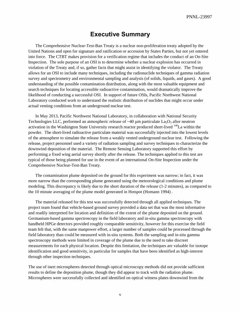
In May 2013, Pacific Northwest National Laboratory, in collaboration with National Security
Technologies LLC, performed an atmospheric release of ~40 µm particulate La2O3 after neutron
activation in the Washington State University research reactor produced short-lived 140
La within the
powder. The short-lived radioactive particulate material was successfully injected into the lowest levels
of the atmosphere to simulate the release from a weakly vented underground nuclear test. Following the
release, project personnel used a variety of radiation sampling and survey techniques to characterize the
downwind deposition of the material. The Remote Sensing Laboratory supported this effort by
performing a fixed wing aerial survey shortly after the release. The techniques applied to this test are
typical of those being planned for use in the event of an international On-Site Inspection under the
Comprehensive Nuclear-Test-Ban Treaty.
The contamination plume deposited on the ground for this experiment was narrow; in fact, it was
more narrow than the corresponding plume generated using the meteorological conditions and plume
modeling. This discrepancy is likely due to the short duration of the release (1-2 minutes), as compared to
the 10 minute averaging of the plume model generated in Hotspot (Homann 1994) .
The material released for this test was successfully detected through all applied techniques. The
project team found that vehicle-based ground survey provided a data set that was the most informative
and readily interpreted for location and definition of the extent of the plume deposited on the ground.
Germanium-based gamma spectroscopy in the field laboratory and in-situ gamma spectroscopy with
handheld HPGe detectors provided roughly comparable sensitivity, however for this exercise the field
team felt that, with the same manpower effort, a larger number of samples could be processed through the
field laboratory than could be measured with in-situ systems. Both the sampling and in-situ gamma
spectroscopy methods were limited in coverage of the plume due to the need to take discreet
measurements for each physical location. Despite this limitation, the techniques are valuable for isotope
identification and good sensitivity, in particular for samples that have been identified as high-interest
through other inspection techniques.
The use of inert microspheres detected through optical microscopy methods did not provide sufficient
results to define the deposition plume, though they did appear to track with the radiation plume.
Microspheres were successfully collected and identified on optical witness plates downwind from the

PNNL-23997
vi
release. In order to use this method with more viable results, it would be necessary to release a larger
quantity of microspheres. The use of colored or fluorescent microspheres would also aid in
discriminating the released microspheres from naturally occurring spherical particles.
PNNL-23997
vii
Acknowledgments
This work would not have been possible without the support of many people from several
organizations. The authors express their gratitude to the National Nuclear Security Administration,
Defense Nuclear Nonproliferation Research and Development, and the Comprehensive Inspection
Technologies working group, a multi-institutional and interdisciplinary group of scientists and
engineers. This work was performed by Pacific Northwest National Laboratory under award number DE-
AC52-06NA25946.


PNNL-23997
ix
Acronyms and Abbreviations
AGL Above ground level
ALARA As Low As Reasonably Achievable
ASL Above mean sea level
AMS Aerial Measuring System
ATM Atmospheric transport model(ing)
ATV All-terrain vehicle
CA Contaminated area
CFM Cubic Feet per Minute
CSS Comprehensive Sampling/Survey (Site)
CTBT(O) Comprehensive Nuclear Test-Ban-Treaty (Organization)
FL Field Laboratory
GIS Geographic Information System
GM Geiger-Mueller
GPS Global Positioning System
GZ Ground zero
HCA High Contamination Area
HDPE High Density Polyethylene
HPGe High purity germanium
ISOCS In Situ Object Counting Systems – Canberra Industries
MCNP Monte Carlo N-Particle Transport Code
MDA Minimum detectable activity
MEDA Meteorological data acquisition
NCNS National Center for Nuclear Security
NNSS Nevada National Security Site
NOAA National Oceanic and Atmospheric Administration
NSTec National Security Technologies LLC
NTS Nevada Test Site
NWS National Weather Service
OSI On-Site Inspection
PAPR Powered air-purifying respirators
PDT Pacific Daylight Time
PNNL Pacific Northwest National Laboratory
PPE Personal protective equipment
PRex Particle Release Experiment
PVC Polyvinyl chloride
PVT Polyvinyl toluene

PNNL-23997
x
RCT Radiological Control Technician
ROI Region of interest
RSI Radiation Solutions Inc.
RSL Remote Sensing Laboratory
RWP Radiological work permit
UTC Coordinated universal time
UTM Universal mean time
WSU Washington State University
PNNL-23997
xi
Contents
Abstract ....................................................................................................................................................... iii
Executive Summary .................................................................................................................................... v
Acknowledgments ..................................................................................................................................... vii
Acronyms and Abbreviations ................................................................................................................... ix
1.0 Introduction ............................................................................................................................ 1
1.1 Background .............................................................................................................................. 1
1.2 Objective .................................................................................................................................. 2
1.3 Scope of Document .................................................................................................................. 2
2.0 Experimental Considerations ................................................................................................ 3
2.1 Overview of PRex .................................................................................................................... 3
2.2 Constraints ............................................................................................................................... 3
2.3 Assumptions ............................................................................................................................. 4
2.4 Pre-Execution Release Parameters ........................................................................................... 4
3.0 PRex Experiment Preparation .............................................................................................. 6
3.1 Experiment Plan ....................................................................................................................... 6
3.2 Site Selection............................................................................................................................ 6
3.3 Background Measurements, September and October 2012 ..................................................... 7
3.4 Source Production .................................................................................................................... 9 3.4.1 Preparation of La2O3 Powder .................................................................................................................. 9 3.4.2 Irradiation at Washington State University ........................................................................................... 12 3.4.3 Source Transport ................................................................................................................................... 14
3.5 Release Mechanism ................................................................................................................ 19
3.6 Meteorology Planning and Modeling ..................................................................................... 22
3.7 NNSS Experiment Site Preparation ....................................................................................... 22 3.7.1 Posting Contamination and High Contamination Areas ....................................................................... 22 3.7.2 Prepositioned Sampling ........................................................................................................................ 22
4.0 PRex Experiment Execution ............................................................................................... 28
4.1 Time and Location ................................................................................................................. 28
4.2 Meteorological Conditions during Release ............................................................................ 28
4.3 Sampling Network ................................................................................................................. 32 4.3.1 Collection of Witness Plates ................................................................................................................. 32 4.3.2 Soil Sampling ....................................................................................................................................... 33 4.3.3 Air Sampling ......................................................................................................................................... 36
4.4 Radiation Survey .................................................................................................................... 36 4.4.1 Vehicle Survey...................................................................................................................................... 37 4.4.2 Handheld/Man-portable ........................................................................................................................ 38 4.4.3 Aerial Survey ........................................................................................................................................ 39
4.5 Field Laboratory ..................................................................................................................... 40

PNNL-23997
xii
5.0 Analysis of Results ............................................................................................................... 44
5.2 Witness Plate Laboratory Measurement Results .................................................................... 52
5.3 Comparison of Vehicle Survey and Witness Plate Results .................................................... 54
5.4 Variability at Comprehensive Sampling Sites ....................................................................... 55
5.5 Airborne Survey ..................................................................................................................... 56
5.6 Results from Soil Sampling Methods .................................................................................... 58
5.7 In-Situ Measurements ............................................................................................................ 59
5.8 Comparison of Plume Modeling to Radiometric Results....................................................... 62
5.9 Optical Witness Plate Results ................................................................................................ 65
5.10 Air Sampling Results ............................................................................................................. 71
6.0 Lessons Learned ................................................................................................................... 75
6.1 Lessons Learned ..................................................................................................................... 75 6.1.1 OSI-Relevant Lessons Learned ............................................................................................................ 75 6.1.2 Experiment-Specific Lessons Learned ................................................................................................. 77
7.0 Conclusions and Recommendations ................................................................................... 79
7.1 Recommended Future Work .................................................................................................. 80
8.0 References ............................................................................................................................. 81
Appendix A Ground Vehicle Survey Data Corrections....................................................................... A.1
Appendix B Field Laboratory Gamma Assay Results ......................................................................... B.1
Appendix C Sequence of Events / Events Log ...................................................................................... C.1

PNNL-23997
xiii
Figures
Figure 2.1: PRex test location on the Nevada National Security Site ............................................... 5
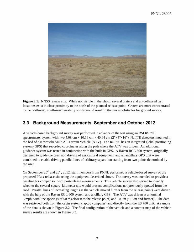
Figure 3.1: NNSS release site. While not visible in the photo, several craters and un-collapsed
test locations exist in close proximity to the north of the planned release point. Craters are
more concentrated to the northwest; south-southwesterly winds would result in the fewest
obstacles for ground survey. ....................................................................................................... 7
Figure 3.2: Screen capture made with the RSI Software RadAssist and a GIS module showing
raw data from the September 2011 background survey .............................................................. 8
Figure 3.3: ATV used for vehicle survey at the PRex location on Yucca Flats (left); contour map
of radiation survey results (right) ................................................................................................ 8
Figure 3.4: Gross count exposure map measured over the PRex release area in October 2012 ....... 9
Figure 3.5: Shaker / sieve setup including shaker, sieves, balance, and sample jars in a nitrogen
filled glove bag ......................................................................................................................... 10
Figure 3.6: Shaker and sieves are shown on the left. The sieve cover with La2O3 powder is
shown on the right. .................................................................................................................... 10
Figure 3.7: The roll-sealed aluminum can provided by the WSU Reactor Center team. This can
has been certified by the reactor center for use with non-dispersible materials. PNNL
leveraged the “certified” status of this geometry as well as the geometry specific insertion
and retrieval equipment already in place at the reactor center. ................................................. 12
Figure 3.8: The 6061-T6 aluminum liner assembly. Light blue section includes a thin septum
end with appropriate reinforcement areas to reduce stress. Green section is the welded end
cap with a 1/2" 20-threaded plug. The light purple area is a high density polyethylene plug
gasket. ....................................................................................................................................... 13
Figure 3.9: A 20-foot drop test conducted with a water-filled aluminum “can liner” resulted in
the expected amount of deformation, with no rupture or leakage............................................. 13
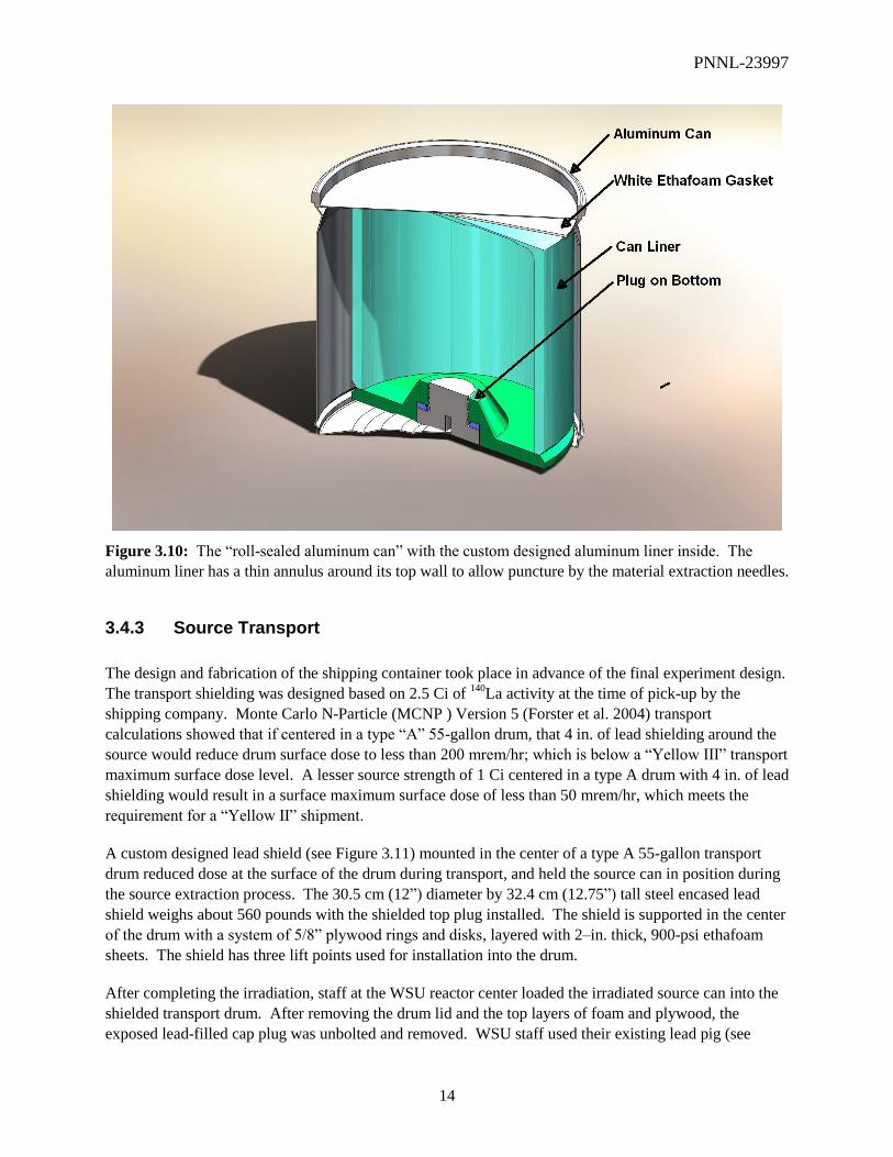
Figure 3.10: The “roll-sealed aluminum can” with the custom designed aluminum liner inside.
The aluminum liner has a thin annulus around its top wall to allow puncture by the material
extraction needles. .................................................................................................................... 14
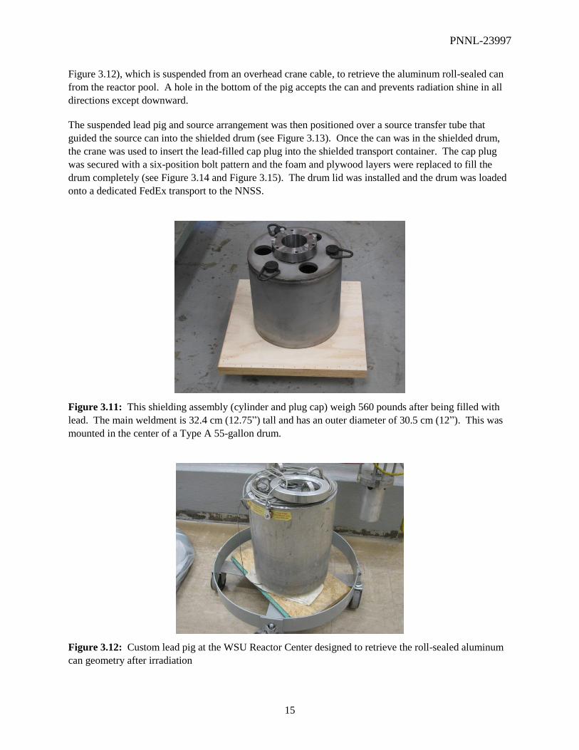
Figure 3.11: This shielding assembly (cylinder and plug cap) weigh 560 pounds after being
filled with lead. The main weldment is 12” tall and has an OD of 12.75”. This was mounted
in the center of a Type A 55-gallon drum. ................................................................................ 15
Figure 3.12: Custom lead pig at the WSU Reactor Center designed to retrieve the roll-sealed
aluminum can geometry after irradiation .................................................................................. 15

PNNL-23997
xiv
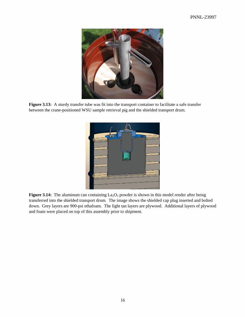
Figure 3.13: A sturdy transfer tube was fit into the transport container to facilitate a safe transfer
between the crane-positioned WSU sample retrieval pig and the shielded transport drum ...... 16
Figure 3.14: The aluminum can containing La2O3 powder is shown in this model render after
being transferred into the shielded transport drum. The image shows the shielded cap plug
inserted and bolted down. Grey layers are 900-psi ethafoam. The light tan layers are
plywood. Additional layers of plywood and foam were placed on top of this assembly prior
to shipment. ............................................................................................................................... 16
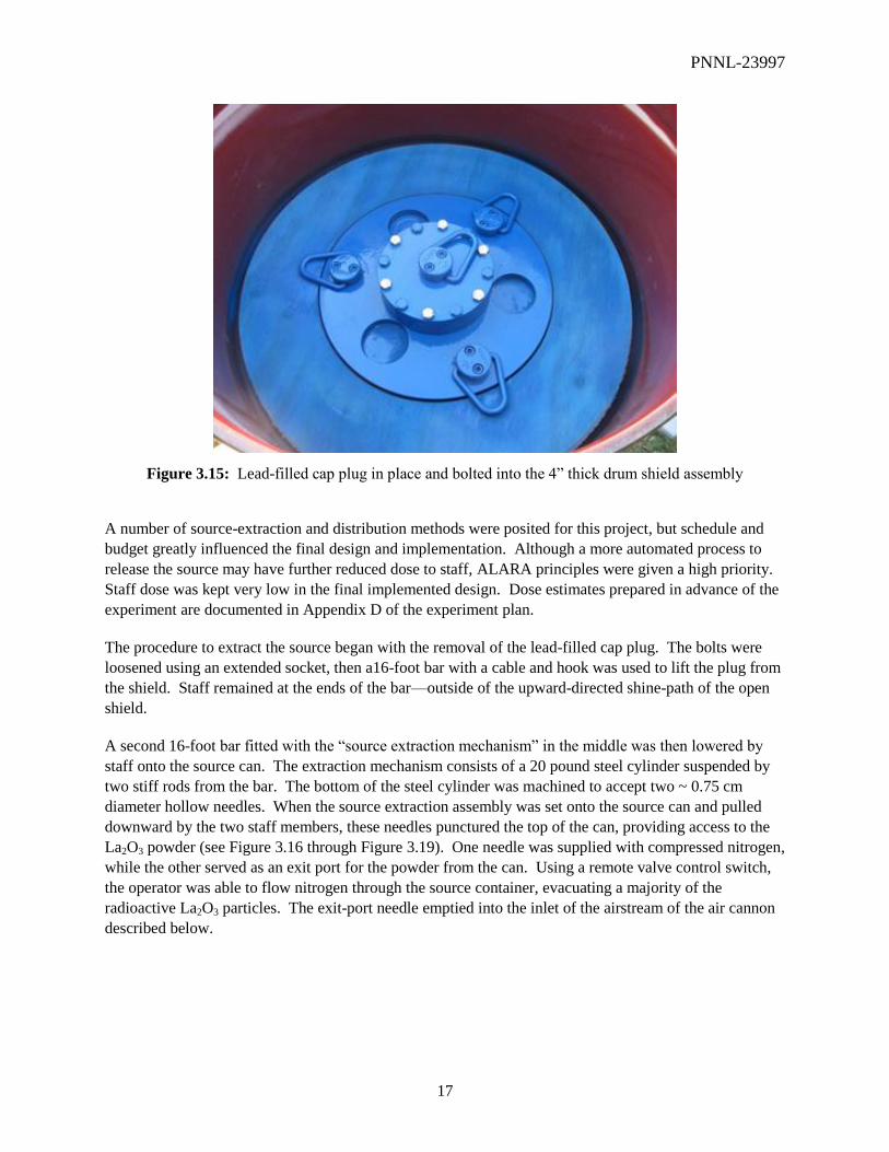
Figure 3.15: Lead-filled cap plug in place and bolted into the 4” thick drum shield assembly ...... 17
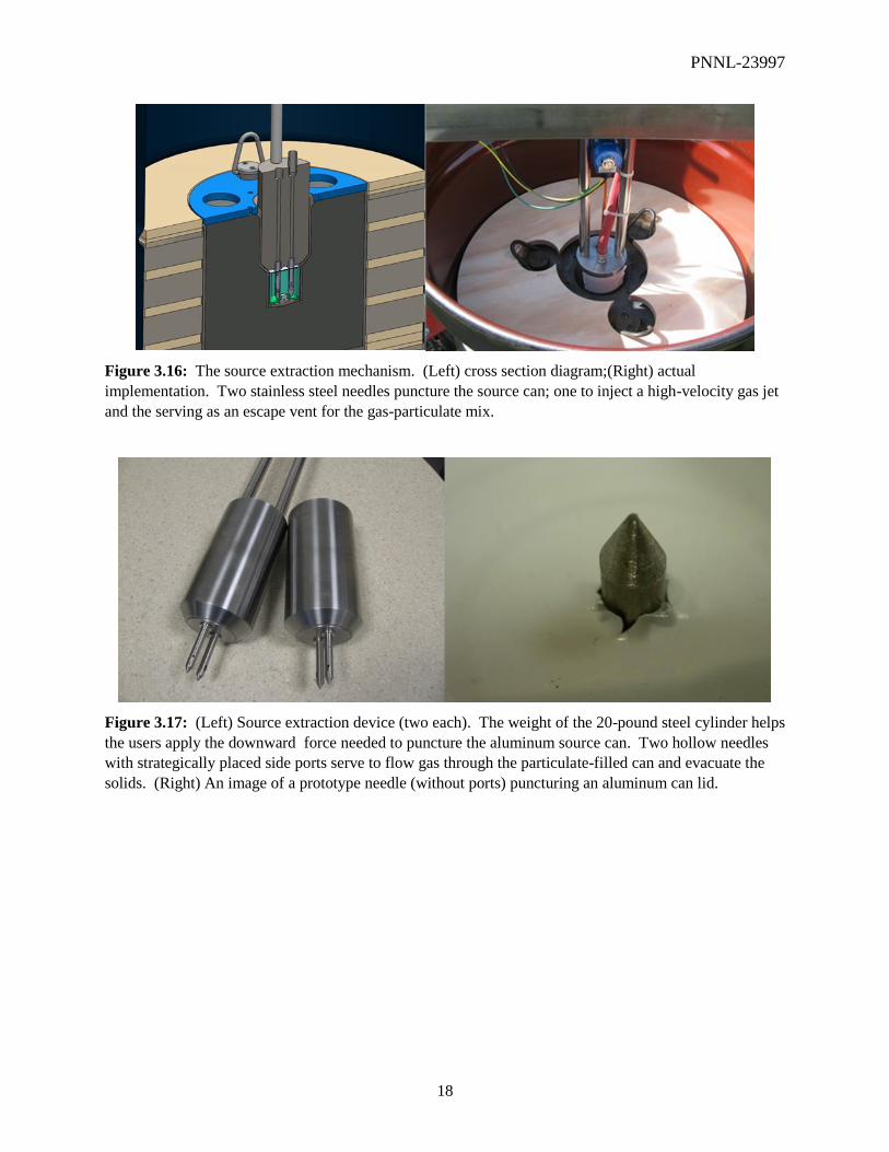
Figure 3.16: The source extraction mechanism. (Left) cross section diagram;(Right) actual
implementation. Two stainless steel needles puncture the source can; one to inject a high-
velocity gas jet and the serving as an escape vent for the gas-particulate mix. ........................ 18
Figure 3.17: (Left) Source extraction device (two each). The weight of the 20-pound steel
cylinder helps the users apply the downward force needed to puncture the aluminum source
can. Two hollow needles with strategically placed side ports serve to flow gas through the
particulate-filled can and evacuate the solids. (Right) An image of a prototype needle
(without ports) puncturing an aluminum can lid. ...................................................................... 18
Figure 3.18: A test can after being punctured by the source extraction system. (The can lid was
not roll-sealed for this test) ....................................................................................................... 19
Figure 3.19: Cross-Sectional view of the source shipping/transfer system. This image shows the
system with the source extraction plug installed. ..................................................................... 19
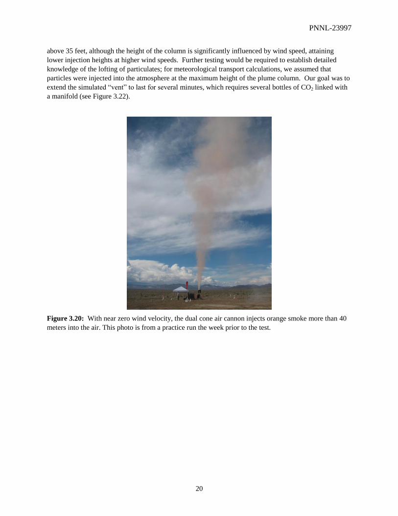
Figure 3.20: With near zero wind velocity, the dual cone air cannon injects orange smoke more
than 130 feet into the air. This photo is from a practice run the week prior to the test. ............ 20
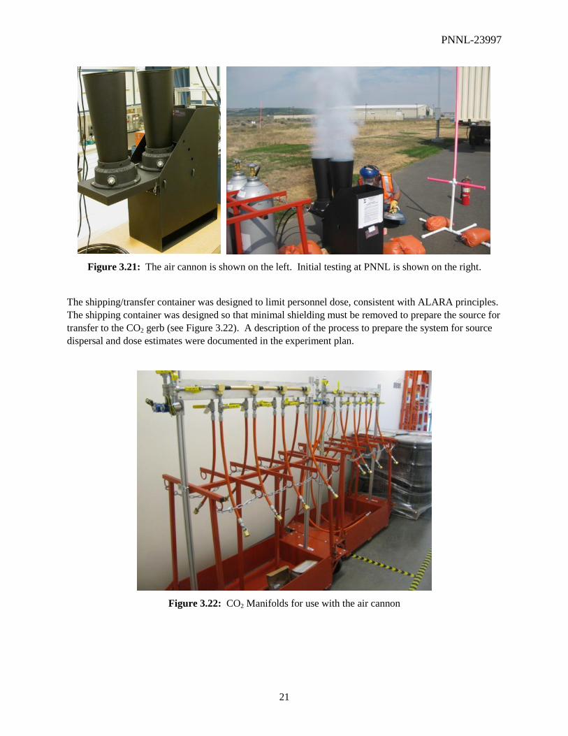
Figure 3.21: The air cannon is shown on the left. Initial testing at PNNL is shown on the right. . 21
Figure 3.22: CO2 Manifolds for use with the air cannon ................................................................ 21
Figure 3.23: Map of the planned locations for sampling sites. The dispersal point, marked
“GZ,” is located near the bottom center of the figure. The figure consists of a 50 m 50 m
grid; the yellow highlighted boxes are 1 km apart in the North-South direction, and 2 km
apart in the East-West direction. Points marked with a “1” had one of each type of witness
plate installed. Points marked with a “5” had five of each type of witness plate installed. ..... 23
Figure 3.24: Tacky mat witness plate staked for collection of lanthanum powder ......................... 24
Figure 3.25: Glass slide witness plate for the collection of microspheres ...................................... 25
Figure 3.26. Comprehensive sampling site. GZ is in the direction to the right. ............................ 26
Figure 3.27: Modified gasoline-powered leaf blower modified to operate as a 1000 cfm air
sampler, located 2 km downwind from the release. .................................................................. 27

PNNL-23997
xv
Figure 4.1: Surface weather map on May 14, 2013 at 1200Z. ........................................................ 28
Figure 4.2: Wind observations across the NTS site on May 14, 2013 10:45 a.m. .......................... 29
Figure 4.3: Balloon profiles of wind, temperature, and humidity pre-PRex release (i.e., May 14,
2013 10:45 a.m.) ....................................................................................................................... 31
Figure 4.4: Collection of tacky mat witness plate hampered by the bowed shape and the wind .... 33
Figure 4.5: Soil sampling with a trowel .......................................................................................... 34
Figure 4.6: Soil sampling with a tacky mat .................................................................................... 35
Figure 4.7: Soil sampling with battery-powered vacuum cleaner .................................................. 36
Figure 4.8: Survey equipment following the release of 140
La. The two NaI(Tl) detectors were
packaged in large Igloo coolers, and are next to each other, oriented front-to-back in the bed
of the Kawasaki Mule. .............................................................................................................. 37
Figure 4.9: Raven light bar (http://ravenprecision.com/products/guidance-steering/rgl-lightbar-
series)and the differential GPS unit (http://www.geneq.com/catalog/en/sxblue2.html) used to
guide the driver during vehicle ground survey. ........................................................................ 38
Figure 4.10: Hand-held radiation detectors used for in-situ measurements, atop a high-tech
detector stand ............................................................................................................................ 38
Figure 4.11: Thermo Packeye, a backpack PVT-based man-portable survey instrument .............. 39
Figure 4.12: B-200 performing aerial survey of 140
La release (left) and image of aircraft from an
AMS presentation (right) (Lyons 2012) ................................................................................... 40
Figure 4.13: Exterior of Quonset hut that housed the field laboratory for PRex. Note the liquid
nitrogen dewars provided for cooling of the HPGe detectors, on right. ................................... 41
Figure 4.14: Two ~50% relative efficiency HPGe detectors inside of 10.16 cm (4”) thick lead
shields. These detectors are set up in the field laboratory. ....................................................... 41
Figure 4.15: Single shield housing two 7.62 cm × 12.7 cm (3” × 5”) NaI(Tl) detectors. The
detectors are surrounded by 10.16 cm (4”) of lead, and the sample chambers are also
separated by 10.16 cm (4”) of lead. .......................................................................................... 42
Figure 4.16: Canberra HPGe with commercial portable shield system, supplied by NSTec. The
Canberra ISOCs efficiency calibration on this system was used to cross-calibrate the other
HPGe detectors. ........................................................................................................................ 42
Figure 5.1: RSI vehicle survey route using an ROI on the 140
La 1596 keV gamma. Count rates
are for two detectors, unintentionally multiplied by a factor of two because the system was
set up with a “virtual” detector that created a sum of the two individual NaI(Tl) detectors.
PNNL-23997
xvi
The plot shows the count rate for the sum of the two individual detectors, and the virtual
detector. This figure does not show the full extent of the survey to the North. ........................ 45
Figure 5.2: Gross counts detected by ground survey with the RSI system. The data is the sum of
two NaI(Tl) detectors. The color key is <5000 cps black, 5000 – <5500 cps blue, 5500-
<6000 cps green, 6000-<6500 yellow, ≥6500 red. ................................................................... 45
Figure 5.3: Gross Count contours of the RSI with two 2” × 4” × 16” NaI log detectors. .............. 46
Figure 5.4: Contours of the surveyed deposition based on 140
La using the count rate in the
1596-keV line ........................................................................................................................... 47
Figure 5.5: Gross counts versus dose for one NaI(Tl) detector ...................................................... 48
Figure 5.6: Comparison of vehicle and backpack transects of plume. The top (near sample area 1-
4) and bottom panel (near sample area 5-4) compare gross count (RSI) (RSI count rates are
doubled due to “virtual detector”) with dose rate (Packeye). The paths followed for the
Packeye and RSI surveys were close, but not precisely the same. ........................................... 51
Figure 5.7: Tacky mat (filled circles) overlaid on mobile survey contours of extracted 140
La ....... 55
Figure 5.8: Aerial mapping product showing gross count exposure ............................................... 57
Figure 5.9: Aerial mapping product showing plume results using an ROI over the 140
La
1596-keV line ........................................................................................................................... 58
Figure 5.10: Locations of handheld instrument comparisons. ........................................................ 60
Figure 5.11. Hotshot plume post-analysis assuming a 1 Ci release. The contours based on Hotshot
indicate that the measurable plume would have extended further downwind if the full 1 Ci
had been released. ..................................................................................................................... 63
Figure 5.12: Hotshot plume post-analysis assuming a 0.07 Ci release. The yellow push-pin
markers correspond to the in-situ measurement results provided in Table 5-3. The in-situ
measurements are generally in good agreement with the Hotshot contours. ............................ 64
Figure 5.13: Lanthanum oxide powder’s generally amorphous shape is visually indistinguishable
from ubiquitous desert airborne particulate. ............................................................................. 65
Figure 5.14: A color-enhanced micrograph of aluminosilicate glass microspheres on a test slide
similar to the witness plates deployed during the NCNS test. Concentric rings around each
sphere are the result of dark field lighting; and create a unique visual signature for the
microspheres compared to other debris also shown. ................................................................. 69
Figure 5.15: Micrograph of aluminosilicate glass microspheres in dark field illumination without
color enhancement .................................................................................................................... 69

PNNL-23997
xvii
Figure 5.16: Micrograph with bright field illumination of microspheres shown with red outlines
indicating identification by image recognition software. The software has identified all of
the microspheres in this field of view with the exception of the large sphere second from the
left. This sphere has agglomerated with another particle which has prevented identification.
Software filters can be set to be more tolerant of such interferences, but those settings can
also lead to false identifications. ............................................................................................... 70
Figure 5.17: Micrograph showing a roughly spherical pollen particle roughly the same size as
tested microspheres. This type of “background” particle, in certain microscope lighting
conditions, may be mistakenly identified by the image analysis software as a microsphere. .. 70
Figure 5.18: Left - Unidentified biological object. The outline of these bifurcated objects is
easily confused with a spherical object. They exhibit similar light reflections and circular
outline as microspheres. Right - Over the course of weeks, these objects were observed to
“grow” from generally circular to distinct two “pedal” forms. ................................................. 71
Figure 5.19: PAPR Air Sampler collections were consistent with the observed ground deposition72
Figure 5.20. Meteorological data from the weather station immediately south of the release point73
Figure 5.21. Meteorological data captured from the weather station immediately south of the
release point .............................................................................................................................. 74
Figure 5.22. Count rate (blue) and smoothed count rate (red) of a GM tube monitoring sample
collection 1.5 km downwind from the release. This sampler was remotely activated shortly
before the release, and the plume’s arrival can be observed during the sampling period. ........ 74

PNNL-23997
xviii
Tables
Table 3-1: La2O3 Sample Masses .................................................................................................... 11
Table 4-1: Meteorological Observations at Nearby Tower Locations on May 14, 2013 10:45
a.m. ........................................................................................................................................... 30
Table 5-1: Typical Values Extracted from Figure 6-3 .................................................................... 49
Table 5-2: Comparison of ROI and GC Counts in Spectra with and without 140
La ........................ 49
Table 5-4: Deposition Plume Width Estimate Based on Large Area Witness Plates ..................... 53
Table 5-5: Comparison of Tacky Mats and Mobile Survey ............................................................ 54
Table 5-3: Comparison of deposited activity measured by different instruments .......................... 61
Table 5-6: Table of MDAs for four detectors at 1 m height in terms of an infinite plane (modeled
as a uniform disk source 40 meters in diameter) for 10-minute acquisition times of 140
La’s
1596 keV Peak. ......................................................................................................................... 62
Table 5-7. Beads collected by Optical Witness Plates at Various Sampling Locations .................. 67

PNNL-23997
1
1.0 Introduction
The Comprehensive Nuclear-Test-Ban Treaty (CTBT) is a nuclear non-proliferation treaty adopted by the
United Nations and open for signature and ratification or accession by States Parties, but not yet entered
into force. The CTBT makes provision for a verification regime that includes the conduct of an On-Site
Inspection (OSI). The sole purpose of an OSI is to determine whether a nuclear explosion has occurred in
violation of the treaty and, if so, gather facts that might assist in identifying the violator. The Treaty
allows for an OSI to include many techniques, including the radionuclide techniques of gamma radiation
survey and spectrometry and environmental sampling and analysis (of solids, liquids, and gases). A good
understanding of the possible contamination distribution, along with the most valuable equipment and
search techniques for locating accessible radioactive contamination, would dramatically improve the
likelihood of conducting a successful OSI. In support of future OSIs, Pacific Northwest National
Laboratory (PNNL) conducted work to understand the realistic distribution of nuclides that might occur
under actual venting conditions from an underground nuclear test.
1.1 Background
OSI inspection teams will face restrictions in time and labor, as dictated by the CTBT, as well as likely
logistical difficulties. The OSI challenge that this experiment investigated is to locate limited radioactive
debris that has escaped an underground nuclear explosion and settled on the earth’s surface near and
downwind of ground zero (GZ). To support the understanding and selection of sampling and survey
techniques for use in an OSI, we designed this experiment to simulate a small-scale vent from an
underground nuclear explosion. This initial test used short-lived 140
La to provide a realistic ground
deposition pattern from a single vent location. The experiment afforded an opportunity to investigate
aerial and ground survey techniques, sampling OSI base-of-operations laboratory measurements, and the
associated minimum detectable activities (MDAs). The work also provided a data set that may prove
useful in future work to develop and benchmark local atmospheric transport models, and to develop
anomaly detection and information barrier algorithms.
This experiment examined the atmospheric dispersion and subsequent ground deposition of radioactive
particulates after injection into the atmosphere. During execution of the test, short-lived 140
La was
injected into the atmosphere from the ground to approximately a 35-foot altitude. The most viable
radionuclides originally considered for use in the test included 24
Na, 111
In, 140
La, and 198
Au. The test was
conducted within the Yucca Flats basin on the Nevada National Security Site (NNSS). The experiment
used particle sizes that 1) undergo atmospheric dispersion, and 2) have a high fraction of the particles
settle out over a distance of a few kilometers. The reasons for such particle sizes include health and
safety (strictly limiting the radioactive material transport to within the NNSS boundaries), cost and
logistics – the initial activity required to establish a desired ground deposition is kept to a minimum if the
particles do not transport long distances, and relevance to an OSI where the inspection team is attempting
to locate the ground deposition in the nearby vicinity of a test.
In order to gain information on the atmospheric transport and settling at known particle sizes, La2O3
powder was sieved to produce a sample with a narrow size distribution of particles. Additional non-
radioactive glass microspheres were also released; one secondary objective of the experiment was to
determine whether we are able to plot deposition contours using optical microscopy to measure the

PNNL-23997
2
deposition of microspheres collected on witness plates, and to compare the results of this method to
deposition contours determined via radiation survey methods. This portion of the effort is interesting
because it could enable significant further study of local transport related to vented underground nuclear
explosions without the significant logistics efforts required for a radioactive release.
1.2 Objective
The objective of the particle release experiment (PRex) was to simulate a small-scale vent from an
underground test, and to measure this release using an array of sampling/survey equipment and
techniques. One of the challenges in an OSI is to locate radioactive debris that has escaped an
underground nuclear explosion and settled on the surface near and downwind of GZ. Successful search
and identification of such debris will enable inspectors to confirm that a nuclear test occurred. Positive
results will also enable the inspection team to locate the testing site. To develop a robust OSI capability,
it is necessary to understand the surface source term created by intermediate and long half-life (t1/2 in the
weeks to years range) particulate nuclear explosion debris. To facilitate study of the source term without
the attendant long-term contamination associated with mixed fission products, this experiment used a
shorter-lived radionuclide (140
La t1/2 = 1.678 days). The data acquired in this experiment will be used to:
Quantify how different sampling/survey methods affect minimum detectable activities (MDAs)
Evaluate local variability of vented fallout
Support development of local atmospheric models (ATMs) to enable prediction of source terms
Support studies of anomaly detection/information barrier algorithms
Successful execution of this experiment has also further advanced the capability of NNSS to perform
particulate radiological release studies.
1.3 Scope of Document
This report documents the execution, data collection, and analysis results for the PRex release, which
occurred at 10:55 a.m. on Tuesday, May 14th, 2013. Specifically, the following aspects of the PRex
experiment are discussed:
Pre-release preparation: including site selection, source production and transport to the experiment
site, dispersal mechanism, and simulations to predict the extent of dispersal
On-site preparation: pre-event radiological survey, infrastructure, and pre-established contamination
areas
Set-up and execution of the dispersal event: including transport of the source to the site, assembly of
the release mechanism, and meteorological conditions experienced during the test
Data collection: an overview of the data collection tasks and systems used
Data analysis and results
Lessons Learned
PNNL-23997
3
2.0 Experimental Considerations
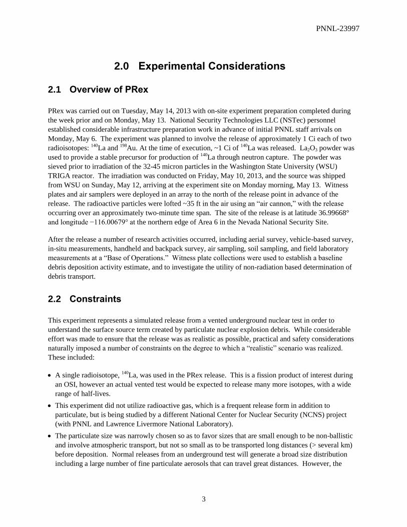
2.1 Overview of PRex
PRex was carried out on Tuesday, May 14, 2013 with on-site experiment preparation completed during
the week prior and on Monday, May 13. National Security Technologies LLC (NSTec) personnel
established considerable infrastructure preparation work in advance of initial PNNL staff arrivals on
Monday, May 6. The experiment was planned to involve the release of approximately 1 Ci each of two
radioisotopes: 140
La and 198
Au. At the time of execution, ~1 Ci of 140
La was released. La2O3 powder was
used to provide a stable precursor for production of 140
La through neutron capture. The powder was
sieved prior to irradiation of the 32-45 micron particles in the Washington State University (WSU)
TRIGA reactor. The irradiation was conducted on Friday, May 10, 2013, and the source was shipped
from WSU on Sunday, May 12, arriving at the experiment site on Monday morning, May 13. Witness
plates and air samplers were deployed in an array to the north of the release point in advance of the
release. The radioactive particles were lofted ~35 ft in the air using an “air cannon,” with the release
occurring over an approximately two-minute time span. The site of the release is at latitude 36.99668°
and longitude −116.00679° at the northern edge of Area 6 in the Nevada National Security Site.
After the release a number of research activities occurred, including aerial survey, vehicle-based survey,
in-situ measurements, handheld and backpack survey, air sampling, soil sampling, and field laboratory
measurements at a “Base of Operations.” Witness plate collections were used to establish a baseline
debris deposition activity estimate, and to investigate the utility of non-radiation based determination of
debris transport.
2.2 Constraints
This experiment represents a simulated release from a vented underground nuclear test in order to
understand the surface source term created by particulate nuclear explosion debris. While considerable
effort was made to ensure that the release was as realistic as possible, practical and safety considerations
naturally imposed a number of constraints on the degree to which a “realistic” scenario was realized.
These included:
A single radioisotope, 140
La, was used in the PRex release. This is a fission product of interest during
an OSI, however an actual vented test would be expected to release many more isotopes, with a wide
range of half-lives.
This experiment did not utilize radioactive gas, which is a frequent release form in addition to
particulate, but is being studied by a different National Center for Nuclear Security (NCNS) project
(with PNNL and Lawrence Livermore National Laboratory).
The particulate size was narrowly chosen so as to favor sizes that are small enough to be non-ballistic
and involve atmospheric transport, but not so small as to be transported long distances (> several km)
before deposition. Normal releases from an underground test will generate a broad size distribution
including a large number of fine particulate aerosols that can travel great distances. However, the

PNNL-23997
4
logistics of producing and transporting the radioactive source material dictated that we narrow the size
distribution to ensure deposition in the near-field.
The ~40 micron particle size was also chosen to be above the size typically considered respirable.
The location of the trial may not be representative of a broad range of test site environments. While
the experiment was performed at the former Nevada Test Site (where underground nuclear explosions
did take place), the specific site selected for the release was chosen in part for environmental conditions
that allowed for a favorable release and relative ease of post-release survey/sampling.
2.3 Assumptions
The experiment plan was originally developed using the following assumptions:
Nearly 100% of the source material will be lofted by the “air cannon” (also referred to as the CO2 gerb
in this document)
The release mechanism will loft the source material ~35 m into the air with wind speeds at the low end
of the acceptable parameters, and ~15 m into the air with wind speeds at the high end of acceptable
parameters. With favorable meteorological conditions, this material will be deposited within a
“contamination area” roughly 2–4 km (downwind) 0.5 km (crosswind) in size.
All equipment used for data collection will be in good working order, including having passed
calibration checks within the past year (or other period recommended by the manufacturer). It is not
assumed that instruments will be calibrated specifically for isotopes used in the test.
Favorable weather conditions within a 3-day period between 8 a.m. and 5 p.m. are likely
2.4 Pre-Execution Release Parameters
The following parameters were established prior to the experiment and are summarized here for easy
reference. Several are addressed in more detail later in this document, and a detailed description of the
release parameters is available in the experiment plan.
Location: The experiment was held at the northern edge of Area 6 in the Nevada National Security
Site (NNSS). Coordinates for the release site are (see Figure 2.1):
– Lat/Long: 36.99668°, −116.00679°
Timing: The window for release was 8 a.m. – 5 p.m., Tuesday, May 14th through Thursday, May 16
th,
2013. The actual release began at ~10:55 a.m. on Tuesday, May 14th, 2013, with a duration of
approximately 1 to 2 minutes.
Source configuration:
– Release mechanism: Continuous Flow Confetti Gerb Launcher (“Air Cannon”)
– Source material: approximately 1 Ci of 140
La
Meteorological conditions: Acceptable meteorological conditions for the test were documented in the
PRex Experiment Plan (Seifert et al. 2013)

PNNL-23997
5
Figure 2.1: PRex test location on the Nevada National Security Site

PNNL-23997
6
3.0 PRex Experiment Preparation
3.1 Experiment Plan
The PRex Experiment Plan (Seifert et al. 2013) provides many of the details used in site selection,
radioisotope selection, meteorological planning, required test site infrastructure, dose estimates, and pre-
event concept of the sequence of events. Much of the information is not repeated in this document, and
the reader is referred to the experiment plan for specifics on planning the experiment.
3.2 Site Selection
A number of possible sites at the NNSS were visited in January 2012 for determining the ideal site for
PRex. Our initial desired criteria list was as follows:
1. A pristine (little radiological background from previous Test Site activities) location far enough from
site infrastructure and borders so as not to be a health issue. Several square kilometers, including
access roads, would need to be temporarily closed off.
2. Nearby and downwind, there should be an area that does have radiological background from previous
tests. This is important so that data can be taken to test algorithms and procedures that can
discriminate fresh tests from old tests under a CTBT OSI.
3. At least part of the downwind area should be accessible for vehicle radiation surveys so that
procedures and equipment can be tested relative to OSI techniques
4. As close to Mercury as reasonable, with infrastructure like electricity, if available
5. Preferably, the area should be chemically as well as radiologically pristine because some of the
research tools employed may be based on chemical analysis
We did not have sufficient information to investigate criterion 5 during our visits. There appeared to be
no suitable locations with access to electricity, forcing the use of a generator during the test. In the end,
criteria 3 and 4 trumped criterion 2 and a site in the northern end of Area 6 was chosen at latitude
36.99668° and longitude −116.00679°. The site is at the southern end of the Yucca Flats area,
immediately to the south of where many underground nuclear tests occurred in the past, but on the eastern
edge away from the main road (Mercury Highway). Likewise, the Area 6 Construction Support Facilities
area and Control Point are a few miles away to the southwest, but not downwind of the planned release.
The location is very flat with light desert grass and small shrubs, providing for straight-forward off-road
and aerial survey (see Figure 3.1). Although there are radiologically-controlled areas downwind of the
release site, particularly those associated with the tests Adze and Seaweed, these do not have surface
radiation from old tests but are fenced to prevent the disturbance of buried contamination.
PNNL-23997
7
Figure 3.1: NNSS release site. While not visible in the photo, several craters and un-collapsed test
locations exist in close proximity to the north of the planned release point. Craters are more concentrated
to the northwest; south-southwesterly winds would result in the fewest obstacles for ground survey.
3.3 Background Measurements, September and October 2012
A vehicle-based background survey was performed in advance of the test using an RSI RS 700
spectrometer system with two 5.08 cm × 10.16 cm × 40.64 cm (2″×4″×16″) NaI(Tl) detectors mounted in
the bed of a Kawasaki Mule All-Terrain Vehicle (ATV). The RS 700 has an integrated global positioning
system (GPS) that recorded coordinates along the path where the ATV was driven. An additional
guidance system was tested in conjunction with the built-in GPS. A Raven RGL 600 system, originally
designed to guide the precision driving of agricultural equipment, and an ancillary GPS unit were
combined to enable driving parallel lines of arbitrary separation starting from two points determined by
the user.
On September 25th and 26
th, 2012, staff members from PNNL performed a vehicle-based survey of the
proposed PRex release site using the equipment described above. The survey was intended to provide a
baseline for comparison with post-release measurements. This vehicle survey also served to identify
whether the several-square–kilometer site would present complications not previously spotted from the
road. Parallel lines of increasing length (as the vehicle moved further from the release point) were driven
with the help of the Raven RGL 600 system and ancillary GPS. The ATV was driven at a nominal
3 mph, with line spacings of 50 m (closest to the release point) and 100 m (~1 km and further). The data
was retrieved both from the cabin system (laptop computer) and directly from the RS 700 unit. A sample
of the data is shown in Figure 3.2. The final configuration of the vehicle and a contour map of the vehicle
survey results are shown in Figure 3.3.

PNNL-23997
8
Figure 3.2: Screen capture made with the RSI Software RadAssist and a GIS module showing raw data
from the September 2012 background survey
Figure 3.3: ATV used for vehicle survey at the PRex location on Yucca Flats (left); contour map of
radiation survey results (right)
On October 15, 2012, NNSA’s Aerial Measuring System (AMS) flew a Radiation Solutions, Inc. (RSI)
array of 12 NaI(Tl) detectors over the planned site of the NCNS PRex. These flights were conducted to
assess the initial radiological conditions of the experiment site, including areas where short-lived
radioactivity was expected to deposit on the ground during the experiment. The AMS System was flown

PNNL-23997
9
at 70 knots, 50 feet in elevation, and 75-foot line spacing. The exposure map produced is shown in
Figure 3.4.
Figure 3.4: Gross count exposure map measured over the PRex release area in October 2012
3.4 Source Production
3.4.1 Preparation of La2O3 Powder
Lanthanum oxide, La2O3, was purchased from Materion at 99.99% purity and -200 mesh. The material
was separated by particle size using a Retsch AS200 sieve shaker (Figure 3.5 and Figure 3.6). The sieves
purchased included No 230 (63 µm), No 270 (53 µm), No 325 (45 µm), No 450 (32 µm), and No 500
(25 µm). The resulting particle size ranges were > 63, 53-63, 45-53, 32-45, 25-32, and < 25 µm. Chains
were used to aid the sieving process. After sieving, the material selected for irradiation and release was in
the 32-45 µm range. In preparation for sieving, the sieves, chains, and lid were washed with alcohol by
spraying the part, allowing the alcohol to run down the part, repeating the alcohol rinse, then drying the
part in a flow hood. The shaker table, base of the glove bag, and balance were covered in 1.5-mil
aluminum foil. La2O3 is hydroscopic; the sieving process was done in a nitrogen-filled disposable glove
bag, see Figure 3.5 and Figure 3.6 to prevent the adsorption of water.. The glove bag was inflated at
20 psi and then purged at 100 cc/min for 3 days.

PNNL-23997
10
Following sieving, material in each sieve was carefully poured into an aluminum foil pocket from which
it could then be poured into sample containers. The La2O3 in each sieve was split between two pre-
weighed glass jars and the final weight recorded while in the glove bag. The jars were then sealed with
vinyl tape and removed from the glove bag. Scoopulas were used to aid in material transfer and to take
sub-samples for analysis. To minimize the spread of different particle size material in the glove bag, a
different aluminum pocket and a new individually wrapped scoopula was used for each sample. In
addition to the material stored in the glass jars, a small sample was taken for irradiation at the WSU
TRIGA reactor to verify purity. Sub-samples were stored in 20-mL poly liquid scintillation counter vials.
See Table 3-1 for samples generated with associated masses.
Figure 3.5: Shaker / sieve setup including shaker, sieves, balance, and sample jars in a
nitrogen filled glove bag
Figure 3.6: Shaker and sieves are shown on the left. The sieve cover with La2O3 powder
is shown on the right.

PNNL-23997
11
Table 3-1: La2O3 Sample Masses
Particle Sizes
Jar
Designation
Tare
(grams)
with La2O3
(grams)
Final weight
(grams)
jar with lid jar w/o lid jar w/ lid
25 - 32 A 215.9 203.66 287.875 71.975
25 - 32 B 214.3 201.91 294.818 80.518
45 - 32 A 215.87 203.71 327.3 111.43 material
for release
45 - 32 B 215.81 203.57 332.481 116.671
WSU A vial 7.01 5.14 14.455 7.445
25 - 32 vial 7 7.597 0.597
WSU B vial 6.99 5.11 6.999 0.009
WSU C vial 7 9.393 2.393 shipped to
WSU
53 - 45 vial 7 9.204 2.204
53 - 45 A 215.57 203.44 269.145 53.575
53 - 45 B 214.73 202.42 284.202 69.472
63 - 53 vial 7 9.075 2.075
63 - 53 A 216 203.67 280.692 64.692
63 - 53 B 214.29 301.95 284.963 70.673
bottom catch pan 213.94 201.89 approximately
20 g
approximate masses - vial not tared

PNNL-23997
12
3.4.2 Irradiation at Washington State University
The lanthanum oxide powder was irradiated in double containment in position D8 of the WSU TRIGA
research reactor. The 36 minute irradiation was performed on Friday, May 10 with a target 140
La
production of 2.2 Ci at noon Pacific daylight time (PDT) on Sunday, May 12. The irradiation was
performed at 1 MW, with a neutron flux previously characterized as 5.3×10¹²
n/cm2/sec
2. Gamma assay
performed after the irradiation confirmed production of the desired 140
La activity.
Prior to irradiation, the WSU Reactor Center Safety Committee, with input from PNNL, determined that
the lanthanum oxide powder is a dispersible material. WSU had previously approved a roll-sealed
aluminum can geometry (Figure 3.7) for irradiation of non-dispersible material; they subsequently
requested additional measures to ensure containment of the dispersible La2O3 powder. To satisfy these
requirements, PNNL designed an aluminum liner (Figure 3.8) to fit inside the roll-sealed drawn
aluminum cans. One challenge was to design the liner to be tough enough to withstand drop forces, yet
still present a section thin enough to allow puncture by the powder extraction needles. The liner was
fabricated, tested and showed the expected deformation resulting from a 20-foot drop test onto a concrete
floor (Figure 3.9). PNNL submitted a report on the change of design and associated experiments (Smart
2013) to the reactor safety committee, which granted permission to proceed with the irradiation using the
nested can liner and aluminum roll sealed can (Figure 3.10).
Figure 3.7: The roll-sealed aluminum can provided by the WSU Reactor Center team. This can has been
certified by the reactor center for use with non-dispersible materials. PNNL leveraged the “certified”
status of this geometry as well as the geometry specific insertion and retrieval equipment already in place
at the reactor center.

PNNL-23997
13
Figure 3.8: The 6061-T6 aluminum liner assembly. Light blue section includes a thin septum end with
appropriate reinforcement areas to reduce stress. Green section is the welded end cap with a 1/2" 20-
threaded plug. The light purple area is a high density polyethylene plug gasket.
Figure 3.9: A 20-foot drop test conducted with a water-filled aluminum “can liner” resulted in the
expected amount of deformation, with no rupture or leakage
PNNL-23997
14
Figure 3.10: The “roll-sealed aluminum can” with the custom designed aluminum liner inside. The
aluminum liner has a thin annulus around its top wall to allow puncture by the material extraction needles.
3.4.3 Source Transport
The design and fabrication of the shipping container took place in advance of the final experiment design.
The transport shielding was designed based on 2.5 Ci of 140
La activity at the time of pick-up by the
shipping company. Monte Carlo N-Particle (MCNP ) Version 5 (Forster et al. 2004) transport
calculations showed that if centered in a type “A” 55-gallon drum, that 4 in. of lead shielding around the
source would reduce drum surface dose to less than 200 mrem/hr; which is below a “Yellow III” transport
maximum surface dose level. A lesser source strength of 1 Ci centered in a type A drum with 4 in. of lead
shielding would result in a surface maximum surface dose of less than 50 mrem/hr, which meets the
requirement for a “Yellow II” shipment.
A custom designed lead shield (see Figure 3.11) mounted in the center of a type A 55-gallon transport
drum reduced dose at the surface of the drum during transport, and held the source can in position during
the source extraction process. The 30.5 cm (12”) diameter by 32.4 cm (12.75”) tall steel encased lead
shield weighs about 560 pounds with the shielded top plug installed. The shield is supported in the center
of the drum with a system of 5/8” plywood rings and disks, layered with 2–in. thick, 900-psi ethafoam
sheets. The shield has three lift points used for installation into the drum.
After completing the irradiation, staff at the WSU reactor center loaded the irradiated source can into the
shielded transport drum. After removing the drum lid and the top layers of foam and plywood, the
exposed lead-filled cap plug was unbolted and removed. WSU staff used their existing lead pig (see
PNNL-23997
15
Figure 3.12), which is suspended from an overhead crane cable, to retrieve the aluminum roll-sealed can
from the reactor pool. A hole in the bottom of the pig accepts the can and prevents radiation shine in all
directions except downward.
The suspended lead pig and source arrangement was then positioned over a source transfer tube that
guided the source can into the shielded drum (see Figure 3.13). Once the can was in the shielded drum,
the crane was used to insert the lead-filled cap plug into the shielded transport container. The cap plug
was secured with a six-position bolt pattern and the foam and plywood layers were replaced to fill the
drum completely (see Figure 3.14 and Figure 3.15). The drum lid was installed and the drum was loaded
onto a dedicated FedEx transport to the NNSS.
Figure 3.11: This shielding assembly (cylinder and plug cap) weigh 560 pounds after being filled with
lead. The main weldment is 32.4 cm (12.75”) tall and has an outer diameter of 30.5 cm (12”). This was
mounted in the center of a Type A 55-gallon drum.
Figure 3.12: Custom lead pig at the WSU Reactor Center designed to retrieve the roll-sealed aluminum
can geometry after irradiation
PNNL-23997
16
Figure 3.13: A sturdy transfer tube was fit into the transport container to facilitate a safe transfer
between the crane-positioned WSU sample retrieval pig and the shielded transport drum.
Figure 3.14: The aluminum can containing La2O3 powder is shown in this model render after being
transferred into the shielded transport drum. The image shows the shielded cap plug inserted and bolted
down. Grey layers are 900-psi ethafoam. The light tan layers are plywood. Additional layers of plywood
and foam were placed on top of this assembly prior to shipment.
PNNL-23997
17
Figure 3.15: Lead-filled cap plug in place and bolted into the 4” thick drum shield assembly
A number of source-extraction and distribution methods were posited for this project, but schedule and
budget greatly influenced the final design and implementation. Although a more automated process to
release the source may have further reduced dose to staff, ALARA principles were given a high priority.
Staff dose was kept very low in the final implemented design. Dose estimates prepared in advance of the
experiment are documented in Appendix D of the experiment plan.
The procedure to extract the source began with the removal of the lead-filled cap plug. The bolts were
loosened using an extended socket, then a16-foot bar with a cable and hook was used to lift the plug from
the shield. Staff remained at the ends of the bar—outside of the upward-directed shine-path of the open
shield.
A second 16-foot bar fitted with the “source extraction mechanism” in the middle was then lowered by
staff onto the source can. The extraction mechanism consists of a 20 pound steel cylinder suspended by
two stiff rods from the bar. The bottom of the steel cylinder was machined to accept two ~ 0.75 cm
diameter hollow needles. When the source extraction assembly was set onto the source can and pulled
downward by the two staff members, these needles punctured the top of the can, providing access to the
La2O3 powder (see Figure 3.16 through Figure 3.19). One needle was supplied with compressed nitrogen,
while the other served as an exit port for the powder from the can. Using a remote valve control switch,
the operator was able to flow nitrogen through the source container, evacuating a majority of the
radioactive La2O3 particles. The exit-port needle emptied into the inlet of the airstream of the air cannon
described below.
PNNL-23997
18
Figure 3.16: The source extraction mechanism. (Left) cross section diagram;(Right) actual
implementation. Two stainless steel needles puncture the source can; one to inject a high-velocity gas jet
and the serving as an escape vent for the gas-particulate mix.
Figure 3.17: (Left) Source extraction device (two each). The weight of the 20-pound steel cylinder helps
the users apply the downward force needed to puncture the aluminum source can. Two hollow needles
with strategically placed side ports serve to flow gas through the particulate-filled can and evacuate the
solids. (Right) An image of a prototype needle (without ports) puncturing an aluminum can lid.

PNNL-23997
19
Figure 3.18: A test can after being punctured by the source extraction system. (The can lid was not roll-
sealed for this test)
Figure 3.19: Cross-Sectional view of the source shipping/transfer system. This image shows the system
with the source extraction plug installed.
3.5 Release Mechanism
PRex used an air cannon device (see Figure 3.21) expected to loft particulate materials over 35 m into the
air at the lower acceptable limit of wind speed (1.8 m/s or 4 mph), and ~15 m into the air at the high
acceptable limit of wind speed (6.7 m/s or 15 mph). This type of air cannon is powered with liquid CO2,
and utilizes the Coanda effect created by a nozzle structure and expansion of the CO2 into gas to produce
an upward-moving air column. Initial testing at PNNL indicated that the device lofts air and materials to
PNNL-23997
20
above 35 feet, although the height of the column is significantly influenced by wind speed, attaining
lower injection heights at higher wind speeds. Further testing would be required to establish detailed
knowledge of the lofting of particulates; for meteorological transport calculations, we assumed that
particles were injected into the atmosphere at the maximum height of the plume column. Our goal was to
extend the simulated “vent” to last for several minutes, which requires several bottles of CO2 linked with
a manifold (see Figure 3.22).
Figure 3.20: With near zero wind velocity, the dual cone air cannon injects orange smoke more than 40
meters into the air. This photo is from a practice run the week prior to the test.
PNNL-23997
21
Figure 3.21: The air cannon is shown on the left. Initial testing at PNNL is shown on the right.
The shipping/transfer container was designed to limit personnel dose, consistent with ALARA principles.
The shipping container was designed so that minimal shielding must be removed to prepare the source for
transfer to the CO2 gerb (see Figure 3.22). A description of the process to prepare the system for source
dispersal and dose estimates were documented in the experiment plan.
Figure 3.22: CO2 Manifolds for use with the air cannon

PNNL-23997
22
3.6 Meteorology Planning and Modeling
Details of the meteorological planning and modeling accomplished in preparation for the test are
documented in the PRex Experiment Plan.
3.7 NNSS Experiment Site Preparation
3.7.1 Posting Contamination and High Contamination Areas
NSTec personnel posted Contamination Area signs to encompass a rectangular region extending 1 km
east, 1 km west, 5 km north, and 0.5 km south of the dispersal point. High Contamination Area (HCA)
signs were posted around a rectangular area extending 0.1 km east, 0.1 km west, 0.5 km north, and 0.1 km
south of the dispersal point. The immediate area surrounding the dispersal system (~20 m × 20 m) was
enclosed in a temporary flexible orange fence to prevent unintended re-entry into the area. “Stomp and
Tromp” surveys performed by NSTec Radiological Control Technicians (RCTs) indicated that deposition
levels of 140
La did not reach HCA levels outside of the immediate fenced area of the dispersal system.
3.7.2 Prepositioned Sampling
In the days leading up to the experiment, sampling equipment was placed at predetermined locations and
prepared for collection of PRex plume debris. The plume sampling network consisted of both air
samplers and witness plates for the collection of debris. Two types of witness plates were used; one for
the collection of the radioactive lanthanum oxide powder and the other for collection of glass
microspheres. The radioactive measurements were performed quickly on site before decay of the 140
La
would make it undetectable; the glass microspheres were examined at a later time at PNNL.
3.7.2.1 Witness Plate Array
The witness plates were placed downwind at nearly 110 locations in a pattern similar to that shown in
Figure 3.23. The figure shows the planned, advance placement pattern; some of the locations were
modified due to the presence of craters or fenced off areas. The actual sampling locations are captured in
the data files. Since the exact path the radioactive plume would take was unknown, it was necessary to
cover the range of allowed plume directions. This was done with the expectation that many of the
sampling locations would not collect positive samples. It was recognized in advance that some samples
would be excluded from radiation measurement based on knowledge of the actual plume axis. The slight
skewing of the sample locations to the east of GZ reflects the same skewing in the range of acceptable
release wind directions, as documented in the experiment plan. This range of acceptable wind directions
was influenced by the presence of Mercury Highway to the west of the release. The sample locations in
many West-East rows are offset relative to other rows to reduce the risk of a narrow plume missing most
sampling points. One of each type of witness plate was placed at the locations designated with a “1.”
Those marked with a “5” had five of each type placed in the manner described below. Air samplers were

PNNL-23997
23
also placed at some of these locations, as described later in this document. After the release, several of
the “5” locations were also used as soil sampling locations. In situ measurements using various radiation
survey instruments were also taken at selected sampling locations after the release.
Figure 3.23: Map of the planned locations for sampling sites. The dispersal point, marked “GZ,” is
located near the bottom center of the figure. The figure consists of a 50 m 50 m grid; the yellow
highlighted boxes are 1 km apart in the North-South direction, and 2 km apart in the East-West direction.
Points marked with a “1” had one of each type of witness plate installed. Points marked with a “5” had
five of each type of witness plate installed.
3.7.2.1.1 Witness Plates for the Collection of Radioactive Powder
To collect radioactive lanthanum oxide powder for rapid measurement, large-area witness plates
comprised of “tacky mats” adhered to foam-core board were staked to the ground with aluminum tent
stakes (see Figure 3.24). The tacky mats used were 45.7 cm × 76.2 cm Criti Clean CRN-1836-30. Each
large-area witness plate included several layers of tacky mat material, with the top-most layer being non-
sticky material so they could be stacked for handling prior to placement. Placement of the witness plates
(these and the ones for microsphere collection described next) took several days. The large area witness
plates were placed lengthwise in the North-South direction and staking them to the ground usually
resulted in a slight bowing in the shorter East-West direction. The day before the release, the top non-
sticky layer was removed from the tacky mats so that they would be ready for collection. (The
southernmost rows—those closest to the release point—were not uncovered until the morning of the
release; there was insufficient time to uncover all 100+ sites on the morning of the test). The tacky mats

PNNL-23997
24
were not so sticky as to collect the very numerous grasshoppers, though some small black flies were
collected. To ease sample collection, the sampling sites were marked with bright orange ribbon on
wooden stakes.
Figure 3.24: Tacky mat witness plate staked for collection of lanthanum powder
3.7.2.1.2 Witness Plates for the Collection of Glass Microspheres
To collect the nonradioactive glass microspheres, 5.08 cm × 7.62 cm glass microscope slides were given
an adhesive top layer using double-sided tape (see Figure 3.25). The tape backing remained on the top of
the tape (and slide) when the witness plates were placed in the field, but was scored for easy removal
later. The bottom of the witness plates were taped to garden stakes in the field sampling locations after
the stakes had been placed at the appropriate locations. Grey duct tape was selected to secure the glass
slides to the garden stakes; this tape choice held tenaciously to the glass and unfortunately could not be
removed for the later analysis step. The height of the glass witness plates was approximately 30” above
the ground. In conjunction with the large tacky-mat witness plates, these microsphere witness plates had
their protective top backing removed the day before or morning before the release, depending on location.

PNNL-23997
25
Figure 3.25: Glass slide witness plate for the collection of microspheres

PNNL-23997
26
3.7.2.1.3 Comprehensive Sampling Sites
As noted earlier, some of the sampling sites had five of each type of witness plate. The purpose of this
was to investigate deposition variability on the order of a few meters. The five witness plates (of each
type) were placed in a “+” pattern, with the ends of the “+” pointing in the four cardinal directions and the
distance from each end to the center of the “+” being 3 m (see Figure 3.26). The glass microsphere
witness plates (in all cases and not just for the comprehensive sites) were placed just north of their
corresponding tacky mat witness plate. Samples were numbered by their primary site number and
appended with a position 1 through 5 (with 1 in the center, 2 to the west, 3 to the north, 4 to the east, and
5 to the south). For example, comprehensive sampling site 7-3 had large area witness plate samples
labeled 7-3-1 through 7-3-5.
Figure 3.26. Comprehensive sampling site. GZ is in the direction to the right.
3.7.2.2 Air Sampler Placement
Three different types of air samplers were set up to collect the radioactive tracer. Six air samplers with
1000 cubic feet per (cfm) minute capacity were set out as follows:

PNNL-23997
27
Two battery–powered, radio-controlled units were set up near the center line at 1.5 km down range.
These units were activated just before the release and ran for 20 minutes.
Four large gas-powered leaf blowers with modified intakes holding filter material were located two km
down range (see Figure 3.27). The high volume blowers used were used previously in Canada for a
similar tracer release study.
Seventeen powered air-purifying respirators (PAPR) with 17 lpm airflow were located along the 400-
and 500-m down range transects.
Figure 3.27: Gasoline-powered leaf blower modified to operate as a 1000 cfm air sampler, located 2 km
downwind from the release.
PNNL-23997
28
4.0 PRex Experiment Execution
4.1 Time and Location
The PRex release began at ~10:55 a.m. on Tuesday, May 14th, 2013, with a duration of approximately 1-
2 minutes. The release system did not contain an on-board radiation monitor, so the exact time period
over which the material was released is not known. The supply of nitrogen carrier gas was cycled on and
off several times during the first minute of the release, then was left flowing (on) for several minutes.
The experiment was held at the northern edge of Area 6 in the Nevada National Security Site.
Coordinates for the release site are 36.99668°N, 116.00679°W (see Figure 2.1). A log of events is
provided in Appendix C.
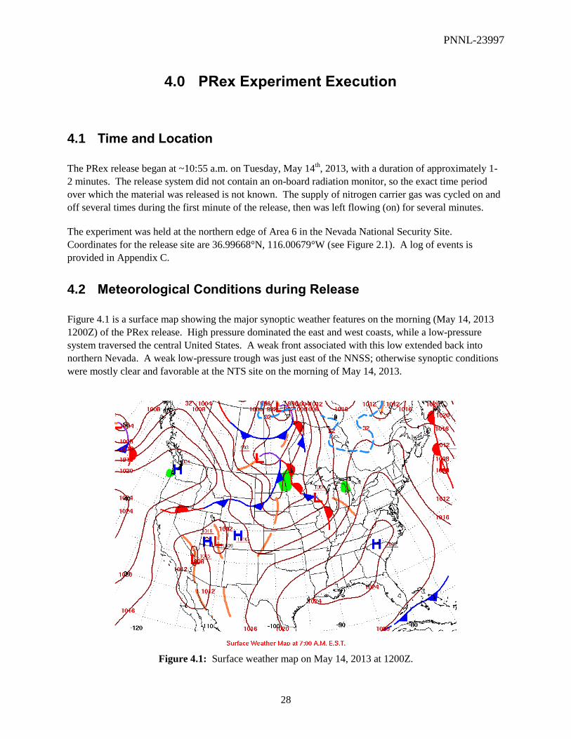
4.2 Meteorological Conditions during Release
Figure 4.1 is a surface map showing the major synoptic weather features on the morning (May 14, 2013
1200Z) of the PRex release. High pressure dominated the east and west coasts, while a low-pressure
system traversed the central United States. A weak front associated with this low extended back into
northern Nevada. A weak low-pressure trough was just east of the NNSS; otherwise synoptic conditions
were mostly clear and favorable at the NTS site on the morning of May 14, 2013.
Figure 4.1: Surface weather map on May 14, 2013 at 1200Z.

PNNL-23997
29
Figure 4.2 shows wind observations across the NTS site on May 14, 2013 10:45 a.m., approximately
10 minutes prior to the PRex release. Winds within the Yucca Flat basin were upslope, which is typical
for this area at this time of day in the absence of any large-scale weather systems. In Area 6, winds were
generally from the south at 10 mph, and became more south-southeasterly farther to the north (Areas 1, 4,
and 9). Table 4-1 shows the corresponding meteorological observations at the primary PRex
meteorological station (AP6) and nearby Meteorological data acquisition (MEDA) stations on May 14,
2013, 10:45 a.m.
Figure 4.2: Wind observations across the NTS site on May 14, 2013 10:45 a.m.
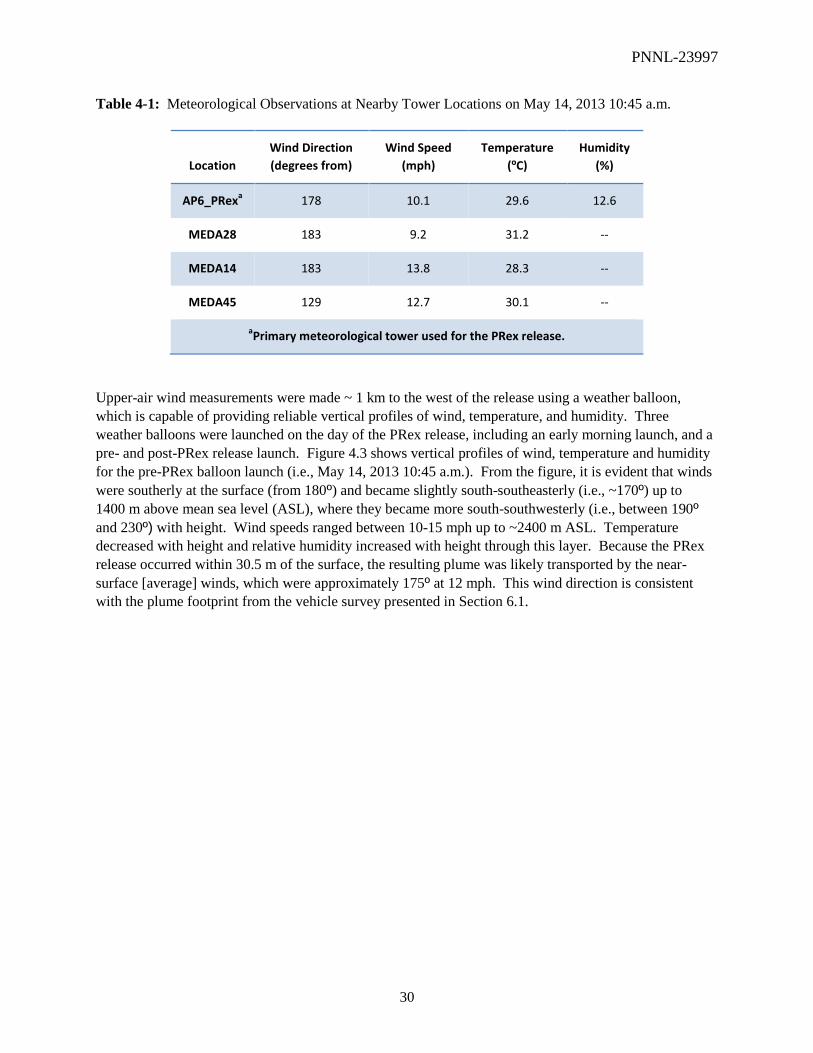
PNNL-23997
30
Table 4-1: Meteorological Observations at Nearby Tower Locations on May 14, 2013 10:45 a.m.
Location
Wind Direction
(degrees from)
Wind Speed
(mph)
Temperature
(ºC)
Humidity
(%)
AP6_PRexa
178 10.1 29.6 12.6
MEDA28 183 9.2 31.2 --
MEDA14 183 13.8 28.3 --
MEDA45 129 12.7 30.1 --
aPrimary meteorological tower used for the PRex release.
Upper-air wind measurements were made ~ 1 km to the west of the release using a weather balloon,
which is capable of providing reliable vertical profiles of wind, temperature, and humidity. Three
weather balloons were launched on the day of the PRex release, including an early morning launch, and a
pre- and post-PRex release launch. Figure 4.3 shows vertical profiles of wind, temperature and humidity
for the pre-PRex balloon launch (i.e., May 14, 2013 10:45 a.m.). From the figure, it is evident that winds
were southerly at the surface (from 180º) and became slightly south-southeasterly (i.e., ~170º) up to
1400 m above mean sea level (ASL), where they became more south-southwesterly (i.e., between 190º
and 230º) with height. Wind speeds ranged between 10-15 mph up to ~2400 m ASL. Temperature
decreased with height and relative humidity increased with height through this layer. Because the PRex
release occurred within 30.5 m of the surface, the resulting plume was likely transported by the near-
surface [average] winds, which were approximately 175º at 12 mph. This wind direction is consistent
with the plume footprint from the vehicle survey presented in Section 6.1.

PNNL-23997
31
Figure 4.3: Balloon profiles of wind, temperature, and humidity pre-PRex release (i.e., May 14, 2013
10:45 a.m.)
PNNL-23997
32
4.3 Sampling Network
4.3.1 Collection of Witness Plates
After an initial collection transit along the 1-km north row, when the plume location was still not fully
known, the witness plates in general were collected from north to south. This sequence reflected an effort
to avoid re-suspending particles in the more active regions so they would not be deposited onto
uncollected witness plates further north. The most active regions of the plume area were also off-limits
during the first day or so until the HCA staked out prior to the release was downgraded to a CA (except
for the area immediately around the release point, which remained off-limits for several weeks). Both
types of witness plates at a given location were collected at the same time and collection of all the sites
was accomplished over two days, Tuesday afternoon and Wednesday. It is important to point out that the
witness plates remained uncovered until they were collected, leaving open the possibility of additional
radiation and microsphere collections due to resuspension. Indeed, it was quite windy after the
experiment, with steady wind speeds in the vicinity of 10 m/s, and gusting to 15 m/s; dust devils were
also observed to transit the plume area over the coming days (including prior to collection of the witness
plates). The vehicles (pick-up truck or Kawasaki Mule) used to collect the witness plates could also
potentially cause resuspension, and to the extent possible were driven downwind (north) of the immediate
sampling locations.
The foam backing of each large witness plate was pre-scored so that the two halves could be folded
together easily after removal of the tent stakes holding each to the ground. Unfortunately, the halves did
not really adhere to each other as intended. During collection, the tacky mats were less sticky due to
collection of blowing dust / debris. Also, most of the foam boards had bowed while staked to the ground
(perhaps due to sun exposure), so that the two sides of the tacky mat did not come into close contact when
the foam boards were folded. Consistently strong and gusty winds were present during sample collection,
and it appeared that the daytime temperatures, winds, and personal protective equipment (PPE) would
introduce a risk of personnel overheating while working in the field with no shade. It was decided to
collect the samples quickly in the field, and to remove the tacky mats from their foam boards inside a
Conex container near the exit to the CA rather than out at the sampling sites. Each large witness plate
was folded and placed in its own plastic bag; these in turn were placed in a larger plastic bag in an effort
to limit cross contamination (primarily from the dust resuspended by the collection vehicle. Gloves were
also changed between samples. The high winds often made it difficult to place the witness plates into the
plastic bags, as did the bowed corners (see Figure 4.4).
After collection, the witness plate samples were returned to the Conex container for processing into
measurement geometry. The large area witness plate samples were processed on a table in the Conex;
each sample was removed and placed on top of its own plastic bag to minimize cross-contamination. All
of the tacky mat layers were removed from the foam and folded in a predetermined and consistent manner
to fit inside a new, sealable sample bag for counting on a high-purity germanium (HPGe) detector in the
Field Laboratory. The samples were folded into a square having area similar to the HPGe detector face,
so the sample bag could be laid flat on the detector face for counting. Although this process resulted in

PNNL-23997
33
extra unexposed tacky mat material being included in the sample, operationally it was easier to remove all
of the tacky-mat layers rather than just the top-most one.
Figure 4.4: Collection of tacky mat witness plate hampered by the bowed shape and the wind
The glass witness plates were collected by first placing a second glass plate on the sticky top of the
witness plate, sealing in the sampled dust and microspheres. The sandwiched sample was then removed
from the garden stake and placed in a sealed sample bag (also in the Conex container). The intent had
been that the tape holding the glass slide to the garden stake would be removed. However, while setting
up the sampling witness plates, the decision was made to use more robust duct tape rather than shipping
tape due to concerns about the wind. This duct tape, however, proved to be extremely difficult to remove
from the glass slides in the field without breaking them, and so was left on the glass witness plates.
4.3.2 Soil Sampling
In addition to the two types of witness plates, at several sampling sites, three different soil sampling
techniques were utilized during the PRex experiment. The principle motivator of this was that the three
techniques were under consideration by the CTBTO for soil sampling during an OSI. While the above-
mentioned witness plates are ideal for pre-planned characterization of a release event, soil sampling is an
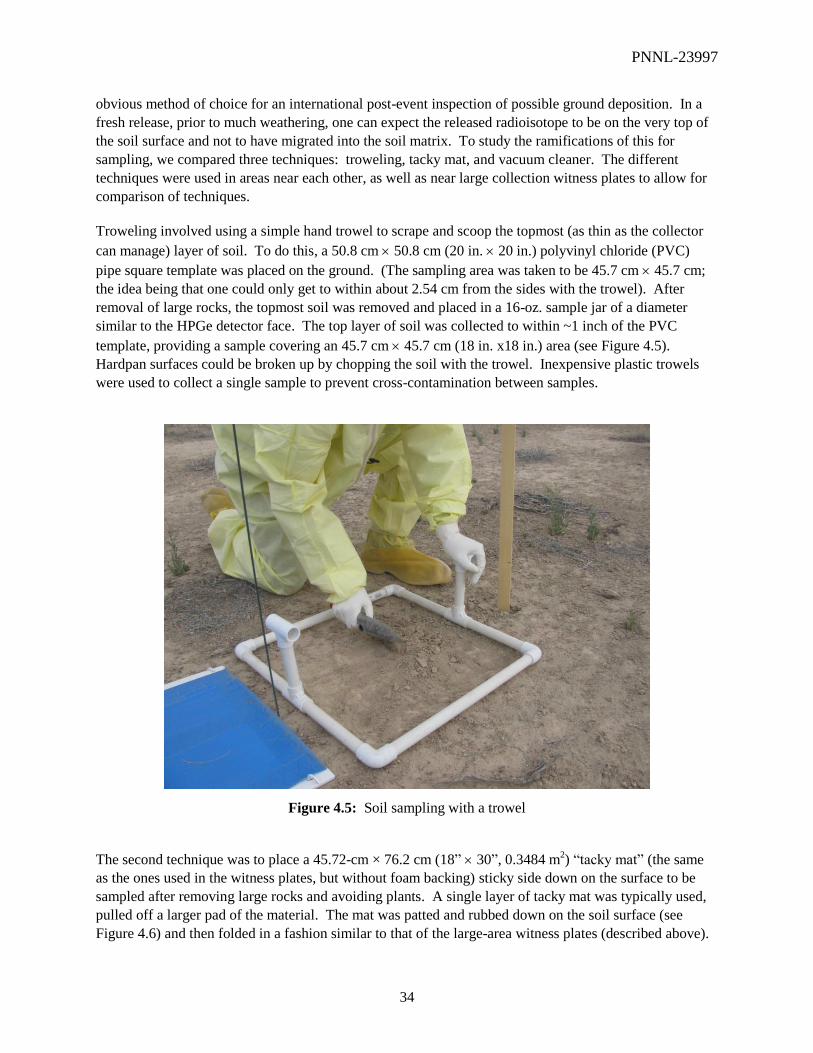
PNNL-23997
34
obvious method of choice for an international post-event inspection of possible ground deposition. In a
fresh release, prior to much weathering, one can expect the released radioisotope to be on the very top of
the soil surface and not to have migrated into the soil matrix. To study the ramifications of this for
sampling, we compared three techniques: troweling, tacky mat, and vacuum cleaner. The different
techniques were used in areas near each other, as well as near large collection witness plates to allow for
comparison of techniques.
Troweling involved using a simple hand trowel to scrape and scoop the topmost (as thin as the collector
can manage) layer of soil. To do this, a 50.8 cm 50.8 cm (20 in. 20 in.) polyvinyl chloride (PVC)
pipe square template was placed on the ground. (The sampling area was taken to be 45.7 cm 45.7 cm;
the idea being that one could only get to within about 2.54 cm from the sides with the trowel). After
removal of large rocks, the topmost soil was removed and placed in a 16-oz. sample jar of a diameter
similar to the HPGe detector face. The top layer of soil was collected to within ~1 inch of the PVC
template, providing a sample covering an 45.7 cm 45.7 cm (18 in. x18 in.) area (see Figure 4.5).
Hardpan surfaces could be broken up by chopping the soil with the trowel. Inexpensive plastic trowels
were used to collect a single sample to prevent cross-contamination between samples.
Figure 4.5: Soil sampling with a trowel
The second technique was to place a 45.72-cm × 76.2 cm (18” 30”, 0.3484 m2) “tacky mat” (the same
as the ones used in the witness plates, but without foam backing) sticky side down on the surface to be
sampled after removing large rocks and avoiding plants. A single layer of tacky mat was typically used,
pulled off a larger pad of the material. The mat was patted and rubbed down on the soil surface (see
Figure 4.6) and then folded in a fashion similar to that of the large-area witness plates (described above).

PNNL-23997
35
Due to the large number of very small pebbles typically collected by this method, these folded mats
would not fit into plastic bags like the witness plate samples, so they were placed in sample jars like those
used for the troweled samples.
Figure 4.6: Soil sampling with a tacky mat
The third technique involved the use of a handheld vacuum cleaner (colloquially known in the U.S. as a
“Dust Buster,” though in this case we actually used a Dirt Devil brand Handy Duo.) These units are
battery powered, though we soon observed that they do not actually last very long on battery power
before needing to be recharged. For this technique, we used the same square PVC template as was used
for troweling. To prevent coarse material from reaching the finer filters we improvised a filter by
inserting a knee-high panty hose into the vacuum cleaner and holding it around the mouth of the vacuum
cleaner while the panty hose toe was sucked inside. (No vacuum cleaner attachments were used.) The
vacuum cleaner was then moved back and forth over the soil surface as close as possible (see Figure 4.7).
In areas where the soil was loose enough to be sucked up en masse, it was necessary to keep the vacuum
cleaner off of the surface a bit, but otherwise, it could go along the surface. As in the tacky mat case, the
numerous small pebbles typically present were a challenge for this technique. The entire surface area was
usually vacuumed twice. Next the vacuum cleaner was disassembled over a sample jar like those used for
the previous techniques. The panty hose and the coarse material inside were placed in the sample jar,
along with the material in front of the vacuum cleaner’s filter. This filter was removed and shaken into
the jar, along with the finer material between it and a second filter. The outer vacuum cleaner tube and
initial collection area could be mostly wiped down with wet wipes between samples, but this was not true
for the inner filters, which trapped moisture in their filter pores. Thus this technique is more susceptible
to cross-contamination in addition to its logistical difficulties relative to the other two soil sampling
techniques.

PNNL-23997
36
Figure 4.7: Soil sampling with battery-powered vacuum cleaner
4.3.3 Air Sampling
The gasoline-powered high-volume samplers placed km downwind of the dispersal were started at
approximately 9:30 a.m. and allowed to run until the filter samples were collected between 3 p.m. and 4
p.m. The battery-powered high-volume samplers at 1.5 km downwind were remotely started a few
minutes before the source release, and allowed to run for 20 minutes. Filter paper samples from both the
gasoline- and battery-powered samplers were collected between 3 p.m. and 4 p.m. The PAPR samplers
were started between 9 a.m. and 10 a.m., and allowed to run until their batteries were exhausted
(approximately 10 hours).
The gasoline-powered high-volume air samplers were restarted at 10 a.m. on May 15th to look for
resuspension of 140
La kicked up by survey activities and the afternoon winds.
4.4 Radiation Survey
High (HPGe), medium (LaBr3 and NaI) and low (polyvinyl toluene (PVT)—used as gross count) energy
resolution capable instrumentation was brought to NNSS by PNNL to enable comparison between these
instruments’ capabilities to characterize a potential release from a nuclear weapons test of interest for an
OSI under CTBT.
In addition to work performed with PNNL-owned instruments, Remote Sensing Laboratory (RSL)
performed a flight with their fixed-wing aircraft on the day of the release. The surveys are discussed in
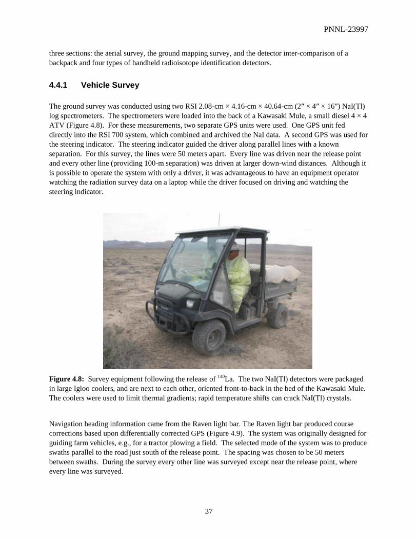
PNNL-23997
37
three sections: the aerial survey, the ground mapping survey, and the detector inter-comparison of a
backpack and four types of handheld radioisotope identification detectors.
4.4.1 Vehicle Survey
The ground survey was conducted using two RSI 2.08-cm × 4.16-cm × 40.64-cm (2″ × 4″ × 16″) NaI(Tl)
log spectrometers. The spectrometers were loaded into the back of a Kawasaki Mule, a small diesel 4 × 4
ATV (Figure 4.8). For these measurements, two separate GPS units were used. One GPS unit fed
directly into the RSI 700 system, which combined and archived the NaI data. A second GPS was used for
the steering indicator. The steering indicator guided the driver along parallel lines with a known
separation. For this survey, the lines were 50 meters apart. Every line was driven near the release point
and every other line (providing 100-m separation) was driven at larger down-wind distances. Although it
is possible to operate the system with only a driver, it was advantageous to have an equipment operator
watching the radiation survey data on a laptop while the driver focused on driving and watching the
steering indicator.
Figure 4.8: Survey equipment following the release of 140
La. The two NaI(Tl) detectors were packaged
in large Igloo coolers, and are next to each other, oriented front-to-back in the bed of the Kawasaki Mule.
The coolers were used to limit thermal gradients; rapid temperature shifts can crack NaI(Tl) crystals.
Navigation heading information came from the Raven light bar. The Raven light bar produced course
corrections based upon differentially corrected GPS (Figure 4.9). The system was originally designed for
guiding farm vehicles, e.g., for a tractor plowing a field. The selected mode of the system was to produce
swaths parallel to the road just south of the release point. The spacing was chosen to be 50 meters
between swaths. During the survey every other line was surveyed except near the release point, where
every line was surveyed.
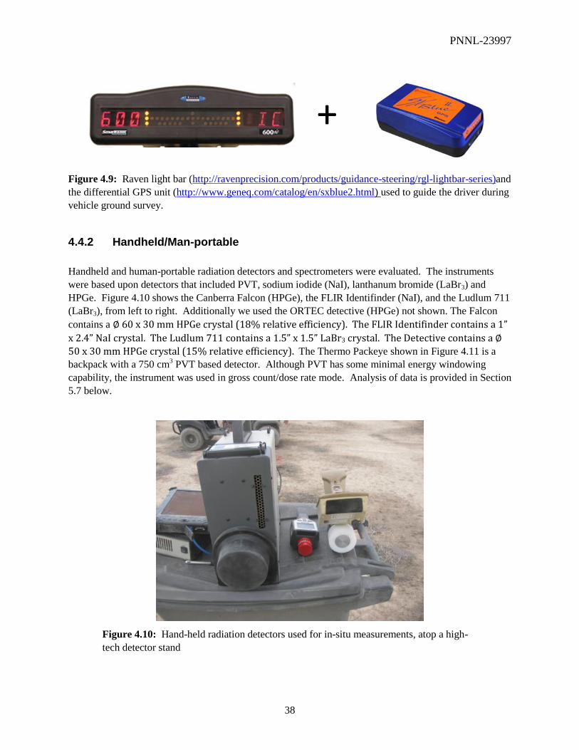
PNNL-23997
38
Figure 4.9: Raven light bar (http://ravenprecision.com/products/guidance-steering/rgl-lightbar-series)and
the differential GPS unit (http://www.geneq.com/catalog/en/sxblue2.html) used to guide the driver during
vehicle ground survey.
4.4.2 Handheld/Man-portable
Handheld and human-portable radiation detectors and spectrometers were evaluated. The instruments
were based upon detectors that included PVT, sodium iodide (NaI), lanthanum bromide (LaBr3) and
HPGe. Figure 4.10 shows the Canberra Falcon (HPGe), the FLIR Identifinder (NaI), and the Ludlum 711
(LaBr3), from left to right. Additionally we used the ORTEC detective (HPGe) not shown. The Falcon
contains a ∅ 60 x 30 mm HPGe crystal (18% relative efficiency). The FLIR Identifinder contains a 1”
x 2.4” NaI crystal. The Ludlum 711 contains a 1.5” x 1.5” LaBr3 crystal. The Detective contains a ∅
50 x 30 mm HPGe crystal (15% relative efficiency). The Thermo Packeye shown in Figure 4.11 is a
backpack with a 750 cm3 PVT based detector. Although PVT has some minimal energy windowing
capability, the instrument was used in gross count/dose rate mode. Analysis of data is provided in Section
5.7 below.
Figure 4.10: Hand-held radiation detectors used for in-situ measurements, atop a high-
tech detector stand
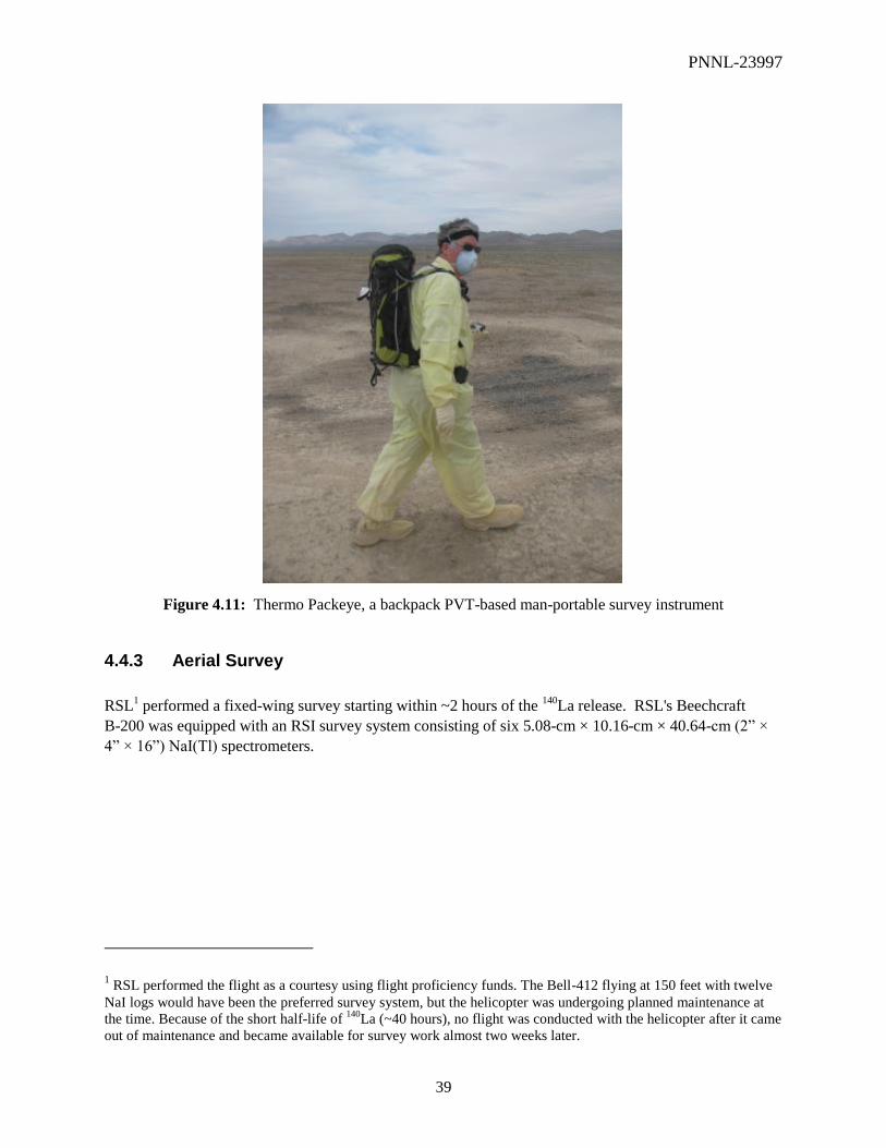
PNNL-23997
39
Figure 4.11: Thermo Packeye, a backpack PVT-based man-portable survey instrument
4.4.3 Aerial Survey
RSL1 performed a fixed-wing survey starting within ~2 hours of the
140La release. RSL's Beechcraft
B-200 was equipped with an RSI survey system consisting of six 5.08-cm × 10.16-cm × 40.64-cm (2” ×
4” × 16”) NaI(Tl) spectrometers.
1 RSL performed the flight as a courtesy using flight proficiency funds. The Bell-412 flying at 150 feet with twelve
NaI logs would have been the preferred survey system, but the helicopter was undergoing planned maintenance at
the time. Because of the short half-life of 140
La (~40 hours), no flight was conducted with the helicopter after it came
out of maintenance and became available for survey work almost two weeks later.

PNNL-23997
40
Flight lines were flown 500 feet above ground level (AGL) at a speed of 140 knots at a line spacing of
500 feet. Images of the B-200 taken while performing the aerial survey following the 140
La release and
from the NNSA website are shown in Figure 4.12.
Figure 4.12: B-200 performing aerial survey of 140
La release (left) and image of aircraft from an AMS
presentation (right) (Lyons 2012)
4.5 Field Laboratory
A field laboratory was set up in a Quonset hut several miles to the southwest of the release point, in
the “Command Post” area of the test site (see Figure 4.13). The laboratory included three ~50% relative
efficiency high resolution germanium HPGe gamma spectrometers (Canberra), as well as two low
resolution 7.62 cm × 12.7 cm (3” × 5”) NaI(Tl) spectrometers. The lab was manned by two to three
personnel throughout the duration of sample measurements, and depended upon personnel availability.

PNNL-23997
41
Figure 4.13: Exterior of Quonset hut that housed the field laboratory for PRex. Note the liquid nitrogen
dewars provided for cooling of the HPGe detectors, on right.
Straight-forward 10.16 cm (4”) thick lead shields were built on stands to accommodate two of the HPGe
detectors (see Figure 4.14) and the two NaI(Tl) detectors (Figure 4.15). The third HPGe detector, supplied
by NSTec, was housed in a Canberra portable shield (Figure 4.16). This detector was calibrated on the
Canberra ISOCS system, and models were developed to establish detection efficiencies for the sample
geometries during build up and preparation of the laboratory. Efficiency calibrations were also estimated
for the PNNL-supplied HPGe detectors using the ISOCS methods.
Figure 4.14: Two ~50% relative efficiency HPGe detectors inside of 10.16 cm (4”) thick lead shields.
These detectors are set up in the field laboratory.

PNNL-23997
42
Figure 4.15: Single shield housing two 7.62 cm × 12.7 cm (3” × 5”) NaI(Tl) detectors. The detectors are
surrounded by 10.16 cm (4”) of lead, and the sample chambers are also separated by 10.16 cm (4”) of
lead.
Figure 4.16: Canberra HPGe with commercial portable shield system, supplied by NSTec. The Canberra
ISOCs efficiency calibration on this system was used to cross-calibrate the other HPGe detectors.
The first samples received into the field laboratory were collected by the high volume air samplers 2 km
downwind from the release, and were brought to the laboratory late in the day on Tuesday, May 14th. A
large fraction of the samples were received into the lab on Wednesday, with additional samples received
Thursday morning. Counting was performed beginning late Tuesday, and was completed Friday morning,

PNNL-23997
43
followed by tear-down and loading of the laboratory late Friday morning. Table A-1 provides the number
of sample measurements performed. Samples were typically counted for 15 minutes; samples that had
weak positive indications for 140
La were extended to 30 minutes of counting to improve the result.
The two NaI(Tl) detectors were included in the field laboratory because they were expected to be more
reliable than the HPGe detectors; the utility and sensitivity of the NaI(Tl) detectors was unclear. Early
sample measurements made it clear that the NaI(Tl) sensitivity was far inferior to that of the HPGe
detectors due to the significant background rates relative to the 140
La activity (in the NaI(Tl) spectra,
natural 40
K was a significant interference for the 1596 keV 140
La line). One of the NaI(Tl) detectors also
suffered from degraded energy resolution, and was essentially un-useable. After early attempts to use the
NaI(Tl) detectors in a screening mode, they were no longer used as they were not providing added-value.
It seems likely that scintillators, with their poorer energy resolution compared to HPGe, would likely
require a high efficiency coincidence configuration to provide added value.

PNNL-23997
44
5.0 Analysis of Results
5.1 Vehicle Survey
The mobile survey of the PRex release area was performed over two days, May 15 and May 16, roughly
during the time windows 21-29 hours and 45-53 hours after the release. The survey was performed with a
two NaI (Tl) log RSI system located in the cargo space of a Kawasaki Mule. The survey lines were driven
in the East and West directions and were typically 100 meters apart. The survey started at the original
northern border of the HCA (~ 0.5 km north of the release point) and moved northwards. During the
morning of the 15th, the survey was performed solely by an equipment operator also acting as the driver.
In the afternoon and following day, a driver from NSTec drove the vehicle freeing the PNNL operator to
focus on data collection. The survey data set suffered from some data drop out periods (mainly in one
detector, although in some cases data acquisition for both detectors stopped for brief periods), and from
problems with the automated energy calibration function erroneously identifying the 1596 keV 140
La line
as the 40
K 1461 keV line. Data corrections were applied, and are described in detail in Appendix A.
Figure 5.1shows a survey plot typical of the products generated after data corrections were applied; in this
case, detector count rates in a region of interest (ROI) around the 1596-keV gamma energy of 140
La are
shown.
NSTec reduced the HCA restriction down to the ~ 20 meter × 20 meter fence surrounding the release
point based upon “stomp and tromp” surveys during the afternoon of the 15. On May 16, the vehicle
survey team filled in lines starting at the previous HCA northern border and measured lines south
extending beyond the point of release. In this southern region of the survey, the spacing between survey
lines was reduced to 50 meters to provide more detail to the close-in survey data.
On May 16, the team also surveyed the lines extending northward of where the survey had reached on the
15. The northern-most survey line was 2 km north of the release point. A combined path plot of the
survey conducted on the 15 and 16 is shown in Figure 5.2. The path plot is based upon the gross counts
of the spectral data; i.e., it is a plot of the physical position for each 1 second measurement, colorized to
reflect the sum of counts (in both detectors) over the full spectrum. The energy range is ~50 to 3000 keV.
In this figure the color break points were chosen to emphasize the location of plume and the level of the
background with a minimal set of colors. The breakpoints are at 5000, 5500, 6000 and 6500 cps.
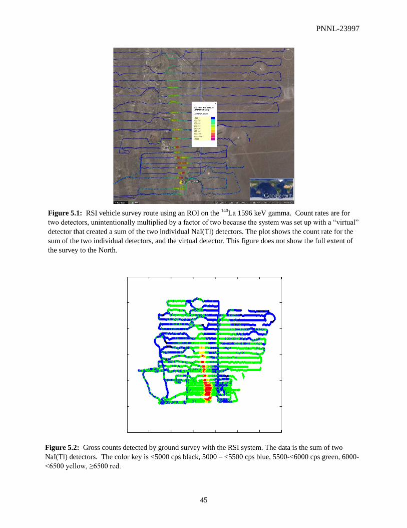
PNNL-23997
45
Figure 5.1: RSI vehicle survey route using an ROI on the 140
La 1596 keV gamma. Count rates are for
two detectors, unintentionally multiplied by a factor of two because the system was set up with a “virtual”
detector that created a sum of the two individual NaI(Tl) detectors. The plot shows the count rate for the
sum of the two individual detectors, and the virtual detector. This figure does not show the full extent of
the survey to the North.
Figure 5.2: Gross counts detected by ground survey with the RSI system. The data is the sum of two
NaI(Tl) detectors. The color key is <5000 cps black, 5000 – <5500 cps blue, 5500-<6000 cps green, 6000-
<6500 yellow, ≥6500 red.
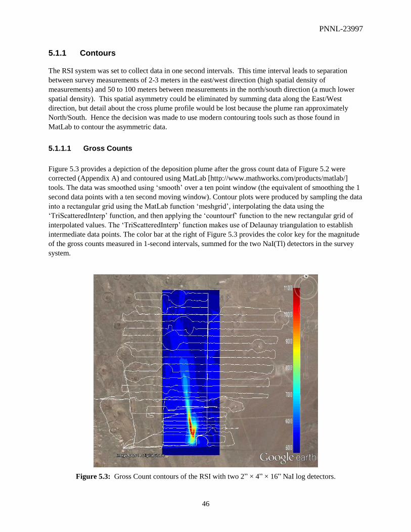
PNNL-23997
46
5.1.1 Contours
The RSI system was set to collect data in one second intervals. This time interval leads to separation
between survey measurements of 2-3 meters in the east/west direction (high spatial density of
measurements) and 50 to 100 meters between measurements in the north/south direction (a much lower
spatial density). This spatial asymmetry could be eliminated by summing data along the East/West
direction, but detail about the cross plume profile would be lost because the plume ran approximately
North/South. Hence the decision was made to use modern contouring tools such as those found in
MatLab to contour the asymmetric data.
5.1.1.1 Gross Counts
Figure 5.3 provides a depiction of the deposition plume after the gross count data of Figure 5.2 were
corrected (Appendix A) and contoured using MatLab [http://www.mathworks.com/products/matlab/]
tools. The data was smoothed using ‘smooth’ over a ten point window (the equivalent of smoothing the 1
second data points with a ten second moving window). Contour plots were produced by sampling the data
into a rectangular grid using the MatLab function ‘meshgrid’, interpolating the data using the
‘TriScatteredInterp’ function, and then applying the ‘countourf’ function to the new rectangular grid of
interpolated values. The ‘TriScatteredInterp’ function makes use of Delaunay triangulation to establish
intermediate data points. The color bar at the right of Figure 5.3 provides the color key for the magnitude
of the gross counts measured in 1-second intervals, summed for the two NaI(Tl) detectors in the survey
system.
Figure 5.3: Gross Count contours of the RSI with two 2” × 4” × 16” NaI log detectors.
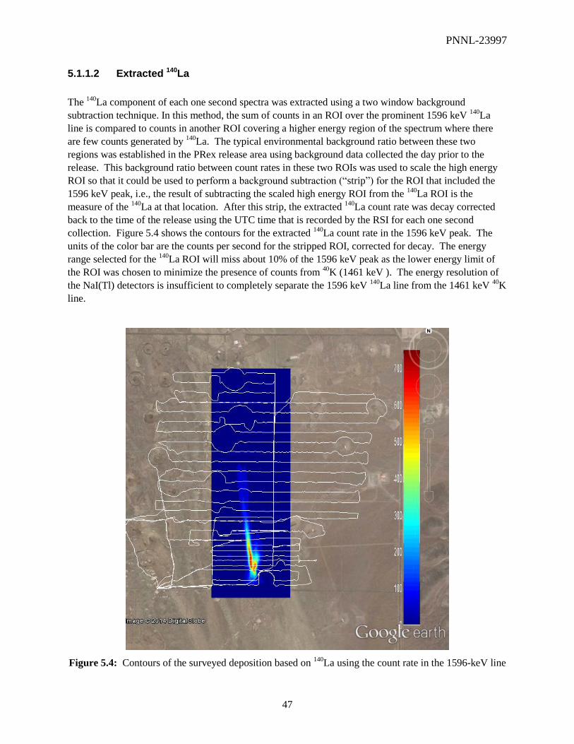
PNNL-23997
47
5.1.1.2 Extracted 140La
The 140
La component of each one second spectra was extracted using a two window background
subtraction technique. In this method, the sum of counts in an ROI over the prominent 1596 keV 140
La
line is compared to counts in another ROI covering a higher energy region of the spectrum where there
are few counts generated by 140
La. The typical environmental background ratio between these two
regions was established in the PRex release area using background data collected the day prior to the
release. This background ratio between count rates in these two ROIs was used to scale the high energy
ROI so that it could be used to perform a background subtraction (“strip”) for the ROI that included the
1596 keV peak, i.e., the result of subtracting the scaled high energy ROI from the 140
La ROI is the
measure of the 140
La at that location. After this strip, the extracted 140
La count rate was decay corrected
back to the time of the release using the UTC time that is recorded by the RSI for each one second
collection. Figure 5.4 shows the contours for the extracted 140
La count rate in the 1596 keV peak. The
units of the color bar are the counts per second for the stripped ROI, corrected for decay. The energy
range selected for the 140
La ROI will miss about 10% of the 1596 keV peak as the lower energy limit of
the ROI was chosen to minimize the presence of counts from 40
K (1461 keV ). The energy resolution of
the NaI(Tl) detectors is insufficient to completely separate the 1596 keV 140
La line from the 1461 keV 40
K
line.
Figure 5.4: Contours of the surveyed deposition based on 140
La using the count rate in the 1596-keV line
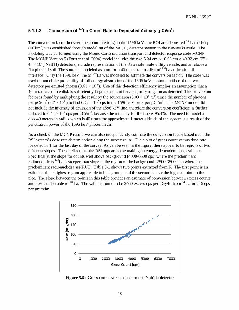
PNNL-23997
48
5.1.1.3 Conversion of 140La Count Rate to Deposited Activity (μCi/m2)
The conversion factor between the count rate (cps) in the 1596 keV line ROI and deposited 140
La activity
(μCi/m2) was established through modeling of the NaI(Tl) detector system in the Kawasaki Mule. The
modeling was performed using the Monte Carlo radiation transport and detector response code MCNP.
The MCNP Version 5 (Forster et al. 2004) model includes the two 5.04 cm × 10.08 cm × 40.32 cm (2” ×
4” × 16”) NaI(Tl) detectors, a crude representation of the Kawasaki mule utility vehicle, and air above a
flat plane of soil. The source is modeled as a uniform 40 meter radius disk of 140
La at the air-soil
interface. Only the 1596 keV line of 140
La was modeled to estimate the conversion factor. The code was
used to model the probability of full energy absorption of the 1596 keV photon in either of the two
detectors per emitted photon (3.61 × 10⁻⁶
). Use of this detection efficiency implies an assumption that a
40 m radius source disk is sufficiently large to account for a majority of gammas detected. The conversion
factor is found by multiplying the result by the source area (5.03 × 10³ m
2)
times the number of photons
per μCi/m2 (3.7 × 10
4 ) to find 6.72 × 10
2 cps in the 1596 keV peak per μCi/m
2. The MCNP model did
not include the intensity of emission of the 1596 keV line, therefore the conversion coefficient is further
reduced to 6.41 × 10² cps per μCi/m
2, because the intensity for the line is 95.4%. The need to model a
disk 40 meters in radius which is 40 times the approximate 1 meter altitude of the system is a result of the
penetration power of the 1596 keV photon in air.
As a check on the MCNP result, we can also independently estimate the conversion factor based upon the
RSI system’s dose rate determination along the survey route. F is a plot of gross count versus dose rate
for detector 1 for the last day of the survey. As can be seen in the figure, there appear to be regions of two
different slopes. These reflect that the RSI appears to be making an energy dependent dose estimate.
Specifically, the slope for counts well above background (4000-6500 cps) where the predominant
radionuclide is 140
La is steeper than slope in the region of the background (2500-3500 cps) where the
predominant radionuclides are KUT. Table 5-1 shows two points extracted from F. The first point is an
estimate of the highest region applicable to background and the second is near the highest point on the
plot. The slope between the points in this table provides an estimate of conversion between excess counts
and dose attributable to 140
La. The value is found to be 2460 excess cps per nGy/hr from 140
La or 246 cps
per μrem/hr.
Figure 5.5: Gross counts versus dose for one NaI(Tl) detector
0
50
100
150
200
250
0 1000 2000 3000 4000 5000 6000 7000
Do
se (
nG
y/h
r)
Gross Count (cps)

PNNL-23997
49
Table 5-1: Typical Values Extracted from Figure 6-3
CPS nGy/hr Comment
3728 101.7 Estimated highest background
6232 203.7 Highest value (background + 140
La)
From Table 5-1, the conversion coefficient for 140
La gross counts is (6232-3728)/((203.7-101.7)/10) or
245.5 cps per μrem/hr (the conversion factor between nGy/hr and μrem/hr is approximately 1/10). From
the Nuclear Regulatory Commission’s RadToolbox [NRC 2014], an infinite plane source of 140
La with an
activity of 1 μCi/m2 produces a dose at 1 m elevation of 28.8 μrem/hr. Hence, according to this estimate, a
single 2” × 4” × 16” NaI(Tl) detector should produce 7070 cps (gross counts) per μCi/m2 of
140La.
However, these are gross counts rather than counts in the ROI around 1596 keV . To understand the ratio
of counts from 140
La in the gross count to those in the ROI, it was necessary to compare spectra with and
without 140
La. Two seventeen second spectra were compared. In Table 5-2, the data without 140
La,
labeled “Background”, came from a survey conducted in the PRex release area on May 13 which was the
day before the release. The data labeled “With 140
La” was measured on the morning of May 15.
Table 5-2: Comparison of ROI and GC Counts in Spectra with and without 140
La
Start time index Stop time index ROI counts Gross Count
With 140La 2640 2668 2436 199102
Background 400 428 391 157819
Net 2045 41283
The ratio of 140
La in the full spectrum (gross count) to 140
La in the ROI is ~20. Therefore, the expected
excess counts in one NaI(Tl) detector is 7070/20, or ~353 cps per μCi/m2 of
140La. This rough estimate
compares well (~10%) with the value based upon the MCNP modeled conversion of 321 cps/(μCi/m2) for
a single RSI NaI(Tl) detector.
Returning to the MCNP-derived conversion factor of 641 cps/(μCi/m2) for two RSI NaI(Tl) detectors, it
becomes possible to convert interpolated data points to a uniform grid of deposited activity values and to
integrate the result to estimate the quantity of 140
La deposited in the observable plume. This integration
of the plume results in an estimate that the measured 140
La is of the order of 7% of the original ~1 Ci
quantity available for release. This result may reflect that the release was not fully successful (source
material left in or around the transport container), or that we did not have a full understanding of the
source particle size. Analyses of the particle distribution in the released powder that were completed after
the release indicated a range of particles extending into smaller particles than intended; this would result
in longer distance transport and less activity deposition in the near field.
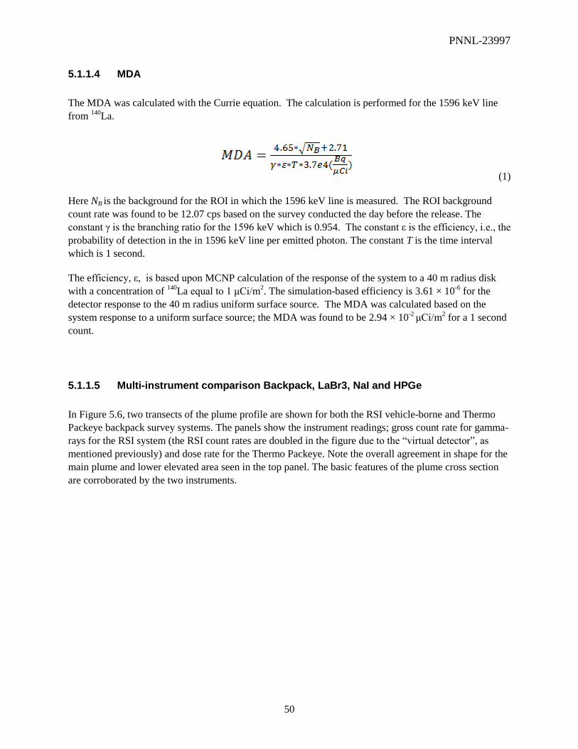
PNNL-23997
50
5.1.1.4 MDA
The MDA was calculated with the Currie equation. The calculation is performed for the 1596 keV line
from 140
La.
(1)
Here NB is the background for the ROI in which the 1596 keV line is measured. The ROI background
count rate was found to be 12.07 cps based on the survey conducted the day before the release. The
constant γ is the branching ratio for the 1596 keV which is 0.954. The constant ε is the efficiency, i.e., the
probability of detection in the in 1596 keV line per emitted photon. The constant T is the time interval
which is 1 second.
The efficiency, ε, is based upon MCNP calculation of the response of the system to a 40 m radius disk
with a concentration of 140
La equal to 1 μCi/m2. The simulation-based efficiency is 3.61 × 10
-6 for the
detector response to the 40 m radius uniform surface source. The MDA was calculated based on the
system response to a uniform surface source; the MDA was found to be 2.94 × 10⁻²
μCi/m2 for a 1 second
count.
5.1.1.5 Multi-instrument comparison Backpack, LaBr3, NaI and HPGe
In Figure 5.6, two transects of the plume profile are shown for both the RSI vehicle-borne and Thermo
Packeye backpack survey systems. The panels show the instrument readings; gross count rate for gamma-
rays for the RSI system (the RSI count rates are doubled in the figure due to the “virtual detector”, as
mentioned previously) and dose rate for the Thermo Packeye. Note the overall agreement in shape for the
main plume and lower elevated area seen in the top panel. The basic features of the plume cross section
are corroborated by the two instruments.

PNNL-23997
51
Figure 5.6: Comparison of vehicle and backpack transects of plume. The top (near sample area 1-4) and
bottom panel (near sample area 5-4) compare gross count (RSI) (RSI count rates are doubled due to
“virtual detector”) with dose rate (Packeye). The paths followed for the Packeye and RSI surveys were
close, but not precisely the same.
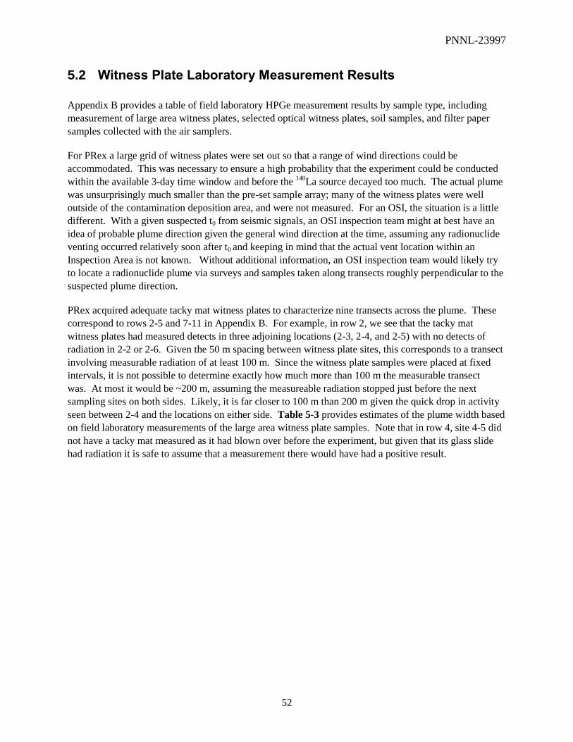
PNNL-23997
52
5.2 Witness Plate Laboratory Measurement Results
Appendix B provides a table of field laboratory HPGe measurement results by sample type, including
measurement of large area witness plates, selected optical witness plates, soil samples, and filter paper
samples collected with the air samplers.
For PRex a large grid of witness plates were set out so that a range of wind directions could be
accommodated. This was necessary to ensure a high probability that the experiment could be conducted
within the available 3-day time window and before the 140
La source decayed too much. The actual plume
was unsurprisingly much smaller than the pre-set sample array; many of the witness plates were well
outside of the contamination deposition area, and were not measured. For an OSI, the situation is a little
different. With a given suspected t0 from seismic signals, an OSI inspection team might at best have an
idea of probable plume direction given the general wind direction at the time, assuming any radionuclide
venting occurred relatively soon after t0 and keeping in mind that the actual vent location within an
Inspection Area is not known. Without additional information, an OSI inspection team would likely try
to locate a radionuclide plume via surveys and samples taken along transects roughly perpendicular to the
suspected plume direction.
PRex acquired adequate tacky mat witness plates to characterize nine transects across the plume. These
correspond to rows 2-5 and 7-11 in Appendix B. For example, in row 2, we see that the tacky mat
witness plates had measured detects in three adjoining locations (2-3, 2-4, and 2-5) with no detects of
radiation in 2-2 or 2-6. Given the 50 m spacing between witness plate sites, this corresponds to a transect
involving measurable radiation of at least 100 m. Since the witness plate samples were placed at fixed
intervals, it is not possible to determine exactly how much more than 100 m the measurable transect
was. At most it would be ~200 m, assuming the measureable radiation stopped just before the next
sampling sites on both sides. Likely, it is far closer to 100 m than 200 m given the quick drop in activity
seen between 2-4 and the locations on either side. Table 5-3 provides estimates of the plume width based
on field laboratory measurements of the large area witness plate samples. Note that in row 4, site 4-5 did
not have a tacky mat measured as it had blown over before the experiment, but given that its glass slide
had radiation it is safe to assume that a measurement there would have had a positive result.

PNNL-23997
53
Table 5-3: Deposition Plume Width Estimate Based on Large Area Witness Plates
Row Approximate plume width (m)
Based on witness plate measurements
2 100-200
3 150-250
4 200-300
5 200-400
7 100-300
8 300-500
9 200-400
10 200-400
11 600-800
Insufficient measurements of the large area witness plates in row 6 were made to characterize that transect
of the plume. This indicates that these samples were either not collected, were not processed correctly
(e.g. the wrong decision was made on whether to measure the sample), or the measurement data was lost.
In any event, this represents lost data that was intended to be available for the analysis. This is a situation
that can arise during the hectic pace of work that occurred after the dispersal, and is an issue that is likely
to be faced by OSI teams.
The conclusion is that for this plume and this level of activity, a sample spacing of much more than 100 m
would have possibly missed the plume. Given the winds at the time, this might be narrower than a typical
plume, but gives some idea of the challenge for an OSI team. Another thing worth pointing out about the
plume for consideration is that adjoining measured activities along a given transect (as shown in
Appendix B) typically differ by at least an order of magnitude.

PNNL-23997
54
5.3 Comparison of Vehicle Survey and Witness Plate Results
The surface area and measured activity of the tacky mats was used to determine the deposited activity in
μCi/m2. The equivalent RSI measurements are based upon the interpolation of the survey data to the
location of the tacky mats. The results have been corrected to a consistent set of units (Ci/m2), however
the tacky mat results represent a measurement of deposition on a 0.3484 m2 surface area, while the
MCNP detection efficiency calculations indicate that the RSI survey system is sensitive to large distances;
this was demonstrated by a significant change in the count rate conversion factor (see section 5.1.1.3)
when the MCNP modeled source disk was expanded from a ten meter radius to a forty meter radius. The
deposited plume activity concentration derived from field laboratory measurement of witness plates is
compared to the vehicle survey result for various witness plate locations as shown in Table 5-4 and
graphically in Figure 5.7. In the figure, the tacky mat results are shown as filled circles where the
coloring break points have been chosen to approximately match the colors on the contoured mobile data.
The mobile data is in cps for the ROI region. The conversion factor for the survey data is 641 cps per
μCi/m2, as discussed above. All are in good agreement except for 7-3, as discussed in the next section.
Table 5-4: Comparison of Tacky Mats and Mobile Survey
Location
Tacky Mats
(μCi/m2)
RSI
(μCi/m2)
2-4 0.53 0.78
5-4 0.092-0.12 0.10
7-3 0.00051 – 0.0032 0.18
10-5 0.05 – 0.057 0.06
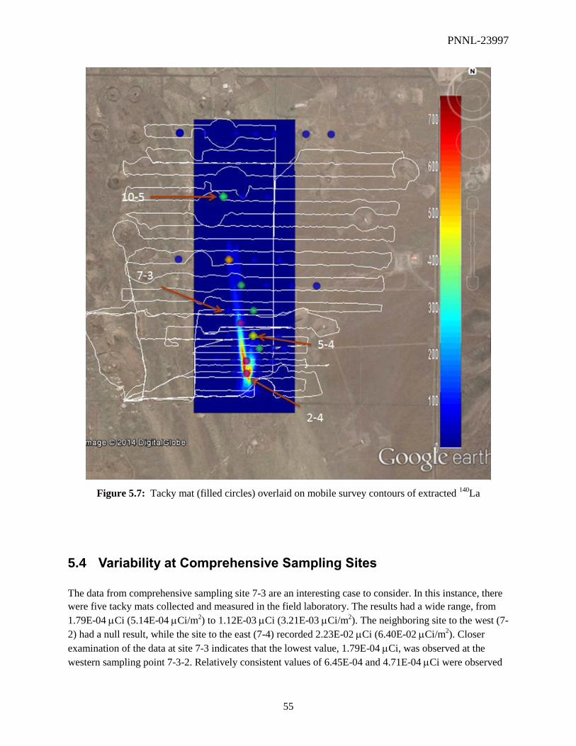
PNNL-23997
55
Figure 5.7: Tacky mat (filled circles) overlaid on mobile survey contours of extracted 140
La
5.4 Variability at Comprehensive Sampling Sites
The data from comprehensive sampling site 7-3 are an interesting case to consider. In this instance, there
were five tacky mats collected and measured in the field laboratory. The results had a wide range, from
1.79E-04 Ci (5.14E-04 Ci/m2) to 1.12E-03 Ci (3.21E-03Ci/m
2). The neighboring site to the west (7-
2) had a null result, while the site to the east (7-4) recorded 2.23E-02 Ci (6.40E-02 Ci/m2). Closer
examination of the data at site 7-3 indicates that the lowest value, 1.79E-04 Ci, was observed at the
western sampling point 7-3-2. Relatively consistent values of 6.45E-04and 4.71E-04 Ci were observed
PNNL-23997
56
at the center and southern sampling points, respectively. Finally, values of 9.33E-04 and 1.12E-03Ci
were observed at the northern and eastern points. While not conclusive, these results are consistent with a
factor of 6 increase in 140
La deposition over the scale of a comprehensive sampling site, ~6 meters.
Inspection of Figure 5.7 shows that this sampling site was likely in a location where there would be a
steep upward gradient of the plume when moving from west to east. The corresponding RSI vehicle
survey result was 1.8E-01 Ci/m2, significantly higher than results from the tacky mats. This could
indicate that the survey value was biased higher due to the higher activity nearby to the east.
Aside from the variation in witness plate results at sampling site 7-3, the results from the RSI vehicle
survey and the witness plate samples are in good agreement, as seen in Table 5-4. Two more of these
sampling locations were also comprehensive sampling sites, 5-4 and 10-5. Both of these sites displayed
good agreement among the five tacky mat samples collected at each site. The activity levels at both sites
were higher than at 7-3. Neither of these sites appears to lie on a steep activity gradient (see Figure 5.7),
so the good agreement between samples does not rule out the possibility that the results at 7-3 are
evidence of a significant deposition gradient across the 6 meters of a comprehensive sampling/survey site
(CSS).
Appendix B provides the results of the HPGe sample measurements performed at the Field Laboratory by
sample location and type. Tacky mat witness plate samples were measured from all ten of the
Comprehensive Sampling Sites (those with five tacky mat witness plates, see Figure 3.26). Two of the
CSS locations (9-9 and 10-9) had no detections of 140
La on any of the witness plates while a third (9-2)
had only a single detect. Five of the locations (4-8, 5-4, 7-3, 9-6, and 10-5) had detections for all five
witness plates. The first three are the three closest comprehensive sites to the release point, while 10-5
was well-aligned with the plume. The activities measured at 5-4 and 10-5 were approximately two orders
of magnitude stronger than those measured at site 7-3, which was approximately another order of
magnitude stronger than the remaining two sites (which were not particularly close to the plume).
Average deviations in the individual tacky mat activities measured relative to the weighted mean for the
five comprehensive sites with detects on all five tacky mats ranged from 5-149%, with the two strong
sites, 5-4 and 10-5 measuring average deviations of 10% and 5%, respectively. Since these deviations are
considerably larger than the measurement uncertainties of the samples, it appears that the nearby tacky
mats at comprehensive sites did not detect identical samples, either due to collection error or local
variation in the deposition. The data from site 7-3 appear to indicate measurement of an actual gradient
across the CSS, as discussed previously.
5.5 Airborne Survey
The airborne survey data was processed and contoured as gross counts and using an ROI over the 140
La
line at 1596 keV. The maps from these two methods are shown in Figure 5.8 (gross count exposure) and
Figure 5.9. The comparatively wide line spacing (500 feet) relative to the distance traveled between 1
second data collections (~200 feet) makes the pixels both large and wide. In both figures, the release
point is clearly seen as the bulls eye seen in the southern central part of the mapped area. The figures
show an indication of the plume direction, but with little definition. In an OSI, it is not certain that the
plume would have been definitively identified as an area of interest for further investigation, if not for the
presence of the high activity region around the release point. However, the presence of elevated count
rates along the plume axis in the 140
La-windowed contour plot of Figure 5.9 seems likely to have drawn
the attention of inspectors.
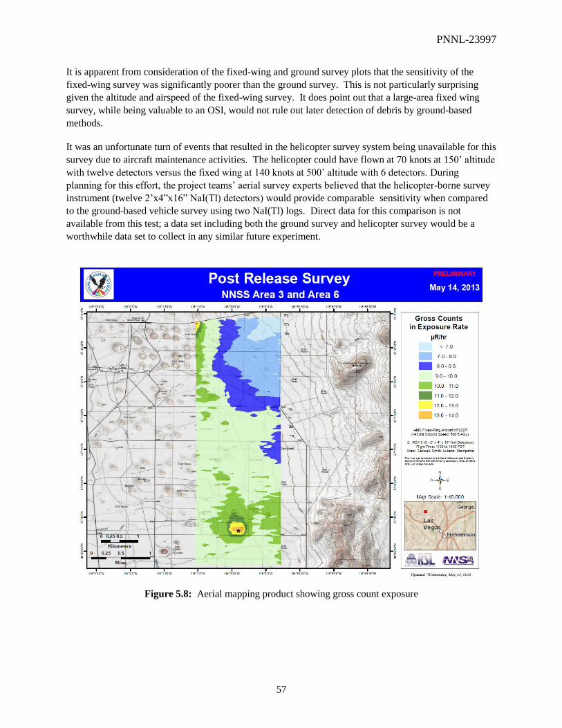
PNNL-23997
57
It is apparent from consideration of the fixed-wing and ground survey plots that the sensitivity of the
fixed-wing survey was significantly poorer than the ground survey. This is not particularly surprising
given the altitude and airspeed of the fixed-wing survey. It does point out that a large-area fixed wing
survey, while being valuable to an OSI, would not rule out later detection of debris by ground-based
methods.
It was an unfortunate turn of events that resulted in the helicopter survey system being unavailable for this
survey due to aircraft maintenance activities. The helicopter could have flown at 70 knots at 150’ altitude
with twelve detectors versus the fixed wing at 140 knots at 500’ altitude with 6 detectors. During
planning for this effort, the project teams’ aerial survey experts believed that the helicopter-borne survey
instrument (twelve 2’x4”x16” NaI(Tl) detectors) would provide comparable sensitivity when compared
to the ground-based vehicle survey using two NaI(Tl) logs. Direct data for this comparison is not
available from this test; a data set including both the ground survey and helicopter survey would be a
worthwhile data set to collect in any similar future experiment.
Figure 5.8: Aerial mapping product showing gross count exposure
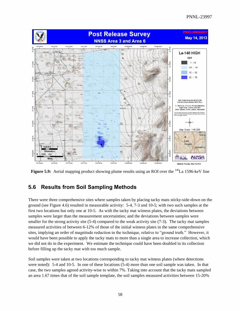
PNNL-23997
58
Figure 5.9: Aerial mapping product showing plume results using an ROI over the 140
La 1596-keV line
5.6 Results from Soil Sampling Methods
There were three comprehensive sites where samples taken by placing tacky mats sticky-side-down on the
ground (see Figure 4.6) resulted in measurable activity: 5-4, 7-3 and 10-5; with two such samples at the
first two locations but only one at 10-5. As with the tacky mat witness plates, the deviations between
samples were larger than the measurement uncertainties; and the deviations between samples were
smaller for the strong activity site (5-4) compared to the weak activity site (7-3). The tacky mat samples
measured activities of between 6-12% of those of the initial witness plates in the same comprehensive
sites, implying an order of magnitude reduction in the technique, relative to “ground truth.” However, it
would have been possible to apply the tacky mats to more than a single area to increase collection, which
we did not do in the experiment. We estimate the technique could have been doubled in its collection
before filling up the tacky mat with too much sample.
Soil samples were taken at two locations corresponding to tacky mat witness plates (where detections
were noted): 5-4 and 10-5. In one of these locations (5-4) more than one soil sample was taken. In that
case, the two samples agreed activity-wise to within 7%. Taking into account that the tacky mats sampled
an area 1.67 times that of the soil sample template, the soil samples measured activities between 15-20%

PNNL-23997
59
of those of the initial witness plates, or “ground truth”. However, it would have been possible to collect
larger soil samples than was done with the template, which we did not do in the experiment. We estimate
the technique could have been doubled in its collection before filling up the soil jars with too much
sample.
Vacuum samples were taken at a number of locations corresponding to tacky mat witness plates (where
detections were noted): 2-5, 5-4, and 6-3. Limited battery life prevented the taking of multiple samples
at one location. Taking into account that the tacky mats sampled an area 1.67 times that of the vacuumed
template, the vacuumed sample at 2-5 measured 10x the activity of the “ground truth” tacky mat witness
plate while at the other two locations the vacuumed samples measured 10-15% of the activity. We do not
have an explanation for the 2-5 results. We estimate the technique could have easily been increased a
factor of 4-5 times in its collection area before acquiring a full sample, assuming the power and cross
contamination issues are addressed.
Based on the above discussion, the soil and vacuum sampling techniques performed better in terms of
collecting more recently-deposited surface activity for a given area than applying tacky mats. When one
considers the amount of total recently deposited sample that can be collected, a vacuum approach is
clearly favored. Drawbacks of the vacuum approach, however, include cross-contamination of
equipment, and the ability to provide power to the equipment adequate to the time needed to take larger
samples. Further thought and design is needed in terms of how to include sample filters in the vacuum
cleaners. This technique would also be affected more so than soil samples if there were enough
precipitation so as to remove the radionuclides from the surface. Soil sampling, even though it obtains
much more soil depth than necessary for surface deposition, still provided reasonably robust samples in
this experiment.
MDAs based on Canberra Genie 2000 reporting for the limit-value soil and inverted tacky mat samples
indicated a typical range of ~1E-04 to 3E-04 Ci, although some samples were found to have MDAs
nearly an order of magnitude lower. Converting these to activity per unit area, based on the 18”x18”
sampling area, gives a range of ~4.8E-04 to 1.4E-03 Ci/m2. Finally, assuming the 10-20% comparison
for these sampling methods relative to the “ground truth” measurements of the large area witness plates
gives a typical MDA range of ~2.4E-03 to 1.4E-02 Ci/m2 detection sensitivity for samples brought to the
field laboratory. Several of the field laboratory measurements of these samples indicated significantly
lower MDAs.
5.7 In-Situ Measurements
Measurements with the LaBr3, NaI and HPGe handheld instuments were performed at a number of
locations. These locations are shown in Figure 5.10 and Table 5-5. The conversion of the count rate in the
1596 keV peak (140
La) to deposited activity is based upon MCNP simulation of the detection efficiency
for each detector, calculated as described previously for the vehicle survey. The simulated source was
based on a 40 meter radius disk.
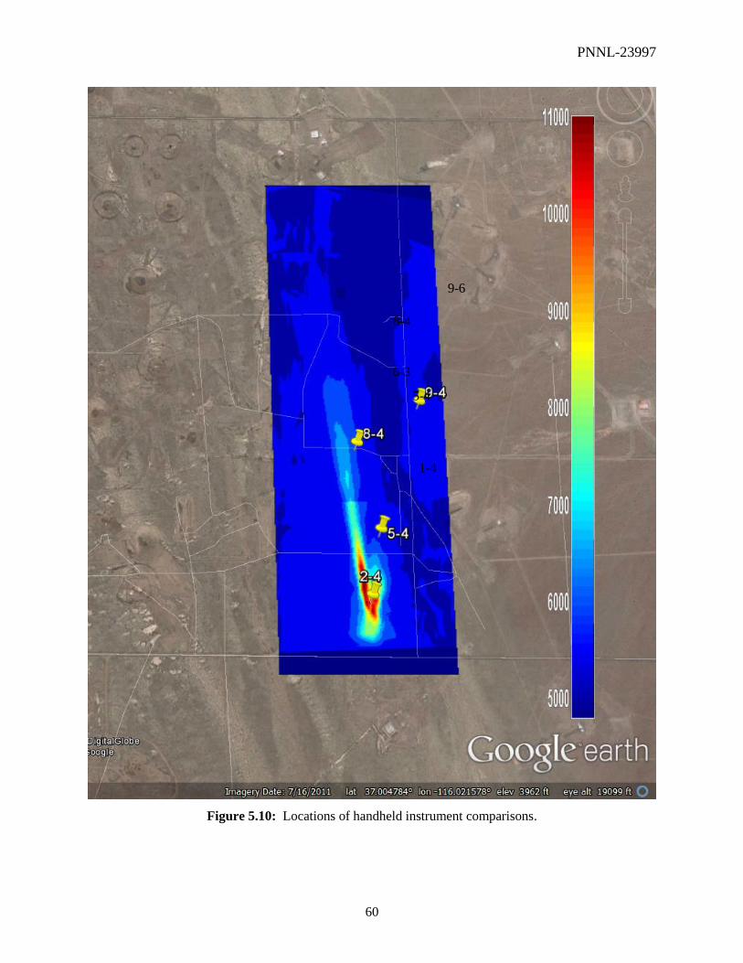
PNNL-23997
60
Figure 5.10: Locations of handheld instrument comparisons.
1-4
8-4
5-4
9-6
6-3
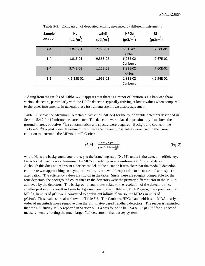
PNNL-23997
61
Table 5-5: Comparison of deposited activity measured by different instruments
Sample
Location
NaI
(µCi/m2
)
LaBr3
(µCi/m2
)
HPGe
(µCi/m2
)
RSI
(µCi/m2
)
2-4 7.04E-01 7.22E-01 5.01E-01
Ortec
7.50E-01
5-4 1.01E-01 9.35E-02 6.95E-02
Canberra
9.67E-02
8-4 9.74E-02 1.22E-01 8.83E-02
Ortec
7.60E-02
9-6 < 1.38E-02 1.96E-02 1.81E-02
Canberra
< 2.94E-02
Judging from the results of Table 5-5, it appears that there is a minor calibration issue between these
various detectors, particularly with the HPGe detectors typically arriving at lower values when compared
to the other instruments. In general, these instruments are in reasonable agreement.
Table 5-6 shows the Minimum Detectable Activities (MDAs) for the four portable detectors described in
Section 5.4.2 for 10 minute measurements. The detectors were placed approximately 1 m above the
ground in areas of active 140
La contamination and spectra were acquired. Background counts in the
1596 keV 140
La peak were determined from these spectra and those values were used in the Curie
equation to determine the MDAs in milliCuries:
𝑀𝐷𝐴 =4.65∗√𝑁𝐵+2.71
𝛾∗𝜀∗𝛵∗3.7𝑒4(𝐵𝑞
𝜇𝐶𝑖) (Eq. 2)
where NB is the background count rate, γ is the branching ratio (0.954), and ε is the detection efficiency.
Detection efficiency was determined by MCNP modeling over a uniform 40 m2 ground deposition.
Although this does not represent a perfect model, at the distance it was clear that the model’s detection
count rate was approaching an asymptotic value, as one would expect due to distance and atmospheric
attenuation. The efficiency values are shown in the table. Since these are roughly comparable for the
four detectors, the background count rates in the detectors were the primary differentiator in the MDAs
achieved by the detectors. The background count rates relate to the resolution of the detectors since
smaller peak-widths result in lower background count rates. Utilizing MCNP again, these point source
MDAs, in units of µCi, were converted to equivalent infinite plane source MDAs in units of
µCi/m2. These values are also shown in Table 5-6. The Canberra HPGe handheld has an MDA nearly an
order of magnitude more sensitive than the scintillator-based handheld detectors. The reader is reminded
that the RSI survey MDA reported in Section 5.1.1.4 was found to be 2.94 × 10⁻²
μCi/m2 for a 1 second
measurement, reflecting the much larger NaI detectors in that survey system.

PNNL-23997
62
Table 5-6: Table of MDAs for four detectors at 1 m height in terms of an infinite plane (modeled as a
uniform disk source 40 meters in diameter) for 10-minute acquisition times of 140
La’s 1596
keV Peak.
Detector ε (Efficiency) at 1596 keV MDA (Ci/m2)
at 1596 keV µCi/m2
FLIR NaI 3.98E-08 1.38E-02
Ludlum LaBr3 5.25E-08 1.24E-02
Ortec HPGe 3.51E-08 3.65E-03
Falcon HPGe 8.23E-08 2.00E-03
Comparing the sensitivities of the in-situ techniques reported in Table 5-6 to the soil sampling/field
laboratory measurements discussed in the previous section indicate that the most sensitive “typical” range
of soil measurements was comparable to the HPGe in-situ sensitivity, while the less sensitive “typical”
range was comparable to the scintillator in-situ sensitivity. The most sensitive MDA results for field
laboratory measurements were more sensitive than the in-situ systems. In general, it appears that the
sensitivities are roughly comparable, so that operational considerations would drive selection of the
techniques to emphasize for a given OSI scenario. For the PRex exercise, the authors believe that
significantly more samples could be collected and measured in the field laboratory, when compared to the
process of setting up and acquiring in-situ measurements in the field.
5.8 Comparison of Plume Modeling to Radiometric Results
Post-analysis of the release was performed using Hotshot 9 (Homann, 1994) using observed weather data,
and using a source injection height of 30 feet. The modeled and surveyed plume directions are in
agreement, although the lobe that extends in a more northerly direction is not indicated in the model. It
appears likely that this lobe was created by dispersal of material from the release point at a later time,
after the winds shifted more northerly.
Figure 5.11 shows deposition contours that are modeled when a source release of 1 Ci is assumed. These
contours indicate that the measurable plume would have extended significantly further downwind had the
full source been released. For example, the RSI survey instrument was previously reported to have an
MDA of ~ 3E-02 Ci/m2 for each 1 second interval. This indicates that the RSI survey would have been
capable of measuring the plume beyond the extent of the green contour in Figure 5.11. The following
figure (Figure 5.12), shows deposition contours based on a 0.07 Ci release, or the 7% release calculated
based on integration of the RSI ground survey data (paragraph 5.1.1.3). This Hotshot simulation of
deposition of the particulate La2O3 is much more consistent with the measured ground deposition,
although the measured plume does appear to be narrower than the modeled plume. This is likely due to
the short duration of the release: the model integrates over a 10 minute period.
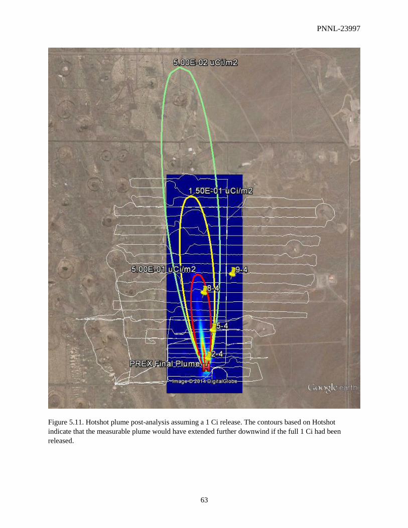
PNNL-23997
63
Figure 5.11. Hotshot plume post-analysis assuming a 1 Ci release. The contours based on Hotshot
indicate that the measurable plume would have extended further downwind if the full 1 Ci had been
released.
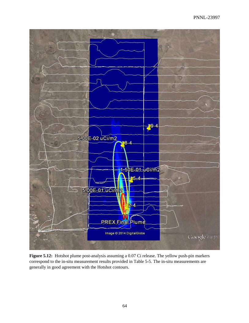
PNNL-23997
64
Figure 5.12: Hotshot plume post-analysis assuming a 0.07 Ci release. The yellow push-pin markers
correspond to the in-situ measurement results provided in Table 5-5. The in-situ measurements are
generally in good agreement with the Hotshot contours.

PNNL-23997
65
5.9 Optical Witness Plate Results
The objective to study short distance dispersion and fallout of lofted particulates benefits from detailed
knowledge of a number of important metrics. Knowledge of the size, shape and density of the particle to
be studied is perhaps the most fundamental starting point. Lofted elevation, followed by environmental
metrics including wind speed, turbulence, solar radiation, humidity, ambient particulate density and
character, and even ground terrain and foliage become important factors. This project strived to
characterize these parameters for Lanthanum Oxide powder that had been physically sieved and graded to
meet a size range around 40 µm. Once activated, the dispersion of this material could be detected with
radiation monitoring techniques. Some of these detection techniques, like the airborne detection systems,
would provide relatively low resolution indications of where the particles deposited on the ground.
Ground level radiation scans provide higher spatial resolution, and witness plates counted in the
laboratory provide specific spot information. Unfortunately, the spread of radioactive material to perform
these type of particulate dispersion surveys has inherent risks and certain unavoidable expense.
It was thought that if one could substitute non-radioactive particles that could be distinguished from
ubiquitous natural airborne particulate debris, that this substitute method could complement, or fully
replace the need to spread radioactive particulate for some future transport studies. Since the vast
majority of natural airborne soil is amorphous in shape, aluminosilicate glass microspheres were proposed
as a substitute particulate form. Aluminosilicate glass can be formulated with a range of densities,
allowing an approximate match to the average soil density of the Nevada desert. The aluminosilicate
microspheres can also be effectively graded to narrow size ranges by commercial manufactures. The
dispersion of multiple tightly controlled microsphere sizes would allow researchers to study, in a more
ideal way, the short range transport properties of fine particulate material.
Figure 5.13: Lanthanum oxide powder’s generally amorphous shape is visually indistinguishable from
ubiquitous desert airborne particulate.
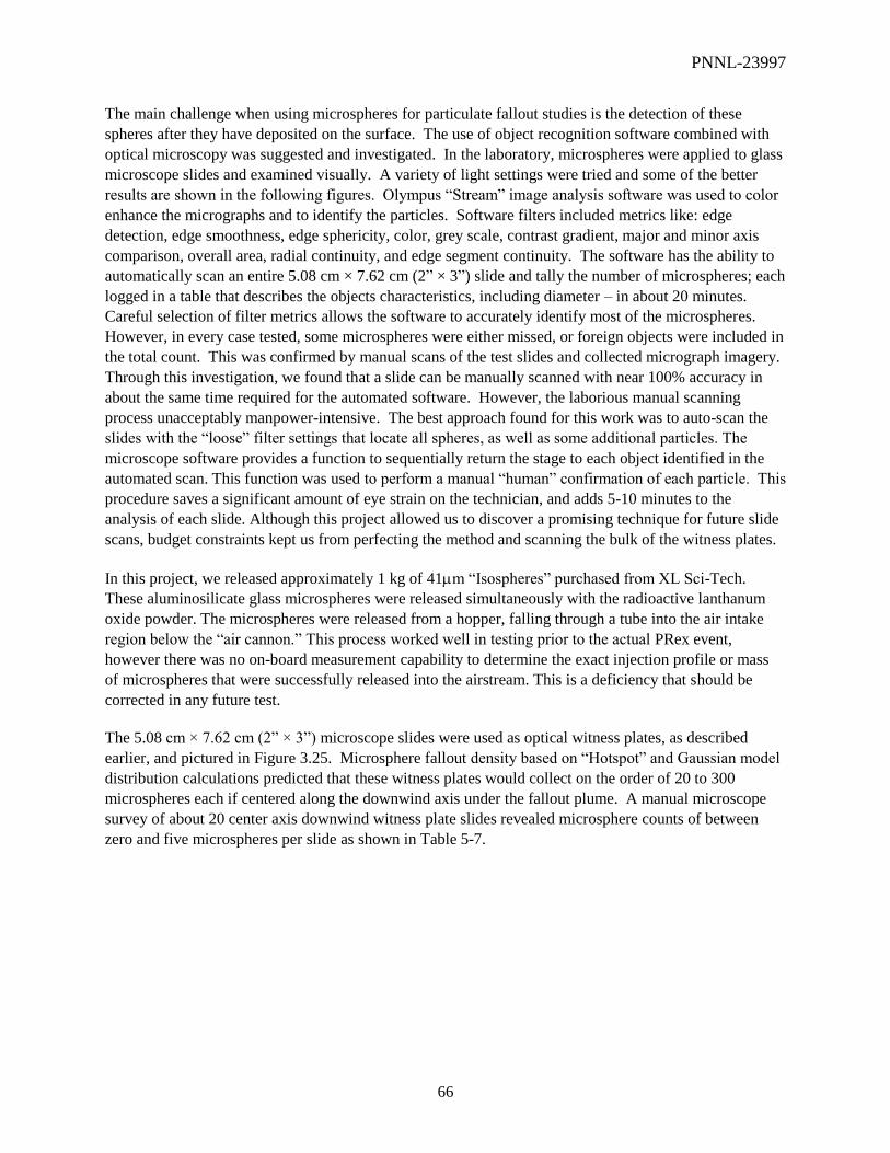
PNNL-23997
66
The main challenge when using microspheres for particulate fallout studies is the detection of these
spheres after they have deposited on the surface. The use of object recognition software combined with
optical microscopy was suggested and investigated. In the laboratory, microspheres were applied to glass
microscope slides and examined visually. A variety of light settings were tried and some of the better
results are shown in the following figures. Olympus “Stream” image analysis software was used to color
enhance the micrographs and to identify the particles. Software filters included metrics like: edge
detection, edge smoothness, edge sphericity, color, grey scale, contrast gradient, major and minor axis
comparison, overall area, radial continuity, and edge segment continuity. The software has the ability to
automatically scan an entire 5.08 cm × 7.62 cm (2” × 3”) slide and tally the number of microspheres; each
logged in a table that describes the objects characteristics, including diameter – in about 20 minutes.
Careful selection of filter metrics allows the software to accurately identify most of the microspheres.
However, in every case tested, some microspheres were either missed, or foreign objects were included in
the total count. This was confirmed by manual scans of the test slides and collected micrograph imagery.
Through this investigation, we found that a slide can be manually scanned with near 100% accuracy in
about the same time required for the automated software. However, the laborious manual scanning
process unacceptably manpower-intensive. The best approach found for this work was to auto-scan the
slides with the “loose” filter settings that locate all spheres, as well as some additional particles. The
microscope software provides a function to sequentially return the stage to each object identified in the
automated scan. This function was used to perform a manual “human” confirmation of each particle. This
procedure saves a significant amount of eye strain on the technician, and adds 5-10 minutes to the
analysis of each slide. Although this project allowed us to discover a promising technique for future slide
scans, budget constraints kept us from perfecting the method and scanning the bulk of the witness plates.
In this project, we released approximately 1 kg of 41m “Isospheres” purchased from XL Sci-Tech.
These aluminosilicate glass microspheres were released simultaneously with the radioactive lanthanum
oxide powder. The microspheres were released from a hopper, falling through a tube into the air intake
region below the “air cannon.” This process worked well in testing prior to the actual PRex event,
however there was no on-board measurement capability to determine the exact injection profile or mass
of microspheres that were successfully released into the airstream. This is a deficiency that should be
corrected in any future test.
The 5.08 cm × 7.62 cm (2” × 3”) microscope slides were used as optical witness plates, as described
earlier, and pictured in Figure 3.25. Microsphere fallout density based on “Hotspot” and Gaussian model
distribution calculations predicted that these witness plates would collect on the order of 20 to 300
microspheres each if centered along the downwind axis under the fallout plume. A manual microscope
survey of about 20 center axis downwind witness plate slides revealed microsphere counts of between
zero and five microspheres per slide as shown in Table 5-7.

PNNL-23997
67
Table 5-7. Beads collected by Optical Witness Plates at Various Sampling Locations. Figure 3.23 shows
the layout of the sampling locations; the first digit indicates the row, starting from row 0 at the south end
of the array. The second digit indicates the sampling location starting from position 1 at the west end of
each row. Appendix B also provides the coordinates for each location.
Slide Bead count
2-4 11
3-4 4
3-6 3
4-1 0
4-2 0
4-5 1
4-6 3
4-8-4 2
4-9 1
5-4-1 0
5-4-2 2
5-4-3 0
5-4-4 0
5-4-5 1
6-3 5
7-3-1 0
7-3-2 1
7-3-3 0
7-4 2
8-5 1
9-2-1 1
9-2-2 0
9-4 1

PNNL-23997
68
The low count statistics on these slides did not allow us to make a detailed correlation between the
radiation measurements and the optical counting results. However, it does appear that the bead detections
were consistent with the plume seen by radiation measurements. In particular, those sampling slides
showing the two highest numbers of beads, 2-4 and 6-3, correspond to the tacky mats showing the highest
measured radioactivity (see Appendix B) of the locations in the table above. It was found that
microspheres were successfully released, transported, collected, and subsequently measured via optical
microscopy. We saw no evidence that microspheres were “lost” once collected on the plates. The clear
adhesive surface presented to the microspheres seemed to hold them in place – even after significant
agitation while upside down and on edge. Visual inspection with the microscope along the edge frame of
the collection plates showed no “collection” of microspheres that may have released from their initial
deposition location. Likewise, no microspheres were found on the cover plates that were placed over the
witness plates before they were moved from their field location. This indicates that the method would
likely have been more successful (higher counting statistics) if a larger number of microspheres had been
released during the test.
The general technique using microspheres to provide well defined parametric study of short range particle
deposition showed promise, however additional instrumentation is needed to provide satisfactory results.
As with the radioactive particulates, a mechanism that provides a detailed record of the release (e.g. mass
per time) should be implemented. A greater number of witness plates would enhance the resolution of
results and hopefully guarantee that the deposition would be detected, no matter how narrow the plume.
Testing without the time restrictions associated with short half-life radioisotopes would allow staff to
release during the most favorable wind and weather conditions. Further investigation into the optimization
of microscope optics, lighting conditions, and image analysis software is also needed to efficiently count
microspheres on witness plates. Examples of methods developed during this work are provided in Figure
5.14 through Figure 5.18. The use of florescent or colored microspheres would also significantly enhance
the ability of image analysis software to identify the correct objects and count them with certainty.

PNNL-23997
69
Figure 5.14: A color-enhanced micrograph of aluminosilicate glass microspheres on a test slide similar
to the witness plates deployed during the NCNS test. Concentric rings around each sphere are the result
of dark field lighting; and create a unique visual signature for the microspheres compared to other debris
also shown.
Figure 5.15: Micrograph of aluminosilicate glass microspheres in dark field illumination without color
enhancement
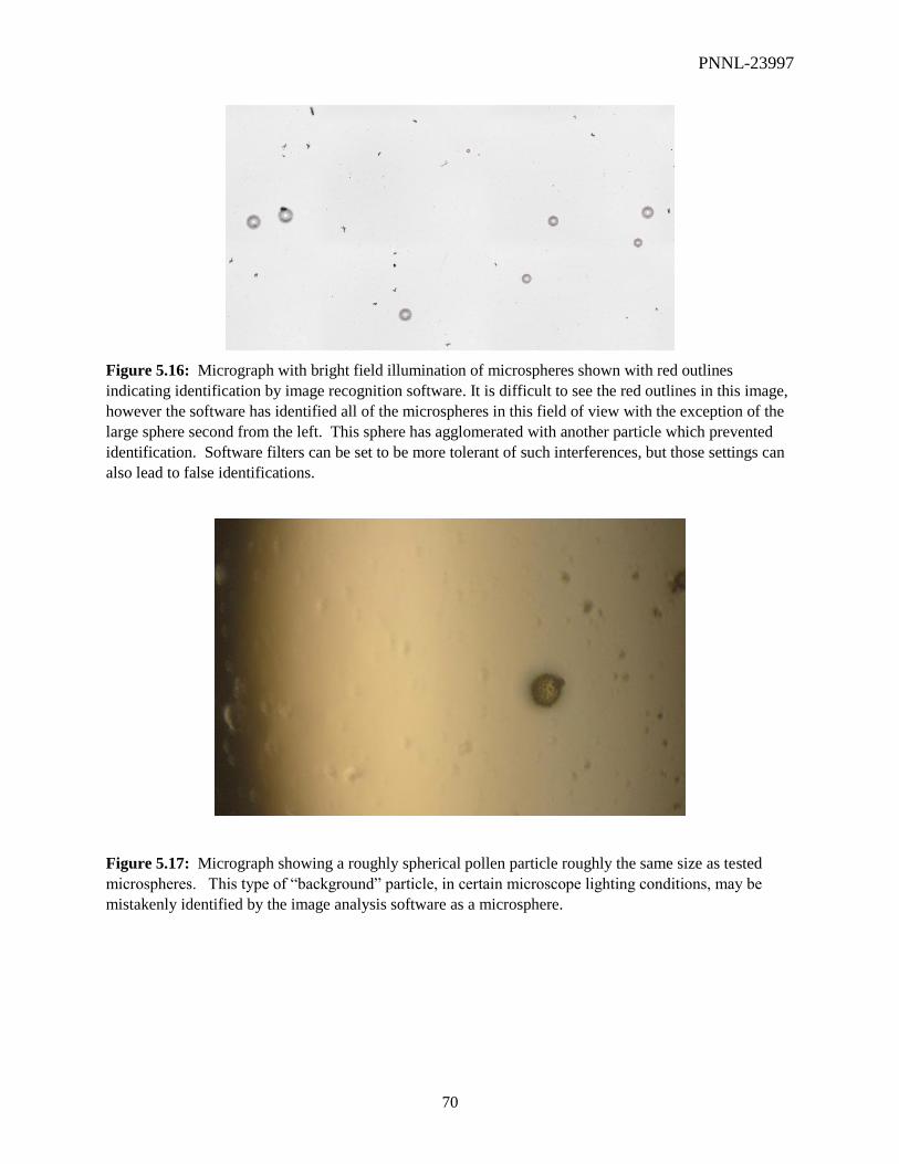
PNNL-23997
70
Figure 5.16: Micrograph with bright field illumination of microspheres shown with red outlines
indicating identification by image recognition software. It is difficult to see the red outlines in this image,
however the software has identified all of the microspheres in this field of view with the exception of the
large sphere second from the left. This sphere has agglomerated with another particle which prevented
identification. Software filters can be set to be more tolerant of such interferences, but those settings can
also lead to false identifications.
Figure 5.17: Micrograph showing a roughly spherical pollen particle roughly the same size as tested
microspheres. This type of “background” particle, in certain microscope lighting conditions, may be
mistakenly identified by the image analysis software as a microsphere.
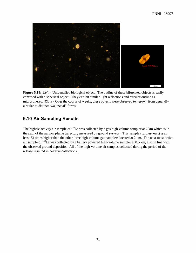
PNNL-23997
71
Figure 5.18: Left - Unidentified biological object. The outline of these bifurcated objects is easily
confused with a spherical object. They exhibit similar light reflections and circular outline as
microspheres. Right - Over the course of weeks, these objects were observed to “grow” from generally
circular to distinct two “pedal” forms.
5.10 Air Sampling Results
The highest activity air sample of 140
La was collected by a gas high volume sampler at 2 km which is in
the path of the narrow plume trajectory measured by ground surveys. This sample (furthest east) is at
least 33 times higher than the other three high-volume gas samplers located at 2 km. The next most active
air sample of 140
La was collected by a battery powered high-volume sampler at 0.5 km, also in line with
the observed ground deposition. All of the high-volume air samples collected during the period of the
release resulted in positive collections.

PNNL-23997
72
Figure 5.19: PAPR Air Sampler collections were consistent with the vehicle ground survey.
Background image provided by Google Earth.
The high volume gas samplers were restarted at 10 a.m. on the day following the release. None of the
samples collected on May 15th resulted in positive detection of
140La. The wind direction was generally
the same as on the day of release but the average speed was 3 m/s less than observed during the afternoon
of the release (10 m/s vs. 7 m/s). The maximum wind speed observed for each 15-minute interval is also
shown in Figure 5.21. There were ten maximum wind speed events greater than 14 m/s on May 14th, but
only one event approaching 12 m/s on the second day. The observed lower wind speeds, combined with
the large particle sizes, are most likely responsible for the lack of detectable lanthanum on the filters run
for resuspension on May 15.

PNNL-23997
73
Figure 5.20. Meteorological data from the weather station immediately south of the release point
The wind direction data in Figure 5.20 are not detailed enough to show the variation in wind direction
occurring immediately prior to the source release. Screen capture images of two-second interval
meteorological data was captured over the radio link from approximately 10 minutes before and after the
release (Figure 5.21). The gap in data is the result of reconfiguring the radio network to connect to and
activate the radio–controlled, battery-powered samplers located 1.5 km down range. Figure 5.21 shows
that the wind speed and direction varied during the time period leading up to the release, with lower wind
speeds associated with south-south-westerly winds, and higher wind speeds associated with south-south-
easterly winds (observed during release). The wind direction variation shown in Figure 5.21, particularly
right around the time of the source release, is consistent with the two-lobe plume deposition depicted in
Figure 5.3 and Figure 5.4.

PNNL-23997
74
Figure 5.21. Meteorological data captured from the weather station immediately south of the release
point.
A simple, low-cost Geiger-Mueller (GM) gamma detector was placed at the approach fence boundary
approximately 10 m up wind from the release point. The background count rate before the lid was
removed was approximately 1 cps. After the release, the gamma count was approximately 12 cps. A
second RM-80 gamma detector was placed adjacent to the filter of the battery-powered large volume
sampler at 1.5 km (grid 10-6). The recorded count rate at 1-minute intervals is shown in Figure 5.22. A
box car filter was run to generate the smoothed red line showing an increase in the count rate
approximately one minute after the sampler was activated. An outflow prop anemometer shows the
voltage increasing to 12 mV, equivalent to a flow of 1000 CFM (28.3 m3/min).
Figure 5.22. Count rate (blue) and smoothed count rate (red) of a GM tube monitoring sample collection
1.5 km downwind from the release. This sampler was remotely activated shortly before the release, and
the plume’s arrival can be observed during the sampling period.
PNNL-23997
75
6.0 Lessons Learned
6.1 Lessons Learned
During the course of the experiment, the team experienced and overcame a number of issues whose
impact could have been lessened with more detailed preparation. Preparing for the following items would
help to ensure a smoother experiment for any similar future effort. Some of these lessons would also be
valuable in planning for an On-Site Inspection. A number of these lessons are painfully obvious, however
are worth including in the list because they caused delays during the experiment execution. The same
types of issues are likely to plague both OSI exercises and any actual OSI in the future.
6.1.1 OSI-Relevant Lessons Learned
Survey navigation using GPS and the agricultural Raven light bar worked well. During our
background survey in September 2012, a significant amount of time and effort was spent in setting up a
grid of poles to allow relatively straight radiation survey lines to be driven with the off-road vehicle. In
the PRex test, the GPS + light bar navigation allowed the survey to be driven accurately on pre-
determined lines with no advance set-up.
Do not overestimate the ability to cover ground on foot. The going-in assumption for this experiment
was that much of the stake placement and pick-up would be on foot, but this was unrealistic. Even 2 km2
is a lot of territory and relatively short distances of 50 or 100 m can still be covered more quickly by
vehicle. This was particularly true in areas where smaller vegetation gave way to larger bushes and
Joshua trees. Had we chosen a site that could not be traversed by off-road vehicle, we would have had to
reduce our sampling area drastically.
Detectors should be calibrated for the expected source geometries before an experiment or
inspection. Much of the effort in preparing for the experiment was focused on preparation,
transportation, and release of the source. There were valid reasons for this, because a failure in these
areas would prevent execution of the experiment; however; this resulted in insufficient effort on prior
calibration of the various survey and measurement instruments for the geometries that would be
encountered. More advance preparation would have greatly simplified the subsequent analysis. The
work of calibrating instruments ahead of the expected survey and planning sample geometries should be a
main focus of OSI preparation. Wrangling through preparation of procedures, politics, etc., for an OSI
could take the place of the necessary focus on source preparation and delivery, leaving the inspection
team with the same calibration challenges that we faced.
All OSI operations need to be thought through with regard to situations where PPE is required.
For example, it was very difficult to drive while wearing the respirator. Originally, the filter part of the
respirator was on a person’s lower back, making sitting to drive impossible. Even moving the filter to a
person’s side still made sitting and driving very difficult. Detailed procedures documentation of
contamination levels requiring PPE should be in-place for an OSI. During this experiment, the RCTs
determined that respirators were not required after performing breathing-zone monitoring on the first
afternoon of work inside the contamination area.

PNNL-23997
76
Water policies while wearing PPE should be established. NNSS often allows Contamination Area
(CA) Radiological Work Permits (RWPs) to include a “one-water drink” option or internal camel-back
option, but this was not raised for us initially, so it was not addressed in the RWP. Staff would have been
able to stay in the field longer had these options been available. This will be a crucial issue for a warm-
weather OSI, when the PPE will rapidly cause inspectors to overheat, particularly if there is no provision
for water.
Vehicle-based ground survey provided the most comprehensive, useful data set. This suggests that
increased emphasis on highly sensitive vehicle survey instruments should be considered for OSI.
All OSI sampling operations need to be thought through in terms of windy conditions. We found it
very difficult to use plastic garbage bags for sample collection in winds beyond ~6 mph, though we did
succeed. Such wind speeds, or much faster, are very common in desert environments.
Collecting soil samples with tacky mats is difficult in windy conditions. Putting the tacky mat on the
ground and then folding it was very difficult in breezy conditions, and is definitely a two-person job.
Given the gravelly nature of the soil, these turned out to be a lot more bulky than we thought, and we
ended up putting them in collection jars rather than zip-lock bags.
Using a vacuum cleaner to collect samples presents a few challenges that need to be addressed. The
vacuum cleaner battery quickly lost power and, since it was in a CA, we could not take it back out for
recharging. It also presents a lot more cross-contamination risk than the other sampling techniques—
though some parts can be cleaned with wet wipes, the filters cannot without making them clog. Advance
practice is necessary in disassembling the vacuum cleaner over a sample jar, as not all material is
collected in the pre-filter panty hose.
Cross-contamination prevention procedures should be practiced in advance, in challenging (e.g.
dusty) conditions. We were not satisfied with the extent of the cross-contamination controls used in this
experiment. The back of the Mule was covered in kicked-up dust, and the witness tacky mats were not
sealed in their individual kitchen bags as we found it very difficult to use the small zip-ties with gloves
on. Results, however, seemed to indicate cross-contamination was not much of a problem. It may be that
in an on-site inspection, cross-contamination is not a paramount concern because the key objective is to
find relevant sampling locations rather than get a site perfectly mapped.
Dust masks and hats should be available for reducing exposure. It’s important to have a good supply
of dust masks to provide some protection when respirators are not required. Supplies included sufficient
respirators for use through the full sampling period. When RCTs determined that respirators were not
required, we found we did not have a sufficient supply of dust masks. It’s also useful to wear a hat or
other hair covering, even if a hood is not required, as a lot of dust can accumulate in exposed hair.
The use of each piece of OSI equipment should be thought through and practiced with regard to its
operational use in a Contamination Area. It can be very difficult to use detectors in a CA if they need
to be wrapped with plastic (to allow later removal from the CA for charging, other measurements, etc.).
The plastic wrapping can make using instrument controls difficult and viewing the screens impossible.
Radiation Control personnel may in some cases be willing to leave the screen exposed, and still clear the
instrument out of the CA.
PNNL-23997
77
Battery issues are an important consideration for field survey equipment. For example, the several
year-old batteries for the Canberra Falcon were weak and not able to run the detector for a useful length
of time. This required us to keep the Falcon plugged into the Mule’s battery. The tablet batteries also
died after a few hours, and then we could not use the Falcon system. We could also not bring the tablet
back out of the CA at this point due to contamination.
NaI(Tl) detectors, operated in singles mode in the field laboratory, were not found to be beneficial
to the experiment. Our initial thinking was that they would be useful screening tools for helping triage
which samples to measure first. However, at the activities involved, they did not offer any advantage
over the HPGe detectors. Operation of NaI(Tl) or other low-resolution detectors in coincidence mode
may offer more beneficial results.
In-situ HPGe survey and laboratory sample analysis provided roughly comparable sensitivities.
Field collection of samples followed by laboratory measurement appeared to be capable of more
throughput than in-situ measurements. In addition, field collection enabled longer counts (or overnight
counts) of interesting samples, and samples could be archived.
Laboratory sample analysis provided the highest sensitivity for ground deposition. It is, however,
hampered by the sparse data set relative to survey. This technique will be important in cases where OSI
ground survey does not find positive results, but interesting sites are identified by other techniques. It will
also be very useful to verify isotopes present if ground survey locates positive results.
Some data were lost due to the age of equipment and/or the age of remote radio communications
systems used during the test. It is best for the OSI team to use the most up-to-date equipment possible;
however, it is likely that an OSI team in the field will face similar equipment issues.
Verify local landmarks with a compass corrected for local deviation of magnetic north. Local staff
consistently referred to Tabletop Mt. for due north, however for our position on Yucca Flats this was not
entirely accurate. This resulted in misalignment of some portions of the release site, which needed to be
corrected after a compass was consulted.
Avoid the use of polarized sunglasses when working with electronic displays in the field. The
polarization of polarized sunglasses makes viewing electronic displays which make use of polarization in
the display mechanism difficult.
6.1.2 Experiment-Specific Lessons Learned
Tall stakes and flags are needed for visibility. The garden stakes were visible from 100 m away where
there was little brush, but very hard to see at distances beyond 100 m. The taller, wider wooden stakes
were easier to see, and held the flags in place better than the smooth metal garden stakes. Some flags slid
down to the ground on the garden stakes. Also, when attached to the tall wooden stakes, the flags were
less likely to snag on the sticky glass witness slides, which were sometimes placed near enough to the
garden stakes for flags to stick to them.

PNNL-23997
78
Calculate coordinates in advance. It would have been helpful to have had the proper stake coordinates
(in UTM form) in advance rather than having to calculate them on the spot. Occasionally, mistakes were
made that had to be corrected. This issue was corrected after a couple days during the set-up phase.
Duct tape and thin glass do not mix. The witness slides were originally to be taped to the holders with
packaging tape, but this was changed to duct tape due to concern about whether the tape would hold in the
wind. The duct tape adhesive was too strong, however, and some slides were broken in an attempt to
remove them. By the day after the release, the duct tape had adhered more strongly and entire garden
stakes had to be collected and then the tape cut off at the Conex processing table. Later, project staff had
to come up with a method to remove the tape so that it did not interfere with microscopy.
The experiment would have benefitted from an on-board method to quantify the total release and
its temporal profile. We had discussed a few methods of measuring the release of the radioactive
particles from the CO2 gerb but did not implement them due to time and funding-constraints. This created
challenges in the data analysis.
It is useful to determine where the plume is as soon as possible. Had we been able to determine this
earlier, it probably would have saved us time in the collection of the most relevant samples; most of the
first day we only knew the general area of the plume, assuming that the release had truly been successful.
The large area witness plates need more rigid frames. The tacky mats were warped by their staking
and exposure for a few days. They no longer closed like a book but stuck out at the corners and didn’t
really stick together at all. Putting the plates with backing into the bags was then quite difficult; they
often caught on the bags, even without the strong wind causing havoc.
PNNL-23997
79
7.0 Conclusions and Recommendations
The PRex radionuclide release test was successfully conducted during the week of May 13th, 2013. The
experiment, designed to mimic a small vent of radioparticulates from an underground nuclear explosion,
involved lofting approximately 1 Ci of 140
La in the form of 32-45 micron-sized La2O3 powder via an air
cannon. Integration of the deposited plume data collected with vehicle ground survey indicates that ~7%
of the activity in the original source was deposited within the plume area. Despite this deposition value
being lower than planned, the plume provided an opportunity to collect detailed vehicle-based ground
survey, and provided positive results on soil, air sample, and aerial survey. The data collected allowed for
comparison of the sensitivity of survey and sampling methods. Many Lessons Learned for both planning
a similar future experiment and conducting a future OSI were collected.
The vehicle ground survey was found to provide the most comprehensive data set for characterizing the
location and deposition activity in the plume. This method also allowed the ground-based experiment
team to cover the most area relative to the time invested. However, the ground-based vehicle survey was
not as sensitive as the in-situ and sampling techniques employed. The narrowness of the plume, only a
couple 100m, showed that survey and sampling techniques must cover a comparably tight spacing or risk
missing a plume for a radioactive vent.
In-situ measurements with HPGe detectors were found to be roughly an order of magnitude more
sensitive than comparable measurements with scintillator-based detectors, which were themselves more
sensitive than the vehicle ground survey. The sensitivity of soil samples measured in the field laboratory
was roughly comparable to the in-situ HPGe measurements, although some laboratory sample
measurements achieved more sensitive results. From this work, it appears that the selection of emphasis
between in-situ vs. sampling/field laboratory measurements should be based on throughput capability and
other operational considerations (e.g. ability to archive samples). Both methods provide useful capability
to an inspection team. However, the data provided is sparse compared to vehicle-based ground survey and
should be focused on areas identified as interesting through other techniques.
The backpack survey results did not provide significant sensitivity enhancement over vehicle survey in
the Kawasaki mule. Further, this survey method is very slow compared to vehicle-based survey.
Backpack survey should only be used in situations where vehicle survey is not possible, or when the
backpack is carried by an inspection team member who is performing other duties.
The fixed-wing aerial survey performed for this work was flown at 500 feet AGL, with 500-ft line
spacing, at 140 knots. These flight parameters limited the sensitivity of the aerial survey; however, they
are realistic for a large area, fixed-wing survey during an OSI. The survey provided a positive detection
of the source dispersal location, and a weak indication of the presence and direction of the deposited
plume. A helicopter-based survey, flown at lower elevation and closer line spacing, would have provided
a much more detailed map of the plume.
Three soil sampling techniques were used during this experiment: troweling the top layer of soil,
collecting the lightest dust and debris using a handheld vacuum cleaner, and collecting the top-most soil
and pebbles using an inverted tacky mat. All of these methods were observed to provide surface activity
level estimates that were low compared to the “ground truth” values determined through measurement of
the large-area witness plate samples, roughly in the range of 6% to 20%. A rough ordering of the

PNNL-23997
80
techniques in terms of percent of “ground truth” activity collected, for the same surface areas, was 1)
trowel soil collection, 2) vacuum cleaner, and 3) inverted tacky mat; however, the latter two techniques
could easily be designed to collect from larger areas than were used in our soil collection. The vacuum
cleaner method appeared to provide a good technique for collecting recent debris, but suffered from poor
battery life and high potential for cross-contamination. The tacky-mat method also collected a sample
from mainly the top layer of soil, but is challenging to accomplish during windy conditions. Calibration
of the measurement geometry for the bulky tacky mats with soil is also challenging. Troweling a surface
layer of soil was relatively straight forward, allows for good contamination control, and provides a
repeatable sample geometry for laboratory measurement. This is also likely the best approach for
inspections that occur later in terms of time after a detonation event, when radionuclide debris may have
migrated downward into the soil.
The use of inert microspheres and optical microscopy methods did not provide sufficient results to define
the deposition plume, though they did appear to track with the radiation plume. Microspheres were
successfully collected and identified on optical witness plates downwind from the release. In order to use
this method to produce viable results, it would be necessary to release a larger quantity of microspheres.
The use of colored or fluorescent microspheres would also aid in discriminating the released microspheres
from naturally occurring spherical particles.
7.1 Recommended Future Work
A significant portion of the effort in the PRex experiment revolved around the successful preparation,
transport, and release of the radionuclide source. Based on this experience, this portion of the work
would be more straightforward for a future effort, and would allow more emphasis on areas that were not
fully developed in this test. For example, more detailed information on the release timing (e.g., activity
injected into the atmosphere vs. time) and injection levels into the atmosphere would provide for
improved atmospheric modeling of the release. This would also provide better knowledge of the release
quantity. Utilizing a longer release time (~10 minutes) could also be beneficial in comparisons to
meteorological modeling.
Delays in the manufacturing of the radioactive microspheres originally expected to be used in this work
forced the use of sieved La2O3 powder. The microspheres would have provided a much more uniform
and well known particle size distribution for use in modeling the deposition. Future work utilizing
radioactive microspheres would provide a more detailed dataset for comparison to meteorological
modelling results. The use of microspheres in different size ranges, tagged with different radioisotopes,
would also allow investigation of the atmospheric transport of multiple particle sizes in a single
experiment.
Besides use of microspheres and more controlled releases, as discussed in the previous two paragraphs,
another area for potential follow-on work concerns the transport of particulates within subsurface
fractures, which is poorly understood. This could involve experiments from shallow tunnels or a large
lysimeter. Having successfully produced a vent scenario in PRex, one could also envision involving more
participants in a future exercise, in line with a recent release exercise in Canada. United Kingdom
colleagues from the Atomic Weapons Establishment have expressed an interest in participating in such an
exercise.
PNNL-23997
81
8.0 References
Forster, RA, LJ Cox, RF Barrett, TE Booth, JF Briesmeister, FB Brown, JS Bull, GC Geisler, JT Goorley,
RD Mosteller, SE Post, RE Prael, EC Selcow, and A Sood. 2004. "Mcnp™ Version 5." Nuclear
Instruments and Methods in Physics Research Section B: Beam Interactions with Materials and Atoms
213:82-86. 10.1016/s0168-583x(03)01538-6.
Homann, SG. 1994. "Hotspot Heath Physics Codes for the Pc." Lawrence Livermore National
Laboratory.
Lyons, C. 2012. Aerial Measuring System (Ams) Baseline Surveys for Emergency Planning. Presented at
22nd Annual RETS-REMP Workshop, Orlando, FL, Nuclear Energy Institute, Washington, D.C.
Seifert, AH, LM Arrigo, JEB Jr., RS Detwiler, ME Keillor, WJ Kernan, RR Kirkham, BD Milbrath, JP
Rishel, CE Seifert, and JE Smart. 2013. Particle Release Experiment (Prex) Plan. Report No. PNNL-SA-
95357, Pacific Northwest National Laboratory, Richland, WA.
Smart, JE. 2013. Aluminum Can Liner Design Considerations. Report No. PNNL-SA-95023, Pacific
Northwest National Laboratory, Richland, WA.

PNNL-23997
A.1
Appendix A
Ground Vehicle Survey Data Corrections
This appendix provides details of the data analysis methods applied to correct errors and lost data in the
original data set.
A.1 Introduction
The RSI ground survey data collected on Wednesday, May 15th and Thursday, May 16
th suffered from
two distinct data corruption problems. The first occurred because the RSI automatic energy calibration
function occasionally recalibrated on the 1596 keV peak of 140
La rather than on the correct 1461 keV peak
of 40
K. This occurred despite the fact that the auto calibration mode was inhibited during the collection;
activation of the auto calibration appears to be correlated to the second problem, data drop-outs, discussed
next. The survey system generally corrected the energy calibration as the count rate from 140
La dropped,
and the background 40
K peak came to the fore. However, for the final hour of the third survey period, one
of the two detectors remained incorrectly calibrated.
The second data corruption issue was a loss of data collection that tended to occur after the system
transited the peak count rate encountered during transepts of the plume. These outages consistently
occurred after the peak rate had been observed, during the downward trend in count rate. They did not
consistently affect both of the survey detectors; there are times when data from one detector was not
collected, and there are fewer times when data from both detectors were not collected. This appendix
provides a description of the methods used to 1) correct the energy calibration in cases where the system
incorrectly identified the 1596 keV 140
La peak as the 1461 keV 40
K peak, and 2) fill in the missing data to
allow contouring and integration of the deposited plume.
A.2 Data Correction
The following method was adopted to sum the spectra from the two NaI(Tl) detectors at each 1-second
time interval. The method was applied to each of the individual surveys, i.e., May15 AM, May15 PM and
May16. The steps were followed in order for all corrected survey data to ensure the desired data
correction was obtained.
1. Recalibrate NaI(Tl) detector data to 40
K – last hour and at several peaks
2. Where only one log is present – scale counts to other log’s average and add to existing data
3. Where two logs are missing – interpolate from both directions in time. The interpolation was applied
on a channel by channel basis for the spectra.
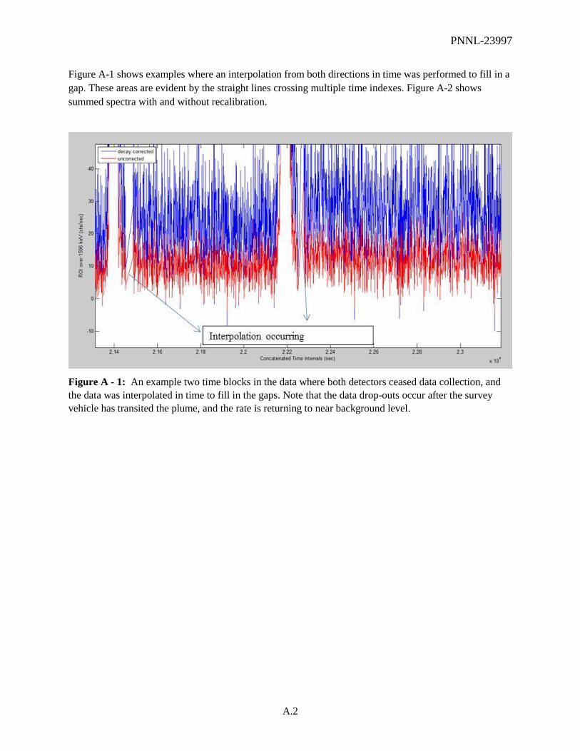
PNNL-23997
A.2
Figure A-1 shows examples where an interpolation from both directions in time was performed to fill in a
gap. These areas are evident by the straight lines crossing multiple time indexes. Figure A-2 shows
summed spectra with and without recalibration.
Figure A - 1: An example two time blocks in the data where both detectors ceased data collection, and
the data was interpolated in time to fill in the gaps. Note that the data drop-outs occur after the survey
vehicle has transited the plume, and the rate is returning to near background level.

PNNL-23997
A.3
Figure A - 2: NaI(Tl) spectral data, before and after correction of the energy calibration. Note that the
corrected data has the false peaks below the 40
K and 208
Tl peaks removed.
The next two figures show the results of the data repair for the May 15th AM survey and the May 16
th
surveys. Although the figures just show gross counts, the repairs were performed on the component
energy channels. The repairs to the Wednesday morning data (“May 15 AM”) occurred only during one
timeframe, after transit of the plume. Data from the Wednesday afternoon survey (“May 15 PM”) did not
require correction. This data set was collected further downwind, and did not include high 140
La count
rate data. The survey on May 16th required extensive correction due to both energy calibration and data
drop-out issues. The last ~4000 seconds required extensive energy recalibration of data from one of the
NaI(Tl) detectors.

PNNL-23997
A.4
Figure A - 3: Data correction required due to data drop-out from one of the two NaI(Tl) detectors on
Wednesday morning. The drop-out occurred after the survey crossed the plume on the closest-in transept
of Wednesday (thus the highest count rate for the day). This correction was of the 2nd
variety (one
detector drop-out).

PNNL-23997
A.5
Figure A - 4: More extensive corrections were required for the Thursday morning survey data, which
suffered more frequent data corruption issues. The red trace (raw data) is directly behind the blue
(corrected data) where it does not show. Time periods where the red trace drops to zero indicate that both
detectors stopped data collection after transiting the plume (corrected with interpolation). Drops to ~3000
cps indicate a single detector dropped out (corrected based on the operating detector rate).
After correction, the three surveys were concatenated into one file for further data processing, plume
plotting, and plume activity integration. The corrected data were used to develop estimates of the total
activity deposited within the plume, as discussed in the main report.

PNNL-23997
B.1
Appendix B
Field Laboratory Gamma Assay Results
The following table contains analysis results for the HPGe-based field laboratory sample measurements of PRex samples. PNNLWD57752 and
PNNL WD66091 are two ~50% relative efficiency Canberra P-type crystals (Figure 4.14). The NSTec column provides results from the portable
Canberra extended-range P-type detector provided and operated by NSTec (Figure 4.16).
Table A - 1: Gamma Assay Results
Sample
Location easting northing Sample Type
PNNL WD57752
(uCi)
PNNL WD66091
(uCi) NSTec (uCi)
MDA
(uCi) Notes
0-1 588277 4094865 Tacky Mat
No Detect
2.01 E-5 No Detect
0-2 588377 4094865 Tacky Mat No Detect
1.51 E-5 No Detect
0-3 588477 4094865 Tacky Mat
Not Counted
1-1 588177 4094965
Not Counted
1-2 588277 4094965 Tacky Mat No Detect
3.79 E-5 No Detect
2-1 588077 4095065
Not Counted
2-2 588177 4095065 Tacky Mat No Detect
2.39 E-5 No Detect
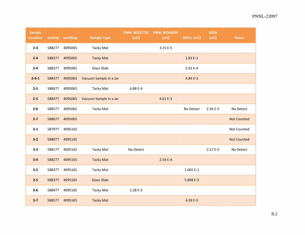
PNNL-23997
B.2
Sample
Location easting northing Sample Type
PNNL WD57752
(uCi)
PNNL WD66091
(uCi) NSTec (uCi)
MDA
(uCi) Notes
2-3 588277 4095065 Tacky Mat
3.15 E-5
2-4 588377 4095065 Tacky Mat
1.83 E-1
2-4 588377 4095065 Glass Slide
5.91 E-4
2-4-1 588377 4095065 Vacuum Sample in a Jar
4.84 E-3
2-5 588477 4095065 Tacky Mat 6.88 E-4
2-5 588477 4095065 Vacuum Sample in a Jar
4.61 E-3
2-6 588577 4095065 Tacky Mat
No Detect 2.56 E-5 No Detect
2-7 588677 4095065
Not Counted
3-1 587977 4095165
Not Counted
3-2 588077 4095165
Not Counted
3-3 588177 4095165 Tacky Mat No Detect
2.17 E-5 No Detect
3-4 588277 4095165 Tacky Mat
2.54 E-4
3-5 588377 4095165 Tacky Mat
1.065 E-1
3-5 588377 4095165 Glass Slide
5.898 E-5
3-6 588477 4095165 Tacky Mat 2.28 E-3
3-7 588577 4095165 Tacky Mat
4.59 E-5

PNNL-23997
B.3
Sample
Location easting northing Sample Type
PNNL WD57752
(uCi)
PNNL WD66091
(uCi) NSTec (uCi)
MDA
(uCi) Notes
3-8 588677 4095165 Tacky Mat No Detect
1.53 E-5 No Detect
3-9 588777 4095165 Tacky Mat
No Detect 1.77 E-5 No Detect
3-10 588877 4095165
Not Counted
4-1 587977 4095265
Not Counted
4-2 588077 4095265 Tacky Mat
No Detect
2.21 E-5 No Detect
4-2 588077 4095265 PAPR Air Filter
2.42 E-4
4-3 588177 4095265 Tacky Mat
No Detect 1.74 E-5 No Detect
4-3 588177 4095265 PAPR Air Filter
2.40 E-5
4-4 588277 4095265 Tacky Mat 2.81 E-4
4-4 588277 4095265 Glass Slide No Detect
4.35 E-5 No Detect
4-4-4 ft 588277 4095265 PAPR Air Filter
1.21 E-4
4-4-22 ft 588277 4095265 PAPR Air Filter
No Detect
3.90 E-5 No Detect
4-4-45 ft 588277 4095265 PAPR Air Filter
1.44 E-4
4-5 588377 4095265 Glass Slide 1.589 E-4
4-5.5 588427 4095265 PAPR Air Filter 1.78 E-2
half way
between 4-5 &
4-6

PNNL-23997
B.4
Sample
Location easting northing Sample Type
PNNL WD57752
(uCi)
PNNL WD66091
(uCi) NSTec (uCi)
MDA
(uCi) Notes
4-6 588477 4095265 Tacky Mat 2.04 E-2
4-6 588477 4095265 PAPR Air Filter
3.54 E-3
4-6-4 ft 588477 4095265 PAPR Air Filter
6.28 E-3
4-6-22 ft 588477 4095265 PAPR Air Filter
3.96 E-4
4-6-45 ft 588477 4095265 PAPR Air Filter
4.72 E-3
4-7 588577 4095265 Tacky Mat
1.09 E-4
4-7 588577 4095265 PAPR Air Filter
3.61 E-5
4-8 588677 4095265 PAPR Air Filter
No Detect 4.50 E-5 No Detect
4-8-1 588677 4095265 Tacky Mat
2.43 E-5
4-8-2 588677 4095265 Tacky Mat
1.48 E-4
4-8-3 588677 4095265 Tacky Mat 3.06 E-5
4-8-4 588677 4095265 Tacky Mat
6.45 E-5
4-8-5 588677 4095265 Tacky Mat 4.69 E-5
4-9 588777 4095265 Tacky Mat No Detect
6.52 E-6 No Detect
4-10 588877 4095265 Tacky Mat No Detect
1.79 E-5 No Detect
4-11 588977 4095265
Not Counted

PNNL-23997
B.5
Sample
Location easting northing Sample Type
PNNL WD57752
(uCi)
PNNL WD66091
(uCi) NSTec (uCi)
MDA
(uCi) Notes
4-12 589077 4095265
Not Counted
5-1 587877 4095365
Not Counted
5-2 588027 4095365
Not Counted
5-3 588227 4095365 Tacky Mat 1.26 E-4
5-4-1 588427 4095365 Tacky Mat 3.98 E-2
5-4-1 588427 4095365 Tacky Mat Jar
2.8 E-3 3.175 E-3
5-4-1 588427 4095365 Soil Jar 9.05 E-3 8.55 E-3 1.00 E-2
5-4-2 588427 4095365 Tacky Mat
3.22 E-2
5-4-2 588427 4095365 Tacky Mat Jar
2.616 E-3
5-4-2 588427 4095365 Glass Slide
3.27 E-5
5-4-2 588427 4095365 Soil Jar
8.56 E-3
5-4-3 588427 4095365 Tacky Mat 3.42 E-2
5-4-4 588427 4095365 Tacky Mat
4.30 E-2
5-4-4 588427 4095365 Vacuum Sample in a Jar
3.39 E-3
5-4-5 588427 4095365 Tacky Mat 3.89 E-2
5-5 588627 4095365 Tacky Mat 7.68 E-5

PNNL-23997
B.6
Sample
Location easting northing Sample Type
PNNL WD57752
(uCi)
PNNL WD66091
(uCi) NSTec (uCi)
MDA
(uCi) Notes
5-6 588827 4095365
Not Counted
5-7 589052 4095365
Not Counted
5-8 589227 4095365
Not Counted
6-1 587927 4095465
Not Counted
6-2 588177 4095465 Tacky Mat
No Detect
9.55 E-6 No Detect
6-2 588177 4095465 PAPR Air Filter
No Detect
1.13 E-5
6-2 588177 4095465 Glass Slide
No Detect 2.13 E-5 No Detect
6-3 588327 4095465 Tacky Mat
5.19 E-1
6-3 588327 4095465 Vacuum Sample in a Jar 1.16 E-2
6-4 588527 4095465 PAPR Air Filter
1.48 E-4 1.499 E-4
6-4 588527 4095465 Tacky Mat
Not Counted
6-5 588727 4095451 PAPR Air Filter
No Detect 3.72 E-5
6-5 588727 4095451 Tacky Mat
Not Counted
6-6 588902 4095465 Tacky Mat
Not Counted
6-7 589127 4095465 Tacky Mat
Not Counted
6-8 589327 4095465 Tacky Mat
Not Counted

PNNL-23997
B.7
Sample
Location easting northing Sample Type
PNNL WD57752
(uCi)
PNNL WD66091
(uCi) NSTec (uCi)
MDA
(uCi) Notes
7-1 587827 4095565
Not Counted
7-2 588027 4095565 Tacky Mat
No Detect
5.04 E-5 No Detect
7-3-1 588227 4095565 Tacky Mat 6.45 E-4
7-3-1 588227 4095565 Soil Jar
No Detect 6.13 E-5
7-3-2 588227 4095565 Tacky Mat
1.79 E-4
7-3-2 588227 4095565 OSI Tacky Mat 2.95 E-5
7-3-3 588227 4095565 Tacky Mat
9.33 E-4
7-3-4 588227 4095565 Tacky Mat
1.12 E-3
7-3-4 588227 4095565 OSI Tacky Mat 6.8 E-5
7-3-5 588227 4095565 Tacky Mat 4.71 E-4
7-4 588427 4095565 Tacky Mat 2.23 E-2
7-5 588627 4095565 Tacky Mat
No Detect
9.35 E-5 No Detect
7-6 588827 4095581
Not Counted
7-7 589027 4095565
Not Counted
7-8 589227 4095565
Not Counted
7-9 589427 4095565
Not Counted

PNNL-23997
B.8
Sample
Location easting northing Sample Type
PNNL WD57752
(uCi)
PNNL WD66091
(uCi) NSTec (uCi)
MDA
(uCi) Notes
8-1 587727 4095765
Not Counted
8-2 587927 4095765
Not Counted
8-3 588127 4095765 Tacky Mat
No Detect 5.73 E-5 No Detect
8-4 588327 4095765 Tacky Mat 2.64 E-2
8-5 588527 4095765 Tacky Mat
1.15 E-3
8-5 588527 4095765 Glass Slide
No Detect No Detect 1.31 E-4
8-6 588727 4095765 Tacky Mat
1.76 E-4
8-7 588927 4095765 Tacky Mat
3.122 E-5
8-8 589127 4095765 Tacky Mat
No Detect 1.63 E-5 No Detect
8-9 589327 4095765 Tacky Mat
No Detect
8.95 E-6 No Detect
8-10 589427 4095765
Not Counted
9-1 587627 4095965
Not Counted
9-2-1 587827 4095965 Tacky Mat
No Detect
1.99 E-5 No Detect
9-2-2 587827 4095965 Tacky Mat No Detect
5.16 E-5 No Detect
9-2-2
Glass Slide No Detect
6.56 E-6 No Detect
9-2-3 587827 4095965 Tacky Mat
7.82 E-4
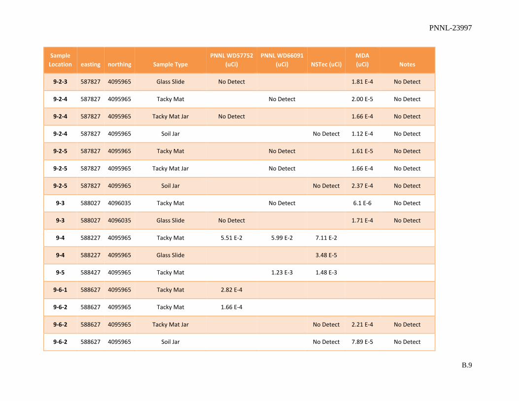
PNNL-23997
B.9
Sample
Location easting northing Sample Type
PNNL WD57752
(uCi)
PNNL WD66091
(uCi) NSTec (uCi)
MDA
(uCi) Notes
9-2-3 587827 4095965 Glass Slide No Detect
1.81 E-4 No Detect
9-2-4 587827 4095965 Tacky Mat
No Detect
2.00 E-5 No Detect
9-2-4 587827 4095965 Tacky Mat Jar No Detect
1.66 E-4 No Detect
9-2-4 587827 4095965 Soil Jar
No Detect 1.12 E-4 No Detect
9-2-5 587827 4095965 Tacky Mat
No Detect
1.61 E-5 No Detect
9-2-5 587827 4095965 Tacky Mat Jar
No Detect
1.66 E-4 No Detect
9-2-5 587827 4095965 Soil Jar
No Detect 2.37 E-4 No Detect
9-3 588027 4096035 Tacky Mat
No Detect
6.1 E-6 No Detect
9-3 588027 4096035 Glass Slide No Detect
1.71 E-4 No Detect
9-4 588227 4095965 Tacky Mat 5.51 E-2 5.99 E-2 7.11 E-2
9-4 588227 4095965 Glass Slide
3.48 E-5
9-5 588427 4095965 Tacky Mat
1.23 E-3 1.48 E-3
9-6-1 588627 4095965 Tacky Mat 2.82 E-4
9-6-2 588627 4095965 Tacky Mat 1.66 E-4
9-6-2 588627 4095965 Tacky Mat Jar
No Detect 2.21 E-4 No Detect
9-6-2 588627 4095965 Soil Jar
No Detect 7.89 E-5 No Detect
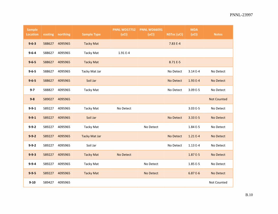
PNNL-23997
B.10
Sample
Location easting northing Sample Type
PNNL WD57752
(uCi)
PNNL WD66091
(uCi) NSTec (uCi)
MDA
(uCi) Notes
9-6-3 588627 4095965 Tacky Mat
7.83 E-4
9-6-4 588627 4095965 Tacky Mat 1.91 E-4
9-6-5 588627 4095965 Tacky Mat
8.71 E-5
9-6-5 588627 4095965 Tacky Mat Jar
No Detect 3.14 E-4 No Detect
9-6-5 588627 4095965 Soil Jar
No Detect 1.93 E-4 No Detect
9-7 588827 4095965 Tacky Mat
No Detect 3.09 E-5 No Detect
9-8 589027 4095965
Not Counted
9-9-1 589227 4095965 Tacky Mat No Detect
3.03 E-5 No Detect
9-9-1 589227 4095965 Soil Jar
No Detect 3.33 E-5 No Detect
9-9-2 589227 4095965 Tacky Mat
No Detect
1.84 E-5 No Detect
9-9-2 589227 4095965 Tacky Mat Jar
No Detect 1.21 E-4 No Detect
9-9-2 589227 4095965 Soil Jar
No Detect 1.13 E-4 No Detect
9-9-3 589227 4095965 Tacky Mat No Detect
1.87 E-5 No Detect
9-9-4 589227 4095965 Tacky Mat
No Detect
1.85 E-5 No Detect
9-9-5 589227 4095965 Tacky Mat
No Detect
6.87 E-6 No Detect
9-10 589427 4095965
Not Counted
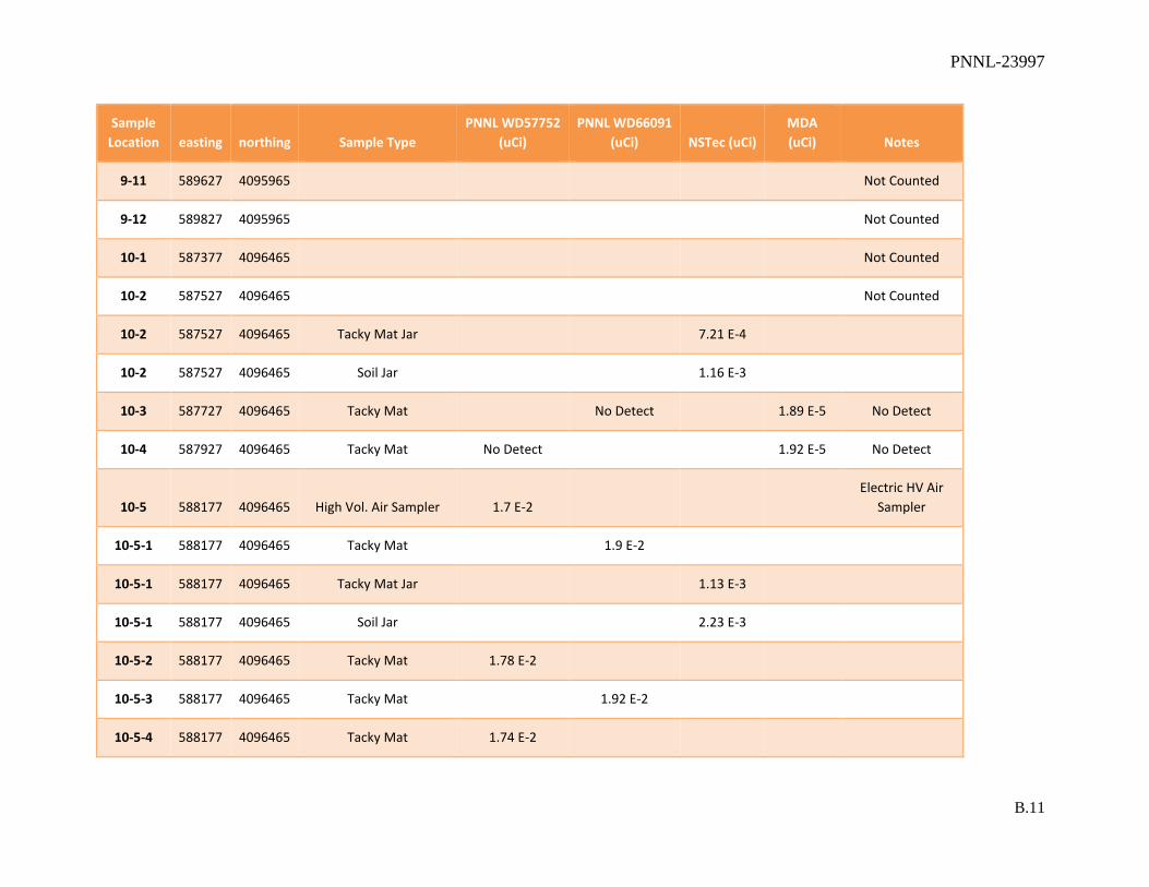
PNNL-23997
B.11
Sample
Location easting northing Sample Type
PNNL WD57752
(uCi)
PNNL WD66091
(uCi) NSTec (uCi)
MDA
(uCi) Notes
9-11 589627 4095965
Not Counted
9-12 589827 4095965
Not Counted
10-1 587377 4096465
Not Counted
10-2 587527 4096465
Not Counted
10-2 587527 4096465 Tacky Mat Jar
7.21 E-4
10-2 587527 4096465 Soil Jar
1.16 E-3
10-3 587727 4096465 Tacky Mat
No Detect
1.89 E-5 No Detect
10-4 587927 4096465 Tacky Mat No Detect
1.92 E-5 No Detect
10-5 588177 4096465 High Vol. Air Sampler 1.7 E-2
Electric HV Air
Sampler
10-5-1 588177 4096465 Tacky Mat
1.9 E-2
10-5-1 588177 4096465 Tacky Mat Jar
1.13 E-3
10-5-1 588177 4096465 Soil Jar
2.23 E-3
10-5-2 588177 4096465 Tacky Mat 1.78 E-2
10-5-3 588177 4096465 Tacky Mat
1.92 E-2
10-5-4 588177 4096465 Tacky Mat 1.74 E-2

PNNL-23997
B.12
Sample
Location easting northing Sample Type
PNNL WD57752
(uCi)
PNNL WD66091
(uCi) NSTec (uCi)
MDA
(uCi) Notes
10-5-5 588177 4096465 Tacky Mat
2.0 E-2
10-6 588327 4096465 High Vol. Air Sampler
3.88 E-4
Electric HV Air
Sampler
10-6 588327 4096465 Tacky Mat 1.97 E-3
10-7 588527 4096465 Tacky Mat
7.27 E-5
10-8 588727 4096465 Tacky Mat No Detect
6.28 E-5 No Detect
10-9-1 588927 4096465 Tacky Mat
No Detect
1.45 E-5 No Detect
10-9-1 588927 4096465 Tacky Mat Jar
No Detect 1.66 E-4 No Detect
10-9-2 588927 4096465 Tacky Mat
No Detect
1.94 E-5 No Detect
10-9-3 588927 4096465 Tacky Mat No Detect
4.75 E-5 No Detect
10-9-4 588927 4096465 Tacky Mat
No Detect
4.54 E-5 No Detect
10-9-5 588927 4096465 Tacky Mat
No Detect
7.43 E-5 No Detect
10-10 589127 4096465
Not Counted
10-11 589327 4096465
Not Counted
10-12 589527 4096465
Not Counted
10-13 589727 4096465
Not Counted

PNNL-23997
B.13
Sample
Location easting northing Sample Type
PNNL WD57752
(uCi)
PNNL WD66091
(uCi) NSTec (uCi)
MDA
(uCi) Notes
11-1 587373 4096965 Tacky Mat No Detect
1.50 E-5 No Detect
11-2 587627 4096965 Tacky Mat
No Detect 3.76 E-5 No Detect
11-3 587827 4096965 High Vol. Air Sampler 5.50 E-2
Gas-1 HV Air
Sampler
11-3-1 587827 4096965 Tacky Mat
3.39 E-4
11-3-2 587827 4096965 Tacky Mat
No Detect 6.03 E-5 No Detect
11-3-3 587827 4096965 Tacky Mat
6.07 E-4
11-3-4 587827 4096965 Tacky Mat
8.88 E-4
11-3-5 587827 4096965 Tacky Mat
3.65 E-5
11-4 588027 4096965 Tacky Mat
2.66 E-3
11-5 588273 4096965 High Vol. Air Sampler
1.40 E-3
Gas-2 HV Air
Sampler
11-5 588273 4096965 Tacky Mat
1.57 E-3
11-6 588427 4096965 Tacky Mat 5.27 E-5
11-7 588573 4096965 High Vol. Air Sampler 9.14 E-4
Gas-3 HV Air
Sampler
11-7-1 588573 4096965 Tacky Mat
No Detect 4.32 E-5 No Detect

PNNL-23997
B.14
Sample
Location easting northing Sample Type
PNNL WD57752
(uCi)
PNNL WD66091
(uCi) NSTec (uCi)
MDA
(uCi) Notes
11-7-2 588573 4096965 Tacky Mat
7.8 E-5
11-7-3 588573 4096965 Tacky Mat
7.83 E-5
11-7-4 588573 4096965 Tacky Mat No Detect
2.39 E-5 No Detect
11-7-5 588573 4096965 Tacky Mat
No Detect 3.67 E-5 No Detect
11-8 588827 4096965 Tacky Mat
2.25 E-5
11-9 589027 4096965 High Vol. Air Sampler
1.614 E-3 1.507 E-3
Gas-4 HV Air
Sampler
11-9 589027 4096965 Tacky Mat
1.14 E-4
11-10 589227 4096965 Tacky Mat No Detect
3.59 E-5 No Detect
11-11 589427 4096965
Not Counted
11-12 589627 4096965
Not Counted
11-13 589827 4096965
Not Counted

PNNL-23997
C.1
Appendix C
Sequence of Events / Events Log
C.1 PRex Deployment/Execution Timeline
Date Activity/ies
Wednesday, 5/1/2013 26-foot Penske rental truck picked up Wednesday morning. Allan Myers was
scheduled to review materials to be shipped, and plan truck loading. Many of
the materials to be shipped were not yet ready to be reviewed.
Thursday, 5/2/2013 Scheduled to load most of air sampling and weather systems. This equipment
and materials were not ready for loading; no loading was accomplished.
Friday, 5/3/2013 Scheduled to load dispersal system materials, sampling/survey materials, and
respirator materials. Allan worked with 2 teamsters for much of the day.
Teamsters left for the day at ~3:20 pm. Allan Myers let me know that the
packing was not going well, and that it appeared that the materials would not
all fit in the truck. We unloaded much of the materials that had been loosely
placed on the truck, and repacked it, successfully loading almost all of the
planned cargo.
Saturday, 5/4/2013 Truck departed Richland ~11:00 am after final packing, about one hour after
planned departure. Arrived at Twin Falls, ID ~ 7pm. Myers and Keillor.
Sunday, 5/5/2013 Traveled from Twin Falls to Las Vegas, NV – also about 8 hours of driving time.
Monday, 5/6/2013 Truck arrived ~11:00 am at Mercury (last minute purchases in Las Vegas
delayed arrival somewhat). Myers and Keillor completed required training and
received dosimetry. Truck was unloaded at the experiment site with the help
of several NSTec personnel. Detector tables were moved to “the bunker” at CP.
Brian Milbrath arrived at Mercury on Monday afternoon, and at the release
site ~3 pm, and Randy Kirkham arrived late Monday evening.
Tuesday, 5/7/2013 Work gets off to a slow start waiting for forklift and ironworker (to signal
forklift operator). Milbrath worked with the forklift in the morning setting up
the release site, which included setting up the ramp up and the gas manifold.
Two HPGe detectors were installed and started cooling by late Tuesday
morning. The shield tables had been left assembled for shipment. Myers,

PNNL-23997
C.2
Keillor, and 1 NSTec worker assembled the caves for 2 HPGe and 2 NaI(Tl)
detectors in ~ 2 hours (although it essentially took the full morning by the time
we dealt with the morning ritual to get started, and travel to the field lab).
Kirkham began organizing air sampler and meteorological equipment. Milbrath
started marking witness plate locations in the field. Placement and assembly of
the dispersal system equipment was also started on Tuesday afternoon.
After lunch, Milbrath set out slide holders (green garden party stakes) with
flags on them. An NSTec laborer drove his truck while I used a laptop with GPS
software on it. Because the software subscription was not paid, I had to re-
login to the computer about every 20 minutes and re-start the program.
Wednesday, 5/8/2013 Got off to a slow start since Dudley took a while to get out for the daily pre-
work briefing and sign-in. On subsequent days, we realized that others,
including us, could do this, and get things started earlier.
The weather had been cool, breezy, with occasional showers on Monday and
Tuesday. Wednesday continued to be cool, however it also rained steadily for
a couple of hours at mid-day. This slowed progress on set up for the
experiment. Preparations were not complete in time to perform the dry-run on
schedule; Keillor departed for Richland prior to the dry-run. Assembly of the
dispersal system was completed, with some troubleshooting of the control
system required. The dry-run “smoke test”, including a full complement of
smoke generators (4 white, 2 red) used, and two bottles of CO2 used in the
gerb (one for each nozzle), was completed on Wednesday afternoon.
Milbrath continued marking witness plate sites. The farthest lines (1.5 and 2
km) were the most difficult since they were too far to see other lines or the
release site well, there were more craters in the vicinity, and more of the lines
were in areas with more vegetation. After the laborer left, Milbrath continued
marking sites with Allan Myers in a Kawasaki Mule. Earlier, Allan successfully
tested the dispersal mechanism, in still air, after Marty left for the airport.
There had been an earlier attempt that had some electronics issues. The demo
helped NSTec personnel feel good about the experiment’s chances. Rained
much of the day.
Kirkham, with NSTec support, began erecting towers for meteorological and air
sampler equipment.
Thursday, 5/9/2013 Milbrath continued to mark witness plate sites with NSTec laborers, finishing
at 2pm. Warnick Kernan and Brian Glasgow arrived at the experiment site late
in the afternoon.
Friday, 5/10/2013 Milbrath and an NSTec laborer (driving truck) visited all the sites to stake the
tacky mats down, and to put up the extra garden stakes at the comprehensive
sites. This took six hours. There were some spots where driving the tent
stakes in was difficult, but most were fine. Randy Kirkham put out air samplers
before leaving for the airport in the early afternoon.
Allan Myers and Brian Glasgow set-up the counting labs and moved supplies

PNNL-23997
C.3
and equipment out of the Conex back onto the truck, to keep those materials
out of the Contamination Area that would be in effect after the release. They
also continued making the optical witness slides. Milbrath put out a witness
slide and tacky mat over the weekend to see how bad the bug problem would
present for them.
Saturday, 5/11/2013 Glasgow and Myers continued preparing glass witness plates by attaching
plastic film with double-sided adhesive (Spiral Binding, Item #80PSMAOCPP51,
Optically Clear Mount Film with Permanent/Permanent adhesive, 51” x 164’
roll).
Sunday, 5/12/2013 Glasgow and Myers installed glass witness plates on garden stakes in the
sampling array.
Keillor and Kirkham returned to Mercury from Richland, along with Safety
expert Drue Collins (present to observe the release).
Monday, 5/13/2013 The 140
La source arrived at Mercury ~7:30 am. The source was then delivered
to the experiment site by the FEDEX truck, and stored overnight in the shipping
container. The shipping container was posted as a controlled area.
Milbrath’s weekend test showed small insects (black flies) stuck to the large-
area witness plates, but not grasshoppers, as feared.
Keillor, Glasgow, and Myers finished assembly and testing of the dispersal
system in preparation for the test. The five-amp fuse for the smoke ignition
was blown, and it was determined that, if 12 volts was applied for an extended
time to the ignitors, they melted and gradually became more conductive. This
was corrected procedurally by ensuring that the switches were not left on for
an extended period of time. The electrical system was disconnected and stored
in pelican cases at the dispersal site.
Kernan performed functionality tests of the RSI vehicle-based survey system in
the expected deposition area.
In the afternoon, covers were stripped off of the witness plates and optical
witness plates on sample rows 5 through 11.
Tuesday, 5/14/2013 Work started at 6 am at the experiment site. Myers and Keillor reconnected
and tested the control system for the dispersal. Filled the hopper with 1 kg of
41 um diameter MoSci microspheres. Milbrath and Kernan completed
removing covers from the witness and optical witness plates. The forklift
moved the source moved to the dispersal location ~8 am. Kirkham installed
filter papers on towers for sample collection. After source was set in place, 10
am was targeted for the dispersal. Kirkham started high volume samplers ~
9:30 am. Kirkham was unable to start the sequential samplers planned for use
during the test due to issues with the remote communications?? .
The winds were initially light but too easterly. Keillor, Myers, and an RCT
suited up. Randy Kirkham was last out in the field to turn on air samplers.
Eventually, Kirkham was asked to stop attempting to start the sequential air

PNNL-23997
C.4
samplers because the winds were getting stronger and stronger. To monitor
the weather, Milbrath stood out with the meteorologist and his tethered
balloon. As the winds got more southerly, they also got stronger. The window
of allowed meteorological conditions was actually pretty narrow, in hindsight.
Keillor, Myers, and an RCT received word from Milbrath to proceed. As they
approached the shipping container, they realized that is still had a security
cable attached – a cable cutter was found on-site to overcome this hurdle.
Final preparation of the source for dispersal was started ~9:15 am PDT. The
RCT measured the dose rate at the top of the barrel with the shipping plug
removed, ~ 2 rem/hr (this may well have been a value that was the meter
maximum). The only snag during the preparation occurred when the copper
exit tube for the source powder would not quite fit under the gerb – the
transfer plug was removed two times, walked away from the shipping barrel,
and the tube was adjusted.
An atmospheric sounding was released at 9:55 am.
The source was punctured, and the source was released ~10:55 am, with a
Southerly wind of approximately 10 mph. The plume only appeared to reach ~
30 ft, and did not settle immediately. Observers could see the plume for
several hundred feet downwind. The release was filmed from 100 m south of
the release (looking north), 100 m west of the release (looking east), and
~1.4 km west by 200 m north of the release (looking east).
RSL was notified of the release at ~11:00 am, and a fixed wing aerial survey
was flown ~12:30 pm.
High winds were experienced during the afternoon of the 14th
. Despite the
challenging conditions, samples were collected from rows 8 and 9 (800 m and
1000 m downwind). Samples were collected from the high volume samplers at
1.5 km and 2 km downwind (~3-4 pm). The site was originally posted as a CA
for over a km in width and about 5 km downwind. A smaller HCA was posted a
couple hundred m wide and about 500m downwind. At no time did PNNL staff
enter a HCA, which required two sets of PPE. PNNL staff did enter the CA,
which in the first afternoon required the use of respirators. After air samplers
attached to the Mules, and those in the respirators, were analyzed by site
RCTs, project staff were allowed to not use respirators in the CAs on the
following days.
Initial counting of samples from the high volume air samplers indicated
positive collections of 140
La on 3 samples.
Wednesday, 5/15/2013 The project team arrived for work ~6:30 – 6:45 am. RCTs arrived and were
available to work ~7:15 am. Witness plate samples that had been retrieved on
Tuesday were processed out and transported to the field lab. From here on
out, Dudley Emer stayed in the Counting Bunker with Allan Myers. It was
important for us to get a handle on where the plume was in case we didn’t
need to bother collecting some samples, though we really didn’t know much
until the end of the day.
Respirators were not required today, though we often chose to use dust masks

PNNL-23997
C.5
as an option. The RCTs narrowed the HCA to a square around the dispersal
mechanism by the afternoon. They also took the roads out of the CA.
Keillor and Milbrath collected samples all day (two shifts in PPE in the CA).
Samples were retrieved from much of the array. Optical witness plates were
difficult (or impossible) to remove from the duct tape that was used to attach
them to the garden stakes. Soil samples were collected from two of the CSS
locations. Keillor and Milbrath also collected soil samples at a few of the
comprehensive sites, where three types of soil sampling were used: troweling
the surface, putting a tacky mat on the surface, and vacuuming the surface.
Different trowels were used at different sites.
Brian Glasgow processed samples in a table in the Conex. He peeled tacky
mats from their boards, folded them, and put them into bags. All samples
leaving the CA were bagged again as handed over to RCTs on the other side of
the CA line. He also processed and bagged optical witness plates; a decision
was made to leave the duct tape on the glass slides after a couple of slides
were broken while trying to remove duct tape.
Kirkham and Glasgow retrieved PAPR samples from the two 45’ (30’?) towers,
and lowered the towers.
Kernan drove vehicle survey with the two-NaI(Tl) log system in a Kawasaki
Mule, north from HCA boundary. Warnick was able to process some vehicle
survey data in the afternoon to show where the plume was, and how narrow it
turned out to be; and lab analysis of the witness tacky mats collected the day
before seemed to back this up.
The area originally posted as an HCA was downgraded to a contamination area
after a “stomp and tromp” by RCTs. Sample collection and survey was still
needed in this area as of the end of the day on Wednesday.
Thursday, 5/16/2013 Kirkham and Milbrath collected witness samples in the morning.
Kernan completed the vehicle ground survey in the area that had been
downgraded from an HCA.
In the afternoon, Kernan and Milbrath took in-situ measurements at a few
locations with the Canberra Falcon, LaBr3 handheld, and a Flir NaI Identifinder
and Kernan also made backpack (Thermo Packeye PVT) and handheld
measurements walking across the plume. These measurements also indicated
the plume was relatively narrow.
Keillor and Glasgow spent much of the day processing samples in the Conex.
Friday, 5/17/2013 Kernan and Milbrath went out to take more in-situ measurements, this time
including an ORTEC HPGe. The detectors were wrapped so we could take
remove them from the CA after use. Milbrath also brought in a power
connector for the vacuum cleaner to the Mule, and took a few more vacuum
samples. A few sample sites that were missed earlier were collected. Of all the
sample sites, only one witness tacky mat was flipped by the wind, apparently
before the experiment. No witness slide stakes fell over.
PNNL-23997
C.6
Afterwards, we sorted stuff in regards to what needed to be on the rental
truck and what would stay in the Conex, within the contamination area, for a
few weeks before shipping. Photographs were taken of the Conex container
for a visual record of the materials left behind.
Myers and Glasgow continued to work with Dudley Emer to complete
laboratory measurement of the samples.
The sample analysis finished in the afternoon and the lead caves were then
taken down. Keillor, Kernan, Kirkham, and Milbrath headed for the airport.
Allan and Brian G. had a rest day in Vegas on Saturday before driving the truck
back Sunday and Monday.