Particle Filter with State Permutations for Solving Image Jigsaw Puzzles

Xingwei Yang1, Nagesh Adluru2, Longin Jan Latecki11 Department of Computer and Information Sciences, Temple University, Philadelphia

2 Department of Biostatistics and Medical Informatics, University of Winsconsin-Madisonxingwei@temple.edu, adluru@wisc.edu, latecki@temple.edu

Abstract

We deal with an image jigsaw puzzle problem, which isdefined as reconstructing an image from a set of square andnon-overlapping image patches. It is known that a generalinstance of this problem is NP-complete, and it is also chal-lenging for humans, since in the considered setting the orig-inal image is not given. Recently a graphical model hasbeen proposed to solve this and related problems. The tar-get label probability function is then maximized using loopybelief propagation. We also formulate the problem as maxi-mizing a label probability function and use exactly the samepairwise potentials. Our main contribution is a novel infer-ence approach in the sampling framework of Particle Filter(PF). Usually in the PF framework it is assumed that theobservations arrive sequentially, e.g., the observationsarenaturally ordered by their time stamps in the tracking sce-nario. Based on this assumption, the posterior density overthe corresponding hidden states is estimated. In the jigsawpuzzle problem all observations (puzzle pieces) are given atonce without any particular order. Therefore, we relax theassumption of having ordered observations and extend thePF framework to estimate the posterior density by explor-ing different orders of observations and selecting the mostinformative permutations of observations. This significantlybroadens the scope of applications of the PF inference. Ourexperimental results demonstrate that the proposed infer-ence framework significantly outperforms the loopy beliefpropagation in solving the image jigsaw puzzle problem. Inparticular, the extended PF inference triples the accuracyof the label assignment compared to that using loopy beliefpropagation.

1. Introduction and Problem Formulation

As shown in [5] the jigsaw puzzle problem is NP-complete if the pairwise affinity among jigsaw pieces is un-reliable. Following [2], we focus on reconstructing the orig-inal image from square and non-overlapping patches. Thistype of puzzles does not contain the shape information of

individual pieces, which is quite important to determine thepairwise affinities among them. This makes the problemmore challenging, since it is more difficult to evaluate pair-wise affinities among puzzles. This is different from mostof the previous approaches [14, 9, 18, 22], where the shapeof the puzzle pieces is utilized. While [2] also considers pri-ors on the target image layout, we do not assume any priorknowledge on the image layout. Thus, only local imagecontent information of the puzzle pieces is available in ourframework, e.g., see Fig.1.

Now we briefly review the PF inference. We begin witha classical tracking example. A robot is moving aroundand taking images at discrete time intervals. The imagesform a sequence of observationsZ = (z1, . . . , zm), wherezt is an image taken at timet. With each observationztthere is associated a hidden statext. In our example thevalue ofxt is the robot pose (its 2D position plus orien-tation). The goal of PF inferences, is to derive the mostlikely sequence of the hidden states, i.e., to find a statevectorx1:m = (x1, . . . , xm) that maximizes the posteriorp(x1:m|Z). We observe that here the observations are or-dered following their time stamps. In PF inference, this or-der is utilized to sequentially infer the values of statesxt

for t = 1, . . . ,m. Now imagine that the robot’s clock brokeand the time stamps are random. Thus, we are given a setof observationsZ = {z1, . . . , zm}, they are indexed buttheir index is irrelevant. Of course, we can still associatestatext with observationzt, but the set of observations isnot ordered, and consequently, the corresponding statesxt

are not ordered. Thus, we deal with unordered observations.This is exactly the scenario of the image jigsaw puzzle prob-lem, e.g., see Fig.1. We are givenm square puzzle piecesdescribed by a set ofm observationsZ = {z1, . . . , zm}.Each observationzt describes part of the original image de-picted on piecet and is given by a vector of features, whichare the color values of the pixels on piecet in our exper-imental results. The puzzle pieces are numbered with in-dex t, but their numbering is random like the numbers inFig. 1(b). The value of the statext of puzzle piecet is a lo-cation of an empty square in the square grid, e.g., the value

2873

(a) (b) (c)Figure 1. The goal is to build the original image (a) given thejigsaw puzzle pieces (b). The original image is not known, thus, it needs tobe estimated given the observations shown in (b). The empty squares in (c) form possible locations for the puzzle pieces in (b).

of xt is the index of an empty square in the square girdshown in Fig.1(c). Our goal is to determine the state vectorx1:m that maximizes the posterior probabilityp(x1:m|Z).Since the original image is not provided, this probabilityis determined based on pairwise appearance consistency ofthe local puzzle images, i.e., the posterior distribution is afunction of how well adjacent pieces fit together once theyare placed on the grid. In other words, a vector of gridlocationsx1:m maximizesp(x1:m|Z) if the puzzle piecesplaced at these locations form the most consistent image.We observe that the posterior distributionp(x1:m|Z) usu-ally is very complicated and has many local maxima. Thisis particulary the case when the local image information ofthe puzzle pieces is not very descriptive.

Our main contribution is a new PF inference frameworkthat works in this scenario. In the proposed frameworkwe extend PF to handle the situations where we have un-ordered set of observations that are given simultaneously.One of our key ideas is the fact that it is possible to extendthe importance sampling from the proposal distribution sothat different particles explore the state space along differ-ent dimensions. Then the particle resampling allows us toautomatically determine most informative orders of obser-vations (as permutations of state space dimensions). Con-sequently, we can use a rich set of proposal functions in theprocess of estimating the posterior distribution.

The classical PF framework has been developed for se-quential state estimation like tracking [13, 19] or robot lo-calization [20, 7]. There, the observations arrive sequen-tially and are indexed by their time stamps, as our trackingexample illustrates. It is possible to apply the classical PFframework as stochastic optimization to solve this problemby utilizing a fix order of states. However, by doing so, wewould have selected an arbitrary order, and the puzzle con-struction may fail because of the selected order and wouldrequire extremely large number of particles. Our frameworkon the other hand can work with fewer particles becauseeach particle explores different order. This gives us a richset of proposal distributions as opposed to having one fixed.Moreover, the observations are given simultaneously at thesame time. Hence, there is no reason to favor any particular

order without utilizing this fact.

In our experimental results, we compare the solutionsobtained by the proposed inference framework to the so-lutions of the loopy believe propagation under identical set-tings on the dataset from [2]. In particular, we use exactlythe same dissimilarity-based compatibility of puzzle pieces.The proposed PF inference significantly outperforms theloopy believe propagation in all evaluation measures. Themain measure is the accuracy of the label assignment, wherethe difference is most significant. The accuracy using loopybelieve propagation is23.7% while that using the proposedPF inference is69.2%.

The rest of the paper is organized as follows. After intro-ducing the preliminaries in§2, our key extensions for per-muted PF are explained in§3 and§4. §5 provides imple-mentation details.§6 shows and evaluates the experimentalresults not only the dataset from [2], but also an extendeddataset.§7 describes related approaches.

2. Particle Filter Preliminaries

In this section we present some preliminary facts aboutParticle Filters (PFs). They will be utilized in the follow-ing sections when we introduce the proposed framework.Given is a sequence of observationsZ = (z1, . . . , zm), i.e.,the observations are ordered. Our goal is to maximize theposterior distributionp(x1:m | Z), i.e., to find the valuesxt

of statesxt such that

x1:m = argmaxx1:m

p(x1:m | Z), (1)

wherex1:m = (x1, . . . , xm) ∈ Xm is a state space vectorand each statext has a corresponding observationzt fort = 1, . . . ,m.

This goal can be achieved by approximating the posteriordistribution with a finite number of samples in the frame-work of Bayesian Importance Sampling (BIS). Since it isusually difficult to draw samples from the probability den-sity function (pdf)p(x1:m|Z), samples are drawn from a

proposal pdfq, x(i)1:m ∼ q(x1:m|Z) for i = 1, . . . , N . Then

2874

approximation to the densityp is given by

p(x1:m|Z) ≈

N∑

i=1

w(i)δx(i)1:m

(x1:m), (2)

whereδx(i)1:m

(x1:m) denotes the delta-Dirac mass located at

x(i)1:m and

w(i) =p(x

(i)1:m|Z)

q(x(i)1:m|Z)

(3)

are the importance weights of the samples. Typically thesamplex(i)

1:m with the largest weightw(i) is then taken asthe solution of (1).

Since it is still computationally intractable to draw sam-ples fromq due to high dimensionality ofx1:m, Sequen-tial Importance Sampling (SIS) is usually utilized. In theclassical PF approaches, samples are generated recursivelyfollowing the order of dimensions in state vectorx1:m =(x1, . . . , xm):

x(i)t ∼ qt(x|x1:t−1, Z) = qt(x|x1:t−1, z1:t) (4)

for t = 1, . . .m, and the particles are built sequentiallyx(i)1:t = (x

(i)1:t−1, x

(i)t ) for i = 1, . . . , N . The subscriptt

in qt indicates from which dimension of the state vector thesamples are generated. Sinceq factorizes as

q(x1:m|Z) = q1(x1|Z)m∏

t=2

qt(xt|x1:t−1, Z), (5)

we obtain thatx(i)1:m ∼ q(x1:m|Z). In other words, by sam-

pling recursivelyx(i)t from each dimensiont according to

(4) we obtain a sample fromq(x1:m|Z) at t = m.Since at a given iteration we have apartial state sample

x(i)1:t for t < m, we also need an evaluation procedure of this

partial state sample. For this we observe that the weightscan be recursively updated according to [21]:

w(x(i)1:t) =

p(zt|x(i)1:t, z1:t−1)p(x

(i)t |x

(i)1:t−1)

qt(x(i)t |x

(i)1:t−1, z1:t)

w(x(i)1:t−1).

(6)

The above equation is derived from (3) using Bayes rule.Consequently, whent = m, the weightw(x(i)

1:m) of particle(i) recursively updated according to (6) is equal tow(i) (de-fined in (3)). Hence, att = m, we obtain a set of weighted(importance) samples fromp(x1:m|Z), which is formallystated in the following theorem [4]:

Theorem 2.1. Under reasonable assumptions on thesampling (4) and weighting functions(6) given in [4],

p(x1:m|Z) can be approximated with weighted samples

{x(i)1:m, w(x

(i)1:m)}Ni=1 with any precision ifN is sufficiently

large. Thus, the convergence in(7) is almost sure:

p(x1:m|Z) = limN→∞

N∑

i=1

w(x(i)1:m)δ

x(i)1:m

(x1:m). (7)

In many applications, the weight equation (6) issimplified by making a common assumption thatqt(x

(i)t |x

(i)1:t−1, z1:t) = p(x

(i)t |x

(i)1:t−1), i.e., we take as

the proposal distribution the conditional pdf of the state attime t conditioned on the current state vectorx

(i)1:t−1. This

assumption simplifies the recursive weight update to

w(x(i)1:t) = w(x

(i)1:t−1)p(zt|x

(i)1:t, z1:t−1), (8)

and implies that the samples are generated from

x(i)t ∼ pt(x|x

(i)1:t−1). (9)

Analogous to (4) pt in (9) indicates the dimension of thestate space from which the samples are generated.

Now we summarize the derivedstandard PF algorithm.For every time stept = 1, . . . ,m and for every particlei = 1, . . . , N execute the following three steps:1) Importance sampling / proposal: Sample followers ofparticle(i) according to (9) (a special case of (4)) and set

x(i)1:t = (x

(i)1:t−1, x

(i)t ).

2) Importance weighting / evaluation: An importanceweight is assigned to each particlex(i)

1:t according to (8) (aspecial case of (6)).3) Resampling: Sample with replacementN new particlesform the current set ofN particles

{x(i)1:t|i = 1, . . . , N}

according to their weights. We obtain a set of new particlesx(i)1:t for i = 1, . . . , N , and renormalize their weights to sum

to one. This procedure is a variant of Sampling ImportanceResampling (SIR) [21]. It is an important part of any PFalgorithm, since resampling prevents weight degenerationof particles.

3. Key Extension to Permuted States

As stated above, the standard SIS in Eq.9 and particleevaluation in Eq.8 utilize the sequential order of the statesx1:m = (x1, . . . , xm). Of course, this is the best choice inmany applications where the order is determined naturallyby the time stamp of the observations. In contrast, the pro-posed approach is aimed at scenarios where no natural orderof observations is given and the observationsZ are initiallyknown as in the image jigsaw puzzle problem.

2875

The key idea of the proposed approach is not to utilizethe fix order of the statesx1:m = (x1, . . . , xm) induced bythe order of observationsZ, but instead explore different or-ders of the states(xi1 , . . . , xim) such that the correspondingsequences of observations(zi1 , . . . , zim) is most informa-tive. In particular, we do not follow the order of indices ofobservations inZ. This way we are able to utilize the themost informative observations first allowing us to use a richset of proposal functions. To achieve this we modify the firststep of the PF algorithm so that the importance sampling isperformed for every dimension not yet represented by thecurrent particle. Intuitively, for example, if the first puzzlepiece has a local image very similar to many other puzzlepieces and the second puzzle piece has a very distinctivelocal image that matches only a few other pieces, then ourapproach will first process the second puzzle piece, since itis more informative.

To formally define the proposed sampling rule, we needto explicitly represent different orders of states with a per-mutationσ : {1, . . . ,m} → {1, . . . ,m}. We use the short-hand notationσ(1 : t) to denote(σ(1), σ(2), . . . , σ(t)) fort ≤ m. Each particle(i) now can have a different permuta-tion σ(i) of the puzzle piecesin addition to their locations.Thus the particles are now represented asx

(i)σ(1:t). We drop

the superscript(i) of σ(i) in the context of a particle whichalready carries the index(i). For example, Fig.1(c) showsthe configuration of a particle at timet = 2, where puzzlepieces numbered 3 and 1 in Fig.1(b) are placed at locations(a) and (b), correspondingly. Henceσ(i)(1 : 2) = (3, 1)

andx(i)σ(1:2) = (a, b). Thus, a sequence of statesxσ(1:t−1)

visited before timet may be any subsequence(i1, . . . , it−1)of t− 1 different numbers in{1, . . . ,m}.

We are now ready to formulate the proposed importancesampling. At each iterationt ≤ m, for each particle(i) andfor eachs ∈ σ(i)(1 : t− 1), we sample

x(i)s ∼ ps(x|x

(i)σ(1:t−1)), (10)

whereσ(i)(1 : t− 1) = {1, . . . ,m} \ σ(i)(1 : t − 1), i.e.,the indices in1 : m that are not present inσ(i)(1 : t − 1)for t ≤ m. The subscripts at the posterior pdfps indicatesthat we sample values for states. We generate at least onesample for each states ∈ σ(i)(1 : t− 1). This means that

the single particlex(i)σ(1:t−1) is multiplied and extended to

several follower particlesx(i)σ(1:t−1),s. Consequently, at it-

erationt < m particle(i) hasm − t + 1 followers. Eachfollower is a sample from a different dimension of the state(i.e., represents a location of a different puzzle piece). Go-ing back to our toy puzzle example, we recall that the cur-rent state vector of particle(i) in Fig. 1(c) at timet = 2 is

x(i)σ(1:2) = (a, b), whereσ(i)(1 : 2) = (3, 1). For sampling

at timet = 3, we haveσ(i)(1 : t− 1) = (2, 4, 5, 6). Con-

sequently, we sample four followers of particle(i) in (10),

one for each states = 2, 4, 5, 6, wherex(i)2 is the sampled

location of puzzle piece 2,x(i)4 is the sampled location of

puzzle piece 4, and so on.In contrast, in the standard application of rule (9), at each

iterationt particle(i) has one follower. Even when some-times each particle(i) has many followers, all followers aresamples from the same state, since there is only one uniquestate at timet. For our toy example, this means for parti-cle (i), only locations of say puzzle piece 2 are sampled andnot those of puzzle piece 4, since a fixed order of the statedimensions is followed in the classical setting.

We do not make any Markov assumption in (10), i.e., thenew statex(i)

s is dependent on all previous statesx(i)σ(1:t−1)

for each particle(i).

4. Particle Filter with State Permutations

Now we are ready to outline the proposedPF with statepermutations (PFSP) algorithm. In addition to the changeis in the importance sampling step, the other two steps arealso modified. For every time stept = 1, . . . ,m and for ev-ery particlei = 1, . . . , N execute the following three steps:1) Importance sampling / proposal: Sample followersx(i)s of particle(i) from each dimensions ∈ σ(i)(1 : t− 1)

according to (10), which we repeat here for completeness,

x(i)s ∼ ps(x|x

(i)σ(1:t−1)), (11)

and setx(i,s)σ(1:t) = (x

(i)σ(1:t−1), x

(i)s ) andσ(i,s)(t) = s, which

means thatσ(i,s)(1 : t) = (σ(1 : t − 1), s). As statedbefore, we drop the superscript(i, s) in x

(i,s)σ(1:t), since it is

already present as the particle index.2) Importance weighting/evaluation: An individual im-portance weight is assigned to each follower particlex

(i,s)σ(1:t)

according to

w(x(i,s)σ(1:t)) = w(x

(i)σ(1:t−1))p(zs|x

(i,s)σ(1:t), zσ(i)(1:t−1)), (12)

3) Resampling: Sample with replacementN new particlesform the current set ofN × (m− t+ 1) particles

{x(i,s)σ(1:t)| i = 1, . . . , N, s ∈ σ(i)(1 : t− 1)}. (13)

according to the weights. Thus, we obtain a set of new par-ticles {x

(i)σ(1:t)}

Ni=1. We also renormalize their weights to

sum to one. This is a variant of the standard Sampling Im-portance Resampling (SIR) step [21] as in the classical PFframework.

We observe that the particle weight evaluation in (12) isanalogous to (8) in that the conditional probability of obser-vation zs is a function of two corresponding sequences of

2876

observations and states plus the statexs. The only differ-ence is that the sequences are determined by the permuta-tion σ(i)(1 : t− 1).

Sampling more than one follower of each particle andreducing the number of followers by resampling is knownin the PF literature as prior boosting [10, 1]. It is used tocapture multi-modal likelihood regions. The resampling inour framework plays an additional and a very crucial role. Itselects the the most informative orders of states. Since theweights ofw(x(i,s)

σ(1:t)) are determined by the correspondingorder of observationszσ(i)(1:t−1), and the resampling uses

the weights to selects new particlesx(i)σ(1:t), the resampling

determines the order of state dimensions. Consequently, theorder of state dimensions is heavily determined by their cor-responding observations, and this order may be different foreach particle(i). This is in strong contrast to the classicalPF, where observations are considered only in one orderZ.

The fact that each particle explores a possibly differentorder of dimensionsσ(i)(1 : m) is extremely important forthe proposed PFSP, since it allows for use of rich set ofproposal functions with fewer number of particles. How-ever,att = m all state dimensions are present in each sam-ple x

(i)σ(1:m). Hence we can reorder the sequence of state

dimensionsσ(i)(1 : m) to form the original order1 : m

by applying the inverse permutation(σ(i)

)−1and obtain

x(i)1:m = x

(i)σ−1σ(1:m), i.e., the state values are sorted accord-

ing to the original state indices1 : m in each sample(i). Inanalogy to Theorem2.1, we state the following

Theorem 4.1. Under reasonable assumptions on the sam-pling (11) and weighting functions(12) given in [4],p(x1:m|Z) can be approximated with weighted samples

{x(i)1:m, w(x

(i)σ(1:m))}

Ni=1 with any precision ifN is suffi-

ciently large. Thus, the convergence in(14) is almost sure:

p(x1:m|Z) = limN→∞

N∑

i=1

w(x(i)σ(1:m)

)δx(i)1:m

(x1:m). (14)

Proof. Due to Th. 2.1, we only need to show that{x

(i)1:m, w(x

(i)σ(1:m))}

Ni=1 represent weighted samples from

p(x1:m|Z).The key observation is thatp andq are probabilities on

joint distribution ofm random variables, and as such theorder of the random variables is not relevant. This followsfrom the fact that a joint probability is defined as the proba-bility of the intersection of the sets representing events cor-responding to the value assignments of the random vari-ables, and set intersection is independent of the order ofsets. Consequently, we have for every permutationσ

p(xσ(1:m)|Z) = p(x1:m|Z) (15)

q(xσ(1:m)|Z) = q(x1:m|Z) (16)

According to the proposed importance sampling (11),x(i)σ(1:m) is a sample fromq(xσ(1:m)|Z). Consequently, by

(16), x(i)1:m = x

(i)σ−1σ(1:m) is a sample fromq(x(i)

1:m|Z) foreach particle(i).

By the weight recursion in (12), and by (15) and (16)

w(x(i)σ(1:m)

)=

p(x(i)σ(1:m)|Z)

q(x(i)σ(1:m)|Z)

=p(x

(i)1:m|Z)

q(x(i)1:m|Z)

. (17)

Thus {x(i)1:m, w(x

(i)σ(1:m))}

Ni=1 represent weighted samples

from p(x1:m|Z).

5. Implementation Details

In order to utilize the derived PF algorithm to solve thejigsaw puzzle problem, we need to design the proposal pdfin (11) and the conditional pdf of a new observation in (12).Both are detailed in this section.

Given are a set ofm puzzle piecesP = {1, . . . ,m} and arectangular grid withm empty squaresG = {g1, . . . , gm},e.g., see Fig.1(b,c). In order to solve the image jigsaw puz-zle we need to assign locations onG to the puzzle pieces inP . The observation associated with each puzzle piece (ofsizeK × K) is the color information of the partial imagedepicted on it, i.e.,zi is aK ×K × 3 matrix of pixel colorvalues and the set of observations isZ = {z1, . . . , zm}.

A sample particle at timet ≤ m is given byxσ(1:t) =(xσ(1), . . . , xσ(t)), whereσ(i) ∈ P andxσ(i) ∈ G. Thismeans the puzzle pieceσ(i) is placed on the grid squarewith indexxσ(i). The corresponding observationszσ(1:t) =(zσ(1), . . . , zσ(t)) represents the color information of thepartial images on the puzzle pieces. In this section we dropthe particle index(i), since all definitions apply to each par-ticle.

We now define an affinity matrixA representing thecompatibility of the local images on the puzzle pieces. It isa3D matrix of sizem×m×4 with the third dimension beingan adjacency type, since two puzzle pieces can be adjacentin four different ways: left/right, right/left, top/bottom, andbottom/top, which we denote with LR, RL, TB, and BT.

In order to be able to compare our experimental resultsto the results in [2] we defineA following the definitions in[2]. They first define a dissimilarity-based compatibilityD.Given two puzzle piecesj andi, D measures dissimilaritybetween their imageszj, zi by summing the squaredLABcolor differences along their boundary, e.g., the left/right(LR) dissimilarity is defined as

D(j, i, LR) =

K∑

k=1

3∑

c=1

(zj(k, u, c)− zi(k, v, c))2, (18)

whereu indexes the last column ofzj andv indexes the firstcolumn ofzi. Finally, the affinity of the LR connection is

2877

given by

A(j, i, LR) = exp(−D(j, i, LR)

2δ2), (19)

where δ is adaptively set as the difference between thesmallest and the second smallestD values between puz-zle piecei and all other pieces inP , see [2] for more details.

Proposal and weights. The proposal distributionps(x|xσ(1:t−1)) : G → R is a discrete probability dis-tribution of placing puzzle pieces on each grid squarex.ps(x|xσ(1:t−1)) = 0 if x is occupied or is not adjacent toany square inσ(1 : t−1). Now sayx is free and is adjacentand is to the right of grid squarexσ(j) for somej = 1, . . . , t.Then

ps(x|xσ(1:t−1)) ∝ A(s, σ(j), RL). (20)

Hence this probability is proportional to the LR similaritybetween puzzle piecess andσ(j). The definition is analo-gous for the other three adjacency relationsLR, TB,BT .If squarex is adjacent to more than one grid squares in{xσ(j)|j = 1, . . . , t}, thenps(x|xσ(1:t−1)) is proportionalto the product of the correspondingA values.

Let xs be a sample from (11) at timet, and as abovexs

is adjacent and is to the right of grid squarexσ(j) for somej = 1, . . . , t. The difference is thatxs is occupied now withthe puzzle pieces. Then

p(zs|xσ(1:t), zσ(1:t−1)) ∝ A(s, σ(j), RL). (21)

The definition is analogous for the other three adjacencyrelationsLR, TB,BT . If squarexs is adjacent to morethan one grid squares in{xσ(j)|j = 1, . . . , t}, thenp(zs|xσ(1:t), zσ(1:t−1)) is proportional to the product of thecorrespondingA values.

To summarize the proposal distribution is a function ofhow well puzzle pieces fits to the already placed piecesand assigns the probability of placings to all grid squares,while in the evaluation we already know the grid locationof puzzle pieces as well as its adjacent squares. We thenuse this information to compute the evaluation probabilityaccording toA. Hence, both the proposal and evaluation ofa given particle are functions of how well adjacent pieces fittogether following the order in which the pieces have beenadded.

For a given image jigsaw puzzle withm pieces, thetime complexity of the proposed inference framework isO(m2N), whereN is the number of particles. It followsform the fact that at iterationt < m particle(i) hasm−t+1followers. We set the number of particlesN = 10 in all ourexperiments described in the next section.

6. Experimental Results

We compare the image jigsaw puzzle solutions obtainedby the proposed PF inference framework to the solutionsof the loopy believe propagation used in [2] under identi-cal settings. We used the software released by the authorsof [2] to obtain their results and also to compute the affini-ties defined in Section5 used in our approach. The resultsare compared on the dataset provided in [2], which we callMIT Dataset. It is composed of 20 images. In addition, wealso consider an extended dataset composed of 40 images,i.e., we added 20 images. As we will see below, the resultsof both methods on the original and extended datasets arecomparable. Our implementations will be made publiclyavailable on an accompanying website.

The experimental results in [2] are conducted in two dif-ferent settings: with and without any prior on the target im-age layout. In [3] the prior of the image layout is given bya low resolution version of the original image. [2] weakensthis assumption to a statistics of the possible image layout.We focus on the results without any prior of the image lay-out. Consequently, we focus on a harder problem, since weonly use the pairwise relations between the image patches,given by pair-wise compatibilities of located puzzle piecesas defined in Section5.

In the probabilistic framework in [2], a puzzle piece isassigned to each grid location. In our PF framework, it ismore natural to assign a grid location to each puzzle piece.The solutions of both methods are equivalent, since a fi-nal puzzle solution is a set ofm pairs composed of (puzzlepiece, grid location), wherem is the number of the puzzlepieces. We call such pairs the solution pairs.

We use three types of evaluation methods introduced in[2]. Each method focuses on different aspects of the qual-ity of the obtained puzzle solutions. The most natural andstrictest one isDirect Comparison. It simply computesthe percentage of correctly placed puzzle pieces, i.e., forapuzzle withm pieces, Direct Comparison is the number ofcorrect solution pairs divided bym. A less stricter measureis Cluster Comparison. It tolerates an assignment error aslong as the puzzle piece is assigned to a location that be-longs to a similar puzzle piece. The puzzle pieces are firstclustered into groups of similar pieces. Moreover, due tolack of prior knowledge of target image, the reconstructedimage may be shifted compared to the ground truth image.Therefore, a third measure calledNeighbor Comparisonis used to evaluate the label consistency of adjacent puzzlepieces independent of their grid location, e.g., the locationof two adjacent puzzle pieces is considered correct if twopuzzle pieces are left-right neighbors in the ground truthimage and they are also left-right neighbors in the inferredimage. Neighbor Comparison is the fraction of correct adja-cent puzzle pieces. This measurement does not penalize theaccuracy as long as the adjacent patches in original image

2878

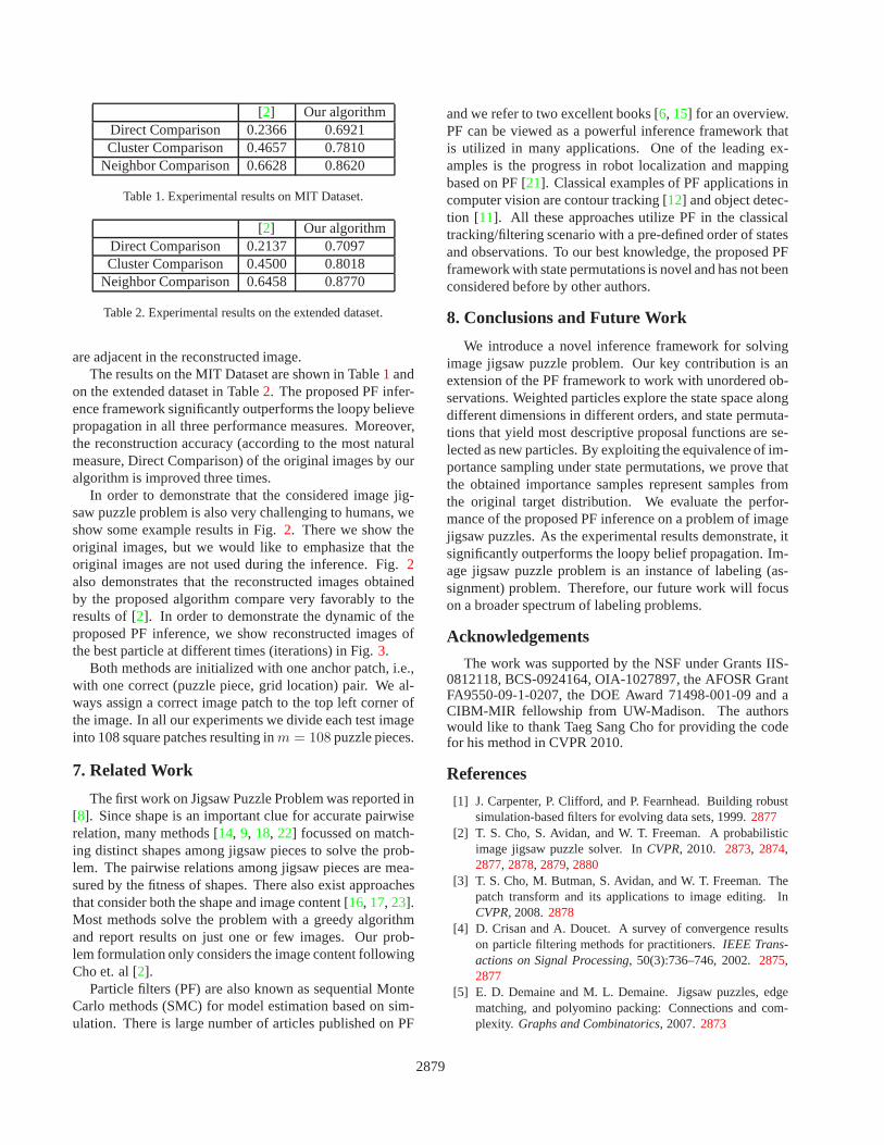
[2] Our algorithmDirect Comparison 0.2366 0.6921Cluster Comparison 0.4657 0.7810

Neighbor Comparison 0.6628 0.8620

Table 1. Experimental results on MIT Dataset.

[2] Our algorithmDirect Comparison 0.2137 0.7097Cluster Comparison 0.4500 0.8018

Neighbor Comparison 0.6458 0.8770

Table 2. Experimental results on the extended dataset.

are adjacent in the reconstructed image.The results on the MIT Dataset are shown in Table1 and

on the extended dataset in Table2. The proposed PF infer-ence framework significantly outperforms the loopy believepropagation in all three performance measures. Moreover,the reconstruction accuracy (according to the most naturalmeasure, Direct Comparison) of the original images by ouralgorithm is improved three times.

In order to demonstrate that the considered image jig-saw puzzle problem is also very challenging to humans, weshow some example results in Fig.2. There we show theoriginal images, but we would like to emphasize that theoriginal images are not used during the inference. Fig.2also demonstrates that the reconstructed images obtainedby the proposed algorithm compare very favorably to theresults of [2]. In order to demonstrate the dynamic of theproposed PF inference, we show reconstructed images ofthe best particle at different times (iterations) in Fig.3.

Both methods are initialized with one anchor patch, i.e.,with one correct (puzzle piece, grid location) pair. We al-ways assign a correct image patch to the top left corner ofthe image. In all our experiments we divide each test imageinto 108 square patches resulting inm = 108 puzzle pieces.

7. Related Work

The first work on Jigsaw Puzzle Problem was reported in[8]. Since shape is an important clue for accurate pairwiserelation, many methods [14, 9, 18, 22] focussed on match-ing distinct shapes among jigsaw pieces to solve the prob-lem. The pairwise relations among jigsaw pieces are mea-sured by the fitness of shapes. There also exist approachesthat consider both the shape and image content [16, 17, 23].Most methods solve the problem with a greedy algorithmand report results on just one or few images. Our prob-lem formulation only considers the image content followingCho et. al [2].

Particle filters (PF) are also known as sequential MonteCarlo methods (SMC) for model estimation based on sim-ulation. There is large number of articles published on PF

and we refer to two excellent books [6, 15] for an overview.PF can be viewed as a powerful inference framework thatis utilized in many applications. One of the leading ex-amples is the progress in robot localization and mappingbased on PF [21]. Classical examples of PF applications incomputer vision are contour tracking [12] and object detec-tion [11]. All these approaches utilize PF in the classicaltracking/filtering scenario with a pre-defined order of statesand observations. To our best knowledge, the proposed PFframework with state permutations is novel and has not beenconsidered before by other authors.

8. Conclusions and Future Work

We introduce a novel inference framework for solvingimage jigsaw puzzle problem. Our key contribution is anextension of the PF framework to work with unordered ob-servations. Weighted particles explore the state space alongdifferent dimensions in different orders, and state permuta-tions that yield most descriptive proposal functions are se-lected as new particles. By exploiting the equivalence of im-portance sampling under state permutations, we prove thatthe obtained importance samples represent samples fromthe original target distribution. We evaluate the perfor-mance of the proposed PF inference on a problem of imagejigsaw puzzles. As the experimental results demonstrate, itsignificantly outperforms the loopy belief propagation. Im-age jigsaw puzzle problem is an instance of labeling (as-signment) problem. Therefore, our future work will focuson a broader spectrum of labeling problems.

Acknowledgements

The work was supported by the NSF under Grants IIS-0812118, BCS-0924164, OIA-1027897, the AFOSR GrantFA9550-09-1-0207, the DOE Award 71498-001-09 and aCIBM-MIR fellowship from UW-Madison. The authorswould like to thank Taeg Sang Cho for providing the codefor his method in CVPR 2010.

References

[1] J. Carpenter, P. Clifford, and P. Fearnhead. Building robustsimulation-based filters for evolving data sets, 1999.2877

[2] T. S. Cho, S. Avidan, and W. T. Freeman. A probabilisticimage jigsaw puzzle solver. InCVPR, 2010. 2873, 2874,2877, 2878, 2879, 2880

[3] T. S. Cho, M. Butman, S. Avidan, and W. T. Freeman. Thepatch transform and its applications to image editing. InCVPR, 2008.2878

[4] D. Crisan and A. Doucet. A survey of convergence resultson particle filtering methods for practitioners.IEEE Trans-actions on Signal Processing, 50(3):736–746, 2002.2875,2877

[5] E. D. Demaine and M. L. Demaine. Jigsaw puzzles, edgematching, and polyomino packing: Connections and com-plexity. Graphs and Combinatorics, 2007.2873

2879

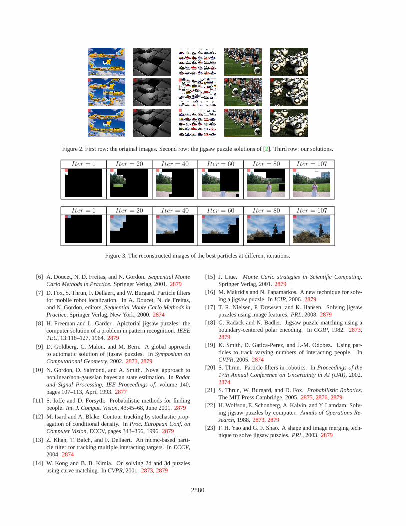
Figure 2. First row: the original images. Second row: the jigsaw puzzle solutions of [2]. Third row: our solutions.

Iter = 1 Iter = 20 Iter = 40 Iter = 60 Iter = 80 Iter = 107

Iter = 1 Iter = 20 Iter = 40 Iter = 60 Iter = 80 Iter = 107

Figure 3. The reconstructed images of the best particles at different iterations.

[6] A. Doucet, N. D. Freitas, and N. Gordon.Sequential MonteCarlo Methods in Practice. Springer Verlag, 2001.2879

[7] D. Fox, S. Thrun, F. Dellaert, and W. Burgard. Particle filtersfor mobile robot localization. In A. Doucet, N. de Freitas,and N. Gordon, editors,Sequential Monte Carlo Methods inPractice. Springer Verlag, New York, 2000.2874

[8] H. Freeman and L. Garder. Apictorial jigsaw puzzles: thecomputer solution of a problem in pattern recognition.IEEETEC, 13:118–127, 1964.2879

[9] D. Goldberg, C. Malon, and M. Bern. A global approachto automatic solution of jigsaw puzzles. InSymposium onComputational Geometry, 2002.2873, 2879

[10] N. Gordon, D. Salmond, and A. Smith. Novel approach tononlinear/non-gaussian bayesian state estimation. InRadarand Signal Processing, IEE Proceedings of, volume 140,pages 107–113, April 1993.2877

[11] S. Ioffe and D. Forsyth. Probabilistic methods for findingpeople.Int. J. Comput. Vision, 43:45–68, June 2001.2879

[12] M. Isard and A. Blake. Contour tracking by stochastic prop-agation of conditional density. InProc. European Conf. onComputer Vision, ECCV, pages 343–356, 1996.2879

[13] Z. Khan, T. Balch, and F. Dellaert. An mcmc-based parti-cle filter for tracking multiple interacting targets. InECCV,2004.2874

[14] W. Kong and B. B. Kimia. On solving 2d and 3d puzzlesusing curve matching. InCVPR, 2001.2873, 2879

[15] J. Liue. Monte Carlo strategies in Scientific Computing.Springer Verlag, 2001.2879

[16] M. Makridis and N. Papamarkos. A new technique for solv-ing a jigsaw puzzle. InICIP, 2006.2879

[17] T. R. Nielsen, P. Drewsen, and K. Hansen. Solving jigsawpuzzles using image features.PRL, 2008.2879

[18] G. Radack and N. Badler. Jigsaw puzzle matching using aboundary-centered polar encoding. InCGIP, 1982. 2873,2879

[19] K. Smith, D. Gatica-Perez, and J.-M. Odobez. Using par-ticles to track varying numbers of interacting people. InCVPR, 2005.2874

[20] S. Thrun. Particle filters in robotics. InProceedings of the17th Annual Conference on Uncertainty in AI (UAI), 2002.2874

[21] S. Thrun, W. Burgard, and D. Fox.Probabilistic Robotics.The MIT Press Cambridge, 2005.2875, 2876, 2879

[22] H. Wolfson, E. Schonberg, A. Kalvin, and Y. Lamdam. Solv-ing jigsaw puzzles by computer.Annals of Operations Re-search, 1988.2873, 2879

[23] F. H. Yao and G. F. Shao. A shape and image merging tech-nique to solve jigsaw puzzles.PRL, 2003.2879

2880