Embed Size (px)
Citation preview
Regression with Time Series
Part IX
Regression with Time Series
As of Oct 21, 2015Seppo Pynnonen Econometrics I
Regression with Time Series
Some Basic Concepts1 Regression with Time Series
Some Basic Concepts
Static Models
Finite Distributed Lag Model (FDL)
Multipliers
Testing for Significance of Long Run Propensity
Assumptions
Trends and Seasonality
Trending Variables in Regression
Seasonality
Time Series Models
Stationarity
Weakly Dependent Series
Basic Time Series Processes
Serial Correlation in Time Series Regression
Testing for Serial Correlation
Serial Correlation-Robust Inference with OLS
Estimating the residual autocorrelation as an AR-process
Residual Autocorrelation and Common Factor
Seppo Pynnonen Econometrics I
Regression with Time Series
Some Basic Concepts
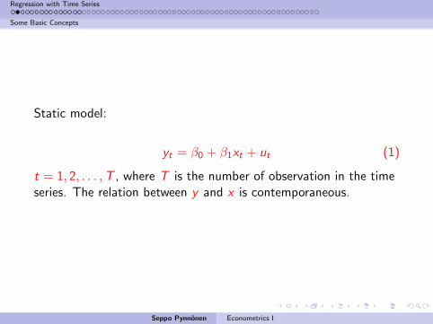
Static model:
yt = β0 + β1xt + ut (1)
t = 1, 2, . . . ,T , where T is the number of observation in the timeseries. The relation between y and x is contemporaneous.
Seppo Pynnonen Econometrics I
Regression with Time Series
Some Basic Concepts1 Regression with Time Series
Some Basic Concepts
Static Models
Finite Distributed Lag Model (FDL)
Multipliers
Testing for Significance of Long Run Propensity
Assumptions
Trends and Seasonality
Trending Variables in Regression
Seasonality
Time Series Models
Stationarity
Weakly Dependent Series
Basic Time Series Processes
Serial Correlation in Time Series Regression
Testing for Serial Correlation
Serial Correlation-Robust Inference with OLS
Estimating the residual autocorrelation as an AR-process
Residual Autocorrelation and Common Factor
Seppo Pynnonen Econometrics I
Regression with Time Series
Some Basic Concepts
Finite Distributed Lag Model (FDL):
In FDL models earlier values of one or more explanatory variablesaffect the current value of y .
yt = α0 + δ0xt + δ1xt−1 + δ2xt−2 + ut (2)
is a FDL of order two.
Interpretation of the coefficients?
Seppo Pynnonen Econometrics I
Regression with Time Series
Some Basic Concepts1 Regression with Time Series
Some Basic Concepts
Static Models
Finite Distributed Lag Model (FDL)
Multipliers
Testing for Significance of Long Run Propensity
Assumptions
Trends and Seasonality
Trending Variables in Regression
Seasonality
Time Series Models
Stationarity
Weakly Dependent Series
Basic Time Series Processes
Serial Correlation in Time Series Regression
Testing for Serial Correlation
Serial Correlation-Robust Inference with OLS
Estimating the residual autocorrelation as an AR-process
Residual Autocorrelation and Common Factor
Seppo Pynnonen Econometrics I

Regression with Time Series
Some Basic Concepts
Multipliers:
Multipliers indicate the impact of a unit change in x on y .
Impact Multiplier (Impact Propensity): Indicates the immediateone unit change in x on y . In (2) δ0 is the impact multiplier.
Seppo Pynnonen Econometrics I
Regression with Time Series
Some Basic Concepts
To see this, suppose xt is constant, say c , before time point t,increases by one unit to c + 1 at time point t and returns back toc at t + 1. That is
· · · , xt−2 = c , xt−1 = c , xt = c + 1, xt+1 = c , xt+2 = c , . . .
Seppo Pynnonen Econometrics I
Regression with Time Series
Some Basic Concepts
Suppose for the sake of simplicity that the error term is zero, then
yt−1 = α0 + δ0c + δ1c + δ2c
yt = α0 + δ0(c + 1) + δ1c + δ2c
yt+1 = α0 + δ0c + δ1(c + 1) + δ2c
yt+2 = α0 + δ0c + δ1c + δ2(c + 1)
yt+3 = α0 + δ0c + δ1c + δ2c
from which we findyt − yt−1 = δ0,
which is the immediate change in yt .
Seppo Pynnonen Econometrics I
Regression with Time Series
Some Basic Concepts
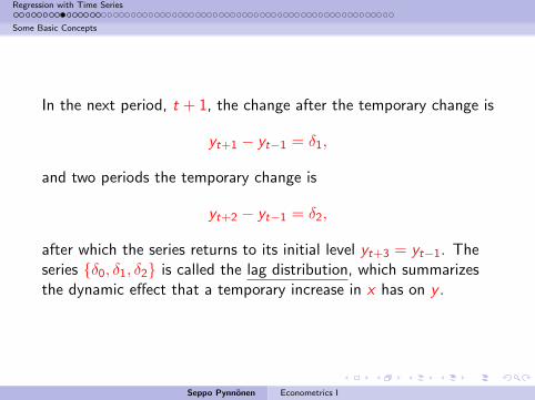
In the next period, t + 1, the change after the temporary change is
yt+1 − yt−1 = δ1,
and two periods the temporary change is
yt+2 − yt−1 = δ2,
after which the series returns to its initial level yt+3 = yt−1. Theseries δ0, δ1, δ2 is called the lag distribution, which summarizesthe dynamic effect that a temporary increase in x has on y .
Seppo Pynnonen Econometrics I
Regression with Time Series
Some Basic Concepts
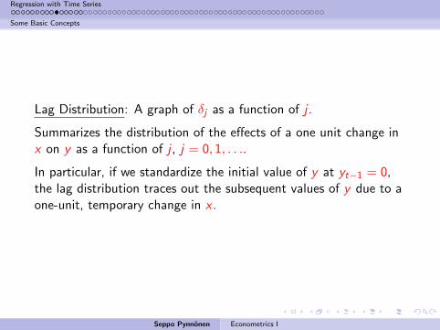
Lag Distribution: A graph of δj as a function of j .
Summarizes the distribution of the effects of a one unit change inx on y as a function of j , j = 0, 1, . . ..
In particular, if we standardize the initial value of y at yt−1 = 0,the lag distribution traces out the subsequent values of y due to aone-unit, temporary change in x .
Seppo Pynnonen Econometrics I
Regression with Time Series
Some Basic Concepts
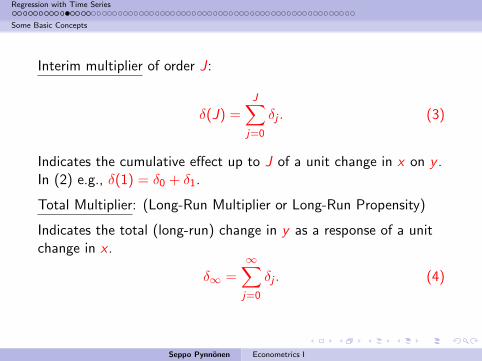
Interim multiplier of order J:
δ(J) =J∑
j=0
δj . (3)
Indicates the cumulative effect up to J of a unit change in x on y .In (2) e.g., δ(1) = δ0 + δ1.
Total Multiplier: (Long-Run Multiplier or Long-Run Propensity)
Indicates the total (long-run) change in y as a response of a unitchange in x .
δ∞ =∞∑j=0
δj . (4)
Seppo Pynnonen Econometrics I
Regression with Time Series
Some Basic Concepts
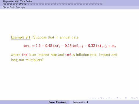
Example 9.1: Suppose that in annual data
intt = 1.6 + 0.48 inft − 0.15 inft−1 + 0.32 inft−2 + ut ,
where int is an interest rate and inf is inflation rate. Impact and
long-run multipliers?
Seppo Pynnonen Econometrics I
Regression with Time Series
Some Basic Concepts1 Regression with Time Series
Some Basic Concepts
Static Models
Finite Distributed Lag Model (FDL)
Multipliers
Testing for Significance of Long Run Propensity
Assumptions
Trends and Seasonality
Trending Variables in Regression
Seasonality
Time Series Models
Stationarity
Weakly Dependent Series
Basic Time Series Processes
Serial Correlation in Time Series Regression
Testing for Serial Correlation
Serial Correlation-Robust Inference with OLS
Estimating the residual autocorrelation as an AR-process
Residual Autocorrelation and Common Factor
Seppo Pynnonen Econometrics I
Regression with Time Series
Some Basic Concepts
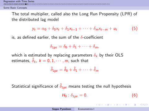
The total multiplier, called also the Long Run Propensity (LPR) ofthe distributed lag model
yt = α0 + δ0xt + δ1xt−1 + · · ·+ δmxt−m + ut (5)
is, as defined earlier, the sum of the δ-coefficient
δlpr = δ0 + δ1 + · · ·+ δm,
which is estimated by replacing parameters δk by their OLSestimates, δk , k = 0, 1, · · · ,m, such that
δlpr = δ0 + δ1 + · · ·+ δm
Statistical significance of δlpr means testing the null hypothesis
H0 : δlpr = 0. (6)
Seppo Pynnonen Econometrics I
Regression with Time Series
Some Basic Concepts
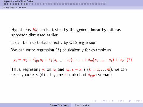
Hypothesis H0 can be tested by the general linear hypothesisapproach discussed earlier.
It can be also tested directly by OLS regression.
We can write regression (5) equivalently for example as
yt = α0 + δlprxt + δ1(xt−1 − xt) + · · ·+ δm(xt−m − xt) + ut . (7)
Thus, regressing yt on xt and xt−k − xt ’s (k = 1, . . .m), we cantest hypothesis (6) using the t-statistic of δlpr estimate.
Seppo Pynnonen Econometrics I
Regression with Time Series
Assumptions1 Regression with Time Series
Some Basic Concepts
Static Models
Finite Distributed Lag Model (FDL)
Multipliers
Testing for Significance of Long Run Propensity
Assumptions
Trends and Seasonality
Trending Variables in Regression
Seasonality
Time Series Models
Stationarity
Weakly Dependent Series
Basic Time Series Processes
Serial Correlation in Time Series Regression
Testing for Serial Correlation
Serial Correlation-Robust Inference with OLS
Estimating the residual autocorrelation as an AR-process
Residual Autocorrelation and Common Factor
Seppo Pynnonen Econometrics I
Regression with Time Series
Assumptions
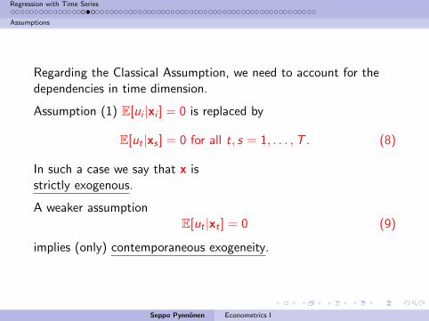
Regarding the Classical Assumption, we need to account for thedependencies in time dimension.
Assumption (1) E[ui |xi ] = 0 is replaced by
E[ut |xs ] = 0 for all t, s = 1, . . . ,T . (8)
In such a case we say that x isstrictly exogenous.
A weaker assumptionE[ut |xt ] = 0 (9)
implies (only) contemporaneous exogeneity.
Seppo Pynnonen Econometrics I
Regression with Time Series
Assumptions
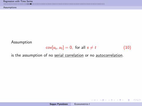
Assumptioncov[us , ut ] = 0, for all s 6= t (10)
is the assumption of no serial correlation or no autocorrelation.
Seppo Pynnonen Econometrics I
Regression with Time Series
Trends and Seasonality1 Regression with Time Series
Some Basic Concepts
Static Models
Finite Distributed Lag Model (FDL)
Multipliers
Testing for Significance of Long Run Propensity
Assumptions
Trends and Seasonality
Trending Variables in Regression
Seasonality
Time Series Models
Stationarity
Weakly Dependent Series
Basic Time Series Processes
Serial Correlation in Time Series Regression
Testing for Serial Correlation
Serial Correlation-Robust Inference with OLS
Estimating the residual autocorrelation as an AR-process
Residual Autocorrelation and Common Factor
Seppo Pynnonen Econometrics I
Regression with Time Series
Trends and Seasonality
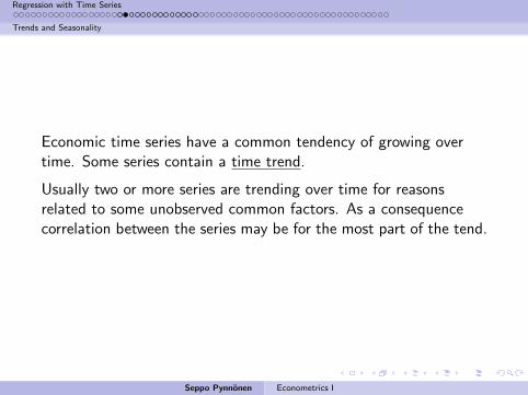
Economic time series have a common tendency of growing overtime. Some series contain a time trend.
Usually two or more series are trending over time for reasonsrelated to some unobserved common factors. As a consequencecorrelation between the series may be for the most part of the tend.
Seppo Pynnonen Econometrics I
Regression with Time Series
Trends and Seasonality
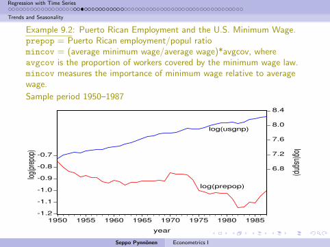
Example 9.2: Puerto Rican Employment and the U.S. Minimum Wage.prepop = Puerto Rican employment/popul ratiomincov = (average minimum wage/average wage)*avgcov, whereavgcov is the proportion of workers covered by the minimum wage law.mincov measures the importance of minimum wage relative to averagewage.
Sample period 1950–1987
-1.2
-1.1
-1.0
-0.9
-0.8
-0.7
6.8
7.2
7.6
8.0
8.4
1950 1955 1960 1965 1970 1975 1980 1985
year
log(usgnp)lo
g(pr
epop
)
log(usgnp)
log(prepop)
Seppo Pynnonen Econometrics I
Regression with Time Series
Trends and Seasonality
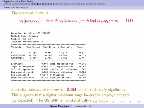
The specified model is
log(prepopt) = β0 + βi log(mincovt) + β2 log(usgnpt) + ut . (11)
Dependent Variable: LOG(PREPOP)
Method: Least Squares
Sample: 1950 1987
Included observations: 38
===========================================================
Variable Coefficient Std. Error t-Statistic Prob.
-----------------------------------------------------------
C -1.054 0.765 -1.378 0.177
LOG(MINCOV) -0.154 0.065 -2.380 0.023
LOG(USGNP) -0.012 0.089 -0.138 0.891
===========================================================
R-squared 0.660 Mean dependent var -0.944
Adjusted R-squared 0.641 S.D. dependent var 0.093
S.E. of regression 0.056 Akaike info criterion -2.862
Sum squared resid 0.109 Schwarz criterion -2.733
Log likelihood 57.376 F-statistic 34.043
Durbin-Watson stat 0.340 Prob(F-statistic) 0.000
===========================================================
Elasticity estimate of mincov is −0.154 and is statistically significant.
This suggests that a higher minimum wage lowers the employment rate
(as expected). The US GNP is not statistically significant.
Seppo Pynnonen Econometrics I
Regression with Time Series
Trends and Seasonality
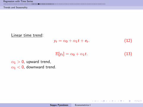
Linear time trend:yt = α0 + α1t + et . (12)
E[yt ] = α0 + α1t. (13)
α1 > 0, upward trend,α1 < 0, downward trend.
Seppo Pynnonen Econometrics I
Regression with Time Series
Trends and Seasonality
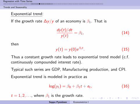
Exponential trend:
If the growth rate ∆y/y of an economy is β1. That is
dy(t)/dt
y(t)= β1, (14)
theny(t) = y(0)eβ1t . (15)
Thus a constant growth rate leads to exponential trend model (c.f.continuously compounded interest rate).
Typical such series are GDP, Manufacturing production, and CPI.
Exponential trend is modeled in practice as
log(yt) = β0 + β1t + et , (16)
t = 1, 2, . . ., where β1 is the growth rate.
Seppo Pynnonen Econometrics I
Regression with Time Series
Trends and Seasonality
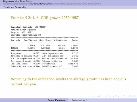
Example 9.3: U.S. GDP growth 1950–1987.
Dependent Variable: LOG(USGNP)
Method: Least Squares
Sample: 1950 1987
Included observations: 38
========================================================
Variable Coefficient Std. Error t-Statistic Prob.
--------------------------------------------------------
C 7.1549 0.012264 583.43 0.0000
@TREND 0.0304 0.000570 53.31 0.0000
========================================================
R-squared 0.987 Mean dependent var 7.717
Adjusted R-squared 0.987 S.D. dependent var 0.340
S.E. of regression 0.039 Akaike info criterion -3.623
Sum squared resid 0.053 Schwarz criterion -3.536
Log likelihood 70.830 F-statistic 2841.678
Durbin-Watson stat 0.446 Prob(F-statistic) 0.000
========================================================
According to the estimation results the average growth has been about 3
percent per year.
Seppo Pynnonen Econometrics I
Regression with Time Series
Trends and Seasonality1 Regression with Time Series
Some Basic Concepts
Static Models
Finite Distributed Lag Model (FDL)
Multipliers
Testing for Significance of Long Run Propensity
Assumptions
Trends and Seasonality
Trending Variables in Regression
Seasonality
Time Series Models
Stationarity
Weakly Dependent Series
Basic Time Series Processes
Serial Correlation in Time Series Regression
Testing for Serial Correlation
Serial Correlation-Robust Inference with OLS
Estimating the residual autocorrelation as an AR-process
Residual Autocorrelation and Common Factor
Seppo Pynnonen Econometrics I
Regression with Time Series
Trends and Seasonality
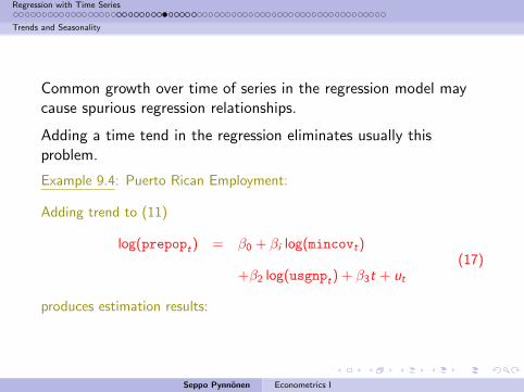
Common growth over time of series in the regression model maycause spurious regression relationships.
Adding a time tend in the regression eliminates usually thisproblem.
Example 9.4: Puerto Rican Employment:
Adding trend to (11)
log(prepopt) = β0 + βi log(mincovt)
+β2 log(usgnpt) + β3t + ut(17)
produces estimation results:
Seppo Pynnonen Econometrics I
Regression with Time Series
Trends and Seasonality
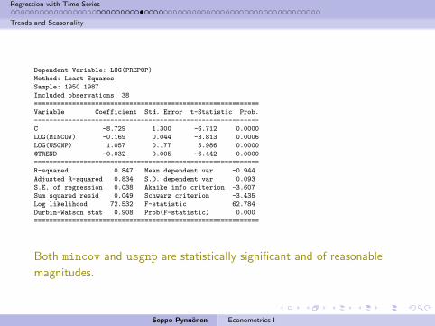
Dependent Variable: LOG(PREPOP)
Method: Least Squares
Sample: 1950 1987
Included observations: 38
===========================================================
Variable Coefficient Std. Error t-Statistic Prob.
-----------------------------------------------------------
C -8.729 1.300 -6.712 0.0000
LOG(MINCOV) -0.169 0.044 -3.813 0.0006
LOG(USGNP) 1.057 0.177 5.986 0.0000
@TREND -0.032 0.005 -6.442 0.0000
===========================================================
R-squared 0.847 Mean dependent var -0.944
Adjusted R-squared 0.834 S.D. dependent var 0.093
S.E. of regression 0.038 Akaike info criterion -3.607
Sum squared resid 0.049 Schwarz criterion -3.435
Log likelihood 72.532 F-statistic 62.784
Durbin-Watson stat 0.908 Prob(F-statistic) 0.000
===========================================================
Both mincov and usgnp are statistically significant and of reasonable
magnitudes.
Seppo Pynnonen Econometrics I
Regression with Time Series
Trends and Seasonality
Remark 9.1: Trend in dependent variable (y) may overstate R2.
To eliminate the effect, the R-square is better to compute by regressing
detrended y on x-variables and the trend (t).
Seppo Pynnonen Econometrics I
Regression with Time Series
Trends and Seasonality
Example 9.4b: (Example 9.4 continued)
Detrending log(prepop) and regressing it on the explanatory variables and
trend yields R2 = .533 ( compared to .834 in Ex 9.4).
Seppo Pynnonen Econometrics I
Regression with Time Series
Trends and Seasonality1 Regression with Time Series
Some Basic Concepts
Static Models
Finite Distributed Lag Model (FDL)
Multipliers
Testing for Significance of Long Run Propensity
Assumptions
Trends and Seasonality
Trending Variables in Regression
Seasonality
Time Series Models
Stationarity
Weakly Dependent Series
Basic Time Series Processes
Serial Correlation in Time Series Regression
Testing for Serial Correlation
Serial Correlation-Robust Inference with OLS
Estimating the residual autocorrelation as an AR-process
Residual Autocorrelation and Common Factor
Seppo Pynnonen Econometrics I
Regression with Time Series
Trends and Seasonality
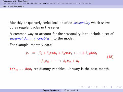
Monthly or quarterly series include often seasonality which showsup as regular cycles in the series.
A common way to account for the seasonality is to include a set ofseasonal dummy variables into the model.
For example, monthly data:
yt = β0 + δ1febt + δ2mart + · · ·+ δ11dect
+β1xt1 + · · ·+ βkxtk + ut(18)
febt , . . . , dect are dummy variables. January is the base month.
Seppo Pynnonen Econometrics I
Regression with Time Series
Time Series Models1 Regression with Time Series
Some Basic Concepts
Static Models
Finite Distributed Lag Model (FDL)
Multipliers
Testing for Significance of Long Run Propensity
Assumptions
Trends and Seasonality
Trending Variables in Regression
Seasonality
Time Series Models
Stationarity
Weakly Dependent Series
Basic Time Series Processes
Serial Correlation in Time Series Regression
Testing for Serial Correlation
Serial Correlation-Robust Inference with OLS
Estimating the residual autocorrelation as an AR-process
Residual Autocorrelation and Common Factor
Seppo Pynnonen Econometrics I
Regression with Time Series
Time Series Models
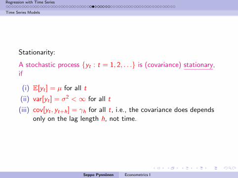
Stationarity:
A stochastic process yt : t = 1, 2, . . . is (covariance) stationary,if
(i) E[yt ] = µ for all t
(ii) var[yt ] = σ2 <∞ for all t
(iii) cov[yt , yt+h] = γh for all t, i.e., the covariance does dependsonly on the lag length h, not time.
Seppo Pynnonen Econometrics I
Regression with Time Series
Time Series Models1 Regression with Time Series
Some Basic Concepts
Static Models
Finite Distributed Lag Model (FDL)
Multipliers
Testing for Significance of Long Run Propensity
Assumptions
Trends and Seasonality
Trending Variables in Regression
Seasonality
Time Series Models
Stationarity
Weakly Dependent Series
Basic Time Series Processes
Serial Correlation in Time Series Regression
Testing for Serial Correlation
Serial Correlation-Robust Inference with OLS
Estimating the residual autocorrelation as an AR-process
Residual Autocorrelation and Common Factor
Seppo Pynnonen Econometrics I
Regression with Time Series
Time Series Models
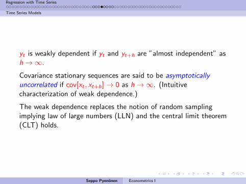
yt is weakly dependent if yt and yt+h are ”almost independent” ash→∞.
Covariance stationary sequences are said to be asymptoticallyuncorrelated if cov[xt , xt+h]→ 0 as h→∞. (Intuitivecharacterization of weak dependence.)
The weak dependence replaces the notion of random samplingimplying law of large numbers (LLN) and the central limit theorem(CLT) holds.
Seppo Pynnonen Econometrics I
Regression with Time Series
Time Series Models1 Regression with Time Series
Some Basic Concepts
Static Models
Finite Distributed Lag Model (FDL)
Multipliers
Testing for Significance of Long Run Propensity
Assumptions
Trends and Seasonality
Trending Variables in Regression
Seasonality
Time Series Models
Stationarity
Weakly Dependent Series
Basic Time Series Processes
Serial Correlation in Time Series Regression
Testing for Serial Correlation
Serial Correlation-Robust Inference with OLS
Estimating the residual autocorrelation as an AR-process
Residual Autocorrelation and Common Factor
Seppo Pynnonen Econometrics I
Regression with Time Series
Time Series Models
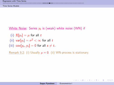
White Noise: Series yt is (weak) white noise (WN) if
(i) E[yt ] = µ for all t
(ii) var[yt ] = σ2 <∞ for all t
(iii) cov[ys , yt ] = 0 for all s 6= t.
Remark 9.2: (i) Usually µ = 0. (ii) WN-process is stationary.
Seppo Pynnonen Econometrics I
Regression with Time Series
Time Series Models
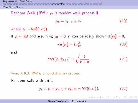
Random Walk (RW): yt is random walk process if
yt = yt−1 + et , (19)
where et ∼ WN(0, σ2e ).
If yt ∼ RW and assuming y0 = 0, it can be easily shown E[yt ] = 0,
var[yt ] = tσ2e , (20)
and
corr[yt , yt+h] =
√t
t + h. (21)
Remark 9.3: RW is a nonstationary process.
Random walk with drift:
yt = µ+ yt−1 + et , et ∼ WN(0, σ2e ). (22)
Seppo Pynnonen Econometrics I
Regression with Time Series
Time Series Models
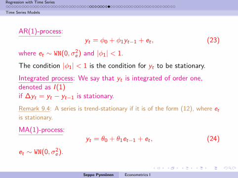
AR(1)-process:yt = φ0 + φ1yt−1 + et , (23)
where et ∼ WN(0, σ2e ) and |φ1| < 1.
The condition |φ1| < 1 is the condition for yt to be stationary.
Integrated process: We say that yt is integrated of order one,denoted as I (1)if ∆yt = yt − yt−1 is stationary.
Remark 9.4: A series is trend-stationary if it is of the form (12), where etis stationary.
MA(1)-process:yt = θ0 + θ1et−1 + et , (24)
et ∼ WN(0, σ2e ).
Seppo Pynnonen Econometrics I
Regression with Time Series
Serial Correlation in Time Series Regression1 Regression with Time Series
Some Basic Concepts
Static Models
Finite Distributed Lag Model (FDL)
Multipliers
Testing for Significance of Long Run Propensity
Assumptions
Trends and Seasonality
Trending Variables in Regression
Seasonality
Time Series Models
Stationarity
Weakly Dependent Series
Basic Time Series Processes
Serial Correlation in Time Series Regression
Testing for Serial Correlation
Serial Correlation-Robust Inference with OLS
Estimating the residual autocorrelation as an AR-process
Residual Autocorrelation and Common Factor
Seppo Pynnonen Econometrics I
Regression with Time Series
Serial Correlation in Time Series Regression
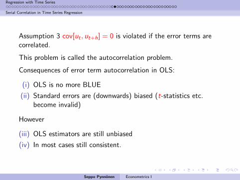
Assumption 3 cov[ut , ut+h] = 0 is violated if the error terms arecorrelated.
This problem is called the autocorrelation problem.
Consequences of error term autocorrelation in OLS:
(i) OLS is no more BLUE
(ii) Standard errors are (downwards) biased (t-statistics etc.become invalid)
However
(iii) OLS estimators are still unbiased
(iv) In most cases still consistent.
Seppo Pynnonen Econometrics I
Regression with Time Series
Serial Correlation in Time Series Regression1 Regression with Time Series
Some Basic Concepts
Static Models
Finite Distributed Lag Model (FDL)
Multipliers
Testing for Significance of Long Run Propensity
Assumptions
Trends and Seasonality
Trending Variables in Regression
Seasonality
Time Series Models
Stationarity
Weakly Dependent Series
Basic Time Series Processes
Serial Correlation in Time Series Regression
Testing for Serial Correlation
Serial Correlation-Robust Inference with OLS
Estimating the residual autocorrelation as an AR-process
Residual Autocorrelation and Common Factor
Seppo Pynnonen Econometrics I
Regression with Time Series
Serial Correlation in Time Series Regression
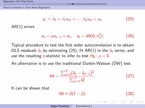
yt = β0 + β1xt1 + · · ·βkxtk + ut . (25)
AR(1) errors
ut = ρut−1 + et , et ∼ WN(0, σ2e ). (26)
Typical procedure to test the first order autocorrelation is to obtainOLS residuals ut by estimating (25), fit AR(1) in the ut series, anduse the resulting t-statistic to infer to test H0 : ρ = 0.
An alternative is to use the traditional Durbin-Watson (DW) test.
DW =
∑Tt=2(ut − ut−1)2∑T
t=1 u2t
. (27)
It can be shown thatDW ≈ 2(1− ρ). (28)
Seppo Pynnonen Econometrics I
Regression with Time Series
Serial Correlation in Time Series Regression
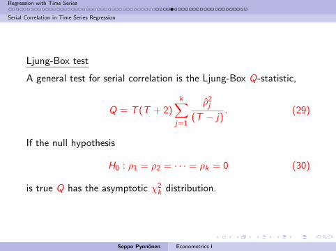
Ljung-Box test
A general test for serial correlation is the Ljung-Box Q-statistic,
Q = T (T + 2)k∑
j=1
ρ2j(T − j)
. (29)
If the null hypothesis
H0 : ρ1 = ρ2 = · · · = ρk = 0 (30)
is true Q has the asymptotic χ2k distribution.
Seppo Pynnonen Econometrics I
Regression with Time Series
Serial Correlation in Time Series Regression1 Regression with Time Series
Some Basic Concepts
Static Models
Finite Distributed Lag Model (FDL)
Multipliers
Testing for Significance of Long Run Propensity
Assumptions
Trends and Seasonality
Trending Variables in Regression
Seasonality
Time Series Models
Stationarity
Weakly Dependent Series
Basic Time Series Processes
Serial Correlation in Time Series Regression
Testing for Serial Correlation
Serial Correlation-Robust Inference with OLS
Estimating the residual autocorrelation as an AR-process
Residual Autocorrelation and Common Factor
Seppo Pynnonen Econometrics I
Regression with Time Series
Serial Correlation in Time Series Regression
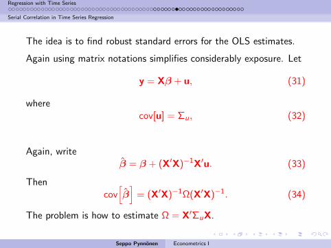
The idea is to find robust standard errors for the OLS estimates.
Again using matrix notations simplifies considerably exposure. Let
y = Xβ + u, (31)
wherecov[u] = Σu, (32)
Again, writeβ = β + (X′X)−1X′u. (33)
Thencov[β]
= (X′X)−1Ω(X′X)−1. (34)
The problem is how to estimate Ω = X′ΣuX.
Seppo Pynnonen Econometrics I
Regression with Time Series
Serial Correlation in Time Series Regression
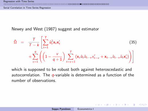
Newey and West (1987) suggest and estimator
Ω =T
T − k
[T∑t=1
u2t xtx′t (35)
+
q∑v=1
((1− v
q + 1
) T∑t=v+1
(xt ut ut−vx′t−v + xt−v ut−v utx
′t)
)]
which is supposed to be robust both against heteroscedastic andautocorrelation. The q-variable is determined as a function of thenumber of observations.
Seppo Pynnonen Econometrics I
Regression with Time Series
Serial Correlation in Time Series Regression
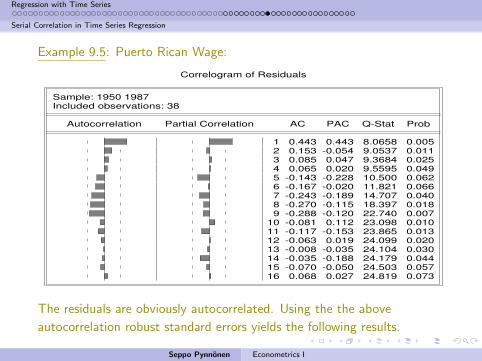
Example 9.5: Puerto Rican Wage:
Correlogram of Residuals
Sample: 1950 1987Included observations: 38
Autocorrelation Partial Correlation AC PAC Q-Stat Prob
1 0.443 0.443 8.0658 0.0052 0.153 -0.054 9.0537 0.0113 0.085 0.047 9.3684 0.0254 0.065 0.020 9.5595 0.0495 -0.143 -0.228 10.500 0.0626 -0.167 -0.020 11.821 0.0667 -0.243 -0.189 14.707 0.0408 -0.270 -0.115 18.397 0.0189 -0.288 -0.120 22.740 0.007
10 -0.081 0.112 23.098 0.01011 -0.117 -0.153 23.865 0.01312 -0.063 0.019 24.099 0.02013 -0.008 -0.035 24.104 0.03014 -0.035 -0.188 24.179 0.04415 -0.070 -0.050 24.503 0.05716 0.068 0.027 24.819 0.073
The residuals are obviously autocorrelated. Using the the above
autocorrelation robust standard errors yields the following results.
Seppo Pynnonen Econometrics I
Regression with Time Series
Serial Correlation in Time Series Regression
We observe that particularly the standard error of log(usgnb) increases
compared to Example 9.4.
Seppo Pynnonen Econometrics I
Regression with Time Series
Serial Correlation in Time Series Regression1 Regression with Time Series
Some Basic Concepts
Static Models
Finite Distributed Lag Model (FDL)
Multipliers
Testing for Significance of Long Run Propensity
Assumptions
Trends and Seasonality
Trending Variables in Regression
Seasonality
Time Series Models
Stationarity
Weakly Dependent Series
Basic Time Series Processes
Serial Correlation in Time Series Regression
Testing for Serial Correlation
Serial Correlation-Robust Inference with OLS
Estimating the residual autocorrelation as an AR-process
Residual Autocorrelation and Common Factor
Seppo Pynnonen Econometrics I
Regression with Time Series
Serial Correlation in Time Series Regression
An alternative to the robustifying of the standard errors with theNewy-White procedure (35), is to explicitly model the error termas an autoregressive process as is done in equation (26) andestimate it.
Seppo Pynnonen Econometrics I
Regression with Time Series
Serial Correlation in Time Series Regression
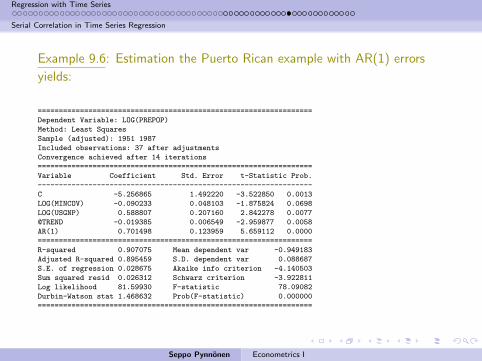
Example 9.6: Estimation the Puerto Rican example with AR(1) errors
yields:
=================================================================
Dependent Variable: LOG(PREPOP)
Method: Least Squares
Sample (adjusted): 1951 1987
Included observations: 37 after adjustments
Convergence achieved after 14 iterations
=================================================================
Variable Coefficient Std. Error t-Statistic Prob.
-----------------------------------------------------------------
C -5.256865 1.492220 -3.522850 0.0013
LOG(MINCOV) -0.090233 0.048103 -1.875824 0.0698
LOG(USGNP) 0.588807 0.207160 2.842278 0.0077
@TREND -0.019385 0.006549 -2.959877 0.0058
AR(1) 0.701498 0.123959 5.659112 0.0000
=================================================================
R-squared 0.907075 Mean dependent var -0.949183
Adjusted R-squared 0.895459 S.D. dependent var 0.088687
S.E. of regression 0.028675 Akaike info criterion -4.140503
Sum squared resid 0.026312 Schwarz criterion -3.922811
Log likelihood 81.59930 F-statistic 78.09082
Durbin-Watson stat 1.468632 Prob(F-statistic) 0.000000
=================================================================
Seppo Pynnonen Econometrics I
Regression with Time Series
Serial Correlation in Time Series Regression
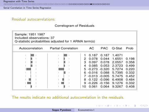
Residual autocorrelations:
Correlogram of Residuals
Sample: 1951 1987Included observations: 37Q-statistic probabilities adjusted for 1 ARMA term(s)
Autocorrelation Partial Correlation AC PAC Q-Stat Prob
1 0.187 0.187 1.40712 0.078 0.044 1.6551 0.1983 0.097 0.078 2.0557 0.3584 0.085 0.053 2.3723 0.4995 -0.273 -0.320 5.7274 0.2206 -0.016 0.088 5.7395 0.3327 -0.013 -0.005 5.7475 0.4528 -0.122 -0.096 6.4908 0.4849 -0.226 -0.156 9.1276 0.332
10 0.061 0.064 9.3267 0.408
The results indicate no additional autocorrelation in the residuals.
Seppo Pynnonen Econometrics I
Regression with Time Series
Serial Correlation in Time Series Regression1 Regression with Time Series
Some Basic Concepts
Static Models
Finite Distributed Lag Model (FDL)
Multipliers
Testing for Significance of Long Run Propensity
Assumptions
Trends and Seasonality
Trending Variables in Regression
Seasonality
Time Series Models
Stationarity
Weakly Dependent Series
Basic Time Series Processes
Serial Correlation in Time Series Regression
Testing for Serial Correlation
Serial Correlation-Robust Inference with OLS
Estimating the residual autocorrelation as an AR-process
Residual Autocorrelation and Common Factor
Seppo Pynnonen Econometrics I
Regression with Time Series
Serial Correlation in Time Series Regression
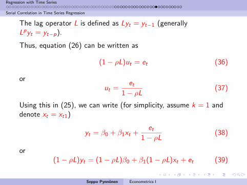
The lag operator L is defined as Lyt = yt−1 (generallyLpyt = yt−p).
Thus, equation (26) can be written as
(1− ρL)ut = et (36)
orut =
et1− ρL
(37)
Using this in (25), we can write (for simplicity, assume k = 1 anddenote xt = xt1)
yt = β0 + β1xt +et
1− ρL(38)
or(1− ρL)yt = (1− ρL)β0 + β1(1− ρL)xt + et (39)
Seppo Pynnonen Econometrics I
Regression with Time Series
Serial Correlation in Time Series Regression
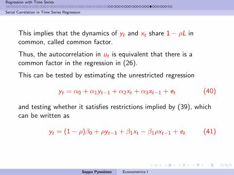
This implies that the dynamics of yt and xt share 1− ρL incommon, called common factor.
Thus, the autocorrelation in ut is equivalent that there is acommon factor in the regression in (26).
This can be tested by estimating the unrestricted regression
yt = α0 + α1yt−1 + α2xt + α3xt−1 + et (40)
and testing whether it satisfies restrictions implied by (39), whichcan be written as
yt = (1− ρ)β0 + ρyt−1 + β1xt − β1ρxt−1 + et (41)
Seppo Pynnonen Econometrics I
Regression with Time Series
Serial Correlation in Time Series Regression
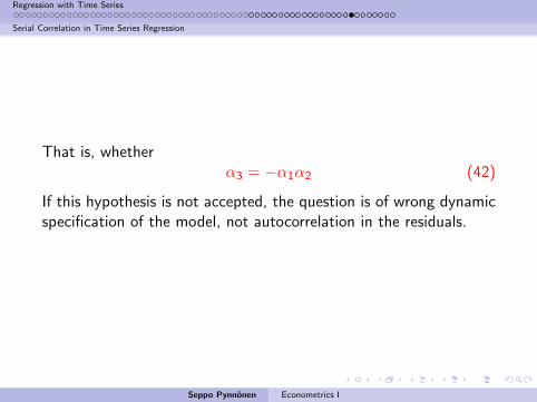
That is, whetherα3 = −α1α2 (42)
If this hypothesis is not accepted, the question is of wrong dynamicspecification of the model, not autocorrelation in the residuals.
Seppo Pynnonen Econometrics I
Regression with Time Series
Serial Correlation in Time Series Regression
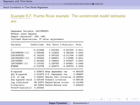
Example 9.7: Puerto Rican example. The unrestricted model estimates
are:
Dependent Variable: LOG(PREPOP)
Method: Least Squares
Sample (adjusted): 1951 1987
Included observations: 37 after adjustments
===========================================================
Variable Coefficient Std. Error t-Statistic Prob.
-----------------------------------------------------------
C -5.612596 1.547354 -3.627223 0.0011
LOG(PREPOP(-1)) 0.535366 0.124932 4.285246 0.0002
LOG(MINCOV) -0.142230 0.047224 -3.011794 0.0052
LOG(MINCOV(-1)) 0.033409 0.046831 0.713386 0.4811
LOG(USGNP) 0.561893 0.188654 2.978437 0.0057
LOG(USGNP(-1)) 0.137353 0.226785 0.605651 0.5493
@TREND -0.019768 0.005975 -3.308752 0.0024
===========================================================
R-squared 0.928815 Mean dependent var -0.949183
Adj R-squared 0.914578 S.D. dependent var 0.088687
S.E. of reg 0.025921 Akaike info criterion -4.298904
Sum squared resid 0.020156 Schwarz criterion -3.994136
Log likelihood 86.52972 Hannan-Quinn criter. -4.191459
F-statistic 65.23934 Durbin-Watson stat 1.634219
Prob(F-statistic) 0.000000
===========================================================
Seppo Pynnonen Econometrics I
Regression with Time Series
Serial Correlation in Time Series Regression
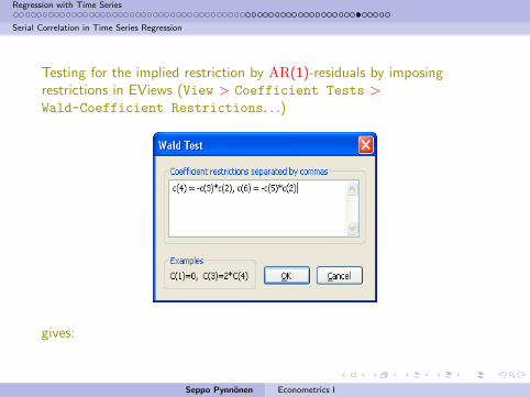
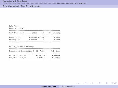
Testing for the implied restriction by AR(1)-residuals by imposingrestrictions in EViews (View > Coefficient Tests >Wald-Coefficient Restrictions. . .)
gives:
Seppo Pynnonen Econometrics I
Regression with Time Series
Serial Correlation in Time Series Regression
Wald Test:
Equation: EX97
=================================================
Test Statistic Value df Probability
-------------------------------------------------
F-statistic 4.436898 (2, 30) 0.0205
Chi-square 8.873795 2 0.0118
=================================================
Null Hypothesis Summary:
=================================================
Normalized Restriction (= 0) Value Std. Err.
-------------------------------------------------
C(2)*C(3) + C(4) -0.042736 0.033279
C(2)*C(5) + C(6) 0.438171 0.150355
=================================================
Seppo Pynnonen Econometrics I
Regression with Time Series
Serial Correlation in Time Series Regression
The null hypothesis is rejected, which implies that rather than the errorterm is autocorrelated the model should be specified as
yt = β0 + α1yt−1 + β1xt1 + β11xt−1,1 + β2xt,2 + β21xt−1,2 + et ,
where y = log(prepop), x1 = log(mincov), x2 = log(usgnp), and
x3 = trend.
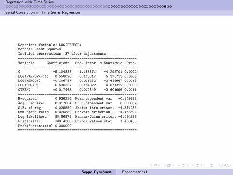
Finally, because the coefficient estimates of log(mincovt−1) and
log(usgnpt−1) are not statistically significant, they can be dropped from
the model. So the final model becomes:
Seppo Pynnonen Econometrics I
Regression with Time Series
Serial Correlation in Time Series Regression
Dependent Variable: LOG(PREPOP)
Method: Least Squares
Included observations: 37 after adjustments
==========================================================
Variable Coefficient Std. Error t-Statistic Prob.
----------------------------------------------------------
C -5.104888 1.188371 -4.295701 0.0002
LOG(PREPOP(-1)) 0.558090 0.103817 5.375713 0.0000
LOG(MINCOV) -0.106787 0.031282 -3.413647 0.0018
LOG(USGNP) 0.630332 0.154822 4.071322 0.0003
@TREND -0.017463 0.004849 -3.601696 0.0011
==========================================================
R-squared 0.926226 Mean dependent var -0.949183
Adj R-squared 0.917004 S.D. dependent var 0.088687
S.E. of reg 0.025550 Akaike info criter. -4.371286
Sum sqerd resid 0.020889 Schwarz criterion -4.153594
Log likelihood 85.86878 Hannan-Quinn criter. -4.294539
F-statistic 100.4388 Durbin-Watson stat 1.468436
Prob(F-statistic) 0.000000
==========================================================
Seppo Pynnonen Econometrics I
Regression with Time Series
Serial Correlation in Time Series Regression
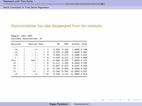
Autocorrelation has also disappeared from the residuals:
Sample: 1951 1987
Included observations: 37
=============================================================
Autocorr Partial Corr AC PAC Q-Stat Prob
-------------------------------------------------------------
. |*. | . |*. | 1 0.203 0.203 1.6465 0.199
. |*. | . | . | 2 0.079 0.039 1.9008 0.387
. |*. | . | . | 3 0.092 0.072 2.2586 0.521
. | . | . | . | 4 0.018 -0.017 2.2724 0.686
***| . | ***| . | 5 -0.346 -0.372 7.6823 0.175
.*| . | . | . | 6 -0.111 0.020 8.2560 0.220
.*| . | . | . | 7 -0.067 -0.010 8.4747 0.293
.*| . | . | . | 8 -0.124 -0.052 9.2354 0.323
.*| . | .*| . | 9 -0.143 -0.091 10.2920 0.327
. |*. | . |*. | 10 0.156 0.110 11.5860 0.314
=============================================================
Seppo Pynnonen Econometrics I

Regression with Time Series
Serial Correlation in Time Series Regression
End of Notes
Seppo Pynnonen Econometrics I


![ANTHROPOLOGICAL MISCELLANEA.ANTHROPOLOGICAL MISCELLANEA. REGRESSION towards MEDIOCRITY in HEREDITARY STATURE. By FRANCIS GALTON, F.R.S. &C. [WITH PLATES IX AND X.] THIS memoir contains](https://img.dokumen.tips/doc/110x75/60c74c6227c11f358e06c7f2/anthropological-anthropological-miscellanea-regression-towards-mediocrity-in.jpg)