Embed Size (px)
Citation preview
PARAMETER ESTIMATION FOR HIDDEN MARKOVMODELS WITH INTRACTABLE LIKELIHOODS
By Thomas. A. Dean1,∗, Sumeetpal S. Singh1,∗, AjayJasra and Gareth w. Peters
University of Cambridge1, Imperial College London and University of NewSouth Wales
Approximate Bayesian computation (ABC) is a popular tech-nique for approximating likelihoods and is often used in parameterestimation when the likelihood functions are analytically intractable.Although the use of ABC is widespread in many fields, there has beenlittle investigation of the theoretical properties of the resulting esti-mators. In this paper we give a theoretical analysis of the asymptoticproperties of ABC based maximum likelihood parameter estimationfor hidden Markov models. In particular, we derive results analogousto those of consistency and asymptotic normality for standard max-imum likelihood estimation. We also discuss how Sequential MonteCarlo methods provide a natural method for implementing likelihoodbased ABC procedures.
1. Introduction. The hidden Markov model (HMM) is an importantstatistical model in many fields including Bioinformatics (e.g. Durbin et al.(1998)), Econometrics (e.g. Kim, Shephard and Chib (1998)) and Popula-tion genetics (e.g. Felsenstein and Churchill (1996)); see also Cappe, Rydenand Moulines (2005) for a recent overview. Often one has a range of HMMsparameterised by a parameter vector θ taking values in some compact sub-set Θ of Euclidian space. Given a sequence of observations Y1, . . . , Yn theobjective is to find the parameter vector θ∗ ∈ Θ that corresponds to theparticular HMM from which the data were generated.
A common approach to estimating θ∗ is maximum likelihood estimation(MLE). The parameter estimate, denoted θn, is obtained via maximizing
∗T.A. Dean and S.S. Singh’s research is funded by the Engineering and Physical Sci-ences Research Council (EP/G037590/1) whose support is gratefully acknowledged. This
AMS 2000 subject classifications: Primary 62M09; secondary 62B99, 62F12, 65C05Keywords and phrases: Parameter Estimation, Hidden Markov Model, Maximum Like-
lihood, Approximate Bayesian Computation, Sequential Monte CarloFirst version: Cambridge University Engineering Department Technical Report 660, 1
October 2010
1
arX
iv:1
103.
5399
v1 [
mat
h.ST
] 2
8 M
ar 2
011
2 DEAN ET AL.
the log-likelihood of the observations:
θn = arg maxθ∈Θln(θ)
where
ln(θ) := log pθ
(Y1, . . . , Yn
)=
n∑i=1
log pθ(Yi|Y1, . . . , Yi−1).
Unless the model is simple, e.g. linear Gaussian or when X is a finite set,one can seldom evaluate the likelihood analytically. There are a variety oftechniques, for example sequential Monte Carlo (SMC), for numerically esti-mating the likelihood. However, in a wide range of applications these meth-ods cannot be used, for example when the conditional density of the ob-served state of the HMM given the hidden state is intractable, by which wemean that this density cannot be evaluated analytically and has no unbiasedMonte Carlo estimator. Despite this, one is often still able to generate sam-ples from the corresponding processes for different values of the parameterθ (e.g. Jasra et al. (2010)). This has led to the development of methods inwhich θ∗ is estimated by taking the value of θ which maximizes some prin-cipled approximation of the likelihood which is itself estimated using MonteCarlo simulation.
One such approach is the convolution particle filter of Campillo and Rossi(2009). Another technique which can be applied to this class of problems isindirect inference; see Gourieroux, Monfort and Renault (1993) and Hegg-land and Frigessi (2004). However in the context of HMMs, when one doesnot adopt a linear Gaussian approximation of the filtering density (whichcan be very inaccurate, as in extended Kalman filter approximations), thismethod is likely to be very expensive. A third method which has recentlyreceived a great deal of attention is approximate Bayesian computation(ABC). A non-exhaustive list of references includes: McKinley, Cook andDeardon (2009); Peters, Wuthrich and Shevchenko (2010); Pritchard et al.(1999); Ratmann et al. (2009); Tavre et al. (1997). See also Sisson and Fan(to be published) for a review on computational methodology.
In the standard ABC approach (omitting for the moment the possible useof summary statistics) one assumes that a data set Y1, . . . , Yn is given and
approximates the likelihood function pθ
(Y1, . . . , Yn
)via probabilities of the
form
(1) Pθ(d(Y1, . . . , Yn; Y1, . . . , Yn
)≤ ε)
where {Yk}k≥1 denotes the observed state of the HMM, d(·; ·) is some suit-able metric on the n-fold product space Rm × · · · × Rm and ε > 0 is a
ESTIMATION OF INTRACTABLE HMMS 3
constant which reflects the accuracy of the approximation. In practice theseprobabilities are themselves estimated using Monte Carlo techniques.
The intuitive justification for the ABC approximation is that for suffi-ciently small ε
Pθ(d(Y1, . . . , Yn; Y1, . . . , Yn
)≤ ε)
V εY1,...,Yn
≈ pθ(Y1, . . . , Yn
)where V ε
Y1,...,Yndenotes the volume of the d-ball of radius ε around the points
Y1, . . . , Yn. Thus the probabilities (1) will provide a good approximationto the likelihood, up to the value of some renormalising factor which isindependent of θ and hence can be ignored. However in general it is not atall clear in what sense an approximation to the likelihood must be ‘good’ inorder for the resulting inference procedures to be well behaved. The purposeof this paper is to resolve this issue by directly investigating the effect ofthe parameter ε, not on the quality of the approximations (1), but on thebehaviour of the resulting ABC based parameter estimators.
We note that in (1) we have implicitly assumed that one is working withthe entire data set rather than a summary statistic of it as is usually donein practice, especially when the observations {Yk}k≥0 take values in somehigh dimensional space. For ease of exposition we shall persist with thisassumption throughout the rest of the paper, noting where appropriate theconditions under which the results we derive will continue to hold whensummary statistics are used (see in particular the remarks at the ends ofSections 3 and 4).
1.1. Contribution and Structure. In this paper we investigate the be-haviour of ABC when used to estimate the parameters of HMMs for whichthe conditional densities of the observations given the hidden state are in-tractable. We shall use a specialization, first proposed in Jasra et al. (2010),of the standard ABC likelihood approximation (1) for when the observationsare generated by a HMM. Specifically we approximate the likelihood of agiven sequence of observations Y1, . . . , Yn from a HMM with the probability
(2) Pθ(Y1 ∈ Bε
Y1, . . . , Yn ∈ Bε
Yn
)where Bε
y denotes the ball of radius ε centered around the point y. Thebenefit of this approach is that it retains the Markovian structure of themodel. This facilitates both simpler Markov chain Monte Carlo (MCMC)(e.g. McKinley, Cook and Deardon (2009)) and sequential Monte Carlo
4 DEAN ET AL.
(SMC) (e.g. Jasra et al. (2010)) implementation of the ABC approximation.Furthermore our experience suggests that this approximation is competitive,from an accuracy perspective, with a wide range of competing methods; seethe two afore mentioned references for a deeper discussion of this point.
One could use the approximate likelihoods (2) to estimate the parametersof a HMM in one of two ways. Firstly one could take a Bayesian approachand use (2) to construct an approximation to the posterior. This is the ap-proach most commonly taken in the literature. Alternatively, as we shall doin this paper, one could take a frequentist approach and estimate the param-eters of the HMM with the value of the parameter vector which maximizesthe corresponding approximate likelihood (2) of the observations. We shallhenceforth term this procedure approximate Bayesian computation maxi-mum likelihood estimation (ABC MLE).
Although the use of ABC has become commonplace there has to datebeen little investigation of the theoretical properties of its use in parameterestimation in either the Bayesian or frequentist context. In particular thefollowing questions remain to be answered. Is ABC MLE consistent? DoABC based posterior distributions concentrate around the true value of theparameter vector? Indeed do ABC based estimators converge to anything atall? Although these questions may seem abstract it is well known that eventhe mighty MLE can fail to converge in practice, see Ferguson (1982). Thusbefore ABC can be placed on firm mathematical foundations the questionsraised above need to be addressed.
The purpose of this paper is to bridge this theoretical gap in the context ofmaximum likelihood estimation. In particular we develop a theoretical jus-tification of the ABC MLE procedure based on its large sample propertiesanalogous to that provided for MLE by standard results concerning asymp-totic consistency and normality. Our approach to this problem is based onthe novel observation that ABC MLE can be considered as performing MLEusing the likelihoods of a collection of perturbed HMMs. This implies thatthe ABC MLE should in some sense inherit its behaviour from the standardMLE. Using this observation we first show that unlike the MLE, which isasymptotically consistent, the ABC MLE estimator has an innate asymp-totic bias. Secondly we show that this bias can be made arbitrarily smallby choosing sufficiently small values of ε. Together these results show thatasymptotically the ABC MLE will converge to the true parameter value witha margin of error which can be made arbitrarily small by taking a suitablechoice of ε. Thus our results allow us to develop a rigorous formulation of theintuitive justification of ABC and in doing so to provide a firm mathematicalbasis for performing ABC based inference.
ESTIMATION OF INTRACTABLE HMMS 5
We complete the picture by analysing the so called noisy variant (seee.g. Fearnhead and Prangle (2010)) of ABC MLE. We show that unlikethe ABC MLE the noisy ABC MLE is always asymptotically consistent.This raises the question: does noisy ABC provide us with a ‘free pass’ whenperforming parameter estimation? Unfortunately the answer in general isno. We show that under reasonable conditions the Fisher information of thenoisy ABC MLE is strictly less than that of the standard MLE. As a resultwe show that the noisy ABC suffers from a relative loss of information andhence statistical efficiency.
As part of these investigations we establish a novel asymptotic missinginformation principle for HMMs with observations perturbed by additiveuniform noise which may in itself be of independent interest to the reader.Finally we remark that although this study is theoretical it is our belief thatthe results presented herein will help provide guidance for future method-ological developments in the field.
This paper is structured as follows. In Section 2 the notation and assump-tions are given. In Section 3 we establish some approximate asymptoticconsistency type results for the standard ABC MLE. In Section 4 resultsconcerning the asymptotic consistency and normality of the noisy ABC es-timator are presented. An extension of the ABC method using probabilitykernels is discussed in Section 5 and an overview of the use of SMC methodsto provide a practical way of implementing ABC is presented in Section 6.An example is given in Section 7 which provides a qualitative demonstrationof the behaviour of the ABC estimator predicted in Sections 3 and 4. Thearticle is summarized in Section 8. Supporting technical lemmas and proofsof some of the theoretical results are housed in the two appendices.
2. Notation and Assumptions.
2.1. Notation and Main Assumptions. Throughout this paper we shalluse lower case letters x, y, z to denote dummy variables and upper case lettersX,Y, Z to denote random variables. Observations of a random variable willbe denoted by Y .
We shall frequently have to refer to various kinds of both finite, infiniteand doubly infinite sequences. For brevity the following shorthand nota-tions are used. For any pair of integers k ≤ n, Yk:n denotes the sequence ofrandom variables Yk, . . . , Yn; Y−∞:k denotes the sequence . . . , Yk; Yn:∞ de-notes the sequence Yn, . . . and Y−∞:k;n:∞ denotes the sequence . . . , Yk;Yn, . . ..Given a sequence of integers . . . , j−1, j0, j1, . . . and indicies r < s we shalllet jr:s denote jr, jr+1, . . . , js−1, js; j−∞:r denote . . . , jr−1, jr and js:∞ de-note js, js+1, . . . respectively. Further we shall also use j−∞:∞ to denote
6 DEAN ET AL.
the full sequence . . . , j−1, j0, j1, . . .. The two notations defined above willbe combined in the following manner. Given a doubly infinite sequence ofrandom variables . . . , Y−1, Y0, Y1, . . ., a doubly infinite sequence of integers. . . , j−1, j0, j1, . . . and indicies r < s we shall let Yjr:s denote the sequenceYjr , Yjr+1 , . . . , Yjs−1 , Yjs . The sequences Yj−∞:r , Yjs:∞ and Yj−∞:∞ are definedanalogously. Lastly given a measure µ on a Polish space X we let
∫·µ(dx1:n)
denote integration w.r.t. the n-fold product measure µ⊗n on the n-fold prod-uct space X n. Moreover, given a function f(x1, . . . , xn) : X n → R and in-tegers 1 ≤ k ≤ l ≤ n, we shall let
∫Xn f(·)µ(dx1:k;l:n) denote the partial
integrals∫Xn f(·)µ(dx1) · · ·µ(dxk)µ(dxl) · · ·µ(dxn).
The essence of our approach is to show that in some sense the ABCMLE inherits the properties of the standard MLE. Thus we shall operateunder assumptions on the HMMs that are sufficient to ensure asymptoticconsistency and normality of the MLE.
It is assumed that the Markov chain {Xk}k≥0 is time-homogenous andtakes values in a compact Polish space X with associated Borel σ-field B (X ).Throughout it will be assumed that we have a collection of HMMs all definedon the same state space and parametrised by some vector θ taking values ina compact set Θ ∈ Rd. Furthermore we shall reserve θ∗ to denote the ‘true’value of the parameter vector. For each θ ∈ Θ we let Qθ (x, ·) denote thetransition kernel of the corresponding Markov chain and for each x ∈ X andθ ∈ Θ we assume that Qθ (x, ·) has a density qθ (x, ·) w.r.t. some commonfinite dominating measure µ on X . The initial distribution of the hiddenstate will be denoted by π0.
We also assume that the observations {Yk}k≥0 take values in a statespace Y ⊂ Rm for some m ≥ 1. Furthermore, for each k we assume thatthe random variable Yk is conditionally independent of X−∞:k−1;k+1:∞ andY−∞:k−1;k+1:∞ given Xk and that the conditional laws have densities gθ (y|x)w.r.t. some common finite dominating measure ν. We further assume thatfor every θ the joint chain {Xk, Yk}k≥0 is positive Harris recurrent and has
a unique invariant distribution πθ. We shall write Pθ to denote the laws ofthe corresponding stationary processes and Eθ to denote expectations withrespect to the stationary laws Pθ.
Given any ε > 0 and y ∈ Rm let Bεy denote the closed ball of radius ε
centered on the point y and let UBεy denote the uniform distribution on Bεy.
For any A ⊂ Rm, let IA denote the indicator function of A. Additionally,for any square matrix M ∈ Rm×m, we shall let ‖M‖ denote the Frobeniusnorm ‖M‖2 =
∑mj,k=1M
2j,k.
For any two probability measures µ1, µ2 on a measurable space (E,E ) welet ‖µ1 − µ2‖TV denote the total variation distance between them. For all
ESTIMATION OF INTRACTABLE HMMS 7
p ∈ [1,∞) we let Lp(µ) denote the set of real valued measurable functionssatisfying
∫|f(x)|p µ(dx) <∞.
Finally, we note that the asymptotic results that we prove for the ABCMLE and its noisy variant hold independently of the initial condition of thehidden state process {Xk}k≥0. Thus, in order to keep the presentation asconcise as possible we shall suppress the presence of the initial condition ofthe hidden state except in those instances where it needs to be referred toexplicitly.
2.2. Particular Assumptions. In addition to the assumptions above, thefollowing assumptions are made at various points in the article. Assump-tions (A1)-(A3) below are sufficient to guarantee asymptotic consistencyof the MLE and (A4)-(A5) ensure the existence of an asymptotic Fisherinformation matrix, denoted I(θ∗). Further, if the asymptotic Fisher infor-mation I(θ∗) is invertible then under assumptions (A1)-(A5) the MLE willbe asymptotically normal, see Douc, Moulines and Ryden (2004) for moredetails.
(A1) The parameter vector θ∗ belongs to the interior of Θ and θ = θ∗ if andonly if Pθ(. . . , Y−1, Y0, Y1, . . .) = Pθ∗(. . . , Y−1, Y0, Y1, . . .).
(A2) For all y ∈ Y, x, x′ ∈ X , the mappings θ → qθ(x, x′) and θ → gθ(y|x)
are continuous w.r.t. θ.
(A3) There exist constants c1, c1 ∈ (0,∞) such that for every y ∈ Y, x, x′ ∈X , θ ∈ Θ
c1 ≤ qθ(x, x′), gθ(y|x) ≤ c1.
For the remaining assumptions we assume that there exists an open ballG ⊂ Θ centered at θ∗ such that
(A4) For all y ∈ Y, x, x′ ∈ X , the mappings θ → qθ(x, x′) and θ → gθ(y|x)
are twice continuously differentiable on G.
(A5) There exists a constant c2 ∈ (0,∞) such that for every y ∈ Y, x, x′ ∈X , θ ∈ G ∣∣∇θ log qθ(x, x
′)∣∣ , |∇θ log gθ (y|x)| , |∇2
θ log qθ(x, x′)|,
|∇2θ log gθ (y|x) | ≤ c2.
Remark 1. In general assumptions (A3) and (A5) hold when the statespace X is compact and when the conditional laws of the observed state giventhe hidden state are heavy tailed, see for example Section 7. However weexpect that the behaviours predicted by Theorems 1, 2, 3 and 5 will provide
8 DEAN ET AL.
a good qualitative guide to the behaviour of ABC MLE in practice even incases where the underlying HMMs do not satisfy these assumptions.
Assumptions (A1)-(A5) are sufficient to show that in some sense the ABCMLE inherits the its asymptotic properties from the standard MLE. TheLipschitz assumptions below will be used to establish quantitative boundson the relative performance of the ABC MLE estimator with respect to thatof the MLE.
(A6) There exists an L ∈ (0,∞) such that for all, x ∈ X , y, y′ ∈ Y, θ ∈ Θ∣∣gθ(y|x)− gθ(y′|x)∣∣ ≤ L|y − y′|.
(A7) There exists an L ∈ (0,∞) such that for all, x ∈ X , y, y′ ∈ Y, θ ∈ Θ∣∣∇θgθ(y|x)−∇θgθ(y′|x)∣∣ ≤ L|y − y′|.
3. Approximate Bayesian Computation.
3.1. Estimation Procedure. Following Jasra et al. (2010) we consider theABC approximation to the likelihood of a sequence of observations Y1, . . . , Ynfor some fixed θ ∈ Θ given by,
Pθ(Y1 ∈ Bε
Y1, . . . , Yn ∈ Bε
Yn
)=
∫Xn+1×Yn
[ n∏k=1
qθ(xk−1, xk)IBεYk
(yk)gθ(yk|xk)]π0(dx0)µ(dx1:n)ν(dy1:n).
(3)
The purpose of this paper is to analyse the asymptotic properties of theABC parameter estimator for HMMs defined by
Procedure 1 (ABC MLE). Given ε > 0 and data Y1, . . . , Yn, estimateθ∗ with
(4) θεn = arg maxθ∈Θ
Pθ(Y1 ∈ Bε
Y1, . . . , Yn ∈ Bε
Yn
).
The key to our analysis is the following observation which is, to our knowl-edge, original;∫Xn+1×Yn
[ n∏k=1
qθ(xk−1, xk)IBεYk
(yk)gθ(yk|xk)]π0(dx0)µ(dx1:n)ν(dy1:n)
∝∫Xn+1
[ n∏k=1
qθ(xk−1, xk)gεθ(Yk|xk)
]π0(dx0)µ(dx1:n)(5)
ESTIMATION OF INTRACTABLE HMMS 9
where
(6) gεθ(y|x) =1
ν(Bεy
) ∫Bεy
gθ(y′|x) ν(dy′)
and where we note that by Lemma 7 the quantity in (6) is well defined νa.s..
The crucial point is that the quantity gεθ(y|x) defined in (6) is the densityof the measure obtained by convolving the measure corresponding to gθ(y|x)with UBε0 where the density is taken w.r.t. the new dominating measureobtained by convolving ν with UBε0 . One can then immediately see that thequantities qθ(x, x
′) and gεθ(y|x) appearing in (5) are the transition kernelsand conditional laws respectively for a perturbed HMM {Xk, Y
εk }k≥0 defined
such that it is equal in law to the process
(7) {Xk, Yk + εZk}k≥0
where {Xk, Yk}k≥0 is the original HMM and the {Zk}k≥0 are an i.i.d. se-quence of UB1
0distributed random variables. Crucially the constant of pro-
portionality in (5), which by definition is equal to ν(BεY1
)× · · · × ν
(BεYn
),
is by Lemma 7 non-zero ν⊗n a.s. and is independent of the parameter valueθ. Thus it follows that (4) is statistically identical to the estimator
(8) θεn = arg supθ∈Θ
pεθ
(Y1, . . . , Yn
)where pεθ (· · · ) denotes the likelihood of the observations w.r.t. the law of theperturbed process {Xk, Y
εk }k≥0. The value of expressing the ABC estimator
(4) in the mathematically equivalent form (8) is that (8) reveals the under-lying mathematical structure of the estimator and furthermore, as we shallsee in the next section, expresses it in a form which is particularly tractableto analysis.
We note that our observations (5) and (6) are similar in spirit to thosemade in Wilkinson (2008). However in that paper the author takes the pointof view that the original collection of HMMs for which we are trying toperform inference is itself misspecified.
3.2. Theoretical Results. It follows from the previous section that per-forming ABC MLE is equivalent to estimating the parameter by taking adata set generated by one of the original HMMs {Xk, Yk}k≥0 and finding thevalue of θ which maximises the likelihood of that data set under the corre-sponding perturbed HMM {Xk, Y
εk }k≥0. Thus the ABC MLE estimator will
10 DEAN ET AL.
effectively suffer from the problem of model mis-specification. This raisesthe question of whether the resulting estimator will still be asymptoticallyconsistent. As the following example shows one must expect that, in general,the answer to this question will be no.
Example 1. For each θ ∈ [0, 1] let {Xk}k≥0 be a directly observed se-quence of i.i.d. random variables with common law
Xk =
{θ w.p. 0.5−θ w.p. 0.5
and let θ∗ denote the true value of the model parameter. Then for any ε > 0the ABC MLE will not be asymptotically consistent even though the MLEestimator is asymptotically consistent for any value of θ∗. Furthermore for2θ∗ > ε > θ∗ > 0 the ABC approximation to the likelihood is maximized atθ = 0 for any sequence of observations.
Although the ABC MLE estimator is no longer asymptotically consistentwe show the following below. Almost surely the ABC MLE will converge,with increasing sample size, to a given point in parameter space (more gener-ally the set of accumulation points will belong to a given subset of parameterspace). Further, we show that these accumulation points must lie in someneighbourhood of the true parameter value and that the size of this neigh-bourhood shrinks to zero as ε goes to zero (Theorem 2). Finally we showthat under certain Lipschitz conditions one can obtain a rate for the de-crease in the size of these neighbourhoods (Theorem 3). We note that theseresults are very much misspecified MLE results in the spirit of, for example,White (1982). However because the dominating measures of the original andperturbed HMMs are no longer necessarily mutually absolutely continuouswith respect to each other they can no longer be interpreted in terms ofminimising Kullback-Leibler distances.
Before we present our results we first discuss some technical issues thatarise in their proofs. It is tempting to try and understand the behaviourof the ABC MLE by extending the parameter space Θ to include ε andthen applying standard results from the theory of MLE. Unfortunately theexisting theory of MLE requires that the perturbed likelihoods gεθ(y|x) (see(6)) be continuous w.r.t. ε which is not true for general dominating measuresν. The essence of our method is show that despite this certain asymptoticquantities associated with the likelihoods of the perturbed processes (7) arestill sufficiently continuous as functions of ε. In order to do this we needto establish that in some probabalistic sense the order of the operations of
ESTIMATION OF INTRACTABLE HMMS 11
differentiating and taking asymptotic limits can be interchanged. It it thisthat constitutes the bulk of Appendix B.
In order to state and prove these results it is convenient to make thefollowing definitions. For any θ ∈ Θ and ε > 0, let
(9) lε(θ) = Eθ∗ [log pεθ(Y1|Y−∞:0)]
where pεθ(·|·) denotes the conditional laws of the observations of the per-turbed processes (7) given the infinite past and the expectations are takenwith respect to the stationary measure of the unperturbed HMM with pa-rameter θ∗. Further for ε = 0 we let
(10) l0(θ) = l(θ) = Eθ∗ [log pθ(Y1|Y−∞:0)] .
Our first result shows that the ABC MLE is asymptotically biased
Theorem 1. Assume (A2)-(A3). Then for every ε > 0, supθ∈Θ lε(θ) is
achieved. Further let
T ε =
{θ′ ∈ Θ : lε(θ′) = sup
θ∈Θlε(θ)
}be the set of these maximizers, then for any initial distribution π0 we havethat almost surely every accumulation point of the sequence of estimatorsθε1, . . . defined in Procedure 1 belongs to T ε.
Proof. It follows from (A2) and (A3) that for the perturbed HMM de-fined in (7) the conditional laws pεθ(y1|y−n:0) are continuous w.r.t. θ. Furtherit follows from (A3) and (34) that the conditional laws pεθ(y1|y−n:0) convergeuniformly to the conditional laws pεθ(y1|y−∞:0) and are uniformly bounded,both above and away from zero. It then follows that the conditional log-likelihood functions log pεθ(y1|y−n:0) are continuous, uniformly bounded andconverge uniformly to log pεθ(y1|y−∞:0) and hence that the expected valuesEθ∗ [log pεθ(Y1|Y−∞:0)] are also continuous functions of θ ∈ Θ. The first partof the theorem then follows from the compactness of Θ.
The second part of the result now follows from (A2) and (A3) by usingthe same arguments as used by Douc, Moulines and Ryden (2004) to provethe asymptotic consistency of the MLE. We leave it to the reader to checkthe details.
Although Theorem 1 shows that the ABC MLE is asymptotically biased,the following result shows that this error can be made arbitrarily small bychoosing a sufficiently small ε.
12 DEAN ET AL.
Theorem 2. Assume (A1)-(A3). Then
(11) limε→0
supθ∈T ε
|θ − θ∗| = 0.
Remark 2. Theorems 1 and 2 provide a theoretical justification for theABC MLE procedure analogous to that provided for the standard MLE pro-cedure by the classical notion of asymptotic consistency. In particular theyshow that an arbitrary degree of accuracy in the parameter estimate can beachieved given sufficient data and a sufficiently small ε.
In order to prove Theorem 2 we need the following Lemma whose proofis relegated to Appendix B.
Lemma 1. Assume (A2)-(A3). Then the mapping (θ, ε) ∈ Θ× [0,∞)→lε(θ) is continuous in θ and right continuous in ε in the sense that for allpairs of sequences θn → θ and εn ↘ ε we have that
lεn(θn)→ lε(θ).
Proof of Theorem 2. In order to prove (11), given that by Lemma1 the mapping (θ, ε) ∈ Θ × [0,∞) → lε(θ) − lε(θ∗) is continuous, it issufficient to show that for any δ > 0 there exists an ε′ > 0 such thatT ε ⊂ Bδ
θ∗ for all ε ≤ ε′. Suppose that this property does not hold. Then,by the compactness of Θ, there must exist δ > 0 and sequences εn ↘ 0 andθn → θ ∈ {θ′ : |θ′ − θ∗| ≥ δ} such that
lεn(θn)− lεn(θ∗) ≥ 0
for all n. However it would then follow from the continuity of lε(θ)− lε(θ∗)that l(θ) ≥ l(θ∗) which violates (A1). (In Douc, Moulines and Ryden (2004)it is shown that under (A2) and (A3) that (A1) is equivalent to having thatl(θ∗) > l(θ) for all θ 6= θ∗.)
The next result shows that, under some additional assumptions, we cancharacterise the rate at which the asymptotic error in the ABC MLE de-creases with ε.
Theorem 3. Assume (A1)-(A7) and that the asymptotic Fisher infor-mation matrix I(θ∗) is invertible. Then there exist finite positive constantsC, ε such that for all ε ≤ ε
supθ∈T ε
|θ − θ∗| ≤ Cε.
ESTIMATION OF INTRACTABLE HMMS 13
The proof of Theorem 3 relies on the following lemma whose proof is givenin Appendix B.
Lemma 2. Assume (A1)-(A7). Then ∇θlε, ∇θl and ∇2θl exist for all
θ ∈ G where G is as in (A4) and (A5). Furthermore
(12) supθ∈G|∇θlε(θ)−∇θl(θ)| ≤ Rε
for some R > 0 and ∇2θl(θ
∗) = I(θ∗).
Proof of Theorem 3. Since by assumption I(θ∗) is invertible and thuspositive definite it follows that there exists some T > 0 such that
(13) infv:|v|>0
|I(θ∗)v||v|
≥ T.
By Lemma 2, l(θ) is twice continuously differentiable on G and so thereexists a constant δ > 0 such that
(14) sup|θ−θ∗|≤δ
∥∥∇2θl(θ)− I(θ∗)
∥∥ ≤ T
2.
By Theorem 2 there exists a constant ε > 0 such that for all ε ≤ ε,
(15) supθ∈T ε
|θ − θ∗| ≤ δ.
Consider any θε ∈ T ε. By Lemma 2 both ∇θlε(θε) and ∇θl(θ∗) exist andclearly they must both be equal to zero and hence by (12)
(16)∣∣∣∇θl(θε)∣∣∣ ≤ Rε.
Further by the fundamental theorem of calculus
(17) ∇θl(θε) = ∇θl(θ∗) +
(∫ 1
0∇2θl(θ∗ + t(θε − θ∗)
)dt
)(θε − θ∗).
By (13), (14) and (15) it now follows that
(18)
∣∣∣∣(∫ 1
0∇2θl(θ∗ + t(θε − θ∗)
)dt
)(θε − θ∗)
∣∣∣∣ ≥ T
2
∣∣∣θε − θ∗∣∣∣The result now follows from (16), (17) and (18).
14 DEAN ET AL.
Remark 3. In many cases the complete data sequence Y1, . . . , Yn istoo high-dimensional and instead one performs inference using a summarystatistic S(Y1, . . . , Yn) where S(· · · ) is some mapping from Rm × · · ·Rm toa lower dimensional Euclidean space, e.g. see Tavre et al. (1997). In gen-eral this mapping will destroy the Markovian structure of the data and theresults derived in this section will not be applicable to ABC based parameterinference conducted using the corresponding summary statistic.
However in practice it is often the case that the mapping S(· · · ) is of theform S(Y1, . . . , Yn) = S(Y1), . . . , S(Yn) for some function S(·) that mapsfrom Rm to a space Rm′ of lower dimension. When this is true it is easy tosee that the Markovian structure of the data is preserved. Moreover supposethat assumptions (A1)-(A7) hold for the underlying HMM. If the mappingS(·) preserves the identifiability of the system, that is to say if assumption(A1) also holds for the HMMs with observations S(Y1), S(Y2), . . ., then itis trivial to see that assumptions (A2)-(A7) will also be preserved for allreasonable choices of S(·) and thus that Theorems 1, 2 and 3 will also holdfor ABC MLE performed using the summary statistic.
4. Noisy Approximate Bayesian Computation.
4.1. Estimation Procedure. In the previous section we showed that per-forming ABC MLE is equivalent to estimating the parameter by choos-ing the value of the maximizer of the likelihoods of the perturbed HMMs{Xk, Y
εk }k≥0 defined in (7). Since the likelihoods over which we maximise
are misspecified with respect to the law of the process that is generating thedata the resulting estimator has an inherent asymptotic bias.
Suppose now that a sequence of observations Y1, . . . , Yn from the unper-turbed HMM corresponding to some θ∗ ∈ Θ is given. The sequence of noisy
observations Y1 + εZ1, . . . , Yn + εZn where Zki.i.d.∼ UB1
0, k ≥ 1 has the same
law as a sample from the corresponding perturbed HMM defined in (7). Asa result estimating θ∗ by applying the ABC MLE estimator (4) to the noisyobservations Y1 + εZ1, . . . , Yn + εZn in place of Y1, . . . , Yn, is statisticallyequivalent to estimating θ∗ by applying standard MLE to the perturbedHMMs (7). Clearly one would expect that the resulting estimator would in-herit the properties of MLE, in particular that it would be asymptoticallyconsistent. In light of the discussion and remarks immediately following thedefinition of Procedure 1 these observations lead one to the following noisyABC MLE procedure:
Procedure 2 (Noisy ABC MLE). Given ε > 0 and data Y1, . . . , Yn
ESTIMATION OF INTRACTABLE HMMS 15
estimate θ∗ with
(19) θεn = arg supθ∈Θ
Pθ(Y ε
1 ∈ BεY1+εZ1
, . . . , Y εn ∈ Bε
Yn+εZn
).
Remark 4. Procedure 2 is a likelihood-based version of the noisy ABCmethod in Fearnhead and Prangle (2010).
4.2. Theoretical Results. In this section we investigate mathematicallythe noisy ABC MLE procedure defined in Section 4.1. In particular we showthat under the assumptions made in Section 2.2 that the noisy ABC MLEinherits the properties of asymptotic consistency and normality from theMLE. Further we provide an analysis of the performance of the noisy ABCMLE relative to the standard MLE by comparing their asymptotic variances.It is first shown that the asymptotic Fisher information of the ABC MLE isstrictly less than that of the MLE and hence that the asymptotic varianceof the ABC MLE estimator is strictly greater. Thus it follows that the noisyABC MLE procedure comes at the cost of a loss in accuracy relative to thatof the standard ABC procedure. Finally we show that this loss in accuracycan be made arbitrarily small by choosing ε small enough.
The first result establishes that under (A1)-(A3) the noisy ABC MLEinherits the property of asymptotic consistency.
Theorem 4. Assume (A1)-(A3). Then Procedure 2 is asymptoticallyconsistent.
Proof. It is sufficient to show that if (A1)-(A3) hold for the originalHMM then they also hold for the perturbed HMM. Recall, for the perturbedHMM, the transitions are as for the original HMM and the likelihood isas (6). Thus (A3) for the original model immediately implies (A3) for theperturbed model.
In order to establish that (A2) holds for the perturbed model it is sufficientto observe that continuity of the mapping θ → gεθ(y|x) for any x ∈ X , y ∈ Yfollows from continuity of the mapping θ → gθ(y|x), uniform boundednessof gθ(y|x) (ie. (A3)) and the dominated convergence theorem.
It remains to show that (A1) is also inherited by the perturbed model.This assumption is equivalent to demanding that for every θ′ 6= θ thereexists some r such that
(20) Lθ (Y1, . . . , Yr) 6= Lθ′ (Y1, . . . , Yr)
where Lθ (·) denotes the law of the process {Yk}k≥0. However by applyingLemma 6 it immediately follows that (20) holds if and only if
Lθ (Y ε1 , . . . , Y
εr ) 6= Lθ′ (Y ε
1 , . . . , Yεr )
16 DEAN ET AL.
for all ε and so (A1) holds for the original HMMs if and only if it also holdsfor the perturbed HMMs.
Next we consider the question of asymptotic normality. In Douc, Moulinesand Ryden (2004) it was shown that under conditions (A1)-(A5) the MLEfor HMMs has asymptotic Fisher information matrix I(θ∗) where
I(θ∗) = Eθ∗[∇θ log pθ∗ (Y1|Y−∞:0)∇θ log pθ∗ (Y1|Y−∞:0, )
T].
Further it was shown that if I(θ∗) is invertible then the MLE is asymp-totically normal with asymptotic variance equal to I(θ∗)−1. It follows fromthe proof of Theorem 4 that if (A1)-(A3) hold for the original HMM thenthey also hold for the perturbed HMM. Further if (A4) and (A5) hold forthe original HMM then a simple application of the dominated convergencetheorem shows that they also hold for the perturbed HMM. Thus, under as-sumptions (A1)-(A5) the asymptotic Fisher information matrix of the noisyABC MLE exists and is equal to Iε(θ∗) where
Iε(θ∗) = Eθ∗[∇θ log pεθ∗
(Y ε
1 |Y ε−∞:0
)∇θ log pεθ∗
(Y ε
1 |Y ε−∞:0
)T ].
Moreover if Iε(θ∗) is invertible then the noisy ABC MLE estimator will beasymptotically normal with asymptotic variance equal to Iε(θ∗)−1. Usingthese results we can analyze the asymptotic performance of the noisy ABCMLE estimator relative to that of the standard MLE estimator by comparingthe two Fisher information matrices. Unfortunately one cannot in generalmake any explicit quantitative comparisons between these two quantities,however the following result establishes some qualitative relations betweenthe two.
Theorem 5. Assume (A1)-(A5). Then:
1. I(θ∗) ≥ Iε(θ∗). Further if ν is connected and I(θ∗) 6= 0 (see Section 2.1)then the inequality is strict.
2. Iε(θ∗)→ 0 as ε→∞.3. Iε(θ∗) → I(θ∗) as ε → 0. Hence for epsilon sufficiently small the ABC
MLE is asymptotically normal with asymptotic variance equal to Iε(θ∗)−1.4. If (A6) and (A7) hold then ‖I(θ∗)− Iε(θ∗)‖ = O(ε2).
Theorem 5 tells us that asymptotic variance of the noisy ABC MLE es-timator is strictly greater than that of the MLE estimator and hence thatthere is a loss in accuracy relative to the MLE in using noisy ABC MLE. Forvery large values of ε the asymptotic variance of the noisy ABC MLE grows
ESTIMATION OF INTRACTABLE HMMS 17
without bound and the loss in accuracy becomes almost complete. Thus ifone chooses values of ε which are too large the noisy ABC MLE becomesineffective. Furthermore we have shown that by taking small enough valuesof ε the loss in accuracy can be be made arbitrarily small and hence thatwe can obtain (ignoring computational issues) a performance of the noisyABC MLE arbitrarily close to that of the MLE. Finally, the theorem pro-vides a rate of convergence for the Fisher information matricies for whenthe likelihoods obey certain simple Lipschitz assumptions.
The proof of Theorem 5 is based on the following lemma, see AppendixB for the proof.
Lemma 3. Assume (A1)-(A5). Then
I(θ∗) = Iε(θ∗) + Eθ∗[IY0:Y ε0Y−∞:−1;Y ε1:∞
(θ∗)]
where for every doubly infinite sequence Y−∞:−1;Y ε1:∞ the random variable
IY0:Y ε0Y−∞:−1;Y ε1:∞
(θ∗) is equal to the difference in the Fisher informations of the
conditional laws of Y0 and Y ε0 given Y−∞:−1;Y ε
1:∞, that is
IY0:Y ε0Y−∞:−1;Y ε1:∞
(θ∗) :=
Eθ∗[∇θ log pθ∗ (Y0|Y−∞:−1;Y ε
1:∞) ·
∇θ log pθ∗ (Y0|Y−∞:−1;Y ε1:∞)T |Y−∞:−1;Y ε
1:∞
]− Eθ∗
[∇θ log pθ∗ (Y ε
0 |Y−∞:−1;Y ε1:∞) ·
∇θ log pθ∗ (Y ε0 |Y−∞:−1;Y ε
1:∞)T |Y−∞:−1;Y ε1:∞
].
Remark 5. The quantity IY0:Y ε0Y−∞:−1;Y ε1:∞
(θ∗) is also equal to the missing
information in the conditional law of Y ε0 relative to that in the conditional
law of Y0 (where both laws are conditioned on Y−∞:−1;Y ε1:∞). Here the term
missing information is meant in the sense of that proposed for i.i.d. randomvariables in Orchard and Woodbury (1972). Hence, Lemma 3 can be consid-ered as a conditional asymptotic missing information principle for HMMswith observations perturbed by uniform additive noise.
Theorem 5 is then an immediate corollary of the following lemma which
establishes the behaviour of IY0:Y ε0Y−∞:−1;Y ε1:∞
(θ∗) for different values of ε.
18 DEAN ET AL.
Lemma 4. Assume (A1)-(A5). Then:
1. Eθ∗[IY0:Y ε0Y−∞:−1;Y ε1:∞
(θ∗)]
is positive semi-definite. Further if ν is connected
and I(θ∗) 6= 0 then Eθ∗[IY0:Y ε0Y−∞:−1;Y ε1:∞
(θ∗)]6= 0 for any ε > 0.
2. Eθ∗[IY0:Y ε0Y−∞:−1;Y ε1:∞
(θ∗)]→ I(θ∗) as ε→∞.
3. Eθ∗[IY0:Y ε0Y−∞:−1;Y ε1:∞
(θ∗)]→ 0 as ε→ 0.
4. Assume that (A6) and (A7) also hold. Then∥∥∥Eθ∗ [IY0:Y ε0
Y−∞:−1;Y ε1:∞(θ∗)
]∥∥∥ =
O(ε2).
The proof of Lemma 4 is again deferred to Appendix B.
Remark 6. Comments similar to those in Remark 3 concerning sum-mary statistics also hold for the results on the noisy ABC MLE given in thissection. In particular we note that given a summary statistic of the formS(Y1), . . . , S(Yn) one can derive a result analogous to Theorem 5 in whichthe Fisher information matrices I(θ∗) and Iε(θ∗) are replaced with the Fisherinformation matrices for the HMMs S(Y1), . . . and S(Y1) + εZ1, . . . whereS(Y1) + εZ1, . . . is a perturbed version of S(Y1), . . . defined in an analogousmanner to (7).
5. Smoothed ABC. ABC estimators based on Procedures 1 and 2have an inherent lack of smoothness due to the fact that the estimator ef-fectively gives weight one to points inside the balls Bε
Y1, . . . , Bε
Ynand weight
zero to those outside them. As seen in the next section, this becomes par-ticularly problematic if one then tries to estimate these probabilities usingSMC algorithms as the algorithm can collapse due to the use of indicatorfunctions; see Del Moral, Doucet and Jasra (2008a) for some discussion.
A common way of smoothing ABC, see for example Beaumont, Zhang andBalding (2002), is to approximate the likelihoods of a sequence of observa-tions Y1, . . . , Yn not with (3) but instead with the smoothed approximations
Eθ
[φ
(Y1 − Y1
ε
)· · ·φ
(Yn − Yn
ε
)]
=
∫Xn+1×Yn
[ n∏k=1
qθ(xk−1, xk)φ(Yk − yk
ε)gθ(yk|xk)
]π0(dx0)µ(dx1:n)ν(dy1:n)
(21)
ESTIMATION OF INTRACTABLE HMMS 19
where φ(·) is the density w.r.t. Lebesgue measure of some smooth probabilitydistribution Φ. One then estimates the parameters via maximising (21).
By using exactly the same arguments as in Section 3.1 it is clear that thesmoothed ABC MLE estimator resulting from approximating the likelihoodsof a sequence of observations Y1, . . . , Yn with (21) for some suitable kernelφ is statistically equivalent to estimator obtained by by approximating thetrue likelihoods with the likelihoods of the perturbed HMM defined to be
(22){Xk, Y
Φ,εk
}k≥0
:= {Xk, Yk + εZk}k≥0
where the {Zk}k≥0 are such that Zki.i.d.∼ Φ. Further, in an analogous manner
to Section 4.1 one can define a smoothed noisy ABC MLE by applyingthe smoothed ABC MLE defined above to noisy data of the form Y1 +
εZ1, . . . , Yn + εZn where again Zki.i.d.∼ Φ.
It is natural to ask whether results analogous to Theorems 1, 2, 3, 4 and5 hold for the smoothed ABC MLE and the smoothed noisy ABC MLE. Bya careful reading of the proofs of these theorems one can see that analogousresults hold when the density of Φ satisfies the following conditions:
(i) φ(y) > 0 for all y ∈ Rm.
(ii) φ(·) is continuously differentiable.
(iii) for the reference measure ν and all f ∈ L∞,
limε→0
∫f(y′)φ(y−y
′
ε )ν(dy′)∫φ(y−y
′
ε )ν(dy′)= f(y) ν a.s..
(iv)∫x2φ(x)dx <∞.
We observe that these conditions hold for many commonly used smoothingdistributions, in particular the Gaussian distribution.
Finally it is noted that comments analogous to those in Remarks 3 and 6hold for the smoothed ABC MLE and smoothed noisy ABC MLE. Moreoverthe quantities (21) can be straight-forwardly estimated using SMC tech-niques, see the following section for more details.
6. Implementing ABC via SMC. SMC algorithms are commonlyused to approximate conditional laws of the form p(Xk|Y1:k) (we drop the
20 DEAN ET AL.
Yk notation and omit dependence upon θ here). At each time k the condi-tional law of the hidden state is approximated by a collection of N particles,x1k, . . . , x
Nk as
(23) p(·|Y1:k) =1
N
N∑l=1
δxlk(·).
The crucial feature of the SMC algorithm with respect to any form of like-lihood based parameter inference is that at each step, 1
N
∑Nl=1 g(Yk|xlk), is
an approximation to the conditional likelihood p(Yk|Y1:k−1). Thus when theconditional likelihoods g(·|·) are tractable SMC algorithms can be used togenerate approximations to the full likelihoods p(Y1, . . . , Yn), e.g. see An-drieu, Doucet and Tadic (2009) for the use of SMC for MLE in this standardsetting.
Consider now the ABC MLE and noisy ABC MLE procedures defined inSections 3 and 4 and recall that we approximate the true likelihoods with thelikelihoods of the perturbed HMMs (7). To see how standard SMC methodscan be implemented in the context of these estimators consider the extendedprocess {Xk, Yk, Y
εk }k≥0 defined such that {Xk, Yk}k≥0 are the hidden state
and observation process of the original HMM and for all k ≥ 0, Y εk = Yk+εZk
where {Zk}k≥0 is an i.i.d. sequence of UB10
random variables. Clearly themarginal distributions of the observations of the extended process are equalto those of the observations of the perturbed HMMs defined in (7). Thus inorder to compute the ABC approximation to the likelihood of a sequenceof observations Y1, . . . , Yn it is sufficient to compute the likelihood of theobservations under the extended HMM detailed above. Since the conditionaldensities of the observed state given the hidden state of the extended HMMare trivial the corresponding likelihoods may be computed using standardSMC. This suggests the following SMC algorithm for evaluating the ABCapproximate likelihoods (3), see Jasra et al. (2010)
Algorithm 1. SMC for Computation of Approximate Bayesian Likeli-hood pε(Y1, . . . , Yn).
For k = 1, . . . , n do
1. Generate proposal states (x1k, y
1k), . . . , (x
Nk , y
Nk ) where each xlk ∼ q(xlk−1, ·)
and each ylk ∼ g(·|xlk).2. Weight each proposed state (xlk, y
lk) with wlk = IBε
Yk
(ylk).
3. Renormalise the weights; wlk 7→ wlk := wlk/∑N
l=1 wlk.
ESTIMATION OF INTRACTABLE HMMS 21
4. Generate the particles x1k, . . . , x
Nk by sampling multinomially from the
proposals x1k, . . . , x
Nk according to the weights w1
k, . . . , wNk .
Finally approximate the likelihood pε(Y1, . . . , Yn) by∏nk=1
(1N
∑Nl=1 w
lk
).
Similarly, given a distribution Φ with smooth density φ w.r.t. Lebesguemeasure, one can define a SMC algorithm for computing the correspondingsmoothed ABC approximations to the likelihoods in an analogous manner;the details follow from Algorithm 2.
Note that in general one does not have to resample the particles at ev-ery step and more efficient approaches may be possible, see for exampleDel Moral, Doucet and Jasra (2008b) and the references therein. A detailedanalysis of the SMC method, including description of resampling and con-vergence results can be found in Doucet, De Freitas and Gordon (2001) andDel Moral (2004).
7. Numerical Example. It is common in economics to model the logreturns of a sequence of price data using a HMM. Typically one uses thehidden state to model certain underlying economic factors which cannotbe directly observed and the observed state to model the log returns of theprices themselves. Furthermore it has become increasingly common to modelthe distribution of the log returns of asset prices using α-stable distributionsdue to their seemingly good fit to the actual data, see for example Rachevand Mittnik (2000). Unfortunately the likelihoods of α-stable distributionsare intractable and so using them presents difficulties when trying to infermodel parameters from real financial data.
In this section we study the performance of both the standard and noisyABC MLE procedures when used to estimate the scale parameter of thefollowing toy economic model with intractable likelihoods. The hidden state{X}k≥0 takes values in the set {−1, 1} and the corresponding Markov chainhas transition matrix (
1920
120
15
45
).
Conditional on the hidden state the observed state Yk ∼ Sα(σ, 0, Xk + δ)where Sα(σ, β, δ) denotes the α-stable distributions with parameters α, σ, βand δ, see for example Samorodnitsky and Taqqu (1994). Intuitively thehidden state denotes the health of the underlying economy, +1 being goodie. growth and −1 being bad ie. recession. Given the state of the economythe log returns of the relevant asset price are then α-stable distributed witha positive or negative drift as appropriate.
22 DEAN ET AL.
0 0.2 0.4 0.6 0.8 1 1.2 1.4 1.6 1.8 2−0.35
−0.3
−0.25
−0.2
−0.15
−0.1
−0.05
0
0.05
ε
Asym
ptot
ic B
ias
σ estimation
0 0.2 0.4 0.6 0.8 1 1.2 1.4 1.6 1.8 2−0.1
−0.08
−0.06
−0.04
−0.02
0
0.02
0.04
0.06
0.08
0.1
ε
Asym
ptot
ic B
ias
δ estimation
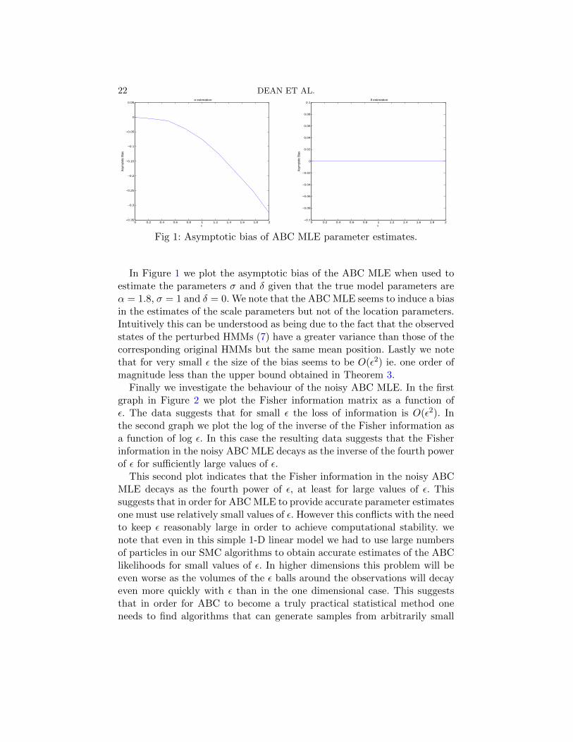
Fig 1: Asymptotic bias of ABC MLE parameter estimates.
In Figure 1 we plot the asymptotic bias of the ABC MLE when used toestimate the parameters σ and δ given that the true model parameters areα = 1.8, σ = 1 and δ = 0. We note that the ABC MLE seems to induce a biasin the estimates of the scale parameters but not of the location parameters.Intuitively this can be understood as being due to the fact that the observedstates of the perturbed HMMs (7) have a greater variance than those of thecorresponding original HMMs but the same mean position. Lastly we notethat for very small ε the size of the bias seems to be O(ε2) ie. one order ofmagnitude less than the upper bound obtained in Theorem 3.
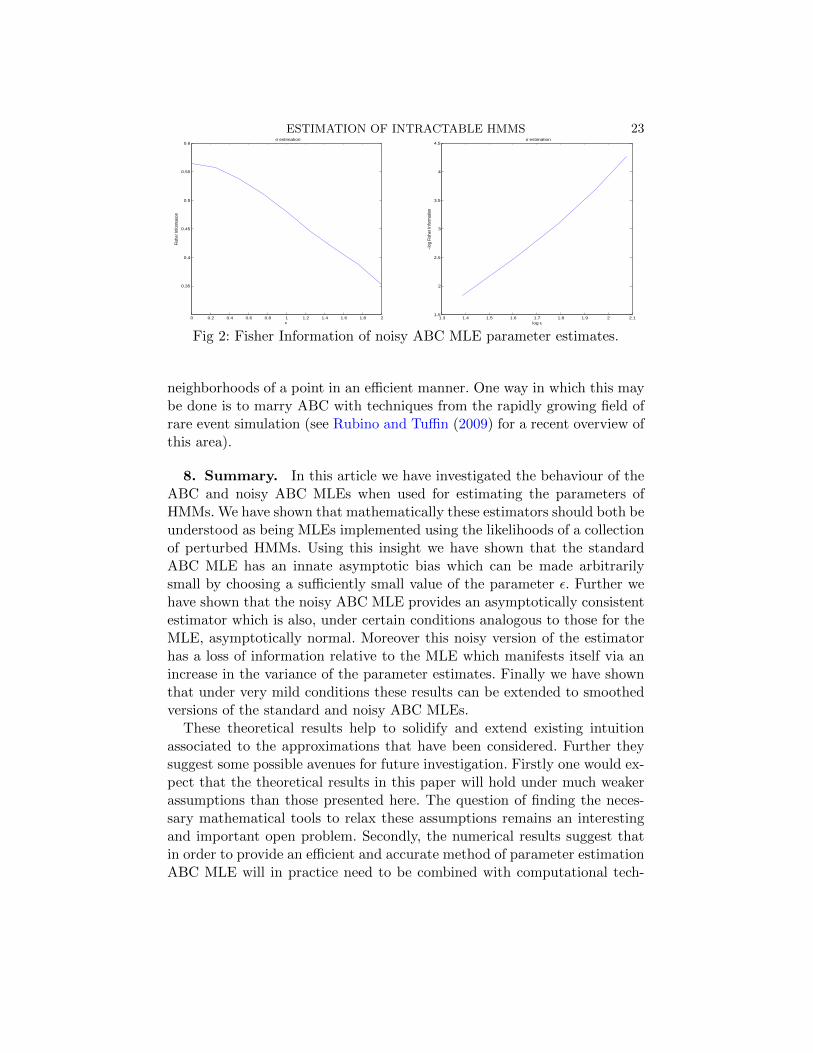
Finally we investigate the behaviour of the noisy ABC MLE. In the firstgraph in Figure 2 we plot the Fisher information matrix as a function ofε. The data suggests that for small ε the loss of information is O(ε2). Inthe second graph we plot the log of the inverse of the Fisher information asa function of log ε. In this case the resulting data suggests that the Fisherinformation in the noisy ABC MLE decays as the inverse of the fourth powerof ε for sufficiently large values of ε.
This second plot indicates that the Fisher information in the noisy ABCMLE decays as the fourth power of ε, at least for large values of ε. Thissuggests that in order for ABC MLE to provide accurate parameter estimatesone must use relatively small values of ε. However this conflicts with the needto keep ε reasonably large in order to achieve computational stability. wenote that even in this simple 1-D linear model we had to use large numbersof particles in our SMC algorithms to obtain accurate estimates of the ABClikelihoods for small values of ε. In higher dimensions this problem will beeven worse as the volumes of the ε balls around the observations will decayeven more quickly with ε than in the one dimensional case. This suggeststhat in order for ABC to become a truly practical statistical method oneneeds to find algorithms that can generate samples from arbitrarily small
ESTIMATION OF INTRACTABLE HMMS 23
0 0.2 0.4 0.6 0.8 1 1.2 1.4 1.6 1.8 2
0.35
0.4
0.45
0.5
0.55
0.6σ estimation
ε
Fish
er In
form
atio
n
1.3 1.4 1.5 1.6 1.7 1.8 1.9 2 2.11.5
2
2.5
3
3.5
4
4.5
log ε
−log
Fis
her I
nfor
mat
ion
σ estimation
Fig 2: Fisher Information of noisy ABC MLE parameter estimates.
neighborhoods of a point in an efficient manner. One way in which this maybe done is to marry ABC with techniques from the rapidly growing field ofrare event simulation (see Rubino and Tuffin (2009) for a recent overview ofthis area).
8. Summary. In this article we have investigated the behaviour of theABC and noisy ABC MLEs when used for estimating the parameters ofHMMs. We have shown that mathematically these estimators should both beunderstood as being MLEs implemented using the likelihoods of a collectionof perturbed HMMs. Using this insight we have shown that the standardABC MLE has an innate asymptotic bias which can be made arbitrarilysmall by choosing a sufficiently small value of the parameter ε. Further wehave shown that the noisy ABC MLE provides an asymptotically consistentestimator which is also, under certain conditions analogous to those for theMLE, asymptotically normal. Moreover this noisy version of the estimatorhas a loss of information relative to the MLE which manifests itself via anincrease in the variance of the parameter estimates. Finally we have shownthat under very mild conditions these results can be extended to smoothedversions of the standard and noisy ABC MLEs.
These theoretical results help to solidify and extend existing intuitionassociated to the approximations that have been considered. Further theysuggest some possible avenues for future investigation. Firstly one would ex-pect that the theoretical results in this paper will hold under much weakerassumptions than those presented here. The question of finding the neces-sary mathematical tools to relax these assumptions remains an interestingand important open problem. Secondly, the numerical results suggest thatin order to provide an efficient and accurate method of parameter estimationABC MLE will in practice need to be combined with computational tech-
24 DEAN ET AL.
niques that allow one to generate samples effectively from sets with verysmall probabilities. The question of finding a generally applicable methodof doing this is the topic of our current research.
Appendix A: Auxiliary Results. Here we present some supportingtechnical lemmas. The first result is a standard result from real analysiswhich we state without proof.
Lemma 5. Suppose that there exists a function f : Ru → Rv and se-quence of continuously differentiable functions fn : Ru → Rv, n ≥ 1, suchthat fn(z),∇θfn(z) are bounded uniformly in n and z, fn(z) → f(z) uni-formly in z and the sequence ∇θfn(z) is Cauchy uniformly in z. Then fis itself uniformly bounded and continuously differentiable and ∇θf(z) =limn→∞∇θfn(z) uniformly in z.
The second lemma is concerned with the identifiability of probability dis-tributions under additive noise.
Lemma 6. Let distributions µ1, µ2 and ν on Rm for some m ≥ 1 begiven and suppose that the characteristic function of ν is equal to zero on aset of Lebesgue measure zero. Then
µ1 = µ2 ⇐⇒ µ1 ∗ ν = µ2 ∗ ν.
Proof. For any distribution µ we shall let ϕµ(λ) denote the correspond-ing characteristic function. It is well known that for any pair of randomvariables µ and ν, ϕµ∗ν(λ) = ϕµ(λ)ϕν(λ) and that µ = ν if and only ifϕµ(λ) = ϕν(λ) for all λ. Thus we have that
µ1 = µ2 ⇐⇒ ϕµ1(λ) = ϕµ2(λ) for all λ
⇐⇒ ϕµ1(λ)ϕν(λ) = ϕµ2(λ)ϕν(λ) for all λ
⇐⇒ µ1 ∗ ν = µ2 ∗ ν.
The following three Lemmas are well known results concerned with theconnectedness of the support of a measure. We state them without proof.
Lemma 7. Let a probability distribution µ on Rm for some m ≥ 1 begiven. Then for all ε > 0 the set
Fµ,ε :={y ∈ Rm : Pµ
(Y ∈ Bε
y
)= 0}
ESTIMATION OF INTRACTABLE HMMS 25
is measurable andPµ (Fµ,ε) = 0.
Lemma 8. If the support of µ is connected then so is the support of then-fold product measure µ⊗n for any n ≥ 1.
Lemma 9. Suppose that the support of a probability measure µ on Rm isconnected (see Section 2.1), then so is the support of the probability measureµ ∗ UBε0 for any ε > 0.
The next lemma shows that adding noise to an observation will, in general,result in a loss of information. The lemma after shows that for very largeamounts of noise the loss in information will be almost complete.
Lemma 10. Suppose that there exists a collection of distributions Pθ onsome Y ⊂ Rm parameterised by θ ∈ Θ and with densities pθ (·) with respectto some common finite dominating measure µ, and that the densities pθ (·)are differentiable w.r.t. θ. For all θ ∈ Θ and ε > 0 let Pεθ = Pθ ∗ UBε0. Thenfor any θ ∈ Θ and ε > 0
(24) EPθ[∇θ log pθ(Y ).∇θ log pθ(Y )T
]≥ EPεθ
[∇θ log pεθ(Y ).∇θ log pεθ(Y )T
]where pεθ(·) denotes the density of the distribution Pεθ with respect to thefinite dominating measure µ ∗ UBε0. Furthermore, if the supports of the dis-tributions Pθ are all connected then we have equality in (24) if and only ifboth quantities are equal to the zero matrix.
Proof. Let θ ∈ Θ be given and let Y be a random variable distributedaccording to pθ(·). Observe that given ε the quantity pεθ(·) is equal to thedensity of the random variable Y ε = Y + εZ (with respect to the appro-priate dominating measure) where Z is an independent random variableand Z ∼ UB1
0. By a straightforward application of the Fisher identity and
the fact that pθ(Y, Yε) = pθ(Y )IBε(Y ε − Y ) one has that ∇θ log pεθ(Y
ε) =E [∇θ log pθ(Y, Y
ε)|Y ε] = E [∇θ log pθ(Y )|Y ε] a.s. where pθ(·, ·) denotes thejoint density of the random variables Y, Y ε from which it follows that forany v ∈ Rm, vT∇θ log pεθ(Y
ε) = E[vT∇θ log pθ(Y )|Y ε
]. Furthermore given
v ∈ Rm we have that(25)
vTEPθ[∇θ log pθ(Y ).∇θ log pθ(Y )T
]v = EPθ
[vT∇θ log pθ(Y ).∇θ log pθ(Y )T v
],
vTEPεθ
[∇θ log pεθ(Y ).∇θ log pεθ(Y )T
]v = EPεθ
[vT∇θ log pεθ(Y ).∇θ log pεθ(Y )T v
].
26 DEAN ET AL.
Applying Jensen’s inequality to (25) yields
vTEPθ[∇θ log pθ(Y ).∇θ log pθ(Y )T
]v ≥ vTEPεθ
[∇θ log pεθ(Y ).∇θ log pεθ(Y )T
]v
for all v ∈ Rm from which (24) immediately follows.We now prove the second assertion. Since the mapping z ∈ R → z2
is strictly convex it further follows from Jensen’s inequality that for anyv ∈ Rm,
vTEPθ[∇θ log pθ(Y ).∇θ log pθ(Y )T
]v = vTEPεθ
[∇θ log pεθ(Y ).∇θ log pεθ(Y )T
]v
if and only if vT∇θ log pθ(Y ) and hence vT∇θ log pθ(Y, Yε) is σ (Y ε) measur-
able. Thus equality holds in (24) if and only if vT∇θ log pθ(Y, Yε) is σ (Y ε)
measurable for all v ∈ Rm which holds if and only if ∇θ log pθ(Y, Yε) is
σ (Y ε) measurable. Hence in order to prove the final part of the resultit is sufficient to show that ∇θ log pθ(Y, Y
ε) is σ (Y ε) measurable if andonly if it is equal to zero a.s. Assume that ∇θ log pθ(Y, Y
ε) is σ (Y ε) mea-surable. Then ∇θ log pθ(Y
ε) = ∇θ log pθ(Y, Yε) a.s.. Using the fact that
∇θ log pθ(y, yε) = ∇θ log pθ(y)IBε(yε − y) one then has that
(26) ∇θ log pθ(y) = ∇θ log pθ(y′)
for Pθ a.s. all y, y′ such that |y − y′| ≤ 2ε.Suppose now that ∇θ log pθ(Y ) is not Pθ a.s. constant. Then there must
exist v and η such that Pθ(|∇θ log pθ(Y ) − v| ≤ η),Pθ(|∇θ log pθ(Y ) − v| >η) > 0. It then follows from Lemma 7 that there must exist points y and ysuch that for all δ > 0
(27)Pθ(|Y − y| ≤ δ, |∇θ log pθ(Y )− v| ≤ η) > 0,
Pθ(|Y − y| ≤ δ, |∇θ log pθ(Y )− v| ≤ η) > 0.
Since the support of Pθ is connected there exists a continuous curve C :[0, 1]→ Rm contained in the support of Pθ such that C(0) = y and C(0) = y.By the continuity of C one can find a finite sequence of open balls Bo
1, . . . , Bon
of radius less than or equal to ε such that y ∈ Bo1, y ∈ Bo
n, C ⊂ ∪nk=1Bok
and such that for every 1 ≤ k < n, Bok ∩ Bo
k+1 ∩ C 6= ∅. Consider any twoneighbouring balls Bo
k and Bok+1. From the above we have that ∇θ log pθ(·) is
Pθ a.s. constant on Bok and Bo
k+1 and that there exists some ball contained inBok∩Bo
k+1 with non zero Pθ mass and thus that∇θ log pθ(·) is Pθ a.s. constanton Bo
k ∪ Bok+1. Hence it follows that ∇θ log pθ(·) is Pθ a.s. constant ∪nk=1B
ok
which contradicts the assumption that ∇θ log pθ(Y ) is not Pθ a.s. constant.Thus it follows that if ∇θ log pθ(Y, Y
ε) is σ (Y ε) measurable that ∇θ log pθ(·)
ESTIMATION OF INTRACTABLE HMMS 27
must be Pθ a.s. equal to some constant K. Further, since E [∇θ log pθ(Y )] = 0it then follows that K = 0. Conversely if ∇θ log pθ(·) = 0 a.s. then clearly itis σ (Y ε) measurable.
Lemma 11. Suppose that there exists a collection of distributions Pθ onsome Y ⊂ Rm parameterised by the parameter vector θ ∈ Θ. Assume thatfor every θ the corresponding distribution has a density pθ (·) with respectto some common finite dominating measure µ, that the densities pθ (·) arecontinuously differentiable w.r.t. θ and that the corresponding score functions∇θ log pθ (·) are uniformly bounded above in norm by some some K < ∞.For all θ and ε let Pεθ = Pθ∗UBε0. Then for any θ and any sequence of positivereal numbers εn such that εn ↗∞
limn→∞
Pεnθ({y :
∣∣∇θ log pεnθ (y)∣∣ > δ}
)= 0
for all δ > 0 where pεnθ (·) denotes the density of the distribution Pεnθ withrespect to the finite dominating measure µ ∗ UBεn0 .
Proof. Let θ ∈ Θ be given and let Y be a random variable distributedaccording to Pθ. As in the proof of Lemma 10 we observe that given ε thequantity pεθ(·) is equal to the density of the random variable Y ε = Y + εZ(again with respect to the appropriate dominating measure) where Z is anindependent random variable with Z ∼ UB1
0. Standard computations show
that for any y
∇θ log pεnθ (y) =∇θ∫pθ(z)IBεn (y − z) ν(dz)∫
pθ(z)IBεn (y − z) ν(dz)
=∇θ∫pθ(z)
(1− I(Bεn )C (y − z)
)ν(dz)∫
pθ(z)IBεn (y − z) ν(dz)
=−∫∇θpθ(z)I(Bεn )C (y − z) ν(dz)∫pθ(z)IBεn (y − z) ν(dz)
where the last equality follows from the dominated convergence theoremby (A2), (A3), (A4) and (A5). Since |∇θ log pθ (y)| ≤ K it follows that∣∣∣∫ ∇θpθ(z)I(Bεn )C (y − z) ν(dz)
∣∣∣ ≤ KPθ(Y n ∈ (Bεn
y )C)
for all y. Hence the
proof will follow once we establish that for any δ′
(28) lim supn→∞
Pεnθ({y : Pθ
(Y ∈ Bεn
y
)≤ 1− δ′}
)≤ δ′.
Note that given any δ′ there exist R <∞ and r < 1 such that Pθ(Y ∈ BR
0
),
P (Z ∈ Br0) > 1 − δ′/2 and thus that for any εn > 2R/ (1− r) we have
28 DEAN ET AL.
that Pθ(Y ∈ BR
0 , Y + εnZ ∈ Bεn−R0
)> 1 − δ′. Clearly if y ∈ Bεn−R
0 then
Pθ(Y ∈ Bεn
y
)≥ Pθ
(Y ∈ BR
0
)> 1− δ′/2 and so the result follows.
The following result establishes a stability-like property of the filter as theamount of noise in certain components of the observations becomes infinite.Before we state the result we recall the extended HMM defined in Section 6.Given a HMM {Xk, Yk}k≥0 and a perturbed version {Xk, Y
εk }k≥0 (see (7))
we define the extended HMM to be the joint process {Xk, Yk, Yεk }k≥0. In
other words given a HMM {Xk, Yk}k≥0 and some ε > 0 the extended HMMis the process
(29) {Xk, Yk, Yεk }k≥0 := {Xk, Yk, Yk + εZk}k≥0
where {Zk}k≥0 is such that for each k ≥ 0, Zki.i.d.∼ UB1
0.
Lemma 12. Let {Xk, Yk}k≥0 be a HMM which satisfies (A3) and let{Xk, Yk, Y
εk }k≥0 be the corresponding extended HMM defined in (29). Then
for any l < m, sequences j1 < · · · < jr, j1 < · · · < js, any j ≤ min{l, j1, j1
},
x ∈ X and δ > 0
limε→∞
P(∥∥∥p(Xl:m|Yj1:jr ;Y
εj1:js
;Xj = x)
−p(Xl:m|Yj1:jr ;Xj = x
)∥∥∥TV
> δ)
= 0.(30)
Proof. Clearly we can assume that {j1, . . . , jr} ∩{j1, . . . , js
}= ∅. Let
k = max{m, jr, js
}, then using assumption (A3) and the well known identity
p(Xl:m|Yj1:jr ;Y
εj1:js
;Xj = x)
=
∫ ∏ku=j+1 q(xu−1, xu)
∏rv=1 g(Yjv |xjv)
∏sw=1 g
ε(Y εjw|xjw)dµ(xj+1:l−1;m+1:k)∫ ∏k
u=j+1 q(xu−1, xu)∏rv=1 g(Yjv |xjv)
∏sw=1 g
ε(Y εjw|xjw)dµ(xj+1:k)
(31)
where gε(·|·) is as in (6) it follows that in order to show (30) it is sufficientto show that for any l and δ > 0
(32) limε→∞
P
(supx,x′∈X
∣∣∣∣ gε(Y εl |x)
gε(Y εl |x′)
− 1
∣∣∣∣ > δ
)= 0.
ESTIMATION OF INTRACTABLE HMMS 29
In order to prove (32) it is sufficient, by assumption (A3), to show that forany δ > 0
(33) limε→∞
ν ∗ UBε0
(y : sup
x,x′∈X
∣∣∣∣∣∫Bεyg(y′|x)ν(dy′)∫
Bεyg(y′|x′)ν(dy′)
− 1
∣∣∣∣∣ > δ
)= 0.
By assumption (A3) we have that for any δ′ > 0 there exists some Rδ′ <∞such that for all x ∈ X ∫
(BRδ′0 )C
g(y|x)ν(dy) < δ′.
It then follows that given the above δ there exists some Rδ < ∞ such that
supx,x′∈X
∣∣∣∣ ∫Bεy g(y′|x)ν(dy′)∫Bεy
g(y′|x′)ν(dy′)− 1
∣∣∣∣ ≤ δ for all y such that BRδ0 ⊂ Bε
y. Thus in
order to prove (33) it is sufficient to show that for any R > 0, limε→∞ ν ∗UBε0
((Bε−R
0 )C)
= 0. However for any r ∈ (0, 1) we have that
lim supε→∞
ν ∗ UBε0(
(Bε−R0 )C
)≤ lim sup
ε→∞ν ∗ UBε0
((B
(1−r)ε0 )C
)≤ lim sup
ε→∞
(ν((Brε
0 )C)
+ UBε0(
(B(1−2r)ε0 )C
))from which the result follows.
The next five results are restatements of certain well-known stability prop-erties of the filter.
Lemma 13. Let {Xk, Yk} be a HMM which satisfies (A3) and let theprocess {Xk, Yk, Y
εk } be the corresponding extended HMM defined as in (29).
Then for all k ≤ l < m ≤ n, j1 < · · · < jr and j1 < · · · < js suchthat j1 ∧ j1 ≥ k, jr ∨ js ≤ n, all xk, x
′k, xn, x
′n ∈ X and all sequences
Yj1 , . . . , Yjr ;Yεj1, . . . , Y ε
js∥∥∥P(Xl:m|Yj1:r ;Y εj1:s
;Xk = xk
)− P
(Xl:m|Yj1:r ;Y ε
j1:s;Xk = x′k
)∥∥∥TV≤ ρ(l−k)
(34)
and∥∥∥P(Xl:m|Yj1:r ;Y εj1:s
;Xk = xk;Xn = xn
)−P(Xl:m|Yj1:r ;Y ε
j1:s;Xk = x′k, Xn = x′n
)∥∥∥TV≤ 2ρ(l−k)∧(n−m)
(35)
where ρ =(1− c2
1
/c2
1
).
30 DEAN ET AL.
Proof. Equations (34) and (36) follow immediately from standard re-sults in the literature, see for example Del Moral (2004) and Cappe, Rydenand Moulines (2005).
Corollary 1. Let {Xk, Yk} be a HMM which satisfies (A3) and letthe process {Xk, Yk, Y
εk } be the corresponding extended HMM defined as in
(29). Then for all l ≤ m and infinite sequences . . . , j−1, j0 and j0, j1, . . . the
conditional probability laws p(Xl:m|Yj−∞:0
)and p
(Xl:m|Yj−∞:0 ;Y ε
j0:∞
)exist
and are well defined. Further for any x ∈ X
(36)∥∥∥P(Xl:m|Yj−k:0 ;Y ε
j0:n;X−k = x
)− P
(Xl:m|Yj−∞:0 ;Y ε
j0:∞
)∥∥∥TV→ 0,
(37)∥∥P (Xl:m|Yj−k:0 ;X−k = x
)− P
(Xl:m|Yj−∞:0
)∥∥TV→ 0
as k, n→∞.
Proof. Equations (36) and (37) are simple consequences of (34).
Corollary 2. Let {Xk, Yk} be a HMM which satisfies (A3) and let{Xk, Yk, Y
εk } be the corresponding extended HMM defined as in (29). Then
for all k < l, j1 < · · · < jr and j1 < · · · < js such that j1 ∧ j1 ≥ k, all x ∈ Xand all sequences Yj1 , . . . , Yjr ;Y
εj1, . . . , Y ε
js
(38)c3
1
c21
≤ p(xl|Yj1:r ;Y εj1:s
;Xk = x) ≤ c31
c21
where the constants c1, c1 are as in (A3) and the central quantity in (38)denotes the density of the corresponding conditional probability with respectto the dominating measure µ.
Proof. To simplify the exposition we shall only give a proof of (38) forconditional probabilities of the form p(xl|Yj1:r), the proof in the general casefollowing in an identical manner.
It is clear by (A3) that when jr < l
(39) c1 ≤ p(xl|Yj1:r ;Xk = x) ≤ c1
Consider the case when jr ≥ l. Let r′ be such that jr′−1 < l ≤ jr′ . By (A3)we have
p(Yjr′:r |Xl = xl) ≤c2
1
c21
p(Yjr′:r |X′l = x′l)
ESTIMATION OF INTRACTABLE HMMS 31
for any x′l . Note that if l < jr′ one obtains the tighter bound p(Yjr′:r |Xl =xl) ≤ (c1/c1)p(Yjr′:r |X
′l = x′l). Thus
p(xl|Yj1:r ;Xk = x) =p(xl|Yj1:r′−1
;Xk = x)p(Yjr′:r |Xl = xl)∫p(x′l|Yj1:r′−1
;Xk = x)p(Yjr′:r |Xl = x′l)µ(dx′l)
≤ p(xl|Yj1:r′−1;Xk = x)
c21
c21
and the upper bound in (38) is obtained using (39). The lower bound in (38)is proved similarly.
Corollary 3. Let {Xk, Yk} be a HMM which satisfies (A3) and and let{Xk, Yk, Y
εk } be the corresponding extended HMM defined as in (29). Then
for all k ≤ l ≤ l′ < m ≤ m′, j1 < · · · < jr and j1 < · · · < js such thatj1 ∧ j1 ≥ k, and all f, h ∈ L∞, x ∈ X∣∣∣E [f(Xl:l′)|Yj1:r ;Y ε
j1:s;Xk = x
].E[h(Xm:m′)|Yj1:r ;Y ε
j1:s;Xk = x
]−E
[f(Xl:l′)h(Xm:m′)|Yj1:r ;Y ε
j1:s;Xk = x
]∣∣∣ ≤ ‖f‖∞ ‖h‖∞ ρm−l′(40)
where ρ is as in Lemma 13.
Proof. Let
∆H = h(Xm:m′)− E[h(Xm:m′)|Yj1:r ;Y ε
j1:s;Xk = x
].
It follows from (34) that∣∣∣E [∆H|Yj1:r ;Y εj1:s
;Xk = x;Xl
]∣∣∣ ≤ ‖h‖∞ ρm−l′ .The proof is completed by noting that the difference of the two expectationsin (40) can be expressed as
E[f(Xl:l′)∆H|Yj1:r ;Y ε
j1:s;Xk = x
].
Remark 7. The proof of Corollary 3 actually yields the stronger resultthat the left hand side of (40) is bounded above by
‖h‖∞ ρm−l′E
[|f(Xl:l′)| |Yj1:r ;Y ε
j1:s;Xk = x
].
32 DEAN ET AL.
Corollary 4. Let {Xk, Yk} be a HMM which satisfies (A3) and and let{Xk, Yk, Y
εk } be the corresponding extended HMM defined as in (29). Then
for all k′ ≤ k ≤ l < m, j1 < · · · < jr and j1 < · · · < js such that j1∧ j1 ≥ k′,f ∈ L∞, x, x′ ∈ X and 1 ≤ rb ≤ re ≤ r, 1 ≤ sb ≤ se ≤ s such thatjrb ∧ jsb ≥ k, jre ∧ jse ≥ m and l ≥ jrb ∨ jsb we have that∣∣∣E [f(Xl:m)|Yj1:r ;Y ε
j1:s;Xk′ = x′
]− E
[f(Xl:m)|Yjrb:re ;Y ε
jsb:se;Xk = x
]∣∣∣≤ 2 ‖f‖∞ ρ
(jre∧jse−m)∧(l−jrb∨jsb )(41)
where ρ is as in Lemma 13.
Proof. It is clear that Yjrb:re ⊆ Yj1:r and Y εjsb:se
⊆ Y εj1:s
. By conditioning
on Xjrb∨jsband Xjre∧jse , the difference of the two expectations in the left
hand-side of (41) can be expressed as∫ ∣∣∣E [f(Xl:m)|Yjrb:re ;Y εjsb:se
;x′jrb∨jsb
;x′jre∧jse
]−E
[f(Xl:m)|Yjrb:re ;Y ε
jsb:se;xjrb∨jsb
;xjre∧jse
]∣∣∣× p
(x′jrb∨jsb
, x′jre∧jse
|Yj1:r ;Y εj1:s
;Xk′ = x′)
× p(xjrb∨jsb
, xjre∧jse |Yjrb:re ;Y εjsb:se
;Xk = x)
× µ(dx′jrb∨jsb
)µ(dx′jre∧jse
)µ(dxjrb∨jsb)µ(dxjre∧jse ).
The result now follows by bounding the difference of the two conditionalexpectations in the integrand using (35).
Remark 8. Using exactly the same proofs as above one can show thatthe conclusions of Corollaries 3 and 4 and Remark 7 are still valid if thefunctions f(Xl:l′), h(Xm:m′) and f(Xl:m) in the statements of those resultsare replaced with the functions f(Xl:l′ , Yl:l′), h(Xm:m′ , Ym:m′), f(Xl:m, Yl:m).
The next result establishes certain properties of the gradient of the filterconditioned on the infinite past, see Le Gland and Mevel (2000) or Tadicand Doucet (2005) for further information concerning the gradient of thefilter.
Lemma 14. Let {Xk, Yk} be a parameterised collection of HMMs whichsatisfy (A3)-(A5) and let {Xk, Yk, Y
εk } be the corresponding extended HMMs
defined as in (29). Then for all θ ∈ G where G is as in assumptions (A4)
ESTIMATION OF INTRACTABLE HMMS 33
and (A5) and every sequence of observations . . . , Y−1;Y ε1 , . . . there exists an
Rd valued function ∇θpθ;Y−∞:−1;Y ε1:∞(x0) in L1(µ) such that such that for all
k, n > 0, x ∈ X
supf :‖f‖∞≤1
∣∣∣∣∫ f(x0)∇θpθ;Y−∞:−1;Y ε1:∞(x0)µ(dx0)
−∫f(x0)∇θpθ (x0|Y−n:−1;Y ε
1:k;X−n = x)µ(dx0)
∣∣∣∣ ≤ Cρn2∧ k2(42)
where ρ is as in Lemma 13, C <∞ is a global constant independent of θ and. . . , Y−1;Y ε
1 , . . . and ∇θpθ (x0|Y−n:−1;Y ε1:k;X−n = x) denotes the gradient of
the density of the conditional law Pθ (x0|Y−n:−1;Y ε1:k;X−n = x) w.r.t. µ.
Furthermore there exists K <∞ such that for all k, n > 0, x and θ ∈ G
(43) ∇θpθ (x0|Y−n:−1;Y ε1:k;X−n = x) , ∇θpθ;Y−∞:−1;Y ε1:∞
(x0) ≤ K
almost surely. Finally we have that for any f ∈ L∞
∇θ∫f(x0)pθ (x0|Y−∞:−1;Y ε
1:∞)µ(dx0)
=
∫f(x0)∇θpθ;Y−∞:−1;Y ε1:∞,...
(x0)µ(dx0),(44)
where (44) defines a continuous function of θ on G.
Proof. We begin by proving (42) and (43). First note that since it issufficient to prove the results component wise with respect to the vectors∇θpθ(·| · · · ) and ∇θpθ(·| · · · ) we can assume that d = 1. For any suitable x,f , n and k∫
f(x0)∇θpθ (dx0|Y−n:−1;Y ε1:k;X−n = x)
=
−1∑j=−n
E [f(X0)∇θ log (qθ(Xj , Xj+1)gθ(Yj |Xj)) |Y−n:−1;Y ε1:k;X−n = x]
(45)
−−1∑
j=−nEθ [f(X0)|Y−n:−1;Y ε
1:k;X−n = x]×
Eθ [∇θ log (qθ(Xj , Xj+1)gθ(Yj |Xj)) |Y−n:−1;Y ε1:k;X−n = x]
(46)
(47)
34 DEAN ET AL.
+k∑l=1
Eθ [f(X0)∇θ log (qθ(Xl−1, Xl)gθ(Yl|Xl)) |Y−n:−1;Y ε1:k;X−n = x]
(48)
−k∑l=1
Eθ [f(X0)|Y−n:−1;Y ε1:k;X−n = x]×
Eθ [∇θ log (qθ(Xl−1, Xl)gθ(Yl|Xl)) |Y−n:−1;Y ε1:k;X−n = x] .
(49)
By (A3), (A5), (41) and Remark 8 we have that for all f : ‖f‖∞ ≤ 1,x, x′ ∈ X , θ ∈ G, k, k′, n, n′ > 0 and j such that −n′ ≤ −n < j < k ≤ k′
that
|E [f(X0)∇θ log (qθ(Xj , Xj+1)gθ(Yj |Xj)) |Y−n:−1;Y ε1:k;X−n = x]
−E[f(X0)∇θ log (qθ(Xj , Xj+1)gθ(Yj |Xj)) |Y−n′:−1;Y ε
1:k′ ;X−n′ = x′]∣∣
≤ 2c1c2
c1
Cρ(j+n)∧(k−j−1)(50)
and
|E [f(X0)|Y−n:−1;Y ε1:k;X−n = x]×
E [∇θ log (qθ(Xj , Xj+1)gθ(Yj |Xj)) |Y−n:−1;Y ε1:k;X−n = x]
− E[f(X0)|Y−n′:−1;Y ε
1:k′ ;X−n′ = x′]×
E[∇θ log (qθ(Xj , Xj+1)gθ(Yj |Xj)) |Y−n′:−1;Y ε
1:k′ ;X−n′ = x′]∣∣ .
≤ 4Cc1c2
c1
(1 + C
c1
c1
)ρ(j+n)∧(k−j−1)(51)
where ρ is as in Lemma 13, C is as in Corollary 4 and c1, c1, c2 are as inassumption (A3) and (A5). Further by (A3), (A5) and (40) it follows thatfor all x ∈ X , θ ∈ G, k, n > 0 and j 6= 0 that
|E [f(X0)∇θ log (qθ(Xj , Xj+1)gθ(Yj |Xj)) |Y−n:−1;Y ε1:k;X−n = x]
− E [f(X0)|Y−n:−1;Y ε1:k;X−n = x]×
E [∇θ log (qθ(Xj , Xj+1)gθ(Yj |Xj)) |Y−n:−1;Y ε1:k;X−n = x]|
≤ 2c1c2
c1
ρ|j|∧|j+1|.(52)
ESTIMATION OF INTRACTABLE HMMS 35
It thus follows from (45)-(52) that for all θ ∈ G that for all k, n ≥ 1
supx,x′∈X
supf :‖f‖∞≤1
∣∣∣∣∫ f(x0)∇θpθ (x0|Y−n:−1;Y ε1:k;X−n = x)µ(dx0)
−∫f(x0)∇θpθ
(x0|Y−n′:−1;Y ε
1:k′ ;X−n′ = x′)µ(dx0)
∣∣∣∣≤ 64C2 c
21c2
c21ρ
∞∑r=n
2∧ k
2
ρr.(53)
Further the first part of (43) follows from (45)-(49), (A3) and (A5), theuniform boundedness of the densities of conditional probability densitiespθ (x0|Y−n:−1;Y ε
1:k;X−n = x) (Corollary 2) and Remark 7. Let K be theconstant bounding the first part of (43) and for any x ∈ X , k, n ≥ 0 andobservations Y−n, . . . , Y−1;Y ε
1 , . . . , Yεk let
∇θpKθ (x0|Y−n:−1;Y ε1:k;X−n = x) = ∇θpθ (x0|Y−n:−1;Y ε
1:k;X−n = x) +K.
(54)
The functions ∇θpKθ (·| · · · ) are densities with respect to µ of a collectionof (random) finite positive measures, each with total mass equal to Kand for which (53) clearly still holds. Since the space of positive finitemeasures equipped with the total variation norm is a Banach space (seee.g. Parthasarathy and Steerneman (1985)) it follows from (53) that givena doubly infinite sequence of observations . . . , Y−1;Y ε
1 , . . . there exists somepositive finite measure µKY−∞:−1;Y ε1:∞
such that for any n ≥ 1
supx∈X
supf :‖f‖∞≤1
∣∣∣∣∫ f(x0)∇θpKθ (x0|Y−n:−1;Y ε1:n;X−n = x)µ(dx0)
−∫f(x0)µKY−∞:−1;Y ε1:∞
(dx0)
∣∣∣∣ ≤ 64C2 c21c2
c21ρ(1− ρ)
ρn2 .(55)
It follows by definition that ∇θpKθ (·| · · · ) ≤ 2K and thus from (55) thatµKY−∞:−1;Y ε1:∞
� µ and that its density ∇θpKθ;Y−∞:−1;Y ε1:∞(·) is bounded above
by 2K. Equation (42) and the second part of equation (43) now follow byletting ∇θpθ;Y−∞:−1;Y ε1:∞
(·) = ∇θpKθ;Y−∞:−1;Y ε1:∞(·) − K. We shall prove (44)
by, for any f ∈ L∞, applying Lemma 5 to the sequence of functions
(56) Eθ [f(X0)|Y−n:−1;Y ε1:n;X−n = x]
for n ≥ 1 and x ∈ X arbitrary. Clearly the sequence of functions in (56) arecontinuously differentiable by (A2) and (A4). In order to be able to apply
36 DEAN ET AL.
Lemma 5 we further need to establish that the functions in (56) and theirderivatives are uniformly bounded. This follows from (38) and (43), that
Eθ [f(X0)|Y−n:−1;Y ε1:n;X−n = x]→ Eθ [f(X0)|Y−∞:−1;Y ε
1:∞]
uniformly which follows from (36) and finally that the sequence of derivativesof the functions in (56) is uniformly Cauchy which follows from (42).
Corollary 5. Assume the same conditions as in Lemma 14. Thenresults analogous to those in (42), (43) and (44) hold for the gradients ofthe conditional densities pθ (x0|Y−n:−1;X−n = x), pεθ
(x0|Y ε
−n:−1;X−n = x)
and pθ (x0|Y−∞:−1;Y εm:∞). Furthermore for every sequence of observations
Y−∞:−1, Y ε1:∞ and integer m ≥ 1
(57) |∇θpθ (x0|Y−∞:−1;Y εm:∞)−∇θpθ (x0|Y−∞:−1)| ≤ Cρ
m2
where ρ is as in Lemma 13 and C <∞ is a global constant independent ofθ, x0, Y−∞:−1, Y ε
1:∞ and m.
Proof. The first part of the corollary can be proved in exactly the sameway as Lemma 14.
To prove the second part of the corollary it is sufficient to show that(58)|∇θpθ (x0|Y−n:−1;Y ε
m:n;X−n = x)−∇θpθ (x0|Y−n:−1;X−n = x)| ≤ Cρm2∧n
2
for some C and all θ, Y−∞:−1, Y ε1:∞, x and n. Inequality (58) can be es-
tablished by decomposing the two gradients that appear on its left handside in an analogous manner to (45)-(49). The bound on the right hand sidethen follows by bounding the terms in this decomposition individually using(50)-(52) and the fact that
(59) Pθ (x0|Y−n:−1;Y εm:n;X−n = x)− Pθ (x0|Y−n:−1;X−n = x) ≤ 2ρm
for all θ, Y−∞:−1, Y ε1:∞, x and n which follows immediately from (35).
Appendix B: Proofs of Lemmas 1, 2, 3 and 4.
Proof of Lemma 1. We begin by observing that a straightforward con-sequence of assumption (A3) is that for all (θ, ε) ∈ Θ × [0,∞), r > 0 andsequences y−r, . . . , y1
(60) c1 ≤ pεθ(y1|y−r . . . , y0) ≤ c1.
ESTIMATION OF INTRACTABLE HMMS 37
Further by Lemma 13 it follows that the finite history conditional likeli-hoods pεθ(y1|y−r, . . . , y0) converge to the infinite history conditional likeli-hoods pεθ(y1| . . . , y0) as r →∞ uniformly in θ, ε, the sequence of observations. . . , y0, y1 and initial distribution π(x−r−1). Thus by (60) it follows that inorder to show continuity w.r.t. the first term and right continuity w.r.t. thesecond term of the mapping (θ, ε) ∈ Θ × [0,∞) → lε(θ) it is sufficient toshow that these properties hold for the mapping
(61) (θ, ε) ∈ Θ× [0,∞)→ Eθ∗ [log pεθ(Y1|Y−r:0)]
for all r > 0. For the rest of the proof we shall assume an arbitrary fixedr > 0 and initial distribution π(x−r−1) are given. Observe that by (A2), (A3)Lemma 7 and the dominated convergence theorem the mapping (θ, ε) ∈ Θ×(0,∞)→ gεθ(y|x) is continuous w.r.t. its first term and right continuous w.r.t.its second term for all y ∈ Y and x ∈ X . Thus by a second application of(A2), (A3) and the dominated convergence theorem one immediately obtainsthese properties of the mapping (θ, ε) ∈ Θ× (0,∞) → pεθ(y1|y−r . . . , y0) forany r > 0 and sequence y−r, . . . , y1. A final application of (A2), (A3) andthe dominated convergence theorem along with the inequality (60) yield thatthe mapping Θ × [0,∞) → R given in (61) is also respectively continuousand right continuous. In order to prove continuity w.r.t. the first term andright continuity w.r.t. the second term of (61) on Θ× [0,∞) we shall showfor any sequences εn ↘ 0 and θn ∈ Θ→ θ ∈ Θ, that
(62) Eθ∗[log pεnθn(Y1|Y−r:0)
]→ Eθ∗ [log pθ(Y1|Y−r:0)]
as n→∞. First note that
Eθ∗[log pεnθn(Y1|Y−r:0)
]= Eθ∗
[log pεnθn(Y−r, . . . , Y1)− log pεnθn(Y−r, . . . , Y0)
].
Thus in order to prove (62) it is sufficient to show that
(63) Eθ∗[log pεnθn(Y−r, . . . , Y1)
]→ Eθ∗ [log pθ(Y−r, . . . , Y1)]
and
(64) Eθ∗[log pεnθn(Y−r, . . . , Y0)
]→ Eθ∗ [log pθ(Y−r, . . . , Y0)]
as n → ∞. We will now conclude the proof of the theorem by proving(63) and observing that the proof of (64) follows in a completely identicalmanner. The differences in the values of the likelihoods in (63) evaluated at
38 DEAN ET AL.
different parameter values θn and θ can be bounded by∣∣pεnθn(Y−r, . . . , Y1)− pεnθ (Y−r, . . . , Y1)∣∣
≤∣∣∣∣ ∫X r+3
[ 1∏k=−r
qθn(xk−1, xk)gεnθn
(Yk|xk)]π(dx−r−1)µ(dx−r:1)
−∫X r+3
[ 1∏k=−r
qθ(xk−1, xk)gεnθn
(Yk|xk)]π(dx−r−1)µ(dx−r:1)
∣∣∣∣+
∣∣∣∣ ∫X r+3
[ 1∏k=−r
qθ(xk−1, xk)gεnθn
(Yk|xk)]π(dx−r−1)µ(dx−r:1)
−∫X r+3
[ 1∏k=−r
qθ(xk−1, xk)gεnθ (Yk|xk)
]πθ(dx−r−1)µ(dx−r:1)
∣∣∣∣≤ cr+2
1
∫X r+3
∣∣∣∣∣1∏
k=−rqθn(xk−1, xk)−
1∏k=−r
qθ(xk−1, xk)
∣∣∣∣∣π(dx−r−1)µ(dx−r:1)
(65)
+ cr+11
(1∑
l=−r
∫X r+3
∣∣gεnθn(Yl|xl)− gεnθ (Yl|xl)∣∣π(dx−r−1)µ(dx−r:1)
)(66)
where c1 is as in (A3) and (66) follows from (A3), the definition of gεθ(·|·)and the telescopic identity
n∏k=1
akbk −n∏k=1
ak bk =n∑l=1
(n∏k=1
ak × (bl − bl)l−1∏k=1
bk
n∏k=l+1
bk
)
which holds for any collection of reals a1, . . . , an; b1, . . . , bn; b1, . . . , bn. Clearlyassumptions (A2) and (A3) and the dominated convergence theorem implythat the quantity in (65) converges to zero as θn converges to θ. Furthermorethe definition of gεθ(·|·) and convergence of θn to θ imply that for any δ > 0the limit supremum of (66) as n→∞ is bounded above by
lim supn→∞
cr+11
1∑l=−r
∫X r+3
∫BεnYl
∆gδθ(y|xl)ν(dy)
ν(BεnYl
)π(dx−r−1)µ(dx−r:1)
(67)
ESTIMATION OF INTRACTABLE HMMS 39
where for all x ∈ X and y ∈ Y
∆gδθ(y|x) = supθ′:|θ′−θ|≤δ
|gθ′(y|x)− gθ(y|x)| .
It then follows from (A3), (67), the dominated convergence theorem andthe Lebesgue differentiation theorem (see Wheeden and Zygmund (1977),Chapter 10) that
lim supn→∞
cr+11
(1∑
l=−r
∫X r+3
∣∣gεnθn(Yl|xl)− gεnθ (Yl|xl)∣∣π(dx−r−1)µ(dx−r:1)
)
≤ cr+11
(1∑
l=−r
∫X r+3
∆gδθ(Yl|xl)π(dx−r−1)µ(dx−r:1)
)(68)
for any δ > 0. Next we observe that by (A2) we have that limδ→0 ∆gδθ(y|x) =0 for all y ∈ Y and x ∈ X and hence that by applying (A3) and the domi-nated convergence theorem to (68) we have that
lim supn→∞
cr+11
(1∑
l=−r
∫X r+3
∣∣gεnθn(Yl|xl)− gεnθ (Yl|xl)∣∣π(dx−r−1)µ(dx−r:1)
)= 0.
(69)
Thus it follows from (60), (65), (66) and (69) that for almost all sequencesof observations Y−r, . . . , Y1 that
limn→∞
log pεnθn(Y−r, . . . , Y1) = limn→∞
log pεnθ (Y−r, . . . , Y1).(70)
Since
pεθ(Y−r, . . . , Y1)
=
∫X r+3
[ 1∏k=−r
qθ(xk−1, xk)
∫BεYk
gθ(y|xk)ν(dy)
ν(BεYk
)
]π(dx−r−1)µ(dx−r:1)
we have that (63) now follows from (60), (70), the Lebesgue differentiationtheorem, (A3) and the dominated convergence theorem.
Proof of Lemma 2. We start by showing that l(θ) is continuously dif-ferentiable. First observe that by (A3), (A4), (A5), (36), (38), (42), (43), (44)
40 DEAN ET AL.
and the dominated convergence theorem we have that for arbitrary x ∈ X
(71)limn→∞
log pθ(Y1|Y−n:0;X−n = x) = log pθ(Y1|Y−∞:0)
limn→∞
∇θ log pθ(Y1|Y−n:0;X−n = x) = ∇θ log pθ(Y1|Y−∞:0)
uniformly in θ ∈ G and . . . , Y0, Y1 and that the quantities in (71) are uni-formly bounded. It follows from (71) that
l(θ) = limn→∞
Eθ∗ [log pθ(Y1|Y−n:0;X−n = x)]
and hence from (71) and Lemma 5 that ∇θl(θ) exists, is continuous and isequal to limn→∞ Eθ∗ [∇θ log pθ(Y1|Y−n:0;X−n = x)]. Since gεθ(y|x) defined in(6) satisfies all the conditions laid out in (A3)-(A5), the same conclusionapplies to lε(θ). To prove the corresponding results for ∇2
θl(θ) observe thatby the Fisher information identity
∇2θEθ∗ [log pθ(Y1|Y−n:0;X−n = x)]
= Eθ∗[∇θ log pθ(Y1|Y−n:0;X−n = x)∇θ log pθ(Y1|Y−n:0;X−n = x)T
].
Existence and continuity of ∇2θl(θ) then follows from (71) and Lemma 5
applied to the functions ∇θ log pθ(Y1|Y−n:0;X−n = x). Furthermore the factthat ∇2
θl(θ∗) = I(θ∗) now follows from Douc, Moulines and Ryden (2004).
We begin the proof of (12) by observing that from (71) and the identitylog pθ(Y1, . . . , Yn|X1 = x) =
∑nk=1 log pθ(Yk|Y1:k−1;X1 = x) we have that
∇θl(θ) = limn→∞
1
nEθ∗ [∇θ log pθ(Y1, . . . , Yn|X1 = x)]
and similarly, for any ε > 0 that
∇θlε(θ) = limn→∞
1
nEθ∗ [∇θ log pεθ(Y1, . . . , Yn|X1 = x)] .
Thus it is sufficient to show that there exists some positive constant R suchthat for any sequence Y1, . . . , Yn, initial distribution π0 and θ ∈ G,
(72) |∇θ log pθ(Y1, . . . , Yn|X1 = x)−∇θ log pεθ(Y1, . . . , Yn|X1 = x)| ≤ nRε.
For all θ ∈ G, sequences Y1, . . . , Yn and Y ε1 , . . . , Y
εn drawn from the original
ESTIMATION OF INTRACTABLE HMMS 41
and perturbed processes respectively and x ∈ X
∇θ log pθ (Y1, . . . , Yn|X1 = x)−∇θ log pεθ (Y ε1 , . . . , Y
εn |X1 = x)
=
n∑i=1
(∇θ log pθ
(Y1:i;Y
εi+1:n|X1 = x
)−∇θ log pθ (Y1:i−1;Y ε
i:n|X1 = x))
=
n∑i=1
(∇θ log pθ
(Yi|Y1:i−1;Y ε
i+1:n;X1 = x)
−∇θ log pθ(Y εi |Y1:i−1;Y ε
i+1:n;X1 = x))
=n∑i=1
(∫∇θgθ (Yi|xi) pθ
(xi|Y1:i−1;Y ε
i+1:n;X1 = x)µ(dxi)
+
∫gθ (Yi|xi)∇θpθ
(xi|Y1:i−1;Y ε
i+1:n;X1 = x)µ(dxi)
)×(∫
gθ (Yi|xi) pθ(xi|Y1:i−1;Y ε
i+1:n;X1 = x)µ(dxi)
)−1
−n∑i=1
(∫∇θgεθ (Y ε
i |xi) pθ(xi|Y1:i−1;Y ε
i+1:n;X1 = x)µ(dxi)
+
∫gεθ (Y ε
i |xi)∇θpθ(xi|Y1:i−1;Y ε
i+1:n;X1 = x)µ(dxi)
)
×(∫
gεθ (Y εi |xi) pθ (xi|Y1:i−1;Yi+1:ε;X1 = x)µ(dxi)
)−1
.
(73)
In particular (73) holds true when Y ε1 , . . . , Y
εn = Y1, . . . , Yn and so (72)
follows from (A3), (A5), (A6), (A7) and (43).
Proof of Lemma 3. Throughout this proof we shall assume that thedensity of any finite collection of random variables from . . . , Y0, Y1, . . . and. . . , Y ε
0 , Yε
1 , . . . is computed assuming that the initial condition of the hiddenstate process has the stationarity distribution Pθ∗ . We begin by observingthat from Douc, Moulines and Ryden (2004) we have that(74)
I(θ∗) = limn→∞
1
nEθ∗
[∇θ log pθ∗ (Y1, . . . , Yn) .∇θ log pθ∗ (Y1, . . . , Yn)T
],
Iε(θ∗) = limn→∞
1
nEθ∗
[∇θ log pεθ∗ (Y ε
1 , . . . , Yεn) .∇θ log pεθ∗ (Y ε
1 , . . . , Yεn)T].
By the Fisher identity we have that for any 1 ≤ k < k′ and subsequences
42 DEAN ET AL.
{j1, . . . , jl} ⊂ {1, . . . , k} and{j′1, . . . , j
′l′}⊂ {k + 1, . . . , k′} that
(75) ∇θ log pθ
(Yj1:l ;Y
εj′1:l′
)= E
[∇θ log pθ
(Y1:k;Y
εk+1:k′
)|Yj1:l ;Y
εj′1:l′
].
Further by construction of the perturbed process one can easily show thatgiven any n and any subset {j1, . . . , jl} ⊂ {1, . . . , n} that
(76) ∇θ log pθ (Y1, . . . , Yn) = ∇θ log pθ(Y1, . . . , Yn;Y ε
j1 , . . . , Yεjl
).
Using (75) and (76) it follows that for any 1 ≤ i < n
Eθ∗[∇θ log pθ∗
(Y1:i, Y
εi+1:n
).∇θ log pθ∗ (Y1:i−1, Y
εi:n)T
]= Eθ∗
[∇θ log pθ∗ (Y1:i−1, Y
εi:n) .∇θ log pθ∗ (Y1:i−1, Y
εi:n)T
],
and hence that
Eθ∗[(∇θ log pθ∗
(Y1:i, Y
εi+1:n
)−∇θ log pθ∗ (Y1:i−1, Y
εi:n))
·(∇θ log pθ∗
(Y1:i, Y
εi+1:n
)−∇θ log pθ∗ (Y1:i−1, Y
εi:n))T ]
= Eθ∗[∇θ log pθ∗
(Y1:i, Y
εi+1:n
).∇θ log pθ∗
(Y1:i, Y
εi+1:n
)T ]− Eθ∗
[∇θ log pεθ∗ (Y1:i−1, Y
εi:n) .∇θ log pεθ∗ (Y1:i−1, Y
εi:n)T
].(77)
Using (77) and (74) and stationarity we have that
I(θ∗)− Iε(θ∗)
= limn→∞
1
n
n∑i=1
Eθ∗[(∇θ log pθ∗
(Y0|Y1−i:−1;Y ε
1:n−i)
−∇θ log pθ∗(Y ε
0 |Y1−i:−1;Y ε1:n−i
))·(∇θ log pθ∗
(Y0|Y1−i:−1;Y ε
1:n−i)
−∇θ log pθ∗(Y ε
0 |Y1−i:−1;Y ε1:n−i
))T]
= limn→∞
Eθ∗[(∇θ log pθ∗ (Y0|Y−n:−1;Y ε
1:n)−∇θ log pθ∗ (Y ε0 |Y−n:−1;Y ε
1:n)
)·(∇θ log pθ∗ (Y0|Y−n:−1;Y ε
1:n)−∇θ log pθ∗ (Y ε0 |Y−n:−1;Y ε
1:n)
)T].
(78)
ESTIMATION OF INTRACTABLE HMMS 43
where the last equality follows from assumptions (A3) and (A5) and equa-tions (34), (43) and (53). In addition, using (42) and the dominated conver-gence theorem, we conclude from (78) that
I(θ∗)− Iε(θ∗) = Eθ∗[(Gθ∗;Y−∞:−1;Y ε1:∞
(Y0)−Gεθ∗;Y−∞:−1;Y ε1:∞(Y ε
0 ))·
(Gθ∗;Y−∞:−1;Y ε1:∞
(Y0)−Gεθ∗;Y−∞:−1;Y ε1:∞(Y ε
0 ))T](79)
where for any sequence . . . , Y−1;Y ε1 , . . .
Gθ∗;Y−∞:−1;Y ε1:∞(Y0) = lim
n→∞∇θ log pθ∗ (Y0|Y−n:−1;Y ε
1:n)
=
(∫ (∇θgθ∗ (Y0|x0) pθ∗ (x0|Y−∞:−1;Y ε
1:∞)
+gθ∗ (Y0|x0) ∇θpθ∗ (x0|Y−∞:−1;Y ε1:∞)
)µ(dx0)
)
×(∫
gθ∗ (Y0|x0) pθ∗ (x0|Y−∞:−1;Y ε1:∞)µ(dx0)
)−1
(80)
and
Gεθ∗;Y−∞:−1;Y ε1:∞(Y ε
0 ) = limn→∞
∇θ log pθ∗ (Y ε0 |Y−n:−1;Y ε
1:n)
=
(∫ (∇θgεθ∗ (Y ε
0 |x0) pθ∗ (x0|Y−∞:−1;Y ε1:∞)
+gεθ∗ (Y ε0 |x0) ∇θpθ∗ (x0|Y−∞:−1;Y ε
1:∞)
)µ(dx0)
)
×(∫
gεθ∗ (Y ε0 |x0) pθ∗ (x0|Y−∞:−1;Y ε
1:∞)µ(dx0)
)−1
.
(81)
Further by using assumptions (A3), (A5) and (34), (42), (43) and (44) wehave that the conditional likelihood functions log pθ∗ (Y0|Y−n:−1;Y ε
1:n) andlog pθ∗ (Y ε
0 |Y−n:−1;Y ε1:n) as well as their derivatives are bounded uniformly
in θ and . . . , Y−1;Y ε1 , . . . and that the derivatives are uniformly Cauchy in
n whilst the conditional likelihoods themselves converge uniformly to thequantities log pθ∗ (Y0|Y−∞:−1;Y ε
1:∞) and log pθ∗ (Y ε0 |Y−∞:−1;Y ε
1:∞). Hence wecan apply Lemma 5 to obtain
(82)Gθ∗;Y−∞:−1;Y ε1:∞
(Y0) = ∇θ log pθ∗(Y0|Y−∞:−1;Y ε1:∞),
Gεθ∗;Y−∞:−1;Y ε1:∞(Y ε
0 ) = ∇θ log pθ∗(Yε
0 |Y−∞:−1;Y ε1:∞).
44 DEAN ET AL.
It now follows from (79) and (82) that
I(θ∗)− Iε(θ∗)
= Eθ∗[(∇θ log pθ∗(Y0|Y−∞:−1;Y ε
1:∞)−∇θ log pθ∗(Yε
0 |Y−∞:−1;Y ε1:∞)
)·(
∇θ log pθ∗(Y0|Y−∞:−1;Y ε1:∞)−∇θ log pθ∗(Y
ε0 |Y−∞:−1;Y ε
1:∞))T]
= Eθ∗[Eθ∗[(∇θ log pθ∗(Y0|Y−∞:−1;Y ε
1:∞)−∇θ log pθ∗(Yε
0 |Y−∞:−1;Y ε1:∞)
)·(
∇θ log pθ∗(Y0|Y−∞:−1;Y ε1:∞)−∇θ log pθ∗(Y
ε0 |Y−∞:−1;Y ε
1:∞))T|Y−∞:−1;Y ε
1:∞
]].
(83)
Finally by applying the Fisher inequality (75) and (76) to the conditionallaws Pθ∗(Y0|Y−∞:−1;Y ε
1:∞) and Pθ∗(Y ε0 |Y−∞:−1;Y ε
1:∞) we get that
Eθ∗[(∇θ log pθ∗(Y0|Y−∞:−1;Y ε
1:∞)−∇θ log pθ∗(Yε
0 |Y−∞:−1;Y ε1:∞)
)·(
∇θ log pθ∗(Y0|Y−∞:−1;Y ε1:∞)−∇θ log pθ∗(Y
ε0 |Y−∞:−1;Y ε
1:∞))T|Y−∞:−1;Y ε
1:∞
]= Eθ∗
[∇θ log pθ∗(Y0|Y−∞:−1;Y ε
1:∞)·
∇θ log pθ∗(Y0|Y−∞:−1;Y ε1:∞)T |Y−∞:−1;Y ε
1:∞
]− Eθ∗
[∇θ log pθ∗(Y
ε0 |Y−∞:−1;Y ε
1:∞)·
∇θ log pθ∗(Yε
0 |Y−∞:−1;Y ε1:∞)T |Y−∞:−1;Y ε
1:∞
]:= I
Y0:Y ε0Y−∞:−1;Y ε1:∞
(θ∗).
(84)
The result now follows from (83) and (84).
Remark 9. Assume (A1)-(A5). Then in exactly the same way as oneproves Lemma 3 one may prove that
I(θ∗) = Iε(θ∗) + Eθ∗[IY0:m−1:Y ε0:m−1
Y−∞:−1;Y εm:∞(θ∗)
]
ESTIMATION OF INTRACTABLE HMMS 45
where for any pair of sequences Y−∞:−1 and Y ε1:∞ and any integer m ≥ 1
IY0:m−1:Y ε0:m−1
Y−∞:−1;Y εm:∞(θ∗)
=1
mEθ∗[∇θ log pθ∗(Y0:m−1|Y−∞:−1;Y ε
m:∞)·
∇θ log pθ∗(Y0:m−1|Y−∞:−1;Y εm:∞)T |Y−∞:−1;Y ε
m:∞
]− 1
mEθ∗[∇θ log pθ∗(Y
ε0:m−1|Y−∞:−1;Y ε
m:∞)·
∇θ log pθ∗(Yε
0:m−1|Y−∞:−1;Y εm:∞)T |Y−∞:−1;Y ε
m:∞
].
(85)
Proof of Lemma 4. We begin by establishing part 1. From (24) and
(84) we have for any Y−∞:−1 and Y ε1:∞ that I
Y0:Y ε0Y−∞:−1;Y ε1:∞
(θ∗) ≥ 0 from which
the first assertion of part 1 immediately follows. In order to prove the secondassertion of part 1 we note that it is sufficient to prove that under the
assumption of connectivity we must have that Eθ∗[IY0:Y ε0Y−∞:−1;Y ε1:∞
(θ∗)]
= 0
implies I(θ∗) = 0. Since we have by Remark 9 that Eθ∗[IY0:Y ε0Y−∞:−1;Y ε1:∞
(θ∗)]
=
Eθ∗[IY0:m−1:Y ε0:m−1
Y−∞:−1;Y εm:∞(θ∗)
]for all m ≥ 1 this will follow once we show that
Eθ∗[IY0:m−1:Y ε0:m−1
Y−∞:−1;Y εm:∞(θ∗)
]= 0 for all m ≥ 1 implies I(θ∗) = 0.
Observe that by Lemmas 8 and 9 and the assumption that ν is connectedit follows that
(ν ∗ UBε0
)⊗mis connected for all ε > 0 and m ≥ 1 and thus
from (A3) and (6) that the conditional laws Pθ∗(Y0:m−1|Y−∞:−1;Y εm:∞) and
Pθ∗(Y ε0:m−1| Y−∞:−1;Y ε
m:∞) are also connected for all ε > 0 and sequencesY−∞:−1 and Y ε
m:∞. It then follows from (24) and (85) that for all m ≥ 1 that
Eθ∗[IY0:m−1:Y ε0:m−1
Y−∞:−1;Y εm:∞(θ∗)
]= 0 implies that
Eθ∗[∇θ log pθ∗(Y0:m−1|Y−∞:−1;Y ε
m:∞)·
∇θ log pθ∗(Y0:m−1|Y−∞:−1;Y εm:∞)T |Y−∞:−1;Y ε
m:∞
]= Eθ∗
[∇θ log pθ∗(Y
ε0:m−1|Y−∞:−1;Y ε
m:∞)·
∇θ log pθ∗(Yε
0:m−1|Y−∞:−1;Y εm:∞)T |Y−∞:−1;Y ε
m:∞
]
46 DEAN ET AL.
for all Y−∞:−1,Y εm:∞ a.s. and hence by Lemma 10 that
∇θ log pθ∗(Y0:m−1|Y−∞:−1;Y εm:∞) = 0
pθ∗(Y0:m−1|Y−∞:−1;Y εm:∞) a.s. and thus by Fisher’s identity applied to the
conditional probabilities that
(86) ∇θ log pθ∗(Y0|Y−∞:−1;Y εm:∞) = 0
pθ∗(Y0|Y−∞:−1;Y εm:∞) a.s. also. Finally observe that one can derive expres-
sions for the gradients of the conditional densities pθ∗(Y0|Y−∞:−1;Y εm:∞) and
pθ∗(Y0|Y−∞:−1) analogous to (80) and (82). It then follows from these and(A3), (A5), (35), (36), (37) and (57) that
(87) ∇θ log pθ∗(Y0|Y−∞:−1) = limm→∞
∇θ log pθ∗(Y0|Y−∞:−1;Y εm:∞)
a.s.. It now follows from (86) and (87) that if Eθ∗[IY0:m−1:Y ε0:m−1
Y−∞:−1;Y εm:∞(θ∗)
]= 0
for all m ≥ 1 then ∇θ log pθ∗(Y0|Y−∞:−1) = 0 a.s. and hence that I(θ∗) = 0.Next we establish part 2. Recall that given a positive semi-definite matrix
M ∈ Rd×d and a sequence of Rd×d valued positive semi-definite matrices{Mn}n≥1 that Mn → M if and only if vTMnv → vTMv for all v ∈ Rd.Thus in order to prove part 2 it is sufficient to show that for every sequence
εn ↗∞ and every v ∈ Rm that vT Eθ∗[IY0:Y ε0Y−∞:−1;Y ε1:∞
(θ∗)]v → vT I (θ∗) v. By
definition and stationarity
vT Eθ∗[IY0:Y ε0Y−∞:−1;Y ε1:∞
(θ∗)]v
= E[(vT . (∇θ log pθ∗ (Y0|Y−∞:−1;Y ε
1:∞)−∇θ log pθ∗ (Y ε0 |Y−∞:−1;Y ε
1:∞)))2]
(88)
and
(89) vT Iv = E[(vT .∇θ log pθ∗ (Y0|Y−∞:−1)
)2].
Further by assumptions (A3) and (A5) and (43) we have that there existssome K <∞ such that
(90)vT .∇θ log pθ∗ (Y0|Y−∞:−1) , vT .∇θ log pθ∗ (Y0|Y−∞:−1;Y ε
1:∞) ,
vT .∇θ log pθ∗ (Y ε0 |Y−∞:−1;Y ε
1:∞) ≤ K
a.s. for all ε > 0 and sequences . . . , Y−1;Y ε1 , . . .. The proof of the second part
of the result will follow from (88), (89) and (90) once we show that for any
ESTIMATION OF INTRACTABLE HMMS 47
. . . , Y−1;Y ε1 , . . .
(91)∇θ log pθ∗ (Y ε
0 |Y−∞:−1;Y ε1:∞)→ 0,
∇θ log pθ∗ (Y0|Y−∞:−1;Y ε1:∞)→ ∇θ log pθ∗ (Y0|Y−∞:−1)
as ε → ∞ in pθ∗ (Y0|Y−∞:−1;Y ε1:∞) probability. The first part of (91) is a
straightforward consequence of applying Lemma 11 to the conditional lawsPθ∗ (Y0|Y−∞:−1;Y ε
1:∞). To establish the second part of (91) observe that from(34), (42), (44), (82) and (80) we have that there exists some C < ∞ suchthat for all . . . , Y−1;Y ε
1 , . . .
(92)|∇θ log pθ∗ (y|Y−∞:−1;Y ε
1:∞)−∇θ log pθ∗ (y|Y−n:−1;Y ε1:n)| ≤ Cρn/2
|∇θ log pθ∗ (y|Y−∞:−1)−∇θ log pθ∗ (y|Y−n:−1)| ≤ Cρn/2
for all n ≥ 1, ε > 0 and y ∈ Y. It then follows from (A3), (A5) and (43),the representation of the score functions ∇θ log pθ∗ (·| · · · ) given in (73), therepresentation of integrals w.r.t. the filter gradients given in (45)-(49) andLemma 12 that
(93) ∇θ log pθ∗ (Y0|Y−n:−1;Y ε1:k)→ ∇θ log pθ∗ (Y0|Y−n:−1)
in probability as ε↗∞. One can then conclude that the second part of (91)holds via (92) and (93). In order to complete the proof of the lemma recall thetwo random variables Gθ∗;Y−∞:−1;Y ε1:∞
(Y0) and Gεθ∗;Y−∞:−1;Y ε1:∞(Y ε
0 ) defined in
(80) and (81). It follows from (A3), (A5) and the Lebesgue differentiationtheorem that Gθ∗;Y−∞:−1;Y ε1:∞
(Y0)→ Gεθ∗;Y−∞:−1;Y ε1:∞(Y ε
0 ) a.s. as ε↘ 0. Since
it follows from the proof of (82) that there exists some K < ∞ such thatfor all ε > 0 the functions Gθ∗;Y−∞:−1;Y ε1:∞
(Y0) and Gεθ∗;Y−∞:−1;Y ε1:∞(Y ε
0 ) arebounded above by K for all . . . , Y−1, Y0;Y ε
1 , . . . we have that part 3 followsfrom (84) and a simple application of the dominated convergence theorem.Finally, part 4 is a trivial consequence of (79), (80) and (81) and assumptions(A3), (A6) and (A7).
References.
Andrieu, C., Doucet, A. and Tadic, V. (2009). On-line Parameter Estimation in Gen-eral State Space Models Using Pseudo Likelihood Technical report, Department ofStatistics, University of Bristol.
Beaumont, M., Zhang, W. and Balding, D. (2002). Approximate Bayesian Computa-tion in Population Genetics. Genetics 162 2025–2035.
Campillo, F. and Rossi, V. (2009). Convolution Particle Filter for Parameter Estimationin General State-Space Models. IEEE Trans. Aero. Elec. Sys. 45 1073–1072.
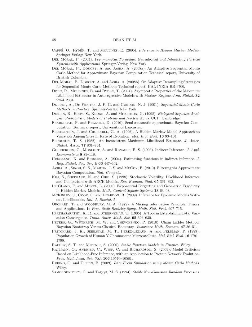
48 DEAN ET AL.
Cappe, O., Ryden, T. and Moulines, E. (2005). Inference in Hidden Markov Models.Springer-Verlag: New York.
Del Moral, P. (2004). Feynman-Kac Formulae: Genealogical and Interacting ParticleSystems with Applications. Springer-Verlag: New York.
Del Moral, P., Doucet, A. and Jasra, A. (2008a). An Adaptive Sequential MonteCarlo Method for Approximate Bayesian Computation Technical report, University ofBristish Columbia.
Del Moral, P., Doucet, A. and Jasra, A. (2008b). On Adaptive Resampling Strategiesfor Sequential Monte Carlo Methods Technical report, HAL-INRIA RR-6700.
Douc, R., Moulines, E. and Ryden, T. (2004). Asymptotic Properties of the MaximumLikelihood Estimator in Autoregressive Models with Markov Regime. Ann. Statist. 322254–2304.
Doucet, A., De Freitas, J. F. G. and Gordon, N. J. (2001). Sequential Monte CarloMethods in Practice. Springer-Verlag: New York.
Durbin, R., Eddy, S., Krogh, A. and Mitchison, G. (1998). Biological Sequence Anal-ysis: Probabilistic Models of Proteins and Nucleic Acids. CUP: Cambridge.
Fearnhead, P. and Prangle, D. (2010). Semi-automatic approximate Bayesian Com-putation. Technical report, University of Lancaster.
Felsenstein, J. and Churchill, G. A. (1996). A Hidden Markov Model Approach toVariation Among Sites in Rate of Evolution. Mol. Biol. Evol. 13 93–104.
Ferguson, T. S. (1982). An Inconsistent Maximum Likelihood Estimate. J. Amer.Statist. Assoc. 77 831–834.
Gourieroux, C., Monfort, A. and Renault, E. S. (1993). Indirect Inference. J. Appl.Econometrics 8 85–118.
Heggland, K. and Frigessi, A. (2004). Estimating functions in indirect inference. J.Roy. Statist. Soc. Ser. B 66 447–462.
Jasra, A., Singh, S. S., Martin, J. S. and McCoy, E. (2010). Filtering via ApproximateBayesian Computation. Stat. Comput,.
Kim, S., Shephard, N. and Chib, S. (1998). Stochastic Volatility: Likelihood Inferenceand Comparison with ARCH Models. Rev. Econom. Stud. 65 361–393.
Le Gland, F. and Mevel, L. (2000). Exponential Forgetting and Geometric Ergodicityin Hidden Markov Models. Math. Control Signals Systems 13 63–93.
McKinley, J., Cook, C. and Deardon, R. (2009). Inference for Epidemic Models With-out Likelihooods. Intl. J. Biostat. 5.
Orchard, T. and Woodbury, M. A. (1972). A Missing Information Principle: Theoryand Applications. In Proc. Sixth Berkeley Symp. Math. Stat. Prob. 697–715.
Parthasarathy, K. R. and Steerneman, T. (1985). A Tool in Establishing Total Vari-ation Convergence. Trans. Amer. Math. Soc. 95 626–630.
Peters, G., Wuthrich, M. W. and Shevchenko, P. (2010). Chain Ladder Method:Bayesian Bootstrap Versus Classical Bootstrap. Insurance Math. Econom. 47 36–51.
Pritchard, J. K., Seielstad, M. T., Perez-Lezaun, A. and Feldman, P. (1999).Population Growth of Human Y Chromosome Microsatellites. Mol. Biol. Evol. 16 1791–1798.
Rachev, S. T. and Mittnik, S. (2000). Stable Paretian Models in Finance. Wiley.Ratmann, O., Andrieu, C., Wiuf, C. and Richardson, S. (2009). Model Criticism
Based on Likelihood-Free Inference, with an Application to Protein Network Evolution.Proc. Natl. Acad. Sci. USA 106 10576–10581.
Rubino, G. and Tuffin, B. (2009). Rare Event Simulation using Monte Carlo Methods.Wiley.
Samorodnitsky, G. and Taqqu, M. S. (1994). Stable Non-Gaussian Random Processes.
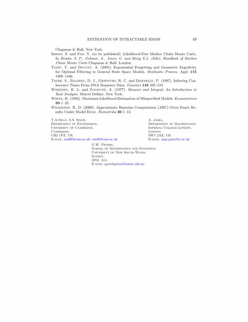
ESTIMATION OF INTRACTABLE HMMS 49
Chapman & Hall, New York.Sisson, S. and Fan, Y. (to be published). Likelihood-Free Markov Chain Monte Carlo.
In Brooks, S. P., Gelman, A., Jones, G. and Meng X.L. (Eds); Handbook of MarkovChain Monte Carlo Chapman & Hall: London.
Tadic, V. and Doucet, A. (2005). Exponential Forgetting and Geometric Ergodicityfor Optimal Filtering in General State Space Models. Stochastic Process. Appl. 1151408–1436.
Tavre, S., Balding, D. J., Griffiths, R. C. and Donnelly, P. (1997). Inferring Coa-lescence Times From DNA Sequence Data. Genetics 145 505–518.
Wheeden, R. L. and Zygmund, A. (1977). Measure and Integral; An Introduction toReal Analysis. Marcel Dekker, New York.
White, H. (1982). Maximum Likelihood Estimation of Misspecified Models. Econometrica50 1–25.
Wilkinson, R. D. (2008). Approximate Bayesian Computation (ABC) Gives Exact Re-sults Under Model Error. Biometrika 20 1–13.
T.A.Dean, S.S. Singh,Department of Engineering,University of Cambridge,Cambridge,CB2 1PZ, UKE-mail: [email protected]; [email protected]
A. Jasra,Department of Mathematics,Imperial College London,London,SW7 2AZ, UKE-mail: [email protected]
G.W. Peters,School of Mathematics and Statistics,University of New South Wales,Sydney,2052, AusE-mail: [email protected]