Parameter-Constrained Adaptive Control †

Parameter-Constrained Adaptive Control†

W. D. Timmons,*,‡ H. J. Chizeck,§,| F. Casas,‡ V. Chankong,§ and P. G. Katona⊥

Wm Timmons & Associates, 513 Sill Avenue, Cuyahoga Falls, OH 44221, Departments of SystemsEngineering and Biomedical Engineering, Case Western Reserve University, Cleveland, Ohio 44106, and TheWhitaker Foundation, 1700 North Moore Street, Suite 2200, Rosslyn, Virginia 22209

Under certain conditions, parameter constraints that impose a priori information about the open-loop system can dramatically improve the performance of explicit adaptive controllers. Underother conditions, the constraints can actually decrease performance. First, this paper presentsa novel parameter-constrained identifier on the basis of an efficient, quadratic program solverapplied semirecursively, making it ideal for real-time adaptive control. Second, several usefullinear constraints for second-order ARMAX models are provided, along with a few examples oftheir development. Third, the algorithm and the constraints are applied to a benchmark modelto explore several conditions, summarized as six guidelines, under which parameter constraintsimprove or worsen adaptive control. In this last part, it is shown that common orthogonalprojection can produce poor results. It is also shown that a priori information is increasinglyvaluable as excitation decreases and that it is especially useful for adaptive control whencombined with re-identification techniques. These results are then applied to the pharmacologicalcontrol of a time-varying second-order ARMAX model of blood pressure.

1. Introduction

For systems that are time-varying or nonlinear, anadaptive controller based on a time series model (AR-MAX, CARIMA, NARMAX, etc.) may be a useful alter-native to a classical controller design, since little a prioriinformation is required. Ironically, the information thatis available is often discarded when an adaptive control-ler is used. As a result, the controller may need open-loop probing before initiating control; after initiation,it may be susceptible to gain and offset disturbances,temporary bursting, and other problems. If the a prioriknowledge were used instead of being discarded, theseproblems might be avoided or reduced. This idea is notnew; almost 20 years ago the imposition of exactinformation as equality constraints on one or more ofthe model parameters was shown to dramatically im-prove controller performance (Goodwin and Payne,1977). Others have since confirmed and refined thesefindings (Bai and Sastry, 1986; Chia et al., 1991; Claryand Franklin, 1984; Fletcher, 1987; Li, 1989; Zheng,1989; Dasgupta, 1986). Unfortunately, exactness israther restrictive, and so this approach is not widelyapplicable. Instead, most knowledge falls into the classof inequality constraints. An algorithm that imposesboth equality and inequality constraints would be moreuseful and have wider applicability. However, thesealgorithms are complicated and difficult to program.Probably for this reason, most studies on inequality-constrained identification for adaptive control are lim-ited to either the bounding of a few critical parameters(Goodwin and Sin, 1984) or the use of simplified,suboptimal algorithms with loose parameter bounds.

The latter includes the σ-modifiers (Ortega and Tang,1989), the radial contractors (Praly et al., 1989), andthe simple saturators (Goodwin and Sin, 1984). Thosestudies primarily address the related and importantissue of global asymptotic stability, which is not thesame as the practical use of a priori information asparameter constraints.While simplified algorithms and reduced constraint

sets often dramatically improve controller performance,it is shown below that they can sometimes decreasecontroller performance and even exacerbate temporarydisturbances. The possibility of poor behavior raisesconsiderable safety concerns for life-critical applicationssuch as the control of vital signs in hospital patients,chemotherapy veno-infusion, and anesthesia regulation,where temporary instabilities and poor transient re-sponses can be life-threatening. For these types ofapplications, it becomes important to understand howand when a priori information helps or hinders control-ler performance.The addition of mixed equality and inequality con-

straints to an adaptive controller creates a nonlinearsystem that sometimes exhibits unexpected behaviors.Since an analytic analysis would be difficult, an empiri-cal approach is used here to develop and demonstratesix guidelines for the safe and effective use of parameter-constrained adaptive control. First, however, equationsare developed for a novel identifier that imposes mixedequality and inequality constraints both optimally andsemirecursively, two key properties that make theidentifier attractive for real-time adaptive control.Since the equations form a quadratic program (QP), afast, compact, and novel QP algorithm is included inthe Appendix. Following the section on identifierdevelopment, the construction of several constraintsfrom commonly available a priori information is il-lustrated and then followed by the empirical analysis.The results of the analysis are then applied to thepharmacological control of a time-varying second-orderARMAX model of blood pressure.

† A preliminary version of this work was presented at the12th IFAC World Congress, July 18-23, 1993, Sydney, Aus-tralia.

‡ Wm Timmons & Associates.§ Department of Systems Engineering, Case Western Re-

serve University.| Department of Biomedical Engineering, Case Western

Reserve University.⊥ The Whitaker Foundation.

4894 Ind. Eng. Chem. Res. 1997, 36, 4894-4905

S0888-5885(96)00659-8 CCC: $14.00 © 1997 American Chemical Society

2. Problem Formulation

Consider a linear or pseudolinear model in predictorform:

where e(t) is a zero mean white noise sequence. Thisform includes a broad class of time series models(ARMAX, NARMAX, CARIMA, etc.). For example,given the discrete time ARMAX model

the vectors θ and O(t-1) may be defined as

2.1. The Unconstrained Estimates. For θ un-known, the exponentially weighted recursive leastsquares (RLS) estimate is (Goodwin and Sin, 1984):

where 0 < R(t) e 1 is a scalar forgetting factor, P(t - 1)is a matrix proportional to the inverted data covariancematrix, and the subscript f signifies that θ is the free,or unconstrained, solution. The RLS estimate mini-mizes the sum of the squared prediction errors:

where θ is the vector of unknown parameters to beestimated, W(t) is a diagonal matrix defined by theR(t), and

The equivalent nonrecursive solution is

2.2. The Optimal Projector. Now consider theminimization of (5) subject to the following linearequality and inequality constraints (a convex quadraticprogram):

The Lagrangian for this system is (Fletcher, 1987):

where µ and λ are vectors of Lagrange multipliersassociated with the equality and inequality constraints,respectively. For positive definite XTWX, or equiva-lently, positive definite P, the first-order Kuhn-Tuckerconditions are the necessary and sufficient conditionsfor a unique global minimum (Luenberger, 1984):

(dropping the time subscripts for convenience). Solving(14) for θ (which we denote as θc since it is theconstrained solution), we obtain

which is in the form of the unconstrained estimate pluscorrections due to the constraints. P and θf can becomputed from (4) or (7), depending on the speed andnumerical requirements: in applications in which timeis scarce (e.g., adaptive control), the recursive form ispreferred. All that remains is to determine the Lagrangemultipliers µ and λ, which must be performed in batchusing quadratic programming (hence the semirecursivenature of the identifier). Positive semidefinite comple-mentary linear programming (CLP) is a relatively fast,compact quadratic-programming technique similar tothe simplex algorithm for linear programming (Dantzigand Cottle, 1967; Golub and Saunders, 1970). Anenhanced version developed by Timmons (1992) specif-ically for real-time applications is described in theAppendix.A CLP for this problemmay be constructed as follows.

Define the slack variables σ and ν as the constrainterrors (K - Mθ) and (C - Lθ). Using (15), eliminate θcto obtain

with the conditions

Equations 16 and 17 form the CLP. Note that if thereare only equality constraints, the solution reduces to aclosed form:

2.3. The Orthogonal Projector. The solution (15)could also have been obtained by minimizing the costfunction

subject to the constraints in (8). In this formulation,the optimal (least squares) correction terms in (15)represent the P-weighted projection of θf onto the

y(t) ) OT(t-1)θ + e(t) (1)

y(t) ) a1y(t-1) + ... + any(t-n) + b1u(t-1) +... bmu(t-m) + e(t) (2)

θ ∆ [a1, ..., an, b1, ..., bm]T

O(t-1) ∆ [y(t-1), ..., y(t-n), u(t-1), ..., u(t-m)]T (3)

θf(t) ) θf(t-1) +

P(t-2)O(t-1)‚[y(t) - O(t-1)Tθf(t-1)]

r(t-1) + O(t-1)TP(t-2)O(t-1)

P(t-1) )

1r(t-1)

‚[P(t-2) -P(t-2)O(t-1)O(t-1)TP(t-2)

r(t-1) + O(t-1)TP(t-2)O(t-1)] (4)

J ) 1/2[Y(t) - X(t-1)θ]TW(t)[Y(t) - X(t-1)θ] (5)

Y(t) ∆ [y(1), y(2), ..., y(t)]T

X(t-1) ∆ [O(0)|O(1)| ... |O(t-1)]T (6)

θf(t) ) P(t-1)XT(t-1)W(t)Y(t)

P(t-1) ) [XT(t-1)W(t)X(t-1)]-1 (7)

Mθ ) K

Lθ e C (8)

L (θ,µ,λ) ) 1/2[Y(t) - X(t-1)θ]TW(t) ×[Y(t) - X(t-1)θ] - µT(K - Mθ) - λT(C - Lθ) (9)

K - Mθ ) 0 (10)

C - Lθ g 0 (11)

λ g 0 (12)

λT(C - Lθ) ) 0 (13)

-XTW(Y - Xθ) + MTµ + LTλ ) 0 (14)

θc ) θf - PMTµ - PLTλ (15)

[σν ] ) [MPMT MPLT

LPMT LPLT ][µλ ] + [K - Mθf

C - Lθf ] (16)

σ ) 0, ν g 0, λ g 0

σTµ + νTλ ) 0 (17)

µ ) (MPMT)-1(Mθf - K)

(λ ) L) (18)

Jproj ) 1/2[θ - θf]TP-1[θ - θf] (19)

Ind. Eng. Chem. Res., Vol. 36, No. 11, 1997 4895

constraint surface. By replacing P with the identitymatrix, an orthogonal projector is obtained. Assumingthe constraints are true, parameter bias can never beincreased with this algorithm, which is something thatcannot be said for the optimal projector (Chia, 1991).The orthogonal projector can often be greatly simpli-

fied. For example, when the constraints consist ofindividual parameter bounds only, the orthogonal pro-jector reduces to a saturator:

and when the constraints are in the form of a sphere, itreduces to a radial contractor

where θ0 is the center of the sphere and F is its radius.The orthogonal projector thus has a seeming advantageover the optimal projector. This is discussed furtherbelow.

3. Armax Constraints

A range on steady-state gain and settling time, anapproximate pole or zero location, and the sign of oneor more parameters are often known. Classificationssuch as “open-loop stable” or “well-damped” also conveyuseful information. Linear ARMAX constraints thatimpose this type of information are listed in Table 1.While some constraints are general, for clarity and

simplicity, most are targeted toward the common,second-order ARMAX model. Many of the constraintsrely on the Jury criteria for the sign of 1 - Σai and hencerequire stability. For unstable systems, the constraintsmust be reformulated. These modifications, as well asextensions to other model forms, are mostly straight-forward. In the following, constraint development isbriefly illustrated and then followed by an elaborationon several of the more complicated constraints in Table1.3.1. Example of Constraint Development:

Steady-State Gain. Since steady-state gain is onlydefined for stable systems, open-loop stability must alsobe imposed on the estimates. From eq (2), Gss may becalculated as

For Gssmin e Gss e Gssmax, we obtain two inequalityconstraints, which can be put into linear (in θ) form onlyif the sign of 1 - Σai is known. By the Jury criteria,the sign must be positive, resulting in entry 3 in Table1.3.2. Steady-State Points. A steady-state point

(SSP) is a known steady-state input/output pair associ-ated with the model. Often the background level (thesteady-state unforced output) is known. Sometimesanother point, such as an equilibrium point for achemical reaction, is also known. For many systems,these points drift. For nonlinear systems, these pointsmay appear to drift due to linearization and hence mayrange farther than anticipated. In such systems, thesepoints may better be regarded as free or slack variables

Table 1. ARMAX Constraints from Commonly Available a Priori Knowledgea

knowledge constraint comments

1 individual parameters θimin e θi e θimax2 second-order open-loop stability a1 + a2 e 1

-a1 + a2 e 1-a2 e 1

3 steady-state gain: Gssmin e Gss e Gssmax Σbi + Gssmin Σai g Gssmin Use only with constrained open-loop stableΣbi + Gssmax Σai e Gssmax systems. Do not use with entry 5.

4 one SSP: (U1,Y1) yj(t) ∆ y(t) - Y1 Use yj and uj to estimate a and b parameters.uj(t) ∆ u(t) - U1 This approach is equivalent to, but more

efficient than, an equality constraint.5 two SSP’s: (U1,Y1), (U2,Y2) Y2 - Y1 ) (Y2 - Y1)Σai + (U2 - U1)Σbi Imposes a steady-state gain. Use in conjunction

with entry 4, but in place of entry 3.6 one SSP range: (U1,Ymin) to (U1,Ymax) (1 - Σai)Ymin g (Σbi)U1 + D See text for explanation of D.

(1 - Σai)Ymax e (Σbi)U1 + D7 one SSP range: (U1,Ymin) to (U1,Ymax) A(q-1)(ylp(t) - Ymin) e B(q-1)(ulp(t) - U1) A(q-1) and B(q-1) is standard ARMAX notation.

A(q-1)(ylp(t) - Ymax) g B(q-1)(ulp(t) - U1) Subscript lp indicates low-pass filtering;high-pass filtered data is used to estimateparameters. Noise may invalidate constraints.See text.

8 open-loop settling time ra1 + a2 e r2 r ) exp(-4.6T/τs), where T is the sampling interval(second-order systems) -ra1 + a2 e r2 and τs is the settling time.

-a2 e r29 min and max settling time -rmax

2 a1 + (rmin - 2rmax)a2 e -rmax2 rmin Only applies to sampled, continuous time systems

(certain second-order systems) rmaxa1 + a2 e rmax2 with real poles. rmin and rmax are the radii

a2 e 0 associated with the minimum and maximumsettling times.

10 open-loop minimum phase zeros sgn(b1)(b1rz2 + b2rz + b3) g 0 For stable second-order systems, b1 has the same

(second-order systems) sgn(b1)(b1rz2 - b2rz + b3) g 0 sign as Gss. rz ) maximum radius of zeros (e1).

sgn(b1)(b1rz2 - b3) g 0

11 minimum phase noise polynomials -rnc1 - c2 e rn2 rn ) maximum radius of the noise polynomial roots (e1).

(second-order systems) rnc1 - c2 e rn2

c2 e rn2

a See Timmons (1992) for detailed derivations.

θci ) {θimin if θfi < θiminθfi if θimin e θfi e θimaxθimax if θfi > θimax

∀i (20)

θc ) {θf if |θf - θ0| e F

θ0 + Fθf - θ0

|θf - θ0|otherwise

(21)Gss )

∑i

bi

1 - ∑i

ai

(22)

4896 Ind. Eng. Chem. Res., Vol. 36, No. 11, 1997

that impart integral action into the estimator and itscoupled controller. Nevertheless, with care, a specifiedrange may be advantageous. Several approaches aresummarized in Table 1. They are briefly describedbelow.ARIMA- and CARIMA-type approaches estimate the

parameters using incremental outputs and inputsy∆(t) and u∆(t), defined as

where d is an arbitrary constant such as the systemdead time. By using this method, offsets are implicitlyremoved. Because of this formulation, a known SSP orits range is not easily imposed on the identification(though two SSP’s and their ranges can be imposed asconstraints on steady-state gain using Table 1, entry5). If instead, an offset term D were added to the rightside of eq (2), linear inequality constraints for the rangeof D may be formed with knowledge of the sign of1 - Σai. If the system is open-loop stable (and the modelis constrained as such), then the sign will be positive,and the constraint in Table 1, entry 6 may be used. Thefloating identifier (FI), described in Timmons et al.(1991), is another, related approach. It high pass orband pass filters the outputs and inputs: offsets areremoved for dynamics estimation and then added backfor offset estimation. As before, if the model is con-strained to be open-loop stable, then we arrive at asimilar set of inequality constraints (entry 7, Table 1).However, the constraints now depend on recent input/output data so that noise may invalidate them; hence,one must use care when imposing them.3.3. Open-Loop Settling Time. Settling time, the

time required for a step response to settle to within aband of its final value (e.g., (1%), is commonly known.

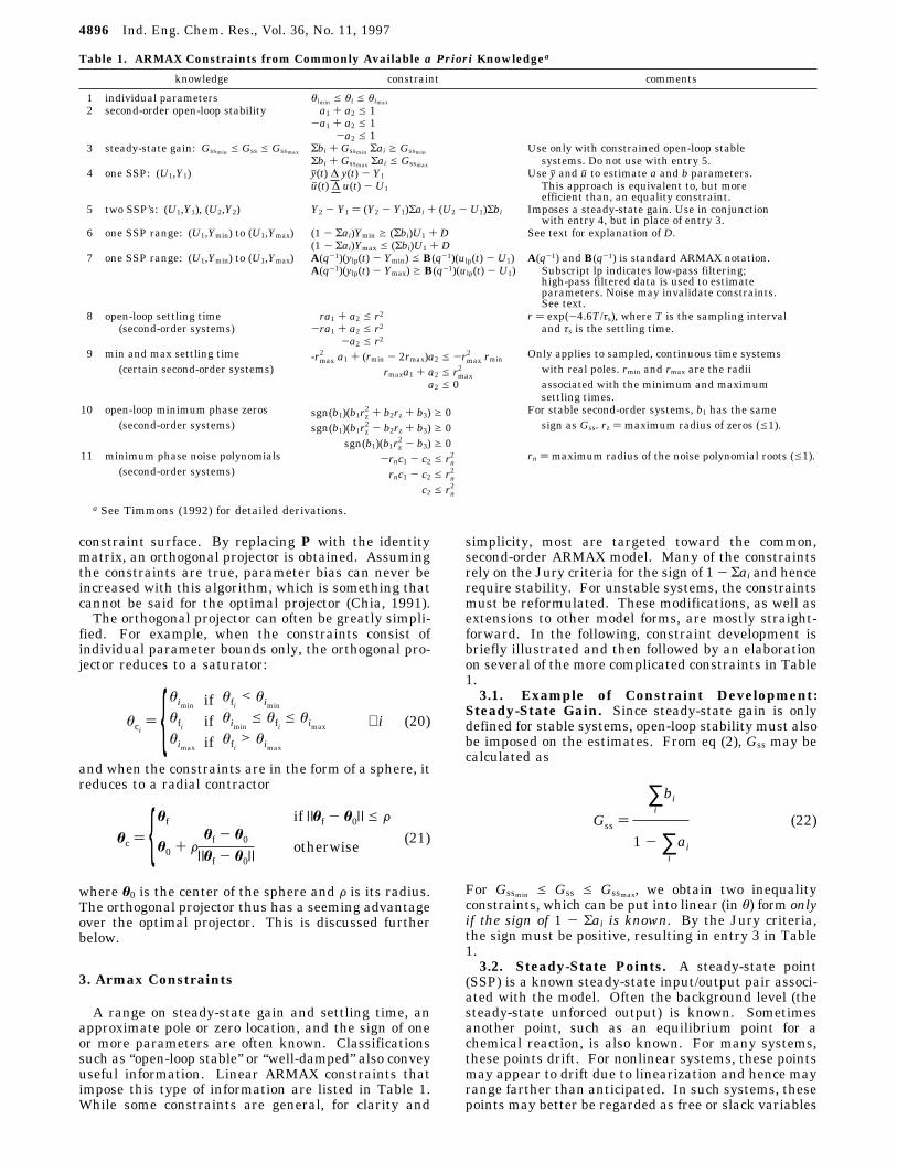
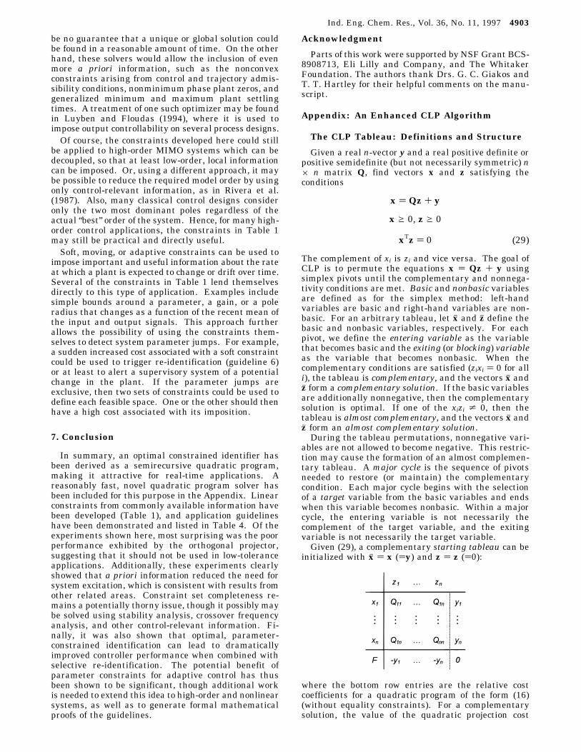
For second-order discrete time systems, a known maxi-mum settling time τs approximately translates to allpoles lying within a circle centered at the origin in theZ-plane with radius r ) exp(-4.6T/τs), where T is thesampling interval (Franklin and Powell, 1980, pp 100-103).Consider two poles, p1 and p2, with magnitude less

than r as in Figure 1a. Let pj1 ) p1/r and pj2 ) p2/r. Inthis new coordinate system, the original circle of radiusr corresponds to the unit circle (Figure 1b). We candirectly apply the stability constraints of Table 1 (entry2) to the transformed system (Figure 1c):

For second-order model structures similar to eq (2),

and

As shown in Figure 1d, we obtain the constraintslisted in entry 8 of Table 1.3.4. Example of Constraints Built on Other

Constraints: Open-Loop Zeros. The zeroes of mini-mum phase systems often lie within the unit circle inthe Z-plane. For a second-order ARMAX-type model,

Figure 1. Settling time conditions for second-order systems: (a) poles restricted to circle of radius r (<1); (b) transformed system polesare now restricted to the unit disc; (c) stability conditions for the transformed system; (d) inverse-transformed stability conditions resultin settling time conditions.

y∆(t) ∆ y(t) - y(t-d)

u∆(t) ∆ u(t) - u(t-d) (23)

aj1 + aj2 e 1

-aj1 + aj2 e 1

-aj2 e 1 (24)

a1 ) p1 + p2

a2 ) -p1p2 (25)

aj1 ) pj1 + pj2 ) (p1 + p2)/r ) a1/r

aj2 ) -pj1pj2 ) -p1p2/r2 ) a2/r

2 (26)


the B(q-1) polynomial (assuming a d-step delay) is givenby

In this form, we can utilize the constraints for settlingtime (entry 8, Table 1) with a1 and a2 replaced by -b2/b1 and -b3/b1. The radius r < 1 now specifies themaximum radius of the zeros. For stable systems, wecan convert these constraints to linear in θ form (entry10, Table 1) by recognizing that b1 has the same signasGss (Timmons, 1992). A similar approach can be usedfor second-order minimum phase noise polynomials(entry 11, Table 1).3.5. Example of Constraint Combinations. When

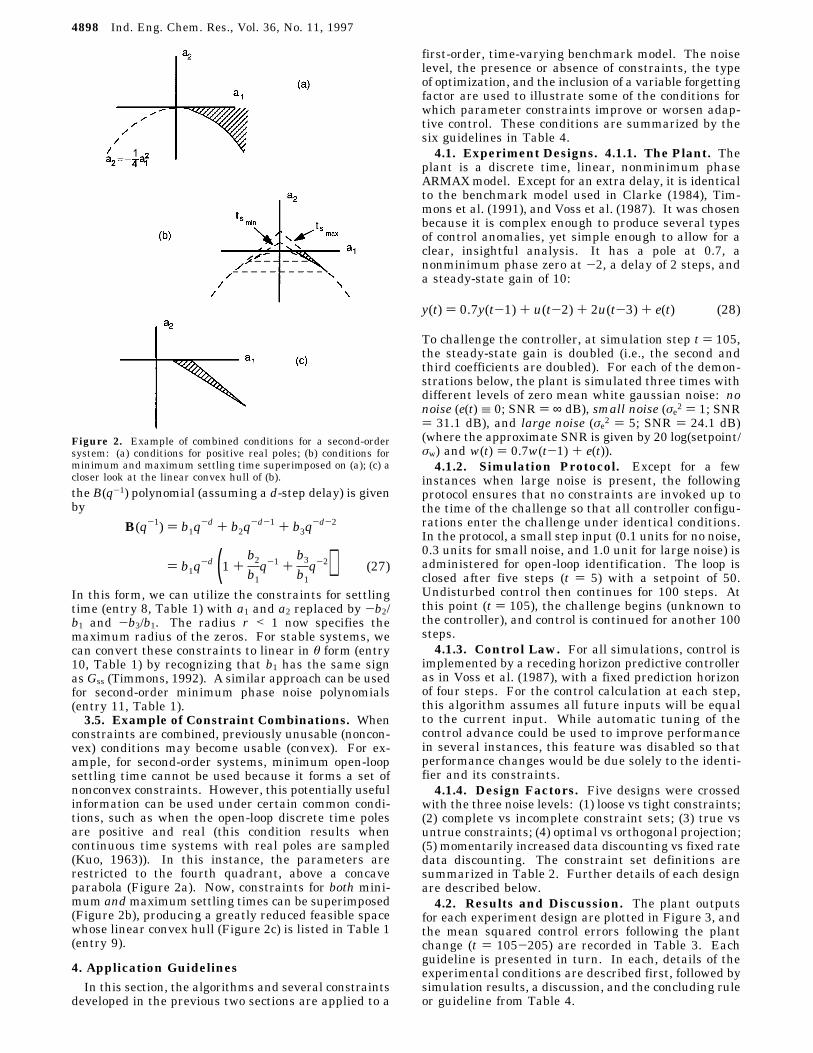
constraints are combined, previously unusable (noncon-vex) conditions may become usable (convex). For ex-ample, for second-order systems, minimum open-loopsettling time cannot be used because it forms a set ofnonconvex constraints. However, this potentially usefulinformation can be used under certain common condi-tions, such as when the open-loop discrete time polesare positive and real (this condition results whencontinuous time systems with real poles are sampled(Kuo, 1963)). In this instance, the parameters arerestricted to the fourth quadrant, above a concaveparabola (Figure 2a). Now, constraints for both mini-mum andmaximum settling times can be superimposed(Figure 2b), producing a greatly reduced feasible spacewhose linear convex hull (Figure 2c) is listed in Table 1(entry 9).

4. Application GuidelinesIn this section, the algorithms and several constraints

developed in the previous two sections are applied to a

first-order, time-varying benchmark model. The noiselevel, the presence or absence of constraints, the typeof optimization, and the inclusion of a variable forgettingfactor are used to illustrate some of the conditions forwhich parameter constraints improve or worsen adap-tive control. These conditions are summarized by thesix guidelines in Table 4.4.1. Experiment Designs. 4.1.1. The Plant. The

plant is a discrete time, linear, nonminimum phaseARMAXmodel. Except for an extra delay, it is identicalto the benchmark model used in Clarke (1984), Tim-mons et al. (1991), and Voss et al. (1987). It was chosenbecause it is complex enough to produce several typesof control anomalies, yet simple enough to allow for aclear, insightful analysis. It has a pole at 0.7, anonminimum phase zero at -2, a delay of 2 steps, anda steady-state gain of 10:

To challenge the controller, at simulation step t ) 105,the steady-state gain is doubled (i.e., the second andthird coefficients are doubled). For each of the demon-strations below, the plant is simulated three times withdifferent levels of zero mean white gaussian noise: nonoise (e(t) ≡ 0; SNR ) ∞ dB), small noise (σe2 ) 1; SNR) 31.1 dB), and large noise (σe2 ) 5; SNR ) 24.1 dB)(where the approximate SNR is given by 20 log(setpoint/σw) and w(t) ) 0.7w(t-1) + e(t)).4.1.2. Simulation Protocol. Except for a few

instances when large noise is present, the followingprotocol ensures that no constraints are invoked up tothe time of the challenge so that all controller configu-rations enter the challenge under identical conditions.In the protocol, a small step input (0.1 units for no noise,0.3 units for small noise, and 1.0 unit for large noise) isadministered for open-loop identification. The loop isclosed after five steps (t ) 5) with a setpoint of 50.Undisturbed control then continues for 100 steps. Atthis point (t ) 105), the challenge begins (unknown tothe controller), and control is continued for another 100steps.4.1.3. Control Law. For all simulations, control is

implemented by a receding horizon predictive controlleras in Voss et al. (1987), with a fixed prediction horizonof four steps. For the control calculation at each step,this algorithm assumes all future inputs will be equalto the current input. While automatic tuning of thecontrol advance could be used to improve performancein several instances, this feature was disabled so thatperformance changes would be due solely to the identi-fier and its constraints.4.1.4. Design Factors. Five designs were crossed

with the three noise levels: (1) loose vs tight constraints;(2) complete vs incomplete constraint sets; (3) true vsuntrue constraints; (4) optimal vs orthogonal projection;(5) momentarily increased data discounting vs fixed ratedata discounting. The constraint set definitions aresummarized in Table 2. Further details of each designare described below.4.2. Results and Discussion. The plant outputs

for each experiment design are plotted in Figure 3, andthe mean squared control errors following the plantchange (t ) 105-205) are recorded in Table 3. Eachguideline is presented in turn. In each, details of theexperimental conditions are described first, followed bysimulation results, a discussion, and the concluding ruleor guideline from Table 4.

Figure 2. Example of combined conditions for a second-ordersystem: (a) conditions for positive real poles; (b) conditions forminimum and maximum settling time superimposed on (a); (c) acloser look at the linear convex hull of (b).

B(q-1) ) b1q-d + b2q

-d-1 + b3q-d-2

) b1q-d (1 +

b2b1q-1 +

b3b1q-2) (27)

y(t) ) 0.7y(t-1) + u(t-2) + 2u(t-3) + e(t) (28)


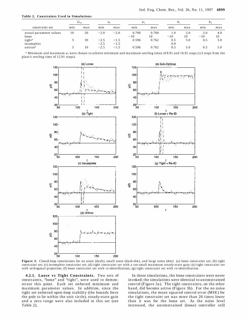
4.2.1. Loose vs Tight Constraints. Two sets ofconstraints, “loose” and “tight”, were used to demon-strate this point. Each set enforced minimum andmaximum parameter values. In addition, since thetight set enforced open-loop stability (the bounds forcethe pole to lie within the unit circle), steady-state gainand a zero range were also included in this set (seeTable 2).

In these simulations, the loose constraints were neverinvoked; the simulations were identical to unconstrainedcontrol (Figure 3a). The tight constraints, on the otherhand, did become active (Figure 3b). For the no noisesimulations, the mean squared control error (MSE) forthe tight constraint set was more than 26 times lowerthan it was for the loose set. As the noise levelincreased, the unconstrained (loose) controller still

Table 2. Constraints Used in Simulations

Gss z0 a1 b1 b2

constraint set min max min max min max min max min max

actual parameter values 10 20 -2.0 -2.0 0.700 0.700 1.0 2.0 2.0 4.0loose -10 10 -10 10 -10 10tighta 5 30 -2.5 -1.5 0.596 0.762 0.5 5.0 0.5 5.0incomplete -2.5 -1.5 0.0untruea 5 10 -2.5 -1.5 0.596 0.762 0.5 5.0 0.5 5.0a Minimum and maximum a1 were chosen to achieve minimum and maximum settling times of 8.91 and 16.91 steps ((3 steps from the

plant’s settling time of 12.91 steps).

Figure 3. Closed-loop simulations for no noise (dash), small noise (dash-dot), and large noise (dot): (a) loose constraint set; (b) tightconstraint set; (c) incomplete constraint set; (d) tight constraint set with a too small maximum steady-state gain; (e) tight constraint setwith orthogonal projection; (f) loose constraint set with re-identification; (g) tight constraint set with re-identification.


exhibited instability at the plant change, though itsoverall MSE improved. The constrained (tight) control-ler only slightly worsened (Table 3). Eventually, for alarge enough excitation, the a priori information wouldhave provided little additional benefit.Thus, the rule here is constraints should be tight

enough to be invoked. That is, if we want a performanceimprovement using constraints, the bounds must betight enough that they will become active at some time.A second rule can also be stated: a priori informationbecomes increasingly important as excitation decreases.This last rule is very important considering that mostregulators try to achieve zero excitation.4.2.2. Complete vs Incomplete Constraint Set.

In this example, several of the constraints in theprevious example were eliminated. When using mini-mum variance adaptive control, it is common to boundthe sign of b1 or fix it within a range of values so as toenforce stability (A° strom and Wittenmark, 1973; Lo-zano-Leal and Collado, 1989). For extended and reced-ing horizon control laws, however, b1 is no longer theonly important parameter (Egardt, 1980; Elliott, 1982;Lozano-Leal and Collado, 1989). Here, only the sign ofb1 and a range for the zero are enforced (see Table 2).In this simulation, the reduced constraints did not

eliminate the instability when the plant changed (Fig-ure 3c), although for the no noise case they did decreasethe input and output excursions compared to theunconstrained case. For the small noise case, the MSEwith these constraints was worse than it was for noconstraints (see Table 3).In general, we have found that if only one part of a

model is constrained, then the modeling error may beexaggerated in another. If the controller is sensitive toerrors in the unconstrained part of the plant, thencontroller performance may suffer, sometimes morethan if no constraints had been used. This raises thequestions, should some types of information be ignored,or is there some way to complete the information set sothat this problem does not occur? While these questionsremain the topic of future research, constraints thatenforce the global asymptotic stability conditions maysuffice. For example, we have found that since recedingand extended horizon control laws are sensitive to thelocation of plant zeros, constraints on the zeros oftenovercome this problem. Furthermore, the results fromEskinat et al. (1993) suggest that modeling the systemaround its crossover frequency might help generate thecritical missing information. Also, as in Kwong et al.(1995), focusing on the control-relevant informationshould help address this issue. For now, however, thecompleteness issue remains a potentially serious draw-back for life-critical applications. While it may bedifficult to implement, the rule here is the constraintset should be complete.4.2.3. True vs Untrue Constraints. In this ex-

ample, the set of tight constraints in the first examplewas modified to impose too small of an upper limit on

the steady-state gain. Although temporary instabilitywas eliminated at the plant change, a constant steady-state error remained (Figure 3d). The sum of thesquared errors would have continued to accumulate overtime; eventually the MSE would have been larger forthis case than for any of the previous examples. Thus,the rule here becomes untrue constraints degrade per-formance. While this rule may seem trivial and obvious,it is important because it is easily and unsuspectinglyviolated, especially when linear approximations are usedfor nonlinear plants.4.2.4. Optimal vs Orthogonal Projection. In all

previous simulations, the optimal (least squares) esti-mates were used. In this example (Figure 3e), thesimulation experiment in Figure 3b (the tight set ofconstraints) is repeated with the orthogonal projectorin place of the optimal projector. Here, just like theoptimal projector (Figure 3b), the instability was elimi-nated. Unlike the optimal projector, however, a steady-state error remained. As in the example with theincorrect constraint (Figure 3d), the sum of the squarederrors would have continued to increase linearly withtime. Moreover, this steady-state error (Figure 3e) waslarger at all noise levels than it was with the untrueconstraint (Figure 3d). Application of the orthogonalprojector to the other experiment designs of this studyprovided no additional information and so are notincluded here. However, in our experience with othermodels, the orthogonal projector occasionally impairedtransient stability too.The question might be asked, “Is performance worth

trading for algorithm simplicity?” There are threeresponses. First, in this experiment, since the con-straints do not form a set of simple bounds or a simplehypersphere, the orthogonal projector does not reduceto an attractive, simple algorithm, but remains ascomplex as the optimal projector. Second, simplicitycould be regained if the constraints were relaxed to aconvex hull made up of simple bounds or a hypersphere(potentially ignoring some useful a priori information),but then guideline 1 (Table 4) would be violated,potentially causing further degradation. Third, even ifa simple algorithm could be used, the performance (asshown in this experiment) would still be unacceptablein life-critical applications. Thus, we conclude that theorthogonal projector is not a worthwhile substitute forthe optimal projector, even when the constraint spaceis simple, and especially when a high price may beattached to poor performance. Interestingly, there issome evidence that the orthogonal projector may actu-ally be a better choice when the P-matrix is poorlyconditioned, which would be consistent with the resultsin Chia et al. (1991). This is the topic of future research.With this caveat in mind, the rule here is use optimalprojection.4.2.5. Momentarily Increased Data Discounting

vs Fixed Rate Data Discounting. After a plantchange, data from the new plant must compete withdata from the old during system identification. There-fore, it is common to discard old data when a changehas been detected (Goodwin and Sin, 1984). The data

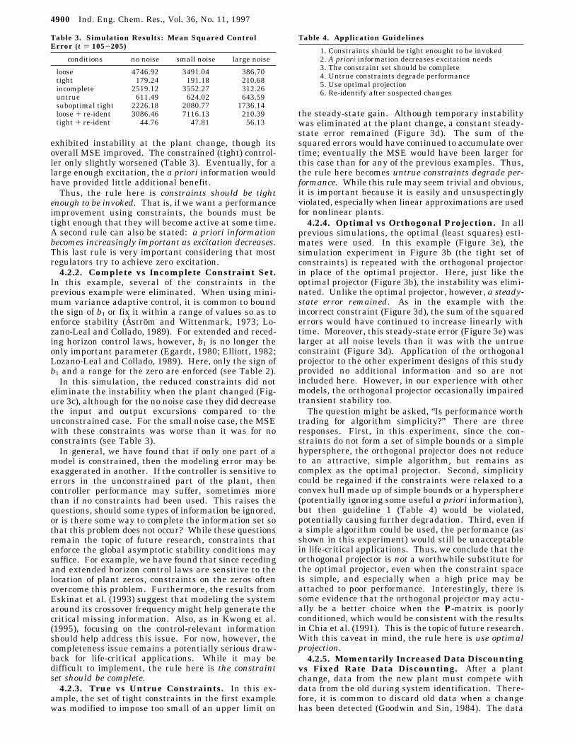
Table 3. Simulation Results: Mean Squared ControlError (t ) 105-205)

conditions no noise small noise large noise

loose 4746.92 3491.04 386.70tight 179.24 191.18 210.68incomplete 2519.12 3552.27 312.26untrue 611.49 624.02 643.59suboptimal tight 2226.18 2080.77 1736.14loose + re-ident 3086.46 7116.13 210.39tight + re-ident 44.76 47.81 56.13

Table 4. Application Guidelines

1. Constraints should be tight enought to be invoked2. A priori information decreases excitation needs3. The constraint set should be complete4. Untrue constraints degrade performance5. Use optimal projection6. Re-identify after suspected changes


can be discarded by either resetting the P-matrix(blanking past data) or increasing the speed of adapta-tion by lowering the estimator’s exponential forgettingfactor (rapidly discounting past data). In this nextexample, the past data is discounted by reducing theforgetting factor to 0.5 for five steps, then increasing itto 0.75 for eight steps, and finally returning it to itsoriginal value of 0.98. This approach is applied to theexperiment designs in Figures 3a (loose) and 3b (tight).Results are plotted in Figures 3f and 3g, respectively.Re-identification after the plant change when using

the loose set of constraints (Figure 3f) did not eliminatethe plant change instability. In fact, when small noisewas present, the input and output excursions werenearly twice as large as when re-identification was notused. However, the control error did go to zero im-mediately after the instability, unlike Figure 3a.When using the tight set of constraints, control

remained stable and the control error went to zerorapidly (Figure 3g). For the no noise case, the MSE wasreduced by more than a factor of 100 compared to theoriginal loose constraint example in Figure 3a. Fur-thermore, with the tight constraint set, the MSEincreased only slightly as the noise level increased (seeTable 3). Note that this trend still supports guideline2. More importantly, note that with appropriate pa-rameter constraints, the adaptation gain can seeminglybe increased without sacrificing stability. This suggeststhe final rule, re-identify after suspected changes.

5. Control of Second-Order Blood PressureArmax Model

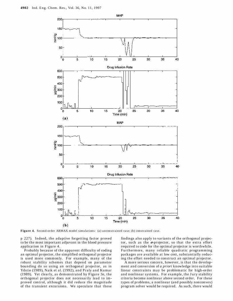
In this section the guidelines are applied to the controlof a simulated mean arterial blood pressure (MAP)model using a vasodilator (sodium nitroprusside, SNP).5.1. The ARMAX Model. In modeling the MAP/

SNP system, the y(t) in (2) represents the measuredMAP at time t, while u(t) corresponds to the SNPinfusion rate at time t. To form a time-varying ARMAXmodel, a before and an after model were defined. Thebefore model was obtained by probing a pentobarbital-anesthetized dog with SNP; the after model was ob-tained from the same dog following a disturbance causedby an unknown event which resulted in a 3-fold increasein the steady-state gain and a change in the base lineblood pressure (Timmons, 1992). The disturbance wasimplemented by ramping the exogenous input param-eters (the b’s) between the before (-0.072, 0.036) andafter (-0.216, 0.108) models, while maintaining theautoregressive terms (the a’s) fixed (-0.7, 0.06). Toobtain a resting MAP, base line levels of 150 mmHg forthe beforemodel and 111 mmHg for the aftermodel wereadded. In addition, a zero mean white Gaussian noisewith a variance of 0.25 mmHg2 was added to the processas in (28).5.2. Controller Setup and Simulation. For sys-

tem identification, a recursive least squares algorithmwith a variable forgetting factor was used. The identi-fied model assumed a 20 s sampling interval, twoautoregressive terms (a’s), and three exogenous inputterms (b’s) with an input/output delay of one sample.For the constrained identification, minimum and maxi-mum limits were imposed on the steady-state gain(-1.0, -0.04), the settling time (0.4, 0.7), and themagnitude of the zeros (0.7) (see Table 1, entries 3, 9,and 10). A receding horizon predictive controller witha prediction horizon of six samples (Voss, 1988) wasused to generate the SNP infusion rates.

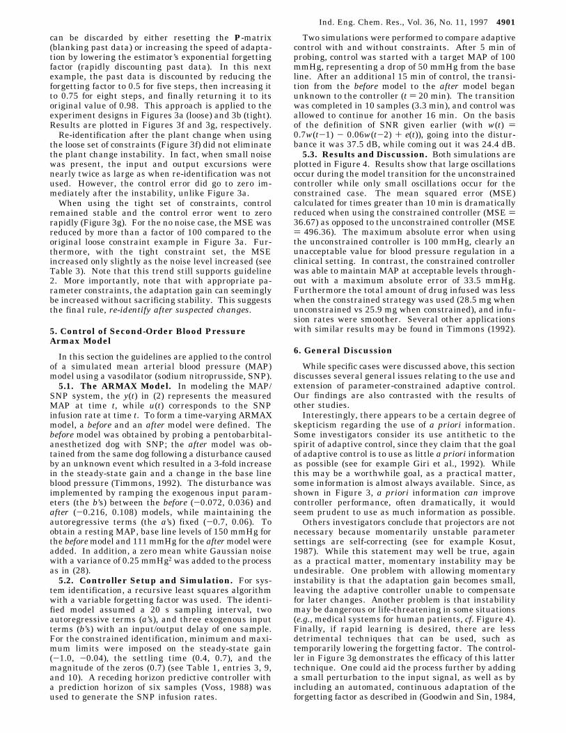
Two simulations were performed to compare adaptivecontrol with and without constraints. After 5 min ofprobing, control was started with a target MAP of 100mmHg, representing a drop of 50 mmHg from the baseline. After an additional 15 min of control, the transi-tion from the before model to the after model beganunknown to the controller (t ) 20 min). The transitionwas completed in 10 samples (3.3 min), and control wasallowed to continue for another 16 min. On the basisof the definition of SNR given earlier (with w(t) )0.7w(t-1) - 0.06w(t-2) + e(t)), going into the distur-bance it was 37.5 dB, while coming out it was 24.4 dB.5.3. Results and Discussion. Both simulations are

plotted in Figure 4. Results show that large oscillationsoccur during the model transition for the unconstrainedcontroller while only small oscillations occur for theconstrained case. The mean squared error (MSE)calculated for times greater than 10 min is dramaticallyreduced when using the constrained controller (MSE )36.67) as opposed to the unconstrained controller (MSE) 496.36). The maximum absolute error when usingthe unconstrained controller is 100 mmHg, clearly anunacceptable value for blood pressure regulation in aclinical setting. In contrast, the constrained controllerwas able to maintain MAP at acceptable levels through-out with a maximum absolute error of 33.5 mmHg.Furthermore the total amount of drug infused was lesswhen the constrained strategy was used (28.5 mg whenunconstrained vs 25.9 mg when constrained), and infu-sion rates were smoother. Several other applicationswith similar results may be found in Timmons (1992).

6. General Discussion

While specific cases were discussed above, this sectiondiscusses several general issues relating to the use andextension of parameter-constrained adaptive control.Our findings are also contrasted with the results ofother studies.Interestingly, there appears to be a certain degree of

skepticism regarding the use of a priori information.Some investigators consider its use antithetic to thespirit of adaptive control, since they claim that the goalof adaptive control is to use as little a priori informationas possible (see for example Giri et al., 1992). Whilethis may be a worthwhile goal, as a practical matter,some information is almost always available. Since, asshown in Figure 3, a priori information can improvecontroller performance, often dramatically, it wouldseem prudent to use as much information as possible.Others investigators conclude that projectors are not

necessary because momentarily unstable parametersettings are self-correcting (see for example Kosut,1987). While this statement may well be true, againas a practical matter, momentary instability may beundesirable. One problem with allowing momentaryinstability is that the adaptation gain becomes small,leaving the adaptive controller unable to compensatefor later changes. Another problem is that instabilitymay be dangerous or life-threatening in some situations(e.g., medical systems for human patients, cf. Figure 4).Finally, if rapid learning is desired, there are lessdetrimental techniques that can be used, such astemporarily lowering the forgetting factor. The control-ler in Figure 3g demonstrates the efficacy of this lattertechnique. One could aid the process further by addinga small perturbation to the input signal, as well as byincluding an automated, continuous adaptation of theforgetting factor as described in (Goodwin and Sin, 1984,


p 227). Indeed, the adaptive forgetting factor provedto be the most important adjuvant in the blood pressureapplication in Figure 4.Probably because of the apparent difficulty of coding

an optimal projector, the simplified orthogonal projectoris used more commonly. For example, many of therobust stability schemes that depend on parameterbounding do so using an orthogonal projector, as inYdstie (1989), Naik et al. (1992), and Praly and Kumar(1989). Yet clearly, as demonstrated by Figure 3e, theorthogonal projector does not necessarily lead to im-proved control, although it did reduce the magnitudeof the transient excursions. We speculate that these

findings also apply to variants of the orthogonal projec-tor, such as the σ-projector, so that the extra effortrequired to code for the optimal projector is worthwhile.Furthermore, many reliable quadratic programmingpackages are available at low cost, substantially reduc-ing the effort needed to construct an optimal projector.A more serious concern, however, is that the develop-

ment and conversion of a priori knowledge into suitablelinear constraints may be problematic for high-orderand nonlinear systems. For example, the Jury stabilitycriteria become nonlinear above second order. For thesetypes of problems, a nonlinear (and possibly nonconvex)program solver would be required. As such, there would

Figure 4. Second-order ARMAX model simulations: (a) unconstrained case; (b) constrained case.


be no guarantee that a unique or global solution couldbe found in a reasonable amount of time. On the otherhand, these solvers would allow the inclusion of evenmore a priori information, such as the nonconvexconstraints arising from control and trajectory admis-sibility conditions, nonminimum phase plant zeros, andgeneralized minimum and maximum plant settlingtimes. A treatment of one such optimizer may be foundin Luyben and Floudas (1994), where it is used toimpose output controllability on several process designs.Of course, the constraints developed here could still

be applied to high-order MIMO systems which can bedecoupled, so that at least low-order, local informationcan be imposed. Or, using a different approach, it maybe possible to reduce the required model order by usingonly control-relevant information, as in Rivera et al.(1987). Also, many classical control designs consideronly the two most dominant poles regardless of theactual “best” order of the system. Hence, for many high-order control applications, the constraints in Table 1may still be practical and directly useful.Soft, moving, or adaptive constraints can be used to

impose important and useful information about the rateat which a plant is expected to change or drift over time.Several of the constraints in Table 1 lend themselvesdirectly to this type of application. Examples includesimple bounds around a parameter, a gain, or a poleradius that changes as a function of the recent mean ofthe input and output signals. This approach furtherallows the possibility of using the constraints them-selves to detect system parameter jumps. For example,a sudden increased cost associated with a soft constraintcould be used to trigger re-identification (guideline 6)or at least to alert a supervisory system of a potentialchange in the plant. If the parameter jumps areexclusive, then two sets of constraints could be used todefine each feasible space. One or the other should thenhave a high cost associated with its imposition.

7. Conclusion

In summary, an optimal constrained identifier hasbeen derived as a semirecursive quadratic program,making it attractive for real-time applications. Areasonably fast, novel quadratic program solver hasbeen included for this purpose in the Appendix. Linearconstraints from commonly available information havebeen developed (Table 1), and application guidelineshave been demonstrated and listed in Table 4. Of theexperiments shown here, most surprising was the poorperformance exhibited by the orthogonal projector,suggesting that it should not be used in low-toleranceapplications. Additionally, these experiments clearlyshowed that a priori information reduced the need forsystem excitation, which is consistent with results fromother related areas. Constraint set completeness re-mains a potentially thorny issue, though it possibly maybe solved using stability analysis, crossover frequencyanalysis, and other control-relevant information. Fi-nally, it was also shown that optimal, parameter-constrained identification can lead to dramaticallyimproved controller performance when combined withselective re-identification. The potential benefit ofparameter constraints for adaptive control has thusbeen shown to be significant, though additional workis needed to extend this idea to high-order and nonlinearsystems, as well as to generate formal mathematicalproofs of the guidelines.

Acknowledgment

Parts of this work were supported by NSF Grant BCS-8908713, Eli Lilly and Company, and The WhitakerFoundation. The authors thank Drs. G. C. Giakos andT. T. Hartley for their helpful comments on the manu-script.

Appendix: An Enhanced CLP Algorithm

The CLP Tableau: Definitions and Structure

Given a real n-vector y and a real positive definite orpositive semidefinite (but not necessarily symmetric) n× n matrix Q, find vectors x and z satisfying theconditions

The complement of xi is zi and vice versa. The goal ofCLP is to permute the equations x ) Qz + y usingsimplex pivots until the complementary and nonnega-tivity conditions are met. Basic and nonbasic variablesare defined as for the simplex method: left-handvariables are basic and right-hand variables are non-basic. For an arbitrary tableau, let xj and zj define thebasic and nonbasic variables, respectively. For eachpivot, we define the entering variable as the variablethat becomes basic and the exiting (or blocking) variableas the variable that becomes nonbasic. When thecomplementary conditions are satisfied (zixi ) 0 for alli), the tableau is complementary, and the vectors xj andzj form a complementary solution. If the basic variablesare additionally nonnegative, then the complementarysolution is optimal. If one of the xizi * 0, then thetableau is almost complementary, and the vectors xj andzj form an almost complementary solution.During the tableau permutations, nonnegative vari-

ables are not allowed to become negative. This restric-tion may cause the formation of an almost complemen-tary tableau. A major cycle is the sequence of pivotsneeded to restore (or maintain) the complementarycondition. Each major cycle begins with the selectionof a target variable from the basic variables and endswhen this variable becomes nonbasic. Within a majorcycle, the entering variable is not necessarily thecomplement of the target variable, and the exitingvariable is not necessarily the target variable.Given (29), a complementary starting tableau can be

initialized with xj ) x ()y) and z ) z ()0):

where the bottom row entries are the relative costcoefficients for a quadratic program of the form (16)(without equality constraints). For a complementarysolution, the value of the quadratic projection cost

x ) Qz + y

x g 0, z g 0

xTz ) 0 (29)

F


function (19) is 1/2F (where F is the lower right entry inthe tableau). For an almost complementary solution,the value of the cost function is 1/2(F + xjTzj) (Timmons,1992).

The Enhanced CLP Algorithm

Step 0. Initialize tableau.Step 1. Start major cycle.S ) the set {xi | xi < 0, i ) 1, ..., n} /*S is the set ofpotential target variables*/

Step 2. Find target variable.If (xj g 0) thenReturn with solution /*Solution is optimal*/

Else if (S ) L) thenReturn with error /*No solution*/

ElseTarget ) xji, where xji ∈ S and yji2/Qh ii is maximum

EndifStep 3. Find entering variable. /*i.e., find the pivotcolumn*/If (tableau is complementary) thenEntering variable ) complement of target

ElseEntering variable ) complement of previous block-ing variable

EndifStep 4. Find exiting variable. /*i.e., find the pivot row*//*A block occurs when, upon increasing the enteringvariable, (a) the target variable increases to zero or(b) another basic variable decreases to zero*/If (blocked) thenblocking variable ) first variable to block/*Ties go to the target variable, if involved.Otherwise, resolve degeneracies using Charnes’smethod (e.g., see Luenberger, 1984)*/

Else if (tableau is complementary) thenRemove the target from S /*No block, so rejecttarget*/Goto to Step 2

ElseReturn with error /*No solution*/

EndifStep 5. Pivot.Exchange the entering variable for the blockingvariable

Step 6. Loop back.If (tableau is complementary) thenGoto Step 1 /*The major cycle ends*/

ElseGoto Step 3 /*The major cycle continues*/

EndifOur modifications to the original algorithm are (a) the

least distance target selection rule in Step 2 and (b) thetarget rejection rule in Step 4. See Timmons (1992) fordetails.

Equality Constraints

For numerical robustness, any equality constraintsthat are present should be included in the tableau (asin eq 16) (see Golub and Saunders, 1970). TheirLagrange multipliers and constraint errors should bemade basic and nonbasic, respectively (thus driving the

constraint errors to zero), and then removed from thelist of possible pivots.

Literature Cited

A° strom, K. J.; Wittenmark, B. On self-tuning regulators. Auto-matica 1973, 9, 185-199.

Bai, E.-W.; Sastry, S. S. Discrete Time Adaptive Control UtilizingPrior Information. IEEE Trans. Autom. Control 1986, 31, 779-782.

Chia, T. L.; Chow, P.-C.; Chizeck, H. J. Recursive ParameterIdentification of Constrained Systems: An Application toElectrically Stimulated Muscle. IEEE Trans. Biomed. Eng.1991, 38, 429-442.

Clarke, D. W. Self-tuning Control of Nonminimum-phase Systems.Automatica 1984, 20, 501-517.

Clary, J. P.; Franklin, G. F. Self-tuning Control with A Priori PlantKnowledge. Proceedings of the 23rd IEEE Conference onDecision and Control, Las Vegas, NV, 1984; IEEE: New York,1984; pp 369-374.

Dantzig, G. B.; Cottle, R. W. Positive (Semi-) Definite Program-ming. Nonlinear Programming; Abadie, J., Ed.; North-HollandPublishing Co.: Amsterdam (John Wiley and Sons, Inc.: NewYork), 1967; pp 55-73.

Dasgupta, S.; Anderson, B. D. O.; Kaye, R. J. Output ErrorIdentification of Partially Known Systems. Int. J. Control 1986,43, 177-191.

Egardt, B. Stability Analysis of Discrete-Time Adaptive ControlSchemes. IEEE Trans. Autom. Control 1980, 25, 710-716.

Elliott, H. Hybrid Adaptive Control of Continuous Time Systems.IEEE Trans. Autom. Control 1982, 27, 419-426.

Eskinat, E.; Johnson, S. H.; Luyben, W. L. Use of AuxiliaryInformation in System Identification. Ind. Eng. Chem. Res.1993, 32, 1981-1992.

Fletcher, R. Practical Methods of Optimization, 2nd ed. JohnWiley& Sons: New York, 1987.

Franklin, G. F.; Powell, J. D. Digital Control of Dynamic Systems.Addison-Wesley: Reading, MA, 1980.

Giri, F.; M’Saad, M.; Dugard, L.; Dion, J.-M. Robust AdaptiveRegulation with Minimal Prior Knowledge. IEEE Trans. Autom.Control 1992, 37, 305-315.

Golub, G. H.; Saunders, M. A. Linear Least Squares and QuadraticProgramming. Integer and Nonlinear Programming; Abadie, J.,Ed.; North-Holland Publishing Co: Amsterdam (AmericanElsevier Publishing Co.: New York), 1970; Vol. 10, pp 229-256.

Goodwin, G. C.; Payne, R. L. Dynamic System Identification:Experiment Design and Data Analysis; Academic Press: NewYork, 1977.

Goodwin, G. C.; Sin, K. W. Adaptive Filtering, Prediction, andControl; Prentice-Hall: Englewood Cliffs, NJ, 1984.

Kosut, R. L. On The Use of The Method of Averaging For TheStability Analysis of Adaptive Linear Control Systems. Proceed-ings of the 26th IEEE Conference on Decision and Control, LosAngeles, CA, 1987; IEEE: New York, 1987; pp 366-371.

Kuo, B. C. Analysis and Synthesis of Sampled-Data ControlSystems; Prentice-Hall: Englewood Cliffs, NJ, 1963.

Kwong, G. K.; Kwok, K. E.; Finegan, B. A.; Shah, S. L. ClinicalEvaluation of Long Range Adaptive Control for Mean ArterialBlood Pressure Regulation. Proc. Am. Control Conf. 1995, 1,786-790.

Li, Z. Discrete-Time Adaptive Control of Systems Consisting ofKnown and Unknown Subsystems. IEEE Trans. Autom. Control1989, 34, 375-379.

Lozano-Leal, R.; Collado, J. Adaptive Control for Systems WithBounded Disturbances. IEEE Trans. Autom. Control 1989, 34,225-228.

Luenberger, D. G. Linear and Nonlinear Programming, 2nd ed.;Addison-Wesley: Reading, MA, 1984.

Luyben, M. L.; Floudas, C. A. Analyzing the interaction of designand control-1. A multiobjective framework and application tobinary distillation synthesis. Comput. Chem. Eng. 1994, 18,933-969.

Naik, S. M.; Kumar, P. R.; Ydstie, B. E. Robust Continuous-TimeAdaptive Control by Parameter Projection. IEEE Trans. Autom.Control 1992, 37, 182-197.


Ortega, R.; Tang, Y. Robustness of Adaptive ControllerssA Survey.Automatica 1989, 25, 651-677.

Praly, L.; Lin, S.-F.; Kumar, P. R. A Robust Adaptive MinimumVariance Controller. Siam J. Control Optim. 1989, 27, 235-266.

Rivera, D. L.; Morari, M. Control Relevant Model ReductionProblems for SISO H2, H Infinity, and µ Controller Synthesis.Int. J. Control 1987, 46, 505-527.

Timmons, W. D. Constrained Identification for Adaptive Control:Application to Biomedical Systems, Ph.D. Dissertation, Depart-ment of Biomedical Engineering, Case Western Reserve Uni-versity, Cleveland, OH, May, 1992.

Timmons, W. D.; Katona, P. G.; Chizeck, H. J. Adaptive Controlis Enhanced by Background Estimation. IEEE Trans. Biomed.Eng. 1991, 38, 273-279.

Voss, G. I.; Chizeck, H. J.; Katona, P. G. Regarding Self-tuningControllers for Nonminimum Phase Plants. Automatica 1987,23, 405-408.

Voss, G. I.; Chizeck, H. J.; Katona, P. G. Self-Tuning Controllerfor Drug Delivery Systems. IEEE Trans. Biomed. Eng. 1988,47, 1507-1520.

Ydstie, B. E. Stability of Discrete Model Reference Control-Revisited. Syst. Control Lett. 1989, 13, 429-438.

Zheng, L. Discrete-Time Adaptive-Control of Systems Consistingof Known and Unknown Subsystems. IEEE Trans. Autom.Control 1989, 34, 375-379.

Received for review October 15, 1996Revised manuscript received June 12, 1997

Accepted June 16, 1997X

IE9606597

X Abstract published in Advance ACS Abstracts, August 15,1997.


Documents

Parameter-Constrained Adaptive Control †