PARAMETER AND SPEED ESTIMATION OF INDUCTION MOTORS FROM MANUFACTURERS DATA AND MEASUREMENTS

A THESIS SUBMITTED TO

THE GRADUATE SCHOOL OF NATURAL AND APPLIED SCIENCES

OF

THE MIDDLE EAST TECHNICAL UNIVERSITY

BY

ÇA�LAR HAKKI ÖZYURT

IN PARTIAL FULFILMENT OF THE REQUIREMENTS

FOR

THE DEGREE OF MASTER OF SCIENCE

IN

ELECTRICAL AND ELECTRONICS ENGINEERING

JANUARY 2005

Approval of the Graduate School of Natural and Applied Sciences

_____________________________

Prof. Dr. Canan ÖZGEN Director

I certify that this thesis satisfies all the requirements as a thesis for the degree of Master

of Science.

_____________________________

Prof. Dr. �smet ERKMEN Head of the Department

This is to certify that we have read this thesis and that in our opinion it is fully

adequate, in scope and quality, as a thesis for the degree of Master of Science.

______________________________

Prof. Dr. H. Bülent ERTAN Supervisor

Examining Committee Members

Prof.Dr.Muammer ERM�� (M.E.T.U. EE) _________________________

Prof. Dr. H. Bülent ERTAN (M.E.T.U. EE) _________________________

Prof. Dr. Yıldırım ÜÇTU� (M.E.T.U. EE) _________________________

Assist.Prof.Dr.M.Timur AYDEM�R (GAZI UNV. EE) _________________________

Dr. M.�smet ARSAN (KAREL A.�.) _________________________

I hereby declare that all information in this document has been obtained and presented in accordance with academic rules and ethical conduct. I also declare that, as required by these rules and conduct, I have fully cited and referenced all material and results that are not original to this work.

Ça�lar Hakkı ÖZYURT

iv

ABSTRACT

PARAMETER AND SPEED ESTIMATION OF

INDUCTION MOTORS FROM MANUFACTURERS

DATA AND MEASUREMENTS

ÖZYURT, Ça�lar Hakkı

M.Sc., Department of Electrical and Electronics Engineering

Supervisor: Prof. Dr. H. Bülent ERTAN

January 2005, 156 pages

In industrial drives market, requirements related to control quality and price of

drives are important. In low cost drives, one of the aims is achieving speed estimation

accuracy.

Since motor parameters are required to estimate speed and sometimes it is

impractical to do no-load and locked rotor tests, it is necessary to estimate motor

parameters from motor label or by simple measurements.

Throughout this study, some of parameter estimation and speed estimation

methods found in literature are investigated and some new methods are proposed.

These methods are applied to three induction motors and estimation results are

compared with test results. Advantages and disadvantages of these methods are

investigated.

As a result of this study, the most suitable parameter and speed estimation

methods amongst these methods are obtained for low cost motor drives.

Keywords: induction motor, parameter estimation from manufacturer data,

speed estimation, scalar control

v

ÖZ

ASENKRON MOTOR PARAMETRELER�N�N VE

HIZININ KATALOG B�LG�LER�NDEN VE

ÖLÇÜMLERDEN TAHM�N�

ÖZYURT, Ça�lar Hakkı

Yüksek Lisans, Elektrik Elektronik Mühendisli�i Bölümü

Tez Danı�manı: Prof. Dr. H. Bülent ERTAN

Ocak 2005, 156 sayfa

Endüstriyel sürücü pazarında, kontrol kalitesi ve sürücü fiyatları önemlidir.

Dü�ük maliyetli sürücülerde amaçlardan biriside motor hızının do�ru olarak tahmin

edilmesidir.

Motor hızını tahmin edebilmek için motor parametrelerini bilmek gerekti�inden

ve bazen kilitli rotor ve yüksüz motor deneylerini yapmak mümkün olmadı�ından,

motor parametrelerinin etiket bilgilerinden veya basit ölçümlerden tahmin edilmesi

gerekmektedir.

Bu çalı�mada, literatürde bulunan parametre tahmin ve hız tahmin

yöntemlerinden bazıları incelenmi� ve bazı yeni metodlar önerilmi�tir. Bu metodlar üç

tane asenkron motor üzerinde uygulanmı� ve tahmin sonuçları deneylerle

kar�ıla�tırılmı�tır. Bu metodların avantaj ve dezavantajları de�erlendirilmi�tir.

Sonuç olarak bu çalı�mada, incelenen yöntemler arasında dü�ük maliyetli

sürücülere en uygun olan parametre tahmin ve hız tahmin yöntemleri belirlenmi�tir.

Anahtar Kelimeler: asenkron motor, üretici bilgilerinden parametre tahmini,

hız tahmini, skalar kontrol

vi

ACKNOWLEDGEMENTS

I express sincere appreciation to Prof. Dr. H. Bülent Ertan for his valuable

advices and guidance throughout all stages of this study.

I offer sincere thanks to Yrd.Doç.Dr.M. Timur Aydemir and Prof.Dr.Sezai

D�NÇER who encouraged me during M.Sc. study.

I would like to thank Akın ACAR for his precious suggestions, encouragement

and willingness for help in all phases of this study.

I would like to thank Tolga ÇAMLIKAYA, Tolga �NAN, Erdal B�ZKEVELC�,

Arif YILMAZ, Barı� ÇOLAK, Levent YALÇINER Cüneyt KARACAN, Serkan

�EDELE, Gökçen BA�, Hacer ÜKE for their precious suggestions, encouragement and

willingness for help in all phases of this study.

Also I would like to thank my friends Tayfun AYTAÇ for his encouragement

and support during my thesis.

Finally I would like to thank my family for their precious support during all

stages of my life.

vii

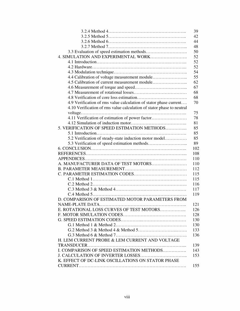
TABLE OF CONTENTS PLAGIARISM………………………………………………………………... iii ABSTRACT…………………………………………………………………... iv ÖZ………………………………………………………………………..…… v ACKNOWLEDGEMENT………………………………………………..…... vi TABLE OF CONTENTS…………………………………………………….. vii LIST OF TABLES……………………………………………………………. ix LIST OF FIGURES…………………………………………………………... xi CHAPTER 1 INTRODUCTION………………………………………………….…. 1 1.1 Introduction………………………………………………..…... 1 1.2 Contents of thesis……………………………………………… 2 2. PREDICTION OF INDUCTION MOTOR PARAMETERS FROM

MANUFACTURER DATA……………………………………………... 4 2.1 Introduction……………………………………………………. 4 2.2 Method 1………………………………………………………. 6 2.2.1 Calculation of Rr…………………………………….. 8 2.2.2 Calculation of Rc…………………………………….. 9 2.2.3 Calculation of Xm…………………………………… 9 2.2.4 Calculation of Xs…………………………………….. 9 2.3 Method 2………………………………………………………. 10 2.3.1 Calculation of Rc & Xm……………………………... 12 2.3.2 Calculation of Rr & Xs………………………………. 12 2.4 Method 3………………………………………………………. 13 2.4.1 Calculation of Rr…………………………………….. 14 2.4.2 Calculation of Rc & Xm……………………………... 15 2.4.3 Calculation of Xs…………………………………….. 15 2.5 Method 4………………………………………………………. 17 2.6 Method 5…………..…………………………………………... 18 2.6.1 Calculation of Xm……………..…………………….. 18 2.6.2 Calculation of Xs…………………………………….. 18 2.6.3 Calculation of Rr…………………………………….. 20 2.6.4 Calculation of Rc…………………………………….. 20 2.7 Results…………………………………………………………. 21 3. PREDICTION OF MOTOR SPEED…………………………………. 30 3.1 Introduction……………………………………………………. 30 3.2 Investigation of speed estimation methods……………………. 32 3.2.1 Method 1…………………………………………….. 32 3.2.2 Method 2…………………………………………….. 35 3.2.3 Method 3…………………………………………….. 37

viii

3.2.4 Method 4…………………………………………….. 39 3.2.5 Method 5…………………………………………….. 42 3.2.6 Method 6…………………………………………….. 44 3.2.7 Method 7……………………………………………... 48 3.3 Evaluation of speed estimation methods………………………. 50 4. SIMULATION AND EXPERIMENTAL WORK……………………. 52 4.1 Introduction…………………………………………..………... 52 4.2 Hardware………………………………………..……………... 52 4.3 Modulation technique………………………………………….. 54 4.4 Calibration of voltage measurement module…………………... 55 4.5 Calibration of current measurement module…………………... 62 4.6 Measurement of torque and speed……………………………... 67 4.7 Measurement of rotational losses……………………………… 68 4.8 Verification of core loss estimation……………………………. 68 4.9 Verification of rms value calculation of stator phase current…. 70 4.10 Verification of rms value calculation of stator phase to neutral

voltage……………………………………………………………... 75 4.11 Verification of estimation of power factor…………………… 78 4.12 Simulation of induction motor……………………………….. 81 5. VERIFICATION OF SPEED ESTIMATION METHODS…………... 85 5.1 Introduction……………………………………………………. 85 5.2 Verification of steady-state induction motor model…………… 85 5.3 Verification of speed estimation methods……………………... 89 6. CONCLUSION……………………………………………………….. 102 REFERENCES…………………………………………………………... 108 APPENDICES…………………………………………………………… 110 A. MANUFACTURER DATA OF TEST MOTORS…………………… 110 B. PARAMETER MEASUREMENT…………………………………… 112 C. PARAMETER ESTIMATION CODES……………………………… 115 C.1 Method 1………………………………………………………. 115 C.2 Method 2………………………………………………………. 116 C.3 Method 3 & Method 4………………………………………… 117 C.4 Method 5………………………………………………………. 119 D. COMPARISON OF ESTIMATED MOTOR PARAMETERS FROM

NAME-PLATE DATA………………………………………………….. 121 E. ROTATIONAL LOSS CURVES OF TEST MOTORS……………... 126 F. MOTOR SIMULATION CODES……………………………………. 128 G. SPEED ESTIMATION CODES…………...………………………… 130 G.1 Method 1 & Method 2…………...……………………………. 130 G.2 Method 3 & Method 4 & Method 5……………………...……. 133 G.3 Method 6 & Method 7………………………………...………. 136 H. LEM CURRENT PROBE & LEM CURRENT AND VOLTAGE

TRANSDUCER……………………………………………..…………... 139 I. COMPARISON OF SPEED ESTIMATION METHODS……………. 143 J. CALCULATION OF INVERTER LOSSES………………………….. 153 K. EFFECT OF DC-LINK OSCILLATIONS ON STATOR PHASE

CURRENT………………………………………………………………. 155

ix

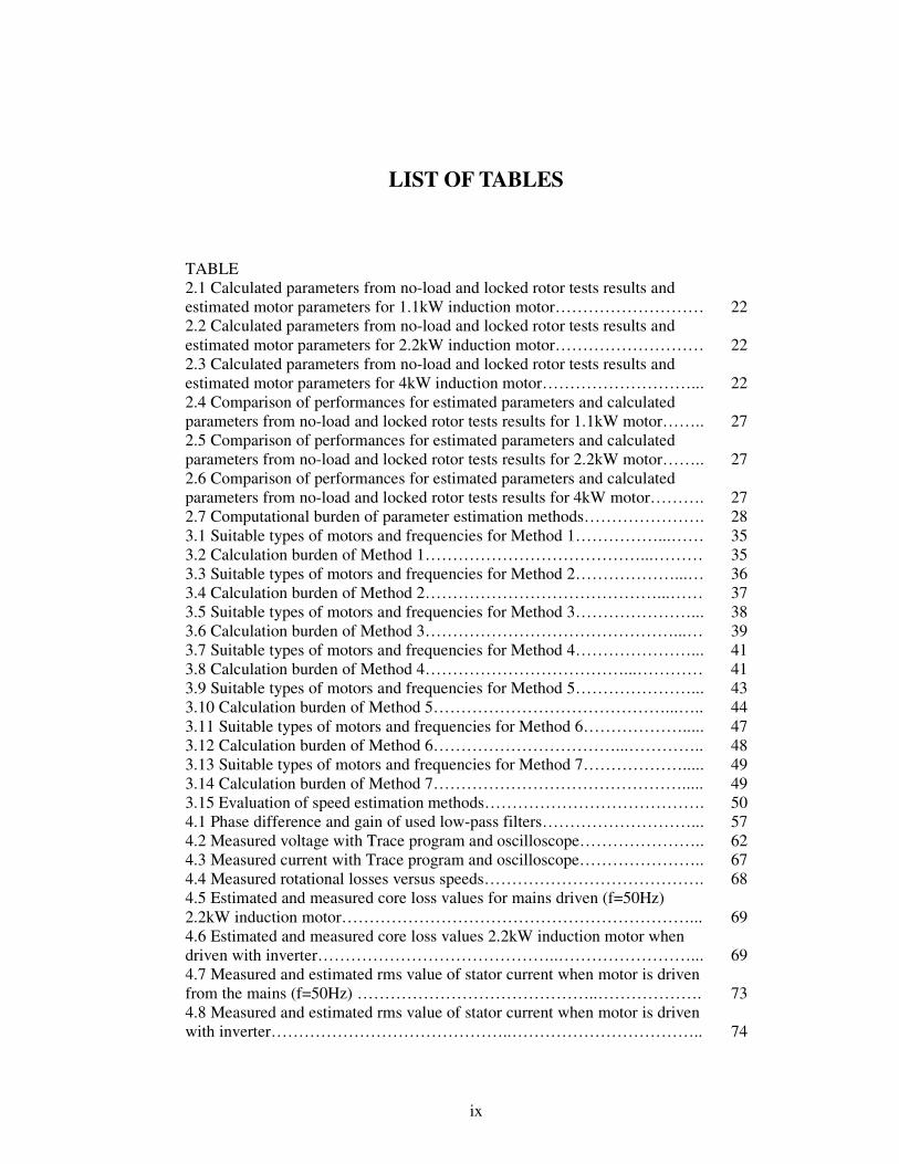
LIST OF TABLES TABLE 2.1 Calculated parameters from no-load and locked rotor tests results and estimated motor parameters for 1.1kW induction motor……………………… 22 2.2 Calculated parameters from no-load and locked rotor tests results and estimated motor parameters for 2.2kW induction motor……………………… 22 2.3 Calculated parameters from no-load and locked rotor tests results and estimated motor parameters for 4kW induction motor………………………... 22 2.4 Comparison of performances for estimated parameters and calculated parameters from no-load and locked rotor tests results for 1.1kW motor…….. 27 2.5 Comparison of performances for estimated parameters and calculated parameters from no-load and locked rotor tests results for 2.2kW motor…….. 27 2.6 Comparison of performances for estimated parameters and calculated parameters from no-load and locked rotor tests results for 4kW motor………. 27 2.7 Computational burden of parameter estimation methods…………………. 28 3.1 Suitable types of motors and frequencies for Method 1……………...…… 35 3.2 Calculation burden of Method 1…………………………………...……… 35 3.3 Suitable types of motors and frequencies for Method 2………………...… 36 3.4 Calculation burden of Method 2……………………………………...…… 37 3.5 Suitable types of motors and frequencies for Method 3…………………... 38 3.6 Calculation burden of Method 3………………………………………...… 39 3.7 Suitable types of motors and frequencies for Method 4…………………... 41 3.8 Calculation burden of Method 4………………………………...………… 41 3.9 Suitable types of motors and frequencies for Method 5…………………... 43 3.10 Calculation burden of Method 5……………………………………...….. 44 3.11 Suitable types of motors and frequencies for Method 6………………..... 47 3.12 Calculation burden of Method 6……………………………...………….. 48 3.13 Suitable types of motors and frequencies for Method 7………………..... 49 3.14 Calculation burden of Method 7………………………………………..... 49 3.15 Evaluation of speed estimation methods…………………………………. 50 4.1 Phase difference and gain of used low-pass filters………………………... 57 4.2 Measured voltage with Trace program and oscilloscope………………….. 62 4.3 Measured current with Trace program and oscilloscope………………….. 67 4.4 Measured rotational losses versus speeds…………………………………. 68 4.5 Estimated and measured core loss values for mains driven (f=50Hz) 2.2kW induction motor………………………………………………………... 69 4.6 Estimated and measured core loss values 2.2kW induction motor when driven with inverter……………………………………..……………………... 69 4.7 Measured and estimated rms value of stator current when motor is driven from the mains (f=50Hz) ……………………………………..………………. 73 4.8 Measured and estimated rms value of stator current when motor is driven with inverter……………………………………..…………………………….. 74

x

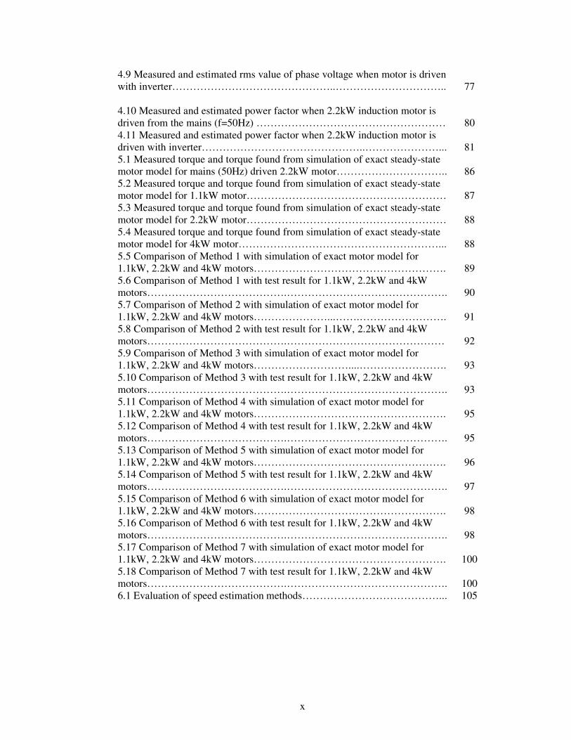
4.9 Measured and estimated rms value of phase voltage when motor is driven with inverter………………………………………..………………………….. 77 4.10 Measured and estimated power factor when 2.2kW induction motor is driven from the mains (f=50Hz) ……………………………………………… 80 4.11 Measured and estimated power factor when 2.2kW induction motor is driven with inverter………………………………………..…………………... 81 5.1 Measured torque and torque found from simulation of exact steady-state motor model for mains (50Hz) driven 2.2kW motor………………………….. 86 5.2 Measured torque and torque found from simulation of exact steady-state motor model for 1.1kW motor………………………………………………… 87 5.3 Measured torque and torque found from simulation of exact steady-state motor model for 2.2kW motor………………………………………………… 88 5.4 Measured torque and torque found from simulation of exact steady-state motor model for 4kW motor…………………………………………………... 88 5.5 Comparison of Method 1 with simulation of exact motor model for 1.1kW, 2.2kW and 4kW motors………………………………………………. 89 5.6 Comparison of Method 1 with test result for 1.1kW, 2.2kW and 4kW motors………………………………….………………………………………. 90 5.7 Comparison of Method 2 with simulation of exact motor model for 1.1kW, 2.2kW and 4kW motors…………………...…….……………………. 91 5.8 Comparison of Method 2 with test result for 1.1kW, 2.2kW and 4kW motors………………………………….……………………………………… 92 5.9 Comparison of Method 3 with simulation of exact motor model for 1.1kW, 2.2kW and 4kW motors………………………....……………………. 93 5.10 Comparison of Method 3 with test result for 1.1kW, 2.2kW and 4kW motors………………………………….………………………………………. 93 5.11 Comparison of Method 4 with simulation of exact motor model for 1.1kW, 2.2kW and 4kW motors………………………………………………. 95 5.12 Comparison of Method 4 with test result for 1.1kW, 2.2kW and 4kW motors………………………………….………………………………………. 95 5.13 Comparison of Method 5 with simulation of exact motor model for 1.1kW, 2.2kW and 4kW motors………………………………………………. 96 5.14 Comparison of Method 5 with test result for 1.1kW, 2.2kW and 4kW motors………………………………….………………………………………. 97 5.15 Comparison of Method 6 with simulation of exact motor model for 1.1kW, 2.2kW and 4kW motors………………………………………………. 98 5.16 Comparison of Method 6 with test result for 1.1kW, 2.2kW and 4kW motors………………………………….………………………………………. 98 5.17 Comparison of Method 7 with simulation of exact motor model for 1.1kW, 2.2kW and 4kW motors………………………………………………. 100 5.18 Comparison of Method 7 with test result for 1.1kW, 2.2kW and 4kW motors………………………………….………………………………………. 100 6.1 Evaluation of speed estimation methods…………………………………... 105

xi

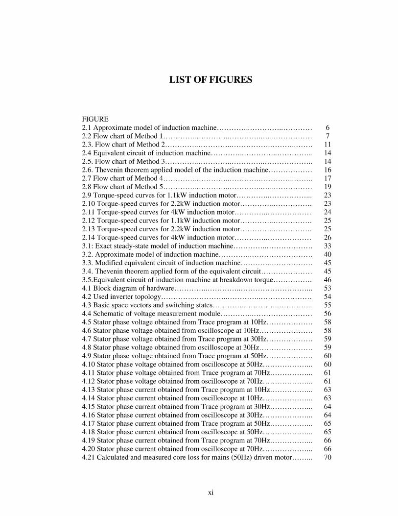
LIST OF FIGURES FIGURE 2.1 Approximate model of induction machine…………..…………..………… 6 2.2 Flow chart of Method 1…………..…………..…………..…...…………… 7 2.3. Flow chart of Method 2…………..…………..…………….………..……. 11 2.4 Equivalent circuit of induction machine…………..…………..…………... 14 2.5. Flow chart of Method 3…………..…………..…………..……………….. 14 2.6. Thevenin theorem applied model of the induction machine……………… 16 2.7 Flow chart of Method 4…………..…………..………….…………..…….. 17 2.8 Flow chart of Method 5…………..…………..…………..…...…………… 19 2.9 Torque-speed curves for 1.1kW induction motor…………..……………... 23 2.10 Torque-speed curves for 2.2kW induction motor…………..……………. 23 2.11 Torque-speed curves for 4kW induction motor…………..……………… 24 2.12 Torque-speed curves for 1.1kW induction motor…………..……………. 25 2.13 Torque-speed curves for 2.2kW induction motor…………..……………. 25 2.14 Torque-speed curves for 4kW induction motor…………..……………… 26 3.1: Exact steady-state model of induction machine…………..………………. 33 3.2. Approximate model of induction machine…………..……………………. 40 3.3. Modified equivalent circuit of induction machine…………..……………. 45 3.4. Thevenin theorem applied form of the equivalent circuit………………… 45 3.5.Equivalent circuit of induction machine at breakdown torque……………. 46 4.1 Block diagram of hardware…………..…………..………………………... 53 4.2 Used inverter topology…………..…………..…………..………………… 54 4.3 Basic space vectors and switching states…………..…………..………….. 55 4.4 Schematic of voltage measurement module…………..…………………… 56 4.5 Stator phase voltage obtained from Trace program at 10Hz………………. 58 4.6 Stator phase voltage obtained from oscilloscope at 10Hz…………………. 58 4.7 Stator phase voltage obtained from Trace program at 30Hz………………. 59 4.8 Stator phase voltage obtained from oscilloscope at 30Hz…………………. 59 4.9 Stator phase voltage obtained from Trace program at 50Hz………………. 60 4.10 Stator phase voltage obtained from oscilloscope at 50Hz………………... 60 4.11 Stator phase voltage obtained from Trace program at 70Hz……………... 61 4.12 Stator phase voltage obtained from oscilloscope at 70Hz………………... 61 4.13 Stator phase current obtained from Trace program at 10Hz……………... 63 4.14 Stator phase current obtained from oscilloscope at 10Hz………………... 63 4.15 Stator phase current obtained from Trace program at 30Hz……………... 64 4.16 Stator phase current obtained from oscilloscope at 30Hz………………... 64 4.17 Stator phase current obtained from Trace program at 50Hz……………... 65 4.18 Stator phase current obtained from oscilloscope at 50Hz………………... 65 4.19 Stator phase current obtained from Trace program at 70Hz……………... 66 4.20 Stator phase current obtained from oscilloscope at 70Hz………………... 66 4.21 Calculated and measured core loss for mains (50Hz) driven motor……... 70

xii

4.22 Measured stator currents at 30 Hz………………………………………... 71 4.23 Measured stator currents at 70 Hz………………………………………... 71 4.24 Measured and estimated rms value of stator current when motor is driven from the mains (f=50Hz) ……………………………………………………… 73 4.25 Measured and estimated rms value of stator current when motor is driven at 30Hz with inverter…………………………………………………………... 74 4.26 Measured phase to neutral voltages at 30Hz……………………………... 76 4.27 Measured phase to neutral voltages at 70Hz……………………………... 76 4.28 Measured and estimated rms value of phase voltage when motor is driven at 30Hz with inverter…………………………………………………... 77 4.29 Magnetic axes of the motor………………………………………………. 78 4.30 Flow chart of simulation model………………………………………….. 82 4.31 Linear portion of torque-speed curves for experiment result and simulation of 2.2 kW motor…………………………………………………… 83 4.32 Torque-speed curves prepared with simulation for 10, 30, 50 and 70Hz... 83 6.1 Measurement module for rms value of current……………………………. 106

1

CHAPTER 1

INTRODUCTION

1.1. Introduction

Prior to 1950s nearly all industrial applications required the use of a DC motor

drive since AC motors were not suitable for speed control with the technology

available at the time [1]. Nowadays modern AC motor drive performance is

comparable with DC motor drive. This goal has been achieved because development in

power electronics and microprocessors led to introduction of sophisticated AC motor

drives [2].

Number of AC motor drives using induction motor is still increasing in

industrial applications. Majority are based on scalar control principle where the control

algorithm can be implemented on simple microcontrollers. Sophisticated control

methods require fast processors which increase the price of drives [2].

Cost saving aspects are important for applications at low power drives below 5

kW. At high power, the power components dominate the system cost. Therefore fast

processor can be used at high power drives [7,8].

To reduce the initial cost of the low cost motor drives, it is necessary to use low

performance microprocessors. Since price of the microprocessor is proportional to the

performance of the microprocessor, in low cost drives it is necesary to control speed ad

torque with minimum number of calculations and minimum measurements.

The aim of this study is achieving speed estimation accuracy and torque

estimation accuracy with minimum number of calculations and measurements.

Any method for speed prediction is based on a model of the motor and the

drive. The best accuracy of prediction for an induction motor may be expected when

2

the exact model is used. However, this would bring too much computational burden

and would require knowledge of all the motor parameters.

Motor parameters can be calculated from no-load and locked rotor tests or can

be estimated. On-line estimation of parameters places an important burden of the

microprocessor. Therefore, low cost drives avoid this approach and often estimate

parameters from the user supplied motor label data. Some new methods are proposed

in this study to estimate motor parameters off-line from manufacturer’s data.

Since accurate knowledge of the motor parameters is required to predict speed

from exact motor model, one of the aims of this study is achieving speed or torque

estimation accuracy with minimum number of the motor parameters.

Various speed estimation techniques are described in literature. The most

common method used in practice is linearization of torque-speed curve [5,10]. Base

frequency, speed, output power, number of poles and stator resistance are used in this

method. These data are obtained at base frequency and rated torque. This method has

drawbacks at high loads and in the field weakening region.

Another speed estimation method, which does not require motor parameters

except stator resistance, is based on a non-linear relationship between air-gap power

and slip speed [6]. Base frequency, voltage, current, speed, power factor, output power,

number of poles, efficiency, breakdown torque at base frequency and stator resistance

are used in this method. These data are obtained at base frequency and rated torque. In

this method, since the breakdown torque is assumed to be constant and stator resistance

is neglected at calculation of slip speed, this approach is not suitable for high speeds

and small motors, at which voltage drop on the stator resistance is comparable to input

voltage at low frequencies. So there is room for improvement.

1.2 Contents of the thesis

Chapter 2 includes a brief explanation of proposed parameter estimation

methods. In this chapter, results of parameter estimation methods are also investigated.

Chapter 3 is assigned to investigate the some of the speed estimation methods

found in literature and proposed methods. A theoretical evaluation of these methods is

also given in this chapter.

3

Chapter 4 is assigned for simulation and experimental work. In this chapter,

hardware and modulation technique of the drive used for tests are briefly explained.

Then calibration of voltage and current measurement modules are explained. Then

measurement of torque, speed and rotational losses are explained. Then estimation of

core loss, estimation of power factor, calculation of rms value of current and voltage

are verified. Finally simulation software used in this thesis is based on exact induction

motor model is explained.

Chapter 5 is assigned to verification of the exact induction motor model and

evaluation of accuracy of speed estimation methods presented in the previous chapters.

Chapter 6 includes the conclusion of this study.

4

CHAPTER 2

PREDICTION OF INDUCTION MOTOR PARAMETERS

FROM MANUFACTURER DATA

2.1 Introduction

The majority of variable speed drives are used in general purpose applications.

In such applications, the most important factors are ease of initialization and low

overall cost.

Motor parameters and motor ratings must be known to initialize the drive.

Using these data, the drive often predicts the motor speed and some control is applied,

if the user prefers to operate the drive in speed control mode or torque control mode.

Classical method for parameter determination uses the no-load and locked rotor tests

results. This classical parameter determination method is sometimes impractical for

initializing a motor drive. To simplify the initialization process, motor parameters can

be estimated from manufacturer data by the drive processor. When literature (Science

Citation Index 1945-2004 and IEEE archieves) is investigated, only three research

methods are found on this issue.

In one of these methods, motor parameters are estimated from manufacturer

data with a numerical method [17]. This off-line parameter estimation method requires

a computer and necessary software to make these calculations. In this method, initial

values of motor parameters are calculated with some assumptions. Then, each

parameter is changed from initial value to zero with small steps. This step size defines

the accuracy. For each possible combination of parameters, exact equivalent circuit of

induction machine is used and mechanical power, reactive power at full load and

5

breakdown torque are calculated. Results of these calculations are compared with

manufacturer supplied data and errors of these calculations are found. Then each error

is weighted in accordance to the importance of these calculations by the user of this

method. Total weight of the errors is calculated for each possible combination. This

method is finalized by selecting the motor parameters by looking into minimum error

weight. It is reported that this method is applied to 223 motors and error of this method

is nearly 1%.

In [26], motor parameters are estimated from manufacturer data such as name-

plate data and motor performance characteristics. This method is based on a non-linear

optimization routine. Therefore this method is not suitable to be embedded on a low

performance microprocessor.

In [27], parameter estimation method requires the name-plate data, ratio of

starting to full load torque and the efficiency and power factor values at half and full

load. Since motor data at half load are not accessible in manufacturer data, this method

is not suitable for the aim of this study.

Since these methods are not suitable to be embedded on a low performance

microprocessor, it is decided to propose a method which has good accuracy with lower

computational burden.

In this chapter, several methods are proposed for prediction of motor

parameters from manufacturer supplied data or motor label. These methods are

examined on 1.1 kW, 2.2 kW and 4 kW induction motors. To verify the proposed

methods, no-load and locked rotor tests are applied to these motors. Motor parameters

are calculated from no-load and locked rotor tests results and compared with estimated

motor parameters.

Predicted torque-speed characteristics of the test motors are also compared with

measurements at 50Hz. Since the drive is normally operated in the portion of torque-

speed curve between no-load speed and full-load speed, the predictions are done for

this portion of the torque-speed curve.

It is seen in tests that some of the manufacturer supplied data may be different

from test results. Parameter predictions are made using manufacturer’s data and

presented in Appendix A. However, all of the parameter predictions in this section are

done on the basis of motor label data determined from tests on the three test motors.

6

The predicted performance for the proposed parameter identification method

(torque, power factor, stator current) are compared with the predicted performance of

the motors from no-load and locked rotor parameters and measured performance of the

motors.

In the following sections, each of the proposed methods is described.

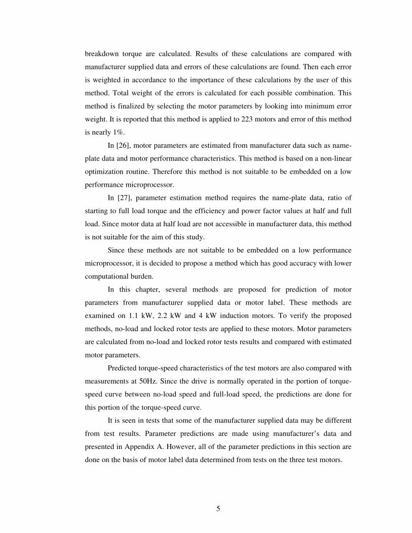
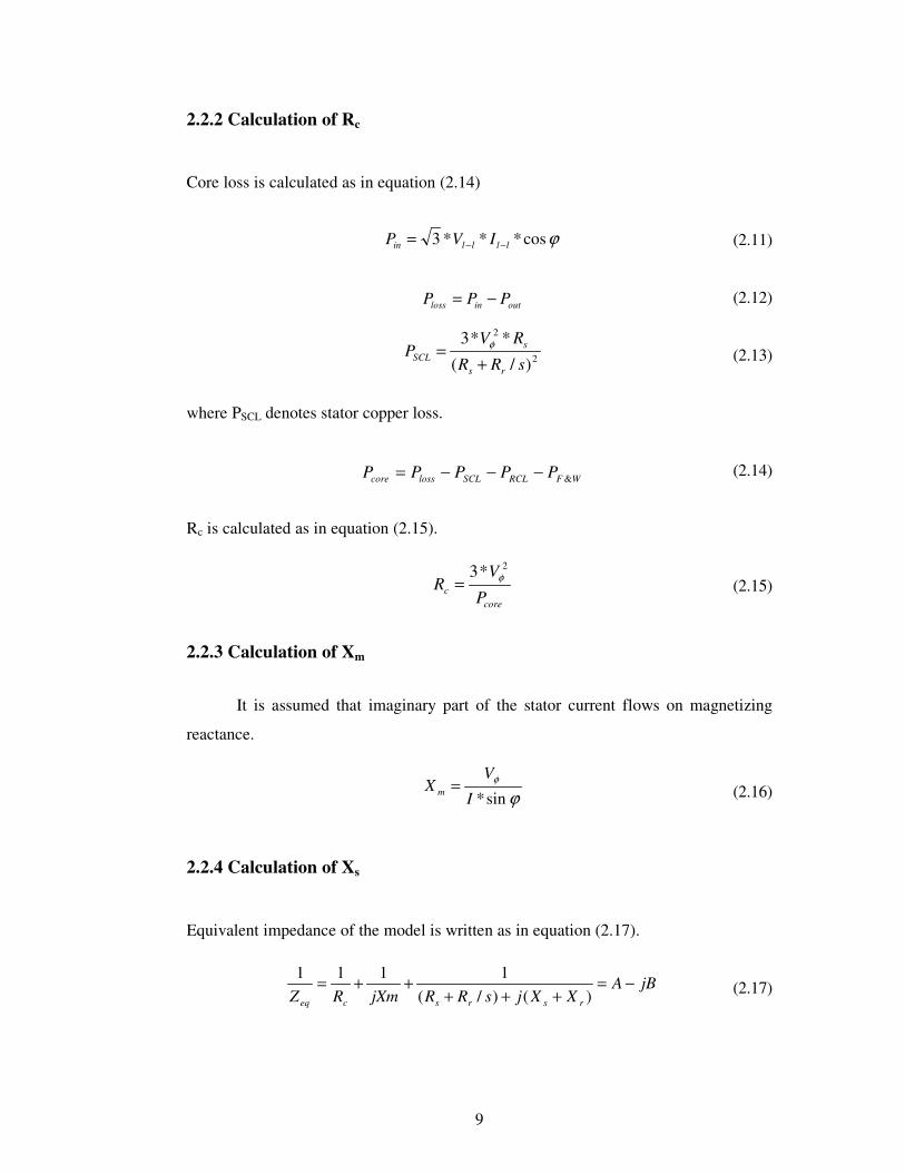
2.2 Method 1

In this method, approximate circuit model, which is seen in Fig.2.1, is used.

Rated voltage, rated current, rated power factor, output power, frequency, rotor speed

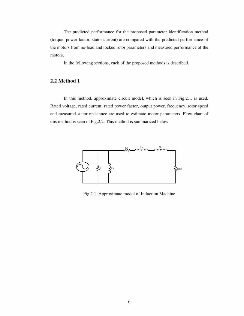
and measured stator resistance are used to estimate motor parameters. Flow chart of

this method is seen in Fig.2.2. This method is summarized below.

X sR s

R c X m

X r

R r/s

Fig.2.1. Approximate model of Induction Machine

7

WFRCLAGout PPPP &−−=

rrr

rWFOUT RIs

RIPP **3**3)( 22

& −=+

)1

(***3)( 2& s

sRIPP rrWFOUT

−=+

outWF PP *01.0& =

C A L C U L A T E R E F E R R E DR O T O R R E S I S T A N C E

C A L C U L A T E C O R E L O S S

C A L C U L A T E R c

C A L C U L A T EM A G N E T I Z I N G

R E A C T A N C E

W R I T E E Q U I V A L E N TI M P E D A N C E A N D

C A L C U L A T E S T A T O RL E A K A G E R E A C T A N C E

C A L C U L A T E S T A T O RC O P P E R L O S S

I N P U T : P o u t , V , I , s , R s ,P O W E R F A C T O R

C A L C U L A T E R O T O RC O P P E R L O S S E S

Fig.2.2 Flow chart of Method 1

It is assumed that friction and windage losses are equal to the 1% of output

power. Another assumption is that stator leakage reactance is neglected for the

calculation of magnetizing reactance. That imaginary part of stator current flows on the

magnetizing reactance is assumed. Rotor copper losses can be calculated as in equation

(2.5).

(2.1)

(2.2)

(2.3)

(2.4)

8

)1

(*)(**3 &2

ss

PPRIP WFOUTrrRCL −+==

22 )()/( rsrS

rXXsRR

VI

+++= φ

rs XX = )*4()/( 22srs XsRR >>+

2

2

)/(

**3

sRR

RVP

rs

rRCL +

= φ

0**)*3**2

(*)( 2222 =+−+ RCLsr

RCLsr

RCL PRRVs

PRR

sP

φ

2

22

)/( sRR

VI

rsr +

= φ

(2.5)

where PAG denotes air-gap power, PF&W denotes friction and windage losses, PRCL

denotes rotor copper loss, Pout denotes output power, s denotes slip, Ir denotes referred

rotor current and Rr denotes referred rotor resistance.

2.2.1 Calculation of Rr

Referred rotor current can be written as

(2.6)

where φV denotes phase voltage.

Assume that

& (2.7)

If the assumptions seen above are valid, rotor current and rotor copper losses formulas

can be rearranged as below

(2.8)

(2.9)

from equation (2.9)

(2.10)

in equation (2.10), only referred rotor resistance is unknown, so rotor resistance is

found by calculating the roots of equation (2.10).

9

ϕcos***3 llllin IVP −−=

outinloss PPP −=

2

2

)/(

**3

sRR

RVP

rs

sSCL +

= φ

ϕφ

sin*I

VX m =

jBAXXjsRRjXmRZ rsrsceq

−=+++

++=)()/(

1111

WFRCLSCLlosscore PPPPP &−−−=

corec P

VR

2*3 φ=

2.2.2 Calculation of Rc

Core loss is calculated as in equation (2.14)

(2.11)

(2.12)

(2.13)

where PSCL denotes stator copper loss.

(2.14)

Rc is calculated as in equation (2.15).

(2.15)

2.2.3 Calculation of Xm

It is assumed that imaginary part of the stator current flows on magnetizing

reactance.

(2.16)

2.2.4 Calculation of Xs

Equivalent impedance of the model is written as in equation (2.17).

(2.17)

10

AB−=− )tan( ϕ

22 *4)/(*2)/(*tantan1

srs

srs

cm XsRRXsRR

RX ++−+=− ϕϕ

0)/(*tan)/(*tan1

*2*tan1

*4 22 =+−+���

����

�−++��

�

����

�− sRRsRR

RXXX

RX rsrscm

sscm

ϕϕϕ

If tangent of load angle is written as in equation (2.18) and substituting the

equalities of A and B, equation (2.20) is achieved.

(2.18)

(2.19)

(2.20)

Only stator leakage reactance is unknown in equation (2.20), so stator leakage

reactance can be calculated by solving the roots of equation (2.20).

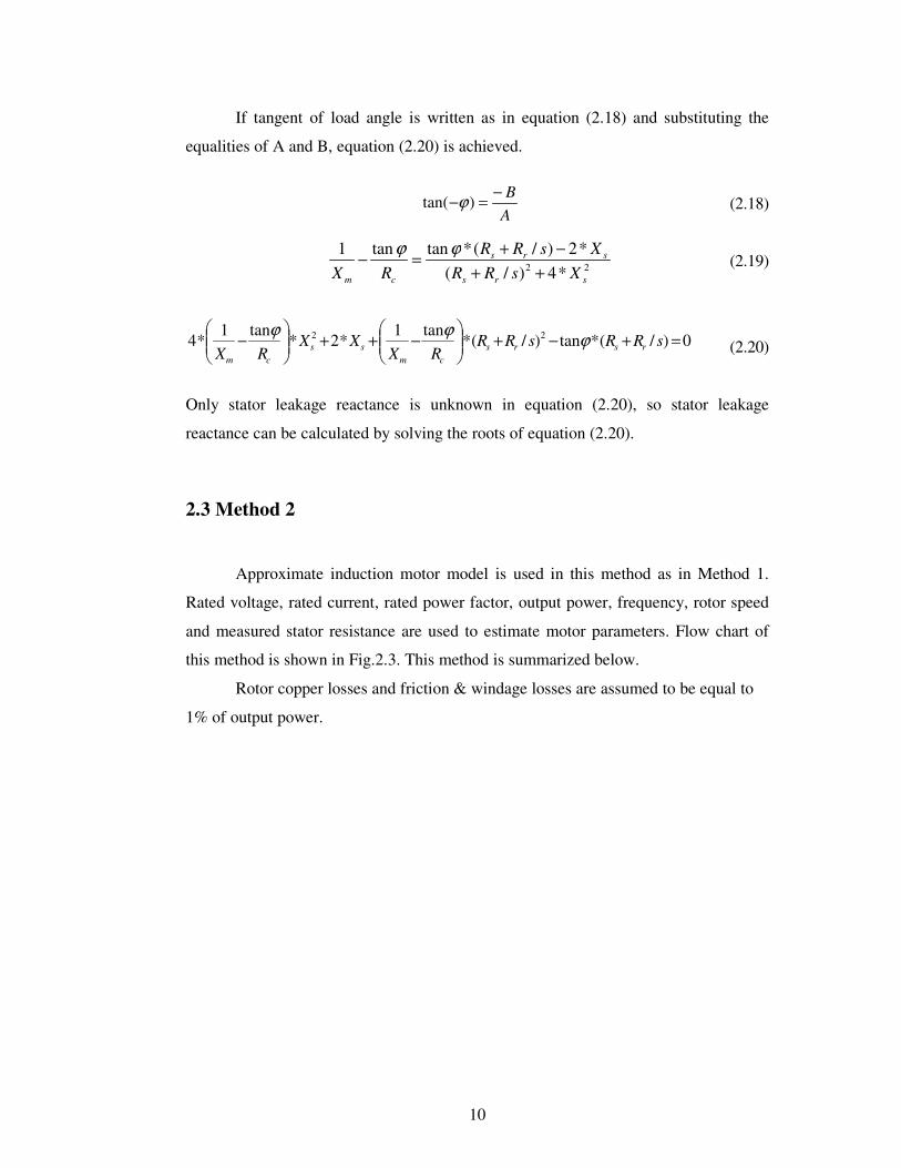
2.3 Method 2

Approximate induction motor model is used in this method as in Method 1.

Rated voltage, rated current, rated power factor, output power, frequency, rotor speed

and measured stator resistance are used to estimate motor parameters. Flow chart of

this method is shown in Fig.2.3. This method is summarized below.

Rotor copper losses and friction & windage losses are assumed to be equal to

1% of output power.

11

F IN D R O T O R C O P P E RL O S S E S

C A L C U L A T E C O R EL O S S B Y U S IN G E X A C TS T A T O R C O P P E R L O S S

F IN D R c

F IN D X m

W R IT E R O T O R C O P P E RL O S S B Y U S IN G

T H E V E N IN T H E O R E M ,A N D F IN D X s A S A

F U N C T IO N O F R r

W R IT E E Q U IV A L E N TIM P E D A N C E

W R IT E T A N G E N T O FP O W E R F A C T O RA N G L E B Y U S IN G

E Q U IV A L E N TIM P E D A N C E

IN S E R T E Q U A L IT Y O FX s W H IC H IS F O U N D

IN T H E A B O V EE Q U A T IO N . (N O W

O N L Y R r ISU N K N O W N )

F IN D R r A N D T H E N X s

IN P U T D A T A

Fig.2.3. Flow chart of Method 2

12

22 )()/( rsrS

rXXsRR

VI

+++= φ

rrRCL RIP **3 2=

22

2 )/(**3

*4 sRRP

RVX rs

RCL

rs +−= φ

ssSCL RIP **3 2=

corec P

VR

2*3 φ=

ϕφ

sin*I

VX m =

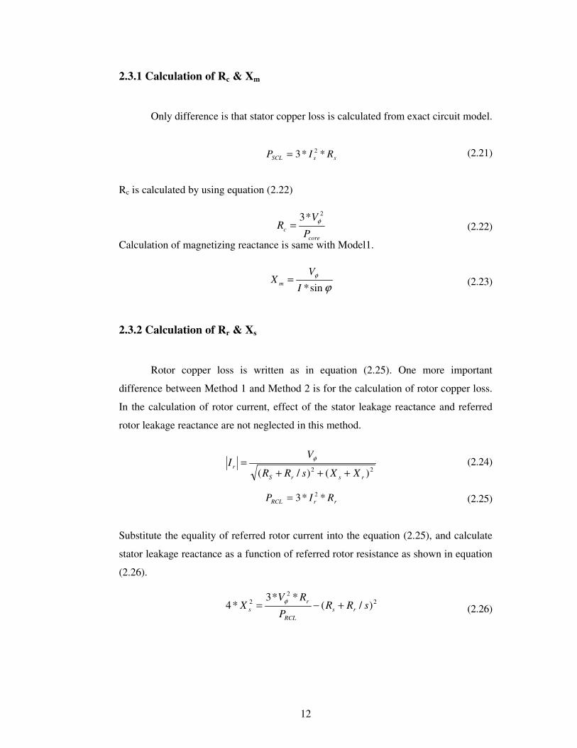
2.3.1 Calculation of Rc & Xm

Only difference is that stator copper loss is calculated from exact circuit model.

(2.21)

Rc is calculated by using equation (2.22)

(2.22)

Calculation of magnetizing reactance is same with Model1.

(2.23)

2.3.2 Calculation of Rr & Xs

Rotor copper loss is written as in equation (2.25). One more important

difference between Method 1 and Method 2 is for the calculation of rotor copper loss.

In the calculation of rotor current, effect of the stator leakage reactance and referred

rotor leakage reactance are not neglected in this method.

(2.24)

(2.25)

Substitute the equality of referred rotor current into the equation (2.25), and calculate

stator leakage reactance as a function of referred rotor resistance as shown in equation

(2.26).

(2.26)

13

22 *4)/(*2)/(*tantan1

srs

srs

cm XsRRXsRR

RX ++−+=− ϕϕ

[ ]22 *4)/(1tan

)/(*tan*2 srsmc

rss XsRRXR

sRRX ++���

����

�−++= ϕϕ

��

�

�

��

�

����

����

�−++=

RCL

r

mcrss P

RV

XRsRRX

**31tan)/(*tan*2

2φϕϕ

22

22 **31tan

)/(*tan)/(**3

���

�

�

��

�

�

��

�

����

����

�−++=+−

RCL

r

mcrsrs

RCL

r

P

RV

XRsRRsRR

P

RV φφ ϕϕ

If equivalent impedance and tan (�) are written, stator leakage reactance is found as a

function of referred rotor resistance.

(2.27)

(2.28)

Substitute the equality of Xs2 which is found equation (2.26) into the equation (2.28)

(2.29)

If square of equation (2.29) is calculated and equality of 24 sX is substituted into

equation (2.26), equation (2.30), which is independent from stator leakage reactance, is

achieved.

(2.30)

In equation (2.30), only referred rotor resistance is unknown. Referred rotor

resistance is found by calculating the roots of equation (2.30). Stator leakage reactance

is calculated by substituting calculated referred rotor resistance into equation (2.29).

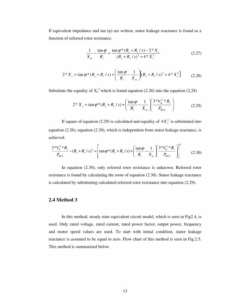
2.4 Method 3

In this method, steady state equivalent circuit model, which is seen in Fig2.4, is

used. Only rated voltage, rated current, rated power factor, output power, frequency

and motor speed values are used. To start with initial condition, stator leakage

reactance is assumed to be equal to zero. Flow chart of this method is seen in Fig.2.5.

This method is summarized below.

14

X sR s

R c X m

X r

R r / s

E m

Fig.2.4 Equivalent circuit of induction machine

A S S U M E X s = 0

U S I N G R O T O R C O P P E RL O S S , C A L C U L A T E R r

C A L C U L A T E X m

C A L C U L A T E C O R EL O S S , A N D T H E N

C A L C U L A T E R c

W R I T E E Q U A L I T Y O FA I R G A P P O W E R B Y

U S I N G T H E V E N I NE Q U I V A L E N T C I R C U I T

( O N L Y X s I SU N K N O W N )

C A L C U L A T E X s

C A L C U L A T E E m

I N P U T D A T A

Fig.2.5. Flow chart of Method 3

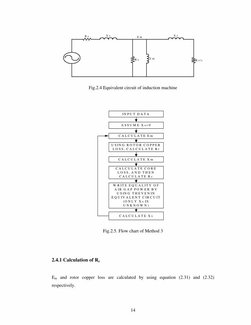
2.4.1 Calculation of Rr

Em and rotor copper loss are calculated by using equation (2.31) and (2.32)

respectively.

15

sssm IjXRVE *)( +−= φ

0***3* 22

22 =+− rRCLrr

RCL XPRERs

P

ϕsin*IE

X mm =

ssSCL RIP **3 2=

WFRCLSCLlosscore PPPPP &−−−=

( )22

2

)/(**3

rr

rmRCL XsR

REP

+=

core

m

c P

ER

2

*3=

(2.31)

(2.32)

If equation (2.32) is rearranged, equation (2.33) is achieved.

(2.33)

Rotor copper loss is calculated by using equation (2.5). Only referred rotor

resistance is unknown in equation (2.33). Referred rotor resistance is calculated by

solving equation (2.33).

2.4.2 Calculation of Rc & Xm

It is assumed that imaginary part of stator current flows on magnetizing

reactance. Magnetizing reactance is calculated by using equation (2.34).

(2.34)

Core loss and Rc are calculated by using equation (2.36) and (2.37) respectively.

(2.35)

(2.36)

(2.37)

2.4.3 Calculation of Xs

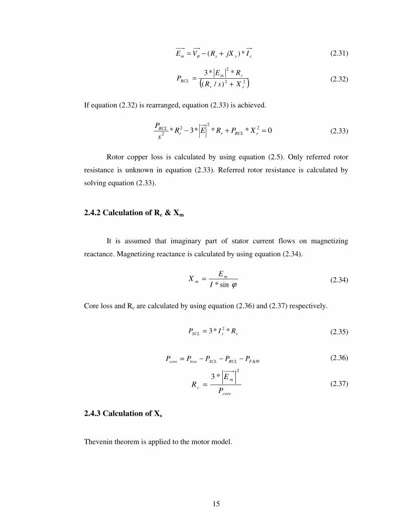
Thevenin theorem is applied to the motor model.

16

ms

mTH XX

XVV

+= *φ

sTH XX =

2

* ���

����

�

+=

ms

msTH XX

XRR

22 )()/( rTHrTH

THr

XXsRR

VI

+++=

WFRCLoutAG PPPP &++=

��

�

�+++

++

=22

2

22

22

)()/)(

*()(

)/(***3

rsrms

msms

rmAG

XXsRXX

XRXX

sRXVP φ

V th

X t hR t h X r

R r / s

Fig.2.6. Thevenin theorem applied model of the induction machine

(2.38)

(2.39)

(2.40)

(2.41)

Air gap power is calculated by using equation (2.42).

(2.42)

(2.43)

Only stator leakage reactance is unknown in equation (2.43). Stator leakage

reactance is calculated by calculating the roots of equation (2.43). To finalize the

parameter estimation, any stop criteria is not used. Process explained above is iterated

3 times with new values.

17

2.5 Method 4

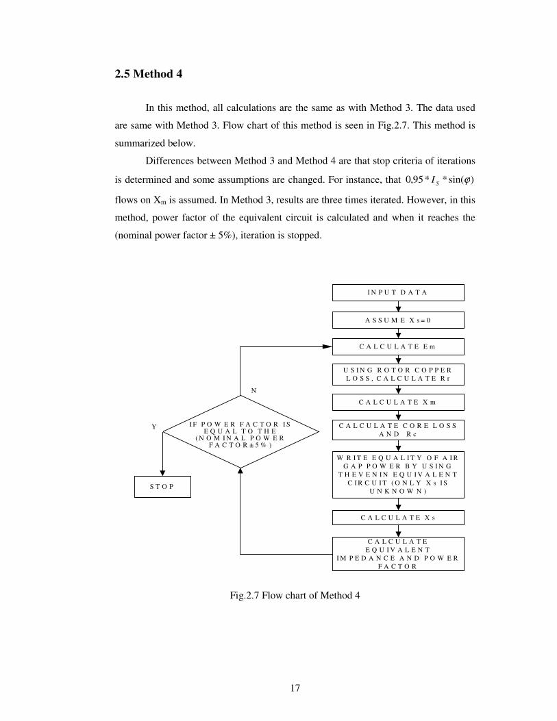
In this method, all calculations are the same as with Method 3. The data used

are same with Method 3. Flow chart of this method is seen in Fig.2.7. This method is

summarized below.

Differences between Method 3 and Method 4 are that stop criteria of iterations

is determined and some assumptions are changed. For instance, that )sin(**95,0 ϕSI

flows on Xm is assumed. In Method 3, results are three times iterated. However, in this

method, power factor of the equivalent circuit is calculated and when it reaches the

(nominal power factor ± 5%), iteration is stopped.

A S S U M E X s = 0

U S I N G R O T O R C O P P E RL O S S , C A L C U L A T E R r

C A L C U L A T E X m

C A L C U L A T E C O R E L O S SA N D R c

W R I T E E Q U A L I T Y O F A I RG A P P O W E R B Y U S I N G

T H E V E N I N E Q U I V A L E N TC I R C U I T ( O N L Y X s I S

U N K N O W N )

C A L C U L A T E X s

C A L C U L A T E E m

C A L C U L A T EE Q U I V A L E N T

I M P E D A N C E A N D P O W E RF A C T O R

I F P O W E R F A C T O R I SE Q U A L T O T H E

( N O M I N A L P O W E RF A C T O R ± 5 % )

S T O P

Y

N

I N P U T D A T A

Fig.2.7 Flow chart of Method 4

18

)sin(**95.0.

ϕs

sssm I

IRVX

−=

22msr III −=

)sin(...3 ϕss IVQ =

222 ..3..3..3 mmrrss IXIXIXQ ++=

2.6 Method 5

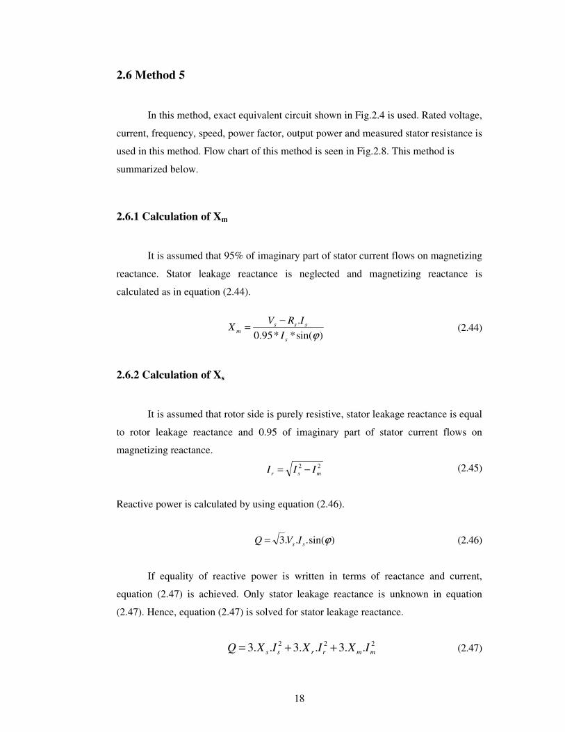
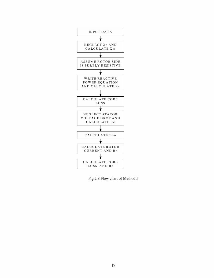
In this method, exact equivalent circuit shown in Fig.2.4 is used. Rated voltage,

current, frequency, speed, power factor, output power and measured stator resistance is

used in this method. Flow chart of this method is seen in Fig.2.8. This method is

summarized below.

2.6.1 Calculation of Xm

It is assumed that 95% of imaginary part of stator current flows on magnetizing

reactance. Stator leakage reactance is neglected and magnetizing reactance is

calculated as in equation (2.44).

(2.44)

2.6.2 Calculation of Xs

It is assumed that rotor side is purely resistive, stator leakage reactance is equal

to rotor leakage reactance and 0.95 of imaginary part of stator current flows on

magnetizing reactance.

(2.45)

Reactive power is calculated by using equation (2.46).

(2.46)

If equality of reactive power is written in terms of reactance and current,

equation (2.47) is achieved. Only stator leakage reactance is unknown in equation

(2.47). Hence, equation (2.47) is solved for stator leakage reactance.

(2.47)

19

N E G L E C T X s A N DC A L C U L A T E X m

A S S U M E R O T O R S ID EIS P U R E L Y R E S IS T IV E

W R IT E R E A C T IV EP O W E R E Q U A T IO N

A N D C A L C U L A T E X s

C A L C U L A T E C O R EL O S S

N E G L E C T S T A T O RV O L T A G E D R O P A N D

C A L C U L A T E R c

C A L C U L A T E T em

C A L C U L A T E R O T O RC U R R E N T A N D R r

C A L C U L A T E C O R EL O S S A N D R c

IN P U T D A T A

Fig.2.8 Flow chart of Method 5

20

RCLSCLlosscore PPPP −−=

ssincore RIs

PP ..3))1(

1.( 2−−

−= η

core

sc P

VR

2.3=

c

sssmsr R

IRVIII

).(22 −−−=

s

mecoutem s

PPT

ω).1( −+=

s

rem

sRrIT

ω/..3 2

=

2.6.3 Calculation of Rr

Initially core loss is calculated by using equation (2.49).

(2.48)

(2.49)

Stator voltage drop is neglected and Rc is calculated.

(2.50)

It is assumed that there is nearly 90º phase shift between magnetizing current

and referred rotor current. Then, referred rotor current is calculated from equation

(2.51)

(2.51)

It is assumed that mechanical losses and stray losses are equal to the 0.01 of

output power. Electromechanical torque is calculated by using equation (2.52).

(2.52)

If electromechanical torque is written as in equation (2.53), only referred rotor

resistance is unknown. Referred rotor resistance is calculated from equation (2.53).

(2.53)

2.6.4 Calculation of Rc

In this part, Rc value is corrected. Firstly, core loss is calculated from equation

(2.54).

21

.convstraySCLincore PPPPP −−−=

ϕ−∠+−= ssssm IXjRVE )..(

core

mc P

ER

2.3=

(2.54) Rc is calculated by substituting equation (2.55) into equation (2.56).

(2.55) (2.56)

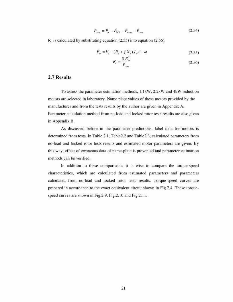
2.7 Results

To assess the parameter estimation methods, 1.1kW, 2.2kW and 4kW induction

motors are selected in laboratory. Name plate values of these motors provided by the

manufacturer and from the tests results by the author are given in Appendix A.

Parameter calculation method from no-load and locked rotor tests results are also given

in Appendix B.

As discussed before in the parameter predictions, label data for motors is

determined from tests. In Table 2.1, Table2.2 and Table2.3, calculated parameters from

no-load and locked rotor tests results and estimated motor parameters are given. By

this way, effect of erroneous data of name-plate is prevented and parameter estimation

methods can be verified.

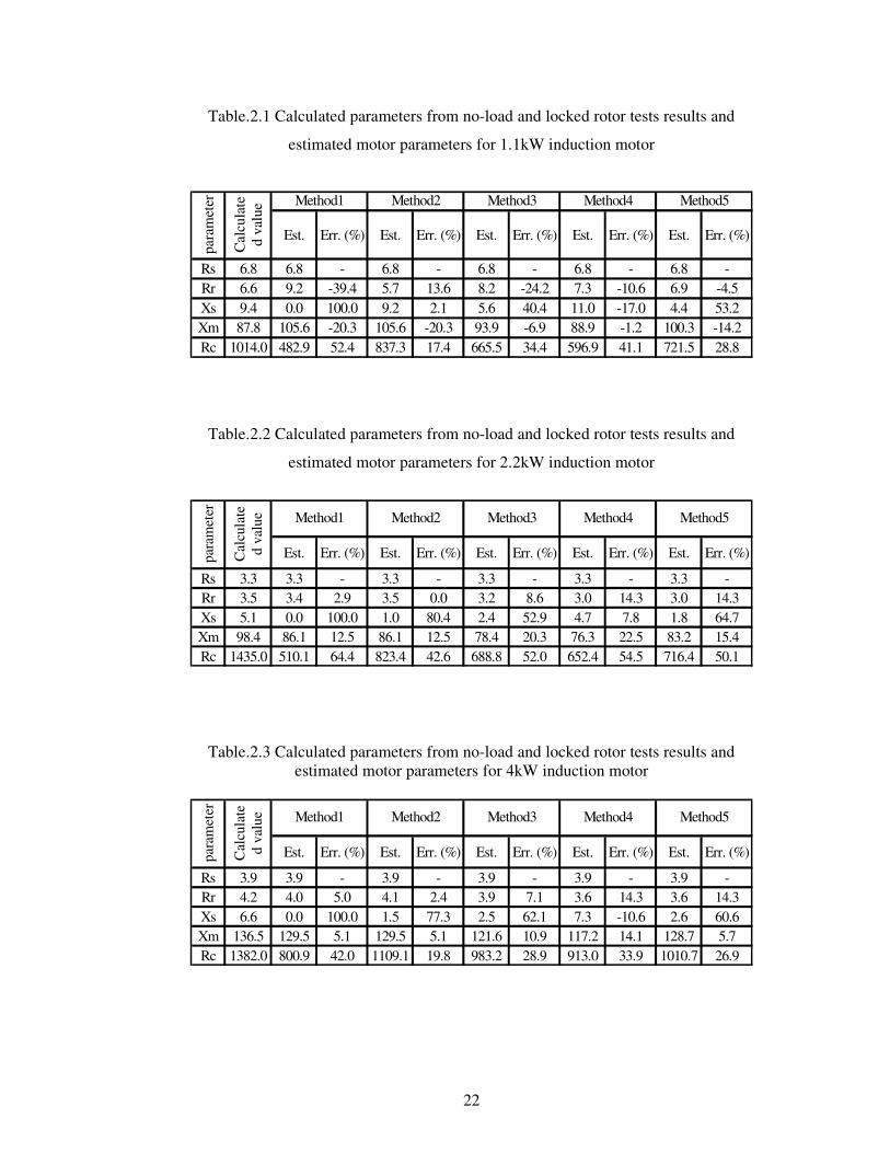
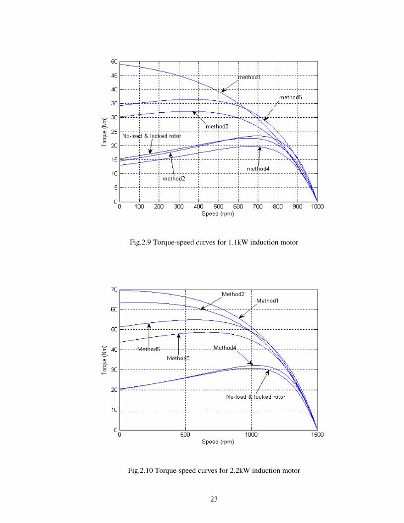
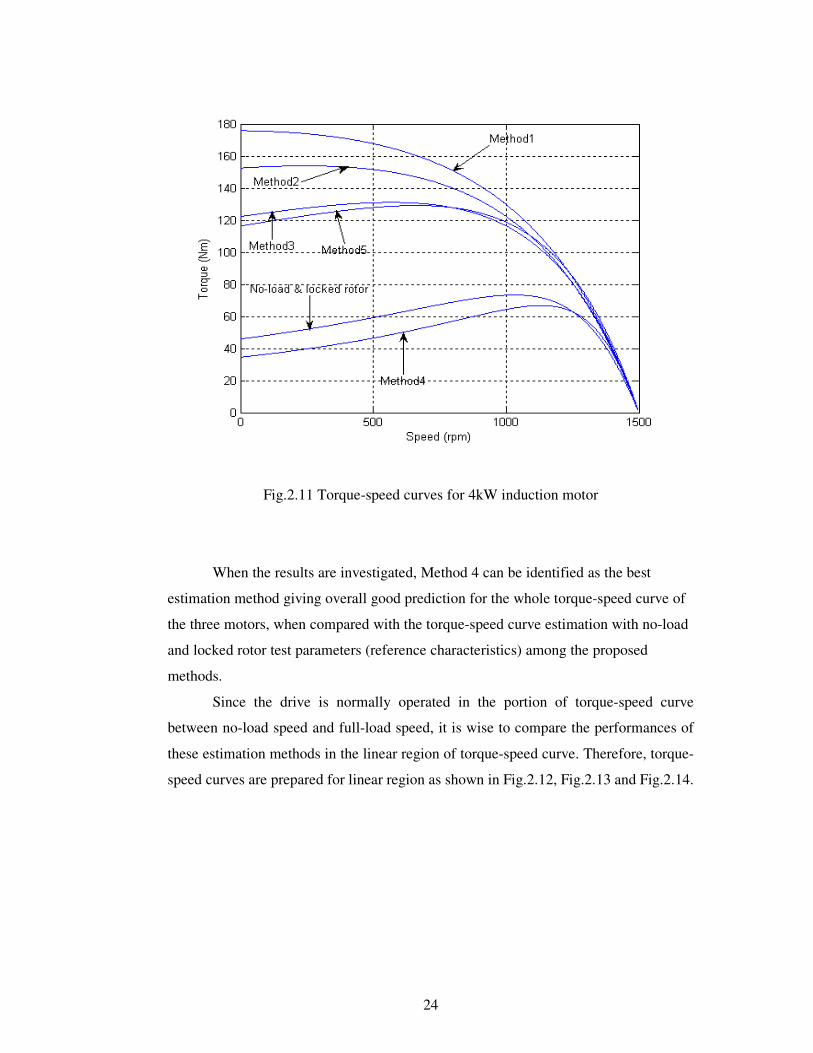
In addition to these comparisons, it is wise to compare the torque-speed

characteristics, which are calculated from estimated parameters and parameters

calculated from no-load and locked rotor tests results. Torque-speed curves are

prepared in accordance to the exact equivalent circuit shown in Fig.2.4. These torque-

speed curves are shown in Fig.2.9, Fig.2.10 and Fig.2.11.

22

Table.2.1 Calculated parameters from no-load and locked rotor tests results and

estimated motor parameters for 1.1kW induction motor

Est. Err. (%) Est. Err. (%) Est. Err. (%) Est. Err. (%) Est. Err. (%)

Rs 6.8 6.8 - 6.8 - 6.8 - 6.8 - 6.8 -Rr 6.6 9.2 -39.4 5.7 13.6 8.2 -24.2 7.3 -10.6 6.9 -4.5Xs 9.4 0.0 100.0 9.2 2.1 5.6 40.4 11.0 -17.0 4.4 53.2Xm 87.8 105.6 -20.3 105.6 -20.3 93.9 -6.9 88.9 -1.2 100.3 -14.2Rc 1014.0 482.9 52.4 837.3 17.4 665.5 34.4 596.9 41.1 721.5 28.8

para

met

er

Cal

cula

ted

valu

e Method1 Method2 Method3 Method4 Method5

Table.2.2 Calculated parameters from no-load and locked rotor tests results and

estimated motor parameters for 2.2kW induction motor

Est. Err. (%) Est. Err. (%) Est. Err. (%) Est. Err. (%) Est. Err. (%)

Rs 3.3 3.3 - 3.3 - 3.3 - 3.3 - 3.3 -Rr 3.5 3.4 2.9 3.5 0.0 3.2 8.6 3.0 14.3 3.0 14.3Xs 5.1 0.0 100.0 1.0 80.4 2.4 52.9 4.7 7.8 1.8 64.7Xm 98.4 86.1 12.5 86.1 12.5 78.4 20.3 76.3 22.5 83.2 15.4Rc 1435.0 510.1 64.4 823.4 42.6 688.8 52.0 652.4 54.5 716.4 50.1

para

met

er

Cal

cula

ted

valu

e Method1 Method2 Method3 Method4 Method5

Table.2.3 Calculated parameters from no-load and locked rotor tests results and estimated motor parameters for 4kW induction motor

Est. Err. (%) Est. Err. (%) Est. Err. (%) Est. Err. (%) Est. Err. (%)

Rs 3.9 3.9 - 3.9 - 3.9 - 3.9 - 3.9 -Rr 4.2 4.0 5.0 4.1 2.4 3.9 7.1 3.6 14.3 3.6 14.3Xs 6.6 0.0 100.0 1.5 77.3 2.5 62.1 7.3 -10.6 2.6 60.6Xm 136.5 129.5 5.1 129.5 5.1 121.6 10.9 117.2 14.1 128.7 5.7Rc 1382.0 800.9 42.0 1109.1 19.8 983.2 28.9 913.0 33.9 1010.7 26.9

Method3 Method4 Method5

para

met

er

Cal

cula

ted

valu

e Method1 Method2

23

Fig.2.9 Torque-speed curves for 1.1kW induction motor

Fig.2.10 Torque-speed curves for 2.2kW induction motor

24

Fig.2.11 Torque-speed curves for 4kW induction motor

When the results are investigated, Method 4 can be identified as the best

estimation method giving overall good prediction for the whole torque-speed curve of

the three motors, when compared with the torque-speed curve estimation with no-load

and locked rotor test parameters (reference characteristics) among the proposed

methods.

Since the drive is normally operated in the portion of torque-speed curve

between no-load speed and full-load speed, it is wise to compare the performances of

these estimation methods in the linear region of torque-speed curve. Therefore, torque-

speed curves are prepared for linear region as shown in Fig.2.12, Fig.2.13 and Fig.2.14.

25

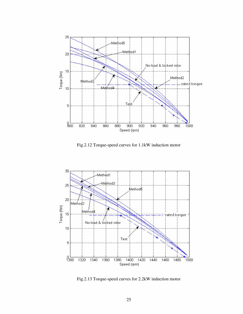
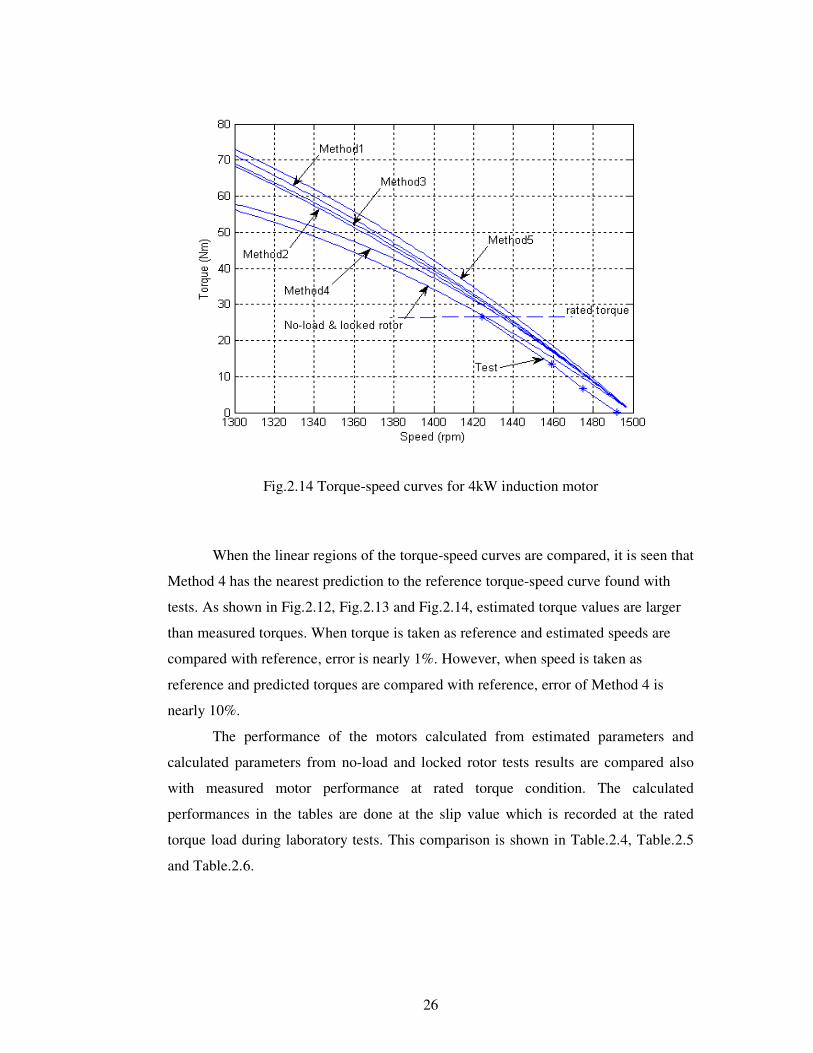
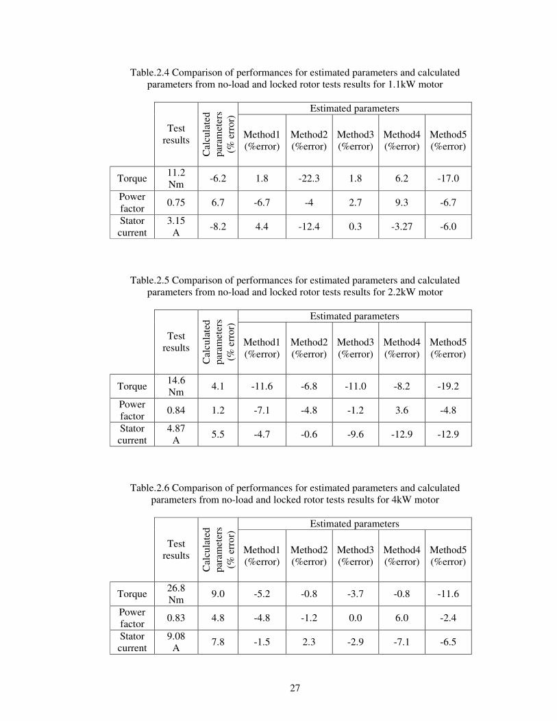
Fig.2.12 Torque-speed curves for 1.1kW induction motor

Fig.2.13 Torque-speed curves for 2.2kW induction motor

26

Fig.2.14 Torque-speed curves for 4kW induction motor When the linear regions of the torque-speed curves are compared, it is seen that

Method 4 has the nearest prediction to the reference torque-speed curve found with

tests. As shown in Fig.2.12, Fig.2.13 and Fig.2.14, estimated torque values are larger

than measured torques. When torque is taken as reference and estimated speeds are

compared with reference, error is nearly 1%. However, when speed is taken as

reference and predicted torques are compared with reference, error of Method 4 is

nearly 10%.

The performance of the motors calculated from estimated parameters and

calculated parameters from no-load and locked rotor tests results are compared also

with measured motor performance at rated torque condition. The calculated

performances in the tables are done at the slip value which is recorded at the rated

torque load during laboratory tests. This comparison is shown in Table.2.4, Table.2.5

and Table.2.6.

27

Table.2.4 Comparison of performances for estimated parameters and calculated parameters from no-load and locked rotor tests results for 1.1kW motor

Estimated parameters

Test results

Cal

cula

ted

para

met

ers

(% e

rror

)

Method1 (%error)

Method2 (%error)

Method3 (%error)

Method4 (%error)

Method5 (%error)

Torque 11.2 Nm -6.2 1.8 -22.3 1.8 6.2 -17.0

Power factor 0.75 6.7 -6.7 -4 2.7 9.3 -6.7

Stator current

3.15 A -8.2 4.4 -12.4 0.3 -3.27 -6.0

Table.2.5 Comparison of performances for estimated parameters and calculated parameters from no-load and locked rotor tests results for 2.2kW motor

Estimated parameters

Test results

Cal

cula

ted

para

met

ers

(% e

rror

)

Method1 (%error)

Method2 (%error)

Method3 (%error)

Method4 (%error)

Method5 (%error)

Torque 14.6 Nm 4.1 -11.6 -6.8 -11.0 -8.2 -19.2

Power factor 0.84 1.2 -7.1 -4.8 -1.2 3.6 -4.8

Stator current

4.87 A 5.5 -4.7 -0.6 -9.6 -12.9 -12.9

Table.2.6 Comparison of performances for estimated parameters and calculated parameters from no-load and locked rotor tests results for 4kW motor

Estimated parameters

Test results

Cal

cula

ted

para

met

ers

(% e

rror

)

Method1 (%error)

Method2 (%error)

Method3 (%error)

Method4 (%error)

Method5 (%error)

Torque 26.8 Nm 9.0 -5.2 -0.8 -3.7 -0.8 -11.6

Power factor 0.83 4.8 -4.8 -1.2 0.0 6.0 -2.4

Stator current

9.08 A 7.8 -1.5 2.3 -2.9 -7.1 -6.5

28

resulttestvalueestimatedresulttest

error.

..%

−=

In Table.2.4, Table.2.5 and Table.2.6, error is defined as in equation (2.57).

(2.57)

In the evaluation of performances for estimated motor parameters, average of

the error is considered. When Table.2.4 is investigated, it is shown that Method 3 and

Method 1 are better than other methods for 1.1kW motor. It is shown in Table.2.5 that

Method 2 is better than other methods for 2.2kW motor. For 4kW motor, Method 2 and

Method 3 are more suitable than other methods. When all test motors are considered,

Method 3 can be identified as the best estimation method amongst these methods.

Computational burden of parameter estimation methods is assessed in

Table.2.7.

Table.2.7 Computational burden of parameter estimation methods

Method3 Method4

Method1 Method2 Initial

Comp.

loop Initial

Comp.

loop

Method5

Number of multiplications

33 25 9 48 10 66 66

Number of additions

6 3 3 5 3 10 4

Number of subtractions

12 9 7 7 8 8 18

Number of divisions

18 13 3 10 4 13 14

Number of square roots

3 1 1 4 2 4 4

To calculate the computation time of each method, DSPIC30F6010 (40 MHz)

is taken as reference. Method 4 is assumed to be finalized in 6 iterations. It is seen that

calculation time of Method 4 and Method 3 are nearly 10 ms and others are nearly 2

ms1. Computation times of Method 4 and Method 3 are larger than others. However,

1 Multiplications, additions and subtractions are done in 1 instruction cycle. Division is assumed to be done in 20 instruction cycle and square root is assumed to be done in 500 �s.

29

parameter estimation is done at the initialization of motor drive and computation times

of all methods are in the acceptable range.

To investigate the effect of erroneous data of name-plate for calculation of

motor parameters and preparation of torque-speed curve, motor parameters are

estimated from name-plate data and torque-speed curves are prepared in accordance to

these parameters. Estimated parameters and prepared torque speed curves are shown in

Appendices.

30

CHAPTER 3

PREDICTION OF MOTOR SPEED

3.1 Introduction

In industrial drives market, requirements related to control quality and price of

drives are important. To reduce the initial cost of the low cost motor drives, it is

necessary to use low performance microprocessors. Since price of the microprocessor

is proportional to the performance of the microprocessor, in low cost drives one of the

aims is achieving speed estimation accuracy with minimum number of calculations.

Speed estimation techniques depend on motor parameters. These motor

parameters can be predicted from manufacturer data or measured. On-line

measurement of parameters places an important burden on the microprocessor. For that

reason, low cost drives avoid this approach and often estimate parameters from the user

supplied motor label data.

The purpose of this section is to investigate methods of speed estimation in the

literature and find out whether a more accurate and less computation intensive method

can be developed. Various methods of speed estimation techniques are described in

literature. The most common method used in practice is linearization of torque-speed

curve [5][10]. This method is explained below as Method 3. Only base frequency,

speed, output power, number of poles and stator resistance are used in this method.

These data are obtained at base frequency and rated torque. Since the number of

calculations is very low, this method can be applied with low performance

microprocessors. This method has drawbacks at high loads and in the field weakening

region as explained in Method 3. In [10], it is reported that when this method is applied

31

to a 3.7 kW induction motor whose stator resistance is 0.114�, speed is estimated with

5% error at 20Hz under full load [10].

Another speed estimation method, which does not require motor parameters

except stator resistance, is based on a non-linear relationship between air-gap power

and slip speed [6]. This method is explained below as Method 1. Base frequency,

voltage, current, speed, power factor, output power, number of poles, efficiency,

breakdown torque at base frequency and stator resistance are used in Method 1. These

data are obtained at base frequency and rated torque. When this method is applied to

3hp induction motor whose stator resistance is 0.89�, in [10] it is found that speed is

estimated with 1% error at 10Hz under full load condition [6]. In this method, since the

breakdown torque is assumed to be constant and stator resistance is neglected at

calculation of slip speed, this method is not suitable for high speeds and small motors,

at which voltage drop on the stator resistance is comparable to input voltage at low

frequencies. For low hp motors, to obtain good speed prediction accuracy, methods

must be developed taking into account the stator resistance.

When the methods in the literature are investigated, it is observed that each

method has advantages and disadvantages. Therefore, it is decided to investigate the

level of accuracy that may be expected from these approaches and possibly develop a

more accurate approach with similar computation burden.

In this Chapter, both the existing speed estimation methods and proposed speed

estimation methods are examined on 1.1 kW, 2.2 kW and 4kW induction motors.

First to verify the used circuit model, motor is driven with line voltage and

calculated torque from model is compared with measured torque. That shows the best

accuracy acceptable with this model.

Since the methods studied here are to be used in applications where the speed is

controlled, it is essential to use an inverter. Many methods require measurement of

voltage and current. Measurement of these variables affects the accuracy of

predictions. For that reason, the current and voltage measurement circuits used are

calibrated and measurement accuracy is investigated at different frequencies.

As the next step accuracy of the model is investigated while the three test

motors are driven at 10Hz, 30Hz, 50Hz and 70Hz. Hence, idea of the accuracy of the

model used is obtained for a frequency range of (10Hz-70Hz). This issue is

investigated in Chapter5.

32

In this study, medium frequency is defined as between 20 Hz and 50 Hz.

Frequencies over 50 Hz are named as high frequency. Low frequency is defined as

below 20Hz in this study. Since 1.1kW, 2.2kW and 4 kW motors are available in

laboratory and the capacity of the inverter is not suitable for larger motors, these

motors are used in the experiments. In this study, 1.1 kW motor is named as small

motor and 4kW motor is named as large motor.

Any method for speed prediction is based on the model investigated. The best

accuracy of prediction may be expected when the exact model is used. However, this

would bring too much computational burden and would require knowledge of all the

parameters. For this reason, all the methods involve some degree of approximation.

Therefore, it is wise to compare the speed estimation of a method with the speed

estimation from the exact equivalent circuit.

To make realistic predictions, the simulations are made using the current and

voltage values measured during tests. Therefore, any error that may be introduced due

to the measurements of these variables is taken into account in these predictions. For

the prediction Matlab environment is used. The Matlab model is described in Chapter

4.

In the following sections, each of the methods proposed in the literature and

improvements proposed by the author are described.

3.2 Investigation of speed estimation methods

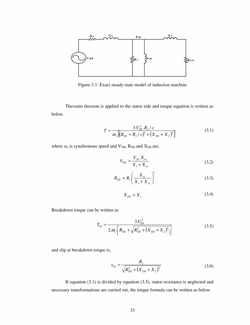
3.2.1 Method 1

In this method, exact steady-state circuit model is used. This method is based

on a non-linear relationship between air-gap power and slip speed [6]. Base frequency,

voltage, current, power factor, speed, number of poles, efficiency, output power,

breakdown torque and stator resistance are used in this method. These data are

obtained at the base frequency and rated torque. Instantaneous stator currents are

measured in two phases. Output voltage of the inverter is assumed to be equal to the

reference voltage. Method is summarized below.

33

( ) ( )[ ]22

22

22

/./..3

XXsRRsRV

TTHTHs

TH

+++=

ω

m

mphTH XX

XVV

+=

1

.

2

11. ��

�

����

�

+=

m

mTH XX

XRR

1XXTH =

( ) ��

�� +++

=2

22

2

..2

.3

XXRR

VT

THTHTHs

THbd

ω

( )22

2

2

XXR

Rs

THTH

bd++

=

V p h

X sR s

R c X m

X r

R r /s

E m

Figure.3.1: Exact steady-state model of induction machine

Thevenin theorem is applied to the stator side and torque equation is written as

below.

(3.1)

where s is synchronous speed and VTH, RTH and XTH are,

(3.2)

(3.3)

(3.4)

Breakdown torque can be written as

(3.5)

and slip at breakdown torque is,

(3.6)

If equation (3.1) is divided by equation (3.5), stator resistance is neglected and

necessary transformations are carried out, the torque formula can be written as below.

34

ss

ss

TT

bd

bd

bd

+= .2

���

�

����

���−−=

2

.11...

Ro

L

L

RRo

TKT

TsTKK

s

R

bdo T

TK =

12 −+== ooR

bd KKss

K

s

gapL

PT

ω=

(3.7)

If this equation is solved, slip is,

(3.8)

Where sR is slip at rated torque condition and Ko, K and TL are,

(3.9)

(3.10)

(3.11)

In equation (3.11), air-gap power is calculated by subtracting the stator copper

loss and core loss from input power. In the application of this method, equation (3.8)

shows a non-linear relationship between air-gap power and slip. Ko, TR and sR values

are found from motor catalogue data. K and TL are calculated from equation (3.10) and

(3.11) respectively. Finally slip is calculated from equation (3.8).

In this method, Ko is assumed to be constant. To satisfy this assumption, flux

linkage must be kept constant at rated value. However, at high frequencies motor is in

the field weakening region and flux linkage value is lower than rated value. Therefore,

this method is not suitable for high frequencies.

Generally stator resistance of small motors is high and voltage drop on the

stator resistance is comparable to input voltage at low frequencies. Since stator

resistance is neglected in this method, this method is not suitable for small motors at

low frequencies. However, stator resistance is generally small and voltage drop on the

stator resistance can be neglected in large motors. Hence, this method can be used for

large motors at low frequencies.

35

The validity of the assumptions at medium frequency is somewhere in between

the low frequency and high frequency cases. Suitable types of motors and frequencies

for this method are shown in Table.3.1.

Table.3.1 Suitable types of motors and frequencies for Method 1

Frequency

Low Medium High Small motors X Large motors X X

The computational burden of the method is assessed in Table.3.2.

Table.3.2 Calculation burden of Method 1

Number of multiplications 54

Number of divisions 19

Number of additions 9

Number of subtractions 9

Number of square roots 1 In view of Table.3.2 it can be concluded that, using of a high performance

processor is obligatory in this approach. Since this method does not require any motor

parameters except stator resistance, this method can be applied easily.

3.2.2 Method 2

To improve the performance of Method 1 in the field weakening region, this

method is proposed. Philosophy of this method is same with Method 1. Base

frequency, voltage, current, speed, power factor, output power, number of poles,

36

r

bdo T

TK =

( )��

�� +++

=2

22

2

..2

.3

XXRR

VT

THTHTHs

THbd

ω

efficiency, breakdown torque, stator resistance, magnetizing reactance and stator

leakage reactance are used in this method. These data are obtained at base frequency

and rated torque. Instantaneous stator currents are measured in two phases. Output

voltage of the inverter is assumed to be equal to the reference voltage. This method is

summarized below.

As explained in Method 1, Ko value is changing in the field weakening region.

To improve the performance of Method 1 especially in the field weakening region,

calculated breakdown torque from equation (3.13) is used instead of assuming Ko be

constant. Ko is calculated as below.

(3.12)

where Tr is rated torque and breakdown torque explained above is

(3.13)

In the application of this method, breakdown torque is calculated from equation

(3.13) where VTH, RTH and XTH are calculated from equation (3.2), (3.3) and (3.4)

respectively. By using calculated breakdown torque, Ko is calculated from equation

(3.12) and rest of the calculations are same with Method 1.

Correction of Ko value is expected to improve the performance of this

speed estimation method. This method is suitable for large and small motors at high

frequencies. Suitable types of motors and frequencies for this method are shown in

Table.3.3.

Table.3.3 Suitable types of motors and frequencies for Method 2

Frequency

Low Medium High Small motors X X Large motors X X X

37

( )22

2 ..2

.3

lrsl

r

sl

r

m

LR

Rp

T

+���

����

�

���

����

�

=

ω

ωλ

Table.3.4 Calculation burden of Method 2

Number of multiplications 63

Number of divisions 23

Number of additions 13

Number of subtractions 9

Number of square roots 2 In Table.3.4, calculation burden contains calculation of breakdown torque.

However, breakdown torque is calculated only one time for each voltage and

frequency. Therefore, calculation burden of Method 2 is assumed to be equal to the

calculation burden of Method 1. However, Method 2 requires more motor parameters.

For this reason, application of Method 2 is more difficult than Method 1.

3.2.3 Method 3

This method investigated here is one of the most commonly used methods in

low cost application. In this method, torque-speed curve is assumed to be linear. This

method uses only base speed, output power, frequency, number of poles and stator

resistance. These data are obtained at base frequency and rated torque. Voltage and

current are measured. This method is summarized below.

In [5], torque equation is written as in equation (3.14).

(3.14)

where mλ denotes flux linkage, p denotes number of poles and lrL denotes rotor

leakage reactance. Equation (3.14) shows that torque is proportional to slip if flux

linkage is kept constant at rated value where motor parameters are assumed to be

constant. If these assumptions are existing, slopes of torque-speed curves are parallel

and slip speed can be calculated from equation (3.15).

38

slrR

Lsl n

TT

n .���

����

�= (3.15)

where nslr is slip speed at rated condition, TR is rated torque and TL is load torque. In

the application of this method, TL calculated from equation (3.11) is inserted to

equation (3.15) and slip speed is calculated.

If this method is investigated, it is seen that this method has some drawbacks.

One of these drawbacks occurs in the field weakening region. As explained in Method

1, flux linkage is reduced in the field weakening region. Therefore, slope of the torque-

speed curve is changing as seen in equation (3.14). Therefore, it is expected that error

ratio of this method is increasing in the field weakening region.

Another drawback of this method is that slope of torque-speed curve is

dependent on change of motor parameters with temperature. Equation (3.14) shows

that if rotor winding temperature is increased, slip speed is increased to reach the same

torque.

Another drawback of this method is that erroneous data of the motor name-

plate is reflected to estimation results. Although this drawback is valid for all speed

estimation methods, effect of this drawback to the estimation result is weak in other

methods. In other methods, motor name-plate data are used to calculate core-loss at

base frequency and rated torque. Therefore, effect of erroneous data in name-plate is

seen as weaker while calculating air-gap power. However, in this method, erroneous

data of name-plate causes high errors at low frequencies.

If these drawbacks are taken into account, it is seen that this method may have

large errors at low speeds and in the field weakening region. Suitable types of motors

and frequencies for this method are shown in Table.3.5.

Table.3.5 Suitable types of motors and frequencies for Method 3

Frequency

Low Medium High Small motors X Large motors X

39

Table.3.6 Calculation burden of Method 3

Number of multiplications 31

Number of divisions 15

Number of additions 4

Number of subtractions 9

Number of square roots -

Although performance of this method is expected to be worse than Method 1

and Method 2, this method is one of the most commonly used methods in literature

because of low computational burden and ease of application.

It is possible to improve the low speed and high speed performance of this

method by using some of the motor parameters. However, no suggestions is made in

this study to improve this method. Penalty of these improvements is increase of the

computational burden and this reduces the attractiveness of this method.

3.2.4 Method 4

To improve the performance of Method 1, Method 2 and Method 3 in the field

weakening region and at low frequencies, this method is proposed. This method is

based on the relation between torque and slip. In Method 1, breakdown torque is

assumed to be constant. However, in this method, breakdown torque is calculated for

each voltage and frequency case. Torque equations are derived regarding to the stator

resistance. For these reasons, this method is expected to perform better than Method 1,

Method 2 and Method 3 in the field weakening region and at low frequencies.

In this method, base frequency, voltage, current, speed, power factor, output

power, number of poles, efficiency and all motor parameters are used. These data are

obtained at base frequency and rated torque. Voltage and two phase instantaneous

currents are measured. This method is summarized below.

40

( ) ( )[ ]221

221

22

/./..3

XXsRRsRV

Ts

s

+++=

ω

( ) ��

�� +++

=2

212

11

2

..2

.3

XXRR

VT

s

sbd

ω

( )221

21

2

XXR

Rsbd

++=

( )bd

bd

bd

bdbd

sas

sss

saTT

..2

.1..2

++

+=

2

1

RR

a =

X1R1

R c X m

X2

R2/s

Figure.3.2. Approximate model of induction machine

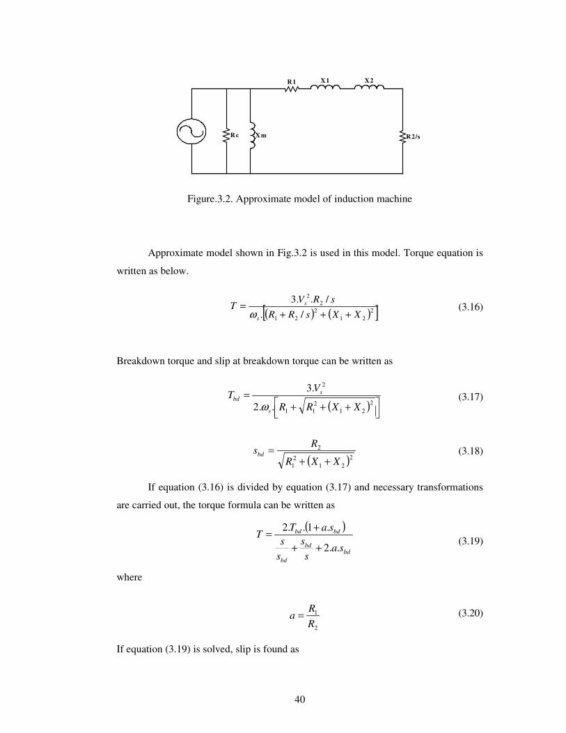
Approximate model shown in Fig.3.2 is used in this model. Torque equation is

written as below.

(3.16)

Breakdown torque and slip at breakdown torque can be written as

(3.17)

(3.18)

If equation (3.16) is divided by equation (3.17) and necessary transformations

are carried out, the torque formula can be written as

(3.19)

where

(3.20)

If equation (3.19) is solved, slip is found as

41

[ ]1. 2 −−= bbss bd

( )L

Lbdbdbd

TTsasaT

b...1. −+=

(3.21)

where

(3.22)

In the application of this method, Tbd, TL and sbd are calculated from equation

(3.17), (3.11) and (3.18) respectively. Then a and b are calculated from equation (3.20)

and (3.22) respectively. Slip is calculated from equation (3.21).

This method can be shown to lead to the same equation ((3.21) and (3.22)), if in

the derivation, the exact equivalent circuit is considered and the stator leakage

reactance is neglected. Therefore, it is possible to conclude at high frequencies, speed

predictions are likely to be erroneous.

Since stator resistance is taken into account when torque equations are derived,

this method is expected to give better results at low frequencies. Suitable types of

motors and frequencies for this method are shown in Table.3.7.

Table.3.7 Suitable types of motors and frequencies for Method 4

Frequency

Low Medium High Small motors X X Large motors X X

Table.3.8 Calculation burden of Method 4

Number of multiplications 56

Number of divisions 22

Number of additions 10

Number of subtractions 11

Number of square roots 3

42

( ) ( )[ ]22

22

22

/./..3

XXsRRsRV

TTHTHs

TH

+++=

ω

( ) ��

�� +++

=2

22

2

..2

.3

XXRR

VT

THTHTHs

THbd

ω

( )22

2

2

XXR

Rs

THTH

bd++

=

( )bd

bd

bd

bdbd

sas

sss

saTT

..2

.1..2

++

+=

If calculation burden of this method is investigated, it is seen that numbers of

calculations are similar to Method 1 and Method 2.

Since all motor parameters are used in this method, application of this method

is more difficult than Method 1 and Method 2.

3.2.5 Method 5

To improve the performance of Method 4 at high frequencies, this method is

improved. In this method, exact circuit model is used. Philosophy of the method is

same with Method 4. Since stator leakage reactance is taken into account in this

method, this method is expected to give better results than Method 4. In this method,

base frequency, voltage, current, speed, power factor, output power, number of poles

and all motor parameters are used. These data are obtained at base frequency and rated

torque. In this method, voltage and two phase instantaneous currents are measured.

This method is summarized below.

Torque equation can be written as

(3.23)

Breakdown torque and slip at breakdown torque can be written as

(3.24)

(3.25)

where VTH, RTH and XTH are calculated from equation (3.2), (3.3) and (3.4)

respectively.

If equation (3.23) is divided by equation (3.24) and necessary transformations

are carried out, the torque formula can be written as

(3.26)

43

2RR

a TH=

[ ]1. 2 −−= bbss bd

( )L

Lbdbdbd

TTsasaT

b...1. −+=

where

(3.27)

If equation (3.26) is solved, slip is found as

(3.28)

where

(3.29)

In the application of this method, VTH, RTH and XTH are calculated from

equation (3.2), (3.3) and (3.4) respectively. Then Tbd, TL and sbd are calculated from

equation (3.24), (3.11) and (3.25) respectively. Then a and b are calculated from

equation (3.27) and (3.29). Finally, slip is calculated from equation (3.28).

Since load torque and breakdown torque equations are derived in accordance to

the exact steady-state equivalent circuit, this method is expected to be suitable for all

frequencies and motor types. This method is expected to give the same results with

simulation of the motor model. Suitable types of motors and frequencies for this

method are shown in Table.3.9.

Table.3.9 Suitable types of motors and frequencies for Method 5

Frequency

Low Medium High Small motors X X X Large motors X X X

44

Table.3.10 Calculation burden of Method 5

Number of multiplication 56

Number of division 22

Number of addition 10

Number of subtraction 11

Number of square roots 3 If calculation burden of this method is investigated, it is seen that number of

calculations is similar to Method 4. That all parameters are used in this method is

shown as disadvantage of this method.

3.2.6 Method 6

To improve the performance of Method 1 and Method 3 at low frequencies, this

method is proposed. To minimize the effect of stator resistance, equivalent circuit is

modified. This method is based on the relation between slip and torque equations.

Torque equations are derived in accordance to the modified equivalent circuit.

Philosophy of this method is similar to Method 4.

Base frequency, voltage, current, speed, power factor, output power, efficiency,

number of poles, breakdown torque and all motor parameters are used in this method.

These data are obtained at base frequency and rated torque. Voltage and two phase

instantaneous currents are measured. This method is summarized below.

Modified equivalent circuit shown in Fig.3.3 does not contain stator resistance.

Input voltage (es) value is changing in accordance to the slip and phase current. es is

calculated by subtracting the voltage drop on the stator resistance from input voltage.

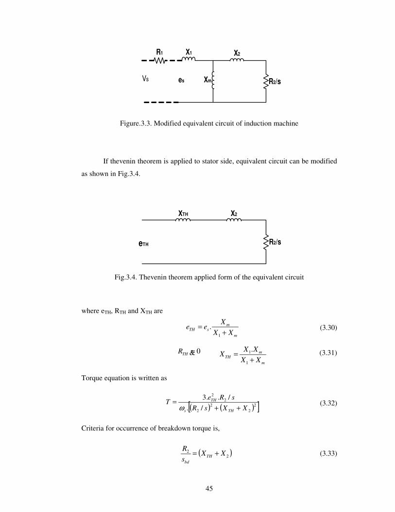
45

m

msTH XX

Xee

+=

1

.

0=THRm

mTH XX

XXX

+=

1

1.

( ) ( )[ ]22

22

22

/./..3

XXsRsRe

TTHs

TH

++=

ω

( )22 XX

sR

THbd

+=

X1

Xm

X2

R2/ses

R1

Vs

Figure.3.3. Modified equivalent circuit of induction machine

If thevenin theorem is applied to stator side, equivalent circuit can be modified

as shown in Fig.3.4.

XTH X2

R2/seTH

Fig.3.4. Thevenin theorem applied form of the equivalent circuit where eTH, RTH and XTH are (3.30)

& (3.31)

Torque equation is written as

(3.32)

Criteria for occurrence of breakdown torque is,

(3.33)

46

m

msbdTHbd XX

Xee

+=

1

.

0=THbdRm

mTHbd XX

XXX

+=

1

1.

1XXTH =

ss

ss

Tee

Tbd

bd

bd

sbd

s

+���

����

�= .2

.2

( )2

2

..2.3

XXe

TTHbds

THbdbd +

=ω

[ ]1. 2 −−= bbss bd

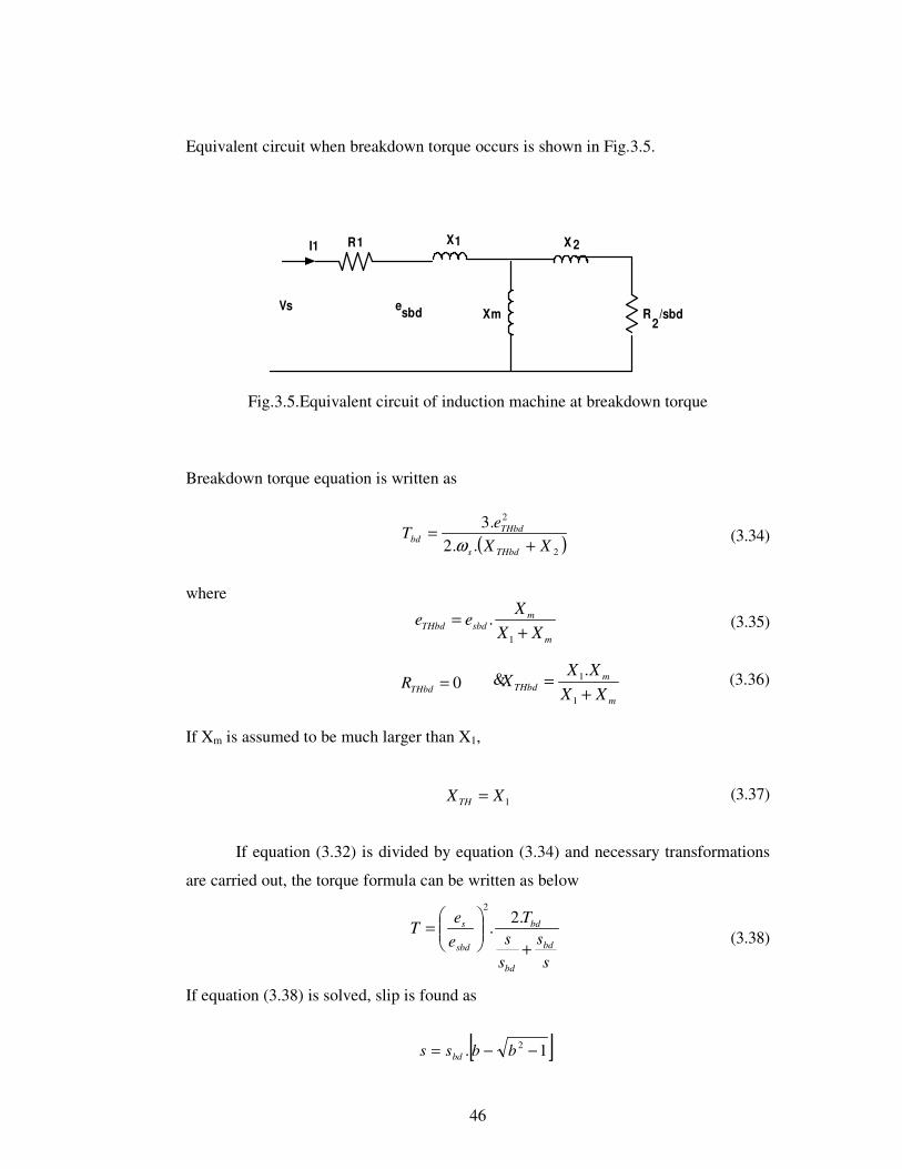
Equivalent circuit when breakdown torque occurs is shown in Fig.3.5.

X1

Xm

X 2

R2

/sbdesbd

R1

Vs

I1

Fig.3.5.Equivalent circuit of induction machine at breakdown torque Breakdown torque equation is written as

(3.34)

where

(3.35)

& (3.36)

If Xm is assumed to be much larger than X1,

(3.37)

If equation (3.32) is divided by equation (3.34) and necessary transformations

are carried out, the torque formula can be written as below

(3.38)

If equation (3.38) is solved, slip is found as

47

L

bdsbds

TTee

b.)/( 2

=

11.IRVe ssbd −=

(3.39)

where

(3.40)

The most critical point in this method is the estimation of esbd value at

breakdown torque condition. esbd is calculated from equation (3.41).

Eq.3.41

where 1I denotes stator current and can be calculated by dividing the equivalent

impedance of circuit shown in Fig.3.5 to the input voltage.

In the application of this method, es and esbd are calculated from equation

(3.41). sbd and Tbd are calculated from equation (3.6) and (3.5) respectively. TL is

calculated from equation (3.11). Finally slip is calculated from equation (3.39).

In the calculation of es and esbd, stator current is assumed to be in phase with

input voltage. Therefore, this method is expected to calculate es and esbd lower than

actual values of es and esbd. For this reason, it is expected that the error of this method

is increasing at low speeds. At high frequencies, reactance of the equivalent circuit is

dominant. Therefore, this approximation increases the error ratio of this method at high

frequencies. Despite of erroneous assumptions, this method can be used for all

frequencies, since effect of stator resistance and reducing flux linkage in the field

weakening region are taken into account. Suitable types of motors and frequencies for

this method are shown in Table.3.11.

Table.3.11 Suitable types of motors and frequencies for Method 6

Frequency

Low Medium High Small motors X X X Large motors X X X

Table.3.12 Calculation burden of Method 6

48

s

gapPT

ω=

bdgap sRIP /**3 222=

22 *3

**R

sTI sbdbd ω

=

Number of multiplications 54

Number of divisions 22

Number of additions 10

Number of subtractions 12

Number of square roots 3 If calculation burden of this method is investigated, it is shown that number of

calculations is similar to Method 4. Since all motor parameters are used as in Method

4, application of this method is more difficult than Method 1 and Method 3.

3.2.7 Method 7

To improve the performance of Method 6, it is necessary to estimate esbd

accurately. Therefore, a different approach for calculation of esbd is proposed in this

method. Philosophy of the method is same with Method 6. Only the estimation of esbd

is different from Method 6. Base frequency, voltage, current, speed, power factor,

output power, efficiency, number of poles, breakdown torque and all motor parameters

are used in this method. These data are obtained at the base frequency and rated torque.

Voltage and two phases instantaneous currents are measured. This method is

summarized below.

To find esbd, referred rotor current is estimated. Torque equation can be written

as below

(3.42)

where air-gap power is,

(3.43)

From equation (3.42) and (3.43), referred rotor current at breakdown torque condition

can be written as below.

(3.44)

49

( )2

22

2

*3**

*R

sTX

sR

e sbdbds

bdsbd

ω+��

�

����

�=

Neglecting voltage drop on the stator leakage reactance, esbd can be calculated from

equation (3.45).

(3.45)

In the application of this method, sbd and Tbd are calculated from equation (3.6)

and (3.5) respectively. es and esbd are calculated from equation (3.41) and (3.45)

respectively. TL is calculated from equation (3.11). Finally, slip is calculated from

equation (3.39).

Since stator resistance is taken into account, this method is expected to give

better results than Method 1. In the calculation of es, stator current is assumed to be in

phase with input voltage. Therefore, this method is expected to calculate es lower than

actual value of es. For this reason, it is expected that error of this method is increasing

at low speeds. At high frequencies, neglecting voltage drop on the stator leakage

reactance while calculating esbd increases the error ratio of this method. Even if the

error ratio of this method is increasing at high frequencies, speed estimation results of

this method are also acceptable. Suitable types of motors and frequencies for this

method are shown in Table.3.13.

Table.3.13 Suitable types of motors and frequencies for Method 7

Frequency

Low Medium High Small motors X X Large motors X X

Table.3.14 Calculation burden of Method 7

Number of multiplications 54

Number of divisions 22

Number of additions 7

Number of subtractions 13

Number of square roots 5

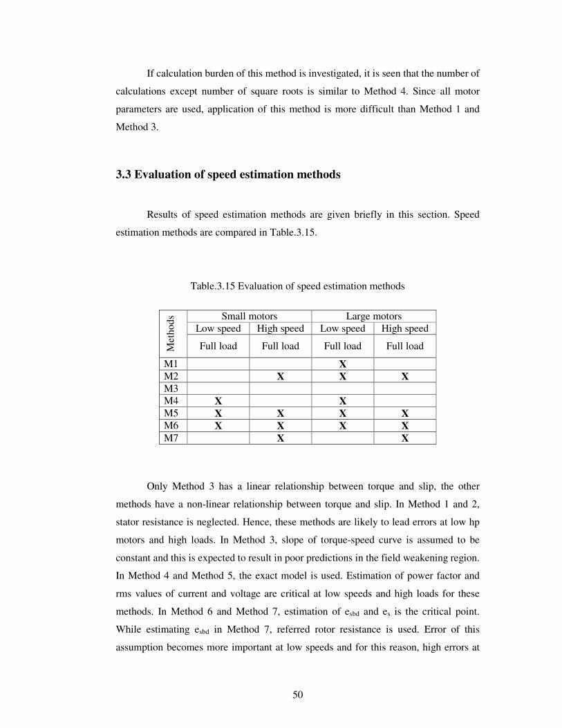
50

If calculation burden of this method is investigated, it is seen that the number of

calculations except number of square roots is similar to Method 4. Since all motor

parameters are used, application of this method is more difficult than Method 1 and

Method 3.

3.3 Evaluation of speed estimation methods

Results of speed estimation methods are given briefly in this section. Speed

estimation methods are compared in Table.3.15.

Table.3.15 Evaluation of speed estimation methods

Small motors Large motors

Low speed High speed Low speed High speed

Met

hods

Full load Full load Full load Full load

M1 X M2 X X X M3 M4 X X M5 X X X X M6 X X X X M7 X X

Only Method 3 has a linear relationship between torque and slip, the other

methods have a non-linear relationship between torque and slip. In Method 1 and 2,

stator resistance is neglected. Hence, these methods are likely to lead errors at low hp

motors and high loads. In Method 3, slope of torque-speed curve is assumed to be

constant and this is expected to result in poor predictions in the field weakening region.

In Method 4 and Method 5, the exact model is used. Estimation of power factor and

rms values of current and voltage are critical at low speeds and high loads for these

methods. In Method 6 and Method 7, estimation of esbd and es is the critical point.

While estimating esbd in Method 7, referred rotor resistance is used. Error of this

assumption becomes more important at low speeds and for this reason, high errors at

51

low speeds may be expected. While estimating es in Method 6, current is assumed to be

in phase with input voltage. However, this assumption increases the error at low

frequencies. Since only stator resistance and motor name-plate data are used and

number of calculations is low, Method 3 is the easiest method to be applied on a motor

drive. Table.3.39 and Table.3.40 show that if dc shift on current is prevented, error

ratios of all methods are reducing. Although dc shift on stator current worsens the

estimation of rms value of current and power factor, results of Method 4, Method 5 and

Method 6 are not worsened as much as the results of other methods.

52

CHAPTER 4

SIMULATION AND EXPERIMENTAL WORK

4.1 Introduction

Initially hardware and software, which are used in the experiments, are briefly

explained in this chapter. Then, calibration of voltage measurement module, current

measurement module and calibration of torquemeter are explained shortly. Then,

measurement of rotational loss is explained. In speed estimation algorithms, core loss,

rms value of current, rms value of voltage and power factor are estimated. In this

chapter, these estimations are verified. Finally, simulation of motor model in Matlab is

explained.

4.2 Hardware

Hardware used in experiments consists of DSP board, lock-out module,

isolation module, IPM, current and voltage measurement modules and power stage.

The block diagram of hardware is shown in Figure.4.1.

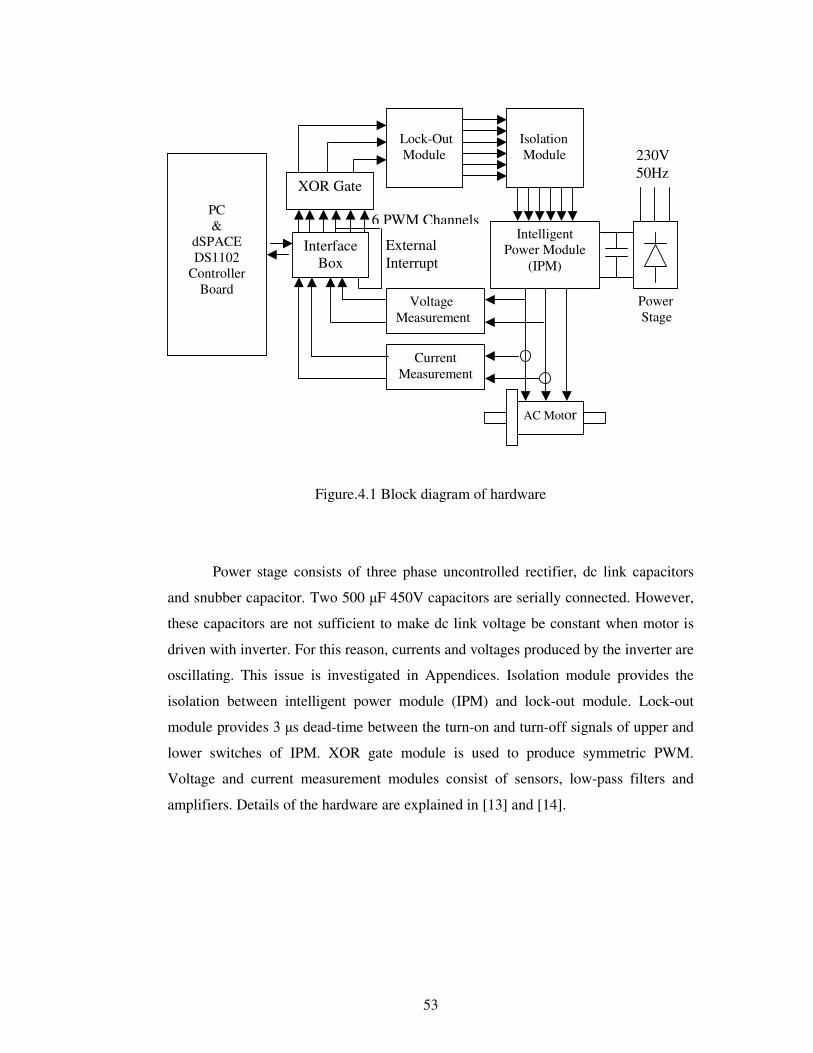
53

Figure.4.1 Block diagram of hardware

Power stage consists of three phase uncontrolled rectifier, dc link capacitors

and snubber capacitor. Two 500 �F 450V capacitors are serially connected. However,

these capacitors are not sufficient to make dc link voltage be constant when motor is

driven with inverter. For this reason, currents and voltages produced by the inverter are

oscillating. This issue is investigated in Appendices. Isolation module provides the

isolation between intelligent power module (IPM) and lock-out module. Lock-out

module provides 3 �s dead-time between the turn-on and turn-off signals of upper and

lower switches of IPM. XOR gate module is used to produce symmetric PWM.

Voltage and current measurement modules consist of sensors, low-pass filters and

amplifiers. Details of the hardware are explained in [13] and [14].

Interface Box

6 PWM Channels

Lock-Out Module

Isolation Module

Intelligent Power Module

(IPM)

230V 50Hz

Voltage Measurement

Current Measurement

XOR Gate

External Interrupt

AC Motor

Power Stage

PC &

dSPACE DS1102

Controller Board

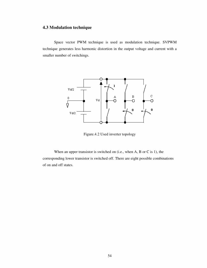
54

4.3 Modulation technique

Space vector PWM technique is used as modulation technique. SVPWM

technique generates less harmonic distortion in the output voltage and current with a

smaller number of switchings.

Figure.4.2 Used inverter topology When an upper transistor is switched on (i.e., when A, B or C is 1), the

corresponding lower transistor is switched off. There are eight possible combinations

of on and off states.

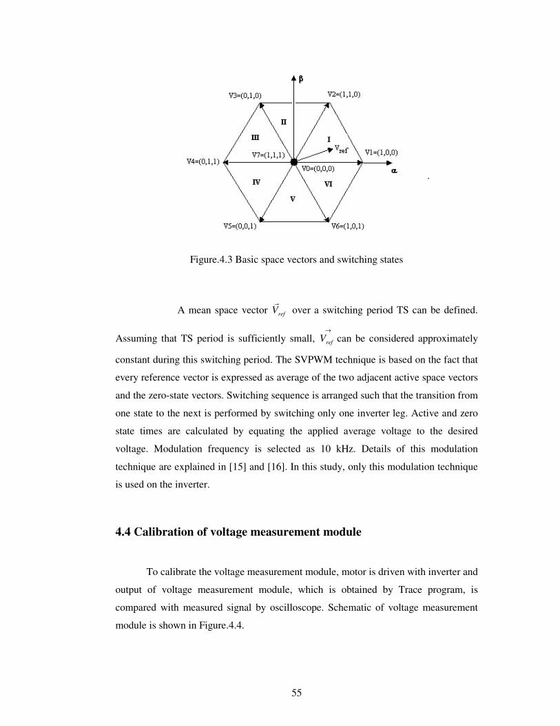
55

Figure.4.3 Basic space vectors and switching states

A mean space vector refV�

over a switching period TS can be defined.

Assuming that TS period is sufficiently small, →

refV can be considered approximately

constant during this switching period. The SVPWM technique is based on the fact that

every reference vector is expressed as average of the two adjacent active space vectors

and the zero-state vectors. Switching sequence is arranged such that the transition from

one state to the next is performed by switching only one inverter leg. Active and zero

state times are calculated by equating the applied average voltage to the desired

voltage. Modulation frequency is selected as 10 kHz. Details of this modulation

technique are explained in [15] and [16]. In this study, only this modulation technique

is used on the inverter.

4.4 Calibration of voltage measurement module

To calibrate the voltage measurement module, motor is driven with inverter and

output of voltage measurement module, which is obtained by Trace program, is

compared with measured signal by oscilloscope. Schematic of voltage measurement

module is shown in Figure.4.4.

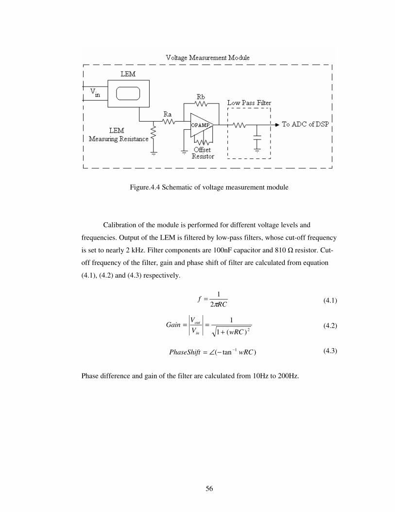
56

RCf

π21=

2)(1

1

wRCVV

Gainin

out

+==

)tan( 1 wRCPhaseShift −−∠=

Figure.4.4 Schematic of voltage measurement module

Calibration of the module is performed for different voltage levels and

frequencies. Output of the LEM is filtered by low-pass filters, whose cut-off frequency

is set to nearly 2 kHz. Filter components are 100nF capacitor and 810 � resistor. Cut-

off frequency of the filter, gain and phase shift of filter are calculated from equation

(4.1), (4.2) and (4.3) respectively.

(4.1)

(4.2)

(4.3)

Phase difference and gain of the filter are calculated from 10Hz to 200Hz.

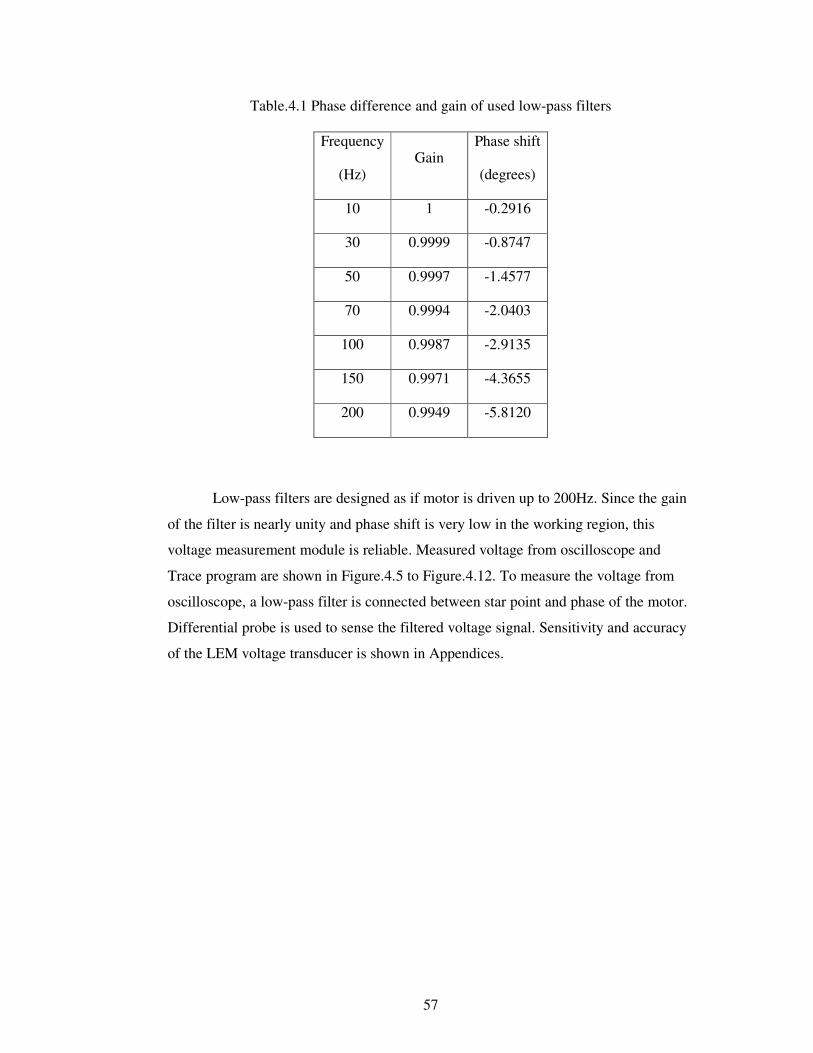
57

Table.4.1 Phase difference and gain of used low-pass filters

Frequency

(Hz) Gain

Phase shift

(degrees)

10 1 -0.2916

30 0.9999 -0.8747

50 0.9997 -1.4577

70 0.9994 -2.0403

100 0.9987 -2.9135

150 0.9971 -4.3655

200 0.9949 -5.8120

Low-pass filters are designed as if motor is driven up to 200Hz. Since the gain

of the filter is nearly unity and phase shift is very low in the working region, this

voltage measurement module is reliable. Measured voltage from oscilloscope and

Trace program are shown in Figure.4.5 to Figure.4.12. To measure the voltage from

oscilloscope, a low-pass filter is connected between star point and phase of the motor.

Differential probe is used to sense the filtered voltage signal. Sensitivity and accuracy

of the LEM voltage transducer is shown in Appendices.

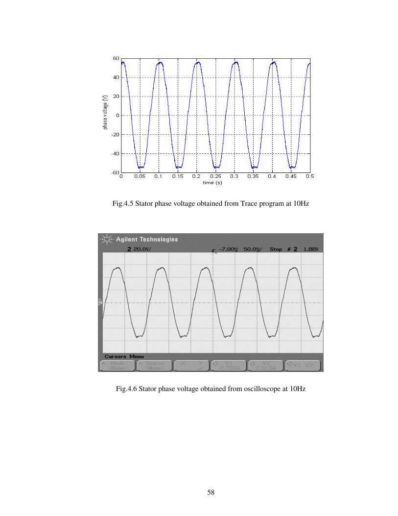
58

Fig.4.5 Stator phase voltage obtained from Trace program at 10Hz

Fig.4.6 Stator phase voltage obtained from oscilloscope at 10Hz

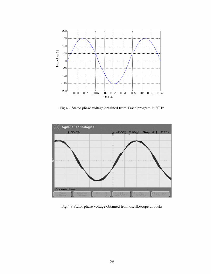
59

Fig.4.7 Stator phase voltage obtained from Trace program at 30Hz

Fig.4.8 Stator phase voltage obtained from oscilloscope at 30Hz

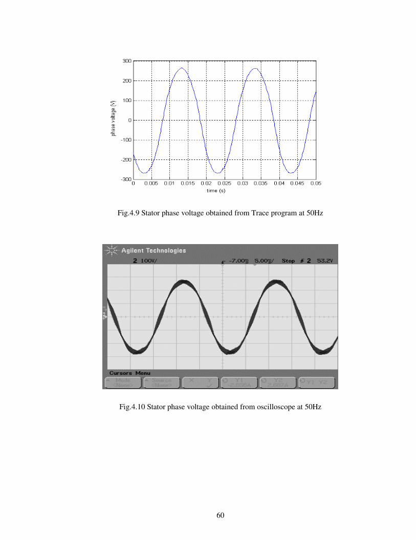
60

Fig.4.9 Stator phase voltage obtained from Trace program at 50Hz

Fig.4.10 Stator phase voltage obtained from oscilloscope at 50Hz

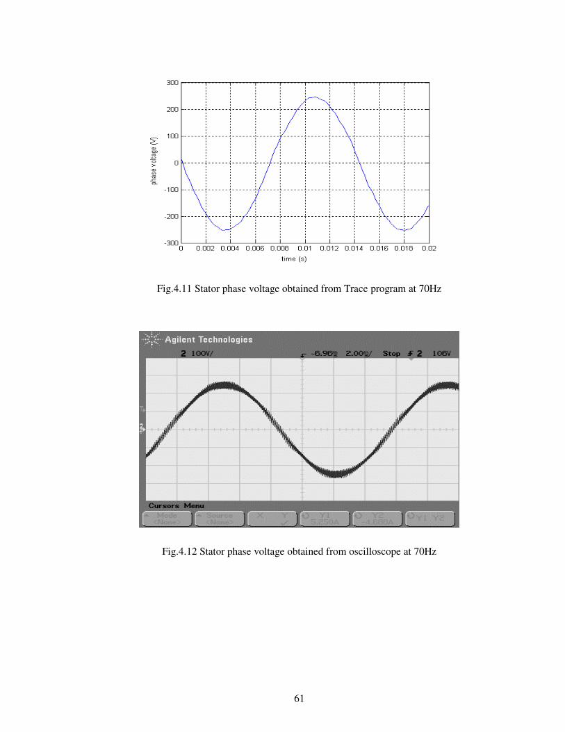
61

Fig.4.11 Stator phase voltage obtained from Trace program at 70Hz

Fig.4.12 Stator phase voltage obtained from oscilloscope at 70Hz

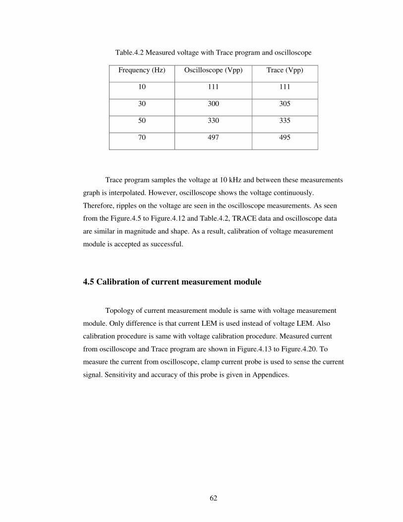
62

Table.4.2 Measured voltage with Trace program and oscilloscope

Frequency (Hz) Oscilloscope (Vpp) Trace (Vpp)

10 111 111

30 300 305

50 330 335

70 497 495

Trace program samples the voltage at 10 kHz and between these measurements

graph is interpolated. However, oscilloscope shows the voltage continuously.

Therefore, ripples on the voltage are seen in the oscilloscope measurements. As seen

from the Figure.4.5 to Figure.4.12 and Table.4.2, TRACE data and oscilloscope data

are similar in magnitude and shape. As a result, calibration of voltage measurement

module is accepted as successful.

4.5 Calibration of current measurement module

Topology of current measurement module is same with voltage measurement

module. Only difference is that current LEM is used instead of voltage LEM. Also

calibration procedure is same with voltage calibration procedure. Measured current

from oscilloscope and Trace program are shown in Figure.4.13 to Figure.4.20. To

measure the current from oscilloscope, clamp current probe is used to sense the current

signal. Sensitivity and accuracy of this probe is given in Appendices.

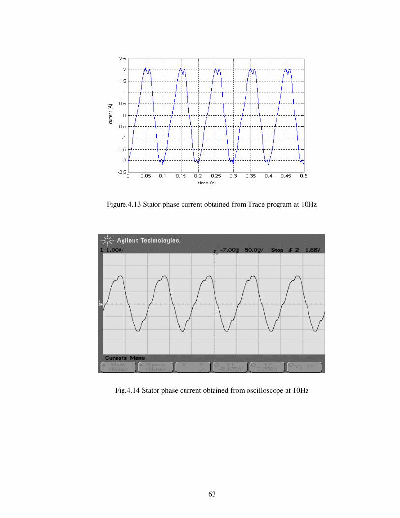
63

Figure.4.13 Stator phase current obtained from Trace program at 10Hz

Fig.4.14 Stator phase current obtained from oscilloscope at 10Hz

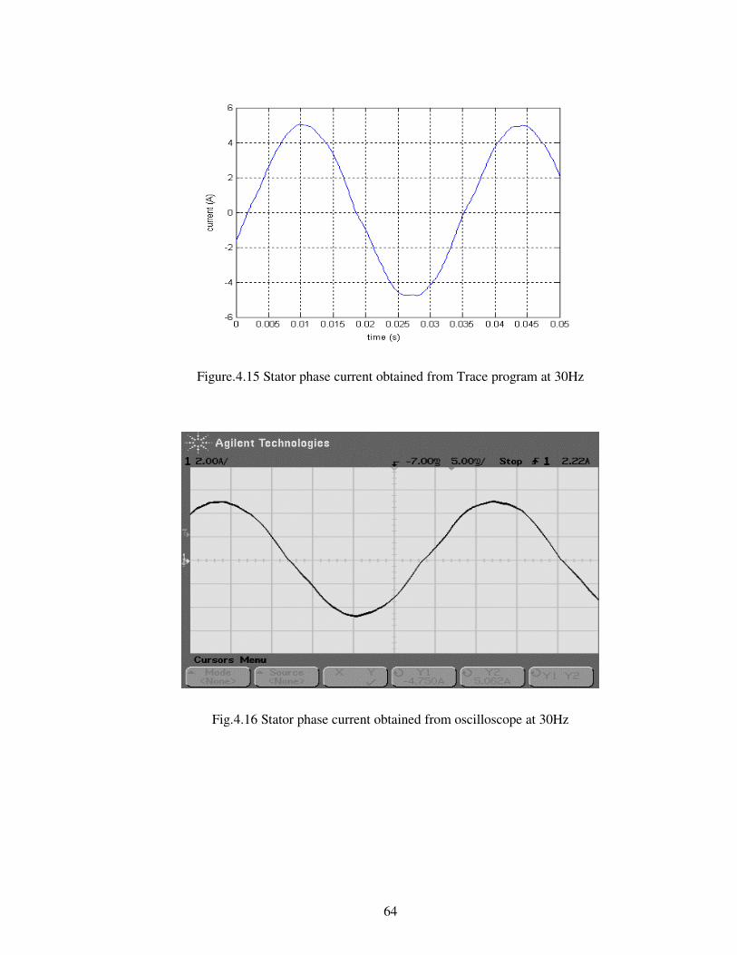
64

Figure.4.15 Stator phase current obtained from Trace program at 30Hz

Fig.4.16 Stator phase current obtained from oscilloscope at 30Hz

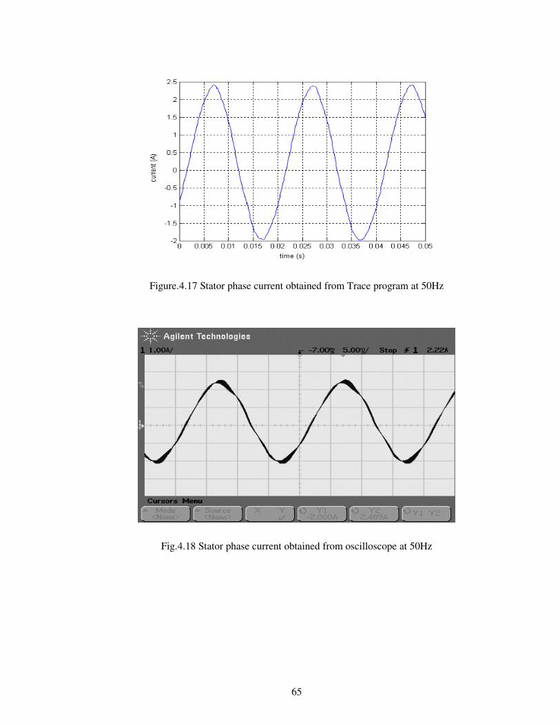
65

Figure.4.17 Stator phase current obtained from Trace program at 50Hz

Fig.4.18 Stator phase current obtained from oscilloscope at 50Hz

66

Figure.4.19 Stator phase current obtained from Trace program at 70Hz

Fig.4.20 Stator phase current obtained from oscilloscope at 70Hz

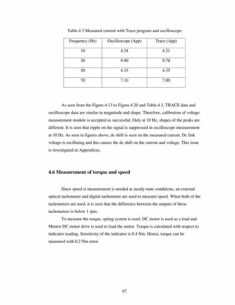
67

Table.4.3 Measured current with Trace program and oscilloscope

Frequency (Hz) Oscilloscope (App) Trace (App)

10 4.34 4.21

30 9.90 9.78

50 4.33 4.35

70 7.10 7.00

As seen from the Figure.4.13 to Figure.4.20 and Table.4.3, TRACE data and

oscilloscope data are similar in magnitude and shape. Therefore, calibration of voltage

measurement module is accepted as successful. Only at 10 Hz, shapes of the peaks are

different. It is seen that ripple on the signal is suppressed in oscilloscope measurement

at 10 Hz. As seen in figures above, dc shift is seen on the measured current. Dc link

voltage is oscillating and this causes the dc shift on the current and voltage. This issue

is investigated in Appendices.

4.6 Measurement of torque and speed

Since speed is measurement is needed at steady-state conditions, an external

optical tachometer and digital tachometer are used to measure speed. When both of the

tachometers are used, it is seen that the difference between the outputs of these

tachometers is below 1 rpm.

To measure the torque, spring system is used. DC motor is used as a load and

Mentor DC motor drive is used to load the motor. Torque is calculated with respect to

indicator reading. Sensitivity of the indicator is 0.4 Nm. Hence, torque can be

measured with 0.2 Nm error.

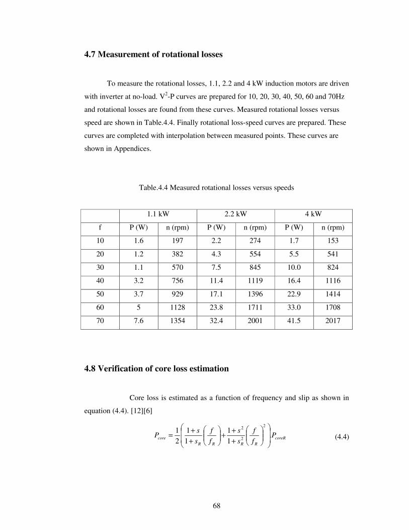
68

coreRRRRR

core Pff

ss

ff

ss

P .11

11

21

2

2

2

��

�

�

��

�

�

���

����

�

+++��

�

����

�

++=

4.7 Measurement of rotational losses

To measure the rotational losses, 1.1, 2.2 and 4 kW induction motors are driven

with inverter at no-load. V2-P curves are prepared for 10, 20, 30, 40, 50, 60 and 70Hz

and rotational losses are found from these curves. Measured rotational losses versus

speed are shown in Table.4.4. Finally rotational loss-speed curves are prepared. These

curves are completed with interpolation between measured points. These curves are

shown in Appendices.

Table.4.4 Measured rotational losses versus speeds

1.1 kW 2.2 kW 4 kW

f P (W) n (rpm) P (W) n (rpm) P (W) n (rpm)

10 1.6 197 2.2 274 1.7 153

20 1.2 382 4.3 554 5.5 541

30 1.1 570 7.5 845 10.0 824

40 3.2 756 11.4 1119 16.4 1116

50 3.7 929 17.1 1396 22.9 1414

60 5 1128 23.8 1711 33.0 1708

70 7.6 1354 32.4 2001 41.5 2017

4.8 Verification of core loss estimation

Core loss is estimated as a function of frequency and slip as shown in

equation (4.4). [12][6]

(4.4)

69

agsclincore PPPP −−=

where coreRP denotes core loss at rated condition, Rs slip at rated condition, Rf denotes

rated frequency, s denotes slip, f denotes frequency and coreP denotes core loss. This

equation is valid where flux linkage is kept constant at rated value. To verify this

estimation, core loss is measured and compared with estimated value. 2.2 kW induction

motor is driven from the mains (f=50Hz) under different load conditions and core loss

is calculated from measurement as shown in equation (4.5).

(4.5) where Pin denotes input power, Pscl denotes stator copper loss and Pag denotes air-gap

power. When motor is driven with inverter, input power is calculated by subtracting the

conduction loss and switching losses from the dc link power. Details of calculation of

inverter losses are investigated in Appendices. Estimated and measured core loss

values are shown in Fig.4.21, Table.4.5 and Table.4.6 for 2.2 kW motor.

Table.4.5 Estimated and measured core loss values for mains driven (f=50Hz) 2.2kW induction motor

Torque (Nm)

Speed (rpm)

Measured core loss (W)

Estimated core loss (W)

Error (%)

14.72 1400 139.5 161.95 -13.9 11.12 1426 123.2 160.5 -30.3 6.32 1460 125.6 158.6 -26.3 3.12 1478 191.1 157.6 17.5 1.52 1490 200.8 157 21.8

Table.4.6 Estimated and measured core loss values 2.2kW induction motor when driven with inverter

Frequency

(Hz)

Torque

(Nm)

Speed

(rpm)

Measured core loss

(W)

Estimated core loss

(W)

Error (%)

10 14.7 199 17.5 24 -37.1

10 14.7 209 19.8 23.4 -18.2

10 14.7 219 22.4 23 -2.7

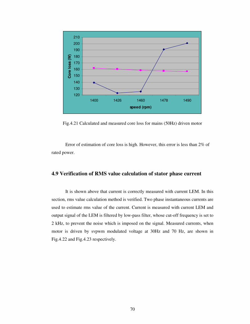
70

120

130

140

150

160

170

180

190

200

210

1400 1426 1460 1478 1490

speed (rpm)

Cor

e lo

ss (W

)

Fig.4.21 Calculated and measured core loss for mains (50Hz) driven motor Error of estimation of core loss is high. However, this error is less than 2% of

rated power.

4.9 Verification of RMS value calculation of stator phase current

It is shown above that current is correctly measured with current LEM. In this

section, rms value calculation method is verified. Two phase instantaneous currents are

used to estimate rms value of the current. Current is measured with current LEM and

output signal of the LEM is filtered by low-pass filter, whose cut-off frequency is set to

2 kHz, to prevent the noise which is imposed on the signal. Measured currents, when

motor is driven by svpwm modulated voltage at 30Hz and 70 Hz, are shown in

Fig.4.22 and Fig.4.23 respectively.

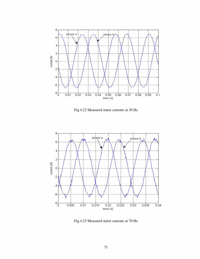
71

Fig.4.22 Measured stator currents at 30 Hz

Fig.4.23 Measured stator currents at 70 Hz

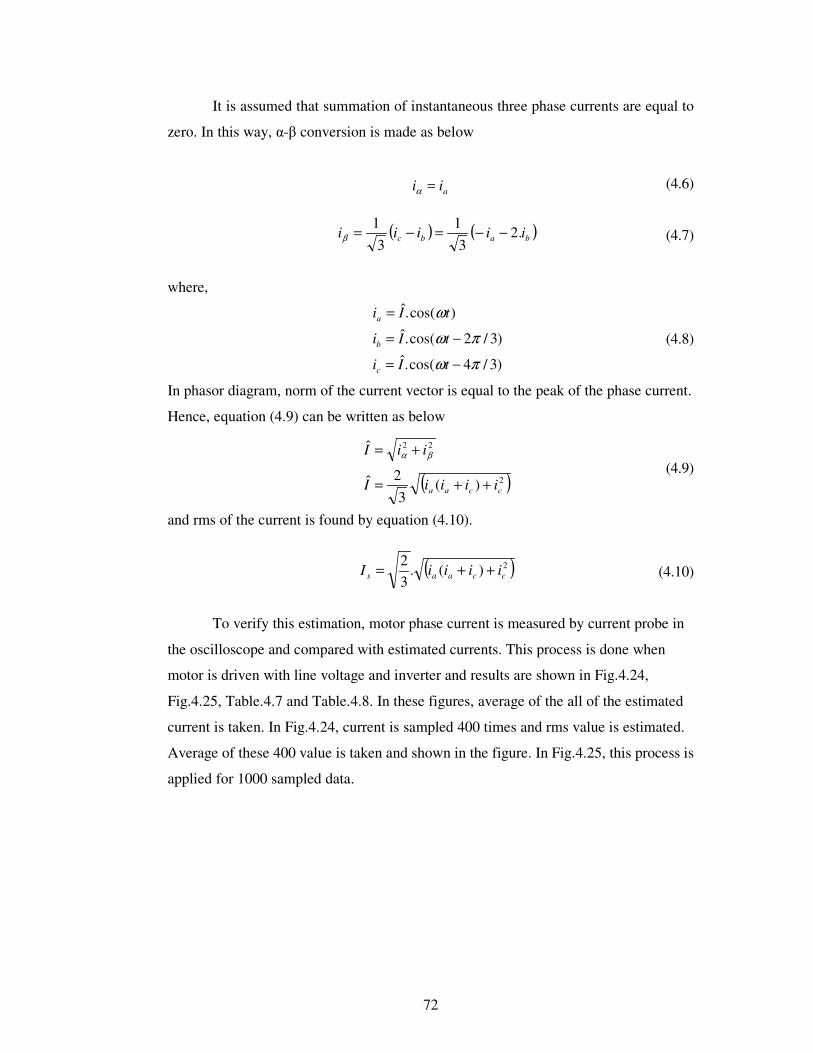
72

aii =α

( ) ( )babc iiiii .23

13

1 −−=−=β

)3/4cos(.ˆ)3/2cos(.ˆ

)cos(.ˆ

πω

πω

ω

−=

−=

=

tIi

tIi

tIi

c

b

a

( )2

22

)(3

2ˆ

ˆ

ccaa iiiiI

iiI

++=

+= βα

( )2)(.32

ccaas iiiiI ++=

It is assumed that summation of instantaneous three phase currents are equal to

zero. In this way, -� conversion is made as below

(4.6)

(4.7)

where,

(4.8)

In phasor diagram, norm of the current vector is equal to the peak of the phase current.

Hence, equation (4.9) can be written as below

(4.9)

and rms of the current is found by equation (4.10).

(4.10)

To verify this estimation, motor phase current is measured by current probe in

the oscilloscope and compared with estimated currents. This process is done when

motor is driven with line voltage and inverter and results are shown in Fig.4.24,

Fig.4.25, Table.4.7 and Table.4.8. In these figures, average of the all of the estimated

current is taken. In Fig.4.24, current is sampled 400 times and rms value is estimated.

Average of these 400 value is taken and shown in the figure. In Fig.4.25, this process is

applied for 1000 sampled data.

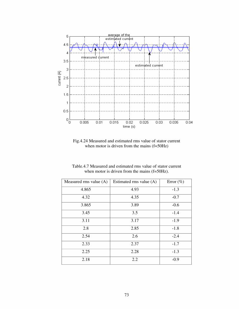
73

Fig.4.24 Measured and estimated rms value of stator current when motor is driven from the mains (f=50Hz)

Table.4.7 Measured and estimated rms value of stator current when motor is driven from the mains (f=50Hz).

Measured rms value (A) Estimated rms value (A) Error (%)

4.865 4.93 -1.3

4.32 4.35 -0.7

3.865 3.89 -0.6

3.45 3.5 -1.4

3.11 3.17 -1.9

2.8 2.85 -1.8

2.54 2.6 -2.4

2.33 2.37 -1.7

2.25 2.28 -1.3

2.18 2.2 -0.9

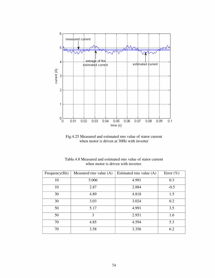
74

Fig.4.25 Measured and estimated rms value of stator current when motor is driven at 30Hz with inverter

Table.4.8 Measured and estimated rms value of stator current when motor is driven with inverter.

Frequency(Hz) Measured rms value (A) Estimated rms value (A) Error (%)

10 5.006 4.991 0.3

10 2.87 2.884 -0.5

30 4.89 4.818 1.5

30 3.03 3.024 0.2

50 5.17 4.991 3.5

50 3 2.951 1.6

70 4.85 4.594 5.3

70 3.58 3.356 6.2

75

In Fig.4.24, estimated rms value is oscillating. Frequency of this oscillation is

300Hz. It is thought that dc link voltage is oscillating and frequency of the output

voltage of the uncontrolled rectifier is seen on estimated rms value of current. If larger

capacitances had been selected, oscillation on the current could be reduced. To verify

the effect of this oscillation on the speed estimation results, 2.2 kW induction motor is

driven with line voltage and results of the estimation methods are compared with

results of estimation methods when motor is driven with inverter. Result of this

comparison is shown in Chapter 5. In Fig.4.25, another disturbing signal is added to the

estimated rms value of current. Frequency of this signal is 30Hz which is same with

frequency of produced voltage. It is shown that estimated rms value of stator phase

current is very similar to the measured value except 70Hz. Because, noise imposed on

the measured signal at high frequencies increases the error.

4.10 Verification of RMS value calculation of stator phase to neutral

voltage

It is shown above that voltage is correctly measured with voltage LEM. In this

section, rms value calculation method is verified. Main principle of estimation rms

value of the phase to neutral voltage is same with estimation of rms value of stator

current. Phase voltage is measured with voltage LEM and measured signal is filtered

by a low pass filter whose cut-off frequency is set to 2 kHz. Measured voltages, when

motor is driven by svpwm modulated voltage at 30Hz and 70 Hz, are shown in

Fig.4.26 and Fig.4.27 respectively.

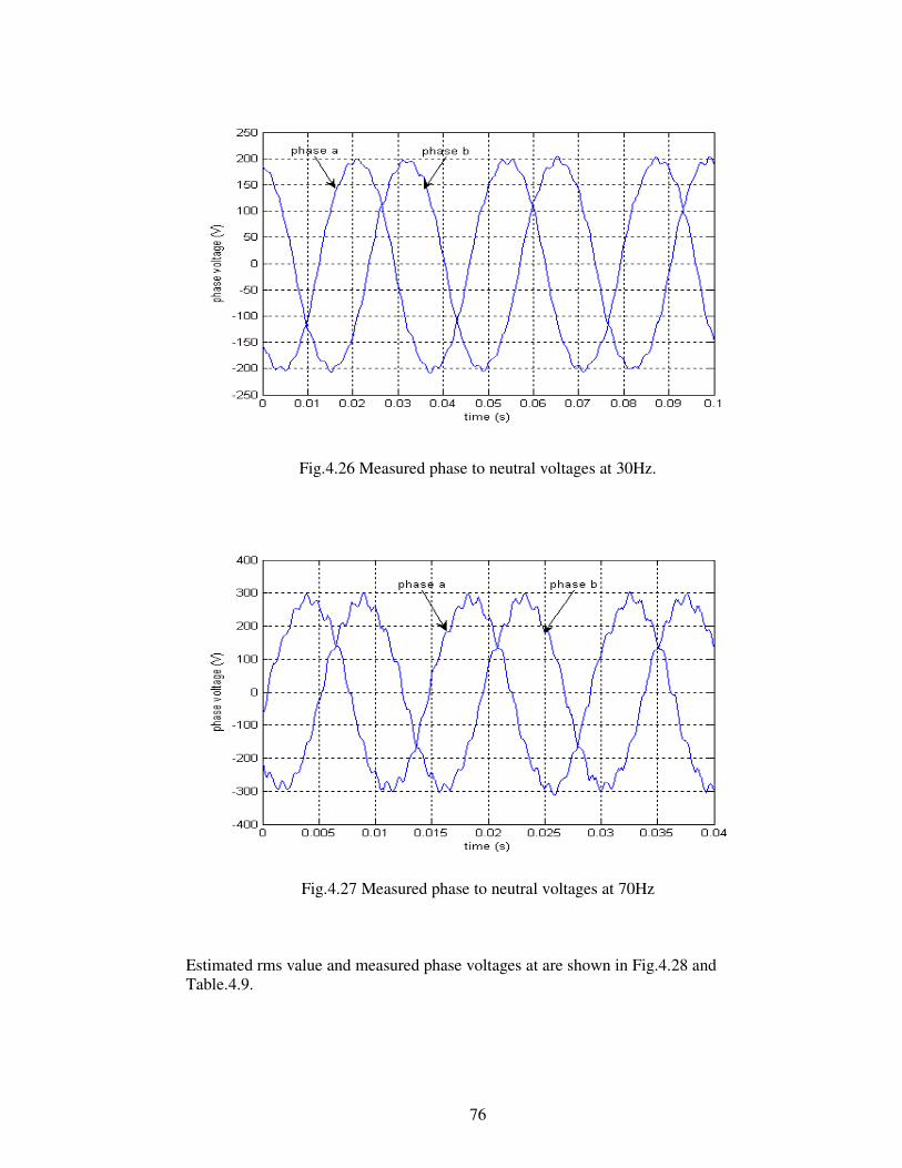
76

Fig.4.26 Measured phase to neutral voltages at 30Hz.

Fig.4.27 Measured phase to neutral voltages at 70Hz Estimated rms value and measured phase voltages at are shown in Fig.4.28 and Table.4.9.

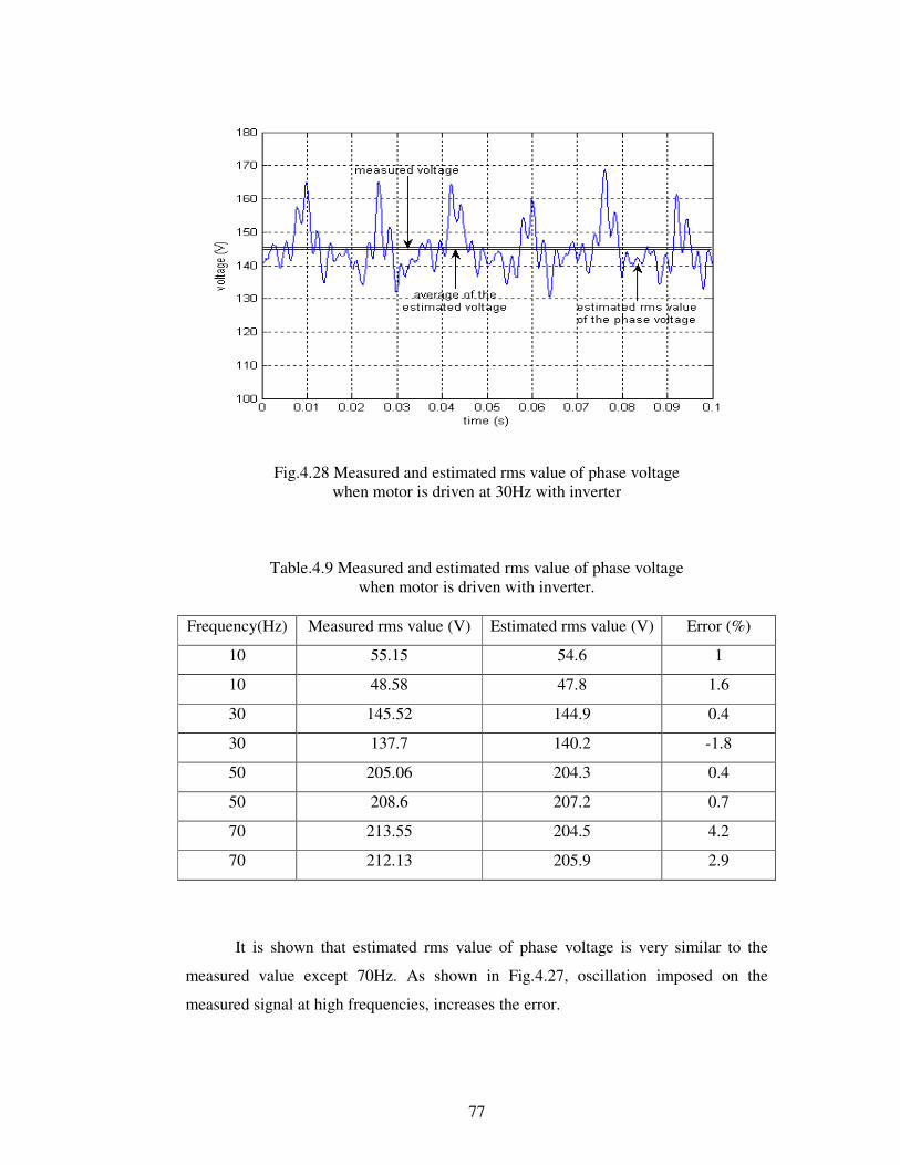
77

Fig.4.28 Measured and estimated rms value of phase voltage when motor is driven at 30Hz with inverter

Table.4.9 Measured and estimated rms value of phase voltage when motor is driven with inverter.

Frequency(Hz) Measured rms value (V) Estimated rms value (V) Error (%)

10 55.15 54.6 1

10 48.58 47.8 1.6

30 145.52 144.9 0.4

30 137.7 140.2 -1.8

50 205.06 204.3 0.4

50 208.6 207.2 0.7

70 213.55 204.5 4.2

70 212.13 205.9 2.9

It is shown that estimated rms value of phase voltage is very similar to the

measured value except 70Hz. As shown in Fig.4.27, oscillation imposed on the

measured signal at high frequencies, increases the error.

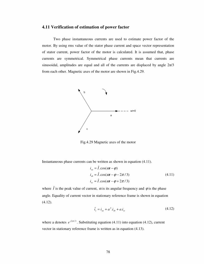
78

)3/2cos(.ˆ)3/2cos(.ˆ

)cos(.ˆ

πϕω

πϕω

ϕω

+−=

−−=

−=

tIi

tIi

tIi

sc

sb

sa

scsbsas iaiaii ..2 ++=�

4.11 Verification of estimation of power factor

Two phase instantaneous currents are used to estimate power factor of the

motor. By using rms value of the stator phase current and space vector representation

of stator current, power factor of the motor is calculated. It is assumed that, phase

currents are symmetrical. Symmetrical phase currents mean that currents are

sinusoidal, amplitudes are equal and all of the currents are displaced by angle 2�/3

from each other. Magnetic axes of the motor are shown in Fig.4.29.

Fig.4.29 Magnetic axes of the motor

Instantaneous phase currents can be written as shown in equation (4.11).

(4.11)

where I is the peak value of current, ω is its angular frequency and ϕ is the phase

angle. Equality of current vector in stationary reference frame is shown in equation

(4.12).

(4.12)

where a denotes 3/2πje . Substituting equation (4.11) into equation (4.12), current

vector in stationary reference frame is written as in equation (4.13).

79

)(.ˆ.23 ϕω −= tj

s eIi�

( )ϕϕϕ sin.cos.ˆ.23

.ˆ.23

jIeIi jes −== −�

{ }s

es

Ii�

Re.

32

cos =ϕ

tjes ejiii ω

βα )..(23 +=

�

{ } ( ))sin(.)cos(..23

Re titii es ωω βα −=�

lll

in

IVP

..3cos

−

=ϕ

(4.13)

In synchronous reference frame, current vector is written as equation (4.14).

(4.14)

Using equation (4.14), ϕcos (power factor) is written as equation (4.15)

(4.15)

Current vector in stationary reference frame is written as equation (4.16) and real part

of this vector is equal to the equation (4.17).

(4.16)

(4.17)

Substituting equation (4.10) and equation (4.17) into equation (4.15), power factor is

calculated.

To verify this estimation, 2.2kW induction motor is driven with line voltage and

inverter. When motor is driven with line voltage, HIOKI Power Meter is used to

measure input power, current and voltage.

(4.18)

Measured power factor, which is calculated from equation (4.18), is compared with

estimated current and results are shown in Table.4.10.

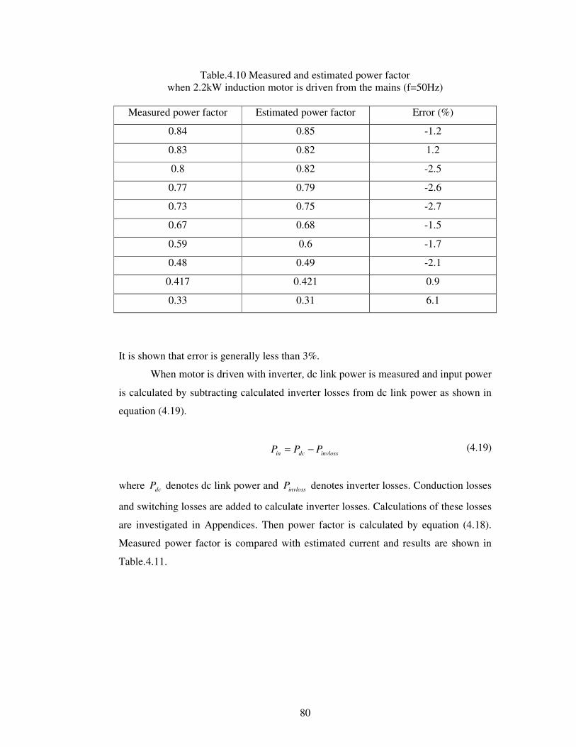
80

invlossdcin PPP −=

Table.4.10 Measured and estimated power factor when 2.2kW induction motor is driven from the mains (f=50Hz)

Measured power factor Estimated power factor Error (%)

0.84 0.85 -1.2

0.83 0.82 1.2

0.8 0.82 -2.5

0.77 0.79 -2.6

0.73 0.75 -2.7

0.67 0.68 -1.5

0.59 0.6 -1.7

0.48 0.49 -2.1

0.417 0.421 0.9

0.33 0.31 6.1

It is shown that error is generally less than 3%.

When motor is driven with inverter, dc link power is measured and input power

is calculated by subtracting calculated inverter losses from dc link power as shown in

equation (4.19).

(4.19)

where dcP denotes dc link power and invlossP denotes inverter losses. Conduction losses

and switching losses are added to calculate inverter losses. Calculations of these losses

are investigated in Appendices. Then power factor is calculated by equation (4.18).

Measured power factor is compared with estimated current and results are shown in

Table.4.11.

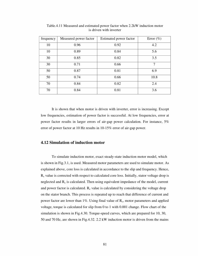
81

Table.4.11 Measured and estimated power factor when 2.2kW induction motor is driven with inverter

frequency Measured power factor Estimated power factor Error (%)

10 0.96 0.92 4.2

10 0.89 0.84 5.6

30 0.85 0.82 3.5

30 0.71 0.66 7

50 0.87 0.81 6.9

50 0.74 0.66 10.8

70 0.84 0.82 2.4

70 0.84 0.81 3.6

It is shown that when motor is driven with inverter, error is increasing. Except

low frequencies, estimation of power factor is successful. At low frequencies, error at

power factor results in larger errors of air-gap power calculation. For instance, 5%

error of power factor at 10 Hz results in 10-15% error of air-gap power.

4.12 Simulation of induction motor

To simulate induction motor, exact steady-state induction motor model, which

is shown in Fig.3.1, is used. Measured motor parameters are used to simulate motor. As

explained above, core loss is calculated in accordance to the slip and frequency. Hence,

Rc value is corrected with respect to calculated core loss. Initially, stator voltage drop is

neglected and Rc is calculated. Then using equivalent impedance of the model, current

and power factor is calculated. Rc value is calculated by considering the voltage drop

on the stator branch. This process is repeated up to reach that difference of current and

power factor are lower than 1%. Using final value of Rc, motor parameters and applied

voltage, torque is calculated for slip from 0 to 1 with 0.001 change. Flow chart of the

simulation is shown in Fig.4.30. Torque-speed curves, which are prepared for 10, 30,

50 and 70 Hz, are shown in Fig.4.32. 2.2 kW induction motor is driven from the mains

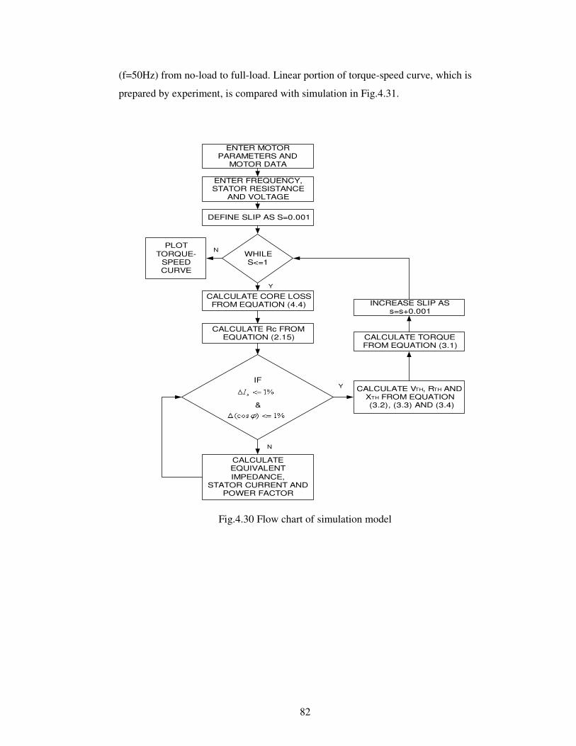
82

(f=50Hz) from no-load to full-load. Linear portion of torque-speed curve, which is

prepared by experiment, is compared with simulation in Fig.4.31.

ENTER MOTORPARAMETERS AND

MOTOR DATA

ENTER FREQUENCY,STATOR RESISTANCE

AND VOLTAGE

DEFINE SLIP AS S=0.001

WHILES<=1

CALCULATE CORE LOSSFROM EQUATION (4.4)

CALCULATE Rc FROMEQUATION (2.15)

IF

&

CALCULATEEQUIVALENTIMPEDANCE,

STATOR CURRENT ANDPOWER FACTOR

CALCULATE VTH, RTH ANDXTH FROM EQUATION(3.2), (3.3) AND (3.4)

CALCULATE TORQUEFROM EQUATION (3.1)

INCREASE SLIP ASs=s+0.001

Y

PLOTTORQUE-

SPEEDCURVE

N

N

Y

Fig.4.30 Flow chart of simulation model

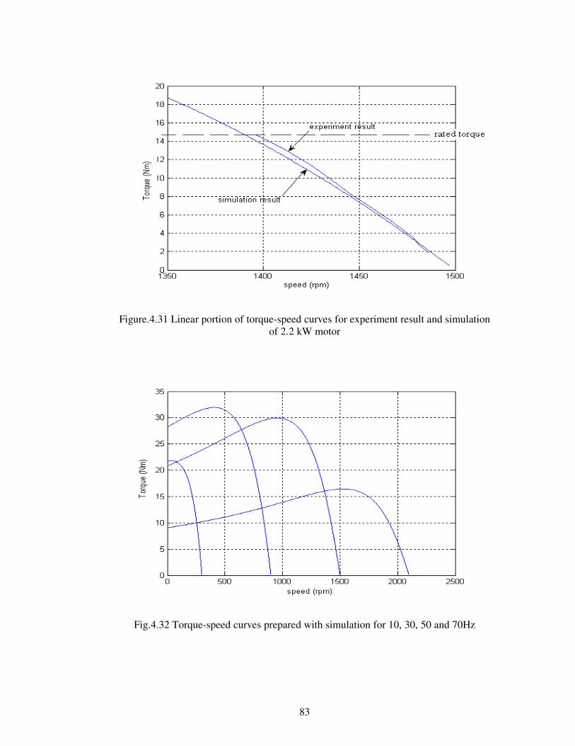
83

Figure.4.31 Linear portion of torque-speed curves for experiment result and simulation

of 2.2 kW motor

Fig.4.32 Torque-speed curves prepared with simulation for 10, 30, 50 and 70Hz

84

As seen from Fig.4.31, when load is increasing, difference between simulation

result and experiment result is increasing. Error of simulation is less than 10% for

50Hz. Motor model is verified in Chapter 5. Simulation codes are shown in

Appendices.

85

CHAPTER 5

VERIFICATION OF SPEED ESTIMATION METHODS

5.1 Introduction

In this chapter, results of the speed estimation methods presented in Chapter3

are investigated. Since the best accuracy of prediction may be expected when the exact

induction motor model is used, as explained in Chapter3, initially accuracy of the exact

induction motor model is investigated. Therefore, exact induction motor model is

simulated from 10Hz to70Hz and simulation results are compared with test results.

Then, accuracy of the speed estimation methods presented in Chapter 3 are

investigated. For comparison, results of speed estimation methods are compared with

simulation results from the exact induction motor model. This comparison shows the

relative accuracy of speed estimation methods with respect to the exact induction

motor model. Since the accuracy of the exact induction motor model is already

evaluated against tests, the most accurate method of prediction can be identified.

5.2 Verification of steady-state induction motor model

To verify the exact induction motor model shown in Fig.3.1, the induction

motor operation is simulated in Matlab environment and compared with test results.

The simulation software is described in Chapter 4. First one of the test motor (2.2 kW

induction motor) is driven from the mains and measured torque is compared with

simulation result as shown in Fig.4.31 and Table.5.1. Since electrical torque is

86

calculated in simulation, rotational loss is added to the load torque from measurements

to compare with simulation result.

Table.5.1 Measured torque and torque found from simulation of exact steady-state motor model for mains (50Hz) driven 2.2kW motor

Vs l-l

(V)

Speed

(rpm)

Measured torque

(Nm)

Torque from model

(Nm)

Error

(%)

380 1445 8.2 7.95 3.0

380 1396 14.6 13.8 5.5

As shown in Fig.4.31 and Table.5.1, torque-speed curves prepared by

simulation and tests for 2.2 kW induction motor are similar in shape. When speed is

taken as reference and torques from simulation and measurement are compared, 3%

error under half load and 6% error under full load are calculated. This is an acceptable

accuracy.

To investigate the effects of inverter pulsed waveform on the accuracy of exact

induction motor model, 2.2 kW induction motor is driven with inverter at 50 Hz and

test results are compared with simulation results.

Speed is taken as reference and torques from measurement and simulation are

compared. As shown in Table.5.3, error of the torque found from simulation is 4%

under half load and 14% under full load. It is observed that error in torque estimation is

increasing when motor is driven with inverter with respect to results obtained when

motor is driven from the mains.

When 2.2kW motor is driven with inverter at 50Hz, flux level is lower than

rated value since the dc link voltage does not permit higher voltage levels than applied.

Therefore, magnetizing reactance and core loss resistance is likely to be different from

the reference values obtained for rated flux. Furthermore, the pulsed waveform of the

inverter may affect the other parameters too. These may be the error sources. However,

this issue was not investigated further in this work.

To obtain the accuracy of the exact induction motor model when induction

motor is driven with inverter, 1.1kW, 2.2kW and 4kW induction motors are driven at

87

10Hz, 30Hz, 50Hz and 70Hz under half load and full load and test results are compared

with simulation results.

To produce maximum torque achievable for unit current, flux must be kept

constant at rated value for different loads when the motor is inverter driven. This is

especially important at low frequencies where the voltage drop on the series impedance

becomes comparable to applied voltage. Here however, during the tests the following

was done. The flux is in the +5% band of rated flux level for 1.1kW motor, in the

+10% band of the rated flux level for 2.2kW motor and in the -5% band of the rated

flux level for 4kW motor. During the tests the flux level was kept within the flux levels

defined above.

To make realistic predictions, measured voltages during the tests are selected as

input voltages of the simulations. Measured phase voltages are shown in Table.5.2,

Table.5.3 and Table.5.4. In these tables, measured torques and simulation results are

compared.

Table.5.2 Measured torque and torque found from simulation of exact steady-state motor model for 1.1kW motor

f

(Hz)

Vs

(V)

Speed

(rpm)

Measured torque

(Nm)

Torque from

model (Nm)

Error

(%)

10 50.9 136 5.3 6.8 -28.3

10 62.2 91 11.3 13.8 -22.1

30 129.4 550 5.2 6.2 -19.2

30 141.4 501 11.2 12.9 -15.2

50 219.2 954 5.2 6.4 -23.1

50 220.6 899 11.2 12.3 -9.8

70 220.6 1314 5.2 6.0 -15.4

70 220.6 1229 8.3 9.3 -12.0

88

Table.5.3 Measured torque and torque found from simulation of exact steady-state motor model for 2.2kW motor

f

(Hz)

Vs

(V)

Speed

(rpm)

Measured torque

(Nm)

Torque from

model (Nm)

Error

(%)

10 55.2 194 14.4 13.96 3.1

10 48.6 251 6.8 6.6 2.9

30 145.5 813 14.41 13.22 8.3

30 137.7 859 6.81 6.05 11.2

50 205.1 1384 14.41 12.4 14

50 208.6 1446 6.81 6.54 4

70 213.6 1943 10.21 8.97 12.1

70 212.1 1998 6.81 6.15 9.7

Table.5.4 Measured torque and torque found from simulation of exact steady-state motor model for 4kW motor

f

(Hz)

Vs

(V)

Speed

(rpm)

Measured torque

(Nm)

Torque from

model (Nm)

Error

(%)

10 70.6 250 13.5 12.6 6.7

10 85.9 218 26.7 25.0 6.4

30 212.5 861 13.5 12.3 8.9

30 229.2 829 26.7 23.6 11.6

50 351.7 1459 13.5 12.8 5.2

50 352.3 1424 26.8 21.8 18.7

70 351.8 2026 13.6 11.3 16.9

70 363.6 1970 22.0 19.0 13.6

In Table.5.2, Table.5.3 and Table.5.4, speed is taken as reference and measured

torque is compared with torque found from simulation of the exact induction motor

model. for 1.1kW motor, measured torque is smaller than the estimated torque and

error of the estimation is very high. Since rated torque of this motor is nearly 11Nm,

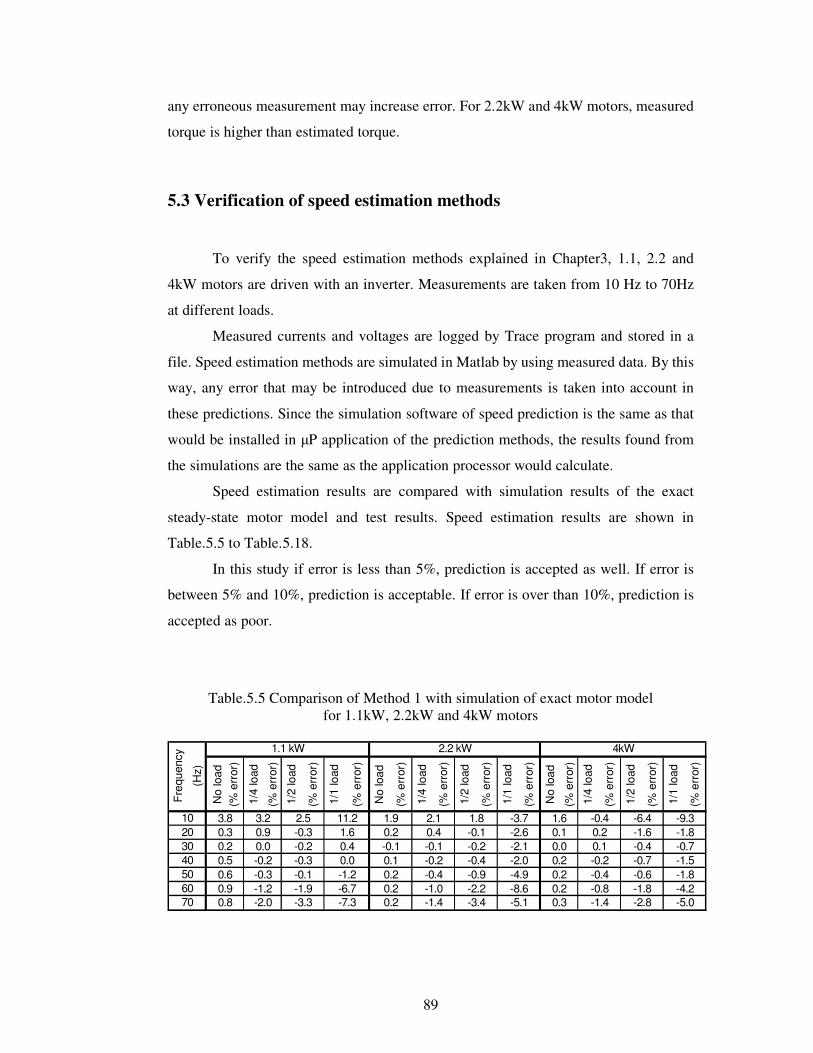
89

any erroneous measurement may increase error. For 2.2kW and 4kW motors, measured

torque is higher than estimated torque.

5.3 Verification of speed estimation methods

To verify the speed estimation methods explained in Chapter3, 1.1, 2.2 and

4kW motors are driven with an inverter. Measurements are taken from 10 Hz to 70Hz

at different loads.

Measured currents and voltages are logged by Trace program and stored in a

file. Speed estimation methods are simulated in Matlab by using measured data. By this

way, any error that may be introduced due to measurements is taken into account in

these predictions. Since the simulation software of speed prediction is the same as that

would be installed in �P application of the prediction methods, the results found from

the simulations are the same as the application processor would calculate.

Speed estimation results are compared with simulation results of the exact

steady-state motor model and test results. Speed estimation results are shown in

Table.5.5 to Table.5.18.

In this study if error is less than 5%, prediction is accepted as well. If error is

between 5% and 10%, prediction is acceptable. If error is over than 10%, prediction is

accepted as poor.

Table.5.5 Comparison of Method 1 with simulation of exact motor model for 1.1kW, 2.2kW and 4kW motors

No

load

(%

err

or)

1/4

load

(% e

rror

)

1/2

load

(% e

rror

)

1/1

load

(% e

rror

)

No

load

(% e

rror

)

1/4

load

(% e

rror

)

1/2

load

(% e

rror

)

1/1

load

(% e

rror

)

No

load

(% e

rror

)

1/4

load

(% e

rror

)

1/2

load

(% e

rror

)

1/1

load

(% e

rror

)

0.21.9

-6.7-1.2

1.611.2

0.20.20.20.1

0.00.93.2 2.5

-0.3

-1.9-0.1-0.3-0.2

-2.0-1.2-0.3-0.2

1.1 kW 4kW2.2 kW

-1.4-1.0-0.4-0.2-0.10.42.1

Fre

quen

cy

(Hz)

70

50

30

10

60

40

20

0.8

3.80.3

0.60.50.2

0.9-3.3

-2.6-3.7

-5.1-8.6-4.9-2.0-0.4

-0.2-0.1 0.1

1.6

-7.3 0.30.20.20.2

-2.1

1.8

-3.4-0.8-0.4

0.4-0.20.10.0

-2.2-0.9

-0.10.0

0.2-0.4

-2.8-1.8-0.6-0.7-0.4-1.6-6.4

-1.4

-0.7-1.8-9.3

-5.0-4.2-1.8-1.5

90

Table.5.6 Comparison of Method 1 with test result for 1.1kW, 2.2kW and 4kW motors

No

load

(%

err

or)

1/4

load

(% e

rror

)

1/2

load

(% e

rror

)

1/1

load

(% e

rror

)

No

load

(% e

rror

)

1/4

load

(% e

rror

)

1/2

load

(% e

rror

)

1/1

load

(% e

rror

)

No

load

(% e

rror

)

1/4

load

(% e

rror

)

1/2

load

(% e

rror

)

1/1

load

(% e

rror

)

-0.6-0.1-0.9-5.1

-0.6-2.7-3.9-2.1

-1.3-0.6

-6.2-0.40.2-0.5-0.3

-0.30.01.9

-0.9-1.2-1.60.1

0.0-0.3

1.1 kW 4kW2.2 kW

-3.4-2.3-1.3-0.7

-0.3-0.5-0.8

Freq

uenc

y

(Hz)

70

50

30

10

60

40

20

-1.5-3.1-7.5-5.1

-3.0-4.0-31.9 -8.7

-3.8-1.8-0.5

-0.6-3.8-0.4

0.0

-9.7-8.7-2.4-2.0

-1.1-1.6-2.30.7

0.50.2

-1.4-0.4-0.7-1.0

-0.20.13.8

-4.4-2.7-1.1-1.8-2.0-3.5-15.1 -0.4

0.20.0-0.4-0.7-0.8-1.20.2

0.0-0.3-0.1-0.10.11.6

Evaluation of Method 1 is given below.

a)low frequency:

- small motors: Poor performance is expected. The results found indicate that

performance of Method 1 is poor under full load condition. For other load conditions,

performance is good.

- medium motors: The results found indicate that performance of Method 1 is good for

all load conditions.

- large motors: Good performance is expected. The results found indicate that

performance of Method 1 is not good under full load condition. For other load

conditions, performance is good.

b)medium frequency:

- small motors: Good performance is expected. The results found indicate that

performance of Method 1 is good for all load conditions.

- medium motors: The results found indicate that performance of Method 1 is good for

all load conditions.

- large motors: Good performance is expected. The results found indicate that

performance of Method 1 is good for all load conditions.

c)high frequency:

- small motors: Poor performance is expected. The results found indicate that

performance of Method 1 is poor under full load condition. For other load conditions,

performance is good.

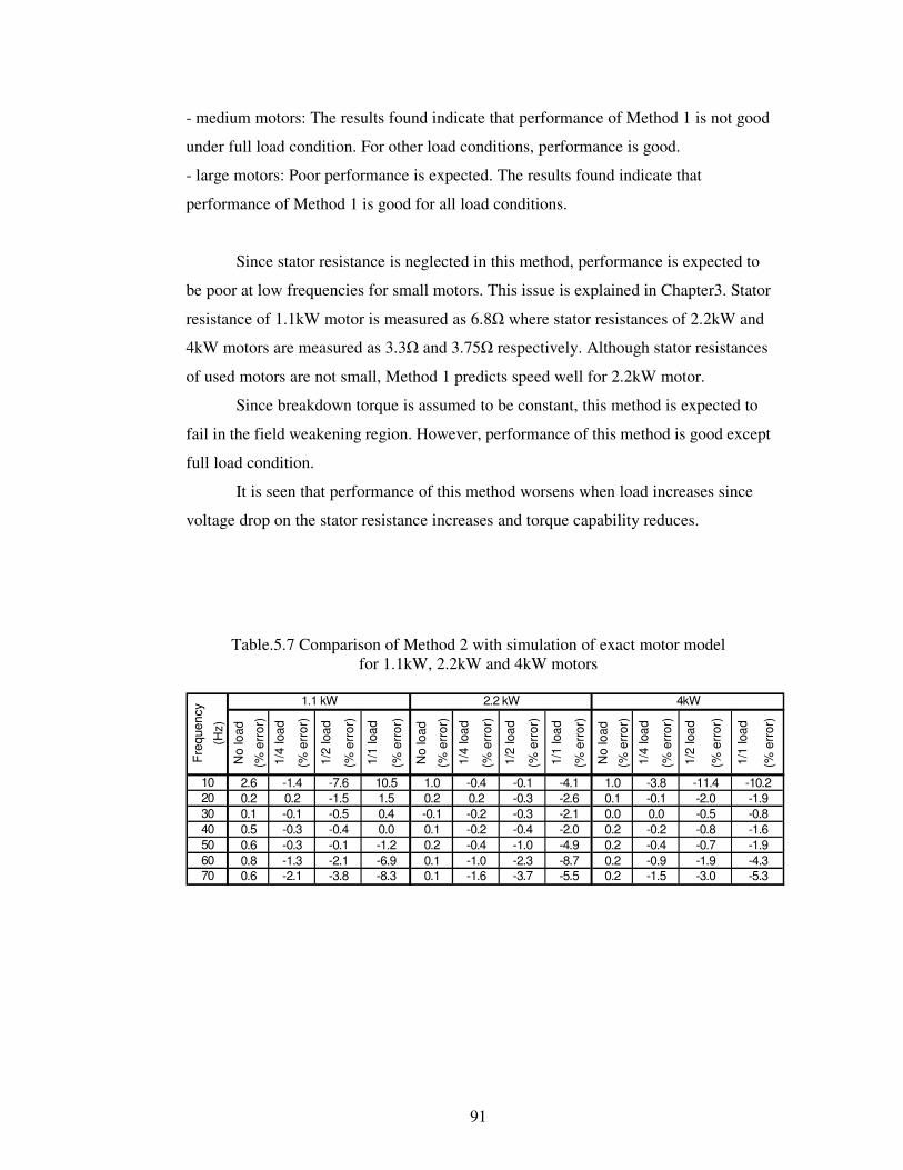
91

- medium motors: The results found indicate that performance of Method 1 is not good

under full load condition. For other load conditions, performance is good.

- large motors: Poor performance is expected. The results found indicate that

performance of Method 1 is good for all load conditions.

Since stator resistance is neglected in this method, performance is expected to

be poor at low frequencies for small motors. This issue is explained in Chapter3. Stator

resistance of 1.1kW motor is measured as 6.8� where stator resistances of 2.2kW and

4kW motors are measured as 3.3� and 3.75� respectively. Although stator resistances

of used motors are not small, Method 1 predicts speed well for 2.2kW motor.

Since breakdown torque is assumed to be constant, this method is expected to

fail in the field weakening region. However, performance of this method is good except

full load condition.

It is seen that performance of this method worsens when load increases since

voltage drop on the stator resistance increases and torque capability reduces.

Table.5.7 Comparison of Method 2 with simulation of exact motor model for 1.1kW, 2.2kW and 4kW motors

No

load

(% e

rror

)

1/4

load

(% e

rror

)

1/2

load

(% e

rror

)

1/1

load

(% e

rror

)

No

load

(% e

rror

)

1/4

load

(% e

rror

)

1/2

load

(% e

rror

)

1/1

load

(% e

rror

)

No

load

(% e

rror

)

1/4

load

(% e

rror

)

1/2

load

(% e

rror

)

1/1

load

(% e

rror

)

0.00.11.0

0.20.20.20.2

-0.5-2.0-11.4

-1.5-0.9-0.4-0.20.0-0.1-3.8

-3.0-1.9-0.7-0.8

-0.20.2-0.4

-5.3-4.3-1.9-1.6-0.8-1.9-10.2

-1.6-1.0-0.4-0.2

-2.1-2.6-4.1

-3.7-2.3-1.0-0.4-0.3-0.3-0.1

-5.5-8.7-4.9-2.0

0.41.510.5

0.10.10.20.1-0.10.21.0

-8.3-6.9-1.20.0

-0.10.2-1.4

-3.8-2.1-0.1-0.4-0.5-1.5-7.6

Fre

quen

cy

(Hz)

70

50

30

10

60

40

20

-2.1-1.3-0.3-0.3

1.1 kW 4kW2.2 kW

0.60.80.60.50.10.22.6

92

Table.5.8 Comparison of Method 2 with test result for 1.1kW, 2.2kW and 4kW motors

No

load

(%

err

or)

1/4

load

(% e

rror

)

1/2

load

(% e

rror

)

1/1

load

(% e

rror

)

No

load

(% e

rror

)

1/4

load

(% e

rror

)

1/2

load

(% e

rror

)

1/1

load

(% e

rror

)

No

load

(% e

rror

)

1/4

load

(% e

rror

)

1/2

load

(% e

rror

)

1/1

load

(% e

rror

)

-0.1

-8.9-2.4

-4.1

-2.9 0.0-0.3-0.2

-2.4-1.7-1.1-1.1

1.1 kW 4kW2.2 kW

-1.3-10.1-3.8

-0.10.11.0-32.8

Freq

uenc

y

(Hz)

70

50

30

10

60

40

20

0.5

-0.6-0.7-0.3-0.1

-0.4-0.7-0.8-1.40.1-4.9

-7.1-0.50.2-0.5-0.6-2.7-4.1-2.3

-1.4

0.01.0

-5.5-7.6-3.2-1.5-1.8-3.9-9.1

-3.0-2.0

0.10.0-0.3-0.3-0.3

-10.7

-0.5-0.9-5.8

-1.7-1.3-0.9-0.8-0.6-0.5-3.0

-3.8-2.4-1.4-0.7

0.40.20.0-0.20.02.6

-1.1-1.9-2.4-4.8-26.9-6.2

-1.1-0.8

Evaluation of Method 2 is given below.

a)low frequency:

- small motors: Poor performance is expected. The results found indicate that

performance of Method 2 is poor under full load and half load conditions. For other

load conditions, performance is good.

- medium motors: The results found indicate that performance of Method 2 is good for

all load conditions.

- large motors: Good performance is expected. The results found indicate that

performance of Method 2 is poor under full load and half load conditions. For other

load conditions, performance is good.

b)medium frequency:

- small motors: Good performance is expected. The results found indicate that

performance of Method 2 is good for all load conditions.

- medium motors: The results found indicate that performance of Method 2 is good for

all load conditions.

- large motors: Good performance is expected. The results found indicate that

performance of Method 2 is good for all load conditions.

c)high frequency:

- small motors: Good performance is expected. The results found indicate that

performance of Method 2 is not good under full load condition. For other load

conditions, performance is good.

93

- medium motors: The results found indicate that performance of Method 2 is not good

under full load condition. For other load conditions, performance is good.

- large motors: Good performance is expected. The results found indicate that

performance of Method 2 is not good under full load condition. For other load

conditions, performance is good.

This method is expected to improve the performance of Method 1 in the field

weakening region. However, results found indicate that performance of Method 2 is

worse than Method 1 in the field weakening region.

Table.5.9 Comparison of Method 3 with simulation of exact motor model for 1.1kW, 2.2kW and 4kW motors

No

load

(% e

rror

)

1/4

load

(% e

rror

)

1/2

load

(% e

rror

)

1/1

load

(% e

rror

)

No

load

(% e

rror

)

1/4

load

(% e

rror

)

1/2

load

(% e

rror

)

1/1

load

(% e

rror

)

No

load

(% e

rror

)

1/4

load

(% e

rror

)

1/2

load

(% e

rror

)

1/1

load

(% e

rror

)

1.1 kW 4kW2.2 kW

Fre

quen

cy

(Hz)

70

50

30

10

60

40

20

0.90.90.70.50.20.44.4

-1.9-1.1-0.10.00.41.86.2

-3.0-1.60.30.30.71.610.7

-6.9-6.0-0.31.43.07.537.3

-3.3-2.1-0.8-0.20.10.74.8

0.20.20.20.1-0.10.22.0

-1.4-0.9-0.3-0.10.00.73.2

-4.9-8.3-4.6-1.5-1.2-0.64.7

0.30.30.20.20.00.21.7

-1.4-0.8-0.3-0.10.20.40.4

-2.7-1.7-0.5-0.5-0.1-1.0-4.1

-4.9-4.0-1.6-1.20.00.0-1.7

Table.5.10 Comparison of Method 3 with test result for 1.1kW, 2.2kW and 4kW motors

No

load

(%

err

or)

1/4

load

(% e

rror

)

1/2

load

(% e

rror

)

1/1

load

(% e

rror

)

No

load

(% e

rror

)

1/4

load

(% e

rror

)

1/2

load

(% e

rror

)

1/1

load

(% e

rror

)

No

load

(% e

rror

)

1/4

load

(% e

rror

)

1/2

load

(% e

rror

)

1/1

load

(% e

rror

)

-1.2-1.50.1

0.0

0.0-0.3-0.7-0.8 -1.2

-0.5-0.10.1

-7.3-4.9-3.4

-2.2

-1.8-1.0-1.1-2.8

1.1 kW 4kW2.2 kW

0.1-0.60.72.0 1.1-2.80.4

Freq

uenc

y

(Hz)

70

50

30

10

60

40

20

0.0-0.10.14.4

-1.0-1.5-2.20.8

0.60.3

1.70.4-0.3-0.8 -1.2

-1.1-1.6-5.7

-1.5-8.0-9.3-4.1

-2.4-0.7

5.92.2-0.3-0.6

-0.3-0.3-0.30.1 1.3

1.0-0.1-0.4-2.5-3.8-2.0

-1.2-0.4-0.40.1-0.30.4

0.1-0.3-0.7-0.7-1.20.2

0.0

1.7

-0.3-0.1-0.10.2

94

Evaluation of Method 3 is given below.

a)low frequency:

- small motors: Poor performance is expected. The results found indicate that

performance of Method 3 is poor except no-load condition.

- medium motors: The results found indicate that performance of Method 3 is good for

all load conditions.

- large motors: Poor performance is expected. The results found indicate that

performance of Method 3 is good for all load conditions.

b)medium frequency:

- small motors: Good performance is expected. The results found indicate that

performance of Method 3 is good for all load conditions.

- medium motors: The results found indicate that performance of Method 3 is good for

all load conditions.

- large motors: Good performance is expected. The results found indicate that

performance of Method 3 is good for all load conditions.

c)high frequency:

- small motors: Poor performance is expected. The results found indicate that

performance of Method 3 is not good under full load condition. For other load

conditions, performance is good.

- medium motors: The results found indicate that performance of Method 3 is not good

under full load condition. For other load conditions, performance is good.

- large motors: Poor performance is expected. The results found indicate that

performance of Method 3 is good for all load conditions.

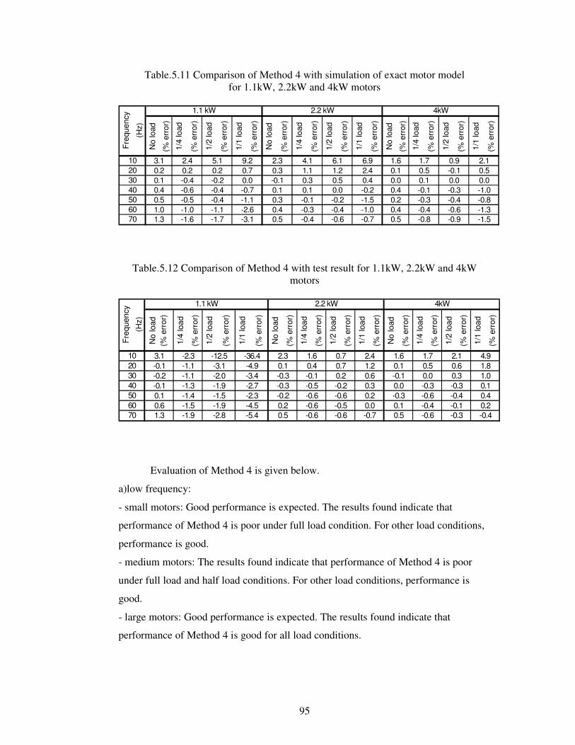
95

Table.5.11 Comparison of Method 4 with simulation of exact motor model for 1.1kW, 2.2kW and 4kW motors

No

load

(% e

rror

)

1/4

load

(% e

rror

)

1/2

load

(% e

rror

)

1/1

load

(% e

rror

)

No

load

(% e

rror

)

1/4

load

(% e

rror

)

1/2

load

(% e

rror

)

1/1

load

(% e

rror

)

No

load

(% e

rror

)

1/4

load

(% e

rror

)

1/2

load

(% e

rror

)

1/1

load

(% e

rror

)

70

50

30

10

60

40

20

1.1 kW 4kW2.2 kW

Freq

uenc

y

(Hz)

1.31.00.50.40.10.23.1

-1.6-1.0-0.5-0.6-0.40.22.4

-1.7-1.1-0.4-0.4-0.20.25.1

-3.1-2.6-1.1-0.70.00.79.2

0.50.40.30.1-0.10.32.3

-0.4-0.3-0.10.10.31.14.1

-0.6-0.4-0.20.00.51.26.1

-0.7-1.0-1.5-0.20.42.46.9

0.50.40.20.40.00.11.6

-0.8-0.4-0.3-0.10.10.51.7

-0.9-0.6-0.4-0.30.0-0.10.9

-1.5-1.3-0.8-1.00.00.52.1

Table.5.12 Comparison of Method 4 with test result for 1.1kW, 2.2kW and 4kW motors

No

load

(%

err

or)

1/4

load

(% e

rror

)

1/2

load

(% e

rror

)

1/1

load

(% e

rror

)

No

load

(% e

rror

)

1/4

load

(% e

rror

)

1/2

load

(% e

rror

)

1/1

load

(% e

rror

)

No

load

(% e

rror

)

1/4

load

(% e

rror

)

1/2

load

(% e

rror

)

1/1

load

(% e

rror

)

1.6

-4.5-2.3

-4.9-36.4

0.0-0.10.1

-1.1-1.1 -3.1

-1.9-1.5

0.0-0.3-0.6-0.4-0.60.5

0.1-0.3

1.1 kW 4kW2.2 kW

-0.4-0.30.30.62.11.7

0.5

Freq

uenc

y

(Hz)

70

50

30

10

60

40

20

1.3

4.91.81.00.10.40.2-0.4-0.3

-0.1-2.8

2.41.20.60.30.20.0-0.7

-1.9

-12.50.70.71.6

0.4-3.4-2.7

-0.6-0.5-0.6-0.20.2-0.1

-0.5

-5.4

-0.3-0.30.12.3

-0.6-0.6-0.60.5

0.2-0.2

0.60.1-0.1-0.2-0.13.1

-1.5-1.9-2.0

-1.3-1.4

-2.3

Evaluation of Method 4 is given below.

a)low frequency:

- small motors: Good performance is expected. The results found indicate that

performance of Method 4 is poor under full load condition. For other load conditions,

performance is good.

- medium motors: The results found indicate that performance of Method 4 is poor

under full load and half load conditions. For other load conditions, performance is

good.

- large motors: Good performance is expected. The results found indicate that

performance of Method 4 is good for all load conditions.

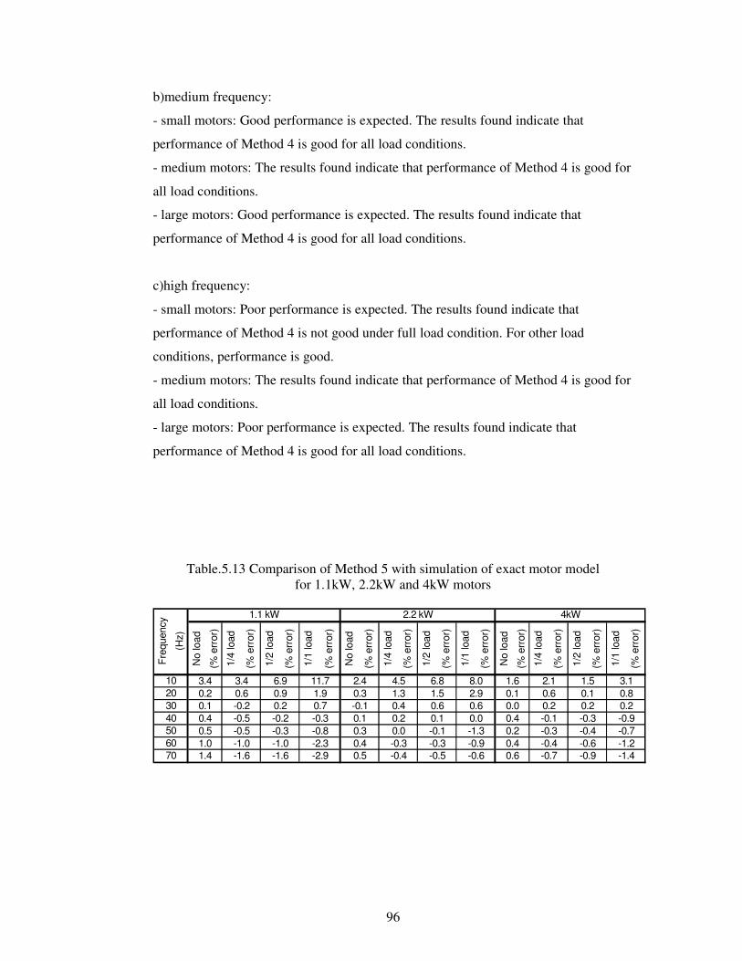
96

b)medium frequency:

- small motors: Good performance is expected. The results found indicate that

performance of Method 4 is good for all load conditions.

- medium motors: The results found indicate that performance of Method 4 is good for

all load conditions.

- large motors: Good performance is expected. The results found indicate that

performance of Method 4 is good for all load conditions.

c)high frequency:

- small motors: Poor performance is expected. The results found indicate that

performance of Method 4 is not good under full load condition. For other load

conditions, performance is good.

- medium motors: The results found indicate that performance of Method 4 is good for

all load conditions.

- large motors: Poor performance is expected. The results found indicate that

performance of Method 4 is good for all load conditions.

Table.5.13 Comparison of Method 5 with simulation of exact motor model for 1.1kW, 2.2kW and 4kW motors

No

load

(% e

rror

)

1/4

load

(% e

rror

)

1/2

load

(% e

rror

)

1/1

load

(% e

rror

)

No

load

(% e

rror

)

1/4

load

(% e

rror

)

1/2

load

(% e

rror

)

1/1

load

(% e

rror

)

No

load

(% e

rror

)

1/4

load

(% e

rror

)

1/2

load

(% e

rror

)

1/1

load

(% e

rror

)

70

50

30

10

60

40

20

1.1 kW 4kW2.2 kW

Freq

uenc

y

(Hz)

1.41.00.50.40.10.23.4

-1.6-1.0-0.5-0.5-0.20.63.4

-1.0-0.3

0.2-0.2

0.96.9

-2.9-2.3-0.8-0.30.71.911.7

-1.6 0.50.40.30.1-0.10.32.4

-0.5-0.3-0.10.10.61.56.8

-0.4-0.30.00.20.41.34.5

-0.6-0.9-1.30.00.62.98.0

-0.70.6-0.40.4

0.00.60.1

-0.30.2-0.10.4

2.11.6

-0.9-0.6-0.4-0.30.20.11.5

0.2 0.20.83.1

-1.4-1.2-0.7-0.9

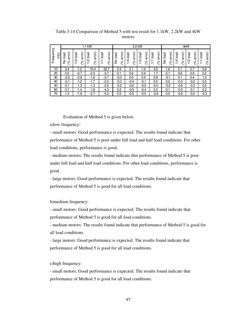
97

Table.5.14 Comparison of Method 5 with test result for 1.1kW, 2.2kW and 4kW motors

No

load

(%

err

or)

1/4

load

(% e

rror

)

1/2

load

(% e

rror

)

1/1

load

(% e

rror

)

No

load

(% e

rror

)

1/4

load

(% e

rror

)

1/2

load

(% e

rror

)

1/1

load

(% e

rror

)

No

load

(% e

rror

)

1/4

load

(% e

rror

)

1/2

load

(% e

rror

)

1/1

load

(% e

rror

)

-1.2 -10.4-2.3

-0.1-3.7-32.7

0.1-0.20.0

-0.9

-4.3-2.0

-1.9-1.4-1.3-1.2

1.1 kW 4kW2.2 kW

0.92.72.1

0.60.11.6

-0.7

Freq

uenc

y

(Hz)

70

50

30

10

60

40

20

1.3

-0.3-0.20.40.1

-0.3-0.6-0.3-0.60.5-2.7

5.82.21.20.20.50.3-0.3-0.2

-0.1-5.2

-0.5-0.4-0.5-0.5

-2.7-2.3

0.90.4-0.1

0.62.1

-0.60.20.40.50.91.73.51.4

-0.5-0.6-0.40.0

-1.7-1.6

0.70.1-0.1-0.2

-1.8

0.03.4

0.50.2-0.2-0.3-0.30.12.4

-1.3

Evaluation of Method 5 is given below.

a)low frequency:

- small motors: Good performance is expected. The results found indicate that

performance of Method 5 is poor under full load and half load conditions. For other

load conditions, performance is good.

- medium motors: The results found indicate that performance of Method 5 is poor

under full load and half load conditions. For other load conditions, performance is

good.

- large motors: Good performance is expected. The results found indicate that

performance of Method 5 is good for all load conditions.

b)medium frequency:

- small motors: Good performance is expected. The results found indicate that

performance of Method 5 is good for all load conditions.

- medium motors: The results found indicate that performance of Method 5 is good for

all load conditions.

- large motors: Good performance is expected. The results found indicate that

performance of Method 5 is good for all load conditions.

c)high frequency:

- small motors: Good performance is expected. The results found indicate that

performance of Method 5 is good for all load conditions.

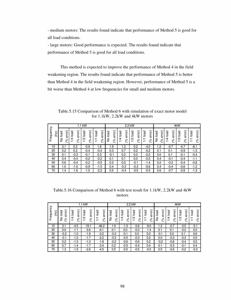
98

- medium motors: The results found indicate that performance of Method 5 is good for

all load conditions.

- large motors: Good performance is expected. The results found indicate that

performance of Method 5 is good for all load conditions.

This method is expected to improve the performance of Method 4 in the field

weakening region. The results found indicate that performance of Method 5 is better

than Method 4 in the field weakening region. However, performance of Method 5 is a

bit worse than Method 4 at low frequencies for small and medium motors.

Table.5.15 Comparison of Method 6 with simulation of exact motor model for 1.1kW, 2.2kW and 4kW motors

No

load

(% e

rror

)

1/4

load

(% e

rror

)

1/2

load

(% e

rror

)

1/1

load

(% e

rror

)

No

load

(% e

rror

)

1/4

load

(% e

rror

)

1/2

load

(% e

rror

)

1/1

load

(% e

rror

)

No

load

(% e

rror

)

1/4

load

(% e

rror

)

1/2

load

(% e

rror

)

1/1

load

(% e

rror

)

70

50

30

10

60

40

20

1.1 kW 4kW2.2 kW

Fre

quen

cy

(Hz)

1.41.00.60.40.10.23.1

-1.6-1.0-0.4-0.4-0.30.20.3

-0.2-0.1-0.4-0.9 1.6

-0.40.3-0.2-0.5-1.5-2.2-1.5

-0.9-0.2

0.50.40.30.1-0.10.31.9

-0.4-0.30.00.10.20.71.3 -4.0

-0.2-0.2-0.3-1.4-0.6-0.5-0.5

-0.3-0.10.00.20.20.2

-1.3-1.2-0.8-1.1-0.4-1.3-8.1-4.7

-0.9-0.1-0.4-0.4-0.6-0.8-0.7

-0.4-0.3-0.10.10.1-0.7

0.60.40.20.40.00.11.2

Table.5.16 Comparison of Method 6 with test result for 1.1kW, 2.2kW and 4kW motors

No

load

(%

err

or)

1/4

load

(% e

rror

)

1/2

load

(% e

rror

)

1/1

load

(% e

rror

)

No

load

(% e

rror

)

1/4

load

(% e

rror

)

1/2

load

(% e

rror

)

1/1

load

(% e

rror

)

No

load

(% e

rror

)

1/4

load

(% e

rror

)

1/2

load

(% e

rror

)

1/1

load

(% e

rror

)

-3.4-1.8

-6.1-46.2

-1.1-4.5 -19.1

-3.6

-1.9-1.4-1.3-1.2

1.1 kW 4kW2.2 kW

1.2

Fre

quen

cy

(Hz)

70

50

30

10

60

40

20

1.3

-0.2-3.5-0.7

0.1

0.1-0.20.0-0.10.1

-2.6

-0.4-0.30.10.0

-0.3-0.6-0.3-0.60.5-4.5

-5.10.00.60.00.50.4-0.2-0.2

-0.1

-3.2-2.2

-0.3-5.6-1.3

0.0-0.1-0.5

-0.4-0.6-0.30.0

-0.50.5

-9.0-1.40.00.20.20.4-0.5-0.5

-1.3-1.7-1.9

0.70.2-0.1-0.2

-1.7

-1.00.03.1

-0.6-0.50.2

-0.2-0.3-0.30.11.9

99

Evaluation of Method 6 is given below.

a)low frequency:

- small motors: Good performance is expected. The results found indicate that

performance of Method 6 is good for all load conditions.

- medium motors: The results found indicate that performance of Method 6 is good for

all load conditions.

- large motors: Good performance is expected. The results found indicate that

performance of Method 6 is not good under full load condition. For other load

conditions, performance is good.

b)medium frequency:

- small motors: Good performance is expected. The results found indicate that

performance of Method 6 is good for all load conditions.

- medium motors: The results found indicate that performance of Method 6 is good for

all load conditions.

- large motors: Good performance is expected. The results found indicate that

performance of Method 6 is good for all load conditions.

c)high frequency:

- small motors: Good performance is expected. The results found indicate that

performance of Method 6 is good for all load conditions.

- medium motors: The results found indicate that performance of Method 6 is good for

all load conditions.

- large motors: Good performance is expected. The results found indicate that

performance of Method 6 is good for all load conditions.

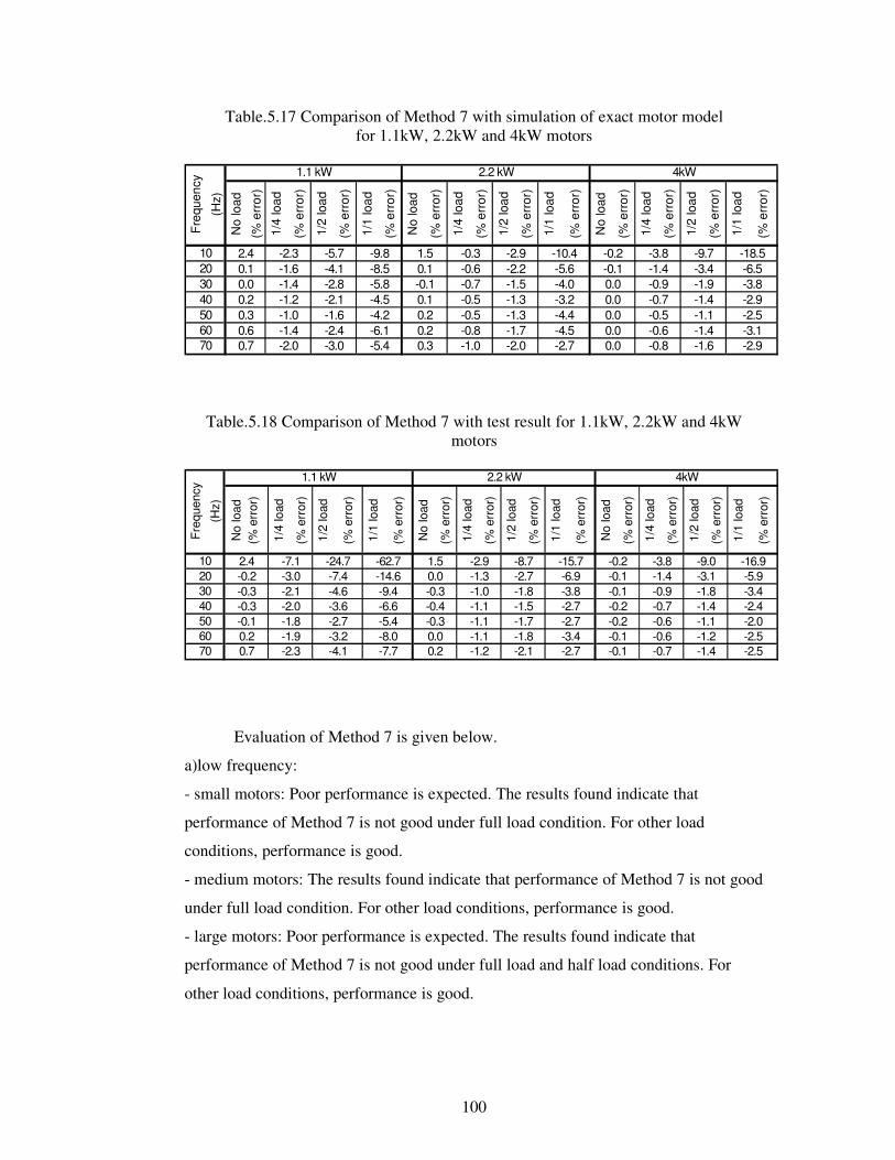
100

Table.5.17 Comparison of Method 7 with simulation of exact motor model for 1.1kW, 2.2kW and 4kW motors

No

load

(% e

rror

)

1/4

load

(% e

rror

)

1/2

load

(% e

rror

)

1/1

load

(% e

rror

)

No

load

(% e

rror

)

1/4

load

(% e

rror

)

1/2

load

(% e

rror

)

1/1

load

(% e

rror

)

No

load

(% e

rror

)

1/4

load

(% e

rror

)

1/2

load

(% e

rror

)

1/1

load

(% e

rror

)

-0.10.1

0.30.20.20.1 -0.5

-0.5-0.8-1.0

-2.9-0.3-0.6-0.7

-1.3-1.3-1.5-2.2

1.5

-2.7-4.5-4.4-3.2-4.0-5.6-10.4

-2.0-1.7-6.1

-4.2-4.5-5.8

0.20.00.12.4

-1.0-1.4-2.00.7

0.60.3

-2.3-1.6-1.4-1.2

-8.5-9.8

-3.0-2.4-1.6-2.1-2.8-4.1-5.7

-5.4

1.1 kW 4kW2.2 kW

Fre

quen

cy

(Hz)

70

50

30

10

60

40

20

-2.9-3.1-2.5-2.9-3.8-6.5-18.5

-1.6-1.4-1.1-1.4-1.9-3.4-9.7-3.8

-1.4-0.9-0.7-0.5-0.6-0.80.0

0.00.00.00.0-0.1-0.2

Table.5.18 Comparison of Method 7 with test result for 1.1kW, 2.2kW and 4kW motors

No

load

(%

err

or)

1/4

load

(% e

rror

)

1/2

load

(% e

rror

)

1/1

load

(% e

rror

)

No

load

(% e

rror

)

1/4

load

(% e

rror

)

1/2

load

(% e

rror

)

1/1

load

(% e

rror

)

No

load

(% e

rror

)

1/4

load

(% e

rror

)

1/2

load

(% e

rror

)

1/1

load

(% e

rror

)

-16.9

-8.0-5.4

-14.6-62.7

-2.1-3.0-7.1

-0.7-0.1

-0.1-0.2

-3.2

-1.4-0.9-0.7-0.6-0.6-0.1

-0.2-0.2-0.1

-2.3-1.9-1.8-2.0

1.1 kW 4kW2.2 kW

-1.2-1.1-1.4-1.8-3.1-9.0-3.8

Freq

uenc

y

(Hz)

70

50

30

10

60

40

20

0.7

2.4-0.2

-0.1-0.3-0.3

0.2-4.1

0.01.5

-5.9-3.4-2.4-2.0-2.5-2.5-1.4-7.7

-1.1-1.20.2

0.0

-9.4-6.6 -1.1

-1.1-0.3-0.4-0.3

-2.1-1.8-1.7-1.5 -2.7

-2.7-3.4-2.7

-2.7-3.6-4.6-7.4-24.7 -15.7

-6.9-3.8-1.8

-2.7-8.7-2.9

-1.3-1.0

Evaluation of Method 7 is given below.

a)low frequency:

- small motors: Poor performance is expected. The results found indicate that

performance of Method 7 is not good under full load condition. For other load

conditions, performance is good.

- medium motors: The results found indicate that performance of Method 7 is not good

under full load condition. For other load conditions, performance is good.

- large motors: Poor performance is expected. The results found indicate that

performance of Method 7 is not good under full load and half load conditions. For

other load conditions, performance is good.

101

b)medium frequency:

- small motors: Good performance is expected. The results found indicate that

performance of Method 7 is not good under full load condition. For other load

conditions, performance is good.

- medium motors: The results found indicate that performance of Method 7 is good for

all load conditions.

- large motors: Good performance is expected. The results found indicate that

performance of Method 7 is good for all load conditions.

c)high frequency:

- small motors: Good performance is expected. The results found indicate that

performance of Method 7 is not good under full load condition. For other load

conditions, performance is good.

- medium motors: The results found indicate that performance of Method 7 is good for

all load conditions.

- large motors: Good performance is expected. The results found indicate that

performance of Method 7 is good for all load conditions.

102

CHAPTER 6

CONCLUSION

The aim of this study is achieving speed estimation accuracy and torque

estimation accuracy with minimum number of calculations, minimum measurements

and minimum requirements for the motor parameters.

Some of the speed estimation methods require knowledge of motor parameters

for better speed estimation accuracy. Since no-load and locked rotor tests are

sometimes impractical to do and on-line parameter estimation methods place an

important burden of microprocessor, some methods are proposed to estimate motor

parameters off-line from manufacturer data. If the drive is capable of measuring

voltage and current off-line parameter measurement may also be possible.

Since manufacturer data may be erroneous, label data for motors is determined

from tests. When the parameter estimation results given in Chapter 2 are investigated,

it is seen that error of estimated parameters are very high. If average of these

estimation errors are taken for three test motors, averages of the errors are higher than

13% for 1.1kW motor, 25% for 2.2kW motor and 17% for 4kW motor.

Since these parameters are used to estimate torque-speed curve of the induction

motors, it is wise to compare the estimated torque-speed curves (at 50 Hz) which are

calculated from estimated parameters and parameters calculated from no-load and

locked rotor tests results. When the torque-speed curves calculated from estimated

parameters and parameters calculated from no-load and locked rotor tests results are

investigated, Method 4 given in Chapter 2 can be identified as the best parameter

estimation method giving overall good prediction for the whole torque-speed curve of

the three motors. This comparison is based on the starting torque, breakdown torque

and linear region of the torque-speed curve. Average of the error of estimated starting

103

torque is nearly 11% and average of the error of estimated breakdown torque is nearly

8% for Method 4.

Rated voltage, rated current, rated power factor, output power, frequency and

rated motor speed values are used in Method 4, which are all available on the motor

label.

Normally an induction motor is operated in the portion of torque-speed curve

between no-load speed and full-load speed. For this reason, the parameter predicted

from various methods discussed in Chapter 2 are also assesed regarding their accuracy

of prediction of the this region of the torque-speed characteristics. When the results are

investigated, again Method 4 is identified as the best estimation method giving good

prediction for the linear region of torque-speed curve.

At 50 Hz, when rated speed is taken as reference and comparison is based on

the torque prediction accuracy, torque prediction error of Method 4 is lower than 10%.

When torque is taken as reference and comparison is based on the speed, error of

Method 4 is nearly 1%. It must be noted however, that this error may be expected to be

larger at low speeds (frequencies).

Performances (stator current, rated torque and power factor) of the test motors

are calculated from estimated parameters and parameters from no-load and locked rotor

tests results are compared also with measured motor performance at rated torque

condition (50Hz). Comparisons are based on the torque, stator current and power factor

and average of the estimation errors are considered at rated speed. Method 3 and

Method 1 are better than other methods for 1.1kW motor. Method 2 is better than other

methods for 2.2kW motor. For 4kW motor, Method 2 and Method 3 are more suitable

than other methods. When all test motors are considered, Method 3 can be identified as

the best estimation method amongst these methods. In conclusion, it can be said that

the study in Chapter 2 led to methods of parameter prediction which give acceptably

good motor performance prediction at rated speed. In other words the methods

identified as better than others may be employed by an inexpensive drive, to predict

motor speed (from slow voltage and current measurements) and hence to control motor

speed or torque.

Since the most important aim of this study is achieving speed estimation

accuracy with minimum number of calculations and measurements, first speed

estimation methods found in literature are investigated. Two of these methods, suitable

104

for low cost motor drives, are briefly explained in Chapter3. Since these methods are

expected not to be suitable for heavy load conditions at low frequencies and in the field

weakening region, some methods are proposed to achieve speed estimation accuracy

with similar calculation burden for all load conditions and frequencies.

Since the best accuracy of speed prediction may be expected when the exact

induction motor model is used, as explained in Chapter3, initially accuracy of the exact

induction motor model is investigated. First a 2.2kW motor is driven from mains and

tests results are compared with simulation results. When rated speed is taken as

reference, measured torque is compared with estimated torque, prediction error is

found to be lower than 6%. However, when this comparison is repeated for inverter

driven 2.2kW motor, the torque prediction error is found to increase upto 14%.

When 2.2kW motor is driven with inverter at 50Hz, flux level is lower than

rated value since the dc link voltage does not permit higher voltage levels than applied.

Therefore, magnetizing reactance and core loss resistance is likely to be different from

the reference values obtained for rated flux. Furthermore, the pulsed waveform of the

inverter may affect the other parameters too. These may be the error sources. However,

this issue was not investigated further in this work.

As given above the best accuracy of speed prediction may be expected when the

exact induction motor model is used. Therefore, for evaluation of speed estimation

methods, speed estimation results are compared with simulation results of the exact

steady-state motor model.

Note that to have realistic simulation of the tests, in the simulation program

recorded voltage and current values are used for simulations.

In this study, medium frequency is defined as between 20 Hz and 50 Hz.

Frequencies over 50 Hz are named as high frequency. Low frequency is defined as

below 20Hz in this study. Since 1.1kW, 2.2kW and 4 kW motors are available in

laboratory and capacity of the inverter is not suitable for larger motors, these motors

are used in the experiments. In this study, 1.1 kW motor is named as small motor and

4kW motor is named as large motor. Since stator resistance of 2.2kW motor is smaller

than 4kW motor, 2.2kW motor can also be classified as a large motor.

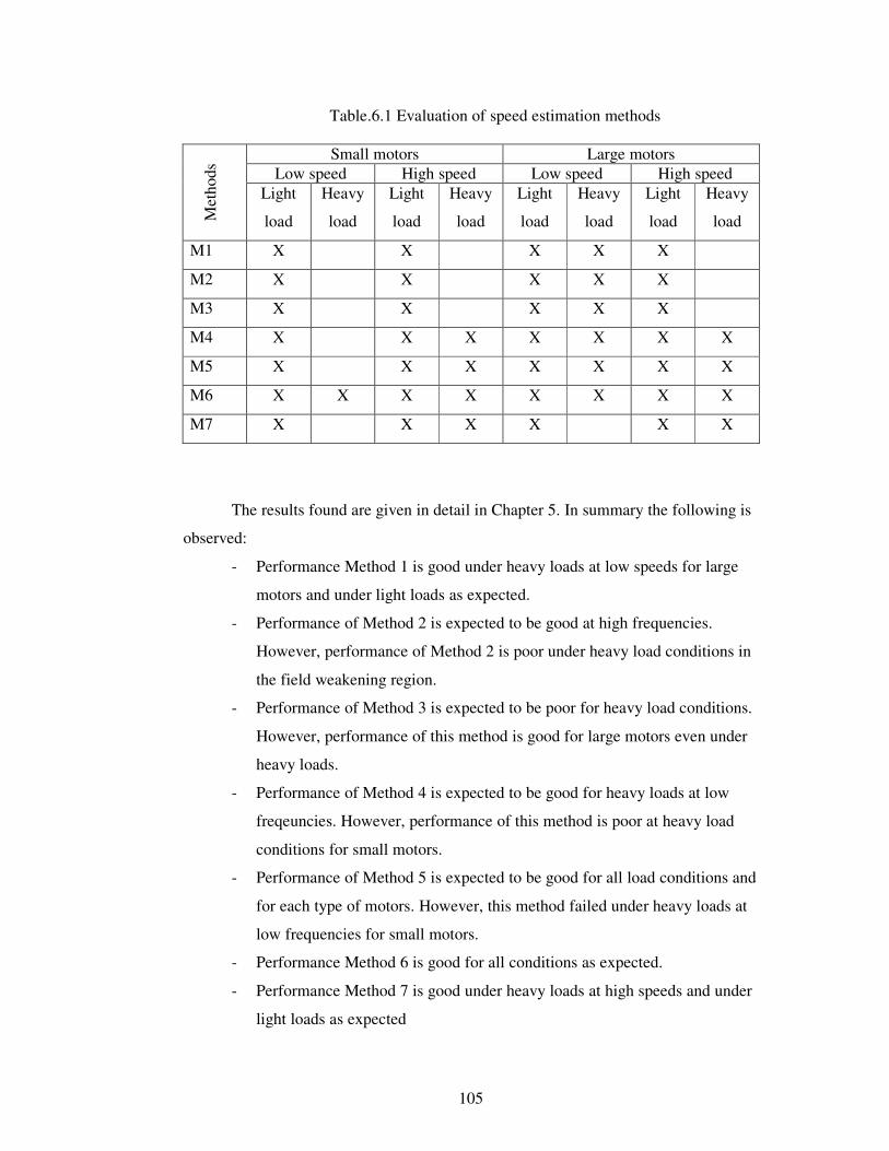
105

Table.6.1 Evaluation of speed estimation methods

Small motors Large motors Low speed High speed Low speed High speed

Met

hods

Light

load

Heavy

load

Light

load

Heavy

load

Light

load

Heavy

load

Light

load

Heavy

load

M1 X X X X X

M2 X X X X X

M3 X X X X X

M4 X X X X X X X

M5 X X X X X X X

M6 X X X X X X X X

M7 X X X X X X

The results found are given in detail in Chapter 5. In summary the following is

observed:

- Performance Method 1 is good under heavy loads at low speeds for large

motors and under light loads as expected.

- Performance of Method 2 is expected to be good at high frequencies.

However, performance of Method 2 is poor under heavy load conditions in

the field weakening region.

- Performance of Method 3 is expected to be poor for heavy load conditions.

However, performance of this method is good for large motors even under

heavy loads.

- Performance of Method 4 is expected to be good for heavy loads at low

freqeuncies. However, performance of this method is poor at heavy load

conditions for small motors.

- Performance of Method 5 is expected to be good for all load conditions and

for each type of motors. However, this method failed under heavy loads at

low frequencies for small motors.

- Performance Method 6 is good for all conditions as expected.

- Performance Method 7 is good under heavy loads at high speeds and under

light loads as expected

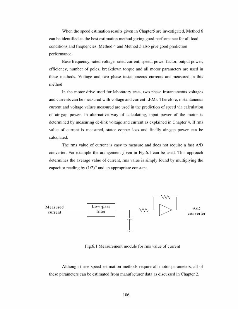
106

Low-passfilter

Measuredcurrent

A/Dconverter

When the speed estimation results given in Chapter5 are investigated, Method 6

can be identified as the best estimation method giving good performance for all load

conditions and frequencies. Method 4 and Method 5 also give good prediction

performance.

Base frequency, rated voltage, rated current, speed, power factor, output power,

efficiency, number of poles, breakdown torque and all motor parameters are used in

these methods. Voltage and two phase instantaneous currents are measured in this

method.

In the motor drive used for laboratory tests, two phase instantaneous voltages

and currents can be measured with voltage and current LEMs. Therefore, instantaneous

current and voltage values measured are used in the prediction of speed via calculation

of air-gap power. In alternative way of calculating, input power of the motor is

determined by measuring dc-link voltage and current as explained in Chapter 4. If rms

value of current is measured, stator copper loss and finally air-gap power can be

calculated.

The rms value of current is easy to measure and does not require a fast A/D

converter. For example the arangement given in Fig.6.1 can be used. This approach

determines the average value of current, rms value is simply found by multiplying the

capacitor reading by (1/2)½ and an appropriate constant.

Fig.6.1 Measurement module for rms value of current

Although these speed estimation methods require all motor parameters, all of

these parameters can be estimated from manufacturer data as discussed in Chapter 2.

107

Further work:

The remains much to be done:

a) Exact model of 1.1kW motor must be verified again.

b) Load tests can be repeated by using a torque transducer.

c) In order to reduce the necessity for usage of the motor parameters, breakdown

torque and slip under breakdown torque condition can be estimated. Effect of

these estimations to the speed prediction results can be examined.

d) The effect of inverter voltage waveform on motor parameters can be

investigated.

e) The effect of calculation of air-gap power by measuring dc-link voltage and

current and also measuring rms value of current can be investigated.

108

REFERENCES [1] Novotny, D.W., Lipo,T.A., “Vector Control and Dynamics of AC Drives", Oxford University Press, 1998 [2] Guzinski, J., Abu-Rub, H., Toliyat, H.A., “An Advanced Low-Cost Sensorless Induction Motor Drive”, APEC, 2002 [3] Finch, J.W., “Scalar and Vector: a Simplified Treatment of Induction Motor Control Performance”, Vector Control Revisited, IEE Colloquium on, 23 Feb.1998 [4] Abondanti, A., “Method of Flux Control in Induction Motors Driven by Variable Frequency, Variable Voltage Supplies”, IEEE/IAS Intl. Semi. Power Conv. Conf., 1977 [5] Krishnan, R. , “Electric Motor Drives: Modeling, Analysis, and Control”, Prentice-Hall, 2001 [6] Munoz-Garcia, A. , Lipo, T.A., Novotny, D.W., “A New Induction Motor Open-Loop Speed Control Capable of Low Frequency Operation”, IEEE Industry Applications Society Annual Meeting, 1997 [7] Lee, E.C., “Review of Variable Speed Drive Technology” , www.powertecmotors.com [8] Holtz, J., “Sensorless Control of Induction Motor Drives”, Proceedings of the IEEE, Aug.2002 [9] Garcia, G.O., Stephan, R.M., Watanabe, E.H., “Comparing the Indirect Field- Oriented Control with a Scalar Control”, IEEE Transactions on Industrial Electronics, April 1994 [10] Koga,K., Ueda,R., Sonoda,T., “Constitution of V/f Control for Reducing the Steady-State Speed Error to Zero in Induction Motor Drive System”, IEEE Transactions on Industry Applications, March/April 1992 [11] Bebic,M.Z., Jeftenic,B.I., Mitroviç,N.N., “A Simple Speed Sensorless Control for Variable Frequency Induction Motor Drives”, IEEE Transactions on Energy Conversion, September 1999 [12] Levi,E. , “Polyphase Motors”, Wiley & Sons, 1984

109

[13] Acar, A. , “Implementation of a vector controlled induction motor drive” , Msc. Thesis, METU, 2004 [14] Can, H.,“Implementation of vector control for induction motor”, Msc. Thesis, METU, 1999 [15] www.ti.com , “Space vector PWM with TMS320C24x using hardware and software determined switching patterns”, Application report SPRA524 [16] Murat, �.E. , “Self comissioning and on-line parameter identification of induction motors”, Msc. Thesis, METU, 2002 [17] Pedra, J. , Corcoles, F. , “Estimation of Induction Motor Double-Cage Model Parameters From Manufacturer Data”, IEEE Transactions on Energy Conversion, June 2004 [18] Vickers, H. , “The induction motor, the theory, design and application of alternating-current machines including fractional HP” , Pitman, 1953 [19] Jian Yu, Finch, J.V., “An alternative way to the scalar control of induction machines” ICEMS, 2001 [20] Krein P.T. , Disilvetsro F. , Kanellakopoulos I. , Locker J. , “Comparative analysis of scalar and vector control methods for induction motors” , PESC 1993 [21] Boys J.T. , Walton S.J. , “Scalar control : an alternative AC drive philosophy” IEEE Proceedings B [22] Briz F. , Diez A. , Degner M.W. , Lorenz R.D. , “Current and flux regulation in field weakening operation” , IAS’98 [23] Hurst K.D. , Habetler T.G. , Griva G. , Profumo F. , Jansen P.L. , “A self tuning closed loop flux observer for sensorless torque control standart induction machines” , IEEE transactions on power electronics september 1997 [24] Krzeminski Z. , “A new speed observer for control system of induction motor” , PEDS’99 [25] Yuenan Zeng , Yun Zhang , Duosheng Feng , “A new scheme of induction motor control for general purpose applications” , IPEMC 2000 [26] Lindenmeyer D. , Dommel H.W. , Moshref A., Kundur P., “An induction motor parameter estimation method” , International Journal of Electrical Power & Energy systems , May 2001 [27] Haque M.H. “ Estimation of 3-phase induction-motor parameters” , Electric power systems research, Apr 1993

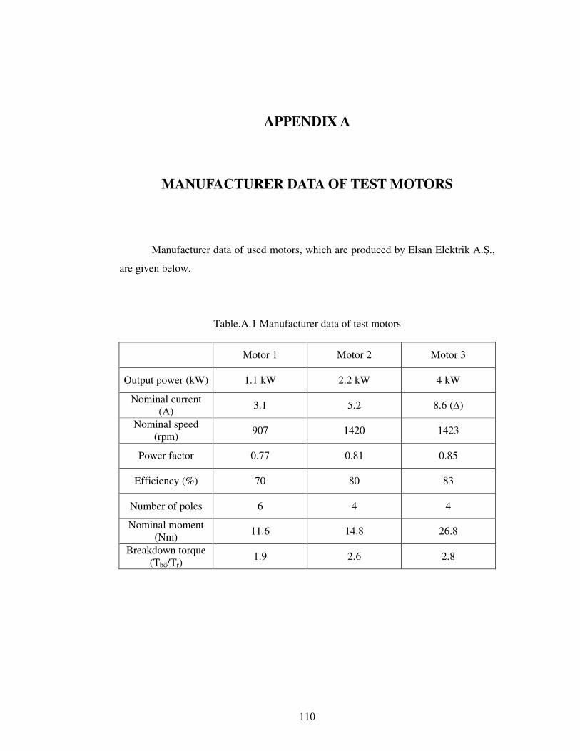
110

APPENDIX A

MANUFACTURER DATA OF TEST MOTORS

Manufacturer data of used motors, which are produced by Elsan Elektrik A.�.,

are given below.

Table.A.1 Manufacturer data of test motors

Motor 1 Motor 2 Motor 3

Output power (kW) 1.1 kW 2.2 kW 4 kW

Nominal current (A) 3.1 5.2 8.6 ( )

Nominal speed (rpm) 907 1420 1423

Power factor 0.77 0.81 0.85

Efficiency (%) 70 80 83

Number of poles 6 4 4

Nominal moment (Nm) 11.6 14.8 26.8

Breakdown torque (Tbd/Tr)

1.9 2.6 2.8

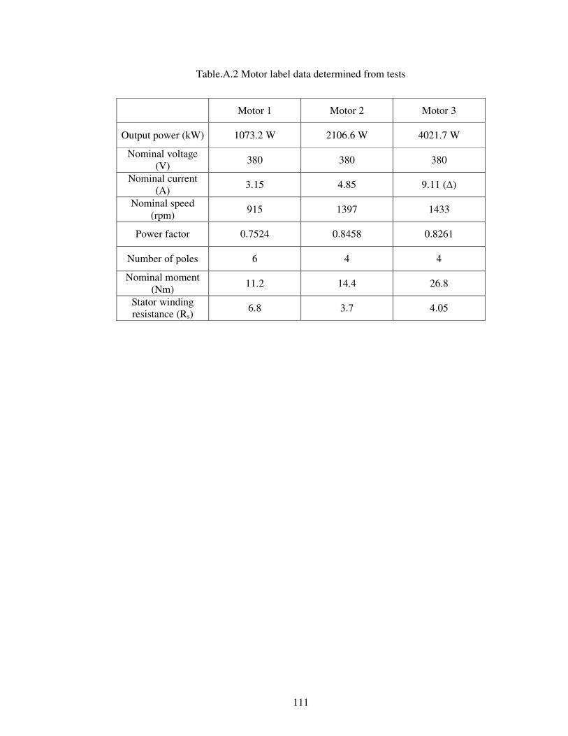
111

Table.A.2 Motor label data determined from tests

Motor 1 Motor 2 Motor 3

Output power (kW) 1073.2 W 2106.6 W 4021.7 W

Nominal voltage (V) 380 380 380

Nominal current (A) 3.15 4.85 9.11 ( )

Nominal speed (rpm) 915 1397 1433

Power factor 0.7524 0.8458 0.8261

Number of poles 6 4 4

Nominal moment (Nm) 11.2 14.4 26.8

Stator winding resistance (Rs)

6.8 3.7 4.05

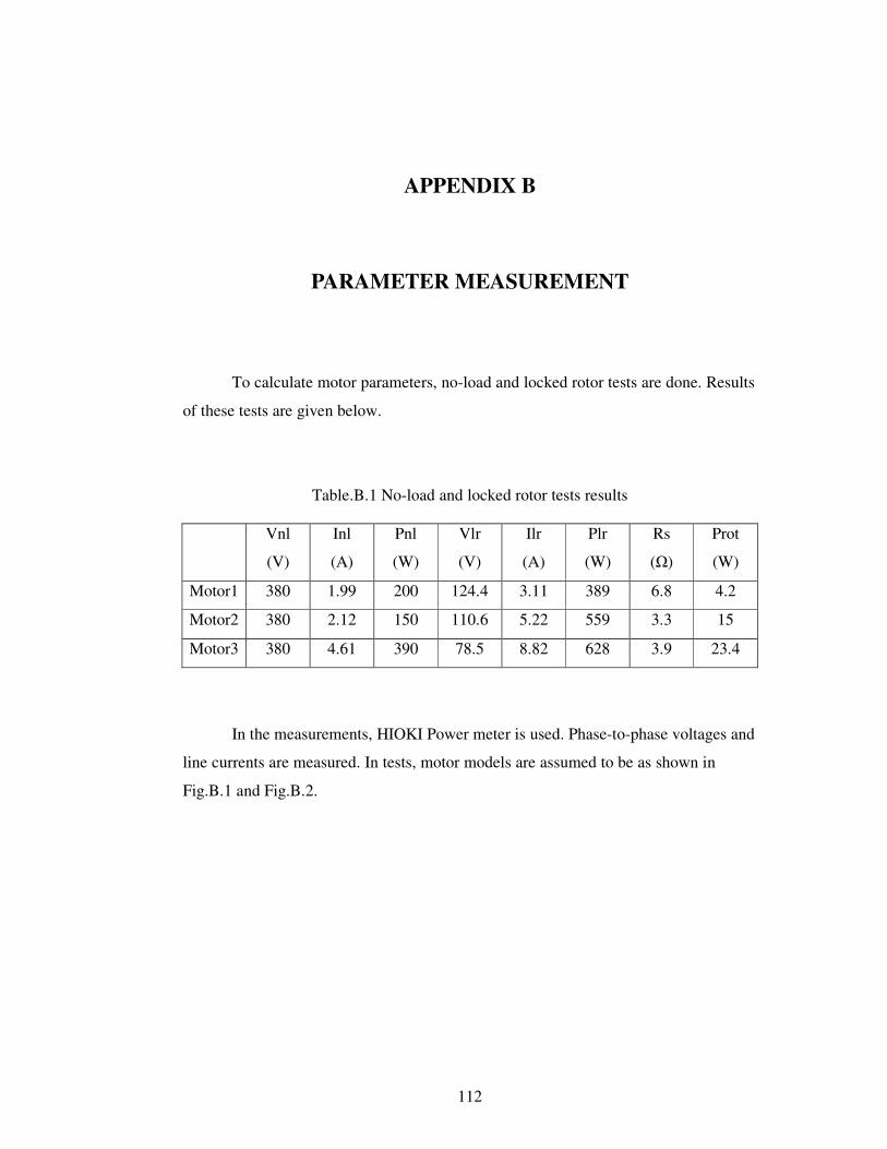
112

APPENDIX B

PARAMETER MEASUREMENT

To calculate motor parameters, no-load and locked rotor tests are done. Results

of these tests are given below.

Table.B.1 No-load and locked rotor tests results

Vnl

(V)

Inl

(A)

Pnl

(W)

Vlr

(V)

Ilr

(A)

Plr

(W)

Rs

(�)

Prot

(W)

Motor1 380 1.99 200 124.4 3.11 389 6.8 4.2

Motor2 380 2.12 150 110.6 5.22 559 3.3 15

Motor3 380 4.61 390 78.5 8.82 628 3.9 23.4

In the measurements, HIOKI Power meter is used. Phase-to-phase voltages and

line currents are measured. In tests, motor models are assumed to be as shown in

Fig.B.1 and Fig.B.2.

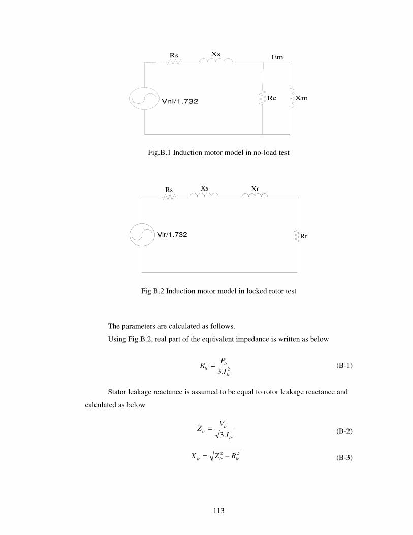
113

2.3 lr

lrlr I

PR =

lr

lrlr

IV

Z.3

=

22lrlrlr RZX −=

XsRs

Rc Xm

Em

Vnl/1.732

Fig.B.1 Induction motor model in no-load test

Vlr/1.732

XsRs Xr

Rr

Fig.B.2 Induction motor model in locked rotor test The parameters are calculated as follows.

Using Fig.B.2, real part of the equivalent impedance is written as below

(B-1)

Stator leakage reactance is assumed to be equal to rotor leakage reactance and

calculated as below

(B-2)

(B-3)

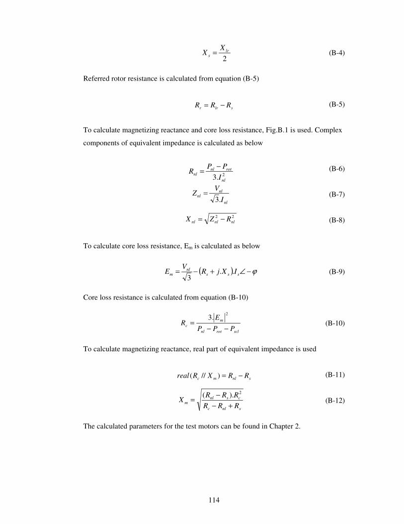
114

2lr

s

XX =

slrr RRR −=

2.3 nl

rotnlnl I

PPR

−=

nl

nlnl

IV

Z.3

=

22nlnlnl RZX −=

( ) ϕ−∠+−= sssnl

m IXjRV

E ..3

sclrotnl

mc PPP

ER

−−=

2.3

snlmc RRXRreal −=)//(

snlc

csnlm RRR

RRRX

+−−=

2).(

(B-4)

Referred rotor resistance is calculated from equation (B-5)

(B-5)

To calculate magnetizing reactance and core loss resistance, Fig.B.1 is used. Complex

components of equivalent impedance is calculated as below

(B-6)

(B-7)

(B-8)

To calculate core loss resistance, Em is calculated as below

(B-9)

Core loss resistance is calculated from equation (B-10)

(B-10)

To calculate magnetizing reactance, real part of equivalent impedance is used

(B-11)

(B-12)

The calculated parameters for the test motors can be found in Chapter 2.

115

APPENDIX C

PARAMETER ESTIMATION CODES

C-1 Method 1

Rs=6.6;

Rs=Rs*1.1;

V=220;

I=3.1;

f=50; input data

pf=0.74;

p=6;

n=907;

Pout=1100;

%%%%%%%%%%%%%%%%%%%%%%%%%%%%%

fi=acos(pf);

ns=120*f/p;

s=(ns-n)/ns;

Pfw=0.01*Pout;

Prcl=(Pout+Pfw)*s/(1-s); calculation of Rr

a=Prcl/s^2;

b=(2*Rs*Prcl/s)-(3*V^2);

c=Prcl*Rs^2;

delta=b^2-4*a*c;

Rr=(-b+sqrt(delta))/(2*a)

%%%%%%%%%%%%%%%%%%%%%%%%%%%%%

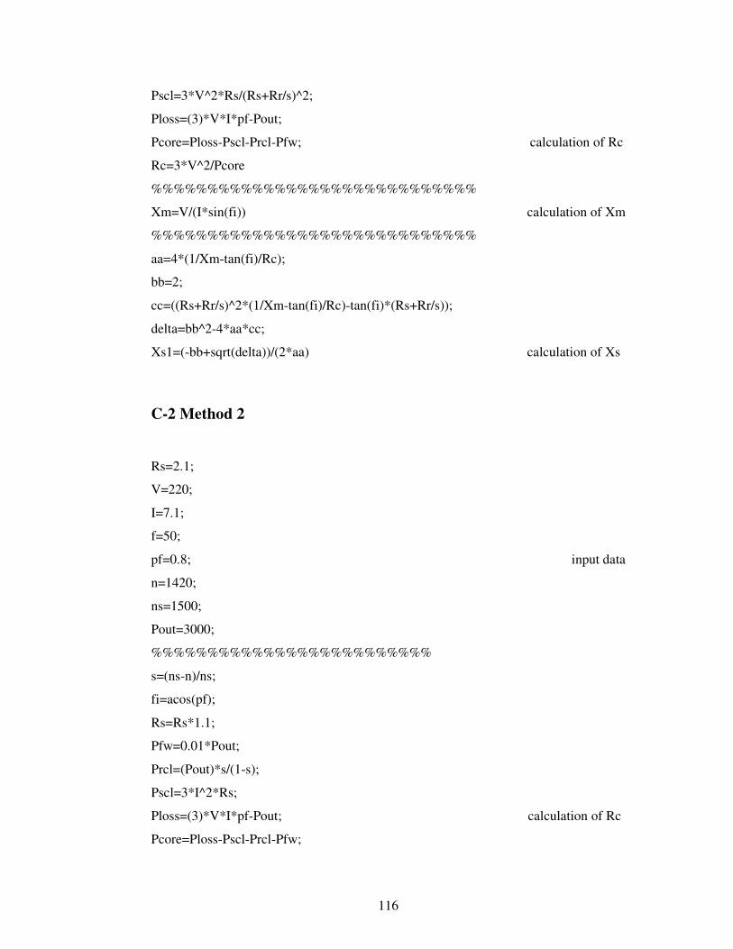
116

Pscl=3*V^2*Rs/(Rs+Rr/s)^2;

Ploss=(3)*V*I*pf-Pout;

Pcore=Ploss-Pscl-Prcl-Pfw; calculation of Rc

Rc=3*V^2/Pcore

%%%%%%%%%%%%%%%%%%%%%%%%%%%%%

Xm=V/(I*sin(fi)) calculation of Xm

%%%%%%%%%%%%%%%%%%%%%%%%%%%%%

aa=4*(1/Xm-tan(fi)/Rc);

bb=2;

cc=((Rs+Rr/s)^2*(1/Xm-tan(fi)/Rc)-tan(fi)*(Rs+Rr/s));

delta=bb^2-4*aa*cc;

Xs1=(-bb+sqrt(delta))/(2*aa) calculation of Xs

C-2 Method 2

Rs=2.1;

V=220;

I=7.1;

f=50;

pf=0.8; input data

n=1420;

ns=1500;

Pout=3000;

%%%%%%%%%%%%%%%%%%%%%%%%%

s=(ns-n)/ns;

fi=acos(pf);

Rs=Rs*1.1;

Pfw=0.01*Pout;

Prcl=(Pout)*s/(1-s);

Pscl=3*I^2*Rs;

Ploss=(3)*V*I*pf-Pout; calculation of Rc

Pcore=Ploss-Pscl-Prcl-Pfw;

117

Rc=3*V^2/Pcore

%%%%%%%%%%%%%%%%%%%%%%%%

Xm=V/(I*sin(fi)) calculation of Xm

%%%%%%%%%%%%%%%%%%%%%%%%

a=(tan(fi))^2/s^2+(3*V^2/Prcl)^2*(tan(fi)/Rc-

1/Xm)^2+6*V^2*tan(fi)/(s*Prcl)*(tan(fi)/Rc-1/Xm)+1/s^2;

b=2*Rs*(tan(fi))^2/s+6*V^2*Rs*tan(fi)/Prcl*(tan(fi)/Rc-1/Xm)+2*Rs/s-3*V^2/Prcl;

c=(Rs*tan(fi))^2+Rs^2; calculation of Rr

delta=b^2-4*a*c;

Rr=(-b+sqrt(delta))/(2*a)

%%%%%%%%%%%%%%%%%%%%%%%%

Xs=sqrt((3*V^2*Rr/Prcl-(Rs+Rr/s)^2)/4) calculation of Xs

C-3 Method 3 & Method 4

V=220;

R1=4.5;

R1=1.1*R1;

I=2.7;

Pout=1000;

Pfric=0.01*Pout;

ws=3000;

wm=2830;

pf=0.76;

%%%%%%%%%%%%%%%

fi=acos(pf);

tn1=tan(fi)

s=(ws-wm)/ws;

Prcl=(Pout+Pfric)*(s/(1-s));

Pin=3*V*I*pf;

Pcore=Pin-Pout-(3*I^2*R1)-Prcl-Pfric;

Pgap=Pout+Pfric+Prcl;

118

n=20;

X1=0;

tum_sonuc=[];

while (n>0)

E=(V-(R1+X1*i)*(I*cos(fi)-I*sin(fi)*i));

E=abs(E);

a=Prcl/(s^2);

b=(-3)*E^2;

c=Prcl*X1^2;

delta=b^2-4*a*c;

if delta<0

disp ('kökler imajiner')

else

R2=((-b)+sqrt(delta))/(2*a);

end

Rc=(3*E^2/Pcore);

Xm=E/(1*I*sin(fi));

aa=R2^2/s^2;

bb=(2*R1*R2*Xm^2/s)-(3*V^2*R2*Xm^2/(s*Pgap));

cc=R1^2*Xm^4;

delta2=bb^2-4*aa*cc;

if delta2<0

disp ('kökler imajiner')

else

dd=(-bb+sqrt(delta2))/(2*aa);

end

X1=(sqrt(dd)-Xm);

a=(Xm*R2/s+Rc*X1+Rc*Xm);

b=(X1*Xm-Rc*R2/s);

tn=(X1*(a^2+b^2)+a*(X1*Xm*Rc)-

b*(Rc*Xm*R2/s))/(R1*(a^2+b^2)+a*(Rc*Xm*R2/s)+b*(X1*Xm*Rc));

n=n-1;

sonuc=[R1 R2 X1 Xm Rc tn];

119

tum_sonuc=[tum_sonuc; sonuc];

end

C-4 Method 5

v=220;

Is=7.1;

rs=2.1;

Pout=3000;

pole=4;

f=50;

nm=1420;

pf=0.8;

%%%%%%%%

sonuc=[];

tumsonuc=[];

n=120*f/pole;

w=4*pi*f/pole;

s=(n-nm)/n;

fi=acos(pf);

Pin=3*v*Is*pf;

eff=Pout/Pin;

Im=0.95*Is*sin(fi);

xm=(v-rs*Is)/Im

Ir=sqrt(Is^2-(Im)^2);

xs=(3*v*Is*sin(fi)-3*xm*(Im)^2)/(3*Is^2+3*Ir^2);

Piron=Pin*(1-eff/(1-s))-3*rs*Is^2;

rc=3*v^2/Piron;

i=1;

while i>0

Ir=sqrt(Is^2-(Im)^2)-(v-rs*Is)/rc;

xs=(3*v*Is*sin(fi)-3*xm*(Im)^2)/(3*Is^2+3*Ir^2)

120

Pmec=0.005*Pout;

Pstr=0.005*Pout;

Tem=(Pout+Pmec)/((1-s)*w);

rr=Tem*s*w/(3*Ir^2)

Piron=Pin-3*rs*Is^2-Pstr-3*(rr/s)*Ir^2;

i=i-1;

Em=v-(rs+xs*i)*Is*(cos(fi)-sin(fi)*i);

Em=abs(Em);

rc=3*Em^2/Piron

sonuc=[rr xs xm rc];

tumsonuc=[tumsonuc; sonuc];

end

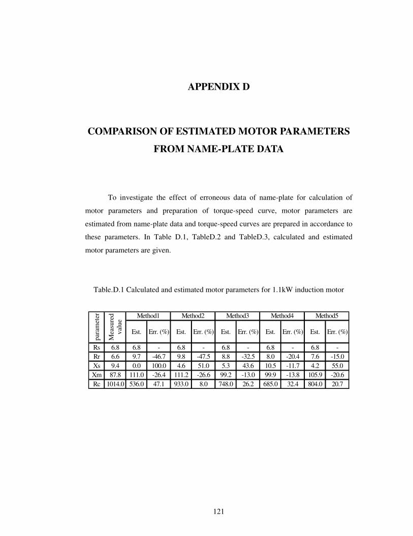
121

APPENDIX D

COMPARISON OF ESTIMATED MOTOR PARAMETERS

FROM NAME-PLATE DATA

To investigate the effect of erroneous data of name-plate for calculation of

motor parameters and preparation of torque-speed curve, motor parameters are

estimated from name-plate data and torque-speed curves are prepared in accordance to

these parameters. In Table D.1, TableD.2 and TableD.3, calculated and estimated

motor parameters are given.

Table.D.1 Calculated and estimated motor parameters for 1.1kW induction motor

Est. Err. (%) Est. Err. (%) Est. Err. (%) Est. Err. (%) Est. Err. (%)

Rs 6.8 6.8 - 6.8 - 6.8 - 6.8 - 6.8 -Rr 6.6 9.7 -46.7 9.8 -47.5 8.8 -32.5 8.0 -20.4 7.6 -15.0Xs 9.4 0.0 100.0 4.6 51.0 5.3 43.6 10.5 -11.7 4.2 55.0Xm 87.8 111.0 -26.4 111.2 -26.6 99.2 -13.0 99.9 -13.8 105.9 -20.6Rc 1014.0 536.0 47.1 933.0 8.0 748.0 26.2 685.0 32.4 804.0 20.7

Method3 Method4 Method5

para

met

er

Mea

sure

d va

lue

Method1 Method2

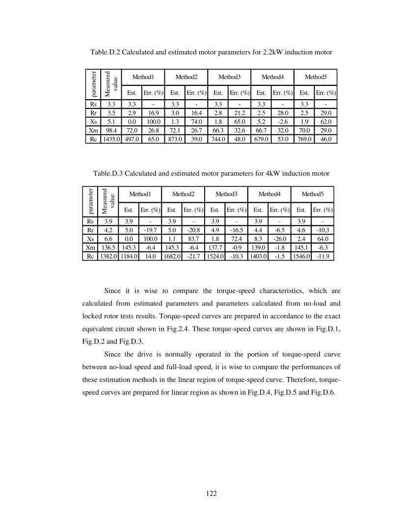
122

Table.D.2 Calculated and estimated motor parameters for 2.2kW induction motor

Est. Err. (%) Est. Err. (%) Est. Err. (%) Est. Err. (%) Est. Err. (%)

Rs 3.3 3.3 - 3.3 - 3.3 - 3.3 - 3.3 -Rr 3.5 2.9 16.9 3.0 16.4 2.8 21.2 2.5 28.0 2.5 29.0Xs 5.1 0.0 100.0 1.3 74.0 1.8 65.0 5.2 -2.6 1.9 62.0Xm 98.4 72.0 26.8 72.1 26.7 66.3 32.6 66.7 32.0 70.0 29.0Rc 1435.0 497.0 65.0 873.0 39.0 744.0 48.0 679.0 53.0 769.0 46.0

Method3 Method4 Method5

para

met

er

Mea

sure

d va

lue Method1 Method2

Table.D.3 Calculated and estimated motor parameters for 4kW induction motor

Est. Err. (%) Est. Err. (%) Est. Err. (%) Est. Err. (%) Est. Err. (%)

Rs 3.9 3.9 - 3.9 - 3.9 - 3.9 - 3.9 -Rr 4.2 5.0 -19.7 5.0 -20.8 4.9 -16.5 4.4 -6.5 4.6 -10.3Xs 6.6 0.0 100.0 1.1 83.7 1.8 72.4 8.3 -26.0 2.4 64.0Xm 136.5 145.3 -6.4 145.3 -6.4 137.7 -0.9 139.0 -1.8 145.1 -6.3Rc 1382.0 1184.0 14.0 1682.0 -21.7 1524.0 -10.3 1403.0 -1.5 1546.0 -11.9

Method3 Method4 Method5

para

met

er

Mea

sure

d va

lue Method1 Method2

Since it is wise to compare the torque-speed characteristics, which are

calculated from estimated parameters and parameters calculated from no-load and

locked rotor tests results. Torque-speed curves are prepared in accordance to the exact

equivalent circuit shown in Fig.2.4. These torque-speed curves are shown in Fig.D.1,

Fig.D.2 and Fig.D.3.

Since the drive is normally operated in the portion of torque-speed curve

between no-load speed and full-load speed, it is wise to compare the performances of

these estimation methods in the linear region of torque-speed curve. Therefore, torque-

speed curves are prepared for linear region as shown in Fig.D.4, Fig.D.5 and Fig.D.6.

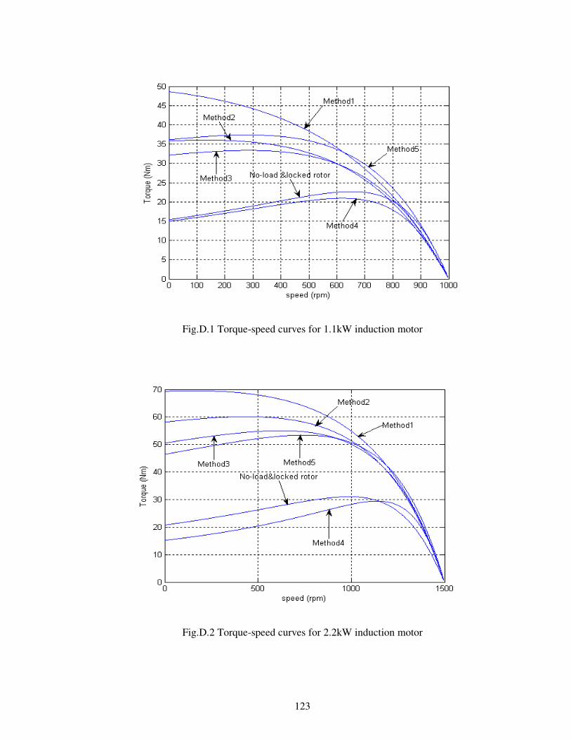
123

Fig.D.1 Torque-speed curves for 1.1kW induction motor

Fig.D.2 Torque-speed curves for 2.2kW induction motor

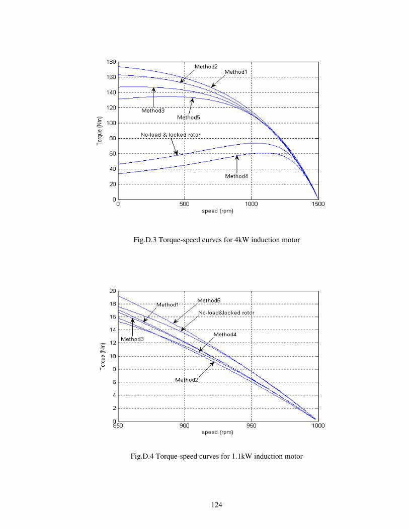
124

Fig.D.3 Torque-speed curves for 4kW induction motor

Fig.D.4 Torque-speed curves for 1.1kW induction motor

125

Fig.D.5 Torque-speed curves for 2.2kW induction motor

Fig.D.6 Torque-speed curves for 4kW induction motor

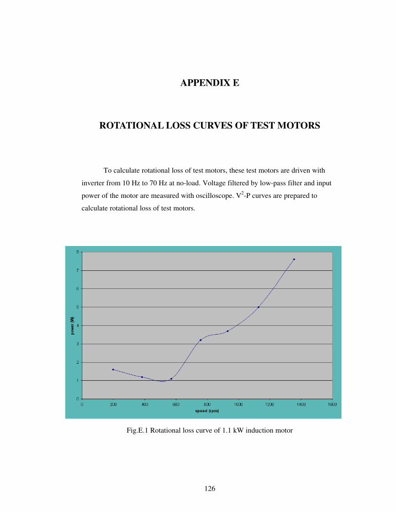
126

APPENDIX E

ROTATIONAL LOSS CURVES OF TEST MOTORS

To calculate rotational loss of test motors, these test motors are driven with

inverter from 10 Hz to 70 Hz at no-load. Voltage filtered by low-pass filter and input

power of the motor are measured with oscilloscope. V2-P curves are prepared to

calculate rotational loss of test motors.

Fig.E.1 Rotational loss curve of 1.1 kW induction motor

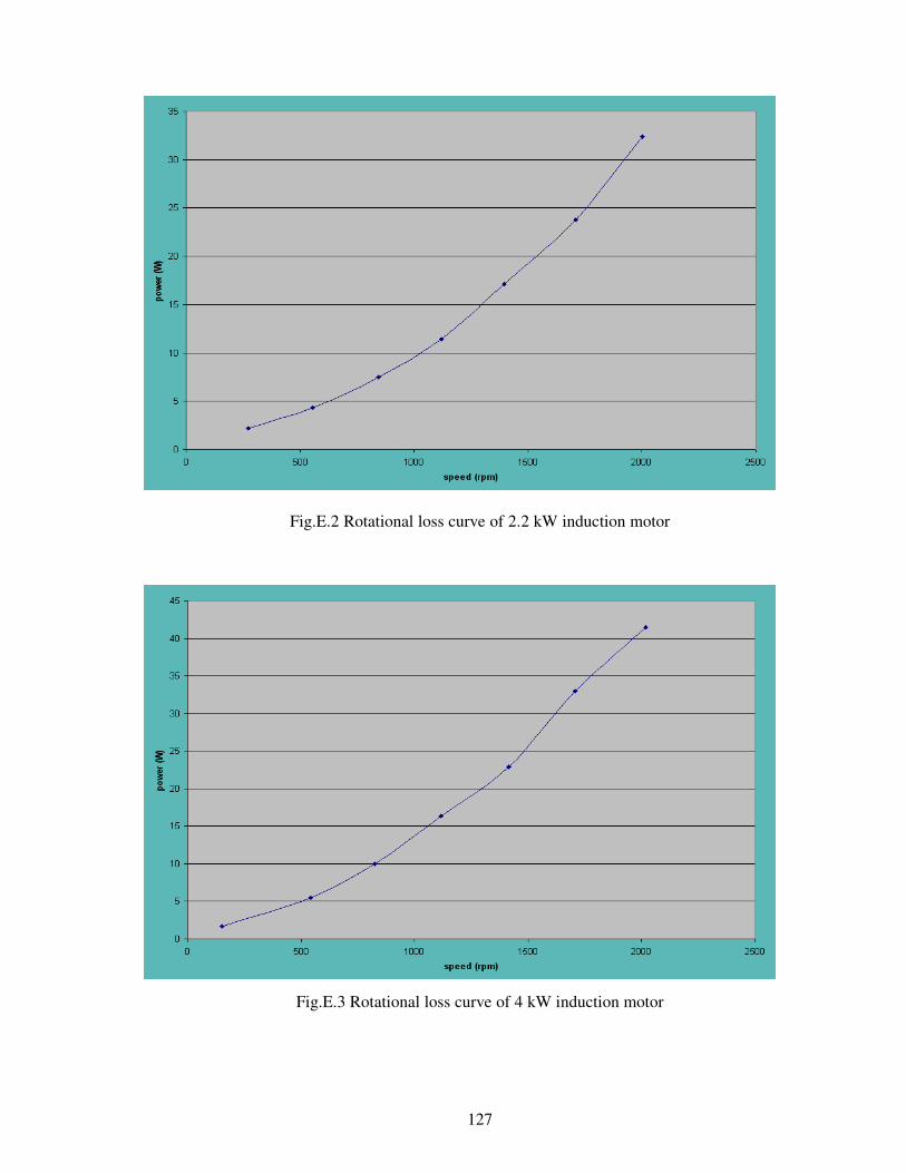
127

Fig.E.2 Rotational loss curve of 2.2 kW induction motor

Fig.E.3 Rotational loss curve of 4 kW induction motor

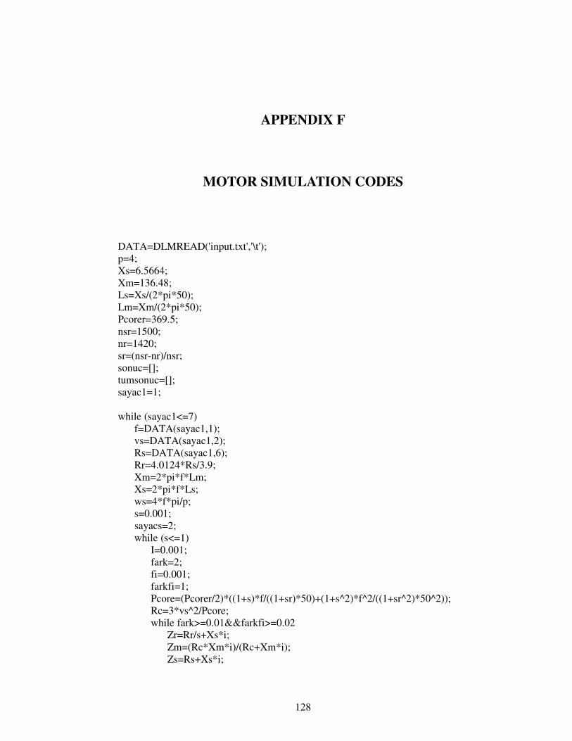
128

APPENDIX F

MOTOR SIMULATION CODES

DATA=DLMREAD('input.txt','\t'); p=4; Xs=6.5664; Xm=136.48; Ls=Xs/(2*pi*50); Lm=Xm/(2*pi*50); Pcorer=369.5; nsr=1500; nr=1420; sr=(nsr-nr)/nsr; sonuc=[]; tumsonuc=[]; sayac1=1; while (sayac1<=7) f=DATA(sayac1,1); vs=DATA(sayac1,2); Rs=DATA(sayac1,6); Rr=4.0124*Rs/3.9; Xm=2*pi*f*Lm; Xs=2*pi*f*Ls; ws=4*f*pi/p; s=0.001; sayacs=2; while (s<=1) I=0.001; fark=2; fi=0.001; farkfi=1; Pcore=(Pcorer/2)*((1+s)*f/((1+sr)*50)+(1+s^2)*f^2/((1+sr^2)*50^2)); Rc=3*vs^2/Pcore; while fark>=0.01&&farkfi>=0.02 Zr=Rr/s+Xs*i; Zm=(Rc*Xm*i)/(Rc+Xm*i); Zs=Rs+Xs*i;

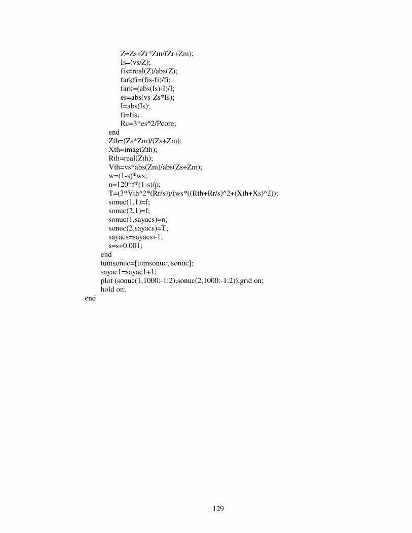
129

Z=Zs+Zr*Zm/(Zr+Zm); Is=(vs/Z); fis=real(Z)/abs(Z); farkfi=(fis-fi)/fi; fark=(abs(Is)-I)/I; es=abs(vs-Zs*Is); I=abs(Is); fi=fis; Rc=3*es^2/Pcore; end Zth=(Zs*Zm)/(Zs+Zm); Xth=imag(Zth); Rth=real(Zth); Vth=vs*abs(Zm)/abs(Zs+Zm); w=(1-s)*ws; n=120*f*(1-s)/p; T=(3*Vth^2*(Rr/s))/(ws*((Rth+Rr/s)^2+(Xth+Xs)^2)); sonuc(1,1)=f; sonuc(2,1)=f; sonuc(1,sayacs)=n; sonuc(2,sayacs)=T; sayacs=sayacs+1; s=s+0.001; end tumsonuc=[tumsonuc; sonuc]; sayac1=sayac1+1; plot (sonuc(1,1000:-1:2),sonuc(2,1000:-1:2)),grid on; hold on; end

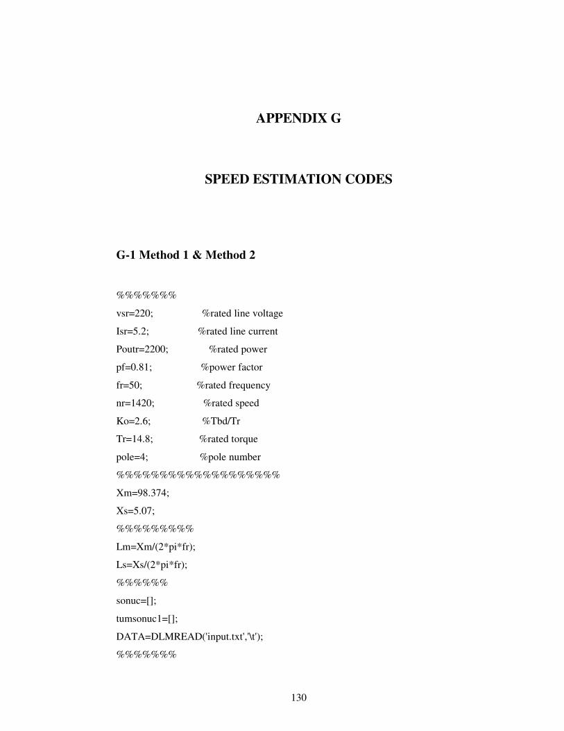
130

APPENDIX G

SPEED ESTIMATION CODES

G-1 Method 1 & Method 2

%%%%%%%

vsr=220; %rated line voltage

Isr=5.2; %rated line current

Poutr=2200; %rated power

pf=0.81; %power factor

fr=50; %rated frequency

nr=1420; %rated speed

Ko=2.6; %Tbd/Tr

Tr=14.8; %rated torque

pole=4; %pole number

%%%%%%%%%%%%%%%%%%%

Xm=98.374;

Xs=5.07;

%%%%%%%%%

Lm=Xm/(2*pi*fr);

Ls=Xs/(2*pi*fr);

%%%%%%

sonuc=[];

tumsonuc1=[];

DATA=DLMREAD('input.txt','\t');

%%%%%%%

131

sayac1=1;

while sayac1 <=7

hiz=DATA(sayac1,3);

fm=DATA(sayac1,1);

f=fm;

vs=DATA(sayac1,2);

Rs=DATA(sayac1,6);

Rr=3.43*Rs/3.2;

%%%%%%%%

ns=120*f/pole;

w=ns*pi/30;

s=(ns-hiz)/ns;

Pinr=3*vsr*Isr*pf;

eff=Poutr/Pinr;

nsr=120*fr/pole;

sr=(nsr-nr)/nsr;

Pcorer=160.8;

%%%%%%%%%

Xm=Lm*2*pi*f;

Xs=Ls*2*pi*f;

Rth=Rs*(Xm/(Xm+Xs))^2;

Vth=vs*Xm/(Xs+Xm);

Tm=3*Vth^2/(2*w*(Rth+sqrt(Rth^2+4*Xs^2)));

sm=Rr/sqrt(Rth^2+4*Xs^2);

%%%%%%%%%%%%%%%%%%%%%%

Is=DATA(sayac1,4);

Is_real=DATA(sayac1,5);

%%%%%%%%%%%%%%%%%%%%%%%%%%

es=vs-Rs*Is;

es=abs(es);

%%%%%%%%%%

Pcore=(Pcorer/2)*((1+s)*f/((1+sr)*fr)+(1+s^2)*f^2/((1+sr^2)*fr^2));

Pgap=3*vs*Is_real-3*Rs*Is^2-Pcore;

132

K=Ko+sqrt(Ko^2-1);

slin=pole*sr*fr/(Tr*pi);

A=pole/(4*pi*K*Ko*Tr*sr*fr);

B=(pole/(4*pi*Ko*Tr))^2;

C=A*Pgap;

if C==2

f_slip=B/(A*fm);

else

f_slip=(sqrt(fm^2+(K*slin*Pgap/(2*Ko))-B*Pgap^2)-fm)/(2-A*Pgap);

end

n_slip=120*f_slip/pole;

n_slip=abs(n_slip);

n1=ns-n_slip;

n1=abs(n1);

err1=(hiz-n1)*100/hiz;

%%%%%%%%%%%%

%%%%method 2

Ko2=Tm/Tr;

K=Ko2+sqrt(Ko2^2-1);

A=pole/(4*pi*K*Ko2*Tr*sr*fr);

B=(pole/(4*pi*Ko2*Tr))^2;

C=A*Pgap;

if C==2

f_slip=B/(A*fm);

else

f_slip=(sqrt(fm^2+(K*slin*Pgap/(2*Ko2))-B*Pgap^2)-fm)/(2-A*Pgap);

end

n_slip=120*f_slip/pole;

n_slip=abs(n_slip);

n2=ns-n_slip;

n2=abs(n2);

err2=(hiz-n2)*100/hiz;

sonuc=[hiz n1 err1 n2 err2];

133

tumsonuc1=[tumsonuc1; sonuc];

sayac1=sayac1+1;

end

G-2 Method 3 & Method 4 & Method 5

Vsr=220;

pf=0.81;

Isr=5.2;

Poutr=2200;

fr=50;

p=4;

nr=1420;

Ko=2.6;

%%%%%%%%

Xm=98.374;

Xs=5.07;

%%%%%%%%

Lm=Xm/(2*pi*fr);

Ls=Xs/(2*pi*fr);

%%%%%%%%

sonuc=[];

tumsonuc2=[];

DATA=DLMREAD('input.txt','\t');

%%%%%%%%%%%%%%%%

sayac1=1;

while sayac1 <=7

%%%%%%%%%%

hiz=DATA(sayac1,3);

nm=hiz;

f=DATA(sayac1,1);

fm=f;

134

vs=DATA(sayac1,2);

Rs=DATA(sayac1,6);

Rr=3.43*Rs/3.2;

%%%%%%%%%%%METHOD 4 & METHOD 5

Xm=Lm*2*pi*f;

Xs=Ls*2*pi*f;

n=120*f/p;

nsr=120*fr/p;

w=n*pi/30;

wr=nr*pi/30;

Tr=Poutr/wr;

Rth=Rs*(Xm/(Xm+Xs))^2;

Vth=vs*Xm/(Xs+Xm);

Tm=3*Vth^2/(2*w*(Rth+sqrt(Rth^2+4*Xs^2)));

sm=Rr/sqrt(Rth^2+4*Xs^2);

%%%%%%

Is=DATA(sayac1,4);

Is_real=DATA(sayac1,5);

%%%%%%%%%

nsr=120*fr/p;

sr=(nsr-nr)/nsr;

s=(n-nm)/n;

%%%%%%%%

Pinr=3*Vsr*Isr*pf;

eff=Poutr/Pinr;

Pcorer=160.8;

Pcore=(Pcorer/2)*((1+s)*f/((1+sr)*fr)+(1+s^2)*f^2/((1+sr^2)*fr^2));

%%%%%%%%

Pin=3*vs*Is_real;

Pscl=3*Rs*(abs(Is))^2;

Pgap=Pin-Pscl-Pcore;

Pgap=abs(Pgap);

T=Pgap/w;

135

%%%%%%%%

a=Rs/Rr;

b=2*a*sm;

c=2*Tm*(1+a*sm);

d=(c-b*T)/T;

delta=(d*sm)^2-4*sm^2;

s=(d*sm-sqrt(delta))/2;

s=abs(s);

speed4a=120*f*(1-s)/p;

speed4a=abs(speed4a);

err4a=(hiz-speed4a)*100/hiz;

%%%%%%%%

a=Rth/Rr;

b=2*a*sm;

c=2*Tm*(1+a*sm);

d=(c-b*T)/T;

delta=(d*sm)^2-4*sm^2;

s=(d*sm-sqrt(delta))/2;

s=abs(s);

speed5a=120*f*(1-s)/p;

speed5a=abs(speed5a);

err5a=(hiz-speed5a)*100/hiz;

%%%%%%%%method 3

sl=T*(nsr-nr)/Tr;

sl=abs(sl);

n3=n-sl;

n3=abs(n3);

err3=(hiz-n3)*100/hiz;

sonuc=[n3 err3 speed4a err4a speed5a err5a];

tumsonuc2=[tumsonuc2; sonuc];

sayac1=sayac1+1;

end

136

G-3 Method 6 & Method 7

Vsr=220;

pf=0.81;

Isr=5.2;

Poutr=2200;

fr=50;

p=4;

nr=1420;

%%%%%%%%

Ko=2.6;

Xm=98.374;

Xs=5.07;

Ls=Xs/(2*pi*fr);

Lm=Xm/(2*pi*fr);

%%%%%%%%

sonuc=[];

tumsonuc3=[];

DATA=DLMREAD('input.txt','\t');

%%%%%%%%%%%%%%%%

sayac1=1;

while sayac1 <=7

%%%%%%%%%%%%%%%

hiz=DATA(sayac1,3);

nm=hiz;

f=DATA(sayac1,1);

fm=f;

vs=DATA(sayac1,2);

Rs=DATA(sayac1,6);

Rr=3.43*Rs/3.2;

%%%%%%%%

n=120*f/p;

w=n*pi/30;

137

wr=nr*pi/30;

nsr=120*fr/p;

sr=(nsr-nr)/nsr;

Tr=Poutr/wr;

%%%%%%%%%

Xm=Lm*2*pi*f;

Xs=Ls*2*pi*f;

Rth=Rs*(Xm/(Xm+Xs))^2;

Vth=vs*Xm/(Xs+Xm);

Tm=3*Vth^2/(2*w*(Rth+sqrt(Rth^2+4*Xs^2)));

sm=Rr/sqrt(Rth^2+4*Xs^2);

%%%%%%%%%%%%%

s=(n-nm)/n;

%%%%%%%%%%%

Is=DATA(sayac1,4);

Is_real=DATA(sayac1,5);

%%%%%%%%%%%%%%%%%%%%%%%%%%%

es=vs-Rs*Is;

es=abs(es);

%%%%%%%%

Pinr=3*Vsr*Isr*pf;

eff=Poutr/Pinr;

s=(n-nm)/n;

Pcorer=160.8;

Pcore=(Pcorer/2)*((1+s)*f/((1+sr)*fr)+(1+s^2)*f^2/((1+sr^2)*fr^2));

%%%%%%%%

Pin=3*vs*Is_real;

Pscl=3*Rs*(abs(Is))^2;

Pgap=Pin-Pscl-Pcore;

Pgap=abs(Pgap);

T=Pgap/w;

%%%%%%%%

Xm=2*pi*f*Lm;

138

Xs=2*pi*f*Ls;

Z=(Xm*i)*(Rr/sm+Xs*i)/(Rr/sm+Xs*i+Xm*i);

Ism=vs/(Rs+2*pi*f*Ls*i+Z);

esm=vs-Rs*Ism;

esm=abs(esm);

a=es/esm;

b=((a^2)*Tm*sm/T);

delta=b^2-sm^2;

s=b-sqrt(delta);

s=abs(s);

speed6a=120*f*(1-s)/p;

speed6a=abs(speed6a);

err6a=(hiz-speed6a)*100/hiz;

%%%%%%%%

I2m=sqrt(Tm*sm*w/(3*Rr));

esm=I2m*abs(Rr/sm+Xs*i);

s=(n-nm)/n;

I2=sqrt(T*s*w/(3*Rr));

es=vs-abs(Rs+Xs*i)*Is;

%%%%%%%%

a=es/esm;

b=((a^2)*Tm*sm/T);

delta=b^2-sm^2;

s=b-sqrt(delta);

s=abs(s);

speed6b=120*f*(1-s)/p;

speed6b=abs(speed6b);

err6b=(hiz-speed6b)*100/hiz;

%%%%%%%%%%%%%%%%%%%%%

sonuc=[speed6a err6a speed6b err6b];

tumsonuc3=[tumsonuc3; sonuc];

sayac1=sayac1+1;

end

139

APPENDIX H

LEM CURRENT PROBE

&

LEM CURRENT AND VOLTAGE TRANSDUCER Datasheets are given below for current transducer, voltage transducer and

current probe. As shown below accuracy of transducers and probe are less than 1%.

Also frequency range is larger than modulation frequency used in this study. Therefore,

it is excepted that this devices can measure actual voltage and current.

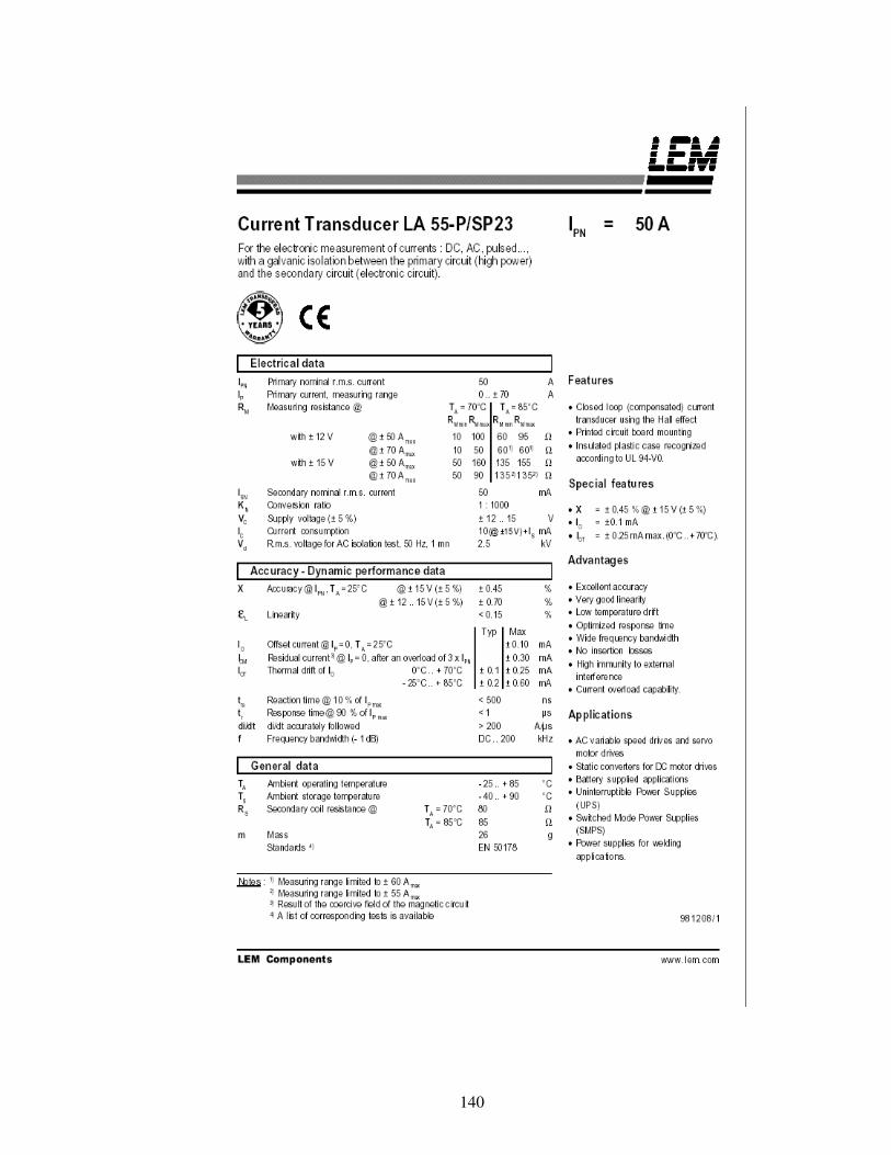
140

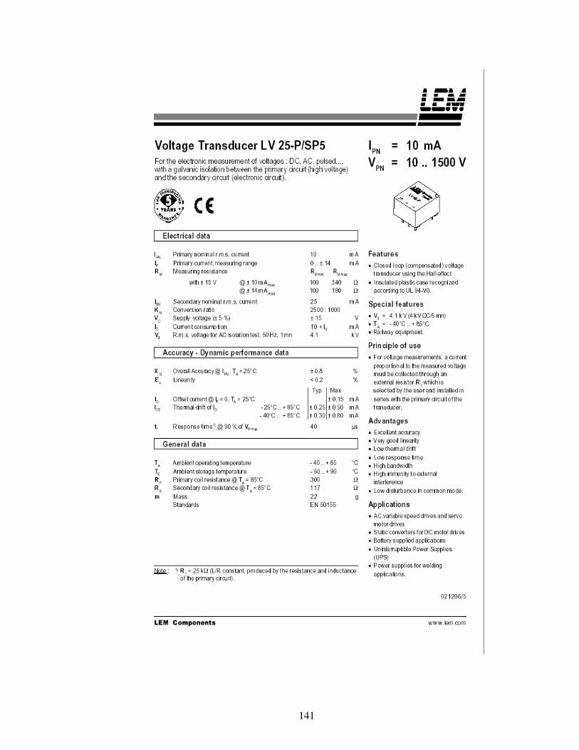
141

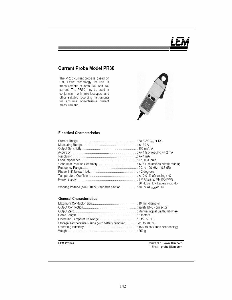
142

143

APPENDIX I

COMPARISON OF SPEED ESTIMATION METHODS

To verify the speed estimation methods, which are explained in Chapter3, 1.1,

2.2 and 4kW motors are driven with inverter. Measured currents and voltages are

logged by Trace program. Speed estimation methods are simulated in Matlab, by using

measured data. By this way, any error that may be introduced due to measurements is

taken into account these predictions. Speed estimation results are compared with

measured speed and motor simulation. Speed estimation results are shown in Table.I.1

to Table.I.24.

When motor is driven with inverter, a dc shift is seen on stator phase currents.

This dc shift worsens the estimation of power factor and rms value of stator current,

which are explained in Chapter 4. To verify the effect of dc shift on the stator current,

2.2 kW induction motor is driven with line voltage. Speed estimation results are

compared with measured speed and motor simulation. Speed estimation results are

shown in Table.I.25 and Table.I.26.

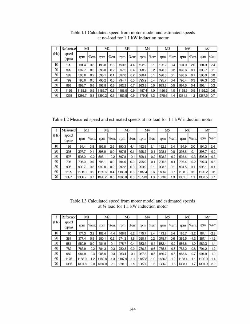
144

Table.I.1 Calculated speed from motor model and estimated speeds at no-load for 1.1 kW induction motor

rpm %err. rpm %err. rpm %err. rpm %err. rpm %err. rpm %err. rpm %err.

10 199 191.4 3.8 193.8 2.6 190.3 4.4 192.9 3.1 192.2 3.4 194.9 2.0 194.3 2.420 399 397.7 0.3 398.0 0.2 397.5 0.4 398.2 0.2 398.0 0.2 398.6 0.1 398.7 0.130 599 598.0 0.2 598.1 0.1 597.8 0.2 598.4 0.1 598.3 0.1 598.6 0.1 598.9 0.040 799 795.0 0.5 795.2 0.5 794.7 0.5 795.9 0.4 795.7 0.4 796.4 0.3 797.3 0.250 999 992.7 0.6 992.8 0.6 992.2 0.7 993.9 0.5 993.6 0.5 994.5 0.4 996.1 0.360 1199 1188.8 0.9 1189.7 0.8 1188.0 0.9 1187.4 1.0 1186.9 1.0 1188.6 0.9 1192.2 0.670 1398 1386.7 0.8 1390.2 0.6 1385.8 0.9 1379.3 1.3 1378.6 1.4 1381.3 1.2 1387.5 0.7

M5 M6f (Hz)

Reference speed (rpm)

M1 M2 M7M3 M4

Table.I.2 Measured speed and estimated speeds at no-load for 1.1 kW induction motor

rpm %err. rpm %err. rpm %err. rpm %err. rpm %err. rpm %err. rpm %err.

10 199 191.4 3.8 193.8 2.6 190.3 4.4 192.9 3.1 192.2 3.4 194.9 2.0 194.3 2.420 398 397.7 0.1 398.0 0.0 397.5 0.1 398.2 -0.1 398.1 0.0 398.6 -0.1 398.7 -0.230 597 598.0 -0.2 598.1 -0.2 597.8 -0.1 598.4 -0.2 598.3 -0.2 598.6 -0.3 598.9 -0.340 795 795.0 0.0 795.1 0.0 794.6 0.0 795.9 -0.1 795.6 -0.1 796.4 -0.2 797.3 -0.350 995 992.7 0.2 992.8 0.2 992.2 0.3 993.9 0.1 993.6 0.1 994.5 0.1 996.1 -0.160 1195 1188.8 0.5 1189.6 0.4 1188.0 0.6 1187.4 0.6 1186.8 0.7 1188.6 0.5 1192.2 0.270 1397 1386.7 0.7 1390.2 0.5 1385.8 0.8 1379.3 1.3 1378.6 1.3 1381.3 1.1 1387.5 0.7

M7f (Hz)

Measured speed (rpm)

M1 M2 M3 M4 M5 M6

Table.I.3 Calculated speed from motor model and estimated speeds at ¼ load for 1.1 kW induction motor

rpm %err. rpm %err. rpm %err. rpm %err. rpm %err. rpm %err. rpm %err.

10 180 174.3 3.2 182.4 -1.4 168.8 6.2 175.7 2.4 173.8 3.4 185.7 -3.2 184.1 -2.320 381 377.4 0.9 380.1 0.2 374.3 1.8 380.1 0.2 378.7 0.6 385.5 -1.2 387.1 -1.630 581 580.9 0.0 581.9 -0.1 578.7 0.4 583.5 -0.4 582.4 -0.2 586.6 -1.0 589.3 -1.440 782 783.9 -0.2 784.3 -0.3 782.3 0.0 786.3 -0.6 785.6 -0.5 788.2 -0.8 791.2 -1.250 982 984.9 -0.3 985.0 -0.3 983.4 -0.1 987.3 -0.5 986.7 -0.5 988.6 -0.7 991.9 -1.060 1175 1188.9 -1.2 1189.8 -1.3 1187.9 -1.1 1187.3 -1.0 1186.8 -1.0 1188.4 -1.1 1192.0 -1.470 1365 1391.8 -2.0 1394.0 -2.1 1391.1 -1.9 1387.2 -1.6 1386.8 -1.6 1388.1 -1.7 1391.9 -2.0

f (Hz)

Reference speed (rpm)

M1 M2 M3 M4 M5 M6 M7

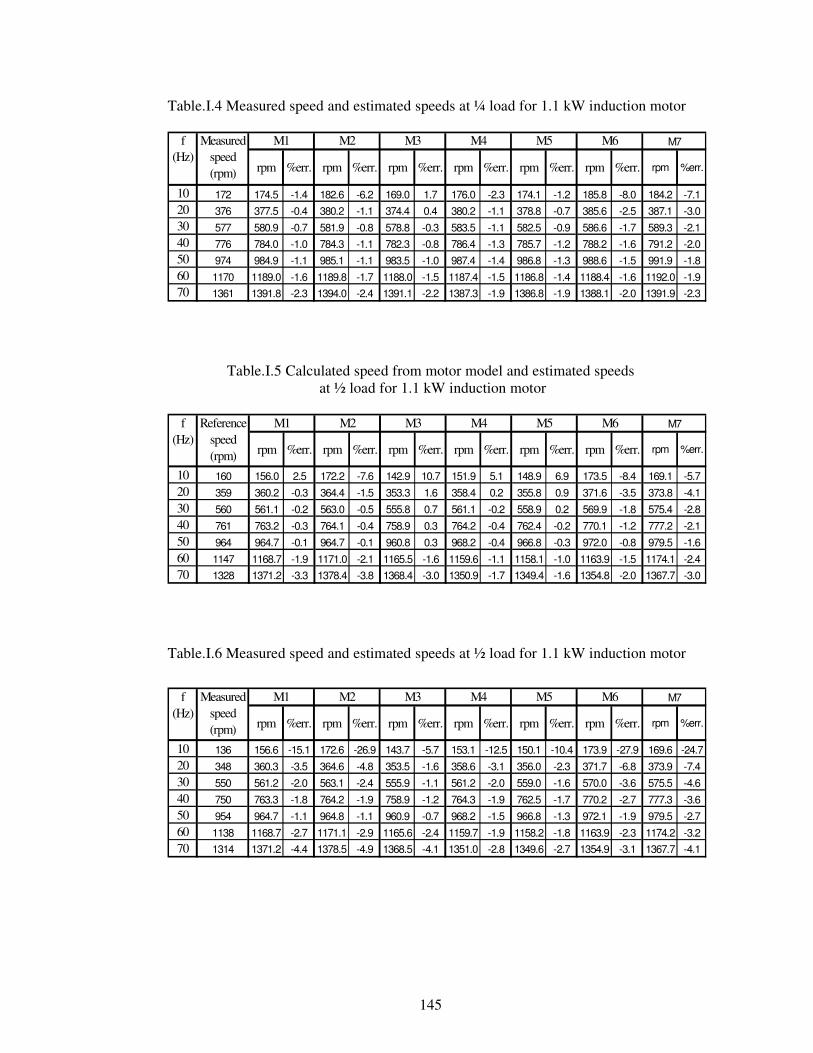
145

Table.I.4 Measured speed and estimated speeds at ¼ load for 1.1 kW induction motor

rpm %err. rpm %err. rpm %err. rpm %err. rpm %err. rpm %err. rpm %err.

10 172 174.5 -1.4 182.6 -6.2 169.0 1.7 176.0 -2.3 174.1 -1.2 185.8 -8.0 184.2 -7.120 376 377.5 -0.4 380.2 -1.1 374.4 0.4 380.2 -1.1 378.8 -0.7 385.6 -2.5 387.1 -3.030 577 580.9 -0.7 581.9 -0.8 578.8 -0.3 583.5 -1.1 582.5 -0.9 586.6 -1.7 589.3 -2.140 776 784.0 -1.0 784.3 -1.1 782.3 -0.8 786.4 -1.3 785.7 -1.2 788.2 -1.6 791.2 -2.050 974 984.9 -1.1 985.1 -1.1 983.5 -1.0 987.4 -1.4 986.8 -1.3 988.6 -1.5 991.9 -1.860 1170 1189.0 -1.6 1189.8 -1.7 1188.0 -1.5 1187.4 -1.5 1186.8 -1.4 1188.4 -1.6 1192.0 -1.970 1361 1391.8 -2.3 1394.0 -2.4 1391.1 -2.2 1387.3 -1.9 1386.8 -1.9 1388.1 -2.0 1391.9 -2.3

f (Hz)

Measured speed (rpm)

M1 M2 M3 M4 M5 M6 M7

Table.I.5 Calculated speed from motor model and estimated speeds at ½ load for 1.1 kW induction motor

rpm %err. rpm %err. rpm %err. rpm %err. rpm %err. rpm %err. rpm %err.

10 160 156.0 2.5 172.2 -7.6 142.9 10.7 151.9 5.1 148.9 6.9 173.5 -8.4 169.1 -5.720 359 360.2 -0.3 364.4 -1.5 353.3 1.6 358.4 0.2 355.8 0.9 371.6 -3.5 373.8 -4.130 560 561.1 -0.2 563.0 -0.5 555.8 0.7 561.1 -0.2 558.9 0.2 569.9 -1.8 575.4 -2.840 761 763.2 -0.3 764.1 -0.4 758.9 0.3 764.2 -0.4 762.4 -0.2 770.1 -1.2 777.2 -2.150 964 964.7 -0.1 964.7 -0.1 960.8 0.3 968.2 -0.4 966.8 -0.3 972.0 -0.8 979.5 -1.660 1147 1168.7 -1.9 1171.0 -2.1 1165.5 -1.6 1159.6 -1.1 1158.1 -1.0 1163.9 -1.5 1174.1 -2.470 1328 1371.2 -3.3 1378.4 -3.8 1368.4 -3.0 1350.9 -1.7 1349.4 -1.6 1354.8 -2.0 1367.7 -3.0

f (Hz)

Reference speed (rpm)

M1 M2 M3 M4 M5 M6 M7

Table.I.6 Measured speed and estimated speeds at ½ load for 1.1 kW induction motor

rpm %err. rpm %err. rpm %err. rpm %err. rpm %err. rpm %err. rpm %err.

10 136 156.6 -15.1 172.6 -26.9 143.7 -5.7 153.1 -12.5 150.1 -10.4 173.9 -27.9 169.6 -24.720 348 360.3 -3.5 364.6 -4.8 353.5 -1.6 358.6 -3.1 356.0 -2.3 371.7 -6.8 373.9 -7.430 550 561.2 -2.0 563.1 -2.4 555.9 -1.1 561.2 -2.0 559.0 -1.6 570.0 -3.6 575.5 -4.640 750 763.3 -1.8 764.2 -1.9 758.9 -1.2 764.3 -1.9 762.5 -1.7 770.2 -2.7 777.3 -3.650 954 964.7 -1.1 964.8 -1.1 960.9 -0.7 968.2 -1.5 966.8 -1.3 972.1 -1.9 979.5 -2.760 1138 1168.7 -2.7 1171.1 -2.9 1165.6 -2.4 1159.7 -1.9 1158.2 -1.8 1163.9 -2.3 1174.2 -3.270 1314 1371.2 -4.4 1378.5 -4.9 1368.5 -4.1 1351.0 -2.8 1349.6 -2.7 1354.9 -3.1 1367.7 -4.1

M6 M7M3 M4 M5f (Hz)

Measured speed (rpm)

M1 M2

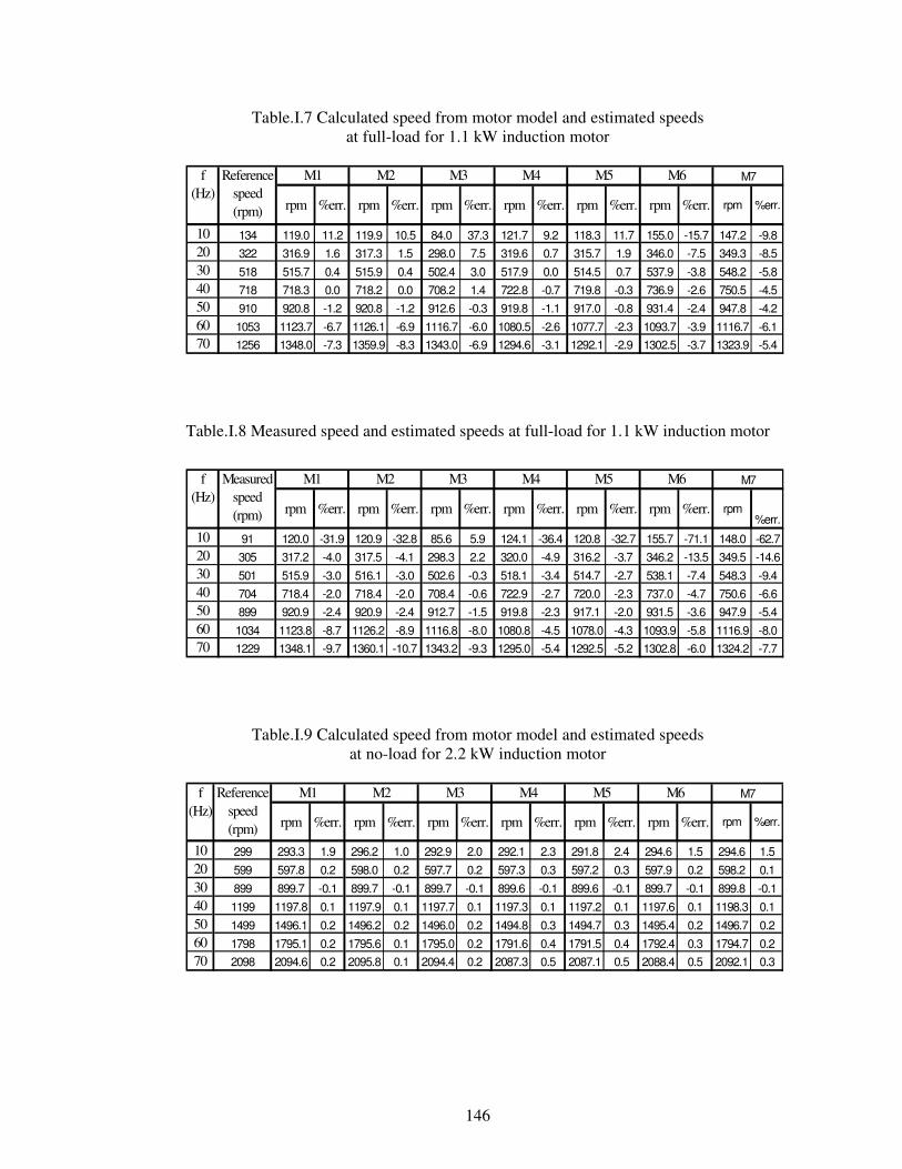
146

Table.I.7 Calculated speed from motor model and estimated speeds at full-load for 1.1 kW induction motor

rpm %err. rpm %err. rpm %err. rpm %err. rpm %err. rpm %err. rpm %err.

10 134 119.0 11.2 119.9 10.5 84.0 37.3 121.7 9.2 118.3 11.7 155.0 -15.7 147.2 -9.820 322 316.9 1.6 317.3 1.5 298.0 7.5 319.6 0.7 315.7 1.9 346.0 -7.5 349.3 -8.530 518 515.7 0.4 515.9 0.4 502.4 3.0 517.9 0.0 514.5 0.7 537.9 -3.8 548.2 -5.840 718 718.3 0.0 718.2 0.0 708.2 1.4 722.8 -0.7 719.8 -0.3 736.9 -2.6 750.5 -4.550 910 920.8 -1.2 920.8 -1.2 912.6 -0.3 919.8 -1.1 917.0 -0.8 931.4 -2.4 947.8 -4.260 1053 1123.7 -6.7 1126.1 -6.9 1116.7 -6.0 1080.5 -2.6 1077.7 -2.3 1093.7 -3.9 1116.7 -6.170 1256 1348.0 -7.3 1359.9 -8.3 1343.0 -6.9 1294.6 -3.1 1292.1 -2.9 1302.5 -3.7 1323.9 -5.4

M5M1 M2 M3 M4 M6 M7f (Hz)

Reference speed (rpm)

Table.I.8 Measured speed and estimated speeds at full-load for 1.1 kW induction motor

rpm %err. rpm %err. rpm %err. rpm %err. rpm %err. rpm %err. rpm%err.

10 91 120.0 -31.9 120.9 -32.8 85.6 5.9 124.1 -36.4 120.8 -32.7 155.7 -71.1 148.0 -62.720 305 317.2 -4.0 317.5 -4.1 298.3 2.2 320.0 -4.9 316.2 -3.7 346.2 -13.5 349.5 -14.630 501 515.9 -3.0 516.1 -3.0 502.6 -0.3 518.1 -3.4 514.7 -2.7 538.1 -7.4 548.3 -9.440 704 718.4 -2.0 718.4 -2.0 708.4 -0.6 722.9 -2.7 720.0 -2.3 737.0 -4.7 750.6 -6.650 899 920.9 -2.4 920.9 -2.4 912.7 -1.5 919.8 -2.3 917.1 -2.0 931.5 -3.6 947.9 -5.460 1034 1123.8 -8.7 1126.2 -8.9 1116.8 -8.0 1080.8 -4.5 1078.0 -4.3 1093.9 -5.8 1116.9 -8.070 1229 1348.1 -9.7 1360.1 -10.7 1343.2 -9.3 1295.0 -5.4 1292.5 -5.2 1302.8 -6.0 1324.2 -7.7

M7M3 M4 M5 M6f (Hz)

Measured speed (rpm)

M1 M2

Table.I.9 Calculated speed from motor model and estimated speeds at no-load for 2.2 kW induction motor

rpm %err. rpm %err. rpm %err. rpm %err. rpm %err. rpm %err. rpm %err.

10 299 293.3 1.9 296.2 1.0 292.9 2.0 292.1 2.3 291.8 2.4 294.6 1.5 294.6 1.520 599 597.8 0.2 598.0 0.2 597.7 0.2 597.3 0.3 597.2 0.3 597.9 0.2 598.2 0.130 899 899.7 -0.1 899.7 -0.1 899.7 -0.1 899.6 -0.1 899.6 -0.1 899.7 -0.1 899.8 -0.140 1199 1197.8 0.1 1197.9 0.1 1197.7 0.1 1197.3 0.1 1197.2 0.1 1197.6 0.1 1198.3 0.150 1499 1496.1 0.2 1496.2 0.2 1496.0 0.2 1494.8 0.3 1494.7 0.3 1495.4 0.2 1496.7 0.260 1798 1795.1 0.2 1795.6 0.1 1795.0 0.2 1791.6 0.4 1791.5 0.4 1792.4 0.3 1794.7 0.270 2098 2094.6 0.2 2095.8 0.1 2094.4 0.2 2087.3 0.5 2087.1 0.5 2088.4 0.5 2092.1 0.3

M7M3 M4 M5 M6f (Hz)

Reference speed (rpm)

M1 M2

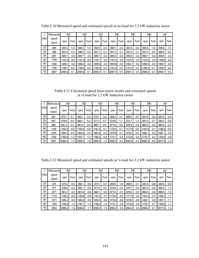
147

Table.I.10 Measured speed and estimated speeds at no-load for 2.2 kW induction motor

rpm %err. rpm %err. rpm %err. rpm %err. rpm %err. rpm %err. rpm %err.

10 299 293.3 1.9 296.2 1.0 292.9 2.0 292.1 2.3 291.8 2.4 294.6 1.5 294.6 1.520 598 597.8 0.0 598.0 0.0 597.7 0.1 597.3 0.1 597.2 0.1 597.9 0.0 598.2 0.030 897 899.7 -0.3 899.7 -0.3 899.7 -0.3 899.6 -0.3 899.6 -0.3 899.7 -0.3 899.8 -0.340 1194 1197.8 -0.3 1197.9 -0.3 1197.7 -0.3 1197.3 -0.3 1197.2 -0.3 1197.6 -0.3 1198.2 -0.450 1492 1496.1 -0.3 1496.2 -0.3 1495.9 -0.3 1494.8 -0.2 1494.7 -0.2 1495.3 -0.2 1496.7 -0.360 1795 1795.1 0.0 1795.6 0.0 1795.0 0.0 1791.6 0.2 1791.5 0.2 1792.4 0.1 1794.7 0.070 2097 2094.6 0.1 2095.8 0.1 2094.4 0.1 2087.3 0.5 2087.1 0.5 2088.4 0.4 2092.1 0.2

f (Hz)

Measured speed (rpm)

M1 M2 M3 M4 M5 M6 M7

Table.I.11 Calculated speed from motor model and estimated speeds at ¼ load for 2.2 kW induction motor

rpm %err. rpm %err. rpm %err. rpm %err. rpm %err. rpm %err. rpm %err.

10 281 275.1 2.1 282.1 -0.4 272.1 3.2 269.4 4.1 268.2 4.5 281.8 -0.3 281.9 -0.320 581 578.6 0.4 580.1 0.2 577.0 0.7 574.6 1.1 573.7 1.3 581.6 -0.1 584.3 -0.630 880 881.2 -0.1 881.9 -0.2 880.1 0.0 877.6 0.3 876.9 0.4 882.0 -0.2 885.9 -0.740 1180 1182.3 -0.2 1182.8 -0.2 1181.4 -0.1 1178.3 0.1 1177.8 0.2 1181.6 -0.1 1186.3 -0.550 1479 1484.2 -0.4 1484.6 -0.4 1483.4 -0.3 1479.8 -0.1 1479.3 0.0 1482.1 -0.2 1487.1 -0.560 1769 1785.8 -1.0 1787.1 -1.0 1785.2 -0.9 1774.1 -0.3 1773.6 -0.3 1776.7 -0.4 1783.6 -0.870 2057 2086.2 -1.4 2089.2 -1.6 2085.5 -1.4 2065.3 -0.4 2064.8 -0.4 2068.3 -0.5 2077.8 -1.0

M6 M7f (Hz)

Reference speed (rpm)

M1 M2 M3 M4 M5

Table.I.12 Measured speed and estimated speeds at ¼ load for 2.2 kW induction motor

rpm %err. rpm %err. rpm %err. rpm %err. rpm %err. rpm %err. rpm %err.

10 274 275.2 -0.4 282.1 -3.0 272.1 0.7 269.5 1.6 268.3 2.1 281.8 -2.8 282.0 -2.920 577 578.6 -0.3 580.1 -0.5 577.0 0.0 574.6 0.4 573.7 0.6 581.6 -0.8 584.3 -1.330 877 881.2 -0.5 881.9 -0.6 880.1 -0.3 877.6 -0.1 876.9 0.0 882.0 -0.6 885.9 -1.040 1173 1182.3 -0.8 1182.8 -0.8 1181.4 -0.7 1178.4 -0.5 1177.8 -0.4 1181.6 -0.7 1186.3 -1.150 1471 1484.2 -0.9 1484.6 -0.9 1483.5 -0.8 1479.8 -0.6 1479.4 -0.6 1482.1 -0.8 1487.1 -1.160 1764 1785.8 -1.2 1787.1 -1.3 1785.2 -1.2 1774.1 -0.6 1773.6 -0.5 1776.7 -0.7 1783.6 -1.170 2054 2086.2 -1.6 2089.2 -1.7 2085.5 -1.5 2065.3 -0.6 2064.8 -0.5 2068.3 -0.7 2077.8 -1.2

f (Hz)

Measured speed (rpm)

M1 M2 M3 M4 M5 M6 M7

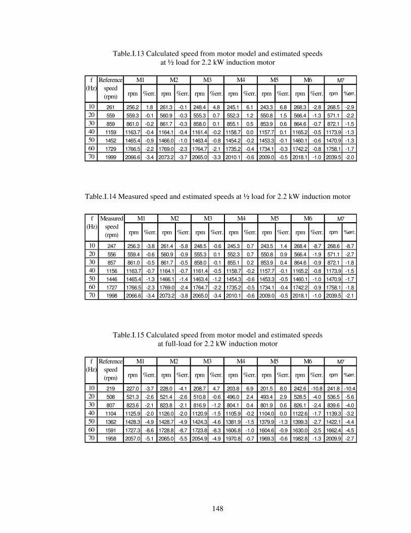
148

Table.I.13 Calculated speed from motor model and estimated speeds at ½ load for 2.2 kW induction motor

rpm %err. rpm %err. rpm %err. rpm %err. rpm %err. rpm %err. rpm %err.

10 261 256.2 1.8 261.3 -0.1 248.4 4.8 245.1 6.1 243.3 6.8 268.3 -2.8 268.5 -2.920 559 559.3 -0.1 560.9 -0.3 555.3 0.7 552.3 1.2 550.8 1.5 566.4 -1.3 571.1 -2.230 859 861.0 -0.2 861.7 -0.3 858.0 0.1 855.1 0.5 853.9 0.6 864.6 -0.7 872.1 -1.540 1159 1163.7 -0.4 1164.1 -0.4 1161.4 -0.2 1158.7 0.0 1157.7 0.1 1165.2 -0.5 1173.9 -1.350 1452 1465.4 -0.9 1466.0 -1.0 1463.4 -0.8 1454.2 -0.2 1453.3 -0.1 1460.1 -0.6 1470.9 -1.360 1729 1766.5 -2.2 1769.0 -2.3 1764.7 -2.1 1735.2 -0.4 1734.1 -0.3 1742.2 -0.8 1758.1 -1.770 1999 2066.6 -3.4 2073.2 -3.7 2065.0 -3.3 2010.1 -0.6 2009.0 -0.5 2018.1 -1.0 2039.5 -2.0

M6 M7f (Hz)

Reference speed (rpm)

M1 M2 M3 M4 M5

Table.I.14 Measured speed and estimated speeds at ½ load for 2.2 kW induction motor

rpm %err. rpm %err. rpm %err. rpm %err. rpm %err. rpm %err. rpm %err.

10 247 256.3 -3.8 261.4 -5.8 248.5 -0.6 245.3 0.7 243.5 1.4 268.4 -8.7 268.6 -8.720 556 559.4 -0.6 560.9 -0.9 555.3 0.1 552.3 0.7 550.8 0.9 566.4 -1.9 571.1 -2.730 857 861.0 -0.5 861.7 -0.5 858.0 -0.1 855.1 0.2 853.9 0.4 864.6 -0.9 872.1 -1.840 1156 1163.7 -0.7 1164.1 -0.7 1161.4 -0.5 1158.7 -0.2 1157.7 -0.1 1165.2 -0.8 1173.9 -1.550 1446 1465.4 -1.3 1466.1 -1.4 1463.4 -1.2 1454.3 -0.6 1453.3 -0.5 1460.1 -1.0 1470.9 -1.760 1727 1766.5 -2.3 1769.0 -2.4 1764.7 -2.2 1735.2 -0.5 1734.1 -0.4 1742.2 -0.9 1758.1 -1.870 1998 2066.6 -3.4 2073.2 -3.8 2065.0 -3.4 2010.1 -0.6 2009.0 -0.5 2018.1 -1.0 2039.5 -2.1

f (Hz)

Measured speed (rpm)

M1 M2 M3 M4 M5 M6 M7

Table.I.15 Calculated speed from motor model and estimated speeds at full-load for 2.2 kW induction motor

rpm %err. rpm %err. rpm %err. rpm %err. rpm %err. rpm %err. rpm %err.

10 219 227.0 -3.7 228.0 -4.1 208.7 4.7 203.8 6.9 201.5 8.0 242.6 -10.8 241.8 -10.420 508 521.3 -2.6 521.4 -2.6 510.8 -0.6 496.0 2.4 493.4 2.9 528.5 -4.0 536.5 -5.630 807 823.6 -2.1 823.8 -2.1 816.9 -1.2 804.1 0.4 801.9 0.6 826.1 -2.4 839.6 -4.040 1104 1125.9 -2.0 1126.0 -2.0 1120.9 -1.5 1105.9 -0.2 1104.0 0.0 1122.6 -1.7 1139.3 -3.250 1362 1428.3 -4.9 1428.7 -4.9 1424.3 -4.6 1381.9 -1.5 1379.9 -1.3 1399.3 -2.7 1422.1 -4.460 1591 1727.3 -8.6 1728.8 -8.7 1723.8 -8.3 1606.8 -1.0 1604.6 -0.9 1630.0 -2.5 1662.4 -4.570 1958 2057.0 -5.1 2065.0 -5.5 2054.9 -4.9 1970.8 -0.7 1969.3 -0.6 1982.8 -1.3 2009.9 -2.7

M6 M7f (Hz)

Reference speed (rpm)

M1 M2 M3 M4 M5

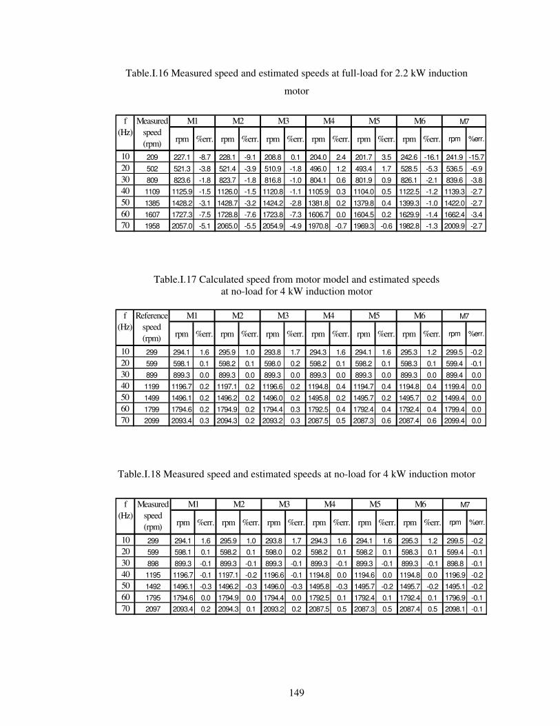
149

Table.I.16 Measured speed and estimated speeds at full-load for 2.2 kW induction

motor

rpm %err. rpm %err. rpm %err. rpm %err. rpm %err. rpm %err. rpm %err.

10 209 227.1 -8.7 228.1 -9.1 208.8 0.1 204.0 2.4 201.7 3.5 242.6 -16.1 241.9 -15.720 502 521.3 -3.8 521.4 -3.9 510.9 -1.8 496.0 1.2 493.4 1.7 528.5 -5.3 536.5 -6.930 809 823.6 -1.8 823.7 -1.8 816.8 -1.0 804.1 0.6 801.9 0.9 826.1 -2.1 839.6 -3.840 1109 1125.9 -1.5 1126.0 -1.5 1120.8 -1.1 1105.9 0.3 1104.0 0.5 1122.5 -1.2 1139.3 -2.750 1385 1428.2 -3.1 1428.7 -3.2 1424.2 -2.8 1381.8 0.2 1379.8 0.4 1399.3 -1.0 1422.0 -2.760 1607 1727.3 -7.5 1728.8 -7.6 1723.8 -7.3 1606.7 0.0 1604.5 0.2 1629.9 -1.4 1662.4 -3.470 1958 2057.0 -5.1 2065.0 -5.5 2054.9 -4.9 1970.8 -0.7 1969.3 -0.6 1982.8 -1.3 2009.9 -2.7

f (Hz)

Measured speed (rpm)

M1 M2 M7M3 M4 M5 M6

Table.I.17 Calculated speed from motor model and estimated speeds at no-load for 4 kW induction motor

rpm %err. rpm %err. rpm %err. rpm %err. rpm %err. rpm %err. rpm %err.

10 299 294.1 1.6 295.9 1.0 293.8 1.7 294.3 1.6 294.1 1.6 295.3 1.2 299.5 -0.220 599 598.1 0.1 598.2 0.1 598.0 0.2 598.2 0.1 598.2 0.1 598.3 0.1 599.4 -0.130 899 899.3 0.0 899.3 0.0 899.3 0.0 899.3 0.0 899.3 0.0 899.3 0.0 899.4 0.040 1199 1196.7 0.2 1197.1 0.2 1196.6 0.2 1194.8 0.4 1194.7 0.4 1194.8 0.4 1199.4 0.050 1499 1496.1 0.2 1496.2 0.2 1496.0 0.2 1495.8 0.2 1495.7 0.2 1495.7 0.2 1499.4 0.060 1799 1794.6 0.2 1794.9 0.2 1794.4 0.3 1792.5 0.4 1792.4 0.4 1792.4 0.4 1799.4 0.070 2099 2093.4 0.3 2094.3 0.2 2093.2 0.3 2087.5 0.5 2087.3 0.6 2087.4 0.6 2099.4 0.0

f (Hz)

Reference speed (rpm)

M1 M2 M3 M4 M5 M6 M7

Table.I.18 Measured speed and estimated speeds at no-load for 4 kW induction motor

rpm %err. rpm %err. rpm %err. rpm %err. rpm %err. rpm %err. rpm %err.

10 299 294.1 1.6 295.9 1.0 293.8 1.7 294.3 1.6 294.1 1.6 295.3 1.2 299.5 -0.220 599 598.1 0.1 598.2 0.1 598.0 0.2 598.2 0.1 598.2 0.1 598.3 0.1 599.4 -0.130 898 899.3 -0.1 899.3 -0.1 899.3 -0.1 899.3 -0.1 899.3 -0.1 899.3 -0.1 898.8 -0.140 1195 1196.7 -0.1 1197.1 -0.2 1196.6 -0.1 1194.8 0.0 1194.6 0.0 1194.8 0.0 1196.9 -0.250 1492 1496.1 -0.3 1496.2 -0.3 1496.0 -0.3 1495.8 -0.3 1495.7 -0.2 1495.7 -0.2 1495.1 -0.260 1795 1794.6 0.0 1794.9 0.0 1794.4 0.0 1792.5 0.1 1792.4 0.1 1792.4 0.1 1796.9 -0.170 2097 2093.4 0.2 2094.3 0.1 2093.2 0.2 2087.5 0.5 2087.3 0.5 2087.4 0.5 2098.1 -0.1

M7M3 M4 M5 M6f (Hz)

Measured speed (rpm)

M1 M2

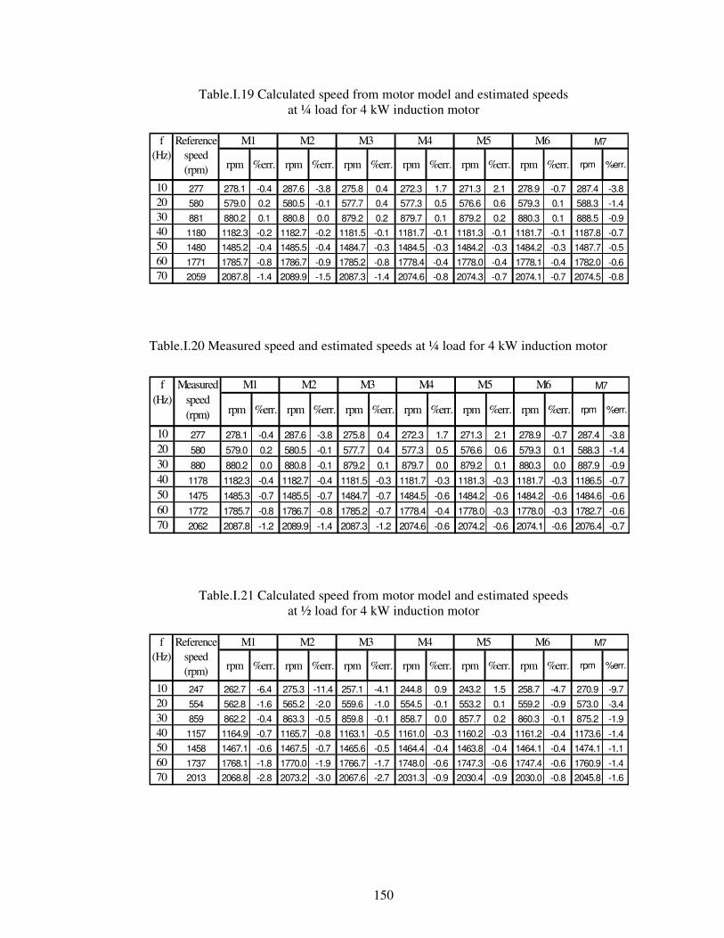
150

Table.I.19 Calculated speed from motor model and estimated speeds at ¼ load for 4 kW induction motor

rpm %err. rpm %err. rpm %err. rpm %err. rpm %err. rpm %err. rpm %err.

10 277 278.1 -0.4 287.6 -3.8 275.8 0.4 272.3 1.7 271.3 2.1 278.9 -0.7 287.4 -3.820 580 579.0 0.2 580.5 -0.1 577.7 0.4 577.3 0.5 576.6 0.6 579.3 0.1 588.3 -1.430 881 880.2 0.1 880.8 0.0 879.2 0.2 879.7 0.1 879.2 0.2 880.3 0.1 888.5 -0.940 1180 1182.3 -0.2 1182.7 -0.2 1181.5 -0.1 1181.7 -0.1 1181.3 -0.1 1181.7 -0.1 1187.8 -0.750 1480 1485.2 -0.4 1485.5 -0.4 1484.7 -0.3 1484.5 -0.3 1484.2 -0.3 1484.2 -0.3 1487.7 -0.560 1771 1785.7 -0.8 1786.7 -0.9 1785.2 -0.8 1778.4 -0.4 1778.0 -0.4 1778.1 -0.4 1782.0 -0.670 2059 2087.8 -1.4 2089.9 -1.5 2087.3 -1.4 2074.6 -0.8 2074.3 -0.7 2074.1 -0.7 2074.5 -0.8

f (Hz)

Reference speed (rpm)

M1 M2 M3 M4 M5 M6 M7

Table.I.20 Measured speed and estimated speeds at ¼ load for 4 kW induction motor

rpm %err. rpm %err. rpm %err. rpm %err. rpm %err. rpm %err. rpm %err.

10 277 278.1 -0.4 287.6 -3.8 275.8 0.4 272.3 1.7 271.3 2.1 278.9 -0.7 287.4 -3.820 580 579.0 0.2 580.5 -0.1 577.7 0.4 577.3 0.5 576.6 0.6 579.3 0.1 588.3 -1.430 880 880.2 0.0 880.8 -0.1 879.2 0.1 879.7 0.0 879.2 0.1 880.3 0.0 887.9 -0.940 1178 1182.3 -0.4 1182.7 -0.4 1181.5 -0.3 1181.7 -0.3 1181.3 -0.3 1181.7 -0.3 1186.5 -0.750 1475 1485.3 -0.7 1485.5 -0.7 1484.7 -0.7 1484.5 -0.6 1484.2 -0.6 1484.2 -0.6 1484.6 -0.660 1772 1785.7 -0.8 1786.7 -0.8 1785.2 -0.7 1778.4 -0.4 1778.0 -0.3 1778.0 -0.3 1782.7 -0.670 2062 2087.8 -1.2 2089.9 -1.4 2087.3 -1.2 2074.6 -0.6 2074.2 -0.6 2074.1 -0.6 2076.4 -0.7

M6 M7f (Hz)

Measured speed (rpm)

M1 M2 M3 M4 M5

Table.I.21 Calculated speed from motor model and estimated speeds at ½ load for 4 kW induction motor

rpm %err. rpm %err. rpm %err. rpm %err. rpm %err. rpm %err. rpm %err.

10 247 262.7 -6.4 275.3 -11.4 257.1 -4.1 244.8 0.9 243.2 1.5 258.7 -4.7 270.9 -9.720 554 562.8 -1.6 565.2 -2.0 559.6 -1.0 554.5 -0.1 553.2 0.1 559.2 -0.9 573.0 -3.430 859 862.2 -0.4 863.3 -0.5 859.8 -0.1 858.7 0.0 857.7 0.2 860.3 -0.1 875.2 -1.940 1157 1164.9 -0.7 1165.7 -0.8 1163.1 -0.5 1161.0 -0.3 1160.2 -0.3 1161.2 -0.4 1173.6 -1.450 1458 1467.1 -0.6 1467.5 -0.7 1465.6 -0.5 1464.4 -0.4 1463.8 -0.4 1464.1 -0.4 1474.1 -1.160 1737 1768.1 -1.8 1770.0 -1.9 1766.7 -1.7 1748.0 -0.6 1747.3 -0.6 1747.4 -0.6 1760.9 -1.470 2013 2068.8 -2.8 2073.2 -3.0 2067.6 -2.7 2031.3 -0.9 2030.4 -0.9 2030.0 -0.8 2045.8 -1.6

f (Hz)

Reference speed (rpm)

M1 M2 M3 M4 M5 M6 M7

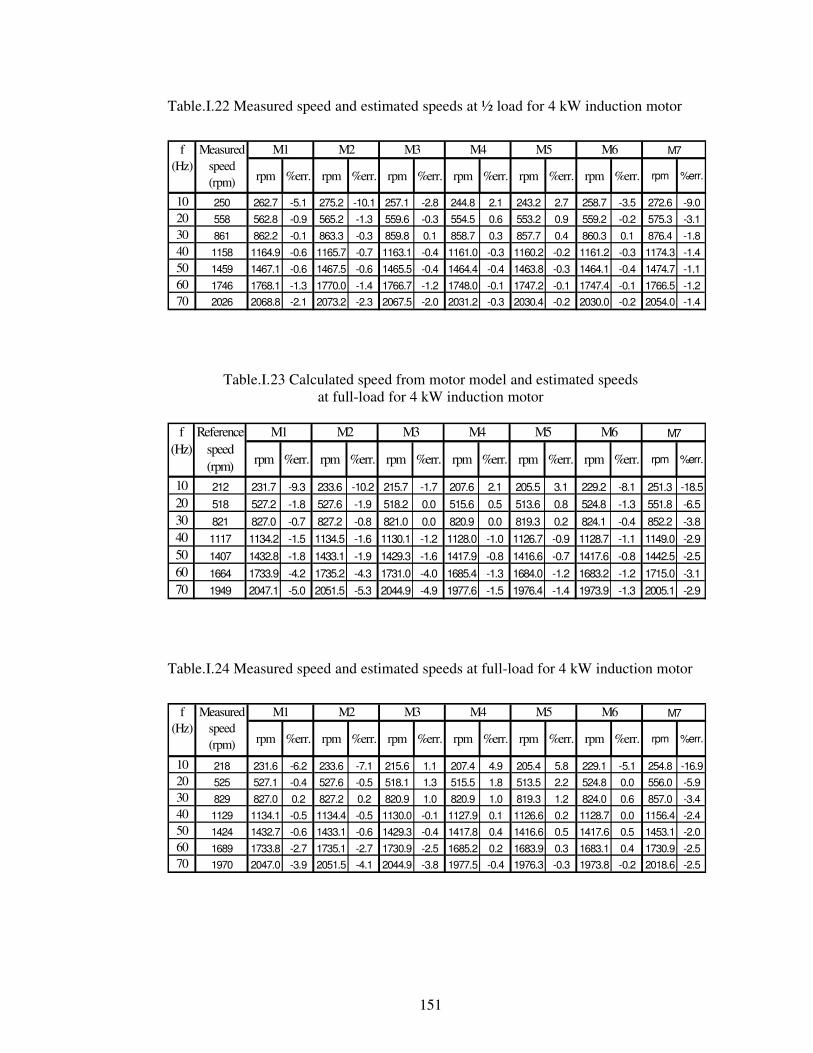
151

Table.I.22 Measured speed and estimated speeds at ½ load for 4 kW induction motor

rpm %err. rpm %err. rpm %err. rpm %err. rpm %err. rpm %err. rpm %err.

10 250 262.7 -5.1 275.2 -10.1 257.1 -2.8 244.8 2.1 243.2 2.7 258.7 -3.5 272.6 -9.020 558 562.8 -0.9 565.2 -1.3 559.6 -0.3 554.5 0.6 553.2 0.9 559.2 -0.2 575.3 -3.130 861 862.2 -0.1 863.3 -0.3 859.8 0.1 858.7 0.3 857.7 0.4 860.3 0.1 876.4 -1.840 1158 1164.9 -0.6 1165.7 -0.7 1163.1 -0.4 1161.0 -0.3 1160.2 -0.2 1161.2 -0.3 1174.3 -1.450 1459 1467.1 -0.6 1467.5 -0.6 1465.5 -0.4 1464.4 -0.4 1463.8 -0.3 1464.1 -0.4 1474.7 -1.160 1746 1768.1 -1.3 1770.0 -1.4 1766.7 -1.2 1748.0 -0.1 1747.2 -0.1 1747.4 -0.1 1766.5 -1.270 2026 2068.8 -2.1 2073.2 -2.3 2067.5 -2.0 2031.2 -0.3 2030.4 -0.2 2030.0 -0.2 2054.0 -1.4

M6 M7f (Hz)

Measured speed (rpm)

M1 M2 M3 M4 M5

Table.I.23 Calculated speed from motor model and estimated speeds at full-load for 4 kW induction motor

rpm %err. rpm %err. rpm %err. rpm %err. rpm %err. rpm %err. rpm %err.

10 212 231.7 -9.3 233.6 -10.2 215.7 -1.7 207.6 2.1 205.5 3.1 229.2 -8.1 251.3 -18.520 518 527.2 -1.8 527.6 -1.9 518.2 0.0 515.6 0.5 513.6 0.8 524.8 -1.3 551.8 -6.530 821 827.0 -0.7 827.2 -0.8 821.0 0.0 820.9 0.0 819.3 0.2 824.1 -0.4 852.2 -3.840 1117 1134.2 -1.5 1134.5 -1.6 1130.1 -1.2 1128.0 -1.0 1126.7 -0.9 1128.7 -1.1 1149.0 -2.950 1407 1432.8 -1.8 1433.1 -1.9 1429.3 -1.6 1417.9 -0.8 1416.6 -0.7 1417.6 -0.8 1442.5 -2.560 1664 1733.9 -4.2 1735.2 -4.3 1731.0 -4.0 1685.4 -1.3 1684.0 -1.2 1683.2 -1.2 1715.0 -3.170 1949 2047.1 -5.0 2051.5 -5.3 2044.9 -4.9 1977.6 -1.5 1976.4 -1.4 1973.9 -1.3 2005.1 -2.9

f (Hz)

Reference speed (rpm)

M1 M2 M3 M4 M5 M6 M7

Table.I.24 Measured speed and estimated speeds at full-load for 4 kW induction motor

rpm %err. rpm %err. rpm %err. rpm %err. rpm %err. rpm %err. rpm %err.

10 218 231.6 -6.2 233.6 -7.1 215.6 1.1 207.4 4.9 205.4 5.8 229.1 -5.1 254.8 -16.920 525 527.1 -0.4 527.6 -0.5 518.1 1.3 515.5 1.8 513.5 2.2 524.8 0.0 556.0 -5.930 829 827.0 0.2 827.2 0.2 820.9 1.0 820.9 1.0 819.3 1.2 824.0 0.6 857.0 -3.440 1129 1134.1 -0.5 1134.4 -0.5 1130.0 -0.1 1127.9 0.1 1126.6 0.2 1128.7 0.0 1156.4 -2.450 1424 1432.7 -0.6 1433.1 -0.6 1429.3 -0.4 1417.8 0.4 1416.6 0.5 1417.6 0.5 1453.1 -2.060 1689 1733.8 -2.7 1735.1 -2.7 1730.9 -2.5 1685.2 0.2 1683.9 0.3 1683.1 0.4 1730.9 -2.570 1970 2047.0 -3.9 2051.5 -4.1 2044.9 -3.8 1977.5 -0.4 1976.3 -0.3 1973.8 -0.2 2018.6 -2.5

M6 M7f (Hz)

Measured speed (rpm)

M1 M2 M3 M4 M5

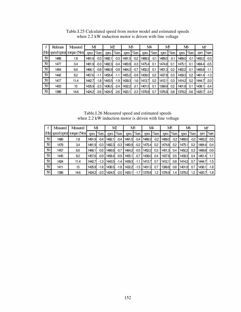
152

rpm %err. rpm %err. rpm %err. rpm %err. rpm %err. rpm %err. rpm %err.

50 1488 1.8 1491.9 -0.3 1492.1 -0.3 1491.5 -0.2 1489.3 -0.1 1489.0 -0.1 1489.0 -0.1 1493.2 -0.3

50 1477 3.4 1481.9 -0.3 1482.3 -0.4 1480.9 -0.3 1475.4 0.1 1474.8 0.1 1475.1 0.1 1484.4 -0.550 1454 6.6 1466.1 -0.8 1466.9 -0.9 1464.2 -0.7 1452.2 0.1 1451.3 0.2 1452.2 0.1 1469.8 -1.1

50 1442 8.2 1457.6 -1.1 1458.4 -1.1 1455.2 -0.9 1439.0 0.2 1437.8 0.3 1439.3 0.2 1461.4 -1.350 1417 11.4 1442.7 -1.8 1443.5 -1.9 1439.3 -1.6 1413.7 0.2 1412.1 0.3 1414.2 0.2 1444.7 -2.0

50 1403 13 1435.9 -2.3 1436.5 -2.4 1432.2 -2.1 1401.5 0.1 1399.9 0.2 1401.8 0.1 1436.1 -2.450 1388 14.6 1424.2 -2.6 1424.5 -2.6 1420.1 -2.3 1378.8 0.7 1376.9 0.8 1379.2 0.6 1420.7 -2.4

M6 M7M2 M3 M4 M5f (Hz)

Referans speed (rpm)

Measured torque (Nm)

M1

rpm %err. rpm %err. rpm %err. rpm %err. rpm %err. rpm %err. rpm %err.

50 1486 1.8 1491.9 -0.4 1492.1 -0.4 1491.5 -0.4 1489.3 -0.2 1489.0 -0.2 1489.0 -0.2 1493.2 -0.5

50 1478 3.4 1481.9 -0.3 1482.3 -0.3 1480.9 -0.2 1475.4 0.2 1474.8 0.2 1475.1 0.2 1484.4 -0.4

50 1457 6.6 1466.1 -0.6 1466.8 -0.7 1464.2 -0.5 1452.2 0.3 1451.3 0.4 1452.2 0.3 1469.8 -0.950 1445 8.2 1457.6 -0.9 1458.4 -0.9 1455.1 -0.7 1439.0 0.4 1437.8 0.5 1439.3 0.4 1461.4 -1.1

50 1424 11.4 1442.7 -1.3 1443.5 -1.4 1439.3 -1.1 1413.7 0.7 1412.1 0.8 1414.2 0.7 1444.7 -1.5

50 1411 13 1435.9 -1.8 1436.5 -1.8 1432.2 -1.5 1401.5 0.7 1399.8 0.8 1401.8 0.7 1436.1 -1.850 1396 14.6 1424.2 -2.0 1424.5 -2.0 1420.1 -1.7 1378.8 1.2 1376.9 1.4 1379.2 1.2 1420.7 -1.8

M7Measured torque (Nm)

M3 M4 M5 M6f (Hz)

Measured speed (rpm)

M1 M2

Table.I.25 Calculated speed from motor model and estimated speeds when 2.2 kW induction motor is driven with line voltage

Table.I.26 Measured speed and estimated speeds when 2.2 kW induction motor is driven with line voltage

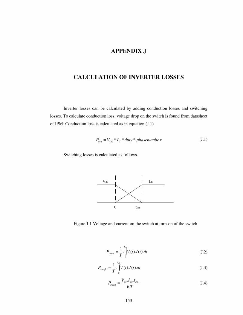
153

rphasenumbedutyIVP CCEcon ***=

=ont

swon dttItVT

P0

).().(.1

TtIV

P ondcdcswon .6

..=

=offt

swoff dttItVT

P0

).().(.1

APPENDIX J

CALCULATION OF INVERTER LOSSES

Inverter losses can be calculated by adding conduction losses and switching

losses. To calculate conduction loss, voltage drop on the switch is found from datasheet

of IPM. Conduction loss is calculated as in equation (J.1).

(J.1)

Switching losses is calculated as follows.

Vdc Idc

0 ton

Figure.J.1 Voltage and current on the switch at turn-on of the switch

(J.2)

(J.3)

(J.4)

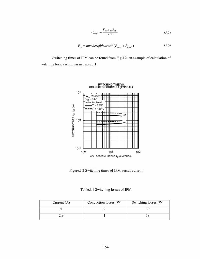
154

T

tIVP offdcdc

swoff .6

..=

)(* swoffswonsw PPasesnumberofphP +=

(J.5)

(J.6)

Switching times of IPM can be found from Fig.J.2. an example of calculation of

witching losses is shown in Table.J.1.

Figure.J.2 Switching times of IPM versus current

Table.J.1 Switching losses of IPM

Current (A) Conduction losses (W) Switching losses (W)

5 2 30

2.9 1 18

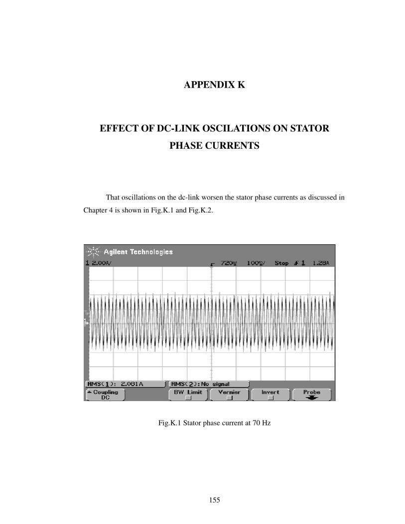
155

APPENDIX K

EFFECT OF DC-LINK OSCILATIONS ON STATOR

PHASE CURRENTS

That oscillations on the dc-link worsen the stator phase currents as discussed in

Chapter 4 is shown in Fig.K.1 and Fig.K.2.

Fig.K.1 Stator phase current at 70 Hz

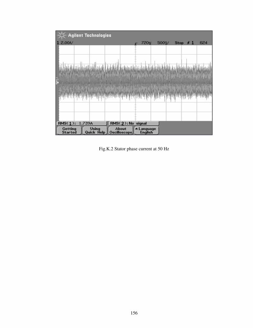
156

Fig.K.2 Stator phase current at 50 Hz