Embed Size (px)
Citation preview
Parallel Simulation of Verilog HDL Designs
DUAL DEGREE DISSERTATION
Submitted in partial ful�llment of
the requirements for the degree of
Bachelor of Technology(Electrical Engineering)
and
Master of Technology(Microelectronics)
by
Kumar Akarsh(08D07043)
Under the guidance of
Prof. Sachin B. Patkar
Department of Electrical EngineeringIndian Institute of Technology, Bombay.
June 2013

Declaration
I declare that this written submission represents my ideas in my own words
and where others' ideas or words have been included, I have adequately cited and
referenced the original sources. I also declare that I have adhered to all principles
of academic honesty and integrity and have not misrepresented or fabricated or
falsi�ed any idea/data/fact/source in my submission. I understand that any vio-
lation of the above will be cause for disciplinary action by the Institute and can
also evoke penal action from the sources which have thus not been properly cited
or from whom proper permission has not been taken when needed.
Kumar Akarsh
08D07043
Date: 24/06/2013
Place: IIT Bombay, Mumbai
i
Acknowledgement
I would really like to thank my guide and supervisor, Prof. Sachin Patkar, for
the guidance and support he has provided me throughout. The con�dence he has
shown me has de�nitely boosted my morale and has �lled me with a sence of self-
con�dence.
I would also like to thank my colleague, Dilawar Singh and Vinay Kumar(currently
pursuing PhD, HPC lab, EE, IITB), who has helped me in various ways, whenever
I was stuck at any point, throughout the project.
Also, I want to extend my thanks to Satwik Kottur (3rd year, EE, IITB), for our
productive discussions and his programming support for multiple parts.
Brainstorming sessions over each other's projects with my friends, Samyak Jaroli,
Uttam Sikaria and Sanket Diwale have been very productive and insightful. I
would really like to thank them too.
Last but not least, I would really like to thank my parents. They were there with
me to support me morally at all stages of my life.
�
Kumar Akarsh
ii
Abstract
Simulation of hardware designs forms a major part of the work done before synthe-
sis. It consumes a lot of time and cost if the designs are large enough. Reducing
this time and cost is highly desirable for research groups and even more by the
industries. Also, it involves a lot of steps which have to be taken care of in a
serial manner. So, automation of complete design �ow from hardware design to
its synthesis is also desirable. Moreover, sometimes we design hardware on one
platform and later want to use it on several other platforms. A tool which provides
such functionality of easy multi-platform conversion, will also be useful for such
applications.
This project tries to resolve all three problems. The main focus is on paralleliz-
ing the simulation of hardware as much as possible without any time or resource
con�ict. Single clock structural/behavioural hardware designs are converted to
standard XML structure for multi-platform applications. This structure can eas-
ily be parsed in any high level language using standard libraries. It is then analyzed
the in the HL language, after which we try to algorithmically identify the compo-
nents which can be parallelized. The design is then partitioned into such smaller
functional components. Individual threads are launched for simulation of each of
these components, on a multi-core platform. The time involved gets suppressed
multi-fold, depending upon the number of cores used. With the recent advance-
ments in the �eld of High performance computing, such as many-core processors,
we can exploit its full-�edged power to make Hardware simulation extremely fast
and e�cient.
Keywords: Hardware Simulation, Parallel processing, High level analysis, Parti-
tioning, Many-core processors, Hardware software co-design
iii
Contents
Abstract iii
1 Introduction 1
1.1 Project Objectives . . . . . . . . . . . . . . . . . . . . . . . . . . . 1
1.2 Project Roadmap . . . . . . . . . . . . . . . . . . . . . . . . . . . . 1
2 Overview of High level analysis model 3
3 Verilog HDL's constructs supported 6
3.1 wires and regs . . . . . . . . . . . . . . . . . . . . . . . . . . . . . 6
3.2 Independent hardware blocks . . . . . . . . . . . . . . . . . . . . . 7
3.3 Decision structures (MUXs) . . . . . . . . . . . . . . . . . . . . . . 7
3.4 Additional support features . . . . . . . . . . . . . . . . . . . . . . 7
3.5 Ambiguity resolving features . . . . . . . . . . . . . . . . . . . . . . 8
4 Structure of the high level model 11
4.1 ports . . . . . . . . . . . . . . . . . . . . . . . . . . . . . . . . . . . 11
4.2 declarations . . . . . . . . . . . . . . . . . . . . . . . . . . . . . . . 11
4.2.1 list of registers . . . . . . . . . . . . . . . . . . . . . . . . . 12
4.2.2 list of wires . . . . . . . . . . . . . . . . . . . . . . . . . . . 12
4.2.3 list of memories . . . . . . . . . . . . . . . . . . . . . . . . . 12
4.3 statements . . . . . . . . . . . . . . . . . . . . . . . . . . . . . . . . 12
4.3.1 assign statements . . . . . . . . . . . . . . . . . . . . . . . 12
4.3.2 initial block . . . . . . . . . . . . . . . . . . . . . . . . . . 12
4.3.3 always blocks . . . . . . . . . . . . . . . . . . . . . . . . . . 13
iv
5 Details of implementation 14
5.1 Classes used . . . . . . . . . . . . . . . . . . . . . . . . . . . . . . . 14
5.1.1 Class mainModule . . . . . . . . . . . . . . . . . . . . . . . . 14
5.1.2 Ports . . . . . . . . . . . . . . . . . . . . . . . . . . . . . . . 15
5.1.3 Declarations . . . . . . . . . . . . . . . . . . . . . . . . . . . 16
5.1.4 Statements . . . . . . . . . . . . . . . . . . . . . . . . . . . 17
6 Validation of the parsed results 22
7 Analysis of parsed Verilog design 24
7.1 Construction of graph . . . . . . . . . . . . . . . . . . . . . . . . . 24
7.1.1 Registers . . . . . . . . . . . . . . . . . . . . . . . . . . . . . 25
7.1.2 Wires . . . . . . . . . . . . . . . . . . . . . . . . . . . . . . 26
7.1.3 Continuous Assignments . . . . . . . . . . . . . . . . . . . . 26
7.1.4 Always blocks . . . . . . . . . . . . . . . . . . . . . . . . . . 26
7.1.5 Connecting blocking variables . . . . . . . . . . . . . . . . . 28
7.1.6 Drawing �nal edges . . . . . . . . . . . . . . . . . . . . . . . 29
7.1.7 Removing vertices . . . . . . . . . . . . . . . . . . . . . . . . 31
8 Extraction of Cones 32
9 Visualization of the graphs constructed 34
9.1 Digital design and other information stored in graphs . . . . . . . . 34
9.2 Parent Graph visual scheme . . . . . . . . . . . . . . . . . . . . . . 37
9.3 Cone Graph visual scheme . . . . . . . . . . . . . . . . . . . . . . . 37
10 Conversion of cones to C threads 38
10.1 Cones to single assignment form expressions . . . . . . . . . . . . . 38
10.2 Assigning values to the inputs . . . . . . . . . . . . . . . . . . . . . 41
10.3 SAFs to individual thread functions . . . . . . . . . . . . . . . . . . 41
10.3.1 Generating individual functions . . . . . . . . . . . . . . . . 41
10.3.2 Generating driver C �le . . . . . . . . . . . . . . . . . . . . 42
11 Toy Examples 44
11.1 Single cycle mMIPS processor . . . . . . . . . . . . . . . . . . . . . 45
v
11.2 Matrix Multiplication . . . . . . . . . . . . . . . . . . . . . . . . . . 46
11.3 Binary Search and Bubble Sort . . . . . . . . . . . . . . . . . . . . 50
12 Conclusions and Future Work 53
12.1 Results achieved . . . . . . . . . . . . . . . . . . . . . . . . . . . . . 53
12.2 Further utilities . . . . . . . . . . . . . . . . . . . . . . . . . . . . . 53
12.3 Suggested improvements and additions . . . . . . . . . . . . . . . . 54
A User Manual 55
A.1 Requirements . . . . . . . . . . . . . . . . . . . . . . . . . . . . . . 55
A.2 Installation/Set-up . . . . . . . . . . . . . . . . . . . . . . . . . . . 56
A.3 Verilog to XML . . . . . . . . . . . . . . . . . . . . . . . . . . . . . 57
A.4 Parsing XML . . . . . . . . . . . . . . . . . . . . . . . . . . . . . . 57
A.5 Cones to Single assignment form expressions . . . . . . . . . . . . . 60
A.6 Assigning values to all inputs . . . . . . . . . . . . . . . . . . . . . 61
A.7 SAFs to individual thread functions . . . . . . . . . . . . . . . . . . 62
A.8 Launching individual simulation threads . . . . . . . . . . . . . . . 63
Bibliography 63
vi
List of Figures
2.1 Flow of High level analysis model . . . . . . . . . . . . . . . . . . . 4
5.1 Structure of Statements class . . . . . . . . . . . . . . . . . . . . . 18
6.1 A sample emitted verilog . . . . . . . . . . . . . . . . . . . . . . . . 23
7.1 A simple example of a graph . . . . . . . . . . . . . . . . . . . . . . 26
7.2 Nodes for regs getting spawned . . . . . . . . . . . . . . . . . . . . 27
7.3 An example of a graph for multiple blocking variables . . . . . . . . 30
7.4 A simple Priority If example . . . . . . . . . . . . . . . . . . . . . . 31
8.1 A cone of variable 'a' for graph of Figure 7.1 . . . . . . . . . . . . 33
8.2 A cone of variable 'g' for graph of Figure 7.3 . . . . . . . . . . . . 33
10.1 Flow used for simulating verilog design . . . . . . . . . . . . . . . . 39
10.2 Single assignment forms for cones . . . . . . . . . . . . . . . . . . . 40
11.1 FSM representation of a Matrix multiplier . . . . . . . . . . . . . . 46
11.2 iverilog Simulation results of Matrix multiplier module . . . . . . . 48
11.3 Parent graph for matrix multiplier module . . . . . . . . . . . . . . 48
11.4 Cone for updating temps in matrix multiplier module . . . . . . . . 49
11.5 Cone for updating Cs in matrix multiplier module . . . . . . . . . . 49
11.6 Pictorial representation of SearchSort FSM . . . . . . . . . . . . . . 51
11.7 iverilog Simulation results of SearchSort module . . . . . . . . . . . 52
A.1 Variables to be changed in Make�le . . . . . . . . . . . . . . . . . . 58
A.2 A sample emitted verilog . . . . . . . . . . . . . . . . . . . . . . . . 59
A.3 Ways to provide values to primary inputs . . . . . . . . . . . . . . . 61
vii
A.4 Example of a dumped function for one cone . . . . . . . . . . . . . 62
A.5 A sample dumped main C which calls thread for simulation . . . . . 63
A.6 Sample output for a set of FFs . . . . . . . . . . . . . . . . . . . . . 64
viii
Chapter 1
Introduction
This chapter essentially contains the outline of the report and brief descriptions of
all the chapters. It also sets out our objectives by the end of project.
1.1 Project Objectives
The objectives for this project are :
1. Developing toolset for high-level analysis :
Develop a set of tools, in form of a Python library, which facilitate thorough
high-level analysis of hardware designs.
2. Parallelezing Hardware Simulation :
Development and application of an algorithm which identi�es the parallelliz-
able components in hardware designs and running parallel simulations over
multi-core/many-core platforms, thus exploiting full-�edged power of parallel
processing.
1.2 Project Roadmap
A brief outline of the contents of each of the 10 chapters is given below:
Chapter 2 explains the motivation behind and familiarises the reader with the
model used for analysis.
1
Chapter 3 explains about the various hardware constructs supported by the tool.
Chapter 4 explains in detail about the basic structure used to capture the hard-
ware design.
Chapter 5 explains the details of the implementation. First section explains
the ground level data structures used to store information, while the second sec-
tion explains the method used to capture information.
Chapter 6 explains the method used to validate the parser's correctness.
Chapter 7 explains the model used to analyze the information gathered by the
Python parser, by generating dependency graphs.
Chapter 8 explains the method used to extract logic cones from graph.
Chapter 9 explains the various properties of the logic graphs generated.
Chapter 10 explains the details of various steps used to simulate the verilog
design parallely from the cones generated.
Chapter 11 includes some of the toy implementations for which the tool is tried
and tested.
Chapter 12 summarizes the results achieved, further utilities and improvements
and additions to be made in the tool.
2
Chapter 2
Overview of High level analysis
model
This project primarily performs the analysis of hardware designs in high level lan-
guages and paves way for the parallel simulation of hardware design module. In
this project Python, is chosen for HL analysis due to its familiarity, concision and
simplicity, but the model is easily extensible to multiple high level platforms like C,
C++, Java etc., since the intermediate stage generates standard XML structure,
which can easily be parsed and manipulated in any HL language, using its cor-
responding libraries. It essentially aims at the automation of the design process,
and facilitates the parallelization of hardware simulation.
The basic �ow used in this model is as depicted in the �owchart, shown in Figure
2.1
3
Verilog design
Convert to custom XML
Parse XML structurein a high level language
High level analysis
Identify smaller paral-lellizable components
Partitioning of design
Dump partitions to C
Parallel simulation onmulti-core platform
Merge results and analyze
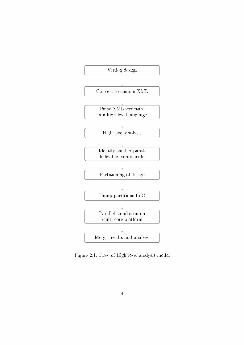
Figure 2.1: Flow of High level analysis model
4
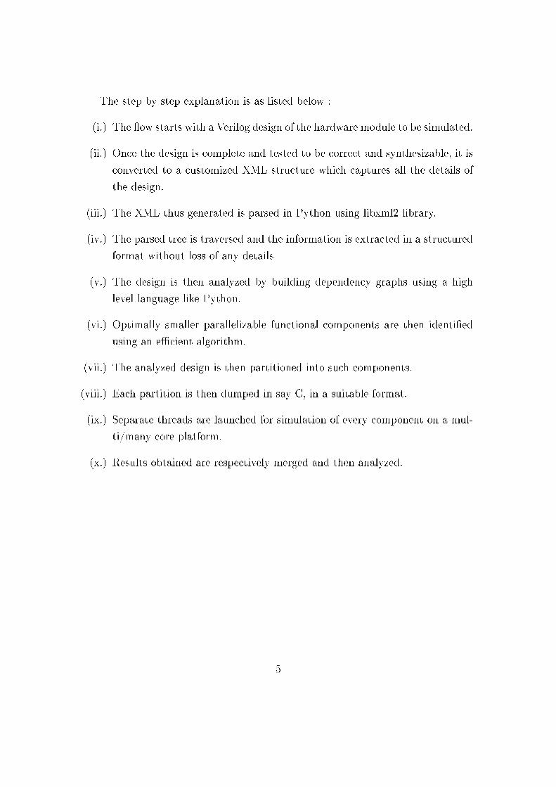
The step by step explanation is as listed below :
(i.) The �ow starts with a Verilog design of the hardware module to be simulated.
(ii.) Once the design is complete and tested to be correct and synthesizable, it is
converted to a customized XML structure which captures all the details of
the design.
(iii.) The XML thus generated is parsed in Python using libxml2 library.
(iv.) The parsed tree is traversed and the information is extracted in a structured
format without loss of any details
(v.) The design is then analyzed by building dependency graphs using a high
level language like Python.
(vi.) Optimally smaller parallelizable functional components are then identi�ed
using an e�cient algorithm.
(vii.) The analyzed design is then partitioned into such components.
(viii.) Each partition is then dumped in say C, in a suitable format.
(ix.) Separate threads are launched for simulation of every component on a mul-
ti/many core platform.
(x.) Results obtained are respectively merged and then analyzed.
5
Chapter 3
Verilog HDL's constructs supported
The project primarily focuses on the structural synthesisable hardware components
and the operations corresponding to them. As a result, only simple but essential
to hardware features are supported by this tool and it serves our purpose. Many
components of the HDLs like Verilog, which are often used by designers, but are
not implemented at hardware level are not considered in this project. Neverthe-
less, some features like initial blocks and memories are supported, but not much
emphasis is really upon them.
The comprehensive list of all the features supported is as follows:
3.1 wires and regs
Both wires and registers/�ip-�ops are supported by the tool. It stores all the
information associated with them like type, number of bits etc. and supports all
the operations possible upon them. Also, vectors of such wires/regs is also fully
supported. The various types of assignment operations possible are supported as
follows:
� assign statements
Continuous assignment upon wires as by assign statements outside sequen-
tial blocks, in Verilog.
6
� blocking and non-blocking assignments Sequential assignments to regs
by blocking/non-blocking assignment statements.
3.2 Independent hardware blocks
Hardware blocks acting in unison but independently and parallely, inside any hard-
ware module, like always blocks in Verilog are fully supported, with each individual
block having its own information such as its sensitivity lists, and the list of all the
sequential/combinational statements contained inside, in a structured manner.
3.3 Decision structures (MUXs)
Structures like MUXs which responsible for taking the decisions, depending upon
the current state of the hardware module and other control signals, are supported
in form of two Verilog constructs -
� case statements
case statements, with one control parameter to be compared across several
alternatives and accordingly decision taken, about which sequential block to
run at a particular state.
� if-else statements
if-else construct in which particular sequential hardware blocks are exe-
cuted depending upon the truth value of a Boolean conditional expression.
3.4 Additional support features
As described above, some constructs which are not very important from synthesis
point of view, but are still supported by this tool are as follows:
� initial blocks
Blocks assigning starting or 'initial' values to the regs, which is not synthe-
sisable but nevertheless important from the simulation perspective.
7
� Memories
Memories can be perceived as arrays of bit-vectors, with properly de�ned
range in both dimensions. These are also supported by this tool, although
their use from synthesis perspective is discouraged.
3.5 Ambiguity resolving features
There are some constructs in Verilog, which do not directly do what is apparent
on the face of it. They have to be carefully analyzed and their consequences,
accordingly evaluated. Two of these cases have been handled by the tool. They
are:
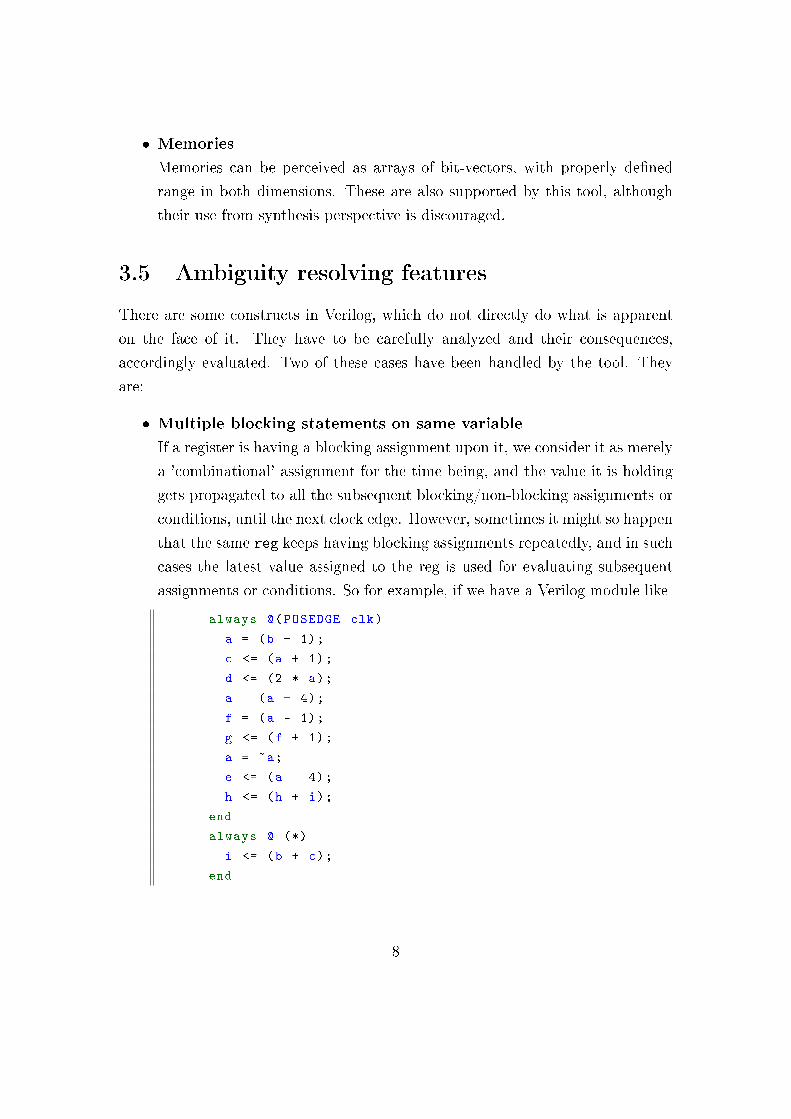
� Multiple blocking statements on same variable
If a register is having a blocking assignment upon it, we consider it as merely
a 'combinational' assignment for the time being, and the value it is holding
gets propagated to all the subsequent blocking/non-blocking assignments or
conditions, until the next clock edge. However, sometimes it might so happen
that the same reg keeps having blocking assignments repeatedly, and in such
cases the latest value assigned to the reg is used for evaluating subsequent
assignments or conditions. So for example, if we have a Verilog module like
always @(POSEDGE clk)
a = (b + 1);
c <= (a + 1);
d <= (2 * a);
a = (a + 4);
f = (a - 1);
g <= (f + 1);
a = ~a;
e <= (a - 4);
h <= (h + i);
end
always @ (*)
i <= (b + c);
end
8
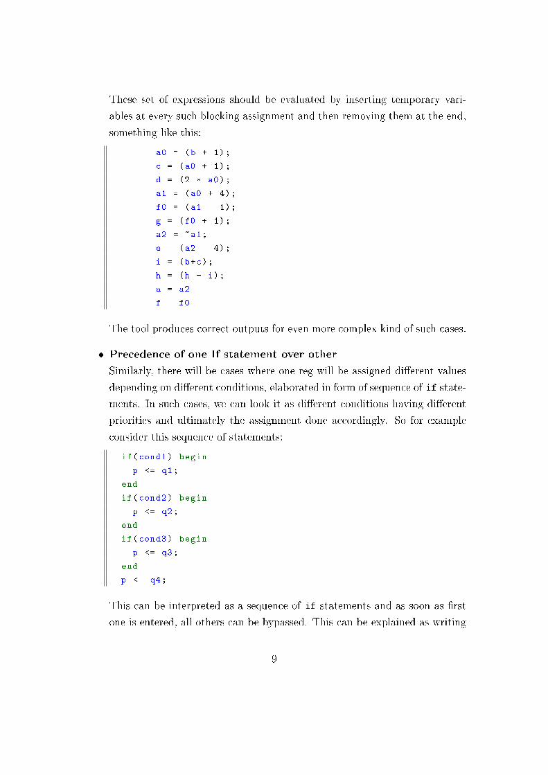
These set of expressions should be evaluated by inserting temporary vari-
ables at every such blocking assignment and then removing them at the end,
something like this:
a0 = (b + 1);
c = (a0 + 1);
d = (2 * a0);
a1 = (a0 + 4);
f0 = (a1 - 1);
g = (f0 + 1);
a2 = ~a1;
e = (a2 - 4);
i = (b+c);
h = (h + i);
a = a2
f = f0
The tool produces correct outputs for even more complex kind of such cases.
� Precedence of one If statement over other
Similarly, there will be cases where one reg will be assigned di�erent values
depending on di�erent conditions, elaborated in form of sequence of if state-
ments. In such cases, we can look it as di�erent conditions having di�erent
priorities and ultimately the assignment done accordingly. So for example
consider this sequence of statements:
if(cond1) begin
p <= q1;
end
if(cond2) begin
p <= q2;
end
if(cond3) begin
p <= q3;
end
p <= q4;
This can be interpreted as a sequence of if statements and as soon as �rst
one is entered, all others can be bypassed. This can be explained as writing
9
the priorities to assign p from bottom up, i.e., priority wise
(i.) Highest priority is of q4, and that too unconditionally
(ii.) q3 is of 2nd highest priority depending on cond3
(iii.) q2 is of 3rd highest priority depending on cond2 AND (NOT cond3)
(iv.) q1 is of least priority depending on cond1 AND (NOT cond2) AND (NOT
cond1)
As discussed above, all the essential structural hardware features are fully
supported by the tool and can be applied as such.
10
Chapter 4
Structure of the high level model
In this chapter the basic structure of the Python data structure used to store
the information of the hardware module is explained. The whole module is
stored as mainModule object which belongs to Module class. It consists of
three main parts, viz., ports, declarations and statements.
4.1 ports
A list of all the input and output ports of the top module is maintained
in form of a Python list. Every port holds information about the name,
direction (input/output), range (in case of bit-vectors) etc.
4.2 declarations
All the regs, wires and memories including the input and output ports, have
to be declared subsequent to module signature. All that information is stored
in form of three lists. Each member of the �rst two lists, hold all the informa-
tion about name, scalar type, range and endianness (in case of bit vectors)
etc. The list of memories, apart from these things also stores the details of
memory range and word range.
11
4.2.1 list of registers
Each member of the list, holds the information about name, scalar type,
range and endianness (in case of bit vectors) etc.
4.2.2 list of wires
Same as that of reg, each member holding the information about name, scalar
type, range and endianness (in case of vectors) etc.
4.2.3 list of memories
The list of memories, along with the above things, also stores the details of
memory range and word range.
4.3 statements
The third section contains all the continuous and sequential statements and
captures everything about the functionality of the hardware. It is subdivided
into three parts.
4.3.1 assign statements
All the continuous assignment statements are stored in a list of objects of a
dedicated class and hence captures all the the information about the assigned
value and their assignee.
4.3.2 initial block
The initial block too has a dedicated class, although it contains nothing
but an object of the statement block class, which captures all the statements
inside the initial block in form of statements' list.
12
4.3.3 always blocks
All the always blocks are then traversed through, and are appended to the
list of objects of always blocks class, where each always block object contains
essentially of two parts, a sensitivity list containing all the signals to whom
the block is sensitive to; and a list of statements object, which captures all
the sequential assignment inside the block.
13
Chapter 5
Details of implementation
This chapter goes into the ground level implementation of the various classes
and functions used for the di�erent features incorporated in the tool. Dif-
ferent constructs which it supports and the basic structure of the high level
model has already been talked about in the previous chapter. In this chap-
ter, we go one level deeper and understand the details of the structure and
the method used to implement.
5.1 Classes used
The model used is quite object oriented, with separate individual classes for
every independent structure and sub-structure. every class de�ned has its
member functions to store the value speci�c to the hardware construct it is
supporting. Following are the classes that have been de�ned and used.
5.1.1 Class mainModule
The top class which, corresponds to the main Verilog module is, named
mainModule. Its kept as simple as possible, by classifying it in three major
categories- ports, declarations and statements. Its structure, as a result is
quite straightforward.
14
mainModule:
list_of_ports
list_of_declarations
list_of_statements
As the names are quite self-explanatory, the three data members hold the
information about all the ports, declarations and statements, in the form of
Python lists of respective objects.
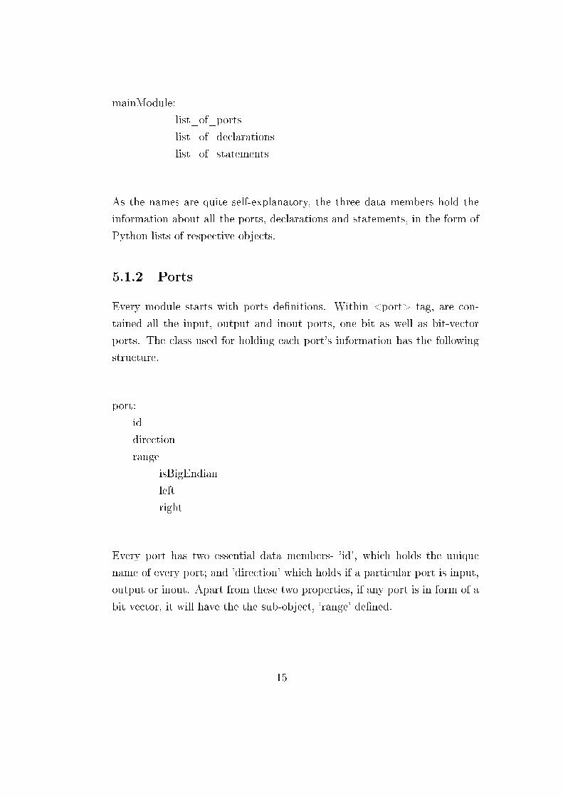
5.1.2 Ports
Every module starts with ports de�nitions. Within <port> tag, are con-
tained all the input, output and inout ports, one bit as well as bit-vector
ports. The class used for holding each port's information has the following
structure.
port:
id
direction
range
isBigEndian
left
right
Every port has two essential data members- 'id', which holds the unique
name of every port; and 'direction' which holds if a particular port is input,
output or inout. Apart from these two properties, if any port is in form of a
bit vector, it will have the the sub-object, 'range' de�ned.
15
5.1.2.1 Range class
Range class, which will also be used in subsequent class de�nitions, further
contains 3 information.
i. isBigEndian - range is to be read as big-endian or little-endian
ii. left - the left limit of range; and
iii. right- the right limit of range
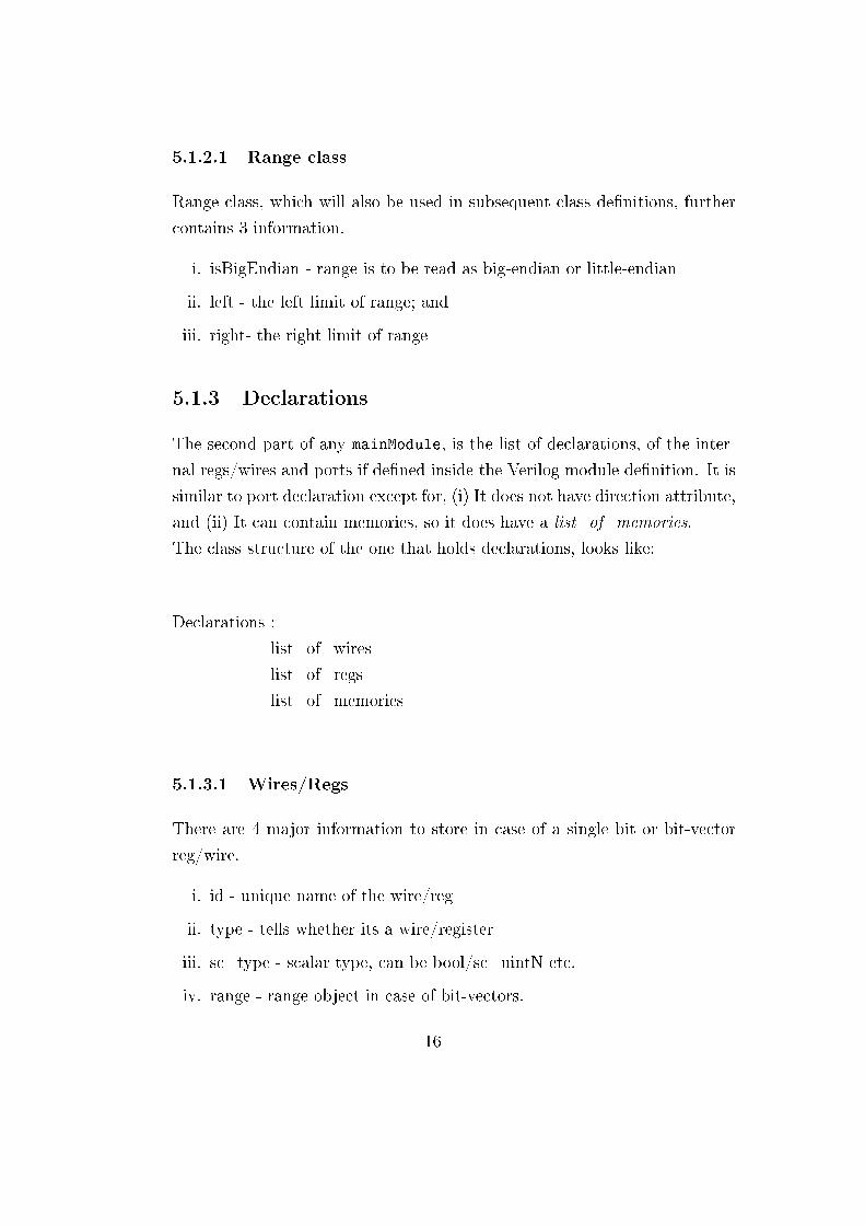
5.1.3 Declarations
The second part of any mainModule, is the list of declarations, of the inter-
nal regs/wires and ports if de�ned inside the Verilog module de�nition. It is
similar to port declaration except for, (i) It does not have direction attribute,
and (ii) It can contain memories, so it does have a list_of_memories.
The class structure of the one that holds declarations, looks like:
Declarations :
list_of_wires
list_of_regs
list_of_memories
5.1.3.1 Wires/Regs
There are 4 major information to store in case of a single bit or bit-vector
reg/wire.
i. id - unique name of the wire/reg
ii. type - tells whether its a wire/register
iii. sc_type - scalar type, can be bool/sc_uintN etc.
iv. range - range object in case of bit-vectors.
16
Note that any declaration can be characterized just by the id, type (wire or
reg) and sc_type information (uniquely telling about if its just a single bit
reg/wire or an N-bit wire/reg bit-vector). The range object, as described
earlier, stores information on endianness, left and right limits, in case of a
bit-vector.
5.1.3.2 Memories
Since most of the things in a memory is �xed (e.g. type always being reg),
memory has only 3 information that need to be stored- S
i. id - unique name of the memory
ii. mem_range - length of the bit-vector array (range object)
iii. word_range - length of each word of memory (range object)
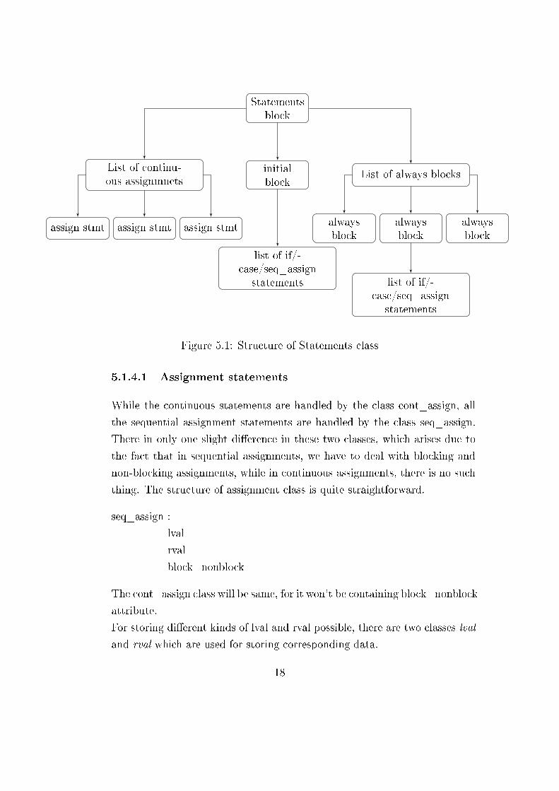
5.1.4 Statements
After the ports and declarations in a module are captured, there comes
the portion to capture the statements. This section e�ectively contains all
the functionalities of any module. This can be divided to three portions-
continuous assignments, initial block and always blocks. The method to
capture the functionality has to generic to maintain hierarchy. The structure
is explained by the �owchart in Figure 5.1
� First part is a list holding multiple objects of continuous assignment
type
� Second part contains a single InitialBlock object, which in turn con-
tains, a statement_list of various types, namely if, case or sequential
assignment.
� Third part is again a list, holding multiple always block objects. Each
always block object contains two lists, a sensitivity_list and a state-
ment_list.
17
Statementsblock
List of continu-ous assignmnets
initialblock
List of always blocks
assign stmt assign stmt assign stmt alwaysblock
alwaysblock
alwaysblock
list of if/-case/seq_assign
statements list of if/-case/seq_assign
statements
Figure 5.1: Structure of Statements class
5.1.4.1 Assignment statements
While the continuous statements are handled by the class cont_assign, all
the sequential assignment statements are handled by the class seq_assign.
There in only one slight di�erence in these two classes, which arises due to
the fact that in sequential assignments, we have to deal with blocking and
non-blocking assignments, while in continuous assignments, there is no such
thing. The structure of assignment class is quite straightforward.
seq_assign :
lval
rval
block_nonblock
The cont_assign class will be same, for it won't be containing block_nonblock
attribute.
For storing di�erent kinds of lval and rval possible, there are two classes lval
and rval which are used for storing corresponding data.
18
Class lval: The token on the left hand side of assignment operator, or the
token to which the value is being assigned is called lvalue. Here we have
named it as lval. There are multiple applications of assignment operation
according to which there are di�erent types of lvals possible. Some them to
count are:
(i.) simple −→ eg a <= 2′b10;
(ii.) bit-select −→ eg a[2] <= 1′b1;
(iii.) part-select −→ eg a[1 : 2] <= 2′b01;
(iv.) concatenated −→ eg {a, b} <= 4′b1011;1
As a result the class required to hold this kind of versatile data should take
care of this. The class used here has following attributes:
i. name : The unique id of the variable of lvalue
ii. type : Tells which type of lval it is, simple, bit-select or part-select
iii. index : for bit-select case, this tells the index
iv. isBigEndian : for part-select case, this tells the endianness of the range
v. left : for part-select case, this tells the left limit of the range
vi. right : for part-select case, this tells the right limit of the range
Class rval: Similarly, the token on the right hand side of assignment op-
erator, or the token whose value is being assigned to lvalue is called rvalue.
Here we have named it as rval. There are di�erent types of rvals possible.
Some them to count are:
(i.) simple −→ eg a <= 2′b10;
(ii.) binary operation −→ eg a <= b+ c;
(iii.) n-ary operation −→ eg a <= b+ c+ d+ e;
(iv.) concatenated −→ eg a <= {b, c};1This tool is yet to support concatenation type of lval. It'll be supported soon.
19
(v.) N-concatenated −→ eg a <= N{b};2
The class constructed to rval has the following structure:
rval:
name
binary_op
lvalue
rvalue
binop
The structure can be explained as follows:
i. name : In case of simple rval, it is the id of the variable on RHS
ii. binary_op : In case of binary operation, rval contains its object, which
contains-
(a) lvalue : The operand on left side of the binary operator
(b) rvalue : The operand on right side of the binary operator
(c) binop : The binary operator joining lvalue and rvalue
In case of n-ary operations, the XML is constructed such that, it looks like
a nested binary operation. Hence it can easily be parsed by recursively cre-
ating objects of class binary_op. So for example:
a <= b+ c+ d+ e;
can be considered as
a <= b+ (c+ (d+ e))
or may be
a <= (b+ c) + (d+ e)
2This tool is yet to support concatenation and N-concatenation types of rval.
20
5.1.4.2 If-Else statement
The second type of statements supported are if_else blocks. This block has
a dedicated class, essentially composed of three components:
(i.) cond_expr : Typically being a binary_op, it holds the conditional ex-
pression upon which if statement depends
(ii.) if_block : list of statements, contained in if part.
(iii.) else_block : list of statements, contained in else part.
5.1.4.3 Case statement
The structure of the class used to hold case statements is:
case_stmt:
select
case_item_list
case_item
alternative
statement_list
The explanation to the structure is as follows :
(i.) select : The lval on which case is de�ned, i.e., which has to be compared
(ii.) case_item_list : The list of object case_item which is described below
(iii.) case_item : Each case_item is individually capable of holding one case.
It contains two components-
a.) alt : The potential alternative value for select variable to hold
b.) stmt_list : The list of statements corresponding to each alternative
21
Chapter 6
Validation of the parsed results
To verify the correctness of the results obtained by the tool, another Python
�le was prepared, which takes as input the mainModule object (the topmost
object containing all the information about the hardware design module
hierarchically) and prints to console, the Verilog syntactic representation
of the information the mainModule object is holding. This 'pretty-printed'
generated Verilog is compared with the original Verilog design �le from which
the xml was generated initially. No loss of information is found in the new
�le, upon comparison. Thus the correctness of the script is veri�ed.
The �le doing this task, emitFunctions.py, contains a class Emitter which
reads the mainModule upon construction and using its methods:
(i.) emitDeclarations(): includes declarations for input/output ports and
intermediate regs/wires and memories.
(ii.) emitStatement(): covers all continuous assign statements.
(iii.) emitInitBlock(): dumps the initial block, and all its statements, if
present in the original design.
(iv.) emitAlwaysBlock(): includes all the always blocks present, with their
sensitivity list, and all the sequential statements contained in them
hierarchically.
A snapshot of sample emitted out Verilog code is shown in Figure A.2 Also,
22
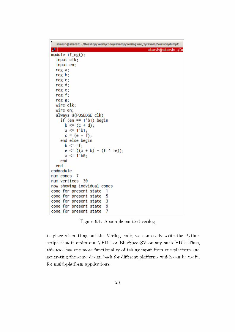
Figure 6.1: A sample emitted verilog
in place of emitting out the Verilog code, we can easily write the Python
script that it emits out VHDL or BlueSpec SV or any such HDL. Thus,
this tool has one more functionality of taking input from one platform and
generating the same design back for di�erent platforms which can be useful
for multi-platform applications.
23
Chapter 7
Analysis of parsed Verilog design
After the xml converted verilog design is parsed and veri�ed to be correct,
we need to put it to productive use. For this purpose, the single clock verilog
design was decided to be represented in form of a graph, capturing each and
every dependency of all the �ip �ops within two consecutive clock cycles, and
combinationally driven wires and regs. In this graph, the nodes can be �ip-
�ops, combinational regs, wires, unary/binary operators, 2-MUXs (If-else
statements), Priority Ifs (for multiple-if-driven Flip-Flops) and constants.
The edges capture the dependency between di�erent nodes, or basically de-
pendency of Flip-�op's present state on some or all �ip-�ops' previous state
and constants. The nodes and edges are colour coded categorically for easy
understanding of the user.
7.1 Construction of graph
The �le graphClass.py contains the de�nition of the class ModuleGraph,
an instance of which is constructed with mainModule object as the argu-
ment. It reads through the its structure, holding all the information about
Verilog design and systematically constructs graph, adding/removing nodes
and capturing dependencies, and adding edges �nally. The meanings for
24
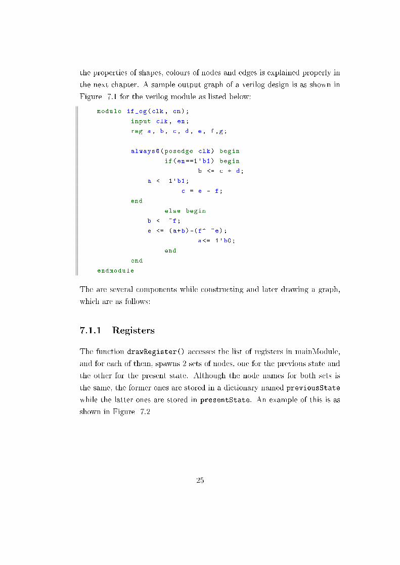
the properties of shapes, colours of nodes and edges is explained properly in
the next chapter. A sample output graph of a verilog design is as shown in
Figure 7.1 for the verilog module as listed below:
module if_eg(clk , en);
input clk , en;
reg a, b, c, d, e, f,g;
always@(posedge clk) begin
if(en==1'b1) begin
b <= c + d;
a <= 1'b1;
c = e - f;
end
else begin
b <= ~f;
e <= (a+b)-(f^ ~e);
a<= 1'b0;
end
end
endmodule
The are several components while constructing and later drawing a graph,
which are as follows:
7.1.1 Registers
The function drawRegister() accesses the list of registers in mainModule,
and for each of them, spawns 2 sets of nodes, one for the previous state and
the other for the present state. Although the node names for both sets is
the same, the former ones are stored in a dictionary named previousState
while the latter ones are stored in presentState. An example of this is as
shown in Figure 7.2
25
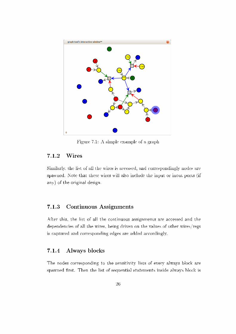
Figure 7.1: A simple example of a graph
7.1.2 Wires
Similarly, the list of all the wires is accessed, and correspondingly nodes are
spawned. Note that these wires will also include the input or inout ports (if
any) of the original design.
7.1.3 Continuous Assignments
After this, the list of all the continuous assignments are accessed and the
dependencies of all the wires, being driven on the values of other wires/regs
is captured and corresponding edges are added accordingly.
7.1.4 Always blocks
The nodes corresponding to the sensitivity lists of every always block are
spawned �rst. Then the list of sequential statements inside always block is
26
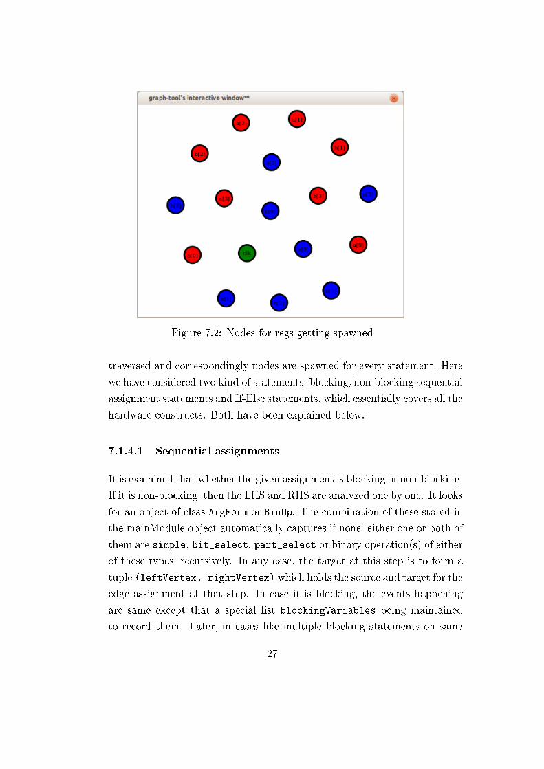
Figure 7.2: Nodes for regs getting spawned
traversed and correspondingly nodes are spawned for every statement. Here
we have considered two kind of statements, blocking/non-blocking sequential
assignment statements and If-Else statements, which essentially covers all the
hardware constructs. Both have been explained below.
7.1.4.1 Sequential assignments
It is examined that whether the given assignment is blocking or non-blocking.
If it is non-blocking, then the LHS and RHS are analyzed one by one. It looks
for an object of class ArgForm or BinOp. The combination of these stored in
the mainModule object automatically captures if none, either one or both of
them are simple, bit_select, part_select or binary operation(s) of either
of these types, recursively. In any case, the target at this step is to form a
tuple (leftVertex, rightVertex) which holds the source and target for the
edge assignment at that step. In case it is blocking, the events happening
are same except that a special list blockingVariables being maintained
to record them. Later, in cases like multiple blocking statements on same
27
variable, they are examined to remove the redundant nodes.
7.1.4.2 If-Else statements
Similar is the analysis here, searching for ArgForms and and returning vertex
pairs. Except that it is done thrice, one for the conditional expression, one for
the True scope and one for the False scope. Edges accordingly are di�erent.
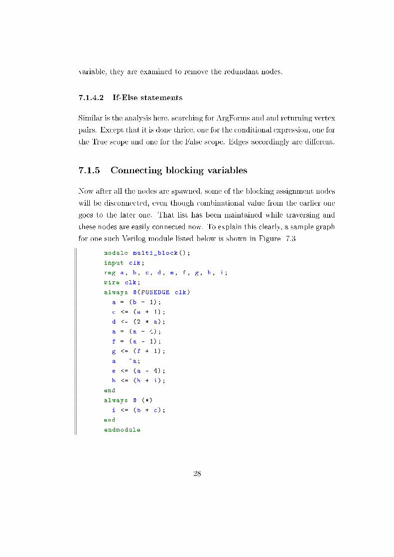
7.1.5 Connecting blocking variables
Now after all the nodes are spawned, some of the blocking assignment nodes
will be disconnected, even though combinational value from the earlier one
goes to the later one. That list has been maintained while traversing and
these nodes are easily connected now. To explain this clearly, a sample graph
for one such Verilog module listed below is shown in Figure 7.3
module multi_block ();
input clk;
reg a, b, c, d, e, f, g, h, i;
wire clk;
always @(POSEDGE clk)
a = (b + 1);
c <= (a + 1);
d <= (2 * a);
a = (a + 4);
f = (a - 1);
g <= (f + 1);
a = ~a;
e <= (a - 4);
h <= (h + i);
end
always @ (*)
i <= (b + c);
end
endmodule
28
These set of expressions should be evaluated by inserting temporary vari-
ables at every such blocking assignment and then removing them at the end,
something like this:
a0 = (b + 1);
c = (a0 + 1);
d = (2 * a0);
a1 = (a0 + 4);
f0 = (a1 - 1);
g = (f0 + 1);
a2 = ~a1;
e = (a2 - 4);
i = (b+c);
h = (h + i);
a = a2;
f = f0;
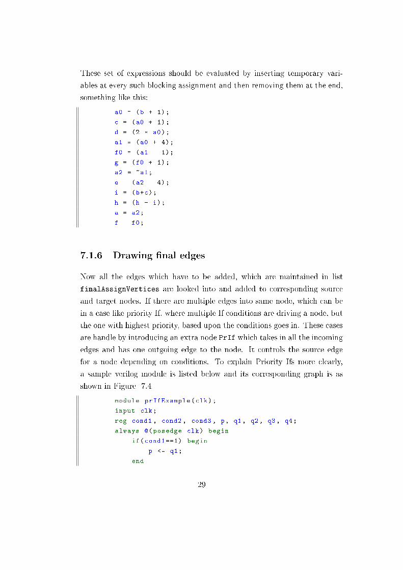
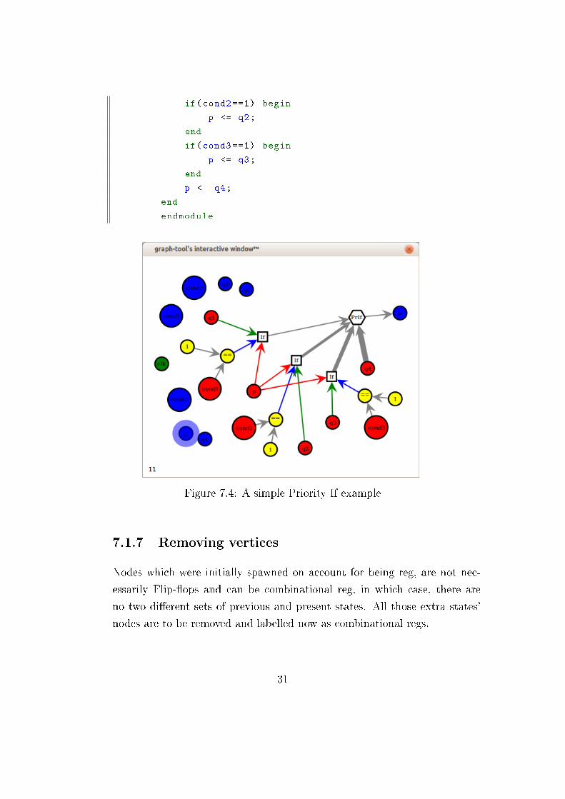
7.1.6 Drawing �nal edges
Now all the edges which have to be added, which are maintained in list
finalAssignVertices are looked into and added to corresponding source
and target nodes. If there are multiple edges into same node, which can be
in a case like priority If, where multiple If conditions are driving a node, but
the one with highest priority, based upon the conditions goes in. These cases
are handle by introducing an extra node PrIf which takes in all the incoming
edges and has one outgoing edge to the node. It controls the source edge
for a node depending on conditions. To explain Priority Ifs more clearly,
a sample verilog module is listed below and its corresponding graph is as
shown in Figure 7.4
module prIfExample(clk);
input clk;
reg cond1 , cond2 , cond3 , p, q1 , q2 , q3 , q4;
always @(posedge clk) begin
if(cond1 ==1) begin
p <= q1;
end
29
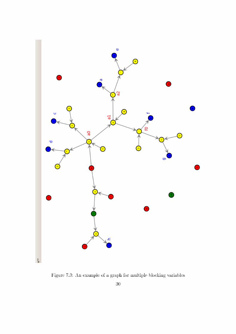
Figure 7.3: An example of a graph for multiple blocking variables
30
if(cond2 ==1) begin
p <= q2;
end
if(cond3 ==1) begin
p <= q3;
end
p <= q4;
end
endmodule
Figure 7.4: A simple Priority If example
7.1.7 Removing vertices
Nodes which were initially spawned on account for being reg, are not nec-
essarily Flip-�ops and can be combinational reg, in which case, there are
no two di�erent sets of previous and present states. All those extra states'
nodes are to be removed and labelled now as combinational regs.
31
Chapter 8
Extraction of Cones
A cone or logic cone is formally de�ned as a set of elements encountered
during a backtrace from an internal circuit node and to input state points. In
our application, the set of nodes and edges from a present state, backtracing
until a previous state or constant or input port is encountered, is what we
have called a cone of that particular present state.
For extraction of cones a class is de�ned in the �le graphClass.py, named
ConeGraph. For construction, it takes in an object of ModuleGraph class,
a set of vertex, a set of edges, and the present state for which the cone is
being constructed. The vertexset and edgeset, of course are generated in the
ModuleGraph itself inside the function findVariableCone() which iterates
back node by node backtracing till it �nds the terminal points, and returns
vertexSet and coneSet for that present state.
A sample cone for the variable 'a' of Figure 7.1 is as shown in the Figure 8.1
Similarly, for multiple blocking cases, the cones come out to be as expected.
An example cone for the variable 'g' of Figure 7.3 is shown in Figure 8.2
32
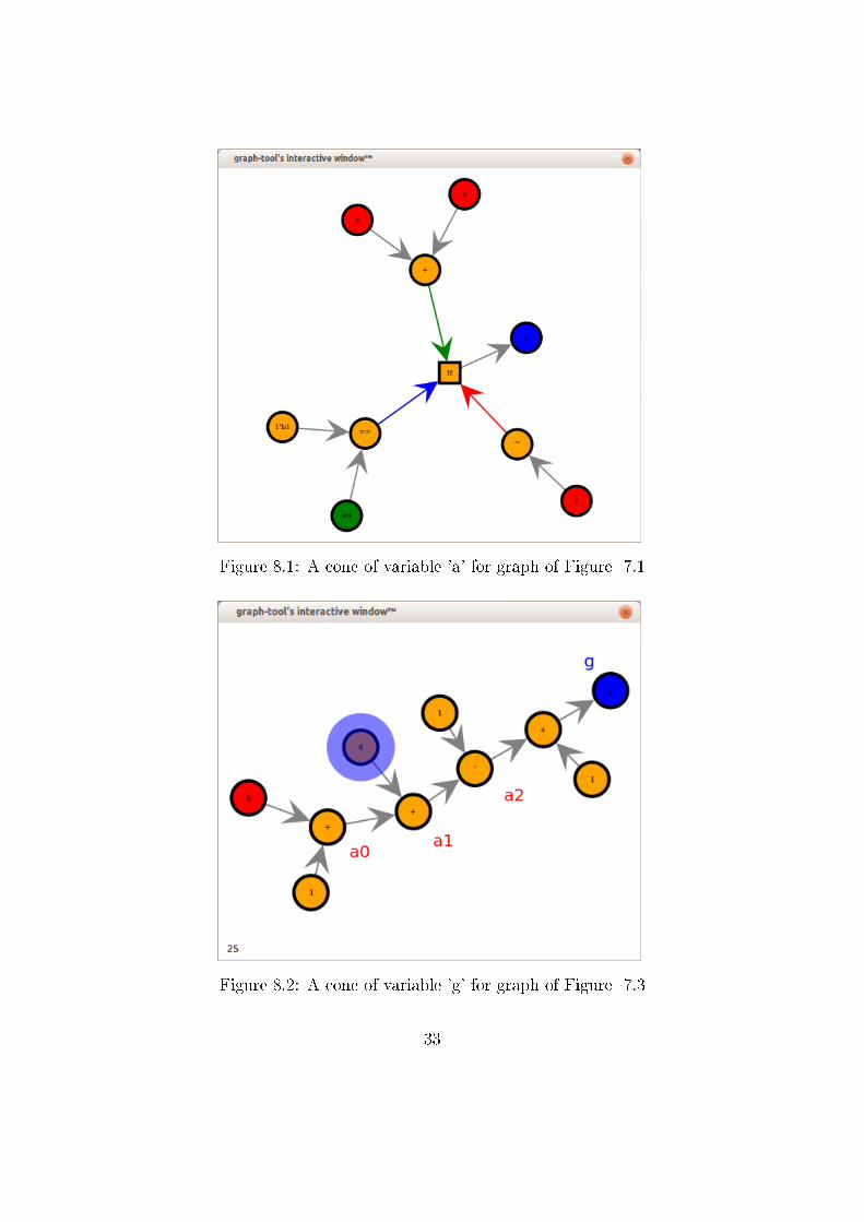
Figure 8.1: A cone of variable 'a' for graph of Figure 7.1
Figure 8.2: A cone of variable 'g' for graph of Figure 7.3
33
Chapter 9
Visualization of the graphs
constructed
The graphs now constructed fully are holding each and every information
happening between two consecutive clock edges, in a single clock verilog de-
sign. They are dumped in standard graphml format, to be read and analyzed
again by other programs or scripts. In fact, we will see in coming chapters,
where these graphs are analyzed for inter-dependency and their independent
and hence parallelizable components and accordingly be partitioned. Also
Python graph_tool module used upto now for constructing and manipulat-
ing our graph, also produces visually illustrative versions of the graphs if
we de�ne such properties. For user's readability and clearer understanding,
these features were fully utilized in our implementation. Some of these useful
properties are explained in subsequent sections.
9.1 Digital design and other information stored
in graphs
Some of the useful properties, were dumped along with dumping the graph,
in .graphml format. These are listed below:
34
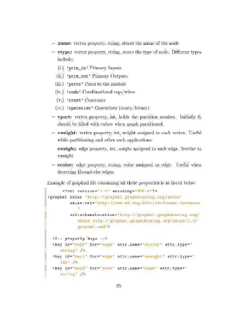
� name: vertex property, string, stores the name of the node
� vtype: vertex property, string, stores the type of node. Di�erent types
include:
(i.) 'prim_in' Primary Inputs
(ii.) 'prim_out' Primary Outputs
(iii.) 'ports' Ports to the module
(iv.) 'comb' Combinational regs/wires
(v.) 'const' Constants
(vi.) 'operation' Operations (unary/binary)
� vpart: vertex property, int, holds the partition number. Initially 0,
should be �lled with values when graph partitioned.
� vweight: vertex property, int, weight assigned to each vertex. Useful
while partitioning and other such applications.
� eweight: edge property, int, weight assigned to each edge. Similar to
vweight.
� ecolor: edge property, string, color assigned to edge. Useful when
detecting If-cond-else edges.
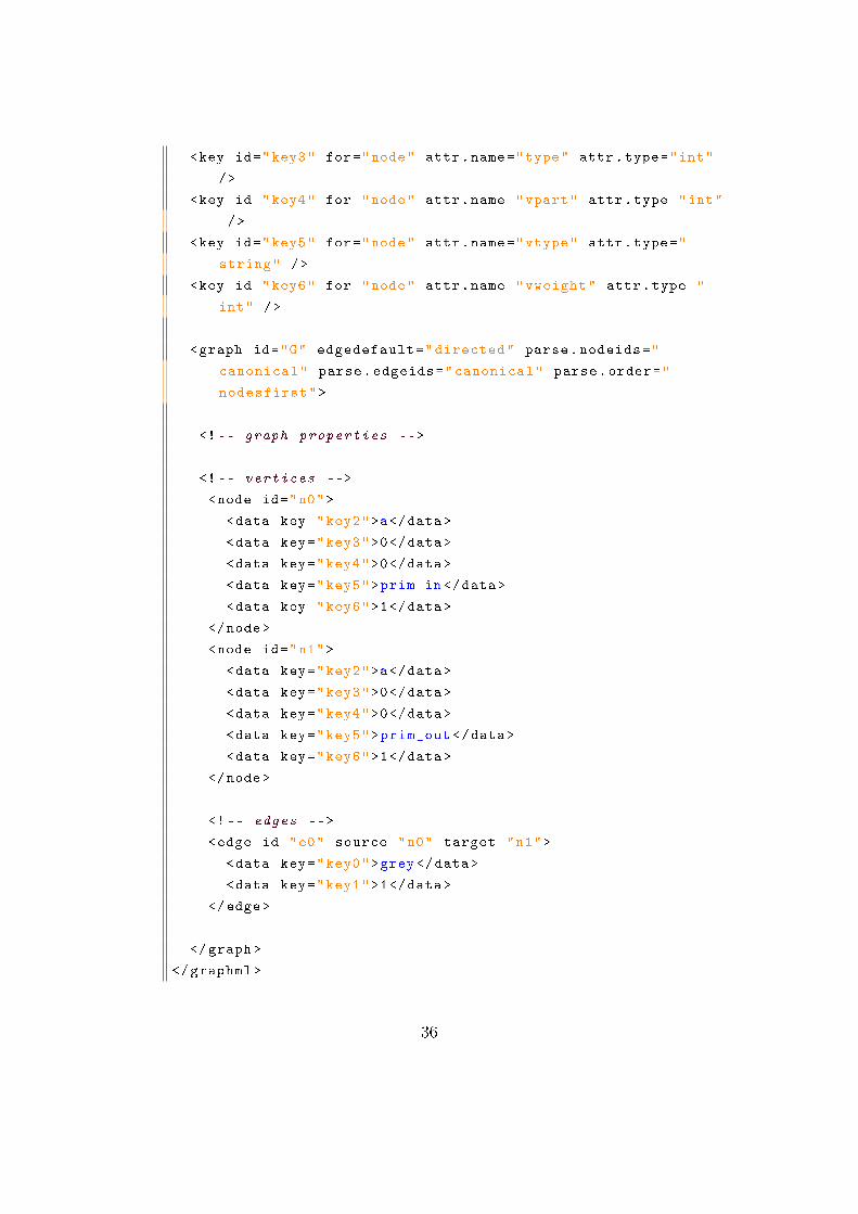
Example of graphml �le containing all these properties is as listed below
<?xml version="1.0" encoding="UTF -8"?>
<graphml xmlns="http: // graphml.graphdrawing.org/xmlns"
xmlns:xsi="http://www.w3.org /2001/ XMLSchema -instance
"
xsi:schemaLocation="http:// graphml.graphdrawing.org/
xmlns http: // graphml.graphdrawing.org/xmlns /1.0/
graphml.xsd">
<!-- property keys -->
<key id="key0" for="edge" attr.name="ecolor" attr.type="
string" />
<key id="key1" for="edge" attr.name="eweight" attr.type="
int" />
<key id="key2" for="node" attr.name="name" attr.type="
string" />
35
<key id="key3" for="node" attr.name="type" attr.type="int"
/>
<key id="key4" for="node" attr.name="vpart" attr.type="int"
/>
<key id="key5" for="node" attr.name="vtype" attr.type="
string" />
<key id="key6" for="node" attr.name="vweight" attr.type="
int" />
<graph id="G" edgedefault="directed" parse.nodeids="
canonical" parse.edgeids="canonical" parse.order="
nodesfirst">
<!-- graph properties -->
<!-- vertices -->
<node id="n0">
<data key="key2">a</data>
<data key="key3">0</data>
<data key="key4">0</data>
<data key="key5">prim_in </data>
<data key="key6">1</data>
</node>
<node id="n1">
<data key="key2">a</data>
<data key="key3">0</data>
<data key="key4">0</data>
<data key="key5">prim_out </data>
<data key="key6">1</data>
</node>
<!-- edges -->
<edge id="e0" source="n0" target="n1">
<data key="key0">grey</data>
<data key="key1">1</data>
</edge>
</graph>
</graphml >
36
9.2 Parent Graph visual scheme
The various colouring and shaping schemes used are as listed below:
1. Flip-�ops: Shape circle; Color, Red for previousState, Blue for pre-
sentState
2. Combinational regs/wires: Shape circle; Color Green
3. Operators: Shape Circle; Color Yellow
4. If statement:
� 'If' node: Shape Square, color White
� Condition Edge: Color Blue
� True Edge: Color Green
� False Edge: Color Red
5. Priority If: Shape Hexagon, Color White; more priority means thicker
edge.
6. Edges: All edges, except for special edges described above, Color Grey
9.3 Cone Graph visual scheme
Even in the cones' graphs:
� Present State �ip�ops still Blue; Previous state Flip�ops still Red
� Input Ports Green
� Rest all nodes Orange
� Special edges: 'If' CondEdges Blue, TrueEdges Green, FalseEdges Red,
Priority Edges accordingly thick
� All edges except special edges, Color Grey
37
Chapter 10
Conversion of cones to C threads
Once, we have the cones for all �ip-�ops, we can directly move to achieve
our goal of parallelizing hardware simulation by creating separate threads
for parallelizable components and simulate them, prior to merging and ana-
lyzing results. In our case we have, for the headstart, considered each cone
as one partition, which are de�nitely independent and easily parallelizable.
Of course, its not the most optimal solution, and there will be sub-cones
common to multiple cones which will be simulated more than once, which is
redundant. But for now, we have restricted ourselves to one cone simulated
on one core scheme, to look at the results.
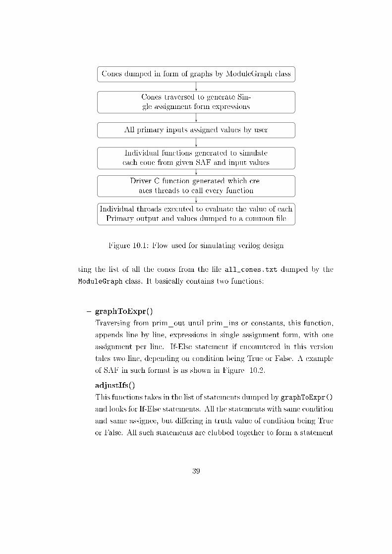
The step by step �ow used for simulating the whole verilog design is as shown
in the �owchart shown in Figure 10.1
These steps are explained in greater details in subsequent sections:
10.1 Cones to single assignment form expres-
sions
The cones for every �ip-�op in the verilog module, after being dumped in
.graphml format are read back in Python by the �le coneToSAF.py, by get-
38
Cones dumped in form of graphs by ModuleGraph class
Cones traversed to generate Sin-gle assignment form expressions
All primary inputs assigned values by user
Individual functions generated to simulateeach cone from given SAF and input values
Driver C function generated which cre-ates threads to call every function
Individual threads executed to evaluate the value of eachPrimary output and values dumped to a common �le
Figure 10.1: Flow used for simulating verilog design
ting the list of all the cones from the �le all_cones.txt dumped by the
ModuleGraph class. It basically contains two functions:
� graphToExpr()
Traversing from prim_out until prim_ins or constants, this function,
appends line by line, expressions in single assignment form, with one
assignment per line. If-Else statement if encountered in this version
tales two line, depending on condition being True or False. A example
of SAF in such format is as shown in Figure 10.2.
� adjustIfs()
This functions takes in the list of statements dumped by graphToExpr()
and looks for If-Else statements. All the statements with same condition
and same assignee, but di�ering in truth value of condition being True
or False. All such statements are clubbed together to form a statement
39
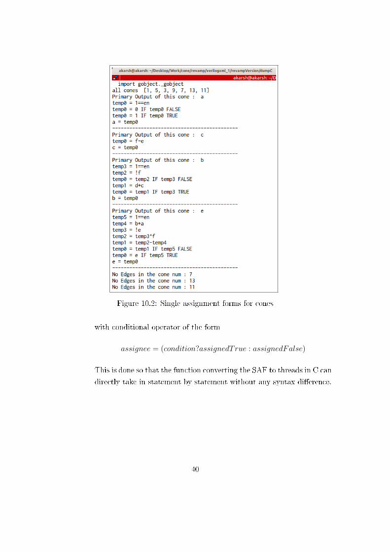
Figure 10.2: Single assignment forms for cones
with conditional operator of the form
assignee = (condition?assignedTrue : assignedFalse)
This is done so that the function converting the SAF to threads in C can
directly take in statement by statement without any syntax di�erence.
40
10.2 Assigning values to the inputs
The �le assignPrimIns.py looks at the dump�les from each cones and
makes a list of all possible primary inputs for all the cones, without any
input repeating, and dumps it in a �le all_inputs.txt, one variable per
line. The user is then expected to edit the �le all_inputs.txt and as-
sign each input a valid positive integer value in the format in the for-
mat variable <whitespace> = <whitespace> value; or alternatively
variable <whitespace> value. For example,
a = 1
en = 0
and so on.
OR
a 1
en 0
and so on.
10.3 SAFs to individual thread functions
10.3.1 Generating individual functions
Now, with the individual cones' SAFs present in dump �les and values of
all possible inputs present from user with us, we can now easily create func-
tions, which evaluate one cone each. These functions can then easily be
called with POSIX threads from the C code. All these functions are dumped
in a C header �le func_all_cones.h. Upon execution every function eval-
uates the value fo primary output of a cone and dumps it in the text �le
all_outputs.txt. A sample function is as shown below:
41
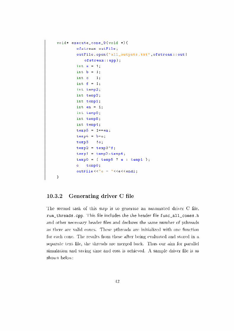
void* execute_cone_9(void *){
ofstream outFile;
outFile.open("all_outputs.txt",ofstream ::out|
ofstream ::app);
int a = 1;
int b = 1;
int e = 1;
int f = 1;
int temp3;
int temp2;
int temp1;
int en = 1;
int temp0;
int temp5;
int temp4;
temp5 = 1==en;
temp4 = b+a;
temp3 = !e;
temp2 = temp3^f;
temp1 = temp2 -temp4;
temp0 = ( temp5 ? e : temp1 );
e = temp0;
outFile <<"e = "<<e<<endl;
}
10.3.2 Generating driver C �le
The second task of this step is to generate an automated driver C �le,
run_threads.cpp. This �le includes the the header �le func_all_cones.h
and other necessary header �les and declares the same number of pthreads
as there are valid cones. These pthreads are initialized with one function
for each cone. The results from these after being evaluated and stored in a
separate text �le, the threads are merged back. Thus our aim for parallel
simulation and saving time and cost is achieved. A sample driver �le is as
shown below:
42
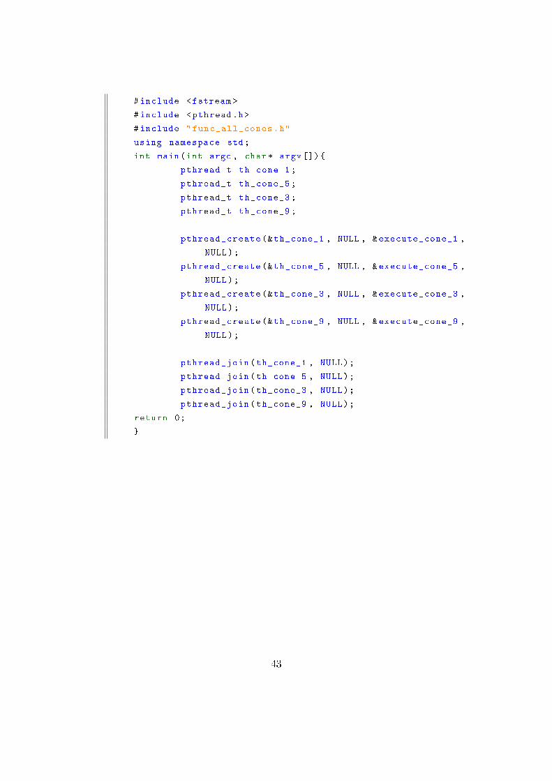
#include <fstream >
#include <pthread.h>
#include "func_all_cones.h"
using namespace std;
int main(int argc , char* argv []){
pthread_t th_cone_1;
pthread_t th_cone_5;
pthread_t th_cone_3;
pthread_t th_cone_9;
pthread_create (&th_cone_1 , NULL , &execute_cone_1 ,
NULL);
pthread_create (&th_cone_5 , NULL , &execute_cone_5 ,
NULL);
pthread_create (&th_cone_3 , NULL , &execute_cone_3 ,
NULL);
pthread_create (&th_cone_9 , NULL , &execute_cone_9 ,
NULL);
pthread_join(th_cone_1 , NULL);
pthread_join(th_cone_5 , NULL);
pthread_join(th_cone_3 , NULL);
pthread_join(th_cone_9 , NULL);
return 0;
}
43
Chapter 11
Toy Examples
The tool was used on several hardware modules. As explained earlier, the
�ow starts with designing the Verilog modules. The modules were then ver-
i�ed to be correct by writing their test benches and simulating them using
iverilog. After they are void of any errors and the output was as expected, the
XML �le is generated corresponding to the main module using the ToXML
tool created by my colleague, Dilawar Singh. The custom XML generated is
parsed and results are analyzed using the tool.
The Verilog designs are tried to be kept as simple but synthesizable as possi-
ble. Use of loops and memories is avoided as much as possible. The aim was
to demonstrate that the tool will work for designs that resemble to actual
circuit level hardware. The tool was tried on three Verilog designs which
are of slightly di�erent type. The �rst module considered is a behavioural
design of single cycle MIPS, second one is an elementary FSM based Matrix
multiplicator and the third one is a hardware module which determines if a
given element is present in memory, most e�ciently, implemented in form of
an FSM.
44
11.1 Single cycle mMIPS processor
A simpli�ed behavioural model of a single cycle mMIPS processor was im-
plemented in Verilog. It consisted of a clk, a reset, a 32 bit program counter
as registers and a 32-bit instruction is stored as a wire. It also contains 3
memories, a 32-element Register �le, and two 256-element Instruction and
Data memories, with word length throughout being 32-bits.
The simpli�ed model supports only some basic ones of the supported opera-
tions, just for the purpose of illustration. The list of the supported operations
are-
(i) add: addition of values in two registers
(ii) addi: addition of value in register and immediate data
(iii) sub: subtraction of values in two registers
(iv) beq: branch to a memory location if operands are equal
(v) load: load data from a memory location to register
(vi) store: store data to a memory location from register
(vii) jump: go to the given address unconditionally
The testbench was constructed to generate Fibonacci sequence, and the de-
sign delivers corrects results. So the top module being ready for analysis,
was converted to XML structure, and parsed using the tool and results were
obtained for analysis.
45
Cones dumped in form of graphs by ModuleGraph class
Cones traversed to generate Sin-gle assignment form expressions
All primary inputs assigned values by user
Individual functions generated to simulateeach cone from given SAF and input values
Driver C function generated which cre-ates threads to call every function
Individual threads executed to evaluate the value of eachPrimary output and values dumped to a common �le
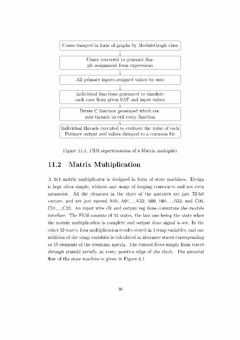
Figure 11.1: FSM representation of a Matrix multiplier
11.2 Matrix Multiplication
A 4x4 matrix multiplicator is designed in form of state machines. Design
is kept ultra simple, without any usage of looping constructs and not even
memories. All the elements in the three of the matrices are just 32-bit
vectors, and are just named A00, A01,...,A33; B00, B01,...,B33; and C00,
C01,...,C33. An input wire clk and output reg done constitute the module
interface. The FSM consists of 33 states, the last one being the state when
the matrix multiplication is complete and output done signal is set. In the
other 32 states, four multiplication results stored in 4 temp variables, and one
addition of the temp variables is calculated in alternate states corresponding
to 16 elements of the resultant matrix. The control �ows simply from state0
through state32 serially at every positive edge of the clock. The pictorial
�ow of the state machine is given in Figure 6.1
46
Simulation Results
Initial values of matrix A
A00 = 1; A01 = 2; A02 = 3; A03 = 4
A10 = 5; A11 = 6; A22 = 7; A23 = 8
A20 = 9; A21 = 10; A22 = 11; A23 = 12
A30 = 13; A31 = 14; A32 = 15; A33 = 16
Initial values of B00 - B33
B00 = 1; B01 = 1; B02 = 1; B03 = 1
B10 = 1; B11 = 1; B22 = 1; B23 = 1
B20 = 1; B21 = 1; B22 = 1; B23 = 1
B30 = 1; B31 = 1; B32 = 1; B33 = 1
Final values of C00 - C33
C00 = 10; C01 = 10; C02 = 10; C03 = 10
C10 = 20; C11 = 20; C22 = 20; C23 = 20
C20 = 30; C21 = 30; C22 = 30; C23 = 30
C30 = 40; C31 = 40; C32 = 40; C33 = 40
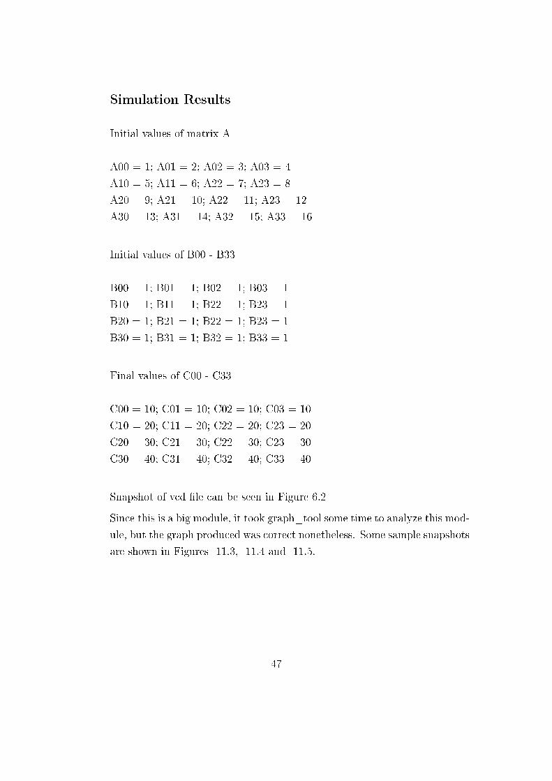
Snapshot of vcd �le can be seen in Figure 6.2
Since this is a big module, it took graph_tool some time to analyze this mod-
ule, but the graph produced was correct nonetheless. Some sample snapshots
are shown in Figures 11.3, 11.4 and 11.5.
47
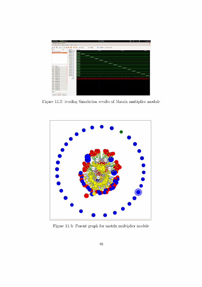
Figure 11.2: iverilog Simulation results of Matrix multiplier module
Figure 11.3: Parent graph for matrix multiplier module
48
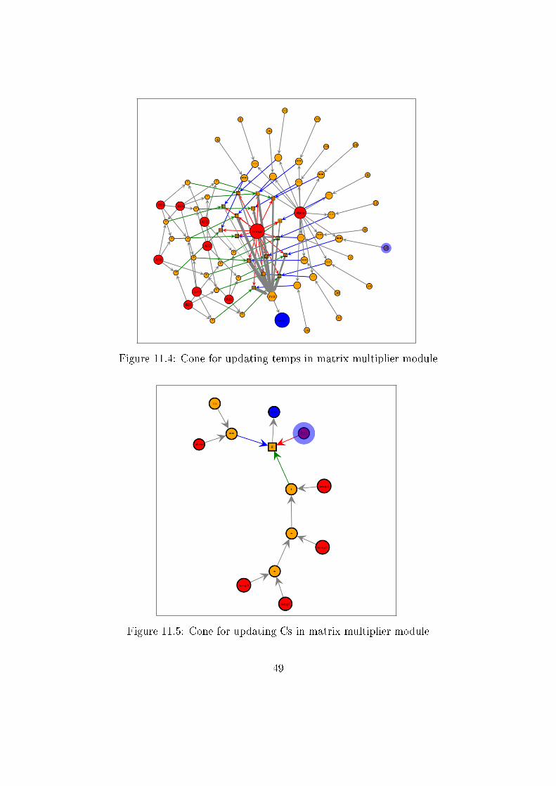
Figure 11.4: Cone for updating temps in matrix multiplier module
Figure 11.5: Cone for updating Cs in matrix multiplier module
49
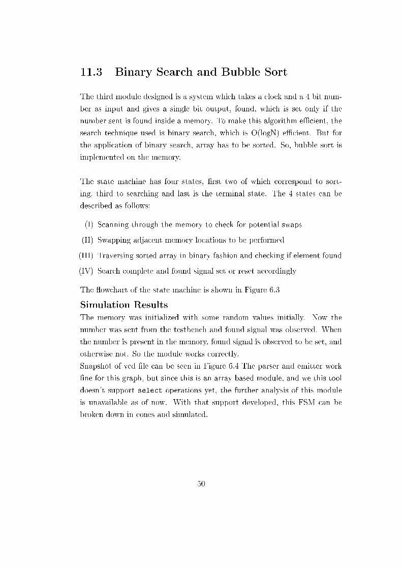
11.3 Binary Search and Bubble Sort
The third module designed is a system which takes a clock and a 4 bit num-
ber as input and gives a single bit output, found, which is set only if the
number sent is found inside a memory. To make this algorithm e�cient, the
search technique used is binary search, which is O(logN) e�cient. But for
the application of binary search, array has to be sorted. So, bubble sort is
implemented on the memory.
The state machine has four states, �rst two of which correspond to sort-
ing, third to searching and last is the terminal state. The 4 states can be
described as follows:
(I) Scanning through the memory to check for potential swaps
(II) Swapping adjacent memory locations to be performed
(III) Traversing sorted array in binary fashion and checking if element found
(IV) Search complete and found signal set or reset accordingly
The �owchart of the state machine is shown in Figure 6.3
Simulation ResultsThe memory was initialized with some random values initially. Now the
number was sent from the testbench and found signal was observed. When
the number is present in the memory, found signal is observed to be set, and
otherwise not. So the module works correctly.
Snapshot of vcd �le can be seen in Figure 6.4 The parser and emitter work
�ne for this graph, but since this is an array based module, and we this tool
doesn't support select operations yet, the further analysis of this module
is unavailable as of now. With that support developed, this FSM can be
broken down in cones and simulated.
50
State == 0?
State == 1
State == 2
State == 3
j == 8-1? Yes Yes j = 0
No No
No
Yes
Counter==0? Counter=0
arr[j]<arr[j+1]? Yes
No
arr[j]<=arr[j+1]; arr[j+1]<=arr[j];
Arr[mid]==
num?
Arr[mid]<
num?
first> last?
Yes
No
No
No
p
Yes
Yes
Yes Yes
Mid = (first+last)/2
First = mid+1 Mid = (first+last)/2
First = mid+1
found = 1
Yes
Arr[mid]>
num?
found = 0
NoNo
Figure 11.6: Pictorial representation of SearchSort FSM
51
Figure 11.7: iverilog Simulation results of SearchSort module
52
Chapter 12
Conclusions and Future Work
12.1 Results achieved
As evident by the results, we have successfully been able to parallelize the
hardware simulation in a very systematic manner. The Verilog converted to
standard XML structure, which is parsed in Python. The information cap-
tured in Python is then e�ciently used to de�ne dependencies, in accordance
with which individual threads are executed to simulate the whole design par-
allely, speeding up and automating the whole process. The benchmarking is
not yet done. Only correctness has been veri�ed. E�ciency aspects are to
be explored in future work in this project.
12.2 Further utilities
The intermediate resources developed during these are quite useful and can
easily be extended to other application. The VerilogToXML generator gen-
erates a custom structure standard format XML, which can easily be used by
di�erent applications, and upon di�erent platforms. The Emitter tool can
emit out the same data in di�erent HDLs like VHDL, Bluespec SV etc and
hence can come out to be quite useful fr such multi-platform applications.
The dependency graphs generated starting from a single-clock verilog design
53
are in .graphml format, which again can be used by other applications. par-
titioning of graphs for numerous other purposes can be thought of, which
can be bene�ted by these tools.
12.3 Suggested improvements and additions
Although, the results are fairly good, the project can in no way be said to
be complete. There are a lot of features which can be improved upon to
make the tool more e�cient. To name a few, construction of cone from a
graph, and generating SAF from cones can be made more e�cient. Moreover,
many features are not present, which can add up a lot to the utility to the
tool. So for example, Bit-wise operations, though parsed completely and
correctly, are still not supported for graph-build up and simulation. More
importantly, as of now now, the parallelisation is at very basic level, one
cone for one thread. There can be a lot of redundancy in that. Sub-cones
common to many cones are being simulated more than once unnecessarily.
With more e�cient partitioning techniques, this tool can prove to be a lot
more e�ective and useful.
54
Appendix A
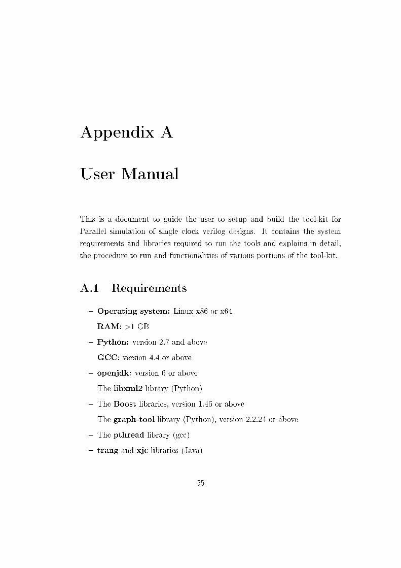
User Manual
This is a document to guide the user to setup and build the tool-kit for
Parallel simulation of single clock verilog designs. It contains the system
requirements and libraries required to run the tools and explains in detail,
the procedure to run and functionalities of various portions of the tool-kit.
A.1 Requirements
� Operating system: Linux x86 or x64
� RAM: >1 GB
� Python: version 2.7 and above
� GCC: version 4.4 or above
� openjdk: version 6 or above
� The libxml2 library (Python)
� The Boost libraries, version 1.46 or above
� The graph-tool library (Python), version 2.2.24 or above
� The pthread library (gcc)
� trang and xjc libraries (Java)
55
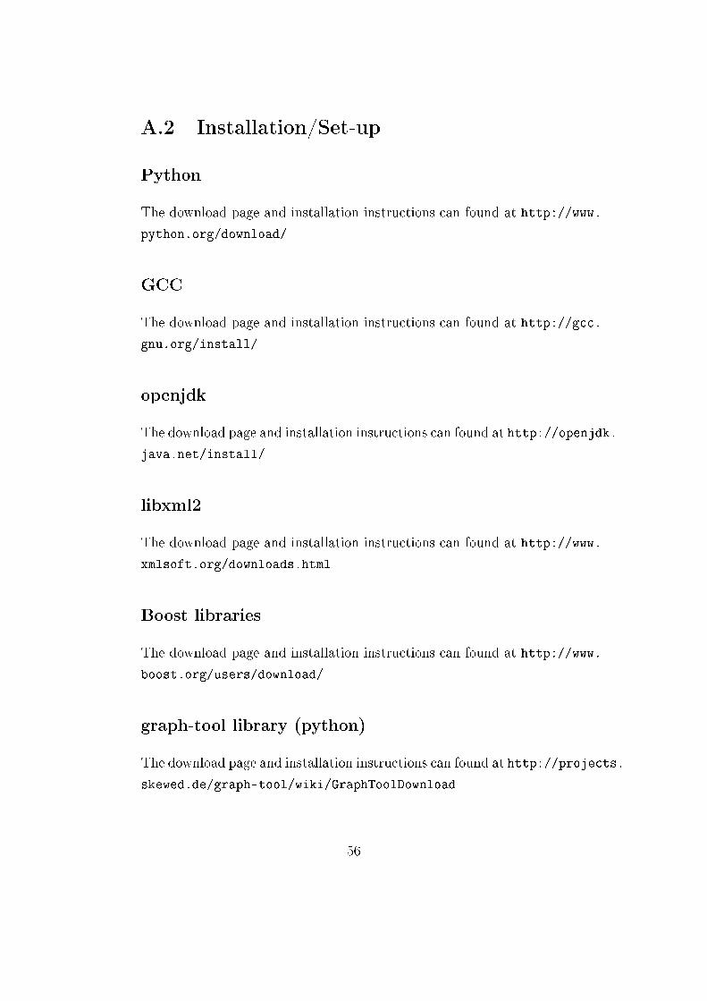
A.2 Installation/Set-up
Python
The download page and installation instructions can found at http://www.
python.org/download/
GCC
The download page and installation instructions can found at http://gcc.
gnu.org/install/
openjdk
The download page and installation instructions can found at http://openjdk.
java.net/install/
libxml2
The download page and installation instructions can found at http://www.
xmlsoft.org/downloads.html
Boost libraries
The download page and installation instructions can found at http://www.
boost.org/users/download/
graph-tool library (python)
The download page and installation instructions can found at http://projects.
skewed.de/graph-tool/wiki/GraphToolDownload
56
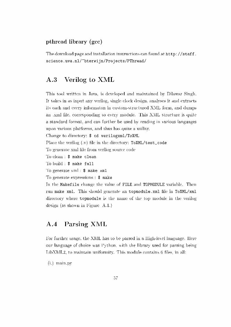
pthread library (gcc)
The download page and installation instructions can found at http://staff.
science.uva.nl/~bterwijn/Projects/PThread/
A.3 Verilog to XML
This tool written in Java, is developed and maintained by Dilawar Singh.
It takes in as input any verilog, single clock design, analyses it and extracts
its each and every informaton in custom-structured XML form, and dumps
an .xml �le, corresponding to every module. This XML structure is quite
a standard format, and can further be used by reading in various languages
upon various platforms, and thus has quite a utility.
Change to directory: $ cd verilogxml/ToXML
Place the verilog (.v) �le in the directory: ToXML/test_code
To generate xml �le from verilog source code
To clean : $ make clean
To build : $ make full
To generate xml : $ make xml
To generate expressions : $ make
In the Makefile change the value of FILE and TOPMODULE variable. Then
run make xml. This should generate an topmodule.xml �le in ToXML/xml
directory where topmodule is the name of the top module in the verilog
design (as shown in Figure A.1.)
A.4 Parsing XML
For further usage, the XML has to be parsed in a High-level language. Here
our language of choice was Python, with the library used for parsing being
LibXML2, to maintain uniformity. This module contains 6 �les, in all:
(i.) main.py
57
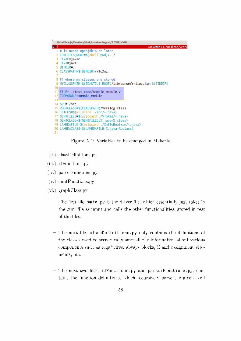
Figure A.1: Variables to be changed in Make�le
(ii.) classDe�nitions.py
(iii.) idFunctions.py
(iv.) parserFunctions.py
(v.) emitFunctions.py
(vi.) graphClass.py
� The �rst �le, main.py is the driver �le, which essentially just takes in
the .xml �le as input and calls the other functionalities, stored in rest
of the �les.
� The next �le, classDefinitions.py only contains the de�nitions of
the classes used to structurally save all the information about various
components such as regs/wires, always blocks, if and assignment stte-
ments, etc.
� The next two �les, idFunctions.py and parserFunctions.py, con-
tains the function de�nitions, which recursively parse the given .xml
58
�le and store all its information in the form of nested objects of the
classes described above.
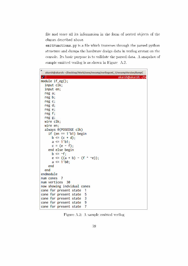
emitFunctions.py is a �le which traverses through the parsed python
structure and dumps the hardware design data in verilog syntax on the
console. Its basic purpose is to validate the parsed data. A snapshot of
sample emitted verilog is as shown in Figure A.2.
Figure A.2: A sample emitted verilog
59
� The last �le graphClass.py analyses the parsed verilog data in python
structure and makes a graph with regs, and wires and combinational
operators etc. as nodes and edges corresponding to their dependencies
on each other, at every clock cycle. It also generates the 'cones' (in
form of graphs) for each of �ip-�ops, which capture the combinational
dependency of each output's present state on its and other �ip-�ops'
previous state and constants. It also dumps all these graphs into stan-
dard .graphml format, which can easily be read by all graph libraries
for further usage. A Sample graph and a cone for a particular example
are as shown in Figure 7.1 and Figure 8.1 respectively.
To run this tool we need to just edit the name of the �le in main.py and
execute the same using
$ python main.py
A.5 Cones to Single assignment form expres-
sions
The cones dumped for each �ip-�op, in form of graph are then read and each
converted to their corresponding Single assignment form (SAF), list of ex-
pressions in the �le coneToSAF.py. It takes as input, list of all cones from the
�le all_cones.txt, which is dumped by the previous tool. It, then reads all
the cones' graphml �les and generates for each, a �le dump_expression_cone_num.txt
which contain their respective SAFs.
To run this, we just need to give the command:
$ python conesToSAF.py
For the taken example, the evaluated Single assignment form looks as shown
in Figure 10.2.
60
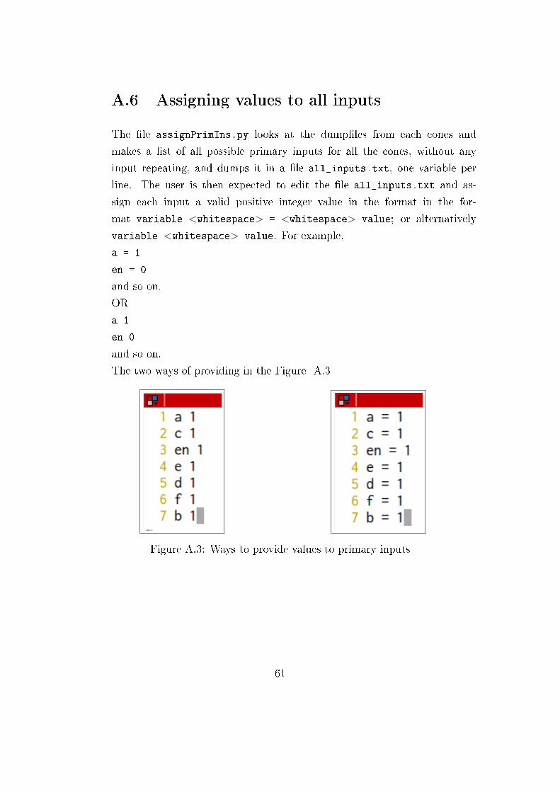
A.6 Assigning values to all inputs
The �le assignPrimIns.py looks at the dump�les from each cones and
makes a list of all possible primary inputs for all the cones, without any
input repeating, and dumps it in a �le all_inputs.txt, one variable per
line. The user is then expected to edit the �le all_inputs.txt and as-
sign each input a valid positive integer value in the format in the for-
mat variable <whitespace> = <whitespace> value; or alternatively
variable <whitespace> value. For example,
a = 1
en = 0
and so on.
OR
a 1
en 0
and so on.
The two ways of providing in the Figure A.3
Figure A.3: Ways to provide values to primary inputs
61
A.7 SAFs to individual thread functions
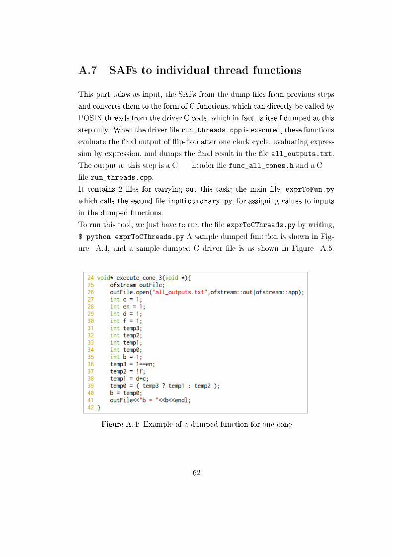
This part takes as input, the SAFs from the dump �les from previous steps
and converts them to the form of C functions, which can directly be called by
POSIX threads from the driver C code, which in fact, is itself dumped at this
step only. When the driver �le run_threads.cpp is executed, these functions
evaluate the �nal output of �ip-�op after one clock cycle, evaluating expres-
sion by expression, and dumps the �nal result in the �le all_outputs.txt.
The output at this step is a C++ header �le func_all_cones.h and a C++
�le run_threads.cpp.
It contains 2 �les for carrying out this task; the main �le, exprToFun.py
which calls the second �le inpDictionary.py, for assigning values to inputs
in the dumped functions.
To run this tool, we just have to run the �le exprToCThreads.py by writing,
$ python exprToCThreads.py A sample dumped function is shown in Fig-
ure A.4, and a sample dumped C driver �le is as shown in Figure A.5.
Figure A.4: Example of a dumped function for one cone
62
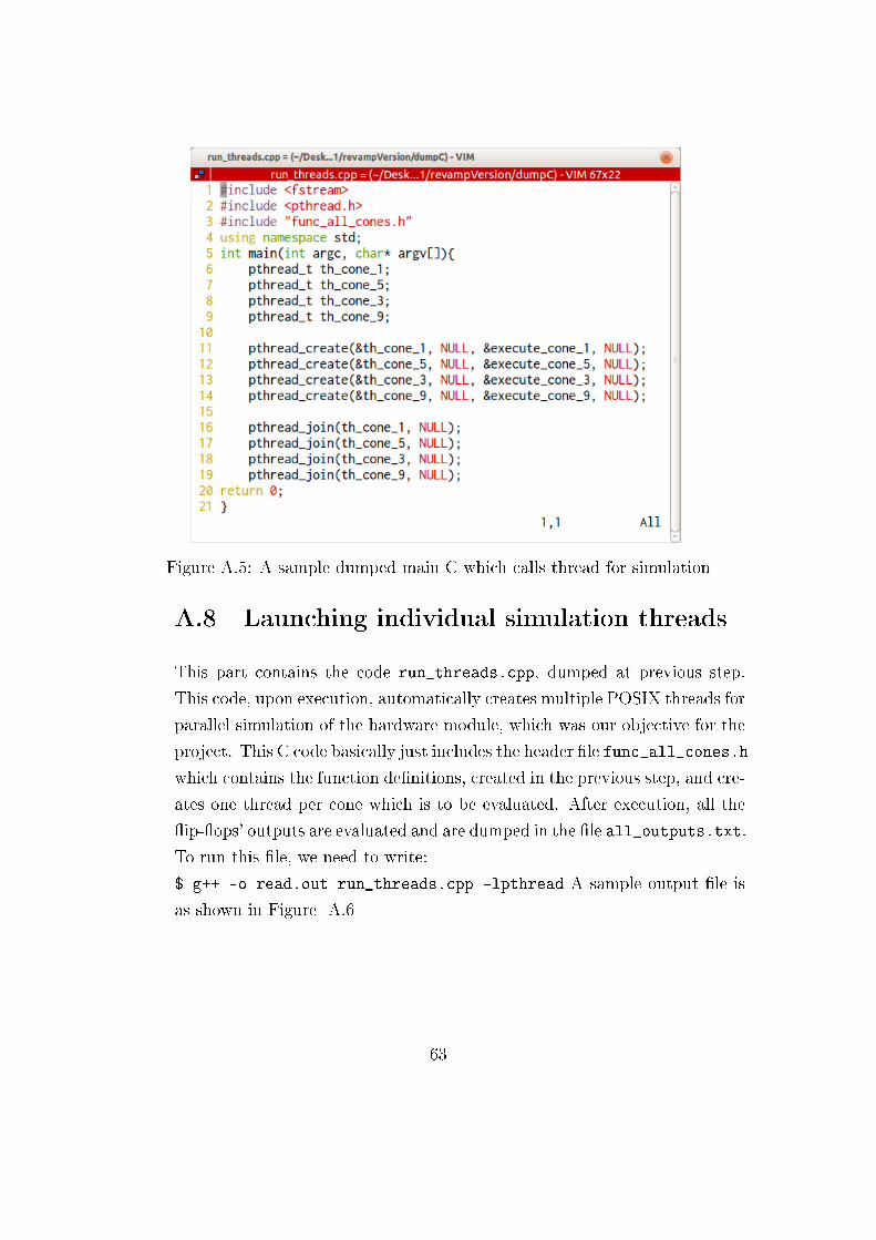
Figure A.5: A sample dumped main C which calls thread for simulation
A.8 Launching individual simulation threads
This part contains the code run_threads.cpp, dumped at previous step.
This code, upon execution, automatically creates multiple POSIX threads for
parallel simulation of the hardware module, which was our objective for the
project. This C code basically just includes the header �le func_all_cones.h
which contains the function de�nitions, created in the previous step, and cre-
ates one thread per cone which is to be evaluated. After execution, all the
�ip-�ops' outputs are evaluated and are dumped in the �le all_outputs.txt.
To run this �le, we need to write:
$ g++ -o read.out run_threads.cpp -lpthread A sample output �le is
as shown in Figure A.6
63

Figure A.6: Sample output for a set of FFs
64
Bibliography
[1] Giovanni De Micheli. Synthesis and optimisation of Digital Circuits. Tata
McGraw Hill, 2006
[2] Peter S. Pacheco. An Introduction to Parallel Programming. Elsevier,
2011
[3] Tiago de Paula Peixoto. Python Graph-tools library.
[4] Dilawar Singh. VerilogToXML library.
65