Parallel four-dimensional Haralick texture analysis for disk-resident image datasets

CONCURRENCY AND COMPUTATION: PRACTICE AND EXPERIENCEConcurrency Computat.: Pract. Exper. 2007; 19:65–87Published online 13 June 2006 in Wiley InterScience (www.interscience.wiley.com). DOI: 10.1002/cpe.1073

Parallel four-dimensionalHaralick texture analysis fordisk-resident image datasets

Brent Woods1, Bradley Clymer1, Johannes Heverhagen2,Michael Knopp2, Joel Saltz3 and Tahsin Kurc3,∗,†

1Department of Electrical and Computer Engineering,Ohio State University, Columbus, OH 43210, U.S.A.2Department of Radiology, Ohio State University, Columbus,OH 43210, U.S.A.3Department of Biomedical Informatics, Ohio State University,Columbus, OH 43210, U.S.A.

SUMMARY

Texture analysis is one possible method of detecting features in biomedical images. During textureanalysis, texture-related information is found by examining local variations in image brightness.Four-dimensional (4D) Haralick texture analysis is a method that extracts local variations along space andtime dimensions and represents them as a collection of 14 statistical parameters. However, application ofthe 4D Haralick method on large time-dependent image datasets is hindered by data retrieval, computation,and memory requirements. This paper describes a parallel implementation using a distributed component-based framework of 4D Haralick texture analysis on PC clusters. The experimental performance resultsshow that good performance can be achieved for this application via combined use of task- and data-parallelism. In addition, we show that our 4D texture analysis implementation can be used to classify imagedtissues. Copyright c© 2006 John Wiley & Sons, Ltd.

Received 25 October 2005; Revised 14 February 2006; Accepted 1 March 2006

KEY WORDS: biomedical image processing; texture analysis; distributed computing

∗Correspondence to: Tahsin Kurc, Department of Biomedical Informatics, Ohio State University, 3184 Graves Hall,333 West 10th Avenue, Columbus, OH 43210, U.S.A.†E-mail: [email protected]

Contract/grant sponsor: National Institute of Health (NIH) NIBIB BISTI; contract/grant number: P20EB000591Contract/grant sponsor: National Science Foundation; contract/grant numbers: ACI-9619020 (UC Subcontract 10152408),EIA-0121177, ACI-0203846, ACI-0130437, ANI-0330612 and ACI-9982087Contract/grant sponsor: Lawrence Livermore National Laboratory; contract/grant number: B517095 (UC Subcontract 10184497)Contract/grant sponsor: Ohio Board of Regents BRTTC; contract/grant number: BRTT02-0003

Copyright c© 2006 John Wiley & Sons, Ltd.

66 B. WOODS ET AL.

1. INTRODUCTION

The quality and usefulness of medical imaging is constantly evolving, leading to better patient careand more reliance on advanced imaging techniques. However, manual methods of analyzing largeimage datasets can be tedious and time-consuming for a researcher or clinician. In dynamic contrastenhanced magnetic resonance imaging (DCE-MRI), which is the motivating application for this paper,analysis methods often involve cinematic viewing of contrast agent flow, observation of a color-codedrepresentation of vascular permeability characteristics, and examination of the time versus signalintensity plots for individual pixels [1–3]. DCE-MRI involves repeated scans of the tissue under studyover several time steps, capturing a time-dependent sequence of three-dimensional (3D) image volumesin order to trace the diffusion of a contrast agent within the tissue of interest. Time-dependent imagesare also gathered in follow-up patient evaluations in order to monitor tumor volume. Extraction andanalysis of features from time-dependent medical images can be used to detect tumors and examinetheir progression over time.

In medical imaging, the diagnostic problem in the region of interest can often be associated with avariation in image brightness and texture [4,5]. During texture analysis, texture-related information isfound by examining local variations in image brightness. A form of statistical texture analysis describedby Haralick et al. [4] represents local variations as a collection of up to 14 statistical parameters, suchas contrast and entropy. Assisting the radiologist in extracting useful information from images usingtexture analysis can make it possible to have the results of the MRI procedure quickly, potentiallyreducing the overall analysis process from several days to hours, even to minutes. As advances inimaging technologies allow a researcher to capture higher quality images in a shorter period of time andacquire images over many time steps, the amount of data that must be stored and processed increases.Obtaining additional data by acquiring images over many time steps provides a more complete view ofthe patient’s physiology, but it can also create a quantity of data that may be impossible to process on asingle workstation. For example, high-resolution MRI scanners are capable of acquiring 3D volumes of1024× 1024 pixel images over many time steps. Also, texture analysis is a computationally intensiveprocess involving a series of matrix operations. Distributed computing can provide a solution to addressissues related to handling large datasets and executing computationally intensive operations efficiently.

We have developed a component-based middleware system that is designed to support processing ofvery large multidimensional scientific datasets [6–8]. The main contribution of our work is the efficientapplication of this middleware framework to develop a parallel implementation of four-dimensional(4D) Haralick texture analysis for disk-resident image datasets. Our approach involves combined useof task- and data-parallelism to leverage distributed computing power and storage space on PC clusters.Our experimental results show that the implementation is able to take advantage of distributed storageand computing power and to process large 4D datasets. This paper is an extended version of ourconference publication [9]. We present updated homogeneous and heterogeneous performance resultsfrom those described in the conference publication. We show in this paper new large-scale experimentswhere we efficiently process a 100 GB dataset. We also carry out a demonstration of how our 4D textureanalysis implementation can be used to segment out a malignant lesion from a DCE-MRI dataset.These new experiments are significant as they show that our implementation can efficiently processlarge datasets and that 4D texture analysis can be used for tumor detection. While our future goal inthis project is to evaluate the effectiveness of 4D texture analysis as a viable technique for analysisof biomedical images, in particular for DCE-MRI studies, the focus of this paper is the application of

Copyright c© 2006 John Wiley & Sons, Ltd. Concurrency Computat.: Pract. Exper. 2007; 19:65–87DOI: 10.1002/cpe

HARALICK TEXTURE ANALYSIS 67

a parallel middleware framework to speed up the execution of 4D Haralick texture analysis. The moreextensive evaluation of the efficacy of the analysis technique is under way and will be described in alater paper.

In Section 2 of this paper, we present background information regarding the DCE-MRI procedure,an overview of 4D texture analysis computations, and a discussion of related work in the field ofparallel image processing. In Section 3, we outline our design objectives and in Section 4 we discusshow our parallel 4D texture analysis system was implemented to achieve these objectives. In Section 5,we present performance analysis to show that execution speedup can be achieved in homogeneous andheterogeneous distributed computing environments. We also show that our implementation can handlevery large datasets and that 4D texture analysis has potential for use in tumor detection. Note thatSections 5.3 and 5.4 include new experiments that are an extension of our conference paper [9]. Finally,Section 6 provides a conclusion of our study.

2. BACKGROUND

In this section we describe the background information related to this study. In Section 2.1 we givean overview of the DCE-MRI procedure and describe current methods of DCE-MRI dataset analysis.In Section 2.2 we present the sequential 4D texture analysis algorithm. We discuss in Section 2.3related work in the field of parallel image processing.

2.1. DCE-MRI

DCE-MRI offers great potential in cancer diagnosis and tumor classification. The procedure may alsobe used to monitor the effectiveness of cancer therapies. During the DCE-MRI procedure, a contrastagent is used to study vascular permeability. A paramagnetic contrast agent, such as Gadolinium-DTPA, is administered intravenously [3]. Parenchymal (normal) tissue has a diffusion permeabilitycharacteristic that serves as a baseline. This baseline vascular permeability is compared with thevascular permeability of the tissue of interest to determine whether the tissue is non-malignant ormalignant, and if malignant, the diffusion characteristics can be used to classify the type of cancer.The contrast agent flows throughout the body with some making it to the region of the body beingimaged. Tumor tissue appears brighter than normal tissue when imaged by MRI because of thelocalized increase of the contrast agent. Repeated MRI scans occur until the body filters via the kidneysmost of the contrast agent from the blood stream. A time versus signal intensity curve is created foreach voxel in the volume.

The vascular permeability characteristics associated with certain tissues are summarized accordingto the pharmacokinetic two-compartment model. In the pharmacokinetic two-compartment model, timeversus signal intensity curves are used to quantify perfusion and vascular permeability. Widely usedproperties that can be obtained from the time-intensity curves include: amplitude (Amp), theredistribution rate constant (k21), and the elimination rate constant (kel) [2]. Large k21 and kel values, forinstance, are characteristic of malignant tissue. Figure 1 illustrates a sample time-intensity curve andthe vascular permeability characteristics for a voxel. From these parameters, radiologists differentiatenormal tissue from malignant tissue. Together, k21 and kel values can help radiologists predict leakiness


68 B. WOODS ET AL.

Figure 1. A sample time versus intensity plot showing Amp, K21, and kel parameters.

(a) (b)

Figure 2. Time versus intensity curves for (a) malignant tissue; (b) normal tissue.

of the vascular structures, which in turn helps radiologists classify tumors. Figure 2 illustrates time-intensity curves for malignant and non-malignant tissues.

Radiologists may examine the time-intensity curves for voxels in the volume. Another approachis to use computer-generated color-mapped images to classify the tissues being examined.The color-mapped images help radiologists find and classify tumors more quickly as vascular leakagecharacteristics are mapped to certain colors.

2.2. Four-dimensional Haralick texture analysis

The goal of texture analysis is to quantify the dependencies between neighboring pixels andpatterns of variation in image brightness within a region of interest [2,10,11]. In texture analysis,



Figure 3. The directions relative to the center pixel for 2D co-occurrence matrix calculation.

useful information can be found through examination of local variations in image brightness.Haralick texture analysis [4] is a form of statistical texture analysis that utilizes co-occurrence matricesto relay the joint statistics of neighboring pixels or voxels. The basis behind this method of textureanalysis is the study of second-order statistics relating neighboring pixels at various spacings anddirections. A second-order joint conditional probability density function is computed given a specificdistance between pixels and a specific direction. This second-order joint conditional probability densityfunction is referred to as a co-occurrence matrix. A co-occurrence matrix can also be thought of as ajoint histogram of two random variables. The random variables are the gray level of one pixel (g1)and the gray level of its neighboring pixel (g2), and the neighborhood between two pixels is definedby a user-specified distance and direction. This histogram gives the probability of neighboring pixelschanging from gray level g1 to g2.

There are several notable properties of the co-occurrence matrix. The relationships betweenneighboring pixels occur in both the forward and backward directions. Consider a two-dimensional(2D) case; there are eight total directions: 0, 45, 90, 135, 180, 225, 270, and 315 degrees. However,opposite angles yield the same co-occurrence matrix. Therefore, only four unique vectors exist(see Figure 3) for the eight possible directions. There is symmetry in the co-occurrence matrix becausethe gray level relationships between the pixels occur in both the forward and backward directions.The co-occurrence matrix is also a square matrix and is always Ng × Ng in size, where Ng is thetotal number of gray levels possible. Therefore, the size of the co-occurrence matrix is fixed by thetotal number of gray levels and is independent of distance and direction values. Once a co-occurrencematrix is computed, statistical parameters can be calculated from the matrix. The 14 textural featuresdescribed by Haralick et al. [4] provide a wide range of parameters that can be used in medical imaginganalysis.

In medical images, many localized texture changes denoting tumors, vessels, and differing tissuesmay exist. Thus, it is often necessary to apply a series of texture calculations with each calculation


70 B. WOODS ET AL.

Figure 4. A ROI window scans through the image creating a set of texture parameters at each movement.

R← (xl, yl , zl , tl) — ROI lengths in each direction.F ← {Hi, . . . , Hj }— Set of selected Haralick functions.

foreach x in (0, . . . , Lx − xl) doforeach y in (0, . . . , Ly − yl ) do

foreach z in (0, . . . , Lz − zl) doforeach t in (0, . . . , Lt − tl) do

ROI← (x, y, z, t)× (x + xl − 1, y + yl − 1, z + zl − 1, t + tl − 1)Mc← Compute co-occurrence matrix for ROI.foreach f in F do

Compute Haralick parameter f using Mc

Figure 5. Sequential 4D Haralick texture analysis algorithm.

performed on a localized region of interest. This process is known as raster scanning. Raster scanningbegins with a fixed, specified region of interest (ROI), where the size of the ROI depends on the size ofimportant structures within the image. Raster scanning begins at the first pixel (i.e. upper-left corner)in the image set. The region within the ROI window is used to generate a co-occurrence matrix. One ormore of the Haralick parameters are then calculated and sent to a storage buffer. The ROI windowis shifted to an adjacent voxel. Again, a co-occurrence matrix is generated based on data within theROI window. Haralick parameters are calculated and sent to a storage buffer. This scanning windowprocess continues for all points in which the ROI occurs within the boundary of the image. Figure 4illustrates raster scanning for the 2D case. The series of output parameters can be used in computer-aided diagnosis, stored to disk, or used to construct a graphical view of the results. Pseudo-codesummarizing the 4D Haralick texture analysis algorithm is given in Figure 5.



2.3. Parallel image processing

In this section, we present some of the previous work in parallel visualization and image analysis.Chiang and Silva [12] propose methods of iso-surface extraction for datasets that cannot fit inmemory. They introduce several techniques and indexing structures to search efficiently for cellsthrough which the iso-surface passes, reduce I/O costs, and reduce disk-space requirements. Cox andEllsworth [13] show that relying on operating system virtual memory results in poor performance.They propose a paging system with algorithms for memory management and paging for out-of-core visualization. Their results show that application-controlled paging can substantially improveapplication performance. Ueng et al. [14] present algorithms for streamline visualization of largeunstructured tetrahedral meshes. They employ an octree to partition an out-of-core dataset into smallersets, and they describe optimized techniques for scheduling operations and managing memory forstreamline visualization. Bajaj et al. [15] present a parallel algorithm for out-of-core isocontouring ofscientific datasets for visualization. In [15], several image-space partitioning algorithms are evaluatedon parallel systems for visualization of unstructured grids.

Manolakos and Funk [17] describe a Java-based tool for rapid prototyping of image-processingoperations. This tool uses a component-based framework, called JavaPorts, and implements a master-worker mechanism. Oberhuber [18] presents an infrastructure for remote execution of image-processing applications using NetSolve and SGI ImageVision library, which is developed to run onSGI machines [19]. Dv [20] is a framework for developing applications for distributed visualizationof large scientific datasets. It is based on the notion of active frames, which are application levelmobile objects. An active frame contains application data, called frame data, and a frame programthat processes the data. Active frames are executed by active frame servers running on the machinesat the client and remote sites. Hastings et al. [21] present a toolkit for distributed implementationand execution of image-analysis applications as a network of ITK (http://www.itk.org) and VTK(http://public.kitware.com/VTK) functions.

We are not aware of any parallel implementations of 4D Haralick texture analysis. Fleig et al. [22,23]implemented a parallel Haralick texture analysis program that worked on 2D slices of a 3D volume.Each slice was treated separately and processed by a single function in memory. Unlike the previousapproach, the implementation described in this paper handles disk-resident 4D datasets and can carryout texture computations in 4D.

3. DESIGN OBJECTIVES

One of our objectives is to develop an implementation of 4D Haralick texture analysis that can takeadvantage of aggregate memory space and computing power of high-performance machines usingdistributed computing. Another objective is to be able to handle disk-resident large image datasets usingdistributed storage clusters. To accomplish these objectives, we have modeled 4D Haralick textureanalysis as consisting of four major stages. The first stage reads in the 4D raw image dataset fromthe storage system and passes it to texture analysis operations. The second stage computes the co-occurrence matrices. The calculation of Haralick texture parameters from the co-occurrence matricesis the third stage in the processing structure. The resulting output is a 4D dataset for each textureparameter computed. The final stage outputs the 4D texture analysis results in a user-specified format.


72 B. WOODS ET AL.

Based on this modeling of Haralick texture analysis computations, we developed a task- and data-parallel implementation. Data parallelism is achieved by distributing data across the nodes in thesystem for both storage and computing purposes. The task parallelism is obtained by implementationand execution of the four major stages as separate tasks using a component-based framework calledDataCutter [6–8].

DataCutter is based on a filter-stream programming model that represents operations of a data-intensive application as a set of filters. Data are exchanged between filters using streams, which areunidirectional pipes. Streams deliver data from producer filters to consumer filters in user-defined datachunks (data buffers). To achieve distributed computing, operational tasks are divided among a seriesof filters. Each filter can be executed on a separate processor/machine in the environment, or filterscan be co-located on the same processor/machine. When filters are executed on separate machines,data exchange is done using TCP/IP sockets. When filters are co-located on the same machine, theruntime system transfers a data buffer from a producer filter to a consumer filter by copying the pointerto the data buffer. Consumer and producer filters can run concurrently and process data chunks ina pipelined fashion. Filters may be replicated and placed on different nodes. Data parallelism canbe made possible by distributing data buffers among replicated filters on-the-fly. Either explicit ortransparent copies of a filter can be instantiated and executed. If the copies of a filter are transparent, theDataCutter scheduler controls which of the identical filter copies receives a data buffer. The DataCutterscheduler can schedule data buffers to transparent filter copies in either round-robin or demand-drivensequences. In a round-robin distribution, the scheduler assigns data to each transparent filter in turn.In a demand-driven scheduling of data buffers, the DataCutter scheduler assigns the distribution basedon the buffer consumption rate of the transparent filter copies. The goal of the demand-driven approachis to send data to the transparent filter copies that can process them the fastest. Explicit filters are usedin situations where assignment of data chunks to filter copies in a user-defined way is required or canimprove performance.

4. SYSTEM DESCRIPTION

The implementation consists of a set of filters that are organized into a pipelined network of datareading, texture computing, and data output operations. We have developed three sets of filters tocarry out the four stages of Haralick texture analysis operations (see Figure 6). These filter sets canbe connected to form an end-to-end texture analysis application [24] (see Figure 7). The filters areimplemented in C++ using the base classes provided by the DataCutter framework and the filternetwork is expressed as an XML document [21]. In Section 4.1, we describe the filters implementedto achieve parallel 4D texture analysis. In Sections 4.2 and 4.3 we present optimizations involving theprocessing of sparse co-occurrence matrices and the reduction of network communication latencies.

4.1. Filters

4.1.1. RAWFileReader (RFR)

The purpose of the RFR filter is to read raw image data from disk and send them to other filtersfor processing. Multiple RFR filters can be executed if the image dataset is distributed across



Figure 6. Three filter sets carry out the main tasks in a Haralick texture analysis application.

(a) (b)

Figure 7. Example of two filter implementations: (a) input dataset is stored on a single file system, texture analysisoperations are combined in a single filter, and the texture parameters are output directly to disk; (b) input datasetis distributed among multiple storage systems, ROIs are constructed in the IIC filters, texture operations are splitinto two filters, texture parameter data are reconstructed, and texture parameters are stored to disk in JPEG format.

several storage nodes. In this case, an RFR filter is placed on each node containing image data.Each RFR filter extracts the local data needed to build a region of interest (ROI) and sends that data tothe input stitch filter. If all data are placed on a single node, the RFR filter may send data directly to thetexture analysis group.

4.1.2. InputImageConstructor (IIC) (Input Stitch)

In order to compute a co-occurrence matrix, the complete ROI data are needed. If the 4D image datasetis distributed across multiple storage nodes, then a copy of the RAWFileReader filter will retrieve andsend only the local data portions to the filter in the next stage. The InputImageConstructor (IIC) filterreconstructs full ROIs and distributes them to the texture analysis filters. The inputs to the IIC filter areportions of the image data from the output of different RFR filters. The IIC filter places the input MRIportions into temporary buffers. After all data elements needed to build a complete ROI are received,


74 B. WOODS ET AL.

the ROI is put into a send buffer. When the send buffer is full, the buffer data are sent to the textureanalysis filters.

In our implementation, the texture analysis algorithm can be carried out in a distributed environmentin various ways. The texture analysis operations for computing co-occurrence matrices and Haralickparameters can be contained in a single filter or task-distributed among two pipelined filters.Dividing the operations among two filters creates another level of task parallelism, but also introducescommunication overhead between the filters that perform the operations.

4.1.3. HaralickMatrixAndParameter (HMP)

The HMP filter carries out the entire texture-analysis processing. The filter receives a buffer of ROIimage data from an IIC or RFR filter, depending on whether or not the input dataset is distributed amongmultiple nodes. For each of the ROIs in the input buffer, a co-occurrence matrix is calculated basedon the image data within the ROI. The co-occurrence matrix is then used to generate user-selectedHaralick parameters.

4.1.4. HaralickCoMatrixCalculator (HCC)

The HCC filter is responsible for calculating just the co-occurrence matrices from the input data.For each ROI in the input buffer, a co-occurrence matrix is calculated. The co-occurrence informationis stored in an output buffer. When the output buffer becomes full or the end of an input data message isreceived, the co-occurrence matrices in the output buffer are passed to the HaralickParameterCalculatorfilter.

4.1.5. HaralickParameterCalculator (HPC)

The HPC filter is responsible for calculating the Haralick parameters from the co-occurrence matricesreceived from an HCC filter. All user-selected Haralick parameters are calculated for each matrix.Each parameter is stored in its own output buffer. When the output buffers are full or when the end ofan input data message is encountered, the data elements stored within the output buffers are sent to anoutput filter.

The user may choose to send the output portions received from the texture analysis filters directly todisk. Once on disk, the data may be postprocessed for purposes of computer-aided diagnosis. The usermay also choose to store the Haralick parameter results in a visual way. To accomplish this, Haralickparameter output portions sent from the texture analysis filters are received at an output stitch filter.This filter reconstructs the parameter output portions into a series of 4D datasets. Each 4D dataset isthe output for a single Haralick parameter. Once reconstructed, the 4D output datasets can be writtento disk as a series of JPEG images or raw floating point values.

4.1.6. UnstitchedOutput (USO)

The USO filter is responsible for writing the Haralick parameter information out to disk. The input tothis filter is a stream of data elements for a Haralick parameter. Each input stream is assigned a uniquefile name. A file is opened, and the parameter values along with corresponding positional information



are stored to the file. Postprocessing applications can then use the data stored in these files for furthercomputations.

4.1.7. HaralickImageConstructor (HIC)

The HIC filter is used to build the Haralick parameter information into images. This filter receives inputstreams consisting of Haralick parameter information. Each input stream contains a subset of the totaloutput elements for a single Haralick parameter. The output stitch filter uses positional informationstored in the input stream to place the parameter elements into their appropriate positions in theparameter image data structure. Once all data elements for a Haralick parameter have been placedcorrectly, a 4D dataset consisting of all elements for a parameter has been built. The complete 4Ddataset is then sent to another filter for further processing and/or storage.

4.1.8. JPGImageWriter (JIW)

The JIW filter receives a stream of data containing elements for a Haralick parameter dataset that havebeen assembled by position. The input stream also contains the minimum and maximum values for theHaralick parameter elements. Using the minimum and maximum values, the data can be normalized.The filter then converts the 4D data into a series of 2D images that are stored in JPEG format. The JIWfilter may be configured to store the raw floating point data to disk as well.

Transparent filter copies of the RFR, HMP, HCC, HPC, and USO filters can be instantiated andexecuted in the environment. Copies of the IIC and HIC filters may be instantiated where each filteris responsible for an explicit portion of the input or output dataset. Figure 7 shows two possibleinstantiations.

4.2. Performance optimization 1: full versus sparse matrix representation

The co-occurrence matrix relates the intensities of neighboring pixels along a certain direction.The number of gray levels (Ng) may be relatively large, such as 65 536 (16-bit) intensity levels, orrelatively small, such as requantized 32 (5-bit) levels. Our experiments have shown that in some cases,matrices generated using a typical 5× 5× 5× 5 ROI and requantized 32 levels can have, on average,as few as 11 non-zero entries per matrix (out of 1024 entries, about 1% of the matrix). Note thatthis average takes into account matrix symmetry, and the symmetric entries are only counted once.Knowing that many of the co-occurrence matrices are relatively sparse leads us to the following matrixstorage schemes and optimizations.

The most obvious method of representing a co-occurrence matrix in memory is a 2D array ofNg ×Ng elements. Without optimization, all Haralick parameter calculations treat each element inthe matrix the same. Therefore, both zero entries and non-zero entries in the matrix result in additionsto running sums. However, before operating on an entry from the co-occurrence matrix, the entry canbe tested to see if it is zero. If the entry is zero valued, then the entry is simply skipped. By firstchecking for zero values, we are able to reduce the time needed to process relatively sparse matrices.In fact, this optimization allows us to process a typical MRI dataset in up to one-fourth of the time.We refer to this representation as the full matrix storage representation. The co-occurrence matrixmay also be stored in a sparse matrix storage representation. Only the non-zero and non-duplicated


76 B. WOODS ET AL.

(due to symmetry) entries are stored along with positional information in memory. The positionalinformation is needed to map each non-zero, non-duplicated entry to its position in the co-occurrencematrix. If a matrix is in the sparse form, then the Haralick parameter calculations do not have to checkfor non-zero entries. Therefore, the matrix can be processed directly from the sparse form, and noconversion back to a 2D Ng ×Ng array is needed. In addition, the sparse matrix representation cangreatly reduce the data traffic leaving the HCC filters, as the matrices are also transmitted to the HPCfilters in the sparse form via the network.

The level of co-occurrence matrix sparsity depends on several factors. The number of total graylevels affects the overall size of the Ng × Ng array. Therefore, it is possible for a 16× 16 array tohave a higher percentage of non-zero elements compared to a 256× 256 array. Also, the size of theROI affects sparsity as the number of voxels within the ROI limits the number of gray level transitionspossible. For example, a large 256× 256× 16× 16 ROI will probably have more gray level transitionsthan a smaller 5× 5× 5× 5 ROI. The amount of homogeneity of the voxels within the ROI can alsoaffect matrix sparsity. Typically, the tissue being analyzed has smooth and gradual voxel intensitychanges that contribute to a sparse matrix. However, noise in the image and blurred edges of structuresin the image can lead to a wider variety of voxel intensity change and a dense matrix.

For our DCE-MRI analysis, the sparse matrix optimization will probably always be used. This isbecause the 32× 32 array is larger than the total number of gray level transitions possible within a ROI.Also, there is a high degree of gray level homogeneity within the ROIs of the images. We can, however,produce contrived examples that illustrate cases where using the full matrix representation gives betterresults than the sparse matrix representation. For example, when using the HMP implementation, ifthe co-occurrence matrix is on average greater than 31% filled (not accounting for symmetry), thenthe full matrix representation should be used. When using the HCC+ HPC implementation, if the co-occurrence matrix is on average greater than 26% filled (accounting for symmetry), then the full matrixrepresentation should be used. Note that communication latencies play an important role in choosingwhen and when not to use the sparse matrix representation with the HCC+ HPC implementation.

4.3. Performance optimization 2: reducing I/O and communication volume

Complete 4D ROI data are necessary to build one co-occurrence matrix. Figure 8(a) illustrates how a2D image can be accessed by ROIs; thus, each data packet sent to the texture analysis filters containsthe ROI needed to build a single co-occurrence matrix. In Figure 8(a), ROIx and ROIy correspond tothe dimension lengths of the ROI, which are supplied by the user. Also in Figure 8(a), P1, P2, and P3are the data chunks sent to the texture analysis filters. Note that most of the chunks contain overlappingdata. If the input data are retrieved by ROIs, the data elements in the overlapped regions must beretrieved and sent to the texture analysis filters multiple times. Therefore, data retrieval in terms ofROIs creates the largest volume of communication between the input filters and the texture analysisfilters. In order to reduce the amount of data read from disk and communicated between RFR and IICfilters as well as IIC and texture analysis filters, the data are retrieved in 4D chunks, each of whichcontains a subset of ROIs. In Figure 8(b), a 2D image is partitioned into four data chunks each withthe user-specified dimensions, chunkx × chunky . The amount of overlap between two chunks in thex direction depends on the ROI x dimension length, and the amount of overlap between two adjacentchunks in the y direction depends on the ROI y dimension length.

The current implementation has two types of data chunk: an RFR-to-IIC chunk for data retrievedfrom disk and sent to the IIC filter and an IIC-to-TEXTURE chunk for communication between the IIC



For Peer R

(a) (b)

Figure 8. Two data retrieval strategies: (a) retrieving ROIs; (b) retrieving chunks.

and texture analysis filters. The input image data are stored as a set of image slices on disk. An RFRfilter reads a 2D subsection of each image slice and puts it into a buffer, which corresponds to the I/Ochunk. When the buffer is full, the RFR filter sends the buffer to the IIC filter. When the IIC filterreceives buffers from RFR filters, it copies and reorganizes the contents of the buffers into a set ofoutput buffers, each of which is a 4D array and corresponds to a separate IIC-to-TEXTURE chunk.When a buffer is full, it is sent to one of the copies of the texture analysis filters (i.e. HMP or HCCfilters).

Having two types of chunk allows better optimization of execution time for different types ofoverhead. The RFR-to-IIC chunk dimensions may be chosen depending on how the dataset isdistributed on disk so that disk-seek operations are minimized. If the IIC filter can process an incomingchuck quickly, then RFR-to-IIC chunk size may be kept small in order to keep each IIC filter busy.Similarly, with a smaller size for the IIC-to-TEXTURE chunk, pipelining between the IIC and textureanalysis filters can be increased. However, using smaller IIC-to-TEXTURE chunks leads to a highertotal communication volume as data in the overlapping areas must be sent across the network multipletimes. Thus, communication latencies play an important role in choosing optimal chunk sizes.

5. RESULTS

In this section, we report on the performance of our implementation and demonstrate how ourimplementation may be used for tissue classification. The first set of experiments (Section 5.1)examines the performance impact of the full versus sparse matrix representation and the trade-offs of using various filter configurations in a homogeneous computing environment. In the secondset of experiments (Section 5.2), we show how pipelining and buffer-scheduling policies influence


78 B. WOODS ET AL.

performance of our implementation in a heterogeneous computing environment. The third set ofexperiments (Section 5.3) shows the ability of our implementation to handle large datasets andsubregions. Finally, in Section 5.4, we demonstrate how DCE-MRI texture analysis results may beused in a tissue classification system.

5.1. Homogeneous cluster experiments

For the experiments on homogeneous and heterogeneous systems, we use a dataset obtained from aDCE-MRI study. This dataset consists of 32 time steps where each time step is made up of 32 imagesof 256× 256 pixels each. Each pixel is 2 bytes in size. Dataset sizes influence execution time and thedimension lengths may vary as long as they are larger than the ROI dimension lengths. Factors suchas co-occurrence matrix sparseness can vary by the patient being imaged. Ideally, we would liketo examine the performance of our system using different datasets. However, the DCE-MRI studiesavailable are all similar in terms of size and average co-occurrence matrix sparseness. Thus, we choseone specific dataset for our homogenous and heterogeneous experiments. To investigate the effect oflarger datasets on the performance of our system, we used larger datasets in the experiments presentedin Section 5.3.

For the experiments in this section, 2D image slices that contribute to a 3D volume at a time stepwere distributed across four storage nodes in round-robin fashion. Each 2D image was assigned to asingle storage node and stored on disk in a separate file. A simple index file was created on each storagenode, and each index file contains a (slice number, time step) tuple for each image file on the storagenode. Other data distribution strategies were tested [24] but not included in this paper because of spaceconstraints.

The ROI was set according to the dimension lengths 5× 5× 5× 5 because previous studies on theanalysis of 2D images showed that such a ROI would be typical for an MRI application. The numberof gray levels used to re-quantize the DCE-MRI dataset was set to 32, because, in most cases,using more than 32 gray levels does not significantly improve the texture analysis results [2,25].For experimental performance evaluation purposes, the following Haralick parameters were calculated:angular second moment, correlation, sum of squares, and inverse difference moment [4], which are themost computation-intensive parameters.

Because each image slice in the input dataset is relatively small, the RFR-to-IIC chunk dimensionlengths were set to 256× 256× 6× 6. In this way, a RFR filter can read one image slice withoutany disk-seek operations required to retrieve smaller image regions. The IIC-to-TEXTURE chunkdimension lengths used in data partitioning for distribution to texture analysis filters were set to67× 67× 6× 6 for all tests. When we conducted tests using smaller chunks, the overlap betweenpartitions created a volume of communication that was too great. As a result, the program executiontime was very large. Larger chunk sizes also produced poor results because the large data portionscould not be distributed to the texture analysis filters fast enough, leaving some texture analysis filtersin an idle state. Therefore, we chose a chunk size that had a tolerable amount of overlap as a result ofpartitioning and also produced balanced data distribution among the texture analysis filters. The HCCfilters were configured to send out a packet of co-occurrence matrices whenever 1/64 of a chunk hadbeen processed. For our configuration these settings result in good pipelining of data across differentstages of the filter groups, but do not cause excessive communication latencies.

For the experiments detailed in this section, a homogeneous PC cluster was used. The cluster,referred to here as PIII, contains 24 nodes, each with a Pentium III 900 MHz processor and



(a) (b)

Figure 9. The two filter layouts tested. (a) Texture analysis operations are combined in the HMP filter. The numberof HMP filters is varied to test performance. (b) Texture analysis operations are split among the HCC and HPC

filters. The number of HCC and HPC filters is varied to test performance.

512 MB of memory. All nodes are connected via a FastEthernet Switch capable of transmitting data ata rate of 100 Mbits/s.

In the first set of experiments, we investigate the impact of using full matrix representation versussparse matrix representation and the performance of the split HCC and HPC filter implementationand the HMP filter implementation. The input dataset was distributed across four nodes, so four RFRfilters were used. One of the nodes in the cluster was used to run the IIC filter, and one USO filterwas used for output. The remaining nodes were used to run the HMP filters or the HCC and HPCfilters (see Figure 9). Figure 10(a) shows the execution time when the number of transparent HMPfilters (each on its own node) is varied from one to 16. Note from Figure 10(a) that the sparse matrixrepresentation performs better than the full matrix representation. The percentage improvement fromthe HMP full matrix to the HMP sparse matrix implementation is: 26.95% average, 0.86% minimum,and 37.41% maximum. There is an initial overhead from storing the matrices in sparse representation.However, this overhead is small compared to the performance benefit resulting from the need to processonly a small portion of the Ng ×Ng matrix entries. Similarly, using the sparse matrix representationachieves better performance in the split HCC and HPC filter case, as shown in Figure 10(b). However,the performance benefit is much greater in this case because, with the sparse representation, thecommunication overhead is reduced significantly. The percentage improvement from the HCC+ HPCfull matrix to the HCC+ HPC sparse matrix implementation is: 75.09% average, 58.62% minimum,and 84.91% maximum. Multiple transparent copies of the HCC and HPC filters are created, but onlyone filter is executed on one node. Note that, for the one-node configuration, both HCC and HPCfilter copies are executed on the same node. The number of copies of the HCC and HPC filters wasdetermined based on their relative processing times. We observed that the HCC filter was on averageabout five to six times more expensive than the HPC filter. Hence, the number of nodes in a given setupwas partitioned so that an approximate five-to-one ratio was maintained between the HCC and HPCfilters. For example, in the 16-node configuration, 13 HCC and three HPC filters were executed.


80 B. WOODS ET AL.

eer

0

2000

4000

6000

8000

10000

12000

1 2 4 8 16

Number of Processors

Ex

ecu

tio

nT

ime

(seco

nd

s)

HMP Full

HMP Sparse

eer

0

2000

4000

6000

8000

10000

12000

1 2 4 8 16


Ex

ecu

tio

nT

ime

(seco

nd

s)

HMP Full

HMP Sparse

(a) (b)

Figure 10. The performance impact of using full matrix representation versus sparse matrix representation: (a) theHMP filter implementation; (b) the split HCC+ HPC filter implementation.r

0

1000

2000

3000

4000

5000

6000

7000

1 2 4 8 16


Execu

tio

nT

ime

(seco

nd

s)

HCC+HPC No Overlap

HPC+HCC All Overlap

HMP

Figure 11. The performance impact of co-locating HCC and HPC filters versusrunning them on separate processors.

The split HCC and HPC filter implementation provides flexibility in that HCC and HPC filters canbe executed on separate nodes or run on the same node. The next set of experiments examines theperformance impact of executing copies of HCC and HPC filters on the same node. When HCC andHPC filters are placed on the same node, the communication overhead is reduced, as buffers from theHCC filter that are delivered to the local copy of the HPC filter incur no communication overhead(buffer exchange between two co-located filters is done via a pointer copy operation). In addition,more copies of the HCC and HPC filters can be executed in the system. However, because a nodein the PIII cluster has a single processor, the CPU has to multiplex between the two filters and itspower has to be shared. In Figure 11, No Overlap denotes the case in which no two filters are co-located, whereas copies of the HCC and HPC filters are executed on the same node in the Overlap case.



Review0

1000

2000

3000

4000

5000

6000

1 2 4 8 16


Execu

tio

nT

ime

(seco

nd

s)

RFR

IIC

HCC

HPC

USO

Figure 12. The processing time of each filter in the split HCC and HPC filter implementation. HCCand HPC filters are executed on separate nodes.

In the experiments, the HMP filter implementation and the split HCC and HPC filter implementationemploy the sparse matrix representation for co-occurrence matrices. As shown in Figure 11, Overlapachieves better performance compared to the HMP filter implementation and the No Overlap HCC+HPC implementation. The percentage improvement from the No Overlap HCC+ HPC to the OverlapHCC+ HPC implementation is: 26.47% average, 15.96% minimum, and 49.50% maximum. Althoughthe processing power is shared between two filters, the reduction in communication overhead and morecopies of the filters result in better performance. We also observe that in the one-node case, the splitHCC and HPC filter implementation performs better than the HMP filter implementation. This resultcan be attributed to better pipelining achieved by the split implementation; when an HCC or HPC filteris waiting for send and receive operations to complete, the other filter can be doing computations.

Figure 12 shows the processing time of each filter (RFR, IIC, HCC, HPC, and USO) for the splitHCC and HPC filter implementation. The read (RFR) and write (USO) overheads are negligiblecompared to the time taken by other filters. We observe that the execution time of the HCC andHPC filters decreases as more nodes are added. The IIC filter becomes a bottleneck in the 16-nodeconfiguration and adversely affects the scalability to a larger number of nodes. In order to alleviate thisbottleneck, multiple explicit copies of the IIC filter can be instantiated. Explicit (rather than transparent)IIC filter copies must be executed because each IIC filter is responsible for building data chunks fora specific portion of the overall dataset. As the number of IIC filters is increased, the processing timeof each IIC filter decreases almost linearly, as expected. Another solution is to remove the IIC filteraltogether by replicating the input data so that local RFR filters can always build complete data chunks.This strategy removes the need for IIC filters, but replicating large amounts of data on disk may notalways be possible.

As discussed in Section 4.2, factors such as ROI size and variations in voxel intensities withinthe image dataset influence whether or not to use the sparse matrix optimization. When thefull matrix optimization is used, the HMP implementation performs better (see Figure 10).The percentage improvement from the HCC+ HPC full matrix implementation to the HMP full matrix


82 B. WOODS ET AL.

implementation is: 67.47% average, 26.95% minimum, and 80.97% maximum. Communication of thefull co-occurrence matrices across a network masks any benefits from pipelining in the HCC+ HPCimplementation.

When the sparse matrix optimization is used, the HMP implementation performs better than the NoOverlap HCC + HPC implementation and worse than the All Overlap HCC+ HPC implementation(see Figure 11). Specifically, the percentage improvement from the No Overlap HCC+ HPC sparsematrix implementation to the HMP sparse matrix implementation is: 16.65% average, 0.50% minimum,and 42.78% maximum. This is due to communication overhead between the HCC and HPC filters andalso to load imbalance as the HCC filter takes longer to process a chunk of data compared to theHPC filter (see Figure 12). The All Overlap HCC+ HPC implementation performs better than theHMP implementation. The percentage improvement from the HMP sparse matrix implementation tothe All Overlap HCC+ HPC sparse matrix implementation is: 11.39% average, 2.72% minimum, and16.37% maximum. Under the All Overlap HCC + HPC implementation load balance and pipeliningare achieved, and this implementation achieves best performance for our dataset under the conditionsof the experiment. Note that when the number of processors is increased, execution time and thusperformance of the texture analysis stage is influenced by overheads and bottlenecks associatedwith the RFR, IIC, and USO filters. However, the effectiveness within the texture analysis stage(HMP, HCC, and HPC) remains about the same as described above.

5.2. Heterogeneous environment experiments

In this set of experiments, we investigate execution of the parallel implementation in a heterogeneousenvironment. In addition to the PIII cluster used in the homogeneous experiments, two additionalclusters are employed. The first additional cluster, referred to here as XEON, contains five nodes.Each node of the XEON cluster has dual Xeon 2.4 GHz processors and 2 GB of memory. The nodeson the XEON cluster are connected by a Gigabit switch. The second additional cluster, referred to hereas OPTERON, contains six nodes. Each node of the OPTERON cluster has dual Opteron 1.4 GHzprocessors and 8 GB of memory. The nodes of the OPTERON cluster are also connected by a Gigabitswitch. PIII is connected to XEON and OPTERON through a shared 100 Mbit/s network. XEON andOPTERON are connected to each other using a Gigabit Switch.

Two experiments were performed to test the implementations in a heterogeneous environment.The first experiment provides a comparison of the HMP filter implementation and the split HCC andHPC filter implementation using the PIII and XEON clusters. In this experiment, four RFR filters,four IIC filters, and two USO filters were executed on the PIII cluster. The texture analysis filters wereplaced across the two clusters on a total of 18 nodes (13 nodes from the PIII cluster and five fromthe XEON cluster). For the HMP filter implementation, one transparent copy of the HMP filter wasinstantiated on each processor. Because the XEON cluster has ten processors (on five nodes), the totalnumber of HMP filters was 23. For the split HCC and HPC filter implementation, one copy of HCCand one copy of HPC were co-located on each node, which resulted in 18 copies of the HCC and18 copies of the HPC filters. While the HMP filter implementation aims to achieve good performanceby spreading data across more HMP filters, the split HPC and HCC implementation targets a morebalanced use of task- and data-parallelism by splitting the co-occurrence matrix computations andHaralick parameter calculations. As shown in Figure 13, the HCC + HPC implementation achieves a5.43% increase in performance over the HMP implementation. Firstly, although ten copies of the HMP



or Peer290

295

300

305

310

315

320

325

HMP HCC+HPC

Implementation

Execu

tio

nT

ime

(seco

nd

s)

Figure 13. Performance comparison of the heterogenous HMP filter implementation and thesplit HCC+ HPC filter implementation.

filter can be created on the XEON cluster, more data has to flow from the PIII cluster to this clusteracross a relatively slow network to make optimal use of these copies. Conversely, the split HCC andHPC filter implementation can take advantage of demand-driven scheduling of co-occurrence matrixbuffers across the filters within the same cluster. Secondly, better pipelining of computations and betteroverlap between computation and communication can be achieved with the split HCC and HPC filterimplementation, especially on the XEON cluster where the HCC and HPC filters are co-located on thesame node but are run on separate processors.

In the second heterogeneous experiment, the XEON and OPTERON clusters were used to compareround-robin and demand-driven buffer-scheduling policies. Four RFR filters, one IIC filter, two HPCfilters, and one USO filter were executed on separate nodes of the OPTERON cluster. Because the HCCfilter is the most computation-expensivefilter, the HCC filters were used to evaluate the round-robin anddemand-driven scheduling-policies. Four HCC filters were placed on the XEON nodes and four HCCfilters were placed on the OPTERON nodes. In this filter layout no more than one filter is assignedto any processor. When using the round-robin mechanism, the DataCutter scheduler assures that alltransparent filter copies receive approximately the same number of data buffers. The demand-drivenmechanism allows the DataCutter scheduler to assign data buffers to the transparent consumer copythat is likely to process data the fastest. As shown in Figure 14, the demand-driven method achieves a35.06% increase in performance over the round-robin method. Filter placement also becomes importantwhen using the demand-driven policy. Because the OPTERON HCC filters receive more data packetsin demand-driven scheduling, there is less communication overhead because the HPC filters are alsoplaced on the OPTERON nodes. In this experiment, the round-robin scheduling method causes theXEON HCC filters to receive more data packets; therefore, more HCC-HPC communication overheadexists compared with the demand-driven method.

The homogeneous and heterogeneous experiments show that factors such as network bandwidthplay an important role in choosing the implementation to use, filter layout, and sizes of buffers usedfor transferring data between two filters. For example, if network latency is high and bandwidth is low,


84 B. WOODS ET AL.

R

0

100

200

300

400

500

600

700

800

Round Robin Demand Driven

Buffer Scheduling Method

Ex

ec

uti

on

Tim

e(s

ec

on

ds

)

Figure 14. Performance comparison of the round-robin and demand-driven buffer scheduling policies.

communication overhead incurred by transmitting small buffers can outweigh the gain from morepipelining. In such a case, larger buffers might achieve better performance results. Furthermore, filtersthat exchange large volumes of data can be co-located to minimize communication volume.

5.3. Large-scale experiments

This experiment illustrates our implementation’s ability to process a very large dataset and subregionsof the dataset. We process first the dataset in its entirety and then process two different sized subregionsof the dataset. The large dataset is a 100 GB scaled DCE-MRI breast cancer study of dimensions8192× 8192× 28× 28 and 2 bytes/pixel. The first subregion is the breast tissue (neglecting air) andeight time samples only. This 14 GB dataset of dimensions 8192× 4096× 28× 8 contains only thebreast tissue. Such a subregion is useful when the location of the breast in the image set is known, butthe general location of tumor tissue is unknown. Eight time samples are enough for tissue classificationas long as the samples include a balance of baseline, contrast uptake, and contrast elimination scans.The second subregion focuses on a portion of the volume containing tumor tissue and eight timesamples. This dataset is 1.1875 GB in size and of dimensions 2048× 2048× 19× 8. Focusing onsuch a small region is useful in cases where the approximate location of the tumor is known and thevolume of the tumor is being monitored during a cancer therapy. All regions were processed on thePIII cluster and 22 total processors were used (16 for texture analysis). The HCC and HPC filters wereco-located, and the RFR (×4) and USO (×4) filters were also co-located. In addition, two IIC filterswere used to avoid bottlenecks in that stage of processing. Figure 15 shows a 99.06% reduction inexecution time as we zoom in from a full dataset to a specific subregion around the tumor. The resultsdemonstrate the following.

• Our implementation can handle very large datasets.• Execution time reduces as the subregion to be retrieved and processed becomes smaller. That is,

the execution time is proportional to the size of the subregion, not to the size of the entire dataset.



w0

10

20

30

40

50

60

70

80

90

100

Full Dataset Breast Tissue And

8 Time Samples

Tumor Region And

8 Time Samples

To

tal

Ex

ec

uti

on

Tim

e(H

rs)

Figure 15. Execution times for specific subregions of a very large dataset.

5.4. Tissue classification results

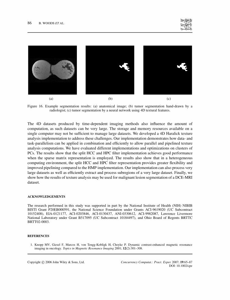
The tissue classification results for an intra-lobular breast cancer study are outlined in this section.For the breast cancer study, a neural network was trained using selected Haralick texture analysisparameters and radiologist marked images to determine whether or not a voxel should be classifiedas malignant tissue. The training set was selected from approximately 10% of voxels in the study forwhich there was at least moderate contrast change. Once trained, each voxel in the breast cancer studywas classified based on its associated textural parameters. The output was then compared with theexpected results provided by the radiologist.

Figure 16 shows the neural network classification results as compared with the radiologist-markedregions for a particular image slice. 4D texture analysis along with a neural network shows potentialfor detecting malignant tissue in DCE-MRI datasets. There are several circumstances when such aclassification system can be used effectively. Firstly, we consider a patient known to have cancer.In order to monitor the effectiveness of the cancer therapy, the patient can undergo several DCE-MRIprocedures over weeks of treatment. It may be possible for the radiologist to use the tissue classificationtechnique presented in this paper to automatically or semi-automatically calculate tumor volume inorder to monitor the effectiveness of cancer therapies. Another possible use for the system is to giveradiologists an initial approximation of the tumor’s type, size, and location. A future paper will detailthe classification system and tissue classification performance for a larger range of studies.

6. CONCLUSIONS

Haralick texture analysis is a computationally intensive application that involves repeatedco-occurrence matrix generation and repeated computations on the co-occurrence matrices.


86 B. WOODS ET AL.

(a) (b) (c)

Figure 16. Example segmentation results: (a) anatomical image; (b) tumor segmentation hand-drawn by aradiologist; (c) tumor segmentation by a neural network using 4D textural features.

The 4D datasets produced by time-dependent imaging methods also influence the amount ofcomputation, as such datasets can be very large. The storage and memory resources available on asingle computer may not be sufficient to manage large datasets. We developed a 4D Haralick textureanalysis implementation to address these challenges. Our implementation demonstrates how data- andtask-parallelism can be applied in combination and efficiently to allow parallel and pipelined textureanalysis computations. We have evaluated different implementations and optimizations on clusters ofPCs. The results show that the split HCC and HPC filter implementation achieves good performancewhen the sparse matrix representation is employed. The results also show that in a heterogeneouscomputing environment, the split HCC and HPC filter representation provides greater flexibility andimproved pipelining compared to the HMP implementation. Our implementation can also process verylarge datasets as well as efficiently extract and process subregions of a very large dataset. Finally, weshow how the results of texture analysis may be used for malignant lesion segmentation of a DCE-MRIdataset.

ACKNOWLEDGEMENTS

The research performed in this study was supported in part by the National Institute of Health (NIH) NIBIBBISTI Grant P20EB000591, the National Science Foundation under Grants ACI-9619020 (UC Subcontract10152408), EIA-0121177, ACI-0203846, ACI-0130437, ANI-0330612, ACI-9982087, Lawrence LivermoreNational Laboratory under Grant B517095 (UC Subcontract 10184497), and Ohio Board of Regents BRTTCBRTT02-0003.

REFERENCES

1. Knopp MV, Giesel F, Marcos H, von Tengg-Kobligk H, Choyke P. Dynamic contrast-enhanced magnetic resonanceimaging in oncology. Topics in Magnetic Resonance Imaging 2001; 12(2):301–308.



2. Knopp MV et al. Pathophysiologic basis of contrast enhancement in breast tumors. Journal of Magnetic Resonance Imaging1999; 10:260–266.

3. Padhani AR. Dynamic contrast-enhanced MRI in clinical oncology: Current status and future directions. Journal ofMagnetic Resonance Imaging 2002; 16:407–422.

4. Haralick RM, Shanmugam K, Dinstein I. Textural features for image classification. IEEE Transactions on Systems, Man,and Cybernetics 1973; 3(6):610–621.

5. James DC. Haralick texture analysis of simulated microcalcification effects in breast magnetic resonance imaging. Master’sThesis, Ohio State University, 2000.

6. Beynon MD, Ferreira R, Kurc T, Sussman A, Saltz J. DataCutter: Middleware for filtering very large scientific datasetson archival storage systems. Proceedings of the 8th Goddard Conference on Mass Storage Systems and Technologies/17th IEEE Symposium on Mass Storage Systems, March 2000. National Aeronautics and Space Administration: Greenbelt,MD, 2000; 119–133.

7. Beynon MD, Kurc T, Catalyurek U, Chang C, Sussman A, Saltz J. Distributed processing of very large datasets withDataCutter. Parallel Computing 2001; 27(11):1457–1478.

8. Beynon M, Kurc T, Sussman A, Saltz J. Design of a framework for data-intensive wide-area applications. Proceedings ofthe 9th Heterogeneous Computing Workshop (HCW2000), May 2000. IEEE Computer Society Press: Los Alamitos, CA,2000; 116–130.

9. Woods BJ, Clymer B, Saltz J, Kurc T. A parallel implementation of 4-dimensional Haralick texture analysis for disk-resident image datasets. Proceedings of Supercomputing 2004 (SC2004), Pittsburgh, PA, November 2004. IEEE ComputerSociety Press: Los Alamitos, CA, 2004.

10. Conners RW, Harlow CA. A theoretical comparison of texture algorithms. IEEE Transactions on Pattern Analysis andMachine Intelligence 1980; 2(3):204–222.

11. Tourassi GD. Journey toward computer-aided diagnosis: Role of image texture analysis. Radiology 1999; 213:317–320.12. Chiang YJ, Silva C. External memory techniques for isosurface extraction in scientific visualization. External Memory

Algorithms and Visualization (DIMACS Book Series, vol. 50), Abello J, Vitter J (eds.). American Mathematical Society:Providence, RI, 1999; 247–277.

13. Cox M, Ellsworth D. Application-controlled demand paging for out-of core visualization. Proceedings of the 8th IEEEVisualization’97 Conference. IEEE Computer Society Press: Los Alamitos, CA, 1997; 235.

14. Ueng SK, Sikorski K, Ma KL. Out-of-core streamline visualization on large unstructured meshes. IEEE Transactions onVisualization and Computer Graphics 1997; 3(4):370–380.

15. Bajaj CL, Pascucci V, Thompson D, Zhang XY. Parallel accelerated isocontouring for out-of-core visualization.Proceedings of the 1999 IEEE Symposium on Parallel Visualization and Graphics, San Francisco, CA, October 1999.IEEE Computer Society Press: Los Alamitos, CA, 1999; 97–104.

16. Kutluca H, Kurc T, Aykanat C. Image-space decomposition algorithms for sort-first parallel volume rendering ofunstructured Grids. The Journal of Supercomputing 2000; 15(1):51–93.

17. Manolakos E, Funk A. Rapid prototyping of component-based distributed image processing applications using javaports.Proceedings of the Workshop on Computer-Aided Medical Image Analysis; CenSSIS Research and industrial CollaborationConference, Boston, MA, 2002.

18. Oberhuber M. Distributed high-performance image processing on the Internet. Master’s Thesis, Technische UniversitatGraz, 2002.

19. Casanova H, Dongarra J. NetSolve: A network enabled server for solving computational science problems.The International Journal of Supercomputer Applications and High Performance Computing 1997; 11(3):212–223.

20. Aeschlimann M, Dinda P, Lopez J, Lowekamp B, Kallivokas L, O’Hallaron D. Preliminary report on the design ofa framework for distributed visualization. Proceedings of the International Conference on Parallel and DistributedProcessing Techniques and Applications (PDPTA’99), Las Vegas, NV, June 1999. CSREA Press: Las Vegas, NV, 1999;1833–1839.

21. Hastings S, Kurc T, Langella S, Catalyurek U, Pan T, Saltz J. Image processing for the Grid: A toolkit for buildingGrid-enabled image processing applications. CCGrid: IEEE International Symposium on Cluster Computing and the Grid,Tokyo, Japan, May 2003. IEEE Press: Piscataway, NJ. 2003.

22. Fleig D. DCE-MRI medical image processing using Haralick texture analysis. Master’s Thesis, Ohio State University,2003.

23. Kurc T et al. A distributed execution environment for analysis of DCE-MR image datasets. The Society for ComputerApplications in Radiology (SCAR 2003), 2003; (published as an Abstract).

24. Woods BJ. 4D Haralick texture analysis of DCE-MRI datasets using distributed computing. Undergraduate HonorsResearch Thesis, Ohio State University, 2004.

25. Lerski RA, Straughan K, Schad LR, Boyce D, Bluml S, Zuna I. MR image texture analysis—an approach to tissuecharacterization. Magnetic Resonance Imaging 1993; 11:873–887.


Documents

Parallel four-dimensional Haralick texture analysis for disk-resident image datasets