Parallel Explicit Model Checkingfor Generalized Buchi Automata

E. Renault1,2,3, A. Duret-Lutz1, F. Kordon2,3, D. Poitrenaud3,4

1 LRDE, EPITA, Kremlin-Bicetre, France2 Sorbonne Universites, UPMC Univ. Paris 06, France

3 CNRS UMR 7606, LIP6, F-75005 Paris, France4 Universite Paris Descartes, Paris, France

Abstract. We present new parallel emptiness checks for LTL modelchecking. Unlike existing parallel emptiness checks, these are based onan SCC enumeration, support generalized Buchi acceptance, and requireno synchronization points nor repair procedures. A salient feature ofour algorithms is the use of a global union-find data structure in whichmultiple threads share structural information about the automaton beingchecked. Our prototype implementation has encouraging performances:the new emptiness checks have better speedup than existing algorithmsin half of our experiments.

1 Introduction

The automata-theoretic approach to explicit LTL model checking explores theproduct between two ω-automata: one automaton that represents the system,and the other that represents the negation of the property to check on thissystem. This product corresponds to the intersection between the executions ofthe system and the behaviors disallowed by the property. The property is verifiedif this product has no accepting executions (i.e., its language is empty).

Usually, the property is represented by a Buchi automaton (BA), and the sys-tem by a Kripke structure. Here we represent the property with a more conciseTransition-based Generalized Buchi Automaton (TGBA), in which the Buchiacceptance condition is generalized to use multiple acceptance conditions. Fur-thermore, any BA can be represented by a TGBA without changing the tran-sition structure: the TGBA-based emptiness checks we present are thereforecompatible with BAs.

A BA (or TGBA) has a non-empty language iff it contains an accepting cyclereachable from the initial state (for model checking, this maps to a counterex-ample). An emptiness check is an algorithm that searches for such a cycle.

Most sequential explicit emptiness checks are based on a Depth-First Search(DFS) exploration of the automaton and can be classified in two families: thosebased on an enumeration of Strongly Connected Components (SCC), and thosebased on a Nested Depth First Search (NDFS) (see [26, 10, 24] for surveys).

Recently, parallel (or distributed) emptiness checks have been proposed [6,2, 9, 7, 3, 4]: they are mainly based on a Breadth First Search (BFS) exploration

2

which scales better than DFS [23]. Multicore adaptations of these algorithmswith lock-free data structure have been discussed, but not evaluated, by Barnatet al. [5].

Recent publications show that NDFS-based algorithms combined with theswarming technique [16] scale better in practice [13, 18, 17, 14]. As its nameimplies, an NDFS algorithm uses two nested DFS: a first DFS explores a BAto search for accepting states, and a second DFS is started (in post order) tofind cycles around these accepting states. In these parallel setups, each threadperforms the same search strategy (an NDFS) and differs only in the search order(swarming). Because each thread shares some information about its own progressin the NDFS, synchronization points (if a state is handled by multiple threadsin the nested DFS, its status is only updated after all threads have finished) orrecomputing procedures (to resolve conflicts a posteriori using yet another DFS)are required. So far, attempts to design scalable parallel DFS-based emptinesscheck that does not require such mechanisms have failed [14].

This paper proposes new parallel emptiness checks for TGBA built upon twoSCC-based strategies that do not require such synchronization points nor recom-puting procedures. The reason no such mechanisms are necessary is that threadsonly share structural information about the automaton of the form “states x andy are in the same SCC” or “state x cannot be part of a counterexample”. Sincethreads do not share any information about the progress of their search, wecan actually mix threads with different strategies in the same emptiness check.Because the shared information can be used to partition the states of the au-tomaton, it is stored in a global and lock-free union-find data structure.

Section 2 defines TGBAs and introduces our notations. Section 3 presents ourtwo SCC-based strategies. Finally, Section 4 compares emptiness checks basedon these new strategies against existing algorithms.

2 Preliminaries

A TGBA is a tuple A = 〈Q, q0, δ,F〉 where Q is a finite set of states, q0 is adesignated initial state, F is a finite set of acceptance marks, and δ ⊆ Q×2F×Qis the (non-deterministic) transition relation where each transition is labelled bya subset of acceptance marks. Let us note that in a real model checker, transitions(or states) of the automata would be labeled by atomic propositions, but we omitthis information as it is not pertinent to emptiness check algorithms.

A path between two states q, q′ ∈ Q is a finite and non-empty sequence ofadjacent transitions ρ = (s1, α1, s2)(s2, α2, s3) . . . (sn, αn, sn+1) ∈ δ+ with s1 = qand sn+1 = q′. We denote the existence of such a path by q q′. When q = q′

the path is a cycle. This cycle is accepting iff⋃

0<i≤n αi = F .A non-empty set S ⊆ Q is a Strongly Connected Component (SCC) iff

∀s, s′ ∈ S, s 6= s′ ⇒ s s′ and S is maximal w.r.t. inclusion. If S is notmaximal we call it a partial SCC. An SCC is accepting iff it contains an accept-ing cycle. The language of a TGBA A is non-empty iff there is a path from q0

to an accepting SCC, i.e. the language of A is non-empty (L (A) 6= ∅).

3

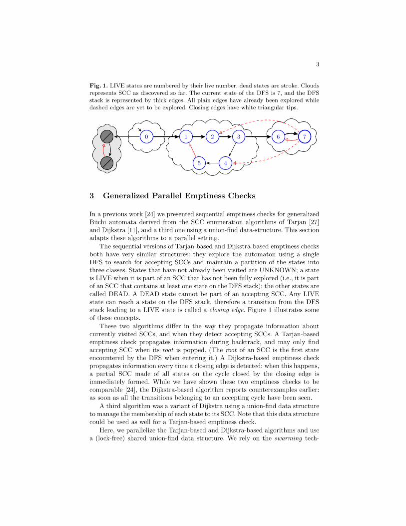
Fig. 1. LIVE states are numbered by their live number, dead states are stroke. Cloudsrepresents SCC as discovered so far. The current state of the DFS is 7, and the DFSstack is represented by thick edges. All plain edges have already been explored whiledashed edges are yet to be explored. Closing edges have white triangular tips.

0 1 2 3 6 7

5 4

3 Generalized Parallel Emptiness Checks

In a previous work [24] we presented sequential emptiness checks for generalizedBuchi automata derived from the SCC enumeration algorithms of Tarjan [27]and Dijkstra [11], and a third one using a union-find data-structure. This sectionadapts these algorithms to a parallel setting.

The sequential versions of Tarjan-based and Dijkstra-based emptiness checksboth have very similar structures: they explore the automaton using a singleDFS to search for accepting SCCs and maintain a partition of the states intothree classes. States that have not already been visited are UNKNOWN; a stateis LIVE when it is part of an SCC that has not been fully explored (i.e., it is partof an SCC that contains at least one state on the DFS stack); the other states arecalled DEAD. A DEAD state cannot be part of an accepting SCC. Any LIVEstate can reach a state on the DFS stack, therefore a transition from the DFSstack leading to a LIVE state is called a closing edge. Figure 1 illustrates someof these concepts.

These two algorithms differ in the way they propagate information aboutcurrently visited SCCs, and when they detect accepting SCCs. A Tarjan-basedemptiness check propagates information during backtrack, and may only findaccepting SCC when its root is popped. (The root of an SCC is the first stateencountered by the DFS when entering it.) A Dijkstra-based emptiness checkpropagates information every time a closing edge is detected: when this happens,a partial SCC made of all states on the cycle closed by the closing edge isimmediately formed. While we have shown these two emptiness checks to becomparable [24], the Dijkstra-based algorithm reports counterexamples earlier:as soon as all the transitions belonging to an accepting cycle have been seen.

A third algorithm was a variant of Dijkstra using a union-find data structureto manage the membership of each state to its SCC. Note that this data structurecould be used as well for a Tarjan-based emptiness check.

Here, we parallelize the Tarjan-based and Dijkstra-based algorithms and usea (lock-free) shared union-find data structure. We rely on the swarming tech-

4

Algorithm 1: Main procedure

1 Shared Variables:

2 A: TGBA of 〈Q, q0, δ,F〉3 stop: boolean

4 uf : union-find of 〈Q ∪ Dead , 2F 〉

5 Global Structures:

6 struct Step { src: Q, acc: 2F ,

7 pos: int , succ: 2δ }8 struct Transition {src: Q, acc: 2F

9 dst : Q}10 enum Strategy { Mixed, Tarjan,11 Dijkstra}12 enum Status { LIVE, DEAD,13 UNKNOWN}14 Local Variales:

15 dfs: stack of 〈Step〉16 live: stack of 〈Q 〉17 livenum: hashmap of 〈Q, int 〉18 pstack : stack of 〈P 〉

19 main(str : Strategy)20 stop ← ⊥21 uf .make set(〈Dead , ∅ 〉)22 if str 6= Mixed23 EC(str , 1) ‖ . . . ‖ EC(str , n)

24 else25 str ← Dijkstra26 EC(str , 1) ‖ . . . ‖ EC(str , bn

2c)

27 str ← Tarjan28 EC(str , 1+bn

2c) ‖ . . . ‖ EC(str , n)

29 Wait for all threads to finish

30 GET STATUS(q ∈ Q) → Status31 if livenum.contains(q)32 return LIVE

33 else if uf .contains(varq) ∧34 uf .same set(q , Dead)35 return DEAD

36 else37 return UNKNOWN

38 EC(str : Strategy , tid : int)39 seed(tid) // Random Number Gen.

40 PUSHstr(∅, q0)41 while ¬ dfs.empty() ∧ ¬ stop42 Step step ← dfs.top()43 if step.succ 6= ∅44 Transition t ← randomly45 pick one off from step.succ46 switch GET STATUS(t .dst)47 case DEAD48 skip

49 case LIVE50 UPDATEstr(t .acc, t .dst)

51 case UNKNOWN52 PUSHstr(t .acc, t .dst)

53 else54 POPstr(step)

55 stop ← >

nique: each thread execute the same algorithm, but explores the automaton ina different order [16]. Furthermore, threads will use the union-find to share in-formation about membership to SCCs, acceptance of these SCCs, and DEADstates. Note that the shared information is stable: the fact that two states belongto the same SCC, or that a state is DEAD will never change over the execu-tion of the algorithm. All threads may therefore reuse this information freely toaccelerate their exploration, and to find accepting cycles collaboratively.

5

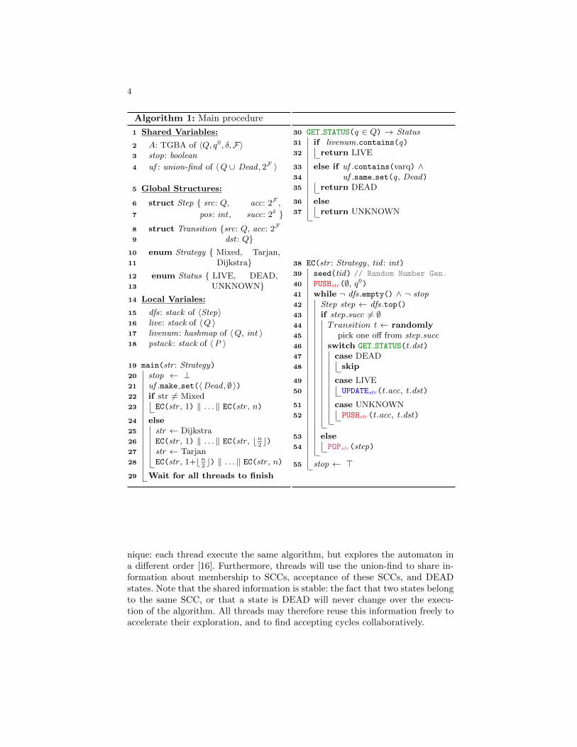
3.1 Generic Canvas

Algorithm 1 presents the structure common to the Tarjan-based and Dijkstra-based parallel emptiness checks.

All threads share the automaton A to explore, a stop variable used to stopall threads as soon an accepting cycle is found or one thread detects that thewhole automaton has been visited, and the union-find data-structure [20]. Theunion-find maintains the membership of each state to the various SCCs of theautomaton, or the set of DEAD states (a state is DEAD if it belongs to thesame class as the artificial Dead state). Furthermore this data structure hasbeen extended to store the acceptance marks occurring in an SCC.

The union-find structure partitions the set Q′ = Q∪{Dead} labeled with anelement of 2F and offers the following methods:

– make set(s ∈ Q′) creates a new class containing the state s if s is notalready in the union-find.

– contains(s ∈ Q′) checks whether s is already in the union-find.

– unite(s1 ∈ Q′, s2 ∈ Q′, acc ∈ 2F) merges the classes of s1 and s2, and addsthe acceptance marks acc to the resulting class. This method returns the setof acceptance marks of resulting class. However, when the class constructedby unite contains Dead , this method always returns ∅. An accepting cyclecan therefore be reported as soon as unite returns F .

– same set(s1 ∈ Q′, s2 ∈ Q′) checks whether two states are in the same class.

As suggested by Anderson and Woll [1], we implement a thread safe versionof this union-find structure using compare-and-swap since it relies on linked listsand an hash table.

The original sequential algorithms maintain a stack of LIVE states in orderto mark all states of an explored SCC as DEAD. In our previous work [24], wesuggested to use a union-find data structure for this, allowing to mark all statesof an SCC as dead by doing a single unite with an artificial Dead state. However,this notion of LIVE state (and closing edge detection) is obviously dependent onthe traversal order, and will therefore be different in each thread. Consequently,each thread has to keep track locally of its own LIVE states. Thus, each threadmaintains the following local variables:

– The dfs stack stores elements of type Step composed of the current state(src), the acceptance mark (acc) for the incoming transition (or ∅ for theinitial state), an identifier pos (whose use is different in Dijkstra and Tarjan)and the set succ of unvisited successors of the src state.

– The live stack stores all the LIVE states that are not on the dfs stack (assuggested by Nuutila and Soisalon-Soininen [19]).

– The hash map livenum associates each LIVE state to a (locally) uniqueincreasing identifier.

– pstack holds identifiers that are used differently in the emptiness checks ofthis paper.

6

With these data structures, a thread can decide whether a state is LIVE,DEAD, or UNKNOWN (i.e., new) by first checking livenum (a local structure),and then uf (a shared structure). This test is done by GET STATUS. Note thata state marked LIVE locally may have already been marked DEAD by anotherthread, thus leading to redundant work. However, avoiding this extra work wouldrequire more queries to the shared uf .

The procedure EC shows the generic DFS that will be executed by all threads.The order of the successors is chosen randomly in each thread, and the DFSstops as soon as one thread sets the stop flag. GET STATUS is called on eachreached state to decide how it has to be handled: DEAD states are ignored,UNKNOWN states are pushed on the dfs stack, and LIVE states correspond toclosing edges. This generic DFS is adapted to the Tarjan and Dijkstra strategiesby calling PUSHstr on new states, UPDATEstr on closing edges, and POPstr whenall the successors of a state have been visited by this thread.

Several parallel instances of this EC algorithm are instantiated by the main

procedure, possibly using different strategies. Each instance is parameterized bya unique identifier tid and a Strategy selecting either Dijkstra or Tarjan. If mainis called with the Mixed strategy, it instantiates a mix of both emptiness-checks.When one thread reports an accepting cycle or ends the exploration of the entireautomaton, it sets the stop variable, causing all threads to terminate. The main

procedure therefore only has to wait for all threads to terminate.

3.2 The Tarjan Strategy

Strategy 1 shows how the generic canvas is refined to implement the Tarjanstrategy. In this algorithm, each new LIVE state is numbered with the actualnumber of LIVE states during the PUSHTarjan operation. Furthermore each stateis associated to a lowlink, i.e., the smallest live number of any state known to bereachable from this state. These lowlinks, whose purpose is to detect the root ofeach SCC, are only maintained for the states on the dfs stack, and are stored onthe pstack .

These lowlinks are updated either when a closing edge is detected in theUPDATETarjan method (in this case the current state and the destination ofthe closing edge are in the same SCC) or when a non-root state is popped inPOPTarjan (in this case the current state and its predecessor on the dfs stack arein the same SCC). Every time a lowlink is updated, we therefore learn that twostates belong to the same SCC and can publish this fact to the shared uf tak-ing into account any acceptance mark between those two states. If the uf detectsthat the union of these acceptance marks with those already known for this SCCis F , then the existence of an accepting cycle can be reported immediately.

POPTarjan has two behaviors depending on whether the state being poppedis a root or not. At this point, a state is a root if its lowlink is equal to its livenumber. Non-root states are transferred from the dfs stack to the live stack.When a root state is popped, we first publish that all the SCC associated to thisroot is DEAD, and also locally we remove all these states from live and livenumusing the markdead function.

7

Strategy 1: Tarjan

struct P {p : int}

1 PUSHTarjan(acc ∈ 2F , q ∈ Q)2 uf .make set(q)3 p ← livenum.size()4 livenum.insert(〈 q , p 〉)5 pstack .push(〈 p 〉)6 dfs.push( 〈 q, acc, p, succ(q)〉 )7 UPDATETarjan(acc ∈ 2F , d ∈ Q)8 pstack .top().p ←9 min(pstack .top().p,

10 livenum.get(d))11 a ← uf .unite(d , dfs.top().src,12 acc)13 if a = F14 stop ← >15 report accepting cycle found

16 POPTarjan(s ∈ Step)17 dfs.pop()18 〈 ll 〉 ← pstack .pop()19 if ll = s.pos20 markdead(s)

21 else22 pstack .top().p ←23 min(pstack .top().p, ll)24 a ← uf .unite(s.src,25 dfs.top().src, s.acc)26 if a = F27 stop ← >28 report accepting cycle found

29 live.push(s.src)

Strategy 2: Dijkstra

struct P {p : int , acc : 2F}

1 PUSHDijkstra(acc ∈ 2F , q ∈ Q)2 uf .make set(q)3 p ← livenum.size()4 livenum.insert(〈 q , p 〉)5 pstack .push(〈dfs.size(), ∅ 〉)6 dfs.push( 〈 q, acc, p, succ(q)〉 )7 UPDATEDijkstra(acc ∈ 2F , d ∈ Q)8 dpos ← livenum.get(d)9 〈r ,a〉 ← pstack .top()

10 a ← a ∪ acc11 while dpos < dfs[r ].pos12 〈r , la〉 ← pstack .pop()13 a ← a ∪ dfs[r ].acc ∪ la14 a ← uf .unite(d , dfs[r ].src, a)

15 pstack .top().acc ← a16 if a = F17 stop ← >18 report accepting cycle found

19 POPDijkstra(s ∈ Step)20 dfs.pop()21 if pstack .top().p = dfs.size()22 pstack .pop()23 markdead(s)

24 else25 live.push(s.src)

26 // Common to all strategies.

27 markdead(s ∈ Step)28 uf .unite(s.src, Dead)29 livenum.remove(s.src)30 while livenum.size() > s.pos31 q ← live.pop()32 livenum.remove(q)

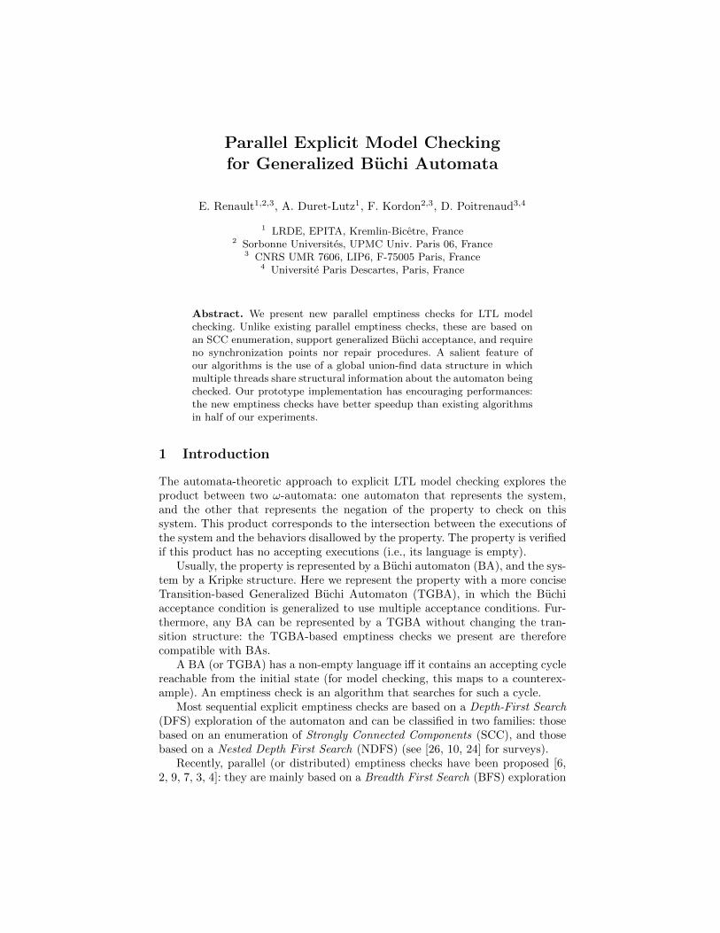
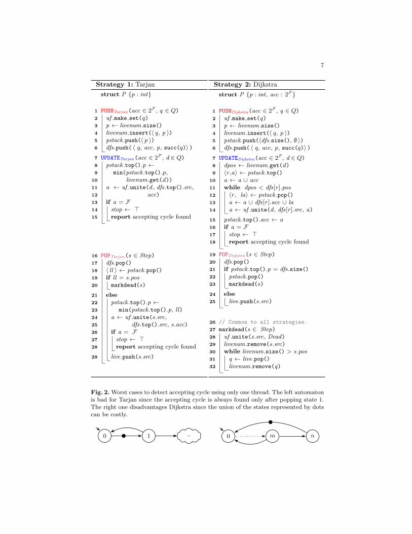
Fig. 2. Worst cases to detect accepting cycle using only one thread. The left automatonis bad for Tarjan since the accepting cycle is always found only after popping state 1.The right one disadvantages Dijkstra since the union of the states represented by dotscan be costly.

0 1 .. 0 m n

8

If there is no accepting cycle, the number of calls to unite performed in asingle thread by this strategy is always the number of transitions in each SCC(corresponding to the lowlink updates) plus the number of SCCs (correspondingto the calls to markdead). The next strategy performs fewer calls to unite.

3.3 The Dijkstra Strategy

Strategy 2 shows how the generic canvas is refined to implement the Dijkstrastrategy. The way LIVE states are numbered and the way states are marked asDEAD is identical to the previous strategy. The difference lies in the way SCCinformation is encoded and updated.

This algorithm maintains pstack , a stack of potential roots, represented (1)by their positions p in the dfs stack (so that we can later retrieve the incomingacceptance marks and the live number of the potential roots), and (2) the unionacc of all the acceptance marks seen in the cycles visited around the potentialroot.

Here pstack is updated only when a closing edge is detected, but not whenbacktracking a non-root as done in Tarjan. When a closing edge is detected, thelive number dpos of its destination can be used to pop all the potential roots onthis cycle (those whose live number are greater than dpos), and merge the setsof acceptance marks along the way: this happens in UPDATEDijkstra . Note thatthe dfs stack has to be addressable like an array during this operation.

As it is presented, UPDATEDijkstra calls unite only when a potential root isdiscovered not be a root (lines 10–14). In the particular case where a closingedge does not invalidate any potential root, no unite operation is performed;still, the acceptance marks on this closing edge are updated locally line 15. Forinstance in Figure 1, when the closing edge (7, 4) is explored, the root of theright-most SCC (containing state 7) will be popped (effectively merging the tworight-most SCCs in uf ) but when the closing edge (7, 2) is later explored no popwill occur because the two states now belong to the same SCC. This strategytherefore does not share all its acceptance information with other threads. Inthis strategy, the acceptance accumulated in pstack locally are enough to detectaccepting cycles. However the unite operation on line 14 will also return someacceptance marks discovered by other threads around this state: this additionalinformation is also accumulated in pstack to speedup the detection of acceptingcycles.

In this strategy, a given thread only calls unite to merge two disjoint setsof states belonging to the same SCC. Thus, the total number of unite neededto build an SCC of n states is necessarily equal to n − 1. This is better thanthe Tarjan-based version, but it also means we share less information betweenthreads.

3.4 The Mixed Strategy

Figure 2 presents two situations on which Dijkstra and Tarjan strategies canclearly be distinguished.

9

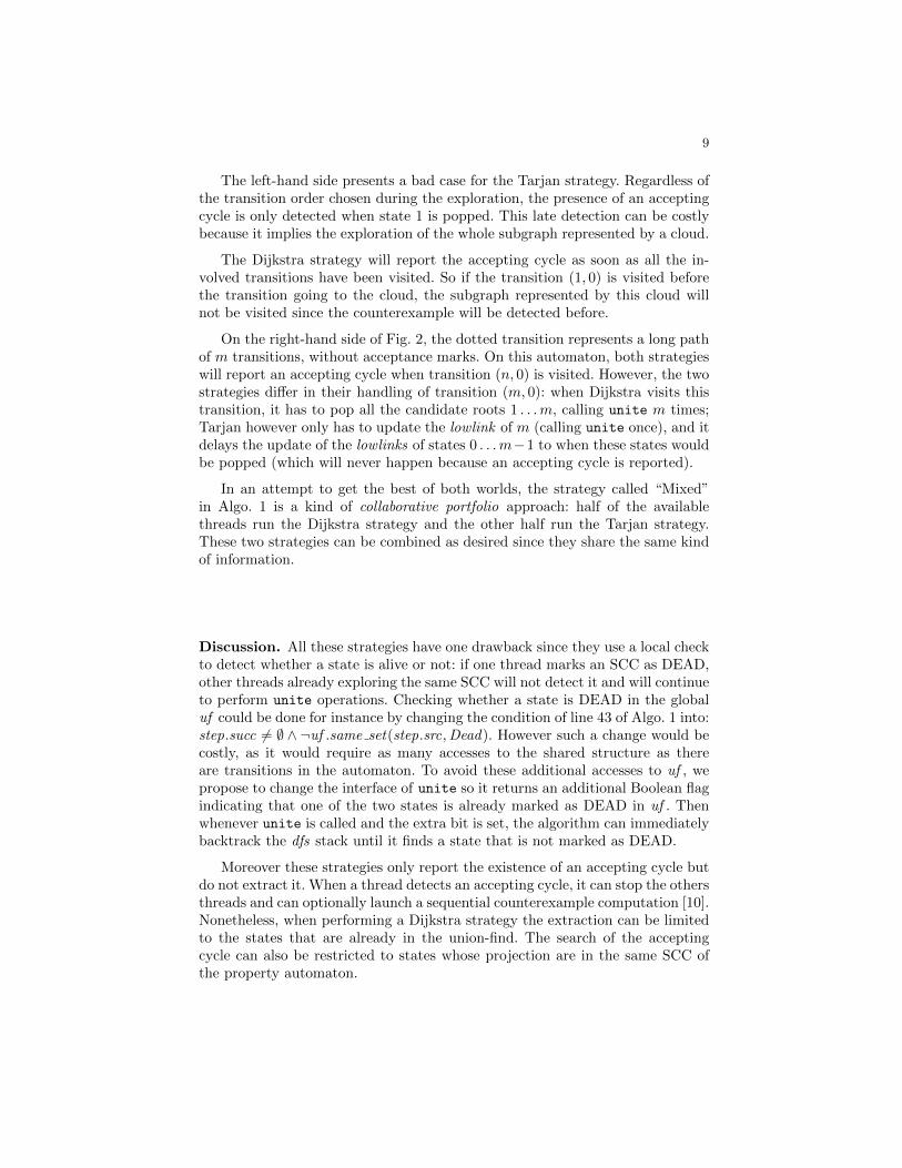
The left-hand side presents a bad case for the Tarjan strategy. Regardless ofthe transition order chosen during the exploration, the presence of an acceptingcycle is only detected when state 1 is popped. This late detection can be costlybecause it implies the exploration of the whole subgraph represented by a cloud.

The Dijkstra strategy will report the accepting cycle as soon as all the in-volved transitions have been visited. So if the transition (1, 0) is visited beforethe transition going to the cloud, the subgraph represented by this cloud willnot be visited since the counterexample will be detected before.

On the right-hand side of Fig. 2, the dotted transition represents a long pathof m transitions, without acceptance marks. On this automaton, both strategieswill report an accepting cycle when transition (n, 0) is visited. However, the twostrategies differ in their handling of transition (m, 0): when Dijkstra visits thistransition, it has to pop all the candidate roots 1 . . .m, calling unite m times;Tarjan however only has to update the lowlink of m (calling unite once), and itdelays the update of the lowlinks of states 0 . . .m−1 to when these states wouldbe popped (which will never happen because an accepting cycle is reported).

In an attempt to get the best of both worlds, the strategy called “Mixed”in Algo. 1 is a kind of collaborative portfolio approach: half of the availablethreads run the Dijkstra strategy and the other half run the Tarjan strategy.These two strategies can be combined as desired since they share the same kindof information.

Discussion. All these strategies have one drawback since they use a local checkto detect whether a state is alive or not: if one thread marks an SCC as DEAD,other threads already exploring the same SCC will not detect it and will continueto perform unite operations. Checking whether a state is DEAD in the globaluf could be done for instance by changing the condition of line 43 of Algo. 1 into:step.succ 6= ∅ ∧ ¬uf .same set(step.src,Dead). However such a change would becostly, as it would require as many accesses to the shared structure as thereare transitions in the automaton. To avoid these additional accesses to uf , wepropose to change the interface of unite so it returns an additional Boolean flagindicating that one of the two states is already marked as DEAD in uf . Thenwhenever unite is called and the extra bit is set, the algorithm can immediatelybacktrack the dfs stack until it finds a state that is not marked as DEAD.

Moreover these strategies only report the existence of an accepting cycle butdo not extract it. When a thread detects an accepting cycle, it can stop the othersthreads and can optionally launch a sequential counterexample computation [10].Nonetheless, when performing a Dijkstra strategy the extraction can be limitedto the states that are already in the union-find. The search of the acceptingcycle can also be restricted to states whose projection are in the same SCC ofthe property automaton.

10

3.5 Sketch of Proof

Due to lack of space, and since the Tarjan strategy is really close to the Dijkstrastrategy, we only give the scheme of a proof1 that the latter algorithm willterminate and will report a counterexample if and only if there is an acceptingcycle in the automaton.

Theorem 1. For all automata A the emptiness check terminates.

Theorem 2. The emptiness check reports an accepting cycle iff L (A) 6= ∅.

The theorem 1 is obvious since the emptiness check performs a DFS on afinite graph. Theorem 2 ensues from the invariants below which use the followingnotations. For any thread, n denotes the size of its pstack stack. For 0 ≤ i < n,Si denotes the set of states in the same partial SCC represented by pstack [i]:

Si =

{q ∈ livenum

∣∣∣∣∣ dfs[pstack [i].p].pos ≤ livenum[q]

livenum[q] ≤ dfs[pstack [i+ 1].p].pos

}for i < n− 1

Sn−1 = {q ∈ livenum | dfs[pstack [n− 1].p].pos ≤ livenum[q]}

The following invariants hold for all lines of algorithm 1:

Invariant 1. pstack contains a subset of positions in dfs, in increasing order.

Invariant 2. For all 0 ≤ i < n − 1, there is a transition with the acceptancemarks dfs[pstack [i+ 1].p].acc between Si and Si+1.

Invariant 3. For all 0 ≤ i < n, the subgraph induced by Si is a partial SCC.

Invariant 4. If the class of a state inside the union-find is associated to acc 6= ∅,then the SCC containing this state has a cycle visiting acc. (Note: a state in thesame class as Dead is always associated to ∅.)Invariant 5. The first thread marking a state as DEAD has seen the full SCCcontaining this state.

Invariant 6. The set of DEAD states is a union a maximal SCC.

Invariant 7. If a state is DEAD it cannot be part of an accepting cycle.

These invariants establish both directions of Theorem 2: invariants 1–4 provethat when the algorithm reports a counterexample there exists a cycle visiting allacceptance marks; invariants 5–7 justify that when the algorithm exits withoutreporting anything, then no state can be part of a counterexample.

4 Implementation and Benchmarks

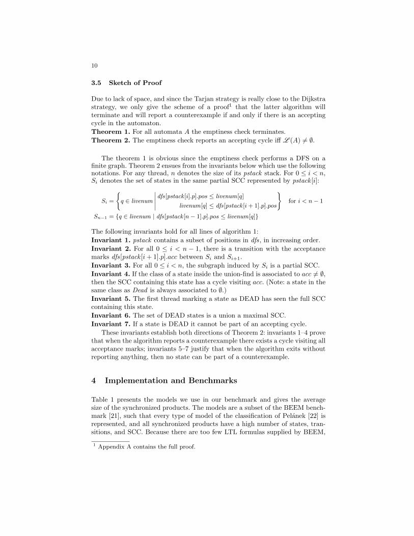
Table 1 presents the models we use in our benchmark and gives the averagesize of the synchronized products. The models are a subset of the BEEM bench-mark [21], such that every type of model of the classification of Pelanek [22] isrepresented, and all synchronized products have a high number of states, tran-sitions, and SCC. Because there are too few LTL formulas supplied by BEEM,

1 Appendix A contains the full proof.

11

Table 1. Statistics about synchronized products having an empty language (X) andnon-empty one (×).

Avg. States Avg. Trans. Avg. SCCsModel (X) (×) (X) (×) (X) (×)

adding.4 5 637 711 7 720 939 10 725 851 14 341 202 5 635 309 7 716 385bridge.3 1 702 938 3 114 566 4 740 247 8 615 971 1 701 048 3 106 797

brp.4 15 630 523 38 474 669 33 580 776 94 561 556 4 674 238 16 520 165collision.4 30 384 332 101 596 324 82 372 580 349 949 837 347 535 22 677 968

cyclic-sched 724 400 1 364 512 6 274 289 12 368 800 453 547 711 794elevator.4 2 371 413 3 270 061 7 001 559 9 817 617 1 327 005 1 502 808

elevator2.3 10 339 003 13 818 813 79 636 749 120 821 886 2 926 881 6 413 279exit.3 3 664 436 8 617 173 11 995 418 29 408 340 3 659 550 8 609 674

leader-el.3 546 145 762 684 3 200 607 4 033 362 546 145 762 684prod-cell.3 2 169 112 3 908 715 7 303 450 13 470 569 1 236 881 1 925 909

we opted to generate random formulas to verify on each model. We computed atotal number of 3268 formulas.2

The presented algorithms deal with any kind of generalized Buchi automata,but there exists specialized algorithms for subclasses of Buchi automata. Forinstance the verification of a safety property reduces to a reachability test. Sim-ilarly, persistent properties can be translated into automata where SCC can-not mix accepting cycles with non-accepting cycles [8] and for which a simpleremptiness check exists. Our benchmark contains only non-persistent properties,requiring a general emptiness check.

Among the 3268 formulas, 1706 result in products with the model havingan empty language (the emptiness check may terminate before exploring thefull product). All formulas were selected so that the sequential NDFS emptinesscheck of Gaiser and Schwoon [15] would take between 15 seconds and 30 minuteson an four Intel(R) Xeon(R) CPUX7460@ 2.66GHz with 128GB of RAM. This24-core machine is also used for the following parallel experiments.

All the approaches mentioned in Section 3 have been implemented in Spot [12].The union-find structure is lock-free and uses two common optimizations: “Im-mediate Parent Check”, and “Path Compression” [20].

The seed used to choose a successor randomly depends on the thread identifiertid passed to EC. Thus our strategies have the same exploration order whenexecuted sequentially; otherwise this order may be altered by information sharedby other threads.

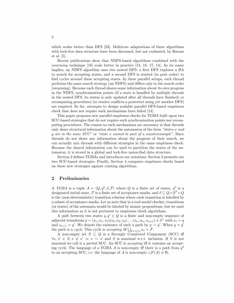
Figure 3 presents the comparison of our prototype implementation in Spotagainst the cndfs algorithm implemented in LTSmin and the owcty algorithmimplemented in DiVine 2.4. We selected owcty because it is reported to be the

2 For a description of our setup, including selected models, formulas, and detailedresults, see http://www.lrde.epita.fr/~renault/benchs/TACAS-2015/results.

html.

12

most efficient parallel emptiness check based on a non-DFS exploration, whilecndfs is reported to be the most efficient based on a DFS [14].

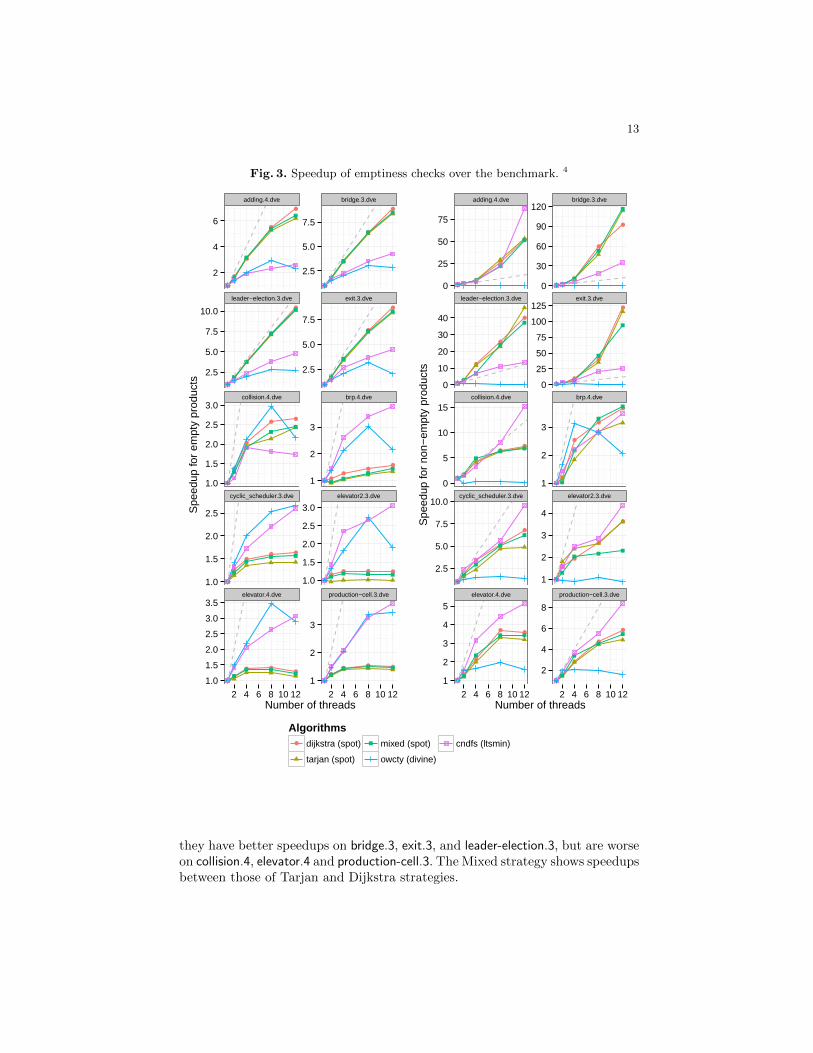
We generate the corresponding system automata using the version of DiVinE2.4 patched by the LTSmin team.3 For each emptiness check, we limit the ex-ecution time to one hour: all the algorithms presented in this paper proceessthe 3268 synchronized products within this limit while owcty fails over 11 casesand cndfs fails over 784 cases. DiVinE and LTSmin implement all sorts ofoptimizations (like state compression, caching of successors, dedicated memoryallocator...) while our implementation in Spot is still at a prototype stage. So inabsolute time, the sequential version of cndfs is around 3 time faster5 than ourprototype implementation which is competitive to DiVinE. Since the implemen-tations are different, we therefore compare the average speedup of the parallelversion of each algorithm against its sequential version. The actual time can befound in the detailed results2.

The left-hand side of Figure 3 shows those speedups, averaged for each model,for verified formulas (where the entire product has to be explored). First, itappears that the Tarjan strategy’s speedup is always lower than those of Dijkstraor Mixed for empty products. These low speedups can be explained by contentionon the shared union-find data structure during unite operations. In an SCC ofn states and m edges, a thread applying the Tarjan strategy performs m unite

calls while applying Dijkstra one needs only n−1 unite invocations before theyboth mark the whole SCC as DEAD with a unique unite call.

Second, for all strategies we can distinguish two groups of models. For adding.4,bridge.3, exit.3, and leader-election.3, the speedups are quasi-linear. However forthe other six models, the speedups are much more modest: it seems that addingnew threads quickly yield no benefits. A look to absolute time (for the first group)shows that the Dijkstra strategy is 25% faster than cndfs using 12 threads whereit was two time slower with only one thread.

A more detailed analysis reveals that products of the first group have manysmall SCC (organized in a tree shape) while products of the second group havea few big SCC. These big SCC have more closing edges: the union-find datastructure is stressed at every unite. This confirms what we observed for theTarjan strategy about the impact of unite operations.

The right-hand side of Figure 3 shows speedups for violated formulas. Inthese cases, the speedup can exceed the number of threads since the differentthreads explore the product in different orders, thus increasing the probability toreport an accepting cycle earlier. The three different strategies have comparablespeedup for all models, however their profiles differ from cndfs on some models:

3 http://fmt.cs.utwente.nl/tools/ltsmin/#divine4 This figure can be zoomed in color in the electronic version.5 Note that the time measured for cndfs does not includes the on-the-fly generation

of the product (it is precalculated because doing the on-the-fly product in LTSminexhibits a bug) while the time measured for the others includes the generation ofthe product.

13

Fig. 3. Speedup of emptiness checks over the benchmark. 4

●

●

●

●

●

●

●

●

●

●

●

●

●

●

●

●

●

●

●

●

●

●

●

●●

● ●●

●●

●

●

●● ●

●●

● ● ●

●●

● ●●

●●

● ● ●

adding.4.dve bridge.3.dve

leader−election.3.dve exit.3.dve

collision.4.dve brp.4.dve

cyclic_scheduler.3.dve elevator2.3.dve

elevator.4.dve production−cell.3.dve

2

4

6

2.5

5.0

7.5

2.5

5.0

7.5

10.0

2.5

5.0

7.5

1.0

1.5

2.0

2.5

3.0

1

2

3

1.0

1.5

2.0

2.5

1.0

1.5

2.0

2.5

3.0

1.0

1.5

2.0

2.5

3.0

3.5

1

2

3

2 4 6 8 10 12 2 4 6 8 10 12Number of threads

Spe

edup

for

empt

y pr

oduc

ts

● ●●

●

●

● ●●

●

●

●●

●

●

●

● ●●

●

●

●●

●

●●

●●

●

●

●

●

●

●

●

●

●

●

●

●

●

●●

●

● ●

●●

●

●

●

adding.4.dve bridge.3.dve

leader−election.3.dve exit.3.dve

collision.4.dve brp.4.dve

cyclic_scheduler.3.dve elevator2.3.dve

elevator.4.dve production−cell.3.dve

0

25

50

75

0

30

60

90

120

0

10

20

30

40

0

25

50

75

100

125

0

5

10

15

1

2

3

2.5

5.0

7.5

10.0

1

2

3

4

1

2

3

4

5

2

4

6

8

2 4 6 8 10 12 2 4 6 8 10 12Number of threads

Spe

edup

for

non−

empt

y pr

oduc

ts

Algorithms● dijkstra (spot)

tarjan (spot)

mixed (spot)

owcty (divine)

cndfs (ltsmin)

they have better speedups on bridge.3, exit.3, and leader-election.3, but are worseon collision.4, elevator.4 and production-cell.3. The Mixed strategy shows speedupsbetween those of Tarjan and Dijkstra strategies.

14

5 Conclusion

We have presented some first and new parallel emptiness checks based on anSCC enumeration. Our approach departs from state-of-the-art emptiness checkssince it is neither BFS-based nor NDFS-based. Instead it parallelizes SCC-basedemptiness checks that are built over a single DFS. Our approach supports gen-eralized Buchi acceptance, and requires no synchronization points nor repairprocedures. We therefore answer positively to the question raised by Evange-lista et al. [14]: “Is the design of a scalable linear-time algorithm without repairprocedures or synchronisation points feasible?”. Our prototype implementationhas encouraging performances: the new emptiness checks have better speedupthan existing algorithms in half of our experiments, making them suitable forportfolio approaches.

The core of our algorithms relies on a union-find (lock-free) data structure toshare structural information between multiple threads. The use of a union-findseems adapted to this problem, and yet it has never been used for parallel empti-ness checks (and only recently for sequential emptiness checks [24]): we believethat this first use might stimulate other researchers to derive new emptinesschecks or ideas from it.

In some future work, we would like to investigate different variations of ouralgorithms. For instance could the information shared in the union-find be usedto better direct the DFS performed by the Dijkstra or Tarjan strategies and helpto balance the exploration of the automaton by the various threads? We wouldalso like to implement Gabow’s algorithm that we presented in a sequentialcontext [24] in this same parallel setup. Changing the architecture, we wouldlike to explore how the union-find data structure could be adapted to developasynchronous algorithms where one thread could call unite without waiting foran answer. Another topic is to explore the use of SCC strengths [25] to improveparallel emptiness checks.

References

1. R. J. Anderson and H. Woll. Wait-free parallel algorithms for the union-findproblem. In Proc. 23rd ACM Symposium on Theory of Computing, pp. 370–380,1994.

2. J. Barnat, L. Brim, and J. Chaloupka. Parallel breadth-first search LTL model-checking. In ASE’03, pp. 106–115. IEEE Computer Society, 2003.

3. J. Barnat, L. Brim, and J. Chaloupka. From distributed memory cycle detection toparallel LTL model checking. In FMICS’04, vol. 133 of ENTCS, pp. 21–39, 2005.

4. J. Barnat, L. Brim, and P. Rockai. A time-optimal on-the-fly parallel algorithmfor model checking of weak LTL properties. In ICFEM’09, vol. 5885 of LNCS, pp.407–425, 2009. Springer.

5. J. Barnat, L. Brim, and P. Rockai. Scalable shared memory LTL model checking.STTT, 12(2):139–153, 2010.

6. L. Brim, I. Cerna, P. Krcal, and R. Pelanek. Distributed LTL model checkingbased on negative cycle detection. In FSTTCS’01, pp. 96–107, 2001.

15

7. L. Brim, I. Cerna, P. Moravec, and J. Simsa. Accepting predecessors are betterthan back edges in distributed LTL model-checking. In FMCAD’04, vol. 3312 ofLNCS, pp. 352–366. Springer, November 2004.

8. I. Cerna and R. Pelanek. Relating hierarchy of temporal properties to modelchecking. In MFCS’03, vol. 2747 of LNCS, pp. 318–327, Aug. 2003. Springer.

9. I. Cerna and R. Pelanek. Distributed explicit fair cycle detection (set based ap-proach). In SPIN’03, vol. 2648 of LNCS, pp. 49–73. Springer, May 2003.

10. J.-M. Couvreur, A. Duret-Lutz, and D. Poitrenaud. On-the-fly emptiness checksfor generalized Buchi automata. In SPIN’05, vol. 3639 of LNCS, pp. 143–158.Springer, Aug. 2005.

11. E. W. Dijkstra. EWD 376: Finding the maximum strong components in a directedgraph. http://www.cs.utexas.edu/users/EWD/ewd03xx/EWD376.PDF, May 1973.

12. A. Duret-Lutz and D. Poitrenaud. SPOT: an Extensible Model Checking Libraryusing Transition-based Generalized Buchi Automata. In MASCOTS’04, pp. 76–83,Oct. 2004. IEEE Computer Society Press.

13. S. Evangelista, L. Petrucci, and S. Youcef. Parallel nested depth-first searches forLTL model checking. In ATVA’11, vol. 6996 of LNCS, pp. 381–396. Springer, 2011.

14. S. Evangelista, A. Laarman, L. Petrucci, and J. van de Pol. Improved multi-corenested depth-first search. In ATVA’12, vol. 7561 of LNCS, pp. 269–283. Springer,2012.

15. A. Gaiser and S. Schwoon. Comparison of algorithms for checking emptiness onBuchi automata. In MEMICS’09, vol. 13 of OASICS. Schloss Dagstuhl, Leibniz-Zentrum fuer Informatik, Germany, Nov. 2009.

16. G. J. Holzmann, R. Joshi, and A. Groce. Swarm verification techniques. IEEETransaction on Software Engineering, 37(6):845–857, 2011.

17. A. Laarman and J. van de Pol. Variations on multi-core nested depth-first search.In PDMC, pp. 13–28, 2011.

18. A. Laarman, R. Langerak, J. van de Pol, M. Weber, and A. Wijs. Multi-core nesteddepth-first search. In ATVA’11, vol. 6996 of LNCS, pp. 321–335, October 2011.Springer.

19. E. Nuutila and E. Soisalon-Soininen. On finding the strongly connected compo-nents in a directed graph. Information Processing Letters, 49(1):9–14, Jan. 1994.

20. M. M. A. Patwary, J. R. S. Blair, and F. Manne. Experiments on union-findalgorithms for the disjoint-set data structure. In SEA’10, vol. 6049 of LNCS, pp.411–423. Springer, 2010.

21. R. Pelanek. BEEM: benchmarks for explicit model checkers. In SPIN’07, vol. 4595of LNCS, pp. 263–267. Springer, 2007.

22. R. Pelanek. Properties of state spaces and their applications. International Journalon Software Tools for Technology Transfer (STTT), 10:443–454, 2008.

23. J. H. Reif. Depth-first search is inherently sequential. Information ProcessingLetters, 20:229–234, 1985.

24. E. Renault, A. Duret-Lutz, F. Kordon, and D. Poitrenaud. Three SCC-basedemptiness checks for generalized Buchi automata. In LPAR’13, vol. 8312 of LNCS,pp. 668–682. Springer, Dec. 2013.

25. E. Renault, A. Duret-Lutz, F. Kordon, and D. Poitrenaud. Strength-based decom-position of the property buchi automaton for faster model checking. In TACAS’13,vol. 7795 of LNCS, pp. 580–593. Springer, 2013.

26. S. Schwoon and J. Esparza. A note on on-the-fly verification algorithms. InTACAS’05, vol. 3440 of LNCS, Apr. 2005. Springer.

27. R. Tarjan. Depth-first search and linear graph algorithms. SIAM Journal onComputing, 1(2):146–160, 1972.

16

This appendix is for interested reviewers and not meant for publication.

A Sketch of Proof for the Dijkstra-based EmptinessCheck

To prove the Dijkstra strategy we assume that each line of algorithm 1 andstrategy 2 is executed atomically. This hypothesis is realistic because (1) theunion-find we use is lock-free, and (2) the only other shared variable is the stopvariable that can also be modified using compare-and-swap instructions.

We only provide a proof of Theorem 2, since Theorem 1 is the consequenceof doing a DFS.Theorem 2. The emptiness check reports an accepting cycle iff L (A) 6= ∅.

The proof uses following definitions and notations:

- A state is locally alive iff it is present in the local hashmap livenum of athread;

- A state is dead iff it is present in the shared union-find structure (uf ) and ifit is in the same partition than the artificial state Dead ;

- For any thread, n denotes the size of its pstack stack.- For 0 ≤ i < n, Si denotes the set of states in the same partial SCC repre-

sented by pstack [i], i.e.:

Si =

{q ∈ livenum

∣∣∣∣∣ dfs[pstack [i].p].pos ≤ livenum[q]

livenum[q] ≤ dfs[pstack [i+ 1].p].pos

}for i < n− 1

Sn−1 = {q ∈ livenum | dfs[pstack [n− 1].p].pos ≤ livenum[q]}

Some of these definitions and notations are represented Figure 4. In thefollowing, we prove each invariant independently. Then all these invariants areused to prove the one theorem.

Invariant 1. pstack contains a subset of positions in dfs, in increasing order.

Proof. By definition pstack holds positions of elements inside the dfs stack. Sowe only have to prove that they are increasing. During a PUSHDijkstra operation,dfs and pstack are both enlarged and the new value pushed on the top pstack(dfs.size()) is necessarily greater than the others values of pstack (strategy 2,line 5).

Moreover, the size of pstack is only decreased during a POPDijkstra (strategy 2,line 22) and during an UPDATEDijkstra (strategy 2, line 12). UPDATEDijkstra removeselements from pstack without removing elements from dfs, so the invariant stillholds. POPDijkstra removes element from dfs, but any such element of pstack isalso removed. �

Invariant 2. For all 0 ≤ i < n−1, there is a transition with the acceptance marksdfs[pstack [i+1].p].acc between Si and Si+1. More precisely: for all 0 ≤ i < n−1,there exists ` ∈ 2AP , such that (dfs[pos − 1].src, `, dfs[pos].acc, dfs[pos].src) ∈∆, with pos = pstack [i+ 1].p

17

Proof. After the first call to PUSHDijkstra (algorithm 1, line 39), the initial stateis inserted in the stacks dfs and pstack (strategy 2, line 5–6). Then n = 1 and theinvariant is trivially verified. Variables pstack and dfs are also modified duringPUSHDijkstra operations (algorithm 1, line 51). The new position inserted in pstack(strategy 2, line 5) references the state inserted in dfs (strategy 2, line 6). Bydefinition and since n has just been increased, the state dfs[pstack [i+1].p−1].srcwith i = n− 2, represents the top of the stack dfs before the call to PUSHDijkstra .This state is the source of the transition computed line 43 (algorithm 1). Beforeline 51 (algorithm 1), pstack [n− 1].p references the top element of the dfs stack.After line 51 (algorithm 1), dfs[pstack [n − 1].p].src is the destination of thetransition computed line 43 while dfs[pstack [n − 1].p].acc is the acceptance setof this transition. Invariant 2 is therefore preserved by PUSHDijkstra .

UPDATEDijkstra and a POPDijkstra can only modify pstack by doing some callsto pop but decreasing n preserves the invariant (strategy 2, line 12 and 22).Furthermore, invariant 1 ensures that pstack is a subset of positions in dfs. �

Invariant 3. For all 0 ≤ i < n, the subgraph induced by Si is a partial SCC.

Proof. Here again, we only focus on lines impacting the pstack variable. Afterthe first call to PUSHDijkstra , the initial state is in the dfs stack and the onlyelement in the stack pstack references this (initial) state. Therefore the invariantis trivially verified. In the same way, after every call to PUSHDijkstra (strategy ??,line 51) a partial SCC composed of a unique state is created. The invariant isthen trivially verified.

dfs

live

dead states

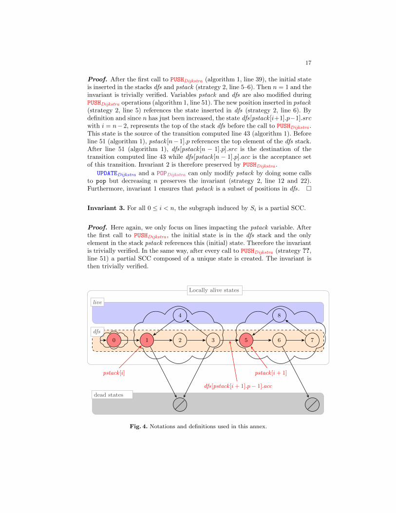
Locally alive states

0 1 2 3 5 6 7

4 8

pstack [i] pstack [i+ 1]

dfs[pstack [i+ 1].p− 1].acc

Fig. 4. Notations and definitions used in this annex.

18

When a closing edge is detected UPDATEDijkstra is called (algorithm 1, line 49).At this moment the destination of the closing edge d belongs to some partialSCC Sj . If Sj is the top partial SCC (j = n − 1) the size of pstack is notmodified (the while loop is not entered at line 11 of strategy 2) and the invariantis preserved. If j is smaller than n − 1, thanks to the invariants 2–3, there is apath between Sj and Sn−1 and because of the considered closing edge there isalso a path between Sj and Sn−1. As a consequence, Sj ∪ . . . ∪ Sn−1 forms apartial SCC. After the execution of the while loop, pstack has been popped sothat it size equals j + 1, and the new Sj contains all the states of the previousunion. �

Invariant 4. If the class of a state inside the union-find is associated to acc 6= ∅,then the SCC containing this state has a cycle visiting acc. (Note: a state in thesame class as Dead is always associated to ∅.)

Proof. By definition, the first call to make set(s), with s ∈ Q, associates s to∅ in the shared union-find (strategy 2, line 2). In the same way, all states in thesame partition than the artificial state Dead are associated to ∅ (strategy 2, line28). In the two previous situations the invariant is trivially verified.

The acceptance set is only modified at line 15 (strategy 2). In this case,the new acceptance set results from previous unite operations (strategy 2, line14). According to invariant 3, we know that the acceptance set passed to unite

represents (a part of) acceptance set in the current SCC. For line 14 (strategy 2)we distinguish only three cases because, by definition, unite returns either ∅ ora superset of the acceptance set given in parameter:

– the acceptance set returned by unite is ∅, the invariant is verified.– the acceptance set returned by unite is equal to the parameter a. The in-

variant is verified.– the acceptance set returned is a superset of the parameter a. The other

acceptance marks can only come from a unite operation of other thread(strategy 2, line 14). In this case we know that there exists a cycle visitingthese acceptance marks (invariant 3). The union of acceptance marks is thenvalid.

�

Invariant 5. The first thread marking a state as DEAD has seen the full SCCcontaining this state.

Proof. A state is marked DEAD only during the markdead operation (preciselyline 28 of strategy 2). A thread can call this method only if it detects that thetop of pstack is equal to the dfs size (the root for the partial SCC represented bySi). During the unite operation with the artificial state Dead , this thread hasseen all states of Si (which is a partial SCC according to invariant 3) and all non-DEAD states (according to lines 30 to 37 of algorithm 1). Then we distinguishtwo cases:

19

- this thread is the first marking DEAD a state of this SCC. Then Si containsall states of this SCC. Indeed, if Si does not contains all states of the SCC,there is a state which has not been visited. Since only DEAD states areignored, it means that another thread marked this state as DEAD: thiscontradicts the fact that the thread is the first marking dead a state of thisSCC.

– otherwise it’s not the first thread.

�

Invariant 6. The set of DEAD states is a union of maximal SCC.

Proof. When the first thread marks a state x as DEAD, it has seen all statesand transitions of this SCC (invariant 5). Therefore it has seen all the closingedges. Since there is at least one closing edge per cycle and each closing edgecauses the entire cycle to be united by UPDATEDijkstra , all the states of all thecycles have been merged into a single class that contains x. The call to markdead

by this first thread will therefore add a maximal SCC to the DEAD states.When any later thread marks a state as DEAD, the resulting call to unite

has no effect since all the states of this SCC have already been marked DEADby the first thread. �

Invariant 7. If a state is DEAD, it cannot be part of an accepting cycle.

Proof. According to invariant 5, the first thread marking an SCC as dead hasvisited the whole SCC. During this exploration, all the states of all the cycles ofthe SCC have been merged in a single class (strategy 2, line 14) and the union-find has accumulated all the acceptance sets of the all the transitions of theSCC. When a state is about to be marked as DEAD for the first time (strategy2, line 23), we know two things: (1) the entire SCC has been merged into a singleclass (proof of invariant 6), and (2) the union-find has accumulated the unionX of all acceptance marks of the SCC. We necessarily have X 6= 2F otherwise acounterexample would have been reported on line 16 (strategy 2). Consequentlythis SCC cannot contain an accepting cycle. �

Proof of theorem 2. (=⇒) The counterexample detection can only happen atline 16 of strategy 2. This detection depends of the acceptance set at the top ofthe stack pstack (strategy 2, lines 15–16). From invariants 1 to 4 we know thatthere exists a cycle that visits all these acceptance marks. (⇐=) Let us assumethat the algorithm terminates without reporting a counterexample. Consider thefirst thread that reaches line 54: it necessarily exited the while loop because dfswas empty. Thus, this thread has marked as DEAD all descendants of the initialstate that were not already marked DEAD by another thread. As a consequence,no state of the automaton can be part of a counterexample. �