CIMA Paper P1

Management Accounting

Study Text

Published by: Kaplan Publishing UK

Unit 2 The Business Centre, Molly Millars Lane, Wokingham, Berkshire RG41 2QZ

Copyright © 2015 Kaplan Financial Limited. All rights reserved.

No part of this publication may be reproduced, stored in a retrieval system or transmitted in any form or by any means electronic, mechanical, photocopying, recording or otherwise without the prior written permission of the publisher.

Acknowledgements

We are grateful to the CIMA for permission to reproduce past examination questions. The answers to CIMA Exams have been prepared by Kaplan Publishing, except in the case of the CIMA November 2010 and subsequent CIMA Exam answers where the official CIMA answers have been reproduced.

Notice

The text in this material and any others made available by any Kaplan Group company does not amount to advice on a particular matter and should not be taken as such. No reliance should be placed on the content as the basis for any investment or other decision or in connection with any advice given to third parties. Please consult your appropriate professional adviser as necessary. Kaplan Publishing Limited and all other Kaplan group companies expressly disclaim all liability to any person in respect of any losses or other claims, whether direct, indirect, incidental, consequential or otherwise arising in relation to the use of such materials.

Kaplan is not responsible for the content of external websites. The inclusion of a link to a third party website in this text should not be taken as an endorsement.

British Library Cataloguing in Publication Data

A catalogue record for this book is available from the British Library.

ISBN: 978­1­78415­299­4

Printed and bound in Great Britain.

ii

Contents

Page

Chapter 1 Traditional costing 1

Chapter 2 Activity­based costing 47

Chapter 3 Other costing techniques 81

Chapter 4 The modern manufacturing environment and the importance of quality

127

Chapter 5 Break­even analysis 167

Chapter 6 Relevant costs and decision making 223

Chapter 7 Linear programming 275

Chapter 8 Variance analysis: calculations 307

Chapter 9 Variance analysis: discussion elements 393

Chapter 10 Advanced variances 415

Chapter 11 The budgeting framework 481

Chapter 12 Budgetary control 535

Chapter 13 Forecasting techniques 575

Chapter 14 The treatment of uncertainty and risk in decision making

615

iii

iv

Introduction

v

chapterIntro

How to use the materials

These official CIMA learning materials have been carefully designed to make your learning experience as easy as possible and to give you the best chances of success in your Objective Test Examination.

The product range contains a number of features to help you in the study process. They include:

This Study Text has been designed with the needs of home study and distance learning candidates in mind. Such students require very full coverage of the syllabus topics, and also the facility to undertake extensive question practice. However, the Study Text is also ideal for fully taught courses.

The main body of the text is divided into a number of chapters, each of which is organised on the following pattern:

• a detailed explanation of all syllabus areas

• extensive ‘practical’ materials

• generous question practice, together with full solutions.

• Detailed learning outcomes. These describe the knowledge expected after your studies of the chapter are complete. You should assimilate these before beginning detailed work on the chapter, so that you can appreciate where your studies are leading.

• Step­by­step topic coverage. This is the heart of each chapter, containing detailed explanatory text supported where appropriate by worked examples and exercises. You should work carefully through this section, ensuring that you understand the material being explained and can tackle the examples and exercises successfully. Remember that in many cases knowledge is cumulative: if you fail to digest earlier material thoroughly, you may struggle to understand later chapters.

• Activities. Some chapters are illustrated by more practical elements, such as comments and questions designed to stimulate discussion.

vivi

If you work conscientiously through this Official CIMA Study Text according to the guidelines above you will be giving yourself an excellent chance of success in your Objective Test Examination. Good luck with your studies!

Quality and accuracy are of the utmost importance to us so if you spot an error in any of our products, please send an email to mykaplanreporting@kaplan.com with full details, or follow the link to the feedback form in MyKaplan.

Our Quality Co­ordinator will work with our technical team to verify the error and take action to ensure it is corrected in future editions.

• Question practice. The text contains three styles of question: – Exam­style objective test questions (OTQs)

– ‘Integration’ questions – these test your ability to understand topics within a wider context. This is particularly important with calculations where OTQs may focus on just one element but an integration question tackles the full calculation, just as you would be expected to do in the workplace.

– ‘Case’ style questions – these test your ability to analyse and discuss issues in greater depth, particularly focusing on scenarios that are less clear cut than in the Objective Test Examination, and thus provide excellent practice for developing the skills needed for success in the Operational Level Case Study Examination.

• Solutions. Avoid the temptation merely to ‘audit’ the solutions provided. It is an illusion to think that this provides the same benefits as you would gain from a serious attempt of your own. However, if you are struggling to get started on a question you should read the introductory guidance provided at the beginning of the solution, where provided, and then make your own attempt before referring back to the full solution.

Icon Explanations

Definition – These sections explain important areas of knowledge which must be understood and reproduced in an assessment environment.

Key point – Identifies topics which are key to success and are often examined.

Supplementary reading – These sections will help to provide a deeper understanding of core areas. The supplementary reading is NOT optional reading. It is vital to provide you with the breadth of knowledge you will need to address the wide range of topics within your syllabus that could feature in an assessment question. Reference to this text is vital when self studying.

Test your understanding – Following key points and definitions are exercises which give the opportunity to assess the understanding of these core areas.

vii

Illustration – To help develop an understanding of particular topics. The illustrative examples are useful in preparing for the Test your understanding exercises.

Exclamation mark – This symbol signifies a topic which can be more difficult to understand. When reviewing these areas, care should be taken.

Study technique

Passing exams is partly a matter of intellectual ability, but however accomplished you are in that respect you can improve your chances significantly by the use of appropriate study and revision techniques. In this section we briefly outline some tips for effective study during the earlier stages of your approach to the Objective Test Examination. We also mention some techniques that you will find useful at the revision stage.

Planning

To begin with, formal planning is essential to get the best return from the time you spend studying. Estimate how much time in total you are going to need for each subject you are studying. Remember that you need to allow time for revision as well as for initial study of the material.

With your study material before you, decide which chapters you are going to study in each week, and which weeks you will devote to revision and final question practice.

Prepare a written schedule summarising the above and stick to it!

It is essential to know your syllabus. As your studies progress you will become more familiar with how long it takes to cover topics in sufficient depth. Your timetable may need to be adapted to allocate enough time for the whole syllabus.

Students are advised to refer to the notice of examinable legislation published regularly in CIMA’s magazine (Financial Management), the students e­newsletter (Velocity) and on the CIMA website, to ensure they are up­to­date.

The amount of space allocated to a topic in the Study Text is not a very good guide as to how long it will take you. The syllabus weighting is the better guide as to how long you should spend on a syllabus topic.

Tips for effective studying

(1) Aim to find a quiet and undisturbed location for your study, and plan as far as possible to use the same period of time each day. Getting into a routine helps to avoid wasting time. Make sure that you have all the materials you need before you begin so as to minimise interruptions.

viii

(2) Store all your materials in one place, so that you do not waste time searching for items every time you want to begin studying. If you have to pack everything away after each study period, keep your study materials in a box, or even a suitcase, which will not be disturbed until the next time.

(3) Limit distractions. To make the most effective use of your study periods you should be able to apply total concentration, so turn off all entertainment equipment, set your phones to message mode, and put up your ‘do not disturb’ sign.

(4) Your timetable will tell you which topic to study. However, before diving in and becoming engrossed in the finer points, make sure you have an overall picture of all the areas that need to be covered by the end of that session. After an hour, allow yourself a short break and move away from your Study Text. With experience, you will learn to assess the pace you need to work at. Each study session should focus on component learning outcomes – the basis for all questions.

(5) Work carefully through a chapter, making notes as you go. When you have covered a suitable amount of material, vary the pattern by attempting a practice question. When you have finished your attempt, make notes of any mistakes you made, or any areas that you failed to cover or covered more briefly. Be aware that all component learning outcomes will be tested in each examination.

(6) Make notes as you study, and discover the techniques that work best for you. Your notes may be in the form of lists, bullet points, diagrams, summaries, ‘mind maps’, or the written word, but remember that you will need to refer back to them at a later date, so they must be intelligible. If you are on a taught course, make sure you highlight any issues you would like to follow up with your lecturer.

(7) Organise your notes. Make sure that all your notes, calculations etc. can be effectively filed and easily retrieved later.

Objective Test

Objective Test questions require you to choose or provide a response to a question whose correct answer is predetermined.

The most common types of Objective Test question you will see are:

• Multiple choice, where you have to choose the correct answer(s) from a list of possible answers. This could either be numbers or text.

• Multiple choice with more choices and answers, for example, choosing two correct answers from a list of eight possible answers. This could either be numbers or text.

• Single numeric entry, where you give your numeric answer, for example, profit is $10,000.

• Multiple entry, where you give several numeric answers.

ix

In every chapter of this Study Text we have introduced these types of questions, but obviously we have had to label answers A, B, C etc rather than using click boxes. For convenience we have retained quite a few questions where an initial scenario leads to a number of sub­questions. There will be questions of this type in the Objective Test Examination but they will rarely have more than three sub­questions.

Guidance re CIMA on­screen calculator

As part of the CIMA Objective Test software, candidates are now provided with a calculator. This calculator is on­screen and is available for the duration of the assessment. The calculator is available in each of the Objective Test Examinations and is accessed by clicking the calculator button in the top left hand corner of the screen at any time during the assessment.

All candidates must complete a 15­minute tutorial before the assessment begins and will have the opportunity to familiarise themselves with the calculator and practise using it.

Candidates may practise using the calculator by downloading and installing the practice exam at www.pearsonvue.com/cima/practiceexams/.

Fundamentals of Objective Tests

The Objective Tests are 90­minute assessments comprising 60 compulsory questions, with one or more parts. There will be no choice and all questions should be attempted.

• True/false questions, where you state whether a statement is true or false.

• Matching pairs of text, for example, matching a technical term with the correct definition.

• Other types could be matching text with graphs and labelling graphs/diagrams.

Structure of subjects and learning outcomes

Each subject within the syllabus is divided into a number of broad syllabus topics. The topics contain one or more lead learning outcomes, related component learning outcomes and indicative knowledge content.

A learning outcome has two main purposes:

(a) To define the skill or ability that a well prepared candidate should be able to exhibit in the examination.

(b) To demonstrate the approach likely to be taken in examination questions.

x

The learning outcomes are part of a hierarchy of learning objectives. The verbs used at the beginning of each learning outcome relate to a specific learning objective, e.g.

Calculate the break­even point, profit target, margin of safety and profit/volume ratio for a single product or service.

The verb ‘calculate’ indicates a level three learning objective. The following tables list the verbs that appear in the syllabus learning outcomes and examination questions.

CIMA VERB HIERARCHY

CIMA place great importance on the definition of verbs in structuring Objective Test Examinations. It is therefore crucial that you understand the verbs in order to appreciate the depth and breadth of a topic and the level of skill required. The Objective Tests will focus on levels one, two and three of the CIMA hierarchy of verbs. However they will also test levels four and five, especially at the management and strategic levels. You can therefore expect to be tested on knowledge, comprehension, application, analysis and evaluation in these examinations.

Level 1: KNOWLEDGE

What you are expected to know.

For example you could be asked to make a list of the advantages of a particular information system by selecting all options that apply from a given set of possibilities. Or you could be required to define relationship marketing by selecting the most appropriate option from a list.

VERBS USED

DEFINITION

List Make a list of.

State Express, fully or clearly, the details of/facts of.

Define Give the exact meaning of.

xi

Level 2: COMPREHENSION

What you are expected to understand.

For example you may be asked to distinguish between different aspects of the global business environment by dragging external factors and dropping into a PEST analysis.

Level 3: APPLICATION

How you are expected to apply your knowledge.

For example you may need to calculate the projected revenue or costs for a given set of circumstances.

VERBS USED

DEFINITION

Describe Communicate the key features of.

Distinguish Highlight the differences between.

Explain Make clear or intelligible/state the meaning or purpose of.

Identify Recognise, establish or select after consideration.

Illustrate Use an example to describe or explain something.

VERBS USED

DEFINITION

Apply Put to practical use.

Calculate Ascertain or reckon mathematically.

Demonstrate Prove with certainty or exhibit by practical means.

Prepare Make or get ready for use.

Reconcile Make or prove consistent/compatible.

Solve Find an answer to.

Tabulate Arrange in a table.

xii

Level 4: ANALYSIS

How you are expected to analyse the detail of what you have learned.

For example you may be required to interpret an inventory ratio by selecting the most appropriate statement for a given set of circumstances and data.

Level 5: EVALUATION

How you are expected to use your learning to evaluate, make decisions or recommendations.

For example you may be asked to recommend and select an appropriate course of action based on a short scenario.

VERBS USED

DEFINITION

Analyse Examine in detail the structure of.

Categorise Place into a defined class or division.

Compare/ contrast Show the similarities and/or differences between.

Construct Build up or compile.

Discuss Examine in detail by argument.

Interpret Translate into intelligible or familiar terms.

Prioritise Place in order of priority or sequence for action.

Produce Create or bring into existence.

VERBS USED

DEFINITION

Advise Counsel, inform or notify.

Evaluate Appraise or assess the value of.

Recommend Propose a course of action.

xiii

xiv

PRESENT VALUE TABLE

Present value of 1.00 unit of currency, that is ( ) nr −+1 where r = interest rate; n = number of periods until payment or receipt. Periods

(n) Interest rates (r)

1% 2% 3% 4% 5% 6% 7% 8% 9% 10% 1 0.990 0.980 0.971 0.962 0.952 0.943 0.935 0.926 0.917 0.909 2 0.980 0.961 0.943 0.925 0.907 0.890 0.873 0.857 0.842 0.826 3 0.971 0.942 0.915 0.889 0.864 0.840 0.816 0.794 0.772 0.751 4 0.961 0.924 0.888 0.855 0.823 0.792 0.763 0.735 0.708 0.683 5 0.951 0.906 0.863 0.822 0.784 0.747 0.713 0.681 0.650 0.621 6 0.942 0.888 0.837 0.790 0.746 0.705 0.666 0.630 0.596 0.564 7 0.933 0.871 0.813 0.760 0.711 0.665 0.623 0.583 0.547 0.513 8 0.923 0.853 0.789 0.731 0.677 0.627 0.582 0.540 0.502 0.467 9 0.914 0.837 0.766 0.703 0.645 0.592 0.544 0.500 0.460 0.424 10 0.905 0.820 0.744 0.676 0.614 0.558 0.508 0.463 0.422 0.386 11 0.896 0.804 0.722 0.650 0.585 0.527 0.475 0.429 0.388 0.350 12 0.887 0.788 0.701 0.625 0.557 0.497 0.444 0.397 0.356 0.319 13 0.879 0.773 0.681 0.601 0.530 0.469 0.415 0.368 0.326 0.290 14 0.870 0.758 0.661 0.577 0.505 0.442 0.388 0.340 0.299 0.263 15 0.861 0.743 0.642 0.555 0.481 0.417 0.362 0.315 0.275 0.239 16 0.853 0.728 0.623 0.534 0.458 0.394 0.339 0.292 0.252 0.218 17 0.844 0.714 0.605 0.513 0.436 0.371 0.317 0.270 0.231 0.198 18 0.836 0.700 0.587 0.494 0.416 0.350 0.296 0.250 0.212 0.180 19 0.828 0.686 0.570 0.475 0.396 0.331 0.277 0.232 0.194 0.164 20 0.820 0.673 0.554 0.456 0.377 0.312 0.258 0.215 0.178 0.149

Periods

(n) Interest rates (r)

11% 12% 13% 14% 15% 16% 17% 18% 19% 20% 1 0.901 0.893 0.885 0.877 0.870 0.862 0.855 0.847 0.840 0.833 2 0.812 0.797 0.783 0.769 0.756 0.743 0.731 0.718 0.706 0.694 3 0.731 0.712 0.693 0.675 0.658 0.641 0.624 0.609 0.593 0.579 4 0.659 0.636 0.613 0.592 0.572 0.552 0.534 0.516 0.499 0.482 5 0.593 0.567 0.543 0.519 0.497 0.476 0.456 0.437 0.419 0.402 6 0.535 0.507 0.480 0.456 0.432 0.410 0.390 0.370 0.352 0.335 7 0.482 0.452 0.425 0.400 0.376 0.354 0.333 0.314 0.296 0.279 8 0.434 0.404 0.376 0.351 0.327 0.305 0.285 0.266 0.249 0.233 9 0.391 0.361 0.333 0.308 0.284 0.263 0.243 0.225 0.209 0.194 10 0.352 0.322 0.295 0.270 0.247 0.227 0.208 0.191 0.176 0.162 11 0.317 0.287 0.261 0.237 0.215 0.195 0.178 0.162 0.148 0.135 12 0.286 0.257 0.231 0.208 0.187 0.168 0.152 0.137 0.124 0.112 13 0.258 0.229 0.204 0.182 0.163 0.145 0.130 0.116 0.104 0.093 14 0.232 0.205 0.181 0.160 0.141 0.125 0.111 0.099 0.088 0.078 15 0.209 0.183 0.160 0.140 0.123 0.108 0.095 0.084 0.079 0.065 16 0.188 0.163 0.141 0.123 0.107 0.093 0.081 0.071 0.062 0.054 17 0.170 0.146 0.125 0.108 0.093 0.080 0.069 0.060 0.052 0.045 18 0.153 0.130 0.111 0.095 0.081 0.069 0.059 0.051 0.044 0.038 19 0.138 0.116 0.098 0.083 0.070 0.060 0.051 0.043 0.037 0.031 20 0.124 0.104 0.087 0.073 0.061 0.051 0.043 0.037 0.031 0.026

Cumulative present value of 1.00 unit of currency per annum, Receivable or Payable at the end of

each year for n years rr n−+− )(11

Periods

(n) Interest rates (r)

1% 2% 3% 4% 5% 6% 7% 8% 9% 10% 1 0.990 0.980 0.971 0.962 0.952 0.943 0.935 0.926 0.917 0.909 2 1.970 1.942 1.913 1.886 1.859 1.833 1.808 1.783 1.759 1.736 3 2.941 2.884 2.829 2.775 2.723 2.673 2.624 2.577 2.531 2.487 4 3.902 3.808 3.717 3.630 3.546 3.465 3.387 3.312 3.240 3.170 5 4.853 4.713 4.580 4.452 4.329 4.212 4.100 3.993 3.890 3.791 6 5.795 5.601 5.417 5.242 5.076 4.917 4.767 4.623 4.486 4.355 7 6.728 6.472 6.230 6.002 5.786 5.582 5.389 5.206 5.033 4.868 8 7.652 7.325 7.020 6.733 6.463 6.210 5.971 5.747 5.535 5.335 9 8.566 8.162 7.786 7.435 7.108 6.802 6.515 6.247 5.995 5.759 10 9.471 8.983 8.530 8.111 7.722 7.360 7.024 6.710 6.418 6.145 11 10.368 9.787 9.253 8.760 8.306 7.887 7.499 7.139 6.805 6.495 12 11.255 10.575 9.954 9.385 8.863 8.384 7.943 7.536 7.161 6.814 13 12.134 11.348 10.635 9.986 9.394 8.853 8.358 7.904 7.487 7.103 14 13.004 12.106 11.296 10.563 9.899 9.295 8.745 8.244 7.786 7.367 15 13.865 12.849 11.938 11.118 10.380 9.712 9.108 8.559 8.061 7.606 16 14.718 13.578 12.561 11.652 10.838 10.106 9.447 8.851 8.313 7.824 17 15.562 14.292 13.166 12.166 11.274 10.477 9.763 9.122 8.544 8.022 18 16.398 14.992 13.754 12.659 11.690 10.828 10.059 9.372 8.756 8.201 19 17.226 15.679 14.324 13.134 12.085 11.158 10.336 9.604 8.950 8.365 20 18.046 16.351 14.878 13.590 12.462 11.470 10.594 9.818 9.129 8.514

Periods

(n) Interest rates (r)

11% 12% 13% 14% 15% 16% 17% 18% 19% 20% 1 0.901 0.893 0.885 0.877 0.870 0.862 0.855 0.847 0.840 0.833 2 1.713 1.690 1.668 1.647 1.626 1.605 1.585 1.566 1.547 1.528 3 2.444 2.402 2.361 2.322 2.283 2.246 2.210 2.174 2.140 2.106 4 3.102 3.037 2.974 2.914 2.855 2.798 2.743 2.690 2.639 2.589 5 3.696 3.605 3.517 3.433 3.352 3.274 3.199 3.127 3.058 2.991 6 4.231 4.111 3.998 3.889 3.784 3.685 3.589 3.498 3.410 3.326 7 4.712 4.564 4.423 4.288 4.160 4.039 3.922 3.812 3.706 3.605 8 5.146 4.968 4.799 4.639 4.487 4.344 4.207 4.078 3.954 3.837 9 5.537 5.328 5.132 4.946 4.772 4.607 4.451 4.303 4.163 4.031 10 5.889 5.650 5.426 5.216 5.019 4.833 4.659 4.494 4.339 4.192 11 6.207 5.938 5.687 5.453 5.234 5.029 4.836 4.656 4.486 4.327 12 6.492 6.194 5.918 5.660 5.421 5.197 4.988 4.793 4.611 4.439 13 6.750 6.424 6.122 5.842 5.583 5.342 5.118 4.910 4.715 4.533 14 6.982 6.628 6.302 6.002 5.724 5.468 5.229 5.008 4.802 4.611 15 7.191 6.811 6.462 6.142 5.847 5.575 5.324 5.092 4.876 4.675 16 7.379 6.974 6.604 6.265 5.954 5.668 5.405 5.162 4.938 4.730 17 7.549 7.120 6.729 6.373 6.047 5.749 5.475 5.222 4.990 4.775 18 7.702 7.250 6.840 6.467 6.128 5.818 5.534 5.273 5.033 4.812 19 7.839 7.366 6.938 6.550 6.198 5.877 5.584 5.316 5.070 4.843 20 7.963 7.469 7.025 6.623 6.259 5.929 5.628 5.353 5.101 4.870

P1 MANAGEMENT ACCOUNTING Syllabus overview P1 stresses the importance of costs and the drivers of costs in the production, analysis and use of information for decision making in organisations. The time focus of P1 is the short term. It covers budgeting as a means of short-term planning to execute the strategy of organisations. In addition it provides competencies on how to analyse information on costs, volumes and prices to take short-term decisions on products and services and to develop an understanding on the impact of risk to these decisions. P1 provides the foundation for cost management and the long-term decisions covered in P2. Summary of syllabus

Weight Syllabus topic

30% A. Cost accounting systems

25% B. Budgeting

30% C. Short-term decision making

15% D. Dealing with risk and uncertainty

P1

– A

. CO

ST

AC

CO

UN

TIN

G S

YS

TE

MS

(30

%)

Lea

rnin

g o

utc

om

es

On

com

plet

ion

of t

heir

stud

ies,

stu

dent

s sh

ould

be

able

to:

In

dic

ati

ve s

ylla

bu

s c

on

ten

t L

ea

d

Co

mp

on

en

t

1 d

iscu

ss c

ost

ing

met

ho

ds

and

th

eir

resu

lts.

(a

) ap

ply

mar

gina

l (or

var

iabl

e) th

roug

hput

and

ab

sorp

tion

acco

untin

g m

eth

ods

in r

espe

ct o

f pr

ofit

repo

rtin

g an

d in

vent

ory

valu

atio

n

• M

argi

nal (

or v

aria

ble)

thro

ughp

ut a

nd a

bso

rptio

n ac

coun

ting

syst

ems

of p

rofit

rep

ortin

g an

d in

vent

ory

valu

atio

n, in

clud

ing

the

reco

ncili

atio

n of

bu

dget

and

act

ual p

rofit

usi

ng

abso

rptio

n an

d/or

m

argi

nal c

ostin

g pr

inci

ples

.

(b)

com

pare

and

con

tras

t act

ivity

-bas

ed c

ostin

g w

ith

trad

ition

al m

argi

nal a

nd a

bsor

ptio

n co

stin

g m

etho

ds

• P

rodu

ct a

nd s

ervi

ce c

ostin

g us

ing

an a

ctiv

ity-

base

d co

stin

g sy

stem

. •

The

adv

anta

ges

and

disa

dvan

tage

s of

act

ivity

-ba

sed

cost

ing

com

pare

d w

ith tr

aditi

onal

cos

ting

syst

ems.

(c)

appl

y st

anda

rd c

ostin

g m

etho

ds in

clud

ing

the

reco

ncili

atio

n of

bud

gete

d an

d ac

tual

pro

fit

mar

gins

, dis

tingu

ishi

ng b

etw

een

plan

ning

and

op

erat

iona

l va

rianc

es

• M

anuf

actu

ring

stan

dard

s fo

r m

ater

ial,

labo

ur,

varia

ble

over

head

and

fixe

d ov

erhe

ad.

• S

tand

ards

an

d va

rianc

es in

ser

vice

indu

stri

es,

publ

ic s

ervi

ces

(e.g

. hea

lth a

nd la

w e

nfor

cem

ent)

, an

d th

e pr

ofes

sion

s (e

.g. l

abou

r m

ix v

aria

nce

s in

co

nsul

tanc

ies)

. •

Pric

e/ra

te a

nd u

sage

/effi

cien

cy v

aria

nces

for

m

ater

ials

, lab

our

and

varia

ble

over

head

. •

Sub

divi

sion

of

tota

l usa

ge/e

ffic

ienc

y va

rian

ces

into

mix

and

yie

ld v

aria

nces

. •

No

te:

The

cal

cula

tion

of m

ix v

aria

nces

on

both

in

divi

dual

and

ave

rage

val

uatio

n ba

ses

is

requ

ired.

•

Fix

ed o

verh

ead

expe

nditu

re a

nd v

olum

e va

rianc

es.

• S

ubdi

visi

on o

f th

e fix

ed

over

head

vol

ume

varia

nce

into

cap

acity

and

eff

icie

ncy

varia

nce

s.

• S

ales

pric

e an

d sa

les

volu

me

varia

nces

(c

alcu

latio

n of

the

latte

r on

a u

nit b

asis

rel

ated

to

reve

nue,

gro

ss p

rofit

and

con

trib

utio

n).

Lea

rnin

g o

utc

om

es

On

com

plet

ion

of t

heir

stud

ies,

stu

dent

s sh

ould

be

able

to:

In

dic

ati

ve s

ylla

bu

s c

on

ten

t L

ea

d

Co

mp

on

en

t

• S

ales

mix

and

sal

es q

uant

ity v

aria

nces

. A

pplic

atio

n of

the

se v

aria

nces

to a

ll se

ctor

s in

clud

ing

prof

essi

onal

ser

vice

s an

d re

tail.

•

Pla

nnin

g an

d op

erat

iona

l va

rianc

es.

• V

aria

nce

anal

ysis

in a

n ac

tivity

-bas

ed c

ostin

g sy

stem

.

(d)

inte

rpre

t mat

eria

l, la

bour

, var

iabl

e ov

erhe

ad,

fixed

ove

rhea

d an

d sa

les

varia

nces

•

Inte

rpre

tatio

n of

var

ianc

es.

•

The

inte

rrel

atio

nshi

p be

twee

n va

rianc

es

(e)

expl

ain

the

adva

ntag

es a

nd d

isad

vant

ages

of

stan

dard

cos

ting

in v

ario

us s

ecto

rs a

nd it

s ap

prop

riate

ness

in th

e co

nte

mpo

rary

bus

ines

s en

viro

nmen

t

• C

ritic

ism

s of

sta

ndar

d co

stin

g in

clud

ing

its u

se in

th

e co

ntem

pora

ry b

usin

ess

env

ironm

ent.

(f)

expl

ain

the

impa

ct o

f JIT

man

ufac

turin

g m

etho

ds

on c

ost a

ccou

ntin

g m

etho

ds.

• T

he im

pact

of J

IT p

rodu

ctio

n on

cos

t acc

ount

ing

and

perf

orm

ance

mea

sure

men

t sys

tem

s.

2 d

iscu

ss t

he

role

of

qu

alit

y co

stin

g.

(a)

disc

uss

the

role

of q

ualit

y co

stin

g as

par

t of a

to

tal q

ualit

y m

anag

emen

t (T

QM

) sy

stem

. •

The

pre

para

tion

of c

ost o

f qua

lity

repo

rts

incl

udin

g th

e cl

assi

ficat

ion

of q

ualit

y co

sts

into

pre

vent

ion

cost

s, a

ppra

isal

cos

ts, i

nter

nal

failu

re c

osts

and

ex

tern

al fa

ilure

cos

ts.

• T

he u

se o

f qua

lity

cost

ing

as

part

of a

TQ

M

syst

em.

3 ex

pla

in t

he

role

of

envi

ron

men

tal c

ost

ing

. (a

) ex

plai

n th

e ro

le o

f env

ironm

enta

l cos

ting

as

part

of

an

envi

ronm

enta

l man

agem

ent s

yste

m.

• T

he c

lass

ifica

tion

of e

nviro

nm

enta

l cos

ts u

sing

th

e qu

ality

cos

ting

fram

ewor

k.

• Li

nkin

g en

viro

nmen

tal c

osts

to

activ

ities

an

d ou

tput

s an

d th

eir

impl

icat

ion

for

deci

sion

mak

ing.

•

The

diff

icul

ties

in m

easu

ring

envi

ronm

enta

l cos

ts

and

thei

r im

pact

on

the

ext

erna

l env

ironm

ent.

• T

he c

ontr

ibut

ion

of e

nviro

nmen

tal c

ostin

g to

im

prov

ed e

nviro

nmen

tal a

nd fi

nanc

ial

perf

orm

ance

.

P1

– B

. BU

DG

ET

ING

(25

%)

Lea

rnin

g o

utc

om

es

On

com

plet

ion

of t

heir

stud

ies,

stu

dent

s sh

ould

be

able

to:

In

dic

ati

ve s

ylla

bu

s c

on

ten

t L

ea

d

Co

mp

on

en

t

1 ex

pla

in t

he

pu

rpo

ses

of

fore

cast

s, p

lan

s an

d

bu

dg

ets

. (a

) ex

plai

n th

e pu

rpos

es o

f bud

gets

, inc

ludi

ng

plan

ning

, com

mun

icat

ion,

co

ordi

natio

n,

mot

ivat

ion,

au

thor

isat

ion,

co

ntro

l and

eva

luat

ion,

an

d ho

w th

ese

may

con

flict

.

• T

he r

ole

of fo

reca

sts

and

pla

ns in

res

ourc

e al

loca

tion,

per

form

ance

eva

luat

ion

and

cont

rol.

• T

he p

urpo

ses

of b

udge

ts, t

he b

udge

ting

proc

ess

and

conf

licts

tha

t can

aris

e.

2 p

rep

are

fore

cas

ts o

f fi

nan

cial

res

ult

s.

(a)

calc

ulat

e pr

oje

cted

pro

duct

/ser

vice

vol

ume

s,

reve

nue

and

cost

s em

ploy

ing

appr

opria

te

fore

cast

ing

tech

niqu

es a

nd t

akin

g ac

coun

t of

co

st s

truc

ture

s.

• T

ime

serie

s an

alys

is in

clud

ing

mov

ing

tota

ls a

nd

aver

ages

, tre

atm

ent o

f sea

sona

lity,

tren

d an

alys

is

usin

g re

gres

sion

ana

lysi

s an

d th

e ap

plic

atio

n of

th

ese

tech

niq

ues

in fo

reca

stin

g pr

oduc

t and

se

rvic

e vo

lum

es.

3 d

iscu

ss b

ud

get

s b

ased

on

fo

reca

sts.

(a

) pr

epar

e a

budg

et fo

r an

y ac

coun

t in

the

mas

ter

budg

et, b

ased

on

proj

ectio

ns/

fore

cast

s an

d m

anag

eria

l tar

gets

• T

he b

udge

t set

ting

proc

ess,

lim

iting

fact

ors,

the

inte

ract

ion

betw

een

com

pon

ent b

udge

ts a

nd th

e m

aste

r bu

dget

.

(b)

disc

uss

alte

rnat

ive

appr

oach

es to

bud

getin

g.

• A

ltern

ativ

e ap

proa

ches

to b

udge

t cre

atio

n,

incl

udin

g in

cre

men

tal a

ppro

ache

s, z

ero-

base

d bu

dget

ing

and

act

ivity

-bas

ed b

udge

ts.

4 d

iscu

ss t

he

pri

nci

ple

s th

at u

nd

erli

e th

e u

se o

f b

ud

ge

ts f

or

co

ntr

ol.

(a)

disc

uss

the

conc

ept o

f the

bud

get a

s a

cont

rol

syst

em a

nd th

e us

e of

res

pons

ibili

ty a

ccou

ntin

g an

d its

impo

rtan

ce in

the

cons

truc

tion

of

func

tiona

l bud

gets

that

sup

por

t the

ove

rall

mas

ter

budg

et.

• T

he u

se o

f bud

gets

in p

lann

ing

and

cont

rol e

.g.

rolli

ng b

udge

ts a

nd fl

exe

d b

udge

ts.

• T

he c

once

pts

of fe

edba

ck a

nd fe

ed-f

orw

ard

cont

rol.

• R

espo

nsib

ility

acc

ount

ing

and

the

link

to

cont

rolla

ble

and

unc

ontr

olla

ble

cost

s.

5 an

alys

e p

erfo

rman

ce u

sin

g b

ud

get

s,

reco

gn

isin

g a

lter

nat

ive

app

roac

hes

an

d

sen

siti

vity

to

va

riab

le f

acto

rs.

(a)

anal

yse

the

cons

eque

nces

of ‘

wha

t if’

scen

ario

s.

• ‘W

hat i

f’ an

alys

is b

ased

on

alte

rnat

e pr

ojec

tions

of

volu

mes

, pric

es

and

cost

str

uctu

res.

•

The

eva

luat

ion

of o

ut-t

urn

perf

orm

ance

usi

ng

varia

nces

bas

ed o

n ‘fi

xed’

and

‘fle

xed’

bud

gets

.

P1

– C

. SH

OR

T-T

ER

M D

EC

ISIO

N M

AK

ING

(3

0%

)

Lea

rnin

g o

utc

om

es

On

com

plet

ion

of t

heir

stud

ies,

stu

dent

s sh

ould

be

able

to:

In

dic

ati

ve s

ylla

bu

s c

on

ten

t L

ea

d

Co

mp

on

en

t

1 ex

pla

in c

on

cep

ts o

f co

st a

nd

re

ven

ue

rele

van

t to

pri

cin

g a

nd

pro

du

ct

dec

isio

ns

. (a

) ex

plai

n th

e pr

inci

ples

of d

ecis

ion

mak

ing,

in

clud

ing

the

iden

tific

atio

n a

nd u

se o

f rel

evan

t ca

sh fl

ow

s an

d qu

alita

tive

fact

ors

• R

elev

ant c

ash

flo

ws

and

thei

r us

e in

sho

rt-t

erm

de

cisi

on m

akin

g.

• C

onsi

dera

tion

of th

e st

rate

gic

impl

icat

ions

of

shor

t-te

rm d

ecis

ions

.

(b)

expl

ain

the

conf

licts

bet

wee

n co

st a

ccou

ntin

g fo

r pr

ofit

repo

rtin

g an

d in

vent

ory

valu

atio

n, a

nd

info

rmat

ion

requ

ired

for

deci

sion

mak

ing

• R

elev

ant c

osts

and

rev

enue

s in

dec

isio

n m

akin

g an

d th

eir

rela

tion

to a

ccou

ntin

g co

ncep

ts.

(c)

expl

ain

the

issu

es th

at a

rise

in p

ricin

g de

cisi

ons

and

the

conf

lict b

etw

een

‘ma

rgin

al c

ost’

prin

cipl

es, a

nd th

e ne

ed fo

r fu

ll re

cove

ry o

f al

l co

sts

incu

rred

.

• M

argi

nal a

nd fu

ll co

st r

ecov

ery

as

base

s fo

r pr

icin

g de

cisi

ons

in th

e sh

ort a

nd lo

ng-t

erm

.

2

an

aly

se

sh

ort

-te

rm p

ric

ing

an

d p

rod

uc

t d

ecis

ion

s.

(a)

appl

y re

leva

nt c

ost a

naly

sis

to v

ario

us ty

pes

of

shor

t-te

rm d

ecis

ions

•

The

app

licat

ion

of r

elev

ant c

ost a

naly

sis

to s

hort

-te

rm d

ecis

ions

, inc

ludi

ng s

peci

al s

ellin

g pr

ice

deci

sion

s, m

ake

or

buy

deci

sion

s, d

isco

ntin

uatio

n de

cisi

ons

and

furt

her

proc

essi

ng d

ecis

ions

.

(b)

appl

y br

eak-

even

ana

lysi

s in

mul

tiple

pro

duct

co

ntex

ts

• M

ulti-

prod

uct b

reak

-eve

n an

alys

is, i

nclu

din

g br

eak-

even

and

pro

fit/v

olum

e ch

arts

, co

ntrib

utio

n/sa

les

ratio

, mar

gin

of s

afet

y e

tc.

(c)

anal

yse

prod

uct

mix

de

cisi

ons

, inc

ludi

ng

circ

umst

ance

s w

here

line

ar p

rogr

amm

ing

met

hods

are

nee

ded

to id

entif

y ‘o

ptim

al’

solu

tions

• S

impl

e pr

oduc

t mix

ana

lysi

s in

situ

atio

ns w

here

th

ere

are

limita

tions

on

prod

uct/s

ervi

ce d

em

and

and

one

othe

r pr

oduc

tion

cons

trai

nt.

• Li

near

pro

gram

min

g fo

r si

tuat

ions

invo

lvin

g m

ultip

le c

onst

rain

ts.

• S

olut

ion

by g

raph

ical

met

hods

and

sim

ulta

neou

s eq

uatio

ns o

f tw

o va

riabl

e pr

oble

ms,

and

the

m

eani

ng o

f ‘o

ptim

al’ s

olut

ions

.

(d)

expl

ain

why

join

t cos

ts m

ust

be a

lloca

ted

to fi

nal

prod

ucts

for

finan

cial

rep

ortin

g pu

rpos

es b

ut w

hy

this

is u

nhel

pful

whe

n de

cisi

ons

conc

erni

ng

proc

ess

and

pro

duct

via

bilit

y ha

ve to

be

take

n.

• T

he a

lloca

tion

of j

oint

cos

ts a

nd d

ecis

ions

co

ncer

ning

pro

cess

and

pro

duct

via

bilit

y b

ased

on

rele

vant

cos

ts a

nd r

even

ues.

P1

– D

. DE

AL

ING

WIT

H R

ISK

AN

D U

NC

ER

TA

INT

Y (

15%

)

Lea

rnin

g o

utc

om

es

On

com

plet

ion

of t

heir

stud

ies,

stu

dent

s sh

ould

be

able

to:

In

dic

ati

ve s

ylla

bu

s c

on

ten

t L

ea

d

Co

mp

on

en

t

1 an

alys

e in

form

atio

n t

o a

sses

s ri

sk a

nd

its

imp

act

on

sh

ort

-ter

m d

ecis

ion

s.

(a)

disc

uss

the

natu

re o

f ris

k an

d un

cert

aint

y an

d th

e at

titud

es t

o ris

k by

dec

isio

n m

aker

s •

The

nat

ure

of r

isk

and

unce

rtai

nty.

•

The

effe

ct o

f ris

k at

titud

es o

f in

divi

dual

s on

de

cisi

ons.

(b)

anal

yse

risk

usi

ng s

ensi

tivity

ana

lysi

s, e

xpec

ted

valu

es, s

tand

ard

dev

iatio

ns a

nd p

roba

bilit

y ta

bles

• S

ensi

tivity

ana

lysi

s in

dec

isio

n m

odel

ling

and

the

use

of ‘w

hat i

f’ an

alys

is to

iden

tify

varia

ble

s th

at

mig

ht h

ave

sig

nific

ant i

mpa

cts

on p

roje

ct

outc

omes

. •

Ass

ignm

ent o

f pr

obab

ilitie

s to

key

var

iabl

es

in

deci

sion

mod

els

. •

Ana

lysi

s of

pro

babi

lity

dist

ribut

ions

of p

roje

ct

outc

omes

. •

Sta

ndar

d de

viat

ions

. •

Exp

ecte

d va

lue

tabl

es a

nd t

he v

alue

of p

erf

ect

and

impe

rfec

t inf

orm

atio

n.

•D

ecis

ion

tree

s fo

r m

ulti-

stag

e de

cisi

on p

robl

ems.

(c)

appl

y de

cisi

on m

odel

s to

de

al w

ith u

ncer

tain

ty in

de

cisi

on m

akin

g.

• M

axim

in, m

axi

max

and

min

imax

reg

ret c

riter

ia.

•P

ayof

f tab

les.

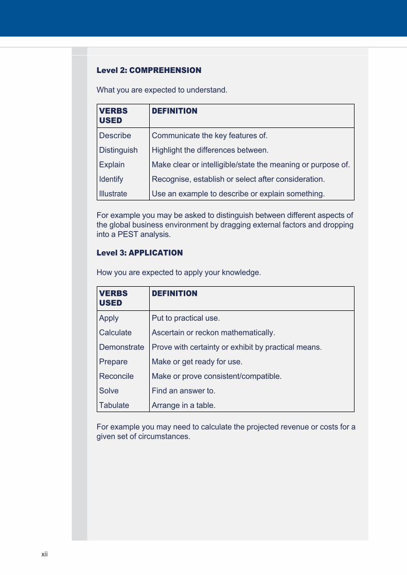
Traditional costing Chapter learning objectives

Lead Component

A1. Discuss costing methods and their results.

(a) Apply marginal (or variable) and absorption accounting methods in respect of profit reporting and stock valuation, including the reconciliation of budget and actual profit using absorption and/or marginal costing principles.

C1. Explain concepts of cost and revenue relevant to pricing and product decisions.

(c) Explain the issues that arise in pricing decisions and the conflict between ‘marginal cost’ principles and the need for full recovery of all costs incurred.

1

chapter

1

1 Chapter overview diagram

2 The purpose of costing

In the first few chapters of the syllabus we examine different techniques for determining the total costs of products and services. It’s therefore useful to remind ourselves why we might need to know this cost.

How can we calculate the cost per unit?

So we know why it’s so important for the business to determine the cost of its products or services. We now need to consider how we can calculate this cost.

• Inventory valuation – the cost per unit can be used to value inventory in the statement of financial position (balance sheet).

• To record costs – the costs associated with the product need to be recorded in the statement of profit or loss.

• To price products – the business may use the cost per unit to assist in pricing the product or service. For example, if the cost per unit is $0.30, the business may decide to price the product at $0.50 per unit in order to make the required profit of $0.20 per unit.

• Decision making – the business may use the cost information to make important decisions regarding which products or services should be made/offered and in what quantities.

Traditional costing

22

Many factors affect the level of costs incurred; for instance, inflation will cause costs to increase over a period of time. In management accounting, when we talk about cost behaviour we are referring to the way in which costs are affected by fluctuations in the level of activity. The level of activity can be measured in many different ways. For example, we can record the number of units produced, miles travelled, hours worked, percentage of capacity utilised and so on.

An understanding of cost behaviour patterns is essential for many management tasks, particularly in the areas of planning, decision­making and control. It would be impossible for managers to forecast and control costs without at least a basic knowledge of the way in which costs behave in relation to the level of activity.

In this section, we will look at the most common cost behaviour patterns and we will consider some examples of each.

Fixed cost

The CIMA Terminology defines a fixed cost as ‘a cost which is incurred for an accounting period that, within certain output or turnover limits, tends to be unaffected by fluctuations in the levels of activity (output or turnover)’.

Another term which can be used to refer to a fixed cost is ‘period cost’. This highlights the fact that a fixed cost is incurred according to the time elapsed, rather than according to the level of activity.

Examples of fixed costs are rent, rates, insurance and executive salaries.

However, it is important to note that this is only true for the relevant range of activity. Consider, for example, the behaviour of the rent cost. Within the relevant range it is possible to expand activity without needing extra premises and therefore the rent cost remains constant. However, if activity is expanded to the critical point where further premises are needed, then the rent cost will increase to a new, higher level. This cost behaviour pattern can be described as a stepped fixed cost. The cost is constant within the relevant range for each activity level but when a critical level of activity is reached, the total cost incurred increases to the next step.

chapter 1

3

Revision of cost behaviour

This warning does not only apply to fixed costs: it is never wise to attempt to predict costs for activity levels outside the range for which cost behaviour patterns have been established.

Also, whilst the fixed cost total may stay the same within a relevant activity range, the fixed cost per unit reduces as the activity level is increased. This is because the same amount of fixed cost is being spread over an increasing number of units.

Variable cost

The CIMA Terminology defines a variable cost as a 'cost that varies with a measure of activity’.

Examples of variable costs are direct material, direct labour and variable overheads. In most examination situations, and very often in practice, variable costs are assumed to be linear.

Although many variable costs do approximate to a linear function, this assumption may not always be realistic. Non­linear variable costs are sometimes called curvilinear variable costs. There may be what are known as economies of scale whereby each successive unit of activity adds less to total variable cost than the previous unit. An example of a variable cost which follows this pattern could be the cost of direct material where quantity discounts are available.

On the other hand, there may be what are known as diseconomies of scale which indicates that each successive unit of activity is adding more to the total variable cost than the previous unit. An example of a variable cost which follows this pattern could be the cost of direct labour where employees are paid an accelerating bonus for achieving higher levels of output.

The important point is that managers should be aware of any assumptions that have been made in estimating cost behaviour patterns. They can then use the information which is based on these assumptions with a full awareness of its possible limitations.

Semi­variable cost

A semi­variable cost is also referred to as a semi­fixed, hybrid, or mixed cost. The CIMA Terminology defines it as ‘a cost containing both fixed and variable components and thus partly affected by a change in the level of activity’.

Traditional costing

4

Examples of semi­variable costs are gas and electricity. Both of these expenditures consist of a fixed amount payable for the period, with a further variable amount which is related to the consumption of gas or electricity.

Alternatively, The cost might remain constant up to a certain level of activity and then increase as the variable cost element is incurred. An example of such a cost might be the rental cost of a photocopier where a fixed rental is paid and no extra charge is made for copies up to a certain number. Once this number of copies is exceeded, a constant charge is levied for each copy taken.

3 Absorption costing

The aim of traditional absorption costing is to determine the full production cost per unit.

When we use absorption costing to determine the cost per unit, we focus on the production costs only. We can summarise these costs into a cost card:

$ Direct materials per unit X Direct labour per unit X Production overhead per unit (Note 1) X

— Full production cost per unit X

—

chapter 1

5

Note 1:

All production overheads must be absorbed into units of production, using a suitable basis, e.g. units produced, labour hours or machine hours. The assumption underlying this method of absorption is that overhead expenditure is connected to the volume produced.

If, for example, units produced are used as the basis, the absorption rate is calculated as:

Total overhead cost (allocated and apportioned) –––––––––––––––––––––––––––––––––––––

Budgeted production volume

A company accountant has gathered together some cost information for her company's product as follows:

She has also determined that fixed production overheads will be $400,000 in total. Overheads are absorbed on a per unit basis.

Investigation has shown that each unit of the product uses 3 kilograms of material and needs 2 hours of direct labour work.

Sales and production were budgeted at 20,000 units, but only 16,000 were actually produced and 14,000 actually sold.

There was no opening inventory.

Required:

Produce a standard cost card using absorption costing and value the company's closing inventory on that basis.

Cost Direct materials $4 per kilogram (kg) used Direct labour $22 per hour worked Variable overheads $6 for each hour that direct labour work

Traditional costing

6

Example 1

It is relatively easy to estimate the cost per unit for direct materials and labour. In doing so we can complete the first two lines of the cost card. However, it is much more difficult to estimate the production overhead per unit. This is an indirect cost and so, by its very nature, we do not know how much is contained in each unit. Therefore, we need a method of attributing the production overheads to each unit.

Review of overhead absorption procedure

Accounting for overhead costs in an absorption costing system can be quite complex, and production overhead costs are first allocated, then apportioned and finally absorbed into production costs (or service costs).

When the department produces a single product, production volume can be measured as the number of units produced, and the absorption rate would be a rate per unit produced.

• Overhead allocation. Indirect production costs are initially allocated to cost centres or cost codes. Allocation is the process of charging a cost directly and in full to the source of the expenditure. For example, the salary of a maintenance engineer would be allocated to the engineering maintenance department.

• Overhead apportionment. The overhead costs that have been allocated to cost centres and cost codes other than direct production departments must next be apportioned to direct production departments. Apportionment is the process of sharing on a fair basis. For example, factory rental costs might be apportioned between the production departments on the basis of the floor area occupied by each department. Similarly, the costs of the engineering maintenance department might be apportioned between production departments on the basis of the operating machine hours in each department. At the end of the apportionment process, all the production overheads have been allocated or apportioned to the direct production departments.

• Overhead absorption. An absorption rate is calculated for each production department. This is the rate at which production overheads will be added to the cost of production going through the department.

chapter 1

7

More on calculating absorption rates

More usually, organisations produce different products or carry out non­standard jobs for customers, and production volume is commonly measured as one of the following:

Predetermined absorption rates

Although it is possible to calculate absorption rates using actual overhead costs and actual production volume, this is not the usual practice. This is because:

The normal practice is therefore to absorb production overhead costs at a predetermined rate, based on budgeted overhead expenditure and budgeted production volume.

This however can lead to an over­or under­absorption of the overheads when compared to the actual overheads incurred.

This over­or under­absorption can be calculated as follows:

= (Budgeted overhead rate per unit × actual units) – Actual overheads incurred

• direct labour hours worked in the department, and the absorption rate is a rate per direct labour hour worked

• machine hours worked in the department, and the absorption rate is a rate per machine hour operated

• sometimes the cost of direct labour might be used as a measure of production volume, and the absorption rate is then calculated as a percentage of direct labour cost.

• It is usually inconvenient to wait until the end of an accounting period to work out what the absorption rates should be. In absorption costing systems, overhead costs are added to the cost of production as it passes through each stage in the production process, and overhead costs are absorbed when the production happens.

• A predetermined rate is required to enable a price to be estimated.

• Overhead costs may vary throughout the year. The overhead absorption rate smoothes variations in overheads by applying an average overhead cost to each unit of product throughout the year.

Traditional costing

8

Advantages of absorption costing

The arguments used in favour of absorption costing are as follows:

Disadvantages of absorption costing

There are serious disadvantages with using absorption costing to measure costs and profits.

The way in which overhead costs are apportioned between cost centres and absorbed into production costs is subjective and many methods of cost allocation may be deemed appropriate. Although the process attempts to be ‘fair’, it is arbitrary.

• Fixed production costs can be a large proportion of the total production costs incurred. Unless production overheads are absorbed into product costs, a large proportion of cost would be excluded from the measurement of product costs.

• Absorption costing follows the matching concept (accruals concept) by carrying forward a proportion of the production cost in the inventory valuation to be matched against the sales value when the items are sold.

• It is necessary to include fixed production overhead in inventory values for financial statements; absorption costing produces inventory values which include a share of fixed production overhead.

• Analysis of under­/over­absorbed overhead may be useful for identifying inefficient utilisation of production resources.

• There is an argument that in the longer term, all costs are variable, and it is appropriate to try to identify overhead costs with the products or services that cause them. This argument is used as a reason for activity­based costing (ABC). ABC is a form of absorption costing, and is described in a later chapter.

• The apportionment and absorption of overhead costs is arbitrary

chapter 1

9

Absorption advantages/disadvantages

For example, suppose that a factory rental cost is apportioned between production departments on the basis of the floor area for each department. This might seem a fair way of sharing out the costs, but it is still subjective. Why not apportion the costs on the basis of the number of employees in each department? Or why not allow for the fact that some of the accommodation might be more pleasant to work in than others? In a manufacturing environment, production overheads might be absorbed on the basis of either direct labour hours or machine hours. However, choosing one instead of the other can have a significant effect on job costs or product costs, and yet it still relies on a subjective choice.

It may be easier in some departments than others. If a department is labour intensive then allocations can be made on the basis of labour hours worked. Or if the department is machine intensive then allocations can be made on the basis of machine hours. But not every department will have this clear distinction.

A second criticism of absorption costing is that profits can be increased or reduced by changes in inventory levels. For example, by increasing output, more fixed overhead is absorbed into production costs, and if the extra output is not sold, the fixed overhead costs are carried forward in the closing inventory value. This can encourage managers to over­produce in order to inflate profits.

• Profits vary with changes in production volume

4 Marginal costing

Marginal costing is a costing method which charges products or services with variable costs alone. The fixed costs are treated as period costs and are written off in total against the contribution of the period.

Marginal cost

Marginal cost is the extra cost arising as a result of producing one more unit, or the cost saved as a result of producing one less unit. It comprises:

• Direct material

• Direct labour

• Variable overheads

Traditional costing

10

Use the same data as that provided in Example 1.

Required:

Produce a standard cost card using marginal costing and value the company's closing inventory on that basis.

Advantages of marginal costing

Disadvantages of marginal costing

• It is a simpler costing system, because there is no requirement to apportion and absorb overhead costs.

• Marginal costing reflects the behaviour of costs in relation to activity. When sales increase, the cost of sales rise only by the additional variable costs. Since most decision­making problems involve changes to activity, marginal costing information is more relevant and appropriate for short­run decision­making than absorption costing.

• Marginal costing avoids the disadvantages of absorption costing, described above.

• When fixed costs are high relative to variable costs, and when overheads are high relative to direct costs, the marginal cost of production and sales is only a small proportion of total costs. A costing system that focuses on marginal cost and contribution might therefore provide insufficient and inadequate information about costs and product profitability. Marginal costing is useful for short­term decision­making, but not for measuring product costs and profitability over the longer term.

• It could also be argued that the treatment of direct labour costs as a variable cost item is often unrealistic. When direct labour employees are paid a fixed wage or salary, their cost is fixed, not variable.

chapter 1

11

Example 2

Marginal costing advantages/disadvantages

5 Absorption and marginal costing profit statements Absorption costing format

$ $ Sales X Less: Cost of sales

Opening inventory X + Production costs X

–– X

Less: Closing inventory (X) –– (X)

–– X

(Under)/over absorption ±X ––

Gross profit X Less: Selling, distribution and admin. costs,

Variable X Fixed X

–– (X) ––

Net profit/(loss) X ––

Traditional costing

12

Marginal costing format

$ $ Sales X Less: Variable cost of sales

Opening inventory X + Variable production costs X

–– X

Less: Closing inventory (X) –– (X)

–– X

Less: Variable selling, distribution and admin. costs (X) ––

Contribution X Less: Fixed costs

Production X Selling, distribution and admin. X

–– (X) ––

Net profit/(loss) X ––

Perry Ltd makes and sells a single product with the following information:

$/unit Selling price 50 Direct material 15 Direct labour 10 Variable overhead 5

Fixed overheads are $5,000. Budgeted and actual output and sales are 1,000 units. (a) Using absorption costing:

(i) calculate the profit for the period

(ii) calculate the profit per unit.

(b) Using marginal costing: (i) calculate the contribution per unit

(ii) calculate the total contribution

(iii) calculate the profit for the period.

chapter 1

13

Example 3

6 Reconciling the profits

The differences between the two profits can be reconciled as follows:

$ Absorption costing profit X (Increase)/decrease in inventory × fixed overheads per unit (X)/X

––––– Marginal costing profit X

–––––

The profit differences are caused by the different valuations given to the closing inventories in each period. With absorption costing, an amount of fixed production overhead is carried forward in inventory to be charged against sales of later periods.

If inventories increase, then absorption costing profits will be higher than marginal costing profits. This is because some of the fixed overhead is carried forward in inventory instead of being written off against sales for the period.

If inventories reduce, then marginal costing profits will be higher than absorption costing profits. This is because the fixed overhead which had been carried forward in inventory with absorption costing is now being released to be charged against the sales for the period.

Marginal costing and absorption costing systems give the same profit when there is no change in inventories.

Profit differences in the long term

In the long term the total reported profit will be the same whichever method is used. This is because all of the costs incurred will eventually be charged against sales; it is merely the timing of the sales that causes the profit differences from period to period.

Traditional costing

14

Justification

The details are exactly the same as for Example 3, but output and sales are now 3,000 units instead of 1,000.

Calculate the profit for the period using both absorption and marginal costing? Answer the question in any way that you want.

Z Limited manufactures a single product, the budgeted selling price and variable cost details of which are as follows:

Budgeted fixed overhead costs are $60,000 per annum charged at a constant rate each month.

Budgeted production is 30,000 units per annum.

In a month when actual production was 2,400 units and exceeded sales by 180 units, identify the profit reported under absorption costing:

$ Selling price 15.00 Variable costs per unit:

Direct materials 3.50 Direct labour 4.00 Variable overhead 2.00

A $6,660

B $7,570

C $7,770

D $8,200

Profits from one period to the next can be reconciled in a similar way. For example, the difference between periods can be explained as the change in unit sales multiplied by the contribution per unit if using marginal costing.

chapter 1

15

Example 5

Example 4

Just like reconciling profits between the two accounting systems can be achieved via a proforma, similar proformas can be used for reconciling profits between one period and the next using the same accounting system as follows:

Marginal costing reconciliation

Absorption costing reconciliation

This is a little trickier as the reconciliation needs to be adjusted for any over/under­absorptions that may have occurred of fixed overheads.

Note:

You must be careful with the direction of the absorption. For example, an over­absorption in period 1 makes profit for that month higher, therefore it must be deducted to arrive at period 2’s profit. On the other hand, an over­absorption in period 2 makes period 2’s profit higher than period 1’s, therefore it must be added in the reconciliation.

$ Profit for period 1 X Increase/(decrease) in sales × contribution per unit X/(X)

––––– Profit for period 2 X

–––––

$ Profit for period 1 X Increase/(decrease) in sales × profit per unit X/(X) (Over–)/under­absorption in period 1 (X)/X Over– /(under)­absorption in period 2 X/(X)

––––– Profit for period 2 X

–––––

7 Pricing strategies based on cost

Some organisations set their selling price based on the cost of producing the product or providing the service. Often referred to as 'cost­plus pricing', this involves adding a mark­up to the total cost of the product or service in order to arrive at the selling price.

Traditional costing

16

Further explanation on reconciling profits between periods

If an organisation does use cost as the basis for pricing it has to decide whether to employ a standard mark­up or whether to vary the mark­up according to the market conditions, type of customer, etc. A standard mark­up is used by some organisations, such as government contractors and some job costing companies, but the majority of companies vary the percentage to reflect differing market conditions for their products or services.

This mark up may be influenced by factors such as:

• The amount that customers are willing to pay. For example, the product may have a high perceived value (if, say, it is in short supply) which would therefore encourage the organisation to use a higher mark up.

• The level of competition that the product will experience. If the product has many close competitors and substitutes then the organisation may be forced to use a lower mark up.

• The organisation's objectives. For example, when first trying to break into a market and gain market awareness and market share an organisation might use a lower mark up percentage.

• Alternatively, the profit mark­up may be fixed so that the company makes a specific return on capital based on a particular capacity utilisation.

Under different circumstances there may be different interpretations of what gets included in the 'cost' element of cost plus pricing. In some circumstances full cost may be used (including absorbed overheads), in other circumstances it might be more appropriate to use marginal cost.

Full cost plus pricing

Using this method, the selling price for the product is determined as follows:

So that, for example, if the full cost was $40 and the organisation was using a 15% mark up percentage then the selling price would be set at $46 (i.e. $40 × 1.15).

Selling price = Full cost per unit × (1 + mark up percentage)

chapter 1

17

Choosing the mark up percentage

Full cost can be interpreted in different ways. It will always include the full production cost, including all absorbed overheads. But some organisations may also interpret it to include sales, distribution and administration costs.

(Note: typically, the more costs that are included in the full cost then the lower that the mark up percentage used is likely to be).

A company is replacing product A with an updated version, B, and must calculate a base cost, to which will be added a mark­up in order to arrive at a selling price. The following variable costs have been established by reference to the company’s experience with product A, although they may be subject to an error margin of + or – 10 % under production conditions for B:

As the machine time for each B would be the same as for A, the company estimates that it will be able to produce the same total quantity of B as its current production of A, which is 20,000 units. 50,000 machine hours may be regarded as the relevant capacity for the purposes of absorbing fixed manufacturing overheads. Current fixed costs are $240,000 for the production facilities, $200,000 for selling and distribution, and $180,000 for administration. For costing purposes, the 20,000 units of B can be assumed to consume 10 per cent of the total selling, distribution and administration costs.

Alternative 1, using conventional absorption costing principles and building in the conservative error margin

$ Direct material 4 Direct labour (1/4 hr @ $16/hr) 4 Variable manufacturing overheads (1/4 hr of machine time @ $8/hr) 2

––– Total variable cost per unit 10

–––

$ Variable production costs (as above) 10 Add: allowance for underestimate 10% 1

––– Add: manufacturing cost 1/4 hour of machine time @ $4.80/hour ($240,000/50,000 hours)

1.2

––– Full cost 12.2

–––

Traditional costing

18

Illustration – Full cost­plus pricing

Alternative 2, as 1 but including administrative costs

Alternative 3, as 2 but including selling and distribution costs

$ Base cost as under 1 above 12.2 Add: fixed administrative costs ($180,000 × 10% = $18,000/20,000 units)

0.9

––– Full cost 13.1

–––

$ Base cost as under 2 above 13.1 Add: fixed selling and distribution costs ($200,000 × 10% = $20,000/20,000 units)

1.0

––– Full cost 14.1

––– Depending on the analysis adopted, the full cost varies from $12.2 to $14.1. The full cost rises with each alternative, as an increasing proportion of the total costs is recovered. The profit mark­up built into the pricing formula is therefore likely to fall with each alternative from 1 to 3.

A number of advantages are claimed for full cost­plus pricing:

(1) The required profit will be made if budgeted sales volumes are achieved.

(2) It is a particularly useful method in contract costing industries such as building, where a few large individual contracts can consume the majority of the annual fixed costs and the fixed costs are low in relation to the variable costs.

(3) Assuming the organisation knows its cost structures, full cost­plus is quick and cheap to employ. Its routine nature lends itself to delegation, thus saving management time.

(4) Full cost­plus pricing can be useful in justifying selling prices to customers; if costs can be shown to have increased, this strengthens the case for an increase in the selling price.

chapter 1

19

Advantages and disadvantages of full cost plus pricing

However, there are a number of problems with full cost­plus pricing:

(1) There will always be problems associated with the selection of a ‘suitable’ basis on which to charge fixed costs to individual products or services. Selling prices can show great variation, depending on the apportionment basis chosen. This can lead to over­or under­pricing relative to competitors causing the firm to either lose business or make sales at an unintentional loss.

(2) If prices are set on the basis of normal volume, and actual volume turns out to be considerably lower, overheads will not be fully recovered from sales and predicted profits may not be attainable.

(3) The mark up can be very arbitrary and may not properly account for factors such as competition levels, how much customers are willing to pay etc.

Marginal cost­plus pricing

Using this method, the selling price for the product is determined as follows:

To the accountant, marginal cost is the same as variable cost. In setting the selling price using this method a larger mark­up percentage is added because both fixed costs and profit must be covered.

It is a particularly useful method when determining a minimum acceptable selling price (for example, for a one­off product order) and this is examined in more detail in a later chapter.

Selling price = Marginal cost per unit × (1 + mark up percentage)

Some of the reasons for using marginal cost in preference to full cost are as follows:

(1) It is just as accurate as total cost­plus pricing. A larger mark­up percentage is added because both fixed costs and profit must be covered, but the uncertainty over the fixed costs per unit remains in both pricing methods.

(2) Knowledge of marginal cost gives management the option of pricing below total cost when times are bad, in order to fill capacity.

(3) It is particularly useful in pricing specific one­off contracts because it only accounts for costs which are likely to change because of the new contract. This pricing decision is covered in more detail in a later chapter.

Traditional costing

20

Benefits and problems when using marginal cost pricing

The main criticisms of marginal cost pricing are:

(4) It also recognises the existence of scarce or limiting resources. Where these are used by competing products and services it must be reflected in the selling price if profit is to be maximised. If there is a scarce or bottleneck resource the aim must be to maximise the total contribution from the limiting factor. The contribution that each alternative product or service makes from each unit of the scarce resource must be calculated and a suitable profit margin added.

(1) Like any cost based pricing method, it ignores other factors such as levels of competition, customer attitudes etc.

(2) The mark­up becomes even more arbitrary than that used in full cost plus as now it must also include a subjective element which allows for the selling price to cover fixed costs. For this reason, many accountants argue that marginal cost plus pricing should only be used for marginal (short­term or one­off) decisions.

Target return on capital

As well as determining the selling price by adding a mark­up on cost, an organisation may also set the mark­up at a level that provides a target return on the investment that has been made in the product.

The mark­up is calculated as:

The targeted return on investment is calculated as:

Targeted return on investment in the product = Total investment in the product × targeted rate of return

Profit mark­up = Targeted return on investment in the product / budgeted level of production

This method involves determining the amount of capital invested to support a product. For example, some fixed or non­current assets and certain elements of working capital such as inventory and trade receivables can be attributed to individual products.

The selling price is then set to achieve a specified return on the capital invested on behalf of the product. The following example will demonstrate how the method works.

chapter 1

21

Example 6

LG Ltd manufactures product B. Data for product B are as follows:

LG Ltd sells 1,000 units of product B each year. Product B requires an investment of $400,000 and the target rate of return on investment is 12% per annum.

Calculate the selling price for one unit of product B, to the nearest cent.

Direct material cost per unit $62 Direct labour cost per unit $14 Direct labour hours per unit 4 hours Production overhead absorption rate $16 per direct machine

hour Mark­up for non­production overhead costs

8% of total production cost

An organisation can use a similar technique to determine a selling price which provides a target return on sales. This pricing method involves determining the full cost of a cost unit and then adding a mark­up that represents a specified percentage of the final selling price.

WP Ltd manufactures product A. Data for product A are as follows:

WP Ltd requires a 15% return on sales revenue from all products.

Calculate the selling price for product A, to the nearest cent.

Direct material cost per unit $7Direct labour cost per unit $18Direct labour hours per unit 2 hours Production overhead absorption rate $6 per direct labour hour Mark­up for non­production overhead costs

5% of total production cost

Traditional costing

22

Target return on sales

Solution

*Always read the question data carefully. The 15% required return is expressed as a percentage of the sales revenue, not as a percentage of the cost.

$ per unit Direct material cost 7.00 Direct labour cost 18.00

——– Total direct cost 25.00 Production overhead absorbed (2 hours × $6) 12.00

——– Total production cost 37.00 Mark­up for non­production costs (5% × $37.00) 1.85

——– Full cost 38.85 Profit mark­up (15/85* × $38.85) 6.86

——– Selling price 45.71

——–

Profit margin

As an alternative calculation, the examiner may provide a profit margin rather than a mark­up on cost. The selling price using a profit margin can be calculated as follows:

The decision as to what gets included in the total cost (for example, whether that is the absorption or marginal cost) and the associated calculations required to get to the total cost will be the same as when using a mark­up on cost.

Selling price = Total cost ÷ (1 – required margin)

chapter 1

23

8 Chapter summary

Traditional costing

24

9 Practice questions

Scenario

Saturn, a chocolate manufacturer, produces three products:

Information relating to each of the products is as follows:

Tasks

Using traditional absorption costing, calculate the full production cost per unit and the profit per unit for each product. Explain the implications of the figures calculated.

(Time allowed: 20 minutes)

• The Sky Bar, a bar of solid milk chocolate.

• The Moon Egg, a fondant filled milk chocolate egg.

• The Sun Bar, a biscuit and nougat based chocolate bar.

Sky Bar

Moon Egg

Sun Bar

Direct labour cost per unit ($) 0.07 0.14 0.12 Direct material cost per unit ($) 0.17 0.19 0.16 Actual production/sales (units) 500,000 150,000 250,000 Direct labour hours per unit 0.001 0.01 0.005 Direct machine hours per unit 0.01 0.04 0.02 Selling price per unit ($) 0.50 0.45 0.43 Annual production overhead = $80,000

chapter 1

25

Test your understanding 1

E plc operates a marginal costing system. For the forthcoming year, variable costs are budgeted to be 60% of sales value and fixed costs are budgeted to be 10% of sales value.

If E plc increases its selling prices by 10%, but if fixed costs, variable costs per unit and sales volume remain unchanged, identify the effect on E plc's contribution:

A a decrease of 2%

B an increase of 5%

C an increase of 10%

D an increase of 25%

When comparing the profits reported under marginal and absorption costing during a period when the level of inventories increased, identify which of the following statements would be true:

A absorption costing profits will be higher and closing inventory valuations lower than those under marginal costing

B absorption costing profits will be higher and closing inventory valuations higher than those under marginal costing

C marginal costing profits will be higher and closing inventory valuations lower than those under absorption costing

D marginal costing profits will be lower and closing inventory valuations higher than those under absorption costing

Traditional costing

26

Test your understanding 2

Test your understanding 3

Exe Limited makes a single product whose total cost per unit is budgeted to be $45. This includes fixed cost of $8 per unit based on a volume of 10,000 units per period. In a period, sales volume was 9,000 units, and production volume was 11,500 units. The actual profit for the same period, calculated using absorption costing, was $42,000.

If the profit statement were prepared using marginal costing, identify the profit for the period:

A $10,000

B $22,000

C $50,000

D $62,000

Scenario

Keats plc commenced business on 1 March making one product only, the standard cost of which is as follows:

The fixed production overhead figure has been calculated on the basis of a budgeted normal output of 36,000 units per annum.

You are to assume that actual fixed overheads were as expected and that all the budgeted fixed expenses are incurred evenly over the year. March and April are to be taken as equal period months.

$ Direct labour 5 Direct material 8 Variable production overhead 2 Fixed production overhead 5

–– Standard production cost 20

––

chapter 1

27

Test your understanding 5

Test your understanding 4

Selling, distribution and administration expenses are:

The selling price per unit is $35 and the number of units produced and sold were:

Tasks

(Time allowed: 20 minutes)

Fixed $120,000 per annum Variable 15% of the sales value

March April (units) (units)

Production 2,000 3,200 Sales 1,500 3,000

(a) prepare profit statements for each of the months of March and April using: (i) absorption costing, and

(ii) marginal costing

(b) prepare a reconciliation of the profit or loss figures given in your answers to (a)(i) and (a)(ii) accompanied by a brief explanation.

If inventory levels have increased during the period, the profit calculated using marginal costing would be _____ (choose between 'higher' and 'lower') than the profit when compared with that calculated using absorption costing.

Identify which of the following statements would be true: fixed production overheads will always be under­absorbed when:

A actual output is lower than budgeted output

B actual overheads incurred are lower than budgeted overheads

C overheads absorbed are lower than those budgeted

D overheads absorbed are lower than those incurred

Traditional costing

28

Test your understanding 6

Test your understanding 7

A company uses a standard absorption costing system. The fixed overhead absorption rate is based on labour hours. Extracts from the company’s records for last year were as follows:

The ______ (choose between 'over' and 'under') ­absorbed fixed production overheads for the year were $______ (fill in the value).

Budget Actual Fixed production overhead $450,000 $475,000 Output 50,000 units 60,000 units Labour hours 900,000 930,000

GY Ltd budgets to produce and sell 3,800 units of product R in the forthcoming year. The amount of capital investment attributable to product R will be $600,000 and GY Ltd requires a rate of return of 15% on all capital invested.

Further details concerning product R are as follows:

Fixed overhead is absorbed at a rate of $11 per machine hour.

Required:

Calculate all answers to the nearest cent.

Direct material cost per unit $14 Direct labour cost per unit $19 Variable overhead cost per unit $3 Machine hours per unit 8

(a) The variable cost of product R is $ per unit.

(b) The total (full) cost of product R is $ per unit.

(c) The selling price of product R which will achieve the specified return on investment is $ per unit.

chapter 1

29

Test your understanding 8

Test your understanding 9

A company manufactures a range of products one of which, product Y, incurs a total cost of $20 per unit. The company incurs a total cost of $600,000 each period and the directors wish to achieve a return of 18% on the total capital of $800,000 invested in the company.

Required:

Based on this information the cost­plus selling price of one unit of product Y should be $ .

Scenario

ML is an engineering company that specialises in providing engineering facilities to businesses that cannot justify operating their own facilities in­house. ML employs a number of engineers who are skilled in different engineering techniques that enable ML to provide a full range of engineering facilities to its customers.

Most of the work undertaken by ML is unique to each of its customers, often requiring the manufacture of spare parts for its customers’ equipment, or the building of new equipment from customer drawings. As a result most of ML’s work is short­term, with some jobs being completed within hours while others may take a few days.

To date, ML has adopted a cost plus approach to setting its prices. This is based upon an absorption costing system that uses machine hours as the basis of absorbing overhead costs into individual job costs. The Managing Director is concerned that, over recent months, ML has been unsuccessful when quoting for work with the consequence that there has been an increase in the level of unused capacity. It has been suggested that ML should adopt an alternative approach to its pricing based on marginal costing since ‘any price that exceeds variable costs is better than no work’.

Traditional costing

30

Test your understanding 10

Test your understanding 11

Tasks

With reference to the above scenario:

(Time allowed: 20 minutes)

(a) briefly explain absorption and marginal cost approaches to pricing

(b) discuss the validity of the comment ‘any price that exceeds variable costs is better than no work’.

chapter 1

31

Test your understanding answers

Standard cost card

Note:

Production overhead per unit in the standard cost card should be based on budgeted production. Therefore in this example they will be ($400,000/20,000 units =) $20 per unit.

Inventory valuation

If 16,000 units were produced and 14,000 units sold then there will be 2,000 units in closing inventory.

Valuing that inventory at the absorption cost will give a value of

= 2,000 × $88

= $176,000

$ Direct materials per unit 3 kgs × $4/kg 12 Direct labour per unit 2 hrs × $22/hr 44 Variable overheads 2 hrs × $6/hr 12 Production overhead per unit (note) 20

— Full/absorption cost per unit 88

—

Traditional costing

32

Example 1

Standard cost card

Note:

Fixed production overhead is not included in a marginal costing standard cost card.

Inventory valuation

Valuing that inventory at the marginal cost will give a value of

= 2,000 × $68

= $136,000

$ Direct materials per unit 3 kgs × $4/kg 12 Direct labour per unit 2 hrs × $22/hr 44 Variable overheads 2 hrs × $6/hr 12

— Marginal cost per unit 68

—

(a) (i)

$ $ Sales 1,000 units × $50 50,000 Direct materials 1,000 units × $15 15,000 Direct labour 1,000 units × $10 10,000 Variable overheads 1,000 units × $5 5,000 Fixed overheads 5,000

–––––– 35,000 ––––––

Profit 15,000 ––––––

chapter 1

33

Example 2

Example 3

The two systems give the same profit provided there is no change in inventory.

(ii)$15000

Profit per unit = ––––––– = 15/unit 1,000 units

(b) (i) Contribution per unit = $50 – ($15 + $10 + $5) = $20

(ii) Total contribution = $20/unit × 1,000 units = $20,000

(iii) $

Contribution$20/unit × 1,000 units 20,000 Fixed cost 5,000

–––––– Profit 15,000

––––––

Either marginal costing or absorption costing principles can be used. The two systems will give the same profit as there is no change in inventory (production = sales). Marginal costing will be simpler and is illustrated first.

$ Contribution

$20 per unit × 3,000 units 60,000 Fixed cost 5,000

–––––– Profit 55,000

––––––

Traditional costing

34

Example 4

Alternatively:

Notice that we did not use the $15 per unit profit figure. Unlike contribution per unit, profit per unit is not constant.

$ $ Sales 3,000 units × $50 150,000 Direct materials 3,000 units × $15 45,000 Direct labour 3,000 units × $10 30,000 Variable overheads 3,000 units × $5 15,000 Fixed overheads 3,000 units × $5 15,000

––––– (105,000)

Over­absorption of fixed overheads

($15,000 – $5,000)

10,000

–––––– 55,000 ––––––

B

A common short­cut in multiple choice questions is to calculate the marginal costing profit and then use the reconciliation of profits to get to the absorption costing profit.

First of all – the profit under marginal costing:

Contribution per unit = $15 – (3.50 + 4.00 + 2.00) = $5.50

No of units sold = 2,400 – 180 = 2,220

$ Contribution

$5.50/unit × 2,220 units 12,210 Fixed cost

$60,000 p.a./12 months 5,000 ––––– 7,210 –––––

chapter 1

35

Example 5

As production is greater than sales, absorption costing will show the higher profit.

Difference in profit = change in inventory × fixed production overhead per unit.

Difference in profit = 180 units × $2/unit = $360.

Therefore, profit reported under absorption costing = $7,210 + 360 = $7,570.

Budgeted overheads $60,000 The FOAR was worked out as ––––––––––––––– = –––––– = $2 per unit

Budgeted level of activity 30,000 units

The selling price is calculated as follows:

Working:

Target return on investment in product B = $400,000 × 12% = $48,000

Target return per unit of product B = $48,000/1,000 units = $48

$ per unit Direct material cost 62.00 Direct labour cost 14.00

——— Total direct cost 76.00 Production overhead absorbed (4 hours × $16) 64.00

——— Total production cost 140.00 Mark­up for non­production costs (8% × $140) 11.20

——— Full cost 151.20 Profit mark­up (see working) 48.00

——— Selling price 199.20

———

Traditional costing

36

Example 6

As mentioned, it is relatively easy to complete the first two lines of the cost card. The difficult part is calculating the production overhead per unit, so let’s start by considering this. We need to absorb the overheads into units of production. To do this, we will first need to calculate an overhead absorption rate (OAR):

The activity level must be appropriate for the business. Saturn must choose between three activity levels:

Working – OAR

Production overhead (this is $80,000, as per the question) OAR = —————————

Activity level (this must be chosen)

• Units of production – This would not be appropriate since Saturn produces more than one type of product. It would not be fair to absorb the same amount of overhead into each product.

• Machine hours or labour hours – It is fair to absorb production overheads into the products based on the labour or machine hours taken to produce each unit. We must decide if the most appropriate activity level is machine or labour hours. To do this we can look at the nature of the process. Production appears to be more machine intensive than labour intensive because each unit takes more machine hours to produce than it does labour hours. Therefore, the most appropriate activity level is machine hours.

OAR = $80,000 production overhead ———————————————————————(0.01 × 500k) + (0.04 × 150k) + (0.02 × 250k) hours

= $80,000 ——————16,000 hours

= $5 per machine hour

chapter 1

37

Test your understanding 1

We can now absorb these into the units of production:

This is the difficult part done. We can now quickly complete the cost card and answer the question:

Outcome of absorption costing

Based on absorption costing, the Sky Bar and the Sun Bar are both profitable. However, the Moon Egg is loss making. Managers would need to consider the future of the Moon Egg. They may look at the possibility of increasing the selling price and/or reducing costs. If this is not possible, they may make the decision to stop selling the product. However, this may prove to be the wrong decision because absorption costing does not always result in an accurate calculation of the full production cost per unit. ABC can be a more accurate method of calculating the full production cost per unit and as a result should lead to better decisions. ABC is explored in the next chapter.

Sky Bar

Moon Egg

Sun Bar

Production overheads ($) = machine hours per unit × $5

0.05

0.20

0.10

Sky Bar

Moon Egg

Sun Bar

$ $ $ Direct labour cost per unit 0.07 0.14 0.12 Direct material cost per unit 0.17 0.19 0.16 Production overhead per unit 0.05 0.20 0.10 Full production cost per unit 0.29 0.53 0.38 Selling price per unit 0.50 0.45 0.43 Profit/ (loss) per unit 0.21 (0.08) 0.05

Traditional costing

38

D

The easiest way to answer this question is to make up a number for sales, say $1,000, then the relationships will be much easier to visualise.

If sales = $1,000, then:

Variable cost = 60% × $1,000 = $600

Contribution increases by $100, which is an increase of 25% on its original value.

Fixed cost should be ignored as it does not affect contribution.

Current situation$

Sales 1,000 Variable cost 600

–––– Contribution 400

––––

New situation$

Sales (10% higher) 1,100 Variable cost 600

–––– Contribution 500

––––

B

chapter 1

39

Test your understanding 2

Test your understanding 3

B

Production is greater than sales, so absorption costing will have the higher profit.

Difference in profit = change in inventory × fixed production overhead per unit.

Difference in profit = 2,500 units × $8/unit = $20,000.

Therefore, profit reported under marginal costing = $42,000 – 20,000 = $22,000.

(a) (i)

March April $ $ $ $

Sales 52,500 105,000 Cost of sales

Op. stock (W1) 0 10,000 Production costs (@$20/unit) 40,000 64,000

——— ——— 40,000 74,000

Less cl. inventory (@$20/unit) (W2) 10,000 14,000 ——— ———

30,000 60,000 ——— ——— 22,500 45,000

(Under)/over­absorption (W3) (5,000) 1,000 ——— ———

Gross profit 17,500 46,000 Selling etc costs

Fixed (W4) 10,000 10,000 Variable 7,875 15,750

——— ——— 17,875 25,750 ——— ———

Net Profit/Loss (375) 20,250 ——— ———

Traditional costing

40

Test your understanding 5

Test your understanding 4

Workings

(ii) March April

$ $ $ $ Sales 52,500 105,000 Variable cost of sales

Op. inventory (W1) 0 7,500 Variable production costs (@$15/unit)

30,000 48,000

––––– ––––– 30,000 55,500

Less cl. inventory (@$15/unit) (W2) 7,500 10,500 ––––– –––––

22,500 45,000 ––––– ––––– 30,000 60,000

Variable selling etc costs 7,875 15,750 ––––– –––––

Contribution 22,125 44,250 Fixed costs

Production 15,000 15,000 Selling etc 10,000 10,000

––––– ––––– 25,000 25,000 ––––– –––––

Profit/Loss (2,875) 19,250 ––––– –––––

(W1) The closing inventory for March becomes the opening stock for April.

(W2) March April

Units Units Op. inventory 0 500 Production 2,000 3,200

–––– –––– 2,000 3,700

Less sales 1,500 3,000 –––– ––––

Cl. inventory 500 700

chapter 1

41

(W3) Under­/over­absorption is the difference between overheads incurred and overheads absorbed.

“Overheads incurred” means actual overheads and we are told that the actual fixed overheads were as expected. Therefore the actual fixed overheads incurred are the same as the budgeted fixed overheads.

(W4) Selling, etc fixed overhead = $120,000/12 = $10,000 per month.

Difference in profit = change in inventory × fixed production overhead cost per unit

Budgeted fixed overhead = $5 per unit × 36,000 units

= $180,000 per annum

÷ 12= 15,000 per month

March

Overheads incurred 15,000 Overheads absorbed

$5/unit × 2,000 units 10,000 –––––

Under­absorption (5,000) –––––

April

Overheads incurred 15,000 Overheads absorbed

$5/unit × 3,200 units 16,000 –––––

Over­absorption 1,000 –––––

(b) If there is no change in inventory, the 2 systems give the same profit. If production is greater than sales then absorption costing shows the higher profit.

Traditional costing

42

In both March and April, production is greater than sales and thus absorption costing will show the higher profit (the smaller loss in March).

This difference occurs because marginal costing writes off the entire fixed overhead in the period incurred, whereas absorption costing carries forward some fixed production overhead into the next period in the valuation of closing inventory.

March April Marginal costing profit/loss (2,875) 19,250 Difference in profit

(2,000 – 1,500) × $5 per unit 2,500 (3,200 – 3,000) × $5 per unit 1,000

––––– –––––– Absorption costing profit/loss (375) 20,250

––––– ––––––

Missing word: lower

Marginal costing values inventory at a lower amount because it does not include fixed overheads in the valuation. Therefore as inventory levels increase the value of closing inventory under marginal costing will be lower. This will give a higher cost of sales and a lower profit.

D Under­absorption occurs when the amount absorbed is less than the actual overheads incurred.

chapter 1

43

Test your understanding 7

Test your understanding 6

The over­absorbed fixed production overheads for the year were $65,000.

$450,000 Absorption rate = ––––––– = $0.50/hour

900,000

Absorbed overheads

60,000 units × 18 hrs/unit × $0.50/hour

= $540,000

Actual overheads = $475,000

Over­absorption = $65,000

(a) The variable cost per unit of product R is $36.00 per unit.

Direct material $14 + direct labour $19 + variable overhead $3 = $36.

Variable cost $36 + fixed overhead (8 hours × $11) = $124.

Working:

Required return from investment in product R = $600,000 × 15% = $90,000

Required return per unit sold = $90,000/3,800 units = $23.68

Required selling price = $124.00 full cost + $23.68 = $147.68

(b) The total (full) cost of product R is $124.00 per unit.

(c) The selling price of product R which will achieve the specified return on investment is $147.68 per unit.

Traditional costing

44

Test your understanding 9

Test your understanding 8

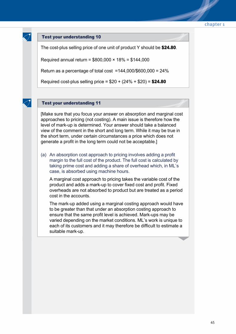
The cost­plus selling price of one unit of product Y should be $24.80.

Required annual return = $800,000 × 18% = $144,000

Return as a percentage of total cost =144,000/$600,000 = 24%

Required cost­plus selling price = $20 + (24% + $20) = $24.80

[Make sure that you focus your answer on absorption and marginal cost approaches to pricing (not costing). A main issue is therefore how the level of mark­up is determined. Your answer should take a balanced view of the comment in the short and long term. While it may be true in the short term, under certain circumstances a price which does not generate a profit in the long term could not be acceptable.]

A marginal cost approach to pricing takes the variable cost of the product and adds a mark­up to cover fixed cost and profit. Fixed overheads are not absorbed to product but are treated as a period cost in the accounts.

The mark­up added using a marginal costing approach would have to be greater than that under an absorption costing approach to ensure that the same profit level is achieved. Mark­ups may be varied depending on the market conditions. ML’s work is unique to each of its customers and it may therefore be difficult to estimate a suitable mark­up.

(a) An absorption cost approach to pricing involves adding a profit margin to the full cost of the product. The full cost is calculated by taking prime cost and adding a share of overhead which, in ML’s case, is absorbed using machine hours.

chapter 1

45

Test your understanding 10

Test your understanding 11

Care must be taken that special prices based on variable cost do not become the normal expectation or upset existing customers who are paying a price which generates a profit.

In the long run fixed cost must be covered and a profit made in accordance with company objectives. An absorption costing approach may not provide an accurate total product costs and an activity­based approach may improve the accuracy of total costs and enable ML to identify those products or customers which generate most profit.

If resources are scarce (i.e. they cannot easily be obtained at the prices or rates contained in the standard cost card) then this statement is not true, even in the short term, as scarce resources typically cost a premium and the marginal cost will increase. This concept will be explored in the decision making chapter later in the text.

(b) The comment ‘any price that exceeds variable costs is better than no work’ may have some validity in the short term. In the case of a company like ML, which has unused capacity, fixed costs will be incurred in the short term irrespective of workload, i.e. the fixed costs will not change as no extra capacity is required (for example, premises will not have to be expanded in order to accommodate the extra production), and they can therefore be ignored for decision making purposes. Any price that exceeds variable cost will provide some contribution and will reduce losses.

Traditional costing

46