Embed Size (px)
Citation preview
Chapter 53
PANEL DATA MODELS: SOME RECENT DEVELOPMENTS*
MANUEL ARELLANO
CEMFI, Casado del Alisal 5, 28014 Madrid, Spain
BO HONORE
Department of Economics, Princeton University, Princeton, New Jersey 08544
Contents
Abstract 3231Keywords 32311 Introduction 32322 Linear models with predetermined variables: identification 3233
2.1 Strict exogeneity, predeterminedness, and unobserved heterogeneity 32332.2 Time series models with error components 3241
2.2 1 The AR( 1) process with fixed effects 32422.2 2 Aggregate shocks 32452.2 3 Identification and unit roots 3246
2.2 4 The value of information with highly persistent data 32472.3 Using stationarity restrictions 32482.4 Models with multiplicative effects 3250
3 Linear models with predetermined variables: estimation 32553.1 GMM estimation 32553.2 Efficient estimation under conditional mean independence 32593.3 Finite sample properties of GMM and alternative estimators 32623.4 Approximating the distributions of GMM and LIML for AR(l) models when the number
of moments is large 32644 Nonlinear panel data models 32655 Conditional maximum likelihood estimation 3267
5.1 Conditional maximum likelihood estimation of logit models 32685.2 Poisson regression models 3269
6 Discrete choice models with "fixed" effects 3270
* We thank Jason Abrevaya, Badi Baltagi, Olympia Bover, Martin Browning, Jim Heckman, LuojiaHu, Ekaterini Kyriazidou, Ed Leamer, Aprajit Mahajan, Enrique Sentana, Jeffrey Wooldridge andparticipants at the Chicago and London Handbook conferences for helpful comments All errors are ourresponsibility.
Handbook of Econometrics, Volume 5, Edited by JJ Heckman and E Learner© 2001 Elsevier Science B V All rights reserved

3230 M Arellano and B Honor
7 Tobit-type models with "fixed" effects 32727.1 Censored regression models 3272
7.2 Type 2 Tobit model (sample selection model) 3275
7.3 Other Tobit-type models 3276
7.4 Monotone transformation models 3278
7.5 Nonparametric regression and fixed effects 3280
7.6 Relationship with estimators for some cross sectional models 3280
8 Models with lagged dependent variables 32828.1 Discrete choice with state dependence 3283
8.2 Dynamic Tobit models 3286
8.3 Dynamic sample selection models 3287
9 "Random" effects models 328710 Concluding remarks 3290References 3290
Ch 53: Panel Data Models: Some Recent Developments
Abstract
This chapter focuses on two of the developments in panel data econometrics since theHandbook chapter by Chamberlain ( 1984).
The first objective of this chapter is to provide a review of linear panel datamodels with predetermined variables We discuss the implications of assuming thatexplanatory variables are predetermined as opposed to strictly exogenous in dynamicstructural equations with unobserved heterogeneity We compare the identification frommoment conditions in each case, and the implications of alternative feedback schemesfor the time series properties of the errors We next consider autoregressive errorcomponent models under various auxiliary assumptions There is a trade-off betweenrobustness and efficiency since assumptions of stationary initial conditions or timeseries homoskedasticity can be very informative, but estimators are not robust totheir violation We also discuss the identification problems that arise in models withpredetermined variables and multiple effects Concerning inference in linear modelswith predetermined variables, we discuss the form of optimal instruments, and thesampling properties of GMM and LIML-analogue estimators drawing on Monte Carloresults and asymptotic approximations.
A number of identification results for limited dependent variable models with fixedeffects and strictly exogenous variables are available in the literature, as well as someresults on consistent and asymptotically normal estimation of such models There arealso some results available for models of this type including lags of the dependentvariable, although even less is known for nonlinear dynamic models Reviewing therecent work on discrete choice and selectivity models with fixed effects is the secondobjective of this chapter A feature of parametric limited dependent variable modelsis their fragility to auxiliary distributional assumptions This situation prompted thedevelopment of a large literature dealing with semiparametric alternatives (reviewedin Powell, 1994 's chapter) The work that we review in the second part of the chapteris thus at the intersection of the panel data literature and that on cross-sectionalsemiparametric limited dependent variable models.
Keywords
JEL classification: C 33
3231
M Arellano and B Honors
1 Introduction
Panel data analysis is at the watershed of time series and cross-section econometrics.While the identification of time series parameters traditionally relied on notions ofstationarity, predeterminedness and uncorrelated shocks, cross-sectional parametersappealed to exogenous instrumental variables and random sampling for identification.By combining the time series and cross-sectional dimensions, panel datasets haveenriched the set of possible identification arrangements, and forced economists to thinkmore carefully about the nature and sources of identification of parameters of potentialinterest.
One strand of the literature found its original motivation in the desire of exploitingpanel data for controlling unobserved time-invariant heterogeneity in cross-sectionalmodels Another strand was interested in panel data as a way to disentanglecomponents of variance and to estimate transition probabilities among states Papersin these two veins can be loosely associated with the early work on fixed andrandom effects approaches, respectively In the former, interest typically centers inmeasuring the effect of regressors holding unobserved heterogeneity constant Inthe latter, the parameters of interest are those characterizing the distributions of theerror components A third strand of the literature studied autoregressive models withindividual effects, and more generally models with lagged dependent variables.
A sizeable part of the work in the first two traditions concentrated on modelswith just strictly exogenous variables This contrasts with the situation in time serieseconometrics where the distinction between predetermined and strictly exogenousvariables has long been recognized as a fundamental one in the specification ofempirical models.
The first objective of this chapter is to review recent work on linear panel datamodels with predetermined variables Lack of control of individual heterogeneity couldresult in a spurious rejection of strict exogeneity, and so a definition of strict exogeneityconditional on unobserved individual effects is a useful extension of the standardconcept to panel data (a major theme of Chamberlain, 1984 's chapter) There are manyinstances, however, in which for theoretical or empirical reasons one is concerned withmodels exhibiting genuine lack of strict exogeneity after controlling for individualheterogeneity.
The interaction between unobserved heterogeneity and predetermined regressors inshort panels which are the typical ones in microeconometrics poses identificationproblems that are absent from both time series models and panel data models withonly strictly exogenous variables In our review we shall see that for linear models it ispossible to accommodate techniques developed from the various strands in a commonframework within which their relative merits can be evaluated.
Much less is known for discrete choice, selectivity and other non-linear models ofinterest in microeconometrics A number of identification results for limited dependentvariable models with fixed effects and strictly exogenous variables are available in theliterature, as well as some results on consistent and asymptotically normal estimation of
3232

Ch 53: Panel Data Models: Some Recent Developments
such models There are also some results available for models of this type includinglags of the dependent variable, although even less is known for nonlinear dynamicmodels.
Reviewing the recent work on discrete choice and selectivity models with fixedeffects is the second objective of this chapter A feature of parametric limited dependentvariable models is their fragility to auxiliary distributional assumptions This situationprompted the development of a large literature dealing with semiparametric alternatives(reviewed in Powell, 1994 's chapter) The work that we review in the second part of thechapter is thus at the intersection of the panel data literature and that on cross-sectionalsemiparametric limited dependent variable models.
Other interesting topics in panel data analysis which will not be covered in thischapter include work on long T panel data models with heterogeneous dynamics orunit roots lPesaran and Smith ( 1995), Canova and Marcet ( 1995), Kao ( 1999), Phillipsand Moon ( 1999)l, simulation-based random effects approaches to the nonlinearmodels lHajivassiliou and McFadden ( 1990), Keane ( 1993, 1994), Allenby and Rossi( 1999), and references thereinl, classical and Bayesian flexible estimators of errorcomponent distributions lHorowitz and Markatou ( 1996), Chamberlain and Hirano( 1999), Geweke and Keane ( 2000)l, other nonparametric and semiparametric paneldata models lBaltagi, Hidalgo and Li ( 1996), Li and Stengos ( 1996), Li and Hsiao( 1998) and Chen, Heckman and Vytlacil ( 1998)l, and models from time series ofindependent cross-sections lDeaton ( 1985), Moffitt ( 1993), Collado ( 1997)l Some ofthese topics as well as comprehensive reviews of the panel data literature are coveredin the text books by Hsiao ( 1986) and Baltagi ( 1995).
2 Linear models with predetermined variables: identification
In this section we discuss the identification of linear models with predeterminedvariables in two different contexts In Section 2 1 the interest is to identify structuralparameters in models in which explanatory variables are correlated with a time-invariant individual effect, but they are either strictly exogenous or predeterminedrelative to the time-varying errors The second context, discussed in Section 2 2, isthe time series analysis of error component models with autoregressive errors undervarious auxiliary assumptions Section 2 3 discusses the use of stationarity restrictionsin regression models, and Section 2 4 considers the identification of models withmultiplicative or multiple individual effects.
2.1 Strict exogeneity, predeterminedness, and unobserved heterogeneity
We begin with a discussion of the implications of strict exogeneity for identificationof regression parameters controlling for unobserved heterogeneity, with the objectiveof comparing this situation with that where the regressors are only predeterminedvariables.
3233
M Arellano and B Honor
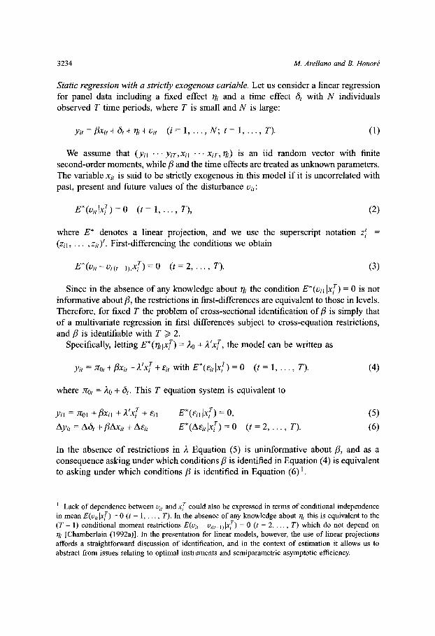
Static regression with a strictly exogenous variable Let us consider a linear regressionfor panel data including a fixed effect r/i and a time effect 6, with N individualsobserved T time periods, where T is small and N is large:
Yit =/xit+tt+i+it (i= 1, , N; t= 1, , T) ( 1)
We assume that (Yil "yir,xil Xi T, Ii) is an iid random vector with finitesecond-order moments, while fi and the time effects are treated as unknown parameters.The variable xi, is said to be strictly exogenous in this model if it is uncorrelated withpast, present and future values of the disturbance ui,:
E*(vilxi T) = O (t = 1, , T), ( 2)
where E* denotes a linear projection, and we use the superscript notation z =(zil, ,zi,)' First-differencing the conditions we obtain
E*(oit i( t )lx T) = O (t = 2, , T) ( 3)
Since in the absence of any knowledge about tri the condition E*(vil Ixi T) = O is notinformative about fi, the restrictions in first-differences are equivalent to those in levels.Therefore, for fixed T the problem of cross-sectional identification of /f is simply thatof a multivariate regression in first differences subject to cross-equation restrictions,and /i is identifiable with T 2.
Specifically, letting E*(rilx T) = Ao + t'x T, the model can be written as
Yit = Jrot + xit + xi + Eit, with E*(Eitf x T) = O (t = 1 , T) ( 4)
where r Oo, = AO + 6, This T equation system is equivalent to
Yil = j T 01 + Xil + AIX T + Eil E*(Eil Ix T) = 0, ( 5)
Ayt = At + Axit + A Eit E*(A Ei, l XT) = (t = 2, T) ( 6)
In the absence of restrictions in A Equation ( 5) is uninformative about fi, and as aconsequence asking under which conditions fi is identified in Equation ( 4) is equivalentto asking under which conditions /3 is identified in Equation ( 6) 1.
i Lack of dependence between it, and x IT could also be expressed in terms of conditional independencein mean E(vi, Ixj T) = O (t = 1, , T) In the absence of any knowledge about i this is equivalent to the(T 1) conditional moment restrictions E(u, Vi(,__l I Xr ) = O (t = 2, , T) which do not depend onij lChamberlain ( 1992 a)l In the presentation for linear models, however, the use of linear projectionsaffords a straightforward discussion of identification, and in the context of estimation it allows us toabstract from issues relating to optimal instruments and semiparametric asymptotic efficiency.
3234

Ch 53: Panel Data Models: Some Recent Developments
Partial adjustment with a strictly exogenous variable In an alternative model, the effectof a strictly exogenous x on y could be specified as a partial adjustment equation:
Yit = ayi( _) + 3 oxit + Plxi(t 1) + 6 t + i +vit (i = 1, , N; t= 2, , T) ( 7)
together with
E*(vitlx T) = O (t = 2, , T) ( 8)
Note that assumption ( 8) does not restrict the serial correlation of v, so that laggedy is an endogenous explanatory variable In the equation in levels, i(, ) will becorrelated with Iri by construction and may also be correlated with past, present andfuture values of the errors vi, since they may be autocorrelated in an unspecifiedway Likewise, the system in first differences is free from fixed effects and satifiesE*(Avitlx T) = O (t = 3, , T), but Ayi(t 1) may still be correlated with Avis for alls.
Subject to a standard rank condition, a, 30, fil and the time effects will be identifiedwith T > 3 With T = 3 they are just identified since there are five orthogonalityconditions and five unknown parameters:
El X xi2 (A Yi 3 a Ayi 2 o Axi 3 Axi 2 A 3)l = O ( 9)Xi 2Xi3
E (Yi 2 a Yil f 3 oxi 2 Xil 2) = 0.
This simple example illustrates the potential for cross-sectional identification understrict exogeneity In effect, strict exogeneity of x permits the identification of thedynamic effect of x on y and of lagged y on current y, in the presence of a fixedeffect and shocks that can be arbitrarily persistent over time lcf Bhargava and Sargan( 1983), Chamberlain ( 1982 a, 1984), Arellano ( 1990)l.
A related situation of economic interest arises in testing life-cycle models ofconsumption or labor supply with habits le g , Bover ( 1991), or Becker, Grossmanand Murphy ( 1994)l In these models the coefficient on the lagged dependent variableis a parameter of central interest as it is intended to measure the extent of habits.However, in the absence of an exogenous instrumental variable such a coefficient wouldnot be identified, since the effect of genuine habits could not be separated from serialcorrelation in the unobservables.
As an illustration, let us consider the empirical model of cigarette consumption byBecker, Grossman and Murphy ( 1994) for US state panel data Their empirical analysisis based on the following equation:
cit = Oci(t I 1) + i Oci(t + Y Pit + li + + i(t+ 1), ( 10)
where ci and pit denote, respectively, annual per capita cigarette consumption in packsby state and average cigarette price per pack Becker et al are interested in testing
3235
M Arellano and B Honors
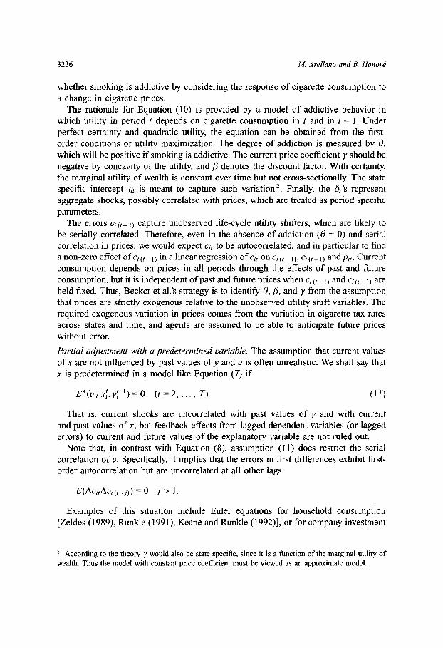
whether smoking is addictive by considering the response of cigarette consumption toa change in cigarette prices.
The rationale for Equation ( 10) is provided by a model of addictive behavior inwhich utility in period t depends on cigarette consumption in t and in t 1 Underperfect certainty and quadratic utility, the equation can be obtained from the first-order conditions of utility maximization The degree of addiction is measured by 0,which will be positive if smoking is addictive The current price coefficient y should benegative by concavity of the utility, and /3 denotes the discount factor With certainty,the marginal utility of wealth is constant over time but not cross-sectionally The statespecific intercept ii is meant to capture such variation 2 Finally, the 6,'s representaggregate shocks, possibly correlated with prices, which are treated as period specificparameters.
The errors i (t+ ) capture unobserved life-cycle utility shifters, which are likely tobe serially correlated Therefore, even in the absence of addiction ( O = 0) and serialcorrelation in prices, we would expect cit to be autocorrelated, and in particular to finda non-zero effect of ci (,t ) in a linear regression of ci, on ci(t ), ci(t+ 1) andpi Currentconsumption depends on prices in all periods through the effects of past and futureconsumption, but it is independent of past and future prices when ci (, _ ) and ci (t+ ) areheld fixed Thus, Becker et al 's strategy is to identify 0, /3, and y from the assumptionthat prices are strictly exogenous relative to the unobserved utility shift variables Therequired exogenous variation in prices comes from the variation in cigarette tax ratesacross states and time, and agents are assumed to be able to anticipate future priceswithout error.
Partial adjustment with a predetermined variable The assumption that current valuesof x are not influenced by past values of y and v is often unrealistic We shall say thatx is predetermined in a model like Equation ( 7) if
E*(vixi',y'-) = O (t = 2, , T) ( 11)
That is, current shocks are uncorrelated with past values of y and with currentand past values of x, but feedback effects from lagged dependent variables (or laggederrors) to current and future values of the explanatory variable are not ruled out.
Note that, in contrast with Equation ( 8), assumption ( 11) does restrict the serialcorrelation of v Specifically, it implies that the errors in first differences exhibit first-order autocorrelation but are uncorrelated at all other lags:
E(Avit Avi(t, )) = O j > 1.
Examples of this situation include Euler equations for household consumptionlZeldes ( 1989), Runkle ( 1991), Keane and Runkle ( 1992)l, or for company investment
2 According to the theory y would also be state specific, since it is a function of the marginal utility ofwealth Thus the model with constant price coefficient must be viewed as an approximate model.
3236
Ch 53: Panel Data Models: Some Recent Developments
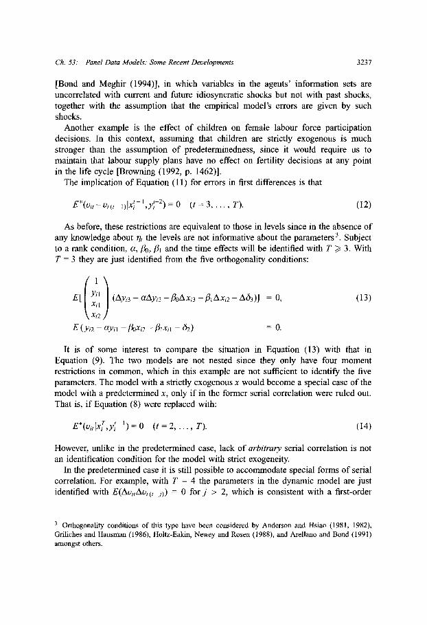
lBond and Meghir ( 1994)l, in which variables in the agents' information sets areuncorrelated with current and future idiosyncratic shocks but not with past shocks,together with the assumption that the empirical model's errors are given by suchshocks.
Another example is the effect of children on female labour force participationdecisions In this context, assuming that children are strictly exogenous is muchstronger than the assumption of predeterminedness, since it would require us tomaintain that labour supply plans have no effect on fertility decisions at any pointin the life cycle lBrowning ( 1992, p 1462)l.
The implication of Equation ( 11) for errors in first differences is that
E*(Oit i(t 1)IX ,yi-2 ) = O (t = 3, , T) ( 12)
As before, these restrictions are equivalent to those in levels since in the absence ofany knowledge about i the levels are not informative about the parameters 3 Subjectto a rank condition, a, i 0, I and the time effects will be identified with T > 3 WithT = 3 they are just identified from the five orthogonality conditions:
El yi l (AY 3 a A Yi 2 o A Xi 3 PIA Xi 2 A 63)l = 0, ( 13)
Xi 2 /E (Yi2 a Yi oxi 2 1 xil 52) = 0.
It is of some interest to compare the situation in Equation ( 13) with that inEquation ( 9) The two models are not nested since they only have four momentrestrictions in common, which in this example are not sufficient to identify the fiveparameters The model with a strictly exogenous x would become a special case of themodel with a predetermined x, only if in the former serial correlation were ruled out.That is, if Equation ( 8) were replaced with:
E*(v,lx i ,yi ) = O (t = 2 , T) ( 14)
However, unlike in the predetermined case, lack of arbitrary serial correlation is notan identification condition for the model with strict exogeneity.
In the predetermined case it is still possible to accommodate special forms of serialcorrelation For example, with T = 4 the parameters in the dynamic model are justidentified with E(Av Aitvi(, j)) = O for j > 2, which is consistent with a first-order
3 Orthogonality conditions of this type have been considered by Anderson and Hsiao ( 1981, 1982),Griliches and Hausman ( 1986), Holtz-Eakin, Newey and Rosen ( 1988), and Arellano and Bond ( 1991)amongst others.
3237
M Arellano and B Honored
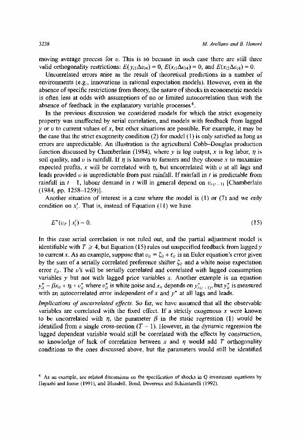
moving average process for v This is so because in such case there are still threevalid orthogonality restrictions: E(yil Avi 4) = O, E(Xil A Ui 4) = 0, and E(Xi 2A Ui 4) = 0.
Uncorrelated errors arise as the result of theoretical predictions in a number ofenvironments (e g , innovations in rational expectation models) However, even in theabsence of specific restrictions from theory, the nature of shocks in econometric modelsis often less at odds with assumptions of no or limited autocorrelation than with theabsence of feedback in the explanatory variable processes 4 .
In the previous discussion we considered models for which the strict exogeneityproperty was unaffected by serial correlation, and models with feedback from laggedy or v to current values of x, but other situations are possible For example, it may bethe case that the strict exogeneity condition ( 2) for model ( 1) is only satisfied as long aserrors are unpredictable An illustration is the agricultural Cobb-Douglas productionfunction discussed by Chamberlain ( 1984), where y is log output, x is log labor, r issoil quality, and v is rainfall If r is known to farmers and they choose x to maximizeexpected profits, x will be correlated with r 1, but uncorrelated with v at all lags andleads provided v is unpredictable from past rainfall If rainfall in t is predictable fromrainfall in t 1, labour demand in t will in general depend on vi(-_l) lChamberlain( 1984, pp 1258-1259)l.
Another situation of interest is a case where the model is ( 1) or ( 7) and we onlycondition on xt That is, instead of Equation ( 11) we have
E*(vi, x) = O ( 15)
In this case serial correlation is not ruled out, and the partial adjustment model isidentifiable with T > 4, but Equation ( 15) rules out unspecified feedback from lagged yto current x As an example, suppose that vi, = it + Eit is an Euler equation's error givenby the sum of a serially correlated preference shifter ~i, and a white noise expectationerror Ei, The vo's will be serially correlated and correlated with lagged consumptionvariables y but not with lagged price variables x Another example is an equationy = /Xit + li + Ui*t where vi is white noise and xit depends on y,*(,_ ), but y* is measuredwith an autocorrelated error independent of x and y* at all lags and leads.
Implications of uncorrelated effects So far, we have assumed that all the observablevariables are correlated with the fixed effect If a strictly exogenous x were knownto be uncorrelated with ir, the parameter fi in the static regression ( 1) would beidentified from a single cross-section (T = 1) However, in the dynamic regression thelagged dependent variable would still be correlated with the effects by construction,so knowledge of lack of correlation between x and would add T orthogonalityconditions to the ones discussed above, but the parameters would still be identified
4 As an example, see related discussions on the specification of shocks in Q investment equations byHayashi and Inoue ( 1991), and Blundell, Bond, Devereux and Schiantarelli ( 1992).
3238

Ch 53: Panel Data Models: Some Recent Developments
only when T 35 The moment conditions for the partial adjustment model withstrictly exogenous x and uncorrelated effects can be written as
El x T (yit yi(t )-f 3 oxitf -Pl Xi(tl)-) t)l =O (t= 2, , T) ( 16)
A predetermined x could also be known to be uncorrelated with the fixed effects iffeedback occurred from lagged errors but not from lagged y To illustrate this pointsuppose that the process for x is
Xit =pxi(t 1) + yi(t 1) + O r 1 i + Eit, ( 17)
where eit, vis and ri are mutually uncorrelated for all t and s In this example x isuncorrelated with when = O However, if i(t 1) were replaced by Yi (t-) inEquation ( 17), x and 71 will be correlated in general even with O = O Knowledge oflack of correlation between a predetermined x and would also add T orthogonalityrestrictions to the ones discussed above for such a case The moment conditions forthe partial adjustment model with a predetermined x uncorrelated with the effects canbe written as
El(l,) lx = O (t= 2, , T),( 18)E 1 )(Yit ayi(t ) foxit li (t 1) -t) = 2
Ely -2 (Ayit a Ayi(t 1) f Po Axit l Axi (t 1) t)l = O (t = 3, , T).
Again, the parameters in this case would only be identified when T 3.
Relationship with statistical definitions To conclude this discussion, it may be usefulto relate our usage of strict exogeneity to statistical definitions A (linear projectionbased) statistical definition of strict exogeneity conditional on a fixed effect wouldstate that x is strictly exogenous relative to y given r if
E*(yit Ixr, ri) = E*(yitlx I, ri) ( 19)
This is equivalent to the statement that y does not Granger-cause x given r 1 in the sensethat
E*(xi (+ l) x,y, iri) = E*(xi(t+ l) xi, Ili) ( 20)
Namely, letting xit +1)T = (Xi(+ 1), , Xi T) t if we have
E*(y, Ixi, T) = 'xi + 6 txi )T + 7 t rli ( 21)
and
E* (xi (t + 1) Ix,y, i, ) = Vtxt + O Yi + t i, ( 22)
it turns out that the restrictions 6, = O and ,t = O are equivalent This result generalizedthe well-known equivalence between strict exogeneity lSims ( 1972)l and Granger's
5 Models with strictly exogenous variables uncorrelated with the effects were considered by Hausmanand Taylor ( 1981), Bhargava and Sargan ( 1983), Amemiya and Ma Curdy ( 1986), Breusch, Mizon andSchmidt ( 1989), Arellano ( 1993), and Arellano and Bover ( 1995).
3239
M Arellano and B Honor
non-causality lGranger ( 1969)l 6 It was due to Chamberlain ( 1984), and motivatedthe analysis in Holtz-Eakin, Newey and Rosen ( 1988), which was aimed at testingsuch a property.
Here, however, we are using strict exogeneity relative to the errors of an econometricmodel Strict exogeneity itself, or the lack of it, may be a property of the modelsuggested by theory We used some simple models as illustrations, in the understandingthat the discussion would also apply to models that may include other featureslike individual effects uncorrelated with errors, endogenous explanatory variables,autocorrelation, or constraints in the parameters Thus, in general strict exogeneityrelative to a model may or may not be testable, but if so we shall usually be ableto test it only in conjunction with other features of the model In contrast with theeconometric concept, a statistical definition of strict exogeneity is model free, butwhether it is satisfied or not, may not necessarily be of relevance for the econometricmodel of interest 7.
As an illustration, let us consider a simple permanent-income model The observ-ables are non-durable expenditures cit, current income wit, and housing expenditure xi,.The unobservables are permanent (wlp) and transitory (it) income, and measurementerrors in non-durable (it) and housing (it) expenditures The expenditure variablesare assumed to depend on permanent income only, and the unobservables are mutuallyindependent but can be serially correlated With these assumptions we have
wit = wit + Eit, ( 23)
cit = f/wtp + it, ( 24)
xit = ywi, + i, ( 25)
Suppose that /3 is the parameter of interest The relationship between cit and witsuggested by the theory is of the form
Cit = 3wit + vii, ( 26)
where uit = it P Eit Since Wit and ,it are contemporaneously correlated, Wit is anendogenous explanatory variable in Equation ( 26) Moreover, since E*(it Ix T) = O, xi,is a strictly exogenous instrumental variable in Equation ( 26) At the same time, note
6 If linear projections are replaced by conditional distributions, the equivalence does not hold and it turnsout that the definition of Sims is weaker than Granger's definition Conditional Granger non-causalityis equivalent to the stronger Sims' condition given by f(y,Ixr,y ) = f(y,lx',y' 1) lChamberlain( 1982 b)l.7 Unlike the linear predictor definition, a conditional independence definition of strict exogeneity givenan individual effect is not restrictive, in the sense that there always exists a random variable r 1 suchthat the condition is satisfied lChamberlain ( 1984)l This lack of identification result implies that aconditional-independence test of strict exogeneity given an individual effect will necessarily be a jointtest involving a (semi) parametric specification of the conditional distribution.
3240

Ch 53: Panel Data Models: Some Recent Developments
that in general linear predictors of x given its past can be improved by adding laggedvalues of c and/or W (unless permanent income is white noise) Thus, the statisticalcondition for Granger non-causality or strict exogeneity is not satisfied in this example.A similar discussion could be conducted for a version of the model including fixedeffects.
2.2 Time series models with error components
The motivation in the previous discussion was the identification of regression responsesnot contaminated from heterogeneity biases Another leading motivation for usingpanel data is the analysis of the time series properties of the observed data Modelsof this kind were discussed by Lillard and Willis ( 1978), Ma Curdy ( 1982), Hall andMishkin ( 1982), Holtz-Eakin, Newey and Rosen ( 1988) and Abowd and Card ( 1989),amongst others.
An important consideration is distinguishing unobserved heterogeneity from genuinedynamics For example, the exercises cited above are all concerned with thetime series properties of individual earnings for different reasons, including theanalysis of earnings mobility, testing the permanent income hypothesis, or estimatingintertemporal labour supply elasticities However, how much dependence is measuredin the residuals of the earnings process depends crucially, not only on how muchheterogeneity is allowed into the process, but also on the auxiliary assumptions made inthe specification of the residual process, and assumptions about measurement errors.
One way of modelling dynamics is through moving average processes le g , Abowdand Card ( 1989)l These processes limit persistence to a fixed number of periods,and imply linear moment restrictions in the autocovariance matrix of the data.Autoregressive processes, on the other hand, imply nonlinear covariance restrictionsbut provide instrumental-variable orthogonality conditions that are linear in theautoregressive coefficients Moreover, they are well suited to analyze the implicationsfor identification and inference of issues such as the stationarity of initial conditions,homoskedasticity, and (near) unit roots.
Another convenient feature of autoregressive processes is that they can be regardedas a special case of the regression models with predetermined variables discussedabove This makes it possible to consider both types of problems in a commonframework, and facilitates the distinction between static responses with residual serialcorrelation and dynamic responses 8 Finally, autoregressive models are more easilyextended to limited-dependent-variable models.
In the next subsection we discuss the implications for identification of alternativeassumptions concerning a first-order autoregressive process with individual effects inshort panels.
8 In general, linear conditional models can be represented as data covariance matrix structures, buttypically they involve a larger parameter space including many nuisance parameters, which are absentfrom instrumental-variable orthogonality conditions.
3241
M Arellano and B Honors
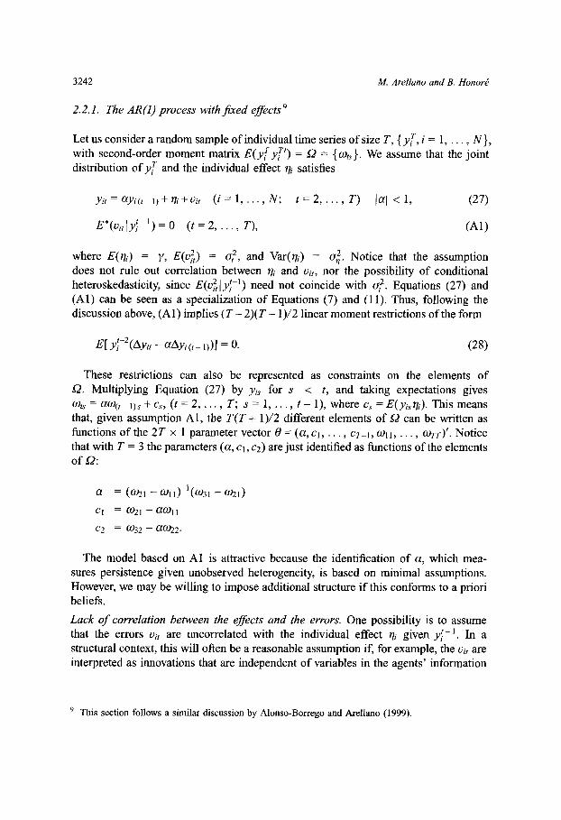
2.2 1 The AR( 1) process with fixed effects 9
Let us consider a random sample of individual time series of size T, {yr T, i = 1, , N},with second-order moment matrix E(y Tyi ) = Q = {to,} We assume that the jointdistribution of yr and the individual effect i satisfies
yit = yi( , )i + Uit (i = 1, , N; t = 2, , T) lai < 1, ( 27)
E*(vity l) = O (t = 2, , T), (Al)
where E(h) = y, E(v 2) = a 2, and Var(/li) = 2 Notice that the assumptiondoes not rule out correlation between iri and v,, nor the possibility of conditionalheteroskedasticity, since E(v 2 tly- 1 ) need not coincide with t,2 Equations ( 27) and(Al) can be seen as a specialization of Equations ( 7) and ( 11) Thus, following thediscussion above, (Al) implies (T 2)(T 1)/2 linear moment restrictions of the form
El y-2 (Ayit a Ayi(t_ 1))l = O ( 28)
These restrictions can also be represented as constraints on the elements ofQ Multiplying Equation ( 27) by yis for S < t, and taking expectations gives(ts = aw(t_ )s + c,, (t = 2, , T; S = 1, , t 1), where c, = E(yisti) This meansthat, given assumption Al, the T(T + 1)/2 different elements of 2 can be written asfunctions of the 2 T x 1 parameter vector O = (a, cl, , cr-1, W 1 , , (r TT)' Noticethat with T = 3 the parameters (a, cl, c 2) are just identified as functions of the elementsof 2:
a = (w 21 wll)1 ( 31 W 21)
c = 21 -ac 11
C 2 = 32 a 0)2 2 .
The model based on Al is attractive because the identification of a, which mea-sures persistence given unobserved heterogeneity, is based on minimal assumptions.However, we may be willing to impose additional structure if this conforms to a prioribeliefs.
Lack of correlation between the effects and the errors One possibility is to assumethat the errors voi, are uncorrelated with the individual effect th 7 given y-' In astructural context, this will often be a reasonable assumption if, for example, the v, areinterpreted as innovations that are independent of variables in the agents' information
9 This section follows a similar discussion by Alonso-Borrego and Arellano ( 1999).
3242
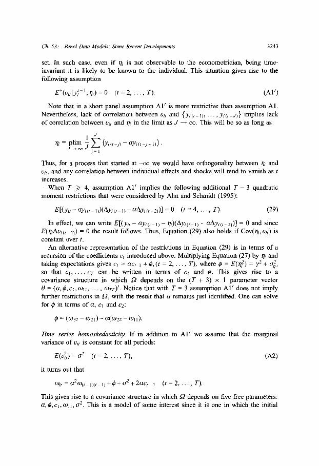
Ch 53: Panel Data Models: Some Recent Developments
set In such case, even if i is not observable to the econometrician, being time-invariant it is likely to be known to the individual This situation gives rise to thefollowing assumption
E* (vi, y'-l, ) = O (t = 2, , T) (Al')
Note that in a short panel assumption Al' is more restrictive than assumption Al.Nevertheless, lack of correlation between vi, and {yi(t 1) , y, i(t-J)} implies lackof correlation between vi, and i in the limit as J o This will be so as long as
ni = plim E (Yi( j) -ayi(,t -l))J j= 1
Thus, for a process that started at -oo we would have orthogonality between /i andui,, and any correlation between individual effects and shocks will tend to vanish as tincreases.
When T 4, assumption Al' implies the following additional T 3 quadraticmoment restrictions that were considered by Ahn and Schmidt ( 1995):
El(yit ayi(t, ))(Ayi(t ) a Ayi(t 2))l = O (t = 4, , T) ( 29)
In effect, we can write El(yit ayi(, 1) ri)(Ayi(t I) a Ayi(t- 2))l = O and sinceE( 7 i Alvi(,-1)) = O the result follows Thus, Equation ( 29) also holds if Cov(r 7 i, vit) isconstant over t.
An alternative representation of the restrictions in Equation ( 29) is in terms of arecursion of the coefficients c, introduced above Multiplying Equation ( 27) by 1 ri andtaking expectations gives c, = act i + q, (t = 2, , T), where O = E(qi 2) = 2 + 2so that cl, , cr can be written in terms of cl and This gives rise to acovariance structure in which Q 2 depends on the (T + 3) x 1 parameter vector0 = (a, 0, cl, wol, , cow )' Notice that with T = 3 assumption Al' does not implyfurther restrictions in 2, with the result that a remains just identified One can solvefor p in terms of a, cl and 2:
¢ = (( 032 ( 021) a(( 02 2 ( 011).
Time series homoskedasticity If in addition to Al' we assume that the marginalvariance of vii is constant for all periods:
E(v 2) = a 2 (t= 2, , T), (A 2)
it turns out that
tt = a 2 (t _ )( 1) + + 2 + 2 ac, 1 (t = 2, , T).
This gives rise to a covariance structure in which Q depends on five free parameters:a, 0, cl, W 1 , a 2 This is a model of some interest since it is one in which the initial
3243
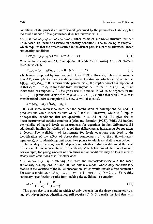
M Arellano and B Honors
conditions of the process are unrestricted (governed by the parameters O and cl), butthe total number of free parameters does not increase with T.
Mean stationarity of initial conditions Other forms of additional structure that canbe imposed are mean or variance stationarity conditions The following assumption,which requires that the process started in the distant past, is a particularly useful meanstationarity condition:
Cov(yi, -yi(t 1), ri) = O (t = 2, , T) (B 1)
Relative to assumption Al, assumption Bl adds the following (T 2) momentrestrictions on 2:
El(yit ayi(t 1))Ayi(t 1)l = 0 (t = 3, T), ( 30)
which were proposed by Arellano and Bover ( 1995) However, relative to assump-tion Al', assumption Bl only adds one moment restriction which can be written asEl(Yi 3 a Yi 2)A Yi 2 l = O In terms of the parameters ct, the implication of assumption B 1is that cl = = CT if we move from assumption Al, or that cl = 0/(l a) if wemove from assumption Al' This gives rise to a model in which Q 2 depends on the(T + 2) x I parameter vector O = (a, , wll , TT)' Notice that with T = 3, a isoveridentified under assumption B 1 Now a will also satisfy
a = ( 0)22 W)21)-1 ( 0)32 0)31).
It is of some interest to note that the combination of assumptions Al and B 1produces the same model as that of Al' and B 1 However, while Al' impliesorthogonality conditions that are quadratic in a, Al or Al+B 1 give rise tolinear instrumental-variable conditions lAhn and Schmidt ( 1995)l While Al impliedthe validity of lagged levels as instruments for equations in first-differences, Bladditionally implies the validity of lagged first-differences as instruments for equationsin levels The availability of instruments for levels equations may lead to theidentification of the effect of observable components of r 1 i (i e , time-invariantregressors), or to identifying unit roots, two points to which we shall return below.
The validity of assumption Bl depends on whether initial conditions at the startof the sample are representative of the steady state behaviour of the model or not.For example, for young workers or new firms initial conditions may be less related tosteady state conditions than for older ones.
Full stationarity By combining Al' with the homoskedasticity and the meanstationarity assumptions, A 2 and B 1, we obtain a model whose only nonstationaryfeature is the variance of the initial observation, which would remain a free parameter.For such a model 0)tt = a 20)(t l)(t 1) + a 2 + $( 1 + a)/(l a) (t = 2, , T) A fullystationary specification results from making the additional assumption:
0 __a 2
( 1 a)2 ( 1 a 2) (B 2)
This gives rise to a model in which Q 2 only depends on the three parameters a, ¢,and ar 2 Nevertheless, identification still requires T 3, despite the fact that with
3244

Ch 53: Panel Data Models: Some Recent Developments
T = 2, Q 2 has three different coefficients To see this, note that in their relationship toa, ¢, and a 02 the equation for the second diagonal term is redundant:
(Ot = 6 + 2 (t = 1,2), 0)12 = a(, 2 ) + 2 ,
where a 2 = o,2/(l a)2 and a 2 = 2/( 1 a 2 ) The intuition for this is that bothr 7 h and yi(, ) induce serial correlation on yit, but their separate effects can only bedistinguished if at least first and second order autocorrelations are observed.
Under full stationarity (assumptions Al, A 2, B 1, and B 2) it can be shown that
E(Ayi(t+l)Ayit) ( a)
El(Ayit)2 l 2
This is a well-known expression for the bias of the least squares regression in first-differences under homoskedasticity, which can be expressed as the orthogonalityconditions
E{Ayitl( 2 yi(t+ ) -yit -yi(t )) a Ayitl} = O (t = 2, , T 1).
With T = 3 this implies that a would also satisfy
a = ( 2 2 + c 11 20 21 )-1 l 2 (W 032 0)3 1 )+ 011 0)22 l
2.2 2 Aggregate shocks
Under assumptions Al or Al', the errors ,it are idiosyncratic shocks that are assumedto have cross-sectional zero mean at each point in time However, if vt containsaggregate shocks that are common to all individuals its cross-sectional mean will notbe zero in general This suggests replacing Al with the assumption
E*(oitlyi'-l) = 6 t (t = 2, , T), ( 31)
which leads to an extension of the basic specification in which an intercept is allowedto vary over time:
Yit = 6 t + ayi(t_ 1) + i + vt, ( 32)
where t = vit b 6 We can now set E(rj) = O without lack of generality, sincea nonzero mean would be subsumed in 6 t Again, formally Equation ( 32) is just aspecialization of Equations ( 7) and ( 11).
With fixed T, this extension does not essentially alter the previous discussionsince the realized values of the shocks bt can be treated as unknown period specific
3245
M Arellano and B Honors
parameters With T = 3, a, 62 and 63 are just identified from the three momentconditions ',
E(yi 2 62 ayyil) = 0, ( 33)
E(yi 3 3 a Yi 2) = 0, ( 34)
Ely 1 (i(Ay 3 63 a A Yi 2)l = O ( 35)
In the presence of aggregate shocks the mean stationarity condition in assumptionB 1 may still be satisfied, but it will be interpreted as an assumption of mean stationarityconditional upon an aggregate effect (which may or may not be stationary), sincenow E(Ayit) is not constant over t The orthogonality conditions in Equation ( 30)remain valid in this case with the addition of a time varying intercept With T = 3,assumption B 1 adds to Equations ( 33-35) the orthogonality condition:
ElAyi 2 (Yi 3 63 a Yi 2)l = O ( 36)
2.2 3 Identification and unit roots
If one is interested in the unit root hypothesis, the model needs to be specified underboth stable and unit roots environments We begin by considering model ( 27) underassumption Al as the stable root specification As for the unit root specification, it isnatural to consider a random walk without drift The model can be written as
Yit = ayi(,t_ ) + (I a)ni* + vit, ( 37)
where ri* denotes the steady state mean of the process when al < Thus, whena = 1 we have
Yit = Yi(t 1) + Vit, ( 38)
so that heterogeneity only plays a role in the determination of the starting point of theprocess Note that in this model the covariance matrix of (yi, r*) is left unrestricted.
An alternative unit root specification would be a random walk with an individualspecific drift given by r/i:
Yit = Yi(t 1) + i + it, ( 39)
but this is a model with heterogeneous linear growth that would be more suited forcomparisons with stationary models that include individual trends.
10 Further discussion on models with time effects is contained in Crepon, Kramarz and Trognon ( 1997).
3246
Ch 53: Panel Data Models: Some Recent Developments
The main point to notice here is that in model ( 37) a is not identified from themoments derived from assumption Al when a = 1 This is so because in the unitroot case the lagged level will be uncorrelated with the current innovation, so thatCov(yi(,_ 2 ),Ayi(t 1)) = O As a result, the rank condition will not be satisfied for thebasic orthogonality conditions ( 28) In model ( 39) the rank condition is still satisfiedsince Cov(yi(, 2),A Yi(t_ 1)) X 0 due to the cross-sectional correlation induced by theheterogeneity in shifts.
As noted by Arellano and Bover ( 1995), this problem does not arise when weconsider a stable root specification that in addition to assumption Al satisfies the meanstationarity assumption B 1 The reason is that when a = 1 the moment conditions ( 30)remain valid and the rank condition is satisfied since Cov(Ayi(t_ 1),yi (t 1)) • 0.
2.2 4 The value of information with highly persistent data
The cross-sectional regression coefficient of Yit on Yi(, 1), Pt, can be expressed as afunction of the model's parameters For example, under full stationarity it can be shownto be
Cov(ri,yi(t )) ( 1 a) 2 a ( 40)w pa+r A o Var(yi(,_-)) a 2 + ( 1 a)/(l + a)
where A = a,/a Often, empirically p is near unity For example, with firm employmentdata, Alonso-Borrego and Arellano ( 1999) found p = 0 995, a = 0 8, and A = 2 Sincefor any 0 a p there is a value of A such that p equals a pre-specified value,in view of lack of identification of a from the basic moment conditions ( 28) whena = 1, it is of interest to see how the information about a in these moment conditionschanges as T and a change for values of p close to one.
For the orthogonality conditions ( 28) the inverse of the semiparametric informationbound about a can be shown to be
T 2 = a 2 E(y*s Yi)lE(yy i )l E(Yiy ) ( 41)s=l
where the y* are orthogonal deviations relative to (Yil, , y i( 1))' " The expres-sion a 2 gives the lower bound on the asymptotic variance of any consistent estimatorof a based exclusively on the moments ( 28) when the process generating the data isthe fully stationary model lChamberlain ( 1987)l.
1 l That is, yi is given byy = CslYi -(T-5 1 (i(s+) + +Yi(T I 1))l ( = 1, , T-2), where
c 2 = (T S )/(T s) lcf , Arellano and Bover ( 1995), and discussion in the next sectionl.
3247

M Arellano and B Honors
Table 1Inverse information bound for a (OT) when p = 0 99
T C Ta
( 0, 9 9) ( 0 2, 7 2) ( 0 5, 4 0) ( 0 8, 1 4) ( 0 9, 0 7) ( 0 99, 0)
3 14 14 15 50 17 32 18 97 19 49 19 95
4 1 97 2 66 4 45 8 14 9 50 10 00
5 1 21 1 55 2 43 4 71 5 88 6 34
10 0 50 0 57 0 71 1 18 1 61 1 85
15 0 35 0 38 0 44 0 61 0 82 0 96
Asympt b 0 26 0 25 0 22 0 16 0 11 0 04
a Values for different (a, A) pairs such that p = 0 99.b Asymptotic standard deviation at T = 15, / a 2 )/15.
In Table 1 we have calculated values of or for various values of T and for differentpairs (a, A) such that p = O 99 2 Also, the bottom row shows the time seriesasymptotic standard deviation, evaluated at T = 15, for comparisons.
Table 1 shows that with p = 0 99 there is a very large difference in informationbetween T = 3 and T > 3 Moreover, for given T there is less information on athe closer a is to p Often, there will be little information on a with T = 3 and theusual values of N Additional information may be acquired from using some of theassumptions discussed above Particularly, large gains can be obtained from employingmean stationarity assumptions, as suggested from Monte Carlo simulations reportedby Arellano and Bover ( 1995) and Blundell and Bond ( 1998).
In making inferences about a we look for estimators whose sampling distributionfor large N can be approximated by N(a, a T/N) However, there may be substantialdifferences in the quality of the approximation for a given N, among differentestimators with the same asymptotic distribution We shall return to these issues inthe section on estimation.
2.3 Using stationarity restrictions
Some of the lessons from the previous section on alternative restrictions in autoregres-sive models are also applicable to regression models with predetermined (or strictlyexogenous) variables of the form:
Yit = 6 'Wit + Ii + Vit, ( 42)
E*(vjtlwjt) = 0,
12 Under stationarity ar 2 depends on a, A and T but is invariant to O '2 .
3248
Ch 53: Panel Data Models: Some Recent Developments
where, e g , wit = (yi (,_), xi,t)' As before, the basic moments are Elw` l(A Yit 6/Awit)l= O However, if E*(vit w, i) = O holds, the parameter vector 5 also satisfies the Ahn-Schmidt restrictions
El(yit ('wi)(Ayi(t 1) Awi (t 1))l = O ( 43)
Moreover, if Cov(Awit,, li) = O the Arellano-Bover restrictions are satisfied, encom-passing the previous ones 13:
ElAwi(yit 6 'wit)l = O ( 44)
Blundell and Bond ( 1999) use moment restrictions of this type in their empiricalanalysis of Cobb-Douglas production functions using company panel data Theyfind that the instruments available for the production function in first differencesare not very informative, due to the fact that the series on firm sales, capital andemployment are highly persistent In contrast, the first-difference instruments forproduction function errors in levels appear to be both valid and informative.
Sometimes the effect of time-invariant explanatory variables is of interest, aparameter y, say, in a model of the form
Yit = ('wit + Y Zi + Ili + vit.
However, y cannot be identified from the basic moments because the time-invariantregressor zi is absorbed by the individual effect Thus, we could ask whether theaddition of orthogonality conditions involving errors in levels such as Equations ( 43)or ( 44) may help to identify such parameters Unfortunately, often it would be difficultto argue that E(i Awi,) = O without at the same time assuming that E(z Awit) = 0, inwhich case changes in wit would not help the identification of y An example in whichthe levels restrictions may be helpful is the following simple model for an evaluationstudy due to Chamberlain ( 1993).
An evaluation of training example Suppose that yo denotes earnings in the absenceof training, and that there is a common effect of training for all workers Actualearnings yit are observed for t = 1, , S 1, S + 1, , T Training occurs in period s( 1 < S < T), so that yit = y O for t = 1, , S 1, and we wish to measure its effect onearnings in subsequent periods, denoted by 3 s+ , , Tr:
Yit =Yi O + Adi (t = S + 1, , T), ( 45)
where d is a dummy variable that equals 1 in the event of training Moreover, weassume
Yiot = cayi(_ ) + rli + vit, ( 46)
13 Strictly exogenous variables that had constant correlation with the individual effects were firstconsidered by Bhargava and Sargan ( 1983).
3249
together with E* (vit yi°(' )) = O and Cov(Ayi O,, i 7) = O We also assume that di dependson lagged earnings yil, , yi( 5 I) and i 1 j, but conditionally on these variables it israndomly assigned Then we have:
yi (s+ 1) = a 2 Yi ( ) + + di + ( 1 + a)i + (vi ( + ) + avis),
Yit = ayi(,_-) +( -llt 1)di+ Ti +vit (t = s+ 2, , T).
From our previous discussion, the model implies the following orthogonalityconditions:
Elyit 2 (At ayt i(t I))l = O (t = 1, , s ), ( 47)
E{y S-2 lyi(s+ ) -( 1 +a+ a 2)y( I) + a(l +a)yi( 2) -+ I Idl} = 0, ( 48)
Ef ys · · ( 1 +a+a 2 ) a
L~yss phi (S+ 2) ( 1 a) 2 i~s+ 1) ( 1 + a) ( 49)
( S 2) ( + a+ 2) (s ) dil } = 0.
Elyi - 2(Ayit-a Ayi(t )+A(/t -as )di)l = O (t=s+ 3, , T) ( 50)
The additional orthogonality conditions implied by mean stationarity are:
ElAyi(t-l)(yit-ayi(t 1))l = O (t = 1 s-l), ( 51)
ElAyi_ )(Yi(s+ ) a 2 yi(s 1) - + di)l = 0, ( 52)
ElA Yi ( 5_ l)(Yit ayit) + (flt af, _ l)di)l = O (t = S + 2, , T) ( 53)
We would expect E(Ayi (s 1) di) < 0, since there is evidence of a dip in the pretrainingearnings of participants le g , Ashenfelter and Card ( 1985)l Thus, Equation ( 52)can be expected to be more informative about fp+ than Equation ( 48) Moreover,identification of , + from Equation ( 48) requires that S > 4, otherwise only changesin fit would be identified from Equations ( 47-50) In contrast, note that identificationoffis+l from Equation ( 52) only requires S 3.
2.4 Models with multiplicative effects
In the models we have considered so far, unobserved heterogeneity enters exclusivelythrough an additive individual specific intercept, while the other coefficients areassumed to be homogeneous Nevertheless, an alternative autoregressive process could,
3250 M Arellano and B Honor~
Ch 53: Panel Data Models: Some Recent Developments
for example, specify a homogeneous intercept and heterogeneity in the autoregressivebehaviour:
Yit = y + (a + i)Y, (t_ ) + vit.
This is a potentially useful model if one is interested in allowing for agent specificadjustment cost functions, as for example in labour demand models If we assumeE(vi, ti l) = O and yit > 0, the transformed model,
Yit Yi(t 1) = Y Yi,(t ) + + T+i Oit,
where = iy( 1), also has E(vlyit-1) = O Thus, the average autoregressivecoefficient a and the intercept y can be determined in a way similar to the linearmodels from the moment conditions E(ili + v) = O and E(yi-2 Av) = O Note that inthis case, due to the nonlinearity, the argument requires the use of conditional meanassumptions as opposed to linear projections.
Another example is an exponential regression of the form
E(yitlxt,yt l, rji) = exp(fixi, + ni).
This case derives its motivation from the literature on Poisson models for count data.The exponential specification is chosen to ensure that the conditional mean is alwaysnon-negative With count data a log-linear regression is not a feasible alternative sincea fraction of the observations on yit will be zeroes.
A third example is a model where individual effects are interacted with time effectsgiven by
fit = f Xit + bt tli + Vit.
A model of this type may arise in the specification of unrestricted linear projectionsas in Equations ( 21) and ( 22), or as a structural specification in which an aggregateshock 6 b is allowed to have individual-specific effects on yit measured by Ili.
Clearly, in such multiplicative cases first-differencing does not eliminate theunobservable effects, but as in the heterogeneous autoregression above there are simplealternative transformations that can be used to construct orthogonality conditions.
A transformation for multiplicative models Generalizing the previous specificationswe have
ft(wi, Y) = gt(wi, )Tli + vit, E(vit Iwi) = 0, ( 54)
where gi, = gt(w', /3) is a function of predetermined variables and unknown parameterssuch that gi, > for all wt and is, and f, = ft(wr, y) depends on endogenous andsuch that g~~it o l w i
3251
M Arellano and B Honor
predetermined variables, as well as possibly also on unknown parameters Dividing bygi, and first differencing the resulting equation, we obtain
fi (t ) (gitlgi(t l))f t = +v, ( 55)
and
E(vt Jlw ) = O.
where v = vi( _ ) ( gilgi(t_ I))vit.
Any function of wi' i will be uncorrelated with v and therefore can be used as aninstrument in the determination of the parameters 3 and y This kind of transformationhas been suggested by Chamberlain ( 1992 b) and Wooldridge ( 1997) Notice that itsuse does not require us to condition on rii However, it does require gt to be a functionof predetermined variables as opposed to endogenous variables.
Multiple individual effects We turn to consider models with more than one het-erogeneous coefficient Multiplicative random effects models with strictly exogenousvariables were considered by Chamberlain ( 1992 a), who found the information boundfor a model with a multivariate individual effect Chamberlain ( 1993) consideredthe identification problems that arise in models with predetermined variables whenthe individual effect is a vector with two or more components, and showed lack ofidentification of a in a model of the form
Yit = ayi(t, 1) + i Xi + 7 i + it, ( 56)
E(vit, lx,y-) = O (t = 2, , T) ( 57)
As an illustration consider the case where xit is a O 1 binary variable SinceE(ri x T, y I ) is unrestricted, the only moments that are relevant for the identificationof a are
E(Ayi, a Ay(, _ I)x -,y-2) = E(f 3 i Ax,,lx 1-,y 2) (t = 3, , T).
Letting wit = (x,yi), the previous expression is equivalent to the following twoconditions:
E(Ayit a Ayi(, )IW 2,ji(t 1) = ) = E(/ilw -2, Xi(t ) = 0)( 58)
x Pr(xit, = llwt- 2 , Xi(t 1) = 0),
E(Ayi, a Ayi(, 1)lwt-2,xi(,_ I) = 1)= -E(/3 ij w- 2, x(,) = 1)
x Pr(xit = 01 w'- 2 , Xi(t 1) = 1) (
Clearly, if E(/flw-2,xi(, I) = 0) and E(/3 ilw 2,Xi(, _ 1) = 1) are unrestricted, and Tis fixed, the autoregressive parameter a cannot be identified from Equations ( 58) and( 59).
3252

Ch 53: Panel Data Models: Some Recent Developments
Let us consider some departures from model ( 56-57) under which a would bepotentially identifiable Firstly, if x were a strictly exogenous variable, in the sensethat we replaced Equation ( 57) with the assumption E(ui,lxi T,y' l) = 0, a could beidentifiable since
E(Ai-a Ay Ayi (, 1)x,yi-2, Axit = 0) = O ( 60)
Secondly, if the intercept qr were homogeneous, identification of a and 11 could resultfrom
E(yit l ayi(,_ )lw ',xit = 0) = 0 ( 61)
The previous discussion illustrates the fragility of the identification of dynamicresponses from short time series of heterogeneous cross-sectional populations.
If xit > O in model ( 56-57), it may be useful to discuss the ability of transforma-tion ( 55) to produce orthogonality conditions In this regard, a crucial aspect of theprevious case is that while xit is predetermined in the equation in levels, it becomes en-dogenous in the equation in first differences, so that transformation ( 55) applied to thefirst-difference equation does not lead to conditional moment restrictions The problemis that although E(Avit Ixt ,y Vt-2 ) = 0, in general El(Axit)-Avit Ix ,y - 2 l o 0.
The parameters a, /3 = E(Ai), and y = E(Trh) could be identifiable if x were astrictly exogenous variable such that E(,tlx ,y'-l) = O (t = 2, , T), for in thiscase the transformed error vt = (Axi,)-l Ait would satisfy Elvjx T ,y-2 l = O andElAvjtlx T,yi-3 l = O Therefore, the following moment conditions would hold:
Axit Axi(t I) Axr A(,
*E Aif a (t 1) -) = 0, ( 63)E Axit Ax(t
*· l (yit/xit)_ (yi(t -)/Xi(t -))
A(l/xit) A( 1/x(t i)) ( 64)-a (A(Yi t-I/xit) A(Yi(t -2)/Xi(t -1))) Tt 3 ( 64)(A(Yi(t l)/Xit) A(Yi(t 2)/Xi(t 1)) i X Ti t 3
A(y A(/xt) _ A(yi(xt-)/) it) i Yi (E ( ( I/x,) = O ( 65)
A similar result would be satisfied if xit in Equation ( 56) were replaced bya predetermined regressor that remained predetermined in the equation in firstdifferences like xi(,_ 1) The result is that transformation ( 55) could be sequentiallyapplied to models with predetermined variables and multiple individual effects, andstill produce orthogonality conditions, as long as T is sufficiently large, and the
3253
M Arellano and B Honored
transformed model resulting from the last but one application of the transformationstill has the general form ( 54) (i e , no functions of endogenous variables are multipliedby individual specific parameters).
A heterogeneous AR( 1) model As another example, consider a heterogeneousAR(l) model for a O 1 binary indicator yi,:
Yit = Tli + ali Yi(t ) + vit, ( 66)
E(oi, ly l) = O,
and let us examine the (lack of) identification of the expected autoregressiveparameter E(aj) and the expected intercept E(r) With T = 3, the only moment thatis relevant for the identification of E(aj) is
E(Ayi 3 Yil) = E(cai Ayi 2 lYi),
which is equivalent to the following two conditions:
E(Ayi 3 jyil = 0) = E(ai Jyi, = O,Y = I) Pr(yi 2 = Yil = 0), ( 67)
E(Ayi 31 Yil = 1) = -E(a I Yi I = 1,Yi 2 = O) Pr(Yi2 = 01 Yi = 1) ( 68)
Therefore, only E(ajilyi = 0 ,Yi 2 = 1) and E(ajilyi = 1,yi 2 = 0) are identified Theexpected value of ai for those whose value of y does not change from period 1 toperiod 2 is not identified, and hence E(aj) is not identified either.
Similarly, for T > 3 we have
E(Ayitl Y' 3 ,Yi(t-2) = 0) = E(ajiy 3 ,yi(t 2) = O, Yi(t ) = 1)
x Pr(yi(t _ I) = llyt-3,Yi(t-2) = 0),
E(Ayit Y- 3,Yi(t 2) = 1) = -E(ily V-3 ,yi(_ 2) = 1, i( 1) = 0)x Pr(yi(t 1) = Oly-3 ,yi(t 2) = 1).
Note that E(a lyi-3,yi(, 2) = j, yi(t -) = j) forj = 0, 1 is also identified providedE(ajily'-3 ,yi(t_ 2) = j) is identified on the basis of the first T 1 observations.The conclusion is that all conditional expectations of ai are identified exceptE(aiyl yi = =i(T ) = 1) and E(aclyi = = yi(T ) = 0).
Concerning ij, note that since E(ri Jlyi T- ') = E(y Ty T-l ) Yi(T )E(aiyr j ),expectations of the form E(lyi T-2,yi(rl) = 0) are all identified Moreover,E(j y T- 2,yi(T l) = 1) is identified provided E(a y T -2,y(r_ l) = 1) is identified.Thus, all conditional expectations of irh are identified except E(rl Jyil = Yi(T )
= ).Note that if Pr(y = Yi(T 1) = j) forj = 0, 1 tends to zero as T increases,
E(aj) and E(ri) will be identified as T o, but they may be seriously underidentifiedfor very small values of T.
3254
Ch 53: Panel Data Models: Some Recent Developments
3 Linear models with predetermined variables: estimation
3.1 GMM estimation
Consider a model for panel data with sequential moment restrictions given by
Yit xi/'/3 + i, (t = 1, , T; i = 1, , N),( 69)
uit =Tri + vi 1, E*(voit I zl) = O
where xi, is a k x 1 vector of possibly endogenous variables, zi, is a p x 1 vectorof instrumental variables, which may include current values of xi, and lagged valuesof Yit and xit, and z = (z 11 , , z)' Observations across individuals are assumed tobe independent and identically distributed Alternatively, we can write the system ofT equations for individual i as
yi = Xjio + ui, ( 70)
where y, = (il, yi T)', Xi = (l, , Xi T)', and ui = (il, , Ui T)'We saw that this model implies instrumental-variable orthogonality restrictions for
the model in first-differences In fact, the restrictions can be expressed using any(T 1) x T upper-triangular transformation matrix K of rank (T 1), such that Kt = 0,where t is a T x 1 vector of ones Note that the first-difference operator is an example.We then have
E(Zi'K ui) 0, ( 71)
where Zi is a block-diagonal matrix whose tth block is given by z' An optimalGMM estimator of io based on Equation ( 71) is given by
3 = (M x A MZ)-' M' A Mz, ( 72)
where Mz = (N, Z,'KX,), M, = (N l Zi'Kyi), and A is a consistent estimateof the inverse of E(Zi'Kuiu'K'Zi) up to a scalar Under "classical" errors (thatis, under conditional homoskedasticity E(u 2 lIz) = 2, and lack of autocorrelationE(vit vi(,+j) z' j ) = O forj > 0), a "one-step" choice of A is optimal:
Ac= (z 'KK'Zi ( 73)
Alternatively, the standard "two-step" robust choice is
AR = ( Z ' K i K' Z) ( 74)
where i = yi Xfi is a vector of residuals evaluated at some preliminary consistentestimate fl.
3255
M Arellano and B Honored
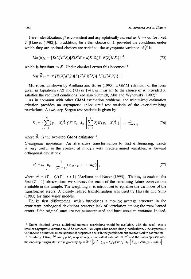
Given identification, fi is consistent and asymptotically normal as N oo for fixedT lHansen ( 1982)l In addition, for either choice of A, provided the conditions underwhich they are optimal choices are satisfied, the asymptotic variance of i is
Var(/3)R = {E(Xi'K'Zi)lE(Z'Kui ul K'Zi)l-E(Zi'K Xi)}- , ( 75)
which is invariant to K Under classical errors this becomes 14
Var( 13)c = o 2 {E(Xi'K'Z)lE(Z'KK'Zi)l I'E(Zli K Xi)}-'.
Moreover, as shown by Arellano and Bover ( 1995), a GMM estimator of the formgiven in Equations ( 72) and ( 73) or ( 74), is invariant to the choice of K provided Ksatisfies the required conditions lsee also Schmidt, Ahn and Wyhowski ( 1992)l.
As in common with other GMM estimation problems, the minimized estimationcriterion provides an asymptotic chi-squared test statistic of the overidentifyingrestrictions A two-step Sargan test statistic is given by
SR l (Yi -Xi R)'K'Zij AR ZK(Yi -Xi XR)l (q-k) ( 76)
where /i R is the two-step GMM estimator 15.
Orthogonal deviations An alternative transformation to first differencing, whichis very useful in the context of models with predetermined variables, is forwardorthogonal deviations:
= li u (T t)(Ui(t+ ) + T'"i)l , ( 77)
where c 2 = (T t)/(T t + 1) lArellano and Bover ( 1995)l That is, to each of thefirst (T 1) observations we subtract the mean of the remaining future observationsavailable in the sample The weighting c, is introduced to equalize the variances of thetransformed errors A closely related transformation was used by Hayashi and Sims( 1983) for time series models.
Unlike first differencing, which introduces a moving average structure in theerror term, orthogonal deviations preserve lack of correlation among the transformederrors if the original ones are not autocorrelated and have constant variance Indeed,
14 Under classical errors, additional moment restrictions would be available, with the result that a
smaller asymptotic variance could be achieved The expression above simply particularizes the asymptotic
variance to a situation where additional properties occur in the population but are not used in estimation.
15 Similarly, letting & 2 and tic be, respectively, a consistent estimate of a 2 and the one-step estimator,
the one-step Sargan statistic is given by Sc = a-2 lEN= ,(yi -Xifc)'K'Zl Ac lh i ZK(Yi -Xic)l.
3256
Ch 53: Panel Data Models Some Recent Developments
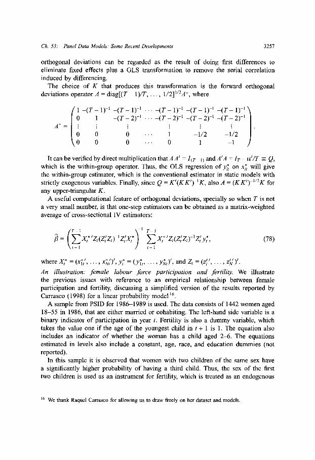
orthogonal deviations can be regarded as the result of doing first differences toeliminate fixed effects plus a GLS transformation to remove the serial correlationinduced by differencing.
The choice of K that produces this transformation is the forward orthogonaldeviations operator A = diagl(T )/T, , 1/2 l 1/ 2A+, where
I -(T I)-' -(T I -(T I) 1 -(T )-' -(T I) 0 1 -(T 2)-1 -(T 2)- 1 -(T 2) (T 2)- l
A+ = i 0 O O · · · 1 -1/2 -1/20 O O O 1 -1
It can be verified by direct multiplication that AA' = I(T I) and A'A = IT t'/T = which is the within-group operator Thus, the OLS regression of yi on x*t will givethe within-group estimator, which is the conventional estimator in static models withstrictly exogenous variables Finally, since Q = K'(KK') K, also A = (KK')-I/2 K forany upper-triangular K.
A useful computational feature of orthogonal deviations, specially so when T is nota very small number, is that one-step estimators can be obtained as a matrix-weightedaverage of cross-sectional IV estimators:
= (t E Xt Zt(Z Zt) IZX*t ) EX*'z(zz)-I' yt*, ( 78)
where X,* = (x*', , x J)', y* = (y*, , y nz)', and Z, = (z', ,
An illustration: female labour force participation and fertility We illustratethe previous issues with reference to an empirical relationship between femaleparticipation and fertility, discussing a simplified version of the results reported byCarrasco ( 1998) for a linear probability model 16
A sample from PSID for 1986-1989 is used The data consists of 1442 women aged18-55 in 1986, that are either married or cohabiting The left-hand side variable is abinary indicator of participation in year t Fertility is also a dummy variable, whichtakes the value one if the age of the youngest child in t + 1 is 1 The equation alsoincludes an indicator of whether the woman has a child aged 2-6 The equationsestimated in levels also include a constant, age, race, and education dummies (notreported).
In this sample it is observed that women with two children of the same sex havea significantly higher probability of having a third child Thus, the sex of the firsttwo children is used as an instrument for fertility, which is treated as an endogenous
16 We thank Raquel Carrasco for allowing us to draw freely on her dataset and models.
3257
M Arellano and B Honored
Table 2Linear probability models of female labour force participation ab (N = 1442, 1986-1989)
Variable OLS 2 SLSC WITHIN GM Md GM Me
Fertility -0 15 -1 01 -0 06 -0 08 -0 13
( 8.2) ( 2 1) ( 3 8) ( 2 8) ( 2 2)
Kids 2-6 -0 08 -0 24 0 001 -0 005 -0 09
( 5.2) ( 2 6) ( 0 04) ( 0 4) ( 2 7)
Sargan test 48 0 ( 22) 18 0 ( 10)
ml 19 0 5 7 -10 0 -10 0 -10 0
m 2 16 0 12 0 -1 7 -1 7 -1 6
Models including lagged participation
Fertility -0 09 -0 33 -0 06 -0 09 -0 14
( 5.2) ( 1 3) ( 3 7) ( 3 1) ( 2 2)
Kids 2-6 -0 02 -0 07 -0 000 -0 02 -0 10
( 2.1) ( 1 3) ( 0 00) ( 1 1) ( 3 5)
Lagged participation 0 63 0 61 0 03 0 36 0 29
( 42 0) ( 30 0) ( 1 7) ( 8 3) ( 6 3)
Sargan 51 0 ( 27) 25 0 ( 15)
ml -7 0 -5 4 -13 0 -14 0 -13 0
m 2 3 1 2 8 -1 3 1 5 1 2
a Heteroskedasticity robust t-ratios shown in parentheses.b GMM I Vs in bottom panel also include lags of participation up to t 2.'External instrument: previous children of same sex.d I Vs: all lags and leads of "kids 2-6 " and "same sex" variables (strictly exogenous).e I Vs: lags of "kids 2-6 " and "same sex" up to t (predetermined).
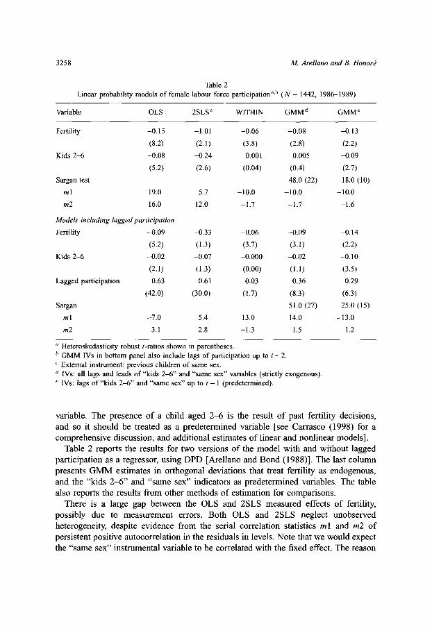
variable The presence of a child aged 2-6 is the result of past fertility decisions,and so it should be treated as a predetermined variable lsee Carrasco ( 1998) for acomprehensive discussion, and additional estimates of linear and nonlinear modelsl.
Table 2 reports the results for two versions of the model with and without laggedparticipation as a regressor, using DPD lArellano and Bond ( 1988)l The last columnpresents GMM estimates in orthogonal deviations that treat fertility as endogenous,and the "kids 2-6 " and "same sex" indicators as predetermined variables The tablealso reports the results from other methods of estimation for comparisons.
There is a large gap between the OLS and 2 SLS measured effects of fertility,possibly due to measurement errors Both OLS and 2 SLS neglect unobservedheterogeneity, despite evidence from the serial correlation statistics ml and m 2 ofpersistent positive autocorrelation in the residuals in levels Note that we would expectthe "same sex" instrumental variable to be correlated with the fixed effect The reason
3258
Ch 53: Panel Data Models: Some Recent Developments
is that it will be a predictor of preferences for children, given that the sample includeswomen with less than two children.
The within-groups estimator controls for unobserved heterogeneity, but in doingso we would expect it to introduce biases due to lack of strict exogeneity of theexplanatory variables The GMM estimates in column 4 deal with the endogeneity offertility and control for fixed effects, but treat the "kids 2-6 " and "same sex" variablesas strictly exogenous This results in a smaller effect of fertility on participation(in absolute value) than the one obtained in column 5 treating the variables aspredetermined The hypothesis of strict exogeneity of these two variables is rejectedat the 5 percent level from the difference in the Sargan statistics in both panels.(Both GMM estimates are "one-step", but all test statistics reported are robust toheteroskedasticity )
Finally, note that the ml and m 2 statistics (which are asymptotically distributed asa N(O, 1) under the null of no autocorrelation) have been calculated from residuals infirst differences for the within-groups and GMM estimates So if the errors in levelswere uncorrelated, we would expect ml to be significant, but not m 2, as is the casehere lcf , Arellano and Bond ( 1991)l.
Levels and differences estimators The GMM estimator proposed by Arellano andBover ( 1995) combined the basic moments ( 71) with E(Azi,ui,) = O (t = 2, , T).Using their notation, the full set of orthogonality conditions can be written in compactform as
E(Z+'Hui) = 0, ( 79)
where Zi+ is a block diagonal matrix with blocks Zi as above, and Zfi = diag (Az'2,. Az) H is the 2 (T 1) x T selection matrix H = (K',I')', where I, = ( IT ).
With these changes in notation, the form of the estimator is similar to that inEquation ( 72).
As before, a robust choice of A is provided by the inverse of an unrestrictedestimate of the variance matrix of the moments N 1 i, I Zi H uii i'H'Zi However,this can be a poor estimate of the population moments if N is not sufficiently largerelative to T, which may have an adverse effect on the finite sample properties ofthe GMM estimator Unfortunately, in this case an efficient one-step estimator underrestrictive assumptions does not exist Intuitively, since some of the instruments forthe equations in levels are not valid for those in differences, and conversely, not allthe covariance terms between the two sets of moments will be zero.
3.2 Efficient estimation under conditional mean independence
If lack of correlation between it and zit is replaced by an assumption of conditionalindependence in mean E(vi, I z) = 0, the model implies additional orthogonalityrestrictions This is so because it will be uncorrelated not only with the conditioning
3259
M Arellano and B Honored
variables zt but also with functions of them Chamberlain ( 1992 b) derived the semi-parametric efficiency bound for this model Hahn ( 1997) showed that a GMM estimatorbased on an increasing set of instruments as N tends to infinity would achieve thesemiparametric efficiency bound Hahn discussed the rate of growth of the number ofinstruments for the case of Fourier series and polynomial series.
Note that the asymptotic bound for the model based on E(voi, I z) = O will be ingeneral different from that of E(voi, z, /i) = 0, whose implications for linear projectionswere discussed in the previous section.
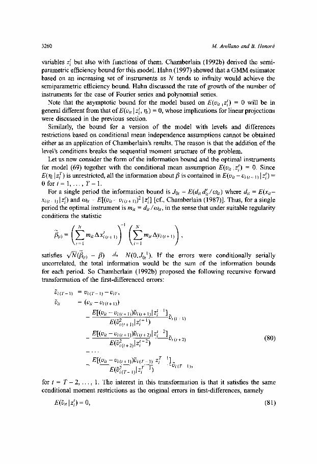
Similarly, the bound for a version of the model with levels and differencesrestrictions based on conditional mean independence assumptions cannot be obtainedeither as an application of Chamberlain's results The reason is that the addition of thelevel's conditions breaks the sequential moment structure of the problem.
Let us now consider the form of the information bound and the optimal instrumentsfor model ( 69) together with the conditional mean assumption E(voi, I z) = O SinceE(zf IZT) is unrestricted, all the information about /3 is contained in E(vi, vi (t + 1) lz I) =fort= 1, , T-1.
For a single period the information bound is Jot = E(dit dt/it) where d, = E(xit-xi (+ ) l 1 z) and oit = El(voi Vi(t+ 1)) zl lcf , Chamberlain ( 1987)l Thus, for a singleperiod the optimal instrument is mi, = di /it,, in the sense that under suitable regularityconditions the statistic
(t) ( mit Ax;(,+l) (m it Ayi(t+ 1)
satisfies v(( (t ( 3) A N(O,Jotl) If the errors were conditionally seriallyuncorrelated, the total information would be the sum of the information boundsfor each period So Chamberlain ( 1992 b) proposed the following recursive forwardtransformation of the first-differenced errors:
Di(T ) = Vi(T I)-U Vi T,
bit = (Vit -i(t+ 1))
El(vit vi(t+ 1))vi(+ 1)I Zi+ 1 lE(v ( + 1) v 1 (t+l)
El(it i(,t+l ))i(t+ 2)i l( 80)+)2 t+ 2 i(t+ 2) ( 80)
El(vit i(t+ ))Vi(T )z I Z l E(D 2 T I) i(T I),
for t = T 2, , 1 The interest in this transformation is that it satisfies the sameconditional moment restrictions as the original errors in first-differences, namely
3260
E(bi I t)= , ( 81)
Ch 53: Panel Data Models: Some Recent Developments
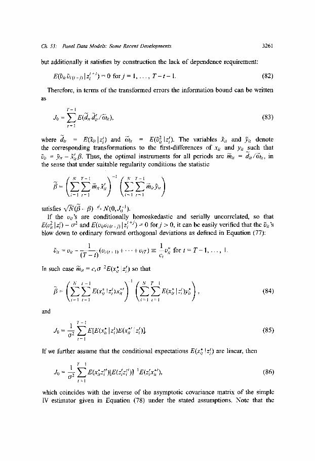
but additionally it satisfies by construction the lack of dependence requirement:
E(itjbi(t,+j) I z' + ) = O forj = 1, , T-t 1 ( 82)
Therefore, in terms of the transformed errors the information bound can be writtenas
T-I
Jo= ZE( d,td',/)J,), ( 83)t=l
where dit = E(,t I z') and wjit = E(D 2 I z) The variables Xi, and Pit denotethe corresponding transformations to the first-differences of xit and yit such thatbit = i x'13 Thus, the optimal instruments for all periods are mi, = dit/w i,, inthe sense that under suitable regularity conditions the statistic
N T-1 I N T-1
\i=l t=l i=l t=l
satisfies v N(j fi) d N(, Jol).If the v's are conditionally homoskedastic and serially uncorrelated, so that
E(v 2 I zi) = c 2and E(vivi(t+j) z>+) = O forj > O, it can be easily verified that the vi,'sblow down to ordinary forward orthogonal deviations as defined in Equation ( 77):
1 1it = O Ui (t)(i(t+l)+ +Ui T) = l*t fort= T-1, , 1.
(T t) Ct
In such case rit = c,a-2 E(xt* Izi) so that
13 = (i i E(x* z',*xw) (Z ZE(x Iz -ix)Y,*) ( 84)i=l t= l i=l t=l
and
1 T-Jo= z ElE(x* Iz)E(*'l)l ( 85)
t=l
If we further assume that the conditional expectations E(x* I z) are linear, then
T I
J= 2 E(x,*zi)lE(z'z Y)l-E(zix*') ( 86)t=l
which coincides with the inverse of the asymptotic covariance matrix of the simpleIV estimator given in Equation ( 78) under the stated assumptions Note that the
3261

M Arellano and B Honored
assumptions of conditional homoskedasticity, lack of serial correlation, and linearityof E(x* l z 1) would imply further conditional moment restrictions that may lower theinformation bound for / Here, we merely particularize the bound for /3 based onE(vit Izi) = O to the case where the additional restrictions happen to occur in thepopulation but are not used in the calculation of the bound.
3.3 Finite sample properties of GMM and alternative estimators
For sufficiently large N, the sampling distribution of the GMM estimators discussedabove can be approximated by a normal distribution However, the quality of theapproximation for a given sample size may vary greatly depending on the qualityof the instruments used Since the number of instruments increases with T, manyoveridentifying restrictions tend to be available even for moderate values of T, althoughthe quality of these instruments is often poor.
Monte Carlo results on the finite sample properties of GMM estimators for paneldata models with predetermined variables have been reported by Arellano and Bond( 1991), Kiviet ( 1995), Ziliak ( 1997), Blundell and Bond ( 1998) and Alonso-Borregoand Arellano ( 1999), amongst others A conclusion in common to these studies is thatGMM estimators that use the full set of moments available for errors in first-differencescan be severely biased, specially when the instruments are weak and the number ofmoments is large relative to the cross-sectional sample size.
From the literature on the finite sample properties of simultaneous equationsestimators, we know that the effect of weak instruments on the distributions of 25 LSand LIML differs substantially, in spite of the fact that both estimators have thesame asymptotic distribution While LIML is approximately median unbiased, 25 LSis biased towards OLS, and in the case of lack of identification in the population itconverges to a random variable with the OLS probability limit as its central value.In contrast, LIML has no moments, and as a result its distribution has thicker tailsthan that of 2 SLS and a higher probability of outliers lcf , Phillips ( 1983)l Anderson,Kunitomo and Sawa ( 1982) carried out numerical comparisons of the distributions ofthe two estimators, and concluded that LIML was to be strongly preferred to 25 LS,specially in cases with a large number of instruments.
LIML analogue estimators It is thus of interest to consider LIML analogues for ourmodels, and compare their finite sample properties with those of GMM estimators.Following Alonso-Borrego and Arellano ( 1999), a non-robust LIML analogue PLIMLI
minimizes a criterion of the form
= (y* -X*/3)M(y* -X*'/3)ec(/3) =(y _X /3)f By _ /3), ( 87)
where starred variables denote orthogonal deviations, y* = (y*', , y/)', X* = (XI*'
. , XN')', Z = (Zr, , ZN)', and M = Z(Z'Z)' Z' The resulting estimator is
OLIMLI = (X*'MX* X*X * ) (X* My* -X'y*),
3262
( 88)
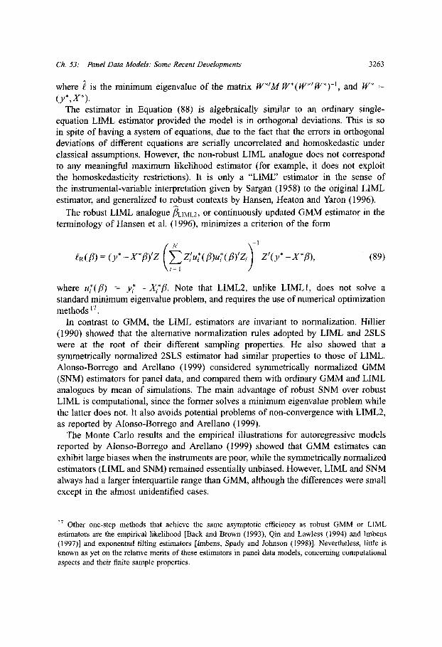
Ch 53: Panel Data Models: Some Recent Developments
where is the minimum eigenvalue of the matrix W*'M W*(W*'W*) - l, and W* =
(y*,X*).The estimator in Equation ( 88) is algebraically similar to an ordinary single-
equation LIML estimator provided the model is in orthogonal deviations This is soin spite of having a system of equations, due to the fact that the errors in orthogonaldeviations of different equations are serially uncorrelated and homoskedastic underclassical assumptions However, the non-robust LIML analogue does not correspondto any meaningful maximum likelihood estimator (for example, it does not exploitthe homoskedasticity restrictions) It is only a "LIME' estimator in the sense ofthe instrumental-variable interpretation given by Sargan ( 1958) to the original LIMLestimator, and generalized to robust contexts by Hansen, Heaton and Yaron ( 1996).
The robust LIML analogue LIML 2, or continuously updated GMM estimator in theterminology of Hansen et al ( 1996), minimizes a criterion of the form
GR(/i) = (Y -X i)Z u(fi)u*(i 3)'Z ZI(y* -X 3), ( 89)
where u*(f) = y Xi*f Note that LIML 2, unlike LIMLI, does not solve astandard minimum eigenvalue problem, and requires the use of numerical optimizationmethods 17
In contrast to GMM, the LIML estimators are invariant to normalization Hillier( 1990) showed that the alternative normalization rules adopted by LIML and 25 LSwere at the root of their different sampling properties He also showed that asymmetrically normalized 2 SLS estimator had similar properties to those of LIML.Alonso-Borrego and Arellano ( 1999) considered symmetrically normalized GMM(SNM) estimators for panel data, and compared them with ordinary GMM and LIMLanalogues by mean of simulations The main advantage of robust SNM over robustLIML is computational, since the former solves a minimum eigenvalue problem whilethe latter does not It also avoids potential problems of non-convergence with LIML 2,as reported by Alonso-Borrego and Arellano ( 1999).
The Monte Carlo results and the empirical illustrations for autoregressive modelsreported by Alonso-Borrego and Arellano ( 1999) showed that GMM estimates canexhibit large biases when the instruments are poor, while the symmetrically normalizedestimators (LIML and SNM) remained essentially unbiased However, LIML and SNMalways had a larger interquartile range than GMM, although the differences were smallexcept in the almost unidentified cases.
17 Other one-step methods that achieve the same asymptotic efficiency as robust GMM or LIMLestimators are the empirical likelihood lBack and Brown ( 1993), Qin and Lawless ( 1994) and Imbens( 1997)l and exponential tilting estimators lImbens, Spady and Johnson ( 1998)l Nevertheless, little isknown as yet on the relative merits of these estimators in panel data models, concerning computationalaspects and their finite sample properties.
3263
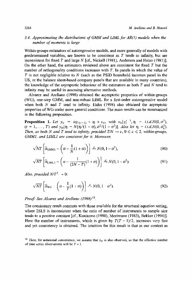
M Arellano and B Honors
3.4 Approximating the distributions of GMM and LIML for AR() models when thenumber of moments is large
Within-groups estimators of autoregressive models, and more generally of models withpredetermined variables, are known to be consistent as T tends to infinity, but areinconsistent for fixed T and large N lcf , Nickell ( 1981), Anderson and Hsiao ( 1981)l.On the other hand, the estimators reviewed above are consistent for fixed T but thenumber of orthogonality conditions increases with T In panels in which the value ofT is not negligible relative to N (such as the PSID household incomes panel in theUS, or the balance sheet-based company panels that are available in many countries),the knowledge of the asymptotic behaviour of the estimators as both T and N tend toinfinity may be useful in assessing alternative methods.
Alvarez and Arellano ( 1998) obtained the asymptotic properties of within-groups(WG), one-step GMM, and non-robust LIML for a first-order autoregressive modelwhen both N and T tend to infinity Hahn ( 1998) also obtained the asymptoticproperties of WG under more general conditions The main results can be summarizedin the following proposition.
Proposition 1 Let it = ayi(t 1) + ri + vi,, with vitly ,rri ~ i i d N(O, a 2 ),(t = 1, , T) and Yio Oli ~ Nlhj/( 1 a), a 2 /( 1 a 2)l Also let rih i i d N(O, r 2).Then, as both N and T tend to infinity, provided T/N c, O < c < 2, within-groups,GMM 1, and LIML 1 are consistent for a Moreover,
T lMM (a-N( 1 + a))l A N(O, -a 2 ), ( 90)
NT la LIMLI (a ( 2 N T)( 1 + a)) d• 4 N(O, 1 a 2 ) ( 91)
Also, provided N/T 3 0:
T law G (a (l + a))l 4 N(O, 1 a 2 ) ( 92)
Proof: See Alvarez and Arellano ( 1998) 18
The consistency result contrasts with those available for the structural equation setting,where 2 SLS is inconsistent when the ratio of number of instruments to sample sizetends to a positive constant lcf , Kunitomo ( 1980), Morimune ( 1983), Bekker ( 1994)l.Here the number of instruments, which is given by T(T 1)/2, increases very fastand yet consistency is obtained The intuition for this result is that in our context as
18 Here, for notational convenience, we assume that Yio is also observed, so that the effective numberof time series observations will be T + 1.
3264
Ch 53: Panel Data Models: Some Recent Developments
T tends to infinity the "simultaneity bias" tends to zero, and so closeness of GMM 1or LIML 1 to OLS in orthogonal deviations (ie within-groups) becomes a desirableproperty.
Note that when T/N o O the fixed T results for GMM 1 and LIML 1 remainvalid, but within-groups, although consistent, has an asymptotic bias in its asymptoticdistribution (which would only disappear if N/T 0) However, when T/N tends to apositive constant, within-groups, GMM 1 and LIML 1 exhibit negative biases in theirasymptotic distributions The condition that c > 2 is not restrictive since GMM 1 andLIML 1 are only well defined for (T 1)/N < 1 Thus, for T < N the GMM 1 bias isalways smaller than the within-groups bias, and the LIML 1 bias is smaller than theother two.
Another interesting feature is that the three estimators are asymptotically efficient inthe sense of attaining the same asymptotic variance as the within-groups estimator asT x oc However, Alvarez and Arellano ( 1998) show that the standard formulae forfixed T estimated variances of GMM 1 and LIML 1, which depend on the variance ofthe fixed effect, remain consistent estimates of the asymptotic variances as T oo.
These results provide some theoretical support for LIML 1 over GMM 1 They alsoillustrate the usefulness of understanding the properties of panel data estimators asthe time series information accumulates, even for moderate values of T: in a fixedT framework, GMM 1 and LIML 1 are asymptotically equivalent, but as T increasesLIML 1 has a smaller asymptotic bias than GMM 1.
The crude GMM estimator in first differences Alvarez and Arellano ( 1998) also showthat the crude GMM estimator (CIV) that neglects the autocorrelation in the firstdifferenced errors (ie , one-step GMM in first-differences with weight matrix equalto (Z'Z)-1) is inconsistent as T/N c > 0, despite being consistent for fixed T Theresult is:
taclv f a 2 ( 1 + ( 2 -2 c)( 93)2)
The intuition for this result is that the "simultaneity bias" of OLS in first differences(unlike the one for orthogonal deviations) does not tend to zero as T oo.Thus, for fixed T the IV estimators in orthogonal deviations and first differencesare both consistent, whereas as T increases the former remains consistent but thelatter is inconsistent Moreover, notice that the bias may be qualitatively relevant.Standard fixed-T large-N GMM theory would just describe the CIV estimator as beingasymptotically less efficient than GMM 1 as a consequence of using a non-optimalchoice of weighting matrix.
4 Nonlinear panel data models
The ability to difference out the individual specific effect as was done in the previoussections relies heavily on the linear or multiplicative way in which it entered the model.
3265
M Arellano and B Honors
Many simple cross sectional models have a constant that does not enter in this way.This is for example true for all the limited dependent variable models discussed inChapters 9 and 10 of Amemiya ( 1985) Introducing an individual specific effect as anindividual specific constant in those models therefore results in models that cannot beestimated by the methods discussed so far As will be seen in the following sections,the currently available methods for dealing with these models, rely on insights thatare model-specific and that do not always seem to be useful for similar, but slightlydifferent models The main exception to this is the conditional maximum likelihoodapproach which has been used to construct estimators for some exponential familymodels We discuss this method in the next section.
Unfortunately, there are many models for which it is not possible to use theconditional likelihood approach to eliminate the individual specific effect For some ofthose models, alternative appoaches have been developed In Sections 6 and 7, we willreview some of the progress that has been made in the area of estimation of limiteddependent variable models with individual-specific, "fixed", effects 19 This literatureis closely related to the literature that deals with estimation of semiparametric limiteddependent variables models, in that it is usually not necessary to specify a parametricform for the distribution of the underlying errors The models are also semiparametricin the sense that the distribution of the individual specific effects conditional on theexplanatory variable, is left unspecified It is therefore not surprising that there is aclose relationship between some of the approaches that are discussed here, and someapproaches that have been taken to estimation of semiparametric limited dependentvariables models Indeed, in some cases the estimators for the panel data models havepreceded the "corresponding" estimators for the cross sectional models.
The main limitation of much of the literature on nonlinear panel data methods, is thatit is assumed that the explanatory variables are strictly exogenous in the sense that someassumptions will be made on the errors conditional on all (including future) valuesof the explanatory variables As was pointed out earlier in this chapter, many of therecent advances in estimation of linear panel data models have focused on relaxing thisassumption In Section 8, we will discuss how some of the methods can be generalizedto allow for lagged dependent variables, but at this point very little is known aboutestimation of nonlinear panel data models with predetermined explanatory variables.
The discussion of nonlinear panel data models in the next three sections will focusentirely on standard nonlinear econometric models in which the parameter that isusually interpreted as an intercept, is allowed to be individual specific This seemslike a natural first step in understanding the value and limitations of panel data whenthe model of interest is nonlinear However, it is clear that knowing the "parameters
19 Even though one often imagines a random sample of individuals, and hence random draws of theindividual specific effects, it is customary to call the effect "fixed" when no assumptions are made onits relationship with other explanatory variables A random effect is one which has been modelled insome manner.
3266
Ch 53: Panel Data Models: Some Recent Developments
of interest" in the models discussed below does not always allow one to infer all thequantities of interest For example, in the fixed effects logit model below, knowing/3 will not allow one to infer the effect of one of the explanatory variables on theprobability distribution of the dependent variable, although knowing the vector of O 3 'swill allow one to infer the relative effects of the explanatory variables This problem isdue to the semiparametric nature of the nonlinear models considered here, and is notparticular to panel data On the other hand, if the censoring in Equation ( 103) belowis due to top or bottom coding of the true dependent variable of interest, then theinterpretation of the parameters of the censored regression model is exactly the sameas the interpretation of the parameters of a linear panel data model The same cansometimes be said for the selection models discussed below.
Another limitation of most of the discussion here is that it focuses on the extremecase where no assumptions are made on the relationship between the individual specificeffect and the explanatory variables Whether a more "random" effects approach wheresome assumptions are made on how the distribution of this effect depends on theexplanatory variables is more useful, depends on the context (and one's taste) Insection 9 we briefly discuss some recent advances in this area We devote much lessspace to that topic because many of the new developments there are by-productsof developments in other areas of econometrics For example, recent developmentsin Bayesian econometrics and in simulation-based inference have implications fornonlinear random effects panel data models, but the main new insights are moregeneral, and not really tied to panel data.
5 Conditional maximum likelihood estimation
In a static linear model, one can justify treating the individual specific effects asparameters to be estimated by reference to the Frisch-Waugh Theorem: OLS (ornormal maximum likelihood) on individual specific dummy variables is numericallyequivalent to OLS on deviations from means This means that including individualspecific dummies yields a consistent estimator of the slope parameters (as N goes toinfinity), even though the number of parameters is also going to infinity Unfortunately,as was pointed in the classic paper by Neyman and Scott ( 1948), it is generally not thecase that the maximum likelihood estimator will retain its nice asymptotic propertieswhen the number of parameters is allowed to increase with sample size This is forexample seen by considering the maximum likelihood estimator of the variance in astatic linear panel data model with normal errors: because the maximum likelihoodestimator does not make the degrees-of-freedom correction, it will be inconsistent ifthe number of parameters is of order n.
Conditional maximum likelihood estimation is a method which, when it isapplicable, can be used to construct consistent estimators of panel data models in thepresence of individual specific effects The idea is as follows Suppose that a randomvariable, yi,, has distribution f ( ; 0, a') where O is the parameter of interest and is
3267
M Arellano and B Honored
common for all i, whereas ai is a nuisance parameter which is allowed to differ across i.A sufficient statistic, Ti, for ai is a function of the data such that the distribution ofthe data given T does not depend on ai However, it might well depend on O If thatis the case, then one can estimate O by maximum likelihood using the conditionaldistribution of the data given the sufficient statistics Andersen ( 1970) proved that theresulting estimator is consistent and asymptotically normal under appropriate regularityconditions In the two subsections below, we give examples of how the conditionalmaximum likelihood estimator can be used to construct estimators of the panel datalogit and the panel data Poisson regression models.
The problem with conditional maximum likelihood estimation as a general prescrip-tion for constructing estimators of nonlinear panel data models is that it is not alwayspossible to find sufficient statistics such that the conditional distribution of the dataconditional on the sufficient statistic will depend on O This is the case for many ofthe nonlinear models used in econometrics.
5.1 Conditional maximum likelihood estimation of logit models
The simplest interesting nonlinear model for which the conditional likelihood approachworks, is the "textbook" logit model studied in Rasch ( 1960, 1961) With two timeperiods and an individual specific constant we have,
Yit = 1 {xit/3, + a + eit 0) t = 1,2, i = 1, , n
where et and i 2 are independent and logistically distributed, conditional on ai, Xil, x 2.It follows that
Pr(yit = llxil,Xi 2, ai)= exp(xit/3 + ai) ( 94)1 + exp (xit/ + a ( 4
In this case it is easy to see how the conditional likelihood approach "eliminates"the individual specific effect Define events A and B by A = {yin = 0, Yi 2 = 1 } andB = { yil = 1, yi 2 = O } It is then an easy exercise to show that
Pr (il = O,Yi 2 = Yil +Yi 2 = ,xil,xi 2, ai) = Pr (A A U B,xil,xi 2 ,ai)
~~ 1 = I, ( 95)1 + exp ((Xil -Xi 2) '
In words, if we restrict the sample to the observations for which yit changes, then theindividual specific effects do not enter the distribution of (Yil,Yi 2) given (xil ,Xi 2 , ai)and the distribution of yil given (xil, Xi 2) has the form of a logit model with explanatoryvariable xil Xi 2 and coefficient /3 Intuitively, the implication is that if we restrict thesample to the observations for which yi, changes over time, then / can be estimatedby estimating a logit in the restricted sample without having to specify the distribution
3268
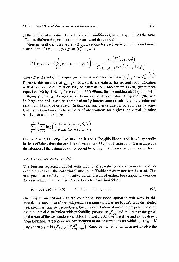
Ch 53 Panel Data Models: Some Recent Developments
of the individual specific effects In a sense, conditioning on yi I +Yi 2 = 1 has the sameeffect as differencing the data in a linear panel data model.
More generally, if there are T > 2 observations for each individual, the conditionaldistribution of (yi, yi,) given Et= ,yit is
P Yil, Yit E Yit Xil, , it, i T T
(d, d,)CB exp (,t I d x itf )( 96)
where B is the set of all sequences of zeros and ones that have tt d/ = ,T o yit.
Formally this means that T= I it is a sufficient statistic for ai, and the implicationis that one can use Equation ( 96) to estimate B Chamberlain ( 1980) generalizedEquation ( 96) by deriving the conditional likelihood for the multinomial logit model.
When T is large, the number of terms in the denominator of Equation ( 96) willbe large, and and it can be computationally burdensome to calculate the conditionalmaximum likelihood estimator In that case one can estimate fl by applying the logicleading to Equation ( 95) to all pairs of observations for a given individual In otherwords, one can maximize
E exp (yit (xi, xi S,) )Ei= log 1 +exp((xit, -x J),) '
Unless T = 2, this objective function is not a (log-)likelihood, and it will generallybe less efficient than the conditional maximum likelihood estimator The asymptoticdistribution of the estimator can be found by noting that it is an extremum estimator.
5.2 Poisson regression models
The Poisson regression model with individual specific constants provides anotherexample in which the conditional maximum likelihood estimator can be used Thisis a special case of the multiplicative model discussed earlier For simplicity, considerthe case where there are two observations for each individual:
yit po (exp(ai + xit)) t = 1,2 i = 1, , n ( 97)
One way to understand why the conditional likelihood approach will work in thismodel, is to recall that if two independent random variables are both Poisson distributedwith means ul and bt 2, respectively, then the distribution of one of them given the sum,has a binomial distribution with probability parameter tl-' and trial parameter givenby the sum of the two random variables It therefore follows that ifyil andy/ 2 are drawnfrom Equation ( 97) and we restrict attention to the observations for which Yil + Yi 2 = K
(say), then yil bi (K, exp(x Si)-exp(x 2 ) Since this distribution does not involve the(say),~~~~~~ ey Xi I bi K¢px)+ ¢XP(Xi 2 M)
3269
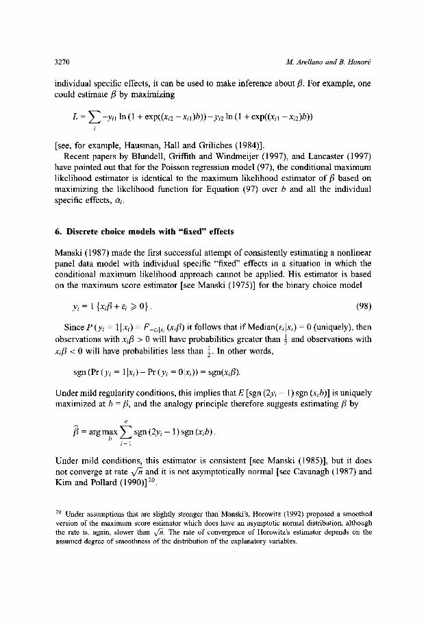
M Arellano and B Honor
individual specific effects, it can be used to make inference about f 3 For example, onecould estimate /3 by maximizing
L = -yil In ( 1 + exp((xi 2 xil)b)) -Yi 2 In ( 1 + exp((xi xi 2)b))
lsee, for example, Hausman, Hall and Griliches ( 1984)l.Recent papers by Blundell, Griffith and Windmeijer ( 1997), and Lancaster ( 1997)
have pointed out that for the Poisson regression model ( 97), the conditional maximumlikelihood estimator is identical to the maximum likelihood estimator of /3 based onmaximizing the likelihood function for Equation ( 97) over b and all the individualspecific effects, a.
6 Discrete choice models with "fixed" effects
Manski ( 1987) made the first successful attempt of consistently estimating a nonlinearpanel data model with individual specific "fixed" effects in a situation in which theconditional maximum likelihood approach cannot be applied His estimator is basedon the maximum score estimator lsee Manski ( 1975)l for the binary choice model
Yi = 1 xi/ + Ei > 0) ( 98)
Since P (yi = 1 I xi) = FE, lxi (xi,/) it follows that if Median(ei Ixi) = O (uniquely), thenobservations with xi/3 > O will have probabilities greater than and observations with2xi/ < O will have probabilities less than In other words,
sgn (Pr (i = 1 xi) Pr (i = O lxi)) = sgn(xii/).
Under mild regularity conditions, this implies that E lsgn ( 2 yi 1) sgn (xib)l is uniquelymaximized at b = /, and the analogy principle therefore suggests estimating /i by
n
/3 = arg max sgn ( 2 yi 1) sgn (xib).i=l
Under mild conditions, this estimator is consistent lsee Manski ( 1985)l, but it doesnot converge at rate /~ and it is not asymptotically normal lsee Cavanagh ( 1987) andKim and Pollard ( 1990)l 20.
20 Under assumptions that are slightly stronger than Manski's, Horowitz ( 1992) proposed a smoothedversion of the maximum score estimator which does have an asymptotic normal distribution, althoughthe rate is, again, slower than V/f The rate of convergence of Horowitz's estimator depends on theassumed degree of smoothness of the distribution of the explanatory variables.
3270
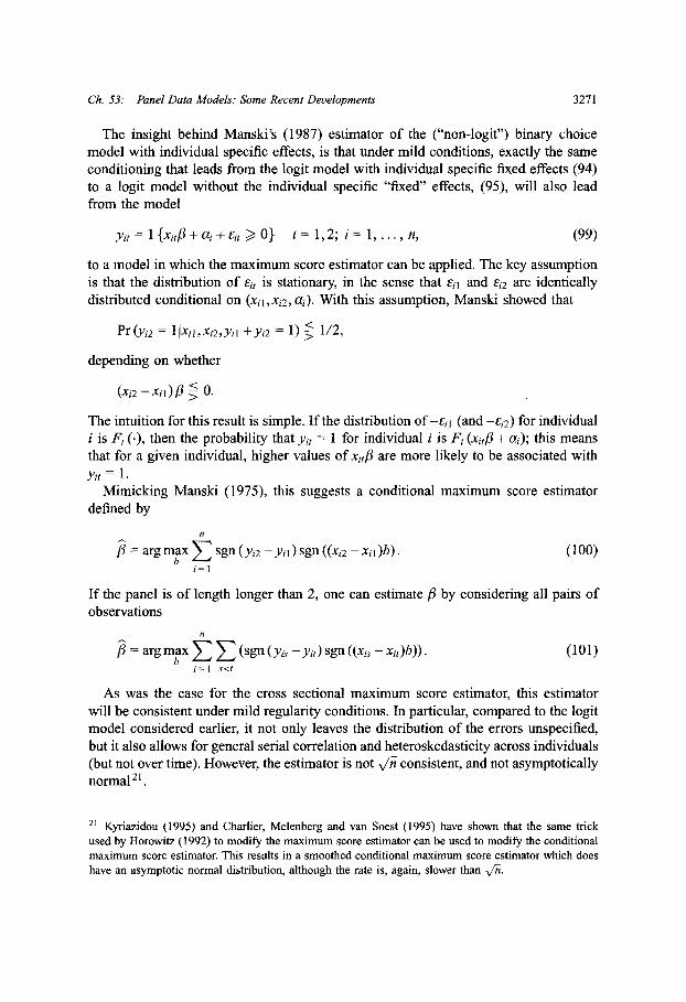
Ch 53: Panel Data Models: Some Recent Developments
The insight behind Manski's ( 1987) estimator of the ("non-logit") binary choicemodel with individual specific effects, is that under mild conditions, exactly the sameconditioning that leads from the logit model with individual specific fixed effects ( 94)to a logit model without the individual specific "fixed" effects, ( 95), will also leadfrom the model
Yit = 1 xit + ai + it O t = 1,2 ; i = 1 , n, ( 99)
to a model in which the maximum score estimator can be applied The key assumptionis that the distribution of ei, is stationary, in the sense that eil and Ei 2 are identicallydistributed conditional on (xil,xi 2, a,) With this assumption, Manski showed that
Pr (yi 2 = 1 j Xil,Xi 2,yi +Yi 2 = 1) 1/2,
depending on whether
(Xi 2 -Xil)# > 0.
The intuition for this result is simple If the distribution of -eil (and -Ei 2) for individuali is Fi ( ), then the probability that yit = 1 for individual i is F (xi,t + a,); this meansthat for a given individual, higher values of xit, are more likely to be associated withYit = 1.
Mimicking Manski ( 1975), this suggests a conditional maximum score estimatordefined by
n
3 = arg max sgn (Yi 2 -i ) sgn ((xi 2 xi )b) ( 100)
If the panel is of length longer than 2, one can estimate fi by considering all pairs ofobservations
, = argmax (sgn (y,s -yi) sgn ((x, -xit)b)) ( 101)i= st
As was the case for the cross sectional maximum score estimator, this estimatorwill be consistent under mild regularity conditions In particular, compared to the logitmodel considered earlier, it not only leaves the distribution of the errors unspecified,but it also allows for general serial correlation and heteroskedasticity across individuals(but not over time) However, the estimator is not +vr consistent, and not asymptoticallynormal 2.
21 Kyriazidou ( 1995) and Charlier, Melenberg and van Soest ( 1995) have shown that the same trickused by Horowitz ( 1992) to modify the maximum score estimator can be used to modify the conditionalmaximum score estimator This results in a smoothed conditional maximum score estimator which doeshave an asymptotic normal distribution, although the rate is, again, slower than /hn.
3271
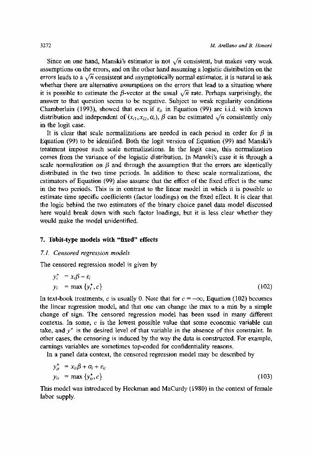
M Arellano and B Honors
Since on one hand, Manski's estimator is not /E consistent, but makes very weakassumptions on the errors, and on the other hand assuming a logistic distribution on theerrors leads to a v Fl consistent and asymptotically normal estimator, it is natural to askwhether there are alternative assumptions on the errors that lead to a situation whereit is possible to estimate the /3-vector at the usual /I rate Perhaps surprisingly, theanswer to that question seems to be negative Subject to weak regularity conditionsChamberlain ( 1993), showed that even if it in Equation ( 99) are i i d with knowndistribution and independent of (xil,xi 2, ai), /3 can be estimated /E consistently onlyin the logit case.
It is clear that scale normalizations are needed in each period in order for / inEquation ( 99) to be identified Both the logit version of Equation ( 99) and Manski'streatment impose such scale normalizations In the logit case, this normalizationcomes from the variance of the logistic distribution In Manski's case it is through ascale normalization on 3 and through the assumption that the errors are identicallydistributed in the two time periods In addition to these scale normalizations, theestimators of Equation ( 99) also assume that the effect of the fixed effect is the samein the two periods This is in contrast to the linear model in which it is possible toestimate time specific coefficients (factor loadings) on the fixed effect It is clear thatthe logic behind the two estimators of the binary choice panel data model discussedhere would break down with such factor loadings, but it is less clear whether theywould make the model unidentified.
7 Tobit-type models with "fixed" effects
7.1 Censored regression models
The censored regression model is given by
y? = xi + iyi = max {yi*, c} ( 102)
In text-book treatments, c is usually O Note that for c = -oc, Equation ( 102) becomesthe linear regression model, and that one can change the max to a min by a simplechange of sign The censored regression model has been used in many differentcontexts In some, c is the lowest possible value that some economic variable cantake, and y* is the desired level of that variable in the absence of this constraint Inother cases, the censoring is induced by the way the data is constructed For example,earnings variables are sometimes top-coded for confidentiality reasons.
In a panel data context, the censored regression model may be described by
yit = xi + ai + Eit
Yit = max {yt, c} ( 103)
This model was introduced by Heckman and Ma Curdy ( 1980) in the context of femalelabor supply.
3272
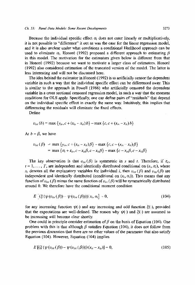
Ch 53: Panel Data Models: Some Recent Developments
Because the individual specific effect ai does not enter linearly or multiplicatively,it is not possible to "difference" it out as was the case for the linear regression model,and it is also unclear under what conditions a conditional likelihood approach can beused to eliminate ai Honor ( 1992) proposed a different approach to estimating /3in this model The motivation for the estimators given below is different from thatin Honors ( 1992) because we want to motivate a larger class of estimators Honor( 1992) also considered estimation of the truncated version of the model The latter isless interesting and will not be discussed here.
The idea behind the estimator in Honor 6 ( 1992) is to artificially censor the dependentvariable in such a way that the individual specific effect can be differenced away Thisis similar to the approach in Powell ( 1986) who artificially censored the dependentvariable in a cross sectional censored regression model, in such a way that the momentconditions for OLS apply Specifically, one can define pairs of "residuals" that dependon the individual specific effect in exactly the same way Intuitively, this implies thatdifferencing the residuals will eliminate the fixed effects.
Define
Uist (b) = max {yi,, c + (xi, xi,) b} max {c, c + (xi, xit) b}
At b = /, we have
oist (/3) = max {Yis, c + (xis xit) 3 } max {c, c + (xi, xit)/3 }= max {ai + Eis, c Xis 13, c xit 3 } max {c Xisf, c xit/3 }
The key observation is that visit (/3) is symmetric in S and t Therefore, if Eit,t = 1, , T, are independent and identically distributed conditional on (xi, ai), wherexi denotes all the explanatory variables for individual i, then vis (/3) and vit (/3) areindependent and identically distributed (conditional on (xi, ai)) This means that anyfunction of ois, (/3) minus the same function of vits (/3) will be symmetrically distributedaround O We therefore have the conditional moment condition
E l ( ( (its (/3) V (ist ()))1 xi, ail = 0, ( 104)
for any increasing function (-) and any increasing and odd function ~( ), providedthat the expectations are well-defined The reason why ip( ) and () are assumed tobe increasing will become clear shortly.
One could in principle consider estimation of /3 on the basis of Equation ( 104) Oneproblem with this is that although f satisfies Equation ( 104), it does not follow fromthe previous discussion that there are no other values of the parameter that also satisfyEquation ( 104) However, Equation ( 104) implies
E l( ( (vits (/3)) 4 (is t (/3)))) (xit xis)l = ,
3273
( 105)
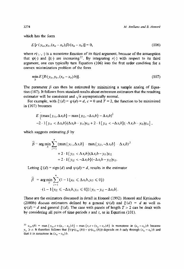
M Arellano and B Honors
which has the form
E lr (yis,Yit, (xi, xit) 8) (xis Xit)l = 0, ( 106)
where r( ,-, ) is a monotone function of its third argument, because of the assumptionthat p( ) and () are increasing 2 2 By integrating r() with respect to its thirdargument, one can typically turn Equation ( 106) into the first order condition for aconvex minimization problem of the form
min E lR (yi,,yi, (xis xit) b)l ( 107)b
The parameter P can then be estimated by minimizing a sample analog of Equa-tion ( 107) It follows from standard results about extremum estimators that the resultingestimator will be consistent and V/n asymptotically normal.
For example, with ~ (d)= p (d) = d, c = O and T = 2, the function to be minimizedin ( 107) becomes
E l(max{yil, Axib} max Yi 2, -Axib} Axb) 2
+ 2 l{ yil < Axib}(Axib -yil)yi 2 + 2 l{Yi 2 < -Axib}(-Axib -Yi 2)yil,
which suggests estimating /3 by
n
= arg min E (max{ yil , Axib} max Yi 2, -Axib} Axib) 2
i= 1
+ 2 l{Yil < Axib}(Axib -Yil)yi 2
+ 2 l{yi 2 < -Axib}(-Axib -Yi 2)Yil.
Letting ~ (d) = sign (d) and ip (d) = d, results in the estimator
n
/3 = argmin ( 1 I{yl < Axib,yi 2 O })i=l
( 1 {yi 2 < -Axib,yil < O }) l Yil -Yi 2 Axibl
These are the estimators discussed in detail in Honor 6 ( 1992) Honor and Kyriazidou( 2000 b) discuss estimators defined by a general i (d) and (d) = d as well asVp (d) = d and general 5 (d) The case with panels of length T > 2 can be dealt withby considering all pairs of time periods S and t, as in Equation ( 101).
22 Vit (b) = max {y,, c + (x xi )b} max {c, c + (xis -x, )b} is monotone in (xi, -x,,)b becauseyis > c It therefore follows that (' (ui, (b)) Vi (uist (b))) depends on b only through (xi, -xi,) b andthat it is monotone in (xi, -xi,)b.
3274
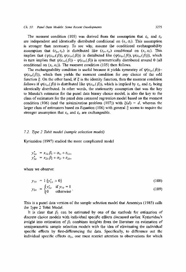
Ch 53: Panel Data Models: Some Recent Developments
The moment condition ( 105) was derived from the assumption that Eis and E,are independent and identically distributed conditional on (xi, a) This assumptionis stronger than necessary To see why, assume the conditional exchangeabilityassumption that (Es, eit) is distributed like (Eit,Eis) conditional on (xi, ai) Thisimplies that ((vjt(fi)), p(vi,s(f))) is distributed like (P(vits(f)), P(vist(/))), whichin turn implies that t(vs(fi)) P(vjts(i 3)) is symmetrically distributed around 0 (allconditional on (xi, as)) The moment condition ( 105) then follows.
The exchangeability condition is useful because it yields symmetry of t(vi,(i 3))-P(vtr(f)), which then yields the moment condition for any choice of the oddfunction A On the other hand, if ~ is the identity function, then the moment conditionfollows if (vis,( /)) is distributed like P(vijt,()), which is implied by Ei, and Eit beingidentically distributed In other words, the stationarity assumption that was the keyto Manski's estimator for the panel data binary choice model, is also the key to theclass of estimators for the panel data censored regression model based on the momentcondition ( 106) (and the minimization problem ( 107)) with (d) = d, whereas thelarger class of estimators based on Equation ( 106) with general ~ seems to require thestronger assumption that Ei, and Eit are exchangeable.
7.2 Type 2 Tobit model (sample selection model)
Kyriazidou ( 1997) studied the more complicated model
Yit = Xlit, 1 + ali + Elit,
Y 2 it = X 2 it 32 + a 2 i + E 2 it,
where we observe:
ylit = 1 {y*, > O } ( 108)
Y 2 it = i otherwise ( 109)
This is a panel data version of the sample selection model that Amemiya ( 1985) callsthe Type 2 Tobit Model.
It is clear that /3 l can be estimated by one of the methods for estimation ofdiscrete choice models with individual specific effects discussed earlier Kyriazidou'sinsight into estimation of /2 combines insights from the literature on estimation ofsemiparametric sample selection models with the idea of eliminating the individualspecific effects by first-differencing the data Specifically, to difference out theindividual specific effects a 2 i, one must restrict attention to observations for which
3275
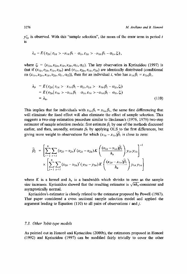
M Arellano and B Honor
Yit is observed With this "sample selection", the mean of the error term in period tis
Ait = E(E 2 itj Elit > -Xlit 3l li, Elis > -Xis Pl ali, ~i),
where i = (Xlis,X 2is,Xlit,x 2 it, ail, ai 2) The key observation in Kyriazidou ( 1997) isthat if (Elit, E 2 it, Elis, E 2 is) and (elis, E 2 is, Elit, e 2 i) are identically distributed (conditionalon (Xli,X 2 is,Xli,,x 2 it,, ail, ai 2)), then for an individual i, who has xli,f 31 = lisf 1,
Ait = E(E 2 it I Elit > -Xlit P 31 ali, Elis > -Xlisf 1i li, )
= E ( E 2 isl elis > -Xl is l li, Elit > -Xl it Pl li, i)
= Ais ( 110)
This implies that for individuals with xlit Pl = x i,/31, the same first differencing thatwill eliminate the fixed effect will also eliminate the effect of sample selection Thissuggests a two-step estimation procedure similar to Heckman's ( 1976, 1979) two-stepestimator of sample selection models: first estimate 1 by one of the methods discussedearlier, and then, secondly, estimate /32 by applying OLS to the first differences, butgiving more weight to observations for which (xli, -Xlj,)fl is close to zero:
/32 lE (X 2 it X 2 is) ( (it X 2 i (X 1 1 ) 1 Yit X Yiislis
X E"·"~ N ""( (Xit XlislflE (x 2 it -X 2 is) (Y 2 it -Y 2 is)K h Ylit Ylis
where K is a kernel and h, is a bandwidth which shrinks to zero as the samplesize increases Kyriazidou showed that the resulting estimator is n-consistent andasymptotically normal.
Kyriazidou's estimator is closely related to the estimator proposed by Powell ( 1987).That paper considered a cross sectional sample selection model and applied theargument leading to Equation ( 110) to all pairs of observations i and j.
7.3 Other Tobit-type models
As pointed out in Honor 6 and Kyriazidou ( 2000 b), the estimators proposed in Honor 6( 1992) and Kyriazidou ( 1997) can be modified fairly trivially to cover the other
3276
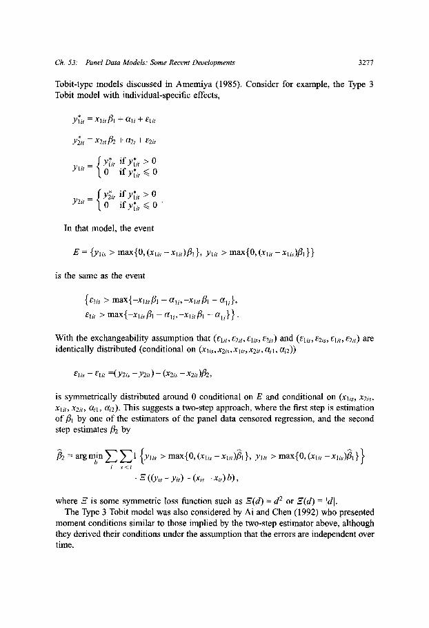
Ch 53: Panel Data Models: Some Recent Developments
Tobit-type models discussed in Amemiya ( 1985) Consider for example, the Type 3Tobit model with individual-specific effects,
lit = Xlit 31 + all + Elit
Y 2 it = X 2 it /2 + a 2 i + E 2 it
ylit = O if Yi > Oif Y 1 it O
Y 2 it = { O Yit if Yi < O O
In that model, the event
E = {ylis > max{ 0, (xis xlit)fi 1 1, lit > max{ 0,(xlit -Xlis)il}}
is the same as the event
{e lis > max{-x 1is 13 1 ali, -Xlitfl all),
Elit > max{-xli,s 31 ali,-xlitf 3 i ali)
With the exchangeability assumption that (lit, E 2 it, elis, e 2 is) and (li, E 2 is, Elit, e 2 it) areidentically distributed (conditional on (Xlis,X 2 is,Xlit,x 2 it, a Til, ai 2 ))
elis Elit =(Y 2 is Y 2 it) ( 2 is X 2 it)12,
is symmetrically distributed around O conditional on E and conditional on (xli S, X 2 is,xlit, x 2 it, ail, ai 2) This suggests a two-step approach, where the first step is estimationof 3 by one of the estimators of the panel data censored regression, and the secondstep estimates /32 by
2 = argmnin E l {Ylis >max{O,(xlis xlit)l}, ylit >max{ 0,(xlit-Xlis)~l}}i s<t
* (vis yit) (xi Xit) b),
where is some symmetric loss function such as H(d) = d 2 or E(d) = dl.The Type 3 Tobit model was also considered by Ai and Chen ( 1992) who presented
moment conditions similar to those implied by the two-step estimator above, althoughthey derived their conditions under the assumption that the errors are independent overtime.
3277
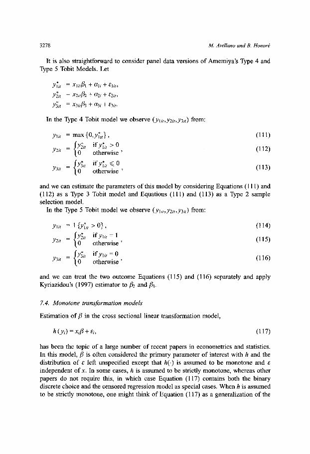
M Arellano and B Honor
It is also straightforward to consider panel data versions of Amemiya's Type 4 andType 5 Tobit Models Let
Yit = Xlitil + a Oli + Elit,
Y 2 it = X 2 it,2 + a 2 i + E 2 it,
Y 3 it = x/ ± a 3 i + 3 it 3
In the Type 4 Tobit model we observe (Ylit,Y 2 it,Y 3 it) from:
Ylit = max {O,yit,}, ( 111)
Y 2 it = 2 otherwise' ( 112)
otherwise' ( 113)
and we can estimate the parameters of this model by considering Equations ( 111) and( 112) as a Type 3 Tobit model and Equations ( 111) and ( 113) as a Type 2 sampleselection model.
In the Type 5 Tobit model we observe (Yli,Y 2 it,Y 3 it) from:
Ylit = 1 {Y~i, > O }, ( 114)
Y 3 it = { 43 it otherwise' ( 116)
and we can treat the two outcome Equations ( 115) and ( 116) separately and applyKyriazidou's ( 1997) estimator to 32 and /:33.
7.4 Monotone transformation models
Estimation of in the cross sectional linear transformation model,
h (yi) = xi/ + Ei, ( 117)
has been the topic of a large number of recent papers in econometrics and statistics.In this model, ,B is often considered the primary parameter of interest with h and thedistribution of E left unspecified except that h(-) is assumed to be monotone and independent of x In some cases, h is assumed to be strictly monotone, whereas otherpapers do not require this, in which case Equation ( 117) contains both the binarydiscrete choice and the censored regression model as special cases When h is assumedto be strictly monotone, one might think of Equation ( 117) as a generalization of the
3278
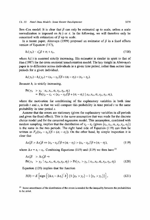
Ch 53: Panel Data Models: Some Recent Developments
Box-Cox model It is clear that If can only be estimated up to scale, unless a scalenormalization is imposed on h(-) or e In the following, we will therefore only beconcerned with estimation of /3 up to scale.
In a recent paper, Abrevaya ( 1999) proposed an estimator of /3 in a fixed effectsversion of Equation ( 117),
ht(yi,) = x'/3 + ai + Ei,, ( 118)
where h,( ) is assumed strictly increasing His estimator is similar in spirit to that ofHan ( 1987) for the cross sectional transformation model The key insight in Abrevaya'spaper is to difference across individuals in a given time period, rather than across timeperiods for a given individual,
h,(yi,) ht(yjt) = (xi xjt)l' + ( aj) + (it jj).
Because h, is strictly increasing,
Pr(yit > Yjt I xit,Xis, ai,)xjt,js, j)= Pr(Ejt eit < (xit xjt)/3 + (ai Ca) I Xit,Xis, ai,xjt, Xj, a ),
where the motivation for conditioning of the explanatory variables in both timeperiods t and s, is that we will compare this probability in time period t to the sameprobability in time period s.
Assume that the errors are stationary (given the explanatory variables in all periodsand given the fixed effect) This is the same assumption that was made for the discretechoice model and for the censored regression model This assumption, combined withrandom sampling, implies that the distribution of ej, it (given (xit,Xis, ai,xjt,xjs, aj))is the same in the two periods The right hand side of Equation ( 119) can then bewritten as Fij((xit Xjt)'l/ + (ai aj)) On the other hand, by simple inspection it isclear that
Ax/3 > Axj/3 X (xit -xjt)'/3 (i aj) > (xis Xjs)/p + (a j), ( 119)
where Ax = xt x Combining Equations ( 119) and ( 119) we then have 2 3
Ax': > Axj' X
Pr(yit > yjt x, xit, ai, xjs,xjt, aj) > Pr(ys > yjs xis, xit, ai, j, xjt, aj) ( 120)
Equation ( 120) implies that the function
S(b) E lsign ((Axi Axj)'b) ( 1 (yit > yjt) (yis > j))l ( 121)
23 Some smoothness of the distribution of the errors is needed for the inequality between the probabilitiesto be strict.
3279
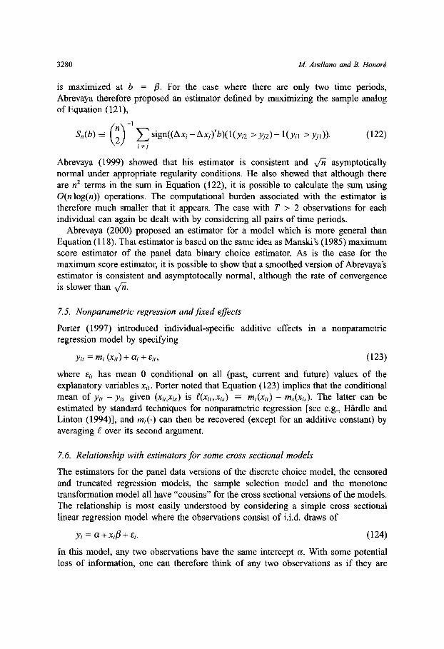
M Arellano and B Honor
is maximized at b = For the case where there are only two time periods,Abrevaya therefore proposed an estimator defined by maximizing the sample analogof Equation ( 121),
Sn(b) (n) Esign((Axi-Axj)b)(l(Yi 2 >Yj 2)-l(yil >Yjl)) ( 122)
Abrevaya ( 1999) showed that his estimator is consistent and /n asymptoticallynormal under appropriate regularity conditions He also showed that although thereare N 2 terms in the sum in Equation ( 122), it is possible to calculate the sum usingO(n log(n)) operations The computational burden associated with the estimator istherefore much smaller that it appears The case with T > 2 observations for eachindividual can again be dealt with by considering all pairs of time periods.
Abrevaya ( 2000) proposed an estimator for a model which is more general thanEquation ( 118) That estimator is based on the same idea as Manski's ( 1985) maximumscore estimator of the panel data binary choice estimator As is the case for themaximum score estimator, it is possible to show that a smoothed version of Abrevaya'sestimator is consistent and asymptotocally normal, although the rate of convergenceis slower than /.
7.5 Nonparametric regression andfixed effects
Porter ( 1997) introduced individual-specific additive effects in a nonparametricregression model by specifying
Yit = mt (xit) + ai + eit, ( 123)
where it, has mean 0 conditional on all (past, current and future) values of theexplanatory variables xi, Porter noted that Equation ( 123) implies that the conditionalmean of Yit Yis given (xit,xji) is (xji,xj) mt(xit,) ms(xis) The latter can beestimated by standard techniques for nonparametric regression lsee e g , Hirdle andLinton ( 1994)l, and m,( ) can then be recovered (except for an additive constant) byaveraging over its second argument.
7.6 Relationship with estimators for some cross sectional models
The estimators for the panel data versions of the discrete choice model, the censoredand truncated regression models, the sample selection model and the monotonetransformation model all have "cousins" for the cross sectional versions of the models.The relationship is most easily understood by considering a simple cross sectionallinear regression model where the observations consist of i i d draws of
Yi = a+xi + Ei ( 124)
In this model, any two observations have the same intercept a With some potentialloss of information, one can therefore think of any two observations as if they are
3280
Ch 53: Panel Data Models: Some Recent Developments
from a (static) linear panel data model with T = 2 This suggests forming all pairs ofobservations, and then estimating the slope-parameters /3 in Equation ( 124) by
= argmin ((y i -yj) (xi-x) b)2 .i <
It is an easy exersice to show that this is nothing but the OLS estimator of 3 in theregression of Equation ( 124).
The same logic can be applied to nonlinear models If the model under considerationis such that the parameter /3 can be estimated from a two-period panel by, say, someminimization problem
/3 =argmin Eg(yil,yi 2,xil,x 2 , b),
then a cross sectional version of the model can be estimated by
/3 = argmin Eg (yi,yj,xi,xj, b )i<j
Honor and Powell ( 1994) applied this insight to construct estimators for the crosssectional censored and truncated regression models based on the panel data estimatorsin Honor ( 1992).
The panel data estimators for the discrete choice and sample selection models alsohave cross sectional versions If Manski's ( 1987) estimator is applied to all pairs ofobservations from a cross sectional binary choice model, then the maximum rankcorrelation estimator of Han ( 1987) results (although his motivation was quite differentand his estimator applies to a more general class of transformations models) Likewise,applying the logic behind Kyriazidou's ( 1997) estimator of the sample selection modelto all pairs of observations in a cross sectional sample selection model results in theestimator proposed by Powell ( 1987) It is interesting to note that the cross sectionalestimator that uses all pairs of observations is x/ consistent in both of these cases,although the corresponding panel data estimator converges at a slower rate.
The situation is a little more complicated for the monotone transformation modelbecause the panel data estimator of that model is itself based on pairwise comparisonsacross individuals The cross sectional version that treats each pair of observations asif they came from a panel of length 2, is therefore based on comparing pairs of pairs,resulting in an estimator defined by a quadruple sum This estimator is analyzed inAbrevaya ( 1999).
Table 3 summarizes the relationship between the panel data estimators and theirpairwise comparison counterparts It also lists the estimator for the cross sectionalmodel which we find to be closest in spirit to the panel data estimator.
3281
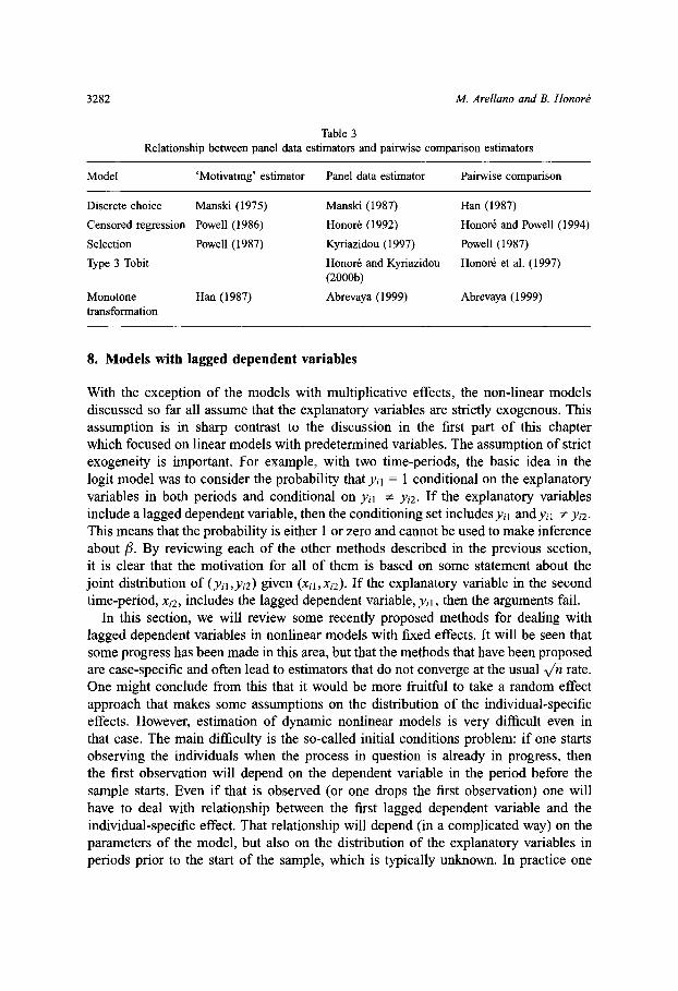
M Arellano and B Honors
Table 3Relationship between panel data estimators and pairwise comparison estimators
Model 'Motivating' estimator Panel data estimator Pairwise comparison
Discrete choice Manski ( 1975) Manski ( 1987) Han ( 1987)
Censored regression Powell ( 1986) Honor 6 ( 1992) Honor 6 and Powell ( 1994)
Selection Powell ( 1987) Kyriazidou ( 1997) Powell ( 1987)
Type 3 Tobit Honor 6 and Kyriazidou Honor 6 et al ( 1997)( 2000 b)
Monotone Han ( 1987) Abrevaya ( 1999) Abrevaya ( 1999)transformation
8 Models with lagged dependent variables
With the exception of the models with multiplicative effects, the non-linear modelsdiscussed so far all assume that the explanatory variables are strictly exogenous Thisassumption is in sharp contrast to the discussion in the first part of this chapterwhich focused on linear models with predetermined variables The assumption of strictexogeneity is important For example, with two time-periods, the basic idea in thelogit model was to consider the probability that Yil = 1 conditional on the explanatoryvariables in both periods and conditional on yil • yi 2 If the explanatory variablesinclude a lagged dependent variable, then the conditioning set includes Yil andyil I Yi 2.This means that the probability is either 1 or zero and cannot be used to make inferenceabout 3 By reviewing each of the other methods described in the previous section,it is clear that the motivation for all of them is based on some statement about thejoint distribution of (Yil,Yi 2) given (xil,Xi 2 ) If the explanatory variable in the secondtime-period, xi 2, includes the lagged dependent variable, yil, then the arguments fail.
In this section, we will review some recently proposed methods for dealing withlagged dependent variables in nonlinear models with fixed effects It will be seen thatsome progress has been made in this area, but that the methods that have been proposedare case-specific and often lead to estimators that do not converge at the usual /I rate.One might conclude from this that it would be more fruitful to take a random effectapproach that makes some assumptions on the distribution of the individual-specificeffects However, estimation of dynamic nonlinear models is very difficult even inthat case The main difficulty is the so-called initial conditions problem: if one startsobserving the individuals when the process in question is already in progress, thenthe first observation will depend on the dependent variable in the period before thesample starts Even if that is observed (or one drops the first observation) one willhave to deal with relationship between the first lagged dependent variable and theindividual-specific effect That relationship will depend (in a complicated way) on theparameters of the model, but also on the distribution of the explanatory variables inperiods prior to the start of the sample, which is typically unknown In practice one
3282
Ch 53: Panel Data Models: Some Recent Developments
might "solve" this problem by assuming a flexible functional form for the distributionof the first observation (see for example Heckman ( 1981 b) for a discussion of thisapproach) One case where one can ignore the initial conditions problem is when onecan reasonably assume that the process is observed from the start For example, if thedependent variable is labor supply and the sample consists of people observed (say)from the time they graduated from high school, then there will be no initial conditionsproblem.
In the next three sections we discuss some approaches that have been used togeneralize the limited dependent variable models discussed earlier to the case whereone of the explanatory variables is the lagged dependent variable Very little isknown about how to deal with general predetermined variables in the models that weconsider.
8.1 Discrete choice with state dependence
Including a lagged dependent variable among the explanatory variables in the discretechoice model with individual specific effects gives the model
Yit = 1 {xit: O Yi,t-l + ai + it O t = 1, , T; i = 1, ,n ( 125)
In its most general setting, this model allows for three sources of persistence(after controlling for the observed explanatory variable x) in the event described byyit, Persistence can be the result of serial correlation in the error term E, a resultof the "unobserved hererogeneity" a, or a result of true state dependence throughthe term yyi,t-l Distinguishing between these sources of persistence is important inmany situations because they have very different policy implications A policy thattemporarily increases the probabality that y = 1 will have different implications aboutfuture probabilities in a model with true state dependence than in model where thepersistence is due to unobserved heterogeneity See, for example, Heckman ( 1981 a) fora discussion of this Distinguishing between persistence due to state dependence anddue to heterogeneity is also important because they sometimes correspond to differenteconomic models For example, Chiappori and Salanie ( 2000) and Chiappori ( 1998)argue that it can be used to distinguish between moral hazard and adverse selection.The pricing system in the French automobile insurance market is such that theincentives for not having an accident are stronger if the driver has had fewer accidentsin the past This suggests that accident data should show true state dependence: havingan accident this period should lower the probability of an accident next period Onthe other hand adverse selection suggests that some drivers are permanantly morelikely to have accidents, which corresponds to the individual specific effect ai inEquation ( 125).
It is clear that even if the errors are serially independent, the conditions discussedearlier for conditional maximum likelihood estimation of the fixed effects logit modelare not satisfied because they implied that E in time period t is independent of the
3283
M Arellano and B Honors
explanatory variables in time period t 1, a condition which clearly fails when oneof the explanatory variables is the lagged dependent variable By the same argument,the conditions for the conditional maximum score estimator will not be satisfied inthe presence of a lagged dependent variable On the other hand it is also clear thatthe two sources of persistence in Equation ( 125) have very different implications Forexample consider the case where there are no other explanatory variables: if there isno "state dependence" (y = 0) then the sequence ( 0, 1,0, 1) would be as likely as thesequence (, 0, 0,1, 1) On the other hand, if y < O then the first sequence would be morelikely, whereas the second would be more likely if y > O As pointed out by Heckman( 1978), this suggests that one should be able to test for "no state dependence" in amodel like Equation ( 125) As will be seen below, this observation can also be usedto estimate y and /3 in Equation ( 125).
Consider first the special case of a logit model where the lagged dependent variableis the only explanatory variable,
Yit = 1 yyi, t I + a + it O} t = 1, ,T; i = 1, n,
where Eit is i i d , independent of ai, and logistically distributed Considering only thefirst three observations (and the initial condition), we have
Pr (yit = Ilai,yio , i,-) = +exp(yyi, +a) t = 1,2,3.1 + exp(yyi,t -I + a,)
It is then an easy exercise to see that
Pr(yi = 01 yil +yi 2 = 1, ai,Yio,Yi 3) =1 + exp (y(yi O -y))
which does not depend on a, and which can therefore be used to make inference ony lChamberlain ( 1978)l More generally, with T observations for each individual, theconditional distribution of (yil, , ir) given yil, T= 1 Iit and Yir is
P Yil, Yi T Yi ,Yit Yi T, aity , it l ,(d, (d,d,)E Bexp(Yz = 2 dtdtl)'
( 126)where B is the set of all sequences of zeros and ones that have ,T_ l di = IT=, Yit,di/ = Yil and dit = Yi Tr Magnac ( 1997) presents similar results for the multinomial logitversion of this model He also presents the conditional likelihood function for modelswith more than one lag.
Honor and Kyriazidou ( 2000 a) modify the calculations leading to the conditionalmaximum likelihood estimator of a fixed effects logit in such a way that it can beapplied to Equation ( 125) Specifically, assume that it in Equation ( 125) are i i d.
3284
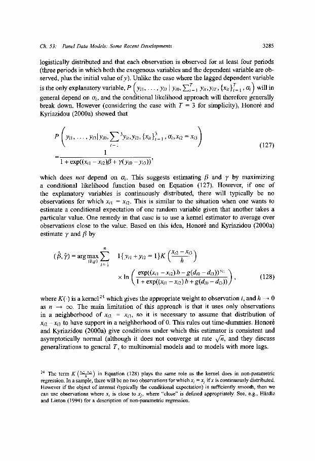
Ch 53: Panel Data Models: Some Recent Developments
logistically distributed and that each observation is observed for at least four periods(three periods in which both the exogenous variables and the dependent variable are ob-served, plus the initial value of y) Unlike the case where the lagged dependent variable
is the only explanatory variable, P (Yil, Yi , Yit,Yi T, t=, a) will ingeneral depend on ai, and the conditional likelihood approach will therefore generallybreak down However (considering the case with T = 3 for simplicity), Honor 6 andKyriazidou ( 2000 a) showed that
(Yil, , Yi 3 I Yio, 3yit,Yi 3, {xit} }=, a,,xi 2 = Xi 3)t= ( 127)
11 + exp((xil xi 2 )P + Y(Yio -Yi 3))'
which does not depend on ai This suggests estimating 3 and y by maximizinga conditional likelihood function based on Equation ( 127) However, if one ofthe explanatory variables is continuously distributed, there will typically be noobservations for which xil = xi 2 This is similar to the situation when one wants toestimate a conditional expectation of one random variable given that another takes aparticular value One remedy in that case is to use a kernel estimator to average overobservations close to the value Based on this idea, Honor 6 and Kyriazidou ( 2000 a)estimate y and / by
n
(/3, ')= argmax l{yil +Yi 2 = 1 } (Xi 2 Xi 3(bg) h
x N exp((xil Xi 2) b + g(dio d/ 3))Yi" ( 128)I + exp((xl Xi 2) b + g(dio di 3)) J
where K( ) is a kernel 24 which gives the appropriate weight to observation i, and h Oas N o The main limitation of this approach is that it uses only observationsin a neighborhood of Xi 2 = Xi 3, so it is necessary to assume that distribution ofxi 2 Xi 3 to have support in a neighborhood of O This rules out time-dummies Honorand Kyriazidou ( 2000 a) give conditions under which this estimator is consistent andasymptotically normal (although it does not converge at rate v/, and they discussgeneralizations to general T, to multinomial models and to models with more lags.
24 The term K ( 2 h 3 ) in Equation ( 128) plays the same role as the kernel does in non-parametricregression In a sample, there will be no two observations for which xi = xj if x is continuously distributed.However if the object of interest (typically the conditional expectation) is sufficiently smooth, then wecan use observations where xi is close to Xj, where "close" is defined appropriately See, e g , Hardleand Linton ( 1994) for a description of non-parametric regression.
3285
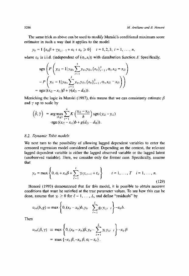
M Arellano and B Honored
The same trick as above can be used to modify Manski's conditional maximum scoreestimator in such a way that it applies to the model
Yit= xi + yyi, t + a + it O t = 1,2,3 ; i = 1, ,n,
where eit is i i d (independent of (ai,xi)) with distribution function F Specifically,
sgn P (Yi 2 = 1 Yi, Yit,Y 3 {Xt 1 } ,i,Xi 2 = Xi 3
-P (Yi = Yllyio, i Y,Yj 3,{x t},=l ,ai,xi 2 = Xi 3
= sgn ((Xi 2 Xil 13 + y(di 3 d)).
Mimicking the logic in Manski ( 1987), this means that we can consistenty estimate /3and y up to scale by
n
( ) =arg max K (Xi 2 h sgn(Yi 2 -Yil)
*sgn ((Xi 2 Xil)b + g(d 3 d)) ·
8.2 Dynamic Tobit models
We next turn to the possibility of allowing lagged dependent variables to enter thecensored regression model considered earlier Depending on the context, the relevantlagged dependent variable is either the lagged observed variable or the lagged latent(unobserved variable) Here, we consider only the former case Specifically, assumethat
Yit = max {O, ai +xit/3 -+ Ye Yi,t-e + EitF=l
( 129)Honor ( 1993) demonstrated that for this model, it is possible to obtain moment
conditions that must be satisfied at the true parameter values To see how this can bedone, assume that y > O for = 1, , L, and define "residuals" by
Ui,t(b,g)= max O,(xit -xi)b,yit Eg Yyi, t -xitb.
Then
.ist(/3 , y) max {O,(xixis)/,Yit -t Ye Yi, te} -xit 3
= max {-xit /3, -xi /3, ai + Eit }
3286
t = 1, , T i = 1, , n.
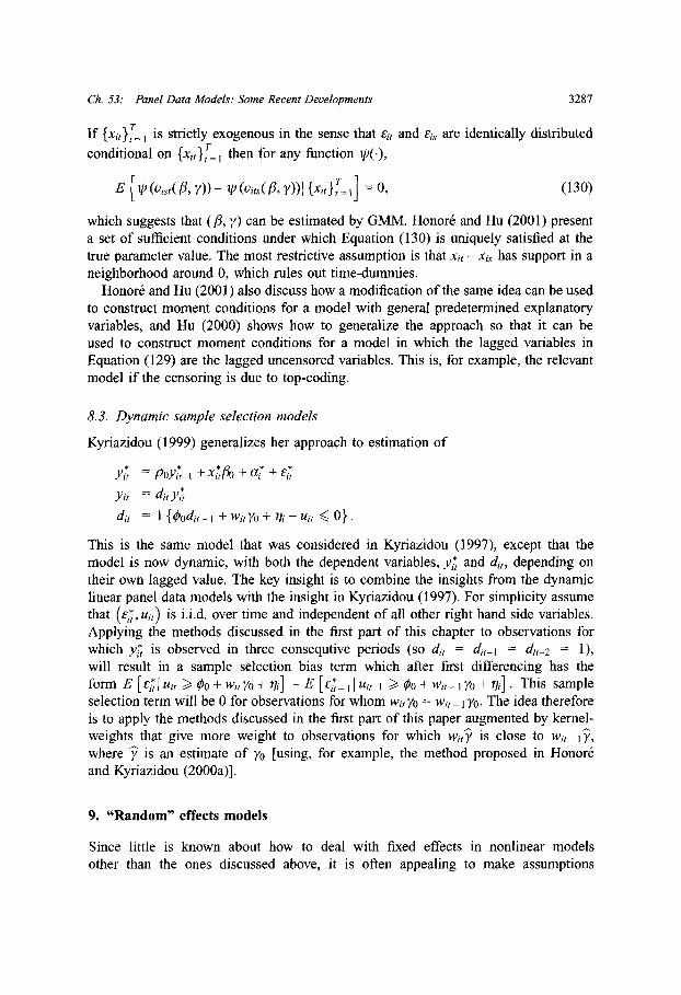
Ch 53: Panel Data Models: Some Recent Developments
If {xit,}= 1 is strictly exogenous in the sense that ei, and Eis are identically distributedconditional on {xi,}t=l then for any function ip(-),
E l ?(is,( 1,y)) (i(, ,y)){ {xir}T= 1l = 0, ( 130)
which suggests that (fi, y) can be estimated by GMM Honor and Hu ( 2001) presenta set of sufficient conditions under which Equation ( 130) is uniquely satisfied at thetrue parameter value The most restrictive assumption is that xit xi, has support in aneighborhood around 0, which rules out time-dummies.
Honor& and Hu ( 2001) also discuss how a modification of the same idea can be usedto construct moment conditions for a model with general predetermined explanatoryvariables, and Hu ( 2000) shows how to generalize the approach so that it can beused to construct moment conditions for a model in which the lagged variables inEquation ( 129) are the lagged uncensored variables This is, for example, the relevantmodel if the censoring is due to top-coding.
8.3 Dynamic sample selection models
Kyriazidou ( 1999) generalizes her approach to estimation of
Yit = Po Yt + xti + a + E,
yi, = dit y*t
di, = I {odit + wito + 7 li uit < O }.
This is the same model that was considered in Kyriazidou ( 1997), except that themodel is now dynamic, with both the dependent variables, Y*t and dit, depending ontheir own lagged value The key insight is to combine the insights from the dynamiclinear panel data models with the insight in Kyriazidou ( 1997) For simplicity assumethat (ei,, ui,) is i i d over time and independent of all other right hand side variables.Applying the methods discussed in the first part of this chapter to observations forwhich Y*t is observed in three consequtive periods (so di, = di = dit-2 = 1),will result in a sample selection bias term which after first differencing has theform E l Ei, Ulit q O O + Wit YO + lil E l _ ui 1l o + W ) Yo + il This sampleselection term will be 0 for observations for whom wit yo = wit Yo The idea thereforeis to apply the methods discussed in the first part of this paper augmented by kernel-weights that give more weight to observations for which wit, is close to wit -I,where is an estimate of yo lusing, for example, the method proposed in Honor&and Kyriazidou ( 2000 a)l.
9 "Random" effects models
Since little is known about how to deal with fixed effects in nonlinear modelsother than the ones discussed above, it is often appealing to make assumptions
3287
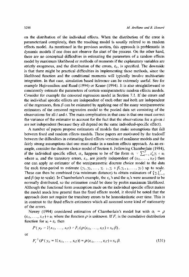
M Arellano and B Honors
on the distribution of the individual effects When the distribution of the error isparameterized completely, then the resulting model is usually refered to as randomeffects model As mentioned in the previous section, this approach is problematic indynamic models if one does not observe the start of the process On the other hand,there are no conceptual difficulties in estimating the parameters of a random effectsmodel by maximum likelihood or methods of moments if the explanatory variables arestrictly exogenous, and the distribution of the errors, eit, is specified The downsideis that there might be practical difficulties in implementing these methods, since thelikelihood function and the conditional moments will typically involve multivariateintegration In that case, simulation based inference can be extremely useful See forexample Hajivassiliou and Ruud ( 1994) or Keane ( 1994) It is also straightforward toconsistently estimate the parameters of certain semiparametric random effects models.Consider for example the censored regression model in Section 7 1 If the errors andthe individual specific effects are independent of each other and both are independentof the regressors, then fi can be estimated by applying one of the many semiparametricestimators of the censored regression model to the pooled data set consisting of theobservations for all i and t The main complication in that case is that one must correctthe variance of the estimator to account for the fact that the observations for a given iare not independent (because they all depend on the same individual-specific effect).
A number of papers propose estimators of models that make assumptions that fallbetween fixed and random effects models These papers are motivated by the tradeoffbetween the difficulties in estimating fixed effects versions of nonlinear models and thefairly strong assumptions that one must make in a random effects approach As an ex-ample, consider the discrete choice model of Section 6 Following Chamberlain ( 1984),if the individual specific effect, ai, happens to be of the form ai = r I= x¥, + ui
where ui and the transitory errors, ei,, are jointly independent of (xi, , xir) thenone can apply an estimator of the semiparametric discrete choice model to the datafor each time-period to estimate (l, 2 , Yt-i,Yt + y,, t+ , yr) up to scale.These can then be combined (via minimum distance) to obtain estimators of {y,7 t Iand 3 (up to scale) In Chamberlain's example, the eit's and the ui's were assumed to benormally distributed, so the estimation could be done by probit maximum likelihood.Although the functional form assumption made on the individual specific effect makesthe model much less general than the fixed effects model, it should be noted that theapproach does not require the transitory errors to be homoskedastic over time This isin contrast to the fixed effects estimators which all assumed some kind of stationarityof the errors.
Newey ( 1994) considered estimation of Chamberlain's model but with ai = p(xil, , xi T) + ui where the function p is unknown If F is the cumulative distributionfunction for ui + ei, then
P(Yit = I I xil, X ,X) = Ft(p(xl, x , XT) + ),
or
( 131)
3288
Ft (P(Y i, I 1 I il , · Xi T)) =Pp(Xi 1 , · · ,Xi T)++Xitfi-
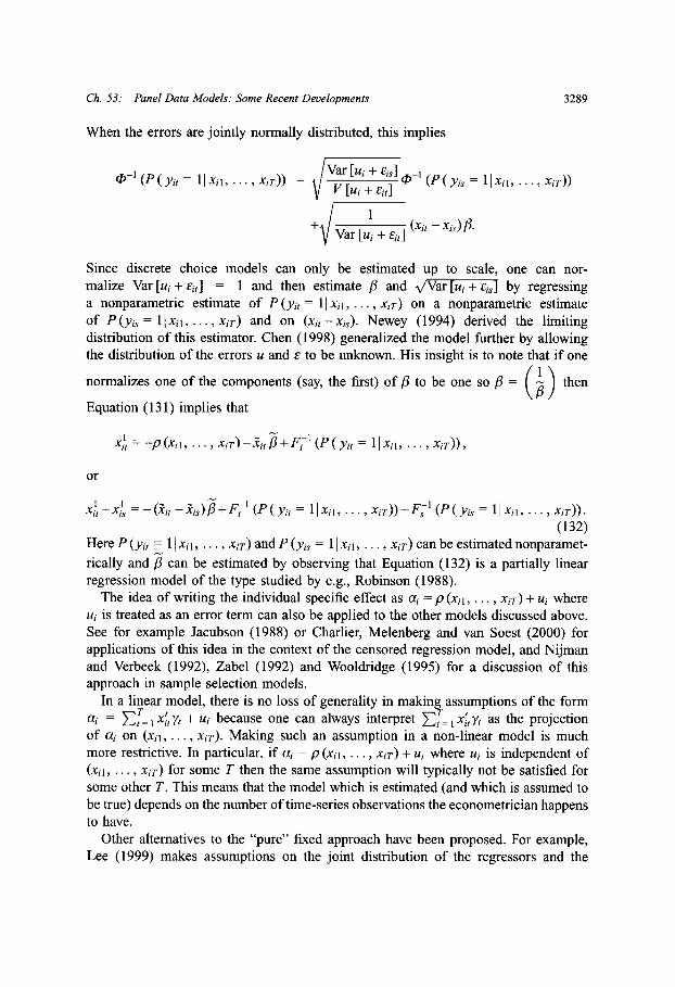
Ch 53: Panel Data Models: Some Recent Developments
When the errors are jointly normally distributed, this implies
Vas lui + il q (p ( Yis P= I I Xil *, X T))Xi T)) Vrlu, + it
+ Var lui t (xi)
Since discrete choice models can only be estimated up to scale, one can nor-malize Var lui + il = 1 and then estimate /3 and /Var lu +eisl by regressinga nonparametric estimate of P(yit = Ix I, , xi T) on a nonparametric estimateof P(Yis = 1 xil, , ir T) and on (xi, -xi,) Newey ( 1994) derived the limitingdistribution of this estimator Chen ( 1998) generalized the model further by allowingthe distribution of the errors u and E to be unknown His insight is to note that if one
normalizes one of the components (say, the first) of 3 to be one so = ( then
Equation ( 131) implies that
or
I I (P (Yis = I Xil, Xi T)) ,it -xs = it is)+Ft -'(P(y 1 =II xl, , Xi T))-F l (P(yis = llxl, , Xir)).
( 132)Here P (yi, = 1 xil, , Xi T) and P (yi, = l Xi, , r) can be estimated nonparamet-rically and /3 can be estimated by observing that Equation ( 132) is a partially linearregression model of the type studied by e g , Robinson ( 1988).
The idea of writing the individual specific effect as a = p (Xil, , Xi T) + Ui whereui is treated as an error term can also be applied to the other models discussed above.See for example Jacubson ( 1988) or Charlier, Melenberg and van Soest ( 2000) forapplications of this idea in the context of the censored regression model, and Nijmanand Verbeek ( 1992), Zabel ( 1992) and Wooldridge ( 1995) for a discussion of thisapproach in sample selection models.
In a linear model, there is no loss of generality in making assumptions of the form= ET xta, = x 1 ,t Yr + ui because one can always interpret 5 T= I, ty as the projection
of ai on (Xil, , T) Making such an assumption in a non-linear model is muchmore restrictive In particular, if ai = p(xl, , Xir) + ui where ui is independent of(xil, , Xi) for some T then the same assumption will typically not be satisfied forsome other T This means that the model which is estimated (and which is assumed tobe true) depends on the number of time-series observations the econometrician happensto have.
Other alternatives to the "pure" fixed approach have been proposed For example,Lee ( 1999) makes assumptions on the joint distribution of the regressors and the
3289
M Arellano and B Honors
individual specific effects which allow him to construct a maximum rank correlation-type estimator of the static discrete choice panel data model Honor and Lewbel( 2000) exploit the assumption that one of the regressors is independent of the individualspecific effect to construct an estimator of a discrete choice panel data model withpredetermined explanatory variables.
10 Concluding remarks
Our discussion has focused on two of the developments in panel data econometricssince the Handbook chapter by Chamberlain ( 1984) In the first part of the paperwe have reviewed linear panel data models with predetermined variables, and in thesecond we have discussed methods for dealing with nonlinear panel data models.Unfortunately, the intersection of these two literatures is very small With the exceptionof multiplicative models and models where the only source of "predeterminedness"is lagged dependent variables, almost nothing is known about nonlinear models withgeneral predetermined variables One step in this direction was taken by Arellano andCarrasco ( 1996) This is an exciting area for future research.
References
Abowd, J M , and D Card ( 1989), "On the covariance structure of earnings and hours changes",Econometrica 57:411-445.
Abrevaya, J ( 1999), "Leapfrog estimation of a fixed-effects model with unknown transformation of thedependent variable", Journal of Econometrics 93 ( 2):203-228.
Abrevaya, J ( 2000), "Rank estimation of a generalized fixed-effects regression model", Journal ofEconometrics 95 ( 1):1-23.
Ahn, S , and P Schmidt ( 1995), "Efficient estimation of models for dynamic panel data", Journal ofEconometrics 68:5-27.
Ai, C , and C Chen ( 1992), "Estimation of a fixed effect bivariate censored regression model", EconomicLetters 40:403-406.
Allenby, G M , and P E Rossi ( 1999), "Marketing models of consumer heterogeneity", Journal ofEconometrics 89:57-78.
Alonso-Borrego, C , and M Arellano ( 1999), "Symmetrically normalized instrumental-variable estimationusing panel data", Journal of Business & Economic Statistics 17:36-49.
Alvarez, J , and M Arellano ( 1998), "The time series and cross-section asymptotics of dynamic paneldata estimators", Working Paper 9808 (CEMFI, Madrid).
Amemiya, T ( 1985), Advanced Econometrics (Harvard University Press).Amemiya, T , and T E Ma Curdy ( 1986), "Instrumental-variable estimation of an error-components
model", Econometrica 54:869-881.Andersen, E B ( 1970), "Asymptotic properties of conditional maximum likelihood estimators", Journal
of the Royal Statistical Society, Series B 32:283-301.Anderson, T W , and C Hsiao ( 1981), "Estimation of dynamic models with error components", Journal
of the American Statistical Association 76:598-606.Anderson, TW , and C Hsiao ( 1982), "Formulation and estimation of dynamic models using panel data",
Journal of Econometrics 18:47-82.
3290
Ch 53: Panel Data Models: Some Recent Developments
Anderson, T W, N Kunitomo and T Sawa ( 1982), "Evaluation of the distribution function of the limitedinformation maximum likelihood estimator", Econometrica 50 ( 4):1009-1027.
Arellano, M ( 1990), "Testing for autocorrelation in dynamic random effects models", Review ofEconomic Studies 57:127-134.
Arellano, M ( 1993), "On the testing of correlated effects with panel data", Journal of Econometrics59:87-97.
Arellano, M , and S R Bond ( 1988), "Dynamic panel data estimation using DPD A guide for users",Working Paper 88/15, (Institute for Fiscal Studies, London).
Arellano, M , and S R Bond ( 1991), "Some tests of specification for panel data: Monte Carlo evidenceand an application to employment equations", Review of Economic Studies 58:277-297.
Arellano, M , and O Bover ( 1995), "Another look at the instrumental-variable estimation of error-components models", Journal of Econometrics 68:29-51.
Arellano, M , and R Carrasco ( 1996), "Binary choice panel data models with predetermined variables",Working Paper 9618 (CEMFI, Madrid).
Ashenfelter, O , and D Card ( 1985), "Using the longitudinal structure of earnings to estimate the effectof training programs", Review of Economics and Statistics 67:648-660.
Back, K , and D P Brown ( 1993), "Implied probabilities in GMM estimators", Econometrica 61:971-975.Baltagi, B ( 1995), Econometric Analysis of Panel Data (John Wiley and Sons Ltd )Baltagi, B , J Hidalgo and Q Li ( 1996), "A nonparametric poolability test", Journal of Econometrics
75:345-367.Becker, G , M Grossman and K Murphy ( 1994), "An empirical analysis of cigarette addiction", American
Economic Review 84:396-418.Bekker, P A ( 1994), "Alternative approximations to the distributions of instrumental variable estimators",
Econometrica 62:657-681.Bhargava, A , and J D Sargan ( 1983), "Estimating dynamic random effects models from panel data
covering short time periods", Econometrica 51:1635-1659.Blundell, R , and S Bond ( 1998), "Initial conditions and moment restrictions in dynamic panel data
models", Journal of Econometrics 87:115-143.Blundell, R , and S Bond ( 1999), "GMM estimation with persistent panel data: an application to
production functions", Working Paper W 99/4 (Institute for Fiscal Studies, London).Blundell, R , S Bond, M P Devereux and E Schiantarelli ( 1992), "Investment and Tobin's Q: evidence
from company panel data", Journal of Econometrics 51:233-257.Blundell, R , R Griffith and E Windmeijer ( 1997), "Individual effects and dynamic count data",
Unpublished manuscript (University College London).Bond, S , and C Meghir ( 1994), "Dynamic investment models and the firm's financial policy", Review
of Economic Studies 61:197-222.Bover, O ( 1991), "Relaxing intertemporal separability: a rational habits model of labor supply estimated
from panel data", Journal of Labor Economics 9:85-100.Breusch, T S , G E Mizon and P Schmidt ( 1989), "Efficient estimation using panel data", Econometrica
57:695-700.Browning, M ( 1992), "Children and household economic behaviour", Journal of Economic Literature
30:1434-1475.Canova, E, and A Marcet ( 1995), "The poor stay poor: nonconvergence across countries and regions",
Economics Working Paper 137 (Universitat Pompeu Fabra, Barcelona).Carrasco, R ( 1998), "Binary choice with binary endogenous regressors in panel data: estimating the
effect of fertility on female labour participation", Working Paper 9805 (CEMFI, Madrid).Cavanagh, C L ( 1987), "The limiting behavior of estimators defined by optimization", Unpublished
manuscript (Department of Economics, Harvard University).Chamberlain, G ( 1978), "On the use of panel data", Unpublished manuscript (Department of Economics,
Harvard University).
3291
M Arellano and B Honors
Chamberlain, G ( 1980), "Analysis of covariance with qualitative data", Review of Economic Studies47:225-238.
Chamberlain, G ( 1982 a), "Multivariate regression models for panel data", Journal of Econometrics18:5-46.
Chamberlain, G ( 1982 b), "The general equivalence of Granger and Sims causality", Econometrica50:569-581.
Chamberlain, G ( 1984), "Panel data", in: Z Griliches and M D Intriligator, eds , Handbook ofEconometrics, Vol 2 (Elsevier Science, Amsterdam).
Chamberlain, G ( 1987), "Asymptotic efficiency in estimation with conditional moment restrictions",Journal of Econometrics 34:305-334.
Chamberlain, G ( 1992 a), "Efficiency bounds for semiparametric regression", Econometrica 60:567-596.Chamberlain, G ( 1992 b), "Comment: sequential moment restrictions in panel data", Journal of Business
& Economic Statistics 10:20-26.Chamberlain, G ( 1993), "Feedback in panel data models", Unpublished manuscript (Department of
Economics, Harvard University).Chamberlain, G , and K Hirano ( 1999), "Predictive distributions based on longitudinal earnings data",
Annales d'Economie et de Statistique 55-56:211-242.Charlier, E , B Melenberg and A van Soest ( 1995), "A smoothed maximum score estimator for the
binary choice panel data model and an application to labour force participation", Statistica Neerlandica49:324-342.
Charlier, E , B Melenberg and A van Soest ( 2000), "Estimation of a censored regression panel datamodel using conditional moments restrictions efficiently", Journal of Econometrics 95 ( 1):25-56.
Chen, S ( 1998), "Root-N consistent estimation of a panel data sample selection model", unpublishedmanuscript (The Hong Kong University of Science and Technology).
Chen, S , J J Heckman and E Vytlacil ( 1998), "Identification and /;i estimation of semiparametricpanel data models with binary variables and latent factors", Unpublished manuscript (Department ofEconomics, University of Chicago).
Chiappori, P -A ( 1998), "Econometric models of insurance under asymmetric information", Unpublishedmanuscript (Department of Economics, University of Chicago).
Chiappori, P -A , and B Salanie ( 2000), "Testing for adverse selection in insurance markets", Journal ofPolitical Economy 108:56-78.
Collado, M D ( 1997), "Estimating dynamic models from time series of independent cross-sections",Journal of Econometrics 82:37-62.
Crepon, B , E Kramarz and A Trognon ( 1997), "Parameters of interest, nuisance parameters andorthogonality conditions An application to autoregressive error component models", Journal ofEconometrics 82:135-156.
Deaton, A ( 1985), "Panel data from time series of cross-sections", Journal of Econometrics 30:109-126.Geweke, J , and M Keane ( 2000), "An empirical analysis of earnings dynamics among men in the PSID:
1968-1989 ", Journal of Econometrics 96:293-356.Granger, C W J ( 1969), "Investigating causal relations by econometric models and cross-spectral methods",
Econometrica 37:424-438.Griliches, Z , and J A Hausman ( 1986), "Errors in variables in panel data", Journal of Econometrics
31:93-118.Hahn, J ( 1997), "Efficient estimation of panel data models with sequential moment restrictions", Journal
of Econometrics 79:1-21.Hahn, J ( 1998), "Asymptotically unbiased inference of dynamic panel data model with fixed effects
when both N and T are large", Unpublished manuscript (University of Pennsylvania).Hajivassiliou, V, and D McFadden ( 1990), "The method of simulated scores for the estimation of LDV
models with an application to external debt crisis", Cowles Foundation Discussion Paper 967 (CowlesFoundation for Research in Economics, Yale University).
3292

Ch 53: Panel Data Models: Some Recent Developments
Hajivassiliou, V, and P A Ruud ( 1994), "Classical estimation methods for LDV models using simulation",in: R E Engle and D L McFadden, eds , Handbook of Econometrics, Vol 4 (Elsevier, Amsterdam)Ch 40.
Hall, R E , and ES Mishkin ( 1982), "The sensitivity of consumption to transitory income: estimatesfrom panel data on households", Econometrica 50:461-481.
Han, A K ( 1987), "Non-parametric analysis of a generalized regression model: the maximum rankcorrelation estimator", Journal of Econometrics 35:303-316.
Hansen, L P ( 1982), "Large sample properties of generalized method of moments estimators",Econometrica 50:1029-1054.
Hansen, L P , J Heaton and A Yaron ( 1996), "Finite sample properties of some alternative GMMestimators", Journal of Business & Economic Statistics 14:262-280.
Hurdle, W , and O Linton ( 1994), "Applied nonparametric methods", in: R E Engle and D L McFadden,eds , Handbook of Econometrics, Vol 4 (Elsevier, Amsterdam) Ch 38.
Hausman, J A , and W E Taylor ( 1981), "Panel data and unobservable individual effects", Econometrica49:1377-1398.
Hausman, J A , B Hall and Z Griliches ( 1984), "Econometric models for count data with an applicationto the patents-R&D relationship", Econometrica 52 ( 4):909-938.
Hayashi, E, and T Inoue ( 1991), "The relation between firm growth and Q with multiple capital goods:theory and evidence from panel data on Japanese firms", Econometrica 59:731-753.
Hayashi, E, and C A Sims ( 1983), "Nearly efficient estimation of time series models with predetermined,but not exogenous, instruments", Econometrica 51:783-798.
Heckman, J J ( 1976), "The common structure of statistical models of truncation, sample selection andlimited dependent variables and a simple estimator for such models", Annals of Economic and SocialMeasurement 15:475-492.
Heckman, J J ( 1978), "Simple statistical models for discrete panel data developed and applied to tests ofthe hypothesis of true state dependence against the hypothesis of spurious state dependence", Annalesde I'INSEE 30-31:227-269
Heckman, J J ( 1979), "Sample selection bias as a specification error", Econometrica 47:153-161.Heckman, J J ( 1981 a), "Statistical models for discrete panel data", in: C F Manski and D McFadden,
eds , Structural Analysis of Discrete Panel Data with Econometric Applications (MIT Press).Heckman, J J ( 1981 b), "The incedental parameters problem and the problem of initial conditions in
estimating a discrete time-discrete data stochastic process", in: C E Manski and D McFadden eds ,Structural Analysis of Discrete Panel Data with Econometric Applications (MIT Press).
Heckman, J J , and T E Ma Curdy ( 1980), "A life cycle model of female labour supply", Review ofEconomic Studies 47:47-74.
Hillier, G H ( 1990), "On the normalization of structural equations: properties of direction estimators",Econometrica 58:1181-1194.
Holtz-Eakin, D , W K Newey and H Rosen ( 1988), "Estimating vector autoregressions with panel data",Econometrica 56:1371-1395.
Honor, B E ( 1992), "Trimmed lad and least squares estimation of truncated and censored regressionmodels with fixed effects", Econometrica 60:533-565.
Honored, B E ( 1993), "Orthogonality conditions for tobit models with fixed effects and lagged dependentvariables", Journal of Econometrics 59:35-61.
Honored, B E , and L Hu ( 2001), "Estimation of censored regression models with endogeneity",Unpublished manuscript (Department of Economics, Princeton University).
Honor, B E , and E Kyriazidou ( 2000 a), "Panel data discrete choice models with lagged dependentvariables", Econometrica 68 ( 4):839-874.
Honored, B E , and E Kyriazidou ( 2000 b), "Estimation of Tobit-type models with individual specificeffects", Econometric Reviews 19 ( 3):341-366.
Honor, B E , and A Lewbel ( 2000), "Semiparametric binary choice panel data models without strictlyexogeneous regressors", Unpublished manuscript (Department of Economics, Princeton University).
3293
M Arellano and B Honors
Honor, B E , and J L Powell ( 1994), "Pairwise difference estimators of censored and truncated regressionmodels", Journal of Econometrics 64 ( 2):241-278.
Honor, B E , E Kyriazidou and C Udry ( 1997), "Estimation of type 3 Tobit models using symmetrictrimming and pairwise comparisons", Journal of Econometrics 76:107-128.
Horowitz, J L ( 1992), "A smoothed maximum score estimator for the binary response model",Econometrica 60:505-531.
Horowitz, J L , and M Markatou ( 1996), "Semiparametric estimation of regression models for paneldata", Review of Economic Studies 63:145-168.
Hsiao, C ( 1986), Econometric Analysis of Panel Data (Cambridge University Press).Hu, L ( 2000), "Estimating a censored dynamic panel data model with an application to earnings
dynamics", Unpublished manuscript (Department of Economics, Northwestern University).Imbens, G ( 1997), "One-step estimators for over-identified generalized method of moments models",
Review of Economic Studies 64:359-383.Imbens, G , R Spady and P Johnson ( 1998), "Information theoretic approaches to inference in moment
condition models", Econometrica 66:333-357.Jacubson, G ( 1988), "The sensitivity of labor supply parameter estimates to unobserved individual
effects: fixed and random effects estimates in a nonlinear model using panel data", Journal of LaborEconomics 6:302-329.
Kao, C ( 1999), "Spurious regression and residual-based tests for cointegration in panel data", Journalof Econometrics 90:1-44.
Keane, M ( 1993), "Simulation estimation for panel data models with limited dependent variables", in:G.S Maddala, C R Rao and H D Vinod, eds , Handbook of Statistics, Vol 11 (Elsevier Science,Amsterdam).
Keane, M ( 1994), "A computationally practical simulation estimator for panel data", Econometrica62:95-116.
Keane, M , and D E Runkle ( 1992), "On the estimation of panel-data models with serial correlationwhen instruments are not strictly exogenous", Journal of Business & Economic Statistics 10:1-9.
Kim, J , and D Pollard ( 1990), "Cube root asymptotics", Annals of Statistics 18:191-219.Kiviet, J E ( 1995), "On bias, inconsistency, and efficiency of various estimators in dynamic panel data
models", Journal of Econometrics 68:53-78.Kunitomo, N ( 1980), "Asymptotic expansions of the distribution of estimators in a linear functional
relationship and simultaneous equations", Journal of the American Statistical Society 75:693-700.Kyriazidou, E ( 1995), "Essays in estimation and testing of econometric models", Ph D dissertation
(Northwestern University).Kyriazidou, E ( 1997), "Estimation of a panel data sample selection model", Econometrica 65:1335-1364.Kyriazidou, E ( 1999), "Estimation of dynamic panel data sample selection models", Unpublished
manuscript (Department of Economics, University of Chicago).Lancaster, T ( 1997), "Orthogonal parameters in panel data", Working Paper No 97-12 (Brown University,
Department of Economics).Lee, M -J ( 1999), "A root-n consistent semiparametric estimator for related effect binary response panel
data", Econometrica 67:427-434.Li, Q , and C Hsiao ( 1998), "Testing serial correlation in semiparametric panel data models", Journal
of Econometrics 87:207-237.Li, Q , and T Stengos ( 1996), "Semiparametric estimation of partially linear panel data models", Journal
of Econometrics 71:389-397.Lillard, L A , and R J Willis ( 1978), "Dynamic aspects of earnings mobility", Econometrica 46:
985-1012.Ma Curdy, T E ( 1982), "The use of time series processes to model the error structure of earnings in a
longitudinal data analysis", Journal of Econometrics 18:83-114.Magnac, T ( 1997), "State dependence and heterogeneity in youth employment histories", Working Paper
(INRA and CREST, Paris).
3294
Ch 53: Panel Data Models: Some Recent Developments
Manski, C E ( 1975), "The maximum score estimation of the stochastic utility model of choice", Journalof Econometrics 3:205-228.
Manski, C E ( 1985), "Semiparametric analysis of discrete response: asymptotic properties of the maximumscore estimator", Journal of Econometrics 27:313-333.
Manski, C F ( 1987), "Semiparametric analysis of random effects linear models from binary panel data",Econometrica 55:357-362.
Moffitt, R ( 1993), "Identification and estimation of dynamic models with a time series of repeatedcross-sections", Journal of Econometrics 59:99-123.
Morimune, K ( 1983), "Approximate distributions of k-class estimators when the degree ofoveridentifiability is large compared with the sample size", Econometrica 51:821-841.
Newey, WK ( 1994), "The asymptotic variance of semiparametric estimators", Econometrica62:1349-1382.
Neyman, J , and E L Scott ( 1948), "Consistent estimates based on partially consistent observations",Econometrica 16:1-32.
Nickell, S J ( 1981), "Biases in dynamic models with fixed effects", Econometrica 49:1417-1426.Nijman, T , and M Verbeek ( 1992), "Nonresponse in panel data: the impact on estimates of a life cycle
consumption function", Journal of Applied Econometrics 7:243-257.Pesaran, M H , and R Smith ( 1995), "Estimating long-run relationships from dynamic heterogeneous
panels", Journal of Econometrics 68:79-113.Phillips, P C B ( 1983), "Exact small sample theory in the simultaneous equations model", in: Z Griliches
and M D Intriligator, eds , Handbook of Econometrics, Vol 1 (North-Holland, Amsterdam) Ch 8.Phillips, P C B , and H R Moon ( 1999), "Linear regression limit theory for nonstationary panel data",
Econometrica 67:1057-1111.Porter, J ( 1997), "Nonparametric regression estimation for a panel data model with additive individual
effects", Unpublished (Harvard University).Powell, J L ( 1986), "Symmetrically trimmed least squares estimation for Tobit models", Econometrica
54:1435-1460.Powell, J L ( 1987), "Semiparametric estimation of bivariate latent models", Working Paper no 8704
(Social Systems Research Institute, University of Wisconsin-Madison).Powell, J L ( 1994), "Estimation of semiparametric models", in: R E Engle and D L McFadden, eds ,
Handbook of Econometrics, Vol 4 (Elsevier, Amsterdam) Ch 41.Qin, J , and J Lawless ( 1994), "Empirical likelihood and general estimating equations", Annals of
Statistics 22:300-325.Rasch, G ( 1960), Probabilistic Models for Some Intelligence and Attainment Tests (Denmarks
Padagogiske Institut, Copenhagen).Rasch, G ( 1961), "On the general laws and the meaning of measurement in psychology", Proceedings
of the Fourth Berkeley Symposium on Mathematical Statistics and Probability, Vol 4 (University ofCalifornia Press, Berkeley and Los Angeles).
Robinson, PM ( 1988), "Root-n-consistent semiparametric regression", Econometrica 56:931-954.Runkle, D E ( 1991), "Liquidity constraints and the permanent income hypothesis: evidence from panel
data", Journal of Monetary Economics 97:73-98.Sargan, J D ( 1958), "The estimation of economic relationships using instrumental variables",
Econometrica 26:393-415.Schmidt, P, S C Ahn and D Wyhowski ( 1992), "Comment", Journal of Business & Economic Statistics
10:10-14.Sims, C A ( 1972), "Money, income, and causality", American Economic Review 62:540-552.Wooldridge, J M ( 1995), "Selection corrections for panel data models under conditional mean
independence assumptions", Journal of Econometrics 68:115-132.Wooldridge, J M ( 1997), "Multiplicative panel data models without the strict exogeneity assumption",
Econometric Theory 13:667-678.
3295

3296 M Arellano and B Honors
Zabel, J E ( 1992), "Estimating fixed and random effects models with selectivity", Economic Letters40:269-272.
Zeldes, S P ( 1989), "Consumption and liquidity constraints: an empirical investigation", Journal ofPolitical Economy 97:305-346.
Ziliak, J P ( 1997), "Efficient estimation with panel data when instruments are predetermined: anempirical comparison of moment-condition estimators", Journal of Business & Economic Statistics15:419-431.