PALEOCEANOGRAPHY, VOL. 1, NO. 1, PAGES 43-66, MARCH 1986

LATE QUATERNARY PALEOCEANOGRAPHY OF THE TROPICAL ATLANTIC, 1: SPATIAL VARIABILITY OF ANNUAL MEAN SEA-SURFACE

TEMPERATURES, 0-20,000 YEARS B.P.

Alan C. Mix

College of Oceanography, Oregon State University, Corvallis, OR 97331

William F. Ruddiman

Lamont-Doherty Geological Observatory, Columbia University, Palisades, NY 10964

Andrew Mcintyre

Department of Earth and Environmental Sciences, Queens College, City University, New York, NY

Abstract. At least two modes of glacial-interglacial climate change have existed within the tropical Atlantic Ocean during the last 20,000 years. The first mode (defined by cold glacial and warm interglacial conditions) occurred symmetrically north and south of the equator and dominated the eastern boundary currents and tropical upwelling areas. This pattern suggests that mode 1 is driven by a glacial modification of surface winds in both hemispheres. The second mode of oceanic climate change, defined by temperature extremes centered on the deglaciation, was hemispherically asymmetrical, with the northern tropical Atlantic relatively cold and the southern tropical Atlantic relatively warm during deglaciation. A likely cause for this pattern of variation is a reduction of the presently northward cross-equatorial heat flux during deglaciation. No single mechanism accounts for all the data. Potential contributors to oceanic climate changes are linkage to high-latitude climates, modification of mon- soonal winds by ice sheet and/or insolation changes, atmospheric CO2 and greenhouse effects, indirect effects of glacial meltwater, and variations in thermohaline overturn of the oceans.

•Previously at Lamont-Doherty Geological Observatory, and Department of Geology, Columbia University, Palisades, New York.

2Also at Lamont-Doherty Geological Observatory, Palisades, New York.

Copyright 1986 by the American Geophysical Union.

Paper number 5P0836. 0883-8305 / 86/005 P-0836510.00

INTRODUCTION

The tropical oceans act as a solar collector and heat source for the earth's climate. Heat collected here is

advected away from the tropics in oceanic currents. Some of this heat is transferred to the atmosphere in the middle latitudes [Von der Haar and Oort, 1973] and is thus transported to the polar regions, where net radiative heat loss occurs.

This paper examines thermal variability of the tropical Atlantic Ocean during the transition from the last glaciation to the modern interglaciation between 20,000 years B.P. and the present. Our approach is to study spatial variability of tropical Atlantic paleotemperatures estimated from fossil foraminiferal assemblages. By determining the spatial effects of climate changes, we attempt to trace patterns of variability to the mechanisms governing their occurrence. Topics to be addressed include (1) linkage between northern and southern hemisphere oceanic climate, (2) variations in Atlantic interhemispheric heat transport, and (3) relationships between low-latitude and high-latitude climate changes on a glacial-interglacial time scale.

PHYSICAL OCEANOGRAPHY

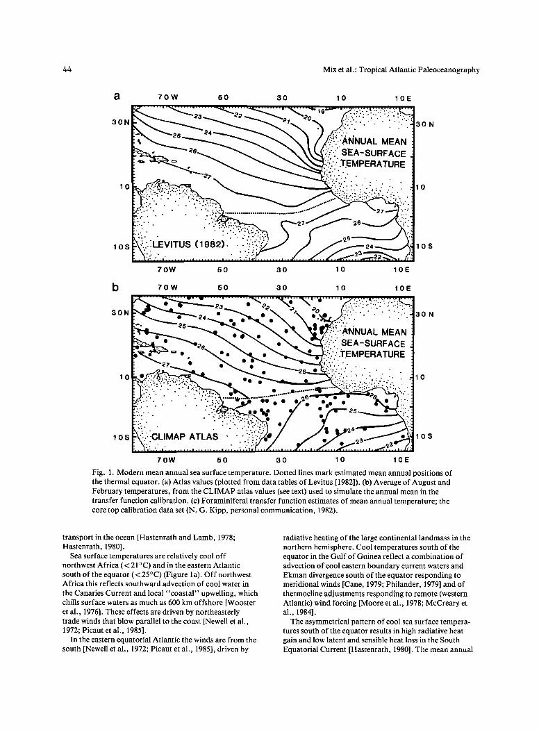
The modern sea surface temperatures of the tropical Atlantic Ocean are controlled by the winds. On an annual average, warmest temperatures (> 27øC) occur mostly in the western equatorial Atlantic (Figure la), especially in the northern hemisphere [Levitus, 1982; Reynolds, 1982]. This reflects radiative heating of surface waters advected westward in the North and South Equatorial currents, the northern hemisphere position of the Intertropical Conver- gence Zone (!TCZ), and northward cross-equatorial heat

4/4 Mix et al.' Tropical Atlantic Paleoceanography

a 70W 50 30 10 10E

70W 50 30 10 10E

--' 30 N

10

10S

b 70W 50 30 10 10E

30N

10

10S

ß

25

":CLIMAP ATLAS .. ß

ß

ß

ßß

ß

ß ß ß ß

ß

., ß . ß

ß .

ß .

ß .

ii'"'.•NNUA L MEAN ß ::;..':'." SEA-SURFACE "'.TEMPERATURE

ß . ß

.

,•. •ø .' o . ß ß . .

30N

10

10S

70W 50 30 10 10E

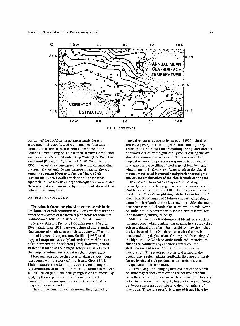
Fig. 1. Modern mean annual sea surface temperature. Dotted lines mark estimated mean annual positions of the thermal equator. (a) Atlas values (plotted from data tables of Levitus [1982]). (b) Average of August and February temperatures, from the CLIMAP atlas values (see text) used to simulate the annual mean in the transfer function calibration. (c) Foraminiferal transfer function estimates of mean annual temperature; the core top calibration data set (N. G. Kipp, personal communication, 1982).

transport in the ocean [Hastenrath and Lamb, 1978; Hastenrath, 1980].

Sea surface temperatures are relatively cool off northwest Africa ( < 21 ø C) and in the eastern Atlantic south of the equator (<25øC) (Figure la). Off northwest Africa this reflects southward advection of cool water in

the Canaries Current and local "coastal" upwelling, which chills surface waters as much as 600 km offshore [Wooster et al., 1976]. These effects are driven by northeasterly trade winds that blow parallel to the coast [Newell et al., 1972; Picaut et al., 1985].

In the eastern equatorial Atlantic the winds are from the south [Newell et al., 1972; Picaut et al., 1985], driven by

radiative heating of the large continental landmass in the northern hemisphere. Cool temperatures south of the equator in the Gulf of Guinea reflect a combination of advection of cool eastern boundary current waters and Ekman divergence south of the equator responding to meridional winds [Cane, 1979; Philander, 1979] and of thermocline adjustments responding to remote (western Atlantic) wind forcing [Moore et al., 1978; McCreary et al., 1984].

The asymmetrical pattern of cool sea surface tempera- tures south of the equator results in high radiative heat gain and low latent and sensible heat loss in the South Equatorial Current [Hastenrath, 1980]. The mean annual

Mix et al.' Tropical Atlantic Paleoceanography /4 5

C 70w 50

30N

10

10S

30 10 10E

CORE-TOO ß ß '. ""

.2 . ESTIMATES. '.'...

':i'"•NNUAL MEAN .:::.::'."'. SEA-SURF ACE •!.:.:.' .".T. EMPE RATURE

ß

ß ß .

ß

ß ß

70W 50 30 10 10E

Fig. 1. (continued)

30N

10

10S

position of the ITCZ in the northern hemisphere is associated with a net flow of warm near-surface waters

from the southern to the northern hemisphere in the Guiana Current along South America. Return flow of cool water occurs as North Atlantic Deep Water (NADW) flows southward [Bryan, 1982; Stommel, 1980; Worthington, 1976]. Through this cross-equatorial flow and thermohaline overturn, the Atlantic Ocean transports heat northward across the equator [Oort and Von der Haar, 1976; Hastenrath, 1977]. Possible variations in these cross- equatorial fluxes may have large consequences for climates elsewhere that are maintained by this redistribution of heat between the hemispheres.

PALEOCEANOGRAPHY

The Atlantic Ocean has played an extensive role in the development of paleoceanography. Early workers used the presence or absence of the tropical planktonic foraminifera G!oborotalia menardii to infer warm or cold climates in

the tropical Atlantic [Schott, 1935; Ericson and Wollin, 1968]. Ruddiman[1971], however, showed that abundance fluctuations of single species such as G. menardii are not optimal indices of temperature. Emiliani [1955] used oxygen isotope analyses of planktonic foraminifera as a paleothermometer. Shackleton [1967], however, demon- strated that much of the oxygen isotope signal reflected changing ice volume on land rather than temperature.

More rigorous approaches to estimating paleotempera- tures began with the work of Imbrie and Kipp [1971]. Their "transfer function" approach related orthogonal representations of modern foraminiferal faunas to modern sea surface temperatures through regression equations. By applying these equations to the downcore record of foraminiferal faunas, quantitative estimates of paleo- temperatures were made.

The transfer function technique was first applied to

tropical Atlantic sediments by B• et al. [1976], Gardner and Hays [1976], Prell et al. [1976] and Thiede [1977]. Their results indicated that areas along the equator and off northwest Africa were significantly cooler during the last glacial maximum than at present. They inferred that tropical Atlantic temperatures responded to equatorial divergence and upwelling of cool water driven by trade wind intensity. In their view, faster winds at the glacial maximum reflected increased hemispheric thermal gradi- ents caused by glaciation of the high-latitude continents.

This view of the oceans as a system responding passively to external forcing by ice volume contrasts with Ruddiman and McIntyre's [1981] thermodynamic view of the Atlantic Ocean's amplifying role in the mechanics of glaciation. Ruddiman and Mcintyre hypothesized that a warm North Atlantic during ice growth provides the latent heat necessary to fuel rapid glaciation, while a cold North Atlantic, partially covered with sea ice, denies latent heat (and moisture) during ice decay.

Still unanswered in Ruddiman and McIntyre's work is the question of what regulates the oceanic heat source that acts as a glacial amplifier. One possibility they cite is that the ice sheets chill the North Atlantic with their melt

products during deglaciation. Chilling and freshening of the high-latitude North Atlantic would reduce moisture flux to the continents by enhancing water column stratification and sea ice formation, thus reducing evaporation. This scenario implies that although the oceans play a role in glacial feedback, they are ultimately forced by glacial melt products and therefore are not independent of the ice sheets.

Alternatively, the changing heat content of the North Atlantic may reflect variations in the oceanic heat flux from the tropics. In this scenario the oceans could be truly active in the sense that tropical climate changes not forced by the ice sheets may contribute to the mechanisms of glaciation. These two possibilities are addressed here by

Mix et al.: Tropical Atlantic Paleoceanography

analyzing spatial patterns of climate change in the tropical Atlantic during the transition from glacial to interglacial conditions.

METHODS

Time Scale

A study of spatial patterns of temperature change requires accurate correlations between records. To consider relationships to possible insolation forcing and allow comparison with events on land, a time scale is needed. These requirements are met by oxygen isotope analyses (an ice volume proxy) of at least one species of foraminifera and radiocarbon dating of --- 1 O-gram samples of bulk calcium carbonate. A complete discussion of the methods used to establish chronologies is given by Mix and Ruddiman [1985].

Transfer Functions

Temperature estimates in this paper were generated from foraminiferal species abundance counts using the CLIMAP transfer function approach of Imbrie and Kipp [1971], and the foraminiferal taxonomy of Kipp [1976] and B6 [1977]. The transfer functions used here (FA-20) utilized six orthogonal factor assemblages generated from quantitative abundances of 29 species of planktonic foraminifera. Calibration of the temperature equations was based on foraminiferal faunas in 357 core top samples from the North and South Atlantic, regressed against atlas values for seasonal maximum (August in the northern hemisphere, February in the southern hemisphere) and minimum (February in the northern hemisphere, August in the southern hemisphere) sea surface temperatures [Molfino et al., 1982; N.G. Kipp, personal communication, 1982]. The atlas values adopted by CLIMAP are from a prepublication version of the Levitus [1982] atlas, and will be referred to here as "CLIMAP atlas values". For the

transfer function calibration of seasonal temperatures, the boundary between the hemispheres is not the geographic equator but the mean annual thermal equator, which in the Atlantic is in the northern hemisphere.

The transfer functions used here were tested in South

Atlantic sediments by Molfino et al. [1982]. The standard error of estimate for the FA-20 equations is _+ 1.2 øC. Errors induced by counting statistics alone, based on replicate samples within our data set, are + 0.3øC. Methods for writing and using these equations are discussed extensively by Imbrie and Kipp [1971] and Kipp [1976].

Past studies (i.e., most CLIMAP and SPECMAP publications) have generally estimated summer and winter temperatures separately. For this study we express the estimates as mean annual temperature (the average of the summer and winter estimates) and annual temperature range (the difference of the summer and winter estimates). This is done to eliminate assumptions about which calendar seasons match the thermal seasons around the

equator, where the definitions of winter and summer are ambiguous for past climates.

Seasonal estimates would be particularly troublesome if the thermal equator moved. This would have the effect of reversing the calendar seasons that are related to the warm season and cold season estimates and would result in

erroneous seasonal patterns of change near the equator. The discussion in this paper focuses on the estimates of mean annual temperature.'This does not mean that seasonal variability of temperature is unimportant. Seasonal contrast estimates have considerable implications for interpretation of the mechanisms of climatic change. That topic is discussed in detail by Mix [1986] and A.C. Mix et al. (manuscript inspreparation, 1986).

Comparison of the representation of mean annual tem- peratures based on the average of CLIMAP atlas values for warm season and cold season temperatures (Figure 1 b) with atlas values of modern mean annual sea surface

temperature [Levitus, 1982] (Figure la) indicates that the transfer function calibration temperatures approximate mean annual temperatures well. That is, seasonal bias in this representation of the annual mean is negligible. Temperature estimates based on application of the transfer functions to the core top calibration data set of foraminiferal abundances (Figure 1 c) generally succeed in representing oceanographic features. The location of the thermal equator in the northern hemisphere is reproduced, as are cool temperatures off northwest Africa and in the South Equatorial Current.

Spatial Variability

We utilize two methods for studying spatial variability of the climate response. The first is simply to plot synoptic maps of mean annual temperature at 2000-year intervals (interpolated linearly from the data and age models) over the last 20,000 years. The second, empirical orthogonal functions (EOF) analysis, reduces the temperature time series to spatially coherent end-member patterns (eigenvectors) that can be combined with different weights to reconstruct the original data. In this way, independent (orthogonal) modes of climate variability can be examined separately. In addition, EOF analysis has the advantage that only the spatially coherent signal is considered. Random noise and local uncorrelated signals that are irrelevant to the large-scale patterns are excluded from the analysis, which effectively enhances the signal-to-noise ratio in the data.

Two different types of EOF analysis exist: "Traditional" time domain EOF and "complex" frequency domain EOF. Both are standard techniques in meteorology and physical oceanography but have been used rarely in paleoceanographic studies (two examples are the studies by Imbrie [ 1980] and Lohmann and Carlson [ 1981 ]). In traditional EOF analysis [Lorenz, 1956; Kutzbach, 1967; Sullivan, 1980], principal components are generated from a correlation matrix. Although this is not a requirement, a correlation coefficient is used commonly as a similarity index because it effectively normalizes each series to unit variance and thus prevents a few high-amplitude signals from dominating the analysis. With this method, EOF coefficients (that is, the weightings of the orthogonal components to describe each data series) are expressed in

Mix et at.: Tropical Atlantic Paleoceanography 4 7

30N

70W 50 30 10 10E

•"••- ...... ß ......... ß ......... ß ......... ß ...... II.• ......... E ......... •' '..,Y'.' '-" '•.'.'. '-"'. .... "t" '"2 ' g'i":: "': :i :".':

I-. ß ' ß ' ' ]

;: 'RC9-49 •.'"'-"t? -I"" ' ' ' :l

I: I:':"'.."." '.'"",.' ,• RCl3-184 V25•-60J ß ß -- •-!.i-:::!.::'ii2"'•i!':,-. ß t •):..'. '. ..' ..'":.:':•. '-• ß I •v3o-36 }"->--'• '•/•:','.• •.'.'"'' - ' '..'.:.:_•VI5-168x •-ß ß /V30-41_--'RC24-01 J'." :1 ß [':-./_' '' .''" .'-•'.• [] v25-59 •-e =-'•R•'24-07 r-= 2:'.:: q I•""'' '•":...•.•:':.-'".•..'._•":XZ'x-, ß V30-40 V"2•"-.__. •-'"' V•9-14•:'.i•] r.?i'..' . ' :.' .. "' :!.':..'::%v•5-56 .c•.-•s= ß .... X:-:t V" ...' ''•':'::.'.:.::'L v22-•77[] RC24-27 •:t

• os ..- .:..:: i .. :' i i" v22-•8 •2-•74 . • os 70W 50 30 10 10E

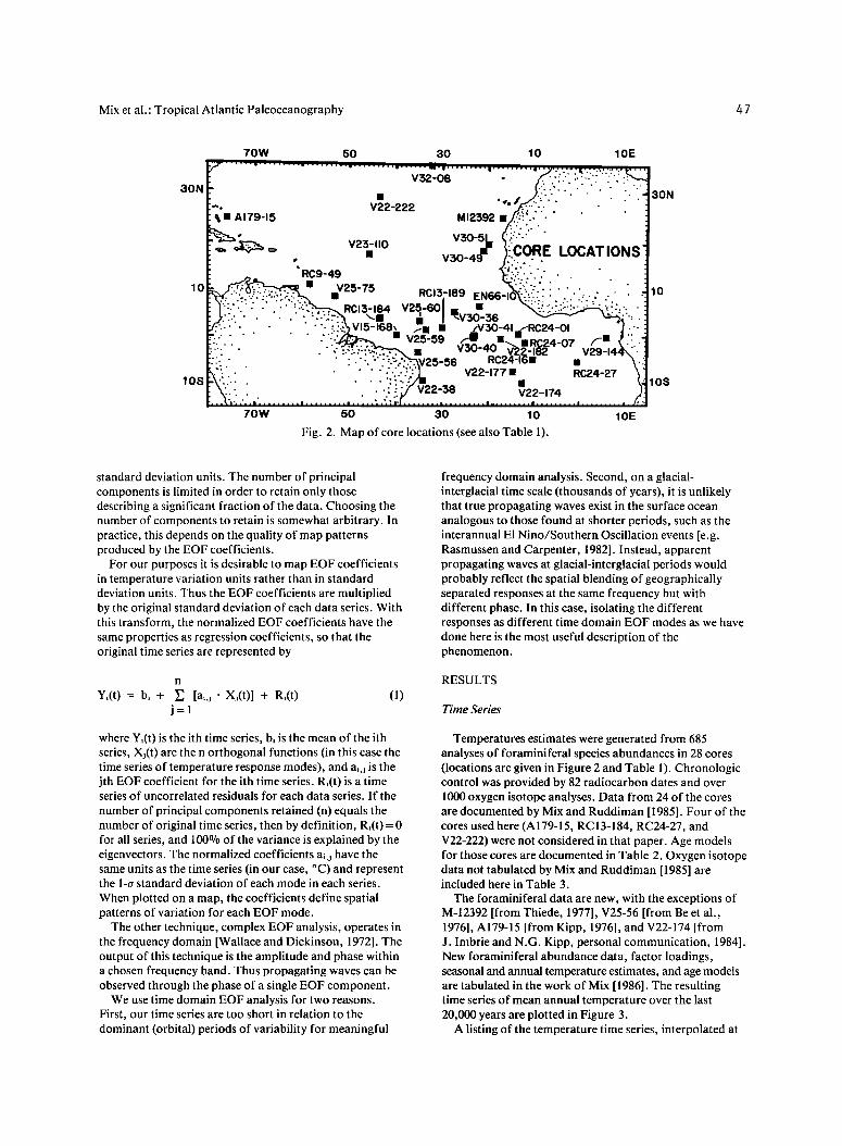
Fig. 2. Map of core locations (see also Table 1).

30N

10

standard deviation units. The number of principal components is limited in order to retain only those describing a significant fraction of the data. Choosing the number of components to retain is somewhat arbitrary. In practice, this depends on the quality of map patterns produced by the EOF coefficients.

For our purposes it is desirable to map EOF coefficients in temperature variation units rather than in standard deviation units. Thus the EOF coefficients are multiplied by the original standard deviation of each data series. With this transform, the normalized EOF coefficients have the same properties as regression coefficients, so that the original time series are represented by

n

Yi(t) = bi + • [ai,j ß Xj(t)] + Ri(t) (1) j--1

where Yi(t) is the ith time series, bi is the mean of the ith series, Xj(t) are the n orthogonal functions (in this case the time series of temperature response modes), and ai,j is the jth EOF coefficient for the ith time series. Ri(t) is a time series of uncorrelated residuals for each data series. If the

number of principal components retained (n) equals the number of original time series, then by definition, Ri(t)= 0 for all series, and 100ø70 of the variance is explained by the eigenvectors. The normalized coefficients ai,j have the same units as the time series (in our case, o C) and represent the 1-a standard deviation of each mode in each series.

When plotted on a map, the coefficients define spatial patterns of variation for each EOF mode.

The other technique, complex EOF analysis, operates in the frequency domain [Wallace and Dickinson, 1972]. The output of this technique is the amplitude and phase within a chosen frequency band. Thus propagating waves can be observed through the phase of a single EOF component.

We use time domain EOF analysis for two reasons. First, our time series are too short in relation to the dominant (orbital) periods of variability for meaningful

frequency domain analysis. Second, on a glacial- interglacial time scale (thousands of years), it is unlikely that true propagating waves exist in the surface ocean analogous to those found at shorter periods, such as the interannual E1Nino/Southern Oscillation events [e.g. Rasmussen and Carpenter, 1982]. Instead, apparent propagating waves at glacial-interglacial periods would probably reflect the spatial blending of geographically separated responses at the same frequency but with different phase. In this case, isolating the different responses as different time domain EOF modes as we have done here is the most useful description of the phenomenon.

RESULTS

Time Series

Temperatures estimates were generated from 685 analyses of foraminiferal species abundances in 28 cores (locations are given in Figure 2 and Table 1). Chronologic control was provided by 82 radiocarbon dates and over 1000 oxygen isotope analyses. Data from 24 of the cores are documented by Mix and Ruddiman [1985]. Four of the cores used here (A179-15, RC13-184, RC24-27, and V22-222) were not considered in that paper. Age models for those cores are documented in Table 2. Oxygen isotope data not tabulated by Mix and Ruddiman [1985] are included here in Table 3.

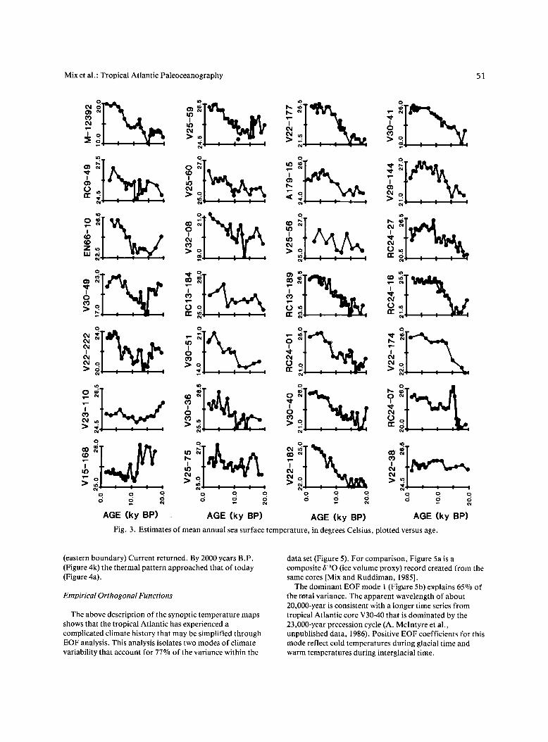
The foraminiferal data are new, with the exceptions of M-12392 [from Thiede, 1977], V25-56 [from Be et at., 1976], A179-15 [from Kipp, 1976], and V22-174 [from J. Imbrie and N.G. Kipp, personal communication, 1984]. New foraminiferal abundance data, factor loadings, seasonal and annual temperature estimates, and age models are tabulated in the work of Mix [1986]. The resulting time series of mean annual temperature over the last 20,000 years are plotted in Figure 3.

A listing of the temperature time series, interpolated at

48 Mix et al.' Tropical Atlantic Paleoceanography

TABLE 1. Core Locations, Depths, and Sedimentation Rates

Core Depth

Latitude Longitude (m)

Mean

Sedimentation

Rate, cm/ky

A179-15

EN66-10G

M-12392

RC9-49

RC13-184

RC13-189

RC24-01

RC24-07

RC24-16

RC24-27

V15-168

V22-38

V22-174

V22-177

V22-182

V22-222

V23-110

V25-56

V25-59

V25-60

V25-75

V29-144

V30-36

V30-40

V30-41K

V30-49

V30-51K

V32-08

24ø48'N 75ø56'W 3109 9.0

6ø39'N 21ø54'W 3527 1.6

25ø10'N 16ø51'W 2575 9.7

11ø11'N 58ø36'W 1851 4.4

3ø52'N 43ø18'W 3446 3.3

1ø52'N 30ø00'W 3233 3.5

0ø34'N 13ø21'W 3850 4.4

1ø21'S 11ø55'W 3899 7.3

5ø02'S 10ø12'W 3543 4.0

5ø25'S 0ø22'W 3718 4.2

0ø12'N 39ø54'W 4219 6.9

9ø33'S 34ø15'W 3797 1.9

10ø04'S 12ø49'W 2630 3.3

7ø45'S 14ø37'W 3290 3.5

0ø33'S 17ø16'W 3776 4.4

28ø56'N 43ø39'W 3197 3.3

17ø38'N 45ø52'W 3746 1.6

3ø33'S 35ø14'W 3512 5.0

1ø22'N 33ø29'W 3824 3.6

3ø17'N 34ø50'W 3749 2.9

8ø35'N 53ø10'W 2743 6.3

0ø12'S 6ø03'E 2685 4.6

5ø21'N 27ø19'W 4245 1.9

0ø12'S 23ø09'W 3706 3.8

0ø13'N 23ø04'W 3874 2.3

18ø26'N 21ø05'W 3093 4.3

19ø52'N 19ø55'W 3409 3.0 34ø47'N 32ø25'W 3252 4.0

2000-year intervals, is in Table 4. Temperature estimates from samples having communalities of less than 0.7 (indicating the possibility of foraminiferal faunas with no exact modern analogue within the calibration data set) are enclosed in parentheses. These values are suspect and should be treated with caution. A complete tabulation of communalities is given by Mix [1986].

Examination of the time series in Figure 3 reveals similarities and differences between the cores. Many records display glacial temperatures (14,000 to 20,000 years B.P.) colder than full interglacial temperatures (0 to 6000 years B.P.). Core V15-168, from the western equatorial Atlantic, records sea surface temperatures warmer in glacial time than in interglacial time. Although this is the only core with this pattern in our data set, it is consistent with the CLIMAP [1981] reconstruction, in which five cores from this area estimated glacial temperatures warmer than at present for one or both seasons. Some of the values older than 14,000 years B.P. in core V15-168, however, have relatively low communali- ties (0.6 to 0.8), reflecting faunal assemblages without a modern analogue. While this does not necessarily mean that the temperature estimates are erroneous, it does suggest caution in their interpretation.

In several of the time series (e.g., RC9-49, V22-222, V23-110, V30-49, and V32-08; see Figure 3) temperature estimates during deglaciation (6000 to 14,000 years B.P.) are as cold or colder than those at the glacial maximum. In addition to these patterns, higher-frequency variability is present in some cores. Significant late Holocene cooling is recorded in cores A179-15, V29-144, V30-49, and V30-51.

Map Patterns

Synoptic map patterns (Figure 4) illustrate the spatial development of tropical sea surface temperatures at 2000-year intervals over the last 20,000 years. Contours were drawn by computer after gridding the data using cubic spline interpolation. Gridding induced some smoothing to the data, within the 1.2øC standard error of the temperature estimates. Final contours were drawn by hand where the data coverage was not sufficient to allow legitimate spline interpolation between data points. In Figure 4, machine-drawn contours are solid, and hand- drawn contours are dashed, indicating uncertainty of exact position.

In the core top map of sites used for downcore study (Figure 4a), the thermal equator (> 26øC) is located

Mix et al.' Tropical Atlantic Paleoceanography /49

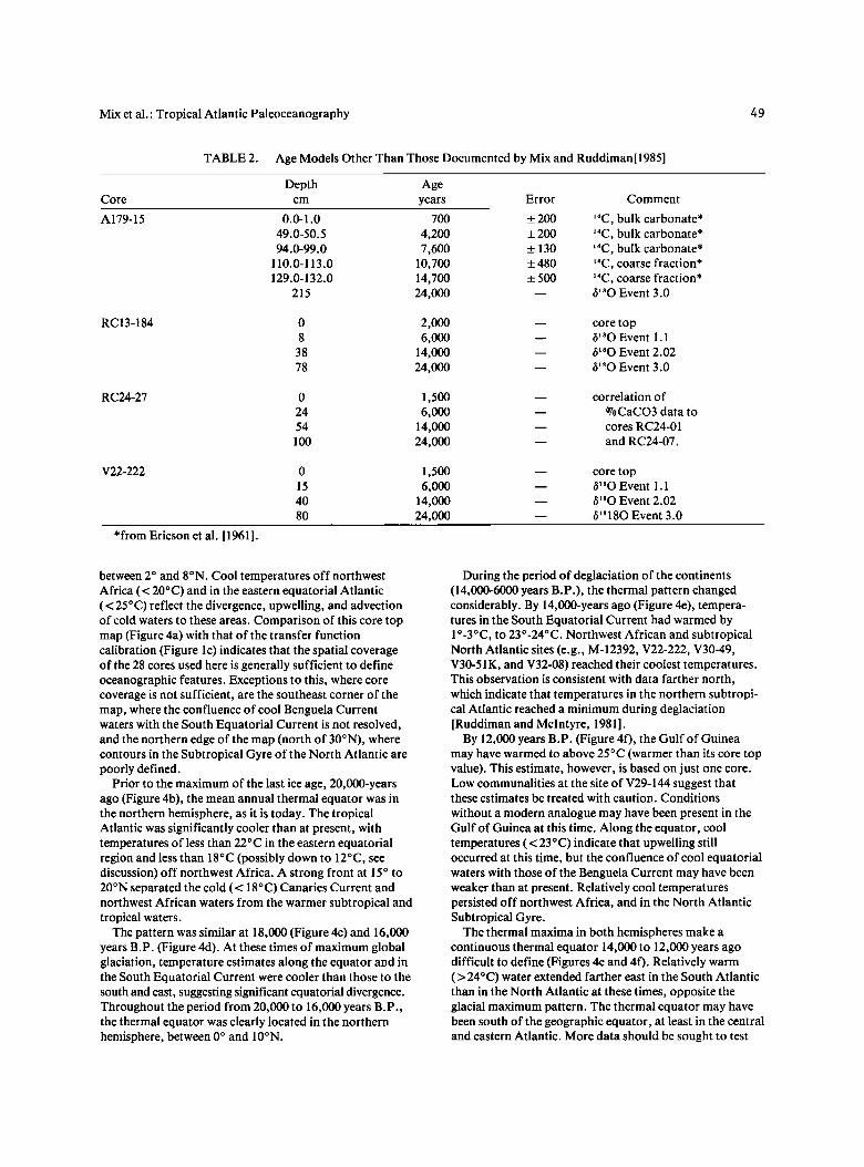
TABLE 2. Age Models Other Than Those Documented by Mix and Ruddiman[1985]

Depth Age Core cm years Error Comment

A179-15

RC13-184

RC24-27

V22-222

0.0-1.0 700 + 200 14C, bulk carbonate* 49.0-50.5 4,200 + 200 14C, bulk carbonate* 94.0-99.0 7,600 + 130 '4C, bulk carbonate*

110.0-113.0 10,700 + 480 '4C, coarse fraction* 129.0-132.0 14,700 + 500 •4C, coarse fraction*

215 24,000 -- r5'80 Event 3.0

0 2,000 -- core top 8 6,000 -- (5•80 Event 1.1

38 14,000 -- (5•O Event 2.02 78 24,000 • (5'•O Event 3.0

0 1,500 • correlation of 24 6,000 -- %CaCO3 data to 54 14,000 -- cores RC24-01 100 24,000 • and RC24-07.

0 1,500 • core top 15 6,000 -- (5•O Event 1.1 40 14,000 -- (5•O Event 2.02 80 24,000 -- (5'8180 Event 3.0

*from Ericson et al. [1961].

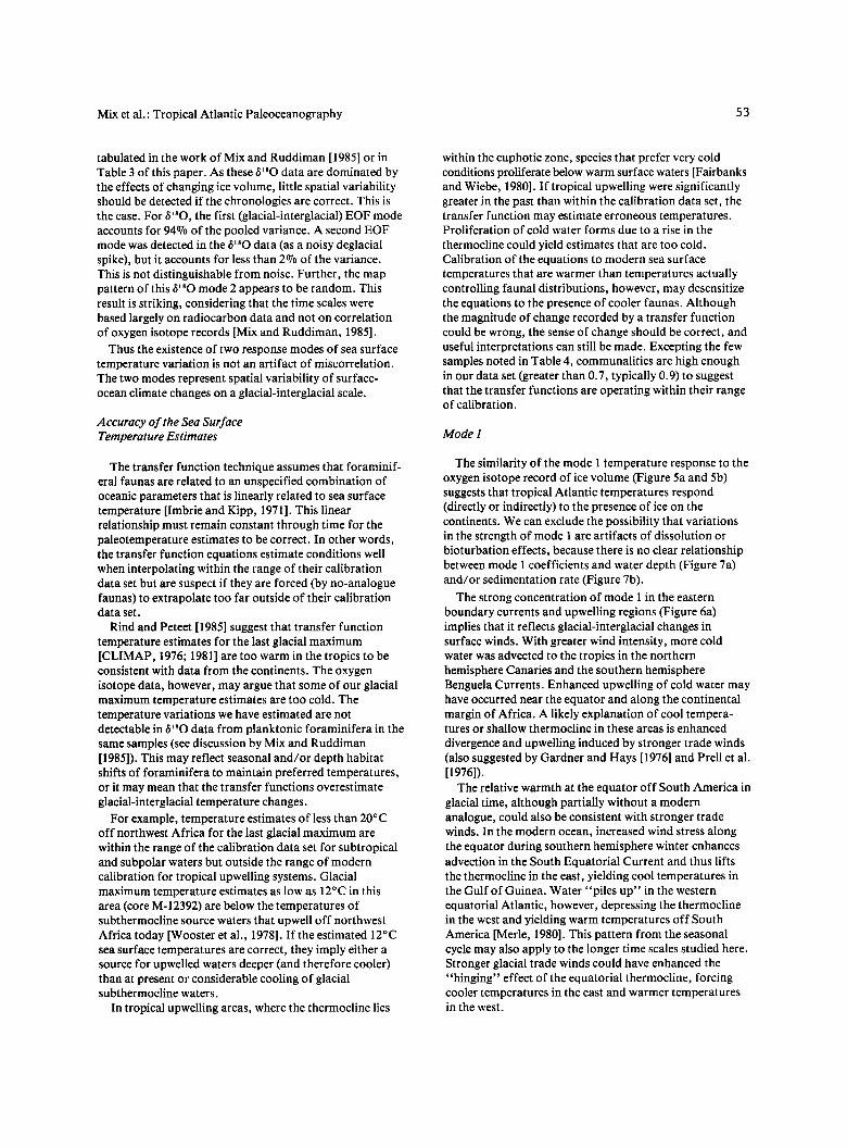
between 2 ø and 8øN. Cool temperatures off northwest Africa ( < 20øC) and in the eastern equatorial Atlantic (< 25øC) reflect the divergence, upwelling, and advection of cold waters to these areas. Comparison of this core top map (Figure 4a) with that of the transfer function calibration (Figure 1 c) indicates that the spatial coverage of the 28 cores used here is generally sufficient to define oceanographic features. Exceptions to this, where core coverage is not sufficient, are the southeast corner of the map, where the confluence of cool Benguela Current waters with the South Equatorial Current is not resolved, and the northern edge of the map (north of 30øN), where contours in the Subtropical Gyre of the North Atlantic are poorly defined.

Prior to the maximum of the last ice age, 20,000-years ago (Figure 4b), the mean annual thermal equator was in the northern hemisphere, as it is today. The tropical Atlantic was significantly cooler than at present, with temperatures of less than 22øC in the eastern equatorial region and less than 18øC (possibly down to 12øC, see discussion) off northwest Africa. A strong front at 15 ø to 20øN separated the cold (< 18øC) Canaries Current and northwest African waters from the warmer subtropical and tropical waters.

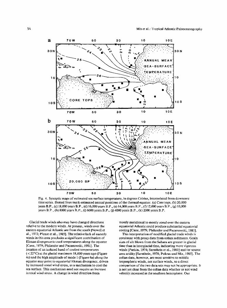
The pattern was similar at 18,000 (Figure 4c) and 16,000 years B.P. (Figure 4d). At these times of maximum global glaciation, temperature estimates along the equator and in the South Equatorial Current were cooler than those to the south and east, suggesting significant equatorial divergence. Throughout the period from 20,000 to 16,000 years B.P., the thermal equator was clearly located in the northern hemisphere, between 0 ø and 10øN.

During the period of deglaciation of the continents (14,000-6000 years B.P.), the thermal pattern changed considerably. By 14,000-years ago (Figure 4e), tempera- tures in the South Equatorial Current had warmed by 1 ø-3øC, to 23ø-24øC. Northwest African and subtropical North Atlantic sites (e.g., M-12392, V22-222, V30-49, V30-51K, and V32-08) reached their coolest temperatures. This observation is consistent with data farther north, which indicate that temperatures in the northern subtropi- cal Atlantic reached a minimum during deglaciation [Ruddiman and Mcintyre, 1981 ].

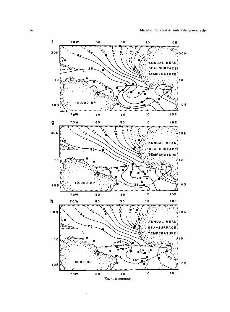
By 12,000 years B.P. (Figure 4f), the Gulf of Guinea may have warmed to above 25øC (warmer than its core top value). This estimate, however, is based on just one core. Low communalities at the site of V29-144 suggest that these estimates be treated with caution. Conditions

without a modern analogue may have been present in the Gulf of Guinea at this time. Along the equator, cool temperatures (< 23øC) indicate that upwelling still occurred at this time, but the confluence of cool equatorial waters with those of the Benguela Current may have been weaker than at present. Relatively cool temperatures persisted off northwest Africa, and in the North Atlantic Subtropical Gyre.

The thermal maxima in both hemispheres make a continuous thermal equator 14,000 to 12,000 years ago difficult to define (Figures 4e and 4f). Relatively warm (> 24øC) water extended farther east in the South Atlantic than in the North Atlantic at these times, opposite the glacial maximum pattern. The thermal equator may have been south of the geographic equator, at least in the central and eastern Atlantic. More data should be sought to test

50 Mix et al.: Tropical Atlantic Paleoceanography

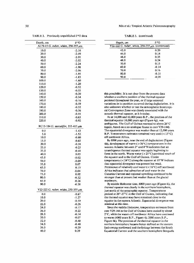
TABLE 3. Previously unpublished 6180 data

Depth, cm b • 80 A179-15 G. ruber, white, 250-355 tan

10.0 -2.16

20.0 -2.09

30.0 -2.01

40.0 -2.02

50.0 -2.24

60.0 -1.98

70.0 -2.06

80.0 -1.95

90.0 -1.83

100.0 -1.60

110.0 -1.20

120.0 -0.52

130.0 -0.55

140.0 -0.20

150.0 -0.34

160.0 -0.16

170.0 -0.59

180.0 -0.52

190.0 -0.56

200.0 -0.55

210.0 -0.63

220.0 -0.92

RC 13-184 G. sacculifer, 355-4 15/am

0.0 -1.43

5.0 -1.52

10.0 -0.80

15.0 -0.65

20.0 -0.38

25.0 -0.25

35.0 -0.41

40.0 0.03

45.0 -0.02

50.0 -0.09

55.0 0.07

65.0 0.13

70.0 -0.04

75.0 0.02

80.0 -0.32

85.0 -0.26

90.0 -0.28

V22-222 G. ruber, white, 250-355/am 0.0 -0.87

10.0 -1.27

20.0 -0.59

22.0 -0.26

24.0 -0.17

26.0 -0.22

28.0 -0.14

30.0 -0.07

32.0 -0.40

34.0 -0.40

36.0 -0.29

40.0 0.29

TABLE 3. (continued)

Depth, cm b • 80 V22-222 G. ruber, white, 250-355/am (continued)

42.0 0.20

44.0 0.14

46.0 0.35

48.0 0.24

50.0 0.15

60.0 -0.14

70.0 0.16

80.0 -0.11

90.0 -0.05

this possibility. It is not clear from the present data whether a southern position of the thermal equator persisted throughout the year, or if large seasonal variations in its position occurred during deglaciation. It is also unknown whether or not the atmospheric Intertropi- cal Convergence Zone was closely associated with the oceanic thermal equator, as it is today.

As at 14,000 and 12,000 years B.P., the position of the thermal equator 10,000 years ago (Figure 4g), was ambiguous. The Gulf of Guinea warmed to above 26øC (again, based on a no-analogue fauna in core V29-144). The equatorial divergence was weaker than at 12,000 years B.P. Temperature estimates remained very cool (< 15øC) off northwest Africa.

By 8000 years ago, near the end of deglaciation (Figure 4h), development of warm (> 26øC) temperatures in the western Atlantic between 2 ø and 8øN indicates that an

unambiguous thermal equator was again beginning to form in the north. Warm water (> 25øC) persisted south of the equator and in the Gulf of Guinea. Cooler temperatures (< 24øC) along the equator at 10øW indicate that equatorial divergence was present but weak. Persistence of relatively cool water ( < 16øC) off northwest Africa indicates that advection of cool water in the

Canaries Current and regional upwelling continued to be stronger than at present but weaker than at the glacial maximum.

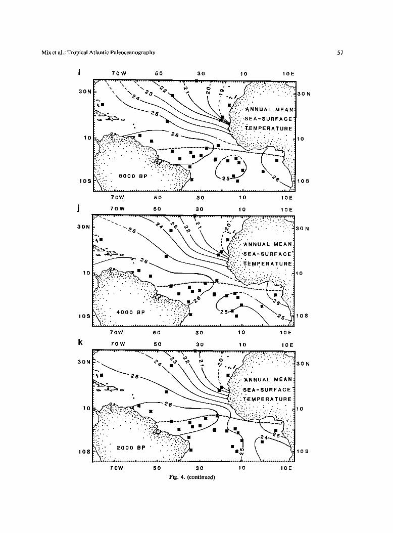
By middle Holocene time, 6000 years ago (Figure 4i), the thermal equator was clearly in the northern hemisphere, just north of the geographic equator. Temperatures peaked at 26ø-27øC in the Gulf of Guinea, indicating that the thermal equator may have remained close to the equator in the eastern Atlantic. Equatorial divergence was minimal at this time.

Since the middle Holocene, temperature estimates from core V29-144 in the Gulf of Guinea have cooled by about 2øC, while the waters off northwest Africa have continued to warm (4000 years B.P., Figure 4j; 2000 years B.P., Figure 4k). The position of the thermal equator in the northern hemisphere became better defined as the eastern limb swung northward and the linkage between the South Equatorial Current and the southern hemisphere Benguela

Mix et al.' Tropical Atlantic Paleoceanography

o. •. • o

• o

o

.

I

O O O O O O O O O O O O

AGE (ky BP) AGE (ky BP) AGE (ky BP) AGE (ky BP) •. 3. •sfimates o• mean annual s•a su•ace tempem[u•e, in dc•ees •dsius, plotted •e•sus a•c.

(eastern boundary) Current returned. By 2000 years B.P. (Figure 4k) the thermal pattern approached that of today (Figure 4a).

Empirical Orthogonal Functions

The above description of the synoptic temperature maps shows that the tropical Atlantic has experienced a complicated climate history that may be simplified through EOF analysis. This analysis isolates two modes of climate variability that account for 77% of the variance within the

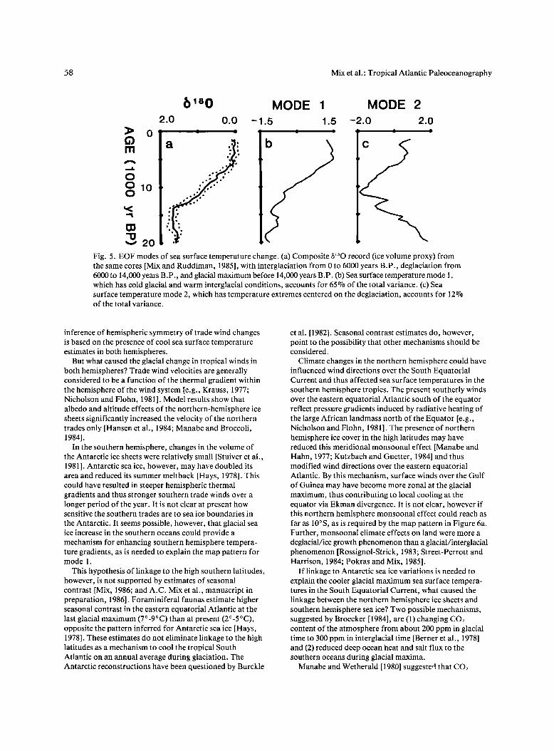
data set (Figure 5). For comparison, Figure 5a is a composite b•80 (ice volume proxy) record created from the same cores [Mix and Ruddiman, 1985].

The dominant EOF mode 1 (Figure 5b) explains 65;% of the't•olal variance. The apparent wavelength of about 20,000-year is consistent with a longer time series from tropical Atlantic core V30•40 that is dominated by the 23,000-year precession cycle (A. Mcintyre et al., unpublished data, 1986). Positive EOF coefficients for this mode reflect cold temperatures during glacial time and warm temperatures during interglacial time.

52 Mix et al.: Tropical Atlantic Paleoceanography

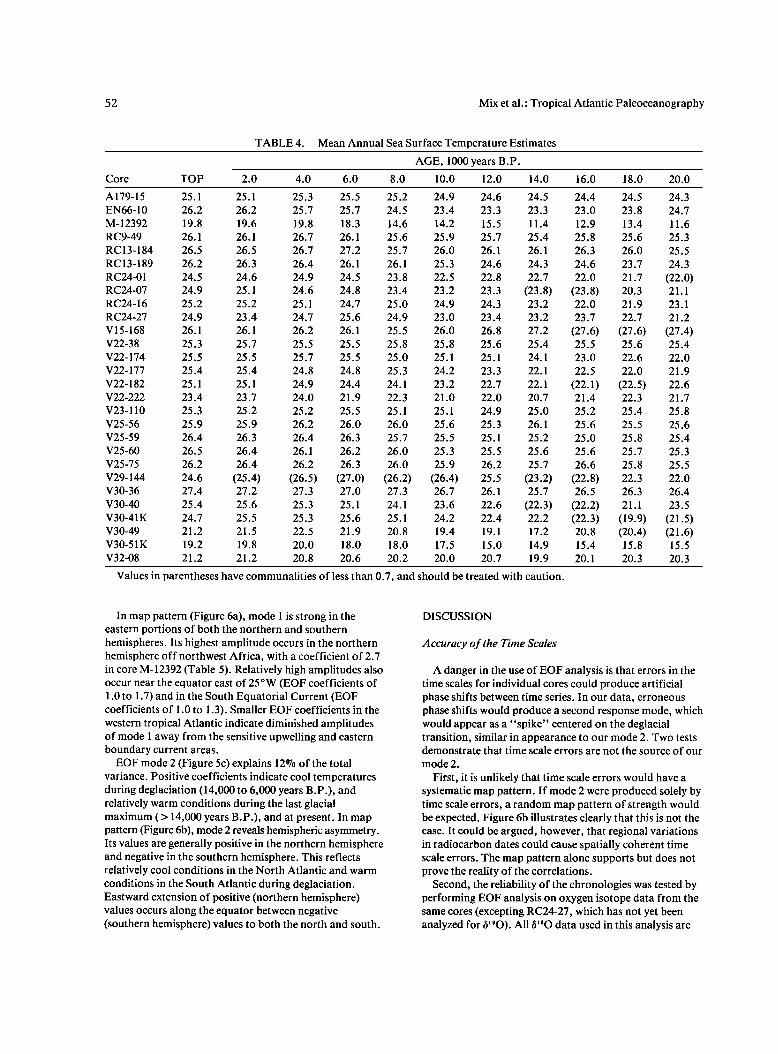
TABLE 4. Mean Annual Sea Surface Temperature Estimates

AGE, 1000 years B.P.

Core TOP 2.0 4.0 6.0 8.0 10.0 12.0 14.0 16.0 18.0 20.0

A179-15 25.1 25.1 25.3 25.5 25.2 24.9 24.6 24.5 24.4 24.5 24.3

EN66-10 26.2 26.2 25.7 25.7 24.5 23.4 23.3 23.3 23.0 23.8 24.7

M-12392 19.8 19.6 19.8 18.3 14.6 14.2 15.5 11.4 12.9 13.4 11.6 RC9-49 26.1 26.1 26.7 26.1 25.6 25.9 25.7 25.4 25.8 25.6 25.3 RC13-184 26.5 26.5 26.7 27.2 25.7 26.0 26.1 26.1 26.3 26.0 25.5

RC13-189 26.2 26.3 26.4 26.1 26.1 25.3 24.6 24.3 24.6 23.7 24.3

RC24-01 24.5 24.6 24.9 24.5 23.8 22.5 22.8 22.7 22.0 21.7 (22.0) RC24-07 24.9 25.1 24.6 24.8 23.4 23.2 23.3 (23.8) (23.8) 20.3 21.1 RC24-16 25.2 25.2 25.1 24.7 25.0 24.9 24.3 23.2 22.0 21.9 23.1 RC24-27 24.9 23.4 24.7 25.6 24.9 23.0 23.4 23.2 23.7 22.7 21.2

V15-168 26.1 26.1 26.2 26.1 25.5 26.0 26.8 27.2 (27.6) (27.6) (27.4) V22-38 25.3 25.7 25.5 25.5 25.8 25.8 25.6 25.4 25.5 25.6 25.4

V22-174 25.5 25.5 25.7 25.5 25.0 25.1 25.1 24.1 23.0 22.6 22.0

V22-177 25.4 25.4 24.8 24.8 25.3 24.2 23.3 22.1 22.5 22.0 21.9

V22-182 25.1 25.1 24.9 24.4 24.1 23.2 22.7 22.1 (22.1) (22.5) 22.6 V22-222 23.4 23.7 24.0 21.9 22.3 21.0 22.0 20.7 21.4 22.3 21.7

V23-110 25.3 25.2 25.2 25.5 25.1 25.1 24.9 25.0 25.2 25.4 25.8

V25-56 25.9 25.9 26.2 26.0 26.0 25.6 25.3 26.1 25.6 25.5 25.6 V25-59 26.4 26.3 26.4 26.3 25.7 25.5 25.1 25.2 25.0 25.8 25.4

V25-60 26.5 26.4 26.1 26.2 26.0 25.3 25.5 25.6 25.6 25.7 25.3 V25-75 26.2 26.4 26.2 26.3 26.0 25.9 26.2 25.7 26.6 25.8 25.5

V29-144 24.6 (25.4) (26.5) (27.0) (26.2) (26.4) 25.5 (23.2) (22.8) 22.3 22.0 V30-36 27.4 27.2 27.3 27.0 27.3 26.7 26.1 25.7 26.5 26.3 26.4

V30-40 25.4 25.6 25.3 25.1 24.1 23.6 22.6 (22.3) (22.2) 21.1 23.5 V30-41K 24.7 25.5 25.3 25.6 25.1 24.2 22.4 22.2 (22.3) (19.9) (21.5) V30-49 21.2 21.5 22.5 21.9 20.8 19.4 19.1 17.2 20.8 (20.4) (21.6) V30-51K 19.2 19.8 20.0 18.0 18.0 17.5 15.0 14.9 15.4 15.8 15.5

V32-08 21.2 21.2 20.8 20.6 20.2 20.0 20.7 19.9 20.1 20.3 20.3

Values in parentheses have communalities of less than 0.7, and should be treated with caution.

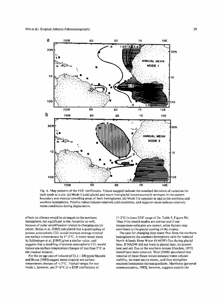
In map pattern (Figure 6a), mode 1 is strong in the eastern portions of both the northern and southern hemispheres. Its highest amplitude occurs in the northern hemisphere off northwest Africa, with a coefficient of 2.7 in core M-12392 (Table 5). Relatively high amplitudes also occur near the equator east of 25øW (EOF coefficients of 1.0 to 1.7) and in the South Equatorial Current (EOF coefficients of 1.0 to 1.3). Smaller EOF coefficients in the western tropical Atlantic indicate diminished amplitudes of mode 1 away from the sensitive upwelling and eastern boundary current areas.

EOF mode 2 (Figure 5c) explains 12070 of the total variance. Positive coefficients indicate cool temperatures during deglaciation (14,000 to 6,000 years B.P.), and relatively warm conditions during the last glacial maximum (> 14,000 years B.P.), and at present. In map pattern (Figure 6b), mode 2 reveals hemispheric asymmetry. Its values are generally positive in the northern hemisphere and negative in the southern hemisphere. This reflects relatively cool conditions in the North Atlantic and warm conditions in the South Atlantic during deglaciation. Eastward extension of positive (northern hemisphere) values occurs along the equator between negative (southern hemisphere) values to both the north and south.

DISCUSSION

Accuracy of the Time Scales

A danger in the use of EOF analysis is that errors in the time scales for individual cores could produce artificial phase shifts between time series. In our data, erroneous phase shifts would produce a second response mode, which would appear as a "spike" centered on the deglacial transition, similar in appearance to our mode 2. Two tests demonstrate that time scale errors are not the source of our mode 2.

First, it is unlikely that time scale errors would have a systematic map pattern. If mode 2 were produced solely by time scale errors, a random map pattern of strength would be expected. Figure 6b illustrates clearly that this is not the case. It could be argued, however, that regional variations in radiocarbon dates could cause spatially coherent time scale errors. The map pattern alone supports but does not prove the reality of the correlations.

Second, the reliability of the chronologies was tested by performing EOF analysis on oxygen isotope data from the same cores (excepting RC24-27, which has not yet been analyzed for •i180). All •i180 data used in this analysis are

Mix et al.: Tropical Atlantic Paleoceanography 5 3

tabulated in the work of Mix and Ruddiman [ 1985] or in Table 3 of this paper. As these b•80 data are dominated by the effects of changing ice volume, little spatial variability should be detected if the chronologies are correct. This is the case. For b'80, the first (glacial-interglacial) EOF mode accounts for 94ø7o of the pooled variance. A second EOF mode was detected in the •80 data (as a noisy deglacial spike), but it accounts for less than 2ø7o of the variance. This is not distinguishable from noise. Further, the map pattern of this •80 mode 2 appears to be random. This result is striking, considering that the time scales were based largely on radiocarbon data and not on correlation of oxygen isotope records [Mix and Ruddiman, 1985].

Thus the existence of two response modes of sea surface temperature variation is not an artifact of miscorrelation. The two modes represent spatial variability of surface- ocean climate changes on a glacial-interglacial scale.

Accuracy of the Sea Surface Temperature Estimates

The transfer function technique assumes that foraminif- eral faunas are related to an unspecified combination of oceanic parameters that is linearly related to sea surface temperature [Imbrie and Kipp, 1971 ]. This linear relationship must remain constant through time for the paleotemperature estimates to be correct. In other words, the transfer function equations estimate conditions well when interpolating within the range of their calibration data set but are suspect if they are forced (by no-analogue faunas) to extrapolate too far outside of their calibration data set.

Rind and Peteet [1985] suggest that transfer function temperature estimates for the last glacial maximum [CLIMAP, 1976; 1981] are too warm in the tropics to be consistent with data from the continents. The oxygen isotope data, however, may argue that some of our glacial maximum temperature estimates are too cold. The temperature variations we have estimated are not detectable in •'80 data from planktonic foraminifera in the same samples (see discussion by Mix and Ruddiman [1985]). This may reflect seasonal and/or depth habitat shifts of foraminifera to maintain preferred temperatures, or it may mean that the transfer functions overestimate glacial-interglacial temperature changes.

For example, temperature estimates of less than 20øC off northwest Africa for the last glacial maximum are within the range of the calibration data set for subtropical and subpolar waters but outside the range of modern calibration for tropical upwelling systems. Glacial maximum temperature estimates as low as 12øC in this area (core M-12392) are below the temperatures of subthermocline source waters that upwell off northwest Africa today [Wooster et al., 1978]. If the estimated 12øC sea surface temperatures are correct, they imply either a source for upwelled waters deeper (and therefore cooler) than at present or considerable cooling of glacial subthermocline waters.

In tropical upwelling areas, where the thermocline lies

within the euphotic zone, species that prefer very cold conditions proliferate below warm surface waters [Fairbanks and Wiebe, 1980]. If tropical upwelling were significantly greater in the past than within the calibration data set, the transfer function may estimate erroneous temperatures. Proliferation of cold water forms due to a rise in the

thermocline could yield estimates that are too cold. Calibration of the equations to modern sea surface temperatures that are warmer than temperatures actually controlling faunal distributions, however, may desensitize the equations to the presence of cooler faunas. Although the magnitude of change recorded by a transfer function could be wrong, the sense of change should be correct, and useful interpretations can still be made. Excepting the few samples noted in Table 4, communalities are high enough in our data set (greater than 0.7, typically 0.9) to suggest that the transfer functions are operating within their range of calibration.

Mode 1

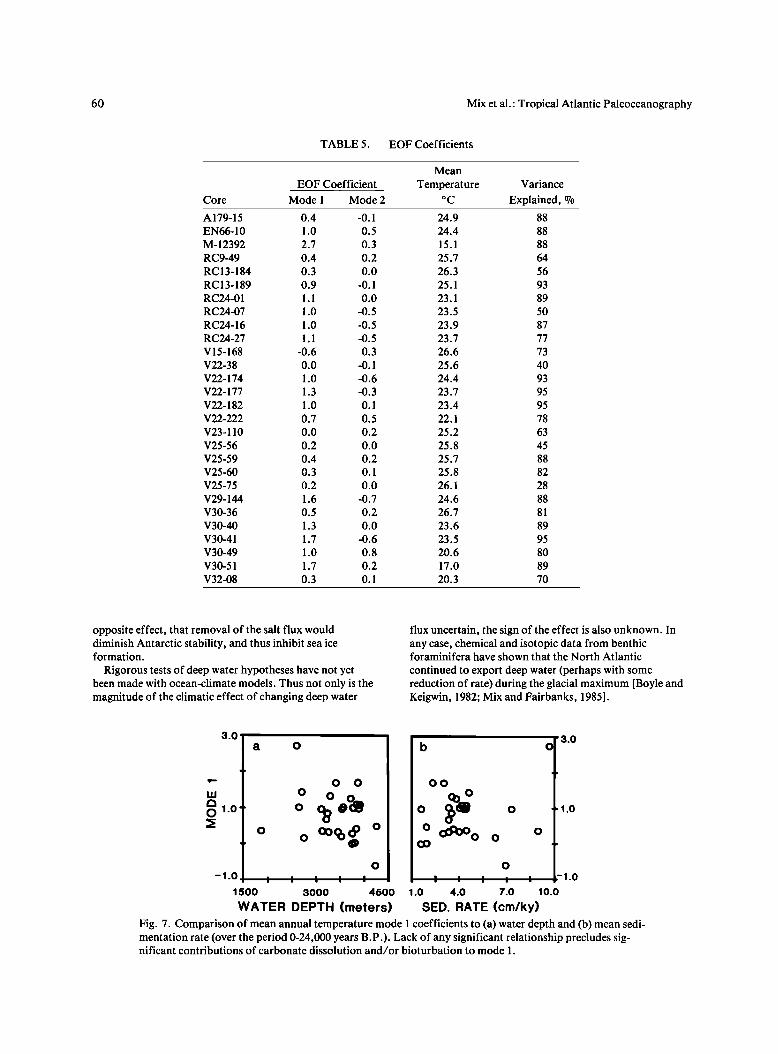
The similarity of the mode 1 temperature response to the oxygen isotope record of ice volume (Figure 5a and 5b) suggests that tropical Atlantic temperatures respond (directly or indirectly) to the presence of ice on the continents. We can exclude the possibility that variations in the strength of mode 1 are artifacts of dissolution or bioturbation effects, because there is no clear relationship between mode 1 coefficients and water depth (Figure 7a) and/or sedimentation rate (Figure 7b).

The strong concentration of mode 1 in the eastern boundary currents and upwelling regions (Figure 6a) implies that it reflects glacial-interglacial changes in surface winds. With greater wind intensity, more cold water was advected to the tropics in the northern hemisphere Canaries and the southern hemisphere Benguela Currents. Enhanced upwelling of cold water may have occurred near the equator and along the continental margin of Africa. A likely explanation of cool tempera- tures or shallow thermocline in these areas is enhanced

divergence and upwelling induced by stronger trade winds (also suggested by Gardner and Hays [1976] and Prell et al. [1976]).

The relative warmth at the equator off South America in glacial time, although partially without a modern analogue, could also be consistent with stronger trade winds. In the modern ocean, increased wind stress along the equator during southern hemisphere winter enhances advection in the South Equatorial Current and thus lifts the thermocline in the east, yielding cool temperatures in the Gulf of Guinea. Water "piles up" in the western equatorial Atlantic, however, depressing the thermocline in the west and yielding warm temperatures off South America [Merle, 1980]. This pattern from the seasonal cycle may also apply to the longer time scales studied here. Stronger glacial trade winds could have enhanced the "hinging" effect of the equatorial thermocline, forcing cooler temperatures in the east and warmer temperatures in the west.

54 Mix et at.: Tropical Atlantic Paleoceanography

a 70W 50 30 10 10E

• ß • • ............ ß ..... s - .....: .... . ...'.:... 30N ;"K ........... '• ......... •'k' "•' [] '1' "• ......... ",:4':'.'"."':•.":":"!".'".'q.UE % O '- o "?'"'' "" ' ''":"-•30 N ,, [] , ,::•".'.' . :

• , m .'.:: .' ß - •25 ,• :'.'.. 'A. NNUAL MEAN: [ •--" '•, A- SURF A C E'" . • -•_•'5/i•';: •-E M PER A TURE!

--'2 6 [] :.i' ::.: ::.:.,'-.-'..' .' ".'-

.................................. i .................. ":."-';':':"::"' '" "L: :,::...' = [] _-- . ..'.::

[] []

10S 10S ............... ß '-.;'. •' , , ,• f-.: t

70W 50 30 10 10E

b 70W 50 30 10 10E

x•,•'•o, ,.,,.,• ,,, o, )' ' •o • • /.• :'..: : . • !;!."!' ' .. 30N • ,... i ?' I,,7. I / . )/:'-'. ''. 30 N • • il•'•'.•x•...'-.\-

'i, [] •m '?.•..'" ' [-;- [ ̂ - s u, ^ c [

'"" • ".".':'..:-i :. •,..': ' . ' - I 0 = ...... ' ..... '-i ";-'.'" :.'.'.: .'..".' .' ß I 0

ß ......... i• / ' ':.".':.•' ;.::': :"'" .... ::::':' ' • ..o:.: ?. 6 -"'m ß 1• [] '?."' ...' [] ......

105 'lOS

70W 50 30 10 10E

Fig. 4. Synoptic maps of estimated sea surface temperature, in degrees Celsius, interpolated from downcore time series. Dotted lines mark estimated annual positions of the thermal equator. (a) Core tops, (b) 20,000 years B.P., (c) 18,000 years B.P., (d) 16,000 years B.P., (e) 14,000 years B.P., (f) 12,000 years B.P., (g) 10,000 years B.P., (h) 8000 years B.P., (i) 6000 years B.P., (j) 4000 years B.P., (k) 2000 years B.P.

Glacial trade winds also may have changed directions relative to the modern winds. At present, winds over the eastern equatorial Atlantic are from the south [Newell et al., 1972; Picaut et al., 1985]. The relative lack of easterly winds in this area precludes a significant contribution of Ekman divergence to cool temperatures along the equator [Cane, 1979; Philander and Pacanowski, 1981]. The location of an isolated band of coolest temperatures (< 22øC) at the glacial maximum 18,000 years ago (Figure 4c) and the high amplitude of mode 1 (Figure 6a) along the equator may point to equatorial Ekman divergence, driven by increased zonal wind stress, as a mechanism to cool the sea surface. This mechanism need not require an increase in total wind stress. A change in wind direction from

mostly meridional to mostly zonal over the eastern equatorial Atlantic could produce substantial equatorial cooling [Cane, 1979; Philander and Pacanowski, 1981].

This interpretation of modified glacial trade winds is consistent with proxy data from eolian sediments. Grain sizes of silt blown from the Sahara are greater in glacial time than in interglacial time, indicating more vigorous winds [Parkin, 1974; Sarnthein et at., 1981] and/or source area aridity [Sarnthein, 1978; Pokras and Mix, 1985]. The eolian data, however, are most sensitive to middle tropospheric winds, not surface winds, so a direct comparison of the two data sets may not be appropriate. It is not yet clear from the eolian data whether or not wind velocity increased in the southern hemisphere. Our

Mix et al.' Tropical Atlantic Paleoceanography 55

C 70w 50 30 10 10E

30N ,'-- ,,. / , '.'.'."-.' . ß ' ''..'.:; [' • %.• x , ' :, ,',.,, ,•..:•":'. . . ..:•o,,,. \ ! I I ",::"'"' ' ' •.m \\ •1 [] .'.::.'.. ß :

lO ' :'.:'.::-'.'. :'- ' .: i.' .. ' : •o [] ........... ".}.".: '.L :...'.'.''-'..' ':

......._-.= • •...i ........ ....... .... ... •..-•.!...:: ! ?.."f...- ... _. _ -.•_ [] '.::::' J

10S 108

70W ,50 3,0 10 10E

d 7ow ,50 3,0 lO lOE

:"F-'. ...... ...... g ........ r"'"l"g 3ON[- •,,,. '"'7%' •"•-- •""'\ • ; • '""" fl ):i'"_"""' ' ' :''.".•30N

[:..... e½._ '•. %. \ \ • ,,,, ;'.'..•/..'-.'." -: \ 't % • ,'.' '' ' ' •'[] x\ \ % I[] '"::'.i' ' : 25 ":':'"

[• ' _ • -'""'-•••"•'i.:,': 1 'T.E M P E R A T U R E i

, • '.".':".'.:.::.i;;.'.' ß i i. ,o •.... ..... [] • ' o-.., .:

27" [] - -- X ""-

ß .-" i• [] <• •:.'.:: -_' ß . , :.-:.'3:"..'L... [] '":'.. !

lOS "'" ' ß . .. v..:..'..,. [] m ':!11 lOS 70W 50 30 10 10E

e 70W 50 30 10 10E

% '"' '"' • ":' /,,' ..:..':":i'::•'::".'.'". '.':.:'.':• ,,t. "' I I "-/,

E"' '"3. \ \ •\ I tl, '.'.'A, NNUAL MEAN

m ".:.':'..:-: :. :...': ' ß ' ß I 0 m ".:•::-'.. ':.: .'.,.:.,'..".' .'

26 .... '• .......... '• ......... '::.i.::::.::'i::": ..... :!:,'.' ' : ..... . ...... [] '[] ß . 23•....•-:•:: ........... [] im [] [] []

.... ?o ooOø' o..o

ß '•'.' ' 14 000 BP, ' ' ':.':.':..:),'• .... •,, .....

70W 50 30 10 10E

Fig. 4. (continued)

30N

10

10S

56 Mix et al.: Tropical Atlantic Paleoceanography

f 70 w 50 30 10 10E

30N ';'•'."'.' .' ' ' '".':"::30 N

•o [] :'•:::.:-'.'-i.".'.:.::...: •o

10S 10S

70W 50 30 10 10E

g 70W 50 30 10 10E ..... • •, ...... ".:• ........... "•= .......... ='I'"•"i"1""; ..... "'•. ':."Y:'..'-'..':".'.'::.':';•: ß . .'"•_ ,.,.. • -..,,,,• ":•:..:.......-.:..:::....• 30m • • '" o •o t T " '-'.'.''.' ß ' ''."'-; N • I / '. • •-o ..... . . '.:30 ß ,-, ,e• • \ • t ,.;:•".'.' ß : ß ',,'• •:::.':.:"^,, u ̂,

A-SURFACE'.'

[ '• ••'•,•'••.'•'.-'i:.::: .• .E M P E R A T U R E i

o ...-....<. ..,.. . .....• '"'"]•'.•:.:.:-:'..'.: i: :. ' ] • o I [] ".'.v-.: '.L :....: .'.' ß-' .- . ' ':

'.: ......... -- [] [] •,e5 .'.'.': 24 'i ' ("'•

•..•ii i,',i i i ' !::'::'.•i'. ............. ,o• ,?,.., ...... •.- ..... ..:,..•..:i!!:•i•.: .... iii::':•::!: ,• -•i 70W 50 30 10 10E

h 70w 50 30 10 10E

. ".• -% • • •,, • , '::.....-..:......::.... ," 0 j ,'-• ,, ,,

, ß 'ANNUAL MEAN

30N

10

10S

X• • • III .'.?'." i'.:".'.'"S E A- SURF ACE'

', +EMp. ERATURE I ....•'•__•, • ••.'-•:'..•-;.-.:... : '. '.. :

..... ': :.....,...:•,::.. ,•..• ••i.'-.'-...:....:•.:-::.-'•::...: ............. ' '"•' • ......... I'"?"'?'-=A ..... .,•..'::. ;:.:'. '. ß ß ß :.L;"x• ß J -L•.• / .... ,t•"'-•.:'.":i.; :•i-:.i•'.'- ."•:•:•/.-:.':'.:. "-.-..•,---? LL -, ........ •;" •,•.•:• •':" ' 8 ' '. '..' '-":"':"." ...... 25 [] ...-"' • '.: ß . - 000 BP ' "..'-.' ............ .. .. . ..... : .......... ?.. • •

70W 50 30 10 10E

Fig. 4. (continued)

30N

10

10S

Mix et al.' Tropical Atlantic Paleoceanography 5 7

k

30N

10

10S

Fig. 4. (continued)

58 Mix et al.: Tropical Atlantic Paleoceanography

b180 MODE I MODE 2

o10 o

• 80

2.0 0.0 -1.5 1.5 -2.0 2.0

C

Fig. 5. EOF modes of sea surface temperature change. (a) Composite •80 record (ice volume proxy) from the same cores [Mix and Ruddiman, 1985], with interglaciation from 0 to 6000 years B.P., deglaciation from 6000 to 14,000 years B.P., and glacial maximum before 14,000 years B.P. (b) Sea surface temperature mode 1, which has cold glacial and warm interglacial conditions, accounts for 65 ø70 of the total variance. (c) Sea surface temperature mode 2, which has temperature extremes centered on the deglaciation, accounts for 12ø70 of the total variance.

inference of hemispheric symmetry of trade wind changes is based on the presence of cool sea surface temperature estimates in both hemispheres.

But what caused the glacial change in tropical winds in both hemispheres? Trade wind velocities are generally considered to be a function of the thermal gradient within the hemisphere of the wind system [e.g., Krauss, 1977; Nicholson and Flohn, 1981]. Model results show that albedo and altitude effects of the northern-hemisphere ice sheets significantly increased the velocity of the northern trades only [Hansen et al., 1984; Manabe and Broccoli, 1984].

In the southern hemisphere, changes in the volume of the Antarctic ice sheets were relatively small [Stuiver et al., 1981]. Antarctic sea ice, however, may have doubled its area and reduced its summer meltback [Hays, 1978]. This could have resulted in steeper hemispheric thermal gradients and thus stronger southern trade winds over a longer period of the year. It is not clear at present how sensitive the southern trades are to sea ice boundaries in

the Antarctic. It seems possible, however, that glacial sea ice increase in the southern oceans could provide a mechanism for enhancing southern hemisphere tempera- ture gradients, as is needed to explain the map pattern for mode 1.

This hypothesis of linkage to the high southern latitudes, however, is not supported by estimates of seasonal contrast [Mix, 1986; and A.C. Mix et al., manuscript in preparation, 1986]. Foraminiferal faunas estimate higher seasonal contrast in the eastern equatorial Atlantic at the last glacial maximum (7ø-9øC) than at present (2ø-5øC), opposite the pattern inferred for Antarctic sea ice [Hays, 1978]. These estimates do not eliminate linkage to the high latitudes as a mechanism to cool the tropical South Atlantic on an annual average during glaciation. The Antarctic reconstructions have been questioned by Burckle

et al. [1982]. Seasonal contrast estimates do, however, point to the possibility that other mechanisms should be considered.

Climate changes in the northern hemisphere could have influenced wind directions over the South Equatorial Current and thus affected sea surface temperatures in the southern hemisphere tropics. The present southerly winds over the eastern equatorial Atlantic south of the equator reflect pressure gradients induced by radiative heating of the large African landmass north of the Equator [e.g., Nicholson and Flohn, 1981]. The presence of northern hemisphere ice cover in the high latitudes may have reduced this meridional monsoonal effect [Manabe and Hahn, 1977; Kutzbach and Guetter, 1984] and thus modified wind directions over the eastern equatorial Atlantic. By this mechanism, surface winds over the Gulf of Guinea may have become more zonal at the glacial maximum, thus contributing to local cooling at the equator via Ekman divergence. It is not clear, however if this northern hemisphere monsoonal effect could reach as far as 10øS, as is required by the map pattern in Figure 6a. Further, monsoonal climate effects on land were more a deglacial/ice growth phenomenon than a glacial/interglacial phenomenon [Rossignol-Strick, 1983; Street-Perrott and Harrison, 1984; Pokras and Mix, 1985].

If linkage to Antarctic sea ice variations is needed to explain the cooler glacial maximum sea surface tempera- tures in the South Equatorial Current, what caused the linkage between the northern hemisphere ice sheets and southern hemisphere sea ice? Two possible mechanisms, suggested by Broecker [1984], are (1) changing CO2 content of the atmosphere from about 200 ppm in glacial time to 300 ppm in interglacial time [Berner et al., 1978] and (2) reduced deep ocean heat and salt flux to the southern oceans during glacial maxima.

Manabe and Wetheraid [1980] suggeste4 that CO2

Mix et al ß Tropical Atlantic Paleoceanography 59

a 70w

30N

10

10S

70W

70W

ß . ß

ß

ß

50

.5

30 10 10E

1.0-==1

ß ß 30N • . .

..

ß .

'ANNUAL MEAN

MODE 1 ..

ß

ß

....

. . .

ß . .. ß

.5

10

50 30 10 10E

50 30 10 10E

10S

30N

10

ß

ß , ß ,

ß

'. ßANNUAL MEAN ,..

', '. MODE 2 ß

ß ß .

,

10S ' '.'..'." 10S ß

70W 50 30 10 10E

Fig. 6. Map patterns of the EOF coefficientsß Values mapped indicate the standard deviation of variation for each mode at a site. (a) Mode 1 (cold glacial and warm interglacial temperatures) is strongest in the eastern boundary and tropical upwelling areas of both hemispheres. (b) Mode 2 is opposite in sign in the northern and southern hemispheres. Positive values indicate relatively cold conditions, and negative values indicate relatively warm conditions during deglaciation.

effects on climate would be strongest in the northern hemisphere, but significant in the Antarctic as well, because of polar amplification related to changing sea ice extent. Bryan et al. [1982] calculated that a quadrupling of present atmospheric CO2 would increase average tropical sea-surface temperatures by 1 ø-2ø(2. A more recent study by Schlesinger et al. [1985] gives a similar value, and suggests that a doubling of present atmospheric CO2 would induce sea-surface temperature changes of less than 2ø(2 in the tropical Atlantic.

For the ice-age case of reduced pCO2 (--- 200 ppm) Manabe and Bryan [1985] suggest mean tropical sea surface temperature changes of < 2øC. Typical ranges for our mode 1, however, are 3ø-6ø(2 (1-t• EOF coefficients of

1 ø-2øC/a times EOF range of 3a; Table 5, Figure 5b). Thus if the model studies are correct and if our

temperature estimates are correct, other factors may contribute to the glacial cooling of the tropics.

The case for changing deep water flux from the northern hemisphere to the southern hemisphere calls for reduced North Atlantic Deep Water (NADW) flux during glacial time. If NADW did not form in glacial time, its present heat and salt flux to the southern oceans [Gordon, 1975] would have been removed. Weyl [1968] speculated that removal of these fluxes would enhance water column

stability, increase sea ice extent, and thus strengthen southern hemisphere thermal gradients. Martinson [personal communication, 1985], however, suggests exactly the

60 Mix et al.: Tropical Atlantic Paleoceanography

TABLE 5. EOF Coefficients

EOF Coefficient

Core Mode 1 Mode 2

A179-15 0.4 -0.1

EN66-10 1.0 0.5

M-12392 2.7 0.3

RC9-49 0.4 0.2

RC13-184 0.3 0.0

RC13-189 0.9 -0.1

RC24-01 1.1 0.0

RC24-07 1.0 -0.5

RC24-16 1.0 -0.5

RC24-27 1.1 -0.5

V15-168 -0.6 0.3

V22-38 0.0 -0.1

V22-174 1.0 -0.6

V22-177 1.3 -0.3

V22-182 1.0 0.1

V22-222 0.7 0.5

V23-110 0.0 0.2

V25-56 0.2 0.0

V25o59 0.4 0.2

V25-60 0.3 0.1

V25-75 0.2 0.0

V29-144 1.6 -0.7

V30-36 0.5 0.2

V30-40 1.3 0.0

V30-41 1.7 -0.6

V30-49 1.0 0.8

V30-51 1.7 0.2

V32-08 0.3 0.1

Mean

Temperature øC

Variance

Explained, ø7o

24.9 88

24.4 88

15.1 88

25.7 64

26.3 56

25.1 93

23.1 89

23.5 50

23.9 87

23.7 77

26.6 73

25.6 40

24.4 93

23.7 95

23.4 95

22.1 78

25.2 63

25.8 45

25.7 88

25.8 82

26.1 28

24.6 88

26.7 81

23.6 89

23.5 95

20.6 80

17.0 89

20.3 70

opposite effect, that removal of the salt flux would diminish Antarctic stability, and thus inhibit sea ice formation.

Rigorous tests of deep water hypotheses have not yet been made with ocean-climate models. Thus not only is the magnitude of the climatic effect of changing deep water

flux uncertain, the sign of the effect is also unknown. In any case, chemical and isotopic data from benthic foraminifera have shown that the North Atlantic

continued to export deep water (perhaps with some reduction of rate) during the glacial maximum [Boyle and Keigwin, 1982; Mix and Fairbanks, 1985].

3.0 L

0 1.0 0

-1.0 ; 1500

0 0

o o o

ß ß ß

3000 4500

WATER DEPTH (meters)

73.0 b o

oo

Cb o

o o 0 •0 0 0

0

ß ß ß i I -1.0 1.0 4.0 7.0 10.0

SED. RATE (cm/ky) Fig. 7. Comparison of mean annual temperature mode 1 coefficients to (a) water depth and (b) mean sedi- mentation rate (over the period 0-24,000 years B.P.). Lack of any significant relationship precludes sig- nificant contributions of carbonate dissolution and/or bioturbation to mode 1.

Mix et al.: Tropical Atlantic Paleoceanography 6 !

1.0

• 0.0 o

a

-1.0

1500

0

o o o o

o ø o o

b o

o o o

3000 4500 1.0 7.0

WATER DEPTH (meters)

o

o o o

4.0

1.0

o o.o

-1 .o i -

lO.O

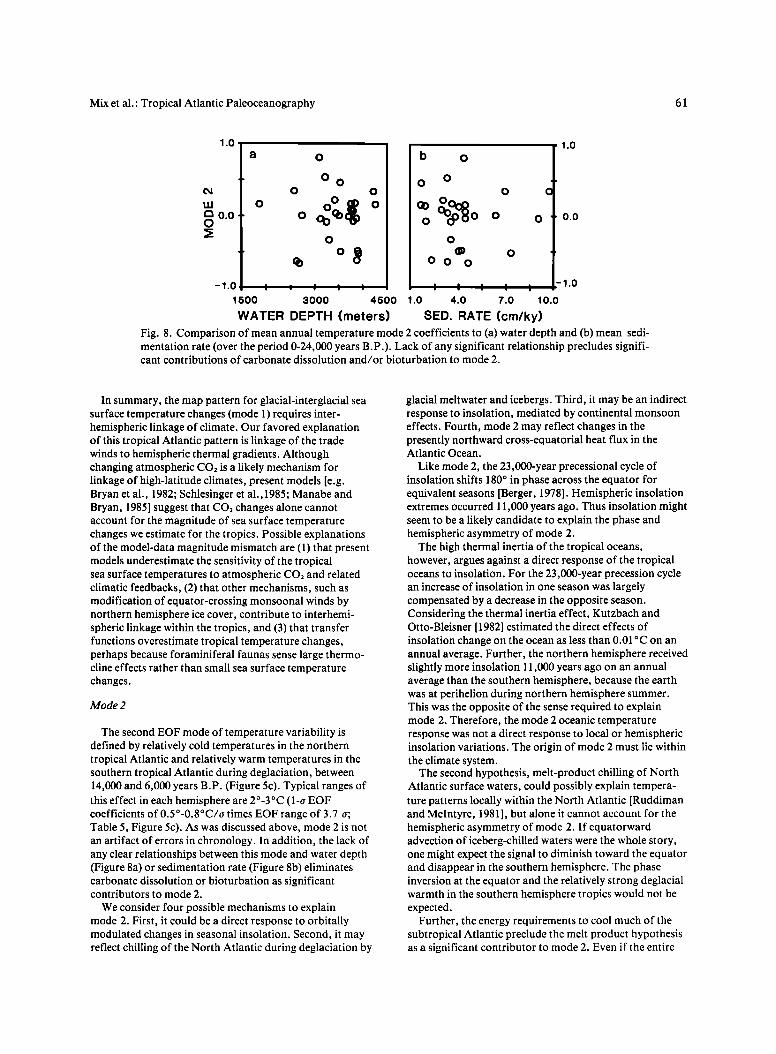
SED. RATE (cm/ky) Fig. 8. Comparison of mean annual temperature mode 2 coefficients to (a) water depth and (b) mean sedi- mentation rate (over the period 0-24,000 years B.P.). Lack of any significant relationship precludes signifi- cant contributions of carbonate dissolution and/or bioturbation to mode 2.

In summary, the map pattern for glacial-interglacial sea surface temperature changes (mode 1) requires inter- hemispheric linkage of climate. Our favored explanation of this tropical Atlantic pattern is linkage of the trade winds to hemispheric thermal gradients. Although changing atmospheric CO2 is a likely mechanism for linkage of high-latitude climates, present models [e.g. Bryan et al., 1982; Schlesinger et a1.,1985; Manabe and Bryan, 1985] suggest that CO2 changes alone cannot account for the magnitude of sea surface temperature changes we estimate for the tropics. Possible explanations of the model-data magnitude mismatch are (1) that present models underestimate the sensitivity of the tropical sea surface temperatures to atmospheric CO• and related climatic feedbacks, (2) that other mechanisms, such as modification of equator-crossing monsoonal winds by northern hemisphere ice cover, contribute to interhemi- spheric linkage within the tropics, and (3) that transfer functions overestimate tropical temperature changes, perhaps because foraminiferal faunas sense large thermo- cline effects rather than small sea surface temperature changes.

Mode 2

The second EOF mode of temperature variability is defined by relatively cold temperatures in the northern tropical Atlantic and relatively warm temperatures in the southern tropical Atlantic during deglaciation, between 14,000 and 6,000 years B.P. (Figure 5c). Typical ranges of this effect in each hemisphere are 2ø-3øC (1-a EOF coefficients of 0.5ø-0.8øC/a times EOF range of 3.7 •; Table 5, Figure 5c). As was discussed above, mode 2 is not an artifact of errors in chronology. In addition, the lack of any clear relationships between this mode and water depth (Figure 8a) or sedimentation rate (Figure 8b) eliminates carbonate dissolution or bioturbation as significant contributors to mode 2.

We consider four possible mechanisms to explain mode 2. First, it could be a direct response to orbitally modulated changes in seasonal insolation. Second, it may reflect chilling of the North Atlantic during deglaciation by

glacial meltwater and icebergs. Third, it may be an indirect response to insolation, mediated by continental monsoon effects. Fourth, mode 2 may reflect changes in the presently northward cross-equatorial heat flux in the Atlantic Ocean.

Like mode 2, the 23,000-year precessional cycle of insolation shifts 180 ø in phase across the equator for equivalent seasons [Berger, 1978]. Hemispheric insolation extremes occurred 11,000 years ago. Thus insolation might seem to be a likely candidate to explain the phase and hemispheric asymmetry of mode 2.

The high thermal inertia of the tropical oceans, however, argues against a direct response of the tropical oceans to insolation. For the 23,000-year precession cycle an increase of insolation in one season was largely compensated by a decrease in the opposite season. Considering the thermal inertia effect, Kutzbach and Otto-Bleisner [1982] estimated the direct effects of insolation change on the ocean as less than 0.01 øC on an annual average. Further, the northern hemisphere received slightly more insolation 11,000 years ago on an annual average than the southern hemisphere, because the earth was at perihelion during northern hemisphere summer. This was the opposite of the sense required to explain mode 2. Therefore, the mode 2 oceanic temperature response was not a direct response to local or hemispheric insolation variations. The origin of mode 2 must lie within the climate system.

The second hypothesis, melt-product chilling of North Atlantic surface waters, could possibly explain tempera- ture patterns locally within the North Atlantic [Ruddiman and Mcintyre, 1981], but alone it cannot account for the hemispheric asymmetry of mode 2. If equatorward advection of iceberg-chilled waters were the whole story, one might expect the signal to diminish toward the equator and disappear in the southern hemisphere. The phase inversion at the equator and the relatively strong deglacial warmth in the southern hemisphere tropics would not be expected.

Further, the energy requirements to cool much of the subtropical Atlantic preclude the melt product hypothesis as a significant contributor to mode 2. Even if the entire

62 Mix et al.: Tropical Atlantic Paleoceanography

excess Pleistocene ice volume of 60 million km 3 [Denton and Hughes, 1981] were delivered to the North Atlantic as icebergs (clearly an overestimate) in a period of 5000 years, the heat of fusion (H0 would extract only 2 W m -2 from the surface of the North Atlantic (Q = Hr x Ice Volume / Time / Area = 334 J cm -3 X 60x 102' cm 3 / 1.5 x 10 '• s /

5 x 10 '3 m 2 = 2 Wm-2). This effect would be offset by the - 2 W m -2 increase in annual average insolation for the northern hemisphere [Berger, 1979]. Thus, although iceberg chilling may contribute locally to deglacial temperature reduction in the subpolar North Atlantic, it cannot explain the entire mode 2 thermal pattern.

An indirect response of the oceans to low-latitude insolation may be possible. Kutzbach and Otto-Bleisner [1982] hypothesized that high seasonal contrast in northern hemisphere insolation 9000 years ago enhanced the monsoonal circulation over Eurasia and Africa. In

atmospheric general circulation model (GCM) runs by Kutzbach and Otto-Bleisner [1982] and Kutzbach and Guetter [1984], decrease of pressure over Africa in summer was accompanied by a slight increase over the ocean. The enhanced pressure gradients would presumably result in stronger summer winds in the northern hemisphere. J.E. Kutzbach [personal communication, 1984] suggested to us that this could "spin up" gyre flow and thus cool the oceans through enhanced advection and upwelling. Although the opposite effect should occur in the winter, nonlinear sensitivity of the summer could yield a net change on the annual average. In the southern hemisphere the phasing would be reversed, in keeping with mode 2.

Although the annual temperature effects on land were small (< 0.5øC) in these model runs, the effects on the ocean are unknown. Both models used modern sea-surface

temperatures as input. Sea-surface temperatures were not explicitly modeled.

A possible argument against the monsoon model for explaining mode 2 is that the thermal effects of enhanced winds should be strongest in the gyre margin upwelling areas. The map pattern for mode 2 (Figure 6b) suggests (on the basis of limited data) that the strongest effect of this mode is not in the gyre margins but in central subtropical waters, at least in the northern hemisphere. Further data should be obtained to substantiate this

pattern. If it is confirmed, the monsoonal response to insolation is unlikely to account for mode 2. Note, however, that this argument is speculative. The effects of monsoon intensity (which are largely seasonal) on annual mean sea surface temperatures have not yet been tested in coupled ocean-climate models. We can not yet exclude monsoonal effects as contributors to mode 2.

The fourth possible explanation of mode 2 is that changing cross-equatorial heat transport within the ocean produced opposite effects in the northern and southern hemispheres. During deglaciation, chilling of the subtropi- cal North Atlantic and warming of the subtropical South Atlantic would occur if the northward advection of heat

(presently 1.4 x 10" W [Hastenrath, 1980]) were reduced or eliminated. A complete cessation of this heat transport, when averaged over the entire North Atlantic, would effectively extract 30 W m -2 from surface waters. This value is similar to modern sensible heat fluxes (typically

10-50 W m-2), and approaches modern net radiation heat fluxes (typically 50-150 W m -2) for the subtropical North Atlantic [Bunker and Worthington, 1976].

For comparison, in the Bryan et al. [1982] ocean- atmosphere coupled GCM study, quadrupling atmospheric CO2 (roughly equivalent to an 8 W m -2 increase in heat flux to the ocean), increased tropical and subtropical sea surface temperature by 1 ø-2øC. A simpler energy balance model by Harvey and Schneider [1985], which changed the solar constant by 8 W m -2, yielded tropical sea surface temperature changes of about 3øC. These results indicate that heat extraction on the order of of 30 W m -2 (for cessation of cross-equatorial heat transport) could yield thermal changes easily large enough to explain the 2ø-3øC range of mode 2 in our data.

Ultimately, this pattern may be forced in part by ice volume change. The present northward heat transport has been attributed to thermohaline overturn as warm surface

water flows north and cooler deep water flows south [Bryan, 1982; Worthington, 1976]. Freshening of North Atlantic surface waters during deglaciation may have suppressed this thermohaline overturn by decreasing the density of the North Atlantic Deep Water source areas [Worthington, 1968]. Evidence for this occurrence during many deglacial events has been found in benthic foraminiferal bl3C data by Berger [1985] and Mix [1986]. At present, however, it appears that glacial-interglacial changes in deep water circulation are more prominent in the geologic record than events occuring during climatic transitions. As noted above under mode 1, the effects of changing deep water circulation on climate are largely untested in climate models. Thus, although changing cross-equatorial heat transport is a likely candidate for explaining mode 2, the exact mechanisms involved require further study.

Given the recent emphasis on multiple steps to deglaciation [Duplessy et al., 1981; Berger et al., 1985; Mix and Ruddiman, 1985], it is tempting to speculate that the two peaks in mode 2 (Figure 5c) at - 11,000 and • 14,000 years B.P. represent separate pulses of meltwater flux to the subpolar North Atlantic. This is not certain, however, because these peaks do not date exactly the same as b' 80 steps in the same cores [Mix and Ruddiman, 1985j. The apparent structures within mode 2 may be within the noise level of our data.

In summary, the hemispheric asymmetry of mode 2 reperesents a deglacial transfer of heat from the northern to the southern hemisphere tropics, relative to the modern pattern. The direct chilling of seawater by glacial melt products is unlikely to explain the temperature patterns outside of the high-latitude North Atlantic. Indirect effects of meltwater on Atlantic heat transport, perhaps through modulation of the thermohaline overturn, may contribute to the mode 2 deglacial temperature anomalies that we have observed. Monsoonal effects on oceanic circulation

during deglaciation are also possible, but at present are untested.

Whatever the origin of mode 2, it implies deglacial transfers of heat within the ocean that may be significant for global climatic linkage. Ruddiman and Mcintyre [1981] speculated that temperature variations in the North

Mix et al.: Tropical Atlantic Paleoceanography 63

Atlantic play a role in the mechanisms of glaciation. If we are correct that changes in interhemispheric heat transport in part control the temperature of the North Atlantic, then these variations in heat transport may be involved in the glaciation process.

CONCLUSIONS

EOF analysis shows that at least two modes of glacial-interglacial climate change exist within the Atlantic Ocean. The dominant mode (cold during glaciation, warm during interglaciation) occurs in both hemispheres. Its strength in the eastern boundary currents and tropical upwelling areas suggests glacial trade winds stronger and/or more zonal than at present.

The symmetry of the mode 1 response on both sides of the equator requires a link between the hemispheres. As trade winds are dependent on latitudinal thermal gradients, symmetry of high-latitude cooling may be responsible. Antarctic sea ice expansion could explain stronger southern trades in glacial time. The ultimate cause of the sea ice expansion, however, is problematical. A likely candidate for hemispheric symmetry in the high latitudes is variation in atmospheric CO2 content, but the effects of CO2 alone may be insufficient to explain the magnitude of tropical sea surface temperature changes. Arguments exist both for and against glacial-interglacial linkage of the polar regions by changing deep water heat and salt transport. The case for linkage of tropical climate changes to those of the poles is weakened by the apparent disagreement of seasonal contrast estimates between the South Equatorial Current and the Antarctic.

The second mode of oceanic temperature change (cold in the northern tropical Atlantic during deglaciation, warm at present and prior to deglaciation) shifts 180 ø in phase across the equator, so that the the southern tropical Atlantic was warm during deglaciation. The hemispheric asymmetry of the mode 2 response suggests reduction of the presently northward cross-equatorial heat flux in the Atlantic during deglaciation. In addition, the possibility of contributions to mode 2 from strong monsoonal winds during deglaciation can not be excluded.

Many questions remain unanswered. The methods for estimating paleotemperatures need to be tested and refined. The picture of the tropical Atlantic that emerges from this work is of a system partially linked to and partially independent of high latitude climate mechanisms. Quantification of spatial patterns of climate change has yielded insight into possible climate mechanisms, but not final answers. Hopefully, some of the ideas presented here will be investigated further, both by extending the data base, and by testing hypotheses in ocean-climate models. Both approaches will add further insight into the spatial effects and physical mechanisms of climate change.

Acknowledgments. Discussions with J. Imbrie, J. Kutzbach, R. Fairbanks, and W. Broecker added to the work presented here. Detailed reviews by W. Curry, R. Fairbanks, D. Hodell, and W. Prell improved this manuscript. Thanks to W. Curry for providing samples of EN66-10. Laboratory assistance was provided by K.

Karlin, M. Raymo, M. Feliciano, and F. Steininger. Funding from National Science Foundation grants OCE80-18177 and OCE83-15237 is greatly appreciated. Lamont-Doherty Geological Observatory contribution 3926.

REFERENCES

B•, A. W. H., An ecological, zoogeographic and taxonomic review of recent planktonic foraminifera. Oceanic Micropaleontology, vol 1, edited by A. T. S. Ramsay, pp. 1-100, Academic, Orlando, Fla., 1977.

B•, A. W. H., J. E. Damuth, L. Lott, and R. Free, Late Quaternary climate record in western equatorial Atlantic sediment, Mem. Geol. Soc. Am., 145, 165-200, 1976.

Berger, A. L., Long-term variations of caloric insolation resulting from the earth's orbital elements, Quat. Res., 9, 139-167, 1978.

Berger, A. L., Insolation signatures of Quaternary climatic changes, Nuovo Cimento Soc. Ital. Fis. C, 2, 63-87,1979.

Berger, W. H., CO2 increase and climate prediction: clues from deep-sea carbonates. Episodes, 8, 163-168, 1985

Berger, W. H., J. S. Killingley, C. V. Metzler, and E. Vincent, Two-step deglaciation: •4C-dated high- resolution b•80 records from the tropical Atlantic Ocean. Quat. Res., 23, 258-271, 1985.

Berner, W., B. Stauffer, and H. Oeschger, Past atmospheric composition and climate, gas parameter measured on ice cores, Nature, 275, 53-55, 1978.

Boyle, E. A. and L. D. Keigwin, Deep circulation of the North Atlantic during the last 150,000 years: Geochemi- cal evidence, Science, 218, 784-787, 1982.

Broecker, W.S., Terminations, Milankovitch and Climate, part 2, edited by A. Berge•, J. Imbrie, J. Hays, G. Kukla, and B. Saltzman, pp. 687-698, D. Reidel, Hingham, Mass., 1984.

Bryan, K., Seasonal variation in meridional over turning and poleward heat transport in the Atlantic and Pacific Oceans: A model study, J. Mar. Res., 40, suppl., 39-53, 1982.

Bryan, K., F. G. Komro, S. Manabe, and M. J. Spelman, Transient climate response to increasing atmospheric carbon dioxide. Science, 215, 56-58, 1982.

Bunker, A. F., and L. V. Worthington, Energy exchange charts of the North Atlantic Ocean, Bull. Am. Meteorol. Soc. 57, 670-678, 1976.

Burckle, L. H., D. Robinson, and D. Cooke, Reappraisal of sea-ice distribution in Atlantic and Pacific sectors of

the Southern Ocean at 18,000 years B.P., Nature 299, 435-437, 1982.

Cane, M., The response of an equatorial ocean to simple wind stress patterns: II. Numerical results, J. Mar. Res., 37, 253-299, 1979.

CLIMAP, The surface of the ice-age earth, Science, 191, 1131-1137, 1976.

CLIMAP, Seasonal reconstructions of the earth's surface at the last glacial maximum. GSA Map and Chart Ser., MC-36, Geol. Soc. of Am., Boulder, Col., 1981.

Denton, G. H., and T. J. Hughes, The Last Great Ice Sheets, 484 pp., John Wiley, New York, 1981.

64 Mix et al.: Tropical Atlantic Paleoceanography

Duplessy, J.-C., G. Delibrias, J. L. Turon, C. Pujol, and J. Duprat, Deglacial warming of the northeastern Atlantic Ocean: Correlation with the paleoclimate evolution of the European continent, Palaeogeogr. Palaeoclimatol. Palaeoecol., 35, 121-144, 1981.

Emiliani, C., Pleistocene temperatures. J. Geol., 63, 538-578, 1955.

Ericson, D. and G. Wollin, Pleistocene climates and chronology in deep-sea sediments, Science, 162, 1227-1234, 1968.

Ericson, D. B., M. Ewing, G. Wollin, and B.C. Heezen, Atlantic deep-sea sediment cores. Geol. Soc. Am. Bul., 72, 193-286, 1961.

Fairbanks, R. G., and P. Wiebe, Foraminifera and the chlorophyll maximum: Vertical distribution, seasonal succession and paleoceanographic significance, Science, 209, 1524-1526, 1980.

Gardner, J. V., and J. D. Hays, Responses of sea-surface temperature and circulation to global climatic change during the past 200,000 years in the eastern equatorial Atlantic Ocean, Mem. Geol. Soc. Am., 145, 221-246, 1976.

Gordon, A. L., General ocean circulation. Numerical Models of Ocean Circulation, National Academy Press, Washington, D.C., 39-53, 1975.

Hansen, J., A. Lacis, D. Rind, G. Russell, P. Stone, I. Fung, R. Ruedy, and J. Lerner, Climate sensitivity: Analysis of feedback mechanisms, in Climate Processes and Climate Sensitivity, Geophys. Monogr. Ser., vol. 29, edited by J. E. Hansen and T. Takahashi, pp. 130-163, AGU, Washington, D.C., 1984.

Harvey, L. D. D., and S. H. Schneider, Transient climate response to external forcing on 10 ø - 104 year time scales, 2, Sensitivity experiments with a seasonal, hemispherically averaged, coupled atmosphere, land, and ocean energy balance model, J. Geophys. Res., 90(D1), 2207-2222, 1985.

Hastenrath, S., Hemispheric asymmetry of oceanic heat budget in the equatorial Atlantic and eastern Pacific, Tellus, 29, 523-529, 1977.

Hastenrath, S., Heat budget of tropical ocean and atmosphere, J. Phys. Oceanogr., 10, 159-170, 1980.

Hastenrath, S., and P. J. Lamb, Heat Budget,4 tlas of the tropical Atlantic and Eastern Pacific Oceans, 90pp., University of Wisconsin Press, Madison, 1978.

Hays, J. D., A review of the Late Quaternary climatic history of Antarctic seas, in Antarctic Glacial History and World Palaeoenvironments, edited by E. M. van Zinderen Bakker, pp. 57-71, A. A. Balkeema, Rotterdam, Netherlands, 1978.

Imbrie, J., The oceanic record of Quaternary climate: Orthogonal generalizations drawn from isotopic and biotic time series. ,4bstr. Geol. Soc. ,4m., 12(7), 453, 1980.

Imbrie, J. and N. G. Kipp, A new micropaleontological method for quantitative paleoclimatology: Application to a late Pleistocene Caribbean core, in Late Cenozoic GlacialAges, edited by K.K. Turekian, pp. 71-181, Yale University Press, New Haven, Conn., 1971.

Kipp, N. G., New transfer function for estimating past

sea-surface conditions from sea bed distribution of

planktonic foraminiferal assemblages in the North Atlantic. Mem. Geol. Soc. ,4m., 145, 3-42, 1976.

Kraus, E. B., Subtropical droughts and cross-equatorial energy transports, Mort. Weather Rev., 105, 1009-1018, 1977.

Kutzbach, J. E., Empirical eigenvectors of sea-level pressure, surface temperature, and precipitation com- plexes over North America, J. ,4ppl. Meteorol., 6, 791-802, 1967.

Kutzbach, J. E., and P. J. Guetter, The sensitivity of monsoon climates to orbital parameter changes for 9000 years B.P.: Experiments with the NCAR general circulation model, in Milankovitch and Climate, Part 2, edited by A. Berger, J. Imbrie, J. Hays, G. Kukla, B. Saltzman, pp. 801-820, D. Reidel, Hingham, Mass., 1984.

Kutzbach, J. E., and B. L. Otto-Bleisner, The sensitivity of the African-Asian Monsoonal climate to orbital

parameter changes for 9000 years B.P. in a low- resolution general circulation model, J. ,4 tmos. Sci., 39, 1177-1188, 1982.

Levitus, S., Climatological Atlas of the World Ocean. N0,4,4 Prof. Pap., 13, 1-173, 1982.

Lohmann, G. P., and J. J. Carlson, Oceanographic significance of Pacific Late Miocene calcareous nannoplankton, Mar. Micropaleontol., 6, 553-579, 1981.

Lorenz, E. N., Empirical orthogonal functions and statistical weatherprediction. Sci. Rep. 1, 49 pp., Dept. of Meteorol., Mass. Inst. of Technol., Cambridge, 1956.

Manabe, S., and A. J. Broccoli, Influence of the CLIMAP ice sheet on the climate of a general circulation model: Implications for the Milankovitch theory, in Milankovitch and Climate, Part 2, edited by A. Berger, J. Imbrie, J. Hays, G. Kukla, B. Saltzman, pp. 765-800, D. Reidel, Hingham, Mass., 1984.

Manabe, S., and K. Bryan, Jr., CO2-induced change in a coupled ocean-atmosphere model and its paleoclimatic implications, J. Geophys. Res., 90, 11689-11707, 1985.

Manabe, S. and D. G. Hahn, Simulation of the tropical climate of an ice age. J. Geophys. Res., 82, 3889-3911, 1977.

Manabe, S. and R. T. Wetheraid, On the distribution of climate change resulting from an increase in CO2 content of the atmosphere, J. ,4tmos. Sci., 37, 99-118, 1980.

McCreary, J.P., Jr., J. Picaut, and D. W. Moore, Effects of remote annual forcing in the eastern tropical Atlantic Ocean. J. Mar. Res., 42, 45-81, 1984.

Merle, J., Seasonal heat budget in the equatorial Atlantic ocean. J. Phys. Oceanogr., 10, 464-470, 1980.

Mix, A. C., Late Quaternary paleoceanography of the Atlantic Ocean: Foraminiferal faunal and stable-

isotopic evidence, Ph.D. dissertation, Columbia Univ., New York, 1986.

Mix, A. C., and R. G. Fairbanks, North Atlantic surface-ocean control of Pleistocene deep-ocean circulation, Earth Planet. Sci. Lett., 73, 231-243, 1985.

Mix et al.: Tropical Atlantic Paleoceanography 65

Mix, A. C., and W. F. Ruddiman, Structure and timing of the last deglaciation: Oxygen-isotope evidence, Quat. Sci. Rev., 4, 59-108, 1985.

Molfino, B. E., N. G. Kipp, and J. J. Morley, Comparison of Foraminiferal, Coccolithophorid, and Radiolarian paleotemperature equations: Assemblage coherency and estimate concordancy, Quat. Res., 17, 279-313, 1982.

Moore, D. W., P. Hisard, J. McCreary, J. Merle, J. O'Brien, J. Picaut, J. Verstraete, and C. Wunsch, Equatorial adjustment in the eastern Atlantic, Geophys. Res. Lett., 5(8), 638-640, 1978.

Newell, R. E., J. W. Kidson, D. G. Vincent, and G. J. Boer, The general circulation of the tropical atmosphere, and interactions with extratropical latitudes, vol. 1, 258pp., MIT Press, Cambridge, Mass., 1972.

Nicholson, S. E., and Flohn, H., African climatic changes in late Pleistocene and Holocene and the general atmospheric circulation, IAHS Publ. 131, 295-301,1981.

Oort, A. H., and T. H. Von der Haar, On the observed annual cycle in the ocean-atmosphere heat balance over the Northern Hemisphere, J. Phys. Oceanogr., 6, 781-800, 1976.

Parkin, D. W., Trade-winds during the glacial cycles, Proc. R. Soc. London, Ser. A, 337, 73-100, 1974.

Philander, S .G.H., The effects of coastal geometry on equatorial waves (Forced waves in the Gulf of Guinea). J. Mar. Res., 35, 509-523, 1979.

Philander, S. G. H., and R. C. Pacanowski, The oceanic response to cross-equatorial winds (with application to coastal upwelling in low latitudes), Tellus, 33, 201-210, 1981.

Picaut, J., J. Servain, P. LeComte, M. Seva, S. Lukas, and G. Rougier, FOCAL Climatic Atlas of the Tropical Atlantic. Wind Stress and Sea Surface Temperature 1964-1979, 465 pp., Universite de Bretagne Occidentale, Brest, France, 1985.

Pokras, E. M., and A. C. Mix, Eolian evidence for spatial variability of late Quaternary climates in tropical Africa, Quat. Res., 24, 137-149, 1985.

Prell, W. L., J. V. Gardner, A. W. H. B6, and J. D. Hays, Equatorial Atlantic and Caribbean Foraminiferal assemblages, temperatures, and circulation: Interglacial and glacial comparisons, Mere. Geol. Soc. Am., 145, 247-266, 1976.

Rassmussen, E. M., and T. H. Carpenter, Variations in tropical sea surface temperature and surface wind fields associated with the southern Oscillation/E1 Nino, Mort. Weather Rev., 110, 354-384, 1982.

Reynolds, R. W., A monthly averaged climatology of sea surface temperature, Tech. Rep. NWS 31, 35 pp., Nat. Oceanic and Atmos. Admin., Silver Spring, Md., 1982.

Rind, D. and D. Peteet, LGM Terrestrial evidence and CLIMAP SSTs. Are they consistent?, Quat. Res., 24, 1-22, 1985.

Rossignol-Strick, M., African monsoons, an immediate climate response to orbital insolation, Nature, 303, 46-49, 1983.

Ruddiman, W. F., Pleistocene sedimentation in the equatorial Atlantic: Stratigraphy and faunal paleo- climatology, Geol. Soc. Am. Bull., 82, 283-302, 1971.

Ruddiman, W. F., and A. Mcintyre, Oceanic mechanisms for amplification of the 23,000-year ice volume cycle, Science, 212, 617-627, 1981.

Sarnthein, M., Sand deserts during glacial maximum and climatic optimum, Nature, 272, 43-46, 1978.

Sarnthein, M., G. Tetzlaff, B. Koopmann, K. Wolter, and U. Pflaumann, Glacial and interglacial wind regimes over the eastern subtropical Atlantic and north-west Africa, Nature, 293, 193-196, 1981.

Schlesinger, M. E., W. L. Gates, and Y.-J. Han, The role of the ocean in CO2-induced climate change: Prelimi- nary results from the OSU coupled atmosphere-ocean general circulation model, in Coupled Ocean-A tmosphere Models, edited by J. C. J. Nihoul, pp. 447-478, Elsevier, New York, 1985.

Shackleton, N.J., Oxygen isotope analyses and Pleistocene temperatures re-assessed, Nature, 215, 15-17, 1967.

Schott, W., Die Foraminiferen in den Aequatorialen Teil des Atlantic Ozeans. Dtsch. Atl. Exped., 3(lB), 43-134, 1935.

Stommel, H., Asymmetry of interoceanic fresh-water and heat fluxes, Proc. Nat. Acad. Sci., U.S. A., 77, 2377-2381, 1980.

Street-Perrott, F. A., and S. P. Harrison, Temporal variations in lake levels since 30,000 years B.P. - An index of the global hydrological cycle, in Climate Processes and Climate Sensitivity, Geophys. Monogr. Ser. 29, edited by J.E. Hansen and T. Takahashi, pp. 48-57, AGU, Washington, D.C, 1984.

Stuiver, M., G. H. Denton, T. J. Hughes, and J. L. Fastook, History of the marine ice sheet in west Antarctica during the last glaciation: A working hypothesis, in The Last Great Ice Sheets, edited by G. H. Denton and T. J. Hughes, pp. 319-439, John Wiley, New York, 1981.

Sullivan, J., Accurate least-squares techniques using the orthogonal function approach, Tech. Rep. EDIS-33, 104pp., Nat. Oceanic and Atmos. Admin., Silver Spring, Md., 1980.

Thiede, J., Aspects of the variability of the glacial and interglacial North Atlantic eastern boundary current (last 150,000 years), Meteor Forschungs Ergebnisse, Reihe C, 28, 1-36, 1977.

Von der Haar, T. H., and A. H. Oort, New estimate of annual poleward energy transport by northern hemi- sphere oceans. J. Phys. Oceanogr., 3, 169-172, 1973.

Wallace, J.M., and R.E. Dickinson, Empirical orthogonal representation of time series in the frequency domain. Part I: Theoretical considerations, J. Appl. Meteorol., 11, 887-892, 1972.

Weyl, P.K., The role of the oceans in climatic change: A theory of the ice ages, Meteorol. Monogr., 8, 37-62,1968.

Wooster, W. S., A. Bakun, and D. R. McLain, The seasonal upwelling cycle along the eastern boundary of the North Atlantic, J. Mar. Res., 34, 313-141, 1976.

Worthington, L. V., On the North Atlantic Circulation, Oceanographic Studies, vol 6, Johns Hopkins Univer- sity Press, Baltimore, Md, 1976.

Worthington, L. V., Genesis and evolution of water masses, Meteorol. Monogr., 8, 63-67, 1968.

66 Mix et al.: Tropical Atlantic Paleoceanography

•A. C. Mix, College of Oceanography, Oregon State University, Corvallis, OR 97331.

W. F. Ruddiman, Lamont-Doherty Geological Observ- atory, and Department of Geology, Columbia University, Palisades, NY 10964.

2A. Mcintyre, Department of Earth and Environmental

Sciences, Queens College, City University of New York, NY.

(Received September 4, 1985; revised November 6, 1985; accepted November 8, 1985.)