Pad approximants and the prediction of non-perturbative

Padé approximants and the prediction ofnon-perturbative parameters in particle physics

Oscar Catà

LNF and INFN, Italy

CIRM Luminy - September 28, 2009 - October 2, 2009

Outline

(1) Statement of the problem(s)

Outline


(2) Padé approximants and non-perturbative physics

Outline



(2.1) Padé approximants and the hadronic spectrum

Outline




(2.2) Padé approximants and electroweak observables

Outline





(2.3) Padé approximants and OPE/ChPT relations

Outline





(2.3) Padé approximants and OPE/ChPT relations

(3) Summary

Statement of the problem(s) I

• The Lagrangian of the strong interactions can be written down ina very easy fashion

LQCD = −12

Tr GµνGµν +6

∑

q=1

ψq[iγµDµ − mq]ψq (1)

where Dµ = ∂µ − igsGµ and [Dµ,Dν ] = −igsGµν .

• The theory is requested to be invariant under local SU(3)c

transformations, which is at the origin of the gluon field Gµ. The6 quark species (flavours) transform in the fundamentalrepresentation and the gauge potential Gµ in the adjoint.

• The simplicity of formulating the strong interactions as a SU(3)c

gauge theory does however no justice to the complexities ithides.

Statement of the problem(s) II

• In fact, Eq. (1) was received with a lot of skepticism, becausequarks and gluons had never (and have never) been observed.Experimentalists only detect hadrons, and a large diversity ofthem.

• Eq. (1) assumes that hadrons are composite objects, and thequarks and gluons the building blocks. Even though thiscomplied very well with the observed phenomenology (somestatic properties of hadrons), there was no dynamicalexplanation of this confinement. The equations of motion cannotbe solved analytically, and the option left, namely perturbationtheory, seemed crazy.

• The Lagrangian was made computationally friendly with thediscovery of asymptotic freedom (and infrared slavery)

αs(µ) → 0, (µ >> 0) (2)

• At high Euclidean momentum the QCD Lagrangian works as amore complicated (non-Abelian) version of the well-known QED.

Statement of the problem(s) III

• Some of the non-perturbative effects can be captured by theOPE, but not all. In practice one has a double expansion

Π(q2) = − 14π2

log−q2

µ2[1+αs+α

2s+· · · ]+ 〈αsGµνGµν〉

12q4[1+αs+α

2s+· · · ]+· · ·

(3)where each of the series (αs,1/q2) is believed to be asymptotic.

• At very low energies, there is also information that can beextracted. The so-called chiral symmetry is broken andGoldstone theorem requires the presence of massless particles,whose interactions are highly constrained by symmetryproperties. The strong interactions can then be cast as aneffective field theory of pions (ChPT), where most of theparameters can be determined experimentally or estimatedtheoretically.

• Bottom line: For every correlator in QCD there is accessibleinformation at very high and very low Euclidean momenta. Itseems like an ideal setting to use interpolators to fill in theunknown region...

Padé approximants and non-perturbative physics I

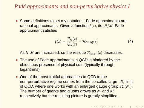
• Some definitions to set my notations: Padé approximants arerational approximants. Given a function f (z), its [N/M] Padéapproximant satisfies

f (z) =PM(z)QN(z)

+ R[N,M](z) (4)

As N,M are increased, so the residue R[N,M](z) decreases.

• The use of Padé approximants in QCD is hindered by theobiquitous presence of physical cuts (typically throughlogarithms).

• One of the most fruitful approaches to QCD in thenon-perturbative regime comes from the so-called large−Nc limitof QCD, where one works with an enlarged gauge group SU(Nc).The number of quarks and gluons grows as Nc and N2

crespectively but the resulting picture is greatly simplified.

Padé approximants and non-perturbative physics II

• Assuming confinement, the theory can be shown to lead to analmost idylic hadronic world of stable and non-interactingresonances.

• Besides its numerous phenomenological successes, the mostinteresting thing is that all correlators are meromorphic atleading order in 1/Nc.

• If one adopts the framework of large-Nc QCD, one can use thetheory of Padé approximants to meromorphic functions.

Padé approximants and the hadronic spectrum I

• One of the first attempts to derive the hadronic spectrum ofvector mesons was actually inspired by Padé approximants. Theeasiest way is to start with the two-point correlator

Πµν

V (q) = i∫

d4x eiq·x〈 0 |T{Vµ

ud(x) Vν

du(0) }| 0 〉

= (qµqν − q2gµν)ΠV(q2) (5)

whose singularities are poles (for stable particles) and cuts (dueto decaying resonances). In the large-Nc limit only the formersurvive.

• Next, one can try to build the [N/M] Padé approximant for ΠV(q2)as follows

ΠV(q2) = Π[N,M]V (q2) + R[N,M](q

2) , Π[N,M]V (q2) ≡ PM(q2)

QN(q2), (6)

The correlator is of Stieltjes type, and therefore the Padé polesare going to lie on the physical axis.

Padé approximants and the hadronic spectrum II

• By definition, the following equation is satisfied:

dn

d(q2)n

[

ΠV(q2)QN(q2) − PN(q2)

]∣

∣

∣

∣

q2=−µ2

= 0, n = 0, ..., 2N .

(7)

• Note that after the first N equations there is no contribution fromPN(q2). The analytical structure of ΠV(q2)QN(q2) contains onlysingle poles (the ones from ΠV(q2)). Cauchy’s theorem thereforeleads to

∫

∞

0

dt(t + µ2)n+1

ImΠV(t)QN(t) = 0, n = N + 1, ..., 2N , (8)

• The problem is to sort out the input for ImΠV(t) to be used in theprevious equation. In QCD at large enough energies (in theEuclidean) the leading term is a constant. This was originallytaken as the seed, with the hope that more information (bothperturbative and OPE) could be added later on to improve theresult.

Padé approximants and the hadronic spectrum III

• The solution for QN(t) can then be shown to lead to Legendrepolynomials P(0,0)

N ,

QN(q2) = 2F1

(

−N,−N; 1;− q2

µ2

)

= (q2 + µ2)N P(0,0)N

(

µ2 − q2

µ2 + q2

)

(9)which is actually a result due originally to Gauβ. Eq.(9) can nowbe plugged back in Eq.(7) to yield

[Weideman’05]

ΠNV(q2) ≃ 2

(q2 + µ2)N

N∑

k=0

(

kj

)2[

HN−k − Hk

P(0,0)N (χ)

]

(

− q2

µ2

)k

, χ =µ2 − q2

µ2 + q2,

(10)which is the Padé approximant to the logarithm, i.e., in thecontinuum limit N → ∞ we recover the logarithm we startedfrom.

Padé or not Padé? I

• The main motivation behind [Migdal’77] was to infer informationfrom the hadronic spectrum (discrete) starting from theconformal limit of the correlator. The following correlated limitwas taken instead,

q2 << µ2, N → ∞,Nµ

= ct. (11)

• Then

limq2→0

χ =

(

1 − 2q2

µ2

)

(12)

and

limN→∞

P(0,b)N

(

1 − ξ2

2N2

)

= J0(ξ) (13)

Padé or not Padé? II• The vector correlator takes the form

ΠNV(q2) = −4

3Nc

(4π)2

[

logq2

µ2− π

Y0 (qΛ )

J0 (qΛ )

]

, Λ =2Nµ. (14)

and the poles of the propagator (the masses of the physicalparticles in the large-Nc limit) are located at the zeroes of the J0

Bessel function.

• Obviously, the correlated limit does not retrieve the originalfunction and should not be called a Padé approximant. The truePadé approximant takes the form

ΠNV(q2) = −4

3Nc

(4π)2log

−q2

µ2− RN(q2)

QN(q2), (15)

where the residue is a Meijer G function that vanishes in thecontinuum limit, thus ensuring convergence. The correlatedlimits taken by Migdal freeze the residue, thereby spoiling theconvergence of the rational approximant. The non-vanishingresidue also explains why the resulting spectrum has distinctresonances after N → ∞.

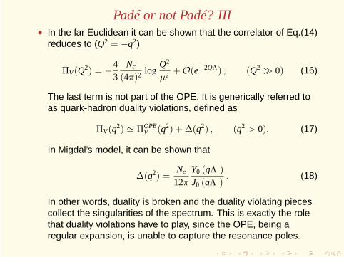
Padé or not Padé? III• In the far Euclidean it can be shown that the correlator of Eq.(14)

reduces to (Q2 = −q2)

ΠV(Q2) = −43

Nc

(4π)2log

Q2

µ2+ O(e−2QΛ) , (Q2 ≫ 0). (16)

The last term is not part of the OPE. It is generically referred toas quark-hadron duality violations, defined as

ΠV(q2) ≃ ΠOPEV (q2) + ∆(q2) , (q2 > 0). (17)

In Migdal’s model, it can be shown that

∆(q2) =Nc

12πY0 (qΛ )

J0 (qΛ ). (18)

In other words, duality is broken and the duality violating piecescollect the singularities of the spectrum. This is exactly the rolethat duality violations have to play, since the OPE, being aregular expansion, is unable to capture the resonance poles.

Connection with 5-dimensional models I• The AdS/CFT philosophy: given a string theory in AdS5 ×M5

with a 4-dimensional boundary, then the values of on-shell fields(in the supergravity limit) on the boundary are the externalsources of a CFT living on the boundary.

CFT

AdS5 ×M5

1

• Applications for non-conformal field theories (like QCD) rather adhoc. For instance, the simplest action in the gravity side:

S= −∫

d4x dz e−Φ(z)√g1

4g25

Tr

[

FµνFµν

]

, (19)

where gµν is the AdS metric

gµν dxµdxν =1z2

(ηµνdxµdxν + dz2) , ηµν = diag(−1, 1, 1, 1)

Connection with 5-dimensional models II

• Φ(z) is the dilaton field. In the hard wall model (HWM),

Φ(z) = φ, ǫ ≤ z≤ Λ ,

where z = ǫ and z = Λ are the four-dimensional boundarybranes.

• The problem therefore reduces to QFT in a box. It turns out thatthis action with these particular boundary conditions is dual tothe (non)-Padé construction before.

• I regard this as a mere curiosity: after all, Migdal’s approach isnot a Padé approximant; and the spectrum inferred by the HWMdoes not comply with expected properties of string theory (andphenomenology) such as Regge trajectories.

Padé approximants and electroweak observables I

• Computing the spectrum of large-Nc QCD is extremelycomplicated, and even so it is not clear its connection with theone in QCD.

• Unlike in the Minkowski axis, large-Nc in the Euclideanapproximates better QCD. We can use the drawbacks of lastsection to our advantage: since one cannot infer the QCDspectrum from the OPE, a reasonable job can be made with anarbitrary spectrum as long as it satisfies the OPE. For manyapplications (those involving Euclidean regimes) one does notneed the spectrum.

• Electroweak observables fall into this cathegory. In fullgenerality, they can all be expressed as integrals over Euclideanregimes of QCD correlators. For instance,

∆m2π

= m2π+ − m2

π0 = −3αEM

4πf 2π

∫

∞

0dQ2Q2ΠLR(Q2) (20)

Padé approximants and electroweak observables II• The MHA is a prescription to compute such observables using

truncated large-Nc ansätze for the correlators, while payingattention to fulfill what is known from QCD. For instance, we canchoose as ansatz:

ΠLR(q2) =f 2π

q2+

f 2V

−q2 + m2V

− f 2A

−q2 + m2A

(21)

and require the two following superconvergence relations(Weinberg sum rules):

∫

∞

0dt Im ΠLR(t) = 0

∫

∞

0dt t Im ΠLR(t) = 0 (22)

The correlator then looks like

ΠLR(q2) =m2

V m2A f 2

π

q2(−q2 + m2V)(−q2 + m2

A)(23)

Padé approximants and electroweak observables III• The free parameters mV, mA, fπ are fixed from phenomenology.

One can now compare the ansatz with experimental data:

Q MV2

2/

ALEPH

-Q Π Q2LR

( )2

2_ x

0 1 2 3 4 5 6 7

0.2

0.4

0.6

0.8

1

χQM

ENJL

BBG, HKPSB

C

F0

• The MHA is both an approximation to large-Nc QCD and aPadé-type approximant. Ideally, when N is infinitely large, thePadé-type to the correlator is actually the spectrum of large-Nc

QCD.

Padé approximants and electroweak observables IVShopping list:

• identify a suitable underlying correlator (both simple and orderparameter) to the observable under study.

• Compute its high energies with pQCD (in the same scheme asthe Wilson coefficients) and low energies with ChPT.

• Build a Padé-type interpolator, where the number of states(poles) is dictated by

N − P =1

2πi

∮

Σ′(z)Σ(z)

dz≃ −pOPE (24)

where Σ(z) is the propagator with no poles at the origin.

• The correlator so constructed can be matched to high and/or lowenergies. In practice, a balance between the two regimes tendsto be optimal.

Padé approximants and OPE/ChPT relations I

• One of the main advantages of the simplicity of the large-Nc limitis that, once the poles and residues are known, the full correlatoris known. In particular, there is a relation between OPE andChPT coefficients which can be used to test phenomenologicalanalyses.

• Consider in particular the ΠLR(q2) correlator, whose spectrumhas been reconstructed by very precise data on the decays ofthe tau lepton. At high energies, it can be parameterised by OPEcondensates, starting with ξ6 and ξ8 (ξ2 = 0 = ξ4):

limq2→(−∞)

ΠLR(q2) =∞∑

n=3

ξ2n

q2n(25)

whereas at low energies the ChPT Lagrangian yields

limq2→0

ΠLR(q2) =f 2π

q2− 8 L10 + 16 C87 q2 + O(q4) (26)

Padé approximants and OPE/ChPT relations II

• At present there is a puzzle: many groups have performedanalyses on the tau data, and while they find agreement on L10,the values for the OPE condensates are controversial. If wesucceed in connecting the two regimes, we can make, within ourapproximation, a consistency check.

• The ansatz for the correlator will be

ΠLR(q2) =f 2π

q2+

f 2V

−q2 + m2V

− f 2A

−q2 + m2A

(27)

If we want to leave poles and residues free we have to solve thefollowing system of equations:

f 2A − f 2

V = −f 2π

f 2Am2

A − f 2Vm2

V = 0

f 2Am4

A − f 2Vm4

V = ξ6

f 2Am6

A − f 2Vm6

V = ξ8 (28)

Padé approximants and OPE/ChPT relations III

• Its solution for the hadronic parameters in terms of fπ, ξ6 and ξ8

is highly non-linear. There are 4 sets of solutions and (notsurprisingly) in all of which the majority of parameters take oncomplex values. Indeed, ΠLR is not of Stieltjes type.

• Surprisingly (at least to me) the connection between low andhigh energy parameters is extremely simple:

L10 =18

[

f 2A

m2A

− f 2V

m2V

]

= −18ξ8

ξ26

f 4π

(29)

• The first thing to realize is that, since L10 = (−5.22 ± 0.06) · 10−3,ξ8 is predicted to be positive. There is a rigorous theorem byWitten which already fixes the sign of ξ6 to be positive.

• Even more importantly, Eq. (29) is satisfied at the quantitativelevel by the phenomenological analyses that already predictξ8 > 0.

Padé approximants and OPE/ChPT relations IV

ξ6 ξ8 ξ8 = −8 L10 f−4π ξ2

6

Friot et al. +7.90 ± 1.63 +11.69 ± 2.55 +9.0 ± 3.7

Ioffe et al. +6.8 ± 2.1 +7 ± 4 +6.7 ± 4.1

Zyablyuk +7.2 ± 1.2 +7.8 ± 2.5 +7.5 ± 2.5

Narison +8.7 ± 2.3 +15.6 ± 4.0 +10.9 ± 5.8

ALEPH +8.2 ± 0.4 +11.0 ± 0.4 +9.71 ± 0.96

OPAL +6.0 ± 0.6 +7.6 ± 1.5 +5.2 ± 1.0

Cirigliano et al. on ALEPH +4.45 ± 0.70 −6.16 ± 3.11 +2.86 ± 0.90

Cirigliano et al. on OPAL +5.43 ± 0.76 −1.35 ± 3.47 +4.3 ± 1.2

Bijnens et al. on ALEPH +3.4+2.4−2.0 −14.4+10.4

−8.0 +1.7 ± 2.4

Bijnens et al. on OPAL +4.0 ± 2.0 −10.4+8.0−6.4 +2.3 ± 2.3

Latorre et al. +4.0 ± 2.0 −12+7−11 +2.3 ± 2.3

Almasy et al. 3.2+1.6−0.4 −17.0+2.5

−9.5 +1.5 ± 1.5

Padé approximants and OPE/ChPT relations V

0 2 4 6 8 10 12

-20

-10

0

10

20

Ξ6

Ξ8

Summary I

• Padé approximants are not the right tool to determine thespectrum of QCD. Such a Padé can only be the approximant tosomething that is already known from the beginning. Insertingas input the leading order in the Euclidean regime is flawed formany reasons: first and foremost, different spectrums may leadto the same (asymptotic) OPE. In other words, the analyticalcontinuation from the Euclidean to the physical axis dependscrucially on the singularities of the correlator, which is actuallythe result one would like to find. The naive analyticalcontinuation of Migdal is clearly inconsistent with the (assumed)large-Nc limit. Actually, even inserting an input into the correlatoris an exercise in circular logic.

Summary II

• In order to study electroweak observables, Padé-typeapproximants to meromorphic functions, realized in the form ofthe MHA, have provided valuable aid as interpolators betweenthe high and low energy of the underlying correlators. Theresults seem to be numerically sound but since the correlatorsare order parameters, only Pommerenke’s theorem can beinvoked.

• There is a common misconception: large-Nc and Padé poles andresidues can be identified. This is only true when there is infiniteinformation (and then we do not need to use Padé’s at all). For afinite amount of information, one needs to leave at least theresidues to be fixed.

Summary III

• For some applications (when interpolation is not the main goal) itis preferable to use conventional Padés. For instance, whenlooking for analytical relations between low and high energyparameters. Given a fixed number of poles, a conventional Padérequires more constraints than a Padé-type. Rule of thumb: ifinterpolator is needed and there is scarcity of constraints,Padé-types are the best choice. If, on the other hand, one isinterested in high energy prediction, we might not want themasses to be fixed. Conventional Padé’s are then the rightchoice.

Documents

Pad approximants and the prediction of non-perturbative