Embed Size (px)
Citation preview

Packet Scheduling under Imperfect Channel Conditions in Long Term Evolution (LTE)
A Thesis
submitted to
University of Technology, Sydney
by
Yongxin Wang
In accordance with
the requirements for the Degree of
Master of Engineering
Faculty of Engineering and Information Technology
University of Technology, Sydney
New South Wales, Australia
October 2013

- ii -
CERTIFICATE OF AUTHORSHIP/ORIGINALITY
I certify that the work in this thesis has not previously been submitted for a degree nor
has it been submitted as part of requirements for a degree except as fully acknowledged
with the text.
I also certify that the thesis has been written by me. Any help that I have received in my
research work and the preparation of the thesis itself has been acknowledged. In
addition, I certify that all information sources and literature used are indicated in the
thesis.
Signature of Candidate
___________________________________

- iii -
ACKNOWLEDGMENT
I wish to express my utmost gratitude to my supervisor, Assoc. Prof. Dr Kumbesan
Sandrasegaran for his sound advice, logical way of thinking, and even more important
to me, for his understanding, patience and encouragement. I would never be able to
cross the hurdle and complete my work on target without his support.
I would like to acknowledge members of my advisory committee: Dr Xiaoying Kong
(co-supervisor) and Assoc. Prof. Dr Xinning Zhu for their valuable suggestions and
encouragement.
I would like to extend my appreciation to my close friends and all CRIN members for
their friendly support and caring.
My deepest gratitude goes to my family and my husband Jingjing Fei for their
emotional and moral support and for helping me get through the difficult times. Without
their encouragement, it would have been impossible for me to complete this research
work.
Finally, I am dedicating this to my baby, whose heart melting smile and peaceful
sleeping face always give me courage, motivation and love.
- iv -
ABSTRACT
The growing demand for high speed wireless data services, such as Voice Over Internet
Protocol (VoIP), web browsing, video streaming and gaming, with constraints on
system capacity and delay requirements, poses new challenges in future mobile cellular
systems. Orthogonal Frequency Division Multiple Access (OFDMA) is the preferred
access technology for downlink Long Term Evolution (LTE) standardisation as a
solution to the challenges. As a network based on an all-IP packet switched architecture,
LTE employs packet scheduling to satisfy Quality of Service (QoS) requirements.
Therefore, efficient design of packet scheduling becomes a fundamental issue. The aim
of this thesis is to propose a novel packet scheduling algorithm to improve system
performance for practical downlink LTE system.
This thesis first focuses on time domain packet scheduling algorithms. A number of
time domain packet scheduling algorithms are studied and some well-known time
domain packet scheduling algorithms are compared in downlink LTE. A packet
scheduling algorithm is identified that it is able to provide a better trade-off between
maximizing the system performance and guaranteeing the fairness.
Thereafter, some frequency domain packet schemes are introduced and examples of
QoS aware packet scheduling algorithms employing these schemes are presented. To
balance the scheduling performance and computational complexity and be tolerant to
the time-varying wireless channel, a novel scheduling scheme and a packet scheduling
algorithm are proposed. Simulation results show this proposed algorithm achieves an
overall reasonable system performance.
Packet scheduling is further studied in a practical channel condition environment which
assumes imperfect Channel Quality Information (CQI). To alleviate the performance
degradation due to simultaneous multiple imperfect channel conditions, a packet
scheduling algorithm based on channel prediction and the proposed scheduling scheme
is developed in downlink LTE system for GBR services. It was shown in simulation
results that the Kalman filter based channel predictor can effectively recover the correct
- v -
CQI from erroneous channel quality feedback, therefore, the system performance is
significantly improved.
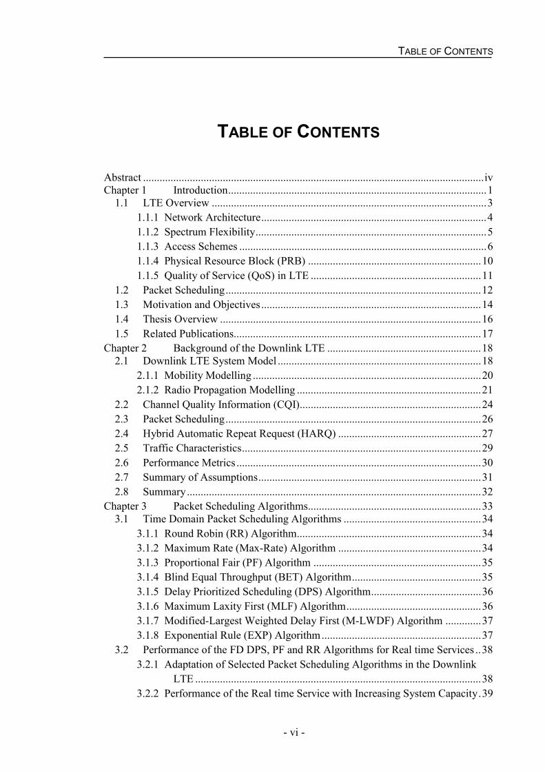
TABLE OF CONTENTS
- vi -
TABLE OF CONTENTS
Abstract ............................................................................................................................iv Chapter 1 Introduction..............................................................................................1
1.1 LTE Overview ....................................................................................................3
1.1.1 Network Architecture..................................................................................4
1.1.2 Spectrum Flexibility....................................................................................5
1.1.3 Access Schemes ..........................................................................................6
1.1.4 Physical Resource Block (PRB) ...............................................................10
1.1.5 Quality of Service (QoS) in LTE ..............................................................11
1.2 Packet Scheduling.............................................................................................12
1.3 Motivation and Objectives................................................................................14
1.4 Thesis Overview ...............................................................................................16
1.5 Related Publications..........................................................................................17
Chapter 2 Background of the Downlink LTE ........................................................18 2.1 Downlink LTE System Model ..........................................................................18
2.1.1 Mobility Modelling ...................................................................................20
2.1.2 Radio Propagation Modelling ...................................................................21
2.2 Channel Quality Information (CQI)..................................................................24
2.3 Packet Scheduling.............................................................................................26
2.4 Hybrid Automatic Repeat Request (HARQ) ....................................................27
2.5 Traffic Characteristics.......................................................................................29
2.6 Performance Metrics .........................................................................................30
2.7 Summary of Assumptions.................................................................................31
2.8 Summary...........................................................................................................32
Chapter 3 Packet Scheduling Algorithms...............................................................33 3.1 Time Domain Packet Scheduling Algorithms ..................................................34
3.1.1 Round Robin (RR) Algorithm...................................................................34
3.1.2 Maximum Rate (Max-Rate) Algorithm ....................................................34
3.1.3 Proportional Fair (PF) Algorithm .............................................................35
3.1.4 Blind Equal Throughput (BET) Algorithm...............................................35
3.1.5 Delay Prioritized Scheduling (DPS) Algorithm........................................36
3.1.6 Maximum Laxity First (MLF) Algorithm.................................................36
3.1.7 Modified-Largest Weighted Delay First (M-LWDF) Algorithm .............37
3.1.8 Exponential Rule (EXP) Algorithm..........................................................37
3.2 Performance of the FD DPS, PF and RR Algorithms for Real time Services ..38
3.2.1 Adaptation of Selected Packet Scheduling Algorithms in the Downlink LTE ........................................................................................................38
3.2.2 Performance of the Real time Service with Increasing System Capacity.39
TABLE OF CONTENTS
- vii -
3.3 Summary...........................................................................................................46
Chapter 4 QoS Aware Scheduling Schemes and Algorithms ................................47 4.1 Resource Allocation and Assignment (RAA) Scheme .....................................48
4.1.1 Load-oriented Scheduling (LOS) Algorithm ............................................49
4.1.2 Delay First Scheduling (DFS) Algorithm .................................................50
4.1.3 Multi-QoS Adaptive Scheduling (MQAS) Algorithm..............................51
4.2 Joint Time and Frequency Domain Scheduling (JTFDS) Scheme ...................53
4.3 Matrix-Based Scheduling (MBS) Scheme........................................................55
4.4 QoS-Oriented Grouping Scheduling (QOGS) Scheme.....................................57
4.4.1 Parity Grouping Scheduling (PGS) Algorithm .........................................59
4.4.2 Performance of the PGS algorithm for real time services.........................61
4.5 Summary...........................................................................................................71
Chapter 5 Packet Scheduling with Imperfect CQI .................................................73 5.1 Packet Scheduling Algorithms under Practical Channel Condition .................74
5.1.1 HARQ Aware Scheduling (HAS) Algorithm ...........................................74
5.1.2 Robust and QoS-Driven Scheduling (RQ-DS) Algorithm........................75
5.1.3 HARQ Aware TD-FD Scheduling (HATFS) Algorithm..........................76
5.1.4 Advanced Proportionally Fair Scheduling (APFS) Algorithm .................77
5.2 Channel Prediction............................................................................................78
5.2.1 Least Squares Estimation ..........................................................................78
5.2.2 Kalman Filter ............................................................................................79
5.3 Channel Predictive Grouping Scheduling (CPGS) Algorithm .........................84
5.3.1 Kalman Filter for Channel Prediction .......................................................85
5.3.2 Initialization of the Kalman Filter.............................................................87
5.3.3 Channel Predictive Grouping Scheduling (CPGS) Algorithm Based on the Kalman Filter .........................................................................................90
5.4 Results and Discussions....................................................................................91
5.4.1 Performance of Kalman filter....................................................................93
5.4.2 Performance of the CPGS Algorithm for Real Time Services .................95
5.5 Summary.........................................................................................................102
Chapter 6 Conclusions and Future Research Directions ......................................104 6.1 Summary of Thesis Contributions ..................................................................104
6.1.1 Providing an overall good performance to support QoS.........................104
6.1.2 Providing Robust Performance under Imperfect Channel Conditions....105
6.2 Future Research Directions.............................................................................105
References .....................................................................................................................107
LIST OF FIGURES
- viii -
LIST OF FIGURES
Figure 1.1: Growth rates of population and mobile-cellular subscriptions [2] .................1Figure 1.2: Evolution of the mobile cellular systems [10] ................................................3Figure 1.3: 3G evolution [13] ...........................................................................................4Figure 1.4: Evolution of 3GPP standards [14] ..................................................................4Figure 1.5: UTRAN and eUTRAN Network Architecture [16] .......................................5Figure 1.6: Scalable bandwidth in LTE [19] .....................................................................5Figure 1.7: Migration of spectrum allocation from GSM to LTE [1] ...............................6Figure 1.8: Spectrum allocations in FDD and TDD modes [20] ......................................6Figure 1.9: QPSK data transmission in OFDMA and SC-FDMA [21] ............................7Figure 1.10: Adjacent sub-carrier with OFDM [16] .........................................................8Figure 1.11: OFDM signal represented in frequency and time [21] .................................8Figure 1.12: Frequency selective fading - single carrier vs. OFDM [16] .........................9Figure 1.13: OFDM and OFDMA sub-carrier allocation [21] ..........................................9Figure 1.14: PRB representation in time and frequency domains using a normal CP [23]
.........................................................................................................................................10Figure 1.15: Time-frequency selective fading in channel dependent scheduling [16] ...13Figure 1.16: General packet scheduling model for downlink wireless system [30] .......14Figure 2.1: Multi-cell simulation environment ...............................................................19Figure 2.2: Illustration of a wrapped-around process .....................................................20Figure 2.3: Frequency flat Rayleigh fading structure [40] ..............................................22Figure 2.4: SINR-to-CQI mapping for 10% BLER threshold ........................................24Figure 2.5: A TB structure diagram [23] ........................................................................27Figure 2.6: A complete cycle of the SAW protocol [57] ................................................29Figure 2.7: A sample of CBR traffic for 1 Mbps data rate for 1000 ms .........................29Figure 3.1: System throughput comparison ....................................................................41Figure 3.2: PLR comparison ...........................................................................................42Figure 3.3: Fairness comparison .....................................................................................44Figure 3.4: Average system delay comparison ...............................................................45Figure 4.1: Flow chart of the RAA scheme in each TTI .................................................49Figure 4.2: The structure of JTFDS scheme ...................................................................53Figure 4.3: MBS Channel Matrix ...................................................................................56Figure 4.4: An illustration of the QOGS scheme ............................................................58Figure 4.5: Flow chart of the PGS algorithm in each TTI ..............................................60Figure 4.6: System throughput comparison -3km/h ........................................................64Figure 4.7 System throughput comparison -30km/h .......................................................65Figure 4.8: PLR comparison -3km/h ...............................................................................66Figure 4.9: PLR comparison -30km/h .............................................................................67Figure 4.10: Fairness comparison -3km/h .......................................................................68Figure 4.11: Fairness comparison -30km/h .....................................................................68Figure 4.12: Average system delay comparison -3km/h .................................................70Figure 4.13: Average system delay comparison -30km/h ...............................................70Figure 5.1: State-space model of the Kalman filter ........................................................87Figure 5.2: Flow chart of the CPGS algorithm ...............................................................90
LIST OF FIGURES
- ix -
Figure 5.3 Comparison of the estimated SINR and the realistic SINR of User 2 ...........93Figure 5.4: Comparison of the estimated SINR and the realistic SINR of User 5 ..........94Figure 5.5: Estimate error probabilities ..........................................................................95Figure 5.6: System throughput comparison -3km/h ........................................................96Figure 5.7: System throughput comparison -30km/h ......................................................96Figure 5.8: PLR comparison -3km/h ...............................................................................98Figure 5.9: PLR comparison -30km/h .............................................................................98Figure 5.10: Fairness comparison -3km/h .......................................................................99Figure 5.11: Fairness comparison -30km/h ...................................................................100Figure 5.12: Average system delay comparison -3km/h ...............................................101Figure 5.13: Average system delay comparison -30km/h .............................................102
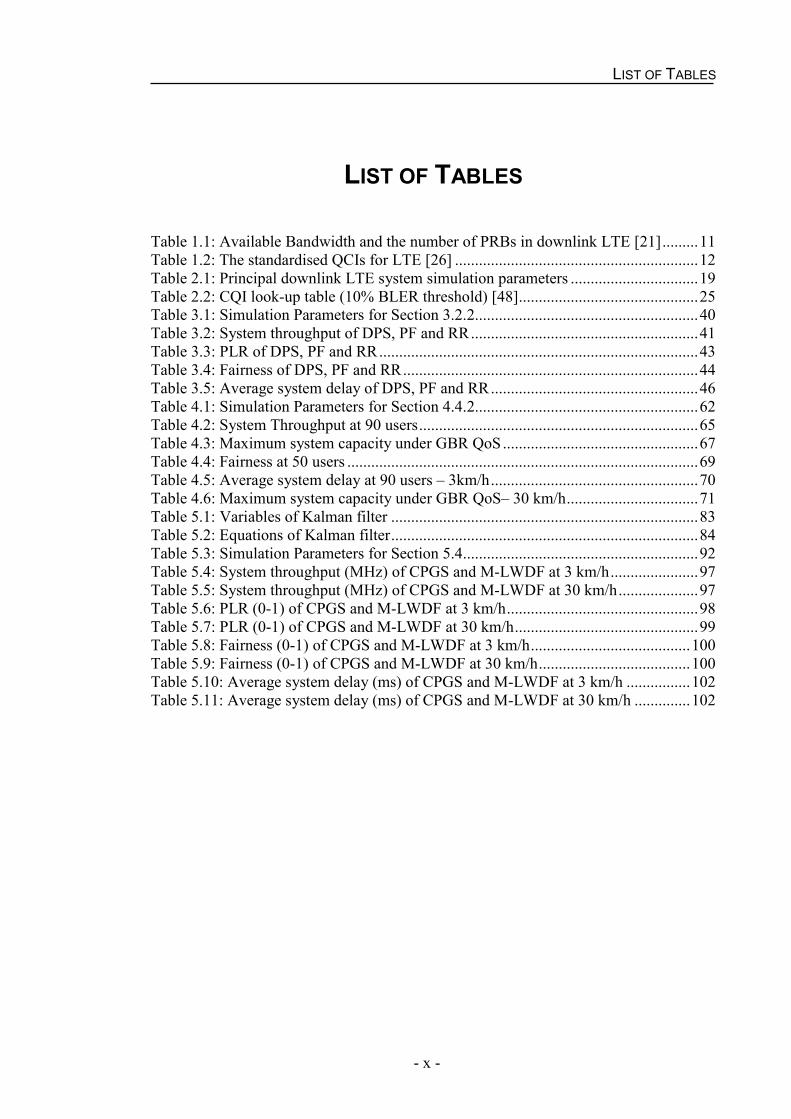
LIST OF TABLES
- x -
LIST OF TABLES
Table 1.1: Available Bandwidth and the number of PRBs in downlink LTE [21] .........11Table 1.2: The standardised QCIs for LTE [26] .............................................................12Table 2.1: Principal downlink LTE system simulation parameters ................................19Table 2.2: CQI look-up table (10% BLER threshold) [48] .............................................25Table 3.1: Simulation Parameters for Section 3.2.2 ........................................................40Table 3.2: System throughput of DPS, PF and RR .........................................................41Table 3.3: PLR of DPS, PF and RR ................................................................................43Table 3.4: Fairness of DPS, PF and RR ..........................................................................44Table 3.5: Average system delay of DPS, PF and RR ....................................................46Table 4.1: Simulation Parameters for Section 4.4.2 ........................................................62Table 4.2: System Throughput at 90 users ......................................................................65Table 4.3: Maximum system capacity under GBR QoS .................................................67Table 4.4: Fairness at 50 users ........................................................................................69Table 4.5: Average system delay at 90 users – 3km/h ....................................................70Table 4.6: Maximum system capacity under GBR QoS– 30 km/h .................................71Table 5.1: Variables of Kalman filter .............................................................................83Table 5.2: Equations of Kalman filter .............................................................................84Table 5.3: Simulation Parameters for Section 5.4 ...........................................................92Table 5.4: System throughput (MHz) of CPGS and M-LWDF at 3 km/h ......................97Table 5.5: System throughput (MHz) of CPGS and M-LWDF at 30 km/h ....................97Table 5.6: PLR (0-1) of CPGS and M-LWDF at 3 km/h ................................................98Table 5.7: PLR (0-1) of CPGS and M-LWDF at 30 km/h ..............................................99Table 5.8: Fairness (0-1) of CPGS and M-LWDF at 3 km/h ........................................100Table 5.9: Fairness (0-1) of CPGS and M-LWDF at 30 km/h ......................................100Table 5.10: Average system delay (ms) of CPGS and M-LWDF at 3 km/h ................102Table 5.11: Average system delay (ms) of CPGS and M-LWDF at 30 km/h ..............102
LIST OF ACRONYMS
- xi -
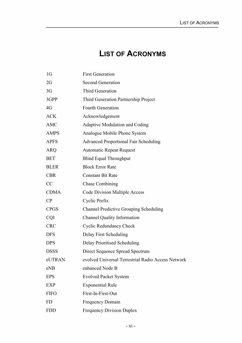
LIST OF ACRONYMS
1G First Generation
2G Second Generation
3G Third Generation
3GPP Third Generation Partnership Project
4G Fourth Generation
ACK Acknowledgement
AMC Adaptive Modulation and Coding
AMPS Analogue Mobile Phone System
APFS Advanced Proportional Fair Scheduling
ARQ Automatic Repeat Request
BET Blind Equal Throughput
BLER Block Error Rate
CBR Constant Bit Rate
CC Chase Combining
CDMA Code Division Multiple Access
CP Cyclic Prefix
CPGS Channel Predictive Grouping Scheduling
CQI Channel Quality Information
CRC Cyclic Redundancy Check
DFS Delay First Scheduling
DPS Delay Prioritised Scheduling
DSSS Direct Sequence Spread Spectrum
eUTRAN evolved Universal Terrestrial Radio Access Network
eNB enhanced Node B
EPS Evolved Packet System
EXP Exponential Rule
FIFO First-In-First-Out
FD Frequency Domain
FDD Frequency Division Duplex
LIST OF ACRONYMS
- xii -
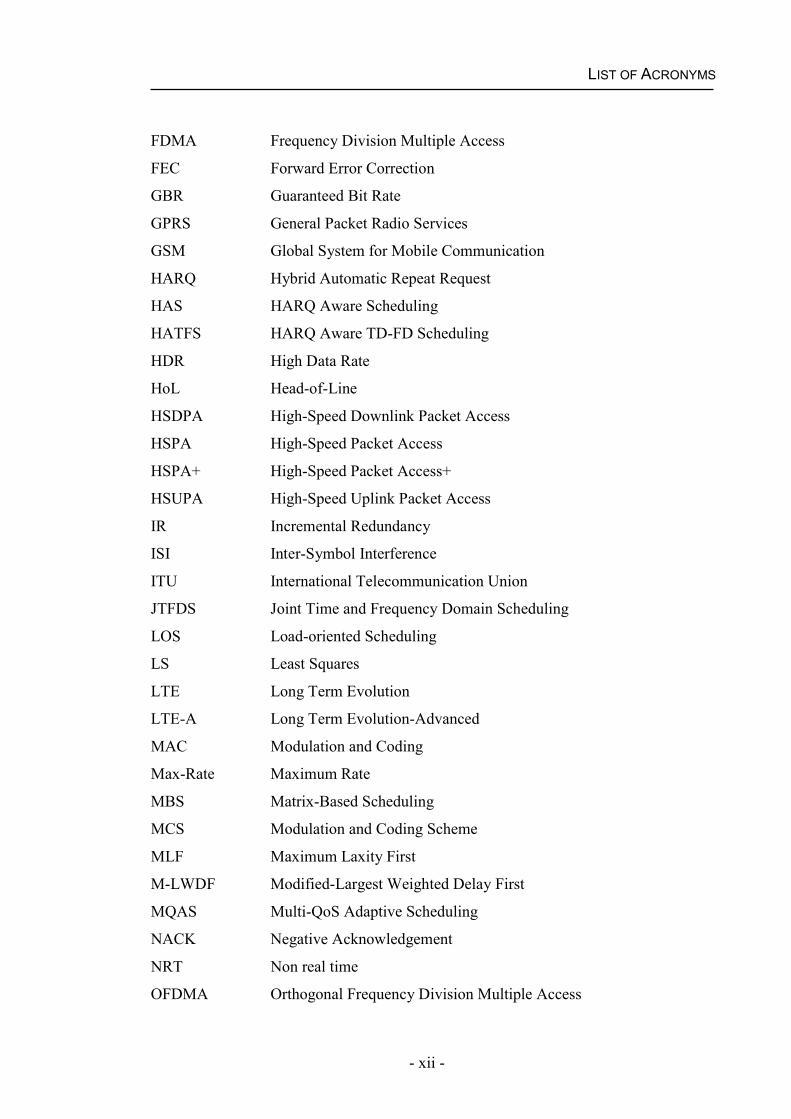
FDMA Frequency Division Multiple Access
FEC Forward Error Correction
GBR Guaranteed Bit Rate
GPRS General Packet Radio Services
GSM Global System for Mobile Communication
HARQ Hybrid Automatic Repeat Request
HAS HARQ Aware Scheduling
HATFS HARQ Aware TD-FD Scheduling
HDR High Data Rate
HoL Head-of-Line
HSDPA High-Speed Downlink Packet Access
HSPA High-Speed Packet Access
HSPA+ High-Speed Packet Access+
HSUPA High-Speed Uplink Packet Access
IR Incremental Redundancy
ISI Inter-Symbol Interference
ITU International Telecommunication Union
JTFDS Joint Time and Frequency Domain Scheduling
LOS Load-oriented Scheduling
LS Least Squares
LTE Long Term Evolution
LTE-A Long Term Evolution-Advanced
MAC Modulation and Coding
Max-Rate Maximum Rate
MBS Matrix-Based Scheduling
MCS Modulation and Coding Scheme
MLF Maximum Laxity First
M-LWDF Modified-Largest Weighted Delay First
MQAS Multi-QoS Adaptive Scheduling
NACK Negative Acknowledgement
NRT Non real time
OFDMA Orthogonal Frequency Division Multiple Access
LIST OF ACRONYMS
- xiii -
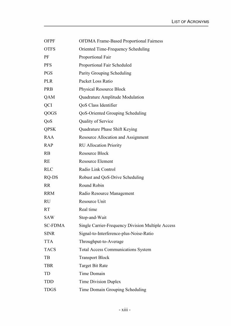
OFPF OFDMA Frame-Based Proportional Fairness
OTFS Oriented Time-Frequency Scheduling
PF Proportional Fair
PFS Proportional Fair Scheduled
PGS Parity Grouping Scheduling
PLR Packet Loss Ratio
PRB Physical Resource Block
QAM Quadrature Amplitude Modulation
QCI QoS Class Identifier
QOGS QoS-Oriented Grouping Scheduling
QoS Quality of Service
QPSK Quadrature Phase Shift Keying
RAA Resource Allocation and Assignment
RAP RU Allocation Priority
RB Resource Block
RE Resource Element
RLC Radio Link Control
RQ-DS Robust and QoS-Drive Scheduling
RR Round Robin
RRM Radio Resource Management
RU Resource Unit
RT Real time
SAW Stop-and-Wait
SC-FDMA Single Carrier-Frequency Division Multiple Access
SINR Signal-to-Interference-plus-Noise-Ratio
TTA Throughput-to-Average
TACS Total Access Communications System
TB Transport Block
TBR Target Bit Rate
TD Time Domain
TDD Time Division Duplex
TDGS Time Domain Grouping Scheduling
LIST OF ACRONYMS
- xiv -
TSN Transmission Sequence Number
TTI Transmission Time Interval
UE User Equipment
UMTS Universal Mobile Telecommunications System
UTRAN Universal Terrestrial Radio Access Network
WCDMA Wideband Code Division Multiple Access
LIST OF SYMBOLS
- xv -
LIST OF SYMBOLS
Constant parameter
Constant parameter
A small positive constant
t Additive noise
System noise
Learning rate
Proportion of the total RUs allocated to real time users at TTI t
Shadow fading standard deviation 2 Noise
,2 Covariance of Xe,r(t),2 Covariance of Xe,v(t),2 Covariance of Xe,b(t)
Variance (mean power)
i Service-dependent PLR threshold of user i
i(t) Approximated uncorrelated filtered white Gaussian noise with
zero mean of process i at time t
i(t) Priority of user i at scheduling interval t
n Uncorrelated filtered white Gaussian noise with zero mean of the
nth sinusoid
RTi(t) Priority for non real time users
i(t) Shadow fading autocorrelation function,
i,j SINR of user i on PRB j
i,j(t) Instantaneous SINR of user i on PRB j at time t
i,n Doppler phase of process i of the nth sinusoid
(t) Frequency flat Rayleigh fading at time t
i(t) Shadow fading gain of user i at time t
a System gain
ai QoS requirement of user i
a(hm) Mobile antenna correction factor
LIST OF SYMBOLS
- xvi -
aW_avg Average of QoS requirement and delay of the HoL packet across
all users ( ) State transition matrix
b A coefficient
bi Gradient of i,j
B(t) Input transition matrix
Bi(t) Total size of all packets (in bits) in the buffer(at base station) of
user i at scheduling interval t
ci,n Doppler coefficient (which represents a real weighting factor) of
process i of the nth sinusoid
d0 Shadow fading correlation distance
di(t) Time to live of the HoL packet of user i at TTI t
diri(t) Direction of user i at time t
|disi(t)| Magnitude of distance of user i from eNB at time t
DPl,i(t) Delay of the lth packet of user i at time t
Dretxi(t) Average retransmission delay of user i at scheduling interval t
et Estimation error
E[r] Expected mean data rate r
Ei,j(t) Element (in channel matrix) of user i on RU j at scheduling
interval t
Efficiencyi,j(t) Efficiency (in bits/RE) of PRB j of user i at time t
Exei(t) Execution time of user i at TTI t
fi,n Discrete Doppler frequency of process i of the nth sinusoid
fmax Maximum Doppler frequency
G(t) Gaussian random variable of user i at time t
hb Height of the eNB
Hi(t) Average channel gain of RUs for user i at TTI t
H(t) Observation matrix
I Identity matrix
Ii(t+1) Indicator function of the event that packets of user i are selected
for transmission at scheduling interval t+1
ICI Inter-cell interference
LIST OF SYMBOLS
- xvii -
k A variable of the summation to compute across all users
K(t) Kalman gain
laxi(t) Laxity time of user i at TTI t
loci(t) Location of user i at time t
mpathi,j(t) Multi-path fading gain of user i on PRB j at time t
ni(t) Number of RUs that is allocated to user i at scheduling interval t
nNRT(t) Number of RUs allocated to non real time users at scheduling
interval t
nRT(t) Number of RUs allocated to real time users at scheduling interval
t
N Total number of users
No Thermal noise
Ni Number of sinusoids of process i
Pt-1 Estimated error
pdiscardi(t) Total size of discarded packets (in bits) of user i at time t
pli(t) Path loss of user i at time t
prxi(t) Total size of correctly received packets (in bits) of user i at time t
psizei(t) Total size of all packets that have arrived to the eNB buffer of
user i at time t
Ptotal Total eNB transmit power( ) Update covariance matrix
PLRi(t) PLR of user i at scheduling interval t
PRBmax Maximum available number of PRBs
Q(t) State noise covariance matrix
Qi(t) Buffer length of user i at TTI t
ri(t) Instantaneous data rate(across the whole bandwidth) of user i at
scheduling interval t
ri,j(t) Instantaneous data rate of user i on RU j at scheduling interval t
rai(t) Average data rate over a number of scheduling intervals of user i
at scheduling interval t
ravgi(t) Average data rate over a number of scheduling intervals of user i
at scheduling interval t
LIST OF SYMBOLS
- xviii -
rtoti(t) Total number of bits supportable on the PRBs allocated to user i
at TTI t
R(t) Additive observation noise
Ri(t) Average throughput of user i at scheduling interval t
Rofpfi(t) Modified average throughput of user i at TTI t
R_reqi(t) Average throughput required by user i at scheduling interval t
R_schi(t) Estimated average throughput of user i at TTI t,( | 1) Covariance matrix at time conditioned on the estimate ( | 1)PRBrem Total number of remaining PRBs of all users
PRBHARQ Total number of PRBs required by all HARQ users
REdata Total number of REs specified for downlink data transmission
RUHARQ Total number of RUs required by all HARQ users
RUrem Remaining RUs
RUtotal Total available RUs at TTI t
T Total simulation time
tc A time constant
Ti Service-dependent buffer delay threshold of user i
Twaiti(t) Waiting time of user i from the last scheduled interval until now
TOAl,i Time of arrival of the lth packet of user i in the eNB buffer
u(t) Input vector
vi Change rate of SINR of user i
vi(t) Speed of user i at time t
Wi(t) Delay of the HOL packet of user i at time t
WRT(t) Allocation weight given to the real time users at TTI t
xt Current state
Estimation of
X(t|t-1) Estimated state at time t based on the estimate at time t-1
(t) Estimated state at time t
Xe,b(t) Measurement error of bi
Xe,r(t) Measurement error of i,j
Xe,v(t) Measurement error of vi
LIST OF SYMBOLS
- xix -
yt Measurement of
Zi(t) Sequence of observation values
- 1 -
Chapter 1
INTRODUCTION
The mobile and personal communication systems have developed rapidly since 1970s
[1]. The introduction of cellular phones has a major influence on human life as it offers
convenient and real time communication to a large number of mobile users within a
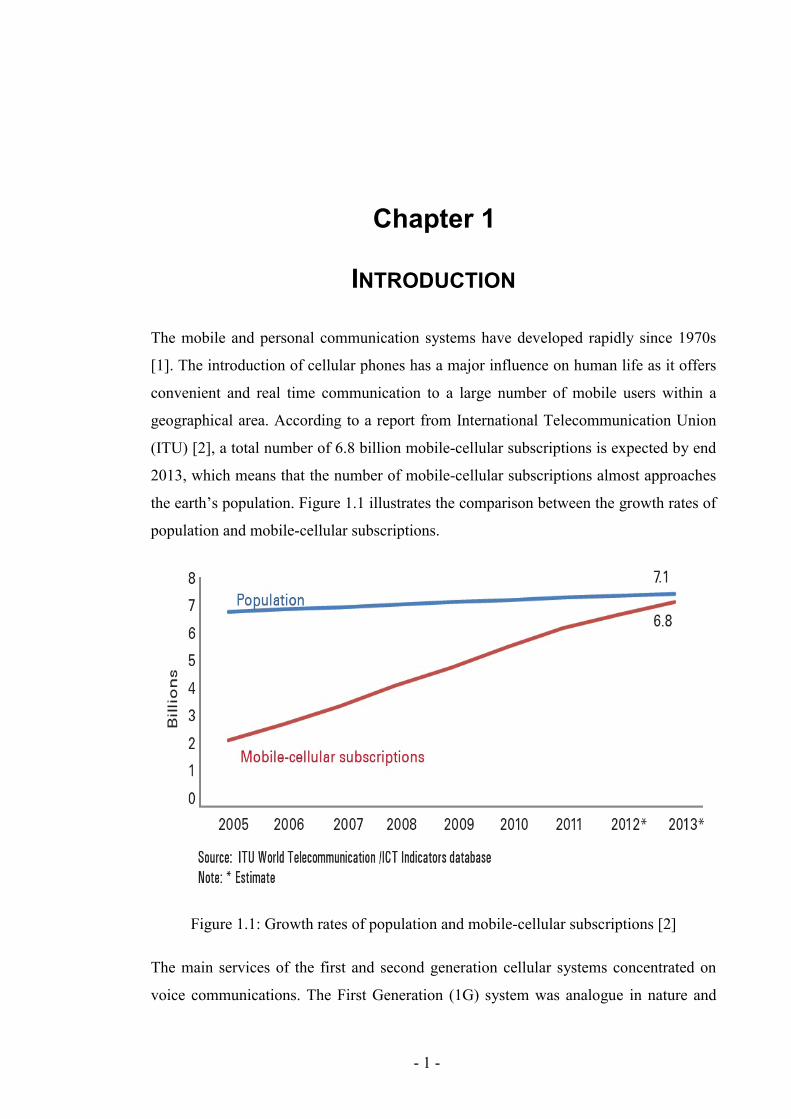
geographical area. According to a report from International Telecommunication Union
(ITU) [2], a total number of 6.8 billion mobile-cellular subscriptions is expected by end
2013, which means that the number of mobile-cellular subscriptions almost approaches
the earth’s population. Figure 1.1 illustrates the comparison between the growth rates of
population and mobile-cellular subscriptions.
Figure 1.1: Growth rates of population and mobile-cellular subscriptions [2]
The main services of the first and second generation cellular systems concentrated on
voice communications. The First Generation (1G) system was analogue in nature and
CHAPTER 1
- 2 -
used Frequency Division Multiple Access (FDMA) scheme [1]. Advanced Mobile
Phone System (AMPS) and Total Access Communications System (TACS) developed
in late 1970s and early 1980s, were widely deployed in North America and UK,
respectively. As the FDMA scheme required significant frequency resources (spectrum),
the first generation systems were replaced by the Second Generation (2G) systems with
increasing number of mobile users.
The 2G mobile cellular systems introduced in the early 1990s were mostly based on
circuit-switched technology. Most 2G systems such as Global System for Mobile
Communications (GSM) and Code Division Multiple Access (CDMA) were developed
to support voice and low speed data services [3]. As the low data rate cannot satisfy the
increasing demands of the Internet and higher speed multimedia services, General
Packet Radio Services (GPRS) which was known as 2.5G using packet-switched
technology emerged [4].
In the mean time, the research and development work of the Third Generation (3G)
cellular systems had been conducted and a pre-release based on Wideband CDMA
(WCDMA) technology was available in May 2001 [5]. In December 2001, a
commercial Universal Mobile Telecommunications System (UMTS) network, based on
Direct Sequence Spread Spectrum (DSSS) [6] was deployed in Europe to provide a
great spectral efficiency. UMTS was developed to be backward compatible with GSM.
The requirements for higher data rate services and the global success of the 3G wireless
systems led to the development of an enhanced 3G system in the High-Speed Packet
Access (HSPA) family which was called High-Speed Downlink Packet Access
(HSDPA). The deployment of Hybrid Automatic Repeat Request (HARQ), packet
scheduling and Adaptive Modulation and Coding (AMC) technologies are some of
HSDPA key features. Further improvements were made in the High-Speed Uplink
Packet Access (HSUPA) and High-Speed Packet Access + (HSPA+) systems.
The latest commercial mobile cellular system, Long Term Evolution (LTE), is referred
to as 3.9 G. The research phase began in late 2004 and first commercial network was
launched on 14 December 2009 [7]. The key project objectives were set in a series of
areas: flexible channel bandwidths, spectral efficiency, peak data throughput, latency

CHAPTER 1
- 3 -
and overall system cost [8]. An enhancement of the LTE standard was proposed by the
3rd Generation Partnership Project (3GPP) in September 2009 and is known as Long
Term Evolution-Advanced (LTE-A). It is a Fourth Generation (4G) system and the first
implementation of LTE-A was carried out in October 2012 by Russian network operator
Yota [9]. Figure 1.2 presents the evolution from 2G towards 4G cellular systems.
Figure 1.2: Evolution of the mobile cellular systems [10]
1.1 LTE Overview
As a long-term development of the 3G services, the first release of 3GPP LTE
specifications (i.e. Release 8) was completed in March 2009 [11]. According to the
specifications, the LTE is expected to provide better quality of wireless communication
in terms of high performance and capacity, simplicity and wide range of terminals. For
this purpose, a series of improvements in higher speeds, reduced latency, increased
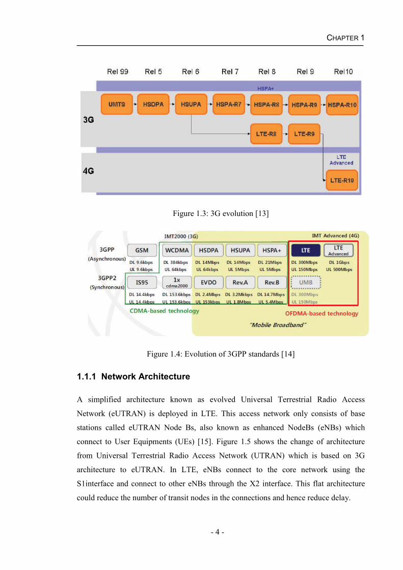
capacity and coverage is required [12]. Figure 1.3 presents the details of 3G evolutions
and Figure1.4 presents the evolution of 3GPP family standards. It can be seen in Figure
1.4 that the data rate has been significantly improved in each evolution step.
CHAPTER 1
- 4 -
Figure 1.3: 3G evolution [13]
Figure 1.4: Evolution of 3GPP standards [14]
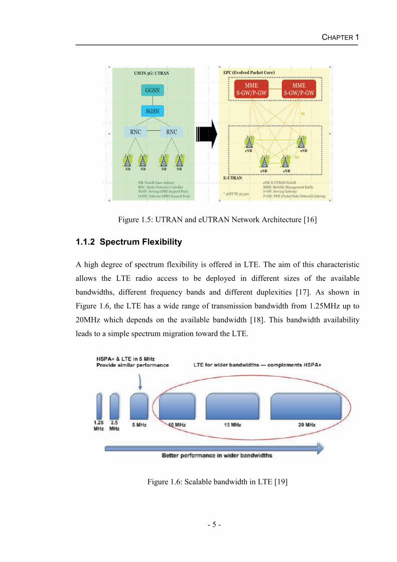
1.1.1 Network Architecture
A simplified architecture known as evolved Universal Terrestrial Radio Access
Network (eUTRAN) is deployed in LTE. This access network only consists of base
stations called eUTRAN Node Bs, also known as enhanced NodeBs (eNBs) which
connect to User Equipments (UEs) [15]. Figure 1.5 shows the change of architecture
from Universal Terrestrial Radio Access Network (UTRAN) which is based on 3G
architecture to eUTRAN. In LTE, eNBs connect to the core network using the
S1interface and connect to other eNBs through the X2 interface. This flat architecture
could reduce the number of transit nodes in the connections and hence reduce delay.
CHAPTER 1
- 5 -
Figure 1.5: UTRAN and eUTRAN Network Architecture [16]
1.1.2 Spectrum Flexibility
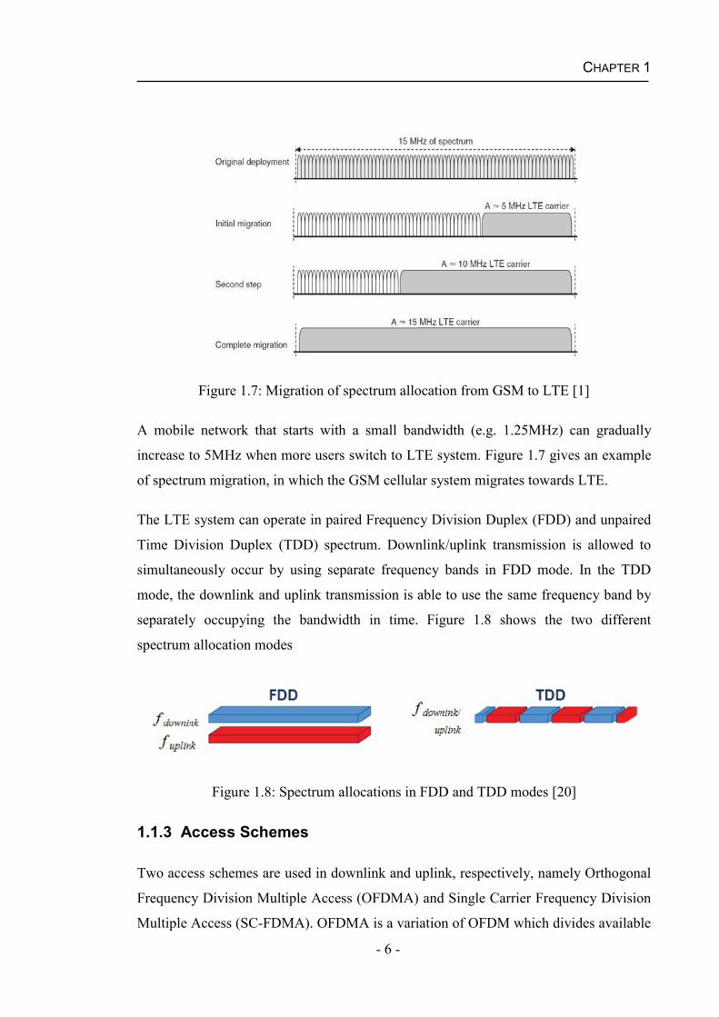
A high degree of spectrum flexibility is offered in LTE. The aim of this characteristic
allows the LTE radio access to be deployed in different sizes of the available
bandwidths, different frequency bands and different duplexities [17]. As shown in
Figure 1.6, the LTE has a wide range of transmission bandwidth from 1.25MHz up to
20MHz which depends on the available bandwidth [18]. This bandwidth availability
leads to a simple spectrum migration toward the LTE.
Figure 1.6: Scalable bandwidth in LTE [19]
CHAPTER 1
- 6 -
Figure 1.7: Migration of spectrum allocation from GSM to LTE [1]
A mobile network that starts with a small bandwidth (e.g. 1.25MHz) can gradually
increase to 5MHz when more users switch to LTE system. Figure 1.7 gives an example
of spectrum migration, in which the GSM cellular system migrates towards LTE.
The LTE system can operate in paired Frequency Division Duplex (FDD) and unpaired
Time Division Duplex (TDD) spectrum. Downlink/uplink transmission is allowed to
simultaneously occur by using separate frequency bands in FDD mode. In the TDD
mode, the downlink and uplink transmission is able to use the same frequency band by
separately occupying the bandwidth in time. Figure 1.8 shows the two different
spectrum allocation modes
Figure 1.8: Spectrum allocations in FDD and TDD modes [20]
1.1.3 Access Schemes
Two access schemes are used in downlink and uplink, respectively, namely Orthogonal
Frequency Division Multiple Access (OFDMA) and Single Carrier Frequency Division
Multiple Access (SC-FDMA). OFDMA is a variation of OFDM which divides available
CHAPTER 1
- 7 -
frequency into narrow subcarriers and allocates each user a subcarrier. The OFDMA
access technology was chosen in the downlink LTE for two main reasons: (a) to
eliminate Inter-Symbol Interference (ISI) effect caused by multipath and (b) to be
immunity to frequency-selective fading of the wireless channels [21]
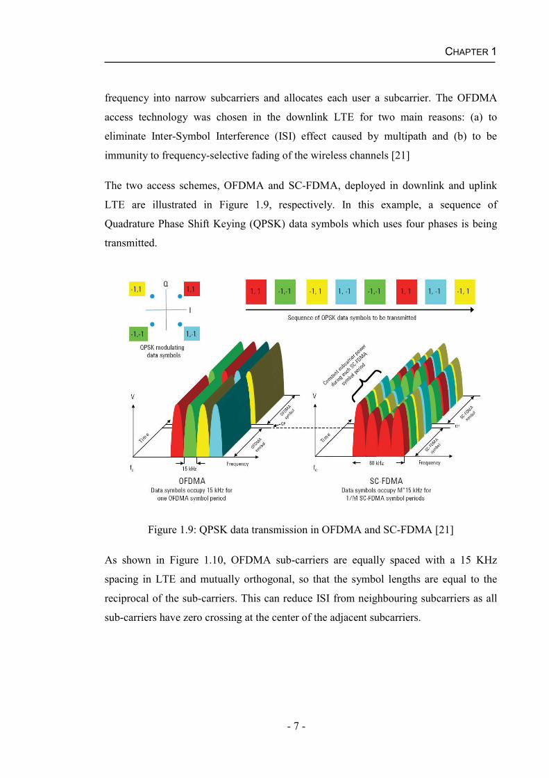
The two access schemes, OFDMA and SC-FDMA, deployed in downlink and uplink
LTE are illustrated in Figure 1.9, respectively. In this example, a sequence of
Quadrature Phase Shift Keying (QPSK) data symbols which uses four phases is being
transmitted.
Figure 1.9: QPSK data transmission in OFDMA and SC-FDMA [21]
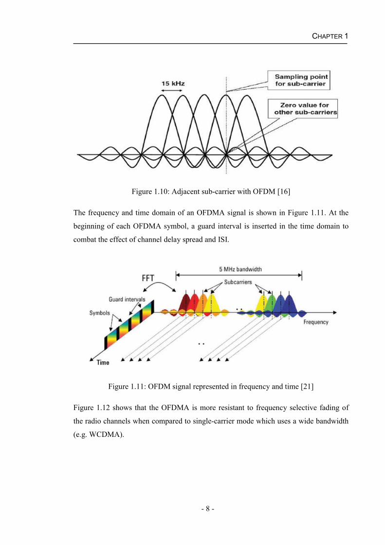
As shown in Figure 1.10, OFDMA sub-carriers are equally spaced with a 15 KHz
spacing in LTE and mutually orthogonal, so that the symbol lengths are equal to the
reciprocal of the sub-carriers. This can reduce ISI from neighbouring subcarriers as all
sub-carriers have zero crossing at the center of the adjacent subcarriers.
CHAPTER 1
- 8 -
Figure 1.10: Adjacent sub-carrier with OFDM [16]
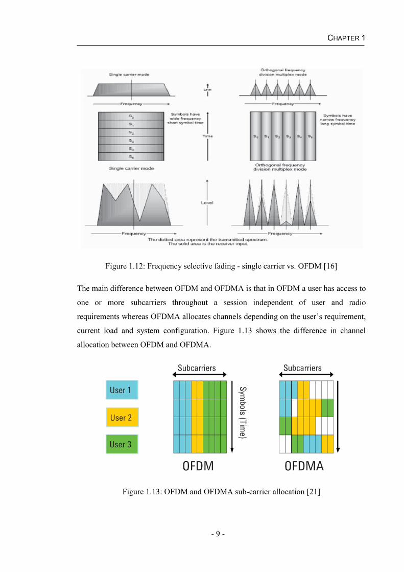
The frequency and time domain of an OFDMA signal is shown in Figure 1.11. At the
beginning of each OFDMA symbol, a guard interval is inserted in the time domain to
combat the effect of channel delay spread and ISI.
Figure 1.11: OFDM signal represented in frequency and time [21]
Figure 1.12 shows that the OFDMA is more resistant to frequency selective fading of
the radio channels when compared to single-carrier mode which uses a wide bandwidth
(e.g. WCDMA).
CHAPTER 1
- 9 -
Figure 1.12: Frequency selective fading - single carrier vs. OFDM [16]
The main difference between OFDM and OFDMA is that in OFDM a user has access to
one or more subcarriers throughout a session independent of user and radio
requirements whereas OFDMA allocates channels depending on the user’s requirement,
current load and system configuration. Figure 1.13 shows the difference in channel
allocation between OFDM and OFDMA.
Figure 1.13: OFDM and OFDMA sub-carrier allocation [21]
CHAPTER 1
- 10 -
1.1.4 Physical Resource Block (PRB)
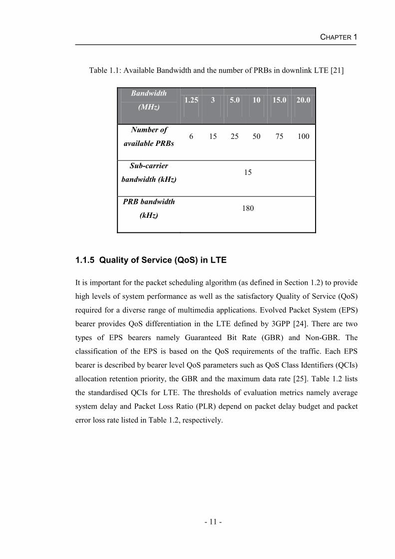
The LTE standard defines a joint time-frequency resource allocation structure. A
Resource Block (RB) defined in frequency domain has a total bandwidth of 180 kHz
which is divided into 12 consecutive sub-carriers. In time domain, the RB is defined as
a 0.5 ms time slot. A Physical Resource Block (PRB) which is the minimum allocation
unit in downlink LTE consists of two RBs. The number of OFDM symbols contained in
a PRB depends on the Cyclic Prefix (CP) type used in the OFDM symbol. When a
normal CP is used, the PRB contains 14 symbols while the PRB contains 12 symbols
for an extended CP [22]. A delay spread exceeding the normal CP length indicates the
extended CP. Figure 1.14 shows the time-frequency resource grid to represent a PRB
for the normal CP case.
Figure 1.14: PRB representation in time and frequency domains using a normal CP [23]
Each PRB is comprised of individual Resource Elements (REs) which represents one
ODFM subcarrier during one OFDM symbol interval [13]. Therefore, a total number of
168 REs are contained in each PRB if a normal CP is used. These REs are in charge of
data transmission and communication control. Table 1.1 lists the available bandwidth
and the corresponding number of PRBs in downlink LTE.
CHAPTER 1
- 11 -
Table 1.1: Available Bandwidth and the number of PRBs in downlink LTE [21]
Bandwidth
(MHz)1.25 3 5.0 10 15.0 20.0
Number of
available PRBs6 15 25 50 75 100
Sub-carrier
bandwidth (kHz)15
PRB bandwidth
(kHz)180
1.1.5 Quality of Service (QoS) in LTE
It is important for the packet scheduling algorithm (as defined in Section 1.2) to provide
high levels of system performance as well as the satisfactory Quality of Service (QoS)
required for a diverse range of multimedia applications. Evolved Packet System (EPS)
bearer provides QoS differentiation in the LTE defined by 3GPP [24]. There are two
types of EPS bearers namely Guaranteed Bit Rate (GBR) and Non-GBR. The
classification of the EPS is based on the QoS requirements of the traffic. Each EPS
bearer is described by bearer level QoS parameters such as QoS Class Identifiers (QCIs)
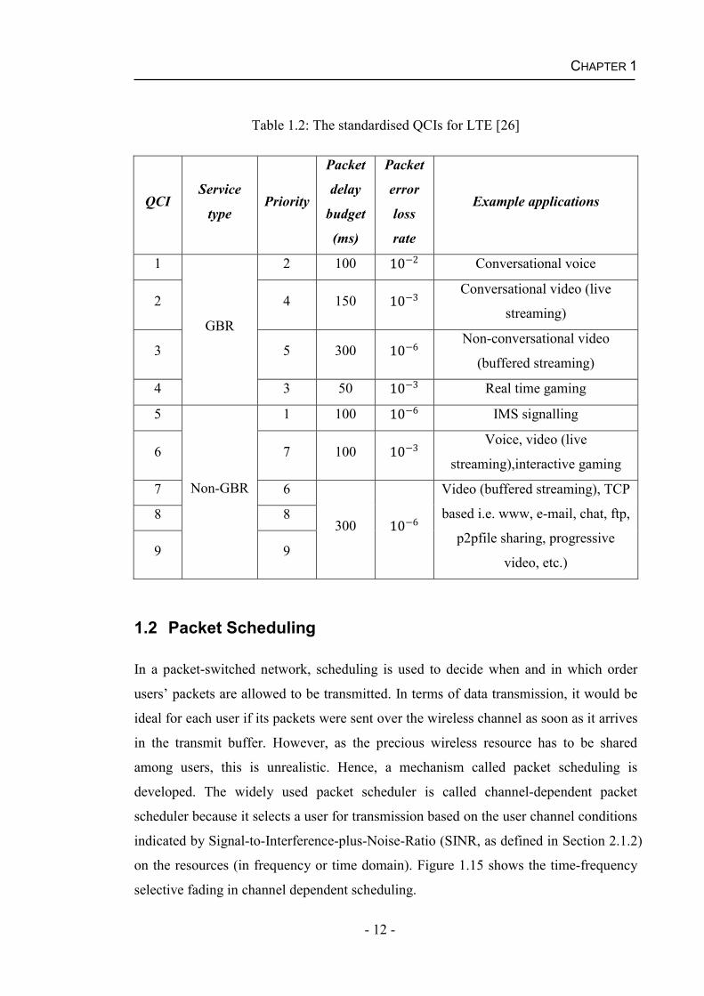
allocation retention priority, the GBR and the maximum data rate [25]. Table 1.2 lists
the standardised QCIs for LTE. The thresholds of evaluation metrics namely average
system delay and Packet Loss Ratio (PLR) depend on packet delay budget and packet
error loss rate listed in Table 1.2, respectively.
CHAPTER 1
- 12 -
Table 1.2: The standardised QCIs for LTE [26]
QCIService
typePriority
Packet
delay
budget
(ms)
Packet
error
loss
rate
Example applications
1
GBR
2 100 10 2 Conversational voice
2 4 150 10 3 Conversational video (live
streaming)
3 5 300 10 6 Non-conversational video
(buffered streaming)
4 3 50 10 3 Real time gaming
5
Non-GBR
1 100 10 6 IMS signalling
6 7 100 10 3 Voice, video (live
streaming),interactive gaming
7 6
300 10 6Video (buffered streaming), TCP
based i.e. www, e-mail, chat, ftp,
p2pfile sharing, progressive
video, etc.)
8 8
9 9
1.2 Packet Scheduling
In a packet-switched network, scheduling is used to decide when and in which order
users’ packets are allowed to be transmitted. In terms of data transmission, it would be
ideal for each user if its packets were sent over the wireless channel as soon as it arrives
in the transmit buffer. However, as the precious wireless resource has to be shared
among users, this is unrealistic. Hence, a mechanism called packet scheduling is
developed. The widely used packet scheduler is called channel-dependent packet
scheduler because it selects a user for transmission based on the user channel conditions
indicated by Signal-to-Interference-plus-Noise-Ratio (SINR, as defined in Section 2.1.2)
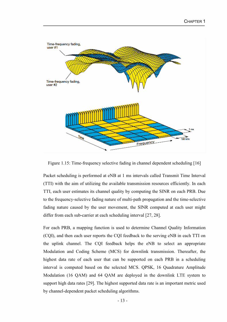
on the resources (in frequency or time domain). Figure 1.15 shows the time-frequency
selective fading in channel dependent scheduling.
CHAPTER 1
- 13 -
Figure 1.15: Time-frequency selective fading in channel dependent scheduling [16]
Packet scheduling is performed at eNB at 1 ms intervals called Transmit Time Interval
(TTI) with the aim of utilizing the available transmission resources efficiently. In each
TTI, each user estimates its channel quality by computing the SINR on each PRB. Due
to the frequency-selective fading nature of multi-path propagation and the time-selective
fading nature caused by the user movement, the SINR computed at each user might
differ from each sub-carrier at each scheduling interval [27, 28].
For each PRB, a mapping function is used to determine Channel Quality Information
(CQI), and then each user reports the CQI feedback to the serving eNB in each TTI on
the uplink channel. The CQI feedback helps the eNB to select an appropriate
Modulation and Coding Scheme (MCS) for downlink transmission. Thereafter, the
highest data rate of each user that can be supported on each PRB in a scheduling
interval is computed based on the selected MCS. QPSK, 16 Quadrature Amplitude
Modulation (16 QAM) and 64 QAM are deployed in the downlink LTE system to
support high data rates [29]. The highest supported data rate is an important metric used
by channel-dependent packet scheduling algorithms.
CHAPTER 1
- 14 -
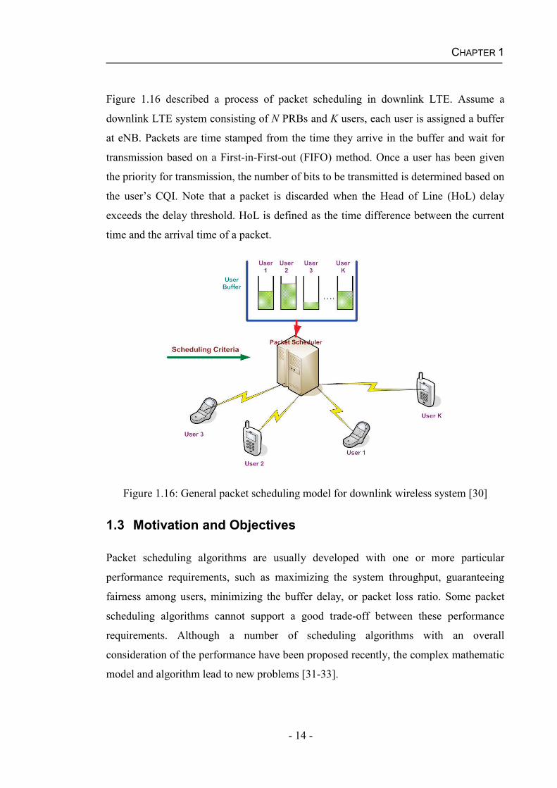
Figure 1.16 described a process of packet scheduling in downlink LTE. Assume a
downlink LTE system consisting of N PRBs and K users, each user is assigned a buffer
at eNB. Packets are time stamped from the time they arrive in the buffer and wait for
transmission based on a First-in-First-out (FIFO) method. Once a user has been given
the priority for transmission, the number of bits to be transmitted is determined based on
the user’s CQI. Note that a packet is discarded when the Head of Line (HoL) delay
exceeds the delay threshold. HoL is defined as the time difference between the current
time and the arrival time of a packet.
Figure 1.16: General packet scheduling model for downlink wireless system [30]
1.3 Motivation and Objectives
Packet scheduling algorithms are usually developed with one or more particular
performance requirements, such as maximizing the system throughput, guaranteeing
fairness among users, minimizing the buffer delay, or packet loss ratio. Some packet
scheduling algorithms cannot support a good trade-off between these performance
requirements. Although a number of scheduling algorithms with an overall
consideration of the performance have been proposed recently, the complex mathematic
model and algorithm lead to new problems [31-33].
CHAPTER 1
- 15 -
Channel-dependent scheduling of transmission of data packets in a wireless system is
based on measurement and feedback of the channel quality. However, it is unrealistic to
assume a perfect CQI report at the scheduler (transmitter) end in a practical downlink
LTE system. Because the practical imperfect channel conditions always cause a
mismatch between current channel state and the received CQI, along with the
interference, multi-path fading, and shadowing due to the unpredictable nature of
wireless channel. System performance may degrade significantly for employing a
channel-dependent packet scheduler that has continuously received inaccurate CQI
reports.
A small number of algorithms consider the performance of packet scheduling
algorithms with outdated CQI or erroneous CQI and a few algorithms consider absence
in CQI. A limited number of packet scheduling algorithms have an overall consideration
of all imperfect CQI conditions. However, due to the complex mathematical operations
that exist in these algorithms, they are not suitable for real time applications.
Given the detrimental effect of the time-varying wireless channel and the trade-off
between packet scheduling performance and complexity of scheduling algorithm, two
objectives of this thesis are given below:
Providing an overall good performance to satisfy QoS for GBR services: Is it
possible to propose a novel packet scheduling algorithm for the downlink LTE that
can offer an overall good system performance and at the same time maintain a low
computational cost? If so, how much performance improvement can the new
algorithm achieve compared to the existing packet scheduling algorithms?
Wireless environment impairments and instability: In the presence of various
practical imperfect CQI, is it possible to propose a packet scheduling algorithm
based on channel prediction with low computational complexity to adapt to all
imperfect channel states? If so, how much performance improvement can the novel
algorithm achieve compared to the existing packet scheduling algorithms?
CHAPTER 1
- 16 -
1.4 Thesis Overview
This section outlines the contributions and brief introductions of the remaining of the
thesis:
Chapter 2: Background of the Downlink LTE
This chapter introduced the background of the downlink LTE system and the simulation
models in terms of the CQI, packet scheduling and HARQ. The traffic characteristics
and performance metrics used to evaluate the packet scheduling algorithms were
presented. In addition, the simulation assumptions used throughout this thesis were
stated.
Chapter 3: Packet Scheduling Algorithms
This chapter introduces a number of packet scheduling algorithms designed in time
domain and analyzes the performance of three well-known time domain packet
scheduling algorithms in multi-carrier mobile systems. A packet scheduling algorithm is
identified that it is able to provide a better trade-off between maximizing the system
performance and guaranteeing the fairness.
Chapter 4QoS Aware Scheduling Schemes and Algorithms
In an effort to maximize the system performance without compromising the QoS
requirements, a scheme that aims to achieve the best overall performance and be robust
against the time-varying channel environments was proposed. Based on the proposed
scheme, a scheduling algorithm that classifies the whole scheduling intervals into two
groups and employs two well-known scheduling algorithms alternatively in each
interval group was proposed for GBR services.
Chapter 5 Packet Scheduling with Imperfect CQI
To overcome the severe performance degradation due to imperfect channel conditions
and provide satisfactory QoS for real time applications in the downlink LTE systems, a
novel packet scheduling algorithm was proposed in this chapter. The algorithm consists
of two parts: channel prediction and packet scheduling. The channel prediction part
CHAPTER 1
- 17 -
initially uses a channel predictor based on Kalman filter to estimate and recover correct
CQI from erroneous channel quality feedback. The packet scheduling part employs a
scheduling algorithm based on a time domain grouping scheme to make scheduling
decisions based on the estimated CQI from the channel predictor.
Chapter 6 Conclusions and Future Research Directions
The contributions made in this thesis and the recommendations of a number of future
research directions are summarized in this chapter.
1.5 Related Publications
Yongxin Wang; K. Sandrasegaran; X. Zhu; C-C Lin; A. Daeinabi, "Packet Scheduling
in LTE with Imperfect CQI" in International Journal of Advanced Research in
Computer Science and Software Engineering (IJARCSSE), Vol. 3, No. 6, July 2013, pp.
6-13.
Yongxin Wang; K. Sandrasegaran; X. Zhu; J. Fei; X. Kong; C-C Lin, "Frequency and
Time Domain Packet Scheduling Based on Channel Prediction with Imperfect CQI in
LTE" in International Journal of Wireless & Mobile Networks (IJWMN), Vol. 5, No. 4,
August 2013, pp. 157-170.
- 18 -
Chapter 2
BACKGROUND OF THE DOWNLINK LTE
In this chapter, the technical background of this research is introduced by outlining the
system model of a downlink LTE system and the characteristics of the wireless resource
allocation. A system level simulator based on C++ was used to model the LTE system
and evaluate the packet scheduling performance.
Chapter 2 begins with a general downlink LTE system model in Section 2.1. The
introductions of the CQI, packet scheduling and HARQ are presented in Section 2.2,
Section 2.3 and Section 2.4, respectively. Section 2.5 gives a thorough description of
traffic characteristics followed by discussions of four performance metrics used to
evaluate packet scheduling algorithms in Section 2.6. Section 2.7 summarises all of the
assumptions that are used in this thesis and finally, Section 2.8 concludes this chapter.
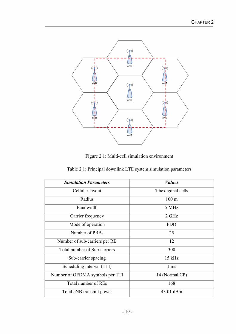
2.1 Downlink LTE System Model
A multi-cell downlink LTE system is modelled in this thesis, it contains seven
hexagonal cells and an eNodeB is located at the centre of each cell. Users are uniformly
distributed within a rectangle area as shown in Figure 2.1. A total of 43.01 dBm
eNodeB transmit power is used for downlink [34]. An LTE transmission bandwidth of 5
MHz with 25 PRBs and 2 GHz carrier frequency with normal cyclic prefix were
considered in this thesis. Table 2.1 gives a detailed summary of the main simulation
parameters in this thesis based on the LTE specifications [35].
CHAPTER 2
- 19 -
Figure 2.1: Multi-cell simulation environment
Table 2.1: Principal downlink LTE system simulation parameters
Simulation Parameters Values
Cellular layout 7 hexagonal cells
Radius 100 m
Bandwidth 5 MHz
Carrier frequency 2 GHz
Mode of operation FDD
Number of PRBs 25
Number of sub-carriers per RB 12
Total number of Sub-carriers 300
Sub-carrier spacing 15 kHz
Scheduling interval (TTI) 1 ms
Number of OFDMA symbols per TTI 14 (Normal CP)
Total number of REs 168
Total eNB transmit power 43.01 dBm
CHAPTER 2
- 20 -
2.1.1 Mobility Modelling
In this thesis, each user within the multi-cell simulation environment is initially
assigned a random location and direction and thereafter moves at a constant speed in a
constant direction throughout the data session. Three uniform user speeds are used: 3
km/h, 30 km/h and 120 km/h. The location of user i at time t is determined using
Equation (2.1): ( ) = ( 1) + ( ( 1) ( 1)) (2.1)
where ( ) is the location of user i at time t, ( 1)is the speed of user i at time 1 and ( 1) is the direction of user i at time 1.
To ensure that users always moves within the rectangle simulation area shown in Figure
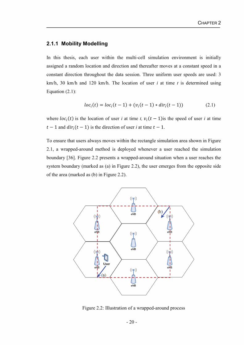
2.1, a wrapped-around method is deployed whenever a user reached the simulation
boundary [36]. Figure 2.2 presents a wrapped-around situation when a user reaches the
system boundary (marked as (a) in Figure 2.2), the user emerges from the opposite side
of the area (marked as (b) in Figure 2.2).
Figure 2.2: Illustration of a wrapped-around process
CHAPTER 2
- 21 -
2.1.2 Radio Propagation Modelling
This section describes the radio propagation modelling in terms of multi-path fading,
shadow fading, path loss and Signal-to-Interference-plus-Noise-Ratio (SINR). Radio
propagation describes the processes that affect radio signals that are transmitted from
the transmitter to receiver. It affects the strength of received signal experienced at a
receiver [37].
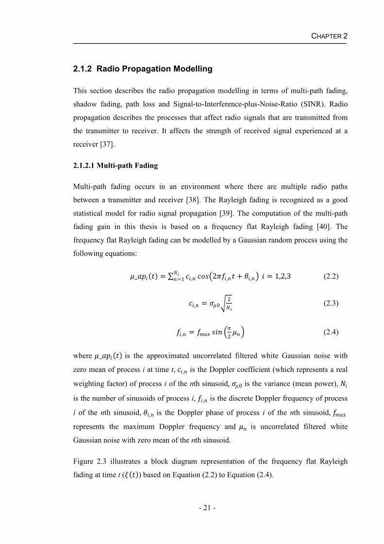
2.1.2.1 Multi-path Fading
Multi-path fading occurs in an environment where there are multiple radio paths
between a transmitter and receiver [38]. The Rayleigh fading is recognized as a good
statistical model for radio signal propagation [39]. The computation of the multi-path
fading gain in this thesis is based on a frequency flat Rayleigh fading [40]. The
frequency flat Rayleigh fading can be modelled by a Gaussian random process using the
following equations:
_ ( ) = , 2 , + , = 1,2,3=1 (2.2)
, = 0 2 (2.3)
, = 2 (2.4)
where _ ( ) is the approximated uncorrelated filtered white Gaussian noise with
zero mean of process i at time t, , is the Doppler coefficient (which represents a real
weighting factor) of process i of the nth sinusoid, 0 is the variance (mean power),
is the number of sinusoids of process i, , is the discrete Doppler frequency of process
i of the nth sinusoid, , is the Doppler phase of process i of the nth sinusoid,
represents the maximum Doppler frequency and is uncorrelated filtered white
Gaussian noise with zero mean of the nth sinusoid.
Figure 2.3 illustrates a block diagram representation of the frequency flat Rayleigh
fading at time t ( ( )) based on Equation (2.2) to Equation (2.4).
CHAPTER 2
- 22 -
Figure 2.3: Frequency flat Rayleigh fading structure [40]
2.1.2.2 Shadow Fading
Shadow fading refers to deviation of the attenuation affecting a radio signal which is
cause by reflection, diffraction and shielding from obstacles (e.g. rocks, trees and
buildings) [41]. A widely used probability distribution namely Gaussian lognormal
distribution was chosen to compute the shadow fading gain in this thesis (with 0 mean
and 8 dB standard deviation) [42]. The shadow fading gain for user i at time tis
determined by the following equations:
( ) = ( 1) ( 1) + 1 ( 1)2 ( 1) (2.5)
( 1) = ( 1)0 (2.6)
where ( 1) is the shadow fading autocorrelation function, ( 1) is a Gaussian
random variable of user i at time t-1, ( 1) is the speed of user i at time t-1, is the
shadow fading standard deviation and 0 is the shadow fading correlation distance.
2.1.2.3 Path Loss
The path loss is defined as the attenuation in power density of a radio signal when it
propagates through space [43]. It is a main component in the modelling of a wireless
CHAPTER 2
- 23 -
telecommunication system and was empirically evaluated using the Hata model for
urban environment [44]. The Hata model for urban areas is recognized as one of the
most accurate radio propagation model in wireless communications. It can be computed
using the following equations:( ) = 46.3 + 33.9 10( ) 13.82 10( ) (2.7)
( ) + 44.9 6.55 10( ) 10(| ( )|)( ) = (1.1 10( ) 0.7) (1.56 10( ) 0.8) (2.8)( ) = ( ) ( 1) (2.9)
where ( ) is the path loss (in dB) of user i at time t, | ( )| is the magnitude of
distance of user i from eNB at time t, ( ) is the location (complex number) of user i
at time t, f is the frequency of the transmission (in MHz), is the height of the eNB (in
m), is the height of the user terminal (in m) and ( ) is the mobile antenna
correction factor.
2.1.2.4 Signal-to-Interference-plus-Noise-Ratio (SINR)
Signal-to-Interference-plus-Noise-Ratio (SINR) is defined as the strength of the
received signal of interest divided by the sum of the interference and background noise.
SINR experienced by a user is time-varying on each PRB due to user mobility and
changes in the environment [28]. It was assumed in this thesis that the variation of
multi-path fading among the sub-carriers of a PRB is minimum due to a 15 kHz
subcarrier spacing. The instantaneous SINR of each user on each PRB was calculated
on a sub-carrier located at the centre frequency of the PRB [45] based on the following
equations [46]:
, ( ) = , ( )( + 0) (2.10)
, ( ) = 10 ( )10 10 ( )10 10 , ( )10 (2.11)
CHAPTER 2
- 24 -
where , ( ) is the instantaneous SINR (in dB) of user i on PRB j at time t, is the
total eNB transmit power (in dBm), ( ) is the path loss (in dB) of user i at time t,( ) is the shadow fading gain (in dB) of user i at time t, , ( ) is the multi-path
fading gain (in dB) of user i on PRB j at time t, is the maximum available
number of PRBs, 0 is the thermal noise and is the inter-cell interference. It was
assumed in this thesis that the inter-cell interference is 1 12 and remains constant
for simplicity.
2.2 Channel Quality Information (CQI)
CQI is information sent by the UE on the uplink to the eNB as an indication of received
channel quality and it is used by the packet scheduler. The instantaneous SINR
computed at a UE is mapped to a CQI value and this process is referred to as SINR-to-
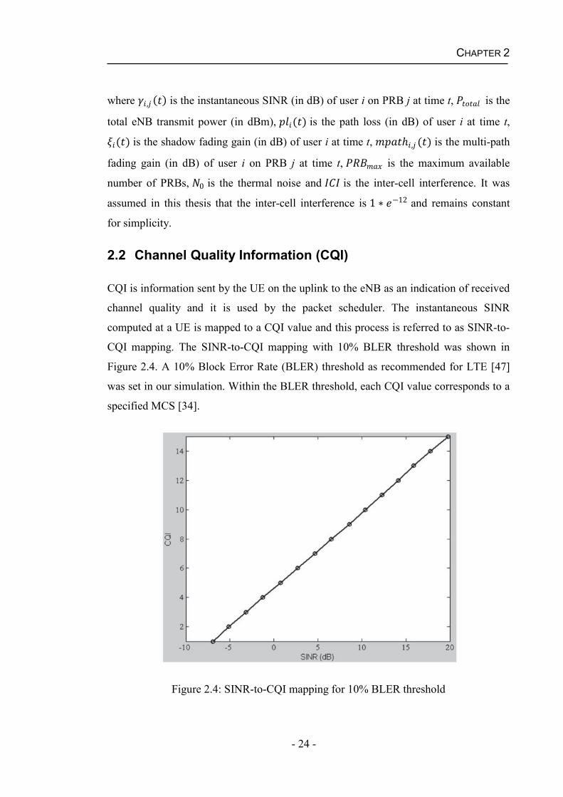
CQI mapping. The SINR-to-CQI mapping with 10% BLER threshold was shown in
Figure 2.4. A 10% Block Error Rate (BLER) threshold as recommended for LTE [47]
was set in our simulation. Within the BLER threshold, each CQI value corresponds to a
specified MCS [34].
Figure 2.4: SINR-to-CQI mapping for 10% BLER threshold
CHAPTER 2
- 25 -
It was assumed in this thesis that each user reports CQI to the eNB on each PRB at each
TTI. For simplicity, a perfect CQI reporting without delay and error is considered in
Section 3.2. Then, Section 4.4 assumed that each CQI report received by eNB has a 3
ms delay. In order to evaluate the performance of the scheduling algorithms under
imperfect CQI, some more practical assumptions were made in Chapter 5.
Besides making a scheduling decision, the CQI report is used to compute the data rate
of a user for packet transmission. Based on the data rate, the efficiency of each RE can
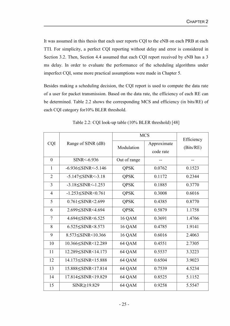
be determined. Table 2.2 shows the corresponding MCS and efficiency (in bits/RE) of
each CQI category for10% BLER threshold.
Table 2.2: CQI look-up table (10% BLER threshold) [48]
CQI Range of SINR (dB)
MCSEfficiency
(Bits/RE)ModulationApproximate
code rate
0 SINR<-6.936 Out of range -- --
1 -6.936 SINR<-5.146 QPSK 0.0762 0.1523
2 -5.147 SINR<-3.18 QPSK 0.1172 0.2344
3 -3.18 SINR<-1.253 QPSK 0.1885 0.3770
4 -1.253 SINR<0.761 QPSK 0.3008 0.6016
5 0.761 SINR<2.699 QPSK 0.4385 0.8770
6 2.699 SINR<4.694 QPSK 0.5879 1.1758
7 4.694 SINR<6.525 16 QAM 0.3691 1.4766
8 6.525 SINR<8.573 16 QAM 0.4785 1.9141
9 8.573 SINR<10.366 16 QAM 0.6016 2.4063
10 10.366 SINR<12.289 64 QAM 0.4551 2.7305
11 12.289 SINR<14.173 64 QAM 0.5537 3.3223
12 14.173 SINR<15.888 64 QAM 0.6504 3.9023
13 15.888 SINR<17.814 64 QAM 0.7539 4.5234
14 17.814 SINR<19.829 64 QAM 0.8525 5.1152
15 SINR 19.829 64 QAM 0.9258 5.5547
CHAPTER 2
- 26 -
A PRB using normal cyclic prefix contains 168 resource elements as discussed in
Chapter 1. It was assumed in this work that a PRB has 148 resource elements (RE) for
10% BLER threshold and 20 REs are used for control and signalling purposes [34]. The
instantaneous data rate can be computed based on the CQI look-up table (see Table 2.2)
and the total number of REs specified for downlink data transmission, the mathematical
expression of the instantaneous data rate of each user is given below:
, ( ) = , ( ) (2.12)
where , ( ) is the instantaneous data rate of user i on PRB j at time t, , ( )is the efficiency (Column 5 in Table 2.2) of PRB j of user i at time t, is the total
number of REs specified for downlink data transmission and TTI represents the current
scheduling interval.
2.3 Packet Scheduling
User data for downlink transmission are segmented into smaller packets of fixed size,
time-stamped and stored in the buffer at the eNB. When a packet arrives at the eNB
buffer, a timer is started and the packets whose delay exceeds the buffer delay threshold
(20 ms is set for GBR services throughout this thesis) will be discarded. The packet
delay is defined as the duration from the time a packet arrives in the buffer until current
time t. Equation (2.13) is its mathematical expression.
, ( ) = , (2.13)
where , ( ) is the delay of the lth packet of user i at time t and , is the time of
arrival of the lth packet of user i in the eNB buffer.
In each scheduling interval and on each PRB, a user with the highest priority is selected
for packet transmission. A user may be assigned more than one PRB in each scheduling
interval but each PRB can only be allocated to a single user in each scheduling interval
in the downlink LTE.
A Transport Block (TB) is defined as a group of packets that are transmitted from the
scheduler to a user in a scheduling interval. Each TB is assigned a unique Transmission
CHAPTER 2
- 27 -
Sequence Number (TSN) which is used by the user for in sequence delivery of packets
towards the higher layers [49]. To ensure a reliable delivery, Cyclic Redundancy Check
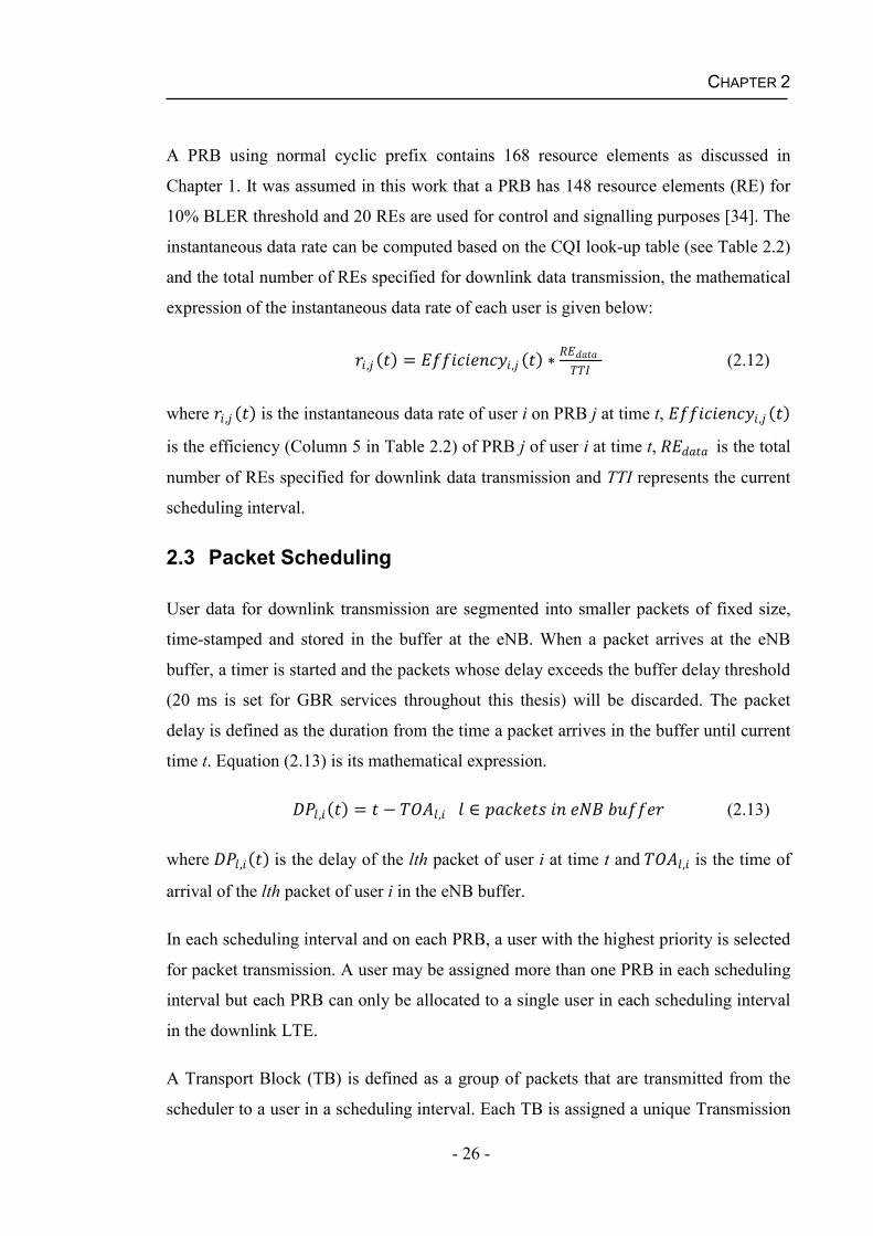
(CRC) bits are inserted in each TB for error-detection. Figure 2.5 illustrates a TB
structure with a number of packets and CRC bits. The size of a TB is determined by the
corresponding MCS of the user on each PRB. A higher MCS indicates a better
transmission capacity. The data rate of the packet is dependent on the size of the TB.
Figure 2.5: A TB structure diagram [23]
In each scheduling interval, packets are queued in the eNB buffer upon transmission
[50-52] and removed from the buffer when:
i) a positive Acknowledgement (ACK) feedback associated with the TB is received
ii) the number of retransmission has exceeded the pre-defined maximum value if
Hybrid Automatic Repeat Request (HARQ) technique is enabled.
iii) a Radio Link Control (RLC) feedback that indicates the expiry of re-sequencing
timer is received.
Note that once there is one packet of a TB exceeding the buffer delay threshold, all
packets of the TB are discarded from the eNB buffer.
2.4 Hybrid Automatic Repeat Request (HARQ)
HARQ technique is a combination of Forward Error Correction (FEC) and Automatic
Repeat Request (ARQ) [53]. Each TB is encoded prior to (re)transmission [54] and
decoded at the user end by checking the CRC bits. If the TB is decoded correctly the
CHAPTER 2
- 28 -
user sends an ACK feedback to the eNB. Otherwise, a Negative Acknowledgement
(NACK) indicating a failed decoding and a request for retransmission is sent to the eNB.
The simplest version of HARQ is referred to as Type I HARQ. The erroneous TB is
discarded by the user in Type I HARQ. A more sophisticated version is referred to as
Type II HARQ and the erroneous TB is stored in the user’s buffer and waits for
comparison with subsequent retransmission(s).
In addition, Type II HARQ consists of two widely used techniques: (a) Chase
Combining (CC) [55] and (b) Incremental Redundancy (IR) [56]. In the CC technique,
the retransmission TB is identical to the initial transmission because it is transmitted
with the same MCS and the same number of PRBs. The retransmitted TB is combined
with previously received TB(s) that have the same TSN at the receiver end. In this
thesis, the CC HARQ technique was used in the simulation.
In the IR HARQ method, multiple versions of a TB are generated each with different
combination of systematic bits and parity bits. In each retransmission, a new version of
the TB is sent to the user. The IR technique allows different MCSs for each
retransmission. The efficiency of decoding and transmission of packets can benefit from
combining multiple retransmissions.
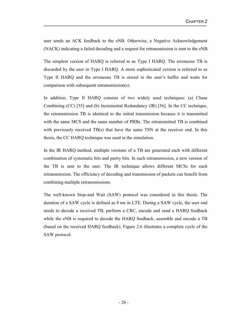
The well-known Stop-and Wait (SAW) protocol was considered in this thesis. The
duration of a SAW cycle is defined as 8 ms in LTE. During a SAW cycle, the user end
needs to decode a received TB, perform a CRC, encode and send a HARQ feedback
while the eNB is required to decode the HARQ feedback, assemble and encode a TB
(based on the received HARQ feedback). Figure 2.6 illustrates a complete cycle of the
SAW protocol.
CHAPTER 2
- 29 -
Figure 2.6:A complete cycle of the SAW protocol [57]
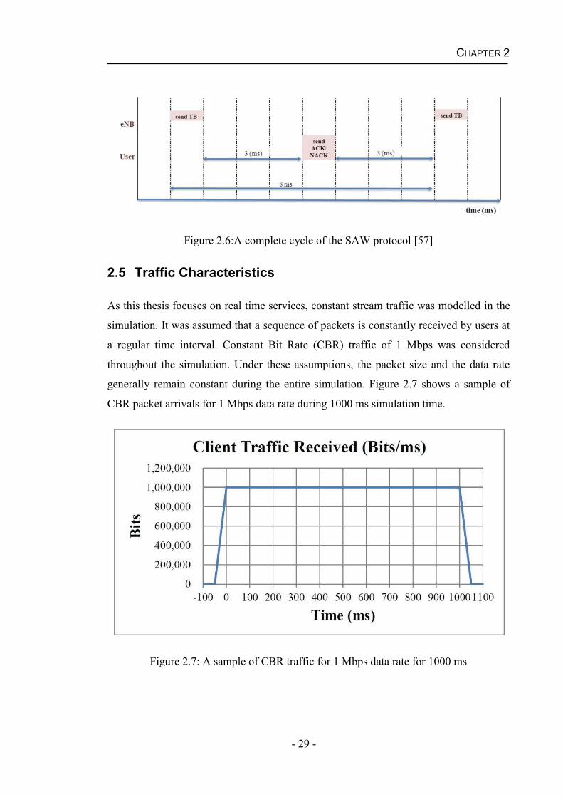
2.5 Traffic Characteristics
As this thesis focuses on real time services, constant stream traffic was modelled in the
simulation. It was assumed that a sequence of packets is constantly received by users at
a regular time interval. Constant Bit Rate (CBR) traffic of 1 Mbps was considered
throughout the simulation. Under these assumptions, the packet size and the data rate
generally remain constant during the entire simulation. Figure 2.7 shows a sample of
CBR packet arrivals for 1 Mbps data rate during 1000 ms simulation time.
Figure 2.7: A sample of CBR traffic for 1 Mbps data rate for 1000 ms
CHAPTER 2
- 30 -
2.6 Performance Metrics
Four important metrics are used in this thesis to evaluate the performance of a packet
scheduler namely system throughput, Packet Loss Ratio (PLR), fairness and average
system queuing delay.
System throughput is defined as the total data rate for successfully delivered packets to
all users in a mobile cellular system [58]. It is expressed in this thesis as the ratio of the
total size of correctly received packets (in bits) for all users to the simulation time. The
system throughput is mathematically expressed as follows:
= 1 ( )=1=1 (2.14)
where ( ) is the total size of correctly received packets (in bits) of user i at time t, T
is the simulation time and N is the total number of users.
A packet is discarded if the packet delay exceeds the delay tolerance of the system. The
PLR metric represents the percentage of discarded packets. The PLR is defined as the
total size of discarded packets divided by the total size of all packets that have resided in
the eNB buffer. Real time (RT) and Non real time (NRT) services have different PLR
thresholds as shown in Table 1.2. The following equation gives the mathematical
expression of PLR:
= ( )=1=1 ( )=1=1 (2.15)
where PLR is the packet loss ratio and ( ) represents the total size of
discarded packets (in bits) of user i at time t. ( ) is the total size of all packets (in
bits) that have arrived into the eNB buffer of user i at time t, N is the total number of
users and T is the total simulation time.
Fairness is generally defined as the difference between users that receive the maximum
and the minimum performance (i.e. in terms of packet transmission time, throughput,
delay, etc.) [59]. In this thesis, fairness is computed by the difference in the total size of
transmitted packets between the most and the least served users based on a given
algorithm over a given time frame [60]. The higher the fairness of an algorithm has, the
CHAPTER 2
- 31 -
less the difference in receiving/transmitting packets between users. The mathematical
expression for the fairness is given below:
= 1 ( )=1 ( ( )=1 )( )=1=1 (2.16)
where ( ) is the total size of received packets (in bits) of user i at time t, ( )is the total size of all packets that have arrived to the eNB buffer of user i at time t, N is
the total number of users and T is the total simulation time.
The average system queuing delay is defined as the average of the total packet delay of
all packets in the eNB buffer. In order to improve the system performance, the average
system queuing delay needs to be kept at the minimum. In this thesis, the average
system queuing delay is equal to the average delay of HoL packets (as defined in
Section 1.2) of all users for the entire simulation time. The HoL packet of a user can be
mathematically expressed using Equation (2.17).
( ) = , ( ) (2.17)
where ( ) is the delay of the HoL packet of user i at time t and , ( ) is the delay
of the lth packet of user i at time t.
Equation (2.18) gives the mathematical expression of the average system queuing delay.
= 1 1=1 ( )=1 (2.18)
where ( ) is the delay of the HoL packet of user i at time t (as defined in Equation
(2.17)), is the total number of users and is the total simulation time.
2.7 Summary of Assumptions
This section presents all of the simulation assumption details throughout the thesis.
A user is wrapped-around whenever it reaches the system boundary and an equal and
constant user speed was considered throughout a simulation. Two user speed scenarios
are compared in Section 4.4 and Chapter 5 (i.e. 3 km/h and 30 km/h), respectively,
while a single user speed scenario (i.e. 30 km/h) was assumed in Section 3.2. The
CHAPTER 2
- 32 -
instantaneous SINR on a PRB was calculated on a sub-carrier located at the centre
frequency of the PRB as there are minimum variations of multi-path fading among the
sub-carriers of a PRB [23]. Inter-cell interference is assumed to be constant. Frequency
reuse factor is set to 1.
The CQI was reported to the eNB on each PRB at each scheduling interval. Section 3.2
assumed an error-free and delay-free CQI report while a 3 ms delay was considered in
each CQI report in Section 4.4. A more practical channel condition was applied in
Section 5.4 where all the CQI report had a 3 ms delay and became unavailable at a
regular interval (10 ms). When an up-to-date CQI is unavailable, the eNB uses the latest
received CQI.
2.8 Summary
This chapter introduced the background of the downlink LTE system and the simulation
model in terms of the mobility modelling and radio propagation modelling. The
concepts and the simulation assumptions of the CQI, packet scheduling and HARQ
were discussed. A CBR traffic model for GBR applications was presented. Four widely
used performance metrics were defined in this chapter to evaluate the packet scheduling
algorithms. Finally, the simulation assumptions throughout this thesis were outlined.
- 33 -
Chapter 3
PACKET SCHEDULING ALGORITHMS
Packet scheduling is one of the key features of the Radio Resource Management (RRM)
in the LTE systems as it allocates available radio resources at each time instant among
users for transmission so as to satisfy their QoS requirements.
The LTE standard defines a resource allocation in time and frequency domains (as
previously discussed in Chapter 1), this feature encourages the use of both time and
frequency domain packet scheduling algorithms. Some metrics considered by Time
Domain (TD) packet schedulers such as average data rate, packet delay information can
be further applied and generalized to Frequency Domain (FD) packet schedulers for
downlink LTE system.
This chapter first introduces a number of time domain packet scheduling algorithms.
Some of the algorithms prioritize users based on CQI value such as Maximum Rate
(Max-Rate) algorithm, Proportional Fair (PF) algorithm, Modified-Largest Weighted
Delay First (M-LWDF) algorithm and Exponential Rule (EXP) algorithm. Some of the
algorithms calculate the priority of scheduling based on the buffer state, for example,
Delay Prioritized Scheduling (DPS) algorithm and Maximum Laxity First (MLF)
algorithm. Then the performance of three well-known time domain packet scheduling
algorithms, Round Robin (RR) [1], Proportional Fair (PF) [61] and Delay Prioritized
Scheduling (DPS) [62] algorithms, are evaluated in a multi-carrier LTE system.
This chapter is organized as follows: Section 3.1 gives a detailed description of the time
domain packet scheduling algorithms. Section 3.2 analyzes and discusses the
performance of RR, PF and DPS algorithms for real time traffic in the downlink LTE
based on the simulation results. Finally, a summary of this chapter is given in Section
3.3.
CHAPTER 3
- 34 -
3.1 Time Domain Packet Scheduling Algorithms
The following sub-sections describe a number of packet scheduling algorithms
developed in time domain.
3.1.1 Round Robin (RR) Algorithm
Fairness is an important designing aim considered by scheduling algorithms, especially
when a fair allocation of subcarriers is necessary.
Round Robin is one representative packet scheduling algorithm that has a good fairness
performance as it selects users in turn for transmission to ensure that each active user
could receive the equal transmission resource. Due to the fact that RR algorithm does
not take into account any channel conditions, the radio resources are equally assigned to
each user regardless of its channel quality, therefore the system throughput will not be
able to be optimized.
3.1.2 Maximum Rate (Max-Rate) Algorithm
A number of packet scheduling algorithms were introduced to exploit the property of
time-varying mobile cellular channels aiming to maximize the system throughput. One
example is Maximum Rate (Max-Rate) algorithm. As the name suggests, the Max-Rate
[63] algorithm always selects a user with the best channel quality on a radio resource for
transmission. Despite better system throughput, it may not guarantee a fair treatment
among the users since it simply exploits favourable channel conditions and rarely gives
any chance to a user that experiences consistently poor channel conditions. In each
scheduling interval, this algorithm schedules a user that maximizes metric ( ) in
Equation (3.1). ( ) = ( ) (3.1)
where ( ) is the priority of user i at scheduling interval t, ( ) is the instantaneous
datarate (across the whole bandwidth) of user i at scheduling interval t.
CHAPTER 3
- 35 -
3.1.3 Proportional Fair (PF) Algorithm
To provide an attractive trade-off between throughput maximisation and fairness
guarantee, PF algorithm [61]was developed for High Data Rate (HDR) networks. The
design objective of PF algorithm is to maximize the long term throughput of the user
whose current achievable data rate is better compared to the average throughput of the
user [64].
However, due to the lack of consideration of each user’s buffer information such as the
delay of the HoL packet, the PF scheduling algorithm is unlikely to support real time
services. The PF algorithm schedules packets of a user in each time scheduling interval
as expressed in Equation (3.2), Equation (3.3), and Equation (3.4).
( ) = ( )( ) (3.2)
( + 1) = 1 1 ( ) + ( + 1) 1 ( + 1) (3.3)
( + 1) = 1 + 10 + 1 (3.4)
where ( ) is the priority of user i at scheduling interval t, ( ) is the instantaneous
datarate (across the whole bandwidth) of user i at scheduling interval t, ( ) is the
average throughput of user i at scheduling interval t, ( + 1) is the indicator function
of the eventthat packets of user i are selected for transmission at scheduling interval t+1
and is atime constant.
3.1.4 Blind Equal Throughput (BET) Algorithm
Blind Equal Throughput (BET) [65] algorithm is a well-known channel unaware packet
scheduling algorithm which was investigated based on the LTE system to provide
effective fairness. Throughput fairness can be optimized with the BET algorithm as it
stores the past average throughput achieved by each user and attempts to ensure a fair
allocation of it among users. In each scheduling interval, the BET algorithm selects a
user with the highest priority metric ( ) in Equation (3.5):
CHAPTER 3
- 36 -
( ) = 1( ) (3.5)
where ( ) is the priority of user i at scheduling interval t, ( ) is the average
throughput of user i at scheduling interval t. Equation (3.3) is used to update ( ).
3.1.5 Delay Prioritized Scheduling (DPS) Algorithm
For real time applications, packet scheduling may prioritize packets that are close to
their specified delay deadlines. In [62], a simple scheduling algorithm known as Delay
Prioritised Scheduling (DPS) algorithm that takes only the packet delay information into
account was developed. The DPS algorithm serves a user whose packets are
approaching the buffer delay threshold so as to provide satisfactory QoS needs of the
GBR services in the downlink LTE. ( ) = ( ) (3.6)
where ( ) is the time to live of the HoL packet of user i at TTI t, is the service-
dependent buffer delay threshold of user i and ( ) is the delay of the HoL packet of
user i at TTI t.
3.1.6 Maximum Laxity First (MLF) Algorithm
MLF algorithm [66] is developed for real time services. MLF algorithm is performed
based on calculating users’ priorities according to their delay deadline and remaining
execution time (execution time is referred to the time consumed in responding to a
control signal). The precise remaining execution time is unknown at each scheduling
interval which needs to be estimated by the algorithm. However, an incorrect estimation
of execution time could lead to performance degradation. The MLF algorithm schedules
a user with minimum ( ) as expressed below:( ) = ( ) ( ) (3.7)
where ( ) is laxity time of user i at TTI t, ( ) is the time to live of the HoL packet
of user i at TTI t (see Equation (3.6)), ( ) is the execution time of user i at TTI t.
CHAPTER 3
- 37 -
3.1.7 Modified-Largest Weighted Delay First (M-LWDF) Algorithm
In order to support QoS of multiple real time data users sharing a wireless channel, M-
LWDF [57] algorithm was proposed. This algorithm is based on an overall
consideration of packet delay information, the instantaneous data rate and average
throughput and is expected to have a reasonably good overall performance. The M-
LWDF algorithm selects a user that maximizes metric ( ) in Equation (3.8) to receive
its packet in each scheduling interval.
( ) = ( ) ( )( ) (3.8)
= ( ) (3.9)
where ( ) is the priority of user i at scheduling interval t, is the QoS requirement of
user i, ( ) is the delay of the HoL packet (as defined in Section 1.2) of user i at
scheduling interval t, ( ) represents the instantaneous data rate (across the whole
bandwidth) of user i at scheduling interval t and ( ) is the average throughput of user
i at scheduling interval t (as defined in Equation (3.3)). In addition, indicates the
service-dependent PLR threshold of user i and is the service-dependent buffer delay
threshold of user i.
3.1.8 Exponential Rule (EXP) Algorithm
A scheduling algorithm called Exponential Rule (EXP) algorithm was developed in [67]
to support real time and non-real time services over HDR/CDMA system. The EXP
algorithm selects a user that maximizes metric ( ) in Equation (3.10) to receive its
packets in each scheduling interval.
( ) = ( ) ( )( ) ( ( ) _1+ _ ) (3.10)
_ = 1 ( )==1 (3.11)
where ( ) is the priority of user i at scheduling interval t, is the QoS requirement of
user i (see Equation (3.9)), ( ) is the delay of the HoL packet of user i at scheduling
CHAPTER 3
- 38 -
interval t, ( ) represents the instantaneous data rate (across the whole bandwidth) of
user i at scheduling interval t, ( ) is the average throughput of user i at scheduling
interval t (as defined in Equation (3.3)) and N is the total number of users.
3.2 Performance of the FD DPS, PF and RR Algorithms for Real time Services
This section analyses and compares the performance of the DPS, PF, and RR algorithms
in terms of system throughput, PLR, fairness and average system queuing delay. The
three well-known time domain packet scheduling algorithms described in this chapter
were originally designed for single carrier cellular systems. Since time domain only
schedulers simply allocate all resources to a single user in one TTI, some modifications
need to be made to adapt it to the multi-carrier downlink LTE systems.
The adaptations made to time domain DPS, PF and RR algorithms are introduced in
Section 3.2.1. Then, results and analysis of the performances are provided in Section
3.2.2.
3.2.1 Adaptation of Selected Packet Scheduling Algorithms in the Downlink LTE
In a single carrier system, the selected user has full access to all radio resources in one
scheduling interval. In a multi-carrier system, users compete for the shared PRBs in
each TTI, the user who has the highest priority on the PRB can be assigned the resource.
A user may have the highest priority on a number of PRBs therefore all these PRBs
could be allocated to the user but each PRB can only be assigned to one user in each
TTI. In order to adapt to multi-carrier downlink LTE, the DPS, PF, and RR algorithms
are modified as below.
3.2.1.1 Delay Prioritized Scheduling (DPS) Algorithm
The multi-carrier DPS algorithm consists of four steps in one scheduling interval. In
Step 1, it calculates the delay of the HoL packet of each user using Equation (3.6). In
Step 2, the multi-carrier DPS algorithm sorts all users based on their HoL delay in
ascending order and selects a user with the least time to live in the buffer. Thereafter, a
CHAPTER 3
- 39 -
PRB with the best channel condition is assigned to the user and the assigned PRB is
removed from a list of allocatable PRBs in Step 3. Step 4 updates the HoL delay of the
remaining packets. Step 2 to Step 4 are repeated until the all the remaining PRBs have
been assigned to users or all users have been given a sufficient number of PRBs.
3.2.1.2 Proportional Fair (PF) Algorithm
The multi-carrier PF algorithm schedules a user with maximum metric , ( ) for
transmission on PRB j at TTI t as expressed in Equation (3.12).
, ( ) = , ( )( ) (3.12)
( + 1) = 1 1 ( ) + 1 ( + 1) (3.13)
( + 1) = , ( + 1)=1 , ( + 1) (3.14)
, ( + 1) = 1 + 10 + 1(3.15)
where , ( ) is the priority of user i on PRB j at TTI t, , ( ) is the instantaneous data
rate of user i on PRB j at TTI t, ( ) is the average throughput of user i at TTI t, is a
time constant, ( + 1) is the total data rate being used to transmit packets to user i
at TTI t+1. , ( + 1) is the indicator function of the eventthat packets of user i are
selected for transmission on PRB j at TTI t+1 and is the maximum available
number of PRBs.
3.2.1.3 Round Robin (RR) Algorithm
The multi-carrier RR algorithm selects active users on each PRB in turn for
transmission in each scheduling interval.
3.2.2 Performance of the Real time Service with Increasing System Capacity
This section evaluates the performance of the multi-carrier DPS, PF and RR algorithms
(for simplicity, they are hereinafter referred to as the DPS, PF and RR algorithms,
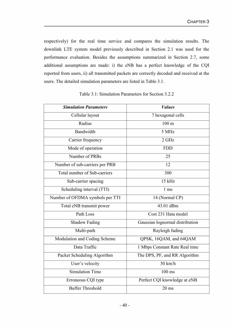
CHAPTER 3
- 40 -
respectively) for the real time service and compares the simulation results. The
downlink LTE system model previously described in Section 2.1 was used for the
performance evaluation. Besides the assumptions summarized in Section 2.7, some
additional assumptions are made: i) the eNB has a perfect knowledge of the CQI
reported from users, ii) all transmitted packets are correctly decoded and received at the
users. The detailed simulation parameters are listed in Table 3.1.
Table 3.1: Simulation Parameters for Section 3.2.2
Simulation Parameters Values
Cellular layout 7 hexagonal cells
Radius 100 m
Bandwidth 5 MHz
Carrier frequency 2 GHz
Mode of operation FDD
Number of PRBs 25
Number of sub-carriers per PRB 12
Total number of Sub-carriers 300
Sub-carrier spacing 15 kHz
Scheduling interval (TTI) 1 ms
Number of OFDMA symbols per TTI 14 (Normal CP)
Total eNB transmit power 43.01 dBm
Path Loss Cost 231 Hata model
Shadow Fading Gaussian lognormal distribution
Multi-path Rayleigh fading
Modulation and Coding Scheme QPSK, 16QAM, and 64QAM
Data Traffic 1 Mbps Constant Rate Real time
Packet Scheduling Algorithm The DPS, PF, and RR Algorithm
User’s velocity 30 km/h
Simulation Time 100 ms
Erroneous CQI type Perfect CQI knowledge at eNB
Buffer Threshold 20 ms
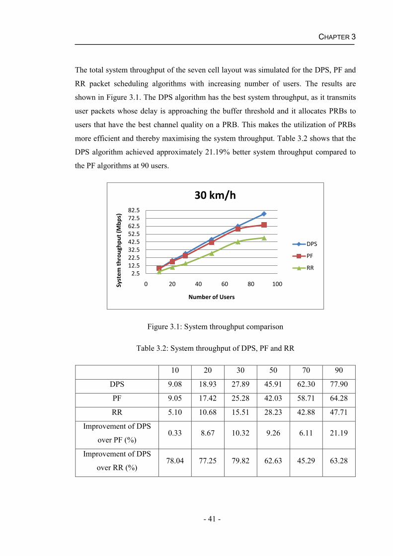
CHAPTER 3
- 41 -
The total system throughput of the seven cell layout was simulated for the DPS, PF and
RR packet scheduling algorithms with increasing number of users. The results are
shown in Figure 3.1. The DPS algorithm has the best system throughput, as it transmits
user packets whose delay is approaching the buffer threshold and it allocates PRBs to
users that have the best channel quality on a PRB. This makes the utilization of PRBs
more efficient and thereby maximising the system throughput. Table 3.2 shows that the
DPS algorithm achieved approximately 21.19% better system throughput compared to
the PF algorithms at 90 users.
Figure 3.1: System throughput comparison
Table 3.2: System throughput of DPS, PF and RR
10 20 30 50 70 90
DPS 9.08 18.93 27.89 45.91 62.30 77.90
PF 9.05 17.42 25.28 42.03 58.71 64.28
RR 5.10 10.68 15.51 28.23 42.88 47.71
Improvement of DPS
over PF (%)0.33 8.67 10.32 9.26 6.11 21.19
Improvement of DPS
over RR (%)78.04 77.25 79.82 62.63 45.29 63.28
2.512.522.532.542.552.562.572.582.5
0 20 40 60 80 100Syst
em t
hrou
ghpu
t (M
bps)
Number of Users
30 km/h
DPS
PF
RR
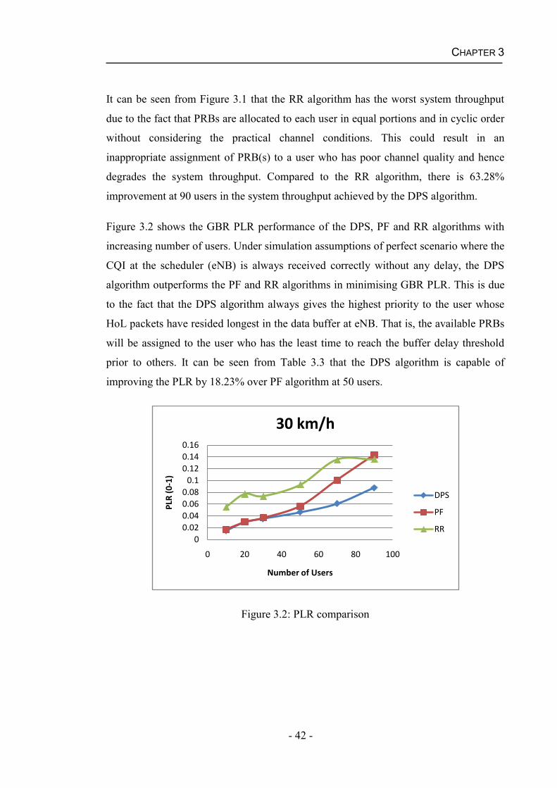
CHAPTER 3
- 42 -
It can be seen from Figure 3.1 that the RR algorithm has the worst system throughput
due to the fact that PRBs are allocated to each user in equal portions and in cyclic order
without considering the practical channel conditions. This could result in an
inappropriate assignment of PRB(s) to a user who has poor channel quality and hence
degrades the system throughput. Compared to the RR algorithm, there is 63.28%
improvement at 90 users in the system throughput achieved by the DPS algorithm.
Figure 3.2 shows the GBR PLR performance of the DPS, PF and RR algorithms with
increasing number of users. Under simulation assumptions of perfect scenario where the
CQI at the scheduler (eNB) is always received correctly without any delay, the DPS
algorithm outperforms the PF and RR algorithms in minimising GBR PLR. This is due
to the fact that the DPS algorithm always gives the highest priority to the user whose
HoL packets have resided longest in the data buffer at eNB. That is, the available PRBs
will be assigned to the user who has the least time to reach the buffer delay threshold
prior to others. It can be seen from Table 3.3 that the DPS algorithm is capable of
improving the PLR by 18.23% over PF algorithm at 50 users.
Figure 3.2: PLR comparison
00.020.040.060.08
0.10.120.140.16
0 20 40 60 80 100
PLR
(0-1
)
Number of Users
30 km/h
DPS
PF
RR
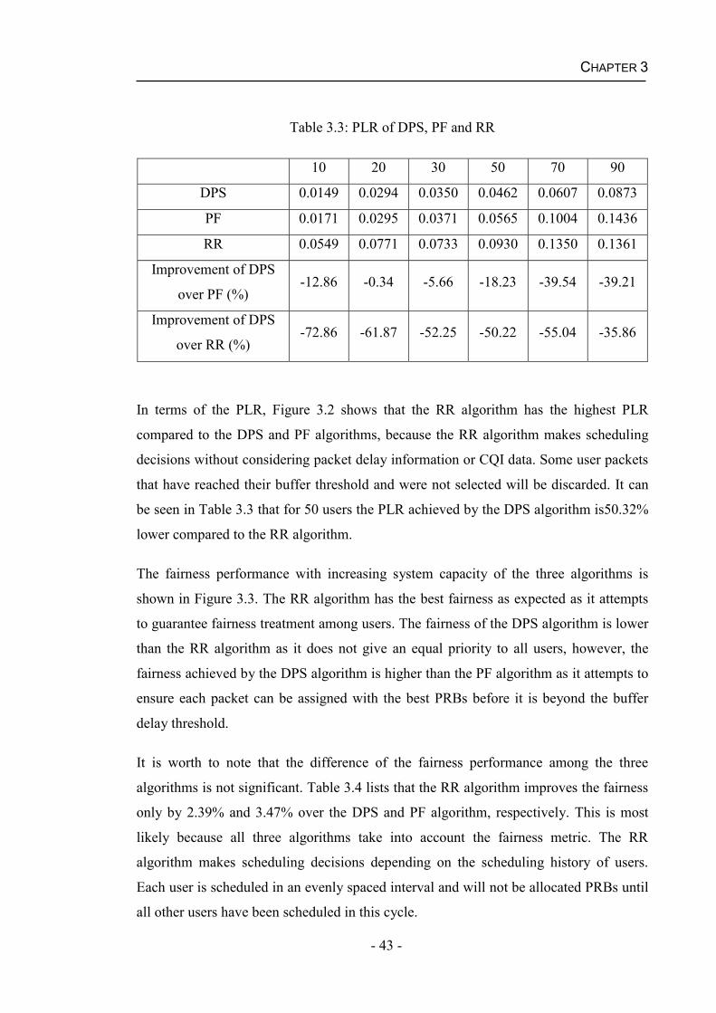
CHAPTER 3
- 43 -
Table 3.3: PLR of DPS, PF and RR
10 20 30 50 70 90
DPS 0.0149 0.0294 0.0350 0.0462 0.0607 0.0873
PF 0.0171 0.0295 0.0371 0.0565 0.1004 0.1436
RR 0.0549 0.0771 0.0733 0.0930 0.1350 0.1361
Improvement of DPS
over PF (%)-12.86 -0.34 -5.66 -18.23 -39.54 -39.21
Improvement of DPS
over RR (%)-72.86 -61.87 -52.25 -50.22 -55.04 -35.86
In terms of the PLR, Figure 3.2 shows that the RR algorithm has the highest PLR
compared to the DPS and PF algorithms, because the RR algorithm makes scheduling
decisions without considering packet delay information or CQI data. Some user packets
that have reached their buffer threshold and were not selected will be discarded. It can
be seen in Table 3.3 that for 50 users the PLR achieved by the DPS algorithm is50.32%
lower compared to the RR algorithm.
The fairness performance with increasing system capacity of the three algorithms is
shown in Figure 3.3. The RR algorithm has the best fairness as expected as it attempts
to guarantee fairness treatment among users. The fairness of the DPS algorithm is lower
than the RR algorithm as it does not give an equal priority to all users, however, the
fairness achieved by the DPS algorithm is higher than the PF algorithm as it attempts to
ensure each packet can be assigned with the best PRBs before it is beyond the buffer
delay threshold.
It is worth to note that the difference of the fairness performance among the three
algorithms is not significant. Table 3.4 lists that the RR algorithm improves the fairness
only by 2.39% and 3.47% over the DPS and PF algorithm, respectively. This is most
likely because all three algorithms take into account the fairness metric. The RR
algorithm makes scheduling decisions depending on the scheduling history of users.
Each user is scheduled in an evenly spaced interval and will not be allocated PRBs until
all other users have been scheduled in this cycle.
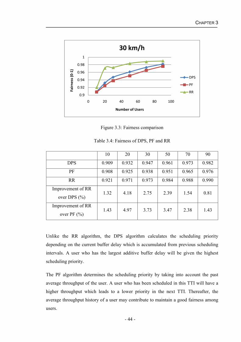
CHAPTER 3
- 44 -
Figure 3.3: Fairness comparison
Table 3.4: Fairness of DPS, PF and RR
10 20 30 50 70 90
DPS 0.909 0.932 0.947 0.961 0.973 0.982
PF 0.908 0.925 0.938 0.951 0.965 0.976
RR 0.921 0.971 0.973 0.984 0.988 0.990
Improvement of RR
over DPS (%)1.32 4.18 2.75 2.39 1.54 0.81
Improvement of RR
over PF (%)1.43 4.97 3.73 3.47 2.38 1.43
Unlike the RR algorithm, the DPS algorithm calculates the scheduling priority
depending on the current buffer delay which is accumulated from previous scheduling
intervals. A user who has the largest additive buffer delay will be given the highest
scheduling priority.
The PF algorithm determines the scheduling priority by taking into account the past
average throughput of the user. A user who has been scheduled in this TTI will have a
higher throughput which leads to a lower priority in the next TTI. Thereafter, the
average throughput history of a user may contribute to maintain a good fairness among
users.
0.9
0.92
0.94
0.96
0.98
1
0 20 40 60 80 100
Fair
ness
(0-1
)
Number of Users
30 km/h
DPS
PF
RR
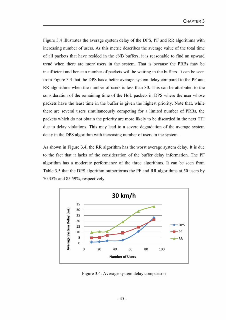
CHAPTER 3
- 45 -
Figure 3.4 illustrates the average system delay of the DPS, PF and RR algorithms with
increasing number of users. As this metric describes the average value of the total time
of all packets that have resided in the eNB buffers, it is reasonable to find an upward
trend when there are more users in the system. That is because the PRBs may be
insufficient and hence a number of packets will be waiting in the buffers. It can be seen
from Figure 3.4 that the DPS has a better average system delay compared to the PF and
RR algorithms when the number of users is less than 80. This can be attributed to the
consideration of the remaining time of the HoL packets in DPS where the user whose
packets have the least time in the buffer is given the highest priority. Note that, while
there are several users simultaneously competing for a limited number of PRBs, the
packets which do not obtain the priority are more likely to be discarded in the next TTI
due to delay violations. This may lead to a severe degradation of the average system
delay in the DPS algorithm with increasing number of users in the system.
As shown in Figure 3.4, the RR algorithm has the worst average system delay. It is due
to the fact that it lacks of the consideration of the buffer delay information. The PF
algorithm has a moderate performance of the three algorithms. It can be seen from
Table 3.5 that the DPS algorithm outperforms the PF and RR algorithms at 50 users by
70.35% and 85.59%, respectively.
Figure 3.4: Average system delay comparison
0
5
10
15
20
25
30
35
0 20 40 60 80 100Ave
rage
Sys
tem
Del
ay (m
s)
Number of Users
30 km/h
DPS
PF
RR
CHAPTER 3
- 46 -
Table 3.5: Average system delay of DPS, PF and RR
10 20 30 50 70 90
DPS 1.00 1.27 2.15 2.76 10.56 22.96
PF 4.84 5.20 7.11 9.31 14.47 21.20
RR 9.88 10.31 10.72 19.15 28.82 33.20
Improvement of DPS
over PF (%)-79.34 -75.58 -69.76 -70.35 -27.02 0.83
Improvement of DPS
over RR (%)-89.88 -87.68 -79.94 -85.59 -63.36 -30.84
Based on the results, it can be concluded that the DPS algorithm is capable of achieving
a better performance in terms of maximizing system throughput and at the same time
minimizing PLR and average system delay. To provide a more attractive overall
performance, the DPS algorithm is suggested in this chapter when compared to the PF
and RR algorithms.
3.3 Summary
A number of single carrier packet scheduling algorithms initially designed in time
domain were discussed in Section 3.1. To compare the performance of these scheduling
algorithms which were developed for different systems under various channel
environments, system level simulations were performed and the results were reported in
Section 3.2 for a downlink LTE system. Adaptations were made to the single carrier
DPS, PF and RR algorithm. The adapted DPS, PF and RR algorithms are referred to as
multi-carrier DPS, PF and RR algorithms respectively. Four performance metrics were
used to evaluate the three algorithms namely system throughput, PLR, fairness and
average system delay. The simulation results showed that the DPS algorithm is able to
provide a better trade-off between maximizing the system performance and
guaranteeing the fairness compared to the PF and RR algorithms.
- 47 -
Chapter 4
QOS AWARE SCHEDULING SCHEMES AND ALGORITHMS
The major difference between mobile cellular systems and fixed line systems is that
resources in mobile cellular systems are bandwidth limited and not always available
because it is shared with other users. Furthermore, inter-cell interference, multipath
fading, shadowing and user mobility cause the unpredictable nature of the wireless radio
path which has an impact on resource allocation. This presents major challenges in
guaranteeing QoS requirements in mobile cellular networks.
In Chapter 3, several time domain packet scheduling algorithms were studied. Due to
the resource allocation structure defined by the LTE standard, frequency domain
scheduling algorithms have been widely investigated for the LTE system. In a multiuser
LTE system, packet scheduling algorithm can benefit by exploiting frequency diversity
and multiuser diversity techniques. The frequency diversity refers to the mechanism
where multiple subcarriers are used simultaneously for transmission to overcome the
effect of frequency-selective fading. The multiuser diversity allows the base station to
select users that experience favourable channel conditions. The diversity techniques
imply that a PRB that is inappropriate for one user may be acceptable for the other users.
It has been shown in [68-71] that frequency domain packet scheduling algorithms can
achieve significantly better performance over conventional time domain only
scheduling algorithms.
This chapter aims at introducing and analyzing frequency domain packet scheduling
algorithms that consider various QoS requirements. A number of scheduling schemes
such as Resource Allocation and Assignment (RAA) scheme, Joint Time and Frequency
Domain Scheduling (JTFDS) scheme and Matrix-Based Scheduling (MBS) scheme are
described and examples of QoS aware packet scheduling algorithms employing these
schemes are presented. To reduce computational complexity of scheduling without
compromising system performance, an efficient Time Domain Grouping Scheduling
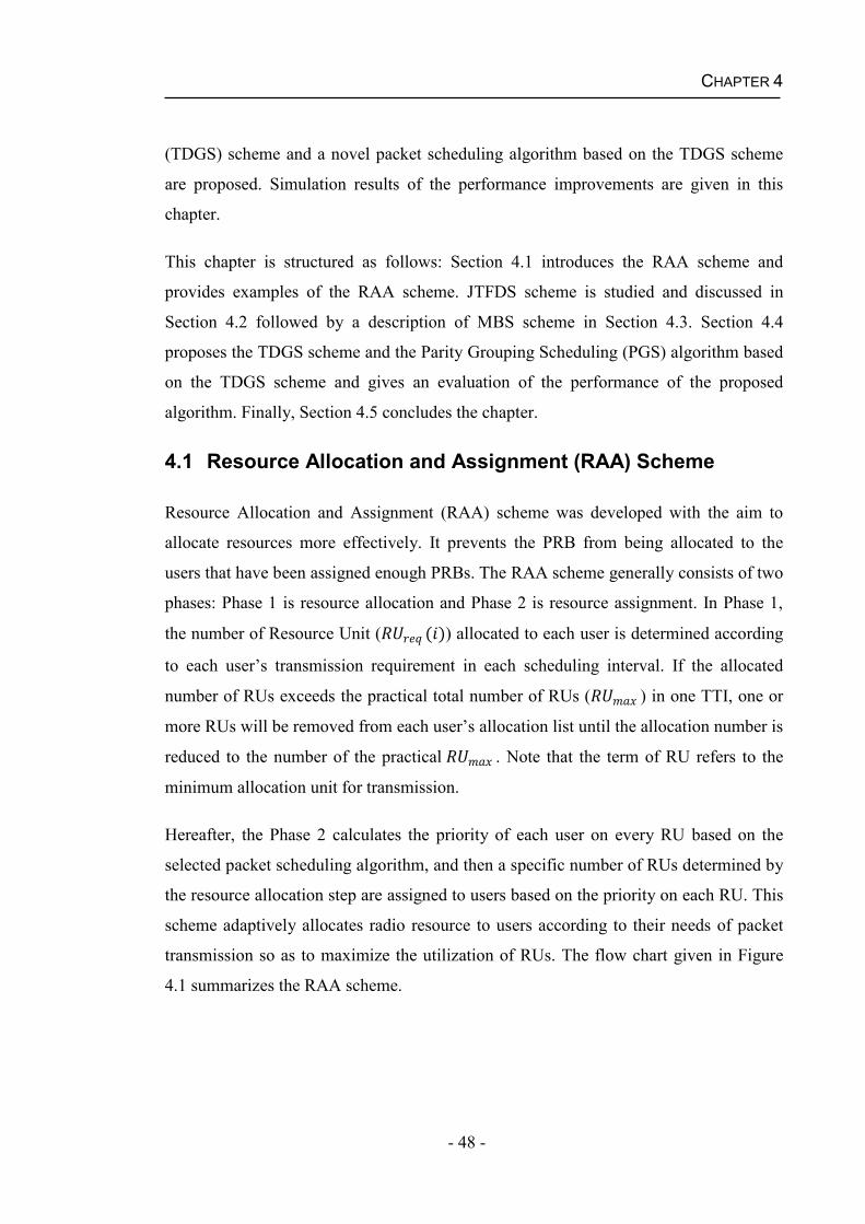
CHAPTER 4
- 48 -
(TDGS) scheme and a novel packet scheduling algorithm based on the TDGS scheme
are proposed. Simulation results of the performance improvements are given in this
chapter.
This chapter is structured as follows: Section 4.1 introduces the RAA scheme and
provides examples of the RAA scheme. JTFDS scheme is studied and discussed in
Section 4.2 followed by a description of MBS scheme in Section 4.3. Section 4.4
proposes the TDGS scheme and the Parity Grouping Scheduling (PGS) algorithm based
on the TDGS scheme and gives an evaluation of the performance of the proposed
algorithm. Finally, Section 4.5 concludes the chapter.
4.1 Resource Allocation and Assignment (RAA) Scheme
Resource Allocation and Assignment (RAA) scheme was developed with the aim to
allocate resources more effectively. It prevents the PRB from being allocated to the
users that have been assigned enough PRBs. The RAA scheme generally consists of two
phases: Phase 1 is resource allocation and Phase 2 is resource assignment. In Phase 1,
the number of Resource Unit ( ( )) allocated to each user is determined according
to each user’s transmission requirement in each scheduling interval. If the allocated
number of RUs exceeds the practical total number of RUs ( ) in one TTI, one or
more RUs will be removed from each user’s allocation list until the allocation number is
reduced to the number of the practical . Note that the term of RU refers to the
minimum allocation unit for transmission.
Hereafter, the Phase 2 calculates the priority of each user on every RU based on the
selected packet scheduling algorithm, and then a specific number of RUs determined by
the resource allocation step are assigned to users based on the priority on each RU. This
scheme adaptively allocates radio resource to users according to their needs of packet
transmission so as to maximize the utilization of RUs. The flow chart given in Figure
4.1 summarizes the RAA scheme.
CHAPTER 4
- 49 -
4.1.1 Load-oriented Scheduling (LOS) Algorithm
To support real time services in OFDMA systems, a frequency domain packet
scheduling algorithm that employs RAA scheme was developed and is referred to as
YES
End
NO
NO
YES
Start
Determine ( )of each user
Sort users on each RU based on a packet scheduling algorithm
Remove one RUfrom the
allocation list of user i ( )
i=i+1
( )=1 > ?
Assign the highest priority user the RUs with the best channel
conditions and remove the assigned RUs from the available RUs list
Have all allocated RUs been assigned to the users?
Choose the next user with
the highest priority
Figure 4.1: Flow chart of the RAA scheme in each TTI
CHAPTER 4
- 50 -
Load-oriented Scheduling (LOS) algorithm [27, 72] throughout this thesis. In each
scheduling interval, the resource allocation phase of LOS contains two steps. In Step 1,
users whose buffers are not empty receive one RU each time in turn while the remaining
RUs are allocated to active users if the list of available RUs is not empty in Step 2. The
total number of RUs that are allocated to user i at TTI t is calculated according to the
following equation:
( ) = ( ) + ( ) ( )==1 + 0.5 (4.1)
where is the number of remaining RUs, ( ) is eNB buffer length (in bits) of
user i at TTI t, and N is the total number of users.
After the resource allocation phase, each user is given a priority in a random fashion
initially in the resource assignment phase. The ( ) RUs are then assigned to user i
with the best channel quality (in terms of CQI) on it based on the priority of user i. In
the next TTI, the priorities of users are exchanged. That is, the user who has the lowest
priority in last TTI will be assigned a highest priority in current TTI. In this way, each
user’s priority is time-varying so as to guarantee a good fairness among the users.
Finally the assigned RUs are removed from the list of the remaining RU. The resource
assignment phase repeats the operation until all the users are given the required number
of RUs determined by the resource allocation step.
4.1.2 Delay First Scheduling (DFS) Algorithm
A packet scheduling algorithm based on M-LWDF algorithm (as studied in Chapter 3)
was designed in [73] to support real time services with different classes of QoS
requirements. This algorithm gives the highest transmission priority to the HoL packet
(as defined in Chapter 2) and is referred to as Delay First Scheduling (DFS) algorithm
throughout this thesis. This algorithm consists of two phases: resource allocation and
resource assignment.
The resource allocation phase determines a fixed number called step-resource-number
based on users’ minimum data rate requirement. Each user is given a constant step-
resource-number of RUs.
CHAPTER 4
- 51 -
The resource assignment in each scheduling interval is divided into four steps. In Step 1,
a RU priority list is created for each user. The RU that has the best channel quality of
will have the highest priority in user i’s RU priority list. In Step 2, the priority of each
user without empty buffer is determined using Equation (4.2).
( ) = ( ) _ ( )( ) ( ) (4.2)
where is the QoS requirement of user i (as defined in Equation (3.8)), ( ) is the
delay of the HoL packet of user i at TTI t. _ ( )is the average data rate on all RUs
of user i at TTI t, ( ) is the average throughput of user i at TTI t (see Equation (3.13)),( ) is the PLR of user i at TTI t and indicates the PLR threshold of user i.
Thereafter, a fixed number of RUs determined from resource allocation phase is given
to each user by priority and the delay of the HoL packets of each user is updated in Step
3. Subsequently, Step 4 computes the HoL delay of users’ transmission packets and
deletes the assigned RUs from the list. Step 2 to Step 4 are repeated until all users’
buffers are empty or all available RUs have been assigned to the users.
4.1.3 Multi-QoS Adaptive Scheduling (MQAS) Algorithm
Different types of traffic have different QoS requirements (see Table 1.2). An algorithm
based on RAA scheme was developed in [74] to allocate radio resource adaptively to a
mixed traffic with different QoS classes. The algorithm is referred to as Multi-QoS
Adaptive Scheduling (MQAS) Algorithm throughout the thesis. A Hebbian learning
process was integrated in this algorithm in order to adapt the scheduling weight
proportion to different kinds of traffic. It was shown that the MQAS algorithm can
guarantee QoS requirements of the real time traffic by reducing the average delay and
packet drop rate and the non real time traffic by balancing the trade-off between
maximizing the system throughput and guaranteeing the fairness.
The resource allocation phase first computes the allocation number of RUs to the real
time traffic. The Hebbian learning process is in charge of calculating and comparing the
change rate of packet drop rate in each scheduling interval and saves this variation
CHAPTER 4
- 52 -
information in a RU Allocation Priority (RAP) vector. If the change rate of packet drop
rate is positive, the weight of the real time traffic is updated using Equation (4.3).
( ) = ( 1) + ( ) > ( 1)( 1) (4.3)
where ( ) is the allocation weight given to the real time users at TTI t and is the
learning rate.
The number of RUs allocated to real time users at scheduling interval t, ( ) can then
be determined based on Equation (4.4).( ) = ( ) ( ( 1) + ( 1)) (4.4)
where ( ) is the total available RUs at TTI t, ( 1) is the proportion of the total
RUs allocated to real time users at TTI t-1 and ( 1) is the allocation weight
given to the real time users at TTI t-1.
Hence, ( ), the RUs allocated to non real time users at scheduling interval t can be
determined using Equation (4.5). ( ) = ( ) ( ) (4.5)
where ( ) is the total available RUs at TTI t and ( ) is the number of RUs
allocated to non real time users at TTI t.
The resource assignment phase performs three steps in each TTI. Step 1 calculates the
priorities of users. Equation (4.6) is used to compute the priority for real time users
while Equation (4.7) gives the priority for non real time users.
( ) = ( ) ( ( ))2 + ( ( ))2 (4.6)
where ( ) is the waiting time of user i from the last scheduled interval until now,
is the buffer delay threshold of real time user i, ( ) is the average channel gain of
RUs for user i at TTI t and ( ) is buffer length of user i at TTI t.
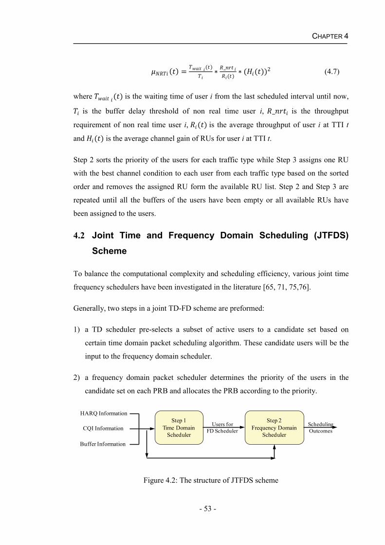
CHAPTER 4
- 53 -
( ) = ( ) _ ( ) ( ( ))2 (4.7)
where ( ) is the waiting time of user i from the last scheduled interval until now,
is the buffer delay threshold of non real time user i, _ is the throughput
requirement of non real time user i, ( ) is the average throughput of user i at TTI t
and ( ) is the average channel gain of RUs for user i at TTI t.
Step 2 sorts the priority of the users for each traffic type while Step 3 assigns one RU
with the best channel condition to each user from each traffic type based on the sorted
order and removes the assigned RU form the available RU list. Step 2 and Step 3 are
repeated until all the buffers of the users have been empty or all available RUs have
been assigned to the users.
4.2 Joint Time and Frequency Domain Scheduling (JTFDS) Scheme
To balance the computational complexity and scheduling efficiency, various joint time
frequency schedulers have been investigated in the literature [65, 71, 75,76].
Generally, two steps in a joint TD-FD scheme are preformed:
1) a TD scheduler pre-selects a subset of active users to a candidate set based on
certain time domain packet scheduling algorithm. These candidate users will be the
input to the frequency domain scheduler.
2) a frequency domain packet scheduler determines the priority of the users in the
candidate set on each PRB and allocates the PRB according to the priority.
Figure 4.2: The structure of JTFDS scheme
Step 1Time Domain
Scheduler
Step 2Frequency Domain
Scheduler
Users for FD Scheduler
Scheduling Outcomes
HARQ Information
CQI Information
Buffer Information
CHAPTER 4
- 54 -
Figure 4.2 shows the structure of the JTFDS scheme. The use of a TD scheduler before
a FD scheduler limits the number of multiplexed users, which helps reduce the
scheduling complexity. Furthermore, it is shown in [71] that the system performance
may achieve its peak when approximately 70% of active users are multiplexed and
degrade when the number of the multiplexed users increases above 70%. Hence,
limiting the number of active users in the FD scheduler contributes to control the system
gain not to exceed its saturation point so as to maximize the system performance.
Moreover, Reference [65, 71] proved that the employment of more than one scheduling
algorithms contributes to a performance improvement. This is mainly because the TD
and FD schedulers with different aims may complement each other.
An algorithm that aims at providing fairness control for real time services based on
JTFDS scheme was proposed in [65]. This algorithm groups users into two sets based
on the channel quality in time domain and employs multiple scheduling policies in one
scheduling interval so as to provide an optimal balance between fairness and cell
throughput. This algorithm is referred to as Oriented Time-Frequency Scheduling
(OTFS) algorithm in this thesis.
In time domain, the OTFS algorithm performs a two-step prioritization and selects a set
of users based on the priorities to share the radio resource in frequency domain. Step 1
separates users into two groups (Group 1 and 2) by a so-called pre-defined Target Bit
Rate (TBR). Users below the TBR from Group 1 are given a higher priority than users
from Group 2. Then, in Step 2, the BET algorithm (as discussed in Section 3.14) is used
to sort users in Group 1 while the PF algorithm (as discussed in Section 3.13) is used in
Group 2. It is worth a mention that if the pre-defined TBR tends to zero then the time
domain scheduling technique is equivalent to the PF algorithm. In this case, the system
throughput is improved as the PF algorithm considers the channel quality of users. On
the contrary, if the predefined TBR tends to infinity then the time domain scheduler
only consists of the BET algorithm which leads to an equal throughput to each user.
Hence, the trade-off between the PF and BET algorithms is controlled by the pre-
defined TBR value.
In frequency domain, a Proportional Fair Scheduled (PFS) algorithm that is an
extension of the PF algorithm was developed to cooperate with the time domain
CHAPTER 4
- 55 -
scheduler. The PFS algorithm gives the highest priority to a user with maximum metric, ( ) in Equation (4.8) at TTI t.
( ) = ( )_ ( ) (4.8)
_ ( + 1) = 1 ( +1)_ _ ( ) + ( +1)_ ( + 1) (4.9)
( + 1) = 1 + 10 + 1(4.10)
where ( ) is the instantaneous data rate (across the whole bandwidth) of user i at TTI t,_ ( ) is the estimated average throughput of user i at TTI t, ( + 1) is a number
(either 0 or 1) indicates if user i is scheduled at TTI t+1 and _ is a time constant
set to 30 [77].
A weight factor is defined in Equation (4.11). The frequency domain scheduler selects a
user with a maximum product of , ( ) by the weight for transmission on PRB j at
TTI t.
= (1, ) (4.11)
where TBR is the target bit rate and ( ) is the average throughput of user i at TTI t.
4.3 Matrix-Based Scheduling (MBS) Scheme
An efficient and effective resource allocation scheme based on channel matrix
calculation is used in some packet scheduling algorithms [78-80]. The Matrix-Based
Scheduling (MBS) scheme is basically divided into two phases: channel matrix
calculation and matrix-based scheduling. The channel matrix calculation forms a
channel matrix that consists of rows representing RUs and columns representing active
users. The element of the channel matrix is the priority of each user on each RU at
scheduling interval t based on certain scheduling algorithm. The channel
matrix is illustrated in Figure 4.3.
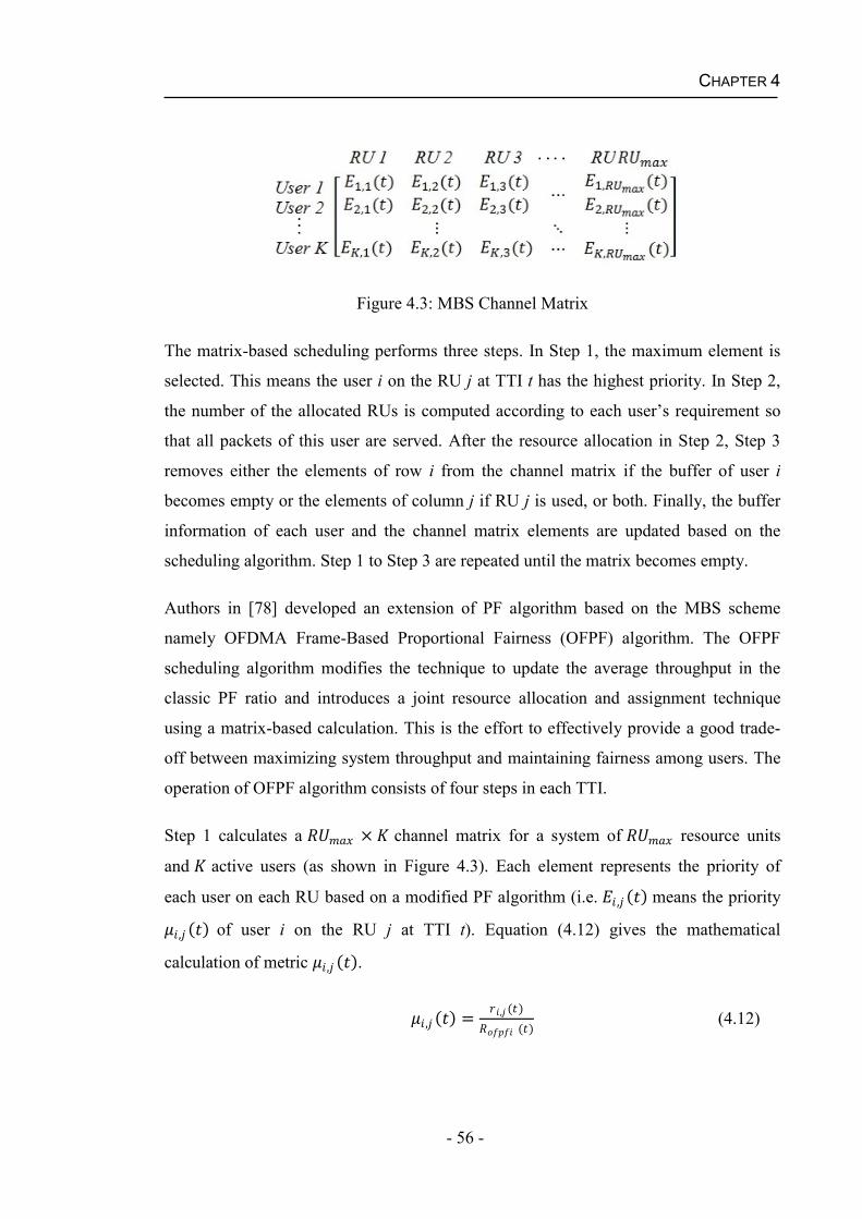
CHAPTER 4
- 56 -
Figure 4.3: MBS Channel Matrix
The matrix-based scheduling performs three steps. In Step 1, the maximum element is
selected. This means the user i on the RU j at TTI t has the highest priority. In Step 2,
the number of the allocated RUs is computed according to each user’s requirement so
that all packets of this user are served. After the resource allocation in Step 2, Step 3
removes either the elements of row i from the channel matrix if the buffer of user i
becomes empty or the elements of column j if RU j is used, or both. Finally, the buffer
information of each user and the channel matrix elements are updated based on the
scheduling algorithm. Step 1 to Step 3 are repeated until the matrix becomes empty.
Authors in [78] developed an extension of PF algorithm based on the MBS scheme
namely OFDMA Frame-Based Proportional Fairness (OFPF) algorithm. The OFPF
scheduling algorithm modifies the technique to update the average throughput in the
classic PF ratio and introduces a joint resource allocation and assignment technique
using a matrix-based calculation. This is the effort to effectively provide a good trade-
off between maximizing system throughput and maintaining fairness among users. The
operation of OFPF algorithm consists of four steps in each TTI.
Step 1 calculates a × channel matrix for a system of resource units
and active users (as shown in Figure 4.3). Each element represents the priority of
each user on each RU based on a modified PF algorithm (i.e. , ( ) means the priority
, ( ) of user i on the RU j at TTI t). Equation (4.12) gives the mathematical
calculation of metric , ( ).
, ( ) = , ( )( ) (4.12)
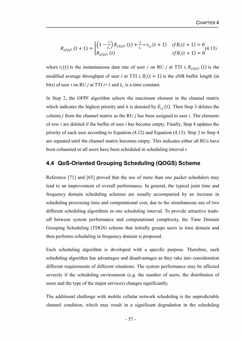
CHAPTER 4
- 57 -
( + 1) = 1 1 ( ) + 1 , ( + 1) ( + 1) > 0( ) ( + 1) = 0(4.13)
where ( ) is the instantaneous data rate of user i on RU j at TTI t, ( ) is the
modified average throughput of user i at TTI t, ( + 1) is the eNB buffer length (in
bits) of user i on RU j at TTI t+1 and is a time constant.
In Step 2, the OFPF algorithm selects the maximum element in the channel matrix
which indicates the highest priority and it is denoted by , ( ). Then Step 3 deletes the
column j from the channel matrix as the RU j has been assigned to user i. The elements
of row i are deleted if the buffer of user i has become empty. Finally, Step 4 updates the
priority of each user according to Equation (4.12) and Equation (4.13). Step 2 to Step 4
are repeated until the channel matrix becomes empty. This indicates either all RUs have
been exhausted or all users have been scheduled in scheduling interval t.
4.4 QoS-Oriented Grouping Scheduling (QOGS) Scheme
Reference [71] and [65] proved that the use of more than one packet schedulers may
lead to an improvement of overall performance. In general, the typical joint time and
frequency domain scheduling schemes are usually accompanied by an increase in
scheduling processing time and computational cost, due to the simultaneous use of two
different scheduling algorithms in one scheduling interval. To provide attractive trade-
off between system performance and computational complexity, the Time Domain
Grouping Scheduling (TDGS) scheme that initially groups users in time domain and
then performs scheduling in frequency domain is proposed.
Each scheduling algorithm is developed with a specific purpose. Therefore, each
scheduling algorithm has advantages and disadvantages as they take into consideration
different requirements of different situations. The system performance may be affected
severely if the scheduling environment (e.g. the number of users, the distribution of
users and the type of the major services) changes significantly.
The additional challenge with mobile cellular network scheduling is the unpredictable
channel condition, which may result in a significant degradation in the scheduling
CHAPTER 4
- 58 -
performance when a single scheduling algorithm under certain condition is used. These
problems can be alleviated by the QOGS scheme that adaptively and intelligently
selects from a group of scheduling algorithms instead of a single packet scheduling
algorithm in an interval of time so as to be more tolerant to the inconsistent mobile
environment.
The QOGS scheme separates the whole simulation interval into several groups. For
example, Group 1 contains all resource blocks for TTI 1, TTI 2, and TTI 3. Each group
consists of a fixed number of TTIs (l is used to denote the length of the TTI group) and
each TTI of the group employs a single scheduling algorithm. Note that the scheduling
algorithm used in each TTI of the group can either be identical or different from the
others. In order to achieve the best scheduling performance, the length of the TTI group
and the combination of the scheduling algorithms can be configured based on the QoS
requirements of the traffics.
Figure 4.4:An illustration of the QOGS scheme
CHAPTER 4
- 59 -
Assuming a system mainly consists of GBR services which are more sensitive to packet
delay rather than packet loss ratio. A reasonable configuration of the group length could
be l=3 and the group of scheduling algorithms could be the combination of the M-
LWDF, DPS and PF algorithms. Figure 4.4 gives an illustration of the QOGS scheme
based on this configuration.
4.4.1 Parity Grouping Scheduling (PGS) Algorithm
Based on the TDGS scheme, an algorithm referred to as Parity Grouping Scheduling
(PGS) algorithm is proposed in this section. The PGS algorithm employs two well-
known packet scheduling algorithms: modified multi-carrier Max-Rate algorithm (as
described in Section 3.2.1) and modified multi-carrier M-LWDF algorithm with the aim
to maximize the overall system performance without compromising the QoS
requirements. The multi-carrier Max-Rate and M-LWDF algorithms are modified from
the single-carrier Max-Rate and M-LWDF algorithms to adapt to multi-subcarrier LTE
system (for simplicity, they are referred to as Max-Rate and M-LWDF algorithms
hereinafter). The M-LWDF algorithm schedules a user with maximum metric , ( ) in
Equation (4.14) for transmission on PRB j at TTI t.
, ( ) = ( ) , ( )( ) (4.14)
= ( ) (4.15)
where , ( ) is the priority of user i on PRB j at TTI t, is the QoS requirement of
user i, ( ) is the delay of the HoL packet of user i at TTI t, , ( ) is the instantaneous
data rate of user i on PRB j at TTI t, ( ) is the average throughput of user i at TTI t,
indicates the PLR threshold of user i and is the buffer delay threshold of user i.
The Max-Rate algorithm is expected to be effective to achieve an excellent system
throughput performance due to the fact that it always gives the highest scheduling
priority to the user who is experiencing the best channel condition. Compared with the
Max-Rate algorithm, the M-LWDF algorithm is more likely to provide comprehensive
and satisfactory QoS for real time services as it has an overall consideration of packet
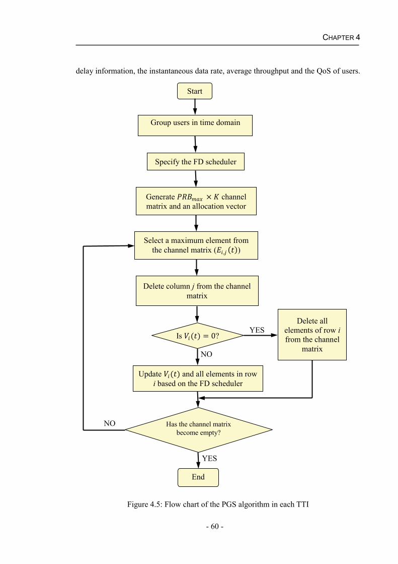
CHAPTER 4
- 60 -
delay information, the instantaneous data rate, average throughput and the QoS of users.
Figure 4.5: Flow chart of the PGS algorithm in each TTI
YES
NO
YES
NO
Delete all elements of row ifrom the channel
matrix
End
Has the channel matrix become empty?
Update ( ) and all elements in row i based on the FD scheduler
Start
Group users in time domain
Specify the FD scheduler
Generate × channel matrix and an allocation vector
Select a maximum element from the channel matrix ( , ( ))
Delete column j from the channel matrix
Is ( ) = 0?
CHAPTER 4
- 61 -
The PGS algorithm performs three steps in each scheduling interval. Figure 4.5 shows
the flow chart of the PGS algorithm. Detailed description of each step is given below.
Step1
At TTI t, if t is an odd number, then the M-LWDF algorithm is selected as the FD
scheduler, otherwise, the Max-Rate algorithm is selected as the FD scheduler. The
employment of more than one scheduling algorithms with different aims in two adjacent
TTIs alternately complement each other in long-term and the computational cost will
not increase as only one single scheduling algorithm is applied in each TTI.
Step 2
The priority of each user on each PRB according to the specified FD scheduling
algorithm (i.e. the Max-Rate or the M-LWDF algorithm) is calculated and a ×channel matrix consisting of PRBs and active users (see Figure 4.3) is
generated. Each element of the channel matrix is the priority of each user on each PRB.
In the mean time, the number of PRBs required by each user is calculated and the
information is stored in an allocation vector ( ( )).
Step 3
Step 3 iterates over all the elements in the channel matrix and selects the maximum
element ( , ( )). This means user i has the highest priority on PRB j and system
performance will be maximized by assigning PRB j to user i. Subsequently, all the
elements of column j are deleted and row i is removed from the channel matrix if the
required number of PRBs have been assigned to user i according to the allocation vector.
Then, elements in the channel matrix are updated based on the specified FD scheduling
algorithm and the allocation vector is updated based on the buffer information of each
user. Step 3 is repeated until all the users have been assigned required number of PRBs
or all the remaining available PRBs have been assigned to the users.
4.4.2 Performance of the PGS algorithm for real time services
The performance of the proposed PGS algorithm is evaluated in this section. The
system throughput, PLR, average system queuing delay and fairness were used to
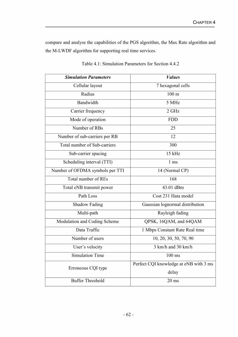
CHAPTER 4
- 62 -
compare and analyse the capabilities of the PGS algorithm, the Max Rate algorithm and
the M-LWDF algorithm for supporting real time services.
Table 4.1: Simulation Parameters for Section 4.4.2
Simulation Parameters Values
Cellular layout 7 hexagonal cells
Radius 100 m
Bandwidth 5 MHz
Carrier frequency 2 GHz
Mode of operation FDD
Number of RBs 25
Number of sub-carriers per RB 12
Total number of Sub-carriers 300
Sub-carrier spacing 15 kHz
Scheduling interval (TTI) 1 ms
Number of OFDMA symbols per TTI 14 (Normal CP)
Total number of REs 168
Total eNB transmit power 43.01 dBm
Path Loss Cost 231 Hata model
Shadow Fading Gaussian lognormal distribution
Multi-path Rayleigh fading
Modulation and Coding Scheme QPSK, 16QAM, and 64QAM
Data Traffic 1 Mbps Constant Rate Real time
Number of users 10, 20, 30, 50, 70, 90
User’s velocity 3 km/h and 30 km/h
Simulation Time 100 ms
Erroneous CQI typePerfect CQI knowledge at eNB with 3 ms
delay
Buffer Threshold 20 ms
CHAPTER 4
- 63 -
The downlink LTE system model described in Section 2.1 was considered and the
detailed simulation assumptions that were previously summarized in Section 2.2 and
Section 2.3 were used. Besides the above assumptions, this section made some
additional simulation settings: (i) the eNB has a perfect knowledge of CQIs reported
from the users, (ii) due to the practical transmission and processing delay, a 3 ms CQI
feedback delay was considered at the eNB, (iii) the buffer delay thresholds of the real
time services is set to 20ms [81].
Based on the 3GPP Technical Spec 23.203 [26], the GBR PLR threshold was set to 10 2 while the threshold of the GBR average system buffer delay was capped at 80 ms.
These parameter settings aim to optimize the system performance for GBR services and
limit the discussion of the performance evaluation within an effective range. To
compare the QoS of GBR services under various speed scenarios, user velocity was set
to 3 km/h and 30 km/h respectively. The detailed simulation parameters are listed in
Table 4.1.
The system throughput of seven cells of the PGS, Max-Rate and M-LWDF algorithms
with increasing number of users at 3 km/h and 30 km/h are compared in Figure 4.6 and
Figure 4.7, respectively. It can be seen from Figure 4.6 and Figure 4.7 that the Max-
Rate algorithm has the best throughput as expected because the algorithm always gives
the highest scheduling priority to users who have the best channel quality. In
comparison, the M-LWDF algorithm has the worst throughput performance. This is
because, besides the instantaneous channel quality, it takes into account more factors
such as the average throughput and the delay of the HoL packets of the user. Thereafter,
the M-LWDF algorithm outperforms the Max-Rate algorithm in terms of other aspects,
such as fairness and PLR. This can be justified next.
Moreover, it can be seen from Figure 4.6 and Figure 4.7 that with increasing user
velocity, the overall system throughput of the three algorithms degrades. This can be
explained that the system gains reduce with the poor BLER and the erroneous user’s
throughput estimation [82, 83], and because of the 3 ms CQI delay, the difference
between the instantaneous CQI that experienced by a user and the current CQI that
received by the scheduler (i.e. the eNB) becomes larger at a higher user velocity, hence,
the corresponding MCS may be computed incorrectly. These chain problems caused by
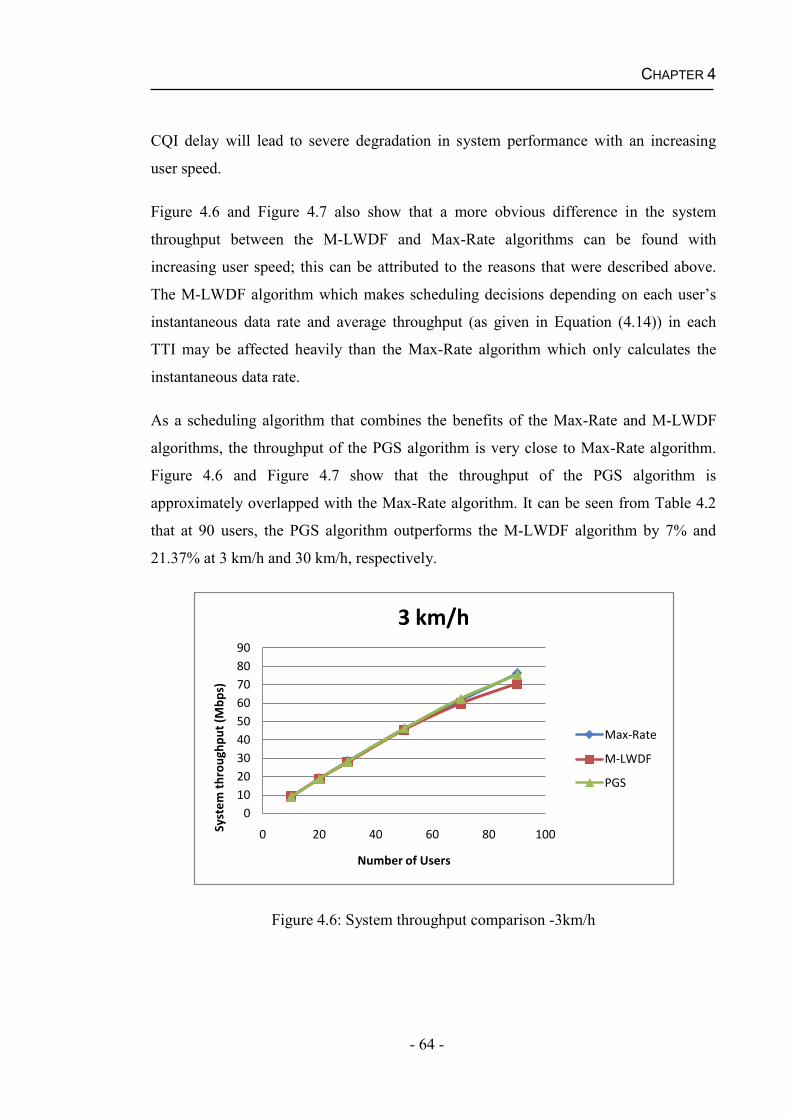
CHAPTER 4
- 64 -
CQI delay will lead to severe degradation in system performance with an increasing
user speed.
Figure 4.6 and Figure 4.7 also show that a more obvious difference in the system
throughput between the M-LWDF and Max-Rate algorithms can be found with
increasing user speed; this can be attributed to the reasons that were described above.
The M-LWDF algorithm which makes scheduling decisions depending on each user’s
instantaneous data rate and average throughput (as given in Equation (4.14)) in each
TTI may be affected heavily than the Max-Rate algorithm which only calculates the
instantaneous data rate.
As a scheduling algorithm that combines the benefits of the Max-Rate and M-LWDF
algorithms, the throughput of the PGS algorithm is very close to Max-Rate algorithm.
Figure 4.6 and Figure 4.7 show that the throughput of the PGS algorithm is
approximately overlapped with the Max-Rate algorithm. It can be seen from Table 4.2
that at 90 users, the PGS algorithm outperforms the M-LWDF algorithm by 7% and
21.37% at 3 km/h and 30 km/h, respectively.
Figure 4.6: System throughput comparison -3km/h
0102030405060708090
0 20 40 60 80 100Syst
em t
hrou
ghpu
t (M
bps)
Number of Users
3 km/h
Max-Rate
M-LWDF
PGS
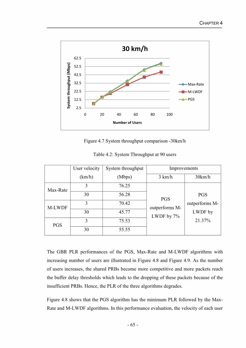
CHAPTER 4
- 65 -
Figure 4.7 System throughput comparison -30km/h
Table 4.2: System Throughput at 90 users
User velocity
(km/h)
System throughput
(Mbps)
Improvements
3 km/h 30km/h
Max-Rate3 76.25
PGS
outperforms M-
LWDF by 7%
PGS
outperforms M-
LWDF by
21.37%
30 56.28
M-LWDF3 70.42
30 45.77
PGS3 75.53
30 55.55
The GBR PLR performances of the PGS, Max-Rate and M-LWDF algorithms with
increasing number of users are illustrated in Figure 4.8 and Figure 4.9. As the number
of users increases, the shared PRBs become more competitive and more packets reach
the buffer delay thresholds which leads to the dropping of these packets because of the
insufficient PRBs. Hence, the PLR of the three algorithms degrades.
Figure 4.8 shows that the PGS algorithm has the minimum PLR followed by the Max-
Rate and M-LWDF algorithms. In this performance evaluation, the velocity of each user
2.5
12.5
22.5
32.5
42.5
52.5
62.5
0 20 40 60 80 100
Syst
em t
hrou
ghpu
t (M
bps)
Number of Users
30 km/h
Max-Rate
M-LWDF
PGS
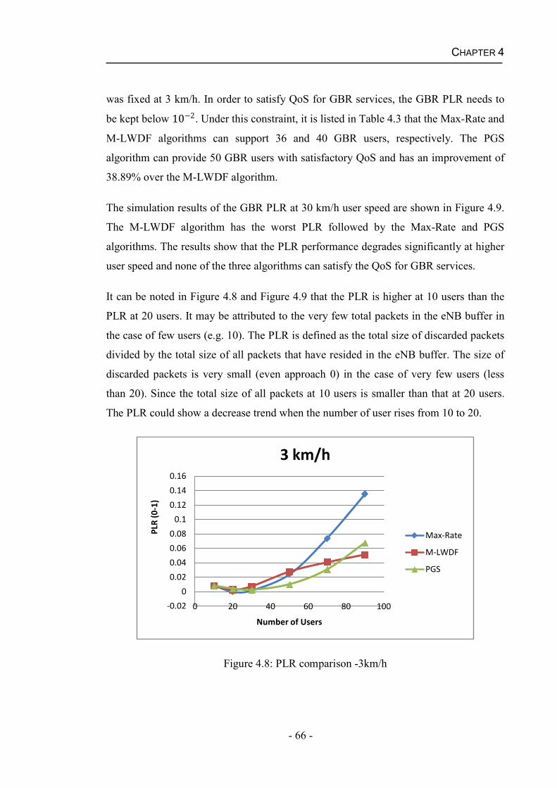
CHAPTER 4
- 66 -
was fixed at 3 km/h. In order to satisfy QoS for GBR services, the GBR PLR needs to
be kept below 10 2. Under this constraint, it is listed in Table 4.3 that the Max-Rate and
M-LWDF algorithms can support 36 and 40 GBR users, respectively. The PGS
algorithm can provide 50 GBR users with satisfactory QoS and has an improvement of
38.89% over the M-LWDF algorithm.
The simulation results of the GBR PLR at 30 km/h user speed are shown in Figure 4.9.
The M-LWDF algorithm has the worst PLR followed by the Max-Rate and PGS
algorithms. The results show that the PLR performance degrades significantly at higher
user speed and none of the three algorithms can satisfy the QoS for GBR services.
It can be noted in Figure 4.8 and Figure 4.9 that the PLR is higher at 10 users than the
PLR at 20 users. It may be attributed to the very few total packets in the eNB buffer in
the case of few users (e.g. 10). The PLR is defined as the total size of discarded packets
divided by the total size of all packets that have resided in the eNB buffer. The size of
discarded packets is very small (even approach 0) in the case of very few users (less
than 20). Since the total size of all packets at 10 users is smaller than that at 20 users.
The PLR could show a decrease trend when the number of user rises from 10 to 20.
Figure 4.8: PLR comparison -3km/h
-0.02
0
0.02
0.04
0.06
0.08
0.1
0.12
0.14
0.16
0 20 40 60 80 100
PLR
(0-1
)
Number of Users
3 km/h
Max-Rate
M-LWDF
PGS
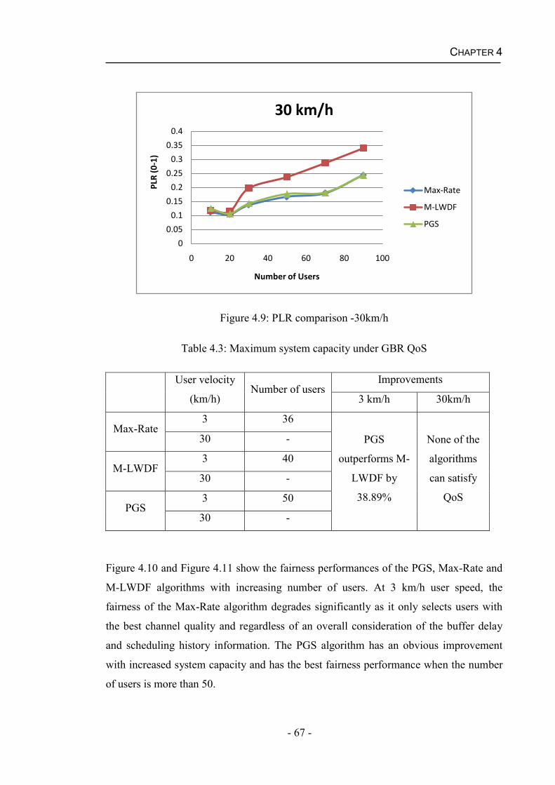
CHAPTER 4
- 67 -
Figure 4.9: PLR comparison -30km/h
Table 4.3: Maximum system capacity under GBR QoS
User velocity
(km/h)Number of users
Improvements
3 km/h 30km/h
Max-Rate3 36
PGS
outperforms M-
LWDF by
38.89%
None of the
algorithms
can satisfy
QoS
30 -
M-LWDF3 40
30 -
PGS3 50
30 -
Figure 4.10 and Figure 4.11 show the fairness performances of the PGS, Max-Rate and
M-LWDF algorithms with increasing number of users. At 3 km/h user speed, the
fairness of the Max-Rate algorithm degrades significantly as it only selects users with
the best channel quality and regardless of an overall consideration of the buffer delay
and scheduling history information. The PGS algorithm has an obvious improvement
with increased system capacity and has the best fairness performance when the number
of users is more than 50.
0
0.05
0.1
0.15
0.2
0.25
0.3
0.35
0.4
0 20 40 60 80 100
PLR
(0-1
)
Number of Users
30 km/h
Max-Rate
M-LWDF
PGS
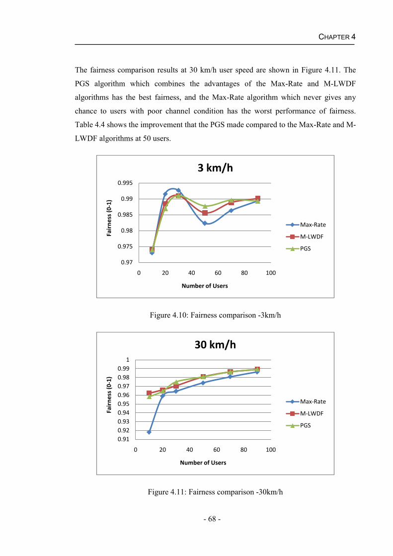
CHAPTER 4
- 68 -
The fairness comparison results at 30 km/h user speed are shown in Figure 4.11. The
PGS algorithm which combines the advantages of the Max-Rate and M-LWDF
algorithms has the best fairness, and the Max-Rate algorithm which never gives any
chance to users with poor channel condition has the worst performance of fairness.
Table 4.4 shows the improvement that the PGS made compared to the Max-Rate and M-
LWDF algorithms at 50 users.
Figure 4.10: Fairness comparison -3km/h
Figure 4.11: Fairness comparison -30km/h
0.97
0.975
0.98
0.985
0.99
0.995
0 20 40 60 80 100
Fair
ness
(0-1
)
Number of Users
3 km/h
Max-Rate
M-LWDF
PGS
0.910.920.930.940.950.960.970.980.99
1
0 20 40 60 80 100
Fair
ness
(0-1
)
Number of Users
30 km/h
Max-Rate
M-LWDF
PGS
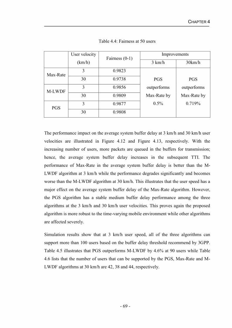
CHAPTER 4
- 69 -
Table 4.4: Fairness at 50 users
User velocity
(km/h)Fairness (0-1)
Improvements
3 km/h 30km/h
Max-Rate3 0.9823
PGS
outperforms
Max-Rate by
0.5%
PGS
outperforms
Max-Rate by
0.719%
30 0.9738
M-LWDF3 0.9856
30 0.9809
PGS3 0.9877
30 0.9808
The performance impact on the average system buffer delay at 3 km/h and 30 km/h user
velocities are illustrated in Figure 4.12 and Figure 4.13, respectively. With the
increasing number of users, more packets are queued in the buffers for transmission;
hence, the average system buffer delay increases in the subsequent TTI. The
performance of Max-Rate in the average system buffer delay is better than the M-
LWDF algorithm at 3 km/h while the performance degrades significantly and becomes
worse than the M-LWDF algorithm at 30 km/h. This illustrates that the user speed has a
major effect on the average system buffer delay of the Max-Rate algorithm. However,
the PGS algorithm has a stable medium buffer delay performance among the three
algorithms at the 3 km/h and 30 km/h user velocities. This proves again the proposed
algorithm is more robust to the time-varying mobile environment while other algorithms
are affected severely.
Simulation results show that at 3 km/h user speed, all of the three algorithms can
support more than 100 users based on the buffer delay threshold recommend by 3GPP.
Table 4.5 illustrates that PGS outperforms M-LWDF by 4.6% at 90 users while Table
4.6 lists that the number of users that can be supported by the PGS, Max-Rate and M-
LWDF algorithms at 30 km/h are 42, 38 and 44, respectively.
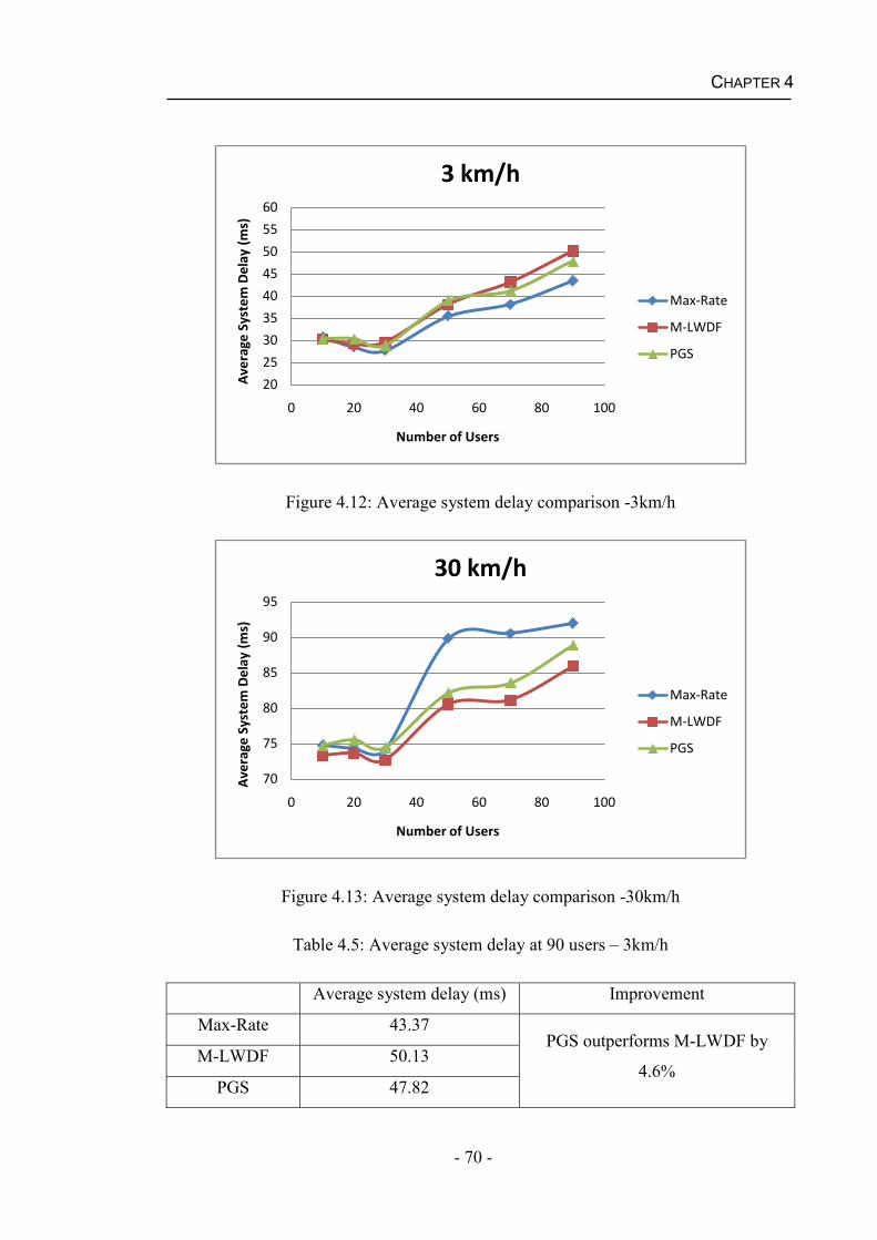
CHAPTER 4
- 70 -
Figure 4.12: Average system delay comparison -3km/h
Figure 4.13: Average system delay comparison -30km/h
Table 4.5: Average system delay at 90 users – 3km/h
Average system delay (ms) Improvement
Max-Rate 43.37PGS outperforms M-LWDF by
4.6%M-LWDF 50.13
PGS 47.82
20
25
30
35
40
45
50
55
60
0 20 40 60 80 100
Ave
rage
Sys
tem
Del
ay (m
s)
Number of Users
3 km/h
Max-Rate
M-LWDF
PGS
70
75
80
85
90
95
0 20 40 60 80 100
Ave
rage
Sys
tem
Del
ay (m
s)
Number of Users
30 km/h
Max-Rate
M-LWDF
PGS
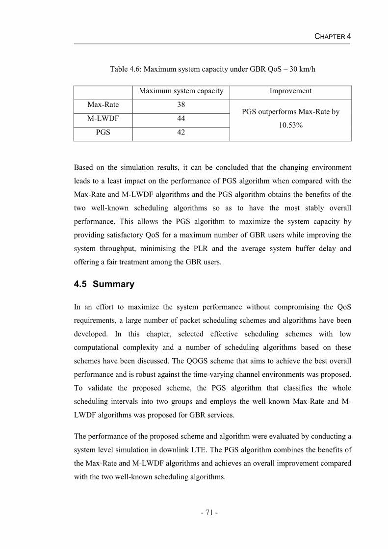
CHAPTER 4
- 71 -
Table 4.6: Maximum system capacity under GBR QoS – 30 km/h
Maximum system capacity Improvement
Max-Rate 38PGS outperforms Max-Rate by
10.53%M-LWDF 44
PGS 42
Based on the simulation results, it can be concluded that the changing environment
leads to a least impact on the performance of PGS algorithm when compared with the
Max-Rate and M-LWDF algorithms and the PGS algorithm obtains the benefits of the
two well-known scheduling algorithms so as to have the most stably overall
performance. This allows the PGS algorithm to maximize the system capacity by
providing satisfactory QoS for a maximum number of GBR users while improving the
system throughput, minimising the PLR and the average system buffer delay and
offering a fair treatment among the GBR users.
4.5 Summary
In an effort to maximize the system performance without compromising the QoS
requirements, a large number of packet scheduling schemes and algorithms have been
developed. In this chapter, selected effective scheduling schemes with low
computational complexity and a number of scheduling algorithms based on these
schemes have been discussed. The QOGS scheme that aims to achieve the best overall
performance and is robust against the time-varying channel environments was proposed.
To validate the proposed scheme, the PGS algorithm that classifies the whole
scheduling intervals into two groups and employs the well-known Max-Rate and M-
LWDF algorithms was proposed for GBR services.
The performance of the proposed scheme and algorithm were evaluated by conducting a
system level simulation in downlink LTE. The PGS algorithm combines the benefits of
the Max-Rate and M-LWDF algorithms and achieves an overall improvement compared
with the two well-known scheduling algorithms.
CHAPTER 4
- 72 -
A number of metrics were used to compare and analyse the proposed algorithm and the
reference algorithms, such as system throughput, PLR, fairness and system buffer delay.
The simulation results show that the proposed algorithm maintains a good and stable
scheduling capacity while the performances of the Max-Rate and M-LWDF algorithms
degrade significantly due to the change of user mobility and the delay of the CQI
feedback.
Various imperfect CQI situations and an erroneous knowledge of CQI at eNB should be
considered in a more practical mobile cellular system. Packet scheduling with the
imperfect CQI is discussed and addressed in the next chapter.
- 73 -
Chapter 5
PACKET SCHEDULING WITH IMPERFECT CQI
Channel-dependent scheduling of users’ data packets in a wireless system is based on
measurement and feedback of the channel quality. The feedback and processing delay
cause a mismatch between the current channel state and the CQI received by the
scheduler [84], along with the interference, multi-path fading, and shadowing due to the
unpredictable nature of wireless channel. Therefore it is highly unlikely to have a
perfect CQI report at the scheduler end in a practical downlink LTE system. System
performance may degrade significantly for employing a channel-dependent packet
scheduler that has continuously received inaccurate CQI reports.
Practical channel conditions where the CQI feedback experiences delay or the CQI is
unavailable (when the delay of the outdated CQI is longer than the scheduling interval,
CQI is unavailable) are considered in this chapter. To alleviate the performance
degradation due to outdated and unavailable CQI, a novel packet scheduling algorithm
referred to as Channel Predictive Grouping Scheduling (CPGS) algorithm is proposed in
this chapter for the real time traffic in downlink LTE system. A frequency domain
channel predictor based on Kalman filter is initially developed to recover the correct
CQI from erroneous channel quality feedback. Then the PGS algorithm (as discussed in
Section 4.4.1) based on a time domain grouping scheme makes the scheduling decision
according to the estimated CQI. It was proved by simulation results that this proposed
scheduling algorithm achieves a better overall performance under imperfect channel
conditions compared to a conventional scheduling algorithm.
This chapter is organized as follows: Section 5.1 studies a number of packet scheduling
algorithms which were designed for the imperfect channel quality. Section 5.2 provides
a thorough discussion of the Least Squares (LS) estimation and the Kalman filter. A
detailed description of the CPGS algorithm is given in Section 5.3 followed by the
CHAPTER 5
- 74 -
performance evaluation of the Kalman filter based channel predictor and the CPGS
algorithm in Section 5.4. Finally, Section 5.5 summaries this chapter.
5.1 Packet Scheduling Algorithms under Practical Channel Condition
To overcome the detrimental effects due to imperfect channel condition, a number of
scheduling algorithms were developed with effective techniques, such as HARQ or
channel prediction. This section introduces scheduling algorithms designed for
imperfect CQI reports.
5.1.1 HARQ Aware Scheduling (HAS) Algorithm
HARQ technique is a combination of Forward Error Correction (FEC) and Automatic
Repeat Request (ARQ) [53]. Since the HARQ technique can improve efficiency of
decoding and transmission by combining multiple retransmissions, a number of packet
scheduling algorithms based on HARQ technique were developed. One of these
algorithms is referred to as HARQ Aware Scheduling (HAS) algorithm [85]. This
algorithm assumes error-prone wireless channels in the downlink LTE system with a
high probability to incorrectly decode received packets at the UE end.
HAS algorithm extends the well-known M-LWDF algorithm to provide satisfactory
QoS for GBR services which have a stricter requirement on packet delay compared to
Non-GBR services. To minimize PLR and average system delay, retransmission users
are given a higher scheduling priority as packets of these HARQ users are more likely
to approach their buffer delay threshold. The HAS algorithm schedules a user with
maximum metric , ( ) in Equation (5.1) for transmission on PRB j at TTI t.
, ( ) = ( ) , ( )( ) & ( ) , ( )( ) ( )( ) & ( ) < , ( )( ) , ( )( ) (5.1)
where , ( ) is the priority of user i on PRB j at TTI t, is the QoS requirement of
user i (as defined in Equation (3.9)), ( ) is the delay of the HoL packet of user i at
CHAPTER 5
- 75 -
TTI t, ( ) is the eNB buffer length (in bits) of user i at TTI t, , ( ) is the
instantaneous data rate of user i on PRB j at TTI t, ( ) is the average throughput of
user i at TTI t, is the buffer delay threshold of user i and is a constant parameter.
5.1.2 Robust and QoS-Driven Scheduling (RQ-DS) Algorithm
An algorithm known as Robust and QoS-Driven Scheduling (RQ-DS) algorithm based
on the HARQ scheme was developed in [86]. This algorithm employs an extension of
the well-known M-LWDF algorithm to support QoS for real time services. The RQ-DS
algorithm consists of four steps in each scheduling interval. Step 1 and Step 2 are in
charge of resource allocation while Step 3 and Step 4 conduct the resource assignment.
In Step 1, it determines the packet size to be retransmitted of each pending HARQ user
and calculates the total number of PRBs required by HARQ users. This is the effort to
guarantee a sufficient amount of PRBs allocated to each retransmission user.
If the number of the allocated PRBs ( ) exceeds the total number of PRBs
( ) in one TTI after the resource allocation in Step 1, then Step 2 is executed. To
remove the over-assigned PRBs from the allocation list, Step 2 reduces the number of
allocated PRBs on the basis of users. Each HARQ user is given a random priority and
sorted in ascending order. Step 2 deletes a HARQ user in turn until the number of the
allocated PRBs is no more than the total number of PRBs ( <= ).
Step 3 is performed if < after the implementation of previous steps.
Step 3 is in charge of the resource assignment to new users and divided into channel
matrix calculation and matrix-based scheduling. The channel matrix calculation forms a
matrix that consists of new users and PRBs (see Figure 4.3). The element
of the channel matrix is the priority of each user on each PRB at scheduling interval t
based on the multi-carrier M-LWDF algorithm (as defined in Equation (4.14)).
The matrix-based scheduling initially selects an maximum element (e.g. , ( )). This
indicates the user i on the PRB j at TTI t has the highest priority according to the M-
LWDF algorithm. After assigning PRB j to user i, it deletes all the elements of column j
and removes row i from the channel matrix if the buffer of user i becomes empty.
CHAPTER 5
- 76 -
Subsequently, elements in the channel matrix are updated using Equation (4.14). This
process is repeated until all the remaining available PRBs (i.e. , =) have been assigned to the new users.
Due to the fact that retransmission packets are more likely to be received correctly, the
resource assignment for HARQ users in Step 4 is executed after the resource assignment
for new users in Step 3 if > 0. Unlike Step 3, it sorts the allocated HARQ
users in a random order and assigns the required number of PRBs to the allocated
HARQ users. Step 4 is repeated until all the have been assigned.
5.1.3 HARQ Aware TD-FD Scheduling (HATFS) Algorithm
To provide a trade-off between throughput and coverage while maintaining a fair
treatment among users, the authors in [76] proposed a joint TD and FD packet
scheduling algorithm with HARQ technique. This algorithm is referred to as HARQ
Aware TD-FD Scheduling (HATFS) algorithm in this thesis. A time domain BET
algorithm (as described in Section 3.1.4) is used in each scheduling interval to select a
set of users (both new users and retransmission users) that have the least average
throughput (through the whole simulation interval) in the past. Note that the
retransmission users are not prioritized over new users by the BET scheduler.
A frequency domain scheduling algorithm called Throughput-to-Average (TTA) [87]
algorithm is employed as the frequency scheduler. This algorithm balances throughput
and fairness by using a normalization factor ( , ( )( ) ) of the instantaneous throughput on
the specified PRB. Similar to the PF algorithm, it prefers a user that has a lower overall
expected throughput. The TTA algorithm schedules a user with maximum metric , ( )in Equation (5.2) for transmission on PRB j at TTI t.
, ( ) = , ( )( ) (5.2)
where , ( ) is the priority of user i on PRB j at TTI t, , ( ) is the instantaneous data
rate of user i on PRB j at TTI t, ( )is the instantaneous data rate (across the whole
bandwidth) of user i at TTI t.
CHAPTER 5
- 77 -
The FD scheduler performs three steps in each scheduling interval. Step 1 determines
the number of PRBs allocated to retransmission and new users, respectively. To ensure
a sufficient number of PRBs for HARQ users, they are allocated PRBs prior to new
users. Hence, the remaining PRBs are assigned to the first time transmission users.
After the determination of the allocated PRBs, a required number of PRBs are assigned
to users with relative good channel quality on it according to the TTA algorithm in Step
2. As it is more likely to successfully decode retransmission packets due to the fact that
retransmission data have a greater chance to be decoded correctly at the receiver
compared to new users, the assignment of PRBs to HARQ users takes place after that of
the new users.
5.1.4 Advanced Proportionally Fair Scheduling (APFS) Algorithm
In order to dynamically adapt to the imperfect CQI in time-varying channel, a
scheduling algorithm based on enhancement HARQ technique was developed for TDD-
CDMA which supports High Speed Downlink Packet Access (HSDPA) techniques [88].
This algorithm is called Advanced Proportionally Fair Scheduling (APFS) algorithm in
this thesis. The basic idea of enhancement HARQ is to terminate the retransmission and
change the modulation and coding (MAC) when the CQI is lower than a pre-defined
threshold. It was defined in the APFS algorithm that the MCS for retransmission is the
same as the original transmission. In each scheduling interval, the APFS algorithm
selects a user that maximizes metric ( ) in the following equation:
( ) = ( ) ( )==1 ( ) ( )( ) (5.3)
( ) = ( 1) + (1 ) ( 1) (5.4)
where ( ) is the priority of user i at scheduling interval t, ( ) is the average
throughput required by user i at TTI t and ( ) is the instantaneous data rate (across the
whole bandwidth) of user i at TTI t. Moreover, ( ) represents the average data rate
over a number of scheduling intervals of user i at TTI t (updated using Equation (5.4))
and ( ) is the average throughput of user i at scheduling interval t (see Equation (3.3)).
In addition, is a constant parameter and N is the total number of users.
CHAPTER 5
- 78 -
5.2 Channel Prediction
The scheduling algorithms discussed in Section 5.1 take practical channel conditions
into account and allows an erroneous CQI or delayed CQI situation in their simulations.
However, the CQI report is assumed to be available at the scheduler for the scheduling
algorithms. When the delay of an outdated CQI is more than the scheduling interval, it
becomes unavailable and the system performance degrades further when the scheduler
misses the CQI reports in a number of consecutive scheduling intervals [29]. To
effectively address problems caused by unavailable CQIs, the combination of channel
prediction and resource allocation has been widely investigated [29, 64, 68, 84, 89, 90].
This section gives detailed descriptions of the well-known least squares estimation and
Kalman Filter in Sections 5.2.1 and 5.2.2, respectively.
5.2.1 Least Squares Estimation
The method of least squares is the most widely used estimation approach especially for
over-determined systems where the state equations are more than unknown states [91].
The overall objective of the least squares method is to minimize the sum of the squares
of the errors made in each estimation.
Assume there is a fixed, but unknown state . ( ) is a sequence of observation
values that can be described in the following way:( ) = + (5.9)
where is the system gain and is the additive noise. Without the loss of generality,
no explicit assumption is made about the additive noise .
The difference between the estimation of and itself indicates the estimation error
of and it can be mathematically expressed using Equation (5.10).( ) = ( ) (5.10)
where is the current state, is the estimation of and is the estimation error
between and .
CHAPTER 5
- 79 -
To estimate the unknown state through the k observations in the value of , the
approximate solution of least squares method is to minimize the estimation error .
Equation (5.11) gives the mathematical expression for the estimation error.( ) = ( )2 (5.11)
5.2.2 Kalman Filter
In 1960, Kalman filter was proposed as an efficient recursive solution of the least
squares method in [92]. Due to its simple and clear mathematical model, the Kalman
filter is the best possible (optimal) estimator for a wide variety of problems. For
example, Kalman filter has previously been used in the field of traffic management for
the flow control in high-speed systems [93, 94].
Kalman filter is an extension of the Wiener filter [95] to a non-stationary process,
Wiener filter requires all the past values to predict one time step into the future (the past
was assumed infinite in the theory, but in practice, it is of a finite length). Therefore, the
implementation of the Wiener filter is not easy. In contrast, the computational
complexity of Kalman filter is much lower due to the simplicity of the single input
value required. The following two subsections give a mathematical expression of the
Kalman filter. Subsection 5.2.2.1 introduces the system model of Kalman filter while
Subsection 5.2.2.2 studies the state-space equations of the algorithm.
5.2.2.1 System Model
Assume an autoregressive process described as a time series [95]:= 1 + (5.12)
where is the current value of a time series at time t, 1 is the value of the time
series at time slot 1, is the system gain and is the system noise. Without the
loss of generality, is assumed unknown and unpredictable.
The estimated error 1 at time slot 1 can be determined by Equation (5.13).
1 = ( 1 1)2 (5.13)
CHAPTER 5
- 80 -
where 1 is the estimation value of 1 and represents the computation of the
expectation. Then a forecast of can be made based on the following equation:( ) = 1 (5.14)
where is the estimation value of , the minus sign indicates that no observation from
the current time t has been considered and is the estimation value of the system gain .
To evaluate and proceed with the autoregressive estimation, the difference between the
estimation and the realistic value requires an update at each estimation interval using
Equation (5.15). The prediction error now can be expressed as below:( ) = ( ( ) )2 2 + 1 (5.15)
where ( ) is the prediction error at estimation interval without considering
observation from current time t, ( ) is the estimation value of without considering
observation from current time t, 2 is a noise and 1 is the prediction error at
estimation interval . This indicates that the initial error of 1 accumulates over time
and is additive to more severe error from the unknown .
Observation value is required to update the estimation made above. Thereafter, a
measurement of with noise is further assumed in Equation (5.16).= + (5.16)
where is the measurement of , is a coefficient and is the measurement noise.
If no observations are available at time t, then the prediction cannot be improved. The
prediction is reduced to the estimation from the previous state without measurements.
This powerful feature of Kalman filter allows the dimension of the state matrix to be
different to that of the observation matrix.
5.2.2.2 State-Space Equations
A clear and simple state-space model is established based on some features of Kalman
filter:
CHAPTER 5
- 81 -
i) Kalman Filter is discrete. The current prediction relies on a sequence of
measurement samples from reality at equally spaced intervals of time.
ii) Kalman Filter is recursive. The prediction of future proceeds in a self-similar
way when new measurements arrive.
iii) Kalman filter updates the prediction by comparing measurements and the
estimation, moderating the difference, and altering the estimation with the
moderated value. The whole process is separated into two phases: prediction and
update.
Prediction phase:
A discrete time linear dynamic system and a discrete time state equation that describes
the evolution of the system over time can be expressed using Equation (5.17).( | 1) = ( ) ( 1) + ( ) ( ) (5.17)
where ( | 1) is the estimated state at time based on the estimate at time 1,( ) is a state transition matrix, ( 1) is the estimated state at time 1, ( ) is
input transition matrix and ( ) is an input vector.
To evaluate the degree of the previously estimate error, an estimate covariance
equation defined based on the least squares rule has the following expression.( | 1) = ( ) ( 1) ( ) + ( ) (5.18)
where ( | 1) is the covariance matrix at time conditioned on the estimate ( | 1), ( ) is a state transition matrix, ( ) is the transposed matrix of ( ), ( 1) is the covariance matrix at time 1 conditioned on the estimate ( 1)and (t)is a noise covariance matrix at time .
Update phase:
A measurement is obtained from the calculation of the current system state using
Equation (5.19) and it is known as measurement equation.
CHAPTER 5
- 82 -
( ) = ( ) ( ) + ( ) (5.19)
where ( ) is the measurement vector at time , ( ) is the observation matrix at time ,( ) is the state at time and ( ) is additive observation noise at time .
Kalman gain is an important weight to moderate the estimation ( | 1) (see
Equation (5.17)) according to the measurement vector ( ) (see Equation (5.19)). An
appropriate computation of the Kalman gain helps the Kalman filter converges to the
most accurate estimate. It is a decimal number between 0 and 1.( ) = ( | 1) ( ) [ ( ) ( | 1) ( ) + ( )] 1 (5.20)
where ( ) is the Kalman gain at time , ( | 1) is the covariance matrix at time
conditioned on the estimate ( | 1), ( ) is the observation matrix at time , ( )is the transposed matrix of ( ) and ( ) is additive observation noise at time .
Based on the variables calculated previously, an optimal estimate of the current state (or
future state) can be obtained using state update equation. The state updated equation
has the following expression.( ) = ( | 1) + ( )[ ( ) ( ) ( | 1)] (5.21)
where ( ) is the optimal estimate at time , ( | 1) is the estimated state at time
based on the estimate at time 1 (see Equation (5.17)), ( ) is the Kalman gain at
time (see Equation (5.20)), ( ) is the measurement vector at time (see Equation
(5.19)) and ( ) is the observation matrix at time .
Finally, a covariance update equation is used to calculate the covariance matrix of the
optimal estimate ( ) so as to make the Kalman filter work recursively. Equation (5.22)
is the mathematical expression of the covariance update equation. ( ) = [ ( ) ( )] ( | 1) (5.22)
where ( ) is the update covariance matrix , I is the identity matrix, ( ) is the Kalman
gain at time (see Equation (5.20)), ( ) is the observation matrix at time and
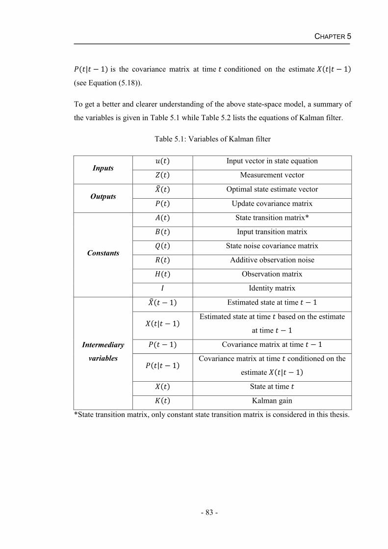
CHAPTER 5
- 83 -
( | 1) is the covariance matrix at time conditioned on the estimate ( | 1)(see Equation (5.18)).
To get a better and clearer understanding of the above state-space model, a summary of
the variables is given in Table 5.1 while Table 5.2 lists the equations of Kalman filter.
Table 5.1: Variables of Kalman filter
Inputs( ) Input vector in state equation( ) Measurement vector
Outputs( ) Optimal state estimate vector( ) Update covariance matrix
Constants
( ) State transition matrix*( ) Input transition matrix( ) State noise covariance matrix( ) Additive observation noise( ) Observation matrix
Identity matrix
Intermediary
variables
( 1) Estimated state at time 1( | 1) Estimated state at time based on the estimate
at time 1( 1) Covariance matrix at time 1( | 1) Covariance matrix at time conditioned on the
estimate ( | 1)( ) State at time ( ) Kalman gain
*State transition matrix, only constant state transition matrix is considered in this thesis.
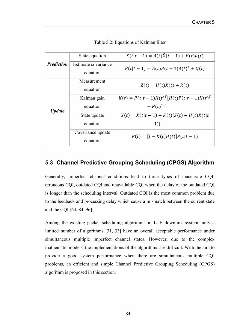
CHAPTER 5
- 84 -
Table 5.2: Equations of Kalman filter
Prediction
State equation ( | 1) = ( ) ( 1) + ( ) ( )Estimate covariance
equation( | 1) = ( ) ( 1) ( ) + ( )
Update
Measurement
equation( ) = ( ) ( ) + ( )
Kalman gain
equation
( ) = ( | 1) ( ) [ ( ) ( | 1) ( )+ ( )] 1State update
equation
( ) = ( | 1) + ( )[ ( ) ( ) ( |1)]Covariance update
equation( ) = [ ( ) ( )] ( | 1)
5.3 Channel Predictive Grouping Scheduling (CPGS) Algorithm
Generally, imperfect channel conditions lead to three types of inaccurate CQI:
erroneous CQI, outdated CQI and unavailable CQI when the delay of the outdated CQI
is longer than the scheduling interval. Outdated CQI is the most common problem due
to the feedback and processing delay which cause a mismatch between the current state
and the CQI [64, 84, 96].
Among the existing packet scheduling algorithms in LTE downlink system, only a
limited number of algorithms [31, 33] have an overall acceptable performance under
simultaneous multiple imperfect channel states. However, due to the complex
mathematic models, the implementations of the algorithms are difficult. With the aim to
provide a good system performance when there are simultaneous multiple CQI
problems, an efficient and simple Channel Predictive Grouping Scheduling (CPGS)
algorithm is proposed in this section.
CHAPTER 5
- 85 -
5.3.1 Kalman Filter for Channel Prediction
As an optimal autoregressive prediction method, Kalman filter has been applied to
channel condition prediction [94, 97, 98]. It is able to forecast the current channel state
from the previous state and hence an accurate CQI can be recovered from the erroneous
channel quality feedback. The classical Kalman filter method consists of two steps:
prediction and update. In the prediction step, the current CQI value is estimated from
the CQI in the last TTI while the estimated current CQI conditioned on last TTI is
improved according to the observed CQI value from each user’s CQI report in update
step. The equations are given below:
Prediction step: ( | 1) = ( ) ( 1) (5.23)
where ( | 1) is the estimated CQI at time based on the estimate at time 1.( ) is the transition matrix that connects two consecutive states, ( ) and ( 1),( 1) is the estimated CQI at time 1.( | 1) = ( ) ( 1) ( ) (5.24)
where ( | 1) is the covariance matrix of ( | 1) at time , ( ) is the
transposed matrix of ( ) and ( 1) is the covariance matrix of ( 1) at time 1 . The covariance matrix describes the estimation accuracy. The following
correction step is based on this parameter.
Update step: ( ) = ( ) ( ) + ( ) (5.25)
where ( ) is the measurement CQI vector at time , ( ) is the observation matrix at
time , ( ) is the received CQI vector at time and ( ) is the measurement error
covariance matrix at time . In our work, ( )is obtained directly from the CQI value
reported by each user.( ) = ( | 1) ( ) [ ( ) ( | 1) ( ) + ( )] 1 (5.26)
CHAPTER 5
- 86 -
where ( ) is the Kalman gain at time . Kalman gain can be regarded as a weight
parameter to update the estimated CQI ( | 1). It is an important indicator that can
be used to determine whether the initialization of the Kalman filter is appropriate. As
inappropriate initializations of Kalman filter may result in a value for ( ) that is
beyond its reasonable range (i.e. 0 < ( ) < 1) in the recursive process and may lead
to a failed convergence of Kalman filter towards a correct prediction.( ) = ( | 1) + ( )[ ( ) ( ) ( | 1)] (5.27)
where ( ) is the optimal estimated CQI vector at time . It is an update from the
previous estimate ( | 1)( ) = [ ( ) ( )] ( | 1) (5.28)
where ( ) is the updated covariance matrix and I is the identity matrix. The calculation
of ( ) is for the estimation in the next scheduling interval and the Kalman filter can
proceed recursively with ( ).
Figure 5.1 describes the process and the state-space equations of the Kalman filter.
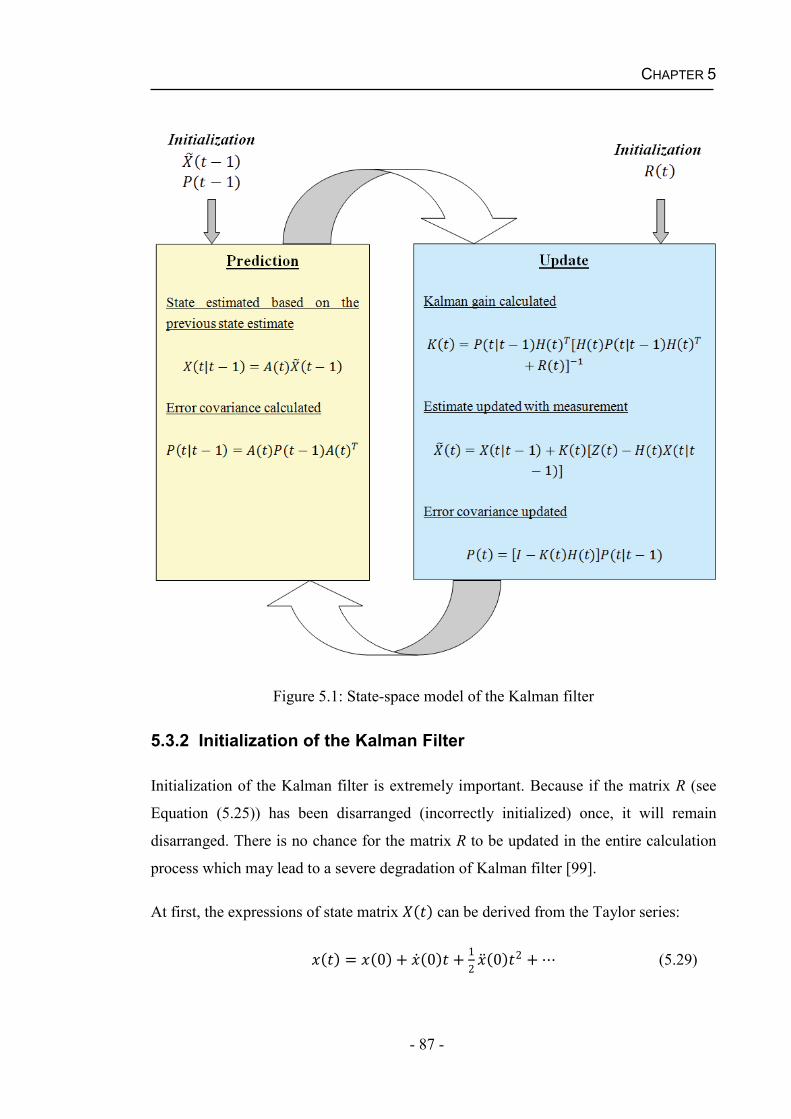
CHAPTER 5
- 87 -
Figure 5.1: State-space model of the Kalman filter
5.3.2 Initialization of the Kalman Filter
Initialization of the Kalman filter is extremely important. Because if the matrix R (see
Equation (5.25)) has been disarranged (incorrectly initialized) once, it will remain
disarranged. There is no chance for the matrix R to be updated in the entire calculation
process which may lead to a severe degradation of Kalman filter [99].
At first, the expressions of state matrix ( ) can be derived from the Taylor series:
( ) = (0) + (0) + 12 (0) 2 + (5.29)
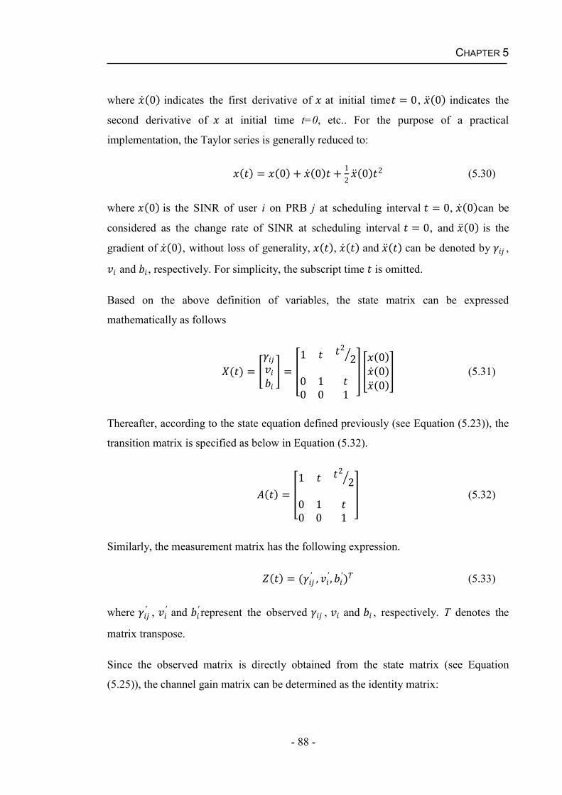
CHAPTER 5
- 88 -
where (0) indicates the first derivative of at initial time = 0, (0) indicates the
second derivative of at initial time t=0, etc.. For the purpose of a practical
implementation, the Taylor series is generally reduced to:
( ) = (0) + (0) + 12 (0) 2 (5.30)
where (0) is the SINR of user i on PRB j at scheduling interval = 0, (0)can be
considered as the change rate of SINR at scheduling interval = 0, and (0) is the
gradient of (0), without loss of generality, ( ), ( ) and ( ) can be denoted by ,
and , respectively. For simplicity, the subscript time is omitted.
Based on the above definition of variables, the state matrix can be expressed
mathematically as follows
( ) = = 1 2 20 10 0 1(0)(0)(0) (5.31)
Thereafter, according to the state equation defined previously (see Equation (5.23)), the
transition matrix is specified as below in Equation (5.32).
( ) = 1 2 20 10 0 1 (5.32)
Similarly, the measurement matrix has the following expression.( ) = ( , , ) (5.33)
where , and represent the observed , and , respectively. T denotes the
matrix transpose.
Since the observed matrix is directly obtained from the state matrix (see Equation
(5.25)), the channel gain matrix can be determined as the identity matrix:
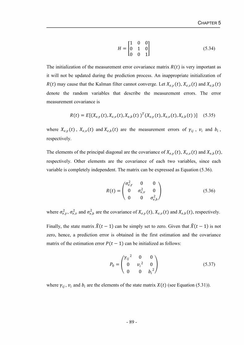
CHAPTER 5
- 89 -
= 1 0 00 1 00 0 1 (5.34)
The initialization of the measurement error covariance matrix ( ) is very important as
it will not be updated during the prediction process. An inappropriate initialization of ( ) may cause that the Kalman filter cannot converge. Let , ( ), , ( ) and , ( )denote the random variables that describe the measurement errors. The error
measurement covariance is ( ) = [( , ( ), , ( ), , ( ) ) ( , ( ), , ( ), , ( ) )] (5.35)
where , ( ) , , ( ) and , ( ) are the measurement errors of , and ,
respectively.
The elements of the principal diagonal are the covariance of , ( ), , ( ) and , ( ),
respectively. Other elements are the covariance of each two variables, since each
variable is completely independent. The matrix can be expressed as Equation (5.36).
( ) = ,2 0 00 ,2 00 0 ,2 (5.36)
where ,2 , ,2 and ,2 are the covariance of , ( ), , ( ) and , ( ), respectively.
Finally, the state matrix ( 1) can be simply set to zero. Given that ( 1) is not
zero, hence, a prediction error is obtained in the first estimation and the covariance
matrix of the estimation error ( 1) can be initialized as follows:
0 = 2 0 00 2 00 0 2 (5.37)
where , and are the elements of the state matrix ( ) (see Equation (5.31)).
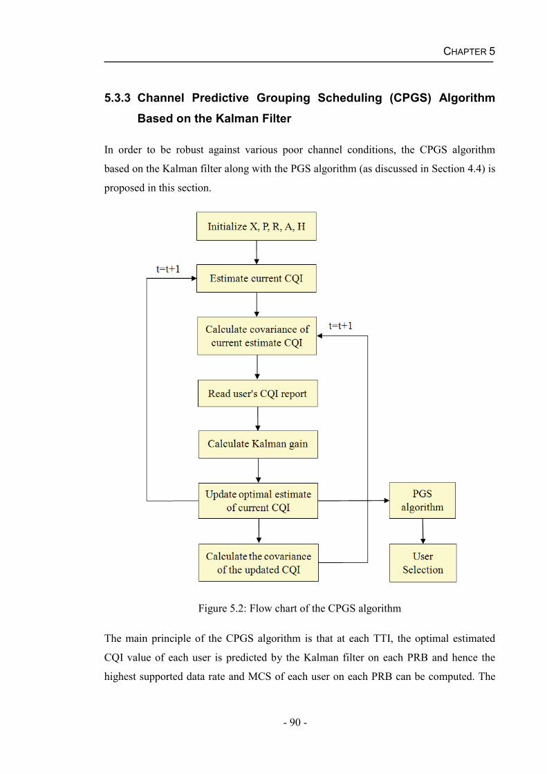
CHAPTER 5
- 90 -
5.3.3 Channel Predictive Grouping Scheduling (CPGS) Algorithm Based on the Kalman Filter
In order to be robust against various poor channel conditions, the CPGS algorithm
based on the Kalman filter along with the PGS algorithm (as discussed in Section 4.4) is
proposed in this section.
Figure 5.2: Flow chart of the CPGS algorithm
The main principle of the CPGS algorithm is that at each TTI, the optimal estimated
CQI value of each user is predicted by the Kalman filter on each PRB and hence the
highest supported data rate and MCS of each user on each PRB can be computed. The
CHAPTER 5
- 91 -
estimated CQI, corresponding data rate and the MCS are used by the PGS algorithm (as
proposed in Section 4.4.1) to make the scheduling decision.
Based on the above analysis, the proposed packet scheduling algorithm is described in
Figure 5.2.
5.4 Results and Discussions
In the earlier research work, it was assumed that the eNB has a perfect knowledge of
CQI and all packets are received correctly at the UE. However, a more practical
simulation environment is considered in this section. Additional parameter settings
(apart from Section 2.7) are made for the imperfect channel conditions in this section: i)
a combination of multiple imperfect CQI types was assumed in this simulation. Each
CQI report has a 3 ms delay and becomes unavailable at a regular interval (10 ms), ii)
packets may be received incorrectly at UE, so a HARQ technique was employed (as
discussed in Section 2.4), iii) based on the 3GPP recommendation [26], the GBR PLR
threshold was set to 10 2 while the threshold of the GBR average system buffer delay
was capped at 80 ms.
Four performance metrics were used to evaluate the performance: system throughput,
fairness, PLR and average system delay. To compare the QoS of GBR services under
multiple speed scenarios, user velocity was set to 3 km/h and 30 km/h. The detailed
simulation parameters are listed in Table 5.3.
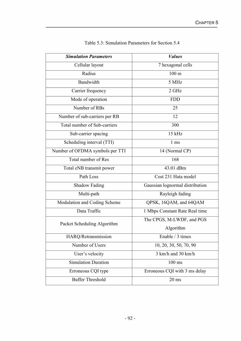
CHAPTER 5
- 92 -
Table 5.3: Simulation Parameters for Section 5.4
Simulation Parameters Values
Cellular layout 7 hexagonal cells
Radius 100 m
Bandwidth 5 MHz
Carrier frequency 2 GHz
Mode of operation FDD
Number of RBs 25
Number of sub-carriers per RB 12
Total number of Sub-carriers 300
Sub-carrier spacing 15 kHz
Scheduling interval (TTI) 1 ms
Number of OFDMA symbols per TTI 14 (Normal CP)
Total number of Res 168
Total eNB transmit power 43.01 dBm
Path Loss Cost 231 Hata model
Shadow Fading Gaussian lognormal distribution
Multi-path Rayleigh fading
Modulation and Coding Scheme QPSK, 16QAM, and 64QAM
Data Traffic 1 Mbps Constant Rate Real time
Packet Scheduling AlgorithmThe CPGS, M-LWDF, and PGS
Algorithm
HARQ/Retransmission Enable / 3 times
Number of Users 10, 20, 30, 50, 70, 90
User’s velocity 3 km/h and 30 km/h
Simulation Duration 100 ms
Erroneous CQI type Erroneous CQI with 3 ms delay
Buffer Threshold 20 ms
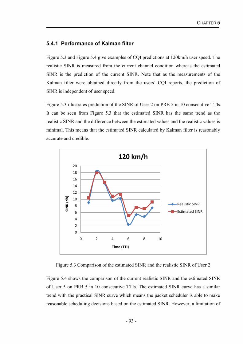
CHAPTER 5
- 93 -
5.4.1 Performance of Kalman filter
Figure 5.3 and Figure 5.4 give examples of CQI predictions at 120km/h user speed. The
realistic SINR is measured from the current channel condition whereas the estimated
SINR is the prediction of the current SINR. Note that as the measurements of the
Kalman filter were obtained directly from the users’ CQI reports, the prediction of
SINR is independent of user speed.
Figure 5.3 illustrates prediction of the SINR of User 2 on PRB 5 in 10 consecutive TTIs.
It can be seen from Figure 5.3 that the estimated SINR has the same trend as the
realistic SINR and the difference between the estimated values and the realistic values is
minimal. This means that the estimated SINR calculated by Kalman filter is reasonably
accurate and credible.
Figure 5.3 Comparison of the estimated SINR and the realistic SINR of User 2
Figure 5.4 shows the comparison of the current realistic SINR and the estimated SINR
of User 5 on PRB 5 in 10 consecutive TTIs. The estimated SINR curve has a similar
trend with the practical SINR curve which means the packet scheduler is able to make
reasonable scheduling decisions based on the estimated SINR. However, a limitation of
0
2
4
6
8
10
12
14
16
18
20
0 2 4 6 8 10
SIN
R (d
b)
Time (TTI)
120 km/h
Realistic SINR
Estimated SINR

CHAPTER 5
- 94 -
the Kalman filter is shown in Figure 5.4. In the last few TTIs, the estimations are not
accurate enough when the true values increase or decrease dramatically.
Figure 5.4: Comparison of the estimated SINR and the realistic SINR of User 5
In order to have an overall evaluation of the Kalman filter, 500 sample estimated SINRs
were compared with the correct values in a 100 ms simulation interval. In this
simulation, an imperfect channel condition was assumed where the practical SINR was
unable to be measured at a regular interval (10 ms). To evaluate the impact of the
Kalman filter on packet scheduling algorithm, the estimated instantaneous SINR was
mapped into CQI values and the differences between the estimated CQI and the correct
CQI (hereafter referred to as estimation error) were calculated. Note that the CQI is an
integer as described in Table 2.2.
It is shown in Figure 5.5 that 56% of the SINR estimations are correct (i.e. the
difference between the estimated CQI and the correct CQI is zero), and 33.6% of the
estimation errors are one. This means approximately 90% of the estimation errors are
less than or equal to one. The maximum estimation error is three and only 0.8% of the
SINR estimations are in this category. The simulation results proved that the Kalman
0
2
4
6
8
10
12
14
16
18
20
0 2 4 6 8 10
SIN
R (d
b)
Time (TTI)
120 km/h
Realistic SINR
Estimated SINR
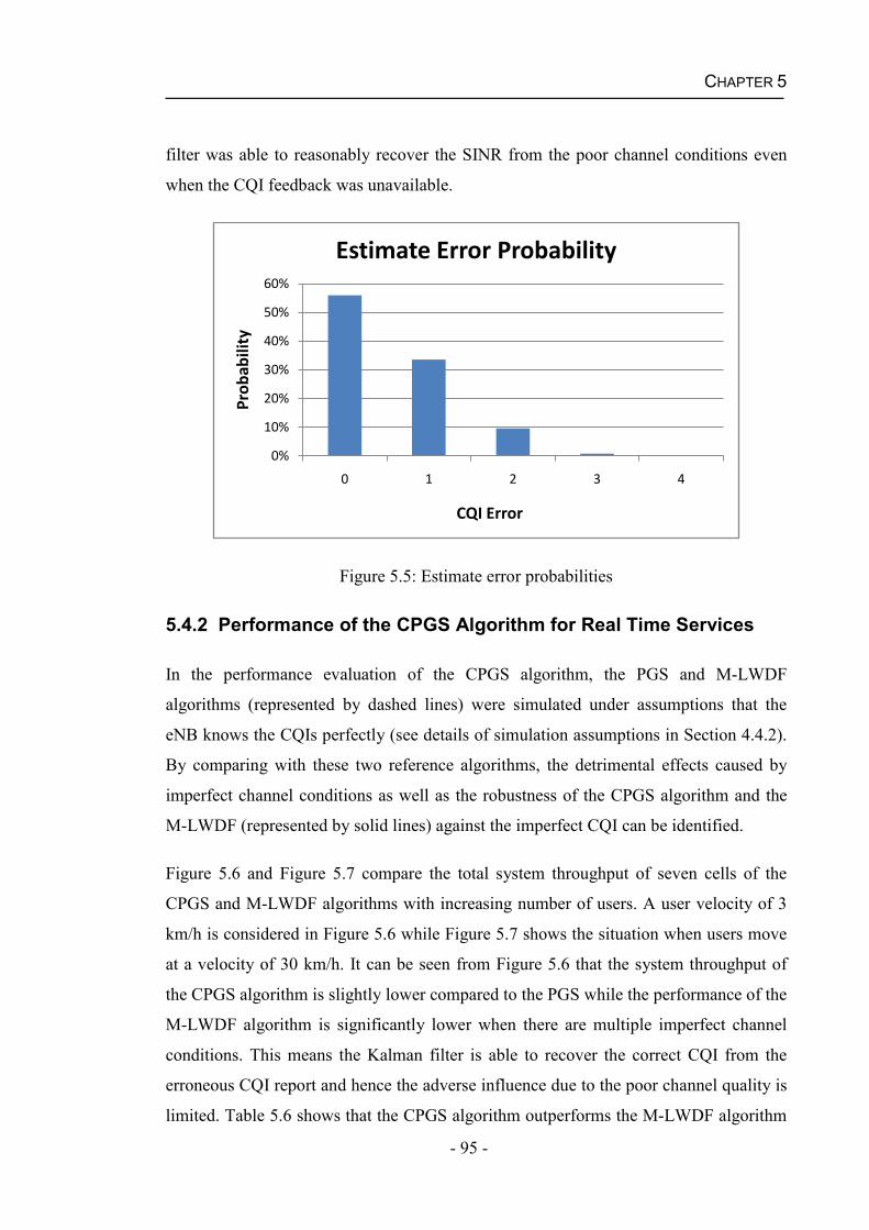
CHAPTER 5
- 95 -
filter was able to reasonably recover the SINR from the poor channel conditions even
when the CQI feedback was unavailable.
Figure 5.5: Estimate error probabilities
5.4.2 Performance of the CPGS Algorithm for Real Time Services
In the performance evaluation of the CPGS algorithm, the PGS and M-LWDF
algorithms (represented by dashed lines) were simulated under assumptions that the
eNB knows the CQIs perfectly (see details of simulation assumptions in Section 4.4.2).
By comparing with these two reference algorithms, the detrimental effects caused by
imperfect channel conditions as well as the robustness of the CPGS algorithm and the
M-LWDF (represented by solid lines) against the imperfect CQI can be identified.
Figure 5.6 and Figure 5.7 compare the total system throughput of seven cells of the
CPGS and M-LWDF algorithms with increasing number of users. A user velocity of 3
km/h is considered in Figure 5.6 while Figure 5.7 shows the situation when users move
at a velocity of 30 km/h. It can be seen from Figure 5.6 that the system throughput of
the CPGS algorithm is slightly lower compared to the PGS while the performance of the
M-LWDF algorithm is significantly lower when there are multiple imperfect channel
conditions. This means the Kalman filter is able to recover the correct CQI from the
erroneous CQI report and hence the adverse influence due to the poor channel quality is
limited. Table 5.6 shows that the CPGS algorithm outperforms the M-LWDF algorithm
0%
10%
20%
30%
40%
50%
60%
0 1 2 3 4
Prob
abili
ty
CQI Error
Estimate Error Probability
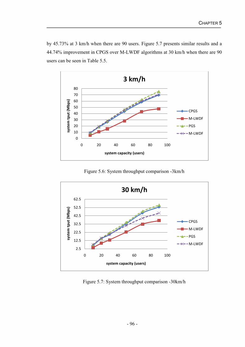
CHAPTER 5
- 96 -
by 45.73% at 3 km/h when there are 90 users. Figure 5.7 presents similar results and a
44.74% improvement in CPGS over M-LWDF algorithms at 30 km/h when there are 90
users can be seen in Table 5.5.
Figure 5.6: System throughput comparison -3km/h
Figure 5.7: System throughput comparison -30km/h
0
10
20
30
40
50
60
70
80
0 20 40 60 80 100
syst
em tp
ut (M
bps)
system capacity (users)
3 km/h
CPGS
M-LWDF
PGS
M-LWDF
2.5
12.5
22.5
32.5
42.5
52.5
62.5
0 20 40 60 80 100
syst
em tp
ut (M
bps)
system capacity (users)
30 km/h
CPGS
M-LWDF
PGS
M-LWDF
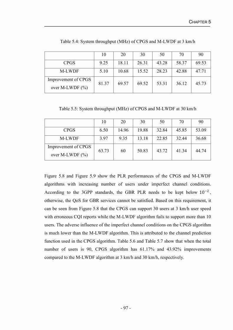
CHAPTER 5
- 97 -
Table 5.4: System throughput (MHz) of CPGS and M-LWDF at 3 km/h
10 20 30 50 70 90
CPGS 9.25 18.11 26.31 43.28 58.37 69.53
M-LWDF 5.10 10.68 15.52 28.23 42.88 47.71
Improvement of CPGS
over M-LWDF (%)81.37 69.57 69.52 53.31 36.12 45.73
Table 5.5: System throughput (MHz) of CPGS and M-LWDF at 30 km/h
10 20 30 50 70 90
CPGS 6.50 14.96 19.88 32.84 45.85 53.09
M-LWDF 3.97 9.35 13.18 22.85 32.44 36.68
Improvement of CPGS
over M-LWDF (%)63.73 60 50.83 43.72 41.34 44.74
Figure 5.8 and Figure 5.9 show the PLR performances of the CPGS and M-LWDF
algorithms with increasing number of users under imperfect channel conditions.
According to the 3GPP standards, the GBR PLR needs to be kept below 10 2 ,
otherwise, the QoS for GBR services cannot be satisfied. Based on this requirement, it
can be seen from Figure 5.8 that the CPGS can support 30 users at 3 km/h user speed
with erroneous CQI reports while the M-LWDF algorithm fails to support more than 10
users. The adverse influence of the imperfect channel conditions on the CPGS algorithm
is much lower than the M-LWDF algorithm. This is attributed to the channel prediction
function used in the CPGS algorithm. Table 5.6 and Table 5.7 show that when the total
number of users is 90, CPGS algorithm has 61.17% and 43.92% improvements
compared to the M-LWDF algorithm at 3 km/h and 30 km/h, respectively.
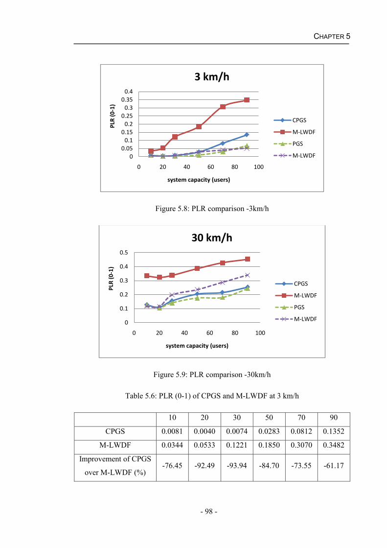
CHAPTER 5
- 98 -
Figure 5.8: PLR comparison -3km/h
Figure 5.9: PLR comparison -30km/h
Table 5.6: PLR (0-1) of CPGS and M-LWDF at 3 km/h
10 20 30 50 70 90
CPGS 0.0081 0.0040 0.0074 0.0283 0.0812 0.1352
M-LWDF 0.0344 0.0533 0.1221 0.1850 0.3070 0.3482
Improvement of CPGS
over M-LWDF (%)-76.45 -92.49 -93.94 -84.70 -73.55 -61.17
00.05
0.10.15
0.20.25
0.30.35
0.4
0 20 40 60 80 100
PLR
(0-1
)
system capacity (users)
3 km/h
CPGS
M-LWDF
PGS
M-LWDF
0
0.1
0.2
0.3
0.4
0.5
0 20 40 60 80 100
PLR
(0-1
)
system capacity (users)
30 km/h
CPGS
M-LWDF
PGS
M-LWDF
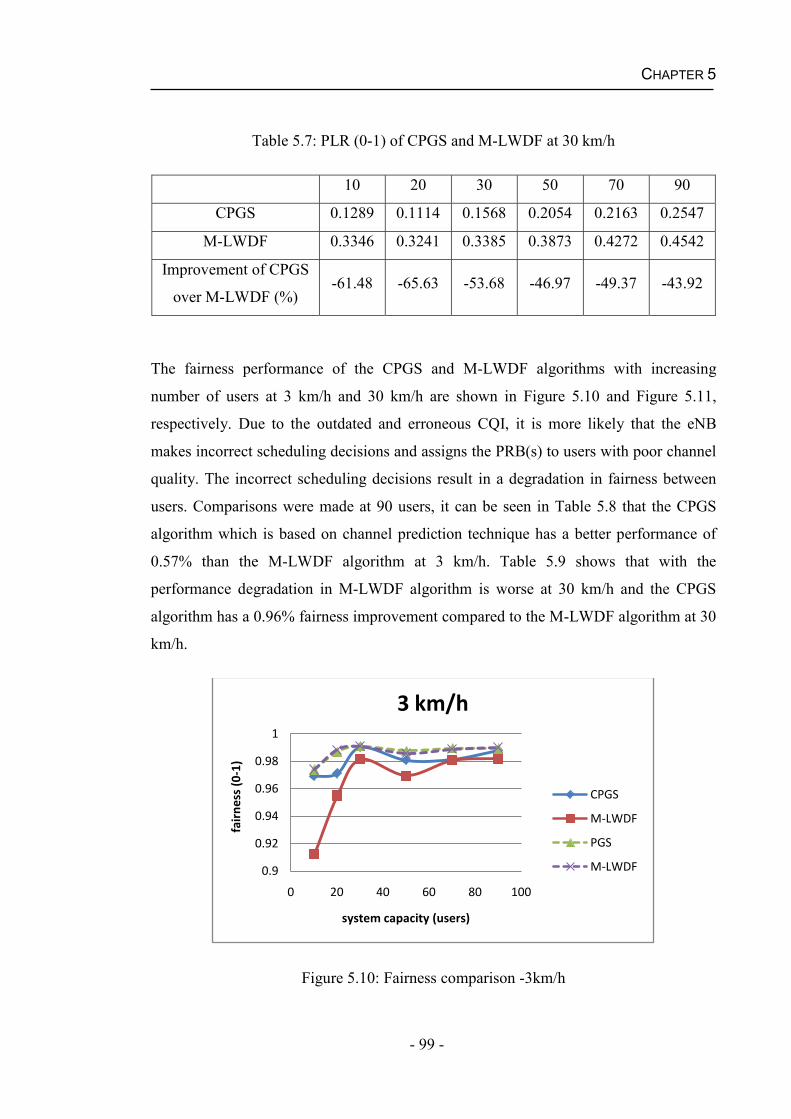
CHAPTER 5
- 99 -
Table 5.7: PLR (0-1) of CPGS and M-LWDF at 30 km/h
10 20 30 50 70 90
CPGS 0.1289 0.1114 0.1568 0.2054 0.2163 0.2547
M-LWDF 0.3346 0.3241 0.3385 0.3873 0.4272 0.4542
Improvement of CPGS
over M-LWDF (%)-61.48 -65.63 -53.68 -46.97 -49.37 -43.92
The fairness performance of the CPGS and M-LWDF algorithms with increasing
number of users at 3 km/h and 30 km/h are shown in Figure 5.10 and Figure 5.11,
respectively. Due to the outdated and erroneous CQI, it is more likely that the eNB
makes incorrect scheduling decisions and assigns the PRB(s) to users with poor channel
quality. The incorrect scheduling decisions result in a degradation in fairness between
users. Comparisons were made at 90 users, it can be seen in Table 5.8 that the CPGS
algorithm which is based on channel prediction technique has a better performance of
0.57% than the M-LWDF algorithm at 3 km/h. Table 5.9 shows that with the
performance degradation in M-LWDF algorithm is worse at 30 km/h and the CPGS
algorithm has a 0.96% fairness improvement compared to the M-LWDF algorithm at 30
km/h.
Figure 5.10: Fairness comparison -3km/h
0.9
0.92
0.94
0.96
0.98
1
0 20 40 60 80 100
fair
ness
(0-1
)
system capacity (users)
3 km/h
CPGS
M-LWDF
PGS
M-LWDF
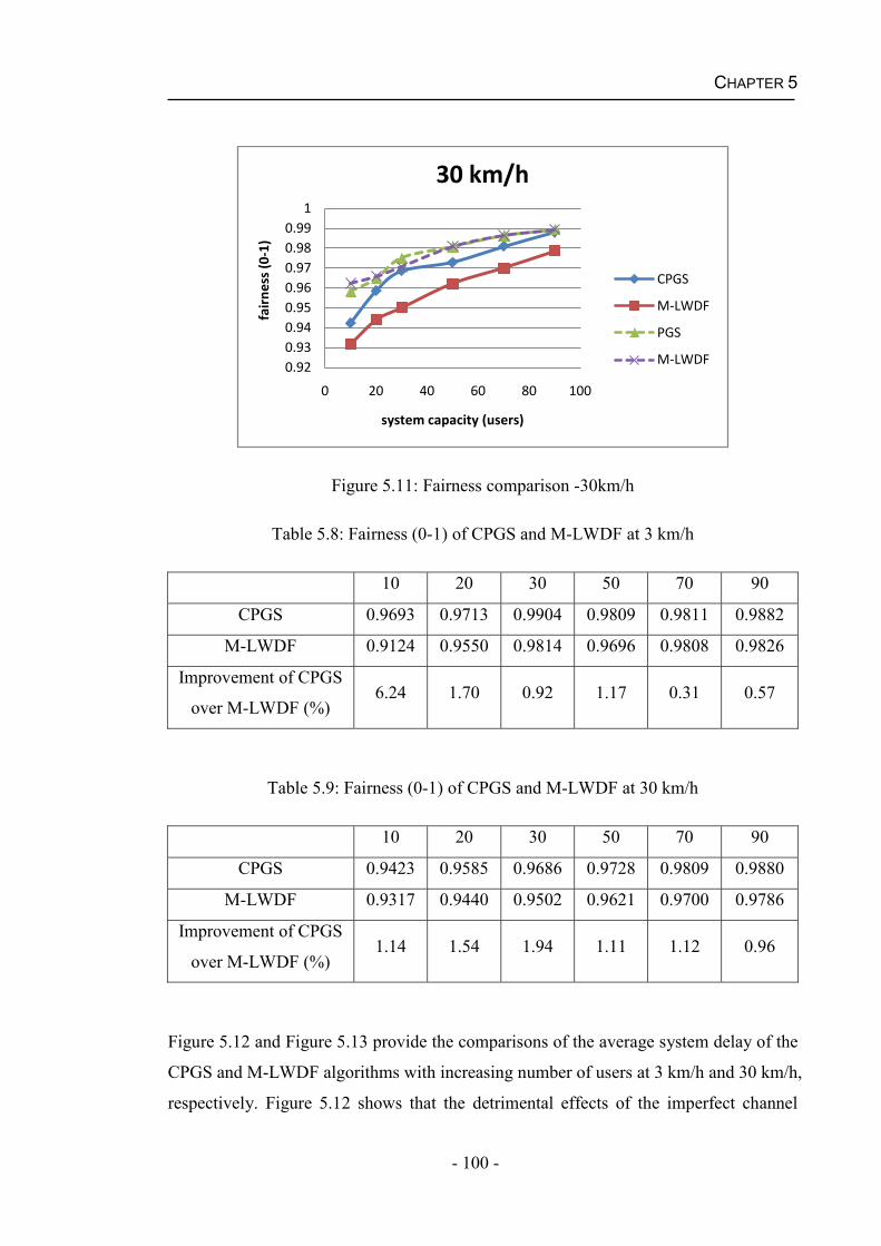
CHAPTER 5
- 100 -
Figure 5.11: Fairness comparison -30km/h
Table 5.8: Fairness (0-1) of CPGS and M-LWDF at 3 km/h
10 20 30 50 70 90
CPGS 0.9693 0.9713 0.9904 0.9809 0.9811 0.9882
M-LWDF 0.9124 0.9550 0.9814 0.9696 0.9808 0.9826
Improvement of CPGS
over M-LWDF (%)6.24 1.70 0.92 1.17 0.31 0.57
Table 5.9: Fairness (0-1) of CPGS and M-LWDF at 30 km/h
10 20 30 50 70 90
CPGS 0.9423 0.9585 0.9686 0.9728 0.9809 0.9880
M-LWDF 0.9317 0.9440 0.9502 0.9621 0.9700 0.9786
Improvement of CPGS
over M-LWDF (%)1.14 1.54 1.94 1.11 1.12 0.96
Figure 5.12 and Figure 5.13 provide the comparisons of the average system delay of the
CPGS and M-LWDF algorithms with increasing number of users at 3 km/h and 30 km/h,
respectively. Figure 5.12 shows that the detrimental effects of the imperfect channel
0.920.930.940.950.960.970.980.99
1
0 20 40 60 80 100
fair
ness
(0-1
)
system capacity (users)
30 km/h
CPGS
M-LWDF
PGS
M-LWDF
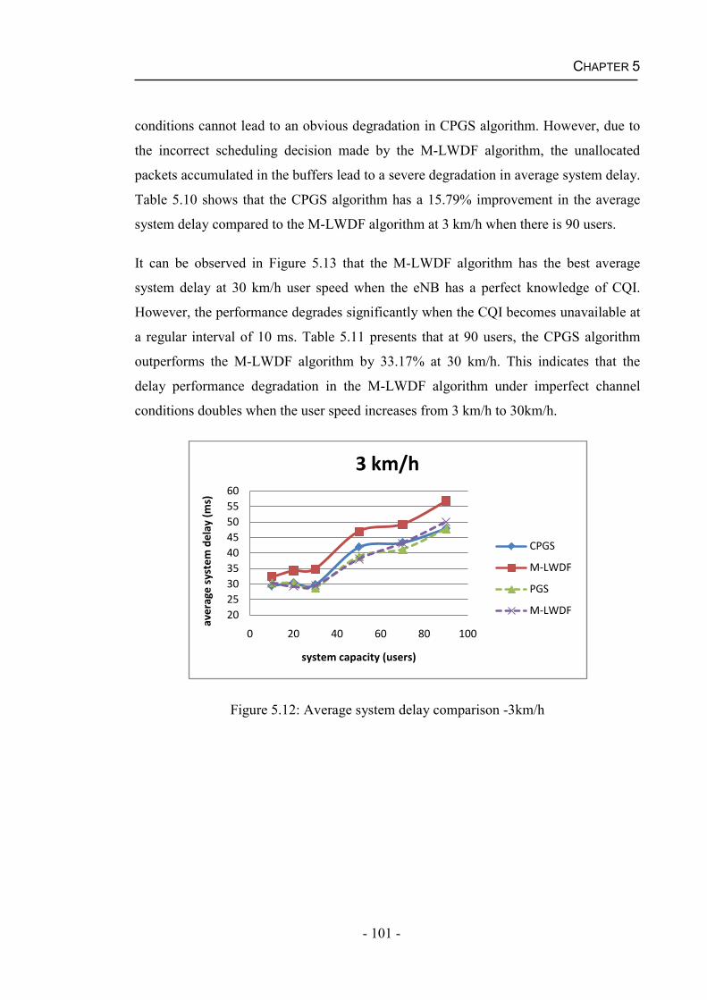
CHAPTER 5
- 101 -
conditions cannot lead to an obvious degradation in CPGS algorithm. However, due to
the incorrect scheduling decision made by the M-LWDF algorithm, the unallocated
packets accumulated in the buffers lead to a severe degradation in average system delay.
Table 5.10 shows that the CPGS algorithm has a 15.79% improvement in the average
system delay compared to the M-LWDF algorithm at 3 km/h when there is 90 users.
It can be observed in Figure 5.13 that the M-LWDF algorithm has the best average
system delay at 30 km/h user speed when the eNB has a perfect knowledge of CQI.
However, the performance degrades significantly when the CQI becomes unavailable at
a regular interval of 10 ms. Table 5.11 presents that at 90 users, the CPGS algorithm
outperforms the M-LWDF algorithm by 33.17% at 30 km/h. This indicates that the
delay performance degradation in the M-LWDF algorithm under imperfect channel
conditions doubles when the user speed increases from 3 km/h to 30km/h.
Figure 5.12: Average system delay comparison -3km/h
202530354045505560
0 20 40 60 80 100
aver
age
syst
em d
elay
(ms)
system capacity (users)
3 km/h
CPGS
M-LWDF
PGS
M-LWDF
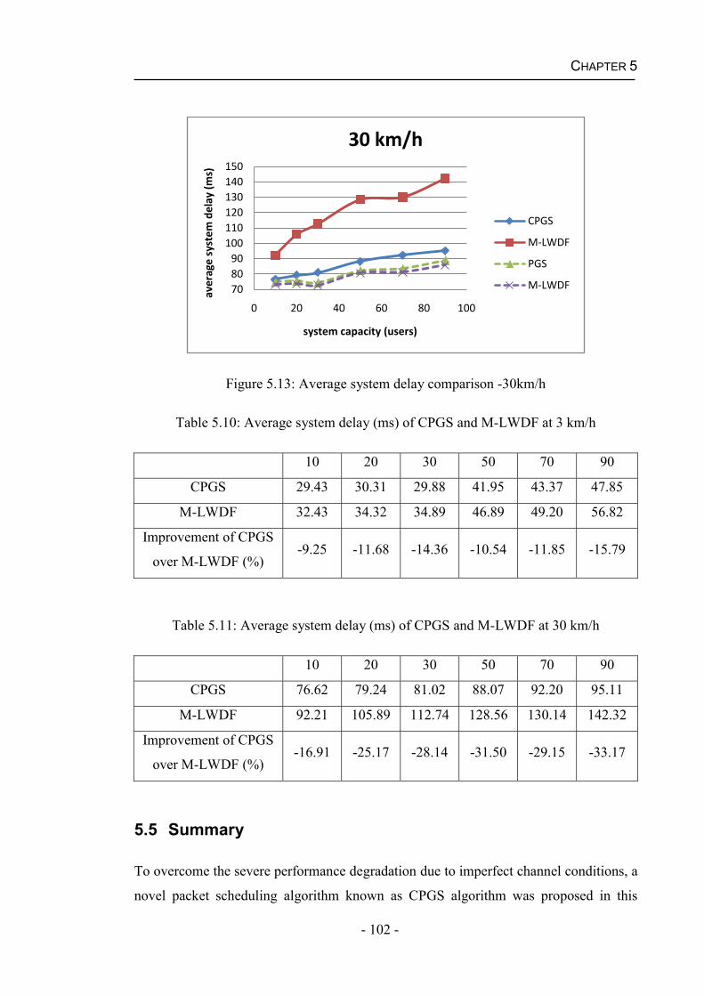
CHAPTER 5
- 102 -
Figure 5.13: Average system delay comparison -30km/h
Table 5.10: Average system delay (ms) of CPGS and M-LWDF at 3 km/h
10 20 30 50 70 90
CPGS 29.43 30.31 29.88 41.95 43.37 47.85
M-LWDF 32.43 34.32 34.89 46.89 49.20 56.82
Improvement of CPGS
over M-LWDF (%)-9.25 -11.68 -14.36 -10.54 -11.85 -15.79
Table 5.11: Average system delay (ms) of CPGS and M-LWDF at 30 km/h
10 20 30 50 70 90
CPGS 76.62 79.24 81.02 88.07 92.20 95.11
M-LWDF 92.21 105.89 112.74 128.56 130.14 142.32
Improvement of CPGS
over M-LWDF (%)-16.91 -25.17 -28.14 -31.50 -29.15 -33.17
5.5 Summary
To overcome the severe performance degradation due to imperfect channel conditions, a
novel packet scheduling algorithm known as CPGS algorithm was proposed in this
708090
100110120130140150
0 20 40 60 80 100
aver
age
syst
em d
elay
(ms)
system capacity (users)
30 km/h
CPGS
M-LWDF
PGS
M-LWDF
CHAPTER 5
- 103 -
chapter to provide satisfactory QoS for real time applications in the downlink LTE
systems. The algorithm consists of two phases: the channel prediction and the packet
scheduling. The channel prediction phase estimates the CQI of each user using a
Kalman filter based channel predictor. The packet scheduling phase employs the PGS
algorithm to make scheduling decisions based on the estimated CQI from the channel
predictor.
Based on the simulation results, it can be concluded that under imperfect channel
conditions, the CPGS algorithm significantly increases the system throughput and
fairness and at the same time decreases the PLR and average system delay when
compared to the M-LWDF algorithm.
A system level simulation was developed for imperfect channel conditions and used for
evaluating the performance of the CPGS and M-LWDF algorithms. The simulation
results show that the CPGS algorithm maintains a good and stable scheduling capacity
while the performances of the M-LWDF algorithms degrade significantly due to the
erroneous CQI feedback.
- 104 -
Chapter 6
CONCLUSIONS AND FUTURE RESEARCH DIRECTIONS
A number of challenges in designing packet scheduling algorithms under time-varying
channel conditions were presented in this thesis. Given the research gaps, some
contributions were made to improve performance of packet scheduling algorithms in the
downlink LTE. This chapter summarizes the original contributions of this thesis and
listed relevant study directions for future work.
6.1 Summary of Thesis Contributions
The original contributions consist of two major areas as follows:
6.1.1 Providing an overall good performance to support QoS
To provide satisfactory QoS for GBR services, a packet scheduling scheme referred to
as QOGS that aims to achieve the best overall performance and be robust against the
time-varying channel environments was proposed. Based on the QOGS scheme, a
scheduling algorithm namely PGS was proposed to address the research question: “Is it
possible to develop a new packet scheduling algorithm for the downlink LTE that can
offer an overall good system performance and at the same time maintain a low
computational cost? If so, how much performance improvement does the new algorithm
offer over conventional packet scheduling algorithms?”
A system level simulation assuming 3 ms delay in each CQI report was conducted to
evaluate the performance of the PGS algorithm at user speeds of 3 km/h and 30 km/h. It
was proved by the results that the PGS algorithm outperforms M-LWDF algorithm in
terms of system throughput and PLR at 3 km/h by 7% and 38.89%, respectively. At 30
km/h, the PGS algorithm achieved an improvement in system throughput over M-
LWDF algorithm by 21.37% while 10.53% better average system delay was achieved
by the PGS algorithm compared to the Max Rate algorithm.
CHAPTER 6
- 105 -
6.1.2 Providing Robust Performance under Imperfect Channel Conditions
A mathematic model of Kalman filter for channel condition prediction was developed in
Chapter 5. By using the Kalman filter based channel predictor, the correct CQI was
recovered from the erroneous channel quality feedback. A system level simulation was
performed under imperfect channel conditions (see Section 5.4.1 for detailed simulation
assumptions). It was presented via the simulation that approximately 90% of the
estimation errors are controlled below one.
A Kalman filter based packet scheduling algorithm called CPGS was proposed in
Chapter 5 to address the research question:“In the presence of various practical
imperfect CQI, is it possible to propose a packet scheduling algorithm based on channel
prediction with low computational complexity to adapt to multiple the imperfect
channel states? If so, how much performance improvement does the new algorithm
offer over conventional packet scheduling algorithms?”
Under the imperfect channel conditions (see Section 5.4.2 for detailed simulation
assumptions), the CPGS algorithm outperforms the M-LWDF algorithm at 3 km/h in
terms of system throughput, PLR, fairness and average system delay by 45.73%,
61.17%, 0.57% and 15.79%, respectively. And at 30 km/h, the improvements are
44.74 %, 43.92%, 0.96% and 33.17%, respectively. Based on the simulation results, it
can be concluded that the CPGS algorithm maintains a good and stable scheduling
capacity while the performances of the M-LWDF algorithms degrade significantly due
to the erroneous CQI feedback.
6.2 Future Research Directions
Based on the current research study and the challenges in packet scheduling, some of
the identified research directions are briefly summarized as follows:
i) The majority of works in this thesis focus on the GBR services. To make an overall
performance evaluation of packet scheduling algorithms, Non-GBR services will be
considered in the designing of packet scheduling algorithms for future study.
CHAPTER 6
- 106 -
ii) Imperfect channel conditions include outdated CQI, erroneous CQI, unavailable
CQI, inappropriate CQI reporting rate, channel estimation error, etc. Due to time
limitation, the current works only focus on the outdated CQI and unavailable CQI.
New packet scheduling algorithms will be developed in future research work to
address the detrimental effects due to more sources of the impairment.
iii) To reduce the complexity of the simulation, some assumptions were applied in the
thesis. For instance, the constant bit rate traffic model and the constant inter-cell
interference. Future study will investigate the performance of packet scheduling
algorithms based on some more practical multimedia applications such as video
streaming, web browsing, etc..
- 107 -
REFERENCES
[1] E. Dahlman, S. Parkvall, J. Skold, and P. Beming, 3G evolution: HSPA and LTE for mobile broadband: Academic Press, 2010.
[2] B. Sanou, "ICT Facts and Figures," International Telecommunications Union, 2013.
[3] E. Dahlman, "3G long-term evolution," Ericsson Research, 2007.[4] T. Halonen, J. Romero, and J. Melero, GSM, GPRS and EDGE performance:
evolution towards 3G/UMTS: Wiley. com, 2004.[5] UMTS. World, "The Hisory of UMTS and 3G Development,"
in http://www.umtsworld.com/umts/history.htm, accessed: 23 September 2013.[6] A. Samukic, "UMTS universal mobile telecommunications system: development
of standards for the third generation," in Global Telecommunications Conference, 1998. GLOBECOM 1998. The Bridge to Global Integration. IEEE,1998, pp. 1976-1983.
[7] Wikipedia, "LTE Timeline," in http://en.wikipedia.org/wiki/LTE_timeline,accessed: 30 September 2013.
[8] A. Technologies, "3GPP LTE: Introducing Single-Carrier FDMA," in http://cp.literature.agilent.com/litweb/pdf/5989-7898EN.pdf, accessed: 23 September 2013.
[9] YOTA. (2012, "Yota Networks has launched the world's first mobile communication technology LTE Advanced," in http://www.yota.ru/ru/news/details/?ID=316537, accessed: 23 September 2013.
[10] T. I. (2011), "Short and Long-Term Visions of 4G," in http://trends-in-telecoms.blogspot.com.au/2011/07/short-and-long-term-visions-of-4g.html,accessed: 23 September 2013.
[11] G. RP-090604, "Draft Minutes (V4.0.1) of the 43rd 3GPP TSG RAN meeting," in MCC, 2001.
[12] A. M. Rao, A. Weber, S. Gollamudi, and R. Soni, "LTE and HSPA+: Revolutionary and evolutionary solutions for global mobile broadband," Bell Labs Technical Journal, vol. 13, pp. 7-34, 2009.
[13] H. G. Myung and D. Goodman, Single carrier FDMA: a new air interface for long term evolution vol. 8: Wiley, 2008.
[14] P. Beming, L. Frid, G. Hall, P. Malm, T. Noren, M. Olsson, and G. Rune, "LTE-SAE architecture and performance," Ericsson Review, vol. 20, pp. 98-104, 2007.
[15] 3GPP, "Evolved Universal Terrestrial Radio Access (E-UTRA) and EvolvedUniversal Terrestrial Radio Access Network (E-UTRAN); Overall Description;Stage 2 (Release 9)," TS 36.300, version 9.2.0, December 2009.
[16] A. K. S. Krishnarajah, "Mobile Communication Systems - Long Term Evolution.," in University of Technology, Sydney: Sydney, 2008.
REFERENCES
- 108 -
[17] A. Hadden, "Mobile broadband-where the next generation leads us [industry perspectives]," Wireless Communications, IEEE, vol. 16, pp. 6-9, 2009.
[18] 3GPP, "Requirements for Evolved UTRA (E-UTRA) and Evolved UTRAN (EUTRAN)(Release 7)," March 2006, TR25.913, version 7.3.0.
[19] Qualcomm, "3GPP Long-Term Evolution," in Qualcomm Incorporated, January 2008.
[20] L. Wieweg, "UMTS/LTE Flexible Capacity within the Harmonised Bands," in Ericsson LTE Warsaw, June 2007.
[21] Agilent. Application. Note, "3GPP Long Term Evolution: System Overview, ProductDevelopment, and Test Challenges," Literature Number, 2009.
[22] Anritsu, "LTE Resource Guide," inhttp://web.cecs.pdx.edu/~fli/class/LTE_Reource_Guide.pdf, accessed: 13 September 2013.
[23] H. A. M. Ramli, "Performance Analysis of Packet Schedulingin Long Term Evolution (LTE)," Doctor of Philosophy, Faculty of Engineering and Information Technology, University of Technology, Sydney, Australia, 2011.
[24] S. Stefania, T. Issam, and B. Matthew, "LTE-The UMTS long term evolution from theory to practice," A John Wiley and Sons, Ltd, 2009.
[25] G. Piro, L. A. Grieco, G. Boggia, F. Capozzi, and P. Camarda, "Simulating LTE cellular systems: an open-source framework," Vehicular Technology, IEEE Transactions on, vol. 60, pp. 498-513, 2011.
[26] 3GPP, "Policy and Charging Control Architecture (Release 9)," TS 23.203, version 9.3.0, December 2009.
[27] J. Gross, H. Karl, F. Fitzek, and A. Wolisz, "Comparison of heuristic and optimal subcarrier assignment algorithms," in Proc. of Intl. Conf. on Wireless Networks (ICWN), 2003.
[28] A. K. Khattab and K. M. Elsayed, "Opportunistic scheduling of delay sensitive traffic in ofdma-basedwireless," in proceedings of the 2006 International Symposium on on World of Wireless, Mobile and Multimedia Networks, 2006, pp. 279-288.
[29] M. R. Souryal and R. L. Pickholtz, "Adaptive modulation with imperfect channel information in OFDM," in Communications, 2001. ICC 2001. IEEE International Conference on, 2001, pp. 1861-1865 vol.6.
[30] H. A. M. Ramli, "Packet Scheduling Algorithm for the Future Wireless Systems," 2009, University of Technology Sydney, Sydney.
[31] I. C. Wong and B. Evans, "Optimal resource allocation in the OFDMA downlink with imperfect channel knowledge," Communications, IEEE Transactions on, vol. 57, pp. 232-241, 2009.
[32] D. S. W. Hui and V. K. N. Lau, "Delay-sensitive cross-layer designs for OFDMA systems with outdated CSIT," in Wireless Communications and Networking Conference, 2007. WCNC 2007. IEEE, 2007, pp. 264-269.
[33] D. Aronsson, T. Svensson, and M. Sternad, "Performance evaluation of memory-less and Kalman-based channel estimation for OFDMA," in Vehicular Technology Conference, 2009. VTC Spring 2009. IEEE 69th, 2009, pp. 1-5.
[34] H. Holma and A. Toskala, LTE for UMTS-OFDMA and SC-FDMA based radio access: John Wiley & Sons, 2009.
[35] 3GPP, "Physical Layer Aspects for Evolved Universal Terrestrial Radio Access (UTRA) (Release 7)," TR 25.814, version 7.1.0, September 2006.
REFERENCES
- 109 -
[36] A. Orozco Lugo, F. Cruz Prez, and G. Hernandez Valdez, "Investigating the boundary effect of a multimedia TDMA personal mobile communication network simulation," in Vehicular Technology Conference, 2001. VTC 2001 Fall. IEEE VTS 54th, 2001, pp. 2740-2744.
[37] B. G. Lee and S. Choi, Broadband wireless access and local networks: mobile WiMAX and WiFi: Artech House, 2008.
[38] T. S. Rappaport, Wireless communications: principles and practice vol. 2: Prentice Hall PTR New Jersey, 1996.
[39] Wikipedia, "Rayleigh Fading," in http://en.wikipedia.org/wiki/Rayleigh_fading,accessed: 24 September 2013.
[40] M. Patzold, U. Killat, and F. Laue, "A deterministic digital simulation model for Suzuki processes with application to a shadowed Rayleigh land mobile radio channel," Vehicular Technology, IEEE Transactions on, vol. 45, pp. 318-331,1996.
[41] D. T. Paris and F. K. Hurd, Basic electromagnetic theory: McGraw-Hill New York, 1969.
[42] M. Gudmundson, "Correlation model for shadow fading in mobile radio systems," Electronics letters, vol. 27, pp. 2145-2146, 1991.
[43] Wikipedia, "Path Loss," in http://en.wikipedia.org/wiki/Path_loss, accessed: 24 September 2013.
[44] H. Holma and A. Toskala, "WCDMA for UMTS: HSPA Evolution and LTE . 2007," ed: John Wiley & Sons. ISBN.
[45] H. M. Ramli, K. Sandrasegaran, R. Basukala, and L. Wu, "Modeling and simulation of packet scheduling in the downlink long term evolution system," in Communications, 2009. APCC 2009. 15th Asia-Pacific Conference on, 2009, pp. 68-71.
[46] K. Kim, G.-M. Yeo, B.-H. Ryu, and K. Chang, "Interference analysis and subchannel allocation schemes in tri-sectored OFDMA systems," in Vehicular Technology Conference, 2007. VTC-2007 Fall. 2007 IEEE 66th, 2007, pp. 1857-1861.
[47] C. Mehlführer, M. Wrulich, J. C. Ikuno, D. Bosanska, and M. Rupp, "Simulating the long term evolution physical layer," in Proc. of the 17th European Signal Processing Conference (EUSIPCO 2009), Glasgow, Scotland, 2009, p. 124.
[48] 3GPP, "Physical Layer Procedures (Release 10)," TR 36.213, version 10.1.0, June 2011.
[49] D. Kim, Y. Choi, S. Jin, K. Han, and S. Choi, "A MAC/PHY cross-layer design for efficient ARQ protocols," Communications Letters, IEEE, vol. 12, pp. 909-911, 2008.
[50] H. Shirani-Mehr, H. Papadopoulos, S. A. Ramprashad, and G. Caire, "Joint scheduling and ARQ for MU-MIMO downlink in the presence of inter-cell interference," Communications, IEEE Transactions on, vol. 59, pp. 578-589,2011.
[51] X. Liu, H. Zhu, and J. Wang, "Packet retransmission using frequency diversity in OFDMA," in Personal Indoor and Mobile Radio Communications (PIMRC), 2010 IEEE 21st International Symposium on, 2010, pp. 1190-1194.
[52] Y.-L. Chung and Z. Tsai, "Performance analysis of two multichannel fast retransmission schemes for delay-sensitive flows," Vehicular Technology, IEEE Transactions on, vol. 59, pp. 3468-3479, 2010.
REFERENCES
- 110 -
[53] B. Kian Chung, A. Doufexi, and S. Armour, "Performance Evaluation of Hybrid ARQ Schemes of 3GPP LTE OFDMA System," in Personal, Indoor and Mobile Radio Communications, 2007. PIMRC 2007. IEEE 18th International Symposium on, 2007, pp. 1-5.
[54] 3GPP, "Multiplexing and Channel Coding (Release 10)," TS 36.212, version 10.2.0, June 2011.
[55] D. Chase, "Code combining--a maximum-likelihood decoding approach for combining an arbitrary number of noisy packets," Communications, IEEE Transactions on, vol. 33, pp. 385-393, 1985.
[56] M. B. Pursley and S. D. Sandberg, "Incremental-redundancy transmission for meteor-burst communications," Communications, IEEE Transactions on, vol. 39, pp. 689-702, 1991.
[57] M. Stambaugh, "HARQ Process Boosts LTE Communications," Agilent Technologies Sep, 2008.
[58] Wikipedia, "Throughput," in http://en.wikipedia.org/wiki/Throughput, p.accessed:3 September 2011.
[59] H. Shi, "Packet scheduling strategies for emerging service models in the internet," Drexel University, 2003.
[60] A. Gyasi-Agyei and S.-L. Kim, "Comparison of opportunistic scheduling policies in time-slotted AMC wireless networks," in Wireless Pervasive Computing, 2006 1st International Symposium on, 2006, p. 6 pp.
[61] A. Jalali, R. Padovani, and R. Pankaj, "Data throughput of CDMA-HDR a high efficiency-high data rate personal communication wireless system," in Vehicular Technology Conference Proceedings, 2000. VTC 2000-Spring Tokyo. 2000 IEEE 51st, 2000, pp. 1854-1858.
[62] K. Sandrasegaran, H. A. M. Ramli, and R. Basukala, "Delay-Prioritized Scheduling (DPS) for Real Time Traffic in 3GPP LTE System," in Wireless Communications and Networking Conference (WCNC), 2010 IEEE,2010, pp. 1-6.
[63] B. S. Tsybakov, "File transmission over wireless fast fading downlink," Information Theory, IEEE Transactions on, vol. 48, pp. 2323-2337, 2002.
[64] H. Ayoub and M. Assaad, "Scheduling in OFDMA Systems With Outdated Channel Knowledge," in Communications (ICC), 2010 IEEE International Conference on, 2010, pp. 1-5.
[65] G. Monghal, K. I. Pedersen, I. Z. Kovacs, and P. E. Mogensen, "QoS Oriented Time and Frequency Domain Packet Schedulers for The UTRAN Long Term Evolution," in Vehicular Technology Conference, 2008. VTC Spring 2008. IEEE,2008, pp. 2532-2536.
[66] A. Gambier, "Real-time control systems: a tutorial," in Control Conference, 2004. 5th Asian, 2004, pp. 1024-1031 Vol.2.
[67] S. Shakkottai and A. L. Stolyar, "Scheduling algorithms for a mixture of real-time and non-real-time data in HDR," in in Proceedings of 17th International Teletraffic Congress (ITC-17, 2000.
[68] Y. Ofuji, A. Morimoto, H. Atarashi, and M. Sawahashi, "Sector throughput using frequency-and-time domain channel-dependent packet scheduling with channel prediction in OFDMA downlink packet radio access," in Vehicular Technology Conference, 2005. VTC-2005-Fall. 2005 IEEE 62nd, 2005, pp. 1589-1593.
REFERENCES
- 111 -
[69] C. Wengerter, J. Ohlhorst, and A. G. E. von Elbwart, "Fairness and throughput analysis for generalized proportional fair frequency scheduling in OFDMA," in Vehicular Technology Conference, 2005. VTC 2005-Spring. 2005 IEEE 61st,2005, pp. 1903-1907 Vol. 3.
[70] A. Pokhariyal, T. E. Kolding, and P. E. Mogensen, "Performance of Downlink Frequency Domain Packet Scheduling for the UTRAN Long Term Evolution," in Personal, Indoor and Mobile Radio Communications, 2006 IEEE 17th International Symposium on, 2006, pp. 1-5.
[71] B. Kian Chung, S. Armour, and A. Doufexi, "Joint Time-Frequency Domain Proportional Fair Scheduler with HARQ for 3GPP LTE Systems," in Vehicular Technology Conference, 2008. VTC 2008-Fall. IEEE 68th, 2008, pp. 1-5.
[72] J. Gross, J. Klaue, H. Karl, and A. Wolisz, "Subcarrier allocation for variable bit rate video streams in wireless OFDM systems," in Vehicular Technology Conference, 2003. VTC 2003-Fall. 2003 IEEE 58th, 2003, pp. 2481-2485 Vol.4.
[73] X. Liu, L. Guangyi, Y. Wang, and P. Zhang, "Downlink Packet Scheduling for Real-Time Traffic in Multi-User OFDMA System," in Vehicular Technology Conference, 2006. VTC-2006 Fall. 2006 IEEE 64th, 2006, pp. 1-5.
[74] R. Kausar, Y. Chen, and K. K. Chai, "Adaptive Time Domain Scheduling Algorithm for OFDMA based LTE-Advanced networks," in Wireless and Mobile Computing, Networking and Communications (WiMob), 2011 IEEE 7th International Conference on, 2011, pp. 476-482.
[75] A. Wang, L. Xiao, S. Zhou, X. Xu, and Y. Yao, "Dynamic resource management in the fourth generation wireless systems," in Communication Technology Proceedings, 2003. ICCT 2003. International Conference on, 2003, pp. 1095-1098 vol.2.
[76] A. Pokhariyal, K. I. Pedersen, G. Monghal, I. Z. Kovacs, C. Rosa, T. E. Kolding, and P. E. Mogensen, "HARQ Aware Frequency Domain Packet Scheduler with Different Degrees of Fairness for the UTRAN Long Term Evolution," in Vehicular Technology Conference, 2007. VTC2007-Spring. IEEE 65th, 2007, pp. 2761-2765.
[77] T. E. Kolding, "QoS-aware proportional fair packet scheduling with required activity detection," in Vehicular Technology Conference, 2006. VTC-2006 Fall. 2006 IEEE 64th, 2006, pp. 1-5.
[78] N. Ruangchaijatupon and J. Yusheng, "Simple Proportional Fairness Scheduling for OFDMA Frame-Based Wireless Systems," in Wireless Communications and Networking Conference, 2008. WCNC 2008. IEEE, 2008, pp. 1593-1597.
[79] N. Ruangchaijatupon and J. Yusheng, "Resource Allocation for Guaranteed Service in OFDMA Based Systems," in Wireless Communications and Networking Conference, 2009. WCNC 2009. IEEE, 2009, pp. 1-6.
[80] I. S. Hwang, C. Chien-Yao, and H. Bor-Jiunn, "Channel-Aware Slot Assignment by Ant Colony in OFDMA-Based Mobile WiMAX Networks," in Parallel Processing Workshops (ICPPW), 2011 40th International Conference on, 2011, pp. 119-126.
[81] L. Senthikumar and V. Sankaranayanan, "QoS provisioning through a delay based endpoint admission control for diffserv network," Information Technology Journal, vol. 3, pp. 448-453, 2006.
REFERENCES
- 112 -
[82] S. Nonchev, M. Valkama, and R. Hamila, "Effect of high-velocity scenarios on the performance of MIMO LTE packet scheduling," in Systems, Signals and Devices (SSD), 2011 8th International Multi-Conference on, 2011, pp. 1-6.
[83] R. Litjens, "HSDPA flow level performance and the impact of terminal mobility," in Wireless Communications and Networking Conference, 2005 IEEE,2005, pp. 1657-1663 Vol. 3.
[84] R. A. Akl, S. Valentin, G. Wunder, and S. Stanczak, "Compensating for CQI Aging By Channel Prediction: The LTE Downlink."
[85] H. A. M. Ramli, K. Sandrasegaran, R. Basukala, and T. S. Afrin, "HARQ aware scheduling algorithm for the downlink LTE system," in Modeling, Simulation and Applied Optimization (ICMSAO), 2011 4th International Conference on,2011, pp. 1-4.
[86] H. A. M. Ramli, "Performance Analysis of Packet Scheduling in Long Term Evolution (LTE)," 2012.
[87] P. Kela, J. Puttonen, N. Kolehmainen, T. Ristaniemi, T. Henttonen, and M. Moisio, "Dynamic packet scheduling performance in UTRA Long Term Evolution downlink," in Wireless Pervasive Computing, 2008. ISWPC 2008. 3rd International Symposium on, 2008, pp. 308-313.
[88] M. Peng and W. Wang, "Advanced HARQ and scheduler schemes in TDD-CDMA HSDPA systems," in Communications, 2004 and the 5th International Symposium on Multi-Dimensional Mobile Communications Proceedings. The 2004 Joint Conference of the 10th Asia-Pacific Conference on, 2004, pp. 67-70.
[89] W. Yafeng and Y. Hongwen, "Retransmission priority scheduling algorithm for forward link packet data service," in Communication Technology Proceedings, 2003. ICCT 2003. International Conference on, 2003, pp. 926-930.
[90] J.-H. Jeon and Y.-H. Lee, "Prediction of channel information in multi-user OFDM systems," in Circuits and Systems, 2006. MWSCAS'06. 49th IEEE International Midwest Symposium on, 2006, pp. 468-472.
[91] Wikipedia, "Least Squares," in http://en.wikipedia.org/wiki/Least_squares,accessed: 13 September 2013.
[92] R. E. Kalman, "A new approach to linear filtering and prediction problems," Journal of basic Engineering, vol. 82, pp. 35-45, 1960.
[93] S. Keshav, A control-theoretic approach to flow control vol. 21: ACM, 1991.[94] A. Kolarov, A. Atai, and J. Hui, "Application of Kalman filter in high-speed
networks," in Global Telecommunications Conference, 1994. GLOBECOM'94. Communications: The Global Bridge., IEEE, 1994, pp. 624-628.
[95] Chapter. 6, "Wiener and Kalman Filters," in http://www.core.org.cn/NR/rdonlyres/Earth--Atmospheric--and-Planetary-Sciences/12-864Spring-2005/61CFF435-7279-4E13-BDF1-290EDF929664/0/tsamsfmt2_6.pdf accessed: 22 Jul 2013.
[96] T. Villa, R. Merz, R. Knopp, and U. Takyar, "Adaptive modulation and coding with hybrid-ARQ for latency-constrained networks," in European Wireless, 2012. EW. 18th European Wireless Conference, 2012, pp. 1-8.
[97] L. Jangsoo and K. Sungchun, "Mathematical system modeling and dynamic resource allocation through Kalman Filter based prediction in IEEE 802.11 PSM," in Industrial Technology, 2009. ICIT 2009. IEEE International Conference on, 2009, pp. 1-6.
REFERENCES
- 113 -
[98] H. Zhang, L. Jingya, X. Xiaodong, T. Svensson, C. Botella, and L. Sangyun, "Channel Allocation Based on Kalman Filter Prediction for Downlink OFDMA Systems," in Vehicular Technology Conference Fall (VTC 2009-Fall), 2009 IEEE 70th, 2009, pp. 1-4.
[99] M. Kohler, Using the Kalman filter to track human interactive motion: modelling and initialization of the Kalman filter for translational motion:Citeseer, 1997.