Embed Size (px)
Citation preview

PacificJournal ofMathematics
Volume 276 No. 1 July 2015
PACIFIC JOURNAL OF MATHEMATICSmsp.org/pjm
Founded in 1951 by E. F. Beckenbach (1906–1982) and F. Wolf (1904–1989)
EDITORS
Paul BalmerDepartment of Mathematics
University of CaliforniaLos Angeles, CA 90095-1555
Robert FinnDepartment of Mathematics
Stanford UniversityStanford, CA [email protected]
Sorin PopaDepartment of Mathematics
University of CaliforniaLos Angeles, CA 90095-1555
Don Blasius (Managing Editor)Department of Mathematics
University of CaliforniaLos Angeles, CA 90095-1555
Vyjayanthi ChariDepartment of Mathematics
University of CaliforniaRiverside, CA 92521-0135
Kefeng LiuDepartment of Mathematics
University of CaliforniaLos Angeles, CA 90095-1555
Jie QingDepartment of Mathematics
University of CaliforniaSanta Cruz, CA 95064
Daryl CooperDepartment of Mathematics
University of CaliforniaSanta Barbara, CA 93106-3080
Jiang-Hua LuDepartment of Mathematics
The University of Hong KongPokfulam Rd., Hong Kong
Paul YangDepartment of Mathematics
Princeton UniversityPrinceton NJ [email protected]
PRODUCTIONSilvio Levy, Scientific Editor, [email protected]
SUPPORTING INSTITUTIONS
ACADEMIA SINICA, TAIPEI
CALIFORNIA INST. OF TECHNOLOGY
INST. DE MATEMÁTICA PURA E APLICADA
KEIO UNIVERSITY
MATH. SCIENCES RESEARCH INSTITUTE
NEW MEXICO STATE UNIV.OREGON STATE UNIV.
STANFORD UNIVERSITY
UNIV. OF BRITISH COLUMBIA
UNIV. OF CALIFORNIA, BERKELEY
UNIV. OF CALIFORNIA, DAVIS
UNIV. OF CALIFORNIA, LOS ANGELES
UNIV. OF CALIFORNIA, RIVERSIDE
UNIV. OF CALIFORNIA, SAN DIEGO
UNIV. OF CALIF., SANTA BARBARA
UNIV. OF CALIF., SANTA CRUZ
UNIV. OF MONTANA
UNIV. OF OREGON
UNIV. OF SOUTHERN CALIFORNIA
UNIV. OF UTAH
UNIV. OF WASHINGTON
WASHINGTON STATE UNIVERSITY
These supporting institutions contribute to the cost of publication of this Journal, but they are not owners or publishers and have noresponsibility for its contents or policies.
See inside back cover or msp.org/pjm for submission instructions.
The subscription price for 2015 is US $420/year for the electronic version, and $570/year for print and electronic.Subscriptions, requests for back issues and changes of subscribers address should be sent to Pacific Journal of Mathematics, P.O. Box4163, Berkeley, CA 94704-0163, U.S.A. The Pacific Journal of Mathematics is indexed by Mathematical Reviews, Zentralblatt MATH,PASCAL CNRS Index, Referativnyi Zhurnal, Current Mathematical Publications and Web of Knowledge (Science Citation Index).
The Pacific Journal of Mathematics (ISSN 0030-8730) at the University of California, c/o Department of Mathematics, 798 Evans Hall#3840, Berkeley, CA 94720-3840, is published twelve times a year. Periodical rate postage paid at Berkeley, CA 94704, and additionalmailing offices. POSTMASTER: send address changes to Pacific Journal of Mathematics, P.O. Box 4163, Berkeley, CA 94704-0163.
PJM peer review and production are managed by EditFLOW® from Mathematical Sciences Publishers.
PUBLISHED BY
mathematical sciences publishersnonprofit scientific publishing
http://msp.org/© 2015 Mathematical Sciences Publishers

PACIFIC JOURNAL OF MATHEMATICSVol. 276, No. 1, 2015
dx.doi.org/10.2140/pjm.2015.276.1
ON THE DEGREE OF CERTAIN LOCAL L-FUNCTIONS
U. K. ANANDAVARDHANAN AND AMIYA KUMAR MONDAL
Let π be an irreducible supercuspidal representation of GLn(F), where F isa p-adic field. By a result of Bushnell and Kutzko, the group of unramifiedself-twists of π has cardinality n/e, where e is the oF-period of the principaloF-order in Mn(F) attached to π . This is the degree of the local Rankin–Selberg L-function L(s, π × π∨). In this paper, we compute the degree ofthe Asai, symmetric square, and exterior square L-functions associated to π .As an application, assuming p is odd, we compute the conductor of the Asailift of a supercuspidal representation, where we also make use of the con-ductor formula for pairs of supercuspidal representations due to Bushnell,Henniart, and Kutzko (1998).
1. Introduction
Let F be a p-adic field. Let oF denote its ring of integers and let pF be the uniquemaximal ideal of oF . Let q denote the cardinality of the residue field oF/pF . LetW ′F denote the Weil–Deligne group of F . For a reductive algebraic group G definedover F , let L G be its Langlands dual. Given a Langlands parameter ρ :W ′F →
L Gand a finite-dimensional representation r : L G→ GL(V ), we have an L-functionL(s, ρ, r) defined as follows. If N is the nilpotent endomorphism of V associatedto r ◦ ρ, then
L(s, ρ, r)=1
det(1− (r ◦ ρ)(Frob)|(Ker N )I q−s
)where Frob is the geometric Frobenius and I is the inertia subgroup of the Weilgroup of F . Thus, L(s, ρ, r)= P(q−s)−1 for some polynomial P(X)with P(0)=1,and by the degree of L(s, ρ, r) we mean the degree of P(X). If π = π(ρ) denotesthe L-packet of irreducible admissible representations of G(F) corresponding to ρunder the conjectural Langlands correspondence, then its Langlands L-function,denoted by L(s, π, r), is expected to coincide with L(s, ρ, r). In many cases,candidates for L(s, π, r) can also be obtained either via the Rankin–Selberg method
MSC2010: primary 22E50; secondary 11F33, 11F70, 11F85.Keywords: Asai L-function, symmetric square L-function, exterior square L-function, degree of a
local L-function.
1
2 U. K. ANANDAVARDHANAN AND AMIYA KUMAR MONDAL
of integral representations or by the Langlands–Shahidi method, and in severalinstances it is known that all these approaches lead to the same L-function [Shahidi1984; 1990; Anandavardhanan and Rajan 2005; Henniart 2010; Matringe 2011;Kewat and Raghunathan 2012].
Let G = GL(n1)×GL(n2). If πi is an irreducible admissible representation ofGLni (F) (i = 1, 2), and if r is the tensor product representation of L G=GLn1(C)×
GLn2(C) on Cn⊗ Cn given by r((a, b)) · (x ⊗ y) = ax ⊗ by, then the resulting
L-function is the Rankin–Selberg L-function L(s, π1× π2) [Jacquet et al. 1983;Shahidi 1984]. If we assume that both π1 and π2 are supercuspidal representations,then we know that L(s, π1×π2)≡ 1 unless n1 = n2 and π∨2 ∼= π1⊗χ ◦ det for anunramified character χ of F×. Here, π∨ denotes the representation contragredientto π . Moreover, in the latter case, the degree of L(s, π1×π2) is equal to the degreeof L(s, π1×π
∨
1 ), which in turn equals the cardinality of the group
{η : F×→ C× | π1⊗ η ◦ det∼= π1, η unramified
}.
The result of Bushnell and Kutzko mentioned in the abstract computes thecardinality of the above group of unramified self-twists of π = π1 [Bushnelland Kutzko 1993, Lemma 6.2.5]. In order to state the result, let [A,m, 0, β] bethe simple stratum defining a maximal simple type occurring in the irreduciblesupercuspidal representation π . Here, A is a principal oF -order in Mn(F), m ≥ 0is an integer called the level of π , and β ∈ Mn(F) is such that F[β] is a field withF[β]× normalizing A. Let e= e(A|oF ) be the oF -period of A; this quantity in factequals the ramification index e(F[β]/F) of F[β]/F . Then e divides n, and thecardinality of the group of unramified self-twists of π is n/e. We mention in passingthat the level m of π is related to the conductor f (π) of π by f (π)= n(1+m/e).
The aim of the present work is to analogously compute the degree of some otherlocal L-functions in the supercuspidal case. Investigating the supercuspidal casewould suffice as the L-function of any irreducible admissible representation canusually be built out of L-functions associated to supercuspidal representations. TheL-functions that we study in this paper are the Asai L-function, the symmetricsquare L-function, and the exterior square L-function.
For the Asai L-function, take G = ResE/F GL(n), the Weil restriction of GL(n),where E is a quadratic extension of F . Thus, G(F) = GLn(E). In this case, thedual group is L G = GLn(C)×GLn(C)oGal(E/F), where the nontrivial elementσ of the Galois group Gal(E/F) acts by σ · (a, b)= (b, a). The representation r isthe Asai representation, also known as the twisted tensor representation, of L G onCn⊗Cn given by r((a, b)) ·(x⊗ y)= ax⊗by and r(σ ) ·(x⊗ y)= y⊗ x . The Asai
L-function can be studied both by the Rankin–Selberg method (see [Flicker 1993,Appendix; Kable 2004]) and by the Langlands–Shahidi method [Shahidi 1990]. It
ON THE DEGREE OF CERTAIN LOCAL L -FUNCTIONS 3
is also known that all three definitions match [Anandavardhanan and Rajan 2005;Henniart 2010; Matringe 2011].
For the symmetric square L-function (resp. the exterior square L-function), takeG = GL(n) and let r be the symmetric square (resp. the exterior square) of thestandard representation of L G = GLn(C). The Langlands–Shahidi theory of theseL-functions is satisfactorily understood [Shahidi 1990; 1992] and this definition isknown to match with the one via the Langlands formalism [Henniart 2010]. Forthe Rankin–Selberg theory of these L-functions, we refer to [Jacquet and Shalika1990; Bump and Ginzburg 1992; Kewat and Raghunathan 2012].
These L-functions are ubiquitous in number theory and the degree of L(s, π, r)often has several meaningful and important interpretations. For instance, theseL-functions detect functorial lifts from classical groups. In particular, by the work ofShahidi [1992] and Goldberg [1994], for an irreducible supercuspidal representationπ , the degree of L(s, π, r) is either the number of unramified twists or half thenumber of unramified twists of π which are functorial lifts from classical groups(see [Shahidi 1992, Theorem 7.7] and [Goldberg 1994, Theorems 5.1 and 5.2]).We refer to Section 2 for some more details in this regard. Since reducibilityof parabolic induction is understood in terms of poles of these L-functions, thedegree of L(s, π, r) when π is self-dual if r = Sym2 or
∧2, or when π is conjugateself-dual if r = Asai, counts the number of unramified twists or half the numberof unramified twists of π such that the parabolically induced representation tothe relevant classical group is irreducible (see [Shahidi 1992, Theorem 7.6] and[Goldberg 1994, Theorem 6.5]).
These L-functions are also related to the theory of distinguished representa-tions. If π is a supercuspidal representation of GLn(E), then the degree of itsAsai L-function is the number of unramified characters µ of F× for which πis µ-distinguished with respect to GLn(F) (see [Anandavardhanan et al. 2004,Corollary 1.5]). Similarly, if π is a supercuspidal representation of GLn(F), thedegree of its exterior square L-function is half the number of unramified charactersµ of F× such that π ⊗µ ◦ det admits a Shalika functional (see [Jiang et al. 2008,Theorem 5.5]).
Our main theorem computes the degree of L(s, π, r), when π is a supercuspidalrepresentation, in terms of the simple stratum [A,m, 0, β] defining a maximalsimple type occurring in the irreducible supercuspidal representation π . Note thatπ is a supercuspidal representation of GLn(E), with E/F a quadratic extension, inthe Asai case, whereas otherwise it is a supercuspidal representation of GLn(F).As before, let e denote the o-period of A where o= oE in the Asai case and o= oF
otherwise.Let ω = ωE/F be the quadratic character of F× associated to the extension
E/F and let κ be an extension of ω to E×. For the purposes of this paper, let

4 U. K. ANANDAVARDHANAN AND AMIYA KUMAR MONDAL
us say that a supercuspidal representation, and more generally a discrete seriesrepresentation, π of GLn(E) is distinguished (resp. ω-distinguished) if its Asai L-function L(s, π, r) (resp. L(s, π ⊗κ, r)) has a pole at s = 0. Strictly speaking, thisis not how distinction is usually defined, but the property above does characterizedistinction for the pair (GLn(E),GLn(F)) (see [Anandavardhanan et al. 2004,Corollary 1.5]). It follows that a supercuspidal representation, and more generallya discrete series representation, cannot be both distinguished and ω-distinguishedbecause of the identity
L(s, π ×πσ )= L(s, π, r)L(s, π ⊗ κ, r).
Here, σ is the nontrivial element of the Galois group Gal(E/F).Recall also that a supercuspidal representation π , and more generally a discrete
series representation, of GLn(F) which is self-dual is said to be orthogonal (resp.symplectic) if its symmetric square L-function L(s, π,Sym2) (resp. its exteriorsquare L-function L(s, π,
∧2)) has a pole at s = 0. Thus, a supercuspidal rep-
resentation, and more generally a discrete series representation, cannot be bothorthogonal and symplectic, since we have the factorization
L(s, π ×π)= L(s, π,Sym2)L(s, π,∧2).
Thanks to the above factorizations, if π is a supercuspidal representation ofGLn(E), we can conclude that
deg L(s, π, r)+ deg L(s, π ⊗ κ, r)={
2n/e if E/F is unramified,n/e if E/F is ramified.
Similarly, if π is a supercuspidal representation of GLn(F), then
deg L(s, π,Sym2)+ deg L(s, π,∧2)= n/e
by the result of Bushnell and Kutzko mentioned earlier. Our main results assert thatif both the degrees on the left-hand side of the above identities are nonzero, thenthey are equal.
To state the result more precisely, we introduce the following notion. Let [π ]denote the inertial equivalence class of π ; thus [π ] consists of all the unramifiedtwists of π . We say that [π ] is µ-distinguished (resp. orthogonal, symplectic)if there is an unramified twist of π which is µ-distinguished (resp. orthogonal,symplectic). Now we state the main results of this paper.
Theorem 1.1. Let π be a supercuspidal representation of GLn(E), with E/F aquadratic extension. Let e be the oE -period of the principal oE -order in Mn(E)attached to π . Let L(s, π, r) be the Asai L-function of π .
ON THE DEGREE OF CERTAIN LOCAL L -FUNCTIONS 5
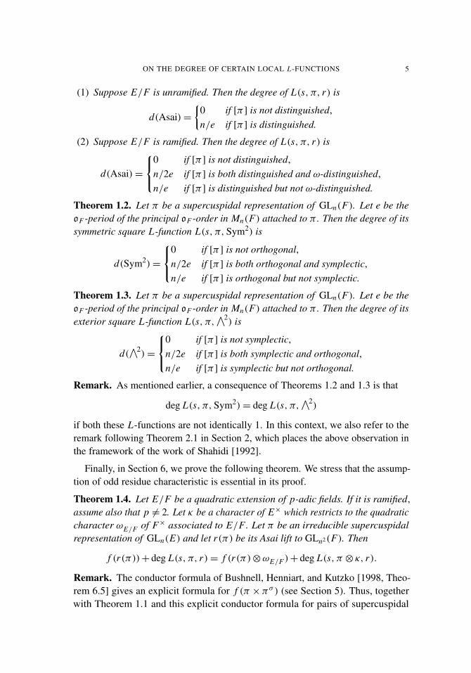
(1) Suppose E/F is unramified. Then the degree of L(s, π, r) is
d(Asai)={
0 if [π ] is not distinguished,n/e if [π ] is distinguished.
(2) Suppose E/F is ramified. Then the degree of L(s, π, r) is
d(Asai)=
0 if [π ] is not distinguished,n/2e if [π ] is both distinguished and ω-distinguished,n/e if [π ] is distinguished but not ω-distinguished.
Theorem 1.2. Let π be a supercuspidal representation of GLn(F). Let e be theoF -period of the principal oF -order in Mn(F) attached to π . Then the degree of itssymmetric square L-function L(s, π,Sym2) is
d(Sym2)=
0 if [π ] is not orthogonal,n/2e if [π ] is both orthogonal and symplectic,n/e if [π ] is orthogonal but not symplectic.
Theorem 1.3. Let π be a supercuspidal representation of GLn(F). Let e be theoF -period of the principal oF -order in Mn(F) attached to π . Then the degree of itsexterior square L-function L(s, π,
∧2) is
d(∧2)=
0 if [π ] is not symplectic,n/2e if [π ] is both symplectic and orthogonal,n/e if [π ] is symplectic but not orthogonal.
Remark. As mentioned earlier, a consequence of Theorems 1.2 and 1.3 is that
deg L(s, π,Sym2)= deg L(s, π,∧2)
if both these L-functions are not identically 1. In this context, we also refer to theremark following Theorem 2.1 in Section 2, which places the above observation inthe framework of the work of Shahidi [1992].
Finally, in Section 6, we prove the following theorem. We stress that the assump-tion of odd residue characteristic is essential in its proof.
Theorem 1.4. Let E/F be a quadratic extension of p-adic fields. If it is ramified,assume also that p 6= 2. Let κ be a character of E× which restricts to the quadraticcharacter ωE/F of F× associated to E/F. Let π be an irreducible supercuspidalrepresentation of GLn(E) and let r(π) be its Asai lift to GLn2(F). Then
f (r(π))+ deg L(s, π, r)= f (r(π)⊗ωE/F )+ deg L(s, π ⊗ κ, r).
Remark. The conductor formula of Bushnell, Henniart, and Kutzko [1998, Theo-rem 6.5] gives an explicit formula for f (π ×πσ ) (see Section 5). Thus, togetherwith Theorem 1.1 and this explicit conductor formula for pairs of supercuspidal
6 U. K. ANANDAVARDHANAN AND AMIYA KUMAR MONDAL
representations of general linear groups, Theorem 1.4 in fact produces an explicitconductor formula for the Asai lift. Since the statement of such an explicit formulainvolves introducing further notations, we leave the precise formula to Section 6(see Theorem 6.1).
2. Results of Shahidi and Goldberg
We recall the results of [Shahidi 1992; Goldberg 1994] to place our Theorems 1.1,1.2, and 1.3 in context. For the unexplained definitions in the following, we refer to[Shahidi 1992, Definitions 7.4 and 7.5].
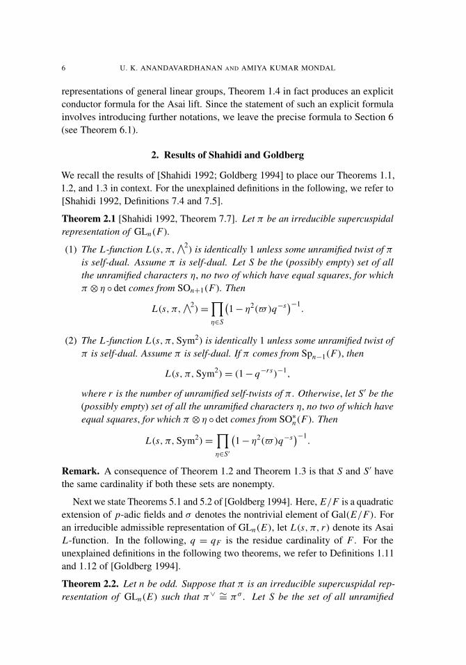
Theorem 2.1 [Shahidi 1992, Theorem 7.7]. Let π be an irreducible supercuspidalrepresentation of GLn(F).
(1) The L-function L(s, π,∧2) is identically 1 unless some unramified twist of π
is self-dual. Assume π is self-dual. Let S be the (possibly empty) set of allthe unramified characters η, no two of which have equal squares, for whichπ ⊗ η ◦ det comes from SOn+1(F). Then
L(s, π,∧2)=
∏η∈S
(1− η2($)q−s)−1
.
(2) The L-function L(s, π,Sym2) is identically 1 unless some unramified twist ofπ is self-dual. Assume π is self-dual. If π comes from Spn−1(F), then
L(s, π,Sym2)= (1− q−rs)−1,
where r is the number of unramified self-twists of π . Otherwise, let S′ be the(possibly empty) set of all the unramified characters η, no two of which haveequal squares, for which π ⊗ η ◦ det comes from SO∗n(F). Then
L(s, π,Sym2)=∏η∈S′
(1− η2($)q−s)−1
.
Remark. A consequence of Theorem 1.2 and Theorem 1.3 is that S and S′ havethe same cardinality if both these sets are nonempty.
Next we state Theorems 5.1 and 5.2 of [Goldberg 1994]. Here, E/F is a quadraticextension of p-adic fields and σ denotes the nontrivial element of Gal(E/F). Foran irreducible admissible representation of GLn(E), let L(s, π, r) denote its AsaiL-function. In the following, q = qF is the residue cardinality of F . For theunexplained definitions in the following two theorems, we refer to Definitions 1.11and 1.12 of [Goldberg 1994].
Theorem 2.2. Let n be odd. Suppose that π is an irreducible supercuspidal rep-resentation of GLn(E) such that π∨ ∼= πσ . Let S be the set of all unramified
ON THE DEGREE OF CERTAIN LOCAL L -FUNCTIONS 7
characters η of E×, no two of which have equal squares, such that π ⊗ η ◦ det is astable lift from U (n, E/F).
(1) Suppose E/F is ramified. Then
L(s, π, r)=∏η∈S
(1− η($F )q
−s)−1.
(2) Suppose E/F is unramified. Then
L(s, π, r)=∏η∈S
(1− η2($F )q
−s)−1.
Theorem 2.3. Let n be even. Suppose that π is an irreducible supercuspidalrepresentation of GLn(E) such that π∨ ∼= πσ . Let S be the set of all unramifiedcharacters η of E×, no two of which have equal value at $F , such that π ⊗ η ◦ detis an unstable lift from U (n, E/F). Then
L(s, π, r)=∏η∈S
(1− η($F )q
−s)−1.
Remark. Theorem 1.1 computes explicitly the cardinality of S in Theorems 2.2and 2.3.
3. The Asai lift
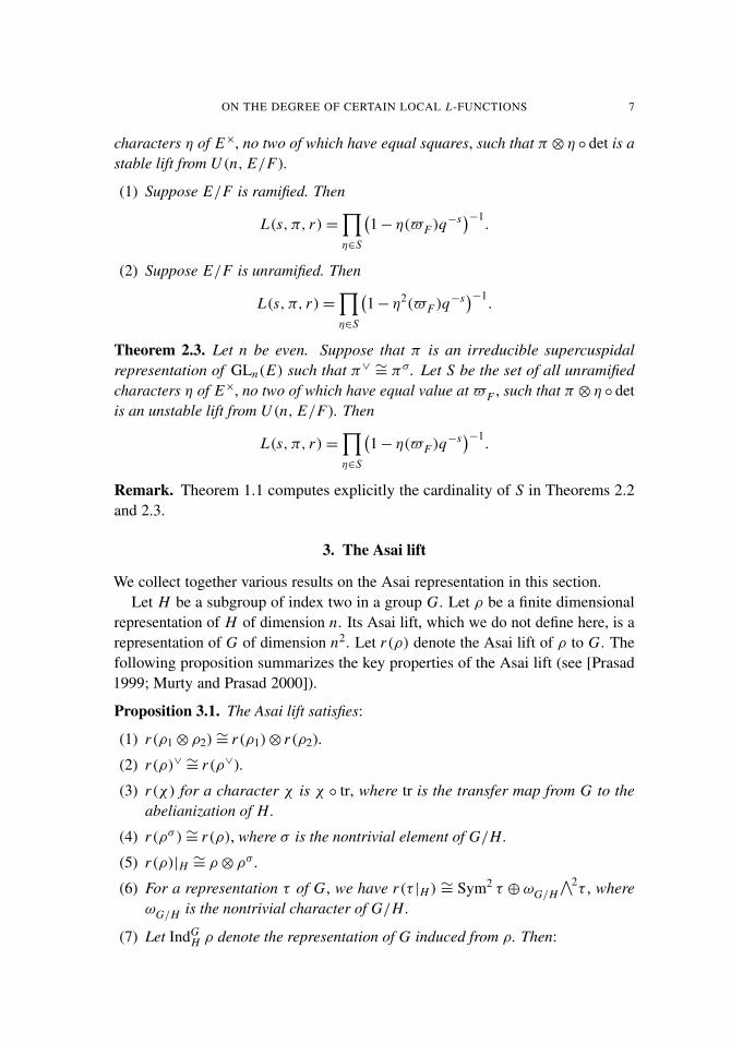
We collect together various results on the Asai representation in this section.Let H be a subgroup of index two in a group G. Let ρ be a finite dimensional
representation of H of dimension n. Its Asai lift, which we do not define here, is arepresentation of G of dimension n2. Let r(ρ) denote the Asai lift of ρ to G. Thefollowing proposition summarizes the key properties of the Asai lift (see [Prasad1999; Murty and Prasad 2000]).
Proposition 3.1. The Asai lift satisfies:
(1) r(ρ1⊗ ρ2)∼= r(ρ1)⊗ r(ρ2).
(2) r(ρ)∨ ∼= r(ρ∨).
(3) r(χ) for a character χ is χ ◦ tr, where tr is the transfer map from G to theabelianization of H.
(4) r(ρσ )∼= r(ρ), where σ is the nontrivial element of G/H.
(5) r(ρ)|H ∼= ρ⊗ ρσ .
(6) For a representation τ of G, we have r(τ |H ) ∼= Sym2 τ ⊕ ωG/H∧2τ , where
ωG/H is the nontrivial character of G/H.
(7) Let IndGH ρ denote the representation of G induced from ρ. Then:

8 U. K. ANANDAVARDHANAN AND AMIYA KUMAR MONDAL
(a) Sym2(IndGH ρ)∼= IndG
H Sym2 ρ⊕ r(ρ).(b)
∧2(IndG
H ρ)∼= IndG
H∧2ρ⊕ r(ρ)⊗ωG/H .
Remark. We have assumed [G : H ] = 2 since that is the case of interest to us. TheAsai lift can be more generally defined when H is of any finite index in G.
4. Proofs of Theorems 1.1–1.3
We now prove Theorems 1.1, 1.2, and 1.3. We first prove (1) of Theorem 1.1, usethis to prove Theorems 1.2 and 1.3, and finally prove (2) of Theorem 1.1. We willappeal to a result mentioned in Section 1, which we formally state now for ease ofreference.
Theorem 4.1 [Bushnell and Kutzko 1993, Lemma 6.2.5]. Let π be an irreduciblesupercuspidal representation of GLn(E). Let [A,m, 0, β] be the simple stratumdefining a maximal simple type occurring in π , where A is a principal oE -orderin Mn(E), m ≥ 0 is the level of π , and β ∈ Mn(E) is such that E[β] is a fieldwith E[β]× normalizing A. Let e = e(A|oE) be the oE -period of A (which is thesame as the ramification index e(E[β]/E) of E[β]/E). Then e divides n, and thecardinality of the group of unramified self-twists of π is n/e.
Proof of Theorem 1.1(1). Let E/F be quadratic unramified. Let π be a supercuspidalrepresentation of GLn(E). Let ρπ :WE→GLn(C) be its Langlands parameter. Weassume that its Asai lift r(ρπ ) :WF→GLn2(C) contains the trivial character of WF ,which in particular implies that ρσπ ∼= ρ
∨π . Since ω = ωE/F is unramified, clearly
the number of unramified characters in r(ρπ ) and r(ρπ )⊗ω is the same. Since
deg L(s, π, r)+ deg L(s, π ⊗ κ, r)= deg L(s, π ×π∨)= 2n/e
by Theorem 4.1, item (1) of Theorem 1.1 is immediate. �
Proof of Theorems 1.2 and 1.3. Let π be a supercuspidal representation of GLn(F).Let ρπ :WF→GLn(C) be its Langlands parameter. We assume that r(ρπ ) containsthe trivial character of WF , which in particular implies that ρπ ∼= ρ∨π . Here, r iseither the symmetric square representation or the exterior square representation ofGLn(C). Thus, the dimension of r(ρπ ) is either n(n+1)/2 or n(n−1)/2. We havethe identity
L(s, π ×π)= L(s, π,Sym2)L(s, π,∧2),
and we know that the left-hand side L-function has degree n/e by Theorem 4.1.If n/e = 1, then the trivial character of WF is the only unramified character
appearing in ρπ ⊗ ρ∨π and hence in r(ρπ ). Therefore, in this case there is nothingto prove. Otherwise, there is a nontrivial unramified character χ :WF → C× suchthat ρπ ⊗χ ∼= ρπ . Thus,
ρπ = IndWFWF ′
τ
ON THE DEGREE OF CERTAIN LOCAL L -FUNCTIONS 9
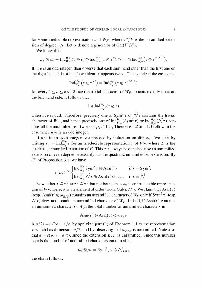
for some irreducible representation τ of WF ′ , where F ′/F is the unramified exten-sion of degree n/e. Let σ denote a generator of Gal(F ′/F).
We know that
ρπ ⊗ ρπ = IndWFWF ′(τ ⊗ τ)⊕ IndWF
WF ′(τ ⊗ τ σ )⊕ · · ·⊕ IndWF
WF ′
(τ ⊗ τ σ
n/e−1).
If n/e is an odd integer, then observe that each summand other than the first one onthe right-hand side of the above identity appears twice. This is indeed the case since
IndWFWF ′
(τ ⊗ τ σ
a)= IndWF
WF ′
(τ ⊗ τ σ
n/e−a)for every 1≤ a ≤ n/e. Since the trivial character of WF appears exactly once onthe left-hand side, it follows that
1 ∈ IndWFWF ′(τ ⊗ τ)
when n/e is odd. Therefore, precisely one of Sym2 τ or∧2τ contains the trivial
character of WF ′ , and hence precisely one of IndWFWF ′(Sym2 τ) or IndWF
WF ′(∧2τ) con-
tains all the unramified self-twists of ρπ . Thus, Theorems 1.2 and 1.3 follow in thecase when n/e is an odd integer.
If n/e is an even integer, we proceed by induction on dim ρπ . We start bywriting ρπ = IndWF
WEτ for an irreducible representation τ of WE , where E is the
quadratic unramified extension of F . This can always be done because an unramifiedextension of even degree necessarily has the quadratic unramified subextension. By(7) of Proposition 3.1, we have
r(ρπ )∼=
{IndWF
WESym2 τ ⊕Asai(τ ) if r = Sym2,
IndWFWE
∧2τ ⊕Asai(τ )⊗ωE/F if r =
∧2.
Now either τ ∼= τ∨ or τ σ ∼= τ∨ but not both, since ρπ is an irreducible representa-tion of WF . Here, σ is the element of order two in Gal(E/F). We claim that Asai(τ )(resp. Asai(τ )⊗ωE/F ) contains an unramified character of WF only if Sym2 τ (resp.∧2τ ) does not contain an unramified character of WF . Indeed, if Asai(τ ) contains
an unramified character of WF , the total number of unramified characters in
Asai(τ )⊕Asai(τ )⊗ωE/F
is n/2e+ n/2e = n/e, by applying part (1) of Theorem 1.1 to the representationτ which has dimension n/2, and by observing that ωE/F is unramified. Note alsothat e = e(ρπ )= e(τ ), since the extension E/F is unramified. Since this numberequals the number of unramified characters contained in
ρπ ⊗ ρπ = Sym2 ρπ ⊕∧2ρπ ,
the claim follows.
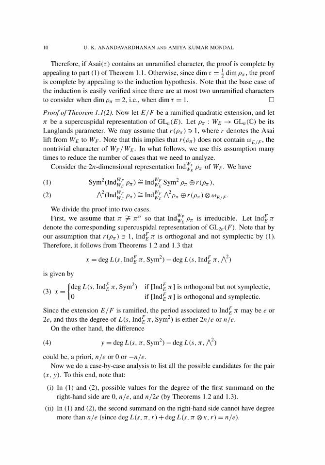
10 U. K. ANANDAVARDHANAN AND AMIYA KUMAR MONDAL
Therefore, if Asai(τ ) contains an unramified character, the proof is complete byappealing to part (1) of Theorem 1.1. Otherwise, since dim τ = 1
2 dim ρπ , the proofis complete by appealing to the induction hypothesis. Note that the base case ofthe induction is easily verified since there are at most two unramified charactersto consider when dim ρπ = 2, i.e., when dim τ = 1. �
Proof of Theorem 1.1(2). Now let E/F be a ramified quadratic extension, and letπ be a supercuspidal representation of GLn(E). Let ρπ : WE → GLn(C) be itsLanglands parameter. We may assume that r(ρπ ) 3 1, where r denotes the Asailift from WE to WF . Note that this implies that r(ρπ ) does not contain ωE/F , thenontrivial character of WF/WE . In what follows, we use this assumption manytimes to reduce the number of cases that we need to analyze.
Consider the 2n-dimensional representation IndWFWEρπ of WF . We have
Sym2(IndWFWEρπ )∼= IndWF
WESym2 ρπ ⊕ r(ρπ ),(1) ∧2
(IndWFWEρπ )∼= IndWF
WE
∧2ρπ ⊕ r(ρπ )⊗ωE/F .(2)
We divide the proof into two cases.First, we assume that π 6∼= πσ so that IndWF
WEρπ is irreducible. Let IndF
E π
denote the corresponding supercuspidal representation of GL2n(F). Note that byour assumption that r(ρπ ) 3 1, IndF
E π is orthogonal and not symplectic by (1).Therefore, it follows from Theorems 1.2 and 1.3 that
x = deg L(s, IndFE π,Sym2)− deg L(s, IndF
E π,∧2)
is given by
(3) x ={
deg L(s, IndFE π,Sym2) if [IndF
E π ] is orthogonal but not symplectic,0 if [IndF
E π ] is orthogonal and symplectic.
Since the extension E/F is ramified, the period associated to IndFE π may be e or
2e, and thus the degree of L(s, IndFE π,Sym2) is either 2n/e or n/e.
On the other hand, the difference
(4) y = deg L(s, π,Sym2)− deg L(s, π,∧2)
could be, a priori, n/e or 0 or −n/e.Now we do a case-by-case analysis to list all the possible candidates for the pair
(x, y). To this end, note that:
(i) In (1) and (2), possible values for the degree of the first summand on theright-hand side are 0, n/e, and n/2e (by Theorems 1.2 and 1.3).
(ii) In (1) and (2), the second summand on the right-hand side cannot have degreemore than n/e (since deg L(s, π, r)+ deg L(s, π ⊗ κ, r)= n/e).
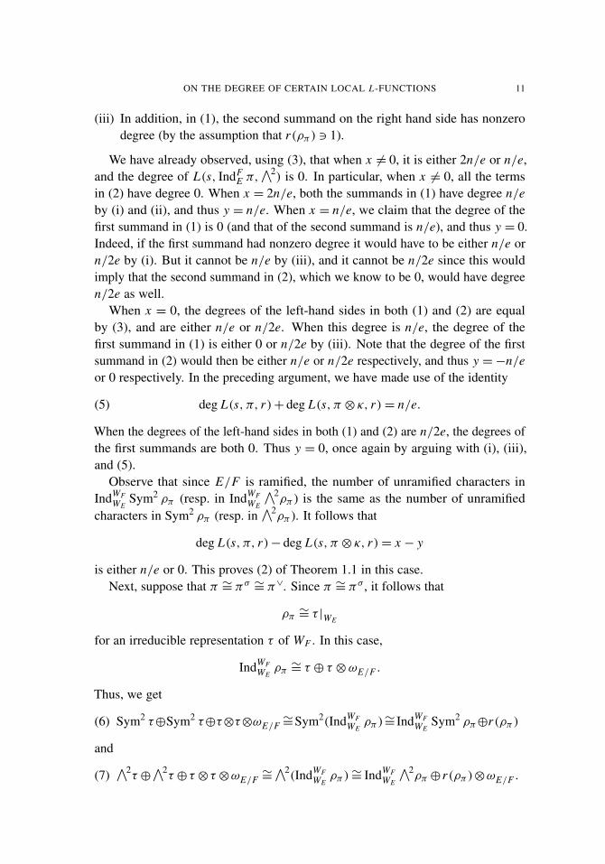
ON THE DEGREE OF CERTAIN LOCAL L -FUNCTIONS 11
(iii) In addition, in (1), the second summand on the right hand side has nonzerodegree (by the assumption that r(ρπ ) 3 1).
We have already observed, using (3), that when x 6= 0, it is either 2n/e or n/e,and the degree of L(s, IndF
E π,∧2) is 0. In particular, when x 6= 0, all the terms
in (2) have degree 0. When x = 2n/e, both the summands in (1) have degree n/eby (i) and (ii), and thus y = n/e. When x = n/e, we claim that the degree of thefirst summand in (1) is 0 (and that of the second summand is n/e), and thus y = 0.Indeed, if the first summand had nonzero degree it would have to be either n/e orn/2e by (i). But it cannot be n/e by (iii), and it cannot be n/2e since this wouldimply that the second summand in (2), which we know to be 0, would have degreen/2e as well.
When x = 0, the degrees of the left-hand sides in both (1) and (2) are equalby (3), and are either n/e or n/2e. When this degree is n/e, the degree of thefirst summand in (1) is either 0 or n/2e by (iii). Note that the degree of the firstsummand in (2) would then be either n/e or n/2e respectively, and thus y =−n/eor 0 respectively. In the preceding argument, we have made use of the identity
(5) deg L(s, π, r)+ deg L(s, π ⊗ κ, r)= n/e.
When the degrees of the left-hand sides in both (1) and (2) are n/2e, the degrees ofthe first summands are both 0. Thus y = 0, once again by arguing with (i), (iii),and (5).
Observe that since E/F is ramified, the number of unramified characters inIndWF
WESym2 ρπ (resp. in IndWF
WE
∧2ρπ ) is the same as the number of unramified
characters in Sym2 ρπ (resp. in∧2ρπ ). It follows that
deg L(s, π, r)− deg L(s, π ⊗ κ, r)= x − y
is either n/e or 0. This proves (2) of Theorem 1.1 in this case.Next, suppose that π ∼= πσ ∼= π∨. Since π ∼= πσ , it follows that
ρπ ∼= τ |WE
for an irreducible representation τ of WF . In this case,
IndWFWEρπ ∼= τ ⊕ τ ⊗ωE/F .
Thus, we get
(6) Sym2 τ⊕Sym2 τ⊕τ⊗τ⊗ωE/F∼=Sym2(IndWF
WEρπ )∼= IndWF
WESym2 ρπ⊕r(ρπ )
and
(7)∧2τ ⊕
∧2τ ⊕τ ⊗τ ⊗ωE/F
∼=∧2(IndWF
WEρπ )∼= IndWF
WE
∧2ρπ ⊕r(ρπ )⊗ωE/F .
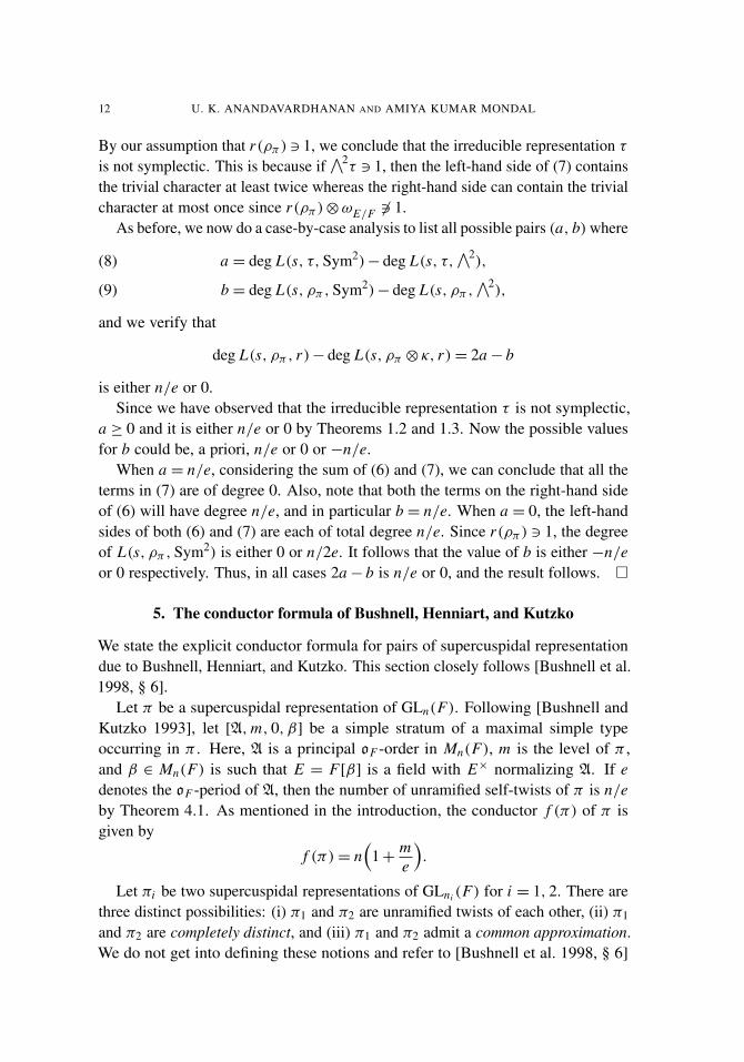
12 U. K. ANANDAVARDHANAN AND AMIYA KUMAR MONDAL
By our assumption that r(ρπ ) 3 1, we conclude that the irreducible representation τis not symplectic. This is because if
∧2τ 3 1, then the left-hand side of (7) contains
the trivial character at least twice whereas the right-hand side can contain the trivialcharacter at most once since r(ρπ )⊗ωE/F 63 1.
As before, we now do a case-by-case analysis to list all possible pairs (a, b)where
a = deg L(s, τ,Sym2)− deg L(s, τ,∧2),(8)
b = deg L(s, ρπ ,Sym2)− deg L(s, ρπ ,∧2),(9)
and we verify that
deg L(s, ρπ , r)− deg L(s, ρπ ⊗ κ, r)= 2a− b
is either n/e or 0.Since we have observed that the irreducible representation τ is not symplectic,
a ≥ 0 and it is either n/e or 0 by Theorems 1.2 and 1.3. Now the possible valuesfor b could be, a priori, n/e or 0 or −n/e.
When a = n/e, considering the sum of (6) and (7), we can conclude that all theterms in (7) are of degree 0. Also, note that both the terms on the right-hand sideof (6) will have degree n/e, and in particular b = n/e. When a = 0, the left-handsides of both (6) and (7) are each of total degree n/e. Since r(ρπ ) 3 1, the degreeof L(s, ρπ ,Sym2) is either 0 or n/2e. It follows that the value of b is either −n/eor 0 respectively. Thus, in all cases 2a− b is n/e or 0, and the result follows. �
5. The conductor formula of Bushnell, Henniart, and Kutzko
We state the explicit conductor formula for pairs of supercuspidal representationdue to Bushnell, Henniart, and Kutzko. This section closely follows [Bushnell et al.1998, § 6].
Let π be a supercuspidal representation of GLn(F). Following [Bushnell andKutzko 1993], let [A,m, 0, β] be a simple stratum of a maximal simple typeoccurring in π . Here, A is a principal oF -order in Mn(F), m is the level of π ,and β ∈ Mn(F) is such that E = F[β] is a field with E× normalizing A. If edenotes the oF -period of A, then the number of unramified self-twists of π is n/eby Theorem 4.1. As mentioned in the introduction, the conductor f (π) of π isgiven by
f (π)= n(
1+ me
).
Let πi be two supercuspidal representations of GLni (F) for i = 1, 2. There arethree distinct possibilities: (i) π1 and π2 are unramified twists of each other, (ii) π1
and π2 are completely distinct, and (iii) π1 and π2 admit a common approximation.We do not get into defining these notions and refer to [Bushnell et al. 1998, § 6]

ON THE DEGREE OF CERTAIN LOCAL L -FUNCTIONS 13
instead. Suffice to say that when π1 and π2 admit a common approximation, there isa best common approximation and this is an object of the form ([3,m, 0, γ ], l, ϑ),where the stratum [3,m, 0, γ ] is determined by π1 and π2, 0≤ l <m is an integer,and ϑ is a character of a compact group attached to the data coming from π1 and π2.
Another ingredient in the conductor formula is an integer c(β) associated toβ. This comes from the “generalized discriminant”, say C(β), associated to theexact sequence
0−→ E −→ EndF (E)aβ−→EndF (E)
sβ−→ E −→ 0,
where sβ is a tame corestriction relative to E/F [Bushnell and Kutzko 1993, § 1.3]and aβ is the adjoint map x 7→ βx − xβ. The constant c(β) is defined such that
C(β)= qc(β).
Now we state the conductor formula of [Bushnell et al. 1998].
Theorem 5.1 (Bushnell, Henniart, and Kutzko). For i=1, 2, let πi be an irreduciblesupercuspidal representation of GLni (F). Define quantities mi , ei , βi as above. Lete = lcm(e1, e2) and m/e =max{m1/e1,m2/e2}.
(1) Suppose that n1 = n2 = n and π1 and π2 are unramified twists of each other.Let β = β1 and d = [F[β] : F]. Then
f (π∨1 ×π2)= n2(
1+c(β)
d2
)− deg L(s, π∨1 ×π2).
(2) Suppose that π1 and π2 are completely distinct. Then
f (π∨1 ×π2)= n1n2
(1+ m
e
).
(3) Suppose that π2 is not equivalent to an unramified twist of π1, but that π1
and π2 are not completely distinct. Let ([3,m, 0, γ ], l, ϑ) be a best commonapproximation to the πi , and assume that the stratum [3,m, l, γ ] is simple.Put d = [F[γ ] : F]. Then
f (π∨1 ×π2)= n1n2
(1+
c(γ )
d2 +l
de
).
Remark. Observe that in (2) and (3), deg L(s, π∨1 ×π2)= 0.
6. Conductor of the Asai lift
Let E/F be a quadratic extension of p-adic fields. Let π be a supercuspidalrepresentation of GLn(E). Let ρπ : WE → GLn(C) be its Langlands parameter.Let r(ρπ ) :WF → GLn2(C) be the Asai lift of ρπ . In this section, we compute the
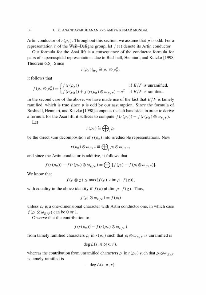
14 U. K. ANANDAVARDHANAN AND AMIYA KUMAR MONDAL
Artin conductor of r(ρπ ). Throughout this section, we assume that p is odd. For arepresentation τ of the Weil–Deligne group, let f (τ ) denote its Artin conductor.
Our formula for the Asai lift is a consequence of the conductor formula forpairs of supercuspidal representations due to Bushnell, Henniart, and Kutzko [1998,Theorem 6.5]. Since
r(ρπ )|WE∼= ρπ ⊗ ρ
σπ ,
it follows that
f (ρπ ⊗ ρσπ )={
f (r(ρπ )) if E/F is unramified,f (r(ρπ ))+ f (r(ρπ )⊗ωE/F )− n2 if E/F is ramified.
In the second case of the above, we have made use of the fact that E/F is tamelyramified, which is true since p is odd by our assumption. Since the formula ofBushnell, Henniart, and Kutzko [1998] computes the left hand side, in order to derivea formula for the Asai lift, it suffices to compute f (r(ρπ ))− f (r(ρπ )⊗ωE/F ).
Letr(ρπ )∼=
⊕iρi
be the direct sum decomposition of r(ρπ ) into irreducible representations. Now
r(ρπ )⊗ωE/F∼=
⊕iρi ⊗ωE/F ,
and since the Artin conductor is additive, it follows that
f (r(ρπ ))− f (r(ρπ )⊗ωE/F )=⊕
i[ f (ρi )− f (ρi ⊗ωE/F )].
We know thatf (ρ⊗χ)≤max{ f (ρ), dim ρ · f (χ)},
with equality in the above identity if f (ρ) 6= dim ρ · f (χ). Thus,
f (ρi ⊗ωE/F )= f (ρi )
unless ρi is a one-dimensional character with Artin conductor one, in which casef (ρi ⊗ωE/F ) can be 0 or 1.
Observe that the contribution to
f (r(ρπ ))− f (r(ρπ )⊗ωE/F )
from tamely ramified characters ρi in r(ρπ ) such that ρi ⊗ωE/F is unramified is
deg L(s, π ⊗ κ, r),
whereas the contribution from unramified characters ρi in r(ρπ ) such that ρi⊗ωE/Fis tamely ramified is
− deg L(s, π, r).

ON THE DEGREE OF CERTAIN LOCAL L -FUNCTIONS 15
Therefore, it follows that
f (r(ρπ ))− f (r(ρπ )⊗ωE/F )= deg L(s, π ⊗ κ, r)− deg L(s, π, r).
Now making use of Theorem 5.1, we get the following conductor formula forthe Asai lift.
Theorem 6.1. Let E/F be a quadratic extension of p-adic fields, where p is odd,with ramification index e(E/F). Let σ denote the nontrivial element of Gal(E/F).Let π be a supercuspidal representation of GLn(E). Let e be the oE -period of theprincipal oE -order in Mn(E) attached to π . Let r(π) be its Asai lift to GLn2(F)and let L(s, π, r) be the Asai L-function attached to π .
(1) Suppose π∨ and πσ are unramified twists of each other. Then
f (r(π))= n2(
1+c(β)
e(E/F)d2
)− deg L(s, π, r).
(2) Suppose π∨ and πσ are completely distinct. Then
f (r(π))= n2(
1+m
e(E/F)e
).
(3) Suppose that π∨ is not equivalent to an unramified twist of πσ and thatthey are not completely distinct. Let ([3,m, 0, γ ], l, ϑ) be a best commonapproximation to π∨ and πσ , and assume that the stratum [3,m, l, γ ] issimple. Set d = [F[γ ] : F]. Then
f (r(π))= n2(
1+c(γ )
e(E/F)d2 +l
e(E/F)de
).
Remark. Together with Theorem 1.1, Theorem 6.1 gives an explicit conductorformula for the Asai lift. As in the case of Theorem 5.1, deg L(s, π, r)= 0 in cases(2) and (3).
Acknowledgements
The authors thank Dipendra Prasad for several useful discussions. They thank theanonymous referee for carefully reading the manuscript and for making severaluseful suggestions. The second named author would like to acknowledge a grant(07IR001) from the Industrial Research and Consultancy Centre, Indian Institute ofTechnology Bombay, during the period of the present work.
References
[Anandavardhanan and Rajan 2005] U. K. Anandavardhanan and C. S. Rajan, “Distinguished repre-sentations, base change, and reducibility for unitary groups”, Int. Math. Res. Not. 2005:14 (2005),841–854. MR 2006g:22013 Zbl 1070.22011

16 U. K. ANANDAVARDHANAN AND AMIYA KUMAR MONDAL
[Anandavardhanan et al. 2004] U. K. Anandavardhanan, A. C. Kable, and R. Tandon, “Distinguishedrepresentations and poles of twisted tensor L-functions”, Proc. Amer. Math. Soc. 132:10 (2004),2875–2883. MR 2005g:11080 Zbl 1122.11033
[Bump and Ginzburg 1992] D. Bump and D. Ginzburg, “Symmetric square L-functions on GL(r)”,Ann. of Math. (2) 136:1 (1992), 137–205. MR 93i:11058 Zbl 0753.11021
[Bushnell and Kutzko 1993] C. J. Bushnell and P. C. Kutzko, The admissible dual of GL(N ) viacompact open subgroups, Annals of Mathematics Studies 129, Princeton University Press, 1993.MR 94h:22007 Zbl 0787.22016
[Bushnell et al. 1998] C. J. Bushnell, G. M. Henniart, and P. C. Kutzko, “Local Rankin–Selbergconvolutions for GLn : explicit conductor formula”, J. Amer. Math. Soc. 11:3 (1998), 703–730.MR 99h:22022 Zbl 0899.22017
[Flicker 1993] Y. Z. Flicker, “On zeroes of the twisted tensor L-function”, Math. Ann. 297:2 (1993),199–219. MR 95c:11065 Zbl 0786.11030
[Goldberg 1994] D. Goldberg, “Some results on reducibility for unitary groups and local AsaiL-functions”, J. Reine Angew. Math. 448 (1994), 65–95. MR 95g:22031 Zbl 0815.11029
[Henniart 2010] G. M. Henniart, “Correspondance de Langlands et fonctions L des carrés extérieuret symétrique”, Int. Math. Res. Not. 2010:4 (2010), 633–673. MR 2011c:22028 Zbl 1184.22009
[Jacquet and Shalika 1990] H. Jacquet and J. A. Shalika, “Exterior square L-functions”, pp. 143–226in Automorphic forms, Shimura varieties, and L-functions (Ann Arbor, MI, 1988), vol. 2, editedby L. Clozel and J. S. Milne, Perspectives in Mathematics 11, Academic Press, Boston, 1990.MR 91g:11050 Zbl 0695.10025
[Jacquet et al. 1983] H. Jacquet, I. I. Piatetskii-Shapiro, and J. A. Shalika, “Rankin–Selberg convolu-tions”, Amer. J. Math. 105:2 (1983), 367–464. MR 85g:11044 Zbl 0525.22018
[Jiang et al. 2008] D. Jiang, C. Nien, and Y. Qin, “Local Shalika models and functoriality”, Manu-scripta Math. 127:2 (2008), 187–217. MR 2010b:11057 Zbl 1167.11021
[Kable 2004] A. C. Kable, “Asai L-functions and Jacquet’s conjecture”, Amer. J. Math. 126:4 (2004),789–820. MR 2005g:11083 Zbl 1061.11023
[Kewat and Raghunathan 2012] P. K. Kewat and R. Raghunathan, “On the local and global exteriorsquare L-functions of GLn”, Math. Res. Lett. 19:4 (2012), 785–804. MR 3008415 Zbl 06165853
[Matringe 2011] N. Matringe, “Distinguished generic representations of GL(n) over p-adic fields”,Int. Math. Res. Not. 2011:1 (2011), 74–95. MR 2012f:22032 Zbl 1223.22015
[Murty and Prasad 2000] V. K. Murty and D. Prasad, “Tate cycles on a product of two Hilbert modularsurfaces”, J. Number Theory 80:1 (2000), 25–43. MR 2000m:14028 Zbl 0955.14016
[Prasad 1999] D. Prasad, “Some remarks on representations of a division algebra and of the Galoisgroup of a local field”, J. Number Theory 74:1 (1999), 73–97. MR 99m:11138 Zbl 0931.11054
[Shahidi 1984] F. Shahidi, “Fourier transforms of intertwining operators and Plancherel measures forGL(n)”, Amer. J. Math. 106:1 (1984), 67–111. MR 86b:22031 Zbl 0567.22008
[Shahidi 1990] F. Shahidi, “A proof of Langlands’ conjecture on Plancherel measures; complementaryseries for p-adic groups”, Ann. of Math. (2) 132:2 (1990), 273–330. MR 91m:11095 Zbl 0780.22005
[Shahidi 1992] F. Shahidi, “Twisted endoscopy and reducibility of induced representations for p-adicgroups”, Duke Math. J. 66:1 (1992), 1–41. MR 93b:22034 Zbl 0785.22022
Received March 31, 2014. Revised November 9, 2014.
ON THE DEGREE OF CERTAIN LOCAL L -FUNCTIONS 17
U. K. ANANDAVARDHANAN
DEPARTMENT OF MATHEMATICS
INDIAN INSTITUTE OF TECHNOLOGY BOMBAY
MUMBAI 400076INDIA
AMIYA KUMAR MONDAL
DEPARTMENT OF MATHEMATICS
INDIAN INSTITUTE OF TECHNOLOGY BOMBAY
MUMBAI 400076INDIA

PACIFIC JOURNAL OF MATHEMATICSVol. 276, No. 1, 2015
dx.doi.org/10.2140/pjm.2015.276.19
TORUS ACTIONS AND TENSOR PRODUCTSOF INTERSECTION COHOMOLOGY
ASILATA BAPAT
Given certain intersection cohomology sheaves on a projective variety witha torus action, we relate the cohomology groups of their tensor product tothe cohomology groups of the individual sheaves. We also prove a similarresult in the case of equivariant cohomology.
1. Introduction
Let X be a smooth complex projective variety together with an action of a complexalgebraic torus T with isolated fixed points. We fix a regular algebraic one-parametersubgroup λ : C∗→ T, which means that the set of λ-fixed points on X equals the setof T-fixed points on X (denoted X T ). Consider the Białynicki-Birula decomposition[1973] of X : for each w ∈ X T define the plus and minus cells to be respectively
Uw =U+w = {x ∈ X | limt→0
λ(t) · x = w}, t ∈ C∗, and
U−w = {x ∈ X | limt→∞
λ(t) · x = w}, t ∈ C∗.
Each plus or minus cell is a λ-stable affine space, and hence the decompositionsX =
∐w∈X T Uw and X =
∐w∈X T U−w are cell decompositions. For the purposes of
this paper, we make the following additional assumptions on the T-action on X .
Assumption 1.1. The cell decompositions X =∐w∈X T Uw and X =
∐w∈X T U−w
are algebraic stratifications of X . In particular, the closure of every plus cell is aunion of plus cells, and analogously for minus cells.
Assumption 1.2. For eachw∈ X T, there is a one-parameter subgroup λw : C∗→ Tand a neighborhood Vw of w such that limt→0 λw(t) · v = w for every v ∈ Vw andt ∈ C∗.
In this paper, we use the words sheaf and complex of sheaves interchangeablyto mean an object in Db
c,BB(X,C), the bounded derived category of sheaves ofC-vector spaces on X that are constructible with respect to the Białynicki-Birula
MSC2010: 14F05, 14F43, 14L30, 55N33.Keywords: intersection cohomology, torus action.
19
20 ASILATA BAPAT
stratification. (Here we make use of Assumption 1.1.) Moreover all functors arederived, so for ease of notation we omit the decorations R and L.
For each w ∈ X T, let ICw denote the intersection cohomology sheaf on theclosure of the cell Uw, extended by zero to all of X . The main theorem of the paperdescribes the cohomology of the tensor products of a collection of ICw, in terms ofthe tensor products of the cohomologies of the individual ICw.
Main result. Let 1 : X→ Xm be the diagonal embedding. Consider any sheavesF1, . . . ,Fm in Db
c,BB(X,C). Then their (derived) tensor product is also a sheaf inDb
c,BB(X,C), and will be denoted by F1⊗ · · ·⊗Fm . Recall that
F1⊗ · · ·⊗Fm =1−1(F1 � · · ·�Fm).
For any sheaf F, its cohomology H •(F) = H •(X,F) is a graded vector space.There is a natural cup product ∪: H •(F1)⊗· · ·⊗ H •(Fm)→ H •(F1⊗ · · ·⊗Fm),defined on page 22.
Let C denote the constant sheaf on X . For any sheaf F, its cohomology H •(F) isnaturally a (graded) left and right module over the (graded) ring H(X)= H •(X,C),as follows:
∪: H(X)⊗ H •(F)→ H •(C⊗F)−→∼= H •(F),
∪: H •(F)⊗ H(X)→ H •(F⊗C)−→∼= H •(F).
Moreover, the cup product descends to a morphism
H •(F1) ⊗H(X)· · · ⊗
H(X)H •(Fm)→ H •(F1⊗ · · ·⊗Fm).
Theorem 1.3. Let (p1, . . . , pm) be an m-tuple of T-fixed points of X , and supposethat Assumptions 1.1 and 1.2 hold. Then the cup product map
(1-1) H •(ICp1) ⊗H(X)· · · ⊗
H(X)H •(ICpm )→ H •(ICp1 ⊗ · · ·⊗ ICpm )
is an isomorphism.
As X is a T-space, each IC sheaf ICp j carries a canonical T-equivariant structure,and so does the tensor product ICp1 ⊗ · · · ⊗ ICpm . Let HT (X) = H •
T (X,C) bethe T-equivariant cohomology of X . For any T-equivariant sheaf F on X , itsT-equivariant cohomology H •
T (F) = H •
T (X,F) is a graded HT (X)-module. Asbefore, there is a cup product map for T-equivariant cohomology, which factorsthrough HT (X).
Theorem 1.4. Under Assumptions 1.1 and 1.2, the cup product map
H •
T (ICp1) ⊗HT (X)
· · · ⊗HT (X)
H •
T (ICpm )→ H •
T (ICp1 ⊗ · · ·⊗ ICpm )
is an isomorphism.

TORUS ACTIONS AND TENSOR PRODUCTS OF INTERSECTION COHOMOLOGY 21
Remark 1.5. Even though our results are stated using IC sheaves, it is possible thatthey generalize to parity sheaves (defined and discussed by Juteau, Mautner, andWilliamson in [Juteau et al. 2014]). Our results and proof methods are similar to themain theorem from [Ginzburg 1991]. Achar and Rider [2014, Theorem 4.1] provea version of Ginzburg’s theorem for parity sheaves on generalized flag varieties ofa Kac–Moody group. Similar generalizations may work in our case as well.
2. Setup
The Białynicki-Birula stratification. One can find (see, e.g., [Sumihiro 1974] or[Kambayashi 1966]) a T-equivariant projective embedding of X into some PN, suchthat the action of T on PN is linear. Consider the following standard Morse–Bottfunction on PN :
[z0 : · · · : zN ] 7→
∑Ni=0 ci |zi |
2∑Ni=0|zi |
2,
where ci are the weights of the λ-action on PN. The critical sets of this functionare precisely the T-fixed points on PN. The Morse–Bott cells of this function arelocally closed algebraic subvarieties of PN. Since X has isolated T-fixed points, onecan show that the composition f : X→ PN
→ R is a Morse function with criticalset X T (see, e.g., [Audin 2004]). Each cell of the Morse decomposition under fis a preimage of a Morse–Bott cell of PN. Hence it is a locally closed algebraicsubvariety of X . Moreover, each cell of the Morse decomposition is known to be aunion of Białynicki-Birula plus cells. A discussion of this may also be found in[Chriss and Ginzburg 1997, Section 2.4].
The collection of fixed points of the λ-action carries a partial order, wherev < w if Uv ⊂ Uw. By the previous discussion, we see that v < w if and only iff (v) < f (w). Fix a weakly increasing enumeration {0, 1, . . . , N } of the points ofX T (sometimes denoted {w0, . . . , wN }), and set Xn =
⋃i≤n Ui . Since the closure
of every plus cell is a union of plus cells, it follows from the previous discussionthat each Xn is a closed subvariety of X .
Similarly, set X−n =⋃
i≥n U−i . By using the Morse function (− f ) instead of f ,we see that each X−n is a closed subvariety of X . Hence we obtain two increasingfiltrations of X by closed subvarieties: X0⊂· · ·⊂ X N = X and X−N ⊂· · ·⊂ X−0 = X .
We have the following inclusions:
Xnin↪→ X, Xn−1
v↪→ Xn
u←↩Un.
For any point p ∈ X−n , we have f (wn) ≤ f (p), with equality only if p ∈ X T.For any point p ∈ Xn , we have f (p)≤ f (wn), with equality only if p ∈ X T. Henceif p ∈ X−n ∩ Xn , then f (p)= f (wn), and p ∈ X T. But X−n ∩ Xn ∩ X T
= {wn}, and
22 ASILATA BAPAT
it follows that p = wn . Hence for every n, the subvarieties X−n and Xn intersecttransversally in the single point wn .
Let cn ∈ H •(X) be the Poincaré dual to the homology class of X−n . As avector space, H •(X) is generated by the collection {cn}. Finally, fix an m-tuple(p1, . . . , pm) of T-fixed points of X , and set L j,n = i−1
n ICp j for each j and n.
The cup product in cohomology. Let π : X → pt be the unique morphism to apoint. For any sheaf F on X , its cohomology H •(F) is a graded vector space, andmay be thought of as π∗F. We use this to define the cup product map.
Recall that the functors (π−1, π∗) form an adjoint pair, which has a counitπ−1◦ π∗ → id. Let F1, . . . ,Fm be sheaves on X . Tensoring the counit maps
together, we have a map
π−1◦π∗(F1)⊗ · · ·⊗π
−1◦π∗(Fm)→ F1⊗ · · ·⊗Fm .
The left hand side is canonically isomorphic to π−1(π∗F1⊗ · · ·⊗π∗Fm). Usingthe (π−1, π∗) adjunction once more, we obtain the cup product:
∪: π∗F1⊗ · · ·⊗π∗Fm→ π∗(F1⊗ · · ·⊗Fm).
The cup product gives each H •(Fi ) the structure of a left and right moduleover H(X). This module structure induces the following map, also called the cupproduct:
H •(F1) ⊗H(X)· · · ⊗
H(X)H •(Fm)→ H •(F1⊗ · · ·⊗Fm).
Proposition 2.1. For every n, the cup product map
(2-1) H •(L1,n) ⊗H(X)· · · ⊗
H(X)H •(Lm,n)→ H •(L1,n ⊗ · · ·⊗ Lm,n)
is an isomorphism.
When Xn = X , we have L j,n = ICp j for each j . Hence Theorem 1.3 followsfrom this proposition, and we now focus on proving the proposition.
3. Proof of the isomorphism
We prove Proposition 2.1 by induction on the nth filtered piece of X0 ⊂ · · · ⊂ X N .In the base case of n = 0, the space X0 is zero-dimensional. Hence each sheaf L j,0
is isomorphic to its cohomology. In this case the cup product map (2-1) reduces tothe identity map, which is an isomorphism.

TORUS ACTIONS AND TENSOR PRODUCTS OF INTERSECTION COHOMOLOGY 23
Now we prove the induction step on the filtered piece Xn . We mainly use thefollowing distinguished triangles:
u!u−1L j,n→ L j,n→ v∗v−1L j,n,(3-1)
v!v!L j,n→ L j,n→ u∗u−1L j,n.(3-2)
After taking cohomology, each of the above distinguished triangles produces along exact sequence. In our case, all connecting homomorphisms of these longexact sequences vanish (see, e.g., [Soergel 1990, Lemma 20] and [Ginzburg 1991,Proposition 3.2]).
For brevity, we will use the following notation through the remainder of thepaper.
(3-3)
Mm,n = L2,n ⊗ · · ·⊗ Lm,n,
Am,n = H •(L2,n) ⊗H(X)· · · ⊗
H(X)H •(Lm,n),
Bm,n = H •(u∗u−1L2,n) ⊗H(X)· · · ⊗
H(X)H •(u∗u−1Lm,n).
The following two lemmas prove the proposition on the open part Un in Xn .
Lemma 3.1. Let F and G be any complexes of sheaves on Un with locally constantcohomology sheaves. Then the cup product map
∪: H •(u!F)⊗ H •(u∗ G)→ H •(u!F⊗ u∗ G)
is an isomorphism. Since ∪ factors through the surjection
H •(u!F)⊗ H •(u∗ G)� H •(u!F) ⊗H(X)
H •(u∗ G),
the induced cup product
∪: H •(u!F) ⊗H(X)
H •(u∗ G)→ H •(u!F⊗ u∗ G)
is also an isomorphism.
Proof. Consider the following commutative diagram, where π is the projection to apoint.
Un Xn
pt
u
p=π◦uπ

24 ASILATA BAPAT
Recall that if A and B are any two complexes on X , then the cup product isinduced by adjunction from the natural map
π−1(π∗A⊗π∗B)∼= π−1π∗A⊗π−1π∗B→ A⊗ B,
which may be broken up as follows:
π−1π∗A⊗π−1π∗B→ A⊗π−1π∗B→ A⊗ B.
Therefore the cup product map may be broken up as follows:
π∗A⊗π∗B→ π∗(A⊗π−1π∗B)→ π∗(A⊗ B).
In our case, this becomes the following sequence of maps:
π∗u!F⊗π∗u∗ Gµ1−→ π∗(u!F⊗π−1π∗u∗ G)
µ2−→ π∗(u!F⊗ u∗ G).
Since π is a proper map, we know that π∗ ∼= π!, and hence µ1 is an isomorphismby the projection formula. It remains to show that µ2 is an isomorphism.
The pair of adjoint functors (π−1, π∗) gives the counit morphism p−1 p∗ G→
u−1u∗ G. The key observation is that this map is an isomorphism, because G is adirect sum of its cohomology sheaves on the affine space Un . Now consider thefollowing commutative diagram.
(3-4)
u!F⊗π−1π∗u∗ G u!(F⊗ p−1 p∗ G)
u!F⊗ u∗ G u!(F⊗ u−1u∗ G)
∼=
(proj.)
µ2 (counit) ∼= (counit)
∼=
(proj.)
The map µ2 is obtained by applying the functor π∗ to the left vertical map in (3-4)above. The diagram shows that this map is an isomorphism, and hence µ2 is alsoan isomorphism. �
Lemma 3.2. The cup product map induces an isomorphism
H •(u!u−1L1,n) ⊗H(X)
Bm,n −→∼= H •
c (u−1(L1,n ⊗Mm,n)).
Proof. Using Lemma 3.1 with complexes of sheaves F= u−1L1,n and G= u−1L2,n ,we obtain an isomorphism
H •(u!u−1L1,n) ⊗H(X)
H •(u∗u−1L2,n)−→∼= H •(u!u−1L1,n ⊗ u∗u−1L2,n).
Moreover, u−1u∗u−1L2,n ∼= u−1L2,n . Using this fact and the projection formula,
H •(u!u−1L1,n ⊗ u∗u−1L2,n)∼= H •(u!(u−1L1,n ⊗ u−1u∗u−1L2,n))
∼= H •(u!u−1(L1,n ⊗ L2,n)).

TORUS ACTIONS AND TENSOR PRODUCTS OF INTERSECTION COHOMOLOGY 25
All together, we get an isomorphism
H •(u!u−1L1,n) ⊗H(X)
H •(u∗u−1L2,n)−→∼= H •(u!u−1(L1,n ⊗ L2,n)),
which can be written in our previously introduced notation as
H •(u!u−1L1,n) ⊗H(X)
B2,n −→∼= H •(u!u−1(L1,n ⊗M2,n)).
Now we can successively tensor the above map over H(X) with the spacesH •(u∗u−1L i,n), with i ranging from 3 to m. Each time, we apply Lemma 3.1 forF= u−1(L1,n ⊗Mi−1,n) and G= u−1L i,n and use the argument above. Ultimatelythis construction yields
H •(u!u−1L1,n) ⊗H(X)
Bm,n −→∼= H •(u!u−1(L1,n ⊗Mm−1,n)) ⊗
H(X)H •(u∗u−1Lm,n)
−→∼= H •(u!(u−1(L1,n ⊗Mm,n)))
∼= H •
c (u−1(L1,n ⊗Mm,n)). �
The next lemma is a refinement of a standard cohomology exact sequence to ourparticular case.
Lemma 3.3. There is an exact sequence
H •(u!u−1L1,n) ⊗H(X)
Bm,n→ H •(L1,n) ⊗H(X)
Am,n→ H •(v∗v−1L1,n) ⊗
H(X)Am,n→ 0.
Proof. Consider the distinguished triangle (3-1) for the sheaf L1,n . Taking coho-mology and applying the functor (−) ⊗
H(X)Am,n , we obtain the right-exact sequence
H •(u!u−1L1,n) ⊗H(X)
Am,nf→ H •(L1,n) ⊗
H(X)Am,n
g→ H •(v∗v
−1L1,n) ⊗H(X)
Am,n→ 0.
Using the distinguished triangles (3-2) for each of the sheaves L j,n for j ≥ 2, wehave surjective morphisms
H •(L j,n)� H •(u∗u−1L j,n).
Taking the tensor product of all of these along with H •(u!u−1L1,n), we obtain asurjective morphism
H •(u!u−1L1,n) ⊗H(X)
Am,nh� H •(u!u−1L1,n) ⊗
H(X)Bm,n.
We now show that the map f factors through the map h, by showing thatf (ker h)= 0. Since all boundary maps in the cohomology long exact sequence ofthe triangles (3-2) vanish, the following set generates ker h:
{a1⊗ a2⊗ · · ·⊗ an | a j ∈ H •(v∗v!L j,n) for some 2≤ j ≤ m}.
26 ASILATA BAPAT
Consider any element a1⊗ a2⊗ · · ·⊗ an ∈ ker h. Suppose that a j ∈ H •(v∗v!L j,n).
Recall the commutative diagram (3.8a) from [Ginzburg 1991], reproduced below.
H •(v∗v!L j,n) H •(L j,n) H •(u−1L j,n)
H •(L j,n) H •
c (u−1L j,n)
cn cn ∼=
From this diagram it follows that cna j = 0, and that a1 ∈ cn H •(L1,n). Since alltensor products are over H(X), the image of h(a1⊗· · ·⊗an) under f must be zero.Therefore f factors through h, and we obtain the desired short exact sequence. �
Finally, we use the induction hypothesis to tackle the right side of the right-exactsequence from the previous lemma.
Lemma 3.4. The cup product map induces an isomorphism
H •(v∗v−1L1,n) ⊗
H(X)Am,n −→
∼= H •(L1,n−1⊗Mm,n−1).
Proof of lemma. The cup product map on the left hand side is the followingcomposition:
H •(v∗v−1L1,n) ⊗
H(X)Am,n→H •(v∗v
−1L1,n) ⊗H(X)
H •(Mm,n)→H •(v∗v−1L1,n⊗Mm,n),
where the first map is the cup product on the last (m− 1) factors, and the secondmap is the cup product of the first factor with the rest. The projection formula alsoshows that
H •(v∗v−1L1,n ⊗Mm,n)∼= H •(v−1L1,n ⊗ v
−1 Mm,n)∼= H •(L1,n−1⊗Mm,n−1).
By induction on m, we may assume that the cup product Am,n→ H •(Mm,n) isan isomorphism, and hence the first map above is an isomorphism. It remains toshow that the following map is an isomorphism:
H •(v∗v−1L1,n) ⊗
H(X)H •(Mm,n)→ H •(v∗v
−1L1,n ⊗Mm,n)
Since L1,n−1 is supported on Xn−1, the element cn ∈ H acts on H •(v∗L1,n−1) byzero. Recall from [op. cit.] that the cokernel of cn on H •(Mm,n) is just H •(Mm,n−1).Hence
H •(v∗v−1L1,n) ⊗
H(X)H •(Mm,n)∼= H •(L1,n−1) ⊗
H(X)H •(Mm,n−1).
Therefore, the map above can be rewritten as the cup product map
H •(L1,n−1) ⊗H(X)
H •(Mm,n−1)→ H •(L1,n−1⊗Mm,n−1),

TORUS ACTIONS AND TENSOR PRODUCTS OF INTERSECTION COHOMOLOGY 27
which is an isomorphism by the induction hypothesis. �
We now apply Saito’s theory [1990; 1988] of mixed Hodge modules to obtainanother short exact sequence, as follows. Every IC-sheaf has the additional structureof a pure mixed Hodge module, which induces a mixed Hodge structure on tensorproducts of the L i,n .
Lemma 3.5. (i) The cohomology H •(L1,n ⊗Mm,n) is pure.
(ii) There is a short exact sequence
0→ H •
c (u−1(L1,n ⊗Mm,n))→ H •(L1,n ⊗Mm,n)→ H •(L1,n−1⊗Mm,n−1)→ 0.
Proof. The proof is by induction on n. When n = 0, we have X−1 =∅ and U = X0.The open inclusion u is the identity map, and the closed inclusion v is the zero map,hence (ii) is clear in the base case.
The set X0 consists of a single T-fixed point of X . Call this point w. ByAssumption 1.2, there exists a neighborhood Vw of w and a one-parameter subgroupλw : C∗→ T that contracts Vw to w. Let iw denote the inclusion of {w} into thecorresponding Vw. Let jw denote the inclusion of Vw into X . By applying [Springer1984, Corollary 1] or [Braden 2003, Lemma 6] to the sheaves j−1
w ICpi for each i ,we see that
H •(Vw, j−1w ICpi )
∼= H •(i−1w j−1
w ICpi )= H •(L i,0).
The functor H •(Vw, j−1w (−)) weakly increases weights; on the other hand, the
functor H •(i−1w j−1
w (−)) weakly decreases weights. Hence H •(L i,0) is pure foreach i . Taking the tensor product, we see that H •(L1,0)⊗ · · ·⊗ H •(Lm,0) is pure.Since w is a single point, we can naturally make the following identification:
H •(L1,0)⊗ · · ·⊗ H •(Lm,0)∼= H •(L1,0⊗ · · ·⊗ Lm,0)= H •(L1,0⊗Mm,0).
Hence H •(L1,0 ⊗ Mm,0) is pure, and (i) is proved in the base case. A similarargument has been used in [Ginzburg 1991, Lemma 3.5].
For the induction step, consider the distinguished triangle (3-1) for L1,n . Applythe functor (−⊗ L2,n ⊗ · · ·⊗ Lm,n), which may be written as (−⊗Mm,n) in thenotation of (3-3). This yields the following distinguished triangle:
u!u−1L1,n ⊗Mm,n→ L1,n ⊗Mm,n→ v∗v−1L1,n ⊗Mm,n.
By a repeated application of the projection formula, we may write the first term ofthis triangle as
u!u−1L1,n ⊗Mm,n ∼= u!(u−1L1,n ⊗ · · ·⊗ u−1Lm,n)= u!u−1(L1,n ⊗Mm,n),
and the third term of this triangle as
v∗v−1L1,n ⊗Mm,n ∼= v∗(v
−1L1,n ⊗ · · ·⊗ v−1Lm,n)= v∗(L1,n−1⊗Mm,n−1).

28 ASILATA BAPAT
Taking cohomology, we obtain the following long exact sequence:
· · · → H •
c (u−1(L1,n ⊗Mm,n))→ H •(L1,n ⊗Mm,n)
→ H •(L1,n−1⊗Mm,n−1)→ · · · .
The term H •(L1,n−1⊗Mm,n−1) is pure by the induction hypothesis.From Lemma 3.2, we know that
H •
c (u−1(L1,n⊗Mm,n))∼= H •
c (u−1L1,n) ⊗
H(X)H •(u−1L2,n) ⊗
H(X)· · · ⊗
H(X)H •(u−1Lm,n).
Recall that Un is the Białynicki-Birula plus cell for the fixed point wn . Hencethe λ-action contracts Un to wn . By [Springer 1984, Corollary 2], we know thatH •
c (u−1L1,n) is isomorphic to the costalk of u−1L1,n at wn , which is isomorphic
to a shift of the stalk of ICp1 at wn . For any i > 1, we know by [Springer 1984,Corollary 1] that H •(u−1L i,n) is isomorphic to the stalk of u−1L i,n at wn , which isequal to the stalk of ICpi at wn . By using Assumption 1.2 and the argument usedearlier in this proof, we know that the stalk of each ICpi at any T-fixed point ispure, and hence the spaces H •
c (u−1L1,n) as well as H •(u−1L i,n) for i > 1 are all
pure. Therefore the tensor product H •
c (u−1(L1,n ⊗Mm,n)) is pure.
Since the terms on either side of the long exact sequence are pure, the connectinghomomorphisms are zero, and hence H •(L1,n ⊗Mm,n) is also pure. This argumentcompletes the induction step, and hence completes the proof. �
Putting together the exact sequences from Lemmas 3.3 and 3.5, we obtainthe following commutative diagram, where the vertical maps are induced by cupproducts. In particular, the middle map b is just the map from Proposition 2.1.
(3-5)
H •(u!u−1L1,n) ⊗H(X)
Bm,n H •(L1,n) ⊗H(X)
Am,n H •(v∗v−1L1,n) ⊗H(X)
Am,n
H •c (u−1(L1,n ⊗Mm,n)) H •(L1,n ⊗Mm,n) H •(L1,n−1⊗Mm,n−1)
a b c
The leftmost map a is an isomorphism by Lemma 3.2. The rightmost map cis an isomorphism by Lemma 3.4. By the snake lemma, the middle map b is anisomorphism as well, and Proposition 2.1 is proved.
4. Computation of equivariant cohomology
Consider a smooth complex projective variety X with the same assumptions as inSection 1. The goal of this section is to prove Theorem 1.4.
First, recall some constructions in equivariant cohomology, following [Bernsteinand Lunts 1994] and [Goresky et al. 1998]. Fix a universal principal T-bundle

TORUS ACTIONS AND TENSOR PRODUCTS OF INTERSECTION COHOMOLOGY 29
ET → BT, where ET is the direct limit over m of algebraic approximations ETm
and analogously for BT and BTm . Consider the following diagram, where the mapp is the second projection, and the map q is the quotient by the diagonal T-action.
ET × X
X ET ×T X
p q
Since each stratum Un is a locally closed T-invariant affine subvariety of X , the triv-ial local system on Un gives rise to a canonically defined sheaf ICn on ET×T X anda canonical isomorphism β : p−1 ICn −→
∼= q−1ICn (see, e.g., [Bernstein and Lunts1994]). The triple (ICn, ICn, β) is called the equivariant IC sheaf correspondingto Un .
Equivariant homology and cohomology. For a variety Y equipped with a T-action,the cohomology of ET ×T Y is called the equivariant cohomology of Y, and isdenoted by H •
T (Y ). In particular, since ET×T pt∼= BT, we have H •
T (pt)∼= H •(BT ).The space H •
T (Y ) is a ring under cup product and is also an HT (X)-modulevia pullback under the projection Y → pt. For convenience, we will denoteH •
T (X) by HT (X). In our case, HT (X) is isomorphic to H •(X)⊗ H •(BT ) as anHT (X)-module (see, e.g., [Goresky et al. 1998, Theorem 14.1]). Similarly, the equi-variant cohomology of any T-equivariant sheaf on X also carries an HT (X)-modulestructure.
One can define the T-equivariant Borel–Moore homology of X , denoted H T•(X).
Every T-equivariant closed subvariety Y of X defines a class [Y ]T of degree2 dimC Y in H T
•(X). If X is smooth, then every class [Y ]T has an equivariant
Poincaré dual cohomology class in H •
T (X). More details can be found in [Graham2001] and [Brion 2000].
Proof of the equivariant case. Consider an m-tuple (p1, . . . , pm) of T-fixed pointsof X . Then ICp1, . . . , ICpm are the IC sheaves corresponding to Up1, . . . ,Upm
respectively. Let L j,n = i−1n ICp j for each j and n.
Proposition 4.1. Under Assumptions 1.1 and 1.2, the cup product maps
H •
T (L1,n) ⊗HT (X)
· · · ⊗HT (X)
H •
T (Lm,n)→ H •
T (L1,n ⊗ · · ·⊗ Lm,n)
are isomorphisms for each n.
When Xn = X , we have L j,n = ICp j for each j . Hence this proposition impliesTheorem 1.4. To prove the proposition, we first state two general lemmas aboutT-equivariant cohomology of sheaves.

30 ASILATA BAPAT
Lemma 4.2. Consider the fiber bundle ET ×T X→ BT, with fiber X. Let ICw bethe (T-equivariant) IC sheaf on the closure of a stratum Xw, extended by zero toall of X. Then the Leray spectral sequence for the computation of H •
T (X; ICw)=H •(ET ×T X; ICw) collapses at the E2 page. Hence H •
T (ICw) is isomorphic toH •(ICw)⊗ H •(BT ) as a graded H •(BT )-module.
Proof. See [Goresky et al. 1998, Theorem 14.1]. The proof uses the fact that thecohomology of BT ∼= (CP∞)dim T is pure. �
Lemma 4.3. Let Y be any T-space, and let F be a T-equivariant sheaf on Y suchthat the space H •(Y ;F) is pure. Then H •
T (Y ;F) is pure as well.
Proof. Recall that H •
T (Y,F)=H •(ET×T X,F). The result follows from computingthe Leray spectral sequence for the fiber bundle ET ×T Y → BT, and by using thatH •(BT ) and H •(Y,F) are pure. �
We also record some equivariant analogues of results stated in Section 3. Firstnote that the boundary maps in the long exact sequences of T-equivariant cohomol-ogy for the distinguished triangles (3-1) and (3-2) vanish. The proof is analogousto the nonequivariant case, using Lemma 4.3.
The following lemma is an analogue of Lemma 3.1.
Lemma 4.4. Let U = Xn\Xn−1. Let F and G be any T-equivariant complexes ofsheaves on U. Then the cup product map
∪: H •
T (u!F) ⊗H•(BT )
H •
T (u∗ G)→ H •
T (u!F⊗ u∗ G)
is an isomorphism. Since ∪ factors through the surjection
H •
T (u!F) ⊗H•(BT )
H •
T (u∗ G)� H •
T (u!F) ⊗HT (X)
H •
T (u∗ G),
the induced cup product
H •
T (u!F) ⊗HT (X)
H •
T (u∗ G)→ H •
T (u!F⊗ u∗ G)
is also an isomorphism.
Proof. Consider the fiber bundle ET ×T Xn→ BT, with fiber Xn . The E2 pagesof the Leray spectral sequences for u!F and u∗ G are as follows:
H p(BT, Hq(u!F))=⇒ H p+qT (u!F),
H r (BT, H s(u∗ G))=⇒ H r+sT (u∗ G).
On the E2 page, the cup product map can be written as the composition of thefollowing two maps. The first map is the cup product with local coefficients, and

TORUS ACTIONS AND TENSOR PRODUCTS OF INTERSECTION COHOMOLOGY 31
the second is the fiberwise cup product on the local systems.
H p(BT, Hq(u!F)) ⊗H•(BT )
H r(BT, H s(u∗ G))→ H p+r(BT, Hq(u!F)⊗ H s(u∗ G)),
H p+r(BT, Hq(u!F)⊗ H s(u∗ G))→ H p+r(BT, Hq+s(u!F⊗ u∗ G)).
Since the local systems Hq(u!F) and H s(u∗ G) are constant on BT, the first mapyields isomorphisms
H •(BT, Hq(u!F)) ⊗H•(BT )
H •(BT, H s(u∗ G))−→∼= H •(BT, Hq(u!F)⊗ H s(u∗ G)).
Finally, we know from Lemma 3.1 that H •(u!F)⊗ H •(u∗ G)−→∼= H •(u!F⊗ u∗ G)
via the cup product map. Altogether, the cup product maps on the E2 page yield anisomorphism
H •(BT, H •(u!F)) ⊗H•(BT )
H •(BT, H •(u∗ G))−→∼= H •(BT, H •(u!F⊗ u∗ G)).
The left hand side is a tensor product of two free H •(BT )-modules over H •(BT ).Hence it converges to
H •
T (u!F) ⊗H•(BT )
H •
T (u∗ G).
The right hand side converges to H •
T (u!F⊗ u∗ G). Since the E2 pages of the lefthand side and the right hand side are isomorphic via the cup product map, thefollowing cup product map
H •
T (u!F) ⊗H•(BT )
H •
T (u∗ G)→ H •
T (u!F⊗ u∗ G)
is an isomorphism. �
Let cn ∈ HT (X) be the equivariant Poincaré dual of [X−n ]T. Each cn restricts tothe class cn under the map HT (X)→ H •(X), hence the collection {cn} generatesHT (X) over H •(BT ).
The following lemma (analogous to [Ginzburg 1991, (3.8a)]) describes the actionof cn on the equivariant cohomology of the sheaves L j,n on X .
Lemma 4.5. For every j , the action of cn on H •
T (L j,n) fits into the followingcommutative diagram:
H •
T (L j,n) H •
T (u−1L j,n)
H •
T (L j,n) H •
T,c(u−1L j,n)
cn cn ∼=

32 ASILATA BAPAT
Proof. Recall that the intersection of Xn and X−n lies away from Xn−1. Hence cn
restricts to zero on Xn−1, and cup product by cn annihilates the cohomology ofany sheaf supported on Xn−1. The kernel of H •
T (L j,n)� H •
T (u−1L j,n) and the
cokernel of H •
T,c(u−1L j,n)→ H •
T (L j,n) are both supported on Xn−1. So the mapof multiplication by cn from H •
T (Xn) to H •
T (Xn) factors as follows.
H •
T (L j,n) H •
T (u−1L j,n)
H •
T (L j,n) H •
T,c(u−1L j,n)
cn cn
It remains to show that the vertical map on the right is an isomorphism. Since Xn
and X−n intersect transversally in the single pointwn , the restriction of cn to Xn is theimage in H •
T (Xn) of a generator of the local cohomology group H •
T (Xn, Xn\{wn}).Since wn ∈ Un , we have H •
T (Xn, Xn\{wn}) ∼= H •
T (Un,Un\{wn}) by excision.But Un is an affine space that is T-equivariantly contractible to wn , and henceH •
T (Un,Un\{wn})∼= H •
T,c(Un). This shows that multiplication by cn maps H •
T (Un)
isomorphically to H •
T,c(Un).Since u−1L j,n is T-equivariant, the above argument applies to the cohomology
of u−1L j,n as well. This means that cn maps H •
T (u−1L j,n) isomorphically to
H •
T,c(u−1L j,n), and the proof is complete. �
Once again, let Mm,n denote the sheaf L2,n ⊗ · · ·⊗ Lm,n . For brevity, we set upthe following additional notation.
Am,n = H •
T (L2,n) ⊗HT (X)
· · · ⊗HT (X)
H •
T (Lm,n),
Bm,n = H •
T (u∗u−1L2,n) ⊗
HT (X)· · · ⊗
HT (X)H •
T (u∗u−1Lm,n).
The following two lemmas are analogues of Lemmas 3.3 and 3.5, respectively.
Lemma 4.6. There is an exact sequence
H •
T (u!u−1L1,n) ⊗
HT (X)Bm,n→H •
T (L1,n) ⊗HT (X)
Am,n→H •
T (v∗v−1L1,n) ⊗
HT (X)Am,n→0.
Proof. The proof is analogous to the proof of Lemma 3.3. We use the fact thatH •
T (X)∼= H •(X)⊗H •(BT ) and use Lemma 4.5 as a substitute for the commutativediagram (3.8a) in [Ginzburg 1991]. �
Lemma 4.7. (i) The cohomology H •
T (L1,n ⊗Mm,n) is pure.
(ii) There is a short exact sequence
0→ H •
T,c(u−1(L1,n⊗Mm,n))→ H •
T (L1,n⊗Mm,n)→ H •
T (L1,n−1⊗Mm,n−1)→ 0.

TORUS ACTIONS AND TENSOR PRODUCTS OF INTERSECTION COHOMOLOGY 33
Proof. The proofs are analogous to the proofs of their counterparts from Section 3,using the observation of Lemma 4.3 and the fact that H •(BT ) is pure. �
We now complete the proof of Theorem 1.4.
Proof of Theorem 1.4. We obtain the following commutative diagram from theexact sequences of Lemmas 4.6 and 4.7.
(4-1)
H •T (u!u−1L1,n) ⊗
HT (X)Bm,n H •T (L1,n) ⊗
HT (X)Am,n H •T (v∗v
−1L1,n) ⊗HT (X)
Am,n
H •T (u!u−1L1,n ⊗Mm,n) H •T (L1,n ⊗Mm,n) H •T (v∗v
−1L1,n ⊗Mm,n)
a b c
First observe that the action of HT (X) on H •
T (u!u−1L1,n) and on Bm,n factors
through the map HT (X)→ H •
T (U )∼= H •(BT ), so
H •
T (u!u−1L1,n) ⊗
HT (X)Bm,n ∼= H •
T (u!u−1L1,n) ⊗
H•(BT )Bm,n.
We prove by induction on m that the map a is an isomorphism. As in the proof ofLemma 3.2, the case of m = 2 is proved by Lemma 4.4, and the general case isproved by iterating the argument. An argument similar to the proof of Lemma 3.4proves that the map c is an isomorphism.
Hence by the snake lemma, the middle map b is an isomorphism as well. Conse-quently, we obtain the following isomorphisms for every n:
H •
T (L1,n) ⊗HT (X)
· · · ⊗HT (X)
H •
T (Lm,n)→ H •
T (L1,n ⊗ · · ·⊗ Lm,n).
In particular when Xn = X , we see that the cup product map
H •
T (ICp1) ⊗HT (X)
· · · ⊗HT (X)
H •
T (ICpm )→ H •
T (ICp1 ⊗ · · ·⊗ ICpm )
is an isomorphism. �
Acknowledgments. I am extremely grateful to Victor Ginzburg for suggesting theproblem, and for his valuable advice and continued guidance throughout the project.I am grateful to the anonymous referee for providing detailed feedback and severalimprovements. I thank Quoc Ho for many inspiring mathematical conversations.
References
[Achar and Rider 2014] P. N. Achar and L. Rider, “Parity sheaves on the affine Grassmannian and theMirkovic–Vilonen conjecture”, preprint, 2014. arXiv 1305.1684
[Audin 2004] M. Audin, Torus actions on symplectic manifolds, 2nd ed., Progress in Mathematics 93,Birkhäuser, Basel, 2004. MR 2005k:53158 Zbl 1062.57040

34 ASILATA BAPAT
[Bernstein and Lunts 1994] J. Bernstein and V. Lunts, Equivariant sheaves and functors, LectureNotes in Mathematics 1578, Springer, Berlin, 1994. MR 95k:55012 Zbl 0808.14038
[Białynicki-Birula 1973] A. Białynicki-Birula, “Some theorems on actions of algebraic groups”, Ann.of Math. (2) 98 (1973), 480–497. MR 51 #3186 Zbl 0275.14007
[Braden 2003] T. Braden, “Hyperbolic localization of intersection cohomology”, Transform. Groups8:3 (2003), 209–216. MR 2004f:14037 Zbl 1026.14005
[Brion 2000] M. Brion, “Poincaré duality and equivariant (co)homology”, Michigan Math. J. 48(2000), 77–92. MR 2001m:14032 Zbl 1077.14523
[Chriss and Ginzburg 1997] N. Chriss and V. Ginzburg, Representation theory and complex geometry,Birkhäuser, Boston, 1997. Reprinted Springer, 2010. MR 98i:22021 Zbl 0879.22001
[Ginzburg 1991] V. Ginsburg, “Perverse sheaves and C∗-actions”, J. Amer. Math. Soc. 4:3 (1991),483–490. MR 92d:14013 Zbl 0760.14008
[Goresky et al. 1998] M. Goresky, R. Kottwitz, and R. MacPherson, “Equivariant cohomology,Koszul duality, and the localization theorem”, Invent. Math. 131:1 (1998), 25–83. MR 99c:55009Zbl 0897.22009
[Graham 2001] W. Graham, “Positivity in equivariant Schubert calculus”, Duke Math. J. 109:3 (2001),599–614. MR 2002h:14083 Zbl 1069.14055
[Juteau et al. 2014] D. Juteau, C. Mautner, and G. Williamson, “Parity sheaves”, J. Amer. Math. Soc.27:4 (2014), 1169–1212. MR 3230821 Zbl 06355534
[Kambayashi 1966] T. Kambayashi, “Projective representation of algebraic linear groups of transfor-mations”, Amer. J. Math. 88 (1966), 199–205. MR 34 #5826 Zbl 0141.18303
[Saito 1988] M. Saito, “Modules de Hodge polarisables”, Publ. Res. Inst. Math. Sci. 24:6 (1988),849–995. MR 90k:32038 Zbl 0691.14007
[Saito 1990] M. Saito, “Mixed Hodge modules”, Publ. Res. Inst. Math. Sci. 26:2 (1990), 221–333.MR 91m:14014 Zbl 0727.14004
[Soergel 1990] W. Soergel, “Kategorie O, perverse Garben und Moduln über den Koinvarianten zurWeylgruppe”, J. Amer. Math. Soc. 3:2 (1990), 421–445. MR 91e:17007 Zbl 0747.17008
[Springer 1984] T. A. Springer, “A purity result for fixed point varieties in flag manifolds”, J. Fac.Sci. Univ. Tokyo Sect. IA Math. 31:2 (1984), 271–282. MR 86c:14034 Zbl 0581.20048
[Sumihiro 1974] H. Sumihiro, “Equivariant completion”, J. Math. Kyoto Univ. 14:1 (1974), 1–28.MR 49 #2732 Zbl 0277.14008
Received July 8, 2014. Revised December 12, 2014.
ASILATA BAPAT
DEPARTMENT OF MATHEMATICS
THE UNIVERSITY OF CHICAGO
5734 S UNIVERSITY AVENUE
CHICAGO, IL 60637UNITED STATES
PACIFIC JOURNAL OF MATHEMATICSVol. 276, No. 1, 2015
dx.doi.org/10.2140/pjm.2015.276.35
CYCLICITY IN DIRICHLET-TYPE SPACESAND EXTREMAL POLYNOMIALS II:
FUNCTIONS ON THE BIDISK
CATHERINE BÉNÉTEAU, ALBERTO A. CONDORI,CONSTANZE LIAW, DANIEL SECO AND ALAN A. SOLA
We study Dirichlet-type spaces Dα of analytic functions in the unit bidiskand their cyclic elements. These are the functions f for which there exists asequence ( pn)
∞
n=1 of polynomials in two variables such that ‖ pn f −1‖α→ 0as n→∞. We obtain a number of conditions that imply cyclicity, and obtainsharp estimates on the best possible rate of decay of the norms ‖ pn f − 1‖α ,in terms of the degree of pn, for certain classes of functions using resultsconcerning Hilbert spaces of functions of one complex variable and compar-isons between norms in one and two variables.
We give examples of polynomials with no zeros on the bidisk that are notcyclic in Dα for α > 1/2 (including the Dirichlet space); this is in contrastwith the one-variable case where all nonvanishing polynomials are cyclic inDirichlet-type spaces that are not algebras (α≤1). Further, we point out thenecessity of a capacity zero condition on zero sets (in an appropriate sense)for cyclicity in the setting of the bidisk, and conclude by stating some openproblems.
1. Introduction
Dirichlet-type spaces on the bidisk. We consider a scale of Hilbert spaces of holo-morphic functions on the bidisk
D2= {(z1, z2) ∈ C2
: |z1|< 1, |z2|< 1},
indexed by a parameter α ∈ (−∞,∞). A holomorphic function f :D2→C belongs
Liaw is partially supported by the NSF grant DMS-1261687. Seco is supported by ERC Grant 2011-ADG-20110209 from EU programme FP2007-2013, and by MEC/MICINN Project MTM2011-24606.Sola acknowledges support from the EPSRC under grant EP/103372X/1.MSC2010: primary 32A37; secondary 32A36, 47A16.Keywords: cyclicity, Dirichlet-type spaces, optimal approximation, norm restrictions.
35

36 C. BÉNÉTEAU, A. CONDORI, C. LIAW, D. SECO AND A. SOLA
to the Dirichlet-type space Dα if its power series expansion
f (z1, z2)=
∞∑k=0
∞∑l=0
ak,l zk1zl
2
satisfies
(1-1) ‖ f ‖2α =∞∑
k=0
∞∑l=0
(k+ 1)α(l + 1)α|ak,l |2 <∞.
Recall that a function of two complex variables is said to be holomorphic if it isholomorphic in each variable separately. A review of the definitions and basicproperties such as power series expansions can be found in [Hörmander 1990,Chapter 2]. Since zero sets on the boundary of functions f ∈Dα will play a rolelater on, we point out that the topological boundary of the bidisk is much largerthan the so-called distinguished boundary
T2= {(z1, z2) ∈ C2
: |z1| = |z2| = 1},
which is still large enough to support standard integral representations and themaximum principle on the bidisk.
The spaces Dα are a natural generalization to two variables of the classicalDirichlet-type spaces Dα, −∞< α <∞, consisting of functions
f (z)=∞∑
k=0
akzk
that are analytic in the unit disk D= {z ∈ C : |z|< 1} and satisfy
‖ f ‖2Dα=
∞∑k=0
(k+ 1)α|ak |2 <∞;
see, for instance, [Taylor 1966; Brown and Shields 1984], and the references therein.As a remark on notation, we will continue to use ‖ · ‖α for the norm of two variablefunctions in Dα while ‖ · ‖Dα
will denote the norm of one variable functions in Dα .We point out that the particular choice α = 0 in Dα and Dα leads to the classicalHardy spaces H 2 on the disk and bidisk, respectively, while
D−1 = A2(D) and D−1 = A2(D2)
are the canonical Bergman spaces of the disk and bidisk, and D1 and D1 are theDirichlet spaces of the disk and bidisk, respectively.
The spaces Dα were studied in detail by Jupiter and Redett [2006]. Spaces ofthis type appear in the earlier work of Kaptanoglu [1994], which focuses on Möbiusinvariance and boundary behavior in Dirichlet-type spaces, and Hedenmalm [1988],

CYCLICITY IN DIRICHLET-TYPE SPACES AND EXTREMAL POLYNOMIALS II 37
which concentrates on closed ideals in function algebras. We note here (compare[Kaptanoglu 1994, p. 343; Hedenmalm 1988, Section 4]) that an equivalent normfor Dα is given by
‖ f ‖2α = | f (0, 0)|2
+
∫D
|∂z1 f (z1, 0)|2 (1− |z1|2)1−α dA(z1)
+
∫D
|∂z2 f (0, z2)|2 (1− |z2|
2)1−α dA(z2)
+
∫D2|∂z2∂z1 f (z1, z2)|
2 (1− |z1|2)1−α(1− |z2|
2)1−α dA(z1) dA(z2),
where dA(z)= π−1 dx dy denotes area measure. The proof involves computationswith power series, and is omitted.
Extending the earlier one-variable work of G. D. Taylor [1966] and Stegenga[1980], Jupiter and Redett identified multipliers on Dα and studied restrictionproperties of these spaces. It was also shown in [Jupiter and Redett 2006] thatevaluation at a point in D2 is a bounded linear functional, and hence Dα is areproducing kernel Hilbert space for all α. When α > 1, the spaces Dα are actuallyalgebras (viz. the proof of [op. cit., Theorem 3.10]) that are contained (as sets) inH∞(D2), the algebra of bounded holomorphic functions.
It is clear from the definition of the norm in (1-1) that any polynomial p =p(z1, z2) belongs to Dα. Moreover, any f ∈ Dα lifts to Dα when regarded asconstant in one of the variables. In fact, if g ∈ Dα and h ∈ Dα, then the function
f (z1, z2)= g(z1)h(z2), (z1, z2) ∈ D2,
is analytic in the bidisk and belongs to Dα [op. cit., Proposition 4.7], and so Dα
certainly contains nontrivial holomorphic functions.
Shift operators and cyclic functions. In this paper, we are interested in a natu-ral pair {S1, S2} of bounded linear operators acting on the spaces Dα. The shiftoperators S1 and S2 are defined by setting, for f ∈Dα,
S1 f (z1, z2)= z1 f (z1, z2) and S2 f (z1, z2)= z2 f (z1, z2).
It is then clear that S1 and S2 are linear, and it follows from (1-1) that, for every α,{S1, S2} forms a pair of bounded operators mapping Dα into itself.
It is a standard problem of operator theory to describe the invariant subspaces ofan operator. In the present context, we are interested in closed subspaces M⊂Dα
such thatS1M⊂M and S2M⊂M.
38 C. BÉNÉTEAU, A. CONDORI, C. LIAW, D. SECO AND A. SOLA
As a first step towards understanding the invariant subspaces of the pair {S1, S2},we seek conditions under which a function f ∈Dα is cyclic, that is,
[ f ] = span{zk1zl
2 f : k = 0, 1, . . . ; l = 0, 1, . . . } =Dα.
It is easy to see that there exists at least one cyclic function in each Dα , namelythe function f (z1, z2) = 1. This follows from the fact that polynomials in twovariables are dense in Dα. On the other hand, since norm convergence impliesuniform convergence on compact subsets, every g ∈ [ f ] inherits any zeros f mayhave inside D2, and so a necessary condition for cyclicity is that f (z1, z2) 6= 0,(z1, z2) ∈ D2. Note that since g ∈ [ f ] implies [g] ⊂ [ f ], an equivalent conditionfor f to be cyclic in Dα is that there exists a sequence of polynomials (pn)
∞
n=1 oftwo variables with
‖pn f − 1‖α→ 0, n→∞.
Since point evaluation is a bounded linear functional, this latter condition is equiva-lent to the existence of a sequence of polynomials (pn) such that
pn(z1, z2) f (z1, z2)− 1→ 0, (z1, z2) ∈ D2,
and‖pn f − 1‖α ≤ C.
When α > 1 the spaces Dα and Dα are algebras, and cyclic functions have to benonvanishing on D and D2, respectively.
In one variable, Beurling characterized the cyclic vectors of H 2(D): a function fis cyclic if and only if it is outer. In the bidisk, one can show that if f ∈ H 2(D2) orindeed if f belongs to the Nevanlinna class, then f has (nonzero) radial limits f ∗
at almost every (ζ1, ζ2) ∈ T2. Thus, we can declare f ∈ H 2(D2) to be outer if
log | f (z1, z2)| =
∫T2
log | f ∗(eiθ , eiη)|P((z1, z2); (eiθ , eiη)) dθdη;
here, P is the product Poisson kernel
P((z1, z2); (eiθ , eiη))= P|z1|(arg z1− θ)P|z2|(arg z2− η),
where (z1, z2) ∈ D2 and θ, η ∈ [0, 2π). As usual,
Pr (θ)=1− r2
(r2− 2r cos(θ)+ 1)2
denotes the Poisson kernel of the unit disk.The cyclicity of f ∈ H 2(D2) does imply that f is an outer function. But this
condition is no longer sufficient: there are outer functions that are not cyclic [Rudin1969, Theorem 4.4.6]; this is another example of how the higher-dimensional theory

CYCLICITY IN DIRICHLET-TYPE SPACES AND EXTREMAL POLYNOMIALS II 39
is somewhat different. (See, however, [Mandrekar 1988; Douglas and Yang 2000;Redett and Tung 2010] for some positive results.)
Polynomials in two variables with no zeros in D2 are outer functions, and aretherefore candidates for being cyclic in Dα for α ≥ 0. Indeed, Gelca [1995] provedthat polynomials f with Z( f )∩D2
=∅ are cyclic in H 2(D2), the Hardy space ofthe bidisk, and hence in Dα for all α ≤ 0.
Overview of results. In [Bénéteau et al. 2015], the problem of cyclicity in Dirichlet-type spaces in the unit disk was studied. More specifically, the authors identifiedsome subclasses of cyclic functions and derived sharp estimates on the rate of decayof the norms ‖pn f − 1‖α for such f ∈ Dα . It seems natural to investigate to whatextent these results can be extended to functions f ∈Dα.
To make the notion of best possible norm decay precise, we let Pn , n= 1, 2, . . . ,be the subspaces of Dα consisting of polynomials of two variables of the form
pn =
n∑k=0
n∑l=0
ck,l zk1zl
2.
Note that we regard a monomial zk1zl
2 in two variables as having degree k + l,meaning that members of Pn are polynomials of degree at most 2n. Similarly, wedenote by Pn the space of polynomials of one complex variable having degree atmost n. We now make the following definition.
Definition 1.1. Let f ∈ Dα. We say that a polynomial pn ∈ Pn is an optimalapproximant of order n to 1/ f if pn minimizes ‖p f − 1‖α among all polynomialsp ∈Pn . We call ‖pn f − 1‖α the optimal norm of order n associated with f .
Stated differently, pn is an optimal approximant to 1/ f if we have
‖pn f − 1‖α = distDα(1, f ·Pn);
here, distX (x, A)= inf{‖x − a‖X : a ∈ A} is the usual distance function between apoint and a subset A ⊂ X of a normed space X .
Sharp estimates on the unit disk analog of distDα(1, f ·Pn) were obtained for
certain classes of functions in [Bénéteau et al. 2015]. To state these estimates, wedefine ϕ1(s)= log+(s) for s ∈ [0,∞) and, when α < 1,
ϕα(s)= s1−α, s ∈ [0,∞).
Theorem 1.2 [Bénéteau et al. 2015, Theorem 3.6]. Let α ≤ 1. If f is a functionadmitting an analytic continuation to the closed unit disk and whose zeros lie inC \D, then there exists a constant C = C(α, f ) such that
dist2Dα(1, f ·Pm)≤ Cϕ−1
α (m+ 1)

40 C. BÉNÉTEAU, A. CONDORI, C. LIAW, D. SECO AND A. SOLA
holds for all sufficiently large m. This estimate is sharp in the sense that if such afunction f has at least one zero on T, there exists a constant C = C(α, f ) such that
Cϕ−1α (m+ 1)≤ dist2
Dα(1, f ·Pm).
In this paper, we obtain analogous theorems for certain subclasses of functionsin Dα . We begin Section 2 with some general remarks concerning cyclicity in Dα .For instance, if f is cyclic, then each slice function fz j obtained when fixing thevariable z j , j = 1 or 2, has to be cyclic in Dα. Then the problem of cyclicity andrates associated with optimal approximants is addressed for separable functions, i.e.,for functions f of the form f (z1, z2)= g(z1)h(z2). We prove that such a functionis cyclic if and only if the factors g and h are cyclic in the one-variable space Dα,and then obtain, in Theorem 2.6, sharp estimates on distDα
(1, f ·Pn) under theassumption that g and h admit analytic continuation to the closed disk and have nozeros in D.
In Section 3, we turn our attention to functions of the form f (z1, z2)= f (zM1 ·z
N2 ),
for integers M, N ≥ 1, and again obtain cyclicity results and sharp estimates inTheorem 3.1. Our proofs are based on the fact that certain restriction operatorsfurnish isomorphisms between our subclasses of functions in Dα and the one-variable spaces D2α, and on comparisons between the associated norms.
In [Bénéteau et al. 2015], a key role was played by certain Riesz-type means ofthe power series expansion of 1/ f , which turned out to produce optimal, or nearoptimal, approximants to 1/ f . The one-variable construction extends to the bidisksetting as follows. Suppose 1/ f has formal power series expansion
1f (z1, z2)
=
∞∑k=0
∞∑l=0
bk,l zk1zl
2.
We then set
(1-2) pn(z1, z2)=
n∑k=0
n∑l=0
(1−
ϕα(max{k, l})ϕα(n+ 1)
)bk,l zk
1zl2.
Note that when α = 0, the polynomials pn are simply the n-th Cesàro means of theTaylor series of 1/ f :
Cn(1/ f )(z1, z2)=
n∑k=0
n∑l=0
(1−
max{k, l}n+ 1
)bk,l zk
1zl2
=1
n+ 1
n∑m=0
tm(1/ f )(z1, z2),
where tm denotes the m-th order Taylor polynomial. In Section 4, we take a closer

CYCLICITY IN DIRICHLET-TYPE SPACES AND EXTREMAL POLYNOMIALS II 41
look at some concrete polynomials in two variables, and show that in some casesthe polynomials (1-2) are indeed close to optimal.
Recall that in the case of the unit disk, any polynomial that is zero-free in D iscyclic in Dα for all α ≤ 1. However, the analogous statement for the bidisk neednot hold. In fact, we give examples of polynomials whose zero sets lie in T2 thatare noncyclic for α > 1
2 , and also polynomials with zeros on the boundary of thebidisk that are cyclic for all α ≤ 1; in fact, such polynomials can have zero sets thatintersect T2, and extend into ∂D2
\T2.The existence of noncyclic polynomials in Hilbert spaces of analytic functions
in higher dimensions has also been observed by Richter and Sundberg in the settingof the Drury–Arveson space in the unit ball of Cd when d ≥ 4; see [Richter andSundberg 2012] for this and other results on cyclic vectors in that context.
Many of our results and arguments carry over to the d-dimensional polydisk Dd,but as notation becomes much more cumbersome, we restrict our attention tofunctions on the bidisk.
2. Classes of cyclic vectors in Dα
In this section, we present some examples of cyclic functions in the bidisk. As apreliminary example, we have already observed that f (z1, z2)= 1 is cyclic in Dα
for all α, and that cyclic functions cannot vanish inside the bidisk. Moreover, itis not difficult to see that if both f and 1/ f extend to a larger bidisk, then f isnonvanishing on the closure D2, and f is cyclic; indeed, if (pn) is a sequence ofpolynomials such that ‖pn − 1/ f ‖α tends to 0, the estimate
‖pn f − 1‖α ≤ ‖ f ‖M(Dα) ‖pn − 1/ f ‖α,
where ‖·‖M(Dα) denotes the multiplier norm, implies that 1∈ [ f ] and so f is cyclic.However, there do exist cyclic functions in Dα that vanish on the boundary of
the bidisk, as in the one variable case. In this section, we focus on three differentways of building functions in the bidisk from one variable functions in the unit disk,and explore the relationship between the cyclicity in two variables versus that inone variable. First, let us make some preliminary remarks.
Slices of a function. For a function f = f (z1, z2) in the bidisk, we can fix thevariable z2, say, and consider the slice
fz2(z1)= f (z1, z2), z1 ∈ D,
as a function in the unit disk. The slice fz1 is defined in an analogous manner.
Proposition 2.1. If f is cyclic in Dα, then the slices fz2 and fz1 are cyclic in Dα .
42 C. BÉNÉTEAU, A. CONDORI, C. LIAW, D. SECO AND A. SOLA
Proof. As a consequence of the Cauchy–Schwarz inequality applied to the coeffi-cients of fz2 we obtain
‖ fz2‖Dα≤ ‖kz2‖Dα
· ‖ f ‖α,
where kz2 denotes the reproducing kernel at z2 for Dα . Therefore, for any polynomialp = p(z1, z2), we get
‖pz2 fz2 − 1‖Dα≤ ‖kz2‖Dα
· ‖p f − 1‖α.
If f is cyclic in Dα, then this last norm tends to 0 as the degree of p approaches∞,and therefore for fixed z2, ‖pz2 fz2 − 1‖Dα
approaches 0 as well. Consequently, theslice fz2 is cyclic in Dα. An analogous argument applies to the slices in z1, andthus the result follows. �
Note that the converse of the above statement does not hold: consider, forexample, f (z1, z2)= 1− z1z2. Then each slice fz2 and fz1 is nonvanishing in theclosed unit disk (for a fixed z2 and a fixed z1, respectively), and thus each is cyclicin every Dα , but it turns out that f is only cyclic in Dα for α ≤ 1
2 ; see Remark 3.2.Let us now consider three different natural ways to construct a one variable
function from a two variable function and examine issues of cyclicity.
Diagonal restrictions. The restriction to the diagonal of a holomorphic functionon the bidisk produces a function on the disk, and it turns out that these functionsoften inherit properties that allow us to transfer information between one and twovariable spaces; see, e.g., [Horowitz and Oberlin 1975; Rudin 1969]. For instance,Massaneda and Thomas [2013] were able to use restriction arguments to show thatit is not possible to characterize cyclic functions in H 2(D2) in terms of decay atthe boundary.
We define the restriction operator Rdiag on f ∈Dα by
Rdiag : f 7→ (� f )(z)= f (z, z), z ∈ D.
To rigorously define which spaces this restriction operator acts on, we define themap
β(α)=
{α− 1 for α ≥ 0,2α− 1 for α < 0.
In order to shorten notation, we use the abbreviation β = β(α). In the context ofthe Dirichlet-type spaces, the following restriction estimate holds.
Proposition 2.2. For all f ∈Dα,
‖� f ‖Dβ≤ ‖ f ‖α.
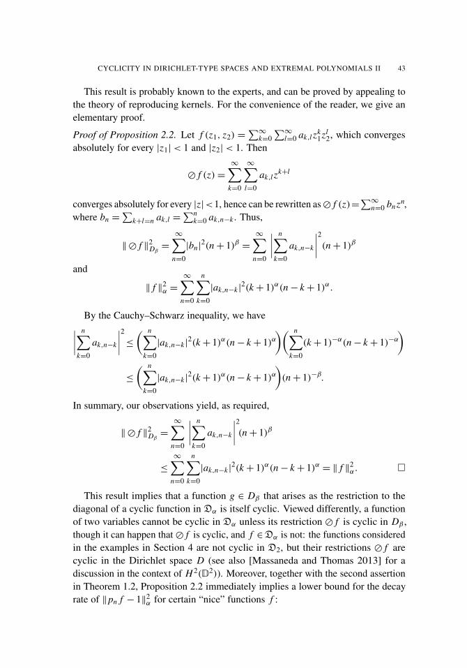
CYCLICITY IN DIRICHLET-TYPE SPACES AND EXTREMAL POLYNOMIALS II 43
This result is probably known to the experts, and can be proved by appealing tothe theory of reproducing kernels. For the convenience of the reader, we give anelementary proof.
Proof of Proposition 2.2. Let f (z1, z2) =∑∞
k=0∑∞
l=0 ak,l zk1zl
2, which convergesabsolutely for every |z1|< 1 and |z2|< 1. Then
� f (z)=∞∑
k=0
∞∑l=0
ak,l zk+l
converges absolutely for every |z|<1, hence can be rewritten as� f (z)=∑∞
n=0 bnzn,where bn =
∑k+l=n ak,l =
∑nk=0 ak,n−k . Thus,
‖� f ‖2Dβ=
∞∑n=0
|bn|2(n+ 1)β =
∞∑n=0
∣∣∣∣ n∑k=0
ak,n−k
∣∣∣∣2(n+ 1)β
and
‖ f ‖2α =∞∑
n=0
n∑k=0
|ak,n−k |2(k+ 1)α(n− k+ 1)α.
By the Cauchy–Schwarz inequality, we have∣∣∣∣ n∑k=0
ak,n−k
∣∣∣∣2≤ ( n∑k=0
|ak,n−k |2(k+ 1)α(n− k+ 1)α
)( n∑k=0
(k+ 1)−α(n− k+ 1)−α)
≤
( n∑k=0
|ak,n−k |2(k+ 1)α(n− k+ 1)α
)(n+ 1)−β.
In summary, our observations yield, as required,
‖� f ‖2Dβ=
∞∑n=0
∣∣∣∣ n∑k=0
ak,n−k
∣∣∣∣2(n+ 1)β
≤
∞∑n=0
n∑k=0
|ak,n−k |2(k+ 1)α(n− k+ 1)α = ‖ f ‖2α. �
This result implies that a function g ∈ Dβ that arises as the restriction to thediagonal of a cyclic function in Dα is itself cyclic. Viewed differently, a functionof two variables cannot be cyclic in Dα unless its restriction � f is cyclic in Dβ ,though it can happen that � f is cyclic, and f ∈Dα is not: the functions consideredin the examples in Section 4 are not cyclic in D2, but their restrictions � f arecyclic in the Dirichlet space D (see also [Massaneda and Thomas 2013] for adiscussion in the context of H 2(D2)). Moreover, together with the second assertionin Theorem 1.2, Proposition 2.2 immediately implies a lower bound for the decayrate of ‖pn f − 1‖2α for certain “nice” functions f :

44 C. BÉNÉTEAU, A. CONDORI, C. LIAW, D. SECO AND A. SOLA
Corollary 2.3. Let α≤ 2. Suppose f ∈Dα is such that the diagonal restriction� fsatisfies the hypotheses of Theorem 1.2. Then,
‖pn f − 1‖2α ≥ Cϕ−1β (n+ 1), for all pn ∈Pn.
Here, we have used that ϕ−1β (2n+ 1) is comparable to ϕ−1
β (n+ 1). We will seelater (see Proposition 2.4 and Theorem 3.1) that this decay rate is not optimal ingeneral. Note that the diagonal restrictions of the functions f (z1, z2)= 1− z1z2,f (z1, z2)= (1− z1)(1− z2), and f (z1, z2)= 1− z1 all satisfy the hypotheses.
The above remarks show how, given a cyclic function of two variables, one caneasily obtain examples of cyclic functions of one variable (although we might needto change the index α of the space in which cyclicity is being considered!) In thenext two subsections we examine how to obtain some classes of cyclic functions oftwo variables from cyclic functions of one variable, and we obtain sharp rates ofdecay in some cases.
Separable functions. Let us now consider functions of two variables that can bewritten as products of two functions of one variable:
f (z1, z2)= g(z1)h(z2).(2-1)
We shall refer to such functions as separable. Note that for such products, it followsfrom (1-1) that ‖ f ‖α = ‖g‖Dα
‖h‖Dα.
Proposition 2.4. Let α ∈ R and f be defined as in (2-1), where g, h ∈ Dα. Then,f is cyclic in Dα if and only if g and h are cyclic in Dα.
Proof. First notice that by Proposition 2.1, if f is cyclic in Dα, then g and h areconstant multiples (with respect to the fixed variable) of the slices of f , and thusare cyclic in Dα.
For the converse, suppose both g and h are cyclic in Dα. Let (pn) and (qn)
be sequences of polynomials such that ‖png− 1‖Dα→ 0 and ‖qnh− 1‖Dα
→ 0,respectively. Since the expression pngh− h = (pn(z1)g(z1)− 1)h(z2) is separable,we obtain
‖pn f − h‖α = ‖png− 1‖Dα‖h‖Dα
.
Hence, we get that h ∈ [ f ], where [ · ] denotes the cyclicity class in Dα, and so[h] ⊂ [ f ]. Since ‖qnh−1‖α = ‖qnh−1‖Dα
, the function h is cyclic in Dα and Dα
simultaneously, and the assertion follows. �
It seems natural to ask whether the growth of the extremal polynomials forseparable functions is the same as for functions in the unit disk. As we will see inTheorem 2.6, this is indeed the case. Let us first prove a lemma that will help toestablish the sharp growth restrictions.
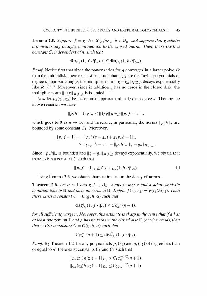
CYCLICITY IN DIRICHLET-TYPE SPACES AND EXTREMAL POLYNOMIALS II 45
Lemma 2.5. Suppose f = g · h ∈ Dα for g, h ∈ Dα, and suppose that g admitsa nonvanishing analytic continuation to the closed bidisk. Then, there exists aconstant C , independent of n, such that
distDα(1, f ·Pn)≥ C distDα
(1, h ·P2n).
Proof. Notice first that since the power series for g converges in a larger polydiskthan the unit bidisk, there exists R > 1 such that if gn are the Taylor polynomials ofdegree n approximating g, the multiplier norm ‖g−gn‖M(Dα) decays exponentiallylike R−(n+1). Moreover, since in addition g has no zeros in the closed disk, themultiplier norm ‖1/g‖M(Dα) is bounded.
Now let pn(z1, z2) be the optimal approximant to 1/ f of degree n. Then by theabove remarks, we have
‖pnh− 1/g‖α ≤ ‖1/g‖M(Dα)‖pn f − 1‖α,
which goes to 0 as n →∞, and therefore, in particular, the norms ‖pnh‖α arebounded by some constant C1. Moreover,
‖pn f − 1‖α = ‖pnh(g− gn)+ gn pnh− 1‖α≥ ‖gn pnh− 1‖α −‖pnh‖α ‖g− gn‖M(Dα).
Since ‖pnh‖α is bounded and ‖g− gn‖M(Dα) decays exponentially, we obtain thatthere exists a constant C such that
‖pn f − 1‖α ≥ C distDα(1, h ·P2n). �
Using Lemma 2.5, we obtain sharp estimates on the decay of norms.
Theorem 2.6. Let α ≤ 1 and g, h ∈ Dα. Suppose that g and h admit analyticcontinuations to D and have no zeros in D. Define f (z1, z2) = g(z1)h(z2). Thenthere exists a constant C = C(g, h, α) such that
dist2Dα(1, f ·Pn)≤ Cϕ−1
α (n+ 1),
for all sufficiently large n. Moreover, this estimate is sharp in the sense that if h hasat least one zero on T and g has no zeros in the closed disk D (or vice versa), thenthere exists a constant C = C(g, h, α) such that
Cϕ−1α (n+ 1)≤ dist2
Dα(1, f ·Pn).
Proof. By Theorem 1.2, for any polynomials pn(z1) and qn(z2) of degree less thanor equal to n, there exist constants C1 and C2 such that
‖pn(z1)g(z1)− 1‖Dα≤ C1ϕ
−1/2α (n+ 1),
‖qn(z2)h(z2)− 1‖Dα≤ C2ϕ
−1/2α (n+ 1).

46 C. BÉNÉTEAU, A. CONDORI, C. LIAW, D. SECO AND A. SOLA
Therefore,
‖pn(z1)qn(z2)g(z1)h(z2)− 1‖α≤ ‖qn(z2)h(z2)(pn(z1)g(z1)− 1)‖α +‖qn(z2)h(z2)− 1‖α
≤ ‖qnh‖α ‖png− 1‖α +‖qnh− 1‖α
= ‖qnh‖Dα‖png− 1‖Dα
+‖qnh− 1‖Dα
≤ (‖qnh− 1‖Dα+ 1)‖png− 1‖Dα
+‖qnh− 1‖Dα
≤ C2C1ϕ−1α (n+ 1)+ (C1+C2)ϕ
−1/2α (n+ 1)
≤ Cϕ−1/2α (n+ 1)
for some constant C. Therefore,
dist2Dα(1, f ·Pn)≤ Cϕ−1
α (n+ 1),
for all sufficiently large n, as desired.Moreover, the inequality is sharp. To see this, suppose h has at least one zero
on T and g has no zeros in the closed unit disk. Then, by Lemma 2.5, there exists aconstant C1 such that
(2-2) distDα(1, f ·Pn)≥ C1 distDα
(1, h ·P2n).
Note that h = h(z2), and so, by orthogonality of monomials in Dα, the quantitydistDα
(1, h ·P2n) is bounded from below by distDα(1, h ·P2n)= distDα
(1, h ·P2n).Now, by Theorem 1.2 applied to h, and again since ϕα(2n+ 1) is comparable toϕα(n+ 1), there exists a constant C2 such that
(2-3) dist2Dα(1, h ·Pn)≥ C2ϕ
−1α (n+ 1).
Thus, the inequalities in (2-2) and (2-3) imply the desired result. �
3. Norm comparisons and sharp decay of norms for the subspaces Jα,M,N
Let us now consider a third way of relating two variable cyclic functions to onevariable cyclic functions. In particular, we shall show that the polynomials in (1-2)furnish optimal approximants for a certain subclass of functions.
The subspaces Jα,M,N . In order to formulate our results, we need some notation.For −∞< α <∞ and integers M, N ≥ 1, we consider the closed subspaces
Jα,M,N ={
f ∈Dα : f =∞∑
k=0
akzMk1 zNk
2
}.
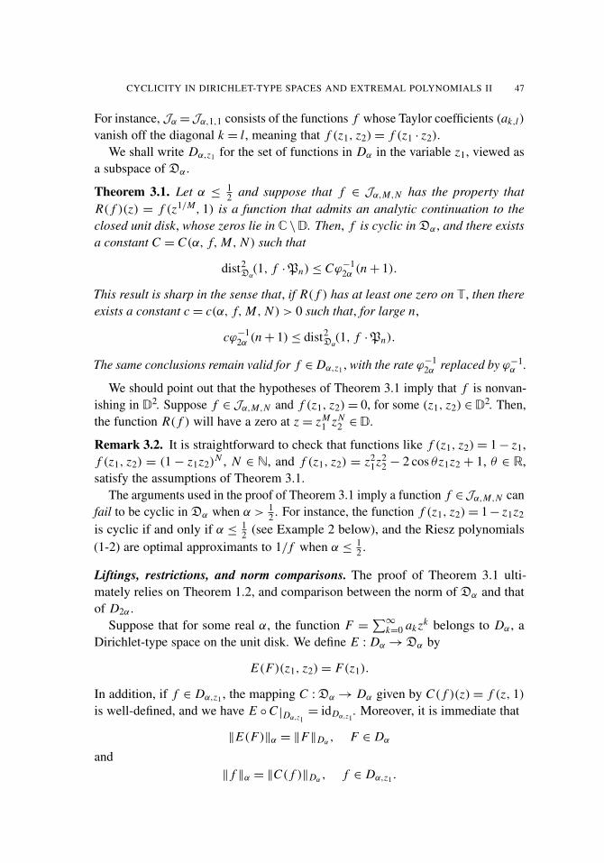
CYCLICITY IN DIRICHLET-TYPE SPACES AND EXTREMAL POLYNOMIALS II 47
For instance, Jα=Jα,1,1 consists of the functions f whose Taylor coefficients (ak,l)
vanish off the diagonal k = l, meaning that f (z1, z2)= f (z1 · z2).We shall write Dα,z1 for the set of functions in Dα in the variable z1, viewed as
a subspace of Dα.
Theorem 3.1. Let α ≤ 12 and suppose that f ∈ Jα,M,N has the property that
R( f )(z) = f (z1/M, 1) is a function that admits an analytic continuation to theclosed unit disk, whose zeros lie in C \D. Then, f is cyclic in Dα, and there existsa constant C = C(α, f,M, N ) such that
dist2Dα(1, f ·Pn)≤ Cϕ−1
2α (n+ 1).
This result is sharp in the sense that, if R( f ) has at least one zero on T, then thereexists a constant c = c(α, f,M, N ) > 0 such that, for large n,
cϕ−12α (n+ 1)≤ dist2
Dα(1, f ·Pn).
The same conclusions remain valid for f ∈ Dα,z1 , with the rate ϕ−12α replaced by ϕ−1
α .
We should point out that the hypotheses of Theorem 3.1 imply that f is nonvan-ishing in D2. Suppose f ∈ Jα,M,N and f (z1, z2)= 0, for some (z1, z2) ∈D2. Then,the function R( f ) will have a zero at z = zM
1 zN2 ∈ D.
Remark 3.2. It is straightforward to check that functions like f (z1, z2)= 1− z1,f (z1, z2) = (1− z1z2)
N , N ∈ N, and f (z1, z2) = z21z2
2 − 2 cos θ z1z2 + 1, θ ∈ R,satisfy the assumptions of Theorem 3.1.
The arguments used in the proof of Theorem 3.1 imply a function f ∈Jα,M,N canfail to be cyclic in Dα when α > 1
2 . For instance, the function f (z1, z2)= 1− z1z2
is cyclic if and only if α ≤ 12 (see Example 2 below), and the Riesz polynomials
(1-2) are optimal approximants to 1/ f when α ≤ 12 .
Liftings, restrictions, and norm comparisons. The proof of Theorem 3.1 ulti-mately relies on Theorem 1.2, and comparison between the norm of Dα and thatof D2α.
Suppose that for some real α, the function F =∑∞
k=0 akzk belongs to Dα, aDirichlet-type space on the unit disk. We define E : Dα→Dα by
E(F)(z1, z2)= F(z1).
In addition, if f ∈ Dα,z1 , the mapping C :Dα→ Dα given by C( f )(z)= f (z, 1)is well-defined, and we have E ◦C |Dα,z1
= idDα,z1. Moreover, it is immediate that
‖E(F)‖α = ‖F‖Dα, F ∈ Dα
and‖ f ‖α = ‖C( f )‖Dα
, f ∈ Dα,z1 .

48 C. BÉNÉTEAU, A. CONDORI, C. LIAW, D. SECO AND A. SOLA
Another embedding is the following one. For α ∈ R fixed, define the mappings
L M,N : D2α→Dα via L M,N (F)(z1, z2)= F(zM1 · z
N2 ),
andRM,N : Jα,M,N → D2α via RM,N ( f )(z)= f (z1/M, 1).
We initially view f (z1/M, 1) as a formal expression, but the assumption that∑k
(k+ 1)2α|ak |2 <∞
implies that f (z1/M1 , 1) is actually a well-defined holomorphic function on D; this
will become apparent below. By definition, we again have L ◦ R|Jα,M,N = idJα,M,N .
Lemma 3.3. For F ∈ D2α and f ∈ Jα,M,N , there are constants c1 = c1(α,M, N )and c2 = c2(α,M, N ) such that
‖L M,N (F)‖α ≤ c1‖F‖D2α and c2‖R( f )‖D2α ≤ ‖ f ‖α.
In particular, if f ∈ Jα,M,N , then
(3-1) c2‖R( f )‖D2α ≤ ‖ f ‖α ≤ c1‖R( f )‖D2α .
Proof. We provide the proof of the second inequality; the proof of the first isanalogous.
We first observe that for any α ∈ R and M ≥ 1, there exist constants c1(α,M)and c2(α,M) such that
c1(α,M)(k+ 1)α ≤ (Mk+ 1)α ≤ c2(α,M)(k+ 1)α,
for any k ∈ N. Thus, writing R( f )(z)=∑∞
k=0 akzk, we have
‖R( f )‖2D2α=
∞∑k=0
(k+ 1)2α|ak |2=
∞∑k=0
(k+ 1)α(k+ 1)α|ak |2
≤ [c1(α,M)c1(α, N )]−1∞∑
k=0
(Mk+ 1)α(Nk+ 1)α|ak |2
= [c1(α,M)c1(α, N )]−1‖ f ‖2α,
which proves the assertion. The two-sided bound (3-1) follows from the one-sidedbounds and the fact that f = L(R( f )). �
In particular, we see from the proof of Lemma 3.3 that in the case M = N = 1,the equalities
‖L(F)‖α = ‖F‖D2α and ‖R( f )‖D2α = ‖ f ‖α
hold; hence, R is an isometric isomorphism between Jα and D2α.
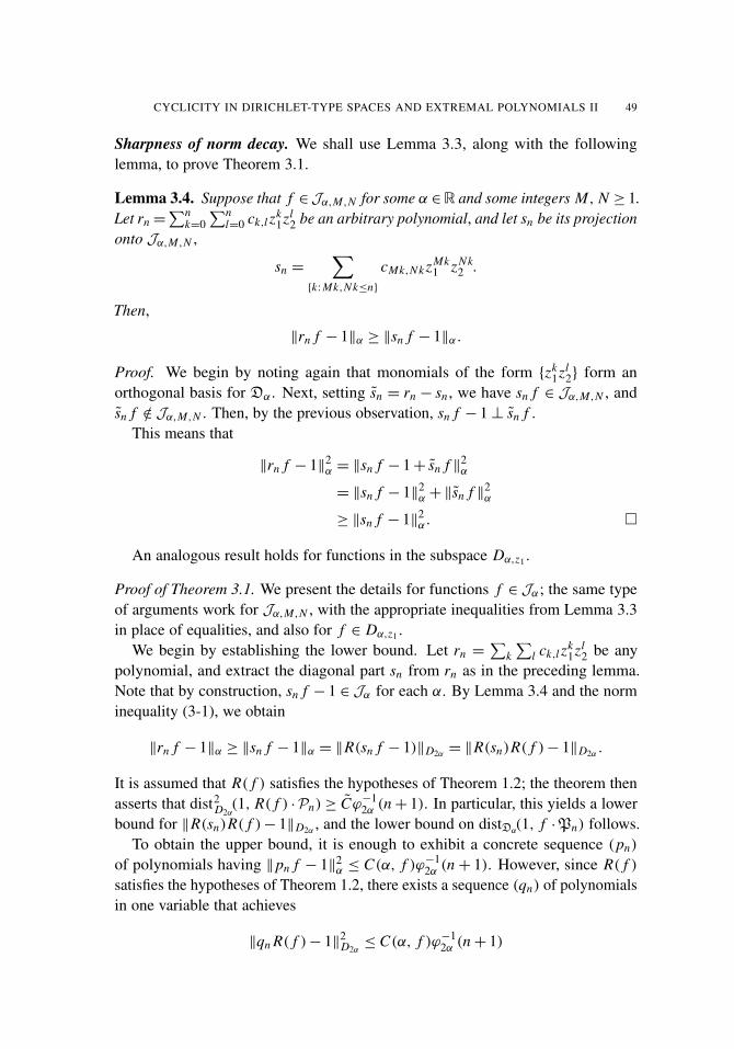
CYCLICITY IN DIRICHLET-TYPE SPACES AND EXTREMAL POLYNOMIALS II 49
Sharpness of norm decay. We shall use Lemma 3.3, along with the followinglemma, to prove Theorem 3.1.
Lemma 3.4. Suppose that f ∈Jα,M,N for some α ∈R and some integers M, N ≥ 1.Let rn =
∑nk=0
∑nl=0 ck,l zk
1zl2 be an arbitrary polynomial, and let sn be its projection
onto Jα,M,N ,
sn =∑
{k:Mk,Nk≤n}
cMk,NkzMk1 zNk
2 .
Then,
‖rn f − 1‖α ≥ ‖sn f − 1‖α.
Proof. We begin by noting again that monomials of the form {zk1zl
2} form anorthogonal basis for Dα. Next, setting sn = rn − sn , we have sn f ∈ Jα,M,N , andsn f /∈ Jα,M,N . Then, by the previous observation, sn f − 1⊥ sn f .
This means that
‖rn f − 1‖2α = ‖sn f − 1+ sn f ‖2α= ‖sn f − 1‖2α +‖sn f ‖2α≥ ‖sn f − 1‖2α. �
An analogous result holds for functions in the subspace Dα,z1 .
Proof of Theorem 3.1. We present the details for functions f ∈ Jα; the same typeof arguments work for Jα,M,N , with the appropriate inequalities from Lemma 3.3in place of equalities, and also for f ∈ Dα,z1 .
We begin by establishing the lower bound. Let rn =∑
k∑
l ck,l zk1zl
2 be anypolynomial, and extract the diagonal part sn from rn as in the preceding lemma.Note that by construction, sn f − 1 ∈ Jα for each α. By Lemma 3.4 and the norminequality (3-1), we obtain
‖rn f − 1‖α ≥ ‖sn f − 1‖α = ‖R(sn f − 1)‖D2α = ‖R(sn)R( f )− 1‖D2α .
It is assumed that R( f ) satisfies the hypotheses of Theorem 1.2; the theorem thenasserts that dist2
D2α(1, R( f ) ·Pn)≥ Cϕ−1
2α (n+ 1). In particular, this yields a lowerbound for ‖R(sn)R( f )− 1‖D2α , and the lower bound on distDα
(1, f ·Pn) follows.To obtain the upper bound, it is enough to exhibit a concrete sequence (pn)
of polynomials having ‖pn f − 1‖2α ≤ C(α, f )ϕ−12α (n+ 1). However, since R( f )
satisfies the hypotheses of Theorem 1.2, there exists a sequence (qn) of polynomialsin one variable that achieves
‖qn R( f )− 1‖2D2α≤ C(α, f )ϕ−1
2α (n+ 1)
50 C. BÉNÉTEAU, A. CONDORI, C. LIAW, D. SECO AND A. SOLA
for large enough n. But then we can define pn = L(qn) ∈ Jα, and the desiredestimate follows since
‖L(qn) f − 1‖2α = ‖R(L(qn))R( f )− 1‖2D2α= ‖qn R( f )− 1‖2D2α
by Lemma 3.3. �
Note that if R( f ) is a polynomial with only simple zeros on the unit circle T,then it is shown in [Bénéteau et al. 2015, Section 3] that the one-variable Rieszpolynomials achieve the norm decay obtained above. In the situation M = N = 1then, we have L(qn)(z1, z2)= pn(z1, z2), where pn are the Riesz-type polynomialsdefined in (1-2).
4. Polynomials with zeros on ∂D2 and measures of finite energy
Let us now examine the relationship between cyclicity and boundary zero sets offunctions in Dα. Surprisingly, some functions with large zero sets in some senseare cyclic while others with smaller zero sets are not.
Examples. Let us examine a few simple examples.
Example 1. Set f (z1, z2)= 1− z1. Then f has zero set
Z( f )= {1}×D,
a (real) 2-dimensional subset of the topological boundary of D2 which meets thedistinguished boundary along the 1-dimensional curve {1} × T. Note that f isan example of a function of the product type g(z1)h(z2) with g(z1)= 1− z1 andh(z2)= 1, and therefore by Proposition 2.4, f is cyclic in Dα if and only if α ≤ 1.
Example 2. Consider the function f (z1, z2)= 1− z1z2. The part of the zero setof f that lies on the boundary of the bidisk,
Z( f )= {(eiθ , e−iθ ) : θ ∈ [0, 2π)},
can be seen as a 1-dimensional real curve contained in the distinguished boundary T2.One verifies that all the points in Z( f ) are simple zeros. Since
1f (z1, z2)
=
∞∑k=0
∞∑l=0
δk,l zk1zl
2 =
∞∑k=0
zk1zk
2,
we have ‖1/ f ‖2−1 =
∑∞
k=0(1+ k)−2 <∞ but ‖1/ f ‖20 =∑∞
k=0 1 = +∞, so f isinvertible in the Bergman space, and indeed in Dα whenever α <−1
2 , but not inthe Hardy space of the bidisk.
Nevertheless, by Theorem 3.1, f is cyclic in Dα if and only if α ≤ 12 . Note
in particular that this function is not cyclic in the classical Dirichlet space of thebidisk!
CYCLICITY IN DIRICHLET-TYPE SPACES AND EXTREMAL POLYNOMIALS II 51
Explicit computations with the Riesz polynomials in (1-2) recover the upperbound in Theorem 3.1. Namely, we have
pn(z1, z2) f (z1, z2)− 1=−1
ϕα(n+ 1)
n+1∑k=1
[ϕα(k)−ϕα(k− 1)](z1z2)k,
and then, since |ϕα(k)−ϕα(k− 1)|2 ≤ C(α)(k− 1)−2α, we obtain
‖pn f − 1‖2α ≤C1(α)
(n+ 1)1−2α .
Thus ‖pn f − 1‖2α→ 0 as n→∞ and f is cyclic, provided that α ≤ 12 .
In fact, considering functions of the form f = 1− zM1 zN
2 for integer M, N ≥ 1instead, and performing the analogous computations, we obtain
‖pn f − 1‖2α ≤C1(α,M, N )(n+ 1)1−2α(4-1)
with a constant C1(α,M, N ) which does not depend on n.
Example 3. We examine f (z1, z2) = 1− z1− z2+ z1z2 = (1− z1)(1− z2). Thezero set of f is
Z( f )= ({1}×D)∪ (D×{1}),
a 2-dimensional set that extends into the topological boundary of the bidisk. Itsintersection with T2 consists of the curves
Z( f )= ({1}×T)∪ (T×{1}).
All zeros of f are simple, except the point (1, 1), which has order 2. Since
1f (z1, z2)
=
∞∑k=0
∞∑l=0
zk1zl
2,
it follows that 1/ f /∈ A2(D2). Note that again, f is separable with g(z1)= 1− z1
and h(z2)= 1− z2, and therefore f is cyclic in Dα if and only if α ≤ 1.In this case, computing with the Riesz polynomials leads to misleading estimates.
Defining polynomials pn , as before, via (1-2), we compute
pn f =−1
(n+ 1)1−α
n+1∑k=1
[k1−α− (k− 1)1−α](zk
1+ zk2)
+1
(n+ 1)1−α
n+1∑k=1
[k1−α− (k− 1)1−α]zk
1zk2.

52 C. BÉNÉTEAU, A. CONDORI, C. LIAW, D. SECO AND A. SOLA
We use the estimates from the previous example, and exploit the one-variableestimates from [Bénéteau et al. 2015], to obtain
‖pn f − 1‖2Dα=
2(n+ 1)2−2α
n+1∑k=1
(k+ 1)α[k1−α− (k− 1)1−α]2
+1
(n+ 1)2−2α
n+1∑k=1
(k+ 1)2α[k1−α− (k− 1)1−α]2
≤c1(α)
(n+ 1)1−α+
c2(α)
(n+ 1)1−2α .
The first term in the right-hand side dominates when α < 0, whereas the secondis larger when α > 0. In particular, the estimate does show that f is cyclic in Dα
provided α ≤ 12 . However, as we have seen, the rate is not optimal, and f remains
cyclic when α > 12 .
Note the interesting contrast between Example 2 and Example 3: the function inExample 2 is not cyclic in the (classical) Dirichlet space of the bidisk, and yet insome sense has a much smaller zero set than the function in Example 3, which iscyclic! On the other hand, as a kind of dual phenomenon, f = 1− z1z2 exhibits afaster rate of decay of norms ‖pn f −1‖α for α < 0 than does f = (1− z1)(1− z2).
Example 4. The polynomial f (z1, z2)= 1− (z1+ z2)/2 has no zeros in D2, andvanishes at a single boundary point: Z( f )= {(1, 1)} ⊂ T2.
In [Hedenmalm 1988, Section 4], it is proved that if f ∈D2 has Z( f )= {(1, 1)},and both f ( · , 1) and f (1, · ) are outer functions, then the closure of the principalideal generated by f coincides with the closed ideal
I({(1, 1)}
)= { f ∈D2 : f (1, 1)= 0}.
(Hedenmalm’s norm is defined using the weights (1+ k2)(1+ l2) but is equivalentto the norm in D2.) Since the norm of D1 is weaker than that of D2, it follows thatsuch functions are cyclic in Dα for α≤ 1 as the D1-closure of the invariant subspaceI({(1, 1)}
)⊂D2 coincides with [ f ], and contains the cyclic function 1− z1.
In particular, the polynomial f (z1, z2)= 1− (z1+ z2)/2 is cyclic in Dα , for allα≤ 1. (An independent proof of this fact has been given by T. J. Ransford [personalcommunication, 2014].) Computing with polynomials of the form
pn(z1, z2)=
n∑k=0
(1−
ϕα(k)ϕα(n+ 1)
)(z1+ z2)
k
2k
CYCLICITY IN DIRICHLET-TYPE SPACES AND EXTREMAL POLYNOMIALS II 53
and using the fact that (z1+ z2)k1 ⊥ (z1+ z2)
k2 when k1 6= k2, one finds that
‖pn f − 1‖2α =n+1∑k=1
4−k(
k1−α− (k− 1)1−α
(n+ 1)1−α
)2 k∑j=0
(kj
)2
( j + 1)α(k− j + 1)α.
Using the bound
( j + 1)α(k− j + 1)α ≤ C(k+ 1)2α, 0≤ j ≤ k,
together with the identityk∑
j=0
(kj
)2
=
(2kk
)and standard estimates on binomial coefficients, we obtain the estimate
dist2Dα(1, (2− z1− z2) ·Pn)≤ Cϕ2α−1/2(n+ 1).
Unfortunately, we have not been able to obtain a sharp estimate, but the above boundshows that the optimal rate is different from the two rates we have seen previously.
Measures of finite energy. It would be interesting to understand the relationshipbetween cyclicity and boundary zero sets — in particular, given a function f , tofind a measure whose support lies on the zero set of the boundary values of f thatrelates to the cyclicity properties of f .
We now give a necessary condition for a function to be cyclic. This conditioninvolves the notion of capacity, and represents a straightforward generalization ofresults of Brown and Shields in the one-variable case.
Definition 4.1. Let E ⊂ T2 be a Borel set. We say that a probability measure µsupported in E has finite logarithmic energy if
I [µ] =∫
T2
∫T2
loge
|eiθ1 − eiϑ1 |log
e|eiθ2 − eiϑ2 |
dµ(θ1, θ2) dµ(ϑ1, ϑ2) <∞.
If E supports no such measure, we say that E has logarithmic capacity 0.
The integral defining the energy I [µ] can be seen as a convolution with kernel
h(s, t)= loge
|1− eis |log
e|1− ei t |
.
Replacing the logarithmic product kernel in the definitions above with
hα(s, t)=1
|1− eis |1−α
1|1− ei t |1−α
,
one obtains the notions of Riesz energy, denoted by Iα[µ], and Riesz capacity oforder 0< α < 1.

54 C. BÉNÉTEAU, A. CONDORI, C. LIAW, D. SECO AND A. SOLA
The α-energy of µ can be expressed in terms of its Fourier coefficients
µ(k, l)=∫
T2e−i(kθ1+lθ2) dµ(θ1, θ2), k, l ∈ Z.
Namely, we have (compare [El-Fallah et al. 2014, Chapter 2], for instance)
Iα[µ] =∞∑
k=−∞
∞∑l=−∞
hα(k, l)|µ(k, l)|2.
Computing the Fourier coefficients h(k, l) (see [Brown and Shields 1984, p. 294]for details), we find that
(4-2) I [µ] = 1+∞∑
k=1
|µ(k, 0)|2
k+
∞∑l=1
|µ(0, l)|2
l+
12
∑k∈Z\{0}
∞∑l=1
|µ(k, l)|2
|k|l.
Similarly, one can show (again see [El-Fallah et al. 2014, Chapter 2]) that theFourier coefficients of hα satisfy
c1(|k| + 1)−α (|l| + 1)−α ≤ |hα(k, l)| ≤ c2(|k| + 1)−α (|l| + 1)−α
for some constants 0< c1 < c2 <∞.The notion of energy now allows us to identify some noncyclic f ∈ Dα by
looking at their boundary zero sets. To make this notion precise, we note that onecan show that functions f ∈Dα have radial limits
f ∗(eiθ1, eiθ2)= limr→1−
f (reiθ1, reiθ2)
quasi-everywhere with respect to the appropriate capacity. That is, the limit existsfor all points outside a set of capacity 0, and hence it makes sense to speak of thecapacity of the set Z( f ∗). (In fact, Kaptanoglu considers more general approachregions in [Kaptanoglu 1994], but we do not need this here.)
Proposition 4.2. If f ∈D and Z( f ∗) has positive logarithmic capacity, then f isnot cyclic.
Proof. The proof is completely analogous to that of [Brown and Shields 1984,Theorem 5]; we refer the reader to the paper of Brown and Shields for details andpresent the arguments in condensed form here.
The key idea is to identify the Bergman space A2(D2) with the dual of D viathe pairing
〈 f, g〉 =∞∑
k=0
∞∑l=0
ak,lbk,l,
where f =∑k,l
ak,l zk1zl
2 ∈D and g =∑k,l
bk,l zk1zl
2 ∈ A2(D2). We then consider the

CYCLICITY IN DIRICHLET-TYPE SPACES AND EXTREMAL POLYNOMIALS II 55
Cauchy integral
C[µ] =∫
T2(1− eiθ1 z1)
−1 (1− eiθ2 z2)−1 dµ(θ1, θ2)
of µ, a measure of finite logarithmic energy with supp(µ)⊂ Z( f ∗). A comparisonwith (4-2) then reveals that
‖C[µ]‖2A2(D2)=
∞∑k=0
∞∑l=0
|µ(k, l)|2
(k+ 1)(l + 1)<∞
so that C[µ] induces a nontrivial element of D∗. On the other hand, since themeasure µ is supported on Z( f ∗) by assumption, the functional induced by C[µ]annihilates [ f ], and so f is not cyclic. �
For 0< α < 1, the same result holds once we replace logarithmic capacity withRiesz capacity and make the identification (Dα)
∗=D−α in the proof.
The argument used in the proof of Proposition 4.2 can be used to give anotherproof of the noncyclicity of the function f (z1, z2) = 1 − z1z2 in D. Namely,consider the probability measure µZ on T2 induced by the (normalized) integrationcurrent associated with the variety Z(1− z1z2) ∩ T2 (see [Lelong and Gruman1986, Chapter 2] for the relevant definitions). A quick computation reveals thatµZ(k, l) = δkl , so that C[µZ ](z1, z2) = 1/(1− z1z2), a function in the Bergmanspace of the bidisk which satisfies⟨
zk1zl
2 f,C[µZ ]⟩= 0, for all k, l ≥ 0.
In fact, Z(1− z1z2)∩T2 has positive Riesz capacity precisely when α > 12 .
5. Concluding remarks and open problems
It appears to be a difficult task to characterize the cyclic elements of Dα for α ≤ 1,and many basic questions remain. For instance, it is natural to ask whether theBrown–Shields conjecture is true for functions on the bidisk.
Problem 5.1. Is the condition that f ∈ D is outer and Z( f ∗) has logarithmiccapacity 0 sufficient for f to be cyclic?
This question remains open for the Dirichlet space of the unit disk, and is widelyconsidered to be a challenging problem. A first step towards understanding cyclicfunctions in Dα might be to solve the following natural problem.
Problem 5.2. Characterize the cyclic polynomials f ∈Dα for each α ∈ (0, 1].
An obvious necessary condition for f to be cyclic is that Z( f )∩D2=∅, and
if f is a polynomial that does not vanish in D2, then f is cyclic because both fand 1/ f extend analytically to a larger polydisk. But the problem appears to be
56 C. BÉNÉTEAU, A. CONDORI, C. LIAW, D. SECO AND A. SOLA
open for polynomials with Z( f ) ∩ ∂D26= ∅: we would at least like to identify
the polynomials whose zero sets have positive capacity. We have proved thatpolynomials that are products of polynomials in one variable are cyclic, and so thezero sets associated with such functions must all have zero capacity.
As we have seen in our examples, it can happen that a polynomial with a largerzero set, in the topological sense and in the sense of measure, is cyclic in Dα forsome α, while a polynomial with a smaller zero set is not. We have also noted thata polynomial that fails to be cyclic in Dα when α > 1
2 can be “more” cyclic in Dα ,for α < 0, than polynomials that are cyclic in all Dα . We mean this in the sense that
dist2Dα(1, (1− z1z2) ·Pn) � Cϕ−1
2α (n+ 1)
whiledist2
Dα(1, (1− z1)(1− z2) ·Pn) � Cϕ−1
α (n+ 1).
It would be interesting to develop a rigorous understanding of this phenomenon.
Acknowledgments
The authors wish to thank Thomas Ransford and Stefan Richter for interestingconversations and helpful suggestions. Thanks are due to the referee for a carefulreading of the paper.
References
[Bénéteau et al. 2015] C. Bénéteau, A. A. Condori, C. Liaw, D. Seco, and A. A. Sola, “Cyclic-ity in Dirichlet-type spaces and extremal polynomials”, J. Analyse Math. 126 (2015), 259–286.arXiv 1301.4375
[Brown and Shields 1984] L. Brown and A. L. Shields, “Cyclic vectors in the Dirichlet space”, Trans.Amer. Math. Soc. 285:1 (1984), 269–303. MR 86d:30079 Zbl 0517.30040
[Douglas and Yang 2000] R. G. Douglas and R. Yang, “Operator theory in the Hardy space overthe bidisk (I)”, Integral Equations Operator Theory 38:2 (2000), 207–221. MR 2002m:47006Zbl 0970.47016
[El-Fallah et al. 2014] O. El-Fallah, K. Kellay, J. Mashreghi, and T. Ransford, A primer on the Dirich-let space, Cambridge Tracts in Mathematics 203, Cambridge University Press, 2014. MR 3185375Zbl 1304.30002
[Gelca 1995] R. Gelca, “Rings with topologies induced by spaces of functions”, Houston J. Math.21:2 (1995), 395–405. MR 96h:46075 Zbl 0849.46036 arXiv funct-an/9604006
[Hedenmalm 1988] H. Hedenmalm, “Outer functions in function algebras on the bidisc”, Trans. Amer.Math. Soc. 306:2 (1988), 697–714. MR 90c:32007 Zbl 0655.32017
[Hörmander 1990] L. Hörmander, An introduction to complex analysis in several variables, 3rded., North-Holland Mathematical Library 7, North-Holland, Amsterdam, 1990. MR 91a:32001Zbl 0685.32001
[Horowitz and Oberlin 1975] C. Horowitz and D. M. Oberlin, “Restriction of H p functions to thediagonal of Un”, Indiana Univ. Math. J. 24:8 (1975), 767–772. MR 50 #7583 Zbl 0282.32001
CYCLICITY IN DIRICHLET-TYPE SPACES AND EXTREMAL POLYNOMIALS II 57
[Jupiter and Redett 2006] D. Jupiter and D. Redett, “Multipliers on Dirichlet type spaces”, Acta Sci.Math. (Szeged) 72:1-2 (2006), 179–203. MR 2007f:47023 Zbl 1174.46320 arXiv math/0510193
[Kaptanoglu 1994] H. T. Kaptanoglu, “Möbius-invariant Hilbert spaces in polydiscs”, Pacific J. Math.163:2 (1994), 337–360. MR 94m:46044 Zbl 0791.32015
[Lelong and Gruman 1986] P. Lelong and L. Gruman, Entire functions of several complex variables,Grundlehren der Mathematischen Wissenschaften 282, Springer, Berlin, 1986. MR 87j:32001Zbl 0583.32001
[Mandrekar 1988] V. Mandrekar, “The validity of Beurling theorems in polydiscs”, Proc. Amer. Math.Soc. 103:1 (1988), 145–148. MR 90c:32008 Zbl 0658.47033
[Massaneda and Thomas 2013] X. Massaneda and P. J. Thomas, “Non cyclic functions in the Hardyspace of the bidisc with arbitrary decrease”, preprint, 2013. arXiv 1301.2622
[Redett and Tung 2010] D. Redett and J. Tung, “Invariant subspaces in Bergman space over thebidisc”, Proc. Amer. Math. Soc. 138:7 (2010), 2425–2430. MR 2011d:47021 Zbl 1193.47013
[Richter and Sundberg 2012] S. Richter and C. Sundberg, “Cyclic vectors in the Drury–Arvesonspace”, slides, 2012, http://math.utk.edu/~richter/talk/Richter_Cyclic_Drury_Arveson2012.pdf.
[Rudin 1969] W. Rudin, Function theory in polydiscs, W. A. Benjamin, New York, 1969. MR 41#501 Zbl 0177.34101
[Stegenga 1980] D. A. Stegenga, “Multipliers of the Dirichlet space”, Illinois J. Math. 24:1 (1980),113–139. MR 81a:30027 Zbl 0432.30016
[Taylor 1966] G. D. Taylor, “Multipliers on Dα”, Trans. Amer. Math. Soc. 123 (1966), 229–240.MR 34 #6514 Zbl 0166.12003
Received October 15, 2013. Revised September 10, 2014.
CATHERINE BÉNÉTEAU
DEPARTMENT OF MATHEMATICS
UNIVERSITY OF SOUTH FLORIDA
4202 E. FOWLER AVENUE
TAMPA, FL 33620-5700UNITED STATES
ALBERTO A. CONDORI
DEPARTMENT OF MATHEMATICS
FLORIDA GULF COAST UNIVERSITY
10501 FGCU BOULEVARD SOUTH
FORT MYERS, FL 33965-6565UNITED STATES
CONSTANZE LIAW
CASPER AND DEPARTMENT OF MATHEMATICS
BAYLOR UNIVERSITY
ONE BEAR PLACE #97328WACO, TX 76798-7328UNITED STATES
58 C. BÉNÉTEAU, A. CONDORI, C. LIAW, D. SECO AND A. SOLA
DANIEL SECO
MATHEMATICS INSTITUTE
UNIVERSITY OF WARWICK
ZEEMAN BUILDING
COVENTRY
CV4 7ALUNITED KINGDOM
ALAN A. SOLA
CENTRE FOR MATHEMATICAL SCIENCES
UNIVERSITY OF CAMBRIDGE
WILBERFORCE ROAD
CAMBRIDGE
CB3 0WBUNITED KINGDOM

PACIFIC JOURNAL OF MATHEMATICSVol. 276, No. 1, 2015
dx.doi.org/10.2140/pjm.2015.276.59
COMPACTNESS RESULTS FOR SEQUENCES OFAPPROXIMATE BIHARMONIC MAPS
CHRISTINE BREINER AND TOBIAS LAMM
We will prove energy quantization for approximate (intrinsic and extrinsic)biharmonic maps into spheres where the approximate map is in L log L.Moreover, we demonstrate that if the L log L norm of the approximatemaps does not concentrate, the images of the bubbles are connected withoutnecks.
1. Introduction
Critical points to the Dirichlet energy
E.u/ WD1
2
Z�
jDuj2 dx
are called harmonic maps, and the compactness theory for such a sequence intwo dimensions is well understood. Let � � R2 be a bounded domain and N
a smooth, compact Riemannian manifold. For a sequence of harmonic mapsuk 2 W 1;2.�;N / with uniform energy bounds, Sacks and Uhlenbeck [1981]proved that a subsequence uk converges weakly to a harmonic u1 on � anduk ! u1 in C1.� n fx1; : : : ;x`g/ for some finite ` depending on the energybound. For each xi , they showed that there exist some number of “bubbles”, maps�ij W S2 ! N , that result from appropriate conformal scalings of the sequenceuk near xi . In dimension 2, E.u/ is conformally invariant and thus one can askwhether any energy is lost in the limit. Jost [1991] proved that in fact the energy isquantized; there is no unaccounted energy loss:
limk!1
E.uk/DE.u1/CXiD1
`iXjD1
E.�ij /:
Parker [1996] provided the complete description of the C 0 limit or “bubble tree”.In particular, he demonstrated that the images of the limiting map u1 and thebubbles �ij are connected without necks. Around the same time, various authors
Breiner was supported in part by NSF grant DMS-1308420 and an AMS-Simons Travel Grant.MSC2010: primary 35J60, 35J48; secondary 58E20.Keywords: harmonic maps, biharmonic maps, bubbling, energy quantization.
59

60 CHRISTINE BREINER AND TOBIAS LAMM
proved energy quantization and the no-neck property for approximate harmonicmaps [Ding and Tian 1995; Wang 1996; Qing and Tian 1997; Lin and Wang 1998;Chen and Tian 1999].
In this paper, we are interested in an analogous compactness problem for ascale-invariant energy in four dimensions. Let .M 4;g/ and .N k ; h/ be compactRiemannian manifolds without boundary, with N k isometrically embedded in someRn. Consider the energy functional
Eext.u/ WD
ZM
j�uj2 dx
for u 2W 2;2.M;N /, where � is the Laplace–Beltrami operator. Critical pointsto this functional are called extrinsic biharmonic maps, and the Euler–Lagrangeequation satisfied by such maps is of fourth order. Clearly, this functional dependsupon the immersion of N into Rn. To avoid such a dependence, one may insteadconsider critical points to the functional
Eint.u/ WD
ZM
ˇ.�u/T
ˇ2dx;
where .�u/T is the projection of �u onto TuN . Critical points to this functionalare called intrinsic biharmonic maps. The Euler–Lagrange equations satisfied byextrinsic and intrinsic biharmonic maps have been computed (see, for instance,[Wang 2004b]). We will be interested in approximate critical points.
Definition 1.1. Let u 2 W 2;2.B1;N /, where B1 � R4 and N is a C 3 closedsubmanifold of some Rn. Let f 2L log L.B1;R
n/. Then u is an f-approximatebiharmonic map if
�2u��.A.u/.Du;Du//� 2d�h�u;DP .u/iC h�.P .u//;�ui D f:
We call u an f-approximate intrinsic biharmonic map if
�2u��.A.u/.Du;Du//� 2d�h�u;DP .u/i
C h�.P .u//;�ui �P .u/.A.u/.Du;Du/DuA.u/.Du;Du//
� 2A.u/.Du;Du/A.u/.Du;DP .u//D f:
Here A is the second fundamental form of N ,! Rn and P .u/ W Rn! TuN is theorthogonal projection from Rn to the tangent space of N at u.
Recently, Hornung and Moser [2012], Laurain and Rivière [2013], and Wangand Zheng [2012] determined the energy quantization result for sequences ofintrinsic biharmonic maps, approximate intrinsic and extrinsic biharmonic maps,and approximate extrinsic biharmonic maps, respectively. (In fact, the result of
COMPACTNESS RESULTS FOR SEQUENCES OF APPROXIMATE BIHARMONIC MAPS 61
[Laurain and Rivière 2013] applies to a broader class of solutions to scaling-invariantvariational problems in dimension four.)
As a first result, we demonstrate that when the target manifold is a sphere,the energy quantization result extends to f-approximate biharmonic maps withf 2L log L. For the definition of this Banach space, see the appendix.
Theorem 1.2. Let fk 2L log L.B1;RnC1/ and uk 2W 2;2.B1;S
n/ a sequence offk-approximate biharmonic maps with
(1-1) kD2ukkL2.B1/CkDukkL4.B1/
CkfkkL log L.B1/ �ƒ<1:
If uk *u weakly in W 2;2.B1;Sn/, there exists fx1; : : : ;x`g�B1 such that uk!u
in W2;2
loc .B1 n fx1; : : : ;x`g;Sn/.
Moreover, for each 1 � i � ` there exists an `i 2 N and nontrivial, smoothbiharmonic maps !ij 2 C1.R4;Sn/ with finite energy (1� j � `i) such that
limk!1
ZBri
.xi /
jD2uk j2D
ZBri
.xi /
jD2uj2C
`iXjD1
ZR4
jD2!ij j2;
limk!1
ZBri
.xi /
jDuk j4D
ZBri
.xi /
jDuj4C
`iXjD1
ZR4
jD!ij j4:
Here ri D12
min1�j�`;j¤ifjxi �xj j; dist.xi ; @B1/g.
As a second result, we demonstrate the no-neck property for approximate bihar-monic maps with the approximating functions L log L norm not concentrating.
Theorem 1.3. Let fk 2L log L such that the L log L norm does not concentrate.For uk a sequence of fk-approximate biharmonic maps satisfying (1-1), the imagesof u and the maps !ij described above are connected in Sn without necks.
In particular, if fk 2�.L/, an Orlicz space such that limt!1 �.t/=.t log t/D1,the theorem holds. For a definition of an Orlicz space, see the appendix.
Remark 1.4. The theorems also hold for uk a sequence of fk-approximate intrin-sic biharmonic maps. We will prove the theorems in detail for fk-approximatebiharmonic maps, and point out the necessary changes one must make to prove theintrinsic case.
We consider biharmonic maps into spheres because the symmetry of the targetprovides structure for the equation that can be exploited to prove higher regularity.For an f-approximate biharmonic map into Sn, the structural equations takes theform (see [Wang 2004a])
(1-2) d�.D�u^u��u^Du/D f ^u;

62 CHRISTINE BREINER AND TOBIAS LAMM
and, for an f-approximate intrinsic biharmonic u,
(1-3) d�.D�u^u��u^DuC 2jDuj2Du^u/D f ^u:
The structure of the equation for harmonic maps from a compact Riemann surfaceinto Sn was determined independently by Chen [1989] and Shatah [1988]. Theydemonstrated that u satisfies the conservation law
d�.Du^u/D 0:
Hélein [1990] used the structure of this equation and Wente’s inequality [1969] todetermine that any weakly harmonic u 2W 1;2 was in fact C1.
Li and Zhu [2011] used this additional structure to determine energy quantizationfor approximate harmonic maps. In their setting, the equation takes the formd�.Du^u/D � ^u for � 2L log L. Our proof of energy quantization is similarin spirit to their work and to the recent small-energy compactness result of Sharpand Topping [2013]. Of critical importance are the energy estimates we prove inSection 2. The first estimates, from Proposition 2.1, are used in two ways. First, theLp estimates of (2-2), (2-3) provide sufficient control to determine a small-energycompactness result away from the bubbles. Second, we use the Lorentz space dualityto prove energy quantization and thus require uniform bounds on the appropriateLorentz energies as in (2-1). In Section 3 we prove the energy quantization result.We point out that since the oscillation bound contains an energy term of the formkD�ukkL4=3 , we must also prove this energy is quantized. This point justifies thenecessity of the estimate (2-4). We prove the energy quantization result, under thepresumption of the occurrence of one bubble, in Proposition 3.4.
We next use this stronger energy quantization result for maps into spheres toprove a no-neck property. Zhu [2012] showed the no-neck property for approximateharmonic maps with � in a space essentially between Lp with p > 1 and L log L.For w a cutoff function of the approximate harmonic map u, Zhu considered aHodge decomposition of the 1-form ˇ WDDw^u. (This is actually a matrix of 1-forms, but we gloss over that point for now.) He bounded kˇkL2;1 by bounding eachcomponent of the decomposition, and used this to bound kDwkL2;1 by kDukL2
plus a norm of the torsion term, � . Using "-compactness and a simple dualityargument, he showed the oscillation of u is controlled by kDwkL2;1 , which in turnimplies the desired result.
Like Zhu, we prove the no-neck property by demonstrating that the oscillationof an f-approximate biharmonic map is controlled by norms that tend to zero inthe neck region. Using a duality argument, we first determine that the oscillationof u on an annular region is bounded by quantized energy terms plus a thirdderivative of a cutoff function w. Our main work is in determining an appropriateestimate for kD�wkL4=3;1 . We determine this bound by considering the 1-form

COMPACTNESS RESULTS FOR SEQUENCES OF APPROXIMATE BIHARMONIC MAPS 63
ˇ D D�w ^ u��w ^Du, and we bound D�w by bounding ˇ via its Hodgedecomposition. In particular, we take advantage of the divergence structure of theequation for biharmonic maps into spheres to show that ˇ not only has good L4=3
estimates but in fact has good estimates in L4=3;1. This second estimate allowsus to prove the necessary oscillation lemma. The proof of the oscillation lemmaconstitutes the work of Section 4. Coupling the oscillation lemma with energyquantization, we prove Theorem 1.3 in Section 5.
Finally, the arguments we use require a familiarity with Lorentz spaces andthe appropriate embedding theorems relevant in dimension four. In the appendix,we describe the various Banach spaces and collect the necessary embeddingsand estimates.
Many steps of the proof require the use of cutoff functions, so we set:
Definition 1.5. Let �2C10.B2/with ��1 in B1. For all r>0 set �r .x/D�.x=r/.
Note added in proof: As we finalized the paper, we noticed a somewhat relatedpreprint [Liu and Yin 2013], in which the authors claim that the no-neck propertyholds for sequences of biharmonic maps into general targets. Their methods arequite different from ours and we believe our results are of independent interest.
2. Energy estimates
To establish strong convergence away from points of energy concentration, we firstprove the necessary energy estimates. The small-energy compactness result relieson the fact that in both (2-2) and (2-3) there is an extra power of the energy on theright-hand side of the inequality. Thus, small energy implies that kDukkL4 andkD2ukkL2 must converge to zero on small balls. Measure-theoretic arguments inthe next section will then imply strong convergence for these norms to some Du
and D2u respectively.
Proposition 2.1. Let u 2 W 2;2.B2;Sn/ be an f-approximate (intrinsic) bihar-
monic map, where f 2L log L.B2;RnC1/. Then there exists C > 0 such that
(2-1) kD3ukL4=3;1.B1/CkD2ukL2;1.B1/
CkDukL4;1.B1/
� C.kD2uk2L2.B2/
CkDuk2L2.B2/
CkDukL2.B2/
Ckf kL log L.B2/
/:
Moreover, there exists Q" > 0 such that, if
kD2ukL2.B2/CkDukL4.B2/
< Q";
then, for every 0< r < 12
,
kD2uk2L2.Br /
� C r2kD2uk2
L2.B2/
CC.kD2uk4L2.B2/
CkDuk4L4.B2/
Ckf k2L1.B2/
kf kL log L.B2/
/;
(2-2)

64 CHRISTINE BREINER AND TOBIAS LAMM
kDuk4L4.Br /
� C r4kDuk4
L2.B2/
CC.kD2uk8L2.B2/
CkDuk8L4.B2/
Ckf k3L1.B2/
kf kL log L.B2/
/;
(2-3)
kD�uk4=3
L4=3.Br /� C r4=3
kD2uk4=3
L2.B2/
CC.kD2uk8=3
L2.B2/CkDuk
8=3
L4.B2/Ckf k
1=3
L1.B2/kf k
L log L.B2//:
(2-4)
Remark 2.2. In point of fact, we do not need the full strength of (2-4) in application.We use instead the estimate
kD�uk4=3
L4=3.Br /�C.kD2uk
4=3
L2.B8r /CkDuk
4=3
L4.B8r /Ckf k
1=3
L1.B8r /kf k
L log L.B8r //;
which can be immediately proven via the method outlined below.
Proof. First, find v 2W1;2
0.B
2; so.nC 1//\W 2;2.B
2; so.nC 1// such that
�v D�u^u:
Thus, for each i; j 2 f1; : : : ; nC 1g, �vij D uj�ui � ui�uj . It follows from(1-2) that
�2v D�.�u^u/D 2d�.�u^Du/Cf ^u:
Next we let � 2W2;2
0.B
2; so.nC 1/˝�1R4/ be the solution of
�2� D d�.2�u^Du/:
Here so.nC 1/˝�1R4 denotes the space of 1-forms tensored with .nC1/�.nC1/-antisymmetric matrices. Using Calderón–Zygmund theory coupled with interpola-tion, and using the estimates from Section A.2, we determine that
(2-5) kD3�kL4=3;1.B2/CkD2�kL2;1.B2/
CkD�kL4;1.B2/
� c.kD2uk2L2.B2/
CkDuk2L2.B2/
/:
Moreover, letting 2W2;2
0.B2; so.nC 1// be the solution of
�2 D f ^u;
we conclude that
(2-6) kD kL4;1.B2/CkD2 kL2;1.B2/
CkD3 kL4=3;1.B2/� ckf kL log L.B2/:
Defining
B WD v�� �

COMPACTNESS RESULTS FOR SEQUENCES OF APPROXIMATE BIHARMONIC MAPS 65
and using the above equation for v, we conclude that each Bij is a biharmonicfunction on B2. Now every biharmonic function satisfies the mean value property
B.x/D c1 �
ZBr .x/
B.y/ dy � c2 �
ZB2r .x/
B.y/ dy;
for every B2r .x/� B2 (see, e.g., [Huilgol 1971]). Hence we estimate
kD2BkL2;1.B3=2/CkD3BkL4=3;1.B3=2/
� ckDBkL2.B2/
� c.kDvkL2.B2/Ckf kL log L.B2/CkD
2uk2L2.B2/
CkDuk2L2.B2/
/:
Since v D 0 on @B2, we can use the divergence theorem and Cauchy–Schwarz toshow that Z
B2
jDvijj2D�
ZB2
vij�vijD�
ZB2
Dvij� .Du^u/ij
�1
2
ZB2
jDvijj2CC
ZB2
jDuj2:
Thus,
kD2BkL2;1.B3=2/CkD3BkL4=3;1.B3=2/
� c.kDukL2.B2/
Ckf kL log L.B2/
CkD2uk2L2.B2/
CkDuk2L2.B2/
/:
Now we observe that, since �v D�u^u,
�uD .�u^u/:uCh�u;uiuD�v:u� jDuj2u;
where here �:u represents matrix multiplication. Therefore,
�2uD�.�v:u� jDuj2u/D d�.D�v:uC�v:Du�D.jDuj2u//:
To get the second- and third-derivative estimates in (2-1), we first observe that
kD2vkL2;1.B3=2/CkD3vkL4=3;1.B3=2/
� c.kDukL2.B2/
Ckf kL log L.B2/
CkD2uk2L2.B2/
CkDuk2L2.B2/
/:
Using the previous estimates and Section A.2, we observe that the 1-form in theparentheses is in L4=3;1. Lemma A.3 in [Lamm and Rivière 2008] implies that
kD2ukL2;1.B1/CkD3ukL4=3;1.B1/
� c.kD3vkL4=3;1.B3=2/
CkD2vk2L2.B2/
CkD2uk2L2.B2/
CkDuk2L2.B2/
/
� c.kDukL2.B2/
Ckf kL log L.B2/
CkD2uk2L2.B2/
CkDuk2L2.B2/
/:

66 CHRISTINE BREINER AND TOBIAS LAMM
Finally, Sobolev embedding for Lorentz spaces implies that
kDukL4;1.B1/� c.kD2ukL2;1.B2/
CkDukL2;1.B2//
� c.kD2ukL2;1.B2/CkDukL2.B2/
/:
Combining this with the previous estimates finishes the proof of (2-1).To prove the small-energy estimates, we observe that u satisfies (see, for instance,
[Lamm and Rivière 2008, Equations 1.4 and 1.14])
(2-7) �2uD�.V �Du/C d�.wDu/CW �DuCf;
where V ij D uiDuj �uj Dui , wij D�d�.V ij /� 2jDuj2ıij , and
W ijD�D.d�.V ij //C 2.�uiDuj
��uj Dui/:
Let Mm denote the space of m � m matrices and Mm ˝ �kR4 the space of
k-forms tensored with m �m matrices. Then V 2 W 1;2.B2;MnC1 ˝�1R4/,
w 2L2.B2;MnC1/, and W 2W �1;2.B2, MnC1˝�1R4/.
Without loss of generality we extend f by zero outside of B2. The small-energyhypothesis implies (see, for instance, [Lamm and Rivière 2008]) that there existA 2L1\W 2;2.B1;GLnC1/ and zB 2W 1;4=3.B1;MnC1˝�
2R4/ such that
D�AC�AV �DAwCAW DD zB
and
�.A�u/
D d�.2DA�u��ADuCAwD�DA.V �Du/CAD.V �Du/C zB �Du//CAf
WD d�.K/CAf:
Moreover,
kDAkW 1;2.B1/Ck dist.A;SO.nC 1//kL1.B1/Ck
zBkW 1;4=3.B1/
� c.kD2ukL2.B2/CkDukL4.B2/
/:
First, we determine E;F 2W1;2
0.B1/ such that
�E D d�.K/; �F DAf:
Interpolating on standard Lp theory, we get the estimates
kEkL2;1.B1/CkDEkL4=3;1.B1/
� ckKkL4=3;1.B2/
� c.kD2uk2L2.B2/
CkDuk2L4.B2/
/:
Note that the estimate on K comes from considering the form of (2-7) and theestimates on V , w, W and consequently those on A, zB.
COMPACTNESS RESULTS FOR SEQUENCES OF APPROXIMATE BIHARMONIC MAPS 67
To determine estimates on F , we first observe that the estimates of Section A.2imply that for G the fundamental solution to �2G D ı0,
kFkL2;1.B1/� ckD2G � .Af /kL2;1.B1/
� ckf kL1.B2/;
kDFkL4=3;1.B1/� ckD3GkL4=3;1.B2/
kf kL1.B2/:
Also, since �F DAf 2H1.R4/, standard theory implies that D2F 2L1.R4/ andthus, by the embedding of W 1;1 into L4=3;1 and Sobolev embeddings in R4,
kFkL2;1.B1/CkDFkL4=3;1.B1/
� ckf kL log L.B2/:
Using a duality argument, we conclude that
kFk2L2.B1/
� ckFkL2;1.B1/kFkL2;1.B1/
� ckf kL1.B2/kf kL log L.B2/
;
kDFk4=3
L4=3.B1/� ck.DF /1=3kL4;1.B1/
kDFkL4=3;1.B1/
� ckDFk1=3
L4=3;1.B2/kf kL log L.B2/
� ckf k1=3
L1.B2/kf kL log L.B2/
:
Now, set H DA�u�E�F . Then�H D 0 in B1, and, using standard estimateson harmonic functions, we determine that for all 0< r < 1
2
kHkL2.Br /CkDHkL4=3.Br /
� crkHkW 1;1.B1=2/� crkHkL2.B1/
:
The previous estimates imply that
kHk2L2.B1/
� c.kD2uk2L2.B2/
CkDuk4L4.B2/
Ckf kL1.B2/
kf kL log L.B2/
/:
Since�uDA�1.ECF CH /;
the estimates for D2u now follow from a standard cutoff argument and the previousestimates.
We estimate kD�ukL4=3.Br /by using the previous estimates and noting that
kD.A�1.ECF CH //kL4=3.Br /
� C.kECF CHkL2.Br /kDAkL4.Br /
CkD.ECF CH /kL4=3.Br //:
To estimate Du, we first consider ˛ 2W 2;2.B1/, ˇ 2W1;2
0\W 2;2.B1; �
1R4/
such thatADuD d˛C d�ˇ:

68 CHRISTINE BREINER AND TOBIAS LAMM
Then
�2˛ D�d�.ADu/D�.A�uCDA:Du/D d�. zK/CAf on B1
and�ˇ DDA^Du on B1:
Here zK is the appropriate modification of K to include the additional term. Wefirst observe that
kDˇkL4.Br /� c.kD2ˇkL2.B1/
CkDˇkL2.B1//:
Standard Lp theory implies that
kD2ˇkL2.B2/� ckDAkW 1;2.B1/
kDukW 1;2.B1/:
Moreover, using a weighted Cauchy–Schwarz inequality and the Poincaré inequality,we note thatZ
B1
jDˇijj2D�
ZB1
ˇij .DA^Du/ij
� ckDAk2L4.B1/
kDuk2L4.B1/
C12kDˇk2
L2.B1/:
Combining this with previous estimates implies that
kDˇkL4.Br /� c.kD2uk2
L2.B2/CkDuk2
L4.B2//:
For the ˛ term, we follow the ideas used to prove (2-1). Indeed, first determine�; 2W
2;20.B2/ such that �2� D d�.K/ and �2 DAf . Then by (2-5), (2-6),
and appropriate duality arguments, we conclude that, for any 0< r < 1,
kD�kL4.Br /� c.kD2uk2
L2.B2/CkDuk2
L4.B2//;
kD k4L4.Br /
� ckf k3L1.B2/
kf kL log L.B2/
:
Setting B D ˛ � � �, we have �2B D 0 on B1, and we use the mean valueproperty to show that for any 0< r < 1
2
kDBkL4.Br /� crkDBkL1.B3=4/ � crkDBkL4.B7=8/
:
Noting that
kDBk4L4.B7=8/
� c�kD˛k4
L4.B7=8/CkDuk4
L4.B1/CkD2uk8
L2.B2/
CkDuk8L4.B2/
Ckf k3L1.B2/
kf kL log L.B2/
�;
we combine the previous estimates to get the result for Du. �
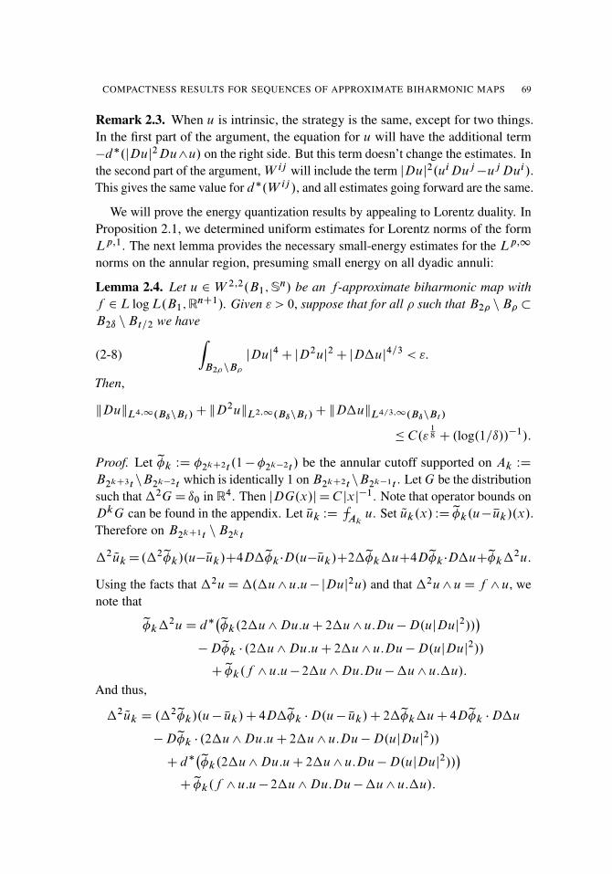
COMPACTNESS RESULTS FOR SEQUENCES OF APPROXIMATE BIHARMONIC MAPS 69
Remark 2.3. When u is intrinsic, the strategy is the same, except for two things.In the first part of the argument, the equation for u will have the additional term�d�.jDuj2Du^u/ on the right side. But this term doesn’t change the estimates. Inthe second part of the argument, W ij will include the term jDuj2.uiDuj�uj Dui/.This gives the same value for d�.W ij /, and all estimates going forward are the same.
We will prove the energy quantization results by appealing to Lorentz duality. InProposition 2.1, we determined uniform estimates for Lorentz norms of the formLp;1. The next lemma provides the necessary small-energy estimates for the Lp;1
norms on the annular region, presuming small energy on all dyadic annuli:
Lemma 2.4. Let u 2 W 2;2.B1;Sn/ be an f-approximate biharmonic map with
f 2L log L.B1;RnC1/. Given " > 0, suppose that for all � such that B2� nB� �
B2ı nBt=2 we have
(2-8)Z
B2�nB�
jDuj4CjD2uj2CjD�uj4=3 < ":
Then,
kDukL4;1.BınBt /CkD2ukL2;1.BınBt /
CkD�ukL4=3;1.BınBt /
� C."18 C .log.1=ı//�1/:
Proof. Let z�k WD �2kC2t .1� �2k�2t / be the annular cutoff supported on Ak WD
B2kC3t nB2k�2t which is identically 1 on B2kC2t nB2k�1t . Let G be the distributionsuch that�2GD ı0 in R4. Then jDG.x/j DC jxj�1. Note that operator bounds onDkG can be found in the appendix. Let uk WD �
RAk
u. Set Quk.x/ WD z�k.u�uk/.x/.Therefore on B2kC1t nB2k t
�2QukD .�
2z�k/.u�uk/C4D�z�k �D.u�uk/C2�z�k�uC4Dz�k �D�uCz�k�2u:
Using the facts that �2uD�.�u^u:u� jDuj2u/ and that �2u^uD f ^u, wenote that
z�k�2uD d�
�z�k.2�u^Du:uC 2�u^u:Du�D.ujDuj2//
��Dz�k � .2�u^Du:uC 2�u^u:Du�D.ujDuj2//
C z�k.f ^u:u� 2�u^Du:Du��u^u:�u/:
And thus,
�2Quk D .�
2z�k/.u�uk/C 4D�z�k �D.u�uk/C 2�z�k�uC 4Dz�k �D�u
�Dz�k � .2�u^Du:uC 2�u^u:Du�D.ujDuj2//
C d��z�k.2�u^Du:uC 2�u^u:Du�D.ujDuj2//
�C z�k.f ^u:u� 2�u^Du:Du��u^u:�u/:

70 CHRISTINE BREINER AND TOBIAS LAMM
For ease of notation, we let Ik denote the first four terms above, and IIk ; IIIk ; IVk
denote the last three terms, respectively. Then on each B2kC1t nB2k t
jDu.x/j D jD.z�k.u�uk//.x/j D j�2G �D.z�k.u�uk//.x/j
D jDG ��2.z�k.u�uk//.x/j D jDG � .Ik C IIk C IIIk C IVk/.x/j:
We consider each of these estimates separately. First, note that
jDG � Ik.x/j
� C
ˇZ.B
2kC3tnB
2kC2t/[.B
2k�1tnB
2k�2t/
1
jx�yj
��.2k t/�4.u�uk/C .2
k t/�3D.u�uk/C .2k t/�2�uC .2k t/�1D�u
�dy
ˇ� C
ˇZAk
.2k t/�1�.2k t/�4.u�uk/C .2
k t/�3Du
C .2k t/�2�uC .2k t/�1D�u�
dy
ˇ� C
ZAk
.2k t/�4jDujC .2k t/�3
jD2ujC .2k t/�2jD�uj
� C.2k t/�1.kDukL4 CkD2ukL2 CkD�ukL4=3/
� C."1=4C "1=2
C "3=4/jxj�1:
Using the same ideas as previously, we bound
jDG � IIk.x/j
� C.2k t/�2
ZAk
j2�u^Du:uC 2�u^u:Du�D.ujDuj2/j
� C.2k t/�1k2�u^Du:uC 2�u^u:Du�D.ujDuj2/kL4=3.Ak/
� C.2k t/�1.kD2ukL2kDukL4 CkDuk3L4/
� C."1=8C "3=4/jxj�1:
Using the estimates from the appendix, we note that
kDG � IIIk kL4;1.Ak/
� CkD2G� z�k.2�u^Du:uC 2�u^u:Du�D.ujDuj2/kL4;1.Ak/
� Ckz�k.2�u^Du:uC 2�u^u:Du�D.ujDuj2//kL4=3.Ak/
and
kDG � IVk kL4;1.Ak/� Ckz�k.f ^u:u� 2�u^Du:Du��u^u:�u/kL1.Ak/
:

COMPACTNESS RESULTS FOR SEQUENCES OF APPROXIMATE BIHARMONIC MAPS 71
Thus
jfx W jDG � .IIIk C IVk/.x/j> �gj
� ��4kDG�.IIIk C IVk/k
4L4;1.R4/
� C��4�kz�k.f ^u:u�2�u^Du:Du��u^u:�u/k4
L1.Ak/
Ckz�k.2�u^Du:uC2�u^u:Du�D.ujDuj2//k4L4=3.Ak/
�� C��4
��Zz�k jD
2uj2�2Z
z�k jDuj4C
�Zz�k jDuj4
�3�CC��4
kz�k.f ^u:u�2�u^Du:Du��u^u:�u/k4L1.Ak/
:
Thus, if ı D 2M t , then (letting Sk WD B2kC1t nB2k t for ease of notation)
jfx 2 Bı nBt W jDu.x/j> 3�gj
�
M�1XkD0
jfx 2 Sk W jDu.x/j> 3�gj
�
M�1XkD0
jfx 2 Sk W jDG � Ik j> �gjC
M�1XkD0
jfx 2 Sk W jDG � IIk j> �gj
C
M�1XkD0
jfx 2 Sk W jDG � .IIIk C IVk/j> �gj
�
M�1XkD0
jfjDG � .IIIk C IVk/j> �gjC
ˇ�x 2 B1 W C
"18
jxj> �
�ˇ
� C��4
"
12 C
M�1XkD0
kz�k.f ^u:u/k4L1.Ak/
C
M�1XkD0
��Zz�k jD
2uj2�4
C
�Zz�k jDuj4
�4
C
�Zz�k jDuj4
�3
C
�Zz�k jDuj4
�2�!� C��4."
12 C .log.1=ı//�4
kf k4L log L.B2ı/C "2/:
For the estimate on kf ^ u:ukL1 we use Lemma A.2, and for the rest of theL1 estimate we just use Cauchy–Schwarz. This proves the estimate for Du. Theestimates for D2u and D�u work in much the same way. In the case of D2u,the terms like IIIk and IVk require the fact that D3G WL4=3!L2;1 and D2G W
L1! L2;1 are bounded operators, where the operation is convolution. For theterm D�u we observe that D3G WL1!L4=3;1 and D4G WL4=3!L4=3;1 arealso bounded operators. �

72 CHRISTINE BREINER AND TOBIAS LAMM
3. Energy quantization — proof of Theorem 1.2
We now determine a weak convergence result which will give small-energy com-pactness and help us complete the proof of the energy quantization. We followthe ideas of [Li and Zhu 2011; Sharp and Topping 2013], which in turn follow thearguments of [Evans 1990], with appropriate minor modifications. Throughout thislemma and its proof, we consider a measurable function f as both a function and aRadon measure.
Lemma 3.1. Suppose fVkg � W 1;4=3.B1/ is a bounded sequence in B1 � R4.Then there exist at most countable fxig � B1 and fai > 0g with
Pi ai <1 and
V 2W 1;4=3.B1/ such that, after passing to a subsequence,
V 2k * V 2
C
Xi
aiıxi
weakly as measures.
Proof. As W 1;4=3 embeds continuously into L2 in four dimensions, after taking asubsequence, by Rellich compactness there exists some V 2L2 such that Vk ! V
strongly in Lp for 1 � p < 2 and Vk * V weakly in L2. Moreover, sincefDVkg is uniformly bounded in L4=3, it follows that DVk *f 2L4=3 and f isnecessarily DV .
Set gk WD Vk �V . Then gk 2L2 and Dgk 2L4=3 with uniform bounds. Thus,in the weak-� topology, both jDgk j
4=3 and g2k
converge to nonnegative Radon mea-sures with finite total mass. (We denote this space by M.B/). Then g2
k*� 2M.B/
and jDgk j4=3 * � 2 M.B/ where �, � are both nonnegative. Now consider
�2C 10.B1/, and observe that the Sobolev embedding of W 1;4=3 into L2 implies that�Z
.�gk/2 dx
�12
� C
�ZjD.�gk/j
43 dx
�34
:
Taking k!1 and noting that gk ! 0 in L4=3, we use the weak convergence toobserve that Z
�2 d� � C
�Zj�j
43 d�
�32
:
Let � approximate �Br .x/ for Br .x/� B1. Then
�.Br .x//� C��.Br .x//
� 32 :
By standard results on the differentiation of measures (see [Evans and Gariepy1992, Section 1.6]), for any Borel set E
�.E/D
ZE
D�� d�;

COMPACTNESS RESULTS FOR SEQUENCES OF APPROXIMATE BIHARMONIC MAPS 73
where
D��.x/D limr!0
�.Br .x//
�.Br .x//for �-a.e. x 2 R4:
Now, as � is a finite, nonnegative Radon measure, there exist at most countablymany xi 2B1 such that �.fxig/ > 0. Moreover, for all x 2B such that �.fxg/D 0,we note that
D��.x/D limr!0
�.Br .x//
�.Br .x//� C lim
r!0�.Br .x//
12 D 0:
For every xj such that �.fxj g/ > 0, set aj DD��.xj /�.fxj g/. Then
�.E/D
ZE
D�� d�DX
fj Wxj2Eg
aj or � DX
j
ajıxj :
Since g2k*� as measures, for � 2 C 0
0.B1/,X
j
aj�.xj /D limk!1
ZB1
g2k� dx D lim
k!1
ZB1
.Vk �V /2 dx:
Since .Vk �V /2D V 2k�V 2C2V .V �Vk/ and V �Vk D gk * 0 in L2, we have
the result. �Corollary 3.2. For fVkg as in Lemma 3.1, if
(3-1) limr!0
lim supk!1
kVkkL2.Br .x//D 0
for all x 2 B, thenVk ! V strongly in L2
loc.B/:
Proof. Notice the condition (3-1) implies that jVk j2 * jV j2 weakly as bounded
Radon measures. Then, by [Evans and Gariepy 1992, Section 1.9], for any Br .x/�
B1, we have kVkkL2.Br .x//!kV kL2.Br .x//
strongly for all Br .x/� B1. Then,again using the fact that .Vk �V /2 D V 2
k�V 2C 2V .V �Vk/ andZ
Br .x/
V 2k �V 2 dxC
ZBr .x/
2V .V �Vk/ dx! 0 as k!1;
we conclude that Vk ! V strongly in L2loc.B1/. �
We now use the energy estimates of Proposition 2.1 to prove a small-energycompactness result:
Lemma 3.3. Let uk be a sequence of fk-approximate biharmonic maps in B2 withfk 2L log L.B2/ satisfying (1-1). There exists "0 > 0 such that if
kDukkL4.B2/CkD2ukkL2.B2/
< "0;
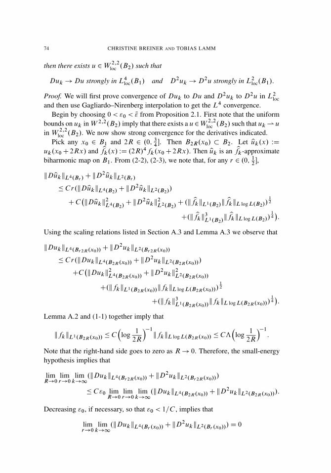
74 CHRISTINE BREINER AND TOBIAS LAMM
then there exists u 2W2;2
loc .B2/ such that
Duk !Du strongly in L4loc.B1/ and D2uk !D2u strongly in L2
loc.B1/:
Proof. We will first prove convergence of Duk to Du and D2uk to D2u in L2loc
and then use Gagliardo–Nirenberg interpolation to get the L4 convergence.Begin by choosing 0< "0 < Q" from Proposition 2.1. First note that the uniform
bounds on uk in W 2;2.B2/ imply that there exists a u2W2;2
loc .B2/ such that uk *u
in W2;2
loc .B2/. We now show strong convergence for the derivatives indicated.Pick any x0 2 B1 and 2R 2 .0; 3
4�. Then B2R.x0/ � B2. Let yuk.x/ WD
uk.x0C2Rx/ and yfk.x/ WD .2R/4fk.x0C2Rx/. Then yuk is an yfk-approximatebiharmonic map on B1. From (2-2), (2-3), we note that, for any r 2 .0; 1
2�,
kDyukkL4.Br /CkD2
yukkL2.Br /
� C r.kDyukkL4.B2/CkD2
yukkL2.B2//
CC�kDyukk
2L4.B2/
CkD2yukk
2L2.B2/
C .k yfkkL1.B2/k yfkkL log L.B2//
12
C.k yfkk3L1.B2/
k yfkkL log L.B2//14
�:
Using the scaling relations listed in Section A.3 and Lemma A.3 we observe that
kDukkL4.Br 2R.x0//CkD2ukkL2.Br 2R.x0//
� C r.kDukkL4.B2R.x0//CkD2ukkL2.B2R.x0//
/
CC�kDukk
2L4.B2R.x0//
CkD2ukk2L2.B2R.x0//
C.kfkkL1.B2R.x0//kfkkL log L.B2R.x0///
12
C.kfkk3L1.B2R.x0//
kfkkL log L.B2R.x0///14
�:
Lemma A.2 and (1-1) together imply that
kfkkL1.B2R.x0//� C
�log 1
2R
��1kfkkL log L.B2R.x0// � Cƒ
�log 1
2R
��1:
Note that the right-hand side goes to zero as R! 0. Therefore, the small-energyhypothesis implies that
limR!0
limr!0
limk!1
.kDukkL4.Br 2R.x0//CkD2ukkL2.Br 2R.x0//
/
� C "0 limR!0
limr!0
limk!1
.kDukkL4.B2R.x0//CkD2ukkL2.B2R.x0//
/:
Decreasing "0, if necessary, so that "0 < 1=C , implies that
limr!0
limk!1
.kDukkL4.Br .x0//CkD2ukkL2.Br .x0//
/D 0

COMPACTNESS RESULTS FOR SEQUENCES OF APPROXIMATE BIHARMONIC MAPS 75
for all x0 2 B1. Let Vk DD2uk and V DD2u. Since Vk * V weakly in L2 asmeasures and Vk satisfies the hypotheses of Lemma 3.1 and Corollary 3.2 on B1,Vk ! V strongly in L2
loc.B1/.Since Duk *Du weakly as measures in L2.B2/ and
limr!0
limk!1
kDukkL2.Br .x0//� lim
r!0lim
k!1rkDukkL4.Br .x0//
D 0
for all x0 2 B1, Corollary 3.2 again implies that Duk !Du strongly in L2loc.B1/.
Now, for any Br .x/� B1, we consider the functions
wk WD .uk �u/� �
ZBr .x/
.uk �u/:
Then, Dwk D D.uk � u/ and D2wk D D2.uk � u/. We apply the Gagliardo–Nirenberg interpolation inequality for wk and then the Poincaré inequality for theL2 estimates on wk to conclude that
kDwkkL4.Br .x//� CkD2wkkL2.Br .x//
kDwkkL2.Br .x//CCkDwkkL2.Br .x//
:
Then, using the strong convergence of D2uk ! Du in L2loc and Duk ! Du in
L2loc, we conclude Duk !Du in L4
loc.B1/. �
Finally, we prove the energy quantization result under the presumption of onebubble at the origin.
Proposition 3.4. Let fk 2 L log L.B1;RnC1/, and let uk 2 W 2;2.B1;S
n/ be asequence of fk-approximate biharmonic maps with bounded energy such that
uk ! u in W2;2
loc .B1 n f0g;Sn/;
Quk.x/ WD uk.�kx/! !.x/ in W2;2
loc .R4;Sn/:
Presume further that ! is the only “bubble” at the origin. Let
Ak.ı;R/ WD fx W �kR� jxj � ıg:
Then
limR!1
limı!0
limk!1
�kD2ukkL2.Ak.ı;R//
CkDukkL4.Ak.ı;R//
CkD�ukkL4=3.Ak.ı;R//
�D 0:
The proposition also holds if uk is a sequence of fk-approximate intrinsic bihar-monic maps.

76 CHRISTINE BREINER AND TOBIAS LAMM
Proof. We first prove that for any " > 0 there exists K sufficiently large and ı smallso that, for all k �K and �k > 0 such that B4�k
nB�k=2 �Ak.ı;R/,
(3-2) kD2ukkL2.B2�knB�k
/CkDukkL4.B2�knB�k
/CkD�ukkL4=3.B2�knB�k
/
< ":
Since f0g is the only point of energy concentration, the strong convergence ofD2uk ! D2u in L2 and Duk ! Du in L4 implies that for any " > 0 and anym 2 ZC and ı sufficiently small, there exists K WDK.m/ sufficiently large suchthat, for all k �K.m/,
(3-3) kD2ukkL2.B2ınBı2�m�1 /
CkDukkL4.B2ınBı2�m�1 /
�"
C�mC3:
Here C is an appropriately large constant determined by the bounds of Proposition 2.1and � is the number of balls of radius r=32 needed to cover Br nBr=2. By (2-4),for any x 2 B2ı nBı2�m�1 and 0< r < ı2�m�1,
(3-4) kD�ukkL4=3.Br=32.x//� C
�kD2ukkL2.Br=2.x//
CkDukkL4.Br=2.x//
Ckfkk1=4
L1.Br=2.x//kfkk
3=4
L log L.Br=2.x//
�Since Lemma A.2 and (1-1) imply that
(3-5) kfkkL1.Br=2.x//� C
�log 1
r
��1kfkkL log L.Br=2.x//;
for sufficiently small ı, (3-3), (3-4), and (3-5) together imply that for k �K.m/
(3-6) kD�ukkL4=3.B2ınBı2�m�1 /CkDukkL4.B2ınBı2�m�1 /
CkD2ukkL2.B2ınBı2�m�1 /�
12":
A similar argument (perhaps requiring a larger K) implies that
(3-7) kD�ukkL4=3.B2m�k RnB�k R/CkDukkL4.B2m�k RnB�k R/
CkD2ukkL2.B2m�k RnB�k R/�
12":
Now suppose there exists a sequence tk with �kR< tk < ı such that
kD2ukkL2.B2tknBtk
/CkDukkL4.B2tknBtk
/CkD�ukkL4=3.B2tknBtk
/ � ":
By (3-6) and (3-7), tk!0 and Bı=tknB�kR=tk
!R4nf0g. Define vk.x/Duk.tkx/
and Qfk.x/ WD t4kfk.tkx/. Then vk is an Qfk-approximate biharmonic map, defined on
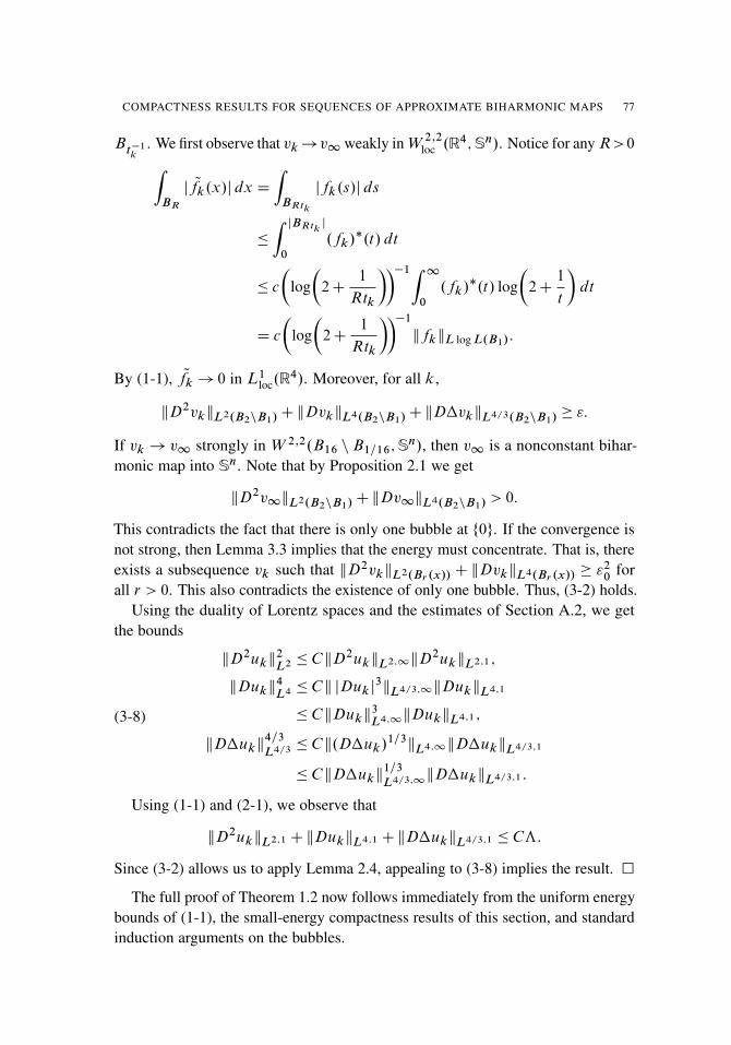
COMPACTNESS RESULTS FOR SEQUENCES OF APPROXIMATE BIHARMONIC MAPS 77
Bt�1k
. We first observe that vk!v1 weakly in W2;2
loc .R4;Sn/. Notice for any R>0Z
BR
j Qfk.x/j dx D
ZBRtk
jfk.s/j ds
�
Z jBRtkj
0
.fk/�.t/ dt
� c
�log�
2C1
Rtk
���1Z 10
.fk/�.t/ log
�2C
1
t
�dt
D c
�log�
2C1
Rtk
���1
kfkkL log L.B1/:
By (1-1), Qfk ! 0 in L1loc.R
4/. Moreover, for all k,
kD2vkkL2.B2nB1/CkDvkkL4.B2nB1/
CkD�vkkL4=3.B2nB1/� ":
If vk ! v1 strongly in W 2;2.B16 nB1=16;Sn/, then v1 is a nonconstant bihar-
monic map into Sn. Note that by Proposition 2.1 we get
kD2v1kL2.B2nB1/CkDv1kL4.B2nB1/
> 0:
This contradicts the fact that there is only one bubble at f0g. If the convergence isnot strong, then Lemma 3.3 implies that the energy must concentrate. That is, thereexists a subsequence vk such that kD2vkkL2.Br .x//
CkDvkkL4.Br .x//� "2
0for
all r > 0. This also contradicts the existence of only one bubble. Thus, (3-2) holds.Using the duality of Lorentz spaces and the estimates of Section A.2, we get
the bounds
(3-8)
kD2ukk2L2 � CkD2ukkL2;1kD2ukkL2;1 ;
kDukk4L4 � Ck jDuk j
3kL4=3;1kDukkL4;1
� CkDukk3L4;1kDukkL4;1 ;
kD�ukk4=3
L4=3 � Ck.D�uk/1=3kL4;1kD�ukkL4=3;1
� CkD�ukk1=3
L4=3;1kD�ukkL4=3;1 :
Using (1-1) and (2-1), we observe that
kD2ukkL2;1 CkDukkL4;1 CkD�ukkL4=3;1 � Cƒ:
Since (3-2) allows us to apply Lemma 2.4, appealing to (3-8) implies the result. �
The full proof of Theorem 1.2 now follows immediately from the uniform energybounds of (1-1), the small-energy compactness results of this section, and standardinduction arguments on the bubbles.

78 CHRISTINE BREINER AND TOBIAS LAMM
4. Oscillation bounds
The proof of the following oscillation lemma will constitute the work of this section:
Lemma 4.1. Let u 2 W 2;2.B1;Sn/ be an f -approximate biharmonic map for
f 2L log L.B1;RnC1/ with
kD2ukL2.B1/CkDukL4.B1/
Ckf kL log L.B1/ �ƒ<1:
Then for 0< 2t < ı=2< 1=16,
supx;y2Bı=2nB2t
ju.x/�u.y/j
� C�kD2ukL2.B2ınBt /
CkDukL4.B2ınBt /Ckf kL log L.B2ı/
CkD�ukL4=3.B2ınBt /CkD�ukL4=3;1.B2tnBt /
CjB4ıj�:
The lemma also holds if u is an f -approximate intrinsic biharmonic map.
Consider the map u1 WB1! RnC1 such that u1.x/D bCAx, where b 2 RnC1
and A is an .nC 1/� 4 matrix with
A WD �
ZB2tnBt
Du and b WD �
ZB2tnBt
.u.x/�Ax/ dVol.x/:
Then by construction
�
ZB2tnBt
u�u1 D 0; �
ZB2tnBt
Du�Du1 D 0; Dku1 � 0 for all k � 2:
Set wD .1��t /.u�u1/. Let w1 WB1!RnC1 such that w1.x/DmCN x, where
N WD �
ZBınBı=2
Dw and m WD �
ZBınBı=2
.w.x/�N x/ dVol.x/:
Let zw D .w�w1/�ı=2, so zw Dw�w1 on Bı=2 and the support of zw is containedin Bı.
By definition,
supx;y2Bı=2nB2t
ju.x/�u.y/j D supx;y2Bı=2nB2t
jw.x/�w.y/Cu1.x/�u1.y/j
D supx;y2Bı=2nB2t
j. zwCu1Cw1/.x/�. zwCu1Cw1/.y/j
� 2 supx2Bı=2nB2t
j zw.x/� zw.0/C.ACN /xj:
We first observe that, outside of B2t , wD u�u1 so the definition of N implies that
ACN DAC �
ZBınBı=2
Du� �
ZBınBı=2
AD �
ZBınBı=2
Du:

COMPACTNESS RESULTS FOR SEQUENCES OF APPROXIMATE BIHARMONIC MAPS 79
Thus, for x 2 Bı=2, Hölder’s inequality implies that
j.ACN /xj � Cı�3
ZBınBı=2
jDuj � CkDukL4.BınBı=2/:
As before, let G be the distribution in R4 such that �2G D ı0. Then G.x/ D
C log jxj, and recall that DG 2L4;1.R4/. It is enough to show that:
Claim 4.2.ˇzw.x/� �
ZR4
zw
ˇ� CkD� zwkL4=3;1.R4/:
Since all of the above quantities are translation-invariant, we may assume x D 0.Then ˇ
zw.0/� �
Zzw
ˇD
ˇZR4
�2G.y/
�zw.y/� �
Zzw
�dV .y/
ˇD
ˇZR4
DG.y/D� zw.y/ dV .y/
ˇ� CkDGkL4;1.R4/kD� zwkL4=3;1.R4/:
Using the definition of zw,
kD� zwkL4=3;1.R4/
� Ck.ı�3jw�w1jC ı
�2jD.w�w1/jC ı
�1jD2wj/kL4=3;1.BınBı=2/
CCkD�wkL4=3;1.Bı/:
Interpolation techniques and Poincaré’s inequality imply that
kı�3.w�w1/kL4=3;1.BınBı=2/� Ckı�2D.w�w1/kL4=3;1.BınBı=2/
� Ckı�1D2wkL4=3;1.BınBı=2/:
Moreover, the embedding theorems for Lorentz spaces imply that
kı�1D2wkL4=3;1.BınBı=2/� CkD2wkL2.BınBı=2/
:
Therefore,
(4-1) kD� zwkL4=3;1.R4/ � CkD2wkL2.BınBı=2/CCkD�wkL4=3;1.Bı/
:
Since D2w DD2u on Bı nB2t , we conclude that
(4-2) oscBı=2nB2tu
� C.kD�wkL4=3;1.Bı/CkD2ukL2.BınBı=2/
CkDukL4.BınBı=2//:
The remainder of the proof will be devoted to bounding the D�w term.We define ˇ DD�w^u��w^Du. Then
ˇijWD uj D�wi
�uiD�wj��wiDuj
C�wj Dui2�1R4

80 CHRISTINE BREINER AND TOBIAS LAMM
for i; j D 1; : : : ; nC 1. By definition ˇ DD�u^ u��u^Du in Bı nB2t andthus d�ˇ D f ^u in Bı nB2t . We will require an L4=3 bound for ˇ, and to thatend note that
(4-3) kˇkL4=3.B2ı/� C.kD�wkL4=3.B2ı/
Ck�w^DukL4=3.B2ı//
� C.kD�wkL4=3.B2ı/Ck�wkL2.B2ı/
kDukL4.B2ı//
� C.kD�ukL4=3.B2ınBt /CkD2ukL2.B2ınBt /
/:
For the last inequality, kDukL4.B2ı/is bounded and is absorbed into the constant.
In addition, we use the definition of w and repeated applications of Poincaré andHölder to determine
kD�wkL4=3.B2ı/� C.kD2ukL2.B2tnBt /
Ck.1��t /D�ukL4=3.B2ı//;
k�wkL2.B2ı/� CkD2ukL2.B2ınBt /
:
Set
WD d�.D�.w�u/^u��.w�u/^Du/:
Then
d�ˇ D f ^uC ; dˇ D�2D�w^Du;
�ˇ D .dd�C d�d/ˇ D d.f ^uC /C d�.�2D�w^Du/:
We consider a decomposition ˇij DH ij Cd‰ij Cd�ˆij for each component ˇij ,where H ij is a harmonic 1-form and ˆ;‰ satisfy appropriate partial differentialequations. Our objective is to bound kD�wkL4=3;1 by kˇkL4=3;1 , and to that endwe determine such bounds for d‰, d�ˆ, and H .
Remark 4.3. For the intrinsic case, we modify a few definitions. Let ˇI WD
ˇC2jDuj2DwI^u, wherewI D .1��t /.u�d/ and d WD �R
B2tnBtu. Using the def-
inition ofwI , we get the bound kˇIkL4=3.B2ı/�kˇkL4=3.B2ı/
CCkDukL4.B2ınBt /
by using Hölder’s inequality and Poincaré’s inequality. We then define I WD
C d�.2jDuj2D.wI �u/^u/, and thus
d�ˇI D f ^uC I and dˇI D dˇCD.jDuj2/DwI ^u� jDuj2DwI ^Du:
We now continue with the proof for the extrinsic case:
Proposition 4.4. Let ‰ij be a function on B2ı satisfying��‰ij D f iuj �f j ui C ij in B2ı;
‰ij D 0 on @B2ı:
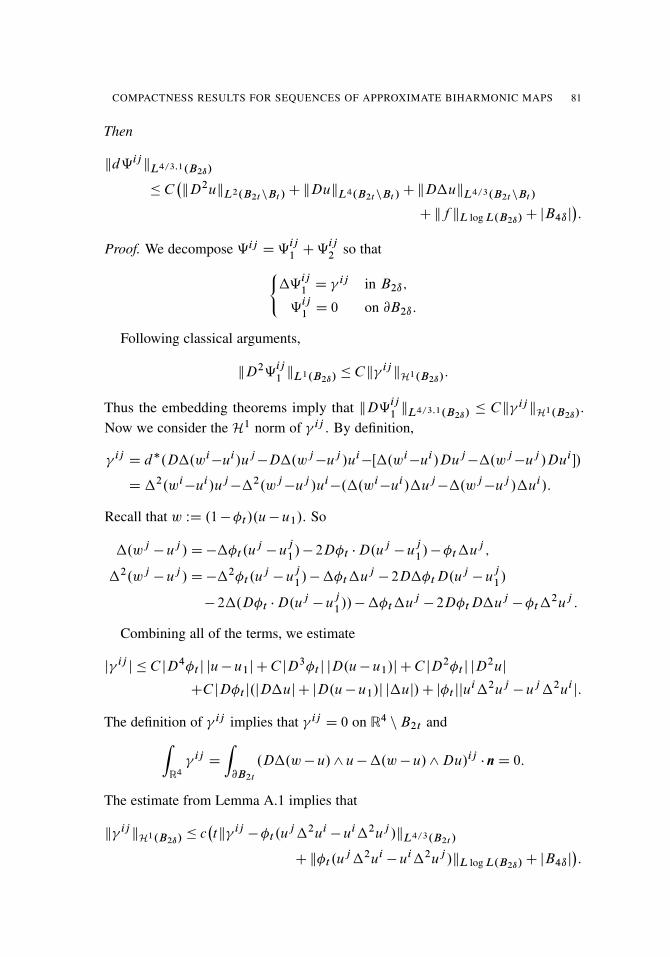
COMPACTNESS RESULTS FOR SEQUENCES OF APPROXIMATE BIHARMONIC MAPS 81
Then
kd‰ijkL4=3;1.B2ı/
� C�kD2ukL2.B2tnBt /
CkDukL4.B2tnBt /CkD�ukL4=3.B2tnBt /
Ckf kL log L.B2ı/CjB4ıj�:
Proof. We decompose ‰ij D‰ij1C‰
ij2
so that(�‰
ij1D ij in B2ı;
‰ij1D 0 on @B2ı:
Following classical arguments,
kD2‰ij1kL1.B2ı/
� Ck ijkH1.B2ı/
:
Thus the embedding theorems imply that kD‰ij1kL4=3;1.B2ı/
� Ck ijkH1.B2ı/.
Now we consider the H1 norm of ij . By definition,
ijD d�.D�.wi
�ui/uj�D�.wj
�uj /ui�Œ�.wi
�ui/Duj��.wj
�uj /Dui �/
D�2.wi�ui/uj
��2.wj�uj /ui
�.�.wi�ui/�uj
��.wj�uj /�ui/:
Recall that w WD .1��t /.u�u1/. So
�.wj�uj /D���t .u
j�u
j1/� 2D�t �D.u
j�u
j1/��t�uj ;
�2.wj�uj /D��2�t .u
j�u
j1/���t�uj
� 2D��tD.uj�u
j1/
� 2�.D�t �D.uj�u
j1//���t�uj
� 2D�tD�uj��t�
2uj :
Combining all of the terms, we estimate
j ijj � C jD4�t j ju�u1jCC jD3�t j jD.u�u1/jCC jD2�t j jD
2uj
CC jD�t j.jD�ujC jD.u�u1/j j�uj/Cj�t jjui�2uj
�uj�2uij:
The definition of ij implies that ij D 0 on R4 nB2t andZR4
ijD
Z@B2t
.D�.w�u/^u��.w�u/^Du/ij �nD 0:
The estimate from Lemma A.1 implies that
k ijkH1.B2ı/
� c�tk ij
��t .uj�2ui
�ui�2uj /kL4=3.B2t /
Ck�t .uj�2ui
�ui�2uj /kL log L.B2ı/CjB4ıj�:
82 CHRISTINE BREINER AND TOBIAS LAMM
Repeating techniques used previously, we bound the first three terms of j ij j:
t�4ku�u1kL4=3.B2tnBt /
� C t�3kD.u�u1/kL4=3.B2tnBt /
� C t�2kD2ukL4=3.B2tnBt /
� C t�1kD2ukL2.B2tnBt /
:
We will preserve the term
t�1kD�ukL4=3.B2tnBt /
;
as our energy quantization result implies that this term will vanish when taking limits.Hölder’s inequality and the fact that kD.u�u1/kL4.B2tnBt /
� CkDukL4.B2tnBt /
imply that
kD.u�u1/�ukL4=3.B2tnBt /� CkD.u�u1/kL4.B2tnBt /
kD2ukL2.B2tnBt /
� CkD2ukL2.B2tnBt /:
For the last term, since u is an f -approximate biharmonic map into Sn,
k�t .�2u^u/kL log L.B2ı/ � kf ^ukL log L.B2ı/ � kf kL log L.B2ı/:
All of the above estimates imply that
k ijkH1.B2ı/
� C�kD2ukL2.B2tnBt /
CkDukL4.B2tnBt /
CkD�ukL4=3.B2tnBt /Ckf kL log L.B2ı/CjB4ıj
�:
Finally, consider (�‰
ij2D f iuj �uif j in B2ı;
‰ij2D 0 on @B2ı:
Then classical results give k‰ij2kW 2;1.B2ı/
� Ckf kH1.B2ı/� Ckf kL log L.B2ı/.
Thuskd‰
ij2kW 1;1.B2ı/
� Ckf kL log L.B2ı/;
and the embedding theorems in R4 imply that
kd‰ij2kL4=3;1.B2ı/
� Ckf kL log L.B2ı/: �
Remark 4.5. For the intrinsic case, we define
I D Cd�.2jDuj2D.wI �u/^u/
D �2�td�.jDuj2Du^u/C2jDuj2.��t .d�u/^u�D�t �Du^.dCu//
C2DjDuj2 �D�t .d�u/^u:
We bound k IkH1 by making some observations: First, �2�td�.jDuj2Du^ u/
is added to the term ��t�2u ^ u that appears in the expansion of . We then
make the substitution ��tf ^u as in the extrinsic case. Second, using Poincaré’s
COMPACTNESS RESULTS FOR SEQUENCES OF APPROXIMATE BIHARMONIC MAPS 83
inequality, Hölder’s inequality, and the global energy bound for u, the L4=3 norm ofwhat remains is bounded by C t�1.kDukL4.B2tnBt /
CkD2ukL2.B2tnBt //. Finally,
observe that, by construction, I is supported on B2t andR
R4 I D0, so the estimateused for k kH1 still applies.
Proposition 4.6. Let ˆij 2�2R4 be the solution to the system��ˆij D�2.D�wiDuj �D�wj Dui/ in B2ı;
ˆij D 0 on @B2ı:
Then
(4-4) kd�ˆijkL4=3;1.B2ı/
� C.kD2ukL2.B2tnBt /CkD�ukL4=3.B2ınBt /
/:
Proof. Using the same techniques and estimates as in the previous proposition,we note that
kdˆijkL4=3;1.B2ı/
� CkD�w^DukH1.B2ı/
� CkD�wkL4=3.B2ı/kDukL4.B2ı/
� C.kD2ukL2.B2tnBt /CkD�ukL4=3.B2ınBt /
/: �
Remark 4.7. In the intrinsic setting the steps of the proof are the same, though theequation for�ˆij
Iincludes the terms D.jDuj2/DwI ^u�jDuj2DwI ^Du. Since
kDwIkL4.B2ı/�CkDukL4.B2ınBt /
, one can quickly show the intrinsic bound hasthe form
kd�ˆIkL4=3;1.B2ı/� kd�ˆkL4=3;1.B2ı/
CCkDukL4.B2ınBt /:
Now consider the harmonic 1-form
H ijD ˇij
� d�ˆij� d‰ij :
Propositions 4.4 and 4.6, along with (4-3), imply that
kHkL4=3.B2ı/� kˇkL4=3.B2ı/
Ckd�ˆkL4=3.B2ı/Ckd‰kL4=3.B2ı/
� C�kD2ukL2.B2ınBt /
CkDukL4.B2ınBt /
CkD�ukL4=3.B2ınBt /Ckf kL log L.B2ı/CjB4ıj
�:
The mean value property and Hölder’s inequality together imply that
kH ijkC 0.Bı/
�C
ı3
�kD2ukL2.B2ınBt /
CkDukL4.B2ınBt /
CkD�ukL4=3.B2ınBt /Ckf kL log L.B2ı/CjB4ıj
�:
Moreover, a straightforward calculation implies that
kH ijkL4=3;1.Bı/
� Cı3kH ij
kC 0.Bı/:

84 CHRISTINE BREINER AND TOBIAS LAMM
Thus,
kˇkL4=3;1.Bı/� C
�kD2ukL2.B2ınBt /
CkDukL4.B2ınBt /
CkD�ukL4=3.B2ınBt /Ckf kL log L.B2ı/CjB4ıj
�:
Using the appropriate harmonic 1-form HI , we produce an identical estimate for ˇI .We now use the definitions ofw and ˇ to determine a bound on kD�wkL4=3;1.Bı/
.First we consider the function on B2t
kD�wkL4=3;1.B2t /
� kC.t�3ju�u1jC t�2
jD.u�u1/jC t�1jD2uj/kL4=3;1.B2tnBt /
Ck.1��t /D�ukL4=3;1.B2t /
� CkD2ukL2.B2tnBt /CCkD�ukL4=3;1.B2tnBt /
:
On Bı nB2t , w D u� u1 so D�w � D�u. We first decompose D�u intotangential and normal parts with tangency relative to the target manifold Sn. Then
D�uDD�uTCD�uN
DD�u^u:uChD�u;uiu:
Here we define hDv;ui WDP
i;k.@vk=@xi/u
k dxi . On Bı n B2t , D�u ^ u D
ˇC�u^Du, and thus
j.D�u/T j � jˇjC j�uj jDuj:
Since
hD�u;ui DDh�u;ui � h�u;Dui DD.d�hDu;ui � jDuj2/� h�u;Dui
D �DjDuj2� h�u;Dui;
we estimate
kD�wkL4=3;1.BınB2t /
� CkˇkL4=3;1.Bı/CCkD2ukL2.BınB2t /
kDukL4.BınB2t /
� C�kD2ukL2.B2ınBt /
CkDukL4.B2ınBt /CkD�ukL4=3.B2ınBt /
Ckf kL log L.B2ı/CjB4ıj�:
Thus,
kD�wkL4=3;1.Bı/� C.kD2ukL2.B2ınBt /
CkDukL4.B2ınBt /Ckf kL log L.B2ı/
CkD�ukL4=3;1.B2tnBt /CkD�ukL4=3.B2ınBt /
CjB4ıj/:
Inserting this inequality into (4-2) proves the oscillation lemma.
COMPACTNESS RESULTS FOR SEQUENCES OF APPROXIMATE BIHARMONIC MAPS 85
Remark 4.8. To complete the proof in the intrinsic case, observe that, on Bı nB2t ,D�w ^ uDD�u^ uD ˇC�u^DuC 2jDuj2Du^ u. This changes the L1
estimate for j.D�u/T j on Bı nB2t , but using embedding theorems for Lorentzspaces we note that the L4=3;1 estimate is unchanged.
5. No-neck property — proof of Theorem 1.3
The proof of the no-neck property now follows easily from combining the energyquantization and the oscillation bounds.
Proof. As we may use induction to deal with the case of multiple bubbles, weprove the theorem for one bubble. Let �k be such that Quk.x/ WD uk.�kx/ !
!.x/ 2W2;2
loc .R4;Sn/. Since each of the uk 2W 2;2.B1;S
n/ are fk-approximatebiharmonic maps with fk 2L log L.B1;R
nC1/ and have uniform energy bounds,Lemma 4.1 implies that
supx;y2Bı=2nB2�k R
juk.x/�uk.y/j
� C�kD2ukkL2.B2ınB�k R=2/
CkDukkL4.B2ınB�k R=2/
CkfkkL log L.B2ı/CkD�ukkL4=3;1.B�k RnB�k R=2/
CkD�ukkL4=3.B2ınB�k R=2/CjB4ıj
�:
Theorem 1.2 implies that
limı!0
limR!1
limk!1
�kD2ukkL2.B2ınB�k R=2/
CkDukkL4.B2ınB�k R=2/
CkD�ukkL4=3.B2ınB�k R=2/
�D 0:
Further, (2-1) and Hölder’s inequality imply that
kD�ukkL4=3;1.B�k RnB�k R=2/� C.kDukkL4.B2�k RnB�k R=4/
CkD2ukkL2..B2�k RnB�k R=4/CkfkkL log L.B2�k R//:
Since we presume the L log L norm of fk does not concentrate,
limı!0
limR!1
limk!1
kfkkL log L.B2ı/ D 0:
Therefore,
limı!0
limR!1
limk!1
kD�ukkL4=3;1.B�k RnB�k R=2/D 0:
Taking all of the estimates together implies that
limı!0
limR!1
limk!1
supx;y2Bı=2nB2�k R
juk.x/�uk.y/j D 0:
Thus, no neck occurs in the blowup. �

86 CHRISTINE BREINER AND TOBIAS LAMM
Remark 5.1. For fk 2 �.L/, we use the estimate
kfkkL log L.B2ı/
D
ZB2ı\fjfk j�ı�1g
jfk j log.2Cjfk j/ dxC
Zjfk j>ı�1
jfk j log.2Cjfk j/ dx
� Cı3 log.2C ı�1/C supt>ı�1
t log.2C t/
�.t/
Zjfk j>ı�1
�.jfk j/ dx
� Cı3 log.2C ı�1/C supt>ı�1
t log.2C t/
�.t/ƒ:
Since we presumed limt!1 �.t/=.t log t/D1, we determine
limı!0
supk
kfkkL log L.B2ı/ D 0:
Appendix: Necessary background
A.1. Hardy spaces, Lorentz spaces, L log L, and Orlicz spaces. Let
T WD fˆ 2 C1.R4/ W spt.ˆ/� B1; krˆkL1.R4/ � 1g:
For any ˆ 2 T , let ˆt .x/ WD t�4ˆ.x=t/. For each f 2L1.R4/, let
f�.x/D supˆ2T
supt>0
j.ˆt �f /.x/j:
Then f is in the Hardy space H1.R4/ if f� 2L1.R4/ and
kf kH1.R4/ D kf�kL1.R4/:
Thus, one has the continuous embedding H1 ,!L1.For a measurable function f W�!R, let f � denote the nonincreasing rearrange-
ment of jf j on Œ0; j�j/ such that
jfx 2� W jf .x/j � sgj D jft 2 .0; j�j/ W f �.t/� sgj:
Let
f ��.t/ WD1
t
Z t
0
f �.s/ ds:
For p 2 .1;1/, let
kf kLp;q D
�R10 t1=p�1f ��.t/ dt if q D 1;
supt>0 t1=pf ��.t/ if q D1:

COMPACTNESS RESULTS FOR SEQUENCES OF APPROXIMATE BIHARMONIC MAPS 87
We will also occasionally exploit the fact that one may understand kf kLp;1 byunderstanding instead its seminorm
kf k�Lp;1 WD sup�>0
�jfx W jf .x/j> �gj1=p:
We define the Banach spaces
Lp;qWD ff W kf kLp;q <1g:
The spaces Lp;1 and Lp;1 are examples of Lorentz spaces, and can be thought ofas interpolation spaces between the standard Lp spaces. For example, one observesthat the following embeddings are all continuous
Lr .B1/ ,!Lp;1.B1/ ,!Lp;p.B1/DLp.B1/ ,!Lp;1.B1/ ,!Lq.B1/
for all q < p < r [Hélein 1990].We define
L log L WD
�f W
Zjf .x/j log.2Cjf .x/j/ dx <1
�:
Since this is nonlinear, we will use the following seminorm which is equivalent tothe norm for L log L
kf kL log L WD
Zf �.t/ log
�2C
1
t
�dt:
We also note that Lp.B1/ ,!L log L.B1/ ,!L1.B1/ are continuous embeddingsfor all p > 1. Finally, we say f is in H1.B1/ if�
f � �
ZB1
f .x/ dx
��B12H1.R4/:
We record here the often-used estimate
(A-1) kf kH1.B1/� Ckf kL log L.B1/:
Finally, for any increasing function � W Œ0;1/! Œ0;1/we define the Orlicz space
�.L/ WD
�f W kf k�.L/ WD
Z�.jf j/ dx <1
�:
Examples include the Lp spaces for �.t/D tp and L log L when �.t/D t log.2Ct/.

88 CHRISTINE BREINER AND TOBIAS LAMM
A.2. Embeddings and estimates for Lorentz spaces. We will frequently use thefollowing facts about Lorentz spaces:
(1) Lp;q �Lp0;q0 continuously embeds into Lr;s for 1=pC 1=p0 � 1 where
1
rD
1
pC
1
p0and
1
sD
1
qC
1
q0;
withkfgkLr;s � Ckf kLp;qkgkLp0;q0 :
(2) For f 2L2 and g 2W 1;2,
kfgkL4=3;1 � Ckf kL2kgkW 1;2 :
(3) W 1;1.R4/ ,!L4=3;1.R4/ and W 1;2.R4/ ,!L4;2.R4/ are continuous embed-dings.
(4) L2;1 and L2;1 are dual spaces, as are L4;1, L4=3;1 and L4;1, L4=3;1.
(5) For all 0< p; r <1 and 0< q �1 (see [Grafakos 2008], Section 1.4.2),
kf rkLp;q D kf krLpr;qr :
(6) Let f 2 Lp;q.R4/ and g 2 Lp0;q0.R4/ with 1=p C 1=p0 > 1. Then h D
f � g 2 Lr;s.R4/ where 1=r D 1=pC 1=p0 � 1 and s is a number such that1=qC 1=q0 � 1=s. Moreover,
khkLr;s.R4/ � ckf kLp;q.R4/kgkLp0;q0 .R4/:
For a proof, see [Ziemer 1989].Let G be the distribution such that �2G D ı0. Then, D2G 2 L2;1.R4/
and D3G 2L4=3;1.R4/. Moreover, DG 2L4;1.R4/.Using (6), and considering D2G;D3G as operators by convolution, we
have:
(7) D2G W L4=3;1.R4/ ! L4;1.R4/ and D3G W L4=3;1.R4/ ! L2;1.R4/ arebounded operators.
A.3. Scaling and estimates for L log L and H1. We first prove an essential buttechnical lemma that is probably well known, though we have not found a referencein the literature. (We prove the lemma for our particular setting, though a moregeneral result is true.)
Lemma A.1. Let f D f1Cf2, where f1 2L4=3.BR/ and f2 2L log L.BR/, bea compactly supported function with spt.f / � BR and
RR4 f .x/ dx D 0. Then
f 2H1.BR/ and there exists C > 0 such that
(A-2) kf kH1.BR/� C.Rkf1kL4=3.BR/
Ckf2kL log L.BR/CjB2Rj/:
COMPACTNESS RESULTS FOR SEQUENCES OF APPROXIMATE BIHARMONIC MAPS 89
Proof. First note that
(A-3) kf�kL1 D
ZB2R
f�.x/ dxC
ZR4nB2R
f�.x/ dx:
Since f1 2L4=3.R4/ and f2 2L log L.R4/, we see that f 2L1loc.R
4/ and thereforef�.x/� cMf .x/ for every x 2 R4. Here Mf W R4! R is the maximal functiondefined by
Mf .x/D supr>0
1
jBr .x/j
ZBr .x/
jf .y/j dy:
Using the above, Hölder’s inequality and the estimates kMf1kL4=3 � ckf1kL4=3
and kMf2kL1.B2R/� ckf2kL log L.B2R/C cjB2Rj,
(A-4)Z
B2R
f�.x/ dx �cRk.f1/�kL4=3 Ck.f2/�kL1
�cRkMf1kL4=3 C ckMf2kL1
�cRkf1kL4=3 C ckf2kL log LC cjB2Rj:
Now we calculate for � 2 T and x 2 R4:
j�t ?f .x/j D
ˇZBR
�t .x�y/f .y/ dy
ˇD
ˇZBR
.�t .x�y/��t .x//f .y/ dy
ˇ� kr�tkL1
ZBR
jyjjf .y/j dy;
where we used the mean value theorem and the cancellation propertyR
R4 f .y/ dyD
0. Since kr�tkL1 � 1=t5, for t > 0, we estimate
(A-5) j�t ?f .x/j �R
t5
ZBR
jf .y/j dy
�cR2
t5kf1kL4=3 C
cR
t5kf2kL log L:
Assuming now that jxj � 2R, we can apply a technical result to get
(A-6) f�.x/D sup�2T
supt>jxj=2
j�t ?f .x/j �cR2
jxj5kf1kL4=3 C
cR
jxj5kf2kL log L:

90 CHRISTINE BREINER AND TOBIAS LAMM
Inserting (A-4) and (A-6) into (A-3), we conclude that
(A-7) kf�kL1 � cRkf1kL4=3 C ckf2kL log LC cjB2Rj
C .cR2kf1kL4=3 C cRkf2kL log L/
ZR4nB2R
1
jxj5dx
� cRkf1kL4=3 C ckf2kL log LC cjB2Rj:
This concludes the proof. �
We also note two important inequalities (with proofs following those of [Sharpand Topping 2013]):
Lemma A.2. Let f 2L log L.Br .x0// for r 2 .0; 1=2�. There exists C >0 such that
(A-8) kf kL1.Br .x0//� C.log.1=r//�1
kf kL log L.Br .x0//:
Proof. Start by observing that
0� r4
Z jB1j
0
f �.r4t/ log�
2C1
t
�dt
D
Z jBr .x0/j
0
f �.s/ log�
2Cr4
s
�ds
D
Z jBr .x0/j
0
f �.s/ log.r4/ dsC
Z jBr .x0/j
0
f �.s/ log�
2
r4C
1
s
�ds
� �4 log.1=r/kf kL1.Br .x0//CCkf kL log L.Br .x0//:
The last inequality follows from the fact that there exists a fixed C such that
2
r4C
1
s�
2!4C 1
s�
�2C
1
s
�C
for all s � !4r4. �
Let u be an f -approximate biharmonic map on B1 with f 2L log L.B1/. Forx0 2 B1 and R > 0 such that BR.x0/ � B1, define Ou.x/ WD u.x0 CRx/ andOf .x/ WDR4f .x0CRx/. Then Ou is an Of -approximate biharmonic map. Moreover,
we note that for any r 2 .0; 1/, p � 1, and k D 1; 2; 3:
(1) kDk OukL4=k.Br /D kDkukL4=k.BrR.x0//
.
(2) k Of kLp.Br / DR4.1�1=p/kf kLp.BrR.x0//.
Lemma A.3. Let f 2 L log L.Br .x0//, where r 2 .0; 1=2� and define Of .x/ WDr4f .x0C rx/. Then there exists C > 0 such that
k Of kL log L.B1/ � Ckf kL log L.Br .x0//:

COMPACTNESS RESULTS FOR SEQUENCES OF APPROXIMATE BIHARMONIC MAPS 91
Proof. First note that, using the definition of Of , one can immediately show thatOf �.t/D r4f �.r4t/. Thus,Z jB1j
0
Of �.t/ log�
2C1
t
�dt D
Z jB1j
0
r4f �.r4t/ log�
2C1
t
�dt
D
Z jBr .x0/j
0
f �.s/ log�
2Cr4
s
�ds
�
Z jBr .x0/j
0
f �.s/ log�
2C1
s
�ds: �
References
[Chen 1989] Y. M. Chen, “The weak solutions to the evolution problems of harmonic maps”, Math.Z. 201:1 (1989), 69–74. MR 90i:58030 Zbl 0685.58015
[Chen and Tian 1999] J. Chen and G. Tian, “Compactification of moduli space of harmonic mappings”,Comment. Math. Helv. 74:2 (1999), 201–237. MR 2001k:58024 Zbl 0958.53047
[Ding and Tian 1995] W. Ding and G. Tian, “Energy identity for a class of approximate harmonicmaps from surfaces”, Comm. Anal. Geom. 3:3-4 (1995), 543–554. MR 97e:58055 Zbl 0855.58016
[Evans 1990] L. C. Evans, Weak convergence methods for nonlinear partial differential equations,CBMS Regional Conference Series in Mathematics 74, Amer. Math. Soc., Providence, RI, 1990.MR 91a:35009 Zbl 0698.35004
[Evans and Gariepy 1992] L. C. Evans and R. F. Gariepy, Measure theory and fine properties offunctions, CRC Press, Boca Raton, FL, 1992. MR 93f:28001 Zbl 0804.28001
[Grafakos 2008] L. Grafakos, Classical Fourier analysis, 2nd ed., Graduate Texts in Mathematics249, Springer, New York, 2008. MR 2011c:42001 Zbl 1220.42001
[Hélein 1990] F. Hélein, “Régularité des applications faiblement harmoniques entre une surface et unesphère”, C. R. Acad. Sci. Paris Sér. I Math. 311:9 (1990), 519–524. MR 92a:58034 Zbl 0728.35014
[Hornung and Moser 2012] P. Hornung and R. Moser, “Energy identity for intrinsically biharmonicmaps in four dimensions”, Anal. PDE 5:1 (2012), 61–80. MR 2957551 Zbl 1273.58007
[Huilgol 1971] R. R. Huilgol, “On Liouville’s theorem for biharmonic functions”, SIAM J. Appl.Math. 20 (1971), 37–39. MR 43 #552 Zbl 0217.10502
[Jost 1991] J. Jost, Two-dimensional geometric variational problems, Wiley, Chichester, 1991.MR 92h:58045 Zbl 0729.49001
[Lamm and Rivière 2008] T. Lamm and T. Rivière, “Conservation laws for fourth order systems infour dimensions”, Comm. Partial Differential Equations 33:1-3 (2008), 245–262. MR 2009h:35095Zbl 1139.35328
[Laurain and Rivière 2013] P. Laurain and T. Rivière, “Energy quantization for biharmonic maps”,Adv. Calc. Var. 6:2 (2013), 191–216. MR 3043576 Zbl 1275.35098
[Li and Zhu 2011] J. Li and X. Zhu, “Small energy compactness for approximate harmomic map-pings”, Commun. Contemp. Math. 13:5 (2011), 741–763. MR 2847227 Zbl 1245.58008
[Lin and Wang 1998] F. Lin and C. Wang, “Energy identity of harmonic map flows from surfaces atfinite singular time”, Calc. Var. Partial Differential Equations 6:4 (1998), 369–380. MR 99k:58047Zbl 0908.58008

92 CHRISTINE BREINER AND TOBIAS LAMM
[Liu and Yin 2013] L. Liu and H. Yin, “Neck analysis for biharmonic maps”, preprint, 2013.arXiv 1312.4600v1
[Parker 1996] T. H. Parker, “Bubble tree convergence for harmonic maps”, J. Differential Geom. 44:3(1996), 595–633. MR 98k:58069 Zbl 0874.58012
[Qing and Tian 1997] J. Qing and G. Tian, “Bubbling of the heat flows for harmonic maps fromsurfaces”, Comm. Pure Appl. Math. 50:4 (1997), 295–310. MR 98k:58070 Zbl 0879.58017
[Sacks and Uhlenbeck 1981] J. Sacks and K. Uhlenbeck, “The existence of minimal immersions of2-spheres”, Ann. of Math. .2/ 113:1 (1981), 1–24. MR 82f:58035 Zbl 0462.58014
[Sharp and Topping 2013] B. Sharp and P. Topping, “Decay estimates for Rivière’s equation, withapplications to regularity and compactness”, Trans. Amer. Math. Soc. 365:5 (2013), 2317–2339.MR 3020100 Zbl 1270.35152
[Shatah 1988] J. Shatah, “Weak solutions and development of singularities of the SU.2/ �-model”,Comm. Pure Appl. Math. 41:4 (1988), 459–469. MR 89f:58044 Zbl 0686.35081
[Wang 1996] C. Wang, “Bubble phenomena of certain Palais–Smale sequences from surfaces togeneral targets”, Houston J. Math. 22:3 (1996), 559–590. MR 98h:58053 Zbl 0879.58019
[Wang 2004a] C. Wang, “Remarks on biharmonic maps into spheres”, Calc. Var. Partial DifferentialEquations 21:3 (2004), 221–242. MR 2005e:58026 Zbl 1060.58011
[Wang 2004b] C. Wang, “Stationary biharmonic maps from Rm into a Riemannian manifold”, Comm.Pure Appl. Math. 57:4 (2004), 419–444. MR 2005e:58027 Zbl 1055.58008
[Wang and Zheng 2012] C. Wang and S. Zheng, “Energy identity of approximate biharmonic mapsto Riemannian manifolds and its application”, J. Funct. Anal. 263:4 (2012), 960–987. MR 2927401Zbl 1257.58010
[Wente 1969] H. C. Wente, “An existence theorem for surfaces of constant mean curvature”, J. Math.Anal. Appl. 26 (1969), 318–344. MR 39 #4788 Zbl 0181.11501
[Zhu 2012] X. Zhu, “No neck for approximate harmonic maps to the sphere”, Nonlinear Anal. 75:11(2012), 4339–4345. MR 2921993 Zbl 1243.58011
[Ziemer 1989] W. P. Ziemer, Weakly differentiable functions: Sobolev spaces and functions ofbounded variation, Graduate Texts in Mathematics 120, Springer, New York, 1989. Sobolev spacesand functions of bounded variation. MR 91e:46046 Zbl 0692.46022
Received December 30, 2013. Revised July 4, 2014.
CHRISTINE BREINER
DEPARTMENT OF MATHEMATICS
FORDHAM UNIVERSITY
BRONX, NY 10458UNITED STATES
TOBIAS LAMM
INSTITUTE FOR ANALYSIS
KARLSRUHE INSTITUTE OF TECHNOLOGY
KAISERSTRASSE 89-93D-76133 KARLSRUHE
GERMANY

PACIFIC JOURNAL OF MATHEMATICSVol. 276, No. 1, 2015
dx.doi.org/10.2140/pjm.2015.276.93
CRITERIA FOR VANISHING OF TOROVER COMPLETE INTERSECTIONS
OLGUR CELIKBAS, SRIKANTH B. IYENGAR,GREG PIEPMEYER AND ROGER WIEGAND
We exploit properties of Dao’s η-pairing (see Trans. Amer. Math. Soc. 365:6(2013), 2803–2821), as well as techniques of Huneke, Jorgensen, and Wie-gand (J. Algebra 238:2 (2001), 684–702), to study the vanishing of Tori (M,N)for finitely generated modules M, N over complete intersections. We provevanishing of Tori (M, N) for all i ≥ 1 under depth conditions on M, N , andM ⊗ N . Our arguments improve a result of Dao and establish a new connec-tion between the vanishing of Tor and the depth of tensor products.
1. Introduction
In a seminal paper, Auslander [1961] proved that if R is a local ring and M and N arenonzero finitely generated R-modules such that pd(M) <∞ and Tor R
i (M, N )= 0for all i ≥ 1, then
(1.0.1) depth(M)+ depth(N )= depth(R)+ depth(M ⊗R N ),
that is, the depth formula holds. Huneke and Wiegand [1994, Theorem 2.5] es-tablished the depth formula for Tor-independent modules (not necessarily of finiteprojective dimension) over complete intersection rings. Christensen and Jorgensen[2015] extended that result to AB rings [Huneke and Jorgensen 2003], a classof Gorenstein rings strictly containing the class of complete intersections. Thedepth formula is important for the study of depths of tensor products of modules[Auslander 1961; Huneke and Wiegand 1994], as well as of complexes [Foxby1980; Iyengar 1999]. We seek conditions on the modules M , N and M ⊗R Nforcing such a formula to hold, in particular, conditions implying Tor R
i (M, N )= 0for all i ≥ 1. The following conjecture — implicit in the work of Huneke, Jorgensen,and Wiegand — guides our search.
Iyengar was partly supported by NSF grant DMS-1201889 and a Simons Fellowship; Wiegand waspartly supported by a Simons Collaboration Grant.MSC2010: 13C40, 13D07.Keywords: complete intersection, tensor product, torsion, vanishing of Tor.
93
94 O. CELIKBAS, S. IYENGAR, G. PIEPMEYER AND R. WIEGAND
Conjecture 1.1 [Huneke et al. 2001]. Let M , N be finitely generated modules overa complete intersection R of codimension c. If M ⊗R N is a (c+ 1)-st syzygy andM has rank, then Tor R
i (M, N )= 0 for all i ≥ 1.
The conjecture is true if c= 0 or c= 1, by [Lichtenbaum 1966, Corollary 1] and[Huneke and Wiegand 1994, Theorem 2.7], respectively. Without the assumption ofrank, there are easy counterexamples, e.g., R= k[[x, y]]/(xy) and M = N = R/(x);M is an n-th syzygy for all n, but the odd index Tor modules are nonzero.
A finitely generated module over a complete intersection is an n-th syzygy ofsome finitely generated module if and only if it satisfies Serre’s condition (Sn); see§2.6. Our methods yield a sharpening of the following theorem due to Dao:
Theorem 1.2 [Dao 2007]. Let R be a complete intersection in an unramified regularlocal ring, of relative codimension c, and let M , N be finitely generated R-modules.Assume
(i) M and N satisfy (Sc),
(ii) M ⊗R N satisfies (Sc+1), and
(iii) Mp is a free Rp-module for all prime ideals p of height at most c.
Then Tor Ri (M, N )= 0 for all i ≥ 1 (and hence the depth formula holds).
By analyzing Serre’s conditions, we remove Dao’s assumption that the ambientregular local ring be unramified; see Corollary 3.14. Even though complete intersec-tions in unramified regular local rings suffice for many applications, our conclusionis of interest: Dao’s proof uses the nonnegativity of partial Euler characteristics, butnonnegativity remains unknown for the ramified case; see [Dao 2007, Theorem 6.3and the proof of Lemma 7.7].
If the ambient regular local ring is unramified, we can replace c with c − 1in both hypotheses (i) and (ii), remove hypothesis (iii), and still conclude thatTor R
i (M, N ) = 0 for all i ≥ 1 provided that ηRc (M, N ) = 0; see §3.1 for the
definition of ηRc (− ,− ) and Theorem 3.10 for our result.
Moore, Piepmeyer, and Spiroff [Moore et al. 2013] and Walker [2014] haveproved vanishing of the η-pairing in several important cases. These, in turn, yieldresults on vanishing of Tor. See Proposition 4.1, Theorem 4.2, and Corollary 4.3.
Our proofs rely on a reduction technique using quasiliftings; see §2.8. Quasi-liftings were initially defined and studied in [Huneke et al. 2001]. The key ingredientfor our argument is Lemma 3.9. It shows that if R = S/( f ) and S is a completeintersection of codimension c − 1, and if ηR
c (M, N ) = 0, then ηSc−1(E, F) = 0,
where E and F are quasiliftings of M and N to S, respectively. By induction, weget that Tor S
i (E, F) = 0 for all i ≥ 1. This allows us to prove the vanishing ofTor R
i (M, N ) from the depth and syzygy relations between the pairs E, F and M, N .

CRITERIA FOR VANISHING OF TOR OVER COMPLETE INTERSECTIONS 95
In the Appendices we revisit [Huneke and Wiegand 1994] and use our work toobtain one of the main results there. Moreover, we point out an oversight in [Miller1998] and state the author’s result in its corrected form as Corollary B.3.
2. Preliminaries
We review a few concepts and results, especially universal pushforwards and quasi-liftings [Huneke et al. 2001; Huneke and Wiegand 1994]. Throughout R will be acommutative noetherian ring.
Let νR(M) denote the minimal number of generators of the R-module M . If(R,m) is local, then the codimension of R is codim(R) := νR(m)− dim(R), anonnegative integer. We have codim(R) = codim(R), where R is the m-adiccompletion of R.
2.1. Complete intersections. R is a complete intersection in a local ring (Q, n)if there a surjection π : Q � R with ker(π) generated by a Q-regular sequencein n; the length of this regular sequence is the relative codimension of R in Q. Ahypersurface in Q is a complete intersection of relative codimension one in Q.
Assume R is a complete intersection in a regular local ring (Q, n), of relativecodimension c. Then R = Q/( f ) for a regular sequence f = f1, . . . , fc, wherecodim(R)≤ c. Moreover, the codimension of R is c if and only if ( f )⊆ n2.
A ring is a complete intersection (resp., hypersurface) if it is local and itscompletion is a complete intersection (resp., hypersurface) in a regular local ring.
2.2. Ramified regular local rings. A regular local ring (Q, n, k) is said to beunramified if either (i) Q is equicharacteristic, i.e., contains a field, or else (ii) Q⊃Z,char(k) = p, and p /∈ n2. In contrast, the regular local ring R = V [x]/(x2
− p),where V is the ring of p-adic integers, is ramified. Every localization, at a primeideal, of an unramified regular local ring is again unramified; see [Auslander 1961,Lemma 3.4].
Let (Q, n, k) be a d-dimensional complete regular local ring. If Q is ramified,then k has characteristic p. Further, there is a complete unramified discrete valuationring (V, pV ) such that Q ∼= T/(p − f ), where T = V [[x1, . . . , xd ]] and f iscontained in the square of the maximal ideal of T ; see for example [Bourbaki 2006,Chaper IX, §3]. Hence every complete regular local ring is a hypersurface in anunramified one. Consequently, when R is a complete intersection, R is a completeintersection in an unramified regular local ring Q such that
codim R ≤ c ≤ codim R+ 1,
where c is the relative codimension of R in Q.
2.3. The depth formula [Huneke and Wiegand 1994, Theorem 2.5]. Let Rbe a complete intersection and let M , N be finitely generated R-modules. If

96 O. CELIKBAS, S. IYENGAR, G. PIEPMEYER AND R. WIEGAND
Tor Ri (M, N )= 0 for all i ≥ 1, then the depth formula (1.0.1) holds, that is,
depth(M)+ depth(N )= depth(R)+ depth(M ⊗R N ).
Recall that depth(0)=∞, so the formula holds trivially if a zero module appears.
2.4. Torsion submodule. The torsion submodule >R M of M is the kernel of thenatural homomorphism M→Q(R)⊗R M , where Q(R)={non-zerodivisors}−1 R isthe total quotient ring of R. The module M is torsion if>R M =M , and torsion-freeif >R M = 0. To restate, M is torsion-free if and only if every non-zerodivisor of Ris a non-zerodivisor on M , that is, if and only if
⋃Ass M ⊆
⋃Ass R. Similarly,
M is torsion if and only if Mp = 0 for all p ∈ Ass(R). For notation, the inclusion>R M ⊆ M has cokernel ⊥R M :
(2.4.1) 0−→>R M −→ M −→⊥R M −→ 0.
2.5. Torsionless and reflexive modules. Let M be a finitely generated R-module;M∗ denotes its dual HomR(M, R). The module M is torsionless if it embeds in afree module, equivalently, the canonical map M→ M∗∗ is injective. Torsionlessmodules are torsion-free, and the converse holds if Rp is Gorenstein for everyassociated prime p of R; see [Vasconcelos 1968, Theorem A.1]. The module M isreflexive provided the map M→ M∗∗ is an isomorphism.
2.6. Serre’s conditions (see [Leuschke and Wiegand 2012, Appendix A, §1] and[Evans and Griffith 1985, Theorem 3.8]). Let M be a finitely generated R-moduleand let n be a nonnegative integer. Then M is said to satisfy Serre’s condition (Sn)
provided that
depthRp(Mp)≥min{n, height(p)} for all p ∈ Supp(M).
A finitely generated module M over a local ring R is maximal Cohen–Macaulayif depth(M)= dim(R); necessary for this equality is that M 6= 0.
If M satisfies (S1), then M is torsion-free, and the converse holds if R has noembedded primes, e.g., is reduced or Cohen–Macaulay; see §2.4. If R is Gorenstein,then M satisfies (S2) if and only if M is reflexive; see §2.5 and [Evans and Griffith1985, Theorem 3.6]. Moreover, if R is Gorenstein, then M satisfies (Sn) if and onlyif M is an n-th syzygy module; see [Leuschke and Wiegand 2012, Corollary A.12].
A localization of a torsion-free module need not be torsion-free; see, for example,[Epstein and Yao 2012, Example 3.9]. However, over Cohen–Macaulay rings, wehave the following.
Remark 2.7. Assume that R is Cohen–Macaulay and M is a finitely generatedR-module. Let p be a prime ideal of R. Note that, since >R M is killed by anon-zerodivisor of R, (>R M)p is a torsion Rp-module. Next, ⊥R M satisfies (S1)
as R is Cohen–Macaulay, and so (⊥R M)p is a torsion-free Rp-module; see §2.6.

CRITERIA FOR VANISHING OF TOR OVER COMPLETE INTERSECTIONS 97
Localizing the exact sequence (2.4.1) at p, we see that (>R M)p ∼= >Rp(Mp). Inparticular, if M is a torsion-free R-module, then Mp is a torsion-free Rp-module.
We recall a technique from [Huneke et al. 2001, §1] for lowering the codimension.
2.8. Pushforward and quasilifting [Huneke et al. 2001, §1]. Let R be a Gorensteinlocal ring and let M be a finitely generated torsion-free R-module. Choose asurjection ε : R(ν)� M∗ with ν= νR(M∗). Applying Hom(−, R) to this surjection,we obtain an injection ε∗ : M∗∗ ↪→ R(ν). Let M1 be the cokernel of the compositionM ↪→ M∗∗ ↪→ R(ν). The exact sequence
(2.8.1) 0→ M→ R(ν)→ M1→ 0
is called a pushforward of M . The extension (2.8.1) and the module M1 are uniqueup to noncanonical isomorphism; see [Celikbas 2011, pp. 174–175]. We refer tosuch a module M1 as the pushforward of M . Note M1 = 0 if and only if M is free.
Assume R = S/( f ) where (S, n) is a local ring and f is a non-zerodivisor in n.Let S(ν) � M1 be the composition of the canonical map S(ν) � R(ν) and the mapR(ν) � M1 in (2.8.1). The quasilifting of M to S is the module E in the exactsequence of S-modules:
(2.8.2) 0→ E→ S(ν)→ M1→ 0 .
The quasilifting of M is unique up to isomorphism of S-modules.
Proposition 2.9 is from [Huneke et al. 2001, Propositions 1.6 and 1.7]; whileProposition 2.10 is embedded in the proofs of [Huneke et al. 2001, Propositions 1.8and 2.4] and is recorded explicitly in [Celikbas 2011, Proposition 3.2(3)(b)]. Wewill use Proposition 2.10 in the proofs of Theorem 3.10 and Theorem B.2 below.
Proposition 2.9 [Huneke et al. 2001]. Let R be a Gorenstein local ring and letM be a finitely generated torsion-free R-module. Let M1 denote the pushforwardof M.
(i) Let n ≥ 0. Then M satisfies (Sn+1) if and only if M1 satisfies (Sn).
(ii) Let p be a prime ideal. If Mp is a maximal Cohen–Macaulay Rp-module, then(M1)p is either zero or a maximal Cohen–Macaulay Rp-module.
Proposition 2.10 [Huneke et al. 2001]. Let R = S/( f ) where S is a completeintersection and f is a non-zerodivisor in S. Let N be a finitely generated torsion-free R-module such that M ⊗R N is reflexive. Assume Tor R
i (M, N )p = 0 for alli ≥ 1 and for all primes p of R with height(p)≤ 1.
(i) Then M1⊗R N is torsion-free.
(ii) Let E and F denote the quasiliftings of M and N to S, respectively; see §2.8.Assume Tor S
i (E, F)= 0 for all i ≥ 1. Then Tor Ri (M, N )= 0 for all i ≥ 1.
98 O. CELIKBAS, S. IYENGAR, G. PIEPMEYER AND R. WIEGAND
Serre’s conditions (Sn) need not ascend along flat local homomorphisms. Thiscan be problematic:
Example 2.11. The ring C[[x, y, u, v]]/(x2, xy) has depth two and therefore, byHeitmann’s theorem [1993, Theorem 8], it is the completion R of a unique factor-ization domain (R,m). Then R, being normal, satisfies (S2), but R does not evensatisfy (S1), since the localization at the height-one prime ideal (x, y) has depth zero.
For flat local homomorphisms between Cohen–Macaulay rings, and more gener-ally when the fibers are Cohen–Macaulay, however, (Sn) does ascend and descend:
Lemma 2.12. Let R be a local ring, p a prime ideal of R, and let M be a finitelygenerated R-module.
(1) If M is reflexive, then so is the Rp-module Mp.
(2) Suppose R is Cohen–Macaulay. Then (>R M)p =>Rp Mp; in particular, if M istorsion-free, then so is Mp.
(3) Suppose R→ S is a flat local homomorphism. If S⊗R M satisfies (Sn) as anS-module, then M satisfies (Sn) as an R-module; the converse holds when thefibers of the map R→ S are Cohen–Macaulay.
Proof. For part (1), localize the isomorphism M→ M∗∗. Part (2) is Remark 2.7.Part (3) can be proved along the same lines as [Matsumura 1989, Theorem 23.9]:For any q in Spec S with p=q∩R, it follows from [Matsumura 1989, Theorems 15.1and 23.3] that
height(q)= height(p)+ dim(Sq/pSq),
depthSq(S⊗R M)q = depthRp(Mp)+ depth(Sq/pSq).
When S⊗R M satisfies (Sn), for q minimal in S/pS, these equalities give
depthRp(Mp)= depthSq(S⊗R M)q ≥min{n, height(q)} =min{n, height(p)}.
Thus M satisfies (Sn). Conversely, if Sq/pSq is Cohen–Macaulay and the R-moduleM satisfies (Sn), one gets
depthSq(S⊗R M)q ≥min{n, height(p)}+ dim(Sq/pSq)≥min{n, height(q)}.
This completes the proof of part (3). �
3. Main theorem
Our main result, Theorem 3.10, is here. We use the θ- and η-pairings introducedby Hochster [1981] and Dao [2007]. After preliminaries on these, we focus oncomplete intersections; see §2.1, the setting of our applications.

CRITERIA FOR VANISHING OF TOR OVER COMPLETE INTERSECTIONS 99
3.1. The θ - and η-pairings [Hochster 1981; Dao 2013a; Dao 2007]. Let R be alocal ring and let M and N be finitely generated R-modules. Assume that thereexists an integer f (depending on M and N ), such that Tor R
i (M, N ) has finitelength for all i ≥ f .
If R is a hypersurface, then Tor Ri (M, N ) ∼= Tor R
i+2(M, N ) for all i � 0; see[Eisenbud 1980]. Hochster [1981] introduced the θ pairing for n� 0 by
θ R(M, N )= length(Tor R2n(M, N ))− length(Tor R
2n−1(M, N ))
When R is any complete intersection, Dao [2007, Definition 4.2.] made the definition
ηRe (M, N )= lim
n→∞
1ne
n∑i= f
(−1)i length(Tor Ri (M, N )).
The η-pairing is a natural extension to complete intersections of the θ-pairing.Moreover the following statements hold; see [Dao 2007, Theorem 4.3].
(i) ηRe (M,−) and ηR
e (−, N ) are additive on short exact sequences, provided ηRe
is defined on the pairs of modules involved.
(ii) If R is a hypersurface, then ηR1 (M, N )= 1
2θR(M, N ). Hence ηR
1 (M, N )= 0if and only if θ R(M, N )= 0.
Assume R is a complete intersection.
(iii) ηRe (M, N )= 0 if e ≥ codim R and either M or N has finite length.
(iv) ηRe is finite when e = codim(R), and ηR
e is zero when e > codim R.
The next result [Dao 2007, Theorem 6.3], on Tor-rigidity, shows the utility ofthe η-pairing.
Theorem 3.2 [Dao 2007]. Let R be a local ring whose completion is a completeintersection, of relative codimension c ≥ 1, in an unramified regular local ring. LetM, N be finitely generated R-modules. Assume Tor R
i (M, N ) has finite length forall i � 0, and that ηR
c (M, N ) = 0. Then the pair M, N is c-Tor-rigid, that is, ifs ≥ 0 and Tor R
i (M, N )= 0 for all i = s, . . . , s+ c− 1, then Tor Ri (M, N )= 0 for
all i ≥ s.
The following conjectures have received quite a bit of attention:
Conjectures 3.3. Assume R is a local ring which is an isolated singularity, i.e., Rp
is a regular local ring for all nonmaximal prime ideals p of R.
(i) [Dao 2013a, Conjecture 3.15] If R is an equicharacteristic hypersurface of evendimension, then ηR
1 (M, N )= 0 for all finitely generated R-modules M and N .
(ii) [Moore et al. 2013, Conjecture 2.4] If R is a complete intersection of codimen-sion c ≥ 2, then ηR
c (M, N )= 0 for all finitely generated R-modules M and N .
100 O. CELIKBAS, S. IYENGAR, G. PIEPMEYER AND R. WIEGAND
Moore, Piepmeyer, Spiroff and Walker [2011] have settled Conjecture 3.3(i)in the affirmative for certain types of affine algebras. Polishchuk and Vaintrob[2012, Remark 4.1.5], as well as Buchweitz and Van Straten [2012, Main Theorem],have since given other proofs, in somewhat different contexts, of this result; seeTheorem 4.2 for a recent result of Walker [2014] concerning Conjecture 3.3(ii), andCorollary 4.3 for an application of his result.
Our proofs of Lemma 3.6 and Theorem B.2 use the following (see [Auslander1961, Lemma 3.1] or [Huneke and Wiegand 1994, Lemma 1.1]).
Remark 3.4. Let R be a local ring, and let M and N be nonzero finitely generatedR-modules. Assume M⊗R N is torsion-free. Then M⊗R N ∼=M⊗⊥R N . Moreover,if Tor R
1 (M,⊥R N )= 0, then >R N = 0, and hence N is torsion-free.
We encounter the same hypotheses often enough to warrant a piece of notation.
Notation 3.5. Let c be a positive integer. A pair M, N of finitely generated modulesover a ring R satisfies (SPc) provided the following conditions hold:
(i) M and N satisfy Serre’s condition (Sc−1).
(ii) M ⊗R N satisfies (Sc).
(iii) Tor Ri (M, N ) has finite length for all i � 0.
Hypersurfaces. We begin with a lemma analogous to [Dao 2008, Proposition 3.1];however, we do not assume any depth properties on either M or N ; see §2.1 andNotation 3.5.
Lemma 3.6. Let R be a local ring whose completion is a hypersurface in an un-ramified regular local ring, and let M , N be finitely generated R-modules. Assumethat the following hold:
(i) dim(R)≥ 1.
(ii) The pair M, N satisfies (SP1).
(iii) SuppR(>R N )⊆ SuppR(M).
(iv) θ R(M, N )= 0.
Then Tor Ri (M, N )= 0 for all i ≥ 1, and N is torsion-free.
Proof. Consider the following conditions for a prime ideal p of R:
(3.6.1) (>R N )p has finite length over Rp and dim(Rp)≥ 1.
Claim: If p is as in (3.6.1), then Tor Rpi (Mp, (⊥R N )p)= 0 for all i ≥ 1.
We may assume that Mp 6= 0. We know from (ii) that Tor Rpi (Mp, Np) has
finite length over Rp for all i � 0. Since (>R N )p has finite length, the exactsequence (2.4.1) for N , localized at p, shows that Tor Rp
i (Mp, (⊥R N )p) has finitelength over Rp for all i � 0.

CRITERIA FOR VANISHING OF TOR OVER COMPLETE INTERSECTIONS 101
Using the additivity of θ Rp along the same exact sequence, we see that
(3.6.2) θ Rp(Mp, (⊥R N )p)=−θ Rp(Mp, (>R N )p)= 0,
the last by §3.1.Since ⊥R N is a torsionless R-module (see §2.5), there exists an exact sequence
(3.6.3) 0→⊥R N → R(n)→ Z→ 0.
Localizing this sequence at p, we see that, for i�0, Tor Rpi (Mp, Zp) has finite length
and hence (since dim(Rp)≥ 1) is torsion. Now Corollary A.2 forces Tor Rpi (Mp, Zp)
to be torsion for all i ≥ 1.From (3.6.3), we see that Tor Rp
1 (Mp, Zp) embeds into Mp ⊗Rp (⊥R N )p. ButTor Rp
1 (Mp, Zp) is torsion, and (by Remarks 2.7 and Remark 3.4) Mp⊗Rp (⊥R N )pis torsion-free; therefore Tor Rp
1 (Mp, Zp)= 0.Next we note that θ Rp(Mp, Zp) = −θ
Rp(Mp, (⊥R N )p) = 0; see (3.6.3) and(3.6.2). This implies, by Theorem 3.2, that Tor Rp
i (Mp, Zp) = 0 for all i ≥ 1; see§3.1. The claim now follows from (3.6.3).
If >R N 6= 0, then there is a prime p, minimal in SuppR(>R N ), and so (>R N )p isa nonzero module of finite length. Moreover dim(Rp)≥ 1: otherwise p ∈ Ass(R)and hence (>R N )p = 0; see §2.4. Thus p satisfies (3.6.1) and, by our claim,Tor Rp
i (Mp, (⊥R N )p) = 0 for i ≥ 1. The hypothesis (iii) on supports implies thatMp 6= 0, and now Remark 3.4 yields a contradiction. We conclude that >R N = 0.
Applying the claim to the maximal ideal p of R yields the required vanishing. �
Remark 3.7. (i) The hypothesis (iii) of Lemma 3.6 holds when, for example, thesupport of N is contained in that of M . Moreover, if R is a domain and M and N arenonzero, then, since M⊗R N is torsion-free, we see that Supp(M⊗R N )=Spec(R),whence Supp(M)= Spec(R).
(ii) Most of the hypotheses in Lemma 3.6 are essential; see the discussion after[Huneke and Wiegand 1997, Remark 1.5]. Notice, without the assumption thatdim(R) ≥ 1, the lemma would fail. Take, for example, R = C[x]/(x2) and M =R/(x)= N . The vanishing of θ is also essential: let R=C[[x, y]]/(xy), M = R/(x)and N = R/(x2). Then the pair M, N satisfies conditions (ii) and (iii) of Lemma 3.6.On the other hand Tor R
2i+1(M, N ) ∼= k for all i ≥ 0, and Tor R2i (M, N ) = 0 for all
i ≥ 1. (Thus θ R(M, N )=−1.)
The completion of any regular ring is a hypersurface in an unramified regularlocal ring; see §2.2. Hence the following consequence of Lemma 3.6 extends [Licht-enbaum 1966, Corollary 3], which in turn builds on [Auslander 1961, Theorem 3.2];see C. Miller’s result recorded as Corollary B.3 here.
Proposition 3.8. Let (R,m) be a d-dimensional local ring whose completion isa hypersurface in an unramified regular local ring, with d ≥ 1, and let M be a

102 O. CELIKBAS, S. IYENGAR, G. PIEPMEYER AND R. WIEGAND
finitely generated R-module. Assume pdRp(Mp) <∞ for all prime ideals p 6= m
and that θ R(M,−) = 0. If⊗n
R M is torsion-free for some integer n ≥ 2, thenpd(M) ≤ (d − 1)/n. Consequently, if M is not free, then
⊗nR M has torsion for
each n ≥max{2, d}.
Proof. We may assume M 6= 0. Iterating Lemma 3.6 shows that⊗ p
R M is torsion-free for p = 1, . . . , n, and that Tor R
i (M,⊗ p−1
R M)= 0 for all i ≥ 1. Taking p = 2,we see from [Huneke and Wiegand 1997, Theorem 1.9] that pd(M) <∞. Sincedepth(
⊗nR M) ≥ 1, one obtains, using [Auslander 1961, Corollary 1.3] and the
Auslander–Buchsbaum formula [1957, Theorem 3.7],
n · pd(M)= pd( n⊗
R
M)= d − depth
( n⊗R
M)≤ d − 1. �
Complete intersections. Hypersurfaces in complete intersections give the inductivestep for our proof of Theorem 3.10; see §2.8 on pushforwards.
Lemma 3.9. Let (S, n) be a complete intersection, and let R be a hypersurfacein S. Let M and N be finitely generated torsion-free R-modules, and let E and Fbe the quasiliftings of M and N , respectively, to S. Assume Tor R
i (M, N ) has finitelength for all i � 0. Let e be an integer with e ≥max{2, codim(S)+ 1}. Then
(i) Tor Si (E, F) has finite length for all i � 0, and
(ii) ηSe−1(E, F)= 2e · ηR
e (M, N ).
Proof. By hypothesis, R ∼= S/( f ), where f is a non-zerodivisor in S. The spectralsequence associated to the change of rings S → R yields the following exactsequence — see [Lichtenbaum 1966, pp. 223–224] or [Murthy 1963, p. 561] — forall n ≥ 1:
· · · → Tor Rn−1(M, N )→ Tor S
n (M, N )→ Tor Rn (M, N )→ · · · .
Consequently Tor Si (M, N ) has finite length for i � 0. Let M1 and N1 be the
pushforwards of M and N , respectively. Since Tor Si (R,−) = 0 for all i ≥ 2, the
sequences (2.8.2) and (2.8.1) yield isomorphisms
Tor Si (E, N )∼= Tor S
i+1(M1, N )∼= Tor Si (M, N ) for all i ≥ 2 .
Arguing in the same vein, one gets isomorphisms
Tor Si (E, F)∼= Tor S
i (E, N ) for all i ≥ 2.
Hence the length of Tor Si (E, F) is finite for all i � 0, and so (i) holds.
Similar arguments show the η-pairing, over both R and S, as appropriate, isdefined for all pairs (X, Y ) with X ∈ {M,M1, E} and Y ∈ {N , N1, F}.

CRITERIA FOR VANISHING OF TOR OVER COMPLETE INTERSECTIONS 103
By hypothesis, codim(S)≤ e−1, and hence codim(R)≤ e; see §2.1. Additivityof η along the exact sequences (2.8.1) and (2.8.2) thus gives
ηRe (M, N )=−ηR
e (M1, N )= ηRe (M1, N1),
ηSe−1(E, F)=−ηS
e−1(M1, F)= ηSe−1(M1, N1).
Our assumption that e ≥max{2, codim S+ 1}, together with Theorem 4.1(3) from[Dao 2007], allow us to invoke Theorem 4.3(3) from the same reference, whichsays that
2e · ηRe (M1, N1)= η
Se−1(M1, N1).
This gives (ii), completing the proof. �
The next theorem is our main result. As its hypotheses are technical, several ofits consequences are discussed in Section 4; see Section 2 for background.
Theorem 3.10. Let R be a local ring whose completion is a complete intersectionin an unramified regular local ring, of relative codimension c ≥ 1. Let M, N befinitely generated R-modules. Assume the following hold:
(i) dim(R)≥ c.
(ii) The pair (M, N ) satisfies (SPc).
(iii) SuppR(>R N )⊆ SuppR(M).
(iv) ηRc (M, N )= 0.
Then, Tor Ri (M, N )= 0 for all i ≥ 1.
Proof. The case c= 1 is Lemma 3.6. For c ≥ 2, proceed by induction on c. We canassume R is complete, so that R = Q/( f ), where Q is an unramified regular localring and f = f1, . . . , fc is a Q-regular sequence; see §2.2 and Lemma 2.12. LetR = S/( f ), where S = Q/( f1, . . . , fc−1) and f = fc.
Hypothesis (ii) implies Tor Ri (M, N ) has finite length for all i�0; see 3.5. Hence
Corollary A.3 implies that, for all primes p with height(p)≤ c− 1,
(3.10.1) Tor Ri (M, N )p = 0 for all i ≥ 1.
Condition (ii) also implies M and N are torsion-free since c ≥ 2; see 3.5. Hencequasiliftings E and F of M and N to S, respectively, exist; see §2.8. Using thevanishing of Tor modules in (3.10.1) and [Huneke et al. 2001, Theorem 4.8] —compare [Celikbas 2011, Proposition 3.1(7)] — one gets that
(3.10.2) E ⊗S F satisfies (Sc−1) as an S-module.
It follows from [Huneke et al. 2001, Propositions 1.6 and 1.7] (see also [Celikbas2011, Propositions 3.1(2) and 3.1(6)]) that the assumptions in (i) of (SPc) pass to
104 O. CELIKBAS, S. IYENGAR, G. PIEPMEYER AND R. WIEGAND
E and F ; see Notation 3.5. So,
(3.10.3) E and F satisfy (Sc−1) as S-modules.
Lemma 3.9 guarantees that Tor Si (E, F) has finite length for all i � 0 and that
ηc−1(E, F) = 0. In particular the pair E, F satisfies (SPc−1) over the ring S.Moreover, E and F , being syzygies, are torsion-free, so we indeed have thatSuppS(>S F)⊆ SuppS(E). Now the inductive hypothesis implies that
(3.10.4) Tor Si (E, F)= 0 for all i ≥ 1.
Condition (ii) also implies that M ⊗R N is reflexive since c ≥ 2; see §2.6. Further-more, Tor R
i (M, N )p = 0 for all i ≥ 1 and for all p ∈ Spec(R) with height(p) ≤ 1;see (3.10.1). Thus Proposition 2.10 and (3.10.4) yield Tor R
i (M, N ) = 0 for alli ≥ 1. �
Remark 3.11. In Theorem 3.10, if c ≥ 2, hypothesis (ii) implies that N is torsion-free, i.e., >R N = 0; see §2.6 and Notation 3.5. Thus, when c ≥ 2, hypothesis (iii)of Theorem 3.10 is redundant.
When dim(R)> c, the equivalence of (i) and (ii) in the following corollary seemsinteresting; see also §2.3. Actually, in that case the equivalence of (ii) and (iii) holdswithout the assumption that ηR
c (M, N )= 0. See [Celikbas 2011, Corollary 2.4].
Corollary 3.12. Let R be an isolated singularity whose completion is a completeintersection in an unramified regular local ring, of relative codimension c. Let Mand N be maximal Cohen–Macaulay R-modules. Assume dim(R) ≥ c. Assumefurther that ηR
c (M, N )= 0. The following conditions are equivalent:
(i) M ⊗R N satisfies (Sc).
(ii) M ⊗R N is maximal Cohen–Macaulay.
(iii) Tor Ri (M, N )= 0 for all i ≥ 1, and hence the depth formula holds.
Over a complete intersection, vanishing of Ext is closely related to vanishing ofTor: Ext i
R(M, N ) = 0 for all i � 0 if and only if Tor Ri (M, N ) = 0 for all i � 0;
see [Avramov and Buchweitz 2000, Remark 6.3]. Our next example shows thehypotheses of Theorem 3.10 do not force the vanishing of Ext i
R(M, N ) for all i ≥ 1.
Example 3.13. Let (R,m, k) be a complete intersection with codim(R) = 2 anddim(R)≥ 3. Let N be the d-th syzygy of k, where d = dim(R), and let M be thesecond syzygy of R/(x), where x is a maximal R-regular sequence.
Note that N is maximal Cohen–Macaulay, depth(M)= 2, and Np is free over Rp
for all primes p 6= m. It follows, since pd(M) < ∞, that ηR2 (M, N ) = 0 and
Tor Ri (M, N ) = 0 for all i ≥ 1; see §3.1 and Theorem A.1. Therefore the depth
formula §2.3 shows that depth(M ⊗R N ) = 2. Since M is a second syzygy, it

CRITERIA FOR VANISHING OF TOR OVER COMPLETE INTERSECTIONS 105
satisfies (S2) and hence M ⊗R N satisfies (S2); see §2.6. In particular, the pairM, N satisfies (SP2); see 3.5. However Extd−2
R (M, N )=Extd(R/(x), N ) 6= 0; see,for example, [Matsumura 1989, Chapter 19, Lemma 1(iii)].
Here is the extension of Dao’s theorem [2007, Theorem 7.7] promised in theintroduction (compare Theorem 1.2):
Corollary 3.14. Let R be a local ring that is a complete intersection, and let Mand N be finitely generated R-modules. Assume that the following conditions holdfor some integer e ≥ codim(R):
(i) M and N satisfy (Se).
(ii) M ⊗R N satisfies (Se+1).
(iii) Mp is a free for all prime ideals p of R of height at most e.
Then Tor Ri (M, N )= 0 for all i ≥ 1, and hence the depth formula holds.
Proof. If e = 0 this is a theorem in [Auslander 1961] and [Lichtenbaum 1966,Corollary 2]. Assume now that e ≥ 1. We use induction on dim R. If dim R ≤ e,condition (iii) implies that M is free, and there is nothing to prove. Assumingdim R ≥ e + 1, we note that the hypotheses localize, so Tor R
i (M, N )p = 0 foreach i ≥ 1 and each prime ideal p in the punctured spectrum of R; that is to say,Tor R
i (M, N ) has finite length for all i ≥ 1. Thus the pair M, N satisfies (SPe+1).Moreover, since codim R < e+ 1, we have ηR
e+1 = 0 by item (iv) of §3.1. Thecompletion of R can be realized as a complete intersection, of relative codimensione+1, in an unramified regular local ring (see §2.2). Hence the desired result followsfrom Theorem 3.10. �
4. Vanishing of η
In this section we apply our results to situations where the η-pairing is knownto vanish. We know, from Theorem 3.10, that, as long as the critical hypothesisηR
c (M, N )= 0 holds, we can replace c with c−1 in the hypotheses of Theorem 1.2and still conclude the vanishing of Tor. Although it is not easy to verify vanishingof η (see Conjectures 3.3), there are several classes of rings R for which it isknown that ηR(M, N ) = 0 for all finitely generated R-modules M and N . Forexample, if R is an even-dimensional simple (“ADE”) singularity in characteristiczero, then Dao observed [2013a, Corollary 3.16] that θ R(M, N ) = 0; see [Dao2013a, Corollary 3.6] and also [Dao 2013a, §3] for more examples.
Now we give a localized version of a vanishing theorem for graded rings, due toMoore, Piepmeyer, Spiroff, and Walker [2013].
Proposition 4.1. Let k be a perfect field and Q = k[x1, . . . , xn] the polynomialring with the standard grading. Let f = f1, . . . , fc be a Q-regular sequence of
106 O. CELIKBAS, S. IYENGAR, G. PIEPMEYER AND R. WIEGAND
homogeneous polynomials, with c ≥ 2. Put A = Q/( f ) and R = Am, wherem= (x1, . . . , xn). Assume that Ap is a regular local ring for each p in Spec(A)\{m}.Then ηR
c (M, N )= 0 for all finitely generated R-modules M and N. In particular,if n ≥ 2c and the pair M, N satisfies (SPc), then M and N are Tor-independent.
Proof. Choose finitely generated A-modules U and V such that Um∼= M and
Vm∼= N . For any maximal ideal n 6= m, the local ring An is regular, and hence
Tor Ai (U, V )n = 0 for i � 0. It follows that the map Tor A
i (U, V )→ Tor Ri (M, N )
induced by the localization maps U→ M and V → N is an isomorphism for i� 0.Also, for any A-module supported at m, its length as an A-module is equal to itslength as an R-module. In conclusion, ηR
c (M, N )= ηAc (U, V ).
As k is perfect, the hypothesis on A implies that the k-algebra Ap is smoothfor each nonmaximal prime p in A; see [Eisenbud 1995, Corollary 16.20]. Thus,the morphism of schemes Spec(R)\{m} → Spec(k) is smooth. Now [Moore et al.2013, Corollary 4.7] yields ηA
c (U, V )= 0, and hence ηRc (M, N )= 0. It remains to
note that if n ≥ 2c, then dim R ≥ c, so Theorem 3.10 applies. �
Next, we quote a recent theorem due to Walker; it provides strong support forConjectures 3.3, at least in equicharacteristic zero.
Theorem 4.2 [Walker 2014, Theorem 1.2]. Let k be a field of characteristic zero,and let Q a smooth k-algebra. Let f = f1, . . . , fc be a Q-regular sequence, withc ≥ 2, and put A = Q/( f1, . . . , fc). Assume the singular locus {p ∈ Spec(A) :Ap is not regular} is a finite set of maximal ideals of A. Then ηA
c (U, V )= 0 for allfinitely generated A-modules U , V.
Corollary 4.3. With A as in Theorem 4.2, put R = Am, where m is any maximalideal of A. Then ηR
c (M, N ) = 0 for all finitely generated R-modules M and N.In particular, if dim R ≥ c and the pair M, N satisfies (SPc), then M and N areTor-independent.
Proof. By inverting a suitable element of Q, we may assume that Ap is a regularlocal ring for every prime ideal p 6=m. Now proceed as in the first paragraph of theproof of Proposition 4.1. �
Theorem 4.4. Let (R,m, k) be a two-dimensional, equicharacteristic, normal,excellent complete intersection of codimension c, with c ∈ {1, 2}, and let M and Nbe finitely generated R-modules. Assume k is contained in the algebraic closure ofa finite field. Assume further that M and N satisfy conditions (i) and (ii) of (SPc).Then Tor R
i (M, N )= 0 for all i ≥ 1.
Proof. The completion R is an isolated singularity because R is excellent; see[Leuschke and Wiegand 2012, Proposition 10.9], and so R is a normal domain.Replacing R by R, we may assume that R = S/( f ), where (S, n, k) is a regularlocal ring and f is a regular sequence in n2 of length c. Let k be an algebraic

CRITERIA FOR VANISHING OF TOR OVER COMPLETE INTERSECTIONS 107
closure of k, and choose a gonflement S ↪→ (S, n, k) lifting the field extensionk ↪→ k; see [2012, Chapter 10, §3]. This is a flat local homomorphism and is aninductive limit of étale extensions. Moreover, nS = n, so S is a regular local ring.By [2012, Proposition 10.15], both S and R := S/( f ) are excellent, and R is anisolated singularity. Therefore (R,m, k) is a normal domain. Finally, we pass to thecompletion S of S and put 3= S/( f ). This is still an isolated singularity, a normaldomain, and a complete intersection of codimension c. Moreover, our hypotheseson M and N ascend along the flat local homomorphism R→3; see Lemma 2.12.Since 3 is an isolated singularity, Tor3i (3⊗R M,3⊗R N ) has finite length fori � 0; thus the pair 3⊗R M , 3⊗R N satisfies (SPc).
It follows from [Celikbas and Dao 2011, Proposition 2.5 and Remark 2.6] thatG(3)/L is torsion, where G(3) is the Grothendieck group of 3 and L is thesubgroup generated by classes of modules of finite projective dimension. Thisimplies that η3c (3⊗R M,3⊗R N ) = 0; see [Dao 2013a, Corollary 3.1] and theparagraph preceding it. Now Theorem 3.10 implies that Tor3i (3⊗R M,3⊗R N )=0for all i ≥ 1: the requirement on supports is automatically satisfied, since 3 is adomain; see Remark 3.7(i). Faithfully flat descent completes the proof. �
Appendix A: An application of pushforwards
In Theorem A.4 we use pushforwards to generalize [Celikbas 2011, Theorem 3.16].We have two preparatory results. The first one is a special case of a theorem ofJorgensen:
Theorem A.1 [Jorgensen 1999, Theorem 2.1]. Let R be a complete intersectionand let M and N be finitely generated R-modules. Assume M is maximal Cohen–Macaulay. If Tor R
i (M, N )= 0 for all i � 0, then Tor Ri (M, N )= 0 for all i ≥ 1.
Corollary A.2. Let R be a complete intersection and let M, N be finitely generatedR-modules. If Tor R
i (M, N ) is torsion for all i � 0, then Tor Ri (M, N ) is torsion for
all i ≥ 1.
Proof. Let p be a minimal prime ideal of R. By §2.4, it suffices to prove thatTor Rp
i (Mp, Np)= 0 for all i ≥ 1. For that we may assume Mp 6= 0. Then, since Rp
is artinian, it follows that Mp is a maximal Cohen–Macaulay Rp-module. Therefore,Theorem A.1 gives the desired vanishing. �
Corollary A.3. Let R be a complete intersection, and let M, N be finitely generatedR-modules. Assume M satisfies (Sw), where w is a positive integer, and thatTor R
i (M, N ) has finite length for all i� 0. Let p be a nonmaximal prime ideal of Rsuch that height(p)≤ w. Then Tor R
i (M, N )p = 0 for all i ≥ 1.

108 O. CELIKBAS, S. IYENGAR, G. PIEPMEYER AND R. WIEGAND
Proof. Serre’s condition (Sw) localizes, so Mp is either zero or a maximal Cohen–Macaulay Rp-module; see §2.6. As Tor Rp
i (Mp, Np) = 0 for i � 0, Theorem A.1implies that Tor Rp
i (Mp, Np)= 0 for all i ≥ 1. �
The next theorem generalizes [Celikbas 2011, Theorem 3.16; see also Theorems3.4 and 3.15]; we emphasize that the ambient regular local ring in Theorem A.4 isallowed to be ramified.
Theorem A.4. Let R be a complete intersection with dim R ≥ codim R, and letM and N be finitely generated R-modules. Assume the pair M, N satisfies (SPc)
for some c ≥ codim R. If c = 1, assume further that M or N is torsion-free. IfTor R
1 (M, N )= 0, then Tor Ri (M, N )= 0 for all i ≥ 1.
Proof. Without loss of generality, one may assume that c = codim R. When c = 0,the desired result is the rigidity theorem of Auslander [1961] and Lichtenbaum[1966], so in the remainder of the proof we assume that c ≥ 1.
Assume first that c = 1. By hypotheses Tor Ri (M, N ) has finite length for i � 0
and M ⊗R N is torsion-free; see Notation 3.5. Moreover, we may assume N (say)is torsion-free. Tensoring M with the pushforward §2.8 for N gives the following:
Tor R1 (M, N1) ↪→ M⊗R N ,(A.4.1)
Tor Ri (M, N1)∼= Tor R
i−1(M, N ) for all i ≥ 2.(A.4.2)
Equation (A.4.2) implies that Tor Ri (M, N1) has finite length for all i� 0. Therefore,
since dim(R)≥1, Tor Ri (M, N1) is torsion for all i�0; see §2.4. Now Corollary A.2
implies that Tor Ri (M, N1) is torsion for all i ≥ 1. As M ⊗R N is torsion-free, we
deduce from (A.4.1) that Tor R1 (M, N1)= 0. By (A.4.2) we have Tor R
2 (M, N1)∼=
Tor R1 (M, N )=0. Therefore Tor R
2 (M, N1)=0=Tor R1 (M, N1), and hence Murthy’s
rigidity theorem [1963, Theorem 1.6] implies that Tor Ri (M, N1)= 0 for all i ≥ 1.
Now (A.4.2) completes the proof for the case c = 1.Assume now that c≥ 2. We define a sequence M0,M1, . . . ,Mc−1 of finitely gen-
erated modules by setting M0 = M , and Mn to be the pushforward of Mn−1, for alln=1, . . . , c−1. These pushforwards exist: M0 satisfies (Sc−1) by Hypothesis 3.5(i),and so, by Proposition 2.9(i),
(1) each Mn satisfies (Sc−n−1).
For the desired result, it suffices to prove that Tor Ri (Mc−1, N )= 0 for all i ≥ c. We
will, in fact, prove this for all i ≥ 1. To this end, we establish by induction that thefollowing hold for n = 0, . . . , c− 1:
(2) Mn ⊗R N satisfies (Sc−n);
(3) Tor Ri (Mn, N ) has finite length for all i � 0;
(4) Tor Ri (Mn, N )= 0 for i = 1, . . . , n+ 1.
CRITERIA FOR VANISHING OF TOR OVER COMPLETE INTERSECTIONS 109
For n = 0, conditions (2) and (3) are part of Hypothesis 3.5, while (4) is fromour hypothesis that Tor R
1 (M, N )= 0; recall that M0 = M . Assume that (2), (3) and(4) hold for some integer n with 0≤ n ≤ c− 2.
Tensor the pushforward of Mn with N — see §2.8 — to obtain
(A.4.3) Tor Ri (Mn+1, N )∼= Tor R
i−1(Mn, N ) for all i ≥ 2,
and the following exact sequence in which F is finitely generated and free:
(A.4.4) 0→ Tor R1 (Mn+1, N )→ Mn ⊗R N → F ⊗R N → Mn+1⊗R N → 0.
Induction and (A.4.3) imply that Tor Ri (Mn+1, N ) has finite length for all i � 0,
so (3) holds; furthermore, by Corollary A.2, Tor Ri (Mn+1, N ) is torsion for all
i ≥ 1. (Recall that dim(R) ≥ codim(R) = c ≥ 1 so that finite length modulesare torsion.) Since n ≤ c− 1, condition (2) implies that Mn ⊗R N satisfies (S1)
and hence Mn ⊗R N is torsion-free; therefore the exact sequence (A.4.4) forcesTor R
1 (Mn+1, N ) to vanish. Now (A.4.3) gives (4). It remains to verify (2), namely,that Mn+1 ⊗R N satisfies (Sc−n−1). To that end, let p ∈ Supp(Mn+1 ⊗R N ). Wewill verify that depthRp
(Mn+1⊗R N )p ≥min{c− n− 1, height(p)}; see §2.6.Suppose height(p) ≥ c − n. Recall, by Hypothesis 3.5(i), N satisfies (Sc−1).
Hence F ⊗R N , a direct sum of copies of N , satisfies (Sc−n−1). In particular itfollows that depthRp
(F⊗R N )p≥ c−n−1. Furthermore, by (2) of the induction hy-pothesis, we have that depthRp
(Mn⊗R N )p≥ c−n. Recall that Tor R1 (Mn+1, N )= 0.
Therefore, localizing the short exact sequence in (A.4.4) at p, we conclude by thedepth lemma that depthRp
(Mn+1⊗R N )p ≥ c− n− 1.Next assume height(p) ≤ c− n − 1. We want to show that (Mn+1 ⊗R N )p is
maximal Cohen–Macaulay. By the induction hypotheses, Tor Ri (Mn, N ) has finite
length for all i � 0. As n ≥ 0, we see that dim(R) ≥ codim(R) = c ≥ c − n,whence p is not the maximal ideal. Thus Tor R
i (Mn, N )p = 0 for all i � 0. Now,setting w= c−n−1 and using Corollary A.3 for the pair Mn, N , we conclude thatTor R
i (Mn, N )p = 0 for all i ≥ 1. Then (A.4.3) and the already established fact thatTor R
1 (Mn+1, N )= 0 give that Tor Ri (Mn+1, N )p = 0 for all i ≥ 1. Thus, the depth
formula holds — see §2.3:
depthRp(Mn+1)p+ depthRp
(Np)= depth(Rp)+ depthRp(Mn+1⊗R N )p.
Since Serre’s conditions localize, Np is maximal Cohen–Macaulay over Rp; seeHypothesis 3.5(i). Also, (Mn+1)p is maximal Cohen–Macaulay whether or not(Mn)p is zero; see the pushforward sequence or Proposition 2.9(ii). By the depthformula, (Mn+1⊗R N )p is maximal Cohen–Macaulay. Thus Mn+1⊗R N satisfies (2),and the induction is complete.
Now we parallel the argument for the case c = 1. At the end, Tor Ri (Mc−1, N )
has finite length for all i � 0, and is equal to 0 for i = 1, . . . , c. Tensoring Mc−1

110 O. CELIKBAS, S. IYENGAR, G. PIEPMEYER AND R. WIEGAND
with the pushforward of N , we get
Tor Ri (Mc−1, N1)∼= Tor R
i−1(Mc−1, N ) for all i ≥ 2,(A.4.5)
Tor R1 (Mc−1, N1) ↪→ Mc−1⊗R N .(A.4.6)
In view of (A.4.5), it suffices to show that Tor R1 (Mc−1, N1) = 0: this will im-
ply Tor Ri (Mc−1, N1) = 0 for all i = 1, . . . , c + 1, and hence Murthy’s rigidity
theorem [1963, Theorem 1.6] will yield that Tor Ri (Mc−1, N1) = 0 for all i ≥ 1,
and consequently Tor Ri (Mc−1, N ) = 0 for all i ≥ 1 by (A.4.5). We know that
Mc−1⊗R N is torsion-free. Therefore we use (A.4.6) and Corollary A.2, and obtainTor R
1 (Mc−1, N1)= 0, as we did in the case c = 1. �
Appendix B: Amending the literature
We use Theorem A.4 to give a different proof of an important result of Huneke andWiegand; see Theorem B.2 and the ensuing paragraph. We also point out a missinghypothesis in a result of C. Miller [1998, Theorem 3.1], and state the corrected formof her theorem in Corollary B.3. At the end of the paper we indicate an alternativeroute to the proof of [Huneke and Wiegand 1994, Theorem 3.1], the main theoremin that reference.
Theorem B.1 [Huneke and Wiegand 1994]. Let R be a hypersurface and let M , Nbe finitely generated R-modules. If M or N has rank and M ⊗R N is maximalCohen–Macaulay, then both M and N are maximal Cohen–Macaulay, and eitherM or N is free.
Theorem B.1 and its variations have been analyzed, used, and studied in theliterature; see [Celikbas and Wiegand 2015] and [Dao 2013b] for some history andmany consequences of the theorem. The following result [Huneke and Wiegand1994, Theorem 2.7] played an important role in its proof.
Theorem B.2 [Huneke and Wiegand 1994]. Let R be a hypersurface and let M , Nbe nonzero finitely generated R-modules. Assume M ⊗R N is reflexive and that Nhas rank. Then the following conditions hold:
(i) Tor Ri (M, N )= 0 for all i ≥ 1.
(ii) M is reflexive, and N is torsion-free.
Theorem B.2 was established in [Huneke and Wiegand 1994, Theorem 2.7].However, the conclusion there was that both M and N are reflexive, and the proofof this stronger claim is flawed. Dao realized this, and subsequently Hunekeand Wiegand corrected their oversight [2007]. A similar flaw can be found in[Miller 1998]; see Theorems 1.3 and 1.4 there and compare with our correction inCorollary B.3. The version stated above reflects our current understanding and is
CRITERIA FOR VANISHING OF TOR OVER COMPLETE INTERSECTIONS 111
from [Celikbas and Piepmeyer 2014]. We do not yet know whether N is forced tobe reflexive — that is, the question below remains open; cf. [Huneke and Wiegand1994, Theorem 2.7] and [Miller 1998, Theorem 1.3].
Question. Let R be a hypersurface and M, N nonzero finitely generated R-modules.If N has rank and M ⊗R N is reflexive, must both M and N be reflexive?
This question has been recently studied in [Celikbas and Piepmeyer 2014], whichgives partial answers using the New Intersection Theorem.
We now show how Theorem B.2 follows from Theorem A.4. In fact, one needsonly the case c = 1 of Theorem A.4.
Proof of Theorem B.2 using Theorem A.4. Set d = dim R. If d = 0, then N is free(since it has rank), so all is well. From now on assume d ≥ 1. We remark at theoutset that neither M nor N can be torsion, i.e., ⊥R M 6= 0 and ⊥R N 6= 0. Also,by the assumption of rank, Supp(N )= Spec(R). Suppose first that both M and Nare torsion-free; we will prove (i) by induction on d = dim R. Let M1 denote thepushforward of M ; see §2.8. Then Tor R
1 (M1, N ) is torsion as N has rank. SinceM ⊗R N is torsion-free, applying −⊗R N to (2.8.1) shows that
(B.2.1) Tor R1 (M1, N )= 0.
Suppose for the moment that d = 1. Since N has rank, there is an exact sequence
0→ N → F→ C→ 0,
in which F is free and C is torsion; see [Huneke and Wiegand 1994, Lemma 1.3].Note that C is of finite length since d = 1. Note also that Tor R
2 (M1,C) ∼=Tor R
1 (M1, N )= 0; see (B.2.1). Therefore, Corollary 2.3 from that same referenceimplies that Tor R
i (M1,C) = 0 for all i ≥ 2, and hence Tor Ri (M1, N ) = 0 for all
i ≥ 1. Now (2.8.1) establishes (i).Still assuming that both M and N are torsion-free, let d ≥ 2. The inductive
hypothesis implies that Tor Ri (M, N ) has finite length for all i ≥ 1. In particular
Tor Ri (M, N )q = 0 for all prime ideals q of R of height at most one. Therefore,
Proposition 2.10 shows that M1⊗R N is torsion-free, that is, M1⊗R N satisfies (S1);see §2.5 and §2.6. Furthermore, from the pushforward exact sequence (2.8.1), wesee that Tor R
i (M1, N ) has finite length for all i ≥ 2. Consequently the pair M1, Nsatisfies (SP1). Now Theorem A.4, applied to M1, N , shows that Tor R
i (M1, N )= 0for all i ≥ 1. By (2.8.1), we see that Tor R
i (M, N )= 0 for all i ≥ 1. This proves (i)under the additional assumption that M and N are torsion-free.
Since M ⊗R N is torsion-free, by Remark 3.4, there are isomorphisms
M ⊗R N ∼= M ⊗R ⊥R N ∼=⊥R M ⊗R N ∼=⊥R M ⊗R ⊥R N .
112 O. CELIKBAS, S. IYENGAR, G. PIEPMEYER AND R. WIEGAND
In particular, ⊥R M ⊗R ⊥R N is also reflexive. As noted before, neither M norN is torsion, so ⊥R M and ⊥R N are nonzero. As N has rank so does ⊥R N , sothe already established part of the result (applied to ⊥R M and ⊥R N ) yields thatTor R
i (⊥R M,⊥R N ) = 0 for i ≥ 1. Given this, since ⊥R M ⊗R N is torsion-freeby the isomorphisms above, applying Remark 3.4 to the R-modules ⊥R M and Ngives N = ⊥R N ; then applying Remark 3.4 to M and N yields M = ⊥R M . Inconclusion, M and N are torsion-free, and hence Tor R
i (M, N ) = 0 for all i ≥ 1.From the last, the depth formula holds.
The remaining step is to prove that M is reflexive. Since Supp(N )= Spec(R),we have depth(Np)≤ height(p) for all primes p of R. Localizing the depth formula§2.3 shows Serre’s condition (S2) on M ; see §2.6. �
The next result is due to C. Miller [1998]. In the original formulation, theessential requirement — that M have rank — is missing: for example, the moduleM = R/(x) over the node k[[x, y]]/(xy) is not free, yet M ⊗R M , which is just M ,is maximal Cohen–Macaulay and hence reflexive. We state her result here in itscorrected form and include a proof for completeness.
Corollary B.3 [Miller 1998, Theorem 3.1]. Let R be a d-dimensional hypersurfaceand let M be a finitely generated R-module with rank. If
⊗nR M is reflexive for
some n ≥max{2, d − 1}, then M is free.
Proof. If d ≤ 2, then⊗n
R M is maximal Cohen–Macaulay, and Theorem B.1 givesthe result. Assume now that d ≥ 3. Applying Theorem B.2 and [Huneke andWiegand 1997, Theorem 1.9] repeatedly, we conclude the following:
(i)⊗r
R M is reflexive for all r = 1, . . . , n.
(ii) Tor Ri (M,
⊗r−1R M)= 0 for all i ≥ 1 and all r = 2, . . . , n.
(iii) pd(M) <∞.
It follows from (i) that depth(⊗r
R M)≥ 2 for all r = 1, . . . , n; see §2.6. Also, (ii)implies the depth formula
depth(M)+ depth( r−1⊗
RM)= d + depth
( r⊗R
M),
for all r = 2, . . . , n. One checks by induction on r that
r · depth(M)= (r − 1) · d + depth( r⊗
RM),
for r = 2, . . . , n. By setting r = n, and using the inequalities n ≥ d − 1 anddepth(
⊗nR M)≥ 2, we obtain
n · depth(M)≥ (n− 1) · d + 2= n · (d − 1)+ n− d + 2≥ n · (d − 1)+ 1.

CRITERIA FOR VANISHING OF TOR OVER COMPLETE INTERSECTIONS 113
Therefore, depth(M)≥ d, that is, M is maximal Cohen–Macaulay. Now (iii) andthe Auslander–Buchsbaum formula [1957, Theorem 3.7] imply that M is free. �
A consequence of Theorems B.1 and B.2 is the following result:
Proposition B.4 [Huneke and Wiegand 1997, Theorem 1.9]. Suppose M and N arefinitely generated modules over a hypersurface R, and assume that Tor R
i (M, N )= 0for i � 0. Then at least one of the modules has finite projective dimension.
At about the same time, Miller [1998] obtained the same result independently,by an elegant, direct argument. As Miller observed in that reference, one canturn things around and easily deduce Theorem B.1 from Proposition B.4 and thevanishing result Theorem B.2.
Acknowledgment
We would like to thank the referee for a careful reading of the paper.
References
[Auslander 1961] M. Auslander, “Modules over unramified regular local rings”, Illinois J. Math. 5(1961), 631–647. MR 31 #3460 Zbl 0104.26202
[Auslander and Buchsbaum 1957] M. Auslander and D. A. Buchsbaum, “Homological dimension inlocal rings”, Trans. Amer. Math. Soc. 85 (1957), 390–405. MR 19,249d Zbl 0078.02802
[Avramov and Buchweitz 2000] L. L. Avramov and R.-O. Buchweitz, “Support varieties and co-homology over complete intersections”, Invent. Math. 142:2 (2000), 285–318. MR 2001j:13017Zbl 0999.13008
[Bourbaki 2006] N. Bourbaki, Éléments de mathématique: algèbre commutative, chapitres 8 et 9,Springer, Berlin, 2006. Reprint of the 1983 original. MR 2007h:13001 Zbl 1103.13003
[Buchweitz and Van Straten 2012] R.-O. Buchweitz and D. Van Straten, “An index theorem formodules on a hypersurface singularity”, Mosc. Math. J. 12:2 (2012), 237–259. MR 2978754Zbl 1269.32016
[Celikbas 2011] O. Celikbas, “Vanishing of Tor over complete intersections”, J. Commut. Algebra3:2 (2011), 169–206. MR 2012f:13030 Zbl 1237.13031 arXiv 0904.1408
[Celikbas and Dao 2011] O. Celikbas and H. Dao, “Asymptotic behavior of Ext functors for modulesof finite complete intersection dimension”, Math. Z. 269:3-4 (2011), 1005–1020. MR 2860275Zbl 1235.13010
[Celikbas and Piepmeyer 2014] O. Celikbas and G. Piepmeyer, “Syzygies and tensor product ofmodules”, Math. Z. 276:1-2 (2014), 457–468. MR 3150213 Zbl 06259147
[Celikbas and Wiegand 2015] O. Celikbas and R. Wiegand, “Vanishing of Tor, and why we care aboutit”, J. Pure Appl. Algebra 219:3 (2015), 429–448. MR 3279364 Zbl 1301.13017 arXiv 1302.2170
[Christensen and Jorgensen 2015] L. W. Christensen and D. A. Jorgensen, “Vanishing of Tatehomology and depth formulas over local rings”, J. Pure Appl. Algebra 219:3 (2015), 464–481.MR 3279366 Zbl 06371703
[Dao 2007] H. Dao, “Asymptotic behavior of Tor over complete intersections and applications”,preprint, 2007. arXiv 0710.5818

114 O. CELIKBAS, S. IYENGAR, G. PIEPMEYER AND R. WIEGAND
[Dao 2008] H. Dao, “Some observations on local and projective hypersurfaces”, Math. Res. Lett. 15:2(2008), 207–219. MR 2009c:13032 Zbl 1229.13014 arXiv math/0701881
[Dao 2013a] H. Dao, “Decent intersection and Tor-rigidity for modules over local hypersurfaces”,Trans. Amer. Math. Soc. 365:6 (2013), 2803–2821. MR 3034448 Zbl 1285.13018
[Dao 2013b] H. Dao, “Some homological properties of modules over a complete intersection, withapplications”, pp. 335–371 in Commutative algebra, edited by I. Peeva, Springer, New York, 2013.MR 3051378 Zbl 1262.13024
[Eisenbud 1980] D. Eisenbud, “Homological algebra on a complete intersection, with an appli-cation to group representations”, Trans. Amer. Math. Soc. 260:1 (1980), 35–64. MR 82d:13013Zbl 0444.13006
[Eisenbud 1995] D. Eisenbud, Commutative algebra: with a view toward algebraic geometry, Gradu-ate Texts in Mathematics 150, Springer, New York, 1995. MR 97a:13001 Zbl 0819.13001
[Epstein and Yao 2012] N. Epstein and Y. Yao, “Criteria for flatness and injectivity”, Math. Z. 271:3-4(2012), 1193–1210. MR 2945604 Zbl 1245.13009
[Evans and Griffith 1985] E. G. Evans and P. Griffith, Syzygies, London Mathematical Society LectureNote Series 106, Cambridge University Press, 1985. MR 87b:13001 Zbl 0569.13005
[Foxby 1980] H.-B. Foxby, “Homological dimensions of complexes of modules”, pp. 360–368 inSéminaire d’Algèbre Paul Dubreil et Marie-Paule Malliavin, 32ème année (Paris, 1979), editedby M.-P. Malliavin, Lecture Notes in Mathematics 795, Springer, Berlin, 1980. MR 82a:13001Zbl 0438.13010
[Heitmann 1993] R. C. Heitmann, “Characterization of completions of unique factorization domains”,Trans. Amer. Math. Soc. 337:1 (1993), 379–387. MR 93g:13006 Zbl 0792.13011
[Hochster 1981] M. Hochster, “The dimension of an intersection in an ambient hypersurface”, pp.93–106 in Algebraic geometry (Chicago, 1980), edited by A. Libgober and P. Wagreich, LectureNotes in Mathematics 862, Springer, Berlin, 1981. MR 83g:13017 Zbl 0472.13005
[Huneke and Jorgensen 2003] C. Huneke and D. A. Jorgensen, “Symmetry in the vanishing of Extover Gorenstein rings”, Math. Scand. 93:2 (2003), 161–184. MR 2004k:13039 Zbl 1062.13005
[Huneke and Wiegand 1994] C. Huneke and R. Wiegand, “Tensor products of modules and therigidity of Tor”, Math. Ann. 299:3 (1994), 449–476. MR 95m:13008 Zbl 0803.13008
[Huneke and Wiegand 1997] C. Huneke and R. Wiegand, “Tensor products of modules, rigidity andlocal cohomology”, Math. Scand. 81:2 (1997), 161–183. MR 2000d:13027 Zbl 0908.13010
[Huneke and Wiegand 2007] C. Huneke and R. Wiegand, “Correction to ‘Tensor products of modulesand the rigidity of Tor”’, Math. Ann. 338:2 (2007), 291–293. MR 2007m:13018 Zbl 1122.13301
[Huneke et al. 2001] C. Huneke, D. A. Jorgensen, and R. Wiegand, “Vanishing theorems for completeintersections”, J. Algebra 238:2 (2001), 684–702. MR 2002h:13025 Zbl 1082.13504
[Iyengar 1999] S. B. Iyengar, “Depth for complexes, and intersection theorems”, Math. Z. 230:3(1999), 545–567. MR 2000a:13027 Zbl 0927.13015
[Jorgensen 1999] D. A. Jorgensen, “Complexity and Tor on a complete intersection”, J. Algebra211:2 (1999), 578–598. MR 99k:13014 Zbl 0926.13007
[Leuschke and Wiegand 2012] G. J. Leuschke and R. Wiegand, Cohen–Macaulay representations,Mathematical Surveys and Monographs 181, American Mathematical Society, Providence, RI, 2012.MR 2919145 Zbl 1252.13001
[Lichtenbaum 1966] S. Lichtenbaum, “On the vanishing of Tor in regular local rings”, Illinois J.Math. 10 (1966), 220–226. MR 32 #5688 Zbl 0139.26601
[Matsumura 1989] H. Matsumura, Commutative ring theory, 2nd ed., Cambridge Studies in AdvancedMathematics 8, Cambridge University Press, 1989. MR 90i:13001 Zbl 0666.13002

CRITERIA FOR VANISHING OF TOR OVER COMPLETE INTERSECTIONS 115
[Miller 1998] C. Miller, “Complexity of tensor products of modules and a theorem of Huneke–Wiegand”, Proc. Amer. Math. Soc. 126:1 (1998), 53–60. MR 98c:13022 Zbl 0886.13006
[Moore et al. 2011] W. F. Moore, G. Piepmeyer, S. Spiroff, and M. E. Walker, “Hochster’s thetainvariant and the Hodge–Riemann bilinear relations”, Advances in Math. 226:2 (2011), 1692–1714.MR 2011m:13029 Zbl 1221.13027
[Moore et al. 2013] W. F. Moore, G. Piepmeyer, S. Spiroff, and M. E. Walker, “The vanishing ofa higher codimension analogue of Hochster’s theta invariant”, Math. Z. 273:3-4 (2013), 907–920.MR 3030683 Zbl 1278.13013
[Murthy 1963] M. P. Murthy, “Modules over regular local rings”, Illinois J. Math. 7 (1963), 558–565.MR 28 #126 Zbl 0117.02701
[Polishchuk and Vaintrob 2012] A. Polishchuk and A. Vaintrob, “Chern characters and Hirzebruch–Riemann–Roch formula for matrix factorizations”, Duke Math. J. 161:10 (2012), 1863–1926.MR 2954619 Zbl 1249.14001
[Vasconcelos 1968] W. V. Vasconcelos, “Reflexive modules over Gorenstein rings”, Proc. Amer. Math.Soc. 19 (1968), 1349–1355. MR 38 #5762 Zbl 0167.31201
[Walker 2014] M. E. Walker, “Chern characters for twisted matrix factorizations and the vanishing ofthe higher Herbrand difference”, preprint, 2014. arXiv 1404.0352
Received October 27, 2014. Revised December 17, 2014.
OLGUR CELIKBAS
DEPARTMENT OF MATHEMATICS
UNIVERSITY OF CONNECTICUT
STORRS, CT 06269UNITED STATES
SRIKANTH B. IYENGAR
DEPARTMENT OF MATHEMATICS
UNIVERSITY OF UTAH
SALT LAKE CITY, UT 84112UNITED STATES
GREG PIEPMEYER
DEPARTMENT OF MATHEMATICS
COLUMBIA BASIN COLLEGE
PASCO, WA 99301UNITED STATES
ROGER WIEGAND
DEPARTMENT OF MATHEMATICS
UNIVERSITY OF NEBRASKA, LINCOLN
LINCOLN, NE 68588UNITED STATES

PACIFIC JOURNAL OF MATHEMATICSVol. 276, No. 1, 2015
dx.doi.org/10.2140/pjm.2015.276.117
CONVEX SOLUTIONS TO THEPOWER-OF-MEAN CURVATURE FLOW
SHIBING CHEN
We prove some estimates for convex ancient solutions (the existence timefor the solution starts at �1) to the power-of-mean curvature flow, whenthe power is strictly greater than 1
2. As an application, we prove that in
dimension two, the blow-down of an entire convex translating solution,namely uh D
1h
u.h11C˛x/, locally uniformly converges to 1
1C˛jxj1C˛ as
h!1. Another application is that for the generalized curve shorteningflow (convex curve evolving in its normal direction with speed equal to apower of its curvature), if the convex compact ancient solution sweeps thewhole space R2, it must be a shrinking circle. Otherwise the solution mustbe defined in a strip region.
1. Introduction
Classifying ancient convex solutions to mean curvature flow is very important instudying the singularities of mean curvature flow. Translating solutions arise as aspecial case of ancient solutions when one uses a proper procedure to blow up themean convex flow near type II singular points, and general ancient solutions ariseat general singularities. Some important progress was made by Wang [2011], andDaskalopoulos, Hamilton and Sesum [Daskalopoulos et al. 2010]. Wang provedthat in dimension nD 2, an entire convex translating solution to mean curvatureflow must be rotationally symmetric in an appropriate coordinate system, whichwas a conjecture formulated explicitly by White [2000], but for n� 3 such solutionsare not necessarily rotationally symmetric.
Wang also constructed some entire convex translating solutions with level setsneither spherical nor cylindrical in dimension greater or equal to 3. In the samepaper, Wang also proved that if a convex ancient solution to the curve shorteningflow sweeps the whole space R2, then it must be a shrinking circle — otherwise theconvex ancient solution must be defined in a strip region, and he indeed constructedsuch solutions by a compactness argument. Daskalopoulos et al. [2010] showedthat apart from the shrinking circle, the so called Angenent oval (a convex ancient
MSC2010: 35J60.Keywords: mean curvature flow, convexity, translating solution, ancient solution.
117
118 SHIBING CHEN
solution of the curve shortening flow discovered by Angenent that decomposes intotwo translating solutions of the flow) is the only other embedded convex compactancient solution of the curve shortening flow. That means that the correspondingcurve shortening solution defined in a strip region constructed by Wang is exactlythe “Angenent oval”.
The power-of-mean curvature flow, in which a hypersurface evolves in its normaldirection with speed equal to a power ˛ of its mean curvature H, is well-studied[Andrews 1998; 2003; 2002; Schulze 2005; Chou and Zhu 2001; Sheng and Wu2009]. Schulze [2005] called it H˛-flow. In the following, we will also call theone dimensional power-of-curvature flow the generalized curve shortening flow.It would be very interesting if one could classify the ancient convex solutions. Inthis paper, we use the method developed in [Wang 2011] to study the geometricasymptotic behavior of ancient convex solutions to H˛-flow. The general equationfor H˛-flow is
@F
@tD�H˛v;
where F WM � Œ0;T /! RnC1 is a time-dependent embedding of the evolvinghypersurface, v is the unit normal vector to the hypersurface F.M; t/ in RnC1, andH is its mean curvature. If the evolving hypersurface can be represented as a graphof a function u.x; t/ over some domain in Rn, then we can project the evolutionequation to the .nC 1/-st coordinate direction of RnC1 and the equation becomes
ut D
p1CjDuj2
�div
Dup1CjDuj2
�:
Then a translating solution to the H˛-flow will satisfy the equationp1CjDuj2
�div
Dup1CjDuj2
�D 1;
which is equivalent to the special case � D 1 of the following:
L� .u/D�p� CjDuj2
� 1˛ div
Dup� CjDuj2
(1)
D�� CjDuj2
� 12˛� 1
2
nXi;jD1
�ıij �
uiuj
� CjDuj2
�uij(2)
D 1;(3)
where � 2 Œ0; 1�, ˛ 2�
12;1
�is a constant, nD 2 is the dimension of R2. If u is a
convex solution of (3), then uC t , as a function of .x; t/ 2 R2 �R, is a translating

CONVEX SOLUTIONS TO THE POWER-OF-MEAN CURVATURE FLOW 119
solution to the flow
(4) ut D
p� CjDuj2
�div
Dup� CjDuj2
�:
When � D 1, Equation (4) is the nonparametric power-of-mean curvature flow.When � D 0, Equation (3) is the level set flow. That is, if u is a solution of (3)with � D 0, then the level set fuD�tg, where �1< t < � inf u, evolves by thepower-of-mean curvature.
In the following we will assume � 2 Œ0; 1�, ˛ 2�
12;1
�, and the dimension nD 2,
although some of the estimates do hold in higher dimension. The main results ofthis paper are the following theorems.
Theorem 1. Let u be an entire convex solution of (3). Let
uh.x/D h�1u.h1
1C˛ x/:
Then, uh locally uniformly converges to
11C˛jxj1C˛ as h!1:
Theorem 2. Let u� be an entire convex solution of (3). Then,
u0.x/D1
1C˛jxj1C˛
up to a translation of the coordinate system. When � 2 .0; 1�, if
jD2u.x/j DO.jxjˇ/ as jxj !1
for some fixed constant ˇ satisfying ˇ < 3˛� 2, then u� is rotationally symmetricafter a proper translation of the coordinate system.
Corollary 3. A convex compact ancient solution to the generalized curve shorteningflow which sweeps the whole space R2 must be a shrinking circle.
Remark 4. The condition ˛ > 12
is necessary for our results. One can consider thetranslating solution v.x/ to (3) with � D 1 in one dimension. In fact, when ˛ � 1
2,
the translating solution v.x/ is a convex function defined on the entire real line[Chou and Zhu 2001, p. 28]. Then one can construct a function u.x;y/D v.x/�y,defined on the entire plane, and u will satisfy (3) with � D 0; it is obviously notrotationally symmetric. We can also let u.x;y/D v.x/, which is an entire solutionto (3) with � D 1, and it is not rotationally symmetric.
When the dimension is at least two, similar examples can be given: we can takean entire rotationally symmetric solution v.x/ to (3) with n � 2 and � D 1, andagain let u.x;y/D v.x/�y (here, y is the .nC 1/-st coordinate for RnC1). It iseasy to see that u will satisfy (3) with n replaced by nC 1 and � D 0, and the levelset of u is neither a sphere nor a cylinder.

120 SHIBING CHEN
We would also like to point out that this elementary construction can be used togive a slight simplification of the proof of [Wang 2011, Theorem 2.1] (correspondingto our Corollary 10 for ˛ D 1). Let v� be an entire convex solution to (3) indimension n with � 2 .0; 1�. Then u.x;y/D v� .x/�
p�y will be an entire convex
solution to (3) in dimension nC1 with � D 0. Hence if one has proved the estimatein Corollary 10 for � D 0 in all dimensions, the estimate for � 2 .0; 1� followsimmediately from the above construction. The remainder of the paper is dividedinto four sections. Sections 2 and 3 contain the proof of Theorem 1 and the firstpart of Theorem 2. Section 4 is devoted to the proof of Corollary 10, and the lastsection completes the proof of Theorem 2.
2. Power growth estimate
In this section, we prove a key estimate, which says that any entire convex solution u
to (3) must satisfyu.x/� C.1Cjxj1C˛/;
where the constant C depends only on the upper bound of u.0/ and jDu.0/j.When ˛ D 1, the estimate was proved by Wang [2011, Theorem 2.1]. To applyWang’s method, the main difficulty is that now the speed function is nonlinear inthe curvature. We overcome this difficulty by further exploiting some elementaryconvexity properties.
For any constant h> 0, we denote
�h D fx 2 RnW u.x/D hg;
�h D fx 2 RnW u.x/ < hg;
so that �h is the boundary of �h. Let � be the curvature of the level curve �h. Wehave
L� .u/D�� Cu2
� 12˛� 1
2
��u C
�u
� Cu2
�(5)
� �u1˛ DL0.u/;(6)
where is the unit outward normal to �h, and u D i j uij.Before starting the proof of our main results, we recall a well known convergence
result for the generalized curve shortening flow.
Lemma 5 [Andrews 2003, Theorems 1.3, 1.4, 1.5]. Let `t be a time-dependentfamily of closed curves in R2 evolving under the generalized curve shortening flowwith ˛ > 1
3. Suppose the initial curve `0 is convex. Then the curve converges in
finite time T to a round point P in the sense that ..1C˛/.T � t//�1
1C˛ .`t �P / isasymptotic to the unit circle.

CONVEX SOLUTIONS TO THE POWER-OF-MEAN CURVATURE FLOW 121
Next, we prove a lemma which will be used to control the shape of the level setof a complete convex solution to (3).
Lemma 6. Let u be a complete convex solution of (3). Suppose that u.0/D 0 andthat the infimum inffjxj W x 2 �1g is attained at x0 D .0;�ı/ 2 �1 for some ı > 0
sufficiently small. Let D1 be the projection of �1 onto the axis fx2 D 0g. Then, D1
contains the interval .�R;R/, and when ˛ � 1, R satisfies
(7) R� C1.� log ı�C2/˛˛C1 ;
where C1;C2 > 0 are independent of ı; when ˛ > 1, R � C for some positiveconstant C .
The proof of this lemma follows that of [Wang 2011, Lemma 2.4] with minormodifications; the for reader’s convenience, we give some details here.
Proof. First, we prove the lemma when 12<˛� 1. Suppose that near x0, �1 is given
by x2 D g.x1/. Then, g is a convex function satisfying g.0/D�ı and g0.0/D 0.Let b > 0 be a constant such that g0.b/D 1. To prove (7), it suffices to prove
(8) b � C1.� log ı�C2/˛˛C1 :
For any y D .y1;y2/ 2 �1, where y1 2 Œ0; b�, as in the proof of [Wang 2011,Lemma 2.4] we have
(9) u .y/�
p1Cg02
y1g0�y2
;
where is the unit normal of the sublevel set �1. Since L0u� 1, we have
(10)g00
.1Cg02/32
.1Cg02/1
2˛
.y1g0�y2/1˛
� �u1˛ � 1;
where � is the curvature of the level curve �1. Hence,
g00.y1/� .1Cg02/32� 1
2˛ .y1g0�y2/1˛(11)
� 10y1˛
1g0C 10ı(12)
where y2 D g.y1/ and g0.y1/� 1 for y1 2 .0; b/. The inequality from (11) to (12)is trivial when y2 � 0. When y2 � 0, since jy2j � ı, we have either y1g0 � ı ory1g0 > ı. For the former we have
.y1g0�y2/1˛ � .2ı/
1˛ � 4ıI
for the latter, since g0.y1/� 1, we have
.y1g0�y2/1˛ � .2y1g0/
1˛ � 4y
1˛
1g0:

122 SHIBING CHEN
We consider the equation
(13) �00.t/D 10t1˛ �0C 10ı
with initial conditions �.0/D�ı and �0.0/D 0. Then for t 2 .0; b/, we have
(14) �0.t/D 10ıe10˛˛C1
t˛C1˛
Z t
0
e�10˛˛C1
s˛C1˛
ds:
SinceR1
0 e�10˛˛C1
s˛C1˛
ds is bounded above by some constant C , we have
1� �0.b/D 10ıe10˛˛C1
b˛C1˛
Z b
0
e�10˛˛C1
s˛C1˛
ds(15)
� C1ıe10˛˛C1
b˛C1˛;(16)
from which (8) follows.When ˛ > 1, the situation is different. First, we introduce a number a such that
g0.a/D 12
. Then, we can follow the proof above until (11). For (12) the inequalitybecomes
g00.y1/� 10y1˛
1g0C 10ı
1˛ ;
for y1 2 Œa; b�. Now (16) becomes
e�10˛˛C1
b˛C1˛�0.b/� e�
10˛˛C1
a˛C1˛�0.a/� C1ı
1˛ :
Then, it is easy to see that when ı is small, b � C , for some fixed constant C . �
Remark 7. When ˛� 1, it follows from Lemma 6 that when ı is sufficiently small,by convexity and in view of Figure 1, we have that �1 contains the shadowedregion. Then it is easy to check that �1 contains an ellipse
(17) E D
�.x1;x2/
ˇx2
1�R6
�2 C�x2�
7ı��5ı12
�2�ı�Cı
4
�2 D 1
�;
where ı� is a positive constant such that u.0; ı�/D 1 and R is defined in Lemma 5.When ˛ > 1, if ı� is very large, in the part fx W u.x/� 1; x1 � 0g, by convexity
we can find an ellipse which has the length of short axis bounded from belowand the length of long axis very large, and if we let the ellipse evolve under thegeneralized curve shortening flow, it will take time more than 1 for it to convergeto a round point. When ı� is less than some fixed constant, we need to considertwo cases.
Case 1: The set fu� 1g is not compact. In this case when we project fu.x/D 1g
to the axis fx2 D 0g, and denote the leftmost and rightmost points as .�l; 0/ and.r; 0/, respectively. Then either l or r is very large, which guarantees that one can
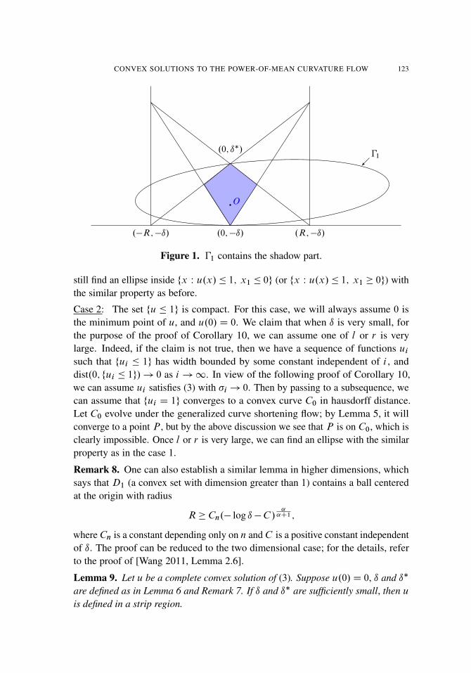
CONVEX SOLUTIONS TO THE POWER-OF-MEAN CURVATURE FLOW 123
.�R;�ı/ .0;�ı/ .R;�ı/
.0; ı�/
O
�1
Figure 1. �1 contains the shadow part.
still find an ellipse inside fx W u.x/� 1; x1 � 0g (or fx W u.x/� 1; x1 � 0g) withthe similar property as before.
Case 2: The set fu � 1g is compact. For this case, we will always assume 0 isthe minimum point of u, and u.0/D 0. We claim that when ı is very small, forthe purpose of the proof of Corollary 10, we can assume one of l or r is verylarge. Indeed, if the claim is not true, then we have a sequence of functions ui
such that fui � 1g has width bounded by some constant independent of i , anddist.0; fui � 1g/! 0 as i !1. In view of the following proof of Corollary 10,we can assume ui satisfies (3) with �i ! 0. Then by passing to a subsequence, wecan assume that fui D 1g converges to a convex curve C0 in hausdorff distance.Let C0 evolve under the generalized curve shortening flow; by Lemma 5, it willconverge to a point P , but by the above discussion we see that P is on C0, which isclearly impossible. Once l or r is very large, we can find an ellipse with the similarproperty as in the case 1.
Remark 8. One can also establish a similar lemma in higher dimensions, whichsays that D1 (a convex set with dimension greater than 1) contains a ball centeredat the origin with radius
R� Cn.� log ı�C /˛˛C1 ;
where Cn is a constant depending only on n and C is a positive constant independentof ı. The proof can be reduced to the two dimensional case; for the details, referto the proof of [Wang 2011, Lemma 2.6].
Lemma 9. Let u be a complete convex solution of (3). Suppose u.0/D 0, ı and ı�
are defined as in Lemma 6 and Remark 7. If ı and ı� are sufficiently small, then u
is defined in a strip region.

124 SHIBING CHEN
When ˛ D 1, this lemma is proved by Wang [2011, Corollary 2.2]. The proofof Lemma 9 is based on a careful study of the shape of the level set of u. Beforegiving the proof, we will give an important corollary first.
Corollary 10. Let u be an entire convex solution of (3) in R2, then
(18) u.x/� C.1Cjxj1C˛/;
where the constant C depends only on the upper bound for u.0/ and jDu.0/j.
Proof. The proof of this Corollary follows the proof of [Wang 2011, Theorem 2.1].We only record some necessary changes here. First, the rescaling uh.x/D
1hu.h
12 x/
used that proof should be replaced by uh.x/D1hu.h
11C˛ x/. Note that uh solves (3)
with � D �h! 0 as h!1. Second, the ellipse used in that proof when applyingthe comparison argument should be replaced by the one discussed in Remark 7. �
Proof of Lemma 9. By a rotation of coordinates we may assume that the axialdirections of E in Remark 7 coincide with those of the coordinate system. Let Mu
be the graph of u, which consists of two parts, Mu DMC[M�, where
MC D f.x;u.x// 2 R3W @x2
u� 0g and M� D f.x;u.x// 2 R3W @x2
u� 0g:
Then M˙ can be represented as the graphs of functions g˙ of the form x2 D
g˙.x1;x3/, for .x1;x3/ 2 D where D is the projection of Mu onto the planefx2 D 0g. The functions gC and g� are concave and convex, respectively, and wehave x3 D u.x1;g
˙.x1;x3//. Set
(19) g D gC�g�:
Then g is a positive, concave function on D, vanishing on @D. For any h> 0 letgh.x1/D g.x1; h/, g˙
h.x1/D g˙.x1; h/, and DhDfx1 2R1 W .x1; h/2Dg. Then
gh is a positive, concave function in Dh, vanishing on @Dh, and DhD .�ah; ah/ isan interval containing the origin. Let bh D gh.0/. We consider the case � D 0 first.
Claim 1: Suppose h is large, g1.0/ D ı�C ı is small, bh � 4, and ah; ah � bh.
Then,
ah �1
1000
h
b˛h
for ˛ � 1 and ah �1
1000
h1=.2˛�1/
b1=.2˛�1/
h
for ˛ > 1:
Proof. Without loss of generality, we assume ah � ah. Let Uh D�h \ fx1 > 0g.By the convexity of Uh and the assumption ah; ah � bh, we have as; as �
12bh for
all s 2�
12h; h
�. Hence by the concavity of g,ˇ
d
dx1gs.0/
ˇ� 2 for s 2
�12h; h
�;
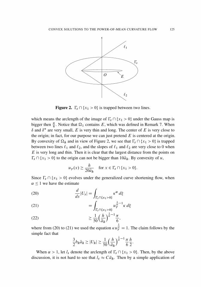
CONVEX SOLUTIONS TO THE POWER-OF-MEAN CURVATURE FLOW 125
`1
`2
�s
EO
Figure 2. �s \fx1 > 0g is trapped between two lines.
which means the arclength of the image of �s \fx1 > 0g under the Gauss map isbigger then �
6. Notice that �1 contains E, which was defined in Remark 7. When
ı and ı� are very small, E is very thin and long. The center of E is very close tothe origin; in fact, for our purpose we can just pretend E is centered at the origin.By convexity of �h and in view of Figure 2, we see that �s \fx1 > 0g is trappedbetween two lines `1 and `2, and the slopes of `1 and `2 are very close to 0 whenE is very long and thin. Then it is clear that the largest distance from the points on�s \fx1 > 0g to the origin can not be bigger than 10ah. By convexity of u,
u .x/�h
20ahfor x 2 �s \fx1 > 0g:
Since �s \ fx1 > 0g evolves under the generalized curve shortening flow, when˛ � 1 we have the estimate
d
dsjUsj D
Z�s\fx1>0g
�˛ d�(20)
D
Z�s\fx1>0g
u1˛�1
� d�(21)
�1
50
�h
ah
�1˛�1�
6;(22)
where from (20) to (21) we used the equation �u1˛ D 1. The claim follows by the
simple fact that3
2bhah � jUhj �
1
50
�h
ah
�1˛�1�
6
h
2:
When ˛ > 1, let ls denote the arclength of �s \ fx1 > 0g. Then, by the abovediscussion, it is not hard to see that ls � C ah. Then by a simple application of
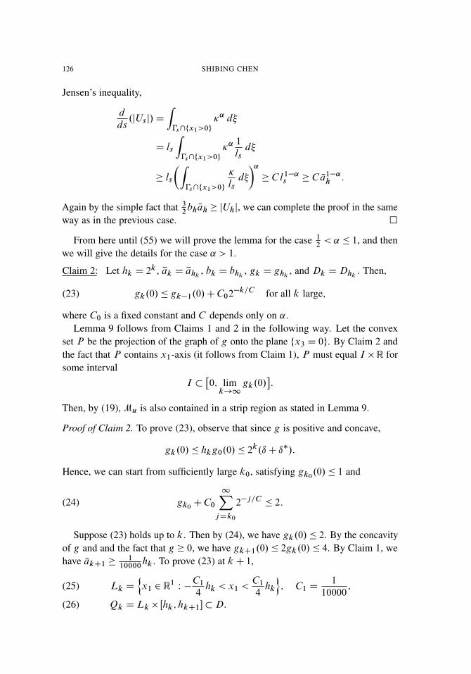
126 SHIBING CHEN
Jensen’s inequality,
d
ds.jUsj/D
Z�s\fx1>0g
�˛ d�
D ls
Z�s\fx1>0g
�˛1
lsd�
� ls
�Z�s\fx1>0g
�
lsd�
�� C l1�˛
s � C a1�˛h :
Again by the simple fact that 32bhah � jUhj, we can complete the proof in the same
way as in the previous case. �
From here until (55) we will prove the lemma for the case 12< ˛ � 1, and then
we will give the details for the case ˛ > 1.
Claim 2: Let hk D 2k , ak D ahk, bk D bhk
, gk D ghk, and Dk DDhk
. Then,
(23) gk.0/� gk�1.0/CC02�k=C for all k large;
where C0 is a fixed constant and C depends only on ˛.Lemma 9 follows from Claims 1 and 2 in the following way. Let the convex
set P be the projection of the graph of g onto the plane fx3 D 0g. By Claim 2 andthe fact that P contains x1-axis (it follows from Claim 1), P must equal I �R forsome interval
I ��0; lim
k!1gk.0/
�:
Then, by (19), Mu is also contained in a strip region as stated in Lemma 9.
Proof of Claim 2. To prove (23), observe that since g is positive and concave,
gk.0/� hkg0.0/� 2k.ıC ı�/:
Hence, we can start from sufficiently large k0, satisfying gk0.0/� 1 and
(24) gk0CC0
1XjDk0
2�j=C� 2:
Suppose (23) holds up to k. Then by (24), we have gk.0/� 2. By the concavityof g and and the fact that g � 0, we have gkC1.0/� 2gk.0/� 4. By Claim 1, wehave akC1 �
110000
hk . To prove (23) at kC 1,
Lk D
nx1 2 R1
W �C1
4hk < x1 <
C1
4hk
o; C1 D
1
10000;(25)
Qk DLk � Œhk ; hkC1��D:(26)
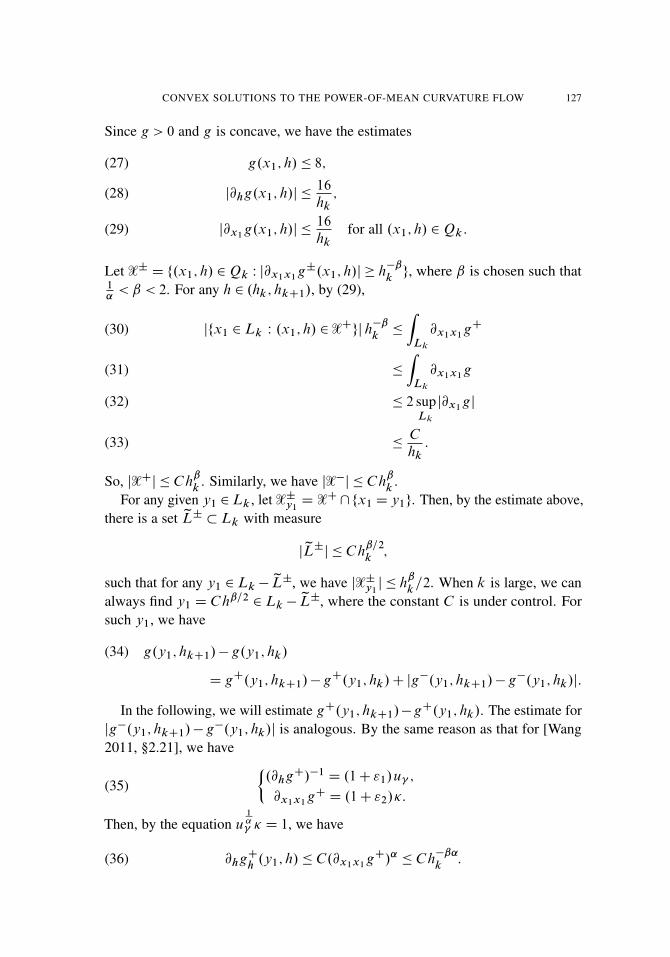
CONVEX SOLUTIONS TO THE POWER-OF-MEAN CURVATURE FLOW 127
Since g > 0 and g is concave, we have the estimates
g.x1; h/� 8;(27)
[email protected]; h/j �16
hk;(28)
[email protected]; h/j �
16
hkfor all .x1; h/ 2Qk :(29)
Let X˙ D f.x1; h/ 2Qk W j@x1x1g˙.x1; h/j � h
�ˇ
kg, where ˇ is chosen such that
1˛< ˇ < 2. For any h 2 .hk ; hkC1/, by (29),
jfx1 2Lk W .x1; h/ 2 XCgj h�ˇ
k�
ZLk
@x1x1gC(30)
�
ZLk
@x1x1g(31)
� 2 supLk
j@x1gj(32)
�C
hk:(33)
So, jXCj � C hˇ
k. Similarly, we have jX�j � C h
ˇ
k.
For any given y1 2Lk , let X˙y1D XC\fx1D y1g. Then, by the estimate above,
there is a set zL˙ �Lk with measure
j zL˙j � C hˇ=2
k;
such that for any y1 2Lk �zL˙, we have jX˙y1
j � hˇ
k=2. When k is large, we can
always find y1 D C hˇ=2 2Lk �zL˙, where the constant C is under control. For
such y1, we have
(34) g.y1; hkC1/�g.y1; hk/
D gC.y1; hkC1/�gC.y1; hk/Cjg�.y1; hkC1/�g�.y1; hk/j:
In the following, we will estimate gC.y1; hkC1/�gC.y1; hk/. The estimate forjg�.y1; hkC1/�g�.y1; hk/j is analogous. By the same reason as that for [Wang2011, §2.21], we have
(35)�.@hgC/�1 D .1C "1/u ;
@x1x1gC D .1C "2/�:
Then, by the equation u1˛ � D 1, we have
(36) @hgCh.y1; h/� C.@x1x1
gC/˛ � C h�ˇ˛
k:
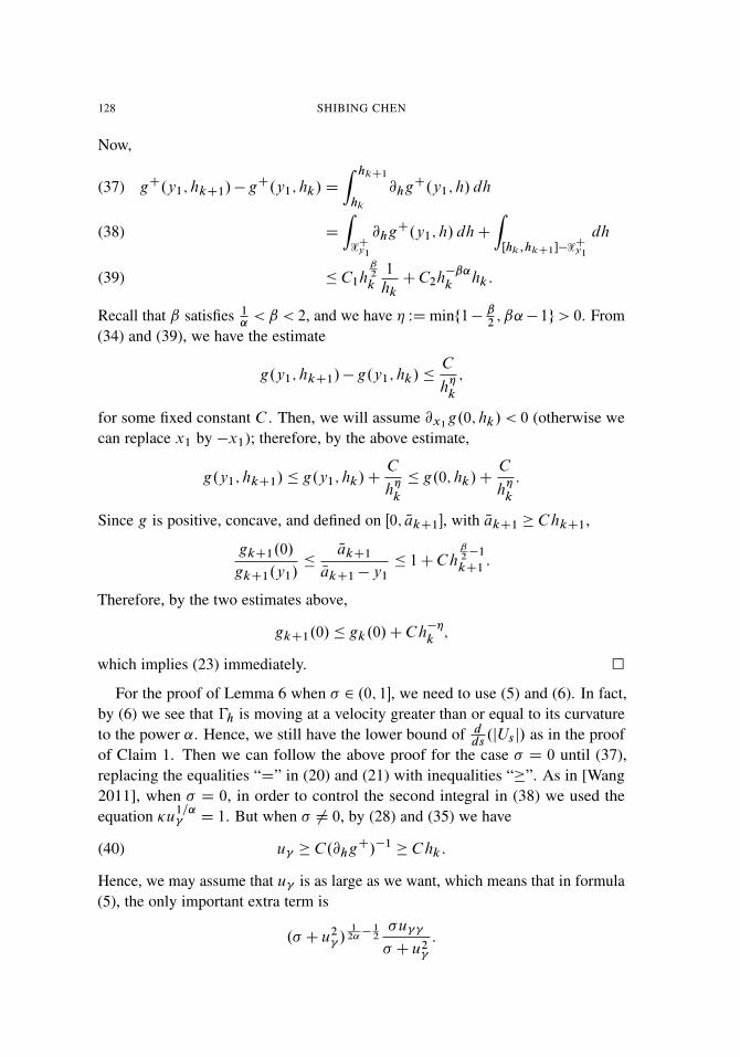
128 SHIBING CHEN
Now,
gC.y1; hkC1/�gC.y1; hk/D
Z hkC1
hk
@hgC.y1; h/ dh(37)
D
ZXCy1
@hgC.y1; h/ dhC
ZŒhk ;hkC1��XCy1
dh(38)
� C1hˇ2
k
1
hkCC2h
�ˇ˛
khk :(39)
Recall that ˇ satisfies 1˛< ˇ < 2, and we have � WDminf1� ˇ
2; ˇ˛�1g> 0. From
(34) and (39), we have the estimate
g.y1; hkC1/�g.y1; hk/�C
h�
k
;
for some fixed constant C . Then, we will assume @x1g.0; hk/ < 0 (otherwise we
can replace x1 by �x1); therefore, by the above estimate,
g.y1; hkC1/� g.y1; hk/CC
h�
k
� g.0; hk/CC
h�
k
:
Since g is positive, concave, and defined on Œ0; NakC1�, with NakC1 � C hkC1,
gkC1.0/
gkC1.y1/�
NakC1
NakC1�y1
� 1CC hˇ2�1
kC1:
Therefore, by the two estimates above,
gkC1.0/� gk.0/CC h��
k;
which implies (23) immediately. �
For the proof of Lemma 6 when � 2 .0; 1�, we need to use (5) and (6). In fact,by (6) we see that �h is moving at a velocity greater than or equal to its curvatureto the power ˛. Hence, we still have the lower bound of d
ds.jUsj/ as in the proof
of Claim 1. Then we can follow the above proof for the case � D 0 until (37),replacing the equalities “D” in (20) and (21) with inequalities “�”. As in [Wang2011], when � D 0, in order to control the second integral in (38) we used theequation �u
1=˛ D 1. But when � ¤ 0, by (28) and (35) we have
(40) u � C.@hgC/�1� C hk :
Hence, we may assume that u is as large as we want, which means that in formula(5), the only important extra term is
.� Cu2 /
12˛� 1
2�u
� Cu2
:
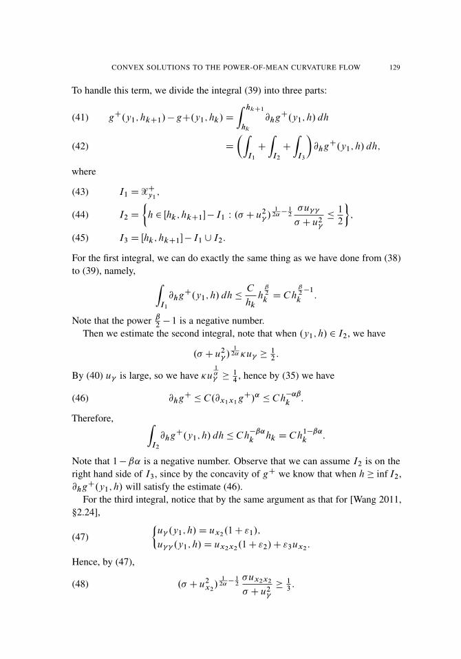
CONVEX SOLUTIONS TO THE POWER-OF-MEAN CURVATURE FLOW 129
To handle this term, we divide the integral (39) into three parts:
gC.y1; hkC1/�gC.y1; hk/D
Z hkC1
hk
@hgC.y1; h/ dh(41)
D
�ZI1
C
ZI2
C
ZI3
�@hgC.y1; h/ dh;(42)
where
I1 D XCy1;(43)
I2 D
�h 2 Œhk ; hkC1�� I1 W .� Cu2
/1
2˛� 1
2�u
� Cu2
�1
2
�;(44)
I3 D Œhk ; hkC1�� I1[ I2:(45)
For the first integral, we can do exactly the same thing as we have done from (38)to (39), namely, Z
I1
@hgC.y1; h/ dh�C
hk
hˇ2
kD C h
ˇ2�1
k:
Note that the power ˇ2� 1 is a negative number.
Then we estimate the second integral, note that when .y1; h/ 2 I2, we have
.� Cu2 /
12˛ �u �
12:
By (40) u is large, so we have �u1˛ �
14
, hence by (35) we have
(46) @hgC � C.@x1x1gC/˛ � C h
�˛ˇ
k:
Therefore, ZI2
@hgC.y1; h/ dh� C h�ˇ˛
khk D C h
1�ˇ˛
k:
Note that 1�ˇ˛ is a negative number. Observe that we can assume I2 is on theright hand side of I3, since by the concavity of gC we know that when h� inf I2,@hgC.y1; h/ will satisfy the estimate (46).
For the third integral, notice that by the same argument as that for [Wang 2011,§2.24],
(47)�
u .y1; h/D ux2.1C "1/;
u .y1; h/D ux2x2.1C "2/C "3ux2
:
Hence, by (47),
(48) .� Cu2x2/
12˛� 1
2�ux2x2
� Cu2
�13:
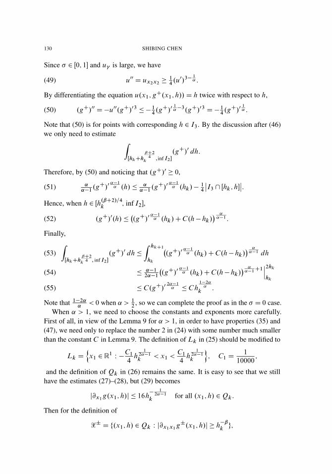
130 SHIBING CHEN
Since � 2 Œ0; 1� and u is large, we have
(49) u00 D ux2x2�
14.u0/3�
1˛ :
By differentiating the equation u.x1;gC.x1; h//D h twice with respect to h,
(50) .gC/00 D�u00.gC/03 � �14.gC/0
1˛�3.gC/03 D�1
4.gC/0
1˛ :
Note that (50) is for points with corresponding h 2 I3. By the discussion after (46)we only need to estimate Z
ŒhkChˇC2
4k
;inf I2�
.gC/0 dh:
Therefore, by (50) and noticing that .gC/0 � 0,
(51) ˛˛�1
.gC/0˛�1˛ .h/� ˛
˛�1.gC/0
˛�1˛ .hk/�
14
ˇI3\ Œhk ; h�
ˇ:
Hence, when h 2 Œh.ˇC2/=4
k; inf I2�,
(52) .gC/0.h/��.gC/0
˛�1˛ .hk/CC.h� hk/
� ˛˛�1 :
Finally,ZŒhkCh
ˇC24
k; inf I2�
.gC/0 dh�
Z hkC1
hk
�.gC/0
˛�1˛ .hk/CC.h� hk/
� ˛˛�1 dh(53)
�˛�1
2˛�1
�.gC/0
˛�1˛ .hk/CC.h� hk/
� ˛˛�1C1ˇ2hk
hk
(54)
� C.gC/02˛�1˛ � C h
1�2˛˛
k:(55)
Note that 1�2˛˛
< 0 when ˛ > 12
, so we can complete the proof as in the � D 0 case.When ˛ > 1, we need to choose the constants and exponents more carefully.
First of all, in view of the Lemma 9 for ˛ > 1, in order to have properties (35) and(47), we need only to replace the number 2 in (24) with some number much smallerthan the constant C in Lemma 9. The definition of Lk in (25) should be modified to
Lk D
nx1 2 R1
W �C1
4h
12˛�1
k< x1 <
C1
4h
12˛�1
k
o; C1 D
1
10000;
and the definition of Qk in (26) remains the same. It is easy to see that we stillhave the estimates (27)–(28), but (29) becomes
[email protected]; h/j � 16h
� 12˛�1
kfor all .x1; h/ 2Qk :
Then for the definition of
X˙ D f.x1; h/ 2Qk W j@x1x1g˙.x1; h/j � h
�ˇ
kg;

CONVEX SOLUTIONS TO THE POWER-OF-MEAN CURVATURE FLOW 131
we need to choose the exponent ˇ so that 1˛< ˇ < 2
2˛�1. By doing the same
computation as (30)–(32),ˇfx1 2Lk W .x1; h/ 2 XCg
ˇh�ˇ
k�
ZLk
@x1x1gC � C h
� 12˛�1
k:
Hence,
jXCj � C h1Cˇ� 1
2˛�1
kand jX�j � C h
1Cˇ� 12˛�1
k:
Then, by the above estimate there is a set zL˙ �Lk with measure
j zL˙j � C hˇC"� 1
2˛�1
k
such that for any y1 2 Lk �zL˙, we have jX˙y1
j � h1�"k
, where " is chosen suchthat ˇC " < 2
2˛�1. Now, (35)–(38) remain the same, and (39) becomes
gC.y1; hkC1/�gC.y1; hk/� C1h1�"k
1
hkCC2h
�ˇ˛
khk :
By the choice of ˇ, all the exponents of hk are negative. We do not need to changeanything from (40) to (49). Finally from (50) we need to replace the computationin the case ˛ � 1 with the following computation.
First, we have .gC/00 � �14.gC/0
1˛ � �
14.gC/0, and we only need to boundZ
ŒhkCh1�"=2
k; inf I2�
.gC/0 dh:
Note that .gC/0 � 0. By integrating the above differential inequality, we have
.gC/0.h/� .gC/0.hk/e� 1
4jI3j � .gC/0.hk/e
18.h�hk/
when h 2 Œhk C h1�"=2
k; inf I2�. Therefore, we haveZ
ŒhkCh1�"=2
k; inf I2�
.gC/0 dh�
Z hkC1
hk
.gC/0.hk/e18.h�hk/ dh
� C.gC/0.hk/�C
hk: �
3. Blow-down of an entire convex ancient solutionsconverges to a power function
In this section we prove that the blow-down of an entire convex solution to (3)converges to a power function.
Proof of Theorem 1 and the first part of Theorem 2. First, we prove that there is asubsequence of uh converging to 1
1C˛jxj1C˛, where uh.x/D h�1u.h
11C˛ x/.

132 SHIBING CHEN
By adding a constant we may suppose u.0/D 0. Let xnC1D a �x be the equationof the tangent plane of u at 0. By Corollary 10 and the convexity of u we have
a �x � u.x/� C.1Cjxj1C˛/:
Hence,h�
˛1C˛ a �x � uh.x/� C
�1hCjxj1C˛
�:
By convexity, Duh is locally uniformly bounded. Hence, uh subconverges to aconvex function u0 which satisfies u0.0/D 0, and
0� u0.x/� C jxj1C˛:
It is easy to check that u0 is an entire convex viscosity solution to (3) with � D 0,and the comparison principle holds on any bounded domain.
Now we will prove that fu0.x/ D 0g D f0g. In fact, if fx W u0.x/ D 0g is abounded set, then fu0.x/D hg is a closed, bounded convex curve which evolvesunder the generalized curve shortening flow; from [Andrews 1998] it follows thatfu0.x/D0gDf0g. If fu0.x/D0g contains a straight line, say the line f.t; 0/ W t 2Rg,then by convexity, u is independent of x1, which is impossible. So we only need torule out the possibility that fu0.x/D 0g contains a ray but no straight lines. In thiscase, for fixed h> 0, we can find an ellipse E inside fu0.x/ < hg, with the shortaxis bounded from below by a constant depending only on h and with the long axisas long as we want (one only needs to look at the asymptotic cone of fu0.x/D hg),but since fu0.x/ D hg evolves under the generalized curve shortening flow andE � fu0.x/� hg, this is impossible by comparison principle.
Then since fu0.x/D 0g D f0g, �1;u0D fu0.x/D 1g is a bounded convex curve,
and the level set fu0.x/ D �tg evolves under the generalized curve shorteningflow, with time t 2 .�1; 0/. From [Andrews 1998; 2003] we have the followingasymptotic behavior of the convex solution u0 of L0uD 1:
(56) u0.x/D1
1C˛jxj1C˛C'.x/;
where '.x/D o.jxj˛C1/ for x¤ 0 near the origin. In fact, if the initial level curve isin a sufficiently small neighborhood of circle, by Lemma 13, j'.x/j � C jxj1C˛C�
for some small positive �, where C is a constant depending only on the initialcloseness to the circle. Hence, given any � > 0, for sufficiently small h0 > 0,
B.1��/r .0/��h0;u0� B.1C�/r .0/;
where r D ..1C˛/h0/1
1C˛ . Hence, there is a sequence hm!1 such that
B.1� 1m/rm;i
.0/��hm;u � B.1C 1m/rm;i
.0/;
whererm;i D ..1C˛/ihm/
11C˛ ; i D 1; : : : ;m:

CONVEX SOLUTIONS TO THE POWER-OF-MEAN CURVATURE FLOW 133
Then uhmsubconverges to 1
1C˛jxj1C˛.
Since u0 is an entire convex solution to L0uD 1 (we still use the notation u0,but it means an arbitrary entire convex solution), from the above argument, we canfind a sequence hm such that
u0hm.x/D
1
hmu0
�h
11C˛m x
�locally uniformly converges to 1
1C˛jxj1C˛. Hence, the sublevel set � 1
1C˛;u0hm
satisfiesB1��m
.0/�� 11C˛
;u0hm� B1C�m
.0/;
where �m! 0 as m!1. By the discussion below (56),
u0hm.x/D 1
1C˛jxj1C˛C'.x/;
where j'.x/j � C jxj1C˛C� for some fixed small positive �, and the constant C isindependent of m. Replacing x by h
�1=.1C˛/m x in the asymptotic formula above,
u0.x/D1
1C˛jxj1C˛C hm'
�h� 1
1C˛m x
�;
where for any fixed x, hm'.h� 1
1C˛m x/! 0. Hence u0.x/ D
11C˛jxj1C˛. So we
have proved Theorem 1 and the first part of Theorem 2. �
4. One-dimensional entire convex ancient solutionmust be a shrinking circle
This section is devoted to the proof of Corollary 3, which is completed by combiningthe following lemma (corresponding to [Wang 2011, Lemma 4.1]) and Theorem 2.
Lemma 11. Let � be a smooth, bounded, convex domain in R2. Let u be thesolution of (3) with � D 0, vanishing on @�. Then for any constant h satisfyinginf� u < h < 0, the level set �h;u D fu D hg is convex. Moreover, log.�u/ is aconcave function.
Proof. Observe that ' WD � log.�u/ satisfies
jD'j1˛�1
2Xi;jD1
�ıij �
'i'j
jD'j2
�'ij D e
1˛':
Since '.x/!C1 as x! @�, [Kawohl 1985, Theorem 3.13] implies that ' isconvex. �
With the previous lemma and [Wang 2011, Lemma 4.4], we know that anyconvex compact ancient solution to the generalized curve shortening flow can berepresented as a convex solution u to (3) with � D 0, and if the solution to the flow
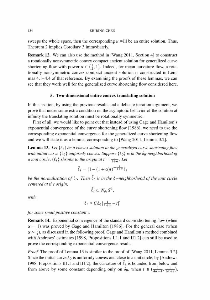
134 SHIBING CHEN
sweeps the whole space, then the corresponding u will be an entire solution. Thus,Theorem 2 implies Corollary 3 immediately.
Remark 12. We can also use the method in [Wang 2011, Section 4] to constructa rotationally nonsymmetric convex compact ancient solution for generalized curveshortening flow with power ˛ 2
�12; 1�. Indeed, for mean curvature flow, a rota-
tionally nonsymmetric convex compact ancient solution is constructed in Lem-mas 4.1–4.4 of that reference. By examining the proofs of these lemmas, we cansee that they work well for the generalized curve shortening flow considered here.
5. Two-dimensional entire convex translating solution
In this section, by using the previous results and a delicate iteration argument, weprove that under some extra condition on the asymptotic behavior of the solution atinfinity the translating solution must be rotationally symmetric.
First of all, we would like to point out that instead of using Gage and Hamilton’sexponential convergence of the curve shortening flow [1986], we need to use thecorresponding exponential convergence for the generalized curve shortening flowand we will state it as a lemma, corresponding to [Wang 2011, Lemma 3.2].
Lemma 13. Let f`tg be a convex solution to the generalized curve shortening flowwith initial curve f`0g uniformly convex. Suppose f`0g is in the ı0-neighborhood ofa unit circle, f`tg shrinks to the origin at t D 1
1C˛. Let
Qt D .1� .1C˛/t/
� 11C˛ `t
be the normalization of `t . Then Qt is in the ıt -neighborhood of the unit circlecentered at the origin,
Qt �Nıt
S1;
withıt � Cı0
�1
1C˛� t��
for some small positive constant �.
Remark 14. Exponential convergence of the standard curve shortening flow (when˛ D 1) was proved by Gage and Hamilton [1986]. For the general case (when˛ > 1
3), as discussed in the following proof, Gage and Hamilton’s method combined
with Andrews’ estimates [1998, Propositions II1.1 and II1.2] can still be used toprove the corresponding exponential convergence result.
Proof. The proof of Lemma 13 is similar to the proof of [Wang 2011, Lemma 3.2].Since the initial curve `0 is uniformly convex and close to a unit circle, by [Andrews1998, Propositions II1.1 and II1.2], the curvature of Qt is bounded from below andfrom above by some constant depending only on ı0, when t 2
�1
4˛C4; 1
2˛C2
�.

CONVEX SOLUTIONS TO THE POWER-OF-MEAN CURVATURE FLOW 135
Hence the evolution equation for Qt is uniformly parabolic. Therefore, we can applySchauder’s estimates safely for ˛ > 1
2, as in [Wang 2011], which says that
k Qt �S1k
C k � Cı0 for t 2�
14˛C4
; 12˛C2
�:
Although the constant C will depend on the lower and upper bounds of the curvatureof the initial curve, it is not a problem for our purpose, since when we blow downthe solution for � D 0, the norm of the gradient Duh on the curve fuh.x/ D 1g
approaches 1.By the equation �u
1˛ D 1, we see that the curvature � is also very close to 1
on that curve. For the exponential decay rate of the derivative of curvature, onecan imitate the proof in [Gage and Hamilton 1986, §§5.7.10–5.7.15], and ourcorresponding estimate will be j�0.�/j �Cı0e��� for some small positive number �,where � D� 1
1C˛log�
11C˛� t�. Indeed, in the case ˛ > 1, this is done by Chen and
Huang [Huang 2011, Corollary 3.2], and it is easy to check that their computationalso works for the case 1
3< ˛ < 1 by taking ` small enough. This estimate
immediately implies our lemma. �
In the following we will consider the case when � D 1 and ˛ > 1. By translatingand adding some constant we can assume u.0/D inf u. Let
uh.x/D1
hu.h
11C˛ x/:
Then uh satisfies the equation L�uh D 1 with � D h�2˛
1C˛ . By Theorem 1, uh
converges to 11C˛jxj1C˛, and the level set � 1
1C˛;uh
converges to the unit circle ash!1.
Lemma 15 [Wang 2011, Lemma 3.3]. The function u satisfies
(57) u.x/D 11C˛jxj1C˛CO.jxj1C˛�2˛ˇ/;
where ˇ is a constant, chosen such that 12˛< ˇ <min
˚1; 1C˛
2˛
.
Proof. For any given small ı0 > 0, take h sufficiently large such that
(58) � 11C˛
;uh�Nı0
.S1/
for the unit circle S1 with center p0. Note that when h is large, ı0 is very closeto 0. Then we will prove the following claim:
Claim 3: For small fixed � ,
(59) ��;uh� ..1C˛/�/
11C˛ Nı�
�.1C a0
�/
11C˛S1
�with
(60) ı� � C1.�/�ˇCC2ı0�
�;

136 SHIBING CHEN
where � is a small positive constant, the constants C1 and C2 are independent of ı0and h, and C2 is also independent of � . Let u0 be the solution of
L0.u/D 1 in � 11C˛
;uh;
satisfyingu0 D uh D
11C˛
on @� 11C˛
;uh;
where a0 D jinf u0j and the center of
.1C a0
�/
11C˛S1
is the minimum point of u0 multiplied by the factor ..1C˛/�/�1
1C˛ .
Proof of Claim 3. We only need to prove that
(61) dist�.1C˛/
11C˛ .� C a0/
11C˛S1; ��;u
�� C1.�/�
ˇCC2ı0�
11C˛C�;
where � is some small positive constant and C2 is independent of � . By Theorem 1we know that uh converges to 1
1C˛jxj1C˛ uniformly on any compact subset of R2:
Then by the convexity of uh, we have that jDuhj is bounded above and below bysome constants depending on �0 for large h when
x 2˚x 2� 1
1C˛;uhW �0 � uh <
11C˛
:
Hence, by the growth condition for D2u in Theorem 2, we have �.uh/ � C�ˇ;
where C is a constant depending on �0. Therefore, we have
�.uh/1=˛ � 1�C�ˇ on
˚x 2� 1
1C˛;uhW � � uh <
11C˛
;
where C depends on �0. Let
Qu0 D .1�C�ˇ/˛.u0�1
1C˛/C 1
1C˛I
thenL0. Qu0/D 1�C�ˇ in � 1
1C˛;uh
withQu0 D uh D
11C˛
on @� 11C˛
;uh:
Now by the comparison principle, ��;u0���;uh
���; Qu0, and by the asymptotic
behavior of u0,
��;u0�N�
�.� C a0/
11C˛S1
�and ��;Qu0
�N��.� C a0�C�ˇ/
11C˛S1
�;
where � D Cı0.� C a0/�. Let
`1 D .� C a0/1
1C˛S1 and `2 D .� C a0�C�ˇ/1
1C˛S1;
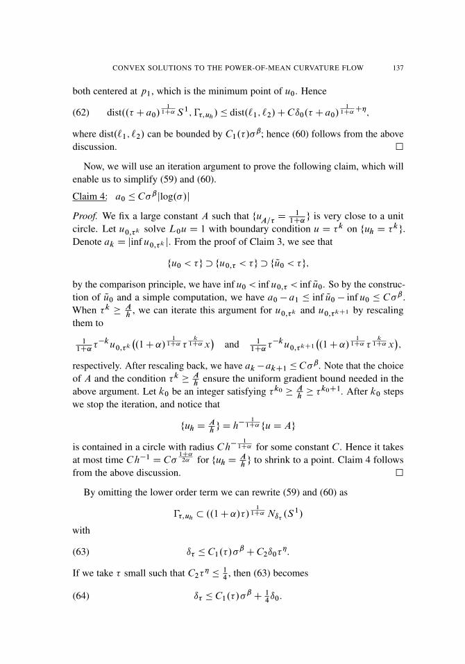
CONVEX SOLUTIONS TO THE POWER-OF-MEAN CURVATURE FLOW 137
both centered at p1, which is the minimum point of u0. Hence
(62) dist..� C a0/1
1C˛S1; ��;uh/� dist.`1; `2/CCı0.� C a0/
11C˛C�;
where dist.`1; `2/ can be bounded by C1.�/�ˇ; hence (60) follows from the above
discussion. �
Now, we will use an iteration argument to prove the following claim, which willenable us to simplify (59) and (60).
Claim 4: a0 � C�ˇjlog.�/j
Proof. We fix a large constant A such that fuA=�D
11C˛g is very close to a unit
circle. Let u0;�k solve L0u D 1 with boundary condition u D �k on fuh D �kg.
Denote ak D jinf u0;�k j. From the proof of Claim 3, we see that
fu0 < �g � fu0;� < �g � f Qu0 < �g;
by the comparison principle, we have inf u0 < inf u0;� < inf Qu0. So by the construc-tion of Qu0 and a simple computation, we have a0 � a1 � inf Qu0 � inf u0 � C�ˇ.When �k �
Ah
, we can iterate this argument for u0;�k and u0;�kC1 by rescalingthem to
11C˛
��ku0;�k
�.1C˛/
11C˛ �
k1C˛ x
�and 1
1C˛��ku0;�kC1
�.1C˛/
11C˛ �
k1C˛ x
�;
respectively. After rescaling back, we have ak �akC1 �C�ˇ. Note that the choiceof A and the condition �k �
Ah
ensure the uniform gradient bound needed in theabove argument. Let k0 be an integer satisfying �k0 �
Ah� �k0C1. After k0 steps
we stop the iteration, and notice that
fuh DAhg D h�
11C˛ fuDAg
is contained in a circle with radius C h�1
1C˛ for some constant C . Hence it takesat most time C h�1 D C�
1C˛2˛ for fuh D
Ahg to shrink to a point. Claim 4 follows
from the above discussion. �
By omitting the lower order term we can rewrite (59) and (60) as
��;uh� ..1C˛/�/
11C˛ Nı� .S
1/
with
(63) ı� � C1.�/�ˇCC2ı0�
�:
If we take � small such that C2�� �
14
, then (63) becomes
(64) ı� � C1.�/�ˇC
14ı0:
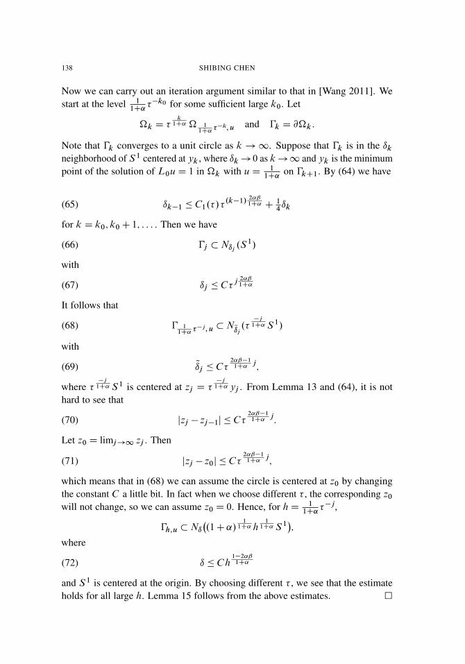
138 SHIBING CHEN
Now we can carry out an iteration argument similar to that in [Wang 2011]. Westart at the level 1
1C˛��k0 for some sufficient large k0. Let
�k D �k
1C˛ � 11C˛
��k;u and �k D @�k :
Note that �k converges to a unit circle as k !1. Suppose that �k is in the ıkneighborhood of S1 centered at yk , where ık!0 as k!1 and yk is the minimumpoint of the solution of L0uD 1 in �k with uD 1
1C˛on �kC1. By (64) we have
(65) ık�1 � C1.�/�.k�1/ 2˛ˇ
1C˛ C14ık
for k D k0; k0C 1; : : : . Then we have
(66) �j �Nıj .S1/
with
(67) ıj � C�j 2˛ˇ1C˛
It follows that
(68) � 11C˛
��j;u �NQıj.��j
1C˛S1/
with
(69) Qıj � C�2˛ˇ�1
1C˛j;
where ��j
1C˛S1 is centered at zj D ��j
1C˛ yj . From Lemma 13 and (64), it is nothard to see that
(70) jzj � zj�1j � C�2˛ˇ�1
1C˛j:
Let z0 D limj!1 zj . Then
(71) jzj � z0j � C�2˛ˇ�1
1C˛j;
which means that in (68) we can assume the circle is centered at z0 by changingthe constant C a little bit. In fact when we choose different � , the corresponding z0
will not change, so we can assume z0 D 0. Hence, for hD 11C˛
��j,
�h;u �Nı�.1C˛/
11C˛ h
11C˛S1
�;
where
(72) ı � C h1�2˛ˇ
1C˛
and S1 is centered at the origin. By choosing different � , we see that the estimateholds for all large h. Lemma 15 follows from the above estimates. �
CONVEX SOLUTIONS TO THE POWER-OF-MEAN CURVATURE FLOW 139
Remark 16. For the mean curvature flow (when ˛ D 1), I learned the proofof Claim 4 from Professor Xu-Jia Wang. Indeed, in this case one can do it asfollows. Let vk solve L0w D 1 with boundary condition w D �k on fuh D �
kg,for k D 1; 2; : : : . Let ak D jinf vk j. Then by [Wang 2011, Lemma 3.1], we havea0� a1 � C� . By rescaling invariance, we can iterate the argument to show thatak � akC1 � C� , provided �k �
1h
. Hence, we stop the iteration at k0 when�k0 �
1h> �k0C1. Notice that
fuh � �k0g D h�
12 fuD h�k0g � h�
12 fu� 1
�g:
So, it is easy to see that it takes at most time C� D Ch
for fuh � �k0g to shrink to a
point, namely, ak0� C� . Therefore,
a0 D ak0C
k0�1XiD0
ai � aiC1 � C k0� � C� jlog � j:
In order to finish the proof of Theorem 2 we need to use the following fundamentalLiouville theorem by Bernstein [Simon 1997, p. 245].
Lemma 17. Let u be an entire solution to the elliptic equationnX
i;jD1
aij .x/uij D 0 in R2:
If u satisfies the asymptotic estimate
ju.x/j D o.jxj/ as x!1;
then u is a constant.
Proof of the second part of Theorem 2. Let u� be the Legendre transform of u.Then u� satisfies equation
(73) G.x;D2u�/Ddet D2u��
ıij �xi xj
1Cjxj2
�F ij .u�/
D .1Cjxj2/1
2˛� 1
2 ;
where F ij .u�/D @ det r@rij
at r DD2u�. We have
(74) u�.x/D C.˛/jxj1C˛CO�jxj
1C˛�2˛ˇ˛
�;
where C.˛/ is a constant depending only on ˛. In fact, for big h, by Lemma 15,
uh.x/D1
1C˛jxj1C˛CO
�jhj�2˛ˇ1C˛
�in B1.0/. Denote by u�
hthe Legendre transform of uh. Then,
u�h .x/D C.˛/jxj1C1˛ CO
�jhj�2˛ˇ1C˛
�;

140 SHIBING CHEN
where C.˛/ is a constant depending only on ˛ and it comes from the Legendretransform of the function 1
1C˛jxj1C˛. Note that u�
h.x/ D h�1u�.h
˛1C˛ x/, we
obtain (74).Let u0 be the unique radial solution of (3) with � D 1, and let u�
0be the Legendre
transform of u0. Similar to (74) we have
(75) u�0 .x/D C.˛/jxj1C˛CO.jxj1C˛�2˛ˇ
˛ /:
Since both u� and u�0
satisfy (73), v D u��u�0
satisfies the elliptic equation
nXi;jD1
aij .x/vij D 0 in R2;
where
aij D
Z 1
0
Gij .x;D2u�0 C t.D2u��D2u�0 // dt:
Here,
@rij
for any symmetric matrix r . Note that by the choice of ˇ, 1C˛�2˛ˇ˛
< 1; hence, by(74) and (75),
v DO�jxj
1C˛�2˛ˇ˛
�D o.jxj/ as jxj !1:
By Lemma 17 we conclude that v is a constant. �
References
[Andrews 1998] B. Andrews, “Evolving convex curves”, Calc. Var. PDE 7:4 (1998), 315–371.MR 99k:58038 Zbl 0931.53030
[Andrews 2002] B. Andrews, “Non-convergence and instability in the asymptotic behaviour ofcurves evolving by curvature”, Comm. Anal. Geom. 10:2 (2002), 409–449. MR 2003e:53086Zbl 1029.53079
[Andrews 2003] B. Andrews, “Classification of limiting shapes for isotropic curve flows”, J. Amer.Math. Soc. 16:2 (2003), 443–459. MR 2004a:53083 Zbl 1023.53051
[Chou and Zhu 2001] K.-S. Chou and X.-P. Zhu, The curve shortening problem, Chapman &Hall/CRC, Boca Raton, FL, 2001. MR 2003e:53088 Zbl 1061.53045
[Daskalopoulos et al. 2010] P. Daskalopoulos, R. Hamilton, and N. Sesum, “Classification of com-pact ancient solutions to the curve shortening flow”, J. Differential Geom. 84:3 (2010), 455–464.MR 2012d:53213 Zbl 1205.53070
[Gage and Hamilton 1986] M. Gage and R. S. Hamilton, “The heat equation shrinking convex planecurves”, J. Differential Geom. 23:1 (1986), 69–96. MR 87m:53003 Zbl 0621.53001
[Huang 2011] R. L. Huang, “Blow-up rates for the general curve shortening flow”, J. Math. Anal.Appl. 383:2 (2011), 482–489. MR 2012h:53152 Zbl 1220.53082

CONVEX SOLUTIONS TO THE POWER-OF-MEAN CURVATURE FLOW 141
[Kawohl 1985] B. Kawohl, Rearrangements and convexity of level sets in PDE, Lecture Notes inMathematics 1150, Springer, Berlin, 1985. MR 87a:35001 Zbl 0593.35002
[Schulze 2005] F. Schulze, “Evolution of convex hypersurfaces by powers of the mean curvature”,Math. Z. 251:4 (2005), 721–733. MR 2006h:53065 Zbl 1087.53062
[Sheng and Wu 2009] W. Sheng and C. Wu, “On asymptotic behavior for singularities of the powers ofmean curvature flow”, Chin. Ann. Math. .B/ 30:1 (2009), 51–66. MR 2010h:53100 Zbl 1180.53066
[Simon 1997] L. Simon, “The minimal surface equation”, pp. 239–266 in Geometry V, edited by R.Osserman, Encyclopaedia of Mathematical Sciences 90, Springer, Berlin, 1997. MR 99b:53014Zbl 0905.53003
[Wang 2011] X.-J. Wang, “Convex solutions to the mean curvature flow”, Ann. of Math. .2/ 173:3(2011), 1185–1239. MR 2800714 Zbl 1231.53058
[White 2000] B. White, “The size of the singular set in mean curvature flow of mean-convex sets”, J.Amer. Math. Soc. 13:3 (2000), 665–695. MR 2001j:53098 Zbl 0961.53039
Received February 19, 2013. Revised October 19, 2014.
SHIBING CHEN
DEPARTMENT OF MATHEMATICS
ZHEJIANG UNIVERSITY OF TECHNOLOGY
HANGZHOU, ON 310023CHINA
Current address:MATHEMATICAL SCIENCES INSTITUTE
THE AUSTRALIAN NATIONAL UNIVERSITY
JOHN DEDMAN BUILDING 27CANBERRA ACT 2601AUSTRALIA

PACIFIC JOURNAL OF MATHEMATICSVol. 276, No. 1, 2015
dx.doi.org/10.2140/pjm.2015.276.143
CONSTRUCTIONS OF PERIODIC MINIMAL SURFACESAND MINIMAL ANNULI IN SOL3
CHRISTOPHE DESMONTS
We construct two one-parameter families of minimal properly embeddedsurfaces in the Lie group Sol3 using a Weierstrass-type representation.These surfaces are not invariant by a one-parameter group of ambientisometries. The first one can be viewed as a family of helicoids, and thesecond one as a family of minimal annuli called catenoids. Finally we studylimits of these catenoids, and in particular we show that one of these limitsis a new minimal entire graph.
1. Introduction
The aim of this paper is to construct two one-parameter families of examples ofproperly embedded minimal surfaces in the Lie group Sol3, endowed with itsstandard metric. This Lie group is a homogeneous Riemannian manifold with a3-dimensional isometry group and is one of the eight Thurston geometries. Thereis no rotation in Sol3, and so no surface of revolution.
The Hopf differential, which exists on surfaces in every 3-dimensional spaceform, has been generalized by Abresch and Rosenberg [2004; 2005] to every3-dimensional homogeneous Riemannian manifold with 4-dimensional isometrygroup. This tool leads to a lot of works in the field of constant mean curvature(CMC) surfaces in Nil3, APSL2.R/ and in the Berger spheres. More precisely,Abresch and Rosenberg [2005] proved that the generalized Hopf differential existsin a simply connected Riemannian 3-manifold if and only if its isometry group hasat least dimension 4.
Berdinskii and Taimanov [2005] gave a representation formula for minimalsurfaces in 3-dimensional Lie groups in terms of spinors, but they pointed outsome difficulties for using this theory in the case of Sol3. Nevertheless, someexplicit simple examples of minimal surfaces in Sol3 have been constructed inthe past decade. Masaltsev [2006] and Daniel and Mira [2013] gave some basicexamples of minimal graphs in Sol3: x1 D ax2C b, x1 D ae�x3 , x1 D ax2e�x3
and x1 D x2e�2x3 (and their images by ambient isometries). López and Munteanu
MSC2010: 53A10.Keywords: periodic minimal surfaces, minimal annuli, Sol3.
143

144 CHRISTOPHE DESMONTS
[2011; 2012; 2014], López [2014] and Masaltsev [2006] studied minimal surfacesin Sol3 invariant by a one-parameter group of ambient isometries. Finally, AnaMenezes [2014] constructed singly and doubly periodic Scherk minimal surfacesin Nil3 and Sol3, and Minh Hoang Nguyen [2014] gave conditions for the Dirichletproblem for the minimal surface equation in Sol3 to have solutions.
The method that we use in this paper is the one used by Daniel and Hauswirth[2009] in Nil3 to construct minimal embedded annuli: We first construct a one-parameter family of embedded minimal surfaces called helicoids and we calculateits Gauss map g. A result of Inoguchi and Lee [2008] shows that this map isharmonic for a certain metric on C. Then we seek another family of maps g withseparated variables that still satisfies the harmonic map equation, and we use aWeierstrass-type representation given by Inoguchi and Lee to construct a minimalimmersion whose Gauss map is g. We prove that these immersions are periodic,so we get minimal annuli. As far as the authors know, these annuli are the firstexamples of nonsimply connected minimal surfaces with finite topology (that is,diffeomorphic to a compact surface without a finite number of points) in Sol3.
The model we use for Sol3 is described in Section 2. In the third section, wegive some properties of the Gauss map of a conformal minimal immersion inSol3 (see [Daniel and Mira 2013]). In the fourth section, we construct the family.HK /K2��1I1Œ of helicoids, and finally we construct the family .C˛/˛2��1I1Œnf0g ofembedded minimal annuli. The study of the limit case of the parameter of thisfamily gives another example of a minimal surface in Sol3, which is an entire graph.None of these surfaces is invariant by a one-parameter family of isometries.
Theorem. There exists a one-parameter family .C˛/˛2��1I1Œnf0g of properly embed-ded minimal annuli in Sol3, called catenoids, having the following properties:
(1) The intersection of C˛ with any plane fx3D �g is a nonempty closed embeddedconvex curve.
(2) The annulus C˛ is conformally equivalent to C nf0g.
(3) The annulus C˛ has three symmetries fixing the origin: rotation by � aroundthe x3-axis, reflection in fx1 D 0g and reflection in fx2 D 0g.
2. The Lie group Sol3
Definition. The Lie group Sol3 is R3 with the multiplication � defined by
.x1;x2;x3/� .y1;y2;y3/D .y1e�x3 Cx1;y2ex3 Cx2;x3Cy3/
for all .x1;x2;x3/; .y1;y2;y3/ 2 R3. The identity element is 0 and the inverseelement of .x1;x2;x3/ is .x1;x2;x3/
�1 D .�x1ex3 ;�x2e�x3 ;�x3/. The Liegroup is noncommutative.
PERIODIC MINIMAL SURFACES AND MINIMAL ANNULI IN SOL3 145
The left multiplication la by an element aD .a1; a2; a3/ 2 R3 is given for allx D .x1;x2;x3/ 2 R3 by
la.x/D a�x D .x1e�a3 C a1;x2ea3 C a2; a3Cx3/
D aCMax;
where
Ma D
0@e�a3 0 0
0 ea3 0
0 0 1
1A :For the metric . �; � / on Sol3 to be left-invariant, it has to satisfy
.MaX;MaY /a�x D .X;Y /x
for all a;x;X;Y 2R3. We define a left-invariant Riemannian metric for x;X;Y 2R3
by the formula
(1) .X;Y /x D hMx�1X;Mx�1Y i;
where h � ; � i is the canonical scalar product on R3 and x�1 is the inverse elementof x in Sol3. The formula (1) leads to the expression of the previous metric
(2) ds2x D e2x3 dx2
1 C e�2x3 dx22 C dx2
3 ;
where .x1;x2;x3/ are canonical coordinates of R3. Since the translations areisometries now, Sol3 is a homogeneous manifold with this metric.
Remark. This metric is not the only possible left-invariant one on Sol3. In fact,there exists a two-parameter family of nonisometric left-invariant metrics on Sol3.One of these parameters is a homothetic one. The metrics that are nonhomotheticto (2) have no reflections; see [Meeks and Pérez 2012].
By setting
E1.x/D e�x3 @1; E2.x/D ex3 @2; and E3.x/D @3;
we obtain a left-invariant orthonormal frame .E1;E2;E3/. Thus, we now have twoframes to express the coordinates of a vector field on Sol3; we will use brackets todenote the coordinates in the frame .E1;E2;E3/; then at a point x 2 Sol3, we have
(3) a1 @1C a2 @2C a3 @3 D
0@a1
a2
a3
1AD24 ex3a1
e�x3a2
a3
35 :The following property holds (see [Daniel and Mira 2013]):

146 CHRISTOPHE DESMONTS
Proposition 1. The isotropy group of the origin of Sol3 is isomorphic to the dihe-dral group D4 and generated by orientation-reversing isometries
� W .x1;x2;x3/ 7�! .x2;�x1;�x3/ and � W .x1;x2;x3/ 7�! .�x1;x2;x3/;
whose orders are 4 and 2, respectively.
While � is simply a reflection in the plane fx1 D 0g, the generator � can bedescribed as a rotation by ��=3 around E3 composed with reflection in fx3 D 0g.The cyclic group h�i also contains �3 D ��1 and �2, the reflection in E3 (rotationby � around E3). The remaining nonidentity elements of the isotropy groupof the origin are �� and �3� , which are respectively the reflections in the linesf.x1;x1; 0/g and f.x1;�x1; 0/g, and �2� , which is reflection in the plane fx2D 0g.
We deduce the following theorem:
Theorem 2. The isometry group of Sol3 has dimension 3.
Finally, we express the Levi-Civita connection r of Sol3 associated to the metricgiven by (2) in the frame .E1;E2;E3/. First, we calculate the Lie brackets of thevectors of the frame. The Lie bracket in the Lie algebra sol3 of Sol3 is given by
ŒX;Y �D .Y3X1�X3Y1;X3Y2�Y3X2; 0/
for all X D .X1;X2;X3/ and Y D .Y1;Y2;Y3/. Then we have
ŒE1;E2�D 0; ŒE1;E3�DE1; ŒE2;E3�D�E2:
Hence,rE1
E1 D�E3; rE2E1 D 0; rE3
E1 D 0;
rE1E2 D 0; rE2
E2 DE3; rE3E2 D 0;
rE1E3 DE1; rE2
E3 D�E2; rE3E3 D 0:
3. The Gauss map
Let † be a Riemann surface and z D uC iv local complex coordinates in †. Letx W†! Sol3 be a conformal immersion. We set
x D
0@x1
x2
x3
1A ;and we define � 2 R�C by
2.xz;xNz/D kxuk2D kxvk
2D �:
PERIODIC MINIMAL SURFACES AND MINIMAL ANNULI IN SOL3 147
Thus, a unit normal vector field is N W†! T Sol3 defined by
N D�2i
�xz ^xNz WD
24N1
N2
N3
35 :Hence we define yN W†! S2 � R3 by the formula Mx�1N D yN , that is,
yN D
0@ex3 0 0
0 e�x3 0
0 0 1
1A0@N1e�x3
N2ex3
N3
1AD0@N1
N2
N3
1A :Definition. The Gauss map of the immersion x is the application
g D � ı yN W† �! C[f1g D C;
where � is the stereographic projection with respect to the southern pole, i.e.,
N D1
1Cjgj2
24 2<.g/
2=.g/
1� jgj2
35 ;(4)
g DN1C iN2
1CN3
:(5)
The following result is due to [Inoguchi and Lee 2008]. It can be viewed as aWeierstrass representation in Sol3.
Theorem 3. Let x W†! Sol3 be a conformal minimal immersion and g W†! C
its Gauss map. Then, whenever g is neither real nor purely imaginary, it is nowhereantiholomorphic (gz ¤ 0 for every point for any local conformal parameter z on†),and it satisfies the second order elliptic equation
(6) gz Nz D2ggzg
Nz
g2� Ng2:
Moreover, the immersion x D .x1;x2;x3/ can be expressed in terms of g by therepresentation formulas
(7) x1z D e�x3. Ng2� 1/gz
g2� Ng2; x2z D iex3
. Ng2C 1/gz
g2� Ng2; x3z D
2 Nggz
g2� Ng2
whenever it is well-defined.Conversely, given a map g W †! C defined on a simply connected Riemann
surface † satisfying (6), then the map x W †! Sol3 given by the representationformulas (7) is a conformal minimal immersion with possibly branched pointswhenever it is well-defined, and its Gauss map is g.

148 CHRISTOPHE DESMONTS
Remark. (1) There exists a similar result for the case of CMC H -surfaces ; see[Daniel and Mira 2013].
(2) Equation (6) is the harmonic map equation for maps g W†! .C; ds2/ equippedwith the metric
ds2Djd!j2
j!2� N!2j:
This is a singular metric, not defined on the real and pure imaginary axes. See[Inoguchi and Lee 2008] for more details.
(3) Equation (6) can be only considered at points where g ¤ 1. But if g is asolution of (6), i=g is also a solution at points where g ¤ 0. The conjugate map Ngand every g ı �, with � a locally injective holomorphic function, are solutionstoo. Moreover, if g is a nowhere antiholomorphic solution of (6), and x is theinduced conformal minimal immersion, then ig and 1=g induce conformal minimalimmersions given by �x and �x. Finally, Ng is the Gauss map of �2�x after achange of orientation.
Definition. The Hopf differential of the map g is the quadratic form
QD q dz2D
gz Ngz
g2� Ng2dz2:
Remark. (1) The function q depends on the choice of coordinates, whereas Q
does not.
(2) As stated in the introduction, the Hopf differential (or its Abresch–Rosenberggeneralization) is not defined on Sol3. If we apply the definition of the Hopfdifferential of the harmonic maps on .C; ds2/, we get
QDgz Ngz
jg2� Ng2jdz2;
but this leads to a nonsmooth differential. Because g2 � Ng2 is purely imaginaryon each quarter of the complex plane, the definitions are related by multiplicationby i or �i , depending on the quarter. Thus, this “Hopf differential” is defined andholomorphic only on each of the four quarters delimited by the real and purelyimaginary axes.
4. Construction of the helicoids in Sol3
In this section we construct a one-parameter family of helicoids in Sol3: we define ahelicoid to be a minimal surface containing the x3-axis whose intersection with everyplane fx3 D constantg is a straight line and which is invariant by left multiplicationby an element of Sol3 of the form .0; 0;T / for some T ¤ 0.

PERIODIC MINIMAL SURFACES AND MINIMAL ANNULI IN SOL3 149
Theorem 4. There exists a one-parameter family .HK /K2��1I1Œnf0g of properlyembedded minimal helicoids in Sol3 having the following properties:
(1) For all K 2 ��1I 1Œnf0g, the surface HK contains the x3-axis.
(2) For all K 2 ��1I 1Œnf0g, the intersection of HK and any horizontal planefx3 D �g is a straight line.
(3) For all K 2 ��1I 1Œnf0g, there exists TK such that HK is invariant by leftmultiplication by .0; 0;TK /.
(4) The helicoids HK have three symmetries fixing the origin: rotation by � aroundthe x3-axis, rotation by � around the .x;x; 0/-axis and rotation by � aroundthe .x;�x; 0/-axis.
Let K 2 ��1; 1Œ; we define a map g W C! C by
g.z D uC iv/D e�ueib.v/e�i�=4;
where b satisfies the ODE
(8) b0 Dp
1�K cos .2b/; b.0/D 0:
Proposition 5. The map b is well-defined and has the following properties:
(1) The function b is an increasing diffeomorphism from R onto R.
(2) The function b is odd.
(3) There exists a real number W > 0 such that
8v 2 R; b.vCW /D b.v/C�:
(4) The function b satisfies b.kW /D k� , for all k 2 Z.
Proof. Since K 2 ��1; 1Œ, there exists r > 0 such that 1�K cos .2b/ 2 �r; 2Œ; theCauchy–Lipschitz theorem can be applied, and b is well-defined. By (8) we haveb0 > 0 on its domain of definition, and
pr < b0 < 2. Since b0 is bounded by two
positive constants, b is defined on R, and
limv!˙1
b.v/D˙1:
The function Ob W v 7! �b.�v/ satisfies (8) with Ob.0/ D 0; hence Ob D b andb is odd. Finally, there exists W > 0 such that b.W / D �; then the functionQb W v 7! b.vCW /�� satisfies (8) with Qb.0/D 0; hence, Qb D b. �Corollary 6. We have b.kW =2/D k�=2 for all k 2 2ZC 1.
Proof. We have
b�
W
2
�D b
��
W
2CW
�D�b
�W
2
�C�;
which gives the formula for k D 1, and the corollary easily follows. �

150 CHRISTOPHE DESMONTS
Proposition 7. The function g satisfies .g2 � Ng2/gz Nz D 2ggzgNz , and its Hopf
differential is
(9) QDiK
8dz2:
Proof. A direct calculation shows that g satisfies the equation. Hence, the Hopfdifferential is given by
QDgz Ngz
g2� Ng2dz2D
i.1� b02/
8 cos .2b/dz2D
iK
8dz2: �
Thus the map g induces a conformal minimal immersion x D .x1;x2;x3/
such that
x1z D e�x3. Ng2� 1/gz
g2� Ng2D.1C ie�2ue�2ib/.1� b0/eibei�=4
4e�u cos .2b/e�x3 ;
x2z D iex3. Ng2C 1/gz
g2� Ng2D�
.1� ie�2ue�2ib/i.1� b0/eibei�=4
4e�u cos .2b/ex3 ;
x3z D2 Nggz
g2� Ng2D
i.b0� 1/
2 cos .2b/:
This map is an immersion since the metric induced by x is given by
dw2D kxuk
2jdzj2 D
K2
.1C b0/2cosh2 ujdzj2:
We obtain immediately that x3 is a one-variable function and satisfies
x03.v/D1� b0.v/
cos .2b.v//D
K
1C b0.v/:
Remark. For K D 0, we get x3 is constant, and the image of x is a point. In thesequel, we will always exclude this case.
By setting x3.0/D 0, we choose x3 among the primitive functions.
Proposition 8. (1) The function x3 is defined on R and is bijective.
(2) The function x3 is odd.
(3) The function x3 satisfies
x3.vCW /D x3.v/Cx3.W /
for all real numbers v.
Proof. The map x3 is bijective on R since it is a primitive of a continuous function,and its derivative has the sign of K. Since the map b is odd, b0 is even, so x0
3is even
and x3 is odd. Finally, we have x03.vCW /D x0
3.v/, and the result follows. �
PERIODIC MINIMAL SURFACES AND MINIMAL ANNULI IN SOL3 151
Hence, the functions
x1.uC iv/Dp
22.cos b.v/� sin b.v//x03e�x3 sinh u;
x2.uC iv/Dp
22.cos b.v/C sin b.v//x03ex3 sinh u;
satisfy the equations above.
Theorem 9. Let K be a real number such that jKj < 1 and K ¤ 0, and b thefunction defined by (8). We define the function x3 by
x03 DK
1C b0; x3.0/D 0:
Then the map
x W uC iv 2 C 7�!
0B@p
22.cos b.v/� sin b.v//x0
3e�x3 sinh u
p2
2.cos b.v/C sin b.v//x0
3ex3 sinh u
x3.v/
1CAis a conformal minimal immersion whose Gauss map is
g W uC iv 2 C 7�! e�ueib.v/e�i�=4:
Moreover,
(10) .0; 0; 2x3.W //�x.uC iv/D x.uC i.vC 2W //
for all u; v 2 R. The surface given by x is called a helicoid of parameter K andwill be denoted by HK .
Proof. Equation (10) means that the helicoid is invariant by left multiplication by.0; 0; 2x3.W //. Recall that we have the identity
x3.vC 2W /D x3.vCW /Cx3.W /D x3.v/C 2x3.W /
for all real numbers v. Thus we get the result for the third coordinate and weprove in the same way that e�2x3.W /x1.u C iv/ D x1.u C i.v C 2W // ande2x3.W /x2.uC iv/Dx2.uC i.vC 2W //. �
Remark. (1) The surface HK is embedded because x3 is bijective. It is easy tosee that it is even properly embedded.
(2) The surfaces HK and H�K are related; if we denote by the indices K and K0
the data describing HK and H�K , we get(b�K .v/D bK .vCW =2/��=2;
x3�K .v/D�x3K .vCW =2/Cx3K .W =2/:
152 CHRISTOPHE DESMONTS
In particular, x3�K .W / D �x3K .W / and both surfaces have the same periodjx3K .W /j. Finally,
x�K .uC iv/D .0; 0;x3K .W =2//� �3xK .uC i.vCW =2//:
Thus, there exists an isometry of Sol3 that puts H�K on HK .
Proposition 10. For every real number T , there exists a unique helicoid HK (upto isometry, i.e., up to K 7!�K) whose period is T .
Proof. We noticed that the period of the helicoid HK is
2x3.W / WD 2x3K .W /D 2
Z W
0
K
1C b0.s/ds
D 2K
Z �
0
dup1�K cos .2u/.1C
p1�K cos .2u//
;
with the change of variables uD b.s/ and b.W /D� . Seeing x3K .W / as a functionof the variable K, we get
@x3K .W /
@KD
Z �
0
1
.1�K cos .2u//3=2du
(valid for K in every compact set Œ0; a�� Œ0; 1Œ, and so in Œ0; 1Œ). Then the functionK 7! x3K .W / is injective. Moreover, we have x30.W /D 0 and
x31.W /D
Z �
0
1p1� cos .2u/.1C
p1� cos .2u//
du
D
Z �
0
1p
2 sin u.1Cp
2 sin u/du
D1p
2
Z 10
1C t2
1C 2p
2t C t2dt DC1;
so x3K .W / is a bijection from �0; 1Œ onto �0;C1Œ. �
The vector field defined by
N D1
1Cjgj2
24 2<.g/
2=.g/
1� jgj2
35D
p2
2 cosh u
24cos bC sin b
sin b� cos bp
2 sinh u
35

PERIODIC MINIMAL SURFACES AND MINIMAL ANNULI IN SOL3 153
is normal to the surface. We get
rxuN D� sin .2b/
sinh u
cosh uxuC
�1C b0
K cosh2 u� cos .2b/
�xv;
rxvN D
�1C b0
K cosh2 u� cos .2b/
�xuC sin .2b/
sinh u
cosh uxv;
and thus the Gauss curvature is given by
KD�1C1
cosh2 u
�2.1C b0/ cos .2b/
K�
.1C b0/2
K2 cosh2 uC sin2 .2b/
�:
In particular, the fundamental pieces of the helicoids have infinite total curvaturesince
KdAD
��
K2
.1C b0/2cosh2 uC
2K cos .2b/
1C b0�
1
cosh2 uC
K2 sin2 .2b/
.1C b0/2
�du dv:
We notice that
x.�uC iv/D
0@�x1.uC iv/
�x2.uC iv/
x3.v/
1AD �2x.uC iv/;
where � and � are the isometries introduced in the first section: the helicoid HK issymmetric by rotation by � around the x3-axis, which is included in the helicoidas the image by x of the purely imaginary axis of C. On this axis we have
g.0C iv/D�ieib.v/:
Hence, the straight line f.x;x; 0/ j x 2 Rg is included in the helicoid as the imageby x of the real line. Along this line, we have
g.uC i0/D e�ue�i�=4:
Then we notice that
x.u� iv/D
x1.uC iv/
�x3.v/
1AD ��x.uC iv/:
Thus, HK is symmetric by rotation by � around the axis f.x;x; 0/ j x 2 Rg.
Remark. The straight line f.x;x; 0/ j x 2 Rg is a geodesic of the helicoid. It’seven a geodesic of Sol3.
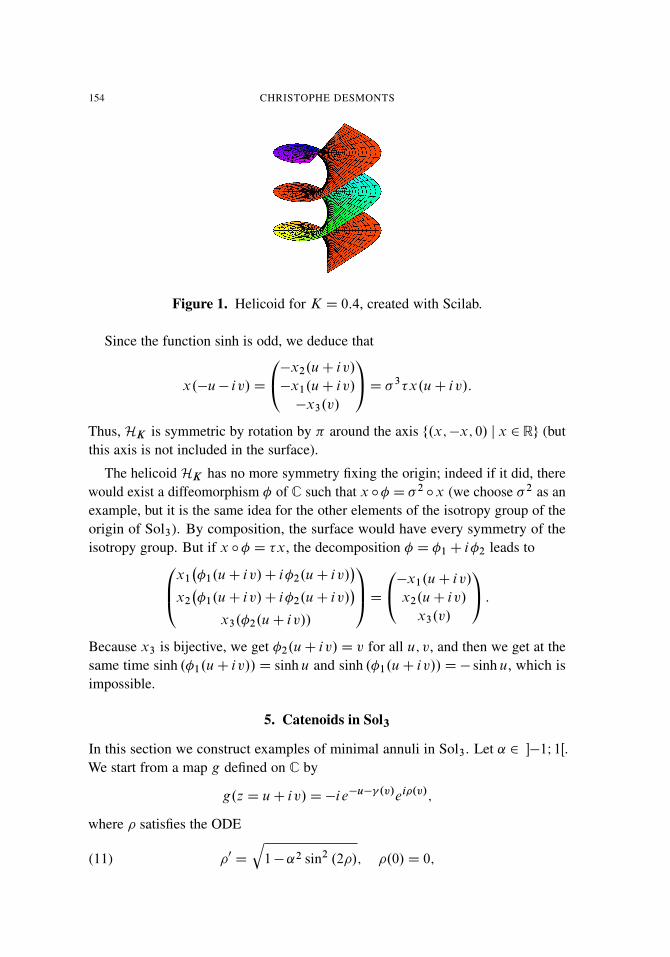
154 CHRISTOPHE DESMONTS
Figure 1. Helicoid for K D 0:4, created with Scilab.
Since the function sinh is odd, we deduce that
x.�u� iv/D
0@�x2.uC iv/
�x1.uC iv/
�x3.v/
1AD �3�x.uC iv/:
Thus, HK is symmetric by rotation by � around the axis f.x;�x; 0/ j x 2 Rg (butthis axis is not included in the surface).
The helicoid HK has no more symmetry fixing the origin; indeed if it did, therewould exist a diffeomorphism � of C such that x ı� D �2 ıx (we choose �2 as anexample, but it is the same idea for the other elements of the isotropy group of theorigin of Sol3). By composition, the surface would have every symmetry of theisotropy group. But if x ı� D �x, the decomposition � D �1C i�2 leads to0B@x1
��1.uC iv/C i�2.uC iv/
�x2
��1.uC iv/C i�2.uC iv/
�x3.�2.uC iv//
1CAD0@�x1.uC iv/
x2.uC iv/
x3.v/
1A :Because x3 is bijective, we get �2.uC iv/D v for all u; v, and then we get at thesame time sinh .�1.uC iv//D sinh u and sinh .�1.uC iv//D� sinh u, which isimpossible.
5. Catenoids in Sol3
In this section we construct examples of minimal annuli in Sol3. Let ˛ 2 ��1I 1Œ.We start from a map g defined on C by
g.z D uC iv/D�ie�u� .v/ei�.v/;
where � satisfies the ODE
(11) �0 D
q1�˛2 sin2 .2�/; �.0/D 0;
PERIODIC MINIMAL SURFACES AND MINIMAL ANNULI IN SOL3 155
and is defined by
(12) 0 D�˛ sin .2�/; .0/D 0:
Proposition 11. The map � is well-defined and has the following properties:
(1) The function � is an increasing diffeomorphism from R onto R.
(2) The function � is odd.
(3) There exists a real number V > 0 such that
8v 2 R; �.vCV /D �.v/C�:
(4) The function � satisfies �.kV /D k� for all k 2 Z.
Proof. Since ˛ 2 ��1; 1Œ , there exists r > 0 such that 1�˛2 sin2 .2�/ 2 �r; 1�; theCauchy–Lipschitz theorem can be applied, and � is well-defined. By (11) we have�0 > 0 on its domain of definition, and
pr < �0 < 1. Since �0 is bounded by two
positive constants, � is defined on R, and
limv!˙1
�.v/D˙1:
The function O� W v 7! ��.�v/ satisfies (11) with O�.0/ D 0; hence O� D � and� is odd. Finally, there exists V > 0 such that �.V / D �; Then the functionQ� W v 7! �.vCV /�� satisfies (11) with Q�.0/D 0; hence Q�D �. �
Corollary 12. (1) We have �.kV =2/D k�=2 for all k 2 2ZC 1.
(2) We have �.�vCV =2/D��.v/C �2
for all v 2R. In particular, �.V =4/D �4
and �.3V =4/D 3�4
.
Proof. (1) We have
��
V
2
�D �
��
V
2CV
�D��
�V
2
�C�;
which gives the formula for k D 1, and part (1) easily follows.
(2) The functions �� W v 7! �=2� �.�vCV =2/ and � satisfy equation (11) with��.0/D �.0/D 0, so �� D � and
�.V =4/D ��.V =4/D �2� �
��2��4
�;
and the result follows. �
Proposition 13. The function g satisfies .g2 � Ng2/gz Nz D 2ggzgNz , and its Hopf
differential is
(13) QD�˛
4dz2:
156 CHRISTOPHE DESMONTS
Proof. A direct calculation shows that g satisfies the equation. Hence, the Hopfdifferential is given by
zQDi.1� �02� 02� 2i 0/
8 sin .2�/dz2D�
˛
4dz2: �
Thus the map g induces a conformal minimal immersion x D .x1;x2;x3/
such that
x1z D e�x3. Ng2� 1/gz
g2� Ng2; x2z D iex3
. Ng2C 1/gz
g2� Ng2; x3z D
2 Nggz
g2� Ng2:
This application is an immersion since the metric induced by x is given by
dw2D kxuk
2jdzj2
D .F 02C˛2/ cosh2 .uC /jdzj2
D
�˛4 sin2 .2�/
.1C �0/2C˛2
�cosh2 .uC /jdzj2
D2˛2
1C �0cosh2 .uC /jdzj2:
In particular,
x3z Di�0� 0� i
2 sin .2�/;
that is, 8<ˆ:
x3u D 2<.x3z/D� 0
sin .2�/D ˛;
x3v D�2=.x3z/D1� �0
sin .2�/D˛2 sin .2�/
1C �0:
Thus
x3.uC iv/D ˛uC˛2
Z v sin .2�.s//1C �0.s/
ds:
Here we have to choose an initial condition; we set
F.v/D ˛2
Z v
0
sin .2�.s//1C �0.s/
ds;
and definex3.uC iv/D ˛uCF.v/:
The function F is well-defined on R.
Proposition 14. The function F is even and V -periodic.
PERIODIC MINIMAL SURFACES AND MINIMAL ANNULI IN SOL3 157
Proof. The function F 0 is odd because � is odd and �0 is even, so F is even. Thenwe get
F 0.vCV /D ˛2 sin .2�.v/C 2�/
1C �0.v/D F 0.v/;
so there exists a constant C such that F.vC V / D F.v/C C for all v 2 R. Byevaluating at zero, we get C D F.V /, that is,
C D ˛2
Z V
0
sin .2�.s//1C �0.s/
ds D ˛2
Z V
0
H.s/ ds
D ˛2
�Z V =4
0
H.s/ dsC
Z 3V =4
V =4
H.s/ dsC
Z V
3V =4
H.s/ ds
�
WD
2XkD0
Lk.˛/:
We can now do the change of variable uD sin .2�.s// in each integral Lk.˛/, with
duD 2�0.s/ cos .2�.s// ds D 2.�1/kq.1�˛2u2/.1�u2/ ds:
Thus,
C D ˛2
Z 1
�1
u du
.1Cp
1�˛2u2/p.1�˛2u2/.1�u2/
D 0
and F is V -periodic. �
Proposition 15. The function is even and V -periodic.
Proof. We prove the proposition in exactly the same way as for the function F . �
The two other equations become
x1z D e�x3.e�u� �i�C euC Ci�/.1� �0� i 0/
4 sin .2�/;
x2z D�ex3.euC Ci� � e�u� �i�/.i � i�0C 0/
4 sin .2�/:
Those equations lead to
x1 D e�˛u�F
�euC
2.1�˛/.F 0 cos ��˛ sin �/�
e�u�
2.1C˛/.˛ sin �CF 0 cos �/
�;
x2 D e˛uCF
��euC
2.1C˛/.˛ cos �CF 0 sin �/C
e�u�
2.˛� 1/.˛ cos ��F 0 sin �/
�:
Remark. If ˛ D 0, then x.C/D f0g. This case will be excluded in the sequel.

158 CHRISTOPHE DESMONTS
Theorem 16. Let ˛ be a real number such that j˛j< 1 and ˛¤ 0, and � and thefunctions defined by (11) and (12). We define the function F by
F.v/D ˛2
Z v
0
sin .2�.s//1C �0.s/
ds:
Then the map x W C! Sol3 defined by0BBBBB@e�˛u�F
�euC
2.1�˛/.F 0 cos ��˛ sin �/�
e�u�
2.1C˛/.˛ sin �CF 0 cos �/
�e˛uCF
��euC
2.1C˛/.˛ cos �CF 0 sin �/C
e�u�
2.˛� 1/.˛ cos ��F 0 sin �/
�˛uCF
1CCCCCAis a conformal minimal immersion whose Gauss map is
g W uC iv 2 C 7�! �ie�u� .v/ei�.v/:
Moreover,
(14) x.uC i.vC 2V //D x.uC iv/
for all u; v 2R. The surface given by x is called a catenoid of parameter ˛ and willbe denoted by C˛.
Proof. The periodicity of C˛ is an application of Propositions 11, 14 and 15. �
Remark. The surfaces C˛ and C�˛ are related; if we denote by the indices ˛ and�˛the data describing C˛ and C�˛, we get8<:
��˛ D �˛;
F�˛D F˛;
�˛ D� ˛:
Thus, we getx�˛.�uC iv/D �2x˛.uC iv/:
In particular, there exists an orientation-preserving isometry of Sol3 fixing the originthat sends C˛ on C�˛.
Now we show that the catenoids are embedded:
Proposition 17. For all � 2 R, the intersection of C˛ with the plane fx3 D �g is anonempty closed embedded convex curve.
Proof. This intersection is nonempty: x.�=˛C i0/ 2 C˛ \ fx3 D �g. We look atthe curve in C defined by x3.uC iv/D ˛uCF.v/D �, i.e., the curve
c W t 2 R 7�!
���F.t/
˛; t�:
PERIODIC MINIMAL SURFACES AND MINIMAL ANNULI IN SOL3 159
Its image by x is
c W t 2R 7�!
0BBBBBB@e��
�eıC
2.1�˛/.F 0 cos��˛ sin�/�
e�ı�
2.1C˛/.˛ sin�CF 0 cos�/
�
e���eıC
2.1C˛/.˛ cos�CF 0 sin�/C
e�ı�
2.˛�1/.˛ cos��F 0 sin�/
�c
1CCCCCCA.t/;
where ı D ��F˛
. The calculation leads to
c01.t/De��
˛.1�˛2/
�A.t/ cosh
���F
˛C
�CB.t/ sinh
���F
˛C
��;
with8<ˆ:
AD�F 02 cos �C˛ 0F 0 cos ��˛2�0 cos �C˛2F 0 sin ��˛3 0 sin �
C˛2F 00 cos ��˛2F 0�0 sin �;
B D ˛F 0 sin ��˛2 0 sin �C˛F 00 cos ��˛F 0�0 sin ��˛F 02 cos �
C˛2 0F 0 cos ��˛3�0 cos �:
We remark that B � 0 after simplifications, and
A.t/D .F 02.t/C˛2/.˛2� 1/ cos �.t/:
Finally,
c01.t/D�e��
˛.F 02.t/C˛2/ cos �.t/ cosh
���F.t/
˛C .t/
�:
In the same way, we get
c02.t/D�e��
˛.F 02.t/C˛2/ sin �.t/ cosh
���F.t/
˛C .t/
�:
Thus
c021 C c022 De�2�
˛2.F 02.t/C˛2/2 cosh2
���F.t/
˛C .t/
�> 0;
so the intersection C˛ \ fx3 D �g is a smooth curve; moreover, it’s closed sincec.t C 2V /D c.t/ for all t 2 R.
The planes fx3 D �g are flat: indeed, the metrics on these planes are e2�dx21C
e�2�dx22
, so up to an affine transformation, we can work in euclidean coordinates,as we suppose in this proof since affinities preserve convexity.
To prove that c is embedded and convex, we consider the part of c corresponding tot 2 .�V =2;V =2/. On .�V =2;V =2/, we have cos �.t/>0, thanks to Proposition 11
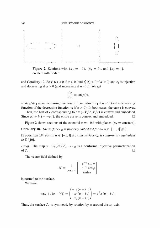
160 CHRISTOPHE DESMONTS
Figure 2. Sections with fx3 D �1g, fx3 D 0g, and fx3 D 1g,created with Scilab.
and Corollary 12. So c01.t/ < 0 if ˛ > 0 (and c0
1.t/ > 0 if ˛ < 0) and c1 is injective
and decreasing if ˛ > 0 (and increasing if ˛ < 0). We get
dc2
dc1
D tan �.t/;
so dc2=dc1 is an increasing function of t , and also of c1 if ˛ < 0 (and a decreasingfunction of the decreasing function c1 if ˛ > 0). In both cases, the curve is convex.
Then, the half of c corresponding to t 2 .�V =2;V =2/ is convex and embedded.Since c.t CV /D�c.t/, the entire curve is convex and embedded. �
Figure 2 shows sections of the catenoid ˛ D�0:6 with planes fx3 D constantg.
Corollary 18. The surface C˛ is properly embedded for all ˛ 2 ��1; 1Œnf0g.
Proposition 19. For all ˛ 2 ��1; 1Œnf0g, the surface C˛ is conformally equivalentto C nf0g.
Proof. The map x W C=.2iV Z/ ! C˛ is a conformal bijective parametrizationof C˛. �
The vector field defined by
N D1
cosh u
24 e� sin ��e� cos �
sinh u
35is normal to the surface.
We have
x.uC i.vCV //D
0@�x1.uC iv/
�x2.uC iv/
x3.uC iv/
1AD �2x.uC iv/:
Thus, the surface C˛ is symmetric by rotation by � around the x3-axis.

PERIODIC MINIMAL SURFACES AND MINIMAL ANNULI IN SOL3 161
Figure 3. Catenoid for ˛ D�0:6, created with Scilab.
Remark. The x3-axis is contained in the “interior” of C˛ since each curveC˛ \fx3 D �g is convex and symmetric with respect to this axis.
We also get
x.u� iv/D
0@�x1.uC iv/
x2.uC iv/
x3.uC iv/
1AD �x.uC iv/;
and the surface C˛ is symmetric by reflection in the plane fx1 D 0g, and finally wehave
x.uC i.�vCV //D �2�x.uC iv/;
and C˛ is symmetric by reflection in the plane fx2 D 0g.
If C˛ had another symmetry fixing the origin, it would have every symmetry ofthe isotropy group of Sol3, and we prove as for the helicoid that it is impossible.
6. Limits of catenoids
6.1. The case ˛ D 0. In this part we consider the limit surface of the catenoids C˛when ˛ goes to zero. For this, we do the change of parameters(
u0 D uC ln˛;
v0 D v:
In these coordinates, the immersion x given in Theorem 16 takes the form0BBBBBB@e˛ ln˛�˛u0�F
�eu0C
2˛.1�˛/.cos�F 0�˛ sin�/�
˛e�u0�
2.1C˛/.˛ sin�Ccos�F 0/
�
e�˛ ln˛C˛u0CF
��eu0C
2˛.1C˛/.˛ cos�CF 0 sin�/C
˛e�u0�
2.˛�1/.˛ cos��F 0 sin�/
��˛ ln˛C˛u0CF
1CCCCCCA :
162 CHRISTOPHE DESMONTS
Letting ˛ go to zero, we get 8<ˆ:
� �! Id;
F=˛ �! 0;
F 0=˛ �! 0;
�! 0;
and so the limit immersion is 0BBBBB@�
eu0
2sin v0
�eu0
2cos v0
0
1CCCCCA :Thus, we obtain a parametrization of the plane fx3 D 0g, which is the limit of thefamily .C˛/ when ˛! 0.
6.2. The case ˛ D 1. We end by the study of the case ˛ D 1 (the case ˛ D�1 isexactly the same). We show that the limit surface is a minimal entire graph:
Proposition 20. Let x W R2! Sol3 be defined by
x.uC iv/D
0@x1
x2
x3
1AD0BBBBB@�
tanh v2
.1C e�2u/
e2u
4�
u
2�
cosh .2v/4
uC ln .cosh v/
1CCCCCA :Then x is a minimal immersion and there exists a C1-function f defined on R2
such that the image of x (called S) is the x2-graph of f given by x2 D f .x1;x3/.
Proof. We show that this surface is (up to a translation) the limit surface of thefamily .C˛/˛2��1;1Œ when ˛ goes to 1. For ˛ D 1, the Gauss map is still given byg.z D uC iv/D�ie�u� .v/ei�.v/, but � satisfies the ODE
(15) �0 D cos .2�/; �.0/D 0;
and is still defined by
(16) 0 D� sin .2�/; .0/D 0:
We have explicit expressions for these functions, which are given by
�.v/D arctan e2v��=4D arctan .tanh v/;
.v/D�12
ln .cosh .2v//:
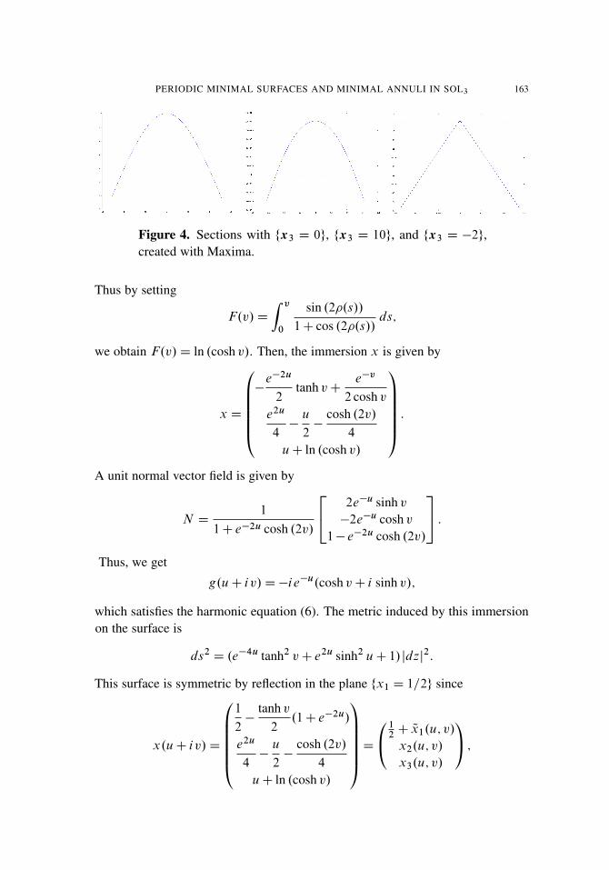
PERIODIC MINIMAL SURFACES AND MINIMAL ANNULI IN SOL3 163
Figure 4. Sections with fx3 D 0g, fx3 D 10g, and fx3 D �2g,created with Maxima.
Thus by setting
F.v/D
Z v
0
sin .2�.s//1C cos .2�.s//
ds;
we obtain F.v/D ln .cosh v/. Then, the immersion x is given by
x D
0BBBBB@�
e�2u
2tanh vC
e�v
2 cosh ve2u
4�
u
2�
cosh .2v/4
uC ln .cosh v/
1CCCCCA :
A unit normal vector field is given by
N D1
1C e�2u cosh .2v/
24 2e�u sinh v�2e�u cosh v
1� e�2u cosh .2v/
35 :Thus, we get
g.uC iv/D�ie�u.cosh vC i sinh v/;
which satisfies the harmonic equation (6). The metric induced by this immersionon the surface is
ds2D .e�4u tanh2 vC e2u sinh2 uC 1/jdzj2:
This surface is symmetric by reflection in the plane fx1 D 1=2g since
x.uC iv/D
0BBBBB@1
2�
tanh v2
.1C e�2u/
e2u
4�
u
2�
cosh .2v/4
uC ln .cosh v/
1CCCCCAD0@1
2C Qx1.u; v/
x2.u; v/
x3.u; v/
1A ;
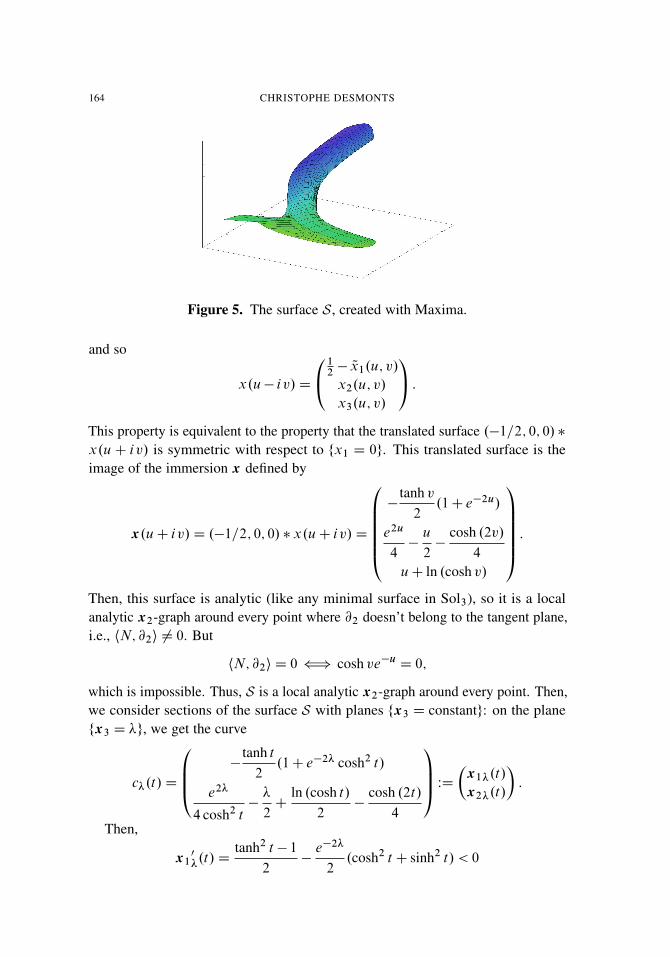
164 CHRISTOPHE DESMONTS
Figure 5. The surface S, created with Maxima.
and so
x.u� iv/D
0@12� Qx1.u; v/
x2.u; v/
x3.u; v/
1A :This property is equivalent to the property that the translated surface .�1=2; 0; 0/�
x.uC iv/ is symmetric with respect to fx1 D 0g. This translated surface is theimage of the immersion x defined by
x.uC iv/D .�1=2; 0; 0/�x.uC iv/D
0BBBBB@�
tanh v2
.1C e�2u/
e2u
4�
u
2�
cosh .2v/4
uC ln .cosh v/
1CCCCCA :Then, this surface is analytic (like any minimal surface in Sol3), so it is a localanalytic x2-graph around every point where @2 doesn’t belong to the tangent plane,i.e., hN; @2i ¤ 0. But
hN; @2i D 0 ” cosh ve�uD 0;
which is impossible. Thus, S is a local analytic x2-graph around every point. Then,we consider sections of the surface S with planes fx3 D constantg: on the planefx3 D �g, we get the curve
c�.t/D
0BB@ �tanh t
2.1C e�2� cosh2 t/
e2�
4 cosh2 t��
2C
ln .cosh t/
2�
cosh .2t/
4
1CCA WD �x1�.t/
x2�.t/
�:
Then,
x10�.t/D
tanh2 t � 1
2�
e�2�
2.cosh2 t C sinh2 t/ < 0
PERIODIC MINIMAL SURFACES AND MINIMAL ANNULI IN SOL3 165
for all t 2R. Thus, the curves are injective, so the surface S is embedded. Moreover,by the implicit function theorem, we deduce that for every � 2 R, there exists afunction f� such that x2� D f�.x1�/. Because the function x1� is a decreasingdiffeomorphism of R, the function f� is defined on R. This calculus is valid forall � 2 R, so there exists a function f W R2! R such that x2 D f .x1;x3/.
Finally, this function f coincides around every point with the local C1-functionswhich give the local graphs, and so f is C1. �
As a conclusion, we can notice that, for a fixed x3,
� when x1!C1, x2 ��x1e2x3 ;
� when x1!�1, x2 � x1e2x3 .
References
[Abresch and Rosenberg 2004] U. Abresch and H. Rosenberg, “A Hopf differential for constant meancurvature surfaces in S2
�R and H2 �R”, Acta Math. 193:2 (2004), 141–174. MR 2006h:53003Zbl 1078.53053
[Abresch and Rosenberg 2005] U. Abresch and H. Rosenberg, “Generalized Hopf differentials”, Mat.Contemp. 28 (2005), 1–28. MR 2006h:53004 Zbl 1118.53036
[Berdinskii and Taimanov 2005] D. A. Berdinskii and I. A. Taimanov, “Poverhnosti v trehmer-nyh pruppah Li”, Sibirsk. Mat. Zh. 46:6 (2005), 1248–1264. Translated as “Surfaces in three-dimensional Lie groups” in Sib. Math. J. 46:6 (2005), 1005–1019. MR 2006j:53087 Zbl 1117.53045
[Daniel and Hauswirth 2009] B. Daniel and L. Hauswirth, “Half-space theorem, embedded minimalannuli and minimal graphs in the Heisenberg group”, Proc. Lond. Math. Soc. .3/ 98:2 (2009),445–470. MR 2009m:53018 Zbl 1163.53036
[Daniel and Mira 2013] B. Daniel and P. Mira, “Existence and uniqueness of constant mean curvaturespheres in Sol3”, J. Reine Angew. Math. 685 (2013), 1–32. MR 3181562 Zbl 06245199
[Inoguchi and Lee 2008] J.-I. Inoguchi and S. Lee, “A Weierstrass type representation for minimal sur-faces in Sol”, Proc. Amer. Math. Soc. 136:6 (2008), 2209–2216. MR 2008k:53016 Zbl 1157.53007
[López 2014] R. López, “Invariant surfaces in Sol3 with constant mean curvature and their computergraphics”, Adv. Geom. 14:1 (2014), 31–48. MR 3159090 Zbl 1283.53058
[López and Munteanu 2011] R. López and M. I. Munteanu, “Surfaces with constant mean cur-vature in Sol geometry”, Differential Geom. Appl. 29:S1 (2011), S238–S245. MR 2012k:53016Zbl 1250.53058
[López and Munteanu 2012] R. López and M. I. Munteanu, “Minimal translation surfaces in Sol3”, J.Math. Soc. Japan 64:3 (2012), 985–1003. MR 2965436 Zbl 1254.53033
[López and Munteanu 2014] R. López and M. I. Munteanu, “Invariant surfaces in the homoge-neous space Sol with constant curvature”, Math. Nachr. 287:8-9 (2014), 1013–1024. MR 3219227Zbl 1293.53076
[Masaltsev 2006] L. A. Masaltsev, “Minimal surfaces in standard three-dimensional geometry Sol3”,Zh. Mat. Fiz. Anal. Geom. 2:1 (2006), 104–110. MR 2006j:53008 Zbl 1144.53016
[Meeks and Pérez 2012] W. H. Meeks, III and J. Pérez, “Constant mean curvature surfaces in metricLie groups”, pp. 25–110 in Geometric analysis: partial differential equations and surfaces (Granada,2010), edited by J. Pérez and J. A. Gálvez, Contemporary Mathematics 570, American MathematicalSociety, Providence, RI, 2012. MR 2963596 Zbl 1267.53006
166 CHRISTOPHE DESMONTS
[Menezes 2014] A. Menezes, “Periodic minimal surfaces in semidirect products”, J. Aust. Math. Soc.96:1 (2014), 127–144. MR 3177813 Zbl 1288.53052
[Nguyen 2014] M. H. Nguyen, “The Dirichlet problem for the minimal surface equation in Sol3 withpossible inifinite boundary data”, preprint, 2014. arXiv 1312.6194
Received January 22, 2014. Revised August 1, 2014.
CHRISTOPHE DESMONTS
INSTITUT ELIE CARTAN DE LORRAINE
UNIVERSITÉ DE LORRAINE
B.P. 7023954506 VANDOEUVRE-LÈS-NANCY CEDEX
FRANCE

PACIFIC JOURNAL OF MATHEMATICSVol. 276, No. 1, 2015
dx.doi.org/10.2140/pjm.2015.276.167
QUASI-EXCEPTIONAL DOMAINS
ALEXANDRE EREMENKO AND ERIK LUNDBERG
Exceptional domains are domains on which there exists a positive harmonicfunction, zero on the boundary and such that the normal derivative onthe boundary is constant. Recent results classify (under some mild addi-tional assumptions) exceptional domains as belonging to either a certainone-parameter family of simply periodic domains or one of its scaling limits.
We introduce quasi-exceptional domains by allowing the boundary val-ues to be different constants on each boundary component. This relaxeddefinition retains the interesting property of being an arclength quadraturedomain, and also preserves the connection to the hollow vortex problem influid dynamics. We give a partial classification of such domains in terms ofcertain abelian differentials. We also provide a new two-parameter familyof periodic quasi-exceptional domains. These examples generalize the hol-low vortex array found by Baker, Saffman, and Sheffield. A degenerationof regions of this family provides doubly connected examples.
1. Introduction
A domain D ∈ Rn is called exceptional if there is a positive function u (called aroof function) harmonic in D, zero on the boundary, and with
(1) ∂
∂nu(z)= 1, z ∈ ∂D,
where the differentiation is along the normal pointing inwards into D and it isassumed that the boundary is smooth. Evident examples are exteriors of balls andhalf-spaces. For n > 2, the only other known examples are cylinders whose baseis an exceptional domain in R2. If the smoothness assumption on the boundary isdropped, then there are also certain cones in higher dimensions and pathological“non-Smirnov” examples in the plane [Khavinson et al. 2013].
The problem of describing of all exceptional domains in the plane was stated in[Hauswirth et al. 2011] and settled in [Khavinson et al. 2013] under a topological
Supported by NSF grant DMS-1361836.MSC2010: primary 30C20, 35R35; secondary 76B47, 31A05.Keywords: quadrature domains, hollow vortices, elliptic functions, abelian differentials.
167

168 ALEXANDRE EREMENKO AND ERIK LUNDBERG
assumption which was removed in [Traizet 2014a] using an unexpected correspon-dence with minimal surfaces. The first nontrivial example was given in [Hauswirthet al. 2011]. This example appeared in another context, related to fluid dynamics, in[Longuet-Higgins 1988]. A second nontrivial example was noticed in [Khavinsonet al. 2013] and [Traizet 2014a]. This example had also appeared previously instudies of fluid dynamics [Baker et al. 1976] (see also [Crowdy and Green 2011]).
Let us introduce quasi-exceptional domains, by relaxing the definition to allowthe Dirichlet condition to be a different constant on each boundary component.Thus, a domain D ∈ Rn is called quasi-exceptional if there is a positive harmonicfunction u in D which is constant on each boundary component (but not necessarilythe same constant) and the Neumann condition (1) holds. We will continue tocall u a roof function. Again, we assume that each component of the boundaryis smooth.
Added in press: In an interesting preprint, Martin Traizet [2014b] has consideredan even more general problem, allowing the Neumann data to take different signson different components. As with the current paper, that work is motivated bythe hollow vortex problem from fluid dynamics. Extending [Traizet 2014a], acorrespondence to minimal surfaces is given in that work, and techniques fromminimal surface theory are used to produce new examples.
We summarize several interesting aspects of exceptional domains. These state-ments all hold true for quasi-exceptional domains.
• Fluid dynamics: As noted above, the two nontrivial examples first appeared influid dynamics [Longuet-Higgins 1988; Baker et al. 1976]. In general, one caninterpret exceptional domains in terms of a hollow vortex problem. The levellines of u can be interpreted as stream lines of a two-dimensional stationaryflow of ideal fluid, and condition (1) expresses the fact that the pressure isconstant on the boundary. Such conditions may exist if the components of thecomplement of D are air bubbles in the surrounding liquid. Notice that therotation of the fluid around all bubbles corresponding to exceptional domainsis in the same direction because ∂u/∂n > 0 on the boundary.
• Quadrature domains [Gustafsson 1987]: Exceptional domains provide exam-ples of arclength null-quadrature domains, that is, domains for which integralswith respect to arclength over ∂D of every analytic function in the Smirnovclass E1(D) vanish.
• Differentials on Riemann surfaces: By way of the connection to quadraturedomains, the study [Gustafsson 1987] indicates a connection to half-orderdifferentials. We make use of abelian differentials in Section 4 below.
QUASI-EXCEPTIONAL DOMAINS 169
• The Schwarz function of a curve: In [Khavinson et al. 2013], it was noticedthat the function u(z) satisfies
∂zu(z)=√−S′(z),
where S(z) is the Schwarz function of ∂� and ∂z =12(∂x− i∂y) is the Cauchy–
Riemann operator.
• Minimal surfaces: Traizet [2014a] established a nontrivial correspondencebetween exceptional domains and a special type of minimal surfaces called“minimal bigraphs”. In [Traizet 2014b], this correspondence was extended toquasi-exceptional domains, but the minimal surfaces in that case need not beembedded. This prevents applying the results on complete embedded minimalsurfaces that were used in [Traizet 2014a] to classify exceptional domains.
The classification results for exceptional domains of finite connectivity showthat they are quite restricted; all examples can be conformally mapped onto a diskby elementary functions.
Problem A. Classify quasi-exceptional domains.
We begin to address this problem below, give a partial classification of periodicand finitely connected exceptional domains, and provide new periodic and doublyconnected examples described in terms of elliptic functions. First, we explain therelation to arclength null-quadrature domains.
2. Arclength null-quadrature domains
A bounded domain D ⊂C is a quadrature domain if it admits a formula expressingthe area integral of every function f analytic and integrable in D as a finite sum ofweighted point evaluations of the function and its derivatives, i.e.,
(2)∫
Dg(z) dA(z)=
N∑m=1
nm∑k=0
am,k g(k)(zm),
where the zm are distinct points in D and the am,k are constants independent of g.A (necessarily unbounded) domain D ⊂ C is called a null-quadrature domain
(NQD) if the area integral of every function g analytic and integrable in D vanishes:
(3)∫
Dg(z) dA(z)= 0.
M. Sakai [1981] completely classified NQDs in the plane.Following [Khavinson et al. 2013], we refer to a domain D ⊂ C as an arclength
null-quadrature domain (ALNQD) if the integral over ∂D of every function g in

170 ALEXANDRE EREMENKO AND ERIK LUNDBERG
the Smirnov class E1(D) vanishes (in the case∞ is an isolated point on ∂D, wetake the restricted class of functions g(z) ∈ E1(D) vanishing at infinity):
(4)∫∂D
g(z) ds(z)= 0.
The Smirnov class E1(D) is not the same as the Hardy space H 1(D). Namely,a function g analytic in D is said to belong to E1(D) if there exists a sequence ofdomains D1⊂D2⊂· · · , with
⋃k Dk=D, and with rectifiable boundaries, such that:
supk
∫∂Dk
|g(z)| |dz|<∞.
One may also define quadrature domains in higher dimensions using a test class ofharmonic functions, but we will restrict ourselves to the case of n = 2 dimensions.
Inspired by the successful classification of NQDs [Sakai 1981], the problem ofclassifying ALNQDs was suggested in [Khavinson et al. 2013]. We pose this prob-lem again while stressing that it does not reduce to the classification of exceptionaldomains (whereas it might reduce to classification of quasi-exceptional domains).
Problem B. Classify ALNQDs.
The following proposition shows that quasi-exceptional domains are ALNQDs.Thus, the new examples (described in the last section) of quasi-exceptional domainsalso provide new ALNQDs. Problem B is closely related to Problem A, and if theconverse of the proposition is true then the two problems are equivalent.
Proposition 1. If D is a quasi-exceptional domain, then D is an ALNQD.
Proof. Consider the complex analytic function F(z)= ux− iu y , where u is the rooffunction. We will need the following claim, which is proved in the next section(see Lemma 2).
Claim. The roof function u of D satisfies ∇u(z)= O(1) in D, so F(z) is bounded.
Suppose that g is in the Smirnov space E1(D). Using the fact that ds= i F(z) dz,
(5)∫∂D
g(z) ds =∫∂D
ig(z)F(z) dz.
As F is bounded, gF ∈ E1(D). If∞ is not an isolated boundary point, then theintegral equals zero by Cauchy’s theorem.
If∞ is an isolated boundary point, then we have u(z)= log|z|+const+O(1/z),so F(z)= O(1/z), z→∞. Now g(∞)= 0, so Fg has a zero of order at least 2at∞, and the integral is zero again. �

QUASI-EXCEPTIONAL DOMAINS 171
3. A potential theoretic restriction on the roof function
We restrict ourselves to the case n = 2, and assume that the order of connectivity ofD is finite, or that the roof function u is periodic and a fundamental region for Dhas finite connectivity.
Recall that a Martin function is a positive harmonic function M in a domain� with the property that for any positive harmonic function v in � the conditionv ≤ M implies that v = cM , where c > 0 is a constant. (Often, Martin functionsare called minimal harmonic functions — see [Heins 1950].) Martin functions onfinitely connected domains are simply Poisson kernels evaluated at points of theMartin boundary, the boundary under Carathéodory compactification (prime ends)of the domain (see [Brelot 1971]).
Any domain D of finite connectivity in C is conformally equivalent to a circulardomain �. A circular domain is a domain whose boundary components are pointsor circles. For a circular domain, a Martin function M can be of two types:
(a) There is a component of ∂� which is a single point z0, and M is proportionalto the Green function of �∪ {z0} with the singularity at z0.
(b) There is a point z0 ∈ ∂� which is not a component of ∂�, and M has boundaryvalue zero at all points of ∂� \ {z0}. The local behavior in this case is like− Im(1/z) in the upper half-plane near 0.
Let D be an exceptional domain, and u a harmonic function with the property (1).The following result was proved for exceptional domains by the current first author,but was communicated in [Khavinson et al. 2013, Theorem 4.2]. Here we repeatthe proof with minor adjustments.
Lemma 2. The roof function u of a quasi-exceptional domain satisfies the equation∇u(z)= O(1) in D. Moreover, u is the sum of a bounded harmonic function andat most two Martin functions.
Proof. We follow the second part of the proof from [Khavinson et al. 2013]. LetR > 0, and consider an auxiliary function
wR =|∇u|
u+ R.
A direct computation shows that
(6) 1 logwR = w2R,
and wR(z)= 1/(ck + R)≤ 1/R for z ∈ ∂D, where ck ≥ 0 are the constants takenin the Dirichlet condition. We claim that
(7) wR(z)≤ 2/R, z ∈ D,
172 ALEXANDRE EREMENKO AND ERIK LUNDBERG
from which the result follows by letting R→∞, which gives |∇u| ≤ 2 in D.Suppose, contrary to (7), that wR(z0) > 2/R for some z0 ∈ D. Let
v(z)=2R
R2− |z− z0|2, z ∈ B(z0, R)= {z : |z− z0|< R}.
Obviously, v(z)≥ 2/R. A computation reveals that 1 log v = v2. Let
K = {z ∈ D ∩ B(z0, R) : wR(z) > v(z)}.
We have z0 ∈ K , since v(z0)= 2/R. Let K0 be the component of K containing z0.Then we have wR(z)= v(z) on ∂K0, since wR(z) < v(z) on ∂D ∩ B(z0, R) whilev(z)=+∞ on ∂B(z0, R). On the other hand,
1(logwR − log v)= w2R − v
2 > 0 in K0.
So the subharmonic function logwR − log v is positive in K0 and vanishes on theboundary — a contradiction.
This proves that ∇u = O(1). In order to see the second statement, we notethat ∇u = O(1) implies that u(z) = O(|z|) has order 1. The result then followsby first solving the Dirichlet problem (with a bounded function) having the sameboundary values as u; subtracting this function, one may then apply [Kjellberg1950, Theorem II]. �
4. Partial classification in terms of abelian differentials
Let D be a QE domain of one of the following types:
Type I: D is finitely connected.
Type II: D/0 is finitely connected, where 0 is the group of transformationsz 7→ z+ nω, and u(z+ω)= u(z) for some ω ∈ C \ {0}. We call this theperiodic case. (As above, u is the roof function.)
In this section we give a classification of QE domains of these two types interms of abelian differentials of a compact Riemann surface with an anticonformalinvolution.
If D is of type I, and∞ is an isolated boundary point, then D′ = D ∪ {∞} isconformally equivalent to some bounded circular domain �, and we suppose thatp ∈� corresponds to∞. If∞ is not isolated, we put D′ = D, and � is a boundedcircular domain conformally equivalent to D′. In any case, we have a conformalmap φ :�→ D′, which may have at most one simple pole at p ∈�.
If D is of type II, let G = D/0. The Riemann surface G is a finitely connecteddomain on the cylinder C/0; this cylinder is conformally equivalent to the puncturedplane, and we identify it with C∗. Then G ⊂ C∗ must have one or two puncturesof C/0 as isolated boundary points, and we denote by G ′ the union of G with

QUASI-EXCEPTIONAL DOMAINS 173
these isolated boundary points. Then G ′ is conformally equivalent to a boundedcircular domain of finite connectivity � in which there are one or two points a andb corresponding to the added punctures. We have a multivalued conformal mapφ :�→ D.
The points a and b are logarithmic singularities of φ.We pull back u on �; i.e., set v = u ◦φ. As u is periodic, v is a single-valued
positive harmonic function on � \ {a, b}. Consider the differential on �
dv = vz dz = 12(vx − ivy)(dx + idy)= g(z) dz.
This is well-defined on �: g is a single-valued meromorphic function in � withat most simple poles at p or a and b. Indeed, for a positive harmonic function,an isolated singularity is either removable or logarithmic. In the second case thegradient has a simple pole.
Next, we extend v as a multivalued function to a compact Riemann surface S.Let �′ be the mirror image of �; we glue it to � in the standard way (along eachcircular boundary component) and obtain a compact Riemann surface S. We denoteby σ : z 7→ z∗ the anticonformal involution which fixes the boundary componentsof �. The Riemann surface S is of genus g, and the involution σ has fixed setcorresponding to ∂�, which consists of n = g+1 ovals. Such involutions are calledinvolutions of maximal type, meaning that the complement of the fixed set of theinvolution consists of two regions homeomorphic to planar regions.
Each branch of v is constant on each boundary component, so it extends throughthis boundary component by reflection to the double S of �. The extensions ofvarious branches of v through different boundary components do not match: theydiffer by additive constants. On the other hand, the differential dv is well-definedon the double. Namely,
(8) (dv)∗ =−dv,
where ∗ is the action of involution on differentials. Thus we have a meromorphicdifferential dv on S.
Choose a basis of 1-homology in S so that the A-loops are simple closed curvesin �, each homotopic to one boundary component of �, and the B loops are dualto the A-loops. For type I, all periods over A-loops are purely imaginary, because
v = Re∫
dv
is single-valued. For type II, these periods are imaginary except those whichcorrespond to simple loops around one pole, a or b.

174 ALEXANDRE EREMENKO AND ERIK LUNDBERG
Now we discuss φ, or better, the differential dφ = φ′(z) dz. We have, from thecondition that our domain is quasi-exceptional,
2|dv| = |dφ| on ∂�.
The ratio of two differentials is a function. So we have a meromorphic function Bon � such that
(9) 2B dv = dφ.
This function has absolute value 1 on ∂�. Therefore, it extends to S by symmetry.It has no zeros in � because dφ has no zeros. Its poles in � must match the zerosof dv, because dφ is zero-free (indeed, φ is univalent). In fact, B is a meromorphicfunction on S. To justify this claim when dv has a singularity on ∂�, we observethat this singularity is removable for B, which follows from the next lemma:
Lemma 3. Consider the equation
φ′ = Bh,
where h is meromorphic in a neighborhood V of 0, B is holomorphic and zero-freein V \ {0}, |B(z)| = 1 for z ∈ V ∩R \ {0}, and φ is univalent in {z ∈ V : Im z > 0}.Then the singularity of B at 0 is removable.
Before proving the lemma, we note that in order to apply it in our setting wecompose B with a linear fractional transformation that sends V to a neighborhoodof the singularity we wish to remove such that the real line is mapped to the circularboundary component with 0 sent to the singularity.
Proof. In order to prove this by contradiction, assume that 0 is an essential singularityof B. By symmetry we have B(z )= 1/B(z). We claim that there exists a sequencezk→ 0 such that
(10) lim infk→∞
∣∣zk log|B(zk)|∣∣> 0.
Indeed, suppose that this is not so. Then log |B(z)| = o(z−1), and the Phragmén–Lindelöf theorem (see, for example, [Levin 1980, Chapter I, Theorem 22]) impliesthat B has a limit as z→ 0. By choosing a subsequence and using symmetry, wecan find a sequence in the upper half-plane with the property
(11) lim infk→∞
|zk | log |B(zk)|> 0,
or with the property
(12) lim infk→∞
|zk | log |B(zk)|< 0.

QUASI-EXCEPTIONAL DOMAINS 175
Distortion theorems for univalent functions imply that
(13) c(Im z)3 ≤ |φ′(z)| ≤ C(Im z)−3.
In addition to this, we have, for some integer m,
(14) c|x |m ≤ |φ′(x)| ≤ C |x |m, z ∈ V ∩R,
because h is meromorphic and |B(x)| = 1 for z ∈ V ∩R. Taking n =max{3,−m},we obtain that the subharmonic function u(z)= log+|znφ′(z)/C | satisfies u(x)= 0for x ∈ V ∩R, and u(reiθ )≤ ψ(θ), where ψ(θ)=−3 log sin θ for θ ∈ (0, π). As∫ π
0ψ(θ) dθ <∞,
we can apply Carleman’s “log log” theorem [Carleman 1926; Rashkovskii 2009],and conclude that u is bounded from above in the intersection of V with the upperhalf-plane. This contradicts (11). If (12) holds, one applies the same argument to1/φ′. This completes the proof of the lemma. �
We can thus restate the problem of finding QE domains (under the restrictionswe impose) as follows:
Proposition 4. All QE domains of types I and II are parametrized by triples(S, dω, B), where S is a compact Riemann surface with an involution of maximaltype, dω is a meromorphic differential that enjoys the symmetry property (8), and Bis a function that has the symmetry property
B∗(z) := B(z∗)= 1/B(z)
and has poles at the zeros of dω on one half of S, that is, in�. There is an additionalcondition: that
(15) φ = 2∫
B dω
is globally univalent and single-valued in type I, and single-valued except theresidues in type II.
To recover D from a triple (S, dw, B), one takes one of the components �⊂ Scomplementary to the fixed set of the involution. Then D = φ(�), where φ isdefined in (15).
In order to check the condition on the global univalence of φ, it is sufficientto verify that periods of dω/B are zero on the boundary curves, and that theseboundary curves are mapped by φ injectively.
The following is a general conclusion:
Proposition 5. The boundary of a quasi-exceptional domain of type I or type II isparametrized by an abelian integral.
176 ALEXANDRE EREMENKO AND ERIK LUNDBERG
Next we provide a partial classification of quasi-exceptional domains in terms ofthe data stated in the above formulation.
Theorem 6. The differential dv has either two or four poles on S, counting multi-plicity. Moreover, if dv has two poles in S, then D is the complement of either adisk or a half-plane.
Remark. If B 6= const, then 1/B is an Ahlfors function of �.
Proof of Theorem 6. Let us first show that dv has some poles. Otherwise, dv isholomorphic, and thus u is bounded. Let z1 ∈ ∂D and z2 ∈ ∂D be the points whereu assumes its maximal and minimal values. Then du/dn has opposite signs at thesetwo points, which contradicts (1).
The differential dv has at most simple poles at p, a, and b (whichever of thesepoints are present) and at their images σ p, σa, and σb. In addition it may havedouble poles on ∂�. The total number of poles (without multiplicity) in� is at mosttwo by Lemma 2. Thus, on S the differential dv has two or four poles, countingmultiplicity.
Notice that v is constant on each boundary component, so the gradient is perpen-dicular to the boundary ∂�, so the total rotation of this gradient as we traverse theboundary is the same as the total rotation of the tangent vector to the boundary.This is equal to 2π(2− n) because the outer boundary component is traversedcounterclockwise and the rest clockwise, as parts of the boundary of �. So vz ,which is conjugate to the gradient, rotates n− 2 times.
From this we can conclude how many zeros dv has in �. The number N of zerosof dv in � satisfies
(16) n− 2= N − (the number of poles in �),
where a double pole on ∂� is counted as a single pole in �. This formula iswell known.
Suppose that dv has exactly two poles, counting multiplicity. This can occur inone of three ways:
Case (1): dv has a simple pole at p in �.
Case (2): dv has one double pole at z0 ∈ ∂�.
Case (3): dv has a simple pole at a in � (and b does not exist).
If Case (1) holds, then∞ is an isolated point on ∂D, and, by Proposition 1, D isan arclength quadrature domain with quadrature point at∞. It now follows from[Gustafsson 1987, Remark 6.1] that D is the exterior of a disk.
In Case (2), we will show that B is constant. First note that dφ has a doublepole at z0, so B does not have a zero or a pole at z0. Since φ is a conformal map, itfollows from (9) that B has no zeros and N poles in � (located at the zeros of dv).

QUASI-EXCEPTIONAL DOMAINS 177
Assume for the sake of contradiction that B is not constant. By Lemma 3, B ismeromorphic in S, and, by Lemma 2, 1/|B| is bounded by a constant in �. Since|B| = 1 on ∂�, B thus maps � to the exterior of the unit disk and maps each of then components of ∂� to the unit circle. This implies that B has at least n poles in�. Combined with (16), this gives the contradiction N = n− 1≥ n. We concludethat B is constant, which implies that the gradient of the roof function is constant.Thus, the roof function is linear, and D is a half-plane.
In Case (3), the behavior of φ at point a is logarithmic, so dφ has a simple poleat a and B does not have a zero or a pole at a. Arguing as before, we conclude thatB is constant and that D is a half-plane. �
Corollary 7. The only QE domains with compact boundary are exteriors of disks,and the only QE domains of types I or II with one unbounded boundary componentare half-planes.
If D is a quasi-exceptional domain that is not a disk or half-plane, then dv hasfour poles and, more precisely, we have the following two possibilities:
D is of type I: dv has two double poles on ∂�. This implies that the boundary ∂Dconsists of two simple curves tending to∞ in both directions and n− 1 boundedcomponents. The unbounded components are the φ-images of two arcs of oneboundary circle of � which contains both singularities of φ and v.
D is of type II: dv has two simple poles in �. In this case D must be periodic, allcomponents of ∂D are compact, and there are n such components per period.
Note that the possibility that dv has one simple pole in � and one double poleon ∂� is excluded by Lemma 2: it is easy to see that in this case the number ofMartin functions in the decomposition of u would be infinite.
We have thus described possible topologies of the QE domains satisfying theassumptions stated in the beginning of this section.
In the next section we construct the examples of types I and II with S of genus 1.We conjecture that there exist QE domains of types I and II with S of any genus.
5. New examples
Description of our examples requires elliptic functions (all known exceptionaldomains can be parametrized by elementary functions).
Example of type I. Let G be the rectangle with vertices (0, 2ω1, 2ω1 + ω3, ω3),where ω1 = 2ω, ω > 0, and ω3 = ω
′, where ω′ ∈ iR, ω′/ i > ω. Let G ′ be thereflection of G in the real line. The union of G,G ′ and the interval (0, 2ω1) makea fundamental domain of the lattice 3 generated by 2ω1, 2ω3.

178 ALEXANDRE EREMENKO AND ERIK LUNDBERG
Let us consider the ω1-periodic positive harmonic function h in G which is zeroon the horizontal segments of the boundary ∂G, except for one singularity perperiod, at 0, where it behaves in the following way:
h(z)∼− Im(1/z), z→ 0.
Note that the existence of h is clear as it can be expressed (through conformalmapping) in terms of the Poisson kernel of a ring domain.
The function h has two critical points in G: at w1 and w2 with Rew1 = ω1/2and Rew2 = 3ω1/2, while the imaginary parts of w1 and w2 are equal. Let uschoose real constants c1 and c2 such that v= 2(h+c1 y)+c2 is a positive harmonicfunction with critical points ω1/2+ω3/2 and 3ω1/2+ω3/2. The existence of suchconstants c1 and c2 is evident by continuity.
The z-derivative ∂zv = (vx − ivy)/2 is an elliptic function with periods ω1, 2ω3,and thus also elliptic with periods 3. Asymptotics near 0 show that ∂zv ∼−i/z2,and, as this function has only one pole per period (with respect to the parallelogramω1, 2ω3), we have ∂zv=−i℘+ic0, where ℘ is the Weierstrass function correspond-ing to the lattice (ω1, 2ω3). Zeros of ∂zv in G∪G ′ are ω1/2+ω3/2, 3ω1/2+ω3/2and their complex conjugates in G ′.
Let B be an elliptic function with periods 2ω1, 2ω3 having simple poles atω1/2+ω3/2, 3ω1/2+ω3/2, and zeros at complex conjugate points. Such a functionexists by Abel’s theorem: the sum of zeros minus the sum of poles equals −2ω3.This function is unique up to a constant factor. By symmetry, B(z )= c/B(z), soon the real line |B(x)|2 = c and we can choose the constant factor in the definitionof B so that c = 1. Thus
(17) |B(x)| = 1, x ∈ R.
Then we have B(x +ω3)B(x −ω3)=1, but by periodicity we also have B(x+ω3)=
B(x −ω3), thus |B(x +ω3)| = 1. So
(18) |B(z)| = 1 on the horizontal segments of ∂G.
Now we consider the function
F = ∂v∂z
B = (−i℘+ ic0)B.
This function F is holomorphic and zero-free in G (the zeros of ∂v/∂z in G areexactly canceled by the poles of B). Let us show that
(19)∫ 2ω1
0F(x + iy) dx = 0, y ∈ (0, ω3).
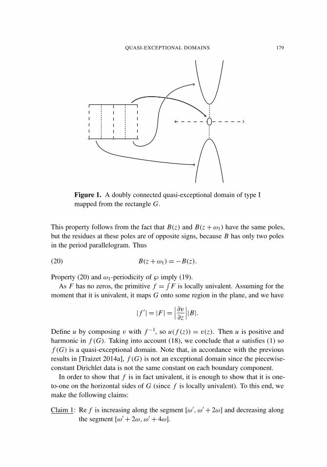
QUASI-EXCEPTIONAL DOMAINS 179
Figure 1. A doubly connected quasi-exceptional domain of type Imapped from the rectangle G.
This property follows from the fact that B(z) and B(z+ω1) have the same poles,but the residues at these poles are of opposite signs, because B has only two polesin the period parallelogram. Thus
(20) B(z+ω1)=−B(z).
Property (20) and ω1-periodicity of ℘ imply (19).As F has no zeros, the primitive f =
∫F is locally univalent. Assuming for the
moment that it is univalent, it maps G onto some region in the plane, and we have
| f ′| = |F | =∣∣∣∂v∂z
∣∣∣|B|.Define u by composing v with f −1, so u( f (z)) = v(z). Then u is positive andharmonic in f (G). Taking into account (18), we conclude that u satisfies (1) sof (G) is a quasi-exceptional domain. Note that, in accordance with the previousresults in [Traizet 2014a], f (G) is not an exceptional domain since the piecewise-constant Dirichlet data is not the same constant on each boundary component.
In order to show that f is in fact univalent, it is enough to show that it is one-to-one on the horizontal sides of G (since f is locally univalent). To this end, wemake the following claims:
Claim 1: Re f is increasing along the segment [ω′, ω′+ 2ω] and decreasing alongthe segment [ω′+ 2ω,ω′+ 4ω].

180 ALEXANDRE EREMENKO AND ERIK LUNDBERG
Claim 2: Im f < Im f (ω′) on the segment (ω′, ω′+ 2ω] and Im f > Im f (ω′) onthe segment [ω′+ 2ω,ω′+ 4ω).
Claim 3: Im f achieves its minimum and maximum on the segment [ω′, ω′+ 4ω]at ω′+ω and ω′+ 3ω, respectively.
Claim 4: Re f is increasing along the segment [0, 2ω] and Re f is decreasing alongthe segment [2ω, 4ω].
Claim 5: Im f attains its maximum on the segment [0, 2ω] at ω and its minimumon the segment [2ω, 4ω] at 3ω.
Claim 6: Im f (ω) < Im f (ω′+ω) < Im f (ω′+ 3ω) < Im f (3ω).
Claim 1 implies that Re f is monotone along each of the named segments, andsince Im f differs between the two segments by Claim 2, f must be one-to-oneon the top side of G. Claim 4 implies that f is one-to-one on each of the twosegments on the bottom side of G. Claims 3, 5, and 6 imply that the images ofthese three segments do not intersect each other. This shows that f is one-to-oneon the horizontal sides of G.
The claims can be established by the properties of f ′ = F = ∂zvB. First notethat, since v(z) is positive in G and vanishes on the horizontal sides of G, we have∂xv(z)= 0 on both sides, and for x ∈R we have ∂yv(x+ω3)< 0 and ∂yv(x)> 0. Inparticular, i∂zv(z)= i(∂xv− i∂yv)/2= ∂yv/2 is real. The function B(z) is a Jacobisn function, whose properties are well known [Akhiezer 1990, Section 47]. B(z)sends the top side of G to the unit circle, such that the four segments [ω′, ω′+ω],[ω′+ω,ω′+2ω], [ω′+2ω,ω′+3ω], and [ω′+3ω,ω′+4ω] correspond to the fourth,third, second, and first quadrants of the unit circle, respectively. Multiplicationby ∂zv(z) distorts this circle and rotates it by an angle of π/2 (since ∂zv(z)/ i ispositive), but preserves the two-fold symmetry. This determines the sign of the realand imaginary parts of f ′. Since dz = dx is purely real on the horizontal sidesof G, this gives the monotonicity of Re f stated in Claim 1. Claims 2 and 3 followfrom the sign of Im f ′ and the fact that Im f ′ is an odd function with respect toreflection in each of the points ω′+ω and ω′+ 3ω.
The four segments [0, ω], [ω, 2ω], [2ω, 3ω], and [3ω, 4ω] on the bottom sideof G are sent to the second, first, fourth, and third quadrants of the unit circle,respectively. Since ∂zv(z)/ i is negative along the bottom side of G, under f ′(z) thisbecomes the first, fourth, third, and second quadrants, respectively. This establishesClaim 4, and, combined with the reflectional symmetry, also Claim 5. Claim 6follows from the fact that ∂zv(z)B(z) > 0 along the vertical segment [ω,ω+ω′]and ∂zv(z)B(z) < 0 along [3ω, 3ω+ω′].

QUASI-EXCEPTIONAL DOMAINS 181
Figure 2. An example of type II with ω1 = 2, ω3 = 2 and ε = 0.5.
Figure 3. An example of type II with ω1 = 2, ω3 = 1.5, and ε = 0.4.
Remark. For the purpose of plotting Figure 1, instead of the above construction,we expressed F as a ratio of Weierstrass sigma functions:
f ′(z)= F(z)=σ(z−ω+ω′/2)2 · σ(z− 3ω+ω′/2)2
σ(z)2 · σ(z− 2ω) · σ(z− 6ω+ 2ω′),
where σ is a Weierstrass sigma function with fundamental “periods” 4ω, 2ω′ (butrecall that σ is not itself periodic). As usual, the shifts are chosen based on thezeros and poles of F , but one of the shifts must be replaced by an equivalent latticepoint in a different rectangle in order to satisfy [Akhiezer 1990, Section 14, (1)].This explains why one of the poles is placed at 6ω− 2ω′.
Example of type II. Only small modifications of the previous example are needed.Using the same G,G ′, ω1, ω3, we define h as the ω1-periodic function, positive andharmonic in G ′ except two logarithmic poles at iε and ω1+ iε, where ε ∈ (0, ω3/2).Then we can find constants c1 and c2 such that v = h+ c1 y+ c2 has critical pointsat ω1/2+ω3/2 and 3ω1/2+ω3/2.
Then vz is an elliptic function with periods ω1, 2ω3 with two simple poles at iεand −iε per period parallelogram. This elliptic function has the form
−i℘1+ c℘
+ ic0
for some small real c. The rest of the construction is the same as in the previousexample.
In a similar manner to the above, in order to plot Figures 2 and 3, we expressedF as a ratio of Weierstrass sigma functions:
f ′(z)= F(z)=σ(z−ω+ω′/2)2 · σ(z− 3ω+ω′/2)2
σ(z− iε) · σ(z+ iε) · σ(z− 2ω− iε) · σ(z− 6ω+ iε+ 2ω′).
Note that we have displayed the figures horizontally in order to plot two periods.

182 ALEXANDRE EREMENKO AND ERIK LUNDBERG
6. Hollow vortex equilibria
Let G j be smooth Jordan domains on the plane whose closures are disjoint, and
D = C \⋃
j
G j .
Let F be the complex potential of a flow of an ideal fluid which is divergence-freeand locally irrotational in D. If the pressure (determined by |F ′| according toBernoulli’s law) is constant on ∂D then G j can be interpreted as constant-pressuregas bubbles in the flow.
The first examples of this situation, with two bubbles, were constructed byPocklington [1895]. Periodic exceptional domains give periodic examples with onebubble per period, with the flow on the surface on the bubbles rotating in the samedirection [Baker et al. 1976] (see also [Crowdy and Green 2011]). Crowdy andGreen [2011] constructed periodic examples with two bubbles per period rotatingin the opposite direction. Our example of type II can be interpreted as a periodicflow with two bubbles per period rotating in the same direction.
The velocity at infinity in our examples is directed in the opposite directions onthe two sides of the row of bubbles.
Acknowledgments
We are grateful to Dmitry Khavinson for many helpful discussions and to RazvanTeodorescu for a crucial observation regarding the construction of the examplesof type I. We wish to thank Darren Crowdy for discussing with us the interestingconnection to the hollow vortex problem. We also thank the referee who mademany remarks which improved the paper.
References
[Akhiezer 1990] N. I. Akhiezer, Elements of the theory of elliptic functions, Translations of Mathe-matical Monographs 79, American Mathematical Society, Providence, RI, 1990. MR 91k:33016Zbl 0694.33001
[Baker et al. 1976] G. R. Baker, P. G. Saffman, and J. S. Sheffield, “Structure of a linear array ofhollow vortices of finite cross-section”, J. Fluid Mech. 74:3 (1976), 469–476. Zbl 0343.76004
[Brelot 1971] M. Brelot, On topologies and boundaries in potential theory, Lecture Notes in Mathe-matics 175, Springer, Berlin, 1971. MR 43 #7654 Zbl 0222.31014
[Carleman 1926] T. Carleman, “Extension d’un théorème de Liouville”, Acta Math. 48:3-4 (1926),363–366. MR 1555232 JFM 52.0316.02
[Crowdy and Green 2011] D. G. Crowdy and C. C. Green, “Analytical solutions for von Kármánstreets of hollow vortices”, Phys. Fluids 23:12 (2011), Article ID #126602.
[Gustafsson 1987] B. Gustafsson, “Application of half-order differentials on Riemann surfacesto quadrature identities for arc-length”, J. Analyse Math. 49 (1987), 54–89. MR 89b:30032Zbl 0652.30029

QUASI-EXCEPTIONAL DOMAINS 183
[Hauswirth et al. 2011] L. Hauswirth, F. Hélein, and F. Pacard, “On an overdetermined ellipticproblem”, Pacific J. Math. 250:2 (2011), 319–334. MR 2012g:58046 Zbl 1211.35207
[Heins 1950] M. Heins, “A lemma on positive harmonic functions”, Ann. of Math. (2) 52 (1950),568–573. MR 12,259b Zbl 0045.18803
[Khavinson et al. 2013] D. Khavinson, E. Lundberg, and R. Teodorescu, “An overdetermined problemin potential theory”, Pacific J. Math. 265:1 (2013), 85–111. MR 3095114 Zbl 1279.31003
[Kjellberg 1950] B. Kjellberg, “On the growth of minimal positive harmonic functions in a planeregion”, Ark. Mat. 1 (1950), 347–351. MR 12,410f Zbl 0040.05502
[Levin 1980] B. Y. Levin, Distribution of zeros of entire functions, Translations of MathematicalMonographs 5, American Mathematical Society, Providence, RI, 1980. Revised edition of 1964original. MR 81k:30011 Zbl 0152.06703
[Longuet-Higgins 1988] M. S. Longuet-Higgins, “Limiting forms for capillary-gravity waves”, J.Fluid Mech. 194 (1988), 351–375. MR 90f:76026 Zbl 0649.76005
[Pocklington 1895] H. C. Pocklington, “The configuration of a pair of equal and opposite hollowstraight vortices, of finite cross-section, moving steadily through fluid”, Proc. Camb. Philos. Soc. 8(1895), 178–187. JFM 25.1468.02
[Rashkovskii 2009] A. Rashkovskii, “Classical and new loglog-theorems”, Expo. Math. 27:4 (2009),271–287. MR 2010j:31001 Zbl 1177.31001
[Sakai 1981] M. Sakai, “Null quadrature domains”, J. Anal. Math. 40 (1981), 144–154. MR 84e:30069Zbl 0483.30002
[Traizet 2014a] M. Traizet, “Classification of the solutions to an overdetermined elliptic problem inthe plane”, Geom. Funct. Anal. 24:2 (2014), 690–720. MR 3192039 Zbl 1295.35344
[Traizet 2014b] M. Traizet, “Hollow vortices and minimal surfaces”, preprint, 2014. arXiv 1407.5308
Received June 4, 2014. Revised November 6, 2014.
ALEXANDRE EREMENKO
DEPARTMENT OF MATHEMATICS
PURDUE UNIVERSITY
150 N. UNIVERSITY STREET
WEST LAFAYETTE, IN 47907-2067UNITED STATES
ERIK LUNDBERG
DEPARTMENT OF MATHEMATICAL SCIENCES
FLORIDA ATLANTIC UNIVERSITY
777 GLADES ROAD
BOCA RATON, FL 33431UNITED STATES


PACIFIC JOURNAL OF MATHEMATICSVol. 276, No. 1, 2015
dx.doi.org/10.2140/pjm.2015.276.185
ENDOSCOPIC TRANSFER FOR UNITARY GROUPS ANDHOLOMORPHY OF ASAI L-FUNCTIONS
NEVEN GRBAC AND FREYDOON SHAHIDI
The analytic properties of the complete Asai L-functions attached to cusp-idal automorphic representations of the general linear group over a qua-dratic extension of a number field are obtained. The proof is based onthe comparison of the Langlands–Shahidi method and Mok’s endoscopicclassification of automorphic representations of quasisplit unitary groups.
Introduction 1851. The quasisplit unitary groups 1872. Eisenstein series and Asai L-functions 1893. Arthur parameters for unitary groups 1984. Holomorphy and nonvanishing of Asai L-functions 203Acknowledgements 208References 208
Introduction
In this paper we study the analytic properties of the complete Asai L-functionattached to a cuspidal automorphic representation of the general linear group overa quadratic extension of a number field. The approach is based on the Langlands–Shahidi method, combined with the knowledge of the poles of Eisenstein seriescoming from a recent endoscopic classification of automorphic representations ofthe quasisplit unitary groups by Mok [2015].
In order to state the main result more precisely, we introduce some notation. LetE/F be a quadratic extension of number fields, and let θ be the unique nontrivialelement in the Galois group Gal(E/F). Let AE and AF be the rings of adèles of Eand F , respectively. Let δ be any extension to A×E /E
× of the quadratic character ofA×F /F
× attached to E/F by class field theory.
Neven Grbac is supported in part by Croatian Science Foundation under the project 9364 and byUniversity of Rijeka research grant 13.14.1.2.02. Freydoon Shahidi is partially supported by NSFgrant DMS1162299.MSC2010: 11F66, 11F70, 11F72, 22E55.Keywords: Asai L-function, automorphic representation, endoscopic classification, spectral
decomposition, quasisplit unitary group.
185

186 NEVEN GRBAC AND FREYDOON SHAHIDI
For a cuspidal automorphic representation σ of GLn(AE), we denote by σ θ itsGalois conjugate and by σ its contragredient representation. We say that σ is Galoisself-dual if σ ∼= σ θ , that is, σ is isomorphic to its Galois conjugate contragredient.
Let L(s, σ, rA) denote the complete Asai L-function attached to σ and the Asairepresentation rA via the Langlands–Shahidi method. See Section 2.A for a definition.Our main result on the holomorphy and nonvanishing of the Asai L-functionL(s, σ, rA) is the following theorem.
Theorem 4.3. Let σ be a cuspidal automorphic representation of GLn(AE). LetL(s, σ, rA) (respectively, L(s, σ ⊗ δ, rA)) be the Asai (respectively, twisted Asai)L-function attached to σ , where δ is any extension to A×E /E
× of the quadraticcharacter of A×F /F
× attached to the extension E/F by class field theory.
(1) If σ is not Galois self-dual, i.e., if σ 6∼= σ θ , then L(s, σ, rA) is entire. It isnonzero for Re(s)≥ 1 and Re(s)≤ 0.
(2) If σ is Galois self-dual, i.e., if σ ∼= σ θ , then
(a) L(s, σ, rA) is entire, except for possible simple poles at s = 0 and s = 1,and nonzero for Re(s)≥ 1 and Re(s)≤ 0;
(b) exactly one of the L-functions L(s, σ, rA) and L(s, σ ⊗ δ, rA) has simplepoles at s = 0 and s = 1, while the other is holomorphic at those points.
The idea of the proof is to consider the Eisenstein series attached to σ on thequasisplit unitary group U2n(AF ) defined by the quadratic extension E/F , whereσ is viewed as a representation of the Levi factor of the Siegel maximal parabolicsubgroup of U2n in 2n variables. We look at the contribution of this Eisenstein seriesto the residual spectrum from two different points of view. On the one hand, by theLanglands–Shahidi method [2010], the poles of the Eisenstein series for the complexargument in the positive Weyl chamber are determined by certain ratio of the AsaiL-functions. The residues at such a pole span a residual representation of U2n(AF ).On the other hand, this residual representation should have an Arthur parameter,according to Mok’s endoscopic classification [2015] of automorphic representationsof quasisplit unitary groups (see also [Arthur 2005; 2013]). Comparing the possibleArthur parameters and poles of Asai L-functions, we are able to deduce the analyticproperties of these L-functions.
Mok’s work, as well as Arthur’s, still depends on the stabilization of the twistedtrace formula for the general linear group. Hence, our result is also conditionalon this stabilization. This issue is considered by Waldspurger [2014a; 2014b;2014c]. In our paper, we always make a remark when a partial result could havebeen obtained without using Mok’s work. In fact, the crucial insight coming fromendoscopic classification is holomorphy of the Asai L-function L(s, σ, rA) insidethe critical strip 0< Re(s) < 1.
ENDOSCOPIC TRANSFER AND HOLOMORPHY OF ASAI L -FUNCTIONS 187
This method was applied in [Grbac 2011] to the complete exterior and symmetricsquare L-functions attached to a cuspidal automorphic representation of GLn(AF ).It relies on Arthur’s endoscopic classification of automorphic representations forsplit classical groups [Arthur 2013; 2005]. The result and the approach are of thesame nature as the above theorem for Asai L-functions. The approach has alsoalready been used as a part of a long term project to study endoscopy via descentby Jiang, Liu and Zhang [Jiang et al. 2013].
A different approach to describing the analytic properties of L-functions is thatof integral representations. However, this approach usually gives holomorphy ofpartial L-functions, which is weaker than our result due to ramification or problemsat archimedean places. For the exterior square L-function this was pursued in [Bumpand Friedberg 1990; Kewat and Raghunathan 2012; Belt 2012], for the symmetricsquare L-function in [Bump and Ginzburg 1992] and more generally for twistedsymmetric square in a series of papers [Takeda 2014b; 2014a; 2013], and for theAsai L-functions in [Flicker 1988; Flicker and Zinoviev 1995; Anandavardhananand Rajan 2005].
The paper is organized as follows. In Section 1 we introduce the unitary groupstructure and fix the notation. In Section 2 the relation between poles of Eisensteinseries on quasisplit unitary groups and the Asai L-functions is investigated. Section 3provides a definition of Arthur parameters and packets for quasisplit unitary groupsin terms of results of Mok. Finally, in Section 4 we prove the main result on theanalytic properties of Asai L-functions.
1. The quasisplit unitary groups
1.A. Definition and basic structure. Let E/F be a quadratic extension of numberfields. The nontrivial Galois automorphism in the Galois group Gal(E/F) is denotedby θ . Let NE/F denote the norm map from E to F . Let AF and AE be the ringsof adèles of F and E , respectively, and A×F and A×E the corresponding groups ofidèles.
The quadratic character of A×F /F× attached to E/F by class field theory is
denoted by δE/F . We always identify δE/F with the corresponding character of theWeil group WF of F under class field theory. Let δ be any extension of δE/F to acharacter of A×E /E
×. Such extension is not unique.We denote by Fv the completion of F at the place v. If a place v of F does not
split in E , we always denote by w the unique place of E lying over v. Then Ew/Fvis a quadratic extension of local fields. If v splits in E , we denote by w1 and w2
the two places of E lying over v. Then we have Ew1∼= Ew2
∼= Fv. We use F∞ todenote the product of Fv over archimedean places.
For an integer N ≥ 2, we consider in this paper the F-quasisplit unitary groupUN in N variables defined by the extension E/F , viewed as an algebraic group

188 NEVEN GRBAC AND FREYDOON SHAHIDI
over F . More precisely, UN is a group scheme over F , whose functor of points isdefined as follows. Consider θ as an element of the Galois group Gal(F/F) trivialon F/E , where F is a fixed algebraic closure of F . Let V be an N -dimensionalvector space over E . We fix a form on V as in [Kim and Krishnamurthy 2004;2005], that is, let
Jn =
1. ..
1
and J ′N =
(0 Jn−Jn 0
)for N = 2n, 0 0 Jn
0 1 0−Jn 0 0
for N = 2n+ 1.
Then the functor of points of UN is given by
UN (R)= {g ∈ GLE⊗F R(V ⊗F R) : ∗g J ′N g = J ′N }
for any F-algebra R, where ∗g = tgθ is the conjugate transpose of g. In particular,the F-points of UN are given as
UN (F)= {g ∈ GLN (E) : ∗g J ′N g = J ′N }.
Writing N = 2n if N is even, and N = 2n+1 if N is odd, the F-rank of UN in bothcases equals n ≥ 1. For N = 1, the unitary group U1 in one variable is obtained byinserting N = 1 in the definition of UN . Its F-points are nothing else than
U1(F)= {x ∈ E× : θ(x)x = 1},
which is the norm-one subgroup E1 of E×.For m ≥ 1, let Gm = ResE/F GLm be the algebraic group over F obtained from
the general linear group GLm over E by restriction of scalars from E to F . If m ≤ n,it appears in the Levi factors of parabolic subgroups of UN .
We fix the Borel subgroup P0 of UN consisting of upper-triangular matrices.Let P0 = M0 N0, where M0 is a maximally split maximal torus of UN (i.e., onecontaining a maximal split torus of UN ; see [Shahidi 2010, Chapter I]), and N0 theunipotent radical of P0. Then
M0 ∼=
{G1× · · ·×G1 for N = 2n,G1× · · ·×G1×U1 for N = 2n+ 1,
with n copies of G1, so that the F-points of M0 are given by
M0(F)
=
{{diag(t1, . . . , tn, θ(tn)−1, . . . , θ(t1)−1) : ti ∈ E×} for N = 2n,{diag(t1, . . . , tn, t, θ(tn)−1, . . . , θ(t1)−1) : ti ∈ E×, t ∈ E1
} for N = 2n+1.

ENDOSCOPIC TRANSFER AND HOLOMORPHY OF ASAI L -FUNCTIONS 189
Let A0 be a maximal F-split torus of UN , which is a subtorus of M0. Then
A0(F)={{diag(t1, . . . , tn, t−1
n , . . . , t−11 ) : ti ∈ F×} for N = 2n,
{diag(t1, . . . , tn, 1, t−1n , . . . , t−1
1 ) : ti ∈ F×} for N = 2n+ 1.
The absolute root system8=8(UN ,M0) of UN with respect to M0 is of type AN−1.The root system 8red = 8(UN , A0) of UN with respect to A0 is a reduced rootsystem. It is of type Cn for N = 2n and of type BCn for N = 2n+ 1. We make thechoice of positive roots according to the fixed Borel subgroup P0, and let 1 be theset of simple roots. We order the simple roots as in Bourbaki [1968].
Let P be the Siegel maximal proper standard parabolic F-subgroup of UN . Thatis, it is defined, in a standard fashion, by a subset of simple roots obtained byremoving the last simple root in the Bourbaki ordering (cf. [Bourbaki 1968] and[Shahidi 2010, Section 1.2]). Let P = MP NP be the Levi decomposition of P ,where
MP ∼=
{Gn for N = 2n,Gn ×U1 for N = 2n+ 1,
is the Levi factor, and NP the unipotent radical.
1.B. L-groups. The L-group of UN is a semidirect product
LUN = GLN (C)o WF ,
where WF is the Weil group of F . It is acting on the connected component LU ◦N =GLN (C) through the quotient WF/WE ∼= Gal(E/F). The action of the nontrivialGalois automorphism θ ∈ Gal(E/F) is given by
θ(g)= J ′−1N
tg−1 J ′Nfor all g ∈ GLN (C).
The L-group of the Levi factor MP is a semidirect product
LMP =
{GLn(C)×GLn(C)o WF for N = 2n,GLn(C)×GL1(C)×GLn(C)o WF for N = 2n+ 1,
where the Weil group WF acts through the quotient WF/WE ∼= Gal(E/F) on theconnected component of the L-group, and θ ∈ Gal(E/F) acts by interchanging thetwo GLn(C) factors.
2. Eisenstein series and Asai L-functions
In this section we relate the analytic behavior of the Eisenstein series on the unitarygroup supported in the Siegel parabolic subgroup to a ratio of the Asai L-functionsappearing in its constant term. For the study of analytic properties of the Asai L-functions, it is sufficient to consider the even quasisplit unitary group U2n . However,

190 NEVEN GRBAC AND FREYDOON SHAHIDI
for completeness and future reference, we also study the Eisenstein series in theodd case.
We retain all the notation of Section 1. So, P is the Siegel maximal properstandard parabolic F-subgroup of UN , with the Levi factor MP ∼= Gn if N = 2nis even, and MP ∼= Gn ×U1 if N = 2n+ 1 is odd, and the unipotent radical NP .Recall that Gn = ResE/F GLn .
2.A. Asai L-functions. Let σ denote a cuspidal automorphic representation ofGn(AF )∼=GLn(AE) and ν a character of U1(AF )∼=A1
E trivial on U1(F)∼= E1. Tomake a convenient normalization in the case of odd unitary groups, as in [Rogawski1990] and [Goldberg 1994, Section 6], we denote by ν a unitary character ofGLn(AE) given by
ν(g)= ν(det(g ∗g−1))
for all g ∈ GLn(AE). Observe that det(g ∗g−1) is of norm one. Then we define acuspidal automorphic representation 6 of the Levi factor MP(AF ) as
6 =
{σ for N = 2n,(σ ν)⊗ ν for N = 2n+ 1.
More precisely, in the case of odd unitary groups the action of 6 is given by
6(g, t)= σ(g)ν(det(g ∗g−1))ν(t)
for g ∈ GLn(AE) and t ∈ A1E . We always assume that 6 is irreducible unitary and
trivial on AP(F∞)◦, the identity connected component of AP(F∞), where AP isa maximal F-split torus in the center of MP . The last condition is not restrictive.It is just a convenient normalization, obtained by twisting by a unitary character,which makes the poles of Eisenstein series real.
We define first the local L-functions. Let v be a place of F . By extension ofscalars from F to Fv, we may view the unitary group UN as an algebraic groupover Fv. This algebraic group is denoted by UN . Then we have the parabolicsubgroup Pv of UN defined over Fv with Levi decomposition MP,v NP,v, whereMP,v is the Levi factor and NP,v the unipotent radical.
In the case of the even unitary group, say N = 2n, the adjoint representation rv ofthe L-group LMP,v on the Lie algebra LnP,v of the L-group of NP,v is irreduciblefor all places v of F . If v does not split in E , then rv is called the Asai representation,as it generalizes the case considered by Asai in [1977]. We denote it by rA,v. Thissituation is labeled 2A2n−1− 2 in the list of [Shahidi 1988, Section 4] and [2010,Appendix C]. Explicit action of rA,v is given in [Goldberg 1994, Section 3].
In the case of the odd unitary group, say N = 2n + 1, the analogous adjointrepresentation is a direct sum r1,v⊕ r2,v of two irreducible representations for all

ENDOSCOPIC TRANSFER AND HOLOMORPHY OF ASAI L -FUNCTIONS 191
places v of F , ordered as in [Shahidi 1990]. If v does not split in E , then r2,v is thetwisted Asai representation rA,v⊗ δEw/Fv , where w is the unique place of E lyingover v. This situation is labeled 2A2n − 3 in the list of [1988, Section 4] and [2010,Appendix C].
For a cuspidal automorphic representation 6 of MP(AF ), let 6 ∼= ⊗′v6v be adecomposition into a restricted tensor product over all places. Let Rv be one ofthe adjoint representations defined above. Then the local L-functions L(s, 6v, Rv)attached to 6v and Rv are defined as follows.
• At archimedean places, they are the Artin L-functions attached to the Langlandsparameter of 6v as in [Shahidi 1985] (see also [2010, Section 8.2], and[Langlands 1989] where the Langlands parametrization over reals was firstintroduced).
• At unramified nonarchimedean places, they are given in terms of Satakeparameters of 6v (see [Shahidi 1988; 2010, Definition 2.3.5], and also [Harderet al. 1986] where Asai’s name came up first).
• At the remaining nonarchimedean places, they are defined using the Langlands–Shahidi method [Shahidi 1990, Section 7] (see also [Shahidi 2010, Sec-tion 8.4]).
The corresponding global L-functions are defined as the analytic continuationfrom the domain of convergence of the product over all places of local L-functionsL(s, 6v, Rv). According to [Langlands 1971] (see also [Shahidi 2010, Section 2.5]),the product over all places defining the global L-functions converges absolutely insome right half-plane Re(s) > C , where C is sufficiently large.
The global L-function obtained in this way from 6 = σ ∼=⊗′vσv and Rv = r1,vis denoted by L(s, σ, rA) and called the Asai L-function attached to σ . Its analyticproperties are the main concern of this paper.
The global L-function obtained from 6 ∼= ⊗′v6v and Rv = r2,v is denoted byL(s, 6, rA⊗ δE/F ) and called the twisted Asai L-function attached to 6. In fact, itis the same as the Asai L-function L(s, σ ⊗ δ, rA) attached to σ ⊗ δ (see [Goldberg1994]). Hence, the analytic properties of the twisted Asai L-function follow fromthe analytic properties of the Asai L-function attached to a twisted representation.Recall that δ is any extension of the quadratic character δE/F to A×E .
Finally, as shown in [Goldberg 1994], the choice of the normalization of 6 inthe case of odd unitary groups implies that the global L-function obtained from6 ∼=⊗′v6v and Rv = r1,v is the same as the principal L-function L(s, σ ) attachedto σ by [Godement and Jacquet 1972]. Its analytic properties are well known. It isentire, unless n = 1 and σ is the trivial character 1A×E
of A×E . In that case L(s, 1A×E)
is holomorphic except for simple poles at s = 0 and s = 1.
192 NEVEN GRBAC AND FREYDOON SHAHIDI
2.B. Eisenstein series. For s ∈ C and 6 a cuspidal automorphic representation ofMP(AF ) as above, let
I (s, 6)=
{IndUN (AF )
P(AF )(σ | det |sE) for N = 2n,
IndUN (AF )P(AF )
(σ ν| det |sE ⊗ ν) for N = 2n+ 1,
be the induced representation, where the induction is normalized. As in [Shahidi2010, page 108], we realize I (s, 6) for all s ∈ C on the same space W6 of smoothfunctions
f : NP(AF )MP(F)AP(F∞)◦\UN (AF )→ C,
K -finite with respect to a fixed maximal compact subgroup K of UN (AF ) compatibleto P (as in [Mœglin and Waldspurger 1995, Section I.1.4]), and such that the functionon MP(AF ) given by the assignment m 7→ f (mg) for m ∈ MP(AF ) belongs to thespace of 6 for all g ∈UN (AF ). The dependence on s ∈C is hidden in the action ofUN (AF ).
Given f ∈W6 and s ∈ C, set
fs(g)= f (g) exp〈s+ ρP, HP(g)〉
for all g ∈UN (AF ). Here ρP is the half-sum of positive roots not being the roots ofMP , and HP is a map
HP :UN (AF )→ Hom(X (MP)F ,R),
where X (MP)F denotes the group of F-rational characters of MP , defined onm = (mv)v ∈ MP(AF ) by the condition
exp〈χ, HP(m)〉 =∏v
|χ(mv)|v
for every χ ∈ X (MP)F , and extended via Iwasawa decomposition to UN (AF ) triv-ially on the unipotent radical NP(AF ) and the fixed maximal compact subgroup K(cf. [Shahidi 2010, Section 1.3]). Then the Eisenstein series is defined as the analyticcontinuation from the domain of convergence Re(s) > ρP of the series
E( f, s)(g)=∑
γ∈P(F)\UN (F)
f (γ g) exp〈s+ ρP, HP(γ g)〉 =∑
γ∈P(F)\UN (F)
fs(γ g)
for g ∈UN (AF ). The Eisenstein series E( f, s) has a finite number of simple polesin the real interval 0< s ≤ ρP, and all other poles have Re(s) < 0 (cf. [Mœglin andWaldspurger 1995, Section IV.1.11 and IV.3.12]). The residue of the Eisensteinseries E( f, s) at s > 0 is a square-integrable automorphic form on UN (AF ), butnot cuspidal, thus belonging to the residual spectrum of UN (AF ). In fact, suchresidues for all f ∈ W6 span the summand of the residual spectrum of UN (AF )
with cuspidal support in 6 (see [Mœglin and Waldspurger 1995, Section III.2.6]
ENDOSCOPIC TRANSFER AND HOLOMORPHY OF ASAI L -FUNCTIONS 193
or [Franke and Schwermer 1998, Section 1] for the decomposition of the space ofautomorphic forms with respect to their cuspidal support).
2.C. Asai L-functions in the constant term. Now we prove that the poles of Eisen-stein series E( f, s)(g) for Re(s) > 0 coincide with the poles for Re(s) > 0 of theratio of L-functions appearing in its constant term.
Theorem 2.1. Let σ be a cuspidal automorphic representation of Gn(AF ) ∼=
GLn(AE) and ν a unitary character of U1(AF ) ∼= A1E trivial on U1(F) ∼= E1.
As in Section 2.B, form a cuspidal automorphic representation 6 of the Levi factorMP(AF ) in UN . Then the poles with Re(s) > 0 of the Eisenstein series E( f, s) forsome f ∈W6 coincide with the poles satisfying Re(s) > 0 of
L(2s, σ, rA)
L(1+ 2s, σ, rA)if N = 2n,
L(s, σ )L(1+ s, σ )
·L(2s, σ ⊗ δ, rA)
L(1+ 2s, σ ⊗ δ, rA)if N = 2n+ 1,
where δ is any extension to A×E /E× of the quadratic character δE/F of A×F /F
×
attached to E/F by class field theory.
Remark 2.2. Observe the factor 2 appearing in the argument 2s of the Asai L-function in the case of even unitary groups. The reason is that we have chosen, asin [Shahidi 1992], the determinant character to normalize the identification withC of the complex parameter s in the Eisenstein series, instead of the character αgiven in terms of the half-sum of positive roots and the coroot of the unique simpleroot α not being a root of MP , as in [Shahidi 1990].
Proof of Theorem 2.1. This is an application of the Langlands spectral theory, usingthe Langlands–Shahidi method to normalize the intertwining operator.
The poles of the Eisenstein series E( f, s) coincide with the poles of its constantterm E( f, s)P along P . The constant term is defined as
E( f, s)P(g)=∫
NP (F)\NP (AF )
E( f, s)(ng) dn,
where dn is a fixed Haar measure on NP(AF ). On the other hand, the constant termcan be written as
E( f, s)P(g)= fs(g)+(M(s, 6,w0) f
)−s(g),
where M(s, 6,w0) is the standard intertwining operator. Here w0 is the uniquenontrivial Weyl group element such that w0(α) is a simple root for all simple roots αexcept the last one in the ordering of [Bourbaki 1968].
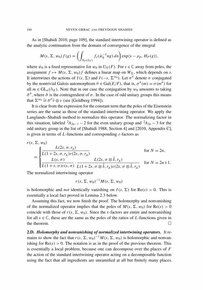
194 NEVEN GRBAC AND FREYDOON SHAHIDI
As in [Shahidi 2010, page 109], the standard intertwining operator is defined asthe analytic continuation from the domain of convergence of the integral
M(s, 6,w0) f (g)=(∫
NP (AF )
fs(w−10 ng) dn
)exp〈s− ρP, HP(g)〉,
where w0 is a fixed representative for w0 in UN (F). For s ∈C away from poles, theassignment f 7→ M(s, 6,w0) f defines a linear map on W6 , which depends on s.It intertwines the actions of I (s, 6) and I (−s, 6w0). Let σ θ denote σ conjugatedby the nontrivial Galois automorphism θ ∈ Gal(E/F), that is, σ θ (m)= σ(mθ ) forall m ∈ GLn(AE). Note that in our case the conjugation by w0 amounts to takingσ θ , where σ is the contragredient of σ . In the case of odd unitary groups this meansthat 6w0 ∼= σ θ ν⊗ ν (see [Goldberg 1994]).
It is clear from the expression for the constant term that the poles of the Eisensteinseries are the same as those of the standard intertwining operator. We apply theLanglands–Shahidi method to normalize this operator. The normalizing factor inthis situation, labeled 2A2n−1− 2 for the even unitary group and 2A2n − 3 for theodd unitary group in the list of [Shahidi 1988, Section 4] and [2010, Appendix C],is given in terms of L-functions and corresponding ε-factors as
r(s, 6,w0)
=
L(2s, σ, rA)
L(1+ 2s, σ, rA)ε(2s, σ, rA)for N = 2n,
L(s, σ )L(1+ s, σ )ε(s, σ )
·L(2s, σ ⊗ δ, rA)
L(1+ 2s, σ ⊗ δ, rA)ε(2s, σ ⊗ δ, rA)for N = 2n+1.
The normalized intertwining operator
r(s, 6,w0)−1 M(s, 6,w0)
is holomorphic and not identically vanishing on I (s, 6) for Re(s) > 0. This isessentially a local fact proved in Lemma 2.3 below.
Assuming this fact, we now finish the proof. The holomorphy and nonvanishingof the normalized operator implies that the poles of M(s, 6,w0) for Re(s) > 0coincide with those of r(s, 6,w0). Since the ε-factors are entire and nonvanishingfor all s ∈ C, these are the same as the poles of the ratios of L-functions given inthe theorem. �
2.D. Holomorphy and nonvanishing of normalized intertwining operators. It re-mains to show the fact that r(s, 6,w0)
−1 M(s, 6,w0) is holomorphic and nonvan-ishing for Re(s) > 0. The notation is as in the proof of the previous theorem. Thisis essentially a local problem, because one can decompose over the places of Fthe action of the standard intertwining operator acting on a decomposable functionusing the fact that all ingredients are unramified at all but finitely many places.
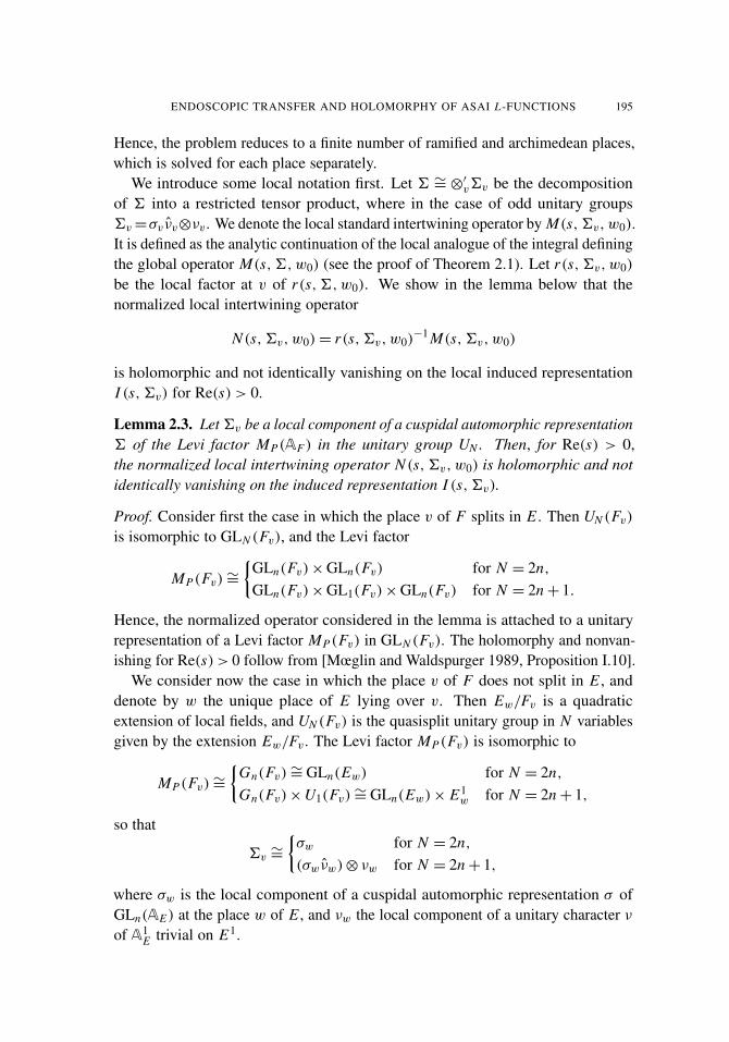
ENDOSCOPIC TRANSFER AND HOLOMORPHY OF ASAI L -FUNCTIONS 195
Hence, the problem reduces to a finite number of ramified and archimedean places,which is solved for each place separately.
We introduce some local notation first. Let 6 ∼= ⊗′v6v be the decompositionof 6 into a restricted tensor product, where in the case of odd unitary groups6v=σv νv⊗νv . We denote the local standard intertwining operator by M(s, 6v, w0).It is defined as the analytic continuation of the local analogue of the integral definingthe global operator M(s, 6,w0) (see the proof of Theorem 2.1). Let r(s, 6v, w0)
be the local factor at v of r(s, 6,w0). We show in the lemma below that thenormalized local intertwining operator
N (s, 6v, w0)= r(s, 6v, w0)−1 M(s, 6v, w0)
is holomorphic and not identically vanishing on the local induced representationI (s, 6v) for Re(s) > 0.
Lemma 2.3. Let6v be a local component of a cuspidal automorphic representation6 of the Levi factor MP(AF ) in the unitary group UN . Then, for Re(s) > 0,the normalized local intertwining operator N (s, 6v, w0) is holomorphic and notidentically vanishing on the induced representation I (s, 6v).
Proof. Consider first the case in which the place v of F splits in E . Then UN (Fv)is isomorphic to GLN (Fv), and the Levi factor
MP(Fv)∼={
GLn(Fv)×GLn(Fv) for N = 2n,GLn(Fv)×GL1(Fv)×GLn(Fv) for N = 2n+ 1.
Hence, the normalized operator considered in the lemma is attached to a unitaryrepresentation of a Levi factor MP(Fv) in GLN (Fv). The holomorphy and nonvan-ishing for Re(s) > 0 follow from [Mœglin and Waldspurger 1989, Proposition I.10].
We consider now the case in which the place v of F does not split in E , anddenote by w the unique place of E lying over v. Then Ew/Fv is a quadraticextension of local fields, and UN (Fv) is the quasisplit unitary group in N variablesgiven by the extension Ew/Fv. The Levi factor MP(Fv) is isomorphic to
MP(Fv)∼={
Gn(Fv)∼= GLn(Ew) for N = 2n,Gn(Fv)×U1(Fv)∼= GLn(Ew)× E1
w for N = 2n+ 1,
so that
6v ∼=
{σw for N = 2n,(σwνw)⊗ νw for N = 2n+ 1,
where σw is the local component of a cuspidal automorphic representation σ ofGLn(AE) at the place w of E , and νw the local component of a unitary character νof A1
E trivial on E1.
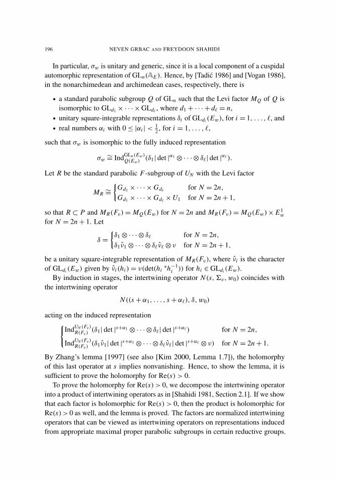
196 NEVEN GRBAC AND FREYDOON SHAHIDI
In particular, σw is unitary and generic, since it is a local component of a cuspidalautomorphic representation of GLn(AE). Hence, by [Tadic 1986] and [Vogan 1986],in the nonarchimedean and archimedean cases, respectively, there is
• a standard parabolic subgroup Q of GLn such that the Levi factor MQ of Q isisomorphic to GLd1 × · · ·×GLd` , where d1+ · · ·+ d` = n,
• unitary square-integrable representations δi of GLdi (Ew), for i = 1, . . . , `, and• real numbers αi with 0≤ |αi |<
12 , for i = 1, . . . , `,
such that σw is isomorphic to the fully induced representation
σw ∼= IndGLn(Ew)Q(Ew) (δ1| det |α1 ⊗ · · ·⊗ δ`| det |α`).
Let R be the standard parabolic F-subgroup of UN with the Levi factor
MR ∼=
{Gd1 × · · ·×Gd` for N = 2n,Gd1 × · · ·×Gd` ×U1 for N = 2n+ 1,
so that R ⊂ P and MR(Fv)= MQ(Ew) for N = 2n and MR(Fv)= MQ(Ew)× E1w
for N = 2n+ 1. Let
δ =
{δ1⊗ · · ·⊗ δ` for N = 2n,δ1ν1⊗ · · ·⊗ δ`ν`⊗ ν for N = 2n+ 1,
be a unitary square-integrable representation of MR(Fv), where νi is the characterof GLdi (Ew) given by νi (hi )= ν(det(hi
∗h−1i )) for hi ∈ GLdi (Ew).
By induction in stages, the intertwining operator N (s, 6v, w0) coincides withthe intertwining operator
N ((s+α1, . . . , s+α`), δ, w0)
acting on the induced representation{IndUN (Fv)
R(Fv) (δ1| det |s+α1 ⊗ · · ·⊗ δ`| det |s+α`) for N = 2n,
IndUN (Fv)R(Fv) (δ1ν1| det |s+α1 ⊗ · · ·⊗ δ`ν`| det |s+α` ⊗ ν) for N = 2n+ 1.
By Zhang’s lemma [1997] (see also [Kim 2000, Lemma 1.7]), the holomorphyof this last operator at s implies nonvanishing. Hence, to show the lemma, it issufficient to prove the holomorphy for Re(s) > 0.
To prove the holomorphy for Re(s) > 0, we decompose the intertwining operatorinto a product of intertwining operators as in [Shahidi 1981, Section 2.1]. If we showthat each factor is holomorphic for Re(s) > 0, then the product is holomorphic forRe(s)> 0 as well, and the lemma is proved. The factors are normalized intertwiningoperators that can be viewed as intertwining operators on representations inducedfrom appropriate maximal proper parabolic subgroups in certain reductive groups.

ENDOSCOPIC TRANSFER AND HOLOMORPHY OF ASAI L -FUNCTIONS 197
In our case these rank-one factors are normalized operators
N (2s+αi +α j , δi ⊗ δθj ),
for 1≤ i < j ≤ `, acting on the induced representations
IndGLdi+d j (Ew)Qi, j (Ew)
(δi | det |s+αi ⊗ δ θj | det |−s−α j
),
where Qi, j is the maximal standard proper parabolic subgroup of GLdi+d j with theLevi factor GLdi ×GLd j , and normalized operators{
N (s+αk, δk) for N = 2n,N (s+αk, (δk νk)⊗ ν) for N = 2n+ 1,
for 1≤ k ≤ `, acting on the induced representation{Ind
U2dk (Fv)Qk(Fv) (δk | det |s+αk ) for N = 2n,
IndU2dk+1(Fv)Qk(Fv) (δk νk | det |s+αk ⊗ ν) for N = 2n+ 1,
where Qk is the maximal standard proper parabolic subgroup of U2dk with the Levifactor Gdk if N = 2n, and of U2dk+1 with the Levi factor Gdk×U1 if N = 2n+1. Wesuppress the Weyl group element from the notation for these intertwining operators,because they are always determined by the maximal parabolic subgroup in question.
According to [Zhang 1997, Section 2], the rank-one normalized intertwiningoperator is holomorphic when the real part of its complex parameter is greater thanthe first negative point of reducibility of the induced representation on which it acts.For Re(s) > 0, using the bound on αi , we have
Re(s+αi +α j ) >−1 and Re(s+αk) >−12 .
But these two bounds are precisely the first negative points of reducibility in thecases Qi, j ⊂ GLdi+d j and Qk ⊂ U2dk or U2dk+1. This essentially follows fromthe standard module conjecture, proved in [Vogan 1978] for any quasisplit realgroup, and thus for complex groups as well, and in [Muic 2001] for quasisplitclassical groups over a p-adic field. In [Casselman and Shahidi 1998, Section 5]the reducibility points are determined in terms of local coefficients over any localfield. A convenient reference making explicit the first reducibility points of suchcomplementary series using local coefficients for any quasisplit classical group overa local field of characteristic zero is [Lapid et al. 2004, Lemma 2.6 and 2.7]. For thegeneral linear group the reducibility is obtained in [Zelevinsky 1980] over a p-adicfield, in [Speh 1981] over reals, and in [Wallach 1979] over complex numbers(see also [Kim 2000, Lemma 2.10]). For the unitary group over a nonarchimedeanfield, it is obtained in [Goldberg 1994, Section 3 and 6] by applying the generalreducibility result of [Shahidi 1990], while at an archimedean place, the L-functions

198 NEVEN GRBAC AND FREYDOON SHAHIDI
in the local coefficient that control reducibility are the L-functions of the restrictionto R× of a character of C× (see [Lapid et al. 2004, Lemma 2.6]). Thus, the rank-onefactors are all holomorphic and the lemma is proved. �
Remark 2.4. Kim and Krishnamurthy [2004; 2005] have proved the holomorphyand nonvanishing of normalized intertwining operators for a representation of theLevi factor of any maximal proper parabolic subgroup of UN , which is a localcomponent of a generic cuspidal automorphic representation. Since in our case allcuspidal automorphic representations of the Levi factor are generic, Lemma 2.3follows from their work. Their proof uses their stable base change lift and boundstowards the Ramanujan conjecture obtained by Luo, Rudnick and Sarnak [1999] tobound the exponents on the unitary group. In our case these bounds are not requiredbecause our unitary factor in the Levi is either trivial or rank zero. This simplifiesthe proof.
3. Arthur parameters for unitary groups
Our next task is to introduce the notion of Arthur parameters and the endoscopicclassification of automorphic representations for the quasisplit unitary group UN inN variables. We consider both the even and odd case for completeness, althoughfor the application to the analytic properties of the Asai L-functions only the evencase is required.
In [Mok 2015], the results of [Arthur 2013] (see also [Arthur 2005]) are extendedto the case of quasisplit unitary groups. As in [Arthur 2004], we avoid the conjecturalLanglands group by describing the parameters in terms of irreducible constituentsof the discrete spectrum of general linear groups. For quasisplit classical groupsthis approach was taken in [Mœglin 2008].
3.A. Arthur parameters. Let µ be a Galois self-dual cuspidal automorphic repre-sentation of GLm(AE). One of the crucial results in Mok’s proof of endoscopicclassification of representations in the discrete spectrum for quasisplit unitary groupsis the uniqueness (up to equivalence) of the twisted endoscopic datum associated toµ. This is the content of [Mok 2015, Theorem 2.4.2]. In fact, this unique endoscopicdatum is simple, thus, determining a unique sign κ ∈ {±1} attached to µ. Theparity of the endoscopic datum associated to µ is then defined as κ(−1)m−1 (as inSection 2.4 of the same reference). Using parity we make the following definitionas in [ibid., Theorem 2.5.4] (see also [Gan et al. 2012]).
Definition 3.1. Let µ be a Galois self-dual cuspidal automorphic representationof GLm(AE). We say that µ is Galois orthogonal (resp. Galois symplectic), if theparity of the unique twisted endoscopic datum associated to µ is +1 (resp. −1).

ENDOSCOPIC TRANSFER AND HOLOMORPHY OF ASAI L -FUNCTIONS 199
It turns out, as also proved by Mok, that this definition can be rephrased in termsof poles at s = 1 of the Asai L-function L(s, µ, rA) attached to µ.
Theorem 3.2 [Mok 2015, Theorem 2.5.4(a)]. Let µ be a Galois self-dual cuspidalautomorphic representation of GLm(AE). Thenµ is Galois orthogonal (resp. Galoissymplectic) if and only if the Asai L-function L(s, µ, rA) (resp. the twisted AsaiL-function L(s, µ⊗ δ, rA)) has a pole at s = 1, where δ is any extension to A×E /E
×
of the quadratic character δE/F of A×F /F× attached to E/F by class field theory.
We are now ready to define global Arthur parameters for the quasisplit unitarygroup UN in N variables. We in fact define the square-integrable Arthur parameters,which, according to [ibid., Theorem 2.5.2], parameterize global Arthur packetscontributing to the discrete automorphic spectrum of UN (AF ). These parametersdepend on the choice of certain character of A×E , trivial on E×, that defines anL-embedding of the L-group of UN into the L-group of G N (cf. [ibid., Section 2.1]).Roughly speaking, this character determines whether we view parameters as thestable or twisted base change of a representation in the discrete spectrum. Of course,the decomposition of the discrete spectrum is independent of that choice, and wetake it in this paper to be the trivial character of A×E , and suppress it from notation(see [ibid., Theorem 2.5.2]). The reason why Mok considers all possible charactersis that they are all required for the induction argument in the proof of endoscopicclassification.
Definition 3.3 (Arthur parameters). As before, let UN be the quasisplit unitarygroup in N variables given by a quadratic extension E/F of number fields. The set92(UN ) of square-integrable global Arthur parameters for UN is defined as the setof all unordered formal sums of formal tensor products of the form
ψ = (µ1 � ν(n1))� · · ·� (µ`� ν(n`)),
such that
(i) µi is a Galois self-dual cuspidal automorphic representation of GLmi (AE),that is, µi ∼= µ
θi ;
(ii) ni is a positive integer, and ν(ni ) is the unique ni -dimensional irreduciblealgebraic representation of SL2(C);
(iii) m1n1+ · · ·+m`n` = N ;
(iv) for i 6= j , we have µi 6∼=µ j or ni 6= n j , that is, the formal sum ψ is multiplicityfree;
(v) representation µi is Galois orthogonal (resp. Galois symplectic) if and only ifintegers ni and N are of the same parity (resp. different parity).
According to Theorem 3.2, condition (v) is equivalent to the condition
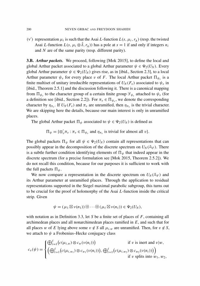
200 NEVEN GRBAC AND FREYDOON SHAHIDI
(v′) representationµi is such that the Asai L-function L(s, µi , rA) (resp. the twistedAsai L-function L(s, µi ⊗ δ, rA)) has a pole at s = 1 if and only if integers ni
and N are of the same parity (resp. different parity).
3.B. Arthur packets. We proceed, following [Mok 2015], to define the local andglobal Arthur packet associated to a global Arthur parameter ψ ∈92(UN ). Everyglobal Arthur parameter ψ ∈92(UN ) gives rise, as in [ibid., Section 2.3], to a localArthur parameter ψv for every place v of F . The local Arthur packet 5ψv is afinite multiset of unitary irreducible representations of UN (Fv) associated to ψv in[ibid., Theorem 2.5.1] and the discussion following it. There is a canonical mappingfrom 5ψv to the character group of a certain finite group Sψv attached to ψv (fora definition see [ibid., Section 2.2]). For πv ∈5ψv , we denote the correspondingcharacter by ηπv . If UN (Fv) and πv are unramified, then ηπv is the trivial character.We are skipping here the details, because our main interest is only in unramifiedplaces.
The global Arthur packet 5ψ associated to ψ ∈92(UN ) is defined as
5ψ = {⊗′
vπv : πv ∈5ψv and ηπv is trivial for almost all v}.
The global packets 5ψ for all ψ ∈ 92(UN ) contain all representations that canpossibly appear in the decomposition of the discrete spectrum on UN (AF ). Thereis a subtle further condition identifying elements of 5ψ that indeed appear in thediscrete spectrum (for a precise formulation see [Mok 2015, Theorem 2.5.2]). Wedo not recall this condition, because for our purposes it is sufficient to work withthe full packets 5ψ .
We now compare a representation in the discrete spectrum on UN (AF ) andits Arthur parameter at unramified places. Through the application to residualrepresentations supported in the Siegel maximal parabolic subgroup, this turns outto be crucial for the proof of holomorphy of the Asai L-function inside the criticalstrip. Given
ψ = (µ1 � ν(n1))� · · ·� (µ`� ν(n`)) ∈92(UN ),
with notation as in Definition 3.3, let S be a finite set of places of F , containing allarchimedean places and all nonarchimedean places ramified in E , and such that forall places w of E lying above some v 6∈ S all µi,w are unramified. Then, for v 6∈ S,we attach to ψ a Frobenius–Hecke conjugacy class
cv(ψ)=
⊕`
i=1(c(µi,w)⊗ cw(ν(ni ))
)if v is inert and v|w,(⊕`
i=1(c(µi,w1)⊗ cw1(ν(ni ))
),⊕`
i=1(c(µi,w2)⊗ cw2(ν(ni ))
))if v splits into w1, w2,

ENDOSCOPIC TRANSFER AND HOLOMORPHY OF ASAI L -FUNCTIONS 201
viewed as a semisimple conjugacy class in the L-group of G N over Fv, wherec(µi,w) ∈ GLmi (C) is the Satake parameter, and
cw(ν(ni ))= diag(q(ni−1)/2w , q(ni−3)/2
w , . . . , q−(ni−1)/2w
),
with qw the cardinality of the residue field of Ew. Observe that qw = q2v if v is inert
in E , and qw1 = qw2 = qv if v splits in E . The conjugacy classes cv(ψ) for v 6∈ Smay be viewed as the Satake parameters of the unramified constituents at places wof E lying above v of the induced representation
IndGLN (AE )R(AE )
(µ1| det |(n1−1)/2
⊗µ1| det |(n1−3)/2⊗ · · ·⊗µ1| det |−(n1−1)/2
⊗µ2| det |(n2−1)/2⊗µ2| det |(n2−3)/2
⊗ · · ·⊗µ2| det |−(n2−1)/2⊗ · · ·
⊗µ`| det |(n`−1)/2⊗µ`| det |(n`−3)/2
⊗ · · ·⊗µ`| det |−(n`−1)/2),
where R is the standard parabolic subgroup of GLN with the Levi factor GLm1 ×
· · · ×GLm1 ×GLm2 × · · · ×GLm2 × · · · ×GLm`× · · · ×GLm`
with ni copies ofGLmi in the product, and µi are unramified at v.
On the other hand, let π ∼=⊗′vπv be an irreducible automorphic representationappearing in the discrete spectrum on UN (AF ). Let S′ be a finite set of placesof F , containing all archimedean places, and such that for v 6∈ S′, we have thatUN (Fv) and πv are unramified. Then, for v 6∈ S′, the Satake isomorphism givesa Frobenius–Hecke conjugacy class c(πv) in the local L-group of UN over Fv.However, we may view c(πv) as a conjugacy class in the local L-group of G N
through the stable base change map of L-groups. This is consistent with our choiceof the trivial character in the definition of Arthur parameters.
According to the preliminary comparison of spectral sides of the trace formulasfor UN and the twisted trace formula for GLN , carried out in [Mok 2015, Sec-tion 4.3] (see also [Arthur 2013, Section 3.4]), for every irreducible automorphicrepresentation π of UN (AF ) appearing in the discrete spectrum, there is a uniquecorresponding parameter ψ ∈92(UN ) such that the Frobenius–Hecke conjugacyclasses cv(ψ) attached to ψ coincide at almost all places with the classes c(πv)attached to π . This observation is the key to the following proposition.
Remark 3.4. Strictly speaking the preliminary comparison of trace formulas givesunique ψ in a larger set of parameters 9(UN ) (see [Mok 2015] for a definition), butthe full proof of endoscopic classification shows that such ψ belongs to 92(UN ).
Proposition 3.5. Let P be the Siegel maximal proper parabolic F-subgroup of U2n .Let σ be a cuspidal automorphic representation of its Levi factor
MP(AF )∼= GLn(AE).

202 NEVEN GRBAC AND FREYDOON SHAHIDI
If the induced representation
IndU2n(AF )P(AF )
(σ ⊗ | det |sAE
)has a constituent in the discrete spectrum of U2n(AF ) for some s> 0, then its Arthurparameter is
ψ = σ � ν(2),
and in particular s = 12 and σ is Galois self-dual.
Proof. Since an automorphic representation is unramified at almost all places, thelocal component of an irreducible constituent π of the induced representation
IndU2n(AF )P(AF )
(σ ⊗ | det |sAE
)belonging to the discrete spectrum is the unramified representation with the Satakeparameter, viewed as a conjugacy class in the L-group of G2n as above,
c(πv)
=
{c(σw)⊗ diag(qs
w, q−sw ) if v is inert and v|w,(
c(σw1)⊗ diag(qsw1, q−sw1), c(σw2)⊗ diag(qs
w2, q−sw2))
if v splits into w1, w2,
for almost all places v of F . Recall that qw = q2v if v is inert, and qw1 = qw2 = qv
if v splits. We may also view c(πv) as the Satake parameter of the unramifiedconstituent of the local components at places w of E lying over v of the inducedrepresentation
IndGL2n(AE )Q(AE )
(σ | det |sAE
⊗ σ | det |−sAE
),
where Q is the standard parabolic subgroup of GL2n with the Levi factor GLn×GLn .By the observation made just before the statement of the proposition, these
Frobenius–Hecke conjugacy classes c(πv), viewed as conjugacy classes in the L-group of G2n , should match at almost all places the conjugacy classes cv(ψ) attachedto the Arthur parameter ψ ∈ 92(UN ) parameterizing π . As mentioned above,these cv(ψ) may be viewed as Satake parameters of the unramified constituent at vof certain induced representation of GL2n(AE). However, by the strong multiplicityone for general linear groups [Jacquet and Shalika 1981, Theorem 4.4], matchingof Satake parameters at almost all places for induced representations of GLN (AE)
implies that the inducing data for these representations are associate. Since Q isself associate, this means that the parabolic subgroup R determined by ψ as abovemust be Q, and thus that ψ is of the form
ψ = σ � ν(k),
where k = 2s+ 1. Since k = 2 by condition (iii) in Definition 3.3, it follows thats = 1
2 . As σ appears in ψ it is necessarily Galois self-dual. �
ENDOSCOPIC TRANSFER AND HOLOMORPHY OF ASAI L -FUNCTIONS 203
4. Holomorphy and nonvanishing of Asai L-functions
In this section we prove the analytic properties of the Asai L-functions as a conse-quence of Mok’s endoscopic classification [2015] of automorphic representationsof a quasisplit unitary group.
4.A. Analytic properties of Eisenstein series. The first task is to determine thepoles of Eisenstein series E( f, s) for Re(s) > 0. We now consider only the case ofeven quasisplit unitary group U2n .
Recall that for a cuspidal automorphic representation σ of GLn(AE), we let σ θ
denote σ conjugated by the nontrivial Galois automorphism θ ∈Gal(E/F). We saythat σ is Galois self-dual if it is isomorphic to σ θ , where σ is the contragredient of σ .
Theorem 4.1. Let σ be a cuspidal automorphic representation of the Levi factorMP(AF ) ∼= GLn(AE) in U2n . Then the Eisenstein series E( f, s) on U2n(AF ),constructed as in Section 2.B from functions f in the representation space Wσ onwhich induced representations I (s, σ ) are realized for all s, is
(1) holomorphic for Re(s)≥ 0, if σ is not Galois self-dual,
(2) holomorphic for Re(s)≥ 0, except for a possible simple pole at s = 12 , if σ is
Galois self-dual.
Proof. The Eisenstein series is holomorphic on the imaginary axis Re(s) = 0(see [Mœglin and Waldspurger 1995, Section IV.1.11]). Hence, we may assumeRe(s) > 0. Suppose that the Eisenstein series E( f, s) on U2n(AF ) has a poleat s = s0 > 0 for some f ∈ Wσ in the notation of Section 2. Since s0 > 0,the residues at s = s0 of E( f, s) when f ∈ Wσ span a residual automorphicrepresentation of U2n(AF ). But this residual representation is a constituent ofthe induced representation
IndU2n(AF )P(AF )
(σ ⊗ | det |s0
E
).
By Proposition 3.5, its Arthur parameter is
ψ = σ � ν(2),
where σ is Galois self-dual and s0 =12 . Therefore, the Eisenstein series E( f, s) is
holomorphic for Re(s) > 0, except for a possible pole at s = 12 if σ is Galois self-
dual, as claimed. The possible pole is simple, by the general theory of Eisensteinseries [Mœglin and Waldspurger 1995, Section IV.1.11] �
Remark 4.2. A significant part of Theorem 4.1 can be proved in a different way,without using Mok’s work on the Arthur classification for unitary groups [Mok2015], which is based on the trace formula, and still depends on the stabilization ofthe twisted trace formula for GLn .
204 NEVEN GRBAC AND FREYDOON SHAHIDI
For instance, if σ is not Galois self-dual, the following general argument providesholomorphy of the Eisenstein series for Re(s) > 0. By [Harish-Chandra 1968], seealso [Mœglin and Waldspurger 1995, Section IV.3.12], a necessary condition forthe Eisenstein series E( f, s) to have a pole for Re(s) > 0 and some f ∈Wσ is thatσw0 ∼= σ . But in our case, σw0 = σ θ , so that E( f, s) is holomorphic for Re(s) > 0and all f ∈Wσ if σ is not Galois self-dual.
If σ is Galois self-dual, there is a unitarity argument, which gives the analyticbehavior of the Eisenstein series for Re(s) ≥ 1
2 . However, the critical strip 0 <Re(s) < 1
2 remains out of reach. For completeness, we include this argument inSection 4.C below.
4.B. Analytic properties of Asai L-functions. The following theorem describescompletely the analytic properties of the Asai L-functions attached to a cuspidalautomorphic representation σ of GLn(AE). It is the main result of the paper.
Theorem 4.3. Let σ be a cuspidal automorphic representation of GLn(AE). LetL(s, σ, rA) (respectively, L(s, σ ⊗ δ, rA)) be the Asai (respectively, twisted Asai)L-function attached to σ , where δ is any extension to A×E /E
× of the quadraticcharacter of A×F /F
× attached to the extension E/F by class field theory.
(1) If σ is not Galois self-dual, that is, σ 6∼= σ θ , then L(s, σ, rA) is entire. It isnonzero for Re(s)≥ 1 and Re(s)≤ 0.
(2) If σ is Galois self-dual, that is, σ ∼= σ θ , then(a) L(s, σ, rA) is entire, except for possible simple poles at s = 0 and s = 1,
and nonzero for Re(s)≥ 1 and Re(s)≤ 0;(b) exactly one of the L-functions L(s, σ, rA) and L(s, σ ⊗ δ, rA) has simple
poles at s = 0 and s = 1, while the other is holomorphic at those points.
Proof. The idea of the proof goes back to [Shahidi 1981; 1988]. The proof ofholomorphy is based on Theorem 2.1, which relates the poles of Eisenstein seriesto the Asai L-functions, and Theorem 4.1 providing the analytic behavior of theEisenstein series. The nonvanishing, on the other hand, follows from consideringthe nonconstant term of the Eisenstein series as in [Shahidi 1981] (see also [Shahidi2010, Section 7]), and using Theorem 4.1 again. It is sufficient to prove the claimsfor Re(s)≥ 1
2 , due to the functional equation for Asai L-functions.We begin with the proof of holomorphy. Consider first the case of σ not Galois
self-dual. According to Theorem 4.1, the Eisenstein series attached to σ is holo-morphic for Re(s) > 0. Assume that L(s, σ, rA) has a pole for s = s0 > 0. Sincethe poles of E( f, s) for Re(s) > 0 coincide, according to Theorem 2.1, with thepoles of the ratio
(∗)L(2s, σ, rA)
L(1+ 2s, σ, rA),
ENDOSCOPIC TRANSFER AND HOLOMORPHY OF ASAI L -FUNCTIONS 205
the pole of the numerator at 2s = s0 > 0 should be canceled by a pole in thedenominator. Thus, L(z, σ, rA) should have a pole at z = s0 + 1. Repeating thisargument, we obtain a sequence of poles of the Asai L-function of the form s0+M ,where M is any nonnegative integer. This is a contradiction, because L(s, σ, rA) isholomorphic in the right half-plane of absolute convergence of the defining product.Thus, we proved that L(s, σ, rA) is entire.
Consider now the case of σ Galois self-dual. By Theorem 4.1, the Eisensteinseries E( f, s) attached to σ is holomorphic for Re(s) > 0, except for a possiblesimple pole at s = 1
2 . The same argument as in the previous case implies thatL(z, σ, rA) is holomorphic for Re(z) > 0, except for z = 1 if the Eisenstein serieshas a pole at s = 1
2 .To prove that a possible pole of L(z, σ, rA) at z = 1 is at most simple, we again
apply a similar argument. Suppose E( f, s) has a pole at s = 12 . It is simple by
Theorem 4.1. If L(z, σ, rA) had a higher order pole at z = 2s = 1, then Theorem 2.1would imply that there is a pole in the denominator of the ratio of Asai L-functionsin (∗). But this would mean that the Asai L-function has a pole at z+ 1= 2. TheEisenstein series is holomorphic at s = 1, so that the same argument as before givesa sequence of poles at all positive integers, which is a contradiction.
For nonvanishing, consider the nonconstant term E( f, s)ψ of the Eisensteinseries E( f, s) with respect to a fixed nontrivial additive character ψ of F\AF .According to [Shahidi 2010, Theorem 7.1.2], we have
E( f, s)ψ(e)=1
L S(1+ 2s, σ, rA)·
∏v∈S
Wv(ev),
where e and ev are the identity matrices, Wv is the ψv-Whittaker function attachedto f via a Jacquet integral, S is a finite set of places, containing all archimedeanplaces, outside which U2n(Fv), σv and ψv are all unramified, and L S(z, σ, rA) isthe partial Asai L-function attached to σ . As in [Shahidi 2010, Section 7.2], thereis a choice of f ∈ Wσ such that Wv(ev) 6= 0 for all v ∈ S. Thus, every zero ofL S(1+ 2s, σ, rA) for Re(s)≥ 0, equivalently Re(1+ 2s)≥ 1, would give a pole ofthe nonconstant term E( f, s)ψ . However, by Theorem 4.1, the Eisenstein seriesE( f, s), and thus E( f, s)ψ as well, is holomorphic for Re(s) ≥ 0, except for apossible pole at s = 1
2 , which may occur only if σ is Galois self-dual. Hence,L S(z, σ, rA) has no zeroes for Re(z)≥ 1, except possibly for z = 1. Since the localL-functions are nonvanishing, the same holds for the complete Asai L-functionL(z, σ, rA).
For σ Galois self-dual, the nonvanishing of L(z, σ, rA) at the remaining pointz = 1 follows from the identity
(∗∗) L(s, σ × σ θ )= L(s, σ, rA)L(s, σ, rA⊗ δE/F ),
206 NEVEN GRBAC AND FREYDOON SHAHIDI
where L(s, σ × σ θ ) is the Rankin–Selberg L-function, and recall that the twistedAsai L-function equals
L(s, σ, rA⊗ δE/F )= L(s, σ ⊗ δ, rA).
See [Goldberg 1994] for these identities. The poles of the Rankin–Selberg L-function L(s, σ × σ θ ) are known from [Jacquet and Shalika 1981]. For σ Galoisself-dual it has a simple pole at s = 1. Since σ ⊗ δ is Galois self-dual as well, wealready proved that both Asai L-functions on the right-hand side of (∗∗) have atmost a simple pole at s = 1. Hence, they are both nonzero at s = 1, and exactlyone of them has a simple pole at s = 1, as claimed. �
Remark 4.4. Once the holomorphy of the Asai and twisted Asai L-function isknown at some s0 with Re(s0) > 0, the argument using the Rankin–Selberg L-function at the end of this proof can be applied directly to obtain nonvanishing.However, the result of Jacquet and Shalika [1981] providing analytic properties ofthe Rankin–Selberg L-functions is very deep, and we preferred to give an argumentusing nonconstant term of the Eisenstein series whenever possible.
4.C. Holomorphy of Eisenstein series using a unitarity argument. We now givea different proof that the Eisenstein E( f, s), attached to a Galois self-dual cuspidalautomorphic representation σ of GLn(AF ) as above, is holomorphic for Re ≥ 1
2 ,except for a possible simple pole at s = 1
2 .It is sufficient to prove that E( f, s) is holomorphic for Re(s) > 1
2 . Indeed, sincewe always normalize σ to be trivial on AP(F∞)◦, the poles of the Eisenstein seriesare real. Hence, the only possible pole for Re(s)= 1
2 is at s = 12 . It is at most simple
pole, because all poles of Eisenstein series inside the closure of the positive Weylchamber are without multiplicity [Mœglin and Waldspurger 1995, Section IV.1.11].
Suppose that there is a simple pole of E( f, s) at s = s0 >12 . We follow an idea
of Kim [2000] based on the fact that residual representations are unitary. The spaceof residues of E( f, s) at s = s0 is a residual representation of U2n(AF ), which is aconstituent of the induced representation
I (s0, σ )= IndU2n(AF )P(AF )
(σ |det|s0
E
).
In particular, this residual representation is unitary, so that the induced representationshould have a unitary constituent. But then the local induced representation at everyplace v should have a unitary subquotient. Let v be a split nonarchimedean placeof F such that σv is unramified. The local induced representation at v is isomorphicto
I (s0, σv)∼= IndGL2n(Fv)P(Fv)
(σw1 |det|s0
Fv ⊗ σw2 |det|−s0Fv
),

ENDOSCOPIC TRANSFER AND HOLOMORPHY OF ASAI L -FUNCTIONS 207
where w1 and w2 are the two places of E lying above v. Since σw1 and σw2 areunramified unitary generic representations of GLn(Fv), according to [Tadic 1986],they are fully induced representations of the form
σw1∼=
IndGLn(Fv)Bn(Fv)
(µ1| |
α1 ⊗ · · ·⊗µk | |αk ⊗χ1⊗ · · ·⊗χl ⊗µk | |
−αk ⊗ · · ·⊗µ1| |−α1)
and
σw2∼=
IndGLn(Fv)Bn(Fv)
(µ′1| |
β1 ⊗ · · ·⊗µ′k′ | |βk′ ⊗χ ′1⊗ · · ·⊗χ
′
l ′ ⊗µ′
k′ | |−βk′ ⊗ · · ·⊗µ′1| |
−β1),
where Bn is a Borel subgroup of GLn , the exponents satisfy 0< αk < · · ·< α1 <12
and 0< βk′ < · · ·< β1 <12 , and µi , µ′i , χ j , χ ′j are unramified unitary characters of
F×v . Hence,
I (s0, σv)∼= IndGL2n(Fv)B2n(Fv)
(µ1| |
s0+α1 ⊗ · · ·⊗µk | |s0+αk ⊗χ1| |
s0 ⊗ · · ·⊗χl | |s0
⊗µk | |s0−αk ⊗ · · ·⊗µ1| |
s0−α1
⊗µ′1| |−s0+β1 ⊗ · · ·⊗µ′k′ | |
−s0+βk′ ⊗χ ′1| |−s0 ⊗ · · ·
⊗χ ′l ′ | |−s0 ⊗µ′k′ | |
−s0−βk′ ⊗ · · ·⊗µ′1| |−s0−β1
).
According to the description of the unitary dual of GL2n(Fv) [Tadic 1986], thisrepresentation would have a unitary subquotient, only if all the exponents whoseabsolute value is not smaller than 1
2 , induced with another character to a representa-tion of GL2(Fv), give a reducible representation with a unitary quotient of Spehtype. However, this is possible only if for every such exponent that is not less than12 in absolute value, there is another exponent such that their difference is exactly 1.
Having this in mind, consider the largest exponent in the above induced represen-tation. We write this exponent as s0+α1, and allow the possibility α1 = 0, whichhappens in the case k = 0 as there are no αi ’s. There should be another exponent ofthe form −s0±β, where β = β j for some j or β = 0, such that
(s0+α1)− (−s0±β)= 1.
But this implies2s0+α1∓β = 1,
which is possible for s0 >12 only if the sign of β is minus and α1 < β. As β is
certainly not greater than the largest of β j ’s, it follows that necessarily α1 < β1.However, considering the smallest exponent in the induced representation, that is,−s0−β1, where again β1 is set to zero if l = 0, we obtain the opposite inequality,β1<α1. This is a contradiction, proving that I (s0, σv) has not a unitary subquotient
208 NEVEN GRBAC AND FREYDOON SHAHIDI
for s0 >12 , and therefore, the Eisenstein series E( f, s) has no pole for Re(s) > 1
2 ,as claimed.
Acknowledgements
This paper was finalized during our visit to the Erwin Schrödinger Institute inVienna for the workshop Advances in the Theory of Automorphic Forms and theirL-Functions. We are grateful for the invitation and the ever stimulating atmosphereof the Erwin Schrödinger Institute. The first named author would like to thankGoran Muic for some useful discussions.
References
[Anandavardhanan and Rajan 2005] U. K. Anandavardhanan and C. S. Rajan, “Distinguished repre-sentations, base change, and reducibility for unitary groups”, Int. Math. Res. Not. 2005:14 (2005),841–854. MR 2006g:22013 Zbl 1070.22011
[Arthur 2004] J. Arthur, “Automorphic representations of GSp(4)”, pp. 65–81 in Contributions toautomorphic forms, geometry, and number theory (Baltimore, MD, 2002), edited by H. Hida et al.,Johns Hopkins University Press, Baltimore, MD, 2004. MR 2005d:11074 Zbl 1080.11037
[Arthur 2005] J. Arthur, “An introduction to the trace formula”, pp. 1–263 in Harmonic analysis, thetrace formula, and Shimura varieties, edited by J. Arthur et al., Clay Math. Proc. 4, Amer. Math.Soc., Providence, RI, 2005. MR 2007d:11058 Zbl 1152.11021
[Arthur 2013] J. Arthur, The endoscopic classification of representations: orthogonal and symplecticgroups, Amer. Math. Soc. Colloq. Publ. 61, Amer. Math. Soc., Providence, RI, 2013. MR 3135650Zbl 06231010
[Asai 1977] T. Asai, “On certain Dirichlet series associated with Hilbert modular forms and Rankin’smethod”, Math. Ann. 226:1 (1977), 81–94. MR 55 #2761 Zbl 0326.10024
[Belt 2012] D. D. Belt, On the holomorphy of exterior-square L-functions, thesis, Purdue Uni-versity, West Lafayette, IN, 2012, available at http://search.proquest.com/docview/1237150822.MR 3103748
[Bourbaki 1968] N. Bourbaki, Éléments de mathématique, Fasc. XXXIV: Groupes et algèbres deLie, Chapitre IV: Groupes de Coxeter et systèmes de Tits. Chapitre V: Groupes engendrés par desréflexions. Chapitre VI: Systèmes de racines, Actualités Scientifiques et Industrielles 1337, Hermann,Paris, 1968. Translated as Lie groups and Lie algebras: chapters 4–6, Springer, Berlin, 2002. MR 39#1590 Zbl 0186.33001
[Bump and Friedberg 1990] D. Bump and S. Friedberg, “The exterior square automorphic L-functionson GL(n)”, pp. 47–65 in Festschrift in honor of I. I. Piatetski-Shapiro on the occasion of his sixtiethbirthday, II: Papers in analysis, number theory and automorphic L-functions (Tel Aviv, 1989),edited by S. Gelbart et al., Israel Math. Conf. Proc. 3, Weizmann, Jerusalem, 1990. MR 93d:11050Zbl 0712.11030
[Bump and Ginzburg 1992] D. Bump and D. Ginzburg, “Symmetric square L-functions on GL(r)”,Ann. of Math. (2) 136:1 (1992), 137–205. MR 93i:11058 Zbl 0753.11021
[Casselman and Shahidi 1998] W. Casselman and F. Shahidi, “On irreducibility of standard modulesfor generic representations”, Ann. Sci. École Norm. Sup. (4) 31:4 (1998), 561–589. MR 99f:22028Zbl 0947.11022

ENDOSCOPIC TRANSFER AND HOLOMORPHY OF ASAI L -FUNCTIONS 209
[Flicker 1988] Y. Z. Flicker, “Twisted tensors and Euler products”, Bull. Soc. Math. France 116:3(1988), 295–313. MR 89m:11049 Zbl 0674.10026
[Flicker and Zinoviev 1995] Y. Z. Flicker and D. Zinoviev, “On poles of twisted tensor L-functions”,Proc. Japan Acad. Ser. A Math. Sci. 71:6 (1995), 114–116. MR 96f:11075 Zbl 0983.11023
[Franke and Schwermer 1998] J. Franke and J. Schwermer, “A decomposition of spaces of auto-morphic forms, and the Eisenstein cohomology of arithmetic groups”, Math. Ann. 311:4 (1998),765–790. MR 99k:11077 Zbl 0924.11042
[Gan et al. 2012] W. T. Gan, B. H. Gross, and D. Prasad, “Symplectic local root numbers, centralcritical L values, and restriction problems in the representation theory of classical groups”, pp. 1–109in Sur les conjectures de Gross et Prasad, vol. I, Astérisque 346, Société Mathématique de France,Paris, 2012. MR 3202556 Zbl 1280.22019 arXiv 0909.2999
[Godement and Jacquet 1972] R. Godement and H. Jacquet, Zeta functions of simple algebras,Lecture Notes in Math. 260, Springer, Berlin, 1972. MR 49 #7241 Zbl 0244.12011
[Goldberg 1994] D. Goldberg, “Some results on reducibility for unitary groups and local AsaiL-functions”, J. Reine Angew. Math. 448 (1994), 65–95. MR 95g:22031 Zbl 0815.11029
[Grbac 2011] N. Grbac, “On the residual spectrum of split classical groups supported in theSiegel maximal parabolic subgroup”, Monatsh. Math. 163:3 (2011), 301–314. MR 2012k:11063Zbl 1247.11080
[Harder et al. 1986] G. Harder, R. P. Langlands, and M. Rapoport, “Algebraische Zyklen auf Hilbert–Blumenthal-Flächen”, J. Reine Angew. Math. 366 (1986), 53–120. MR 87k:11066 Zbl 0575.14004
[Harish-Chandra 1968] Harish-Chandra, Automorphic forms on semisimple Lie groups, Lecture Notesin Math. 62, Springer, Berlin, 1968. MR 38 #1216 Zbl 0186.04702
[Jacquet and Shalika 1981] H. Jacquet and J. A. Shalika, “On Euler products and the classification ofautomorphic forms, II”, Amer. J. Math. 103:4 (1981), 777–815. MR 82m:10050b Zbl 0491.10020
[Jiang et al. 2013] D. Jiang, B. Liu, and L. Zhang, “Poles of certain residual Eisenstein series ofclassical groups”, Pacific J. Math. 264:1 (2013), 83–123. MR 3079762 Zbl 06203663
[Kewat and Raghunathan 2012] P. K. Kewat and R. Raghunathan, “On the local and global exteriorsquare L-functions of GLn”, Math. Res. Lett. 19:4 (2012), 785–804. MR 3008415 Zbl 06165853
[Kim 2000] H. H. Kim, “Langlands–Shahidi method and poles of automorphic L-functions, II”,Israel J. Math. 117 (2000), 261–284. MR 2001i:11059a Zbl 1041.11035
[Kim and Krishnamurthy 2004] H. H. Kim and M. Krishnamurthy, “Base change lift for odd unitarygroups”, pp. 116–125 in Functional analysis VIII (Dubrovnik, 2003), edited by D. Bakic et al.,Various Publ. Ser. (Aarhus) 47, Aarhus University, Aarhus, 2004. MR 2006a:11154 Zbl 1146.11313
[Kim and Krishnamurthy 2005] H. H. Kim and M. Krishnamurthy, “Stable base change lift fromunitary groups to GLn”, Int. Math. Res. Pap. 2005:1 (2005), 1–52. MR 2006d:22028 Zbl 1146.11314
[Langlands 1971] R. P. Langlands, Euler products (New Haven, CT, 1967), Yale MathematicalMonographs 1, Yale University Press, New Haven, CT, 1971. MR 54 #7387 Zbl 0231.20016
[Langlands 1989] R. P. Langlands, “On the classification of irreducible representations of realalgebraic groups”, pp. 101–170 in Representation theory and harmonic analysis on semisimple Liegroups, edited by P. J. Sally, Jr. and D. A. Vogan, Jr., Math. Surveys Monogr. 31, Amer. Math. Soc.,Providence, RI, 1989. MR 91e:22017 Zbl 0741.22009
[Lapid et al. 2004] E. Lapid, G. Muic, and M. Tadic, “On the generic unitary dual of quasisplit classicalgroups”, Int. Math. Res. Not. 2004:26 (2004), 1335–1354. MR 2005b:22021 Zbl 1079.22015
[Luo et al. 1999] W. Luo, Z. Rudnick, and P. Sarnak, “On the generalized Ramanujan conjecturefor GL(n)”, pp. 301–310 in Automorphic forms, automorphic representations, and arithmetic (Fort

210 NEVEN GRBAC AND FREYDOON SHAHIDI
Worth, TX, 1996), edited by R. S. Doran et al., Proc. Sympos. Pure Math. 66, Amer. Math. Soc.,Providence, RI, 1999. MR 2000e:11072 Zbl 0965.11023
[Mœglin 2008] C. Mœglin, “Formes automorphes de carré intégrable non cuspidales”, ManuscriptaMath. 127:4 (2008), 411–467. MR 2010i:11071 Zbl 05520091
[Mœglin and Waldspurger 1989] C. Mœglin and J.-L. Waldspurger, “Le spectre résiduel de GL(n)”,Ann. Sci. École Norm. Sup. (4) 22:4 (1989), 605–674. MR 91b:22028 Zbl 0696.10023
[Mœglin and Waldspurger 1995] C. Mœglin and J.-L. Waldspurger, Spectral decomposition andEisenstein series: a paraphrase of the Scriptures, Cambridge Tracts in Mathematics 113, CambridgeUniversity Press, 1995. MR 97d:11083 Zbl 0846.11032
[Mok 2015] C. P. Mok, “Endoscopic classification of representations of quasi-split unitary groups”,American Mathematical Society, Providence, RI, 2015. Mem. Amer. Math. Soc.
[Muic 2001] G. Muic, “A proof of Casselman–Shahidi’s conjecture for quasi-split classical groups”,Canad. Math. Bull. 44:3 (2001), 298–312. MR 2002f:22015 Zbl 0984.22007
[Rogawski 1990] J. D. Rogawski, Automorphic representations of unitary groups in three vari-ables, Annals of Mathematics Studies 123, Princeton University Press, 1990. MR 91k:22037Zbl 0724.11031
[Shahidi 1981] F. Shahidi, “On certain L-functions”, Amer. J. Math. 103:2 (1981), 297–355. MR 82i:10030 Zbl 0467.12013
[Shahidi 1985] F. Shahidi, “Local coefficients as Artin factors for real groups”, Duke Math. J. 52:4(1985), 973–1007. MR 87m:11049 Zbl 0674.10027
[Shahidi 1988] F. Shahidi, “On the Ramanujan conjecture and finiteness of poles for certain L-functions”, Ann. of Math. (2) 127:3 (1988), 547–584. MR 89h:11021 Zbl 0654.10029
[Shahidi 1990] F. Shahidi, “A proof of Langlands’ conjecture on Plancherel measures; complementaryseries for p-adic groups”, Ann. of Math. (2) 132:2 (1990), 273–330. MR 91m:11095 Zbl 0780.22005
[Shahidi 1992] F. Shahidi, “Twisted endoscopy and reducibility of induced representations for p-adicgroups”, Duke Math. J. 66:1 (1992), 1–41. MR 93b:22034 Zbl 0785.22022
[Shahidi 2010] F. Shahidi, Eisenstein series and automorphic L-functions, Amer. Math. Soc. Colloq.Publ. 58, Amer. Math. Soc., Providence, RI, 2010. MR 2012d:11119 Zbl 1215.11054
[Speh 1981] B. Speh, “The unitary dual of Gl(3, R) and Gl(4, R)”, Math. Ann. 258:2 (1981),113–133. MR 83i:22025 Zbl 0483.22005
[Tadic 1986] M. Tadic, “Classification of unitary representations in irreducible representations ofgeneral linear group (non-Archimedean case)”, Ann. Sci. École Norm. Sup. (4) 19:3 (1986), 335–382.MR 88b:22021 Zbl 0614.22005
[Takeda 2013] S. Takeda, “On a certain metaplectic Eisenstein series and the twisted symmetricsquare l-function”, preprint, University of Missouri, Columbia, MO, 2013, available at http://www.math.missouri.edu/~takedas/analytic_Eisen.pdf.
[Takeda 2014a] S. Takeda, “Metaplectic tensor products for automorphic representations of GL(r)”,preprint, 2014. arXiv 1303.2785
[Takeda 2014b] S. Takeda, “The twisted symmetric square L-function of GL(r)”, Duke Math. J. 163:1(2014), 175–266. MR 3161314 Zbl 06279927
[Vogan 1978] D. A. Vogan, Jr., “Gel’fand–Kirillov dimension for Harish-Chandra modules”, Invent.Math. 48:1 (1978), 75–98. MR 58 #22205 Zbl 0389.17002
[Vogan 1986] D. A. Vogan, Jr., “The unitary dual of GL(n) over an Archimedean field”, Invent. Math.83:3 (1986), 449–505. MR 87i:22042 Zbl 0598.22008

ENDOSCOPIC TRANSFER AND HOLOMORPHY OF ASAI L -FUNCTIONS 211
[Waldspurger 2014a] J.-L. Waldspurger, “Stabilisation de la formule des traces tordue, I: endoscopietordue sur un corps local”, preprint, Institut de Mathématiques de Jussieu, Paris, 2014, available athttp://webusers.imj-prg.fr/~jean-loup.waldspurger/stabilisationIfinal.pdf.
[Waldspurger 2014b] J.-L. Waldspurger, “Stabilisation de la formule des traces tordue, II: inté-grales orbitales et endoscopie sur un corps local non-archimédien; définitions et énoncés desrésultats”, preprint, Paris, 2014, available at http://webusers.imj-prg.fr/~jean-loup.waldspurger/stabilisationIIfinal.pdf.
[Waldspurger 2014c] J.-L. Waldspurger, “Stabilisation de la formule des traces tordue, III: intégralesorbitales et endoscopie sur un corps local non-archimédien; réductions et preuves”, preprint, Paris,2014, available at http://webusers.imj-prg.fr/~jean-loup.waldspurger/stabilisationIIIfinal.pdf.
[Wallach 1979] N. R. Wallach, “Representations of reductive Lie groups”, pp. 71–86 in Automorphicforms, representations and L-functions, 1 (Corvallis, OR, 1977), edited by A. Borel and W. Cas-selman, Proc. Sympos. Pure Math. 33, Amer. Math. Soc., Providence, RI, 1979. MR 80m:22024Zbl 0421.22006
[Zelevinsky 1980] A. V. Zelevinsky, “Induced representations of reductive p-adic groups, II: Onirreducible representations of GL(n)”, Ann. Sci. École Norm. Sup. (4) 13:2 (1980), 165–210.MR 83g:22012 Zbl 0441.22014
[Zhang 1997] Y. Zhang, “The holomorphy and nonvanishing of normalized local intertwining opera-tors”, Pacific J. Math. 180:2 (1997), 385–398. MR 98k:22076 Zbl 1073.22502
Received February 17, 2014. Revised April 17, 2014.
NEVEN GRBAC
DEPARTMENT OF MATHEMATICS
UNIVERSITY OF RIJEKA
RADMILE MATEJCIC 2HR-51000 RIJEKA
CROATIA
FREYDOON SHAHIDI
DEPARTMENT OF MATHEMATICS
PURDUE UNIVERSITY
150 N UNIVERSITY STREET
WEST LAFAYETTE, IN 47907-2067UNITED STATES

PACIFIC JOURNAL OF MATHEMATICSVol. 276, No. 1, 2015
dx.doi.org/10.2140/pjm.2015.276.213
QUASICONFORMAL HARMONIC MAPPINGS BETWEENDINI-SMOOTH JORDAN DOMAINS
DAVID KALAJ
Let D and � be Jordan domains with Dini-smooth boundaries. We provethat if f : D → � is a harmonic homeomorphism and f is quasiconfor-mal, then f is Lipschitz. This extends some recent results, where strongerassumptions on the boundary are imposed. Our result is optimal in that itcoincides with the best condition for Lipschitz behavior of conformal map-pings in the plane and conformal parametrizations of minimal surfaces.
1. Introduction and statement of the main result
Quasiconformal mappings. By definition, K-quasiconformal mappings (or qc map-pings for short) are orientation-preserving homeomorphisms f : D→� betweendomains D, �⊂ C that are contained in the Sobolev class W 1,2
loc (D) and for whichthe differential matrix and its determinant are coupled in the distortion inequality
(1-1) |Df (z)|2 ≤ K det Df (z) , where |Df (z)| = max|ξ |=1|Df (z)ξ |,
for some K ≥ 1. Here det Df (z) is the determinant of the formal derivative Df (z),which will be denoted in the sequel by J f (z). Note that condition (1-1) can bewritten in complex notation as
(1-2) (| fz| + | f z|)2≤ K (| fz|
2− | f 2
z |) a.e. on D,
or, what is the same,
| f z| ≤ k| fz| a.e. on D, where k = K−1K+1
, i.e., K = 1+k1−k
.
Harmonic mappings and the Hilbert transform. A mapping f is called harmonicin a region D if it has the form f = u+ iv, where u and v are real-valued harmonicfunctions in D. If D is simply connected, then there are two analytic functions hand g defined on D such that f has the representation
f = h+ g.
MSC2010: primary 30C55; secondary 31C05.Keywords: planar harmonic mappings, quasiconformal, Dini-smooth.
213

214 DAVID KALAJ
If f is a harmonic univalent function, then by Lewy’s theorem [1936], f has anonvanishing Jacobian and therefore is a diffeomorphism by the inverse mappingtheorem.
Let
P(r, x −ϕ)=1− r2
2π(1− 2r cos(x −ϕ)+ r2)
denote the Poisson kernel. If F ∈ L1(T), where T is the unit circle, we define thePoisson integral P[F] of F by
(1-3) P[F](z)=∫ 2π
0P(r, x −ϕ)F(ei x) dx, |z|< 1, z = reiϕ.
The function f (z)=P[F](z) is a harmonic mapping in the unit disk U={z : |z|<1},which belongs to the Hardy space h1(U). The mapping f is bounded in U if andonly if F ∈ L∞(T). Standard properties of the Poisson integral show that P[F]extends by continuity to F on U, provided that F is continuous. For these factsand standard properties of harmonic Hardy spaces, we refer to [Axler et al. 1992,Chapter 6; Duren 1970]. With the additional assumption that F is an orientation-preserving homeomorphism of this circle onto a convex Jordan curve γ , P[F] isan orientation-preserving diffeomorphism of the open unit disk onto the regionbounded by γ . This is indeed the celebrated theorem of Choquet–Radó–Kneser[Choquet 1945; Duren 2004]. This theorem is not true for nonconvex domains,but does hold under some additional assumptions. It has been extended in variousdirections (see for example [Jost 1981; Kalaj 2011b; Duren and Hengartner 1997]).
If f = u+ iv is a harmonic function defined in a Dini-smooth Jordan domainD then a harmonic function f = u+ i v is called the harmonic conjugate of f ifu+ i u and v+ i v are analytic functions. Notice that f is uniquely determined up toan additive constant. Let 8 : D→U be a conformal mapping, and let G ∈ L1(∂D).Then the Poisson integral of G with respect to the domain D is defined by
PD[G](z)=1
2π
∫∂D
1− |8(z)|2
|8(z)−8(ζ)|2G(ζ )|8′(ζ )| dζ.
Let χ be the boundary value of f and assume that χ is the boundary value of f .Then χ is called the Hilbert transform of χ and we also write it as H(χ). Assumethat χ ∈ L1(∂D). In particular, the Hilbert transform of a function χ ∈ L1(T) isdefined by the formula
(1-4) χ(τ )= H(χ)(τ )=−1π
∫ π
0+
χ(τ + t)−χ(τ − t)2 tan(t/2)
dt.
Here∫ π
0+ 8(t) dt := limε→0+∫ πε8(t) dt . This integral is improper and converges
for a.e. τ ∈ [0, 2π ]. This and other facts concerning the operator H used in this
QUASICONFORMAL AND HARMONIC MAPPINGS 215
paper can be found in [Zygmund 1959, Chapter VII]. Assume that χ, χ are inL1(T). Then
(1-5) P[χ ] = (P[χ ])∼,
where (k)∼ is the harmonic conjugate of k (see for instance [Pavlovic 2004, Theo-rem 6.1.3]).
If f = h + g : U→ � is a harmonic mapping then the radial and tangentialderivatives at z = rei t are defined by
∂r f (z)=1r(h′+ g′) and ∂t f (z)= i(h′− g′).
So r∂r f is the harmonic conjugate of ∂t f . We generalize this definition for amapping f = h+ g defined in a Jordan domain D. In order to do so, let 8= Rei2
be a conformal mapping of the domain D onto the unit disk. Then the radialderivative and tangent derivative of f in a point w ∈ D are defined by
∂R f (w)=1
|8(w)|D f (w)
(8(w)
8′(w)
)and ∂2 f (w)= D f (w)
(i8(w)
8′(w)
).
Here 8(w)/8′(w) and i(8(w)/8′(w)) are treated as two vectors from R2 ∼= C.Then it is easy to show that
R∂R f (w)=h′(w)8′(w)
+g′(w)
8′(w)and ∂2 f (w)= i
(h′(w)8′(w)
−g′(w)
8′(w)
).
This implies that R∂R f (w) and ∂2 f (w) are harmonic functions in D and R∂R f (w)is the harmonic conjugate of ∂2 f (w). Notice also that these derivatives are uniquelydetermined up to a conformal mapping 8. Assume further that D and � haveDini-smooth boundaries. If F : ∂D→ ∂� is the boundary function of f , and if∂2 f (w) is a bounded harmonic function, then
limw→w0
∂2 f (w)= F ′(w0),
where the limit is nontangential. Here
F ′(w0) :=∂(F ◦8−1)(ei t)
∂t,
where 8(w0) = ei t . If F ′ ∈ L1(∂D), then the harmonic function R∂R f (w) hasnontangential limits in almost every point of ∂D and its boundary value is theHilbert transform of F ′, namely
H(F ′)(w0)= limw→w0
R∂R f (w).

216 DAVID KALAJ
From now on the boundary value of f will be denoted by F . We will focuson orientation-preserving harmonic quasiconformal mappings between smoothdomains and investigate their Lipschitz character up to the boundary. For futurereference, we will say that a qc mapping f :U→� of the unit disk onto the Jordandomain � with rectifiable boundary is normalized if f (1) = w0, f (e2π i/3) = w1
and f (e4π i/3)= w2, where w0w1, w1w2 and w2w0 are arcs of γ = ∂� having thesame length |γ |/3.
Background. Let � be a Jordan domain with rectifiable boundary, and let γ be anarc-length parametrization of ∂�. We say that ∂� is C1 if γ ∈ C1. Then arg γ ′ iscontinuous and we let ω be its modulus of continuity. If ω satisfies
(1-6)∫ δ
0
ω(t)t
dt <∞, δ > 0,
we say that ∂� is Dini-smooth. Denote by C1,$ the class of all Dini-smoothJordan curves. The derivative of a conformal mapping f of the unit disk onto � iscontinuous and nonvanishing in D [Pommerenke 1975, Theorem 10.2] (see also[Warschawski 1961]). This implies that f is bi-Lipschitz continuous. For laterreference we refer to this result as Kellogg’s theorem, see [Kellogg 1912; Goluzin1969, p. 374]. Kellogg was the first to consider this type of result for C1,α domains,where 0 < α < 1. Warschawski [1970] proved the same result for a conformalparametrization of a minimal surface.
If f is merely quasiconformal and maps the unit disk onto itself, then Mori’stheorem implies that | f (z)− f (w)| ≤ M1(K )|z − w|1/K . The constant 1/K isthe best possible. If f is a conformal mapping of the unit disk onto a Jordandomain with a C1 boundary, then the function f is not necessarily Lipschitz (seefor example [Lesley and Warschawski 1978, p. 277]). This is why we need to addsome assumption, other than quasiconformality, as well as some smoothness of theimage curve that is better than C1 in order to obtain that the resulting mapping isLipschitz or bi-Lipschitz.
Since every conformal mapping in the plane is harmonic and quasiconformal, itis an interesting question to ask to what extent the smoothness of the boundary of aJordan domain � implies that a quasiconformal harmonic mapping of the unit diskonto � is Lipschitz. The first study of harmonic quasiconformal mappings of theunit disk onto itself was done by O. Martio [1968]. This paper has been generalizedin [Kalaj 2004] for qc mappings from the unit disk onto a convex Jordan domain.Pavlovic [2002] proved in a very interesting way that every qc harmonic mappingof the unit disk onto itself is Lipschitz. Kalaj [2008] proved that every qc harmonicmapping between two Jordan domains with C1,α boundary is Lipschitz. This resulthas its counterpart for non-Euclidean metrics [Kalaj and Mateljevic 2006]. For a

QUASICONFORMAL AND HARMONIC MAPPINGS 217
generalization of the last result to the several-dimensional case we refer to [Kalaj2013]. The problem of bi-Lipschitz continuity of a quasiconformal mapping of theunit disk onto a Jordan domain with C2 boundary has been solved in [Kalaj 2011a].The object of this paper is to extend some of these results.
New results. The following theorem is such an extension in which the Höldercontinuity is replaced by the more general Dini condition.
Theorem 1.1. Let f = P[F](z) be a harmonic normalized K-quasiconformalmapping between the unit disk and the Jordan domain� with γ = ∂�∈C1,$ . Thenthere exists a constant C ′ = C ′(γ, K ) such that
(1-7)∣∣∣∂F(eiϕ)
∂ϕ
∣∣∣≤ C ′ for almost every ϕ ∈ [0, 2π ],
and
(1-8) | f (z1)− f (z2)| ≤ K C ′|z1− z2| for z1, z2 ∈ U.
By using Theorem 1.1, we obtain the following improvement of [Kalaj 2008,Theorem 3.1].
Theorem 1.2. Let D and� be Jordan domains such that ∂D and ∂� are containedin C1,$ and let f : D 7→ � be a harmonic homeomorphism. The followingstatements hold true.
(a) If f is qc, then f is Lipschitz.
(b) If � is convex and f is qc, then f is bi-Lipschitz.
(c) If � is convex, then f is qc if and only log|F ′| and H(F ′) are in L∞(∂D).
Proof of Theorem 1.2. (a) Choose a conformal mapping 8 : U→ D so that the qcmapping f1 = f ◦8 is normalized. Then f1 is a qc harmonic mapping of the unitdisk onto � that satisfies the conditions of Theorem 1.1. This implies in particularthat f1 is Lipschitz. In view of Kellogg’s theorem, the mapping 8 is bi-Lipschitz.Thus f = f1 ◦8
−1 is Lipschitz.(b) If � is a convex domain, and if D = U, then by [Kalaj 2003], we have that
|D f (z)| ≥ 14 dist( f (0), ∂�)
for z ∈ U. If D is not the unit disk, then we make use of the conformal mapping8 : U→ D as in the proof of (a). Then we obtain
|D f (z)| = |D f1(z)|/|8′(z)| ≥ c.
Now by using the quasiconformality of f , we have that
|D f (z)|2 ≤ K J f (z).

218 DAVID KALAJ
Therefore
J f −1( f (z)) =1
J f (z)≤
Kc2 .
Since f −1 is K-quasiconformal, we have further that
|D f −1(w)|2 ≤ K J f −1(w)≤K 2
c2 .
This implies that f −1 is Lipschitz. This finishes the proof of (b).(c) If f is harmonic and quasiconformal, then by (b) it is bi-Lipschitz, and so its
boundary function F is bi-Lipschitz. Furthermore, R∂R f is a bounded harmonicfunction and this is equivalent with the fact that log |F ′| ∈ L∞(∂D). Since H(F ′)is its boundary function, it is bounded, i.e., it belongs to L∞(∂D).
We now prove the opposite implication. Since
∂2 f = PD[F ′] and R∂R f = PD[H(F ′)],
it follows that ∂2 f and R∂R f are bounded harmonic functions. This means that|D f | is bounded by a constant M . In order to show that f is quasiconformal, it isenough to show that the Jacobian of f is bigger than a positive constant in D. Letf1 = f ◦8−1, and let δ = dist( f1(0), ∂�) and κ =min |∂t f1(ei t)|. Then by [Kalaj2004, Corollary 2.9], we have
J f (8(w))|8′(w)|2 = J f1(w)≥
κδ
2.
SoJ f (z)≥ c > 0, z ∈ D.
We conclude that|D f (z)|2
J f (z)≤
M2
c. �
2. Preliminary results
Definition 2.1. Let ξ : [a, b] → C be a continuous function. The modulus ofcontinuity of ξ is
ω(t)= ωξ (t)= sup|x−y|≤t
|ξ(x)− ξ(y)|.
The function ξ is called Dini-continuous if
(2-1)∫ b−a
0
ωξ (t)t
dt <∞.
Let γ be a C1 Jordan curve γ with the length l=|γ | and assume that g : [0, l]→γ isits arc-length parametrization . We say that γ is Dini-smooth if g′ is Dini-continuous
QUASICONFORMAL AND HARMONIC MAPPINGS 219
on [0, l]. If ω(t) is the modulus of continuity of g′ for 0≤ t ≤ l, then we extend ωby ω(t)= ω(l) for t ≥ l.
A function F : T→ γ is called Dini-smooth if the function 8(t) = F(ei t) isDini-smooth, i.e.,
|8′(t)−8′(s)| ≤ ω(|t − s|),
where ω is Dini-continuous. Observe that every smooth C1,α Jordan curve isDini-smooth.
Let
(2-2) K(s, t)= Re [(g(t)− g(s)) · ig′(s)]
be a function defined on [0, l]× [0, l]. By K(s± l, t ± l)= K(s, t) we extend it toR×R. Suppose now that 9 : R 7→ γ is an arbitrary 2π -periodic Lipschitz functionsuch that 9|[0,2π) : [0, 2π) 7→ γ is an orientation-preserving bijective function.Then there exists an increasing continuous function ψ : [0, 2π ] 7→ [0, l] such that
(2-3) 9(τ)= g(ψ(τ)).
We have for a.e. eiτ∈ T that
9 ′(τ )= g′(ψ(τ)) ·ψ ′(τ ),
and therefore|9 ′(τ )| = |g′(ψ(τ))| · |ψ ′(τ )| = ψ ′(τ ).
Along with the function K we will also consider the function KF defined by
KF (t, τ )= Re [(9(t)−9(τ)) · i9 ′(τ )].
Here F(ei t)=9(t). It is easy to see that
(2-4) KF (t, τ )= ψ ′(τ )K(ψ(t), ψ(τ)).
Lemma 2.2. Let γ be a Dini-smooth Jordan curve and let g : [0, l] 7→ γ be anatural parametrization of a Jordan curve with g′ having modulus of continuity ω.Assume further that 9 : [0, 2π ] 7→ γ is an arbitrary parametrization of γ and letF(ei t)=9(t). Then
(2-5) |K(s, t)| ≤∫ min{|s−t |,l−|s−t |}
0ω(τ) dτ
and
(2-6) |KF (ϕ, x)| ≤ |ψ ′(ϕ)|∫ dγ (9(ϕ),9(x))
0ω(τ) dτ.
Here dγ (9(ϕ),9(x)) := min{|s(ϕ)− s(x)|, (l − |s(ϕ)− s(x)|)} is the (shortest)

220 DAVID KALAJ
distance between 9(ϕ) and 9(x) along γ , and it satisfies
|9(ϕ)−9(x)| ≤ dγ (9(ϕ),9(x))≤ Bγ |9(ϕ)−9(x)|.
Proof. Note that the estimate (2-5) has been proved in [Kalaj 2011b, Lemma 2.3].Now (2-6) follows from (2-5) and (2-4). �
A closed rectifiable Jordan curve γ satisfies a B-chord-arc condition for someconstant B > 1 if for all z1, z2 ∈ γ we have
(2-7) dγ (z1, z2)≤ B|z1− z2|.
Here dγ (z1, z2) is the length of the shorter arc of γ with endpoints z1 and z2. It isclear that if γ ∈ C1, then γ satisfies a chord-arc condition for some Bγ > 1. Thefollowing lemma is proved in [Kalaj 2012].
Lemma 2.3. Assume that γ satisfies a chord-arc condition for some B > 1. Thenfor every normalized K-qc mapping f between the unit disk U and the Jordandomain �= int γ we have
| f (z1)− f (z2)| ≤3γ (K )|z1− z2|α, z1, z2 ∈ T,
where
α =2
K (1+ 2B)2, 3γ (K )= 4 · 2α(1+ 2B)
√2πK |�|
log 2.
Next we recall some estimates for the Jacobian of a harmonic univalent function.
Lemma 2.4 [Kalaj 2011b, Lemma 3.1]. Suppose f =P[F] is a harmonic mappingsuch that F is a Lipschitz homeomorphism from the unit circle onto a Dini-smoothJordan curve γ . Let g be an arc-length parametrization of γ , letψ(t)=g−1(F(ei t)),and define 9(t)= F(ei t)= g(ψ(t)). Then for almost every τ ∈ [0, 2π ], the limit
J f (eiτ ) := limr→1
J f (reiτ )
exists and we have
(2-8) J f (eiτ )= ψ ′(τ )
∫ 2π
0
Re[(g(ψ(t))− g(ψ(τ))) · ig′(ψ(τ))
]2 sin2((t − τ)/2)
dt2π.
From Lemma 2.2 and Lemma 2.4 we obtain
Lemma 2.5. Under the conditions and notation of Lemma 2.4 we have
(2-9) J f (eiϕ)≤π
4|9 ′(ϕ)|
∫ π
−π
1x2
∫ dγ (F(ei(ϕ+x)),F(eiϕ))
0ω(τ) dτ dx
for a.e. eiϕ∈ T. Here ω is the modulus of continuity of g′.

QUASICONFORMAL AND HARMONIC MAPPINGS 221
Lemma 2.6. Let f = P[F](z) be a harmonic mapping between the unit disk U andthe Jordan domain �, with F ∈ C1,$ (T). Then the partial derivatives of f have acontinuous extension to the boundary of the unit disk.
Proof. In the proof of this lemma we denote ∂t9(ei t) by 9 ′(t). If F is Lipschitz-continuous, then 8=9 ′ ∈ L∞(T), and by the famous Marcel Riesz theorem (seefor example [Garnett 1981, Theorem 2.3]) there is a constant Ap such that
‖H(9 ′)‖L p(T) ≤ Ap‖9′‖L p(T)
for 1 < p < ∞. It follows that 8 = H(9 ′) ∈ L1. Since r fr is the harmonicconjugate of fτ , we have rwr = P[H(9 ′)] according to (1-5). By again usingFatou’s theorem, we have
(2-10) limr→1−
fr (reiτ )= H(9 ′)(τ ) a.e.
By (1-4), and by following the proof of Privaloff’s theorem [Zygmund 1959], weobtain that if |9 ′(x)−9 ′(y)| ≤ ω(|x − y|) for the Dini-continuous function, then
|H(9 ′)(x + h)− H(9 ′)(x)| ≤ A∫ 2h
0
ω(t)t
dt + Bh∫ 2π
h
ω(t)t2 dt +Cω(h),
for some absolute constants A, B and C . The detailed proof of the last fact can befound in [Garnett 1981, Theorem III 1.3.]. This implies that rwr (rei t) and ft(rei t)
have continuous extensions to the boundary and this is what we needed to prove. �
We now prove the following lemma needed in the sequel.
Lemma 2.7. Let A be a positive integrable function in [0, B] and assume thatq, Q > 0. Then there exists a continuous increasing function χ of (0,+∞) intoitself , depending on A, B, q and Q, such that the following hold: limx→∞ χ(x)=∞, the function g(x)= xχ(x) is convex, and∫ B
0A(x)χ(Qx−q) dx ≤ 4
∫ B
0A(x)dx .
Proof. First define inductively a sequence x0 = B, xk > 0 for k > 0, such thatxk+1 < xk/2, and∫ xk
0A(x) dx ≤ M2−k where M =
∫ B
0A(x)dx .
This is possible because A is integrable.Then define a continuous function ξ in [0, B] by ξ(xk)= k, and by extending it
linearly on each interval [xk+1, xk], that is
ξ(x)= k+xk − x
xk − xk+1, x ∈ [xk+1, xk].

222 DAVID KALAJ
It is easy to see that this function is convex, decreasing and tends to +∞ as x→∞.Moreover ∫ B
0A(x)ξ(x) dx ≤ M
∞∑k=0
(k+ 1)2−k= 4M.
Now set χ(x)= ξ((Q/x)τ ) for τ = 1/q . It remains to verify that xχ(x) is convex.This we do by differentiation:
(xχ(x))′ = ξ(Qτ x−τ )− Qτ τ x−τ ξ ′(Qτ x−τ ).
Since both summands are increasing, xχ(x) is convex. �
3. The proof of Theorem 1.1
By assumption of the theorem, the derivative of an arc-length parametrization g′
has a Dini-continuous modulus of continuity ω. We consider two cases.(i) F(ei t)=9(t) ∈C1,$ (T). Then by Lemma 2.6 the mapping f (z)=P[F](z)
is C1 up to the boundary. First we notice that for L = sup |9 ′(t)|, it is clear thatL <∞. We will prove more. We will show that L is bounded by a constant notdepending a priori on F . According to Lemma 2.6 and to (1-1), we have
(3-1) |D f (eiϕ)|2 = (| fz(eiϕ)| + | f z(eiϕ)|)2
= limz→eiϕ
(| fz(z)| + | f z(z)|)2
≤ K limz→eiϕ
(| fz(z)|2− | f z(z)|2)
= K (| fz(eiϕ)|2− | f z(eiϕ)|2)= K J f (eiϕ).
Furthermore, we have
(3-2) |D f (reiϕ)| = sup|ξ |=1|D f (reiϕ)ξ | ≥ |D f (reiϕ)(ieiϕ)| = |∂ϕ f (reiϕ)|.
This implies that
(3-3) |D f (eiϕ)|2 ≥ |∂ϕ f (eiϕ)|2 = |9 ′(ϕ)|2.
From (2-9), (3-3) and (3-1), we obtain:
|9 ′(ϕ)|2 ≤ K C1|9′(ϕ)|
∫ π
−π
1x2
∫ ρ(x,ϕ)
0ω(τ) dτ dx,
where
ρ(x, ϕ)= dγ(F(ei(ϕ+x)), F(eiϕ)
),

QUASICONFORMAL AND HARMONIC MAPPINGS 223
which is the same as
|9 ′(ϕ)| ≤ K C1
∫ π
−π
ρ(ϕ, x)x2
∫ 1
0ω(τρ(ϕ, x)) dτ dx .
Thus
|9 ′(ϕ)| ≤ K C1
∫ π
−π
ρ(ϕ, x)x2 ω(ρ(ϕ, x)) dx .
Let
(3-4) L := maxx∈[0,2π ]
|9 ′(x)| = maxx∈[0,2π ]
ψ ′(x)= ψ ′(ϕ).
Then
L ≤ K C1
∫ π
−π
ρ(ϕ, x)x2 ω(ρ(ϕ, x)) dx .
Furthermore, we have
M :=L
2πK C1≤
∫ π
−π
M(x, ϕ)dx2π,
where
M(x, ϕ)=ρ(ϕ, x)
x2 ω(ρ(ϕ, x)).
The idea is to make use of Lemma 2.7 with a convex function depending only onK to be found below.
Assume that χ : R+→ R+ is a continuous increasing function to be determinedin the sequel such that the function 8(t) = tχ(t) is convex. By using Jensen’sinequality to the previous integral with respect to the convex function 8, we obtain
8(M)≤∫ π
−π
8(M(x, ϕ))dx2π,
or equivalently,
(3-5) Mχ(M)≤∫ π
−π
M(x, ϕ)χ(M(x, ϕ))dx2π.
From (2-7) and (3-4) we deduce that
(3-6) ρ(ϕ, x)≤ Bγ L|x |.
On the other hand, since f is a normalized qc mapping, we have by Lemma 2.3that
(3-7) ρ(ϕ, x)≤ Bγ3γ (K )|x |α.

224 DAVID KALAJ
Notice that this time we used the boundary normalization. This implies that
(3-8) M(x, ϕ)=ρ(ϕ, x)
x2 ω(ρ(ϕ, x))≤Bγ L
xω(Bγ3γ (K )|x |α),
and
(3-9) M(x, ϕ)=ρ(ϕ, x)
x2 ω(ρ(ϕ, x))≤Bγ3γ (K )
x2−α ω(Bγ3γ (K )|x |α).
So, in view of Definition 2.1 we have
(3-10) M(x, ϕ)≤Bγ3γ (K )
x2−α ω(|γ |).
From (3-5) and (3-8), we obtain
(3-11) χ(
L2πK C1
)≤
∫ π
−π
K C1 Bγx
ω(Bγ3γ (K )|x |α)χ(
Bγ3γ (K )ω(|γ |)|x |2−α
)dx
= 2∫ π
0
K C1 Bγx
ω(Bγ3γ (K )|x |α)χ(
Bγ3γ (K )ω(|γ |)|x |2−α
)dx
=2K C1 Bγ
Bγ3γ (K )α
∫ B
0
ω(y)yχ(Qy1−2/α) dy,
whereB = Bγ3γ (K )πα and Q = ω(|γ |)(Bγ3γ (K ))2−2/α.
In view of the last term of (3-11), now is the time to determine the function χ .Lemma 2.7 with q = 2/α− 1 and A(y)= ω(y)/y, provides us with a function χsuch that 8 is convex and such that the estimate∫ B
0
ω(y)yχ(Qy1−2/α)dy ≤ 4
∫ B
0
ω(y)y
dy
holds. From (3-11), we have
χ( L
2πK C1
)≤
8K C1 BγBγ3γ (K )α
∫ B
0
ω(y)y
dy =: ϒ(K , �).
Since χ is increasing, we infer finally that
(3-12) L ≤ 2πK C1 ·χ−1(ϒ(K , �))=
π2
2K ·χ−1(ϒ(K , �)).
By the maximum principle, for z = reiϕ , we further have
|∂ϕ f (z)| ≤ L .
Since f is K-quasiconformal, we have
|Dw(z)| ≤ K |∂ϕ f (z)|.

QUASICONFORMAL AND HARMONIC MAPPINGS 225
This and the mean value inequality imply that
(3-13) | f (z)− f (z′)| ≤ K L|z− z′|, |z|< 1, |z′|< 1.
(ii) F /∈ C1,$ (T). In order to deal with nonsmooth F , we make use of anapproximation argument. We begin by this definition.
Definition 3.1. Let G be a domain in C and let a ∈ ∂G. We will say that Ga ⊂ Gis a neighborhood of a if there exists a disk D(a, r) := {z : |z− a|< r} such that(D(a, r)∩G)⊂ Ga .
Let t = ei x∈T. Then F(t)=9(x)∈ ∂�. Let g be an arc-length parametrization
of ∂� with g(ψ(x))= F(ei x), where ψ : [0, 2π ]→ [0, |γ |] is as in the first part ofthe proof. Put s =ψ(x). Since the modulus of continuity of g′ is a Dini-continuousfunction ω, there exists a neighborhood �t of 9(t) such that the derivative of itsarc-length parametrization g′t has modulus of continuity Ct ·ω. Moreover, thereexist positive numbers rt and Rt such that
�τt :=�t + ig′(s) · τ ⊂�, τ ∈ (0, Rt),(3-14)
∂�τt ⊂�, τ ∈ (0, Rt),(3-15)
g[s− rt , s+ rt ] ⊂ ∂�t .(3-16)
An example of a family �τt such that ∂�τt ∈C1,α for 0<α< 1 with property (3-14)has been given in [Kalaj 2008]. The same construction yields the family ∂�τt withthe above mentioned properties.
Take Uτ = f −1(�τt ). Let ητt be a conformal mapping of the unit disk onto Uτ
with normalized boundary condition: ητt (ei2kπ/3)= f −1(ζk) for k = 0, 1, 2, where
ζ0, ζ1, ζ2 are three points of ∂�τt of equal distance. Then the mapping
f τt (z) := f (ητt (z))− ig′(s) · τ
is a harmonic K-quasiconformal mapping of the unit disk onto �t satisfying theboundary normalization. Moreover,
f τt = P[Fτt ] ∈ C1(U)
for some function Fτt ∈ C1(T).Since [0, l] is compact, there exists a finite family of Jordan arcs
γ j = g(s j − rs j /2, s j + rs j /2), j = 1, . . . , n,
covering γ . Assume that F(t j )= s j . Let
F j,τ := Fτt j, a j,τ := η
τt j
and f j,τ := f τt j.
226 DAVID KALAJ
Using the case F ∈ C1,$ , it follows that there exists a constant C ′j = C ′(K , γ j )
such that|∂ϕF ′j,τ (e
iϕ)| ≤ C ′jand
(3-17) | f j,τ (z1)− f j,τ (z2)| ≤ K C ′j |z1− z2|.
Since a j,τ (z) converges uniformly on compact subsets of U to the function a j,0(z)when τ → 0, and since f j,τ = f ◦ a j,τ , inequality (3-17) implies
(3-18) | f j (z1)− f j (z2)| ≤ K C ′j |z1− z2| for z1, z2 ∈ U,
where f j = f ◦ a j,0 = P[F j ]. For z1 = ei t and z2 = eiϕ for t→ ϕ, we obtain that|∂ϕF j (eiϕ)| ≤ K C ′j a.e. Since the mapping b j = a−1
0, j can be extended conformallyacross the arc S j = f −1(λ j ), where λ j = g(s j− ts j , s j+ ts j ), there exists a constantL j such that |b j (z)|≤ L j on S′j =T∩ f −1(γ j ) for j=1, . . . , n. Hence |∂ϕF(eiϕ)|≤
K C ′j · L j on S′j . Let C ′ = max{K C ′j · L j : j = 1, . . . , n}. Inequalities (1-7) and(1-8) easily follow from T =
⋃nj=1 S′j .
Notice that we can now repeat the first part of the proof for a Lipschitz f =P[F]in order to obtain a more concrete Lipschitz constant, i.e., the constant L satisfying(3-12). The proof is complete.
Acknowledgement
I am grateful to professor Alexandre Eremenko, whose idea is used in the proofof Lemma 2.7, for his numerous useful suggestions and corrections that havesubstantially improved this paper. I am grateful to the anonymous referee for someuseful suggestions and corrections.
References
[Axler et al. 1992] S. Axler, P. Bourdon, and W. Ramey, Harmonic function theory, Graduate Textsin Mathematics 137, Springer, New York, 1992. MR 93f:31001 Zbl 0765.31001
[Choquet 1945] G. Choquet, “Sur un type de transformation analytique généralisant la représentationconforme et définie au moyen de fonctions harmoniques”, Bull. Sci. Math. (2) 69 (1945), 156–165.MR 8,93a Zbl 0063.00851
[Duren 1970] P. L. Duren, Theory of H p spaces, Pure and Applied Mathematics 38, Academic Press,New York, 1970. MR 42 #3552 Zbl 0215.20203
[Duren 2004] P. Duren, Harmonic mappings in the plane, Cambridge Tracts in Mathematics 156,Cambridge Univ. Press, 2004. MR 2005d:31001 Zbl 1055.31001
[Duren and Hengartner 1997] P. Duren and W. Hengartner, “Harmonic mappings of multiply con-nected domains”, Pacific J. Math. 180:2 (1997), 201–220. MR 99f:30051 Zbl 0885.30020
[Garnett 1981] J. B. Garnett, Bounded analytic functions, Pure and Applied Mathematics 96, Aca-demic Press, New York, 1981. MR 83g:30037 Zbl 0469.30024

QUASICONFORMAL AND HARMONIC MAPPINGS 227
[Goluzin 1969] G. M. Goluzin, Geometric theory of functions of a complex variable, Transla-tions of Mathematical Monographs 26, Amer. Math. Soc., Providence, RI, 1969. MR 40 #308Zbl 0183.07502
[Jost 1981] J. Jost, “Univalency of harmonic mappings between surfaces”, J. Reine Angew. Math. 324(1981), 141–153. MR 82h:58013 Zbl 0453.53036
[Kalaj 2003] D. Kalaj, “On harmonic diffeomorphisms of the unit disc onto a convex domain”,Complex Var. Theory Appl. 48:2 (2003), 175–187. MR 2003m:30043 Zbl 1041.30006
[Kalaj 2004] D. Kalaj, “Quasiconformal harmonic functions between convex domains”, Publ. Inst.Math. (Beograd) (N.S.) 76:90 (2004), 3–20. MR 2005j:30032 Zbl 1220.30032
[Kalaj 2008] D. Kalaj, “Quasiconformal and harmonic mappings between Jordan domains”, Math. Z.260:2 (2008), 237–252. MR 2009e:30038 Zbl 1151.30014
[Kalaj 2011a] D. Kalaj, “Harmonic mappings and distance function”, Ann. Sc. Norm. Super. Pisa Cl.Sci. (5) 10:3 (2011), 669–681. MR 2012j:30054 Zbl 1252.30018
[Kalaj 2011b] D. Kalaj, “Invertible harmonic mappings beyond the Kneser theorem and quasiconfor-mal harmonic mappings”, Studia Math. 207:2 (2011), 117–136. MR 2012k:30065 Zbl 1279.30032
[Kalaj 2012] D. Kalaj, “On boundary correspondences under quasiconformal harmonic mappings be-tween smooth Jordan domains”, Math. Nach. 285:2-3 (2012), 283–294. MR 2881282 Zbl 1251.30032
[Kalaj 2013] D. Kalaj, “A priori estimate of gradient of a solution of a certain differential inequalityand quasiconformal mappings”, J. Anal. Math. 119:1 (2013), 63–88. MR 3043147 Zbl 1270.35148
[Kalaj and Mateljevic 2006] D. Kalaj and M. Mateljevic, “Inner estimate and quasiconformal har-monic maps between smooth domains”, J. Anal. Math. 100 (2006), 117–132. MR 2008b:30033Zbl 1173.30311
[Kellogg 1912] O. D. Kellogg, “Harmonic functions and Green’s integral”, Trans. Amer. Math. Soc.13:1 (1912), 109–132. MR 1500909 JFM 43.0889.01
[Lesley and Warschawski 1978] F. D. Lesley and S. E. Warschawski, “On conformal mappings withderivative in VMOA”, Math. Z. 158:3 (1978), 275–283. MR 57 #6393 Zbl 0374.30007
[Lewy 1936] H. Lewy, “On the non-vanishing of the Jacobian in certain one-to-one mappings”, Bull.Amer. Math. Soc. 42:10 (1936), 689–692. MR 1563404 Zbl 0015.15903
[Martio 1968] O. Martio, “On harmonic quasiconformal mappings”, Ann. Acad. Sci. Fenn. Ser. A INo. 425 (1968), 10. MR 38 #4678 Zbl 0162.37902
[Pavlovic 2002] M. Pavlovic, “Boundary correspondence under harmonic quasiconformal homeo-morphisms of the unit disk”, Ann. Acad. Sci. Fenn. Math. 27:2 (2002), 365–372. MR 2003g:30030Zbl 1017.30014
[Pavlovic 2004] M. Pavlovic, Introduction to function spaces on the disk, Posebna Izdanja 20,Matematicki Institut SANU, Belgrade, 2004. MR 2006d:30001 Zbl 1107.30001
[Pommerenke 1975] C. Pommerenke, Univalent functions, Studia Mathematica/MathematischeLehrbücher 25, Vandenhoeck & Ruprecht, Göttingen, 1975. MR 58 #22526 Zbl 0298.30014
[Warschawski 1961] S. E. Warschawski, “On differentiability at the boundary in conformal mapping”,Proc. Amer. Math. Soc. 12 (1961), 614–620. MR 24 #A1374 Zbl 0100.28803
[Warschawski 1970] S. E. Warschawski, “Boundary derivatives of minimal surfaces”, Arch. RationalMech. Anal. 38 (1970), 241–256. MR 41 #7549 Zbl 0209.41802
[Zygmund 1959] A. Zygmund, Trigonometric series, I, 2nd ed., Cambridge Univ. Press, 1959. MR 21#6498 Zbl 0085.05601
Received February 7, 2014. Revised December 17, 2014.

228 DAVID KALAJ
DAVID KALAJ
FACULTY OF NATURAL SCIENCES AND MATHEMATICS
UNIVERSITY OF MONTENEGRO
DZORDZA VASINGTONA B.B.81000 PODGORICA
MONTENEGRO

PACIFIC JOURNAL OF MATHEMATICSVol. 276, No. 1, 2015
dx.doi.org/10.2140/pjm.2015.276.229
SEMISIMPLE SUPER TANNAKIAN CATEGORIESWITH A SMALL TENSOR GENERATOR
THOMAS KRÄMER AND RAINER WEISSAUER
We consider semisimple super Tannakian categories generated by an objectwhose symmetric or alternating tensor square is simple up to trivial sum-mands. Using representation theory, we provide a criterion to identify thecorresponding Tannaka super groups that applies in many situations. Asan example we discuss the tensor category generated by the convolutionpowers of an algebraic curve inside its Jacobian variety.
1. Introduction
The goal of this paper is to classify reductive super groups with a representationwhich is small in the sense that its symmetric or alternating square is irreducible orsplits into an irreducible plus a trivial representation. This discussion fits into thegeneral framework of small objects in tensor categories over an algebraically closedfield k of characteristic zero, where by definition a tensor category over k is a rigidsymmetric monoidal k-linear abelian category C whose unit object 1 ∈ C satisfiesEnd(1)= k. Recall that the structure of a monoidal category is given by a k-linearexact bifunctor −⊗− : C×C→ C together with a unit object and associativityconstraints aU,V,W : U ⊗ (V ⊗W ) −→∼ (U ⊗ V )⊗W for U, V,W ∈ C such thatthe usual compatibilities hold. A monoidal category is called symmetric if it isequipped with symmetry constraints sU,V :U⊗V −→∼ V ⊗U which are compatiblewith the previous structure and satisfy sV,U ◦ sU,V = id. It is called rigid if to everyV ∈ C one may functorially attach an object V∨ ∈ C with natural isomorphisms
Hom(U ⊗ V,W )−→∼ Hom(U, V∨⊗W ).
Tensor categories are ubiquitous in many areas of mathematics like representationtheory, topology and algebraic geometry [Deligne et al. 1982; Gabber and Loeser1996; Krämer and Weissauer 2015; Krämer 2014]. The typical example is thecategory C= Repk(G) of finite-dimensional algebraic super representations of anaffine super group scheme G over k. Here the representation spaces are super vector
MSC2010: primary 20G05, 20C15; secondary 18D10.Keywords: Tannakian category, tensor generator, symmetric square, alternating square, irreducible
representation, reductive super group.
229

230 THOMAS KRÄMER AND RAINER WEISSAUER
spaces, i.e., Z/2Z-graded vector spaces V = V0⊕V1 of finite dimension over k, andthe symmetry constraints are defined by the sign rule sU,V (u⊗ v)= (−1)αβ v⊗ ufor u ∈Uα, v ∈ Vβ and α, β ∈ Z/2Z.
We say that a tensor category C over k is algebraic if any object V ∈C is of finitelength `(V ) and if the length `(V⊗n) of tensor powers grows at most polynomiallyin n. Over an algebraically closed field k of characteristic zero, Deligne has shown[2002] that every algebraic tensor category is equivalent as a tensor category over kto the category Repk(G, ε) of finite-dimensional algebraic super representations Vof an affine super group scheme G over k with the property that a certain elementε ∈ G(k) acts via the parity automorphism on V . Here the parity automorphismof a super vector space V = V0⊕ V1 is given by (−1)α on Vα for α ∈ Z/2Z. Notethat the above framework includes the usual representation categories of algebraicgroups G by taking ε = 1. Since by definition Repk(G, ε) is a full subcategory ofthe algebraic tensor category Repk(G) of all algebraic super representations, forthe study of small objects it suffices to consider the latter.
If such an algebraic tensor category C = Repk(G) has a tensor generator Xin the sense that any object is a subquotient of a tensor power (X ⊕ X∨)⊗r forsome r ∈ N, then the super group scheme G is of finite type over k and will becalled the Tannaka super group of the category. We then have a faithful algebraicsuper representation G ↪→ GL(V ) on the finite-dimensional super vector space Vassociated to X . In what follows, by an algebraic super group over k we mean anaffine super group scheme of finite type over k. Coming back to the general case,any algebraic tensor category C is the direct limit of tensor subcategories with atensor generator, so the corresponding affine super group scheme G is an inverselimit of algebraic super groups over k, and for the study of small objects it sufficesto consider algebraic super groups. Unfortunately, in contrast to the situation forordinary algebraic groups, the representation theory of algebraic super groups ishardly understood. Even for the general linear super groups G = GLm|n(k) over kthe categories Repk(G) are not semisimple, and their tensor structure seems tobe rather complicated. For example, in general the tensor product of irreducibleobjects is not a direct sum of irreducible objects. This often makes it desirable toreplace C by some quotient category with simpler properties.
For any algebraic tensor category C over k, a general construction due to Andréand Kahn [2002, Section 8] together with the above result by Deligne impliesthat there is a universal k-linear (though in general not exact) quotient functorπ : C → Cred of algebraic tensor categories such that Cred is semisimple. Anindecomposable object V ∈ C becomes isomorphic to zero in the quotient categoryCred if and only if its super dimension dim(V0)− dim(V1) is zero. Furthermore thefunctor π maps indecomposable objects to irreducible or zero objects, so it mapssmall objects to small objects. Bearing this in mind, we say an affine super group
TANNAKIAN CATEGORIES WITH A SMALL TENSOR GENERATOR 231
scheme G over k is reductive if the category Repk(G) is semisimple. The reductivealgebraic super groups over an algebraically closed field k of characteristic zerohave been classified in [Weissauer 2009]. In particular, they are all isogenous toproducts of ordinary reductive groups and orthosymplectic super groups OSp1|2m(k),and their representation theory may be understood in terms of the representationtheory of ordinary connected reductive groups and finite groups. In general, anaffine super group scheme over k is reductive if and only if it is an inverse limit ofreductive algebraic super groups. The above construction then associates to anyaffine super group scheme G over k a reductive super group scheme Gred over k,where Cred
= Repk(Gred) for the category C= Repk(G).
While from a theoretical point of view this seems to give a rather satisfyingpicture, in concrete applications the algebraic tensor categories arising from theconstruction of André and Kahn are often hard to approach. The case of a classicalalgebraic group G over k, where Gred
= G/U for the unipotent radical U EG0
of the connected component, is not typical. In general there may be no simplerelation between Gred and G. For the general linear super groups G = GLm|n(k)with m, n > 1 the associated reductive super group schemes Gred are not even offinite type over k. One of the motivations for studying small objects in algebraictensor categories is to get a better understanding of the construction of André andKahn in such situations.
Apart from examples in representation theory, this is useful also in algebraicgeometry, especially in the context of Brill–Noether sheaves [Krämer and Weissauer2013; Weissauer 2007; Weissauer 2008]. For a smooth complex projective variety X ,the image of X in its Albanese variety defines a distinguished object V of a semisim-ple algebraic tensor category C= C(X) which is constructed via convolutions ofperverse sheaves, see [Krämer and Weissauer 2015]. The corresponding Tannakasuper group G = G X is a classical reductive complex algebraic group which is anintrinsic invariant of the variety X . If the object V ∈ C is small, our main result(Theorem 1.1) gives a criterion to determine this group. In Section 6 we illustratethis for a smooth curve X of genus g ≥ 1. It has been shown in [Weissauer 2007]that in this case
G X =
{Sp2g−2(C) if X is hyperelliptic,SL2g−2(C) otherwise;
our criterion leads to a very short and much simpler proof of this result.Returning to representation theory, let k again be an algebraically closed field of
characteristic zero. The main goal of this paper is to classify all reductive supergroups G over k that arise as the Tannaka super group of a semisimple tensorcategory with a small tensor generator; see Theorem 1.1. For simplicity, in whatfollows the term representation refers to a representation on a super vector space in

232 THOMAS KRÄMER AND RAINER WEISSAUER
the case of true super groups, but to an ordinary representation otherwise. For Vin Repk(G) we denote by
Tε(V )={
S2(V ) for ε =+1,32(V ) for ε =−1,
the symmetric and the alternating squares with respect to the symmetry constraintfor super vector spaces. If Tε(V ) is irreducible or a direct sum of an irreducibleand a one-dimensional trivial representation 1, we say V is ε-small (or just small).Small representations are irreducible. If the trivial direct summand 1 occurs inTε(V ), then V is isomorphic to its dual V∨ and hence carries a nondegeneratesymmetric or alternating bilinear form. We say that V is very small if both S2(V )and 32(V ) are irreducible. Since dimk(EndG(V ⊗ V )) = dimk(EndG(V ⊗ V∨)),this is the case if and only if V ⊗ V∨ ∼=W ⊕ 1 for some irreducible representationW ∈ Repk(G).
By definition a super group is quasisimple if it is a perfect central extensionof a (nonabelian) simple super group. For the finite quasisimple groups G verysmall and self-dual small faithful representations have been classified by Magaard,Malle and Tiep [2002, Theorem 7.14], using earlier results of Magaard and Malle[1998]. In a more general setup the list of very small representations has beenextended by Guralnick and Tiep [2005, Theorem 1.5] to arbitrary reductive groups.In particular, except for the standard representation of the special linear group, verysmall representations of G only exist if the quotient G/Z(G) by the center Z(G) isfinite. The class of small representations is much richer and contains several caseswith dim(G/Z(G)) > 0.
To state our main result we use the following notation. For super groups Gi andrepresentations Vi ∈ Repk(Gi ), define G1⊗G2 ⊂ GL(V1� V2) to be the image ofthe exterior tensor product representation. If a group of automorphisms of G1⊗G2
contains elements that interchange the two subgroups G1⊗{1} and {1}⊗G2, we saythat it flips the two factors. If a group acts transitively on a set X and if the actionon the set of 2-element subsets of X is still transitive, we say that the group acts2-homogeneously on X . If for V ∈ Repk(G) the restriction V |K to some normalabelian subgroup K EG splits into a direct sum of pairwise distinct characters thatare permuted 2-homogeneously and faithfully by the adjoint action of G/K , we saythat the representation V is 2-homogeneous monomial. Finally, a finite p-group Eis called extraspecial if E/Z(E) is elementary abelian and Z(E)= [E, E] is cyclicof order p. Then |E | = p1+2n for some n ∈ N, and for any nontrivial character ωof Z(E)∼= Z/pZ there is a unique irreducible representation Vω ∈ Repk(E) withdimension pn on which Z(E) acts via ω [Dornhoff 1971, Theorem 31.5].
Theorem 1.1. Let G be a reductive super group and V ∈ Repk(G) an ε-smallfaithful representation of super dimension d > 0. Then one of the following holds:
TANNAKIAN CATEGORIES WITH A SMALL TENSOR GENERATOR 233
(a) The connected component G0⊆ G is quasisimple and the restriction V |G0
remains ε-small. In this case the possible Dynkin types of G0 and the highestweights of V |G0 are given in Theorem 4.1.
(b) (G0, V |G0)∼= (G1⊗G1,W�W ) where G1 ∈ {SLm(k),GLm(k)} and where Wis the m-dimensional standard representation or its dual. Here G flips the twofactors so that G ∼= G0 oZ/2Z and ε =−1.
(c) There exists an embedding G ↪→ GO4(k) such that V is the restriction of thefour-dimensional orthogonal standard representation, and ε =+1.
(d) The representation V is 2-homogeneous monomial; then ε =−1 unless V has(nonsuper) dimension dimk(V )≤ 2.
(e) The group G = Z(G) · S is a (not necessarily direct, but commuting) productof its center and some finite subgroup S ⊆ G. Furthermore we have an exactsequence 0→ H → S→ Out(H) where
(e1) either H is quasisimple,(e2) or (H, V |H )∼= (G1⊗G1,W �W ) for some very small W ∈ Repk(G1),
in which case S flips the two factors and ε =−1,(e3) or H is a finite p-group for some prime p and contains a G-stable
extraspecial subgroup E of order p2n+1 for some n ∈N. In this case V |Eis irreducible with dimension pn .
By definition of the symmetry constraint, the parity flip W =5V with W0 = V1
and W1 = V0 satisfies S2(W ) = 32(V ) and 32(W ) = S2(V ). This parity flipchanges the sign of the super dimension; since the super dimension of an irreduciblerepresentation of a reductive super group is always nonzero [Weissauer 2009,Lemma 15], this explains why we assumed d > 0 in Theorem 1.1.
Note that for any faithful irreducible V ∈ Repk(G), Schur’s lemma implies thatthe center Z(G) acts on V via scalar matrices. So either Z(G)= Gm or Z(G) isa finite cyclic group. If the restriction V |G0 to the connected component remainsirreducible, then the conclusion of Schur’s lemma also holds with the center of Greplaced by the centralizer ZG(G0)⊆G. Thus in the situation of case (a) the groupof connected components is easily controlled since G/(G0
· ZG(G0)) ↪→ Out(G0)
must be a subgroup of outer automorphisms fixing the isomorphism type of therepresentation V |G0 in the table of Theorem 4.1.
For the converse of Theorem 1.1 one readily checks that all representations Vin case (a), (b), (e2) are small. Concerning (c), recall that the group of orthogonalsimilitudes GO4(k) is the product of its center with GSO4(k)∼= GL2(k)⊗GL2(k),and that for the latter any small representation must be a product of two very smallones. As a typical example of (d), for any 2-homogeneous subgroup F of thesymmetric group Sd we have the 2-homogeneous monomial small representation
234 THOMAS KRÄMER AND RAINER WEISSAUER
of G = (Gm)d o F on V = kd with the natural action. Apart from a single extra
case, the 2-homogeneous permutation groups on d ≥ 4 letters are precisely thedoubly transitive ones [Kantor 1969, Proposition 3.1; 1972], and the finite doublytransitive groups have been classified by Huppert, Hering and others [Dixon andMortimer 1996, Section 7.7]. In the extraspecial case (e3) the analysis of thesmallness condition is more subtle and we postpone it to the remarks after the proofof Proposition 3.1. Thus altogether Theorem 1.1 gives an essentially completepicture except for the case (e1) of finite quasisimple groups, which would require aclose analysis of the representations of finite groups of Lie type generalizing themethods of Guralnick, Magaard, Malle and Tiep.
For the sake of brevity, in what follows the term group will always be taken toinclude super groups. However, until Section 4 the term dimension will still referto the ordinary dimension (as opposed to the super dimension).
2. Clifford–Mackey theory
Let us say that V ∈ Repk(G) is strongly irreducible if for any noncentral normalsubgroup H EG of finite index the restriction V |H is irreducible.
Proposition 2.1. For any faithful ε-small representation V ∈ Repk(G) one of thefollowing cases occurs:
(a) The representation V is strongly irreducible.
(b) V is a 2-homogeneous monomial representation. In this case ε =−1 or V hasdimension dimk(V )≤ 2.
(c) There exists an embedding G ↪→ GO4(k) such that V is the restriction of thefour-dimensional orthogonal standard representation.
Proof. Let H E G be a normal subgroup. If the restriction V |H is not isotypic,let V |H = W1⊕ · · ·⊕Wn be its isotypic decomposition. Then V ∼= IndG
H1(W1) is
induced from a representation of the stabilizer H1 ≤G of W1, and we get a splittinginto two G-stable summands
Tε(V )∼= IndGH1(Tε(W1))⊕
[⊕i 6= j
Wi ⊗W j
]ε
,
where the subscript ε in the second summand indicates the ε-eigenspace of thesymmetry constraint which flips the two factors of the tensor product. Since in thenonisotypic case we have n> 1, ε-smallness implies that dimk(W1)= 1, and ε=−1or dimk(V )= n= 2. All Wi have dimension one, so V |H splits as a sum of pairwisedistinct characters. Now G acts by conjugation on the set X of these characters, andthe kernel K of this permutation representation of G is a normal subgroup which isabelian since V is faithful. So (b) holds.
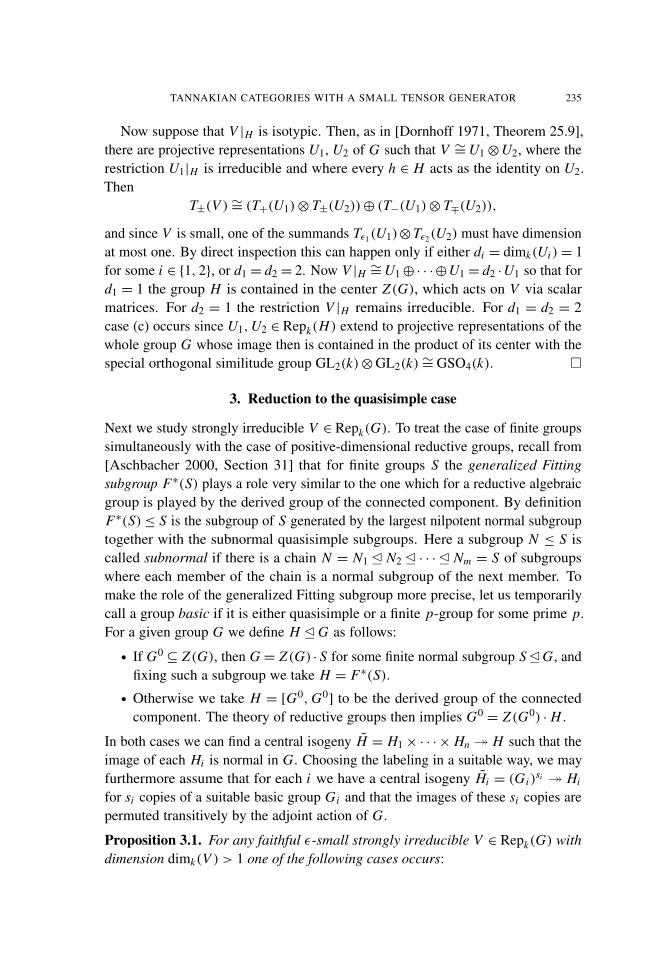
TANNAKIAN CATEGORIES WITH A SMALL TENSOR GENERATOR 235
Now suppose that V |H is isotypic. Then, as in [Dornhoff 1971, Theorem 25.9],there are projective representations U1, U2 of G such that V ∼=U1⊗U2, where therestriction U1|H is irreducible and where every h ∈ H acts as the identity on U2.Then
T±(V )∼= (T+(U1)⊗ T±(U2))⊕ (T−(U1)⊗ T∓(U2)),
and since V is small, one of the summands Tε1(U1)⊗Tε2(U2) must have dimensionat most one. By direct inspection this can happen only if either di = dimk(Ui )= 1for some i ∈ {1, 2}, or d1 = d2 = 2. Now V |H ∼=U1⊕· · ·⊕U1 = d2 ·U1 so that ford1 = 1 the group H is contained in the center Z(G), which acts on V via scalarmatrices. For d2 = 1 the restriction V |H remains irreducible. For d1 = d2 = 2case (c) occurs since U1,U2 ∈ Repk(H) extend to projective representations of thewhole group G whose image then is contained in the product of its center with thespecial orthogonal similitude group GL2(k)⊗GL2(k)∼= GSO4(k). �
3. Reduction to the quasisimple case
Next we study strongly irreducible V ∈ Repk(G). To treat the case of finite groupssimultaneously with the case of positive-dimensional reductive groups, recall from[Aschbacher 2000, Section 31] that for finite groups S the generalized Fittingsubgroup F∗(S) plays a role very similar to the one which for a reductive algebraicgroup is played by the derived group of the connected component. By definitionF∗(S)≤ S is the subgroup of S generated by the largest nilpotent normal subgrouptogether with the subnormal quasisimple subgroups. Here a subgroup N ≤ S iscalled subnormal if there is a chain N = N1E N2E · · ·E Nm = S of subgroupswhere each member of the chain is a normal subgroup of the next member. Tomake the role of the generalized Fitting subgroup more precise, let us temporarilycall a group basic if it is either quasisimple or a finite p-group for some prime p.For a given group G we define H EG as follows:
• If G0⊆ Z(G), then G = Z(G) · S for some finite normal subgroup SEG, and
fixing such a subgroup we take H = F∗(S).
• Otherwise we take H = [G0,G0] to be the derived group of the connected
component. The theory of reductive groups then implies G0= Z(G0) · H .
In both cases we can find a central isogeny H = H1× · · ·× Hn � H such that theimage of each Hi is normal in G. Choosing the labeling in a suitable way, we mayfurthermore assume that for each i we have a central isogeny Hi = (Gi )
si � Hi
for si copies of a suitable basic group Gi and that the images of these si copies arepermuted transitively by the adjoint action of G.
Proposition 3.1. For any faithful ε-small strongly irreducible V ∈ Repk(G) withdimension dimk(V ) > 1 one of the following cases occurs:

236 THOMAS KRÄMER AND RAINER WEISSAUER
(a) The group H is quasisimple.
(b) (H, V |H )∼= (G1⊗G1,W �W ) for some very small W ∈ Repk(G1), H flipsthe two factors, and we have ε =−1.
(c) H contains an extraspecial G-stable subgroup E of order p2n+1 for someprime p such that V |E is irreducible of dimension pn .
(d) We have an embedding G ↪→ GO4(k) such that V is the restriction of thefour-dimensional standard representation.
Proof. We first claim that H 6⊆ Z(G). Indeed, for the finite group case recall thatthe generalized Fitting subgroup contains its own centralizer [Aschbacher 2000],so H ⊆ Z(G) would imply S = H and then G = Z(G) would be abelian. In theinfinite case where G0 is not central, the strong irreducibility implies that V |G0 isirreducible so that the connected reductive group G0 cannot be a torus. Thus indeedH 6⊆ Z(G).
Hence we can assume that the image of each Hi in G is a noncentral subgroup bydiscarding any occurring central components and saturating the other componentswith the center. Since V |H ∼= U1� · · ·�Un with irreducible Ui ∈ Repk(Hi ), weget n = 1 by strong irreducibility. Hence H ∼= (G1)
s for s = s1 and again we geta decomposition V |H ∼=W1� · · ·�Ws with irreducible Wi ∈ Repk(G1), but nowthe adjoint action of G permutes the s factors G1 transitively so that all Wi areisomorphic to a single W ∈ Repk(G1). In the decomposition
Tε(V )|H ∼=s⊕
r=0
Tr,ε with Tr,ε =⊕
ε1···εs=ε#{i |εi=+1}=r
Tε1(W )� · · ·� Tεs (W )
each summand Tr,ε is stable under the action of G. By smallness it then followsthat s ≤ 2, and for s = 2 the conclusions of (b) or (d) hold.
So we may assume s = 1 and H = G1 is a basic group. If case (a) does notoccur, then H is a finite p-group for some prime p. Consider then a minimalG-stable noncentral subgroup M E H . By minimality the subgroup [M,M] iscontained in A := M ∩ Z(H) so that the quotient U := M/A is abelian. Lookingat the p-torsion part of this quotient one obtains, again by minimality, that U iselementary abelian. The commutator induces a bilinear map [·, ·] : U ×U → A,and if we identify A with a subgroup of Gm via Schur’s lemma, p ·U = 0 impliesthat [M,M] is contained in the subgroup µp ⊆ A of p-th roots of unity. So M/µp
is abelian and in fact elementary abelian: Otherwise by minimality its p-torsionsubgroup would lie in the cyclic group A/µp so that the abelian p-group M/µp
would be cyclic as well. But then M would be abelian, and this is impossible sinceit admits the faithful irreducible representation V |M of dimension d > 1.

TANNAKIAN CATEGORIES WITH A SMALL TENSOR GENERATOR 237
Thus M/µp is elementary abelian, and we claim that the extraspecial case (c)occurs. Indeed, either A = µp or A = µp2 . For A = µp the subgroup E = Msatisfies our requirements, so suppose that A = µp2 . Since M/µp is elementaryabelian, the Frattini subgroup is 8(M)= µp by [Aschbacher 2000, (23.2)]. TheFrattini subgroup is the intersection of all maximal subgroups, so it follows thatthere exists a maximal subgroup E ≤ M which contains µp but not µp2 . ThenM = µp2 · E , and E ≤ M is an extraspecial subgroup. We will be done if we canshow this subgroup is stable under the group AutA(M) of automorphisms of M thatare trivial on A. But this follows from the observation that every automorphism ofE which is trivial on µp extends uniquely to an element of AutA(M), which givesa natural identification AutA(M) ∼= Autµp(E) compatible with the actions on Mand E . �
We remark that the only instance of case (b) in Proposition 3.1 with dim(H) > 0is G1 ∼= SLm(k), acting on W ∼= km either via the standard representation or via itsdual. Indeed this will follow from Theorem 4.1 below, applied to the very smallrepresentation W of the Lie algebra of G1. Alternatively one could use [Guralnickand Tiep 2005].
In case (c) where H contains a G-stable extraspecial p-group E , put |E | = p1+2n
with n ∈ N. For any nontrivial character ω : Z(E) ∼= Z/pZ→ Gm there exists aunique irreducible representation Vω ∈ Repk(E) of dimension pn on which Z(E)acts via the character ω, and these are already all the irreducible representationsof dimension > 1 by [Dornhoff 1971, Theorem 31.5]. Hence in case (c) we haveV |E ∼= Vω for a uniquely determined character ω. To decide which of the occurringrepresentations are small, note that for the finite group S such that H = F∗(S),we have a natural homomorphism S→ Out(E). We now distinguish two casesdepending on p.
For p > 2 we have ω26= 1, so Tε(V )|E is an isotypic multiple of Vω2 . Then
Mackey theory [Dornhoff 1971, Theorem 25.9] gives a tensor product decompo-sition Tε(V ) ∼= U ⊗ Wε where U and Wε are projective representations of thegroup S such that U |E ∼= Vω2 and such that every element of E acts trivially on Wε .Via the nondegenerate alternating bilinear form defined by the commutator onE/Z(E)∼= (Fp)
2n we can identify the image of S in Out(E) with a subgroup of thesymplectic group Sp2n(Fp). Looking at dimensions one then obtains from [Tiep andZalesskii 1996, Theorem 5.2] that Wε must be one of the two Weil representationsof dimension (pn
+ ε)/2. Hence V is ε-small if and only if the image of S insideSp2n(Fp) acts irreducibly on this Weil representation.
For p = 2 on the other hand, ω2= 1, so that the restriction Tε(V )|E is a
sum of characters. By [Winter 1972] we can identify Out(E) with an orthogonalgroup O±2n(F2) where the type ± of the quadratic form depends on E . Recallthat a nondegenerate quadratic form on (F2)
2n has type ± if and only if there

238 THOMAS KRÄMER AND RAINER WEISSAUER
are precisely 2n−1(2n± 1) isotropic vectors for this form. One then obtains the
following identifications:
• If the quadratic form has + type, the isotropic vectors in (F2)2n correspond
precisely to the characters in T+(V )|E .
• If the quadratic form has − type, the isotropic vectors in (F2)2n correspond
precisely to the characters in T−(V )|E .
A similar interpretation holds for the anisotropic vectors. Hence it follows that V issmall if and only if the image of S inside O±2n(F2) acts transitively on the nonzeroisotropic resp. anisotropic vectors. Note that the set of isotropic vectors alwaysincludes the zero vector as a single orbit, corresponding to the trivial summand1 ↪→ Tε(V ).
4. Lie super algebras
It remains to determine all small V ∈ Repk(G) when H = [G0,G0] is quasisimple
and V |H is irreducible. By the classification of reductive super groups in [Weissauer2009], the Lie super algebra g of H must then either be an ordinary simple Liealgebra or an orthosymplectic Lie super algebra osp1|2m(k) with m ∈ N. Note thatRepk(H) is a full subcategory of Repk(g), where the latter denotes the categoryof all Lie algebra representations of the Lie super algebra g on finite-dimensionalsuper vector spaces over k. In particular V |H defines an irreducible representationof g.
The passage to representations of Lie algebras leads to a seemingly weaker notionof smallness. By the comments after Theorem 1.1 we know that G/(G0
· ZG(G0))
is a subgroup of Out(G0) such that conjugation by any element ϕ of this subgroupfixes the isomorphism type of V |H . For an irreducible summand W ↪→ Tε(V )in Repk(G) it may happen that the restriction W |H splits into several irreduciblesummands, but all these summands must be conjugate via automorphisms ϕ asabove. Abstracting from this situation, let us now denote by g any ordinary simpleLie algebra or osp1|2m(k) with m ∈ N. We say that a representation V ∈ Repk(g)
is ε-small if either Tε(V )∼=W or Tε(V )∼=W ⊕1, where W is a sum of irreduciblerepresentations which are all conjugate to each other via automorphisms ϕ ∈Aut(g)fixing the isomorphism type of V . To finish the proof of Theorem 1.1 we classifyall irreducible small representations in this sense. For a uniform treatment the termsdimension, vector space, trace and Lie algebra will from now on be taken in thesuper sense for osp1|2m(k) but in the ordinary sense otherwise.
We denote by $1, . . . ,$m the fundamental dominant weights of g with respectto some fixed system of simple positive roots; see [Rittenberg and Scheunert 1982,Section 2.1] for the orthosymplectic Lie algebra g= osp1|2m(k) whose Dynkin type

TANNAKIAN CATEGORIES WITH A SMALL TENSOR GENERATOR 239
we abbreviate by BCm . Put
βi =
{2$m if g= osp1|2m(k) and i = m,$i otherwise.
The irreducible finite-dimensional representations of g are parametrized by highestweights λ=
∑mi=1 aiβi with ai ∈N0, see [Djokovic 1976b, Theorem 6]. For any such
λ we denote by Vλ the associated positive-dimensional irreducible representation.Note that, in the super case, negative-dimensional irreducible representations areobtained by the parity flip Wλ =5Vλ with dim(Wλ)=− dim(Vλ) and S2(Wλ)∼=
32(Vλ).
Theorem 4.1. A positive-dimensional irreducible representation Vλ ∈ Repk(g) isε-small if and only if its highest weight λ appears in the following table:
λ ε =+1 ε =−1Am m ≥ 1 β1, βm ? ?
m = 1 2β1 ◦ ?
3β1 − ◦
m ≥ 2 2β1, 2βm − ?
m = 3 β2 ◦ ?
m ≥ 4 β2, βm−1 − ?
m = 5 β3 − ◦
Bm m ≥ 2 β1 ◦ ?
m = 2 β2 ? ◦
m = 3 β3 ◦ −
Cm m ≥ 3 β1 ? ◦
m = 3 β3 − ◦
Dm m ≥ 4 β1 ◦ ?
m = 4 β3, β4 ◦ ?
m = 5 β4, β5 − ?
m = 6 β5, β6 − ◦
BCm m ≥ 1 β1 ? ◦
E6 β1, β6 − ?
E7 β7 − ◦
G2 β1 ◦ −
Here the label ? means that Tε(Vλ) is irreducible, ◦ means that Tε(Vλ) = W ⊕ 1with W irreducible, and − means that Vλ is not ε-small.
Note that for g= sl2(k) with its two-dimensional standard representation st , anyirreducible representation is a symmetric power Vλ = Sn(st) of weight λ = nβ1
for some n ∈ N. In this case Theorem 4.1 holds by direct inspection. A similar

240 THOMAS KRÄMER AND RAINER WEISSAUER
argument also works for g = osp1|2(k). Here we know from [Djokovic 1976b,Theorems 7 and 11] that for λ = nβ1 the even subalgebra g0 = sl2(k) ⊂ g actson Vλ = V0⊕ V1 via V0 = Sn(st) and V1 = Sn−1(st). A short computation yieldsthe action on the even and odd parts of the tensor square Tε(V ) and Theorem 4.1also holds in this case. Note that dim(V )= 1 for all irreducible representations Vof osp1|2(k). For all other cases we have:
Lemma 4.2. For g 6= osp1|2(k) one has dim(Vλ)≤ dim(g) if and only if the highestweight λ appears among those listed in Tables 1 or 2.
Proof. See [Andreev et al. 1967] for the ordinary case. For g=osp1|2m(k)with m≥2we use the Kac–Weyl formula in [Tsohantjis and Cornwell 1990, Equation 11]. Weembed the root system BCm into a Euclidean space with standard basis ε1, . . . , εm
such that βi = ε1+ · · ·+ εi for all i . The irreducible representations of osp1|2m(k)are parametrized by weights which in our basis are written λ= (λ1, . . . , λm) withintegers λ1 ≥ · · · ≥ λm ≥ 0. The Kac–Weyl formula gives
dim(Vλ) =∏
1≤i< j≤m
(λi − λ j
j − i+ 1
)·
∏1≤i< j≤m
(λi + λ j
2m+ 1− i − j+ 1
).
For λ1 ≥ 2 the second product is ≥ 2. Then the classical Weyl formula for thefirst product shows that dim(Vλ) is at least twice the dimension of the irreduciblerepresentation of slm(k) with highest weight µ= (λ1−λm, . . . , λm−1−λm). Usingthat dim(slm(k)) ≥ 2 dim(osp1|2m(k)), it follows that µ is in the list for Am−1 inTable 1. Since λ = µ+ λm · βm and since increasing the weight by βm increasesthe dimension, this leaves only finitely many cases. For λ1 = 1 we have λ = βr
λ S2(Vλ) 32(Vλ)Am m = 1 β1 V2β1 1
m ≥ 2 β1 V2β1 Vβ2
βm V2βm Vβm−1
m ≥ 2 2β1 V4β1 ⊕ V2β2 V2β1+β2
2βm V4βm ⊕ V2βm−1 V2βm+βm−1
m ≥ 4 β2 V2β2 ⊕ Vβ4 Vβ1+β3
βm−1 V2βm−1 ⊕ Vβm−3 Vβm+βm−2
m = 3 β2 V2β2 ⊕ 1 Vβ1+β3
m = 5 β3 V2β3 ⊕ Vβ1+β5 Vβ2+β4 ⊕ 1m = β3 V2β3 ⊕ Vβ1+β5 Vβ2+β4 ⊕ Vβ6
6, 7 βm−2 V2βm−2 ⊕ Vβm+βm−4 Vβm−1+βm−3 ⊕ Vβm−5
Table 1. All λ with 1 < dim(Vλ) < dim(g). For g = osp1|2m(k)we denote by Wµ = 5Vµ the parity shifts of the highest weightmodules. (Continues on the next page.)
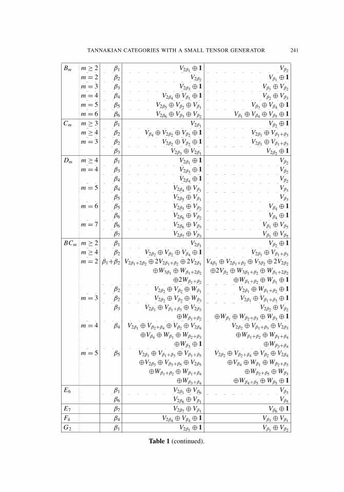
TANNAKIAN CATEGORIES WITH A SMALL TENSOR GENERATOR 241
Bm m ≥ 2 β1 V2β1 ⊕ 1 Vβ2
m = 2 β2 V2β2 Vβ1 ⊕ 1m = 3 β3 V2β3 ⊕ 1 Vβ1 ⊕ Vβ2
m = 4 β4 V2β4 ⊕ Vβ1 ⊕ 1 Vβ2 ⊕ Vβ3
m = 5 β5 V2β5 ⊕ Vβ2 ⊕ Vβ1 Vβ3 ⊕ Vβ4 ⊕ 1m = 6 β6 V2β6 ⊕ Vβ3 ⊕ Vβ2 Vβ1 ⊕ Vβ4 ⊕ Vβ5 ⊕ 1
Cm m ≥ 3 β1 V2β1 Vβ2 ⊕ 1m ≥ 4 β2 Vβ4 ⊕ V2β2 ⊕ Vβ2 ⊕ 1 V2β1 ⊕ Vβ1+β3
m = 3 β2 V2β2 ⊕ Vβ2 ⊕ 1 V2β1 ⊕ Vβ1+β3
β3 V2β3 ⊕ V2β1 V2β2 ⊕ 1Dm m ≥ 4 β1 V2β1 ⊕ 1 Vβ2
m = 4 β3 V2β3 ⊕ 1 Vβ2
β4 V2β4 ⊕ 1 Vβ2
m = 5 β4 V2β4 ⊕ Vβ1 Vβ3
β5 V2β5 ⊕ Vβ1 Vβ3
m = 6 β5 V2β5 ⊕ Vβ2 Vβ4 ⊕ 1β6 V2β6 ⊕ Vβ2 Vβ4 ⊕ 1
m = 7 β6 V2β6 ⊕ Vβ3 Vβ1 ⊕ Vβ5
β7 V2β7 ⊕ Vβ3 Vβ1 ⊕ Vβ5
BCm m ≥ 2 β1 V2β1 Vβ2 ⊕ 1m ≥ 4 β2 V2β2 ⊕ Vβ2 ⊕ Vβ4 ⊕ 1 V2β1 ⊕ Vβ1+β3
m = 2 β1+β2 V2β1+2β2 ⊕ 2V2β1+β2 ⊕ 2V2β1 V4β1 ⊕ V2β1+β2 ⊕ V3β2 ⊕ 2V2β2
⊕W3β1 ⊕Wβ1+2β2 ⊕2Vβ2 ⊕W3β1+β2 ⊕Wβ1+2β2
⊕2Wβ1+β2 ⊕Wβ1+β2 ⊕Wβ1 ⊕ 1β2 V2β2 ⊕ Vβ2 ⊕Wβ1 V2β1 ⊕Wβ1+β2 ⊕ 1
m = 3 β2 V2β2 ⊕ Vβ2 ⊕Wβ3 V2β1 ⊕ Vβ1+β3 ⊕ 1β3 V2β1 ⊕ Vβ1+β3 ⊕ V2β3 V2β2 ⊕ Vβ2
⊕Wβ1+β2 ⊕Wβ1 ⊕Wβ2+β3 ⊕Wβ3 ⊕ 1m = 4 β4 V2β1 ⊕ Vβ2+β4 ⊕ Vβ2 ⊕ V2β4 V2β2 ⊕ Vβ1+β3 ⊕ V2β3
⊕Vβ4 ⊕Wβ1 ⊕Wβ2+β3 ⊕Wβ1+β2 ⊕Wβ1+β4
⊕Wβ3 ⊕ 1 ⊕Wβ3+β4
m = 5 β5 V2β1 ⊕ Vβ1+β3 ⊕ Vβ1+β5 V2β2 ⊕ Vβ2+β4 ⊕ Vβ2 ⊕ V2β4
⊕V2β3 ⊕ Vβ3+β5 ⊕ V2β5 ⊕Vβ4 ⊕Wβ1 ⊕Wβ2+β3
⊕Wβ1+β2 ⊕Wβ1+β4 ⊕Wβ2+β5 ⊕Wβ3
⊕Wβ3+β4 ⊕Wβ4+β5 ⊕Wβ5 ⊕ 1E6 β1 V2β1 ⊕ Vβ6 Vβ3
β6 V2β6 ⊕ Vβ1 Vβ5
E7 β7 V2β7 ⊕ Vβ1 Vβ6 ⊕ 1F4 β4 V2β4 ⊕ Vβ4 ⊕ 1 Vβ3 ⊕ Vβ1
G2 β1 V2β1 ⊕ 1 Vβ1 ⊕ Vβ2
Table 1 (continued).

242 THOMAS KRÄMER AND RAINER WEISSAUER
λ S2(Vλ) 32(Vλ)Am m = 1 2β1 V4β1 ⊕ 1 V2β1
m = 2 β1+β2 V2β1+2β2 ⊕ Vβ1+β2 ⊕ 1 V3β1 ⊕ V3β2 ⊕ Vβ1+β2
m ≥ 2 β1+βm V2β1+2βm ⊕ Vβ2+βm−1 Vβ2+2βm ⊕ V2β1+βm−1
⊕Vβ1+βm ⊕ 1 ⊕Vβ1+βm
Bm m = 2 2β2 Vβ1 ⊕ V2β1 ⊕ V4β2 ⊕ 1 Vβ1+2β2 ⊕ V2β2
m = 3 β2 V2β1 ⊕ V2β2 ⊕ V2β3 ⊕ 1 Vβ1+2β3 ⊕ Vβ2
m = 4 β2 V2β1 ⊕ V2β2 ⊕ V2β4 ⊕ 1 Vβ1+β3 ⊕ Vβ2
m ≥ 5 β2 V2β1 ⊕ V2β2 ⊕ Vβ4 ⊕ 1 Vβ1+β3 ⊕ Vβ2
Cm m ≥ 3 2β1 V4β1 ⊕ V2β2 ⊕ Vβ2 ⊕ 1 V2β1 ⊕ V2β1+β2
Dm m = 4 β2 V2β1 ⊕ V2β2 ⊕ V2β3 ⊕ V2β4 ⊕ 1 Vβ2 ⊕ Vβ1+β3+β4
m = 5 β2 V2β1 ⊕ V2β2 ⊕ Vβ4+β5 ⊕ 1 Vβ2 ⊕ Vβ1+β3
m ≥ 6 β2 V2β1 ⊕ V2β2 ⊕ Vβ4 ⊕ 1 Vβ2 ⊕ Vβ1+β3
BCm m ≥ 2 2β1 V4β1 ⊕ V2β2 ⊕ Vβ2 ⊕ 1 V2β1+β2 ⊕ V2β1
m = 4 β3 V2β1 ⊕ Vβ1+β3 ⊕ V2β3 V2β2 ⊕ Vβ2 ⊕ Vβ2+β4
⊕Wβ1+β4 ⊕Vβ4 ⊕Wβ3 ⊕ 1E6 β2 V2β2 ⊕ Vβ1+β6 ⊕ 1 Vβ2 ⊕ Vβ4
E7 β1 V2β1 ⊕ Vβ6 ⊕ 1 Vβ1 ⊕ Vβ3
E8 β8 Vβ1 ⊕ V2β8 ⊕ 1 Vβ7 ⊕ Vβ8
F4 β1 V2β1 ⊕ V2β4 ⊕ 1 Vβ1 ⊕ Vβ2
G2 β2 V2β1 ⊕ V2β2 ⊕ 1 V3β1 ⊕ Vβ2
Table 2. All λ with 1 < dim(Vλ) = dim(g). For the ordinarysimple Lie algebras precisely the adjoint representations occur bythe result of [Andreev et al. 1967].
with r ≤ m, and dim(Vλ) =(2m
r
)−( 2m
r−1
)by the description in [Djokovic 1976b,
Section 5]. �
Corollary 4.3. For g 6= sl2(k), osp1|2(k) and all weights λ one has dim(Vλ) ≥ 2,with equality holding only in the single case (g, λ)= (osp1|4(k), β2).
5. Proof of Theorem 4.1
Recall that g admits a unique invariant nondegenerate bilinear form (·, ·) up tomultiplication by a scalar [Scheunert 1979, p. 94]. Fixing any such form, weassociate to any root α a coroot α∨ = 2α/(α, α). Let α1, . . . , αm be a system ofsimple positive roots so that the fundamental weights $i satisfy (α∨i ,$ j ) = δi j .Then ρ = $1 + · · · + $m is half the sum of all positive roots, with the signconvention of [Tsohantjis and Cornwell 1990]. For the proof of Theorem 4.1 weconsider the index of a representation ϕ : g→ gl(V ), i.e., the scalar l(V ) definedby tr(ϕ(X) ◦ϕ(Y ))= l(V ) · (X, Y ).

TANNAKIAN CATEGORIES WITH A SMALL TENSOR GENERATOR 243
Lemma 5.1. The index has the following properties.
(a) For the symmetric or alternating square of a representation V it is given bythe formula l(Tε(V ))= (dim(V )+ 2ε) · l(V ).
(b) There exists a constant κ 6= 0 such that κ ·l(Vµ)= dim(Vµ) ·c(µ) for the scalarc(µ)= (µ,µ)+ 2(µ, ρ) > 0 and for any highest weight µ 6= 0.
(c) The index satisfies l(1) = 0, and it is invariant under automorphisms andadditive for direct sums in the sense that l(V ⊕ V ′)= l(V )+ l(V ′).
Proof. For (a) note that upon applying any tensor construction to V the index ismultiplied by a constant depending only on n = dim(V ). To compute this constantfor Tε(V ), recall from [Scheunert 1979, p. 128] that sl(V ) is simple for n 6= 0. Itthen only remains to check that tr((Tε(X))2)= (n+2ε) tr(X2) for a suitably chosenelementary matrix X ∈ sl(V ). For (b) one checks, by looking at the action on ahighest weight vector, that the Casimir operator acts on Vµ by some fixed multipleof c(µ). The setting for osp1|2m(k) is described in [Djokovic 1976b, p. 28; 1976a,p. 223]. One then has κ = dim(Ad) · c(Ad) for the adjoint representation Ad. Part(c) is obvious. �
Via these index computations, we may now complete the classification of ε-smallrepresentations for g 6= sl2(k), osp1|2(k) as follows.
Proof of Theorem 4.1. Suppose that Vλ is ε-small. By Corollary 4.3 we mayassume that n = dim(Vλ) > 2. Put Tε(Vλ)=W ⊕ 1δ where δ ∈ {0, 1} denotes themultiplicity with which the trivial representation enters. Note that by smallnessall highest weights µ occurring in W are conjugate to each other. For any such µLemma 5.1(b)–(c) hence imply that κ ·l(W )=dim(W )·c(µ)= (n(n+ε)/2−δ)·c(µ)and κ · l(Vλ)= n · c(λ). So Lemma 5.1(a) shows
(?) (n+ 2ε) · n · c(λ)= 12
(n(n+ ε)− 2δ
)· c(µ).
Now we distinguish between the symmetric and the alternating square. For ε=+1we may take µ = 2λ. Then c(µ) = 4|λ|2+ 4(λ, ρ). Since c(λ) = |λ|2+ 2(λ, ρ),Equation (?) easily gives
(n− 2δ) · |λ|2 = 2(λ, ρ) and hence |λ| ≤2|ρ|
n− 2δ
by the Cauchy–Schwartz inequality. Let 10 be the set of simple positive roots ofthe even subalgebra g0. Then
|(λ, α∨)| ≤ |λ| · |α∨| ≤2 |ρ||α∨|
n− 2δ<
dim(g)− 1n− 2δ
for any α ∈10,
where for the last inequality we have used the numerical values of |ρ|2 and R inTable 3 and our assumption g 6= sl2(k), osp1|2(k). On the other hand (λ, α∨) ∈ Z

244 THOMAS KRÄMER AND RAINER WEISSAUER
|ρ|2 R dim(g) ri for i = 1, . . . ,m |Out(g)|
Amm(m+1)(m+2)
12
√2 m(m+ 2) 2(m+1)
i(m+1−i) 2
Bmm(2m−1)(2m+1)
12 2 m(2m+ 1) 2i (1+ δim) 1
Cmm(m+1)(2m+1)
6
√2 m(2m+ 1) 2
i (1+ δim) 1
Dmm(m−1)(2m−1)
6
√2 m(2m− 1) 2
i if i < m− 1 2 if m 6= 48m if i ∈ {m− 1,m} 6 if m = 4
BCmm(2m−1)(2m+1)
12
√2 m(2m− 1) 2
i (1+ δim) 1
E6 78√
2 78 32 , 1, 3
5 ,13 ,
35 ,
32 2
E7399
2
√2 133 1, 4
7 ,13 ,
16 ,
415 ,
12 ,
43 1
E8 620√
2 248 12 ,
14 ,
17 ,
115 ,
110 ,
16 ,
13 , 1 1
F4 39 2 52 1, 13 ,
13 , 1 1
G2 14√
2 14 1 1
Table 3. Some numerical values. We put ri = |αi |2/|βi |
2 andR =maxα∈10 |α
∨| for the set 10 of simple positive roots of g0.
for all α ∈10, and for λ 6= 0 at least one of these scalar products is nonzero. Thuswe can find α ∈10 with |(λ, α∨)| ≥ 1. This implies n−2δ < dim(g)−1. Hence λis one of the highest weights in tables 1 and 2 by Lemma 4.2.
It remains to discuss the case ε=−1. By smallness all highest weights in32(Vλ)are conjugate to each other via automorphisms fixing λ. Hence Remark 5.2 belowimplies
(??) λ= r · (βi1 + · · ·+βis ) for some r ∈ N and i1 < i2 < · · ·< is,
and that for all i ∈ {i1, . . . , is} the weight µ= 2λ−αi occurs as a highest weight in32(Vλ). In what follows we fix i ∈ {i1, . . . , is} with the smallest norm |βi |. Sincethe norm of any simple positive root is given by the formula |αi |
2= 2 (αi , ρ), we
have c(µ)/2= c(λ)+ |λ|2− 2(λ, αi ) so that (?) becomes
(n+ 2ε) · n · c(λ)=(n(n+ ε)− 2δ
)·(c(λ)+ |λ|2− 2(λ, αi )
).
Now for ε =−1 the first of the two factors on the right is > (n+ 2ε) · n since byassumption n > 2 and δ ∈ {0, 1}. Hence
c(λ)+ |λ|2− 2(λ, αi ) < c(λ)
and therefore 2 (λ, αi ) > |λ|2≥ r2· |βi |
2· s, where the second inequality comes
from (??) together with the fact that all scalar products between βi1, . . . , βis arenonnegative and βi has the smallest norm among all these weights. On the other
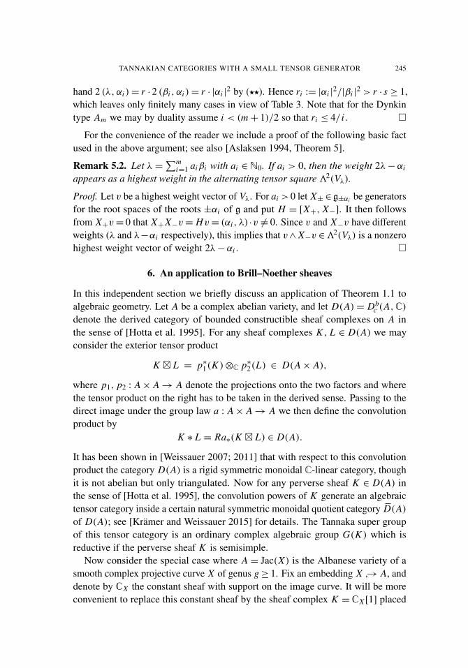
TANNAKIAN CATEGORIES WITH A SMALL TENSOR GENERATOR 245
hand 2 (λ, αi )= r · 2 (βi , αi )= r · |αi |2 by (??). Hence ri := |αi |
2/|βi |2 > r · s ≥ 1,
which leaves only finitely many cases in view of Table 3. Note that for the Dynkintype Am we may by duality assume i < (m+ 1)/2 so that ri ≤ 4/ i . �
For the convenience of the reader we include a proof of the following basic factused in the above argument; see also [Aslaksen 1994, Theorem 5].
Remark 5.2. Let λ =∑m
i=1 aiβi with ai ∈ N0. If ai > 0, then the weight 2λ− αi
appears as a highest weight in the alternating tensor square 32(Vλ).
Proof. Let v be a highest weight vector of Vλ. For ai > 0 let X± ∈g±αi be generatorsfor the root spaces of the roots ±αi of g and put H = [X+, X−]. It then followsfrom X+v= 0 that X+X−v= Hv= (αi , λ) ·v 6= 0. Since v and X−v have differentweights (λ and λ−αi respectively), this implies that v∧X−v ∈32(Vλ) is a nonzerohighest weight vector of weight 2λ−αi . �
6. An application to Brill–Noether sheaves
In this independent section we briefly discuss an application of Theorem 1.1 toalgebraic geometry. Let A be a complex abelian variety, and let D(A)= Db
c (A,C)
denote the derived category of bounded constructible sheaf complexes on A inthe sense of [Hotta et al. 1995]. For any sheaf complexes K , L ∈ D(A) we mayconsider the exterior tensor product
K � L = p∗1(K )⊗C p∗2(L) ∈ D(A× A),
where p1, p2 : A× A→ A denote the projections onto the two factors and wherethe tensor product on the right has to be taken in the derived sense. Passing to thedirect image under the group law a : A× A→ A we then define the convolutionproduct by
K ∗ L = Ra∗(K � L) ∈ D(A).
It has been shown in [Weissauer 2007; 2011] that with respect to this convolutionproduct the category D(A) is a rigid symmetric monoidal C-linear category, thoughit is not abelian but only triangulated. Now for any perverse sheaf K ∈ D(A) inthe sense of [Hotta et al. 1995], the convolution powers of K generate an algebraictensor category inside a certain natural symmetric monoidal quotient category D(A)of D(A); see [Krämer and Weissauer 2015] for details. The Tannaka super groupof this tensor category is an ordinary complex algebraic group G(K ) which isreductive if the perverse sheaf K is semisimple.
Now consider the special case where A = Jac(X) is the Albanese variety of asmooth complex projective curve X of genus g≥ 1. Fix an embedding X ↪→ A, anddenote by CX the constant sheaf with support on the image curve. It will be moreconvenient to replace this constant sheaf by the sheaf complex K = CX [1] placed
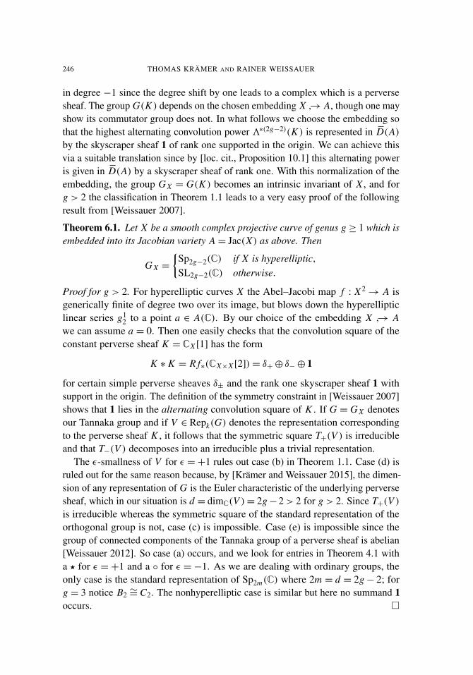
246 THOMAS KRÄMER AND RAINER WEISSAUER
in degree −1 since the degree shift by one leads to a complex which is a perversesheaf. The group G(K ) depends on the chosen embedding X ↪→ A, though one mayshow its commutator group does not. In what follows we choose the embedding sothat the highest alternating convolution power 3∗(2g−2)(K ) is represented in D(A)by the skyscraper sheaf 1 of rank one supported in the origin. We can achieve thisvia a suitable translation since by [loc. cit., Proposition 10.1] this alternating poweris given in D(A) by a skyscraper sheaf of rank one. With this normalization of theembedding, the group G X = G(K ) becomes an intrinsic invariant of X , and forg > 2 the classification in Theorem 1.1 leads to a very easy proof of the followingresult from [Weissauer 2007].
Theorem 6.1. Let X be a smooth complex projective curve of genus g ≥ 1 which isembedded into its Jacobian variety A = Jac(X) as above. Then
G X =
{Sp2g−2(C) if X is hyperelliptic,SL2g−2(C) otherwise.
Proof for g > 2. For hyperelliptic curves X the Abel–Jacobi map f : X2→ A is
generically finite of degree two over its image, but blows down the hyperellipticlinear series g1
2 to a point a ∈ A(C). By our choice of the embedding X ↪→ Awe can assume a = 0. Then one easily checks that the convolution square of theconstant perverse sheaf K = CX [1] has the form
K ∗ K = R f∗(CX×X [2])= δ+⊕ δ−⊕ 1
for certain simple perverse sheaves δ± and the rank one skyscraper sheaf 1 withsupport in the origin. The definition of the symmetry constraint in [Weissauer 2007]shows that 1 lies in the alternating convolution square of K . If G = G X denotesour Tannaka group and if V ∈ Repk(G) denotes the representation correspondingto the perverse sheaf K , it follows that the symmetric square T+(V ) is irreducibleand that T−(V ) decomposes into an irreducible plus a trivial representation.
The ε-smallness of V for ε =+1 rules out case (b) in Theorem 1.1. Case (d) isruled out for the same reason because, by [Krämer and Weissauer 2015], the dimen-sion of any representation of G is the Euler characteristic of the underlying perversesheaf, which in our situation is d = dimC(V )= 2g−2> 2 for g > 2. Since T+(V )is irreducible whereas the symmetric square of the standard representation of theorthogonal group is not, case (c) is impossible. Case (e) is impossible since thegroup of connected components of the Tannaka group of a perverse sheaf is abelian[Weissauer 2012]. So case (a) occurs, and we look for entries in Theorem 4.1 witha ? for ε = +1 and a ◦ for ε = −1. As we are dealing with ordinary groups, theonly case is the standard representation of Sp2m(C) where 2m = d = 2g− 2; forg = 3 notice B2 ∼= C2. The nonhyperelliptic case is similar but here no summand 1occurs. �

TANNAKIAN CATEGORIES WITH A SMALL TENSOR GENERATOR 247
References
[André and Kahn 2002] Y. André and B. Kahn, “Nilpotence, radicaux et structures monoïdales”, Rend.Sem. Mat. Univ. Padova 108 (2002), 107–291. Correction in 113 (2005), 125–128. MR 2003m:18009Zbl 1165.18300
[Andreev et al. 1967] E. M. Andreev, È. B. Vinberg, and A. G. Élashvili, “Orbity naibol~xeirazmernosti poluprostyh lineinyh grupp Li”, Funkcional. Anal. i Priložen. 1:4 (1967),3–7. Translated as “Orbits of greatest dimension in semi-simple linear Lie groups” in Funct. Anal.Appl 1:4 (1967), 257–261. MR 42 #1942 Zbl 0176.30301
[Aschbacher 2000] M. Aschbacher, Finite group theory, 2nd ed., Cambridge Studies in AdvancedMathematics 10, Cambridge University Press, 2000. MR 2001c:20001 Zbl 0997.20001
[Aslaksen 1994] H. Aslaksen, “Determining summands in tensor products of Lie algebra representa-tions”, J. Pure Appl. Algebra 93:2 (1994), 135–146. MR 95b:17008 Zbl 0815.17006
[Deligne 2002] P. Deligne, “Catégories tensorielles”, Mosc. Math. J. 2:2 (2002), 227–248. MR 2003k:18010 Zbl 1005.18009
[Deligne et al. 1982] P. Deligne, J. S. Milne, A. Ogus, and K.-Y. Shih, Hodge cycles, motives, andShimura varieties, Lecture Notes in Mathematics 900, Springer, Berlin, 1982. MR 84m:14046Zbl 0465.00010
[Dixon and Mortimer 1996] J. D. Dixon and B. Mortimer, Permutation groups, Graduate Texts inMathematics 163, Springer, New York, 1996. MR 98m:20003 Zbl 0951.20001
[Djokovic 1976a] D. Ž. Djokovic, “Classification of some 2-graded Lie algebras”, J. Pure Appl.Algebra 7:2 (1976), 217–230. MR 52 #10822 Zbl 0319.17005
[Djokovic 1976b] D. Ž. Djokovic, “Representation theory for symplectic 2-graded Lie algebras”, J.Pure Appl. Algebra 9:1 (1976), 25–38. MR 54 #10353 Zbl 0344.17005
[Dornhoff 1971] L. Dornhoff, Group representation theory, A: Ordinary representation theory, Pureand Applied Mathematics 7, Marcel Dekker, New York, 1971. MR 50 #458a Zbl 0227.20002
[Gabber and Loeser 1996] O. Gabber and F. Loeser, “Faisceaux pervers l-adiques sur un tore”, DukeMath. J. 83:3 (1996), 501–606. MR 97i:14016 Zbl 0896.14009
[Guralnick and Tiep 2005] R. M. Guralnick and P. H. Tiep, “Decompositions of small tensor powersand Larsen’s conjecture”, Represent. Theory 9 (2005), 138–208. MR 2006a:20082 Zbl 1109.20040
[Hotta et al. 1995] R. Hotta, K. Takeuchi, and T. Tanisaki, D-modules, perverse sheaves, andrepresentation theory, Springer, Tokyo, 1995. In Japanese; translated in Progress in Mathematics236, Birkhäuser, Boston, 2008. MR 2008k:32022 Zbl 1136.14009
[Kantor 1969] W. M. Kantor, “Automorphism groups of designs”, Math. Z. 109 (1969), 246–252.MR 43 #71 Zbl 0212.03504
[Kantor 1972] W. M. Kantor, “k-Homogeneous groups”, Math. Z. 124 (1972), 261–265. MR 46#5422 Zbl 0232.20003
[Krämer 2014] T. Krämer, “Perverse sheaves on semiabelian varieties”, Rend. Sem. Mat. Univ. Padova132 (2014), 83–102. MR 3276828 Zbl 06379718
[Krämer and Weissauer 2013] T. Krämer and R. Weissauer, “On the Tannaka group attached tothe theta divisor of a generic principally polarized abelian variety”, 2013. To appear in Math. Z.arXiv 1309.3754
[Krämer and Weissauer 2015] T. Krämer and R. Weissauer, “Vanishing theorems for constructiblesheaves on abelian varieties”, J. Alg. Geom. 24:3 (2015), 531–568.
[Magaard and Malle 1998] K. Magaard and G. Malle, “Irreducibility of alternating and symmetricsquares”, Manuscripta Math. 95:2 (1998), 169–180. MR 99a:20011 Zbl 0919.20009

248 THOMAS KRÄMER AND RAINER WEISSAUER
[Magaard et al. 2002] K. Magaard, G. Malle, and P. H. Tiep, “Irreducibility of tensor squares, sym-metric squares and alternating squares”, Pacific J. Math. 202:2 (2002), 379–427. MR 2002m:20025Zbl 1072.20013
[Rittenberg and Scheunert 1982] V. Rittenberg and M. Scheunert, “A remarkable connection betweenthe representations of the Lie superalgebras osp(1, 2n) and the Lie algebras o(2n + 1)”, Comm.Math. Phys. 83:1 (1982), 1–9. MR 83c:17021 Zbl 0479.17001
[Scheunert 1979] M. Scheunert, The theory of Lie superalgebras: an introduction, Lecture Notes inMathematics 716, Springer, Berlin, 1979. MR 80i:17005 Zbl 0407.17001
[Tiep and Zalesskii 1996] P. H. Tiep and A. E. Zalesskii, “Minimal characters of the finite classicalgroups”, Comm. Algebra 24:6 (1996), 2093–2167. MR 97f:20018 Zbl 0901.20031
[Tsohantjis and Cornwell 1990] I. Tsohantjis and J. F. Cornwell, “Supercharacters and superdimen-sions of irreducible representations of B(0/s) orthosymplectic simple Lie superalgebras”, Internat.J. Theoret. Phys. 29:4 (1990), 351–359. MR 91i:17007 Zbl 0702.17003
[Weissauer 2007] R. Weissauer, “Brill–Noether sheaves”, 2007. arXiv math/0610923
[Weissauer 2008] R. Weissauer, “Torelli’s theorem from the topological point of view”, pp. 275–284in Modular forms on Schiermonnikoog, edited by B. Edixhoven et al., Cambridge University Press,2008. MR 2011g:14020 Zbl 1156.14303
[Weissauer 2009] R. Weissauer, “Semisimple algebraic tensor categories”, 2009. arXiv 0909.1793
[Weissauer 2011] R. Weissauer, “A remark on rigidity of BN-sheaves”, 2011. arXiv 1111.6095
[Weissauer 2012] R. Weissauer, “Why certain Tannaka groups attached to abelian varieties are almostconnected”, 2012. arXiv 1207.4039
[Winter 1972] D. L. Winter, “The automorphism group of an extraspecial p-group”, Rocky MountainJ. Math. 2:2 (1972), 159–168. MR 45 #6911 Zbl 0242.20023
Received March 5, 2014. Revised November 6, 2014.
THOMAS KRÄMER
CENTRE DE MATHÉMATIQUES LAURENT SCHWARTZ
ÉCOLE POLYTECHNIQUE
F-91128 PALAISEAU CEDEX
FRANCE
RAINER WEISSAUER
MATHEMATISCHES INSTITUT
RUPRECHT-KARLS-UNIVERSITÄT HEIDELBERG
IM NEUENHEIMER FELD 288D-69120 HEIDELBERG
GERMANY
PACIFIC JOURNAL OF MATHEMATICSVol. 276, No. 1, 2015
dx.doi.org/10.2140/pjm.2015.276.249
ON MAXIMAL LINDENSTRAUSS SPACES
PETR PETRÁCEK AND JIRÍ SPURNÝ
We solve a problem of Lacey (1973) by showing that there exist a metrizablecompact space K and a closed space H ⊂ C(K ) containing constants with∂HK = K such that H is maximal with respect to ∂HK and H is not aLindenstrauss space.
1. Introduction
Let X be a compact convex subset of a real locally convex space and let Ac(X)denote the space of all affine continuous functions on X . Denote by ext X the setof all extreme points of X .
Let K be a compact Hausdorff topological space and H⊂C(K ) a closed subspaceof C(K ) containing constants and separating points of K . The space H can beidentified with Ac(X), where
X = {s∗ ∈H∗ : s∗(1)= ‖s∗‖ = 1}
with the weak* topology. Consider the set
∂HK = {x ∈ K : εx |H is an extreme point of the unit ball of H∗},
where εx denotes the Dirac measure at x ∈ K . Then ext X is homeomorphic to ∂HKvia the evaluation mapping (see Theorem 2.1 and [LMNS 2010, Proposition 4.26]).
The space H is called maximal with respect to ∂HK if for every closed space Gwith H⊂ G ⊂ C(K ) we have H= G provided ∂HK = ∂GK .
(In [Lacey 1973], the property of separating points is not a part of the definitionof a function space. Nevertheless, in our opinion, this property is necessary for∂HK to be homeomorphic to ext X . Indeed, consider H= span{1} on [0, 1]. ThenX is a singleton, and thus ∂H[0, 1] = [0, 1]. Obviously, [0, 1] is not homeomorphicto ext X .)
It is shown in [Edwards and Vincent-Smith 1968] that H is maximal with respectto ∂HK whenever H is a Lindenstrauss space; see Theorems 2.1 and 2.3 below.
The research was supported by grant GACR P201/12/0290. Spurný was also supported by the NeuronFund for Support of Science.MSC2010: 46B25.Keywords: Lindenstrauss space, L1-predual, function space.
249

250 PETR PETRÁCEK AND JIRÍ SPURNÝ
(A real Banach space X is called a Lindenstrauss space, or an L1-predual, if its dualspace X∗ is isometric to a space L1(X,S, µ) for some measure space (X,S, µ).)This result serves as a motivation for the following problem, stated as Question 5in [Lacey 1973, p. 144] (see also [Lacey 1974, p. 198]).
Question 1.1. Let K be a compact space and H⊂ C(K ) a closed subspace contain-ing constants and separating points of K such that ∂HK = K . Let H be maximalwith respect to ∂HK . Is H then a Lindenstrauss space?
The aim of our paper is to show that the answer to Question 1.1 is in generalnegative by proving the following theorem.
Theorem 1.2. There exist a metrizable compact space K and a closed spaceH ⊂ C(K ) containing constants and separating points of K with ∂HK = K suchthat H is maximal with respect to ∂HK and H is not a Lindenstrauss space.
2. Function spaces
Let K be a compact space (we consider all topological spaces as Hausdorff). Weidentify the dual of C(K ) with the space M(K ) of all signed Radon measureson K . By a positive Radon measure on K we mean a finite complete inner regularmeasure defined at least on all Borel subsets of K . Let M1(K ) denote the set of allprobability Radon measures on K , M+(K ) the set of all positive Radon measureson K , and εx the Dirac measure at x ∈ K .
By a function space H on K we mean a subspace H of C(K ) containing constantsand separating points of K . Assuming H is a function space on K we assign toeach x ∈ K the set
Mx(H)= {µ ∈M1(K ) : µ(h)= h(x), h ∈H}
of all H-representing measures. Clearly, εx ∈Mx(H) for each x ∈ K . We call
ChH K = {x ∈ K :Mx(H)= {εx}}
the Choquet boundary of H. If h ∈H attains its strict minimum at some x ∈ K , wecall h an H-exposing function and x an H-exposed point. It is easy to see that anyH-exposed point belongs to the Choquet boundary of H.
We define the space Ac(H) of all continuous H-affine functions to be the familyof all continuous functions f on K satisfying
f (x)=∫
Kf dµ for each x ∈ K and µ ∈Mx(H).
Ac(H) is a closed function space containing H and satisfying Mx(H)=Mx(Ac(H))for every x ∈ K . Thus ChH K = ChAc(H) K . We define the state space of H as
S(H)= {s∗ ∈H∗ : s(1)= ‖s‖ = 1}

ON MAXIMAL LINDENSTRAUSS SPACES 251
endowed with the weak* topology. The state space S(H) is a compact convex setand K is homeomorphically embedded into S(H) via φ : K → S(H), where
φ(x) : h→ h(x), h ∈H, x ∈ K .
Let BH∗ stand for the unit ball of H∗. Following the notation in [Lacey 1973,p. 143] mentioned in the introduction,
∂HK = {x ∈ K : φ(x) ∈ ext BH∗}.
The next assertion shows that our definition of the Choquet boundary coincideswith Lacey’s definition of ∂HK .
Theorem 2.1. If H is a function space on a compact space K , then ChH K = ∂HK .
Proof. By [LMNS 2010, Proposition 4.26(d)], φ(ChH K ) = ext S(H). SinceS(H) is a face of BH∗ (see [LMNS 2010, Section 2.3.A]), we have ext S(H) =ext BH∗ ∩ S(H). Thus, given any x ∈ K , we have φ(x) ∈ ext S(H) if and only ifφ(x) ∈ ext BH∗ . �
The Choquet ordering on M+(K ) is given as follows: µ≺ ν if µ(k)≤ ν(k) foreach function k of the form k =max{h1, . . . , hn}, where n ∈N and h1, . . . , hn ∈H(see [LMNS 2010, Definition 3.19 and Proposition 3.56]). A measure µ in M+(K )is called H-maximal if it is ≺-maximal. By [LMNS 2010, Theorem 3.65], thereexists an H-maximal measure µ ∈Mx(H) for every x ∈ K . Furthermore, if Kis metrizable, the set ChH K is Gδ (see [LMNS 2010, Theorem 3.42 and Propo-sition 3.43]) and H-maximal measures are precisely those measures carried byChH K (see [LMNS 2010, Corollary 3.62]).
If for each x ∈ K there exists only one H-maximal measure in Mx(H), thefunction space H is called simplicial (see [LMNS 2010, Chapter 6]). A compactconvex set X is called a simplex if the function space Ac(X) is simplicial. Therelation between simplicial function spaces and Lindenstrauss spaces is given bythe following result.
Theorem 2.2. Let H be a function space on a compact space K . Then H issimplicial if and only if the Banach space Ac(H) is a Lindenstrauss space.
Proof. Let Ac(H) be a Lindenstrauss space. Since Ac(S(Ac(H))
)is isometric to
the space Ac(H) (see [LMNS 2010, Proposition 4.26]), it is a Lindenstrauss spaceas well. By [Fonf et al. 2001, Proposition 3.23], S(Ac(H)) is a simplex. Thus itfollows from [LMNS 2010, Theorem 6.54] that H is simplicial.
Conversely, if H is simplicial, S(Ac(H)) is a simplex by [LMNS 2010, The-orem 6.54]. Using [Fonf et al. 2001, Proposition 3.23] we conclude that Ac(H),being isometric to Ac
(S(Ac(H))
), is a Lindenstrauss space. �

252 PETR PETRÁCEK AND JIRÍ SPURNÝ
The next result asserts two important properties of closed function spaces thatare Lindenstrauss spaces. As mentioned above, it can be considered a motivationfor the question this paper aims to answer.
Theorem 2.3. Let H be a closed function space on a compact space K such thatH is a Lindenstrauss space. Then H = Ac(H) and H is maximal with respect toChH K .
Proof. To prove the first assertion notice that Ac(S(H)), being isometric to H (see[LMNS 2010, Proposition 4.26]), is a Lindenstrauss space. By [Fonf et al. 2001,Proposition 3.23], S(H) is a simplex. This implies that Ac(S(H)) is simplicialand thus, by [LMNS 2010, Theorem 6.16(vi)], Ac(S(H)) has the so-called weakRiesz interpolation property. This, however, implies that H has the weak Rieszinterpolation property according to [LMNS 2010, Proposition 4.26]. To finish theproof it is enough to consult [LMNS 2010, Exercise 6.78].
To prove the second assertion, let G ⊃ H be a closed function space withChH K = ChG K . Since G ⊂ Ac(G) and ChG K = ChAc(G) K , we can assumewithout loss of generality that Ac(G)= G. Using [LMNS 2010, Theorem 10.60]we infer that G =Ac(H). Since H=Ac(H), we get G =H, finishing the proof. �
3. Proof of Theorem 1.2
We consider a compact subset of R2 defined as follows. Let {s, s1, s2, t1, t2} be
distinct points in R2. Let (sin) and (t i
n), i = 0, 1, 2, be sequences of points in R2
such that
• s0n → s, t0
n → s,
• sin→ si , t i
n→ t i , i = 1, 2,
• all the elements of these sequences are pairwise distinct and not contained in{s, s1, s2, t1, t2
}.
Let B(x, r) denote the closed ball in R2 with center x ∈R2 and diameter r > 0. Letfurther rn > 0, n ∈ N, be numbers such that
• rn→ 0,
• the family
K ={{s}, {s1
}, {s2}, {t1}, {t2}}∪ {B(s0
n , rn) : n ∈ N} ∪ {B(t0n , rn) : n ∈ N}
is disjoint.
ON MAXIMAL LINDENSTRAUSS SPACES 253
We define the compact space K as K =⋃
K. Furthermore, we set H to be
H={h ∈ C(K ) : h(s)= 1
2
(h(s1)+ h(s2)
)=
12
(h(t1)+ h(t2)
),
h(s0n)=
12
(h(s1
n)+ h(s2n)), h(t0
n )=12
(h(t1
n )+ h(t2n )), n ∈ N
}.
Lemma 3.1. The space H is a well defined function space with H = Ac(H). LetL = {s} ∪ {s0
n : n ∈ N} ∪ {t0n : n ∈ N}. Then ChH K = K \ L. In particular, ChH K
is dense in K .
Proof. Obviously, H contains constant functions. The fact that H=Ac(H) followsimmediately from the definition of H. To verify that H separates points of K it isenough to consider elementary constructions of functions from H. Given n ∈ N
and z ∈ B(s0n , rn) \ {s0
n}, we consider a continuous function g : B(s0n , rn)→ [0, 1]
attaining 0 precisely at z and 1 at s0n . Then the function
hz(x)={
g(x) if x ∈ B(s0n , rn),
1 otherwise
separates z from the remaining points of K . It also H-exposes z, and thus z∈ChH K .We can further construct functions hsn and hs in H as follows:
hsn (x)=
0 if x = s1
n ,
2 if x ∈ B(s0n , rn),
4 if x = s2n ,
1 otherwise,
hs(x)=
0 if x = s1,
2 if x = s2,1
2n if x = s1n ,
2− 12n if x = s2
n ,
1 otherwise.
The function hsn then separates the points s1n , s2
n from any point in K and it separatess0
n from any point in K \ B(s0n , rn). Its construction also shows that the points s1
n , s2n
are H-exposed and thus lie in ChH K . Similarly, the function hs separates pointss1, s, s2 from each other and it separates s from every point in {si
n : n ∈N, i ∈ {1, 2}}.Furthermore, the construction of hs shows that the points s1, s2 are H-exposed andthus belong to ChH K .
Analogously we can construct functions htn , hs and h y for any n ∈ N and y ∈B(t0
n , rn) \ {t0n } to show that H indeed separates points of K and that all points in
{t1, t2} ∪ {t in : n ∈ N, i ∈ {1, 2}} ∪
⋃n∈N
(B(t0n , rn) \ {t0
n })
lie in ChH K .

254 PETR PETRÁCEK AND JIRÍ SPURNÝ
Overall, we have
{s1, s2, t1, t2} ∪ {si
n : n ∈ N, i ∈ {1, 2}} ∪ {t in : n ∈ N, i ∈ {1, 2}} ⊂ ChH K
and ⋃n∈N
(B(s0n , rn) \ {s0
n})∪⋃n∈N
(B(t0n , rn) \ {t0
n })⊂ ChH K .
Clearly, any point in L has a nontrivial H-representing measure. This togetherwith the inclusions above yields ChH K = K \ L . �
Lemma 3.2. Let n ∈ N. Then
Ms0n(H)= conv
{εs0
n, 1
2(εs1n+ εs2
n)}
andMt0
n(H)= conv
{εt0
n, 1
2(εt1n+ εt2
n)}.
Proof. Let n ∈ N and µ ∈Ms0n(H) be fixed. Pick a continuous function
g : B(s0n , rn)→ [0, 1]
such that g(s0n)= 0 and g(x) > 0 otherwise. Using the function
h(x)=
0 if x ∈ {s1
n , s2n},
g(x) if x ∈ B(s0n , rn),
1 otherwise,
we infer that the support of µ is contained in {s0n , s1
n , s2n}.
Further, let a = µ({s0n}). Assume first that a = 0, i.e., µ= bεs1
n+ (1− b)εs2
nfor
some b ∈ [0, 1]. Then the function
h(x)=
0 if x = s1
n ,
1 if x = s0n ,
2 if x = s2n ,
1 otherwise
shows that1= h(s0
n)= µ(h)= (1− b)h(s2n)= (1− b)2.
In other words, b = 12 and µ= 1
2(εs1n+ εs2
n).
If a ∈ (0, 1), then the measure ν = µ− aεs0n
satisfies
h(s0n)= µ(h)= ν(h)+ ah(s0
n), h ∈H.
Hence 11−a
ν is in Ms0n(H) and is carried by {s1
n , s2n}. By the first part of the proof,
11−a
ν = 12(εs1
n+ εs2
n).

ON MAXIMAL LINDENSTRAUSS SPACES 255
Thus
µ= ν+ aεs0n= (1− a) 1
1−aν+ aεs0
n= (1− a) 1
2(εs1n+ εs2
n)+ aεs0
n
is in conv{εs0
n, 1
2(εs1n+ εs2
n)}. If a = 1, obviously
µ= εs0n∈ conv
{εs0
n, 1
2(εs1n+ εs2
n)}.
Thusµ ∈ conv
{εs0
n, 1
2(εs1n+ εs2
n)}
holds in all cases.The second part of the assertion can be proved analogously. �
Lemma 3.3. The space H is not simplicial.
Proof. The measures 12(εs1 + εs2), 1
2(εt1 + εt2) are different, they H-represent sand, by Lemma 3.1, both are carried by ChH K . Hence there exist two H-maximalmeasures representing s, which implies that H is not simplicial. �
Lemma 3.4. The space H is maximal with respect to ChH K . That is, G =H forany closed function space H⊂ G such that ChG K = ChH K .
Proof. Fix an index m ∈ N. Let τ ∈Ms0m(G) be a measure carried by ChG K . We
aim to show that
(3-1) τ = 12(εs1
m+ εs2
m).
Since Ms0m(G)⊂Ms0
m(H), we obtain by virtue of Lemma 3.2 that
τ ∈ conv{εs0
m, 1
2(εs1m+ εs2
m)}.
This and the fact that τ is carried by ChG K = ChH K ⊂ K \ {s0m} imply (3-1).
Pick µn ∈Ms0n(G), n ∈ N, such that the measures µn are carried by ChG K for
all n ∈ N. The sequence (s0n) converges to s, while the sequence (µn) converges to
µ= 12(εs1 + εs2). Thus µ ∈Ms(G). Analogously we infer that any measure νn in
Mt0n(G) carried by ChG K satisfies νn =
12(εt1
n+ εt2
n), and thus ν = 1
2(εt1 + εt2) isin Ms(G).
We want to show that G ⊂H. To this end, let g ∈ G be given. We have to verifythe conditions defining the space H. Using the arguments above we get
g(s0n)= µn(g)= 1
2(g(s1n)+ g(s2
n)) and g(s)= µ(g)= 12(g(s
1)+ g(s2)),
while simultaneously
g(t0n )= νn(g)= 1
2(g(t1n )+ g(t2
n )) and g(s)= ν(g)= 12(g(t
1)+ g(t2)).
Hence g ∈H by definition. This concludes the proof. �

256 PETR PETRÁCEK AND JIRÍ SPURNÝ
Thus we have proved Theorem 1.2. Indeed, considering the compact space Kand the closed function space H ⊂ C(K ) defined above, we have by Lemma 3.1that ChH K is dense in K . Furthermore, H is maximal with respect to ChH Kby Lemma 3.4. Since H is not simplicial according to Lemma 3.3, Theorem 2.2asserts that Ac(H) is not a Lindenstrauss space. Since H=Ac(H) by Lemma 3.1,it follows that H is not a Lindenstrauss space.
References
[Edwards and Vincent-Smith 1968] D. A. Edwards and G. Vincent-Smith, “A Weierstrass–Stonetheorem for Choquet simplexes”, Ann. Inst. Fourier (Grenoble) 18:1 (1968), 261–282. MR 39 #6060Zbl 0172.15604
[Fonf et al. 2001] V. P. Fonf, J. Lindenstrauss, and R. R. Phelps, “Infinite dimensional convexity”,pp. 599–670 in Handbook of the geometry of Banach spaces, vol. I, edited by W. B. Johnson and J.Lindenstrauss, North-Holland, Amsterdam, 2001. MR 2003c:46014 Zbl 1086.46004
[Lacey 1973] H. E. Lacey, “On the classification of Lindenstrauss spaces”, Pacific J. Math. 47 (1973),139–145. MR 50 #5443 Zbl 0251.46030
[Lacey 1974] H. E. Lacey, The isometric theory of classical Banach spaces, Die Grundlehren dermathematischen Wissenschaften 208, Springer, New York, 1974. MR 58 #12308 Zbl 0285.46024
[LMNS 2010] J. Lukeš, J. Malý, I. Netuka, and J. Spurný, Integral representation theory: applicationsto convexity, Banach spaces and potential theory, de Gruyter Studies in Mathematics 35, de Gruyter,Berlin, 2010. MR 2011e:46002 Zbl 1216.46003
Received May 5, 2014.
PETR PETRÁCEK
DEPARTMENT OF MATHEMATICAL ANALYSIS
FACULTY OF MATHEMATICS AND PHYSICS
CHARLES UNIVERSITY
SOKOLOVSKÁ 83186 75 PRAHA 8CZECH REPUBLIC
JIRÍ SPURNÝ
DEPARTMENT OF MATHEMATICAL ANALYSIS
FACULTY OF MATHEMATICS AND PHYSICS
CHARLES UNIVERSITY
SOKOLOVSKÁ 83186 75 PRAHA 8CZECH REPUBLIC
Guidelines for Authors
Authors may submit articles at msp.org/pjm/about/journal/submissions.html and choose aneditor at that time. Exceptionally, a paper may be submitted in hard copy to one of theeditors; authors should keep a copy.
By submitting a manuscript you assert that it is original and is not under considerationfor publication elsewhere. Instructions on manuscript preparation are provided below. Forfurther information, visit the web address above or write to [email protected] orto Pacific Journal of Mathematics, University of California, Los Angeles, CA 90095–1555.Correspondence by email is requested for convenience and speed.
Manuscripts must be in English, French or German. A brief abstract of about 150 words orless in English must be included. The abstract should be self-contained and not make anyreference to the bibliography. Also required are keywords and subject classification for thearticle, and, for each author, postal address, affiliation (if appropriate) and email address ifavailable. A home-page URL is optional.
Authors are encouraged to use LATEX, but papers in other varieties of TEX, and exceptionallyin other formats, are acceptable. At submission time only a PDF file is required; followthe instructions at the web address above. Carefully preserve all relevant files, such asLATEX sources and individual files for each figure; you will be asked to submit them uponacceptance of the paper.
Bibliographical references should be listed alphabetically at the end of the paper. All ref-erences in the bibliography should be cited in the text. Use of BibTEX is preferred but notrequired. Any bibliographical citation style may be used but tags will be converted to thehouse format (see a current issue for examples).
Figures, whether prepared electronically or hand-drawn, must be of publication quality.Figures prepared electronically should be submitted in Encapsulated PostScript (EPS) orin a form that can be converted to EPS, such as GnuPlot, Maple or Mathematica. Manydrawing tools such as Adobe Illustrator and Aldus FreeHand can produce EPS output.Figures containing bitmaps should be generated at the highest possible resolution. If thereis doubt whether a particular figure is in an acceptable format, the authors should checkwith production by sending an email to [email protected].
Each figure should be captioned and numbered, so that it can float. Small figures occupyingno more than three lines of vertical space can be kept in the text (“the curve looks likethis:”). It is acceptable to submit a manuscript will all figures at the end, if their placementis specified in the text by means of comments such as “Place Figure 1 here”. The sameconsiderations apply to tables, which should be used sparingly.
Forced line breaks or page breaks should not be inserted in the document. There is no pointin your trying to optimize line and page breaks in the original manuscript. The manuscriptwill be reformatted to use the journal’s preferred fonts and layout.
Page proofs will be made available to authors (or to the designated corresponding author)at a website in PDF format. Failure to acknowledge the receipt of proofs or to returncorrections within the requested deadline may cause publication to be postponed.
PACIFIC JOURNAL OF MATHEMATICS
Volume 276 No. 1 July 2015
1On the degree of certain local L-functionsU. K. ANANDAVARDHANAN and AMIYA KUMAR MONDAL
19Torus actions and tensor products of intersection cohomologyASILATA BAPAT
35Cyclicity in Dirichlet-type spaces and extremal polynomials II: functions onthe bidisk
CATHERINE BÉNÉTEAU, ALBERTO A. CONDORI, CONSTANZE LIAW,DANIEL SECO and ALAN A. SOLA
59Compactness results for sequences of approximate biharmonic mapsCHRISTINE BREINER and TOBIAS LAMM
93Criteria for vanishing of Tor over complete intersectionsOLGUR CELIKBAS, SRIKANTH B. IYENGAR, GREG PIEPMEYER andROGER WIEGAND
117Convex solutions to the power-of-mean curvature flowSHIBING CHEN
143Constructions of periodic minimal surfaces and minimal annuli in Sol3CHRISTOPHE DESMONTS
167Quasi-exceptional domainsALEXANDRE EREMENKO and ERIK LUNDBERG
185Endoscopic transfer for unitary groups and holomorphy of Asai L-functionsNEVEN GRBAC and FREYDOON SHAHIDI
213Quasiconformal harmonic mappings between Dini-smooth Jordan domainsDAVID KALAJ
229Semisimple super Tannakian categories with a small tensor generatorTHOMAS KRÄMER and RAINER WEISSAUER
249On maximal Lindenstrauss spacesPETR PETRÁCEK and JIRÍ SPURNÝ
0030-8730(201507)276:1;1-Y
PacificJournalofM
athematics
2015Vol.276,N
o.1