Embed Size (px)
Citation preview
Pacific Northwest Quantitative Wildfire Risk Assessment:
Methods and Results
Prepared by:
Julie W. Gilbertson-Day, Richard D. Stratton, Joe H. Scott, Kevin C. Vogler, and April Brough
April 9, 2018 v2
2
Table of Contents
1 Overview of PNRA ............................................................................................................................... 6
1.1 Purpose of the Assessment ............................................................................................................ 6
1.2 Landscape Zones ........................................................................................................................... 6
Analysis Area ...................................................................................................................... 6
Fire Occurrence Areas ........................................................................................................ 7
Fuelscape Extent ................................................................................................................. 7
1.3 Quantitative Risk Modeling Framework ....................................................................................... 9
2 Analysis Methods and Input Data ......................................................................................................... 9
2.1 Fuelscape..................................................................................................................................... 10
2.2 Historical Wildfire Occurrence ................................................................................................... 15
2.3 Historical Weather ...................................................................................................................... 16
Fire-day Distribution File (FDist) ..................................................................................... 18
Fire Risk File (Frisk) ......................................................................................................... 18
Fuel Moisture File (FMS) ................................................................................................. 18
Energy Release Component File (ERC) ........................................................................... 18
2.4 Wildfire Simulation .................................................................................................................... 19
Model Calibration ............................................................................................................. 20
Integrating FOAs .............................................................................................................. 21
3 HVRA Characterization ...................................................................................................................... 21
3.1 HVRA Identification ................................................................................................................... 22
3.2 Response Functions .................................................................................................................... 22
3.3 Relative Importance .................................................................................................................... 22
3.4 HVRA Characterization Results ................................................................................................. 25
Infrastructure ..................................................................................................................... 26
People and Property .......................................................................................................... 36
Timber ............................................................................................................................... 38
Vegetation Condition ........................................................................................................ 45
Watershed ......................................................................................................................... 49
Terrestrial and Aquatic Wildlife Habitat .......................................................................... 50
3.5 Effects Analysis Methods ........................................................................................................... 60
Effects Analysis Calculations ........................................................................................... 60
Downscaling FSim Results for Effects Analysis .............................................................. 61
4 Analysis Results .................................................................................................................................. 61
4.1 Model Calibration to Historical Occurrence ............................................................................... 61
4.2 FSim Results ............................................................................................................................... 61
Burn Probability ................................................................................................................ 62
Flame Length Exceedance Probability ............................................................................. 63
FSim Zonal Summary Results .......................................................................................... 67
4.3 Effects Analysis .......................................................................................................................... 74
5 Analysis Summary .............................................................................................................................. 79
6 Data Dictionary ................................................................................................................................... 80
7 References ........................................................................................................................................... 84
8 Appendices .......................................................................................................................................... 85
9 Report Change Log ............................................................................................................................. 90
3
List of Tables
Table 1. Table of applied edits developed at fuelscape review workshop. ................................................. 12
Table 2. Historical large-fire occurrence, 1992-2015, in the PNRA FSim project FOAs. ......................... 15
Table 3. Summary of final-run inputs for each FOA. ................................................................................. 21
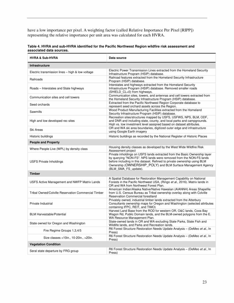
Table 4. HVRA and sub-HVRA identified for the Pacific Northwest Region wildfire risk assessment and
associated data sources........................................................................................................................ 23
Table 5. Flame length values corresponding to Fire Intensity Levels used in assigning response functions.
............................................................................................................................................................ 24
Table 6. Response functions for the Infrastructure HVRA to highlight electric transmission lines. .......... 26
Table 7. Response functions for the Infrastructure HVRA to highlight railroads. ..................................... 27
Table 8. Response functions for the Infrastructure HVRA to highlight interstates and state highways. .... 28
Table 9. Response functions for the Infrastructure HVRA to highlight communication sites and cell
towers. ................................................................................................................................................. 29
Table 10. Response functions for the Infrastructure HVRA to highlight seed orchards. ............................ 30
Table 11. Response functions for the Infrastructure HVRA to highlight sawmills. ................................... 31
Table 12. Response functions for the Infrastructure HVRA to highlight recreation sites. ......................... 33
Table 13. Response functions for the Infrastructure HVRA to highlight ski areas. ................................... 34
Table 14. Response functions for the Infrastructure HVRA to highlight historic structures. ..................... 35
Table 15. Response functions for the People and Property HVRA ............................................................ 37
Table 16. Response functions for the Timber HVRA ................................................................................. 38
Table 17. Response functions for the USFS Timber Sub-HVRA. .............................................................. 39
Table 18. Response functions for the Tribal Timber Sub-HVRA .............................................................. 40
Table 19. Response functions for Private Industrial Timber Sub-HVRA................................................... 41
Table 20. Response functions for BLM Timber Sub-HVRA ..................................................................... 43
Table 21. Response functions for State Timber Sub-HVRA ...................................................................... 44
Table 22. S-Class transition matrix used for the Vegetation Condition HVRA. S-Classes for standard,
five-box BpS models are defined in Table 23. .................................................................................... 46
Table 23. Response function matrix for the standard, five-box BpS models in the Vegetation Condition
HVRA. ................................................................................................................................................ 47
Table 24. Response function matrix for all other BpS models in the Vegetation Condition HVRA. ......... 48
Table 25. Response functions for the Watershed HVRA. .......................................................................... 49
Table 26. Response functions for the Marbled Murrelet Sub-HVRA......................................................... 50
Table 27. Response functions for the Northern Spotted Owl Sub-HVRA.................................................. 51
Table 28. Response functions for Greater Sage-Grouse Sub-HVRA ......................................................... 52
Table 29. Response functions for trout Sub-HVRAs to highlight bull trout............................................... 53
Table 30. Response functions for salmon Sub-HVRAs to highlight chinook salmon. ............................... 54
Table 31. Response functions for salmon Sub-HVRAs to highlight coho salmon. .................................... 55
Table 32. Response functions for trout Sub-HVRAs to highlight steelhead trout. ..................................... 56
Table 33. Response functions for trout Sub-HVRAs to highlight redband trout. ....................................... 57
Table 34. Response functions for trout Sub-HVRAs to highlight coastal cutthroat trout. ......................... 58
Table 35. Response functions for trout Sub-HVRAs to highlight Lahontan cutthroat trout. ...................... 59
Table A1. Zonal summaries of FSim and HVRA data for the 17 national forests within the PNRA
analysis area ........................................................................................................................................ 85
Table A2. Zonal summaries of FSim and HVRA data for a 2-km buffer around the 17 national forests
within the PNRA analysis area. .......................................................................................................... 86
Table A3. Zonal summaries of FSim and HVRA data for each USFS Ranger District within the PNRA
analysis area. ....................................................................................................................................... 87
Table A4. Change log for edits made to this report after the original 1-12-18 release date. ...................... 90
4
List of Figures
Figure 1. Overview of landscape zones for PNRA FSim project. USFS administrative forests are shown in
green, and the Analysis Area (AA) is shown in yellow. The project produces valid BP results within
this AA. To ensure valid BP in the AA, we started fires in the twenty-three numbered fire occurrence
areas (FOAs), outlined in black. To prevent fires from reaching the edge of the fuelscape, a buffered
fuelscape extent was used, which is represented by the blue outline. ................................................... 8
Figure 2. The components of the Quantitative Wildfire Risk Assessment Framework used for PNRA. ..... 9
Figure 3. Map of fuel model groups across the PNRA analysis area.......................................................... 10
Figure 4. Map of the location of edits made to LANDFIRE 2014 (LF_1.4.0) 30-m raster data based on
resource staff input at the fuels review workshop on Nov. 2-3, 2016 in Portland, OR. ..................... 14
Figure 5. Ignition density grid used in FSim simulations. .......................................................................... 16
Figure 6. RAWS stations and ERC sample sites used for the PNRA FSim project. RAWS data were used
for hourly sustained wind speed. ......................................................................................................... 17
Figure 7. Diagram showing the primary elements used to derive Burn Probability. .................................. 20
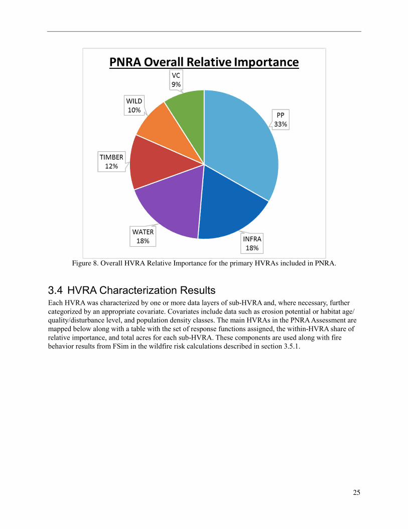
Figure 8. Overall HVRA Relative Importance for the primary HVRAs included in PNRA. ..................... 25
Figure 9. Map of electric transmission lines in the PNRA analysis area .................................................... 26
Figure 10. Map of railroads in the PNRA analysis area ............................................................................. 27
Figure 11. Map of interstates and state highways in the PNRA analysis area. ........................................... 28
Figure 12. Map of all communication and cell tower sites in the PNRA analysis area. ............................. 29
Figure 13. Map of tree seed orchards in the PNRA analysis area. .............................................................. 30
Figure 14. Map of the location of sawmills in the PNRA analysis area. .................................................... 31
Figure 15. Map of high and low developed recreation sites in the PNRA analysis area. ........................... 32
Figure 16. Map of downhill ski area boundaries and infrastructure in the PNRA analysis area. ............... 34
Figure 17. Map of historic structures in the PNRA analysis area. .............................................................. 35
Figure 18. Map of housing density per acre and USFS inholdings in the PNRA analysis area. ................ 36
Figure 19. Map of timber land ownership in the PNRA analysis area........................................................ 38
Figure 20. Map of timber by size class on USFS lands designated as active management within the PNRA
study area ............................................................................................................................................ 39
Figure 21. Map of timber by size class on tribal lands within the PNRA study area. ................................ 40
Figure 22. Map of timber by size class on private industrial lands within the PNRA study area. .............. 41
Figure 23. Map of timber by size class on BLM lands in the PNRA analysis area. ................................... 42
Figure 24. Map of timber by size class on state lands within the PNRA study area................................... 44
Figure 25. Map of FRG used in the Vegetation Condition HVRA within the PNRA analysis area. .......... 45
Figure 26. Map of erosion potential by hazard class within the PNRA analysis area. ............................... 49
Figure 27. Map of marbled murrelet critical habitat in the PNRA analysis area ........................................ 50
Figure 28. Map of predicted northern spotted owl suitable habitat in the PNRA analysis area. ................ 51
Figure 29. Map of greater sage-grouse land use plan allocations in the PNRA analysis area. ................... 52
Figure 30. Map of bull trout distribution in the PNRA analysis area. ........................................................ 53
Figure 31. Map of chinook salmon critical habitat in the PNRA analysis area. ......................................... 54
Figure 32. Map of Oregon coastal coho salmon critical habitat in the PNRA analysis area. ..................... 55
Figure 33. Map of steelhead trout critical habitat in the PNRA analysis area. ........................................... 56
Figure 34. Map of redband trout distribution in the PNRA analysis area. .................................................. 57
Figure 35. Map of coastal cutthroat trout distribution in the PNRA analysis area. .................................... 58
Figure 36. Map of Lahontan trout distribution in the PNRA analysis area. ............................................... 59
Figure 37. Map of integrated FSim burn probability results for the PNRA study area. ............................. 62
Figure 38. Map of FSim flame length exceedance probability: 2-ft. results for the PNRA study area. ..... 63
Figure 39. Map of FSim flame length exceedance probability: 4-ft. results for the PNRA study area. ..... 64
Figure 40. Map of FSim flame length exceedance probability: 6-ft. results for the PNRA study area. ..... 65
Figure 41. Map of FSim flame length exceedance probability: 8-ft. results for the PNRA study area. ..... 66
5
Figure 42. Map illustrating the 2-km buffer area used in the zonal summaries. The 2-km buffer represents
the area between USFS lands and non-USFS lands. The area where two national forests meet is not
included. .............................................................................................................................................. 67
Figure 43. Simulated mean large-fire size and mean number of large fires per million acres per year for
the 17 national forests in the PNRA study area. The curved lines represent lines of equal burn
probability. .......................................................................................................................................... 68
Figure 44. Simulated mean large-fire size and mean number of large fires per million acres per year for a
2-kilometer buffer around the 17 national forests in the PNRA study area. The curved lines represent
lines of equal burn probability. ........................................................................................................... 69
Figure 45. Graph of the 4-foot flame length exceedance probability and burn probability for the 17
national forests in the PNRA study area. ............................................................................................ 70
Figure 46. Graph of the 4-foot flame length exceedance probability and burn probability for a 2-kilometer
buffer around the 17 national forests in the PNRA study area............................................................ 71
Figure 47 . Graph of the 8-foot flame length exceedance probability and burn probability for the 17
national forests in the PNRA study area. ............................................................................................ 72
Figure 48 . Graph of the 8-foot flame length exceedance probability and burn probability for a 2-
kilometer buffer around the 17 national forests in the PNRA study area. .......................................... 73
Figure 49: Weighted net response over all highly valued resources and assets (HVRAs) in the assessment.
HVRAs are listed in order from greatest expected positive net value change (response) at the top, to
greatest negative net value change at the bottom. ............................................................................... 74
Figure 50: Map of Conditional Net Value Change (cNVC) for the PNRA analysis area. .......................... 75
Figure 51: Map of Expected Net Value Change (eNVC) for the PNRA analysis area. .............................. 76
Figure 52. Graph of conditional net value change and burn probability for the 17 national forests in the
PNRA study area. The curved lines represent lines of equal expected net value change. .................. 77
Figure 53. Graph of conditional net value change and burn probability for a 2-kilometer buffer around the
17 national forests in the PNRA study area. The curved lines represent lines of equal expected net
value change. ....................................................................................................................................... 78
6
1 Overview of PNRA
1.1 Purpose of the Assessment
The purpose of the USFS Pacific Northwest Region Wildfire Risk Assessment (PNRA) is to provide
foundational information about wildfire hazard and risk to highly valued resources and assets across the
geographic area. Such information supports wildfires, regional fuel management planning decisions, and
revisions to land and resource management plans. A wildfire risk assessment is a quantitative analysis of
the assets and resources across a specific landscape and how they are potentially impacted by wildfire.
The PNRA analysis considers several different components, each resolved spatially across the region,
including:
• likelihood of a fire burning,
• the intensity of a fire if one should occur,
• the exposure of assets and resources based on their locations, and
• the susceptibility of those assets and resources to wildfire.
Assets are human-made features, such as commercial structures, critical facilities, housing, etc., that have
a specific importance or value. Resources are natural features, such as wildlife habitat, federally
threatened and endangered plant or animal species, etc. These also have a specific importance or value.
Generally, the term “values at risk” has previously been used to describe both assets and resources. For
PNRA, the term Highly Valued Resources and Assets (HVRA) is used to describe what has previously
been labeled values at risk. There are two reasons for this change in terminology. First, resources and
assets are not themselves “values” in any way that term is conventionally defined—they have value
(importance). Second, while resources and assets may be exposed to wildfire, they are not necessarily “at
risk”—that is the purpose of the assessment.
To manage wildfire in the Region, it is essential that accurate wildfire risk data, to the greatest degree
possible, is available to drive fire management strategies. These risk outputs can be used to drive the
planning, prioritization and implementation of prevention and mitigation activities, such as prescribed fire
and mechanical fuel treatments. In addition, the risk data can be used to support fire operations in
response to wildfire incidents by identifying those assets and resources most susceptible to fire. This can
aid in decision making for prioritizing and positioning of firefighting resources.
1.2 Landscape Zones
Analysis Area The Analysis Area (AA) is the area for which valid burn probability (BP) results are produced. The AA
for the Pacific Northwest Region (PNRA) FSim project was initially defined as the Oregon and
Washington state boundaries. All subsequent project boundaries (discussed below) were built from this
initial extent. After wildfire modeling was underway, it was brought to our attention that the AA did not
cover the entire Rogue River-Siskiyou and Wallowa-Whitman National Forests. We later adjusted the AA
to include the state boundaries and the full extent of Region 6 National Forests. The PNRA analysis
includes 17 Administrative Forests: Colville, Deschutes, Fremont-Winema, Gifford Pinchot, Malheur, Mt.
Baker-Snoqualmie, Mt. Hood, Ochoco, Okanogan-Wenatchee, Olympic, Rogue River-Siskiyou, Siuslaw,
7
Umatilla, Umpqua, Wallowa-Whitman, and Willamette National Forests (NF), as well as the Columbia
River Gorge National Scenic Area.
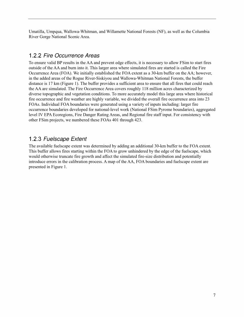
Fire Occurrence Areas To ensure valid BP results in the AA and prevent edge effects, it is necessary to allow FSim to start fires
outside of the AA and burn into it. This larger area where simulated fires are started is called the Fire
Occurrence Area (FOA). We initially established the FOA extent as a 30-km buffer on the AA; however,
in the added areas of the Rogue River-Siskiyou and Wallowa-Whitman National Forests, the buffer
distance is 17 km (Figure 1). The buffer provides a sufficient area to ensure that all fires that could reach
the AA are simulated. The Fire Occurrence Area covers roughly 118 million acres characterized by
diverse topographic and vegetation conditions. To more accurately model this large area where historical
fire occurrence and fire weather are highly variable, we divided the overall fire occurrence area into 23
FOAs. Individual FOA boundaries were generated using a variety of inputs including: larger fire
occurrence boundaries developed for national-level work (National FSim Pyrome boundaries), aggregated
level IV EPA Ecoregions, Fire Danger Rating Areas, and Regional fire staff input. For consistency with
other FSim projects, we numbered these FOAs 401 through 423.
Fuelscape Extent The available fuelscape extent was determined by adding an additional 30-km buffer to the FOA extent.
This buffer allows fires starting within the FOA to grow unhindered by the edge of the fuelscape, which
would otherwise truncate fire growth and affect the simulated fire-size distribution and potentially
introduce errors in the calibration process. A map of the AA, FOA boundaries and fuelscape extent are
presented in Figure 1.
8
Figure 1. Overview of landscape zones for PNRA FSim project. USFS administrative forests are shown in green, and the Analysis Area (AA) is shown in yellow. The project produces valid BP results within this AA. To ensure valid BP in the AA, we started fires in the twenty-three numbered fire occurrence areas (FOAs), outlined in black. To prevent fires from reaching the edge of the fuelscape, a buffered fuelscape extent was used, which is represented by the blue outline.
9
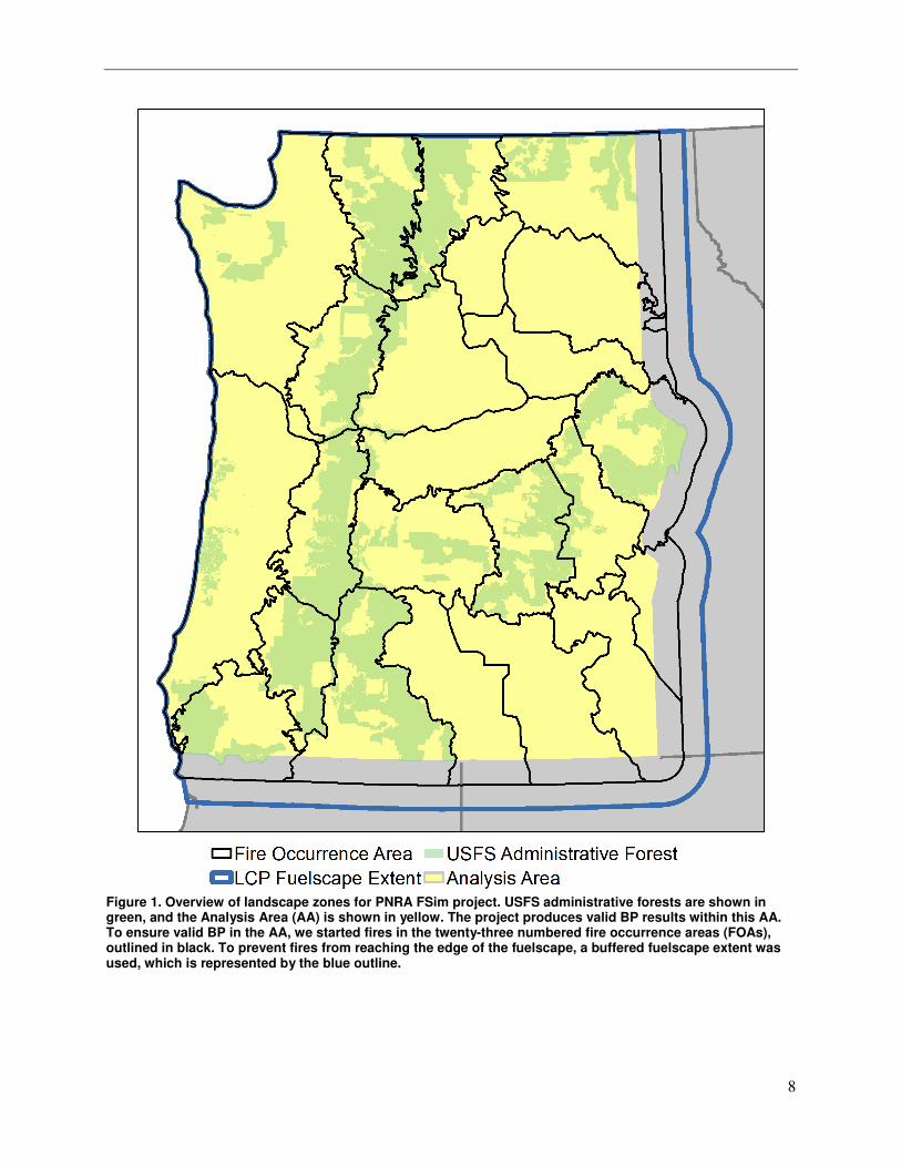
1.3 Quantitative Risk Modeling Framework The basis for a quantitative framework for assessing wildfire risk to highly valued resources and assets
(HVRAs) has been established for many years (Finney, 2005; Scott, 2006). The framework has been
implemented across a variety of scales, from the continental United States (Calkin et al., 2010), to
individual states (Buckley et al., 2014), to a portion of a national forest (Thompson et al., 2013b), to an
individual county. In this framework, wildfire risk is a function of two main factors: 1) wildfire hazard
and 2) HVRA vulnerability (Figure 2).
Wildfire hazard is a physical situation with potential for causing damage to vulnerable resources or
assets. Quantitatively, wildfire hazard is measured by two main factors: 1) burn probability (or likelihood
or burning), and; 2) fire intensity (measured as flame length, fireline intensity, or other similar measure).
For this analysis, we used the large fire simulator (FSim) to quantify wildfire potential across the
landscape at a pixel size of 120 m (approximately 3.5 acres per pixel).
Figure 2. The components of the Quantitative Wildfire Risk Assessment Framework used for PNRA.
HVRA vulnerability is also composed of two factors: 1) exposure and 2) susceptibility. Exposure is the
placement (or coincidental location) of an HVRA in a hazardous environment—for example, building a
home within a flammable landscape. Some HVRAs, like critical wildlife habitat or endangered plants, are
not movable; they are not "placed" in hazardous locations. Still, their exposure to wildfire is the wildfire
hazard where the habitat exists. Finally, the susceptibility of an HVRA to wildfire is how easily it is
damaged by wildfire of different types and intensities. Some assets are fire-hardened and can withstand
very intense fires without damage, whereas others are easily damaged by even low-intensity fire.
2 Analysis Methods and Input Data The FSim large-fire simulator was used to quantify wildfire hazard across the AA at a pixel size of 120 m.
FSim is a comprehensive fire occurrence, growth, behavior, and suppression simulation system that uses
locally relevant fuel, weather, topography, and historical fire occurrence information to make a spatially
resolved estimate of the contemporary likelihood and intensity of wildfire across the landscape (Finney et
al., 2011).
10
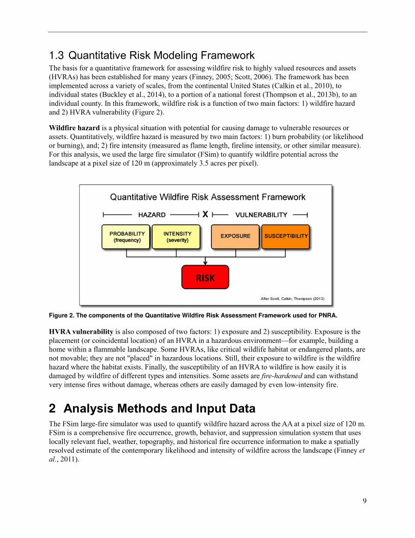
2.1 Fuelscape The fuelscape consists of geospatial data layers representing surface fuel model, canopy base height,
canopy bulk density, canopy cover, canopy height and topography characteristics (slope, aspect,
elevation). The fuelscape was developed from LANDFIRE 2014 (LF_1.4.0) 30-m raster data and was
updated based on resource staff input at the fuels review workshop that took place November 2-3, 2016 in
Portland, OR. Additionally, the fuelscape was updated using Rapid Assessment of Vegetation Condition
after Wildfire (RAVG) and Monitoring Trends in Burn Severity (MTBS) data, along with Northwest
Coordination Center (NWCC) perimeter datasets to account for wildfire disturbances that occurred
between 2015 and 2017. The resulting fuelscape by fuel model group is shown in Figure 3.
Figure 3. Map of fuel model groups across the PNRA analysis area.
11
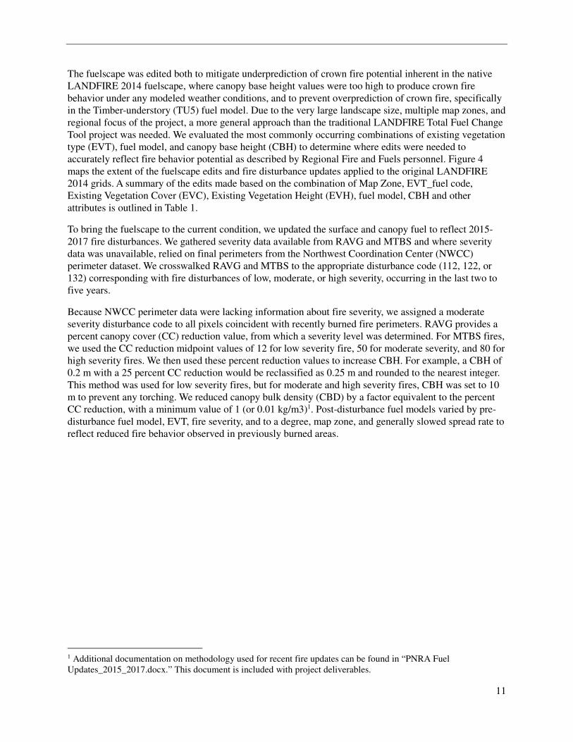
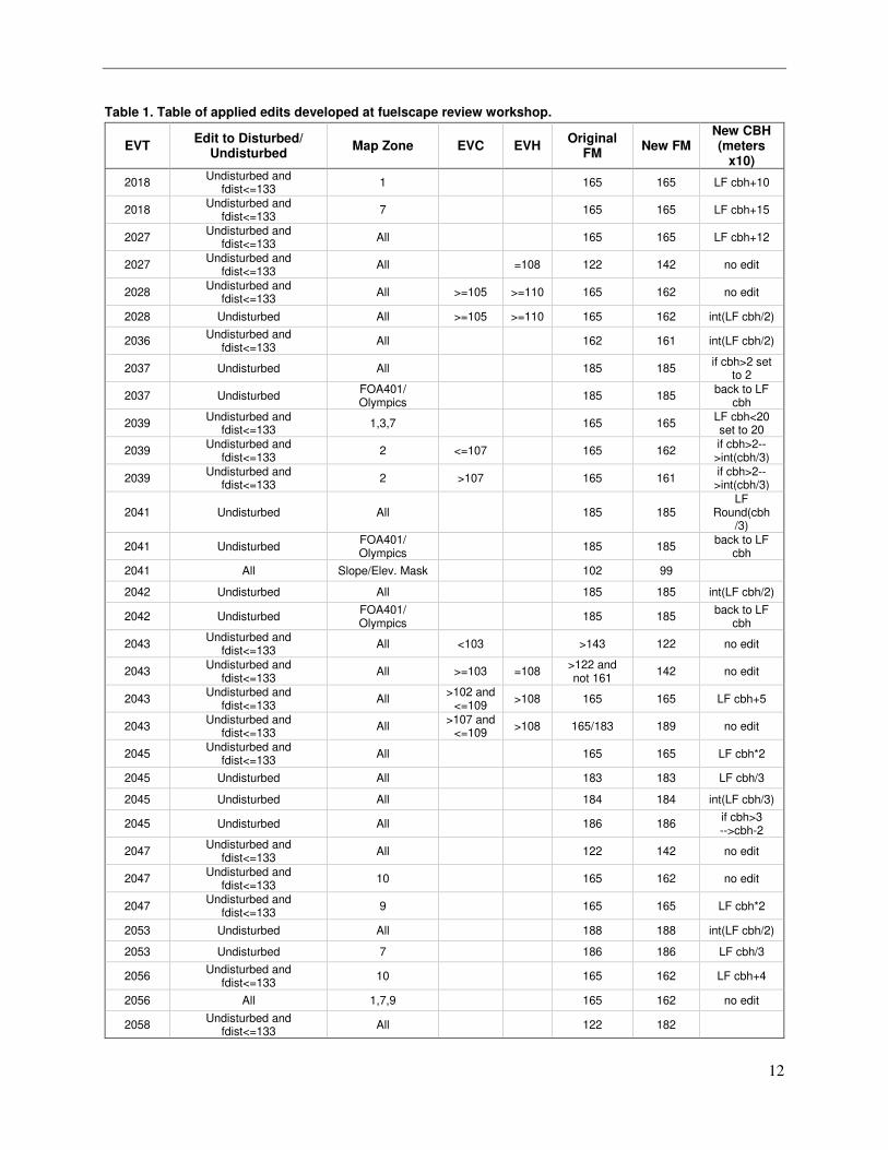
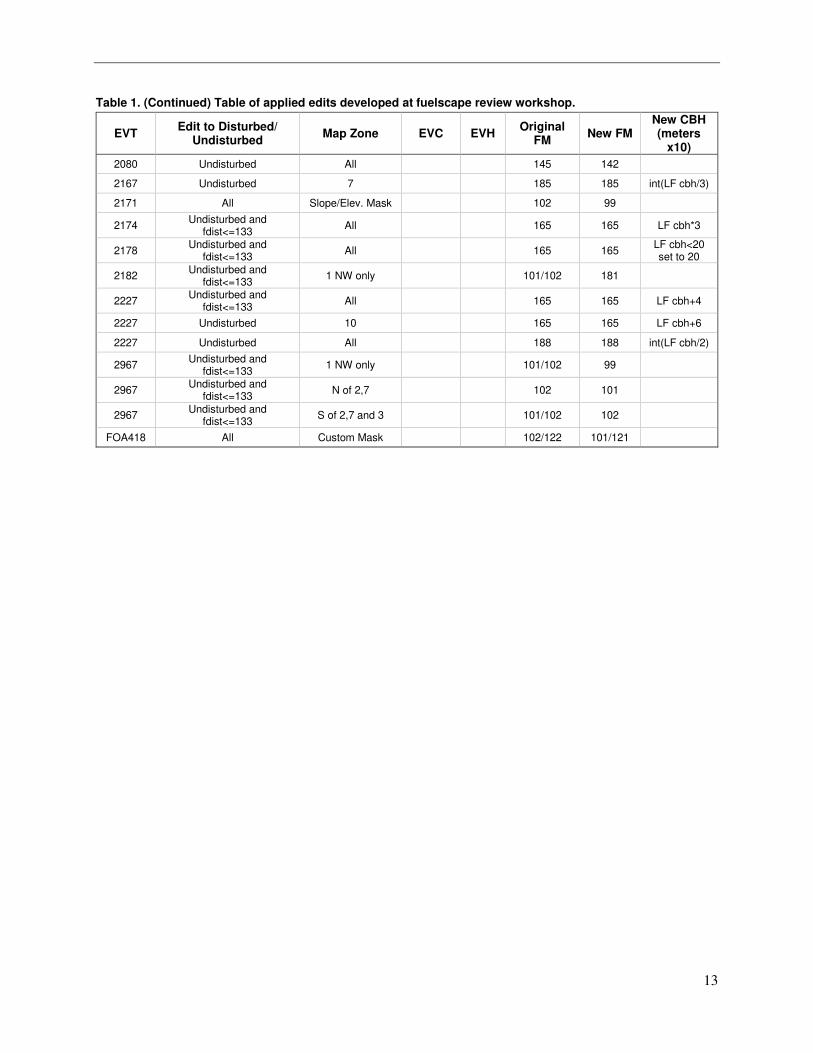
The fuelscape was edited both to mitigate underprediction of crown fire potential inherent in the native
LANDFIRE 2014 fuelscape, where canopy base height values were too high to produce crown fire
behavior under any modeled weather conditions, and to prevent overprediction of crown fire, specifically
in the Timber-understory (TU5) fuel model. Due to the very large landscape size, multiple map zones, and
regional focus of the project, a more general approach than the traditional LANDFIRE Total Fuel Change
Tool project was needed. We evaluated the most commonly occurring combinations of existing vegetation
type (EVT), fuel model, and canopy base height (CBH) to determine where edits were needed to
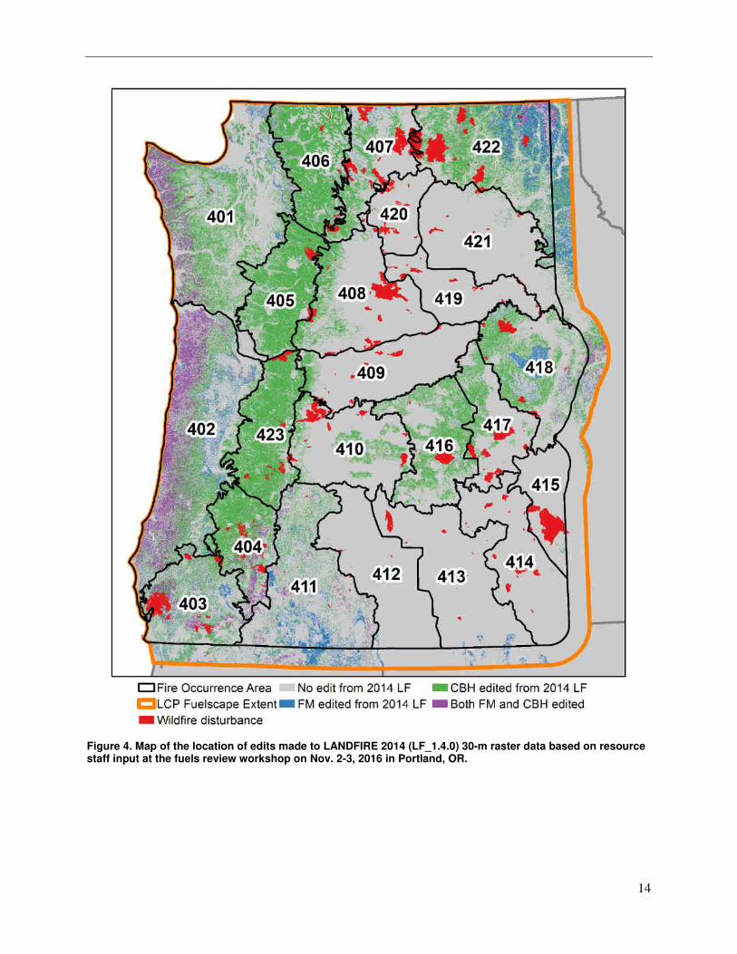
accurately reflect fire behavior potential as described by Regional Fire and Fuels personnel. Figure 4
maps the extent of the fuelscape edits and fire disturbance updates applied to the original LANDFIRE
2014 grids. A summary of the edits made based on the combination of Map Zone, EVT_fuel code,
Existing Vegetation Cover (EVC), Existing Vegetation Height (EVH), fuel model, CBH and other
attributes is outlined in Table 1.
To bring the fuelscape to the current condition, we updated the surface and canopy fuel to reflect 2015-
2017 fire disturbances. We gathered severity data available from RAVG and MTBS and where severity
data was unavailable, relied on final perimeters from the Northwest Coordination Center (NWCC)
perimeter dataset. We crosswalked RAVG and MTBS to the appropriate disturbance code (112, 122, or
132) corresponding with fire disturbances of low, moderate, or high severity, occurring in the last two to
five years.
Because NWCC perimeter data were lacking information about fire severity, we assigned a moderate
severity disturbance code to all pixels coincident with recently burned fire perimeters. RAVG provides a
percent canopy cover (CC) reduction value, from which a severity level was determined. For MTBS fires,
we used the CC reduction midpoint values of 12 for low severity fire, 50 for moderate severity, and 80 for
high severity fires. We then used these percent reduction values to increase CBH. For example, a CBH of
0.2 m with a 25 percent CC reduction would be reclassified as 0.25 m and rounded to the nearest integer.
This method was used for low severity fires, but for moderate and high severity fires, CBH was set to 10
m to prevent any torching. We reduced canopy bulk density (CBD) by a factor equivalent to the percent
CC reduction, with a minimum value of 1 (or 0.01 kg/m3)1. Post-disturbance fuel models varied by pre-
disturbance fuel model, EVT, fire severity, and to a degree, map zone, and generally slowed spread rate to
reflect reduced fire behavior observed in previously burned areas.
1 Additional documentation on methodology used for recent fire updates can be found in “PNRA Fuel
Updates_2015_2017.docx.” This document is included with project deliverables.
12
Table 1. Table of applied edits developed at fuelscape review workshop.
EVT Edit to Disturbed/
Undisturbed Map Zone EVC EVH
Original FM
New FM New CBH (meters
x10)
2018 Undisturbed and
fdist<=133 1 165 165 LF cbh+10
2018 Undisturbed and
fdist<=133 7 165 165 LF cbh+15
2027 Undisturbed and
fdist<=133 All 165 165 LF cbh+12
2027 Undisturbed and
fdist<=133 All =108 122 142 no edit
2028 Undisturbed and
fdist<=133 All >=105 >=110 165 162 no edit
2028 Undisturbed All >=105 >=110 165 162 int(LF cbh/2)
2036 Undisturbed and
fdist<=133 All 162 161 int(LF cbh/2)
2037 Undisturbed All 185 185 if cbh>2 set
to 2
2037 Undisturbed FOA401/ Olympics
185 185 back to LF
cbh
2039 Undisturbed and
fdist<=133 1,3,7 165 165
LF cbh<20 set to 20
2039 Undisturbed and
fdist<=133 2 <=107 165 162
if cbh>2-->int(cbh/3)
2039 Undisturbed and
fdist<=133 2 >107 165 161
if cbh>2-->int(cbh/3)
2041 Undisturbed All 185 185 LF
Round(cbh /3)
2041 Undisturbed FOA401/ Olympics
185 185 back to LF
cbh
2041 All Slope/Elev. Mask 102 99
2042 Undisturbed All 185 185 int(LF cbh/2)
2042 Undisturbed FOA401/ Olympics
185 185 back to LF
cbh
2043 Undisturbed and
fdist<=133 All <103 >143 122 no edit
2043 Undisturbed and
fdist<=133 All >=103 =108
>122 and not 161
142 no edit
2043 Undisturbed and
fdist<=133 All
>102 and <=109
>108 165 165 LF cbh+5
2043 Undisturbed and
fdist<=133 All
>107 and <=109
>108 165/183 189 no edit
2045 Undisturbed and
fdist<=133 All 165 165 LF cbh*2
2045 Undisturbed All 183 183 LF cbh/3
2045 Undisturbed All 184 184 int(LF cbh/3)
2045 Undisturbed All 186 186 if cbh>3 -->cbh-2
2047 Undisturbed and
fdist<=133 All 122 142 no edit
2047 Undisturbed and
fdist<=133 10 165 162 no edit
2047 Undisturbed and
fdist<=133 9 165 165 LF cbh*2
2053 Undisturbed All 188 188 int(LF cbh/2)
2053 Undisturbed 7 186 186 LF cbh/3
2056 Undisturbed and
fdist<=133 10 165 162 LF cbh+4
2056 All 1,7,9 165 162 no edit
2058 Undisturbed and
fdist<=133 All 122 182
13
Table 1. (Continued) Table of applied edits developed at fuelscape review workshop.
EVT Edit to Disturbed/
Undisturbed Map Zone EVC EVH
Original FM
New FM
New CBH (meters
x10)
2080 Undisturbed All 145 142
2167 Undisturbed 7 185 185 int(LF cbh/3)
2171 All Slope/Elev. Mask 102 99
2174 Undisturbed and
fdist<=133 All 165 165 LF cbh*3
2178 Undisturbed and
fdist<=133 All 165 165
LF cbh<20 set to 20
2182 Undisturbed and
fdist<=133 1 NW only 101/102 181
2227 Undisturbed and
fdist<=133 All 165 165 LF cbh+4
2227 Undisturbed 10 165 165 LF cbh+6
2227 Undisturbed All 188 188 int(LF cbh/2)
2967 Undisturbed and
fdist<=133 1 NW only 101/102 99
2967 Undisturbed and
fdist<=133 N of 2,7 102 101
2967 Undisturbed and
fdist<=133 S of 2,7 and 3 101/102 102
FOA418 All Custom Mask 102/122 101/121
14
Figure 4. Map of the location of edits made to LANDFIRE 2014 (LF_1.4.0) 30-m raster data based on resource staff input at the fuels review workshop on Nov. 2-3, 2016 in Portland, OR.
15
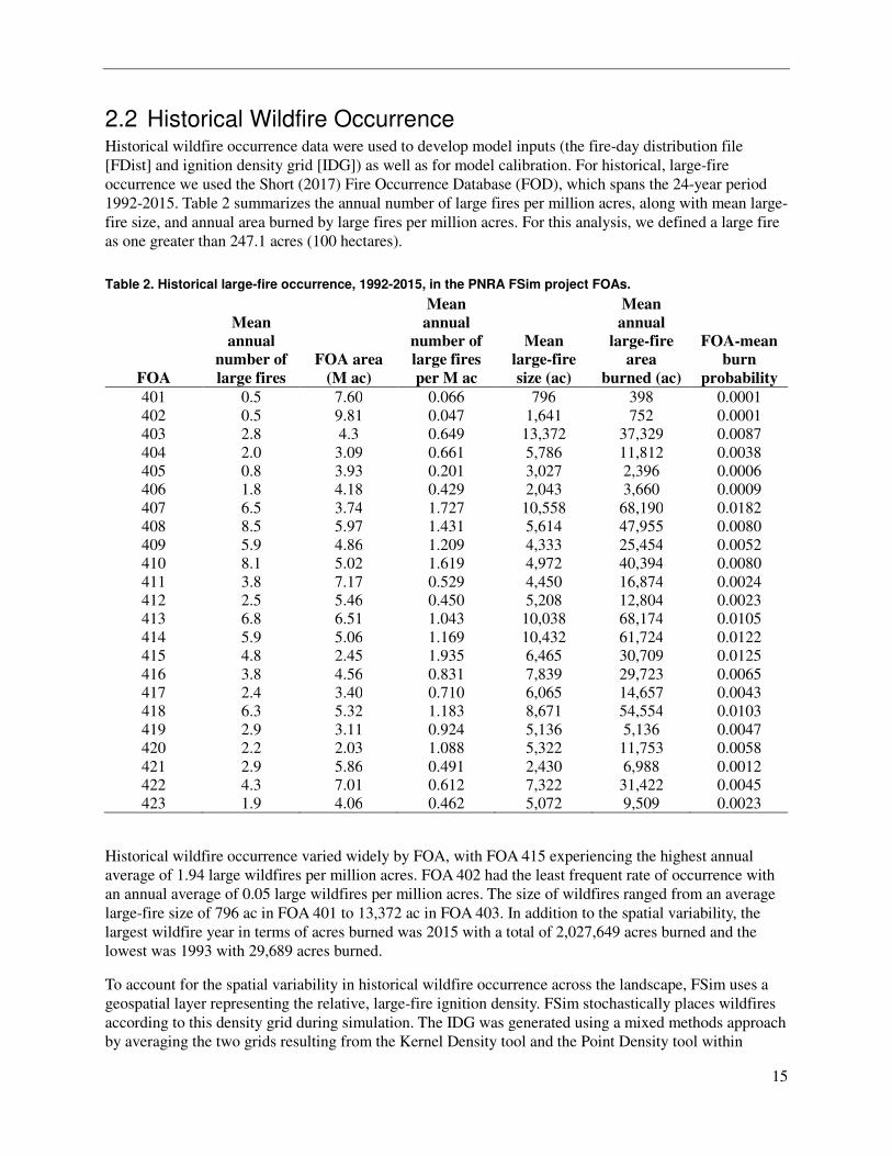
2.2 Historical Wildfire Occurrence Historical wildfire occurrence data were used to develop model inputs (the fire-day distribution file
[FDist] and ignition density grid [IDG]) as well as for model calibration. For historical, large-fire
occurrence we used the Short (2017) Fire Occurrence Database (FOD), which spans the 24-year period
1992-2015. Table 2 summarizes the annual number of large fires per million acres, along with mean large-
fire size, and annual area burned by large fires per million acres. For this analysis, we defined a large fire
as one greater than 247.1 acres (100 hectares).
Table 2. Historical large-fire occurrence, 1992-2015, in the PNRA FSim project FOAs.
FOA
Mean
annual
number of
large fires
FOA area
(M ac)
Mean
annual
number of
large fires
per M ac
Mean
large-fire
size (ac)
Mean
annual
large-fire
area
burned (ac)
FOA-mean
burn
probability
401 0.5 7.60 0.066 796 398 0.0001
402 0.5 9.81 0.047 1,641 752 0.0001
403 2.8 4.3 0.649 13,372 37,329 0.0087
404 2.0 3.09 0.661 5,786 11,812 0.0038
405 0.8 3.93 0.201 3,027 2,396 0.0006
406 1.8 4.18 0.429 2,043 3,660 0.0009
407 6.5 3.74 1.727 10,558 68,190 0.0182
408 8.5 5.97 1.431 5,614 47,955 0.0080
409 5.9 4.86 1.209 4,333 25,454 0.0052
410 8.1 5.02 1.619 4,972 40,394 0.0080
411 3.8 7.17 0.529 4,450 16,874 0.0024
412 2.5 5.46 0.450 5,208 12,804 0.0023
413 6.8 6.51 1.043 10,038 68,174 0.0105
414 5.9 5.06 1.169 10,432 61,724 0.0122
415 4.8 2.45 1.935 6,465 30,709 0.0125
416 3.8 4.56 0.831 7,839 29,723 0.0065
417 2.4 3.40 0.710 6,065 14,657 0.0043
418 6.3 5.32 1.183 8,671 54,554 0.0103
419 2.9 3.11 0.924 5,136 5,136 0.0047
420 2.2 2.03 1.088 5,322 11,753 0.0058
421 2.9 5.86 0.491 2,430 6,988 0.0012
422 4.3 7.01 0.612 7,322 31,422 0.0045
423 1.9 4.06 0.462 5,072 9,509 0.0023
Historical wildfire occurrence varied widely by FOA, with FOA 415 experiencing the highest annual
average of 1.94 large wildfires per million acres. FOA 402 had the least frequent rate of occurrence with
an annual average of 0.05 large wildfires per million acres. The size of wildfires ranged from an average
large-fire size of 796 ac in FOA 401 to 13,372 ac in FOA 403. In addition to the spatial variability, the
largest wildfire year in terms of acres burned was 2015 with a total of 2,027,649 acres burned and the
lowest was 1993 with 29,689 acres burned.
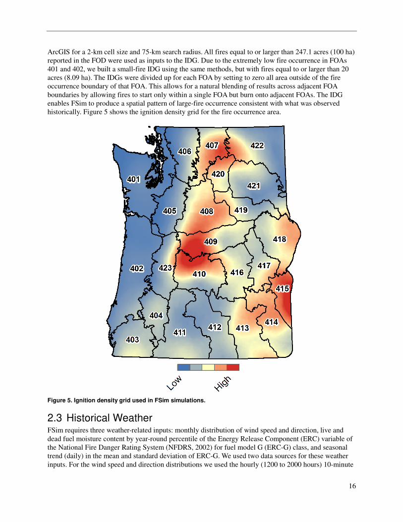
To account for the spatial variability in historical wildfire occurrence across the landscape, FSim uses a
geospatial layer representing the relative, large-fire ignition density. FSim stochastically places wildfires
according to this density grid during simulation. The IDG was generated using a mixed methods approach
by averaging the two grids resulting from the Kernel Density tool and the Point Density tool within
16
ArcGIS for a 2-km cell size and 75-km search radius. All fires equal to or larger than 247.1 acres (100 ha)
reported in the FOD were used as inputs to the IDG. Due to the extremely low fire occurrence in FOAs
401 and 402, we built a small-fire IDG using the same methods, but with fires equal to or larger than 20
acres (8.09 ha). The IDGs were divided up for each FOA by setting to zero all area outside of the fire
occurrence boundary of that FOA. This allows for a natural blending of results across adjacent FOA
boundaries by allowing fires to start only within a single FOA but burn onto adjacent FOAs. The IDG
enables FSim to produce a spatial pattern of large-fire occurrence consistent with what was observed
historically. Figure 5 shows the ignition density grid for the fire occurrence area.
Figure 5. Ignition density grid used in FSim simulations.
2.3 Historical Weather FSim requires three weather-related inputs: monthly distribution of wind speed and direction, live and
dead fuel moisture content by year-round percentile of the Energy Release Component (ERC) variable of
the National Fire Danger Rating System (NFDRS, 2002) for fuel model G (ERC-G) class, and seasonal
trend (daily) in the mean and standard deviation of ERC-G. We used two data sources for these weather
inputs. For the wind speed and direction distributions we used the hourly (1200 to 2000 hours) 10-minute
17
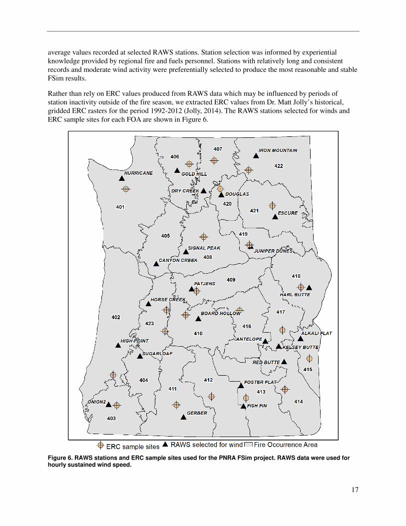
average values recorded at selected RAWS stations. Station selection was informed by experiential
knowledge provided by regional fire and fuels personnel. Stations with relatively long and consistent
records and moderate wind activity were preferentially selected to produce the most reasonable and stable
FSim results.
Rather than rely on ERC values produced from RAWS data which may be influenced by periods of
station inactivity outside of the fire season, we extracted ERC values from Dr. Matt Jolly’s historical,
gridded ERC rasters for the period 1992-2012 (Jolly, 2014). The RAWS stations selected for winds and
ERC sample sites for each FOA are shown in Figure 6.
Figure 6. RAWS stations and ERC sample sites used for the PNRA FSim project. RAWS data were used for hourly sustained wind speed.
18
Fire-day Distribution File (FDist) Fire-day Distribution files are used by FSim to generate stochastic fire ignitions as a function of ERC.
The FDist files were generated using an R script that summarizes historical ERC and wildfire occurrence
data, performs logistic regression, and then formats the results into the required FDist format.
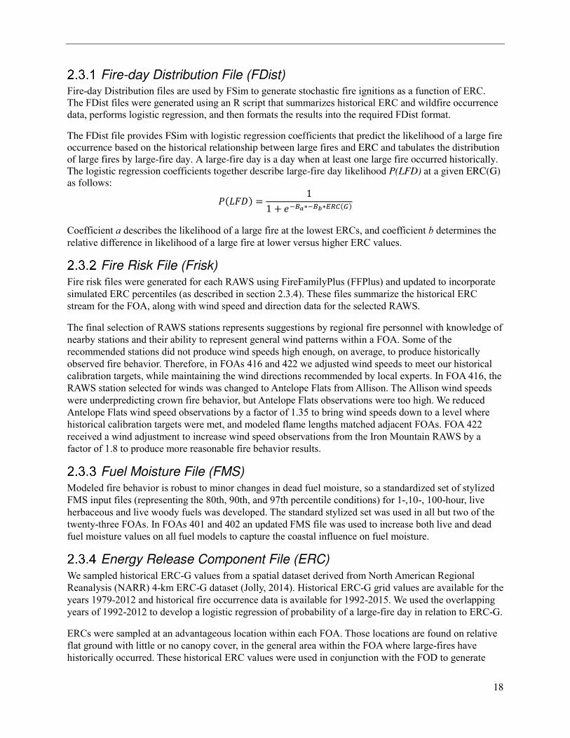
The FDist file provides FSim with logistic regression coefficients that predict the likelihood of a large fire
occurrence based on the historical relationship between large fires and ERC and tabulates the distribution
of large fires by large-fire day. A large-fire day is a day when at least one large fire occurred historically.
The logistic regression coefficients together describe large-fire day likelihood P(LFD) at a given ERC(G)
as follows:
������ � 11 �� ∗���∗������
Coefficient a describes the likelihood of a large fire at the lowest ERCs, and coefficient b determines the
relative difference in likelihood of a large fire at lower versus higher ERC values.
Fire Risk File (Frisk) Fire risk files were generated for each RAWS using FireFamilyPlus (FFPlus) and updated to incorporate
simulated ERC percentiles (as described in section 2.3.4). These files summarize the historical ERC
stream for the FOA, along with wind speed and direction data for the selected RAWS.
The final selection of RAWS stations represents suggestions by regional fire personnel with knowledge of
nearby stations and their ability to represent general wind patterns within a FOA. Some of the
recommended stations did not produce wind speeds high enough, on average, to produce historically
observed fire behavior. Therefore, in FOAs 416 and 422 we adjusted wind speeds to meet our historical
calibration targets, while maintaining the wind directions recommended by local experts. In FOA 416, the
RAWS station selected for winds was changed to Antelope Flats from Allison. The Allison wind speeds
were underpredicting crown fire behavior, but Antelope Flats observations were too high. We reduced
Antelope Flats wind speed observations by a factor of 1.35 to bring wind speeds down to a level where
historical calibration targets were met, and modeled flame lengths matched adjacent FOAs. FOA 422
received a wind adjustment to increase wind speed observations from the Iron Mountain RAWS by a
factor of 1.8 to produce more reasonable fire behavior results.
Fuel Moisture File (FMS) Modeled fire behavior is robust to minor changes in dead fuel moisture, so a standardized set of stylized
FMS input files (representing the 80th, 90th, and 97th percentile conditions) for 1-,10-, 100-hour, live
herbaceous and live woody fuels was developed. The standard stylized set was used in all but two of the
twenty-three FOAs. In FOAs 401 and 402 an updated FMS file was used to increase both live and dead
fuel moisture values on all fuel models to capture the coastal influence on fuel moisture.
Energy Release Component File (ERC) We sampled historical ERC-G values from a spatial dataset derived from North American Regional
Reanalysis (NARR) 4-km ERC-G dataset (Jolly, 2014). Historical ERC-G grid values are available for the
years 1979-2012 and historical fire occurrence data is available for 1992-2015. We used the overlapping
years of 1992-2012 to develop a logistic regression of probability of a large-fire day in relation to ERC-G.
ERCs were sampled at an advantageous location within each FOA. Those locations are found on relative
flat ground with little or no canopy cover, in the general area within the FOA where large-fires have
historically occurred. These historical ERC values were used in conjunction with the FOD to generate
19
FSim’s FDist input file, but not for the Frisk file. ERC percentile information in the Frisk file was
generated from the simulated ERC stream, described below. This approach ensures consistency between
the simulated and historical ERCs.
For simulated ERCs in FSim, we used a new feature of FSim that allows the user to supply a stream of
ERC values for each FOA. Isaac Grenfell, statistician at the Missoula Fire Sciences Lab, has generated
1,000 years of daily ERC values (365,000 ERC values) on the same 4-km grid as Jolly’s historical ERCs.
The simulated ERC values Grenfell produces are “coordinated” in that a given year and day for one FOA
corresponds to the same year and day in all other FOAs—their values only differ due to their location on
the landscape. This coordination permits analysis of fire-year information across all FOAs.
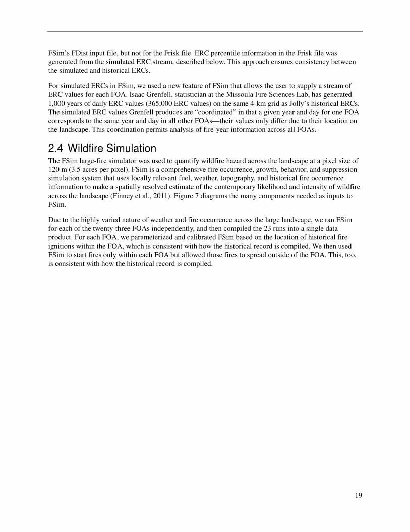
2.4 Wildfire Simulation The FSim large-fire simulator was used to quantify wildfire hazard across the landscape at a pixel size of
120 m (3.5 acres per pixel). FSim is a comprehensive fire occurrence, growth, behavior, and suppression
simulation system that uses locally relevant fuel, weather, topography, and historical fire occurrence
information to make a spatially resolved estimate of the contemporary likelihood and intensity of wildfire
across the landscape (Finney et al., 2011). Figure 7 diagrams the many components needed as inputs to
FSim.
Due to the highly varied nature of weather and fire occurrence across the large landscape, we ran FSim
for each of the twenty-three FOAs independently, and then compiled the 23 runs into a single data
product. For each FOA, we parameterized and calibrated FSim based on the location of historical fire
ignitions within the FOA, which is consistent with how the historical record is compiled. We then used
FSim to start fires only within each FOA but allowed those fires to spread outside of the FOA. This, too,
is consistent with how the historical record is compiled.
20
Figure 7. Diagram showing the primary elements used to derive Burn Probability.
Model Calibration FSim simulations for each FOA were calibrated to historical measures of large fire occurrence including:
mean historical large-fire size, mean annual burn probability, mean annual number of large fires per
million acres, and mean annual area burned per million acres. From these measures, two calculations are
particularly useful for comparing against and adjusting FSim results: 1) mean large fire size, and 2)
number of large fires per million acres.
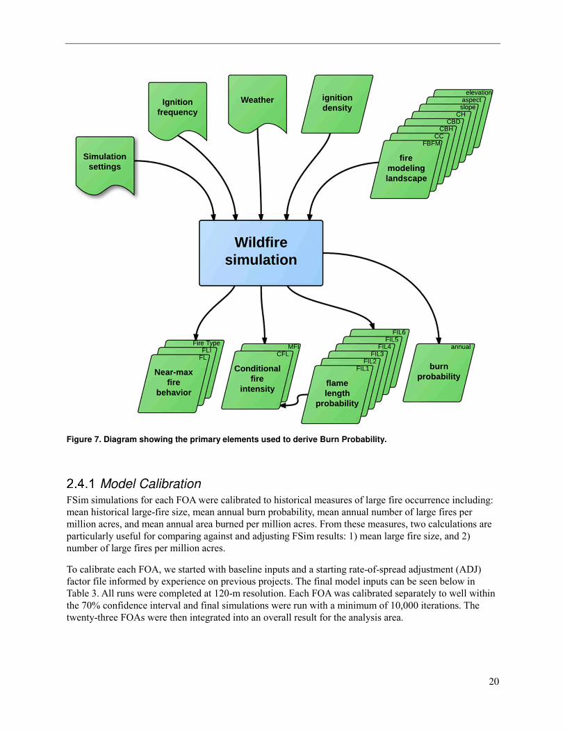
To calibrate each FOA, we started with baseline inputs and a starting rate-of-spread adjustment (ADJ)
factor file informed by experience on previous projects. The final model inputs can be seen below in
Table 3. All runs were completed at 120-m resolution. Each FOA was calibrated separately to well within
the 70% confidence interval and final simulations were run with a minimum of 10,000 iterations. The
twenty-three FOAs were then integrated into an overall result for the analysis area.
21
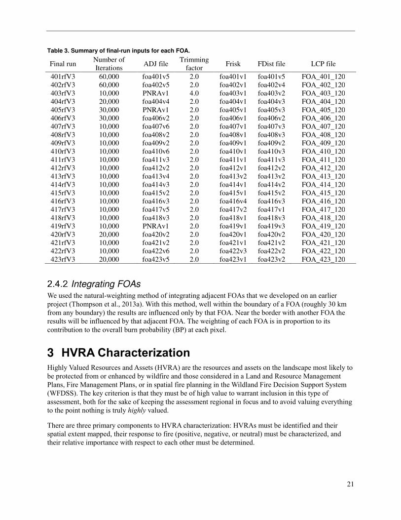
Table 3. Summary of final-run inputs for each FOA.
Final run Number of
Iterations ADJ file
Trimming
factor Frisk FDist file LCP file
401rfV3 60,000 foa401v5 2.0 foa401v1 foa401v5 FOA_401_120
402rfV3 60,000 foa402v5 2.0 foa402v1 foa402v4 FOA_402_120
403rfV3 10,000 PNRAv1 4.0 foa403v1 foa403v2 FOA_403_120
404rfV3 20,000 foa404v4 2.0 foa404v1 foa404v3 FOA_404_120
405rfV3 30,000 PNRAv1 2.0 foa405v1 foa405v3 FOA_405_120
406rfV3 30,000 foa406v2 2.0 foa406v1 foa406v2 FOA_406_120
407rfV3 10,000 foa407v6 2.0 foa407v1 foa407v3 FOA_407_120
408rfV3 10,000 foa408v2 2.0 foa408v1 foa408v3 FOA_408_120
409rfV3 10,000 foa409v2 2.0 foa409v1 foa409v2 FOA_409_120
410rfV3 10,000 foa410v6 2.0 foa410v1 foa410v3 FOA_410_120
411rfV3 10,000 foa411v3 2.0 foa411v1 foa411v3 FOA_411_120
412rfV3 10,000 foa412v2 2.0 foa412v1 foa412v2 FOA_412_120
413rfV3 10,000 foa413v4 2.0 foa413v2 foa413v2 FOA_413_120
414rfV3 10,000 foa414v3 2.0 foa414v1 foa414v2 FOA_414_120
415rfV3 10,000 foa415v2 2.0 foa415v1 foa415v2 FOA_415_120
416rfV3 10,000 foa416v3 2.0 foa416v4 foa416v3 FOA_416_120
417rfV3 10,000 foa417v5 2.0 foa417v2 foa417v1 FOA_417_120
418rfV3 10,000 foa418v3 2.0 foa418v1 foa418v3 FOA_418_120
419rfV3 10,000 PNRAv1 2.0 foa419v1 foa419v3 FOA_419_120
420rfV3 20,000 foa420v2 2.0 foa420v1 foa420v2 FOA_420_120
421rfV3 10,000 foa421v2 2.0 foa421v1 foa421v2 FOA_421_120
422rfV3 10,000 foa422v6 2.0 foa422v3 foa422v2 FOA_422_120
423rfV3 20,000 foa423v5 2.0 foa423v1 foa423v2 FOA_423_120
Integrating FOAs We used the natural-weighting method of integrating adjacent FOAs that we developed on an earlier
project (Thompson et al., 2013a). With this method, well within the boundary of a FOA (roughly 30 km
from any boundary) the results are influenced only by that FOA. Near the border with another FOA the
results will be influenced by that adjacent FOA. The weighting of each FOA is in proportion to its
contribution to the overall burn probability (BP) at each pixel.
3 HVRA Characterization Highly Valued Resources and Assets (HVRA) are the resources and assets on the landscape most likely to
be protected from or enhanced by wildfire and those considered in a Land and Resource Management
Plans, Fire Management Plans, or in spatial fire planning in the Wildland Fire Decision Support System
(WFDSS). The key criterion is that they must be of high value to warrant inclusion in this type of
assessment, both for the sake of keeping the assessment regional in focus and to avoid valuing everything
to the point nothing is truly highly valued.
There are three primary components to HVRA characterization: HVRAs must be identified and their
spatial extent mapped, their response to fire (positive, negative, or neutral) must be characterized, and
their relative importance with respect to each other must be determined.
22
3.1 HVRA Identification A set of HVRA was identified through a workshop held at the Pacific Northwest Region Regional Office
(SORO) on November 4, 2016. A group consisting of Fire/Fuels Planners, Resource Specialists, Wildlife
Biologists, Geospatial Analysts, and representatives from Oregon Department of Forestry (ODF) and
Washington Department of Natural Resources (DNR) identified six HVRAs in total: two assets and four
resources. The complete list of HVRAs and their associated data sources are listed in Table 4.
To the degree possible, HVRAs are mapped to the extent of the Analysis Area boundary (Figure 1). This
is the boundary used to summarize the final risk results. Some HVRA are limited to the Forest boundary,
due to the nature of the data (e.g., extracted from Regional corporate databases for FS land only).
3.2 Response Functions Each HVRA selected for the assessment must also have an associated response to fire, whether it is
positive or negative. We relied on input from Regional Resource Specialists, the Fuels Program Staff,
along with Nature Conservancy, BLM, and DNR representatives at a workshop held February 28-March
1, 2017 at the Regional Office. In these workshops, the group discussed how each resource or asset
responded to fires of different intensity levels and characterized the HVRA response using values ranging
from -100 to +100. The flame length values corresponding to the fire intensity levels reported by FSim
are shown in Table 5. The response functions (RFs) used in the risk results are shown in Table 6 through
Table 35 below.
3.3 Relative Importance The relative importance (RI) assignments are needed to integrate results across all HVRAs. Without this
input from leadership, all HVRAs would be weighted equally. The RI workshop was held at SORO on
May 16, 2017 and was attended by Line Officers or representatives from the states of Oregon and
Washington; BLM Field, District or State Office; and Forest Service Ranger District, Forest, or Regional
Office. The focus of this workshop was to establish the importance and ranking of the primary HVRAs
relative to each other. The People and Property HVRA received the greatest share of RI at 33 percent,
followed by the Municipal Watersheds and Infrastructure HVRAs, each receiving 18 percent of the total
importance. Timber was allocated 12 percent and Wildlife received 10 percent. Finally, Vegetation
Condition received 9 percent of the total landscape importance (Figure 8). These importance percentages
reflect the importance per unit area of all mapped HVRA.
Sub-HVRA relative importance was determined by the Regional Fire Planner and Resource Specialists.
Sub-RIs are based on both the relative importance per unit area and mapped extent of the Sub-HVRA
layers within the primary HVRA category. In Table 6 through Table 35, we provide the share of HVRA
relative importance within the primary HVRA.
Relative importance values were generally developed by first ranking the Sub-HVRAs then assigning an
RI value to each. The most important Sub-HVRA was assigned RI = 100. Each remaining Sub-HVRA
was then assigned an RI value indicating its importance relative to that most important Sub-HVRA.
The RI values apply to the overall HVRA on the assessment landscape as a whole. The calculations need
to account for the relative extent of each HVRA to avoid overemphasizing HVRAs that cover many acres.
This was accomplished by normalizing the calculations by the relative extent (RE) of each HVRA in the
assessment area. Here, relative extent refers to the number of 30-m pixels mapped to each HVRA. In
using this method, the relative importance of each HVRA is spread out over the HVRA's extent. An
HVRA with few pixels can have a high importance per pixel; and an HVRA with a great many pixels can
23
have a low importance per pixel. A weighting factor (called Relative Importance Per Pixel [RIPP])
representing the relative importance per unit area was calculated for each HVRA.
Table 4. HVRA and sub-HVRA identified for the Pacific Northwest Region wildfire risk assessment and associated data sources.
HVRA & Sub-HVRA Data source
Infrastructure
Electric transmission lines – high & low voltage Electric Power Transmission Lines extracted from the Homeland Security Infrastructure Program (HSIP) database.
Railroads Railroad features extracted from the Homeland Security Infrastructure Program (HSIP) database.
Roads – Interstates and State highways Interstates and highways extracted from the Homeland Security Infrastructure Program (HSIP) database. Removed smaller roads (SHIELD_CL=0) from highways.
Communication sites and cell towers Communication sites, towers, and antennas and cell towers extracted from the Homeland Security Infrastructure Program (HSIP) database.
Seed orchards Extracted from the Pacific Northwest Region Corporate database to represent seed orchard assets across the Region.
Sawmills Wood Product Manufacturing Facilities extracted from the Homeland Security Infrastructure Program (HSIP) database.
High and low developed rec sites Recreation sites/structures mapped by USFS, USFWS, NPS, BLM, ODF, and DNR and including state, county, and local parks and campgrounds. High vs. low investment level assigned based on dataset attributes.
Ski Areas OR and WA ski area boundaries, digitized outer edge and infrastructure using Google Earth imagery
Historic buildings Historic buildings as recorded by the National Register of Historic Places
People and Property
Where People Live (WPL) by density class Housing density classes as developed by the West Wide Wildfire Risk Assessment project
USFS Private Inholdings
Private inholdings on USFS lands extracted from the Basic Ownership layer by querying "NON-FS". NPS lands were removed from the NON-FS lands before including in this dataset. Refined to private ownership using BLM
Ownership (OWNERSHIP_POLY) and BLM Surface Management Agency (BLM_SMA_FS_update).
Timber
USFS Active Management and NWFP Matrix Lands A Spatial Database for Restoration Management Capability on National Forests in the Pacific Northwest USA, (Ringo et al., 2016). Matrix lands in OR and WA from Northwest Forest Plan.
Tribal Owned/Colville Reservation Commercial Timber American Indian/Alaska Native/Native Hawaiian (AIANNH) Areas Shapefile from U.S. Census Bureau as Tribal ownership overlay along with Colville Reservation Commercial forestland
Private Industrial Privately owned, industrial timber lands extracted from the Atterbury Consultants ownership maps for Oregon and Washington (selected attributes containing IFPC, REIT, and TIMO)
BLM Harvestable/Potential Harvest Land Base from the ROD for western OR, O&C lands, Coos Bay Wagon Rd, Public Domain lands, and the BLM-owned polygons from the E. WA Resource Management Plan.
State owned for Oregon and Washington State-owned lands in OR and WA excluding State Parks, State Fish and Wildlife lands, and Parks and Recreation lands.
Fire Regime Groups 1,3,4/5 R6 Forest Structure Restoration Needs Update Analysis – (DeMeo et al., In Press)
Size classes <10in., 10-20in., >20in. R6 Forest Structure Restoration Needs Update Analysis – (DeMeo et al., In Press)
Vegetation Condition
Seral state departure by FRG group R6 Forest Structure Restoration Needs Update Analysis – (DeMeo et al., In Press)
24
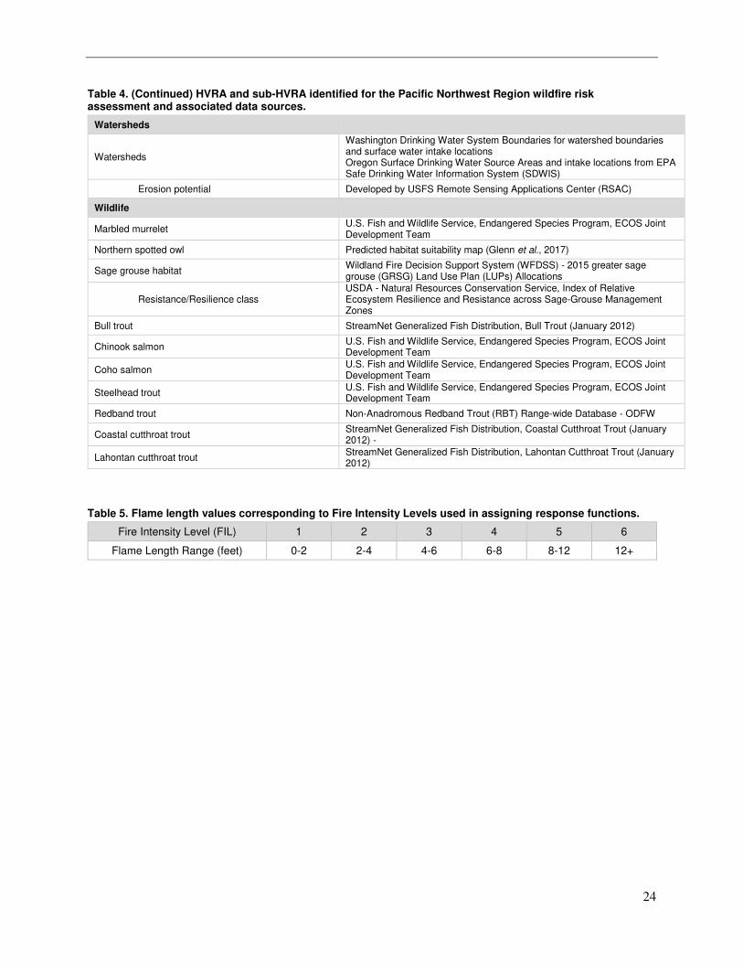
Table 4. (Continued) HVRA and sub-HVRA identified for the Pacific Northwest Region wildfire risk assessment and associated data sources.
Watersheds
Watersheds
Washington Drinking Water System Boundaries for watershed boundaries and surface water intake locations Oregon Surface Drinking Water Source Areas and intake locations from EPA Safe Drinking Water Information System (SDWIS)
Erosion potential Developed by USFS Remote Sensing Applications Center (RSAC)
Wildlife
Marbled murrelet U.S. Fish and Wildlife Service, Endangered Species Program, ECOS Joint Development Team
Northern spotted owl Predicted habitat suitability map (Glenn et al., 2017)
Sage grouse habitat Wildland Fire Decision Support System (WFDSS) - 2015 greater sage grouse (GRSG) Land Use Plan (LUPs) Allocations
Resistance/Resilience class USDA - Natural Resources Conservation Service, Index of Relative Ecosystem Resilience and Resistance across Sage-Grouse Management Zones
Bull trout StreamNet Generalized Fish Distribution, Bull Trout (January 2012)
Chinook salmon U.S. Fish and Wildlife Service, Endangered Species Program, ECOS Joint Development Team
Coho salmon U.S. Fish and Wildlife Service, Endangered Species Program, ECOS Joint Development Team
Steelhead trout U.S. Fish and Wildlife Service, Endangered Species Program, ECOS Joint Development Team
Redband trout Non-Anadromous Redband Trout (RBT) Range-wide Database - ODFW
Coastal cutthroat trout StreamNet Generalized Fish Distribution, Coastal Cutthroat Trout (January 2012) -
Lahontan cutthroat trout StreamNet Generalized Fish Distribution, Lahontan Cutthroat Trout (January 2012)
Table 5. Flame length values corresponding to Fire Intensity Levels used in assigning response functions.
Fire Intensity Level (FIL) 1 2 3 4 5 6
Flame Length Range (feet) 0-2 2-4 4-6 6-8 8-12 12+
25
Figure 8. Overall HVRA Relative Importance for the primary HVRAs included in PNRA.
3.4 HVRA Characterization Results Each HVRA was characterized by one or more data layers of sub-HVRA and, where necessary, further
categorized by an appropriate covariate. Covariates include data such as erosion potential or habitat age/
quality/disturbance level, and population density classes. The main HVRAs in the PNRA Assessment are
mapped below along with a table with the set of response functions assigned, the within-HVRA share of
relative importance, and total acres for each sub-HVRA. These components are used along with fire
behavior results from FSim in the wildfire risk calculations described in section 3.5.1.
26
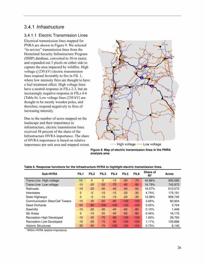
Infrastructure
Electric Transmission Lines
Electrical transmission lines mapped for
PNRA are shown in Figure 9. We selected
“in service” transmission lines from the
Homeland Security Infrastructure Program
(HSIP) database, converted to 30-m raster,
and expanded out 3 pixels on either side to
capture the area impacted by wildfire. High
voltage (≥230 kV) electric transmission
lines respond favorably to fire in FIL 1,
where low intensity fires are thought to have
a fuel treatment effect. High voltage lines
have a neutral response in FILs 2-3, but an
increasingly negative response in FILs 4-6
(Table 6). Low voltage lines (230 kV) are
thought to be mostly wooden poles, and
therefore, respond negatively to fires of
increasing intensity.
Due to the number of acres mapped on the
landscape and their importance to
infrastructure, electric transmission lines
received 58 percent of the share of the
Infrastructure HVRA importance. The share
of HVRA importance is based on relative
importance per unit area and mapped extent.
Figure 9. Map of electric transmission lines in the PNRA analysis area
Table 6. Response functions for the Infrastructure HVRA to highlight electric transmission lines.
Sub-HVRA FIL1 FIL2 FIL3 FIL4 FIL5 FIL6 Share of
RI1 Acres
Trans-Line- High voltage 10 0 0 -10 -50 -70 40.86% 905,585
Trans-Line- Low voltage -10 -20 -50 -70 -80 -90 16.79% 743,972
Railroads -10 -20 -30 -40 -50 -50 16.57% 612,073
Interstates 0 -5 -10 -15 -20 -30 4.74% 175,191
State Highways 0 -5 -10 -15 -20 -30 12.98% 958,745
Communication Sites/Cell Towers -10 -30 -60 -80 -100 -100 3.65% 80,924
Seed Orchards -50 -90 -100 -100 -100 -100 0.02% 2,704
Sawmills -10 -20 -30 -40 -60 -80 0.10% 1,448
Ski Areas 0 -10 -20 -40 -60 -80 0.44% 16,175
Recreation High Developed -10 -30 -70 -90 -100 -100 1.93% 26,793
Recreation Low Developed -10 -30 -70 -90 -100 -100 1.17% 129,886
Historic Structures -30 -50 -70 -100 -100 -100 0.73% 8,140 1 Within-HVRA relative importance.
27
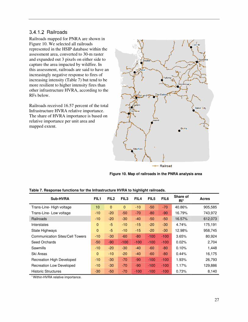
Railroads
Railroads mapped for PNRA are shown in
Figure 10. We selected all railroads
represented in the HSIP database within the
assessment area, converted to 30-m raster
and expanded out 3 pixels on either side to
capture the area impacted by wildfire. In
this assessment, railroads are said to have an
increasingly negative response to fires of
increasing intensity (Table 7) but tend to be
more resilient to higher intensity fires than
other infrastructure HVRA, according to the
RFs below.
Railroads received 16.57 percent of the total
Infrastructure HVRA relative importance.
The share of HVRA importance is based on
relative importance per unit area and
mapped extent.
Figure 10. Map of railroads in the PNRA analysis area
Table 7. Response functions for the Infrastructure HVRA to highlight railroads.
Sub-HVRA FIL1 FIL2 FIL3 FIL4 FIL5 FIL6 Share of
RI1 Acres
Trans-Line- High voltage 10 0 0 -10 -50 -70 40.86% 905,585
Trans-Line- Low voltage -10 -20 -50 -70 -80 -90 16.79% 743,972
Railroads -10 -20 -30 -40 -50 -50 16.57% 612,073
Interstates 0 -5 -10 -15 -20 -30 4.74% 175,191
State Highways 0 -5 -10 -15 -20 -30 12.98% 958,745
Communication Sites/Cell Towers -10 -30 -60 -80 -100 -100 3.65% 80,924
Seed Orchards -50 -90 -100 -100 -100 -100 0.02% 2,704
Sawmills -10 -20 -30 -40 -60 -80 0.10% 1,448
Ski Areas 0 -10 -20 -40 -60 -80 0.44% 16,175
Recreation High Developed -10 -30 -70 -90 -100 -100 1.93% 26,793
Recreation Low Developed -10 -30 -70 -90 -100 -100 1.17% 129,886
Historic Structures -30 -50 -70 -100 -100 -100 0.73% 8,140
1 Within-HVRA relative importance.
28
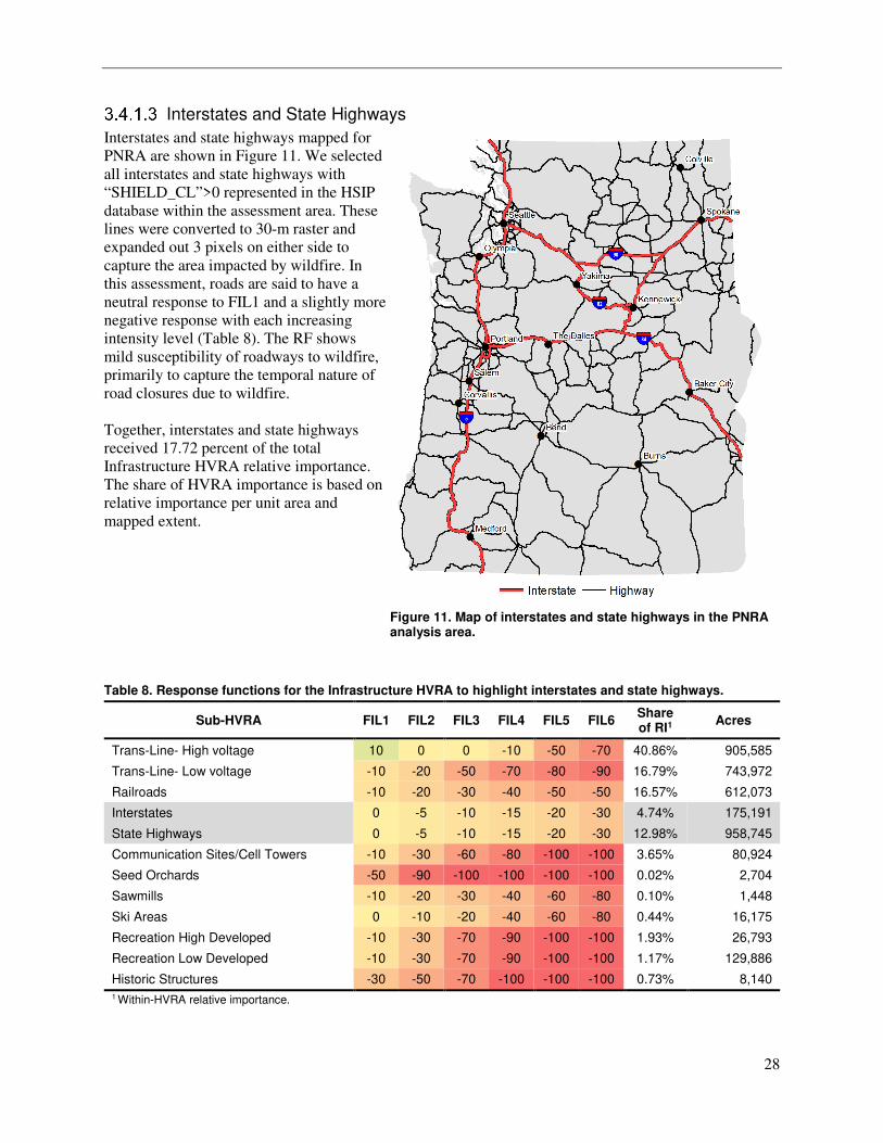
Interstates and State Highways
Interstates and state highways mapped for
PNRA are shown in Figure 11. We selected
all interstates and state highways with
“SHIELD_CL”>0 represented in the HSIP
database within the assessment area. These
lines were converted to 30-m raster and
expanded out 3 pixels on either side to
capture the area impacted by wildfire. In
this assessment, roads are said to have a
neutral response to FIL1 and a slightly more
negative response with each increasing
intensity level (Table 8). The RF shows
mild susceptibility of roadways to wildfire,
primarily to capture the temporal nature of
road closures due to wildfire.
Together, interstates and state highways
received 17.72 percent of the total
Infrastructure HVRA relative importance.
The share of HVRA importance is based on
relative importance per unit area and
mapped extent.
Figure 11. Map of interstates and state highways in the PNRA analysis area.
Table 8. Response functions for the Infrastructure HVRA to highlight interstates and state highways.
Sub-HVRA FIL1 FIL2 FIL3 FIL4 FIL5 FIL6 Share of RI1
Acres
Trans-Line- High voltage 10 0 0 -10 -50 -70 40.86% 905,585
Trans-Line- Low voltage -10 -20 -50 -70 -80 -90 16.79% 743,972
Railroads -10 -20 -30 -40 -50 -50 16.57% 612,073
Interstates 0 -5 -10 -15 -20 -30 4.74% 175,191
State Highways 0 -5 -10 -15 -20 -30 12.98% 958,745
Communication Sites/Cell Towers -10 -30 -60 -80 -100 -100 3.65% 80,924
Seed Orchards -50 -90 -100 -100 -100 -100 0.02% 2,704
Sawmills -10 -20 -30 -40 -60 -80 0.10% 1,448
Ski Areas 0 -10 -20 -40 -60 -80 0.44% 16,175
Recreation High Developed -10 -30 -70 -90 -100 -100 1.93% 26,793
Recreation Low Developed -10 -30 -70 -90 -100 -100 1.17% 129,886
Historic Structures -30 -50 -70 -100 -100 -100 0.73% 8,140 1 Within-HVRA relative importance.
29
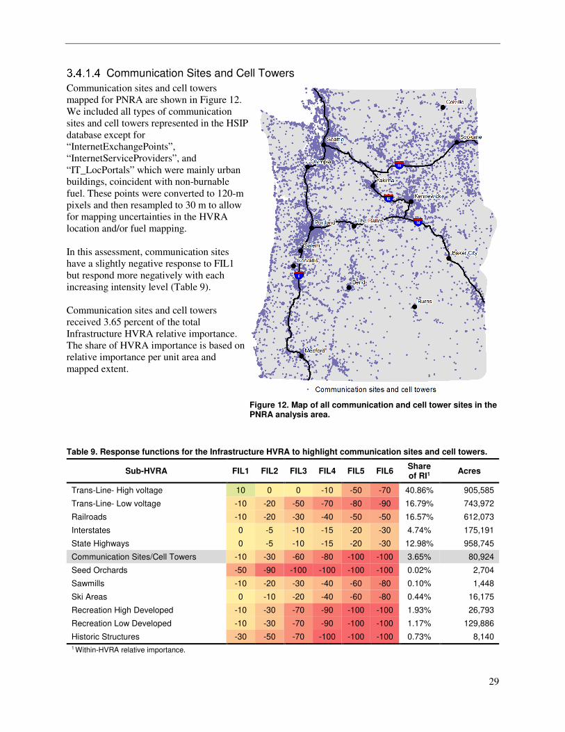
Communication Sites and Cell Towers
Communication sites and cell towers
mapped for PNRA are shown in Figure 12.
We included all types of communication
sites and cell towers represented in the HSIP
database except for
“InternetExchangePoints”,
“InternetServiceProviders”, and
“IT_LocPortals” which were mainly urban
buildings, coincident with non-burnable
fuel. These points were converted to 120-m
pixels and then resampled to 30 m to allow
for mapping uncertainties in the HVRA
location and/or fuel mapping.
In this assessment, communication sites
have a slightly negative response to FIL1
but respond more negatively with each
increasing intensity level (Table 9).
Communication sites and cell towers
received 3.65 percent of the total
Infrastructure HVRA relative importance.
The share of HVRA importance is based on
relative importance per unit area and
mapped extent.
Figure 12. Map of all communication and cell tower sites in the PNRA analysis area.
Table 9. Response functions for the Infrastructure HVRA to highlight communication sites and cell towers.
Sub-HVRA FIL1 FIL2 FIL3 FIL4 FIL5 FIL6 Share of RI1
Acres
Trans-Line- High voltage 10 0 0 -10 -50 -70 40.86% 905,585
Trans-Line- Low voltage -10 -20 -50 -70 -80 -90 16.79% 743,972
Railroads -10 -20 -30 -40 -50 -50 16.57% 612,073
Interstates 0 -5 -10 -15 -20 -30 4.74% 175,191
State Highways 0 -5 -10 -15 -20 -30 12.98% 958,745
Communication Sites/Cell Towers -10 -30 -60 -80 -100 -100 3.65% 80,924
Seed Orchards -50 -90 -100 -100 -100 -100 0.02% 2,704
Sawmills -10 -20 -30 -40 -60 -80 0.10% 1,448
Ski Areas 0 -10 -20 -40 -60 -80 0.44% 16,175
Recreation High Developed -10 -30 -70 -90 -100 -100 1.93% 26,793
Recreation Low Developed -10 -30 -70 -90 -100 -100 1.17% 129,886
Historic Structures -30 -50 -70 -100 -100 -100 0.73% 8,140 1 Within-HVRA relative importance.
30
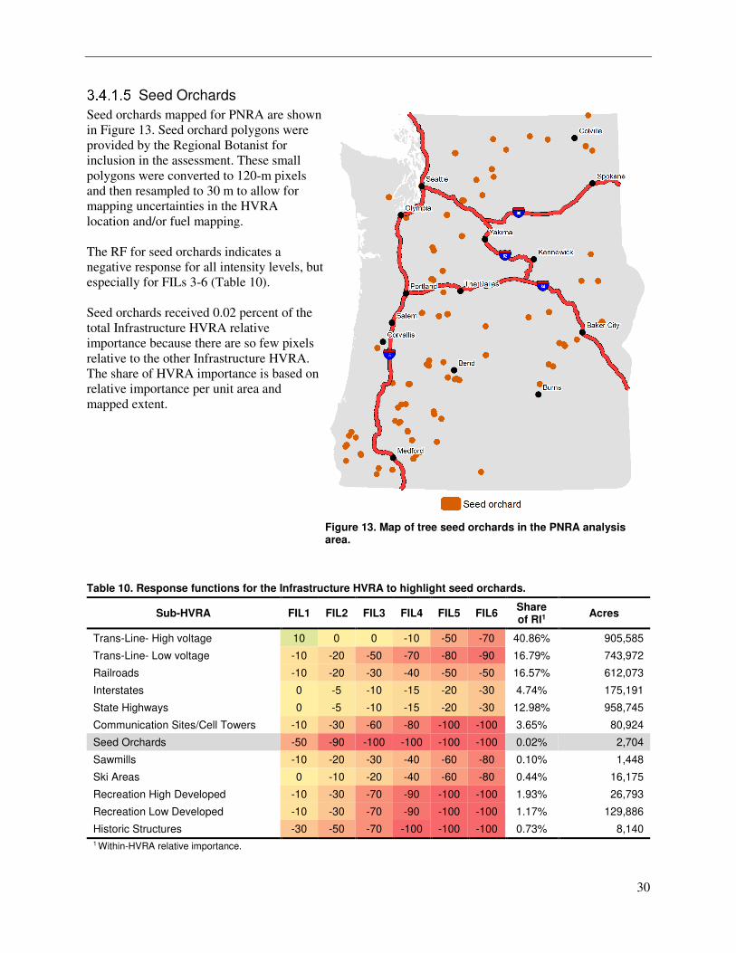
Seed Orchards
Seed orchards mapped for PNRA are shown
in Figure 13. Seed orchard polygons were
provided by the Regional Botanist for
inclusion in the assessment. These small
polygons were converted to 120-m pixels
and then resampled to 30 m to allow for
mapping uncertainties in the HVRA
location and/or fuel mapping.
The RF for seed orchards indicates a
negative response for all intensity levels, but
especially for FILs 3-6 (Table 10).
Seed orchards received 0.02 percent of the
total Infrastructure HVRA relative
importance because there are so few pixels
relative to the other Infrastructure HVRA.
The share of HVRA importance is based on
relative importance per unit area and
mapped extent.
Figure 13. Map of tree seed orchards in the PNRA analysis area.
Table 10. Response functions for the Infrastructure HVRA to highlight seed orchards.
Sub-HVRA FIL1 FIL2 FIL3 FIL4 FIL5 FIL6 Share of RI1
Acres
Trans-Line- High voltage 10 0 0 -10 -50 -70 40.86% 905,585
Trans-Line- Low voltage -10 -20 -50 -70 -80 -90 16.79% 743,972
Railroads -10 -20 -30 -40 -50 -50 16.57% 612,073
Interstates 0 -5 -10 -15 -20 -30 4.74% 175,191
State Highways 0 -5 -10 -15 -20 -30 12.98% 958,745
Communication Sites/Cell Towers -10 -30 -60 -80 -100 -100 3.65% 80,924
Seed Orchards -50 -90 -100 -100 -100 -100 0.02% 2,704
Sawmills -10 -20 -30 -40 -60 -80 0.10% 1,448
Ski Areas 0 -10 -20 -40 -60 -80 0.44% 16,175
Recreation High Developed -10 -30 -70 -90 -100 -100 1.93% 26,793
Recreation Low Developed -10 -30 -70 -90 -100 -100 1.17% 129,886
Historic Structures -30 -50 -70 -100 -100 -100 0.73% 8,140 1 Within-HVRA relative importance.
31
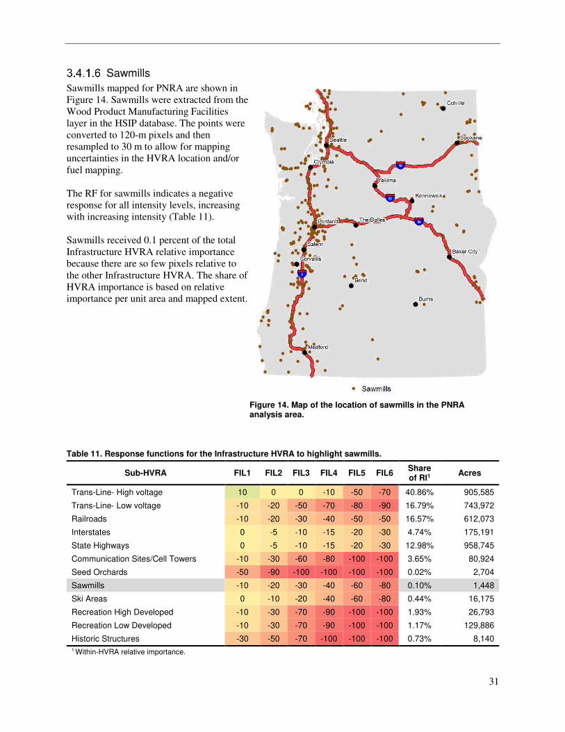
Sawmills
Sawmills mapped for PNRA are shown in
Figure 14. Sawmills were extracted from the
Wood Product Manufacturing Facilities
layer in the HSIP database. The points were
converted to 120-m pixels and then
resampled to 30 m to allow for mapping
uncertainties in the HVRA location and/or
fuel mapping.
The RF for sawmills indicates a negative
response for all intensity levels, increasing
with increasing intensity (Table 11).
Sawmills received 0.1 percent of the total
Infrastructure HVRA relative importance
because there are so few pixels relative to
the other Infrastructure HVRA. The share of
HVRA importance is based on relative
importance per unit area and mapped extent.
Figure 14. Map of the location of sawmills in the PNRA analysis area.
Table 11. Response functions for the Infrastructure HVRA to highlight sawmills.
Sub-HVRA FIL1 FIL2 FIL3 FIL4 FIL5 FIL6 Share of RI1
Acres
Trans-Line- High voltage 10 0 0 -10 -50 -70 40.86% 905,585
Trans-Line- Low voltage -10 -20 -50 -70 -80 -90 16.79% 743,972
Railroads -10 -20 -30 -40 -50 -50 16.57% 612,073
Interstates 0 -5 -10 -15 -20 -30 4.74% 175,191
State Highways 0 -5 -10 -15 -20 -30 12.98% 958,745
Communication Sites/Cell Towers -10 -30 -60 -80 -100 -100 3.65% 80,924
Seed Orchards -50 -90 -100 -100 -100 -100 0.02% 2,704
Sawmills -10 -20 -30 -40 -60 -80 0.10% 1,448
Ski Areas 0 -10 -20 -40 -60 -80 0.44% 16,175
Recreation High Developed -10 -30 -70 -90 -100 -100 1.93% 26,793
Recreation Low Developed -10 -30 -70 -90 -100 -100 1.17% 129,886
Historic Structures -30 -50 -70 -100 -100 -100 0.73% 8,140 1 Within-HVRA relative importance.
32
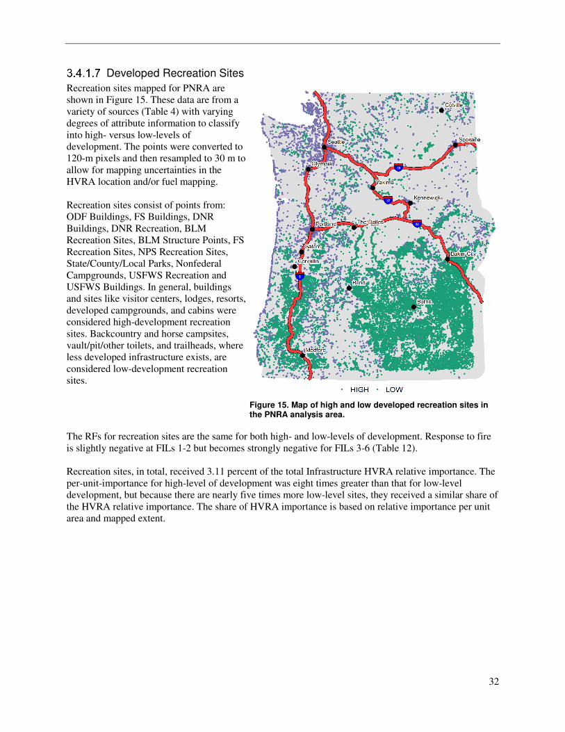
Developed Recreation Sites
Recreation sites mapped for PNRA are
shown in Figure 15. These data are from a
variety of sources (Table 4) with varying
degrees of attribute information to classify
into high- versus low-levels of
development. The points were converted to
120-m pixels and then resampled to 30 m to
allow for mapping uncertainties in the
HVRA location and/or fuel mapping.
Recreation sites consist of points from:
ODF Buildings, FS Buildings, DNR
Buildings, DNR Recreation, BLM
Recreation Sites, BLM Structure Points, FS
Recreation Sites, NPS Recreation Sites,
State/County/Local Parks, Nonfederal
Campgrounds, USFWS Recreation and
USFWS Buildings. In general, buildings
and sites like visitor centers, lodges, resorts,
developed campgrounds, and cabins were
considered high-development recreation
sites. Backcountry and horse campsites,
vault/pit/other toilets, and trailheads, where
less developed infrastructure exists, are
considered low-development recreation
sites.
Figure 15. Map of high and low developed recreation sites in the PNRA analysis area.
The RFs for recreation sites are the same for both high- and low-levels of development. Response to fire
is slightly negative at FILs 1-2 but becomes strongly negative for FILs 3-6 (Table 12).
Recreation sites, in total, received 3.11 percent of the total Infrastructure HVRA relative importance. The
per-unit-importance for high-level of development was eight times greater than that for low-level
development, but because there are nearly five times more low-level sites, they received a similar share of
the HVRA relative importance. The share of HVRA importance is based on relative importance per unit
area and mapped extent.
33
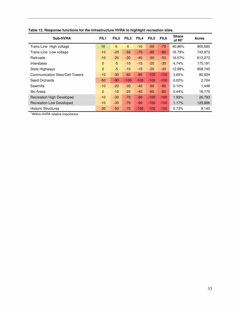
Table 12. Response functions for the Infrastructure HVRA to highlight recreation sites.
Sub-HVRA FIL1 FIL2 FIL3 FIL4 FIL5 FIL6 Share of RI1
Acres
Trans-Line- High voltage 10 0 0 -10 -50 -70 40.86% 905,585
Trans-Line- Low voltage -10 -20 -50 -70 -80 -90 16.79% 743,972
Railroads -10 -20 -30 -40 -50 -50 16.57% 612,073
Interstates 0 -5 -10 -15 -20 -30 4.74% 175,191
State Highways 0 -5 -10 -15 -20 -30 12.98% 958,745
Communication Sites/Cell Towers -10 -30 -60 -80 -100 -100 3.65% 80,924
Seed Orchards -50 -90 -100 -100 -100 -100 0.02% 2,704
Sawmills -10 -20 -30 -40 -60 -80 0.10% 1,448
Ski Areas 0 -10 -20 -40 -60 -80 0.44% 16,175
Recreation High Developed -10 -30 -70 -90 -100 -100 1.93% 26,793
Recreation Low Developed -10 -30 -70 -90 -100 -100 1.17% 129,886
Historic Structures -30 -50 -70 -100 -100 -100 0.73% 8,140 1 Within-HVRA relative importance.
34
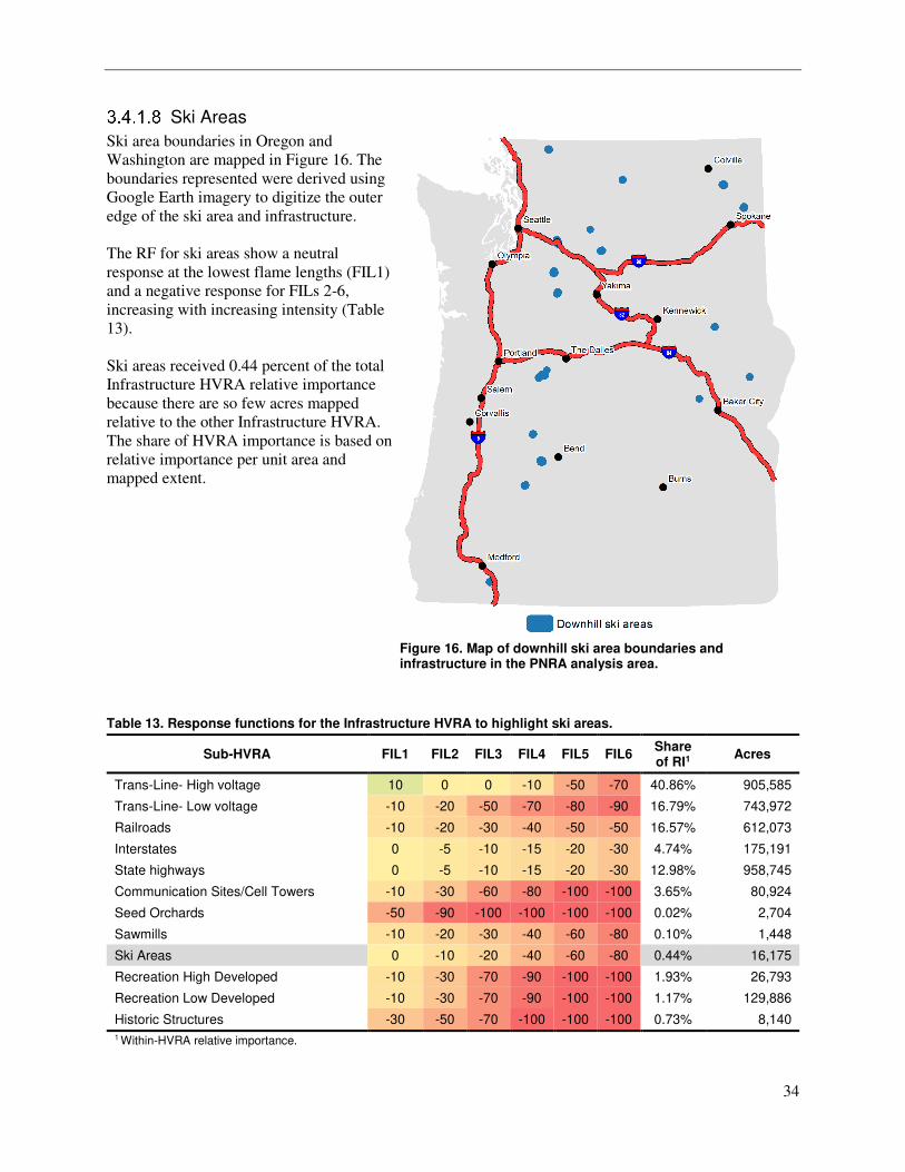
Ski Areas
Ski area boundaries in Oregon and
Washington are mapped in Figure 16. The
boundaries represented were derived using
Google Earth imagery to digitize the outer
edge of the ski area and infrastructure.
The RF for ski areas show a neutral
response at the lowest flame lengths (FIL1)
and a negative response for FILs 2-6,
increasing with increasing intensity (Table
13).
Ski areas received 0.44 percent of the total
Infrastructure HVRA relative importance
because there are so few acres mapped
relative to the other Infrastructure HVRA.
The share of HVRA importance is based on
relative importance per unit area and
mapped extent.
Figure 16. Map of downhill ski area boundaries and infrastructure in the PNRA analysis area.
Table 13. Response functions for the Infrastructure HVRA to highlight ski areas.
Sub-HVRA FIL1 FIL2 FIL3 FIL4 FIL5 FIL6 Share of RI1
Acres
Trans-Line- High voltage 10 0 0 -10 -50 -70 40.86% 905,585
Trans-Line- Low voltage -10 -20 -50 -70 -80 -90 16.79% 743,972
Railroads -10 -20 -30 -40 -50 -50 16.57% 612,073
Interstates 0 -5 -10 -15 -20 -30 4.74% 175,191
State highways 0 -5 -10 -15 -20 -30 12.98% 958,745
Communication Sites/Cell Towers -10 -30 -60 -80 -100 -100 3.65% 80,924
Seed Orchards -50 -90 -100 -100 -100 -100 0.02% 2,704
Sawmills -10 -20 -30 -40 -60 -80 0.10% 1,448
Ski Areas 0 -10 -20 -40 -60 -80 0.44% 16,175
Recreation High Developed -10 -30 -70 -90 -100 -100 1.93% 26,793
Recreation Low Developed -10 -30 -70 -90 -100 -100 1.17% 129,886
Historic Structures -30 -50 -70 -100 -100 -100 0.73% 8,140 1 Within-HVRA relative importance.
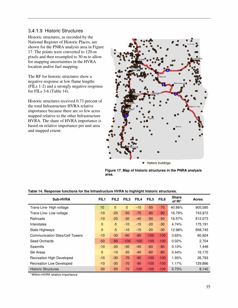
35
Historic Structures
Historic structures, as recorded by the
National Register of Historic Places, are
shown for the PNRA analysis area in Figure
17. The points were converted to 120-m
pixels and then resampled to 30 m to allow
for mapping uncertainties in the HVRA
location and/or fuel mapping.
The RF for historic structures show a
negative response at low flame lengths
(FILs 1-2) and a strongly negative response
for FILs 3-6 (Table 14).
Historic structures received 0.73 percent of
the total Infrastructure HVRA relative
importance because there are so few acres
mapped relative to the other Infrastructure
HVRA. The share of HVRA importance is
based on relative importance per unit area
and mapped extent.
Figure 17. Map of historic structures in the PNRA analysis area.
Table 14. Response functions for the Infrastructure HVRA to highlight historic structures.
Sub-HVRA FIL1 FIL2 FIL3 FIL4 FIL5 FIL6 Share of RI1
Acres
Trans-Line- High voltage 10 0 0 -10 -50 -70 40.86% 905,585
Trans-Line- Low voltage -10 -20 -50 -70 -80 -90 16.79% 743,972
Railroads -10 -20 -30 -40 -50 -50 16.57% 612,073
Interstates 0 -5 -10 -15 -20 -30 4.74% 175,191
State Highways 0 -5 -10 -15 -20 -30 12.98% 958,745
Communication Sites/Cell Towers -10 -30 -60 -80 -100 -100 3.65% 80,924
Seed Orchards -50 -90 -100 -100 -100 -100 0.02% 2,704
Sawmills -10 -20 -30 -40 -60 -80 0.10% 1,448
Ski Areas 0 -10 -20 -40 -60 -80 0.44% 16,175
Recreation High Developed -10 -30 -70 -90 -100 -100 1.93% 26,793
Recreation Low Developed -10 -30 -70 -90 -100 -100 1.17% 129,886
Historic Structures -30 -50 -70 -100 -100 -100 0.73% 8,140 1 Within-HVRA relative importance.
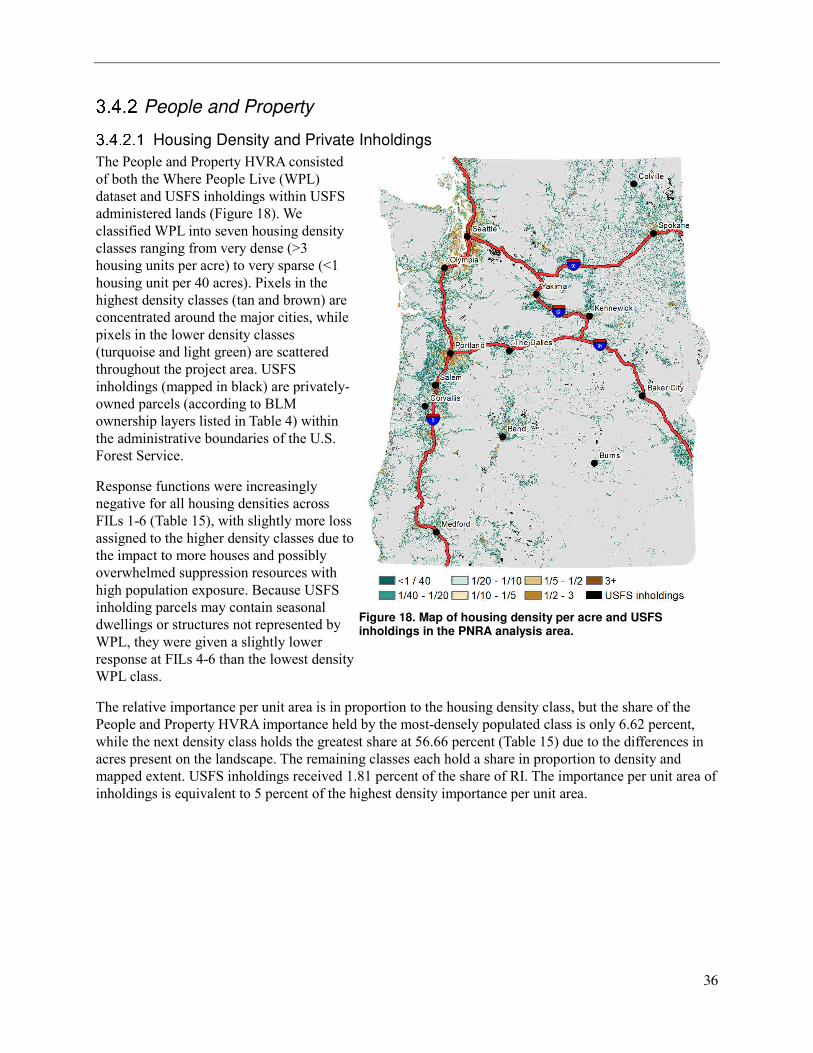
36
People and Property
Housing Density and Private Inholdings
The People and Property HVRA consisted
of both the Where People Live (WPL)
dataset and USFS inholdings within USFS
administered lands (Figure 18). We
classified WPL into seven housing density
classes ranging from very dense (>3
housing units per acre) to very sparse (<1
housing unit per 40 acres). Pixels in the
highest density classes (tan and brown) are
concentrated around the major cities, while
pixels in the lower density classes
(turquoise and light green) are scattered
throughout the project area. USFS
inholdings (mapped in black) are privately-
owned parcels (according to BLM
ownership layers listed in Table 4) within
the administrative boundaries of the U.S.
Forest Service.
Response functions were increasingly
negative for all housing densities across
FILs 1-6 (Table 15), with slightly more loss
assigned to the higher density classes due to
the impact to more houses and possibly
overwhelmed suppression resources with
high population exposure. Because USFS
inholding parcels may contain seasonal
dwellings or structures not represented by
WPL, they were given a slightly lower
response at FILs 4-6 than the lowest density
WPL class.
Figure 18. Map of housing density per acre and USFS inholdings in the PNRA analysis area.
The relative importance per unit area is in proportion to the housing density class, but the share of the
People and Property HVRA importance held by the most-densely populated class is only 6.62 percent,
while the next density class holds the greatest share at 56.66 percent (Table 15) due to the differences in
acres present on the landscape. The remaining classes each hold a share in proportion to density and
mapped extent. USFS inholdings received 1.81 percent of the share of RI. The importance per unit area of
inholdings is equivalent to 5 percent of the highest density importance per unit area.
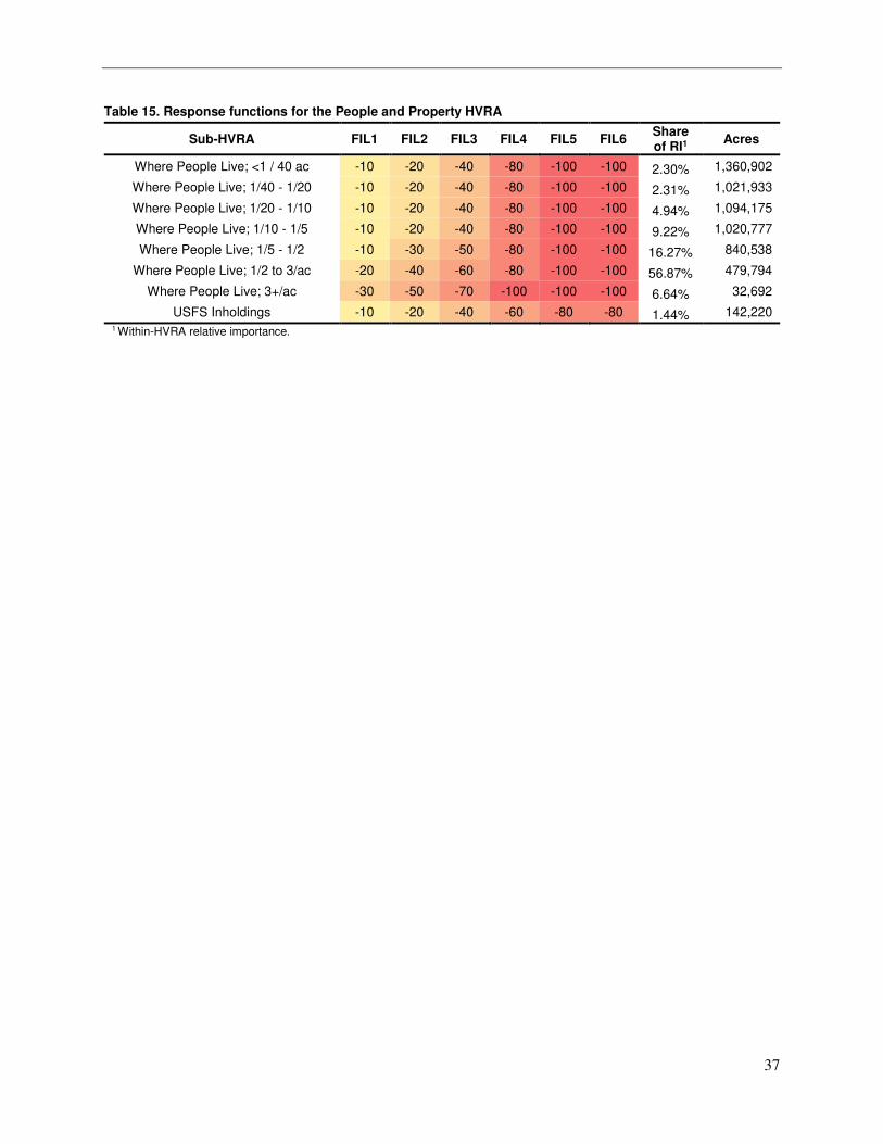
37
Table 15. Response functions for the People and Property HVRA
Sub-HVRA FIL1 FIL2 FIL3 FIL4 FIL5 FIL6 Share of RI1
Acres
Where People Live; <1 / 40 ac -10 -20 -40 -80 -100 -100 2.30% 1,360,902
Where People Live; 1/40 - 1/20 -10 -20 -40 -80 -100 -100 2.31% 1,021,933
Where People Live; 1/20 - 1/10 -10 -20 -40 -80 -100 -100 4.94% 1,094,175
Where People Live; 1/10 - 1/5 -10 -20 -40 -80 -100 -100 9.22% 1,020,777
Where People Live; 1/5 - 1/2 -10 -30 -50 -80 -100 -100 16.27% 840,538
Where People Live; 1/2 to 3/ac -20 -40 -60 -80 -100 -100 56.87% 479,794
Where People Live; 3+/ac -30 -50 -70 -100 -100 -100 6.64% 32,692
USFS Inholdings -10 -20 -40 -60 -80 -80 1.44% 142,220 1 Within-HVRA relative importance.
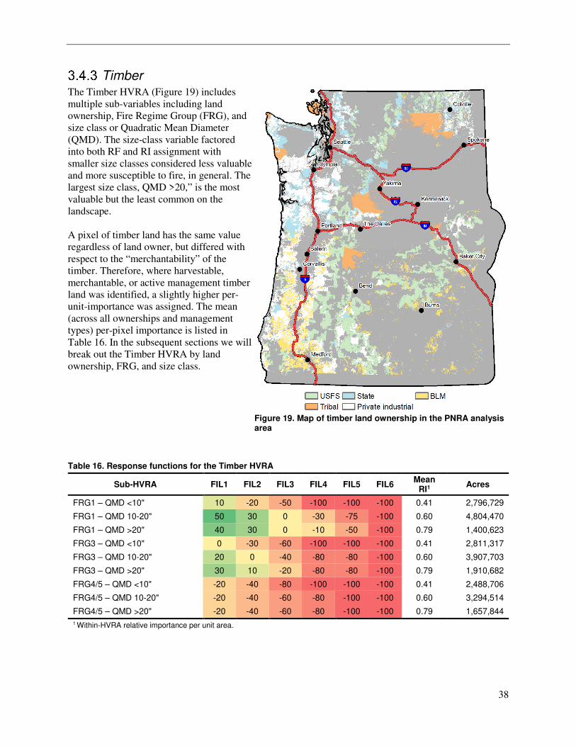
38
Timber The Timber HVRA (Figure 19) includes
multiple sub-variables including land
ownership, Fire Regime Group (FRG), and
size class or Quadratic Mean Diameter
(QMD). The size-class variable factored
into both RF and RI assignment with
smaller size classes considered less valuable
and more susceptible to fire, in general. The
largest size class, QMD >20,” is the most
valuable but the least common on the
landscape.
A pixel of timber land has the same value
regardless of land owner, but differed with
respect to the “merchantability” of the
timber. Therefore, where harvestable,
merchantable, or active management timber
land was identified, a slightly higher per-
unit-importance was assigned. The mean
(across all ownerships and management
types) per-pixel importance is listed in
Table 16. In the subsequent sections we will
break out the Timber HVRA by land
ownership, FRG, and size class.
Figure 19. Map of timber land ownership in the PNRA analysis area
Table 16. Response functions for the Timber HVRA
Sub-HVRA FIL1 FIL2 FIL3 FIL4 FIL5 FIL6 Mean
RI1 Acres
FRG1 – QMD <10" 10 -20 -50 -100 -100 -100 0.41 2,796,729
FRG1 – QMD 10-20" 50 30 0 -30 -75 -100 0.60 4,804,470
FRG1 – QMD >20" 40 30 0 -10 -50 -100 0.79 1,400,623
FRG3 – QMD <10" 0 -30 -60 -100 -100 -100 0.41 2,811,317
FRG3 – QMD 10-20" 20 0 -40 -80 -80 -100 0.60 3,907,703
FRG3 – QMD >20" 30 10 -20 -80 -80 -100 0.79 1,910,682
FRG4/5 – QMD <10" -20 -40 -80 -100 -100 -100 0.41 2,488,706
FRG4/5 – QMD 10-20" -20 -40 -60 -80 -100 -100 0.60 3,294,514
FRG4/5 – QMD >20" -20 -40 -60 -80 -100 -100 0.79 1,657,844
1 Within-HVRA relative importance per unit area.
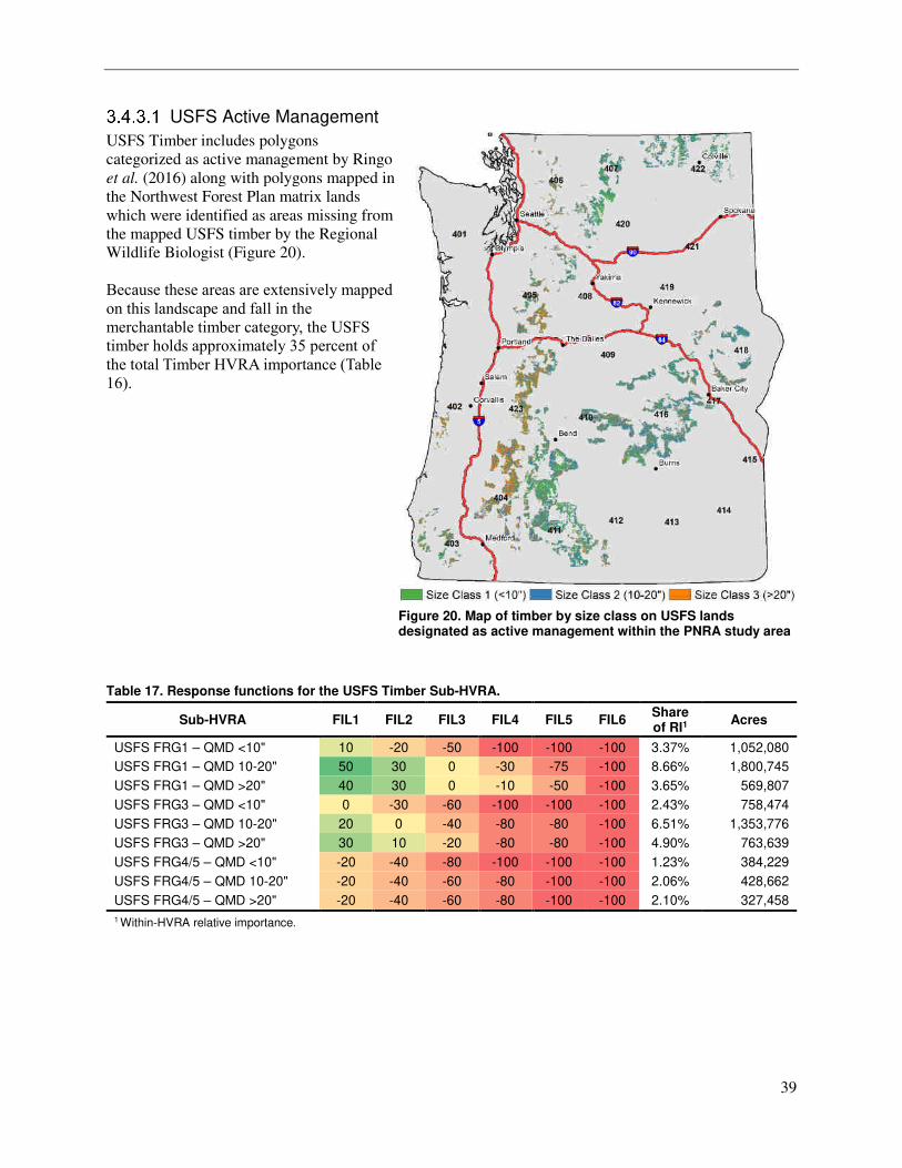
39
USFS Active Management
USFS Timber includes polygons
categorized as active management by Ringo
et al. (2016) along with polygons mapped in
the Northwest Forest Plan matrix lands
which were identified as areas missing from
the mapped USFS timber by the Regional
Wildlife Biologist (Figure 20).
Because these areas are extensively mapped
on this landscape and fall in the
merchantable timber category, the USFS
timber holds approximately 35 percent of
the total Timber HVRA importance (Table
16).
Figure 20. Map of timber by size class on USFS lands designated as active management within the PNRA study area
Table 17. Response functions for the USFS Timber Sub-HVRA.
Sub-HVRA FIL1 FIL2 FIL3 FIL4 FIL5 FIL6 Share of RI1
Acres
USFS FRG1 – QMD <10" 10 -20 -50 -100 -100 -100 3.37% 1,052,080
USFS FRG1 – QMD 10-20" 50 30 0 -30 -75 -100 8.66% 1,800,745
USFS FRG1 – QMD >20" 40 30 0 -10 -50 -100 3.65% 569,807
USFS FRG3 – QMD <10" 0 -30 -60 -100 -100 -100 2.43% 758,474
USFS FRG3 – QMD 10-20" 20 0 -40 -80 -80 -100 6.51% 1,353,776
USFS FRG3 – QMD >20" 30 10 -20 -80 -80 -100 4.90% 763,639
USFS FRG4/5 – QMD <10" -20 -40 -80 -100 -100 -100 1.23% 384,229
USFS FRG4/5 – QMD 10-20" -20 -40 -60 -80 -100 -100 2.06% 428,662
USFS FRG4/5 – QMD >20" -20 -40 -60 -80 -100 -100 2.10% 327,458
1 Within-HVRA relative importance.
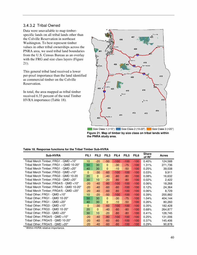
40
Tribal Owned
Data were unavailable to map timber-
specific lands on all tribal lands other than
the Colville Reservation in northeast
Washington. To best represent timber
values in other tribal ownerships across the
PNRA area, we used tribal land boundaries
from the U.S. Census Bureau as an overlay
with the FRG and size class layers (Figure
21).
This general tribal land received a lower
per-pixel importance than the land identified
as commercial timber on the Colville
Reservation.
In total, the area mapped as tribal timber
received 6.35 percent of the total Timber
HVRA importance (Table 18).
Figure 21. Map of timber by size class on tribal lands within the PNRA study area.
Table 18. Response functions for the Tribal Timber Sub-HVRA
Sub-HVRA FIL1 FIL2 FIL3 FIL4 FIL5 FIL6 Share of RI1
Acres
Tribal Merch Timber; FRG1 - QMD <10" 10 -20 -50 -100 -100 -100 0.40% 124,588
Tribal Merch Timber; FRG1 – QMD 10-20" 50 30 0 -30 -75 -100 1.31% 271,736
Tribal Merch Timber; FRG1 - QMD >20" 40 30 0 -10 -50 -100 0.25% 39,038
Tribal Merch Timber; FRG3 - QMD <10" 0 -30 -60 -100 -100 -100 0.03% 9,911
Tribal Merch Timber; FRG3 - QMD 10-20 20 0 -40 -80 -80 -100 0.08% 16,632
Tribal Merch Timber; FRG3 - QMD >20" 30 10 -20 -80 -80 -100 0.02% 2,422
Tribal Merch Timber; FRG4/5 - QMD <10" -20 -40 -80 -100 -100 -100 0.06% 18,268
Tribal Merch Timber; FRG4/5 - QMD 10-20" -20 -40 -60 -80 -100 -100 0.12% 24,364
Tribal Merch Timber; FRG4/5 - QMD >20" -20 -40 -60 -80 -100 -100 0.06% 8,729
Tribal Other; FRG1 - QMD <10" 10 -20 -50 -100 -100 -100 0.39% 200,882
Tribal Other; FRG1 - QMD 10-20" 50 30 0 -30 -75 -100 1.04% 404,144
Tribal Other; FRG1 - QMD >20" 40 30 0 -10 -50 -100 0.26% 80,260
Tribal Other; FRG3 - QMD <10" 0 -30 -60 -100 -100 -100 0.35% 182,428
Tribal Other; FRG3 - QMD 10-20" 20 0 -40 -80 -80 -100 0.68% 264,877
Tribal Other; FRG3 - QMD >20" 30 10 -20 -80 -80 -100 0.41% 128,745
Tribal Other; FRG4/5 - QMD <10" -20 -40 -80 -100 -100 -100 0.25% 131,006
Tribal Other; FRG4/5 - QMD 10-20" -20 -40 -60 -80 -100 -100 0.37% 145,406
Tribal Other; FRG4/5 - QMD >20" -20 -40 -60 -80 -100 -100 0.29% 90,878 1 Within-HVRA relative importance.
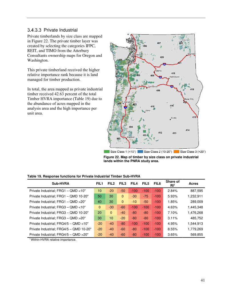
41
Private Industrial
Private timberlands by size class are mapped
in Figure 22. The private timber layer was
created by selecting the categories IFPC,
REIT, and TIMO from the Atterbury
Consultants ownership maps for Oregon and
Washington.
This private timberland received the higher
relative importance rank because it is land
managed for timber production.
In total, the area mapped as private industrial
timber received 42.63 percent of the total
Timber HVRA importance (Table 19) due to
the abundance of acres mapped in the
analysis area and the high importance per
unit area.
Figure 22. Map of timber by size class on private industrial lands within the PNRA study area.
Table 19. Response functions for Private Industrial Timber Sub-HVRA
Sub-HVRA FIL1 FIL2 FIL3 FIL4 FIL5 FIL6 Share of
RI1 Acres
Private Industrial; FRG1 – QMD <10" 10 -20 -50 -100 -100 -100 2.84% 887,595
Private Industrial; FRG1 – QMD 10-20" 50 30 0 -30 -75 -100 5.93% 1,232,911
Private Industrial; FRG1 – QMD >20" 40 30 0 -10 -50 -100 1.85% 289,009
Private Industrial; FRG3 – QMD <10" 0 -30 -60 -100 -100 -100 4.63% 1,445,348
Private Industrial; FRG3 – QMD 10-20" 20 0 -40 -80 -80 -100 7.10% 1,476,268
Private Industrial; FRG3 – QMD >20" 30 10 -20 -80 -80 -100 3.11% 485,752
Private Industrial; FRG4/5 – QMD <10" -20 -40 -80 -100 -100 -100 4.95% 1,544,913
Private Industrial; FRG4/5 – QMD 10-20" -20 -40 -60 -80 -100 -100 8.55% 1,779,269
Private Industrial; FRG4/5 – QMD >20" -20 -40 -60 -80 -100 -100 3.65% 569,855 1 Within-HVRA relative importance.
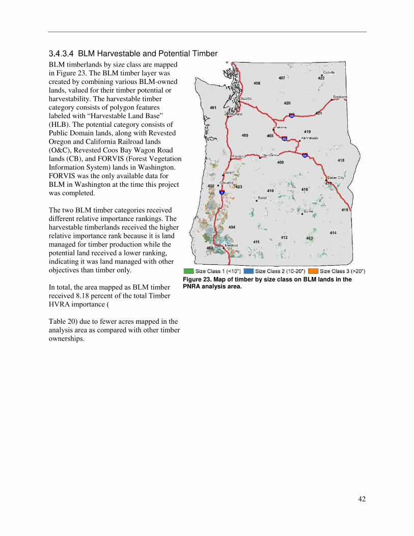
42
BLM Harvestable and Potential Timber
BLM timberlands by size class are mapped
in Figure 23. The BLM timber layer was
created by combining various BLM-owned
lands, valued for their timber potential or
harvestability. The harvestable timber
category consists of polygon features
labeled with “Harvestable Land Base”
(HLB). The potential category consists of
Public Domain lands, along with Revested
Oregon and California Railroad lands
(O&C), Revested Coos Bay Wagon Road
lands (CB), and FORVIS (Forest Vegetation
Information System) lands in Washington.
FORVIS was the only available data for
BLM in Washington at the time this project
was completed.
The two BLM timber categories received
different relative importance rankings. The
harvestable timberlands received the higher
relative importance rank because it is land
managed for timber production while the
potential land received a lower ranking,
indicating it was land managed with other
objectives than timber only.
In total, the area mapped as BLM timber
received 8.18 percent of the total Timber
HVRA importance (
Table 20) due to fewer acres mapped in the
analysis area as compared with other timber
ownerships.
Figure 23. Map of timber by size class on BLM lands in the PNRA analysis area.
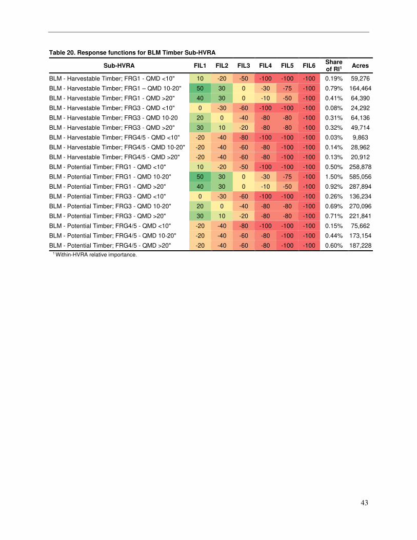
43
Table 20. Response functions for BLM Timber Sub-HVRA
Sub-HVRA FIL1 FIL2 FIL3 FIL4 FIL5 FIL6 Share of RI1
Acres
BLM - Harvestable Timber; FRG1 - QMD <10" 10 -20 -50 -100 -100 -100 0.19% 59,276
BLM - Harvestable Timber; FRG1 – QMD 10-20" 50 30 0 -30 -75 -100 0.79% 164,464
BLM - Harvestable Timber; FRG1 - QMD >20" 40 30 0 -10 -50 -100 0.41% 64,390
BLM - Harvestable Timber; FRG3 - QMD <10" 0 -30 -60 -100 -100 -100 0.08% 24,292
BLM - Harvestable Timber; FRG3 - QMD 10-20 20 0 -40 -80 -80 -100 0.31% 64,136
BLM - Harvestable Timber; FRG3 - QMD >20" 30 10 -20 -80 -80 -100 0.32% 49,714
BLM - Harvestable Timber; FRG4/5 - QMD <10" -20 -40 -80 -100 -100 -100 0.03% 9,863
BLM - Harvestable Timber; FRG4/5 - QMD 10-20" -20 -40 -60 -80 -100 -100 0.14% 28,962
BLM - Harvestable Timber; FRG4/5 - QMD >20" -20 -40 -60 -80 -100 -100 0.13% 20,912
BLM - Potential Timber; FRG1 - QMD <10" 10 -20 -50 -100 -100 -100 0.50% 258,878
BLM - Potential Timber; FRG1 - QMD 10-20" 50 30 0 -30 -75 -100 1.50% 585,056
BLM - Potential Timber; FRG1 - QMD >20" 40 30 0 -10 -50 -100 0.92% 287,894
BLM - Potential Timber; FRG3 - QMD <10" 0 -30 -60 -100 -100 -100 0.26% 136,234
BLM - Potential Timber; FRG3 - QMD 10-20" 20 0 -40 -80 -80 -100 0.69% 270,096
BLM - Potential Timber; FRG3 - QMD >20" 30 10 -20 -80 -80 -100 0.71% 221,841
BLM - Potential Timber; FRG4/5 - QMD <10" -20 -40 -80 -100 -100 -100 0.15% 75,662
BLM - Potential Timber; FRG4/5 - QMD 10-20" -20 -40 -60 -80 -100 -100 0.44% 173,154
BLM - Potential Timber; FRG4/5 - QMD >20" -20 -40 -60 -80 -100 -100 0.60% 187,228 1 Within-HVRA relative importance.
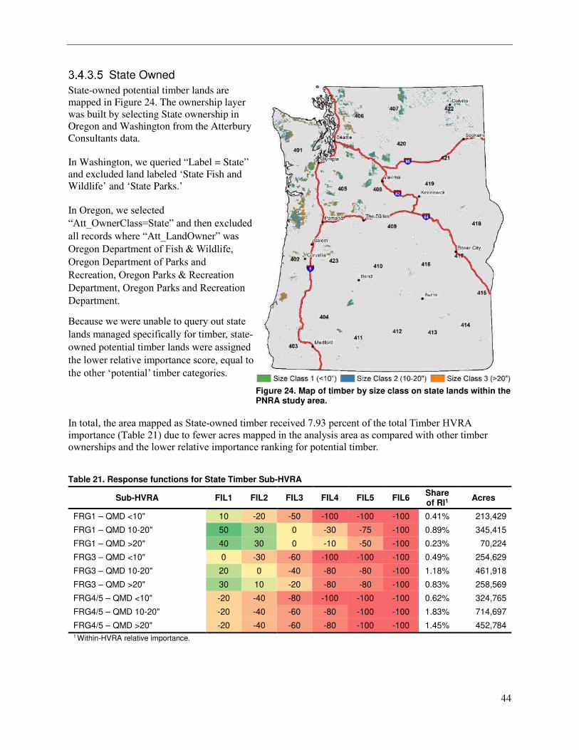
44
State Owned
State-owned potential timber lands are
mapped in Figure 24. The ownership layer
was built by selecting State ownership in
Oregon and Washington from the Atterbury
Consultants data.
In Washington, we queried “Label = State”
and excluded land labeled ‘State Fish and
Wildlife’ and ‘State Parks.’
In Oregon, we selected
“Att_OwnerClass=State” and then excluded
all records where “Att_LandOwner” was
Oregon Department of Fish & Wildlife,
Oregon Department of Parks and
Recreation, Oregon Parks & Recreation
Department, Oregon Parks and Recreation
Department.
Because we were unable to query out state
lands managed specifically for timber, state-
owned potential timber lands were assigned
the lower relative importance score, equal to
the other ‘potential’ timber categories.
Figure 24. Map of timber by size class on state lands within the PNRA study area.
In total, the area mapped as State-owned timber received 7.93 percent of the total Timber HVRA
importance (Table 21) due to fewer acres mapped in the analysis area as compared with other timber
ownerships and the lower relative importance ranking for potential timber.
Table 21. Response functions for State Timber Sub-HVRA
Sub-HVRA FIL1 FIL2 FIL3 FIL4 FIL5 FIL6 Share of RI1
Acres
FRG1 – QMD <10" 10 -20 -50 -100 -100 -100 0.41% 213,429
FRG1 – QMD 10-20" 50 30 0 -30 -75 -100 0.89% 345,415
FRG1 – QMD >20" 40 30 0 -10 -50 -100 0.23% 70,224
FRG3 – QMD <10" 0 -30 -60 -100 -100 -100 0.49% 254,629
FRG3 – QMD 10-20" 20 0 -40 -80 -80 -100 1.18% 461,918
FRG3 – QMD >20" 30 10 -20 -80 -80 -100 0.83% 258,569
FRG4/5 – QMD <10" -20 -40 -80 -100 -100 -100 0.62% 324,765
FRG4/5 – QMD 10-20" -20 -40 -60 -80 -100 -100 1.83% 714,697
FRG4/5 – QMD >20" -20 -40 -60 -80 -100 -100 1.45% 452,784 1 Within-HVRA relative importance.
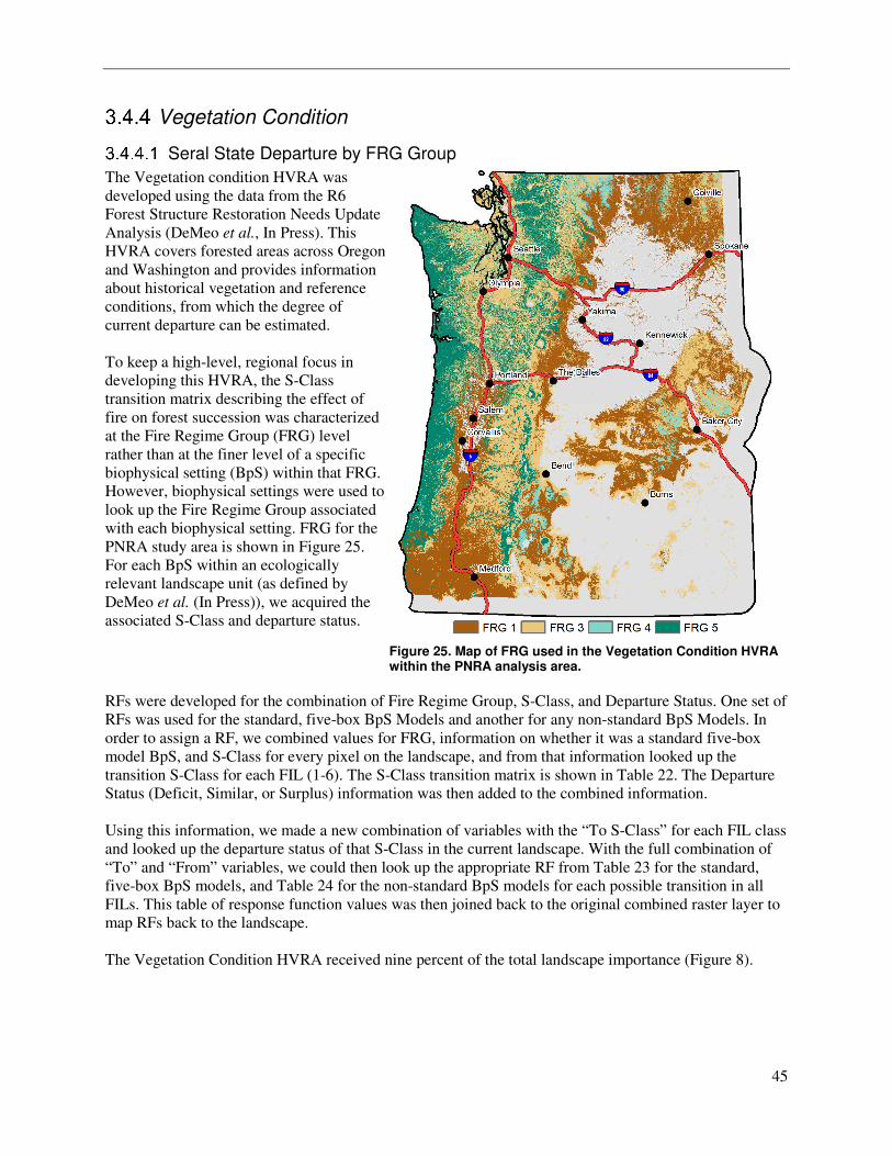
45
Vegetation Condition
Seral State Departure by FRG Group
The Vegetation condition HVRA was
developed using the data from the R6
Forest Structure Restoration Needs Update
Analysis (DeMeo et al., In Press). This
HVRA covers forested areas across Oregon
and Washington and provides information
about historical vegetation and reference
conditions, from which the degree of
current departure can be estimated.
To keep a high-level, regional focus in
developing this HVRA, the S-Class
transition matrix describing the effect of
fire on forest succession was characterized
at the Fire Regime Group (FRG) level
rather than at the finer level of a specific
biophysical setting (BpS) within that FRG.
However, biophysical settings were used to
look up the Fire Regime Group associated
with each biophysical setting. FRG for the
PNRA study area is shown in Figure 25.
For each BpS within an ecologically
relevant landscape unit (as defined by
DeMeo et al. (In Press)), we acquired the
associated S-Class and departure status.
Figure 25. Map of FRG used in the Vegetation Condition HVRA within the PNRA analysis area.
RFs were developed for the combination of Fire Regime Group, S-Class, and Departure Status. One set of
RFs was used for the standard, five-box BpS Models and another for any non-standard BpS Models. In
order to assign a RF, we combined values for FRG, information on whether it was a standard five-box
model BpS, and S-Class for every pixel on the landscape, and from that information looked up the
transition S-Class for each FIL (1-6). The S-Class transition matrix is shown in Table 22. The Departure
Status (Deficit, Similar, or Surplus) information was then added to the combined information.
Using this information, we made a new combination of variables with the “To S-Class” for each FIL class
and looked up the departure status of that S-Class in the current landscape. With the full combination of
“To” and “From” variables, we could then look up the appropriate RF from Table 23 for the standard,
five-box BpS models, and Table 24 for the non-standard BpS models for each possible transition in all
FILs. This table of response function values was then joined back to the original combined raster layer to
map RFs back to the landscape.
The Vegetation Condition HVRA received nine percent of the total landscape importance (Figure 8).
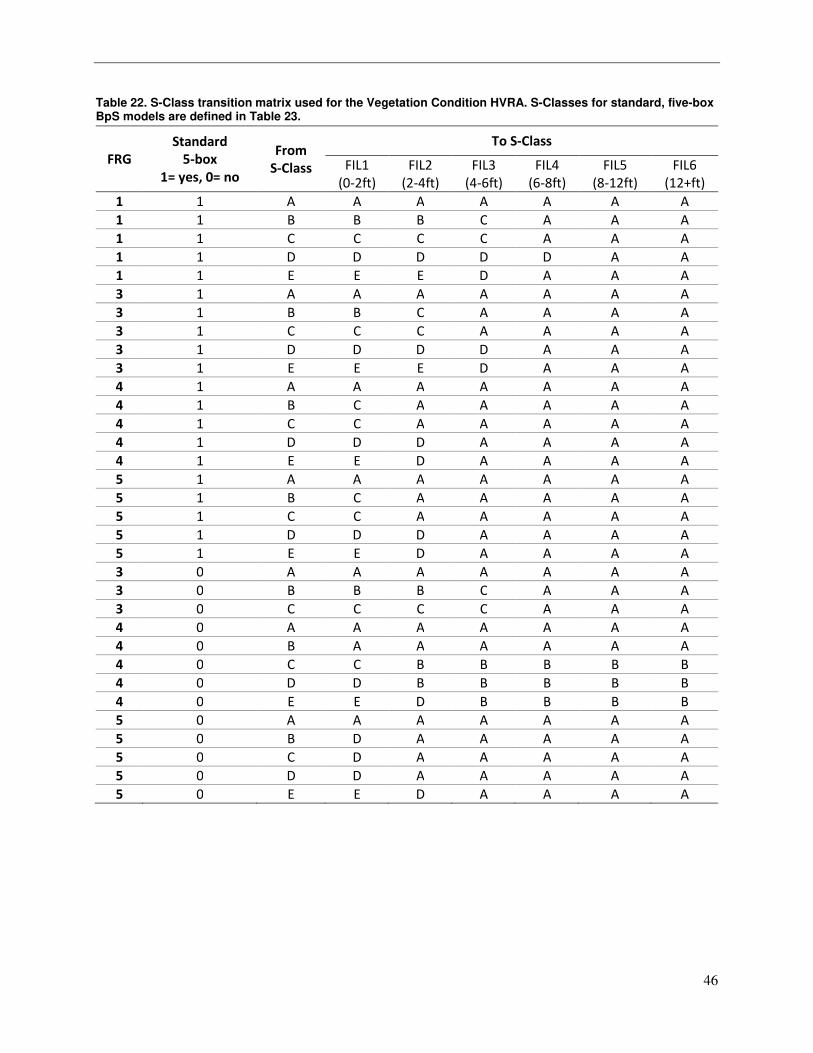
46
Table 22. S-Class transition matrix used for the Vegetation Condition HVRA. S-Classes for standard, five-box BpS models are defined in Table 23.
FRG
Standard
5-box
1= yes, 0= no
From
S-Class
To S-Class
FIL1
(0-2ft)
FIL2
(2-4ft)
FIL3
(4-6ft)
FIL4
(6-8ft)
FIL5
(8-12ft)
FIL6
(12+ft)
1 1 A A A A A A A
1 1 B B B C A A A
1 1 C C C C A A A
1 1 D D D D D A A
1 1 E E E D A A A
3 1 A A A A A A A
3 1 B B C A A A A
3 1 C C C A A A A
3 1 D D D D A A A
3 1 E E E D A A A
4 1 A A A A A A A
4 1 B C A A A A A
4 1 C C A A A A A
4 1 D D D A A A A
4 1 E E D A A A A
5 1 A A A A A A A
5 1 B C A A A A A
5 1 C C A A A A A
5 1 D D D A A A A
5 1 E E D A A A A
3 0 A A A A A A A
3 0 B B B C A A A
3 0 C C C C A A A
4 0 A A A A A A A
4 0 B A A A A A A
4 0 C C B B B B B
4 0 D D B B B B B
4 0 E E D B B B B
5 0 A A A A A A A
5 0 B D A A A A A
5 0 C D A A A A A
5 0 D D A A A A A
5 0 E E D A A A A
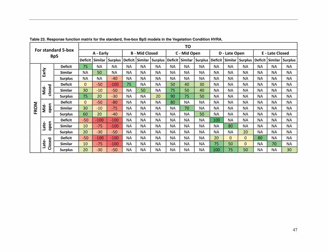
47
Table 23. Response function matrix for the standard, five-box BpS models in the Vegetation Condition HVRA.
For standard 5-box
BpS
TO
A - Early B - Mid Closed C - Mid Open D - Late Open E - Late Closed
Deficit Similar Surplus Deficit Similar Surplus Deficit Similar Surplus Deficit Similar Surplus Deficit Similar Surplus
FR
OM
Ea
rly
Deficit 75 NA NA NA NA NA NA NA NA NA NA NA NA NA NA
Similar NA 50 NA NA NA NA NA NA NA NA NA NA NA NA NA
Surplus NA NA -40 NA NA NA NA NA NA NA NA NA NA NA NA
Mid
-
clo
sed
Deficit 0 -50 -100 75 NA NA 50 40 30 NA NA NA NA NA NA
Similar 30 -10 -50 NA 50 NA 75 50 40 NA NA NA NA NA NA
Surplus 75 20 -30 NA NA 20 90 75 50 NA NA NA NA NA NA
Mid
-
op
en
Deficit 0 -50 -80 NA NA NA 80 NA NA NA NA NA NA NA NA
Similar 30 -10 -75 NA NA NA NA 70 NA NA NA NA NA NA NA
Surplus 60 20 -40 NA NA NA NA NA 50 NA NA NA NA NA NA
Late
-
op
en
Deficit -50 -100 -100 NA NA NA NA NA NA 100 NA NA NA NA NA
Similar 10 -75 -100 NA NA NA NA NA NA NA 80 NA NA NA NA
Surplus 20 -30 -50 NA NA NA NA NA NA NA NA 20 NA NA NA
Late
-
Clo
sed
Deficit -50 -100 -100 NA NA NA NA NA NA 20 0 0 80 NA NA
Similar 10 -75 -100 NA NA NA NA NA NA 75 50 0 NA 70 NA
Surplus 20 -30 -50 NA NA NA NA NA NA 100 75 50 NA NA 30
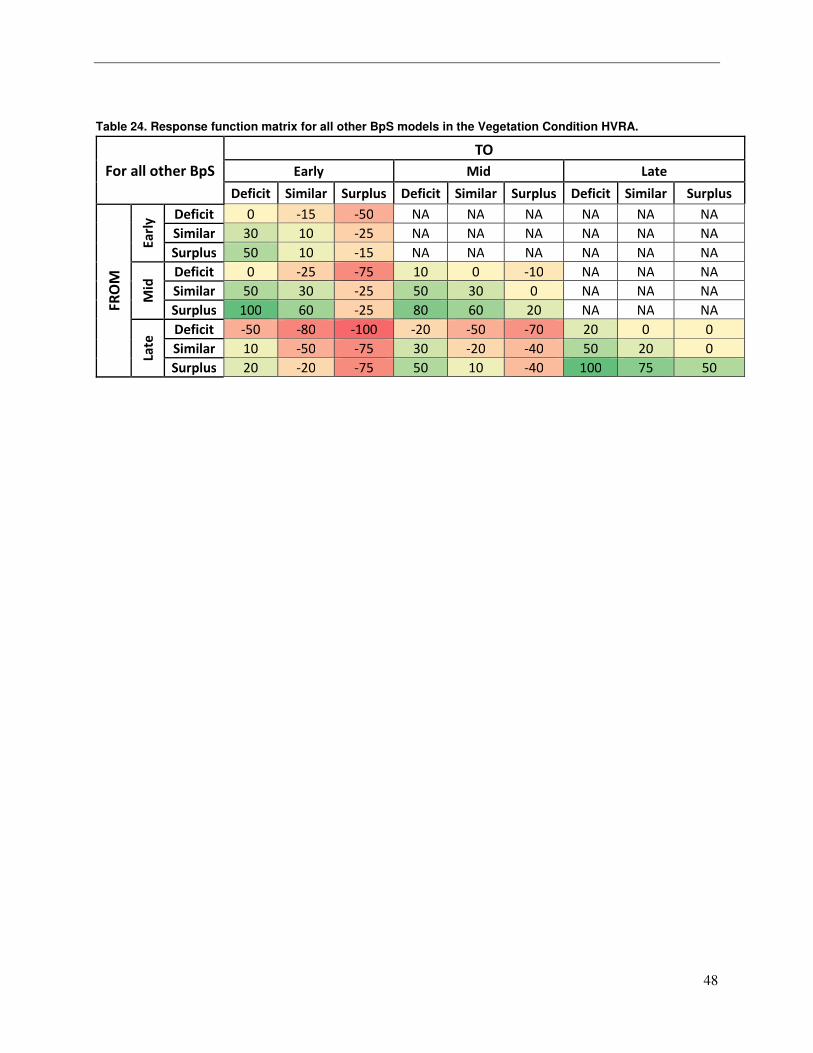
48
Table 24. Response function matrix for all other BpS models in the Vegetation Condition HVRA.
For all other BpS
TO
Early Mid Late
Deficit Similar Surplus Deficit Similar Surplus Deficit Similar Surplus
FR
OM
Ea
rly
Deficit 0 -15 -50 NA NA NA NA NA NA
Similar 30 10 -25 NA NA NA NA NA NA
Surplus 50 10 -15 NA NA NA NA NA NA
Mid
Deficit 0 -25 -75 10 0 -10 NA NA NA
Similar 50 30 -25 50 30 0 NA NA NA
Surplus 100 60 -25 80 60 20 NA NA NA
Late
Deficit -50 -80 -100 -20 -50 -70 20 0 0
Similar 10 -50 -75 30 -20 -40 50 20 0
Surplus 20 -20 -75 50 10 -40 100 75 50
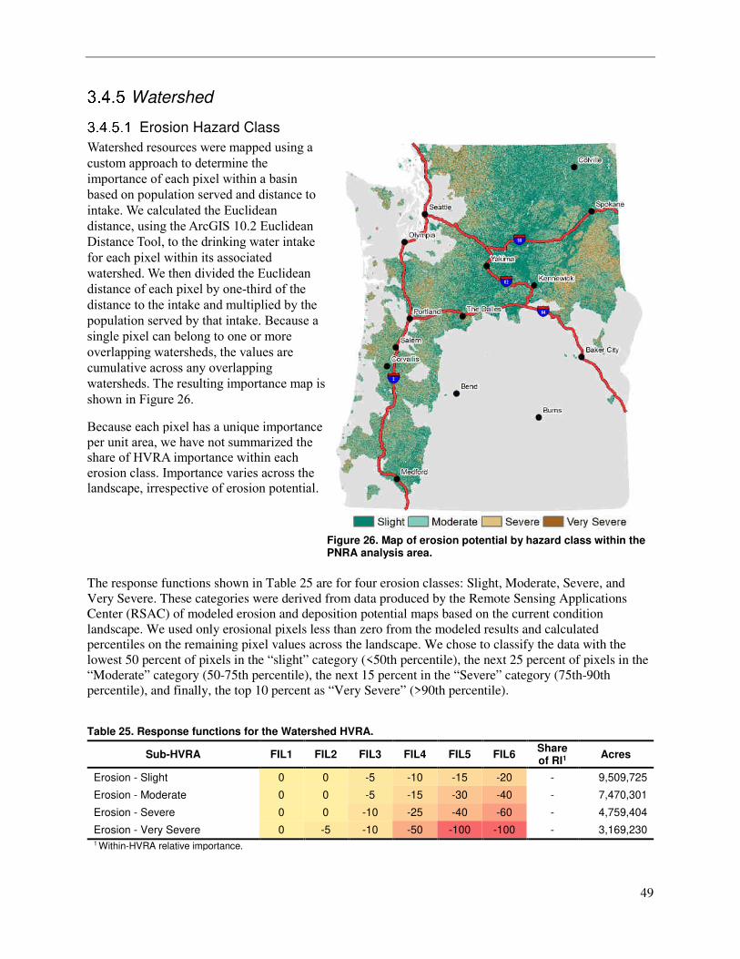
49
Watershed
Erosion Hazard Class
Watershed resources were mapped using a
custom approach to determine the
importance of each pixel within a basin
based on population served and distance to
intake. We calculated the Euclidean
distance, using the ArcGIS 10.2 Euclidean
Distance Tool, to the drinking water intake
for each pixel within its associated
watershed. We then divided the Euclidean
distance of each pixel by one-third of the
distance to the intake and multiplied by the
population served by that intake. Because a
single pixel can belong to one or more
overlapping watersheds, the values are
cumulative across any overlapping
watersheds. The resulting importance map is
shown in Figure 26.
Because each pixel has a unique importance
per unit area, we have not summarized the
share of HVRA importance within each
erosion class. Importance varies across the
landscape, irrespective of erosion potential.
Figure 26. Map of erosion potential by hazard class within the PNRA analysis area.
The response functions shown in Table 25 are for four erosion classes: Slight, Moderate, Severe, and
Very Severe. These categories were derived from data produced by the Remote Sensing Applications
Center (RSAC) of modeled erosion and deposition potential maps based on the current condition
landscape. We used only erosional pixels less than zero from the modeled results and calculated
percentiles on the remaining pixel values across the landscape. We chose to classify the data with the
lowest 50 percent of pixels in the “slight” category (<50th percentile), the next 25 percent of pixels in the
“Moderate” category (50-75th percentile), the next 15 percent in the “Severe” category (75th-90th
percentile), and finally, the top 10 percent as “Very Severe” (>90th percentile).
Table 25. Response functions for the Watershed HVRA.
Sub-HVRA FIL1 FIL2 FIL3 FIL4 FIL5 FIL6 Share of RI1
Acres
Erosion - Slight 0 0 -5 -10 -15 -20 - 9,509,725
Erosion - Moderate 0 0 -5 -15 -30 -40 - 7,470,301
Erosion - Severe 0 0 -10 -25 -40 -60 - 4,759,404
Erosion - Very Severe 0 -5 -10 -50 -100 -100 - 3,169,230 1 Within-HVRA relative importance.
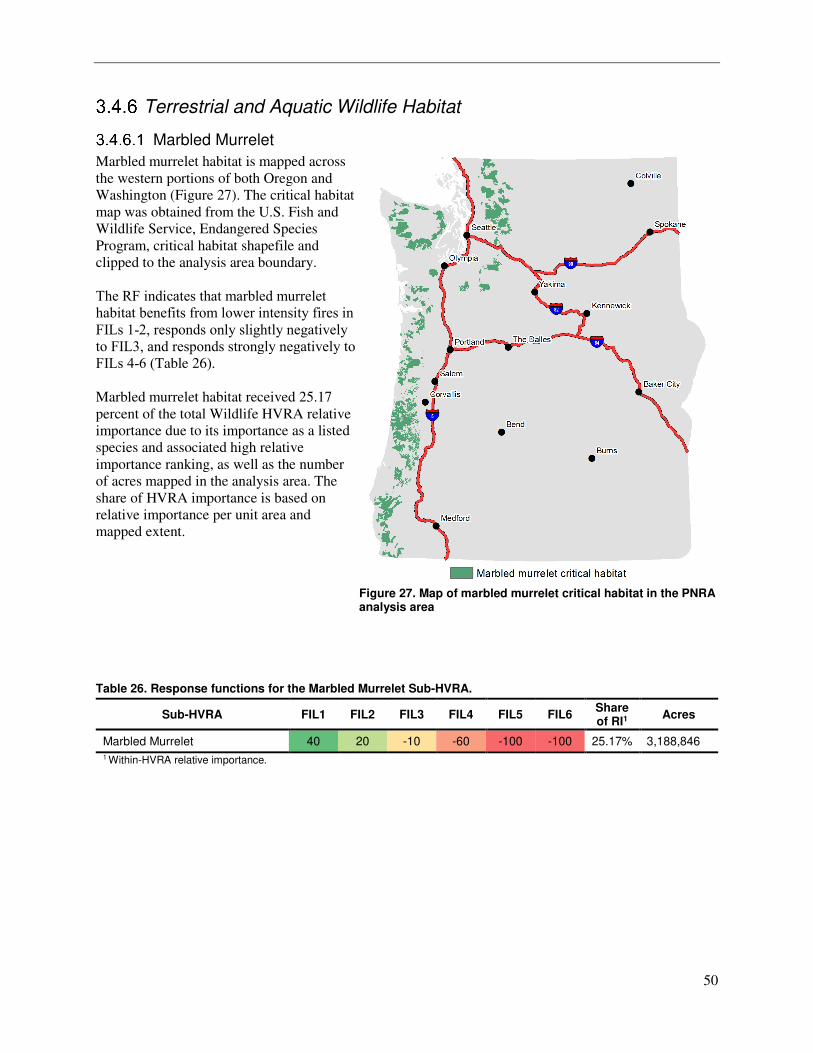
50
Terrestrial and Aquatic Wildlife Habitat
Marbled Murrelet
Marbled murrelet habitat is mapped across
the western portions of both Oregon and
Washington (Figure 27). The critical habitat
map was obtained from the U.S. Fish and
Wildlife Service, Endangered Species
Program, critical habitat shapefile and
clipped to the analysis area boundary.
The RF indicates that marbled murrelet
habitat benefits from lower intensity fires in
FILs 1-2, responds only slightly negatively
to FIL3, and responds strongly negatively to
FILs 4-6 (Table 26).
Marbled murrelet habitat received 25.17
percent of the total Wildlife HVRA relative
importance due to its importance as a listed
species and associated high relative
importance ranking, as well as the number
of acres mapped in the analysis area. The
share of HVRA importance is based on
relative importance per unit area and
mapped extent.
Figure 27. Map of marbled murrelet critical habitat in the PNRA analysis area
Table 26. Response functions for the Marbled Murrelet Sub-HVRA.
Sub-HVRA FIL1 FIL2 FIL3 FIL4 FIL5 FIL6 Share of RI1
Acres
Marbled Murrelet 40 20 -10 -60 -100 -100 25.17% 3,188,846 1 Within-HVRA relative importance.
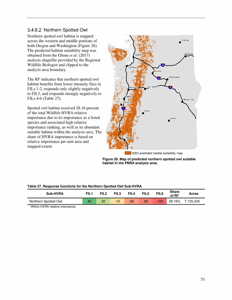
51
Northern Spotted Owl
Northern spotted owl habitat is mapped
across the western and middle portions of
both Oregon and Washington (Figure 28).
The predicted habitat suitability map was
obtained from the Glenn et al. (2017)
analysis shapefile provided by the Regional
Wildlife Biologist and clipped to the
analysis area boundary.
The RF indicates that northern spotted owl
habitat benefits from lower intensity fires in
FILs 1-2, responds only slightly negatively
to FIL3, and responds strongly negatively to
FILs 4-6 (Table 27).
Spotted owl habitat received 28.16 percent
of the total Wildlife HVRA relative
importance due to its importance as a listed
species and associated high relative
importance ranking, as well as its abundant
suitable habitat within the analysis area. The
share of HVRA importance is based on
relative importance per unit area and
mapped extent.
Figure 28. Map of predicted northern spotted owl suitable habitat in the PNRA analysis area.
Table 27. Response functions for the Northern Spotted Owl Sub-HVRA.
Sub-HVRA FIL1 FIL2 FIL3 FIL4 FIL5 FIL6 Share of RI1
Acres
Northern Spotted Owl 40 20 -10 -60 -80 -100 28.16% 7,135,435 1 Within-HVRA relative importance.
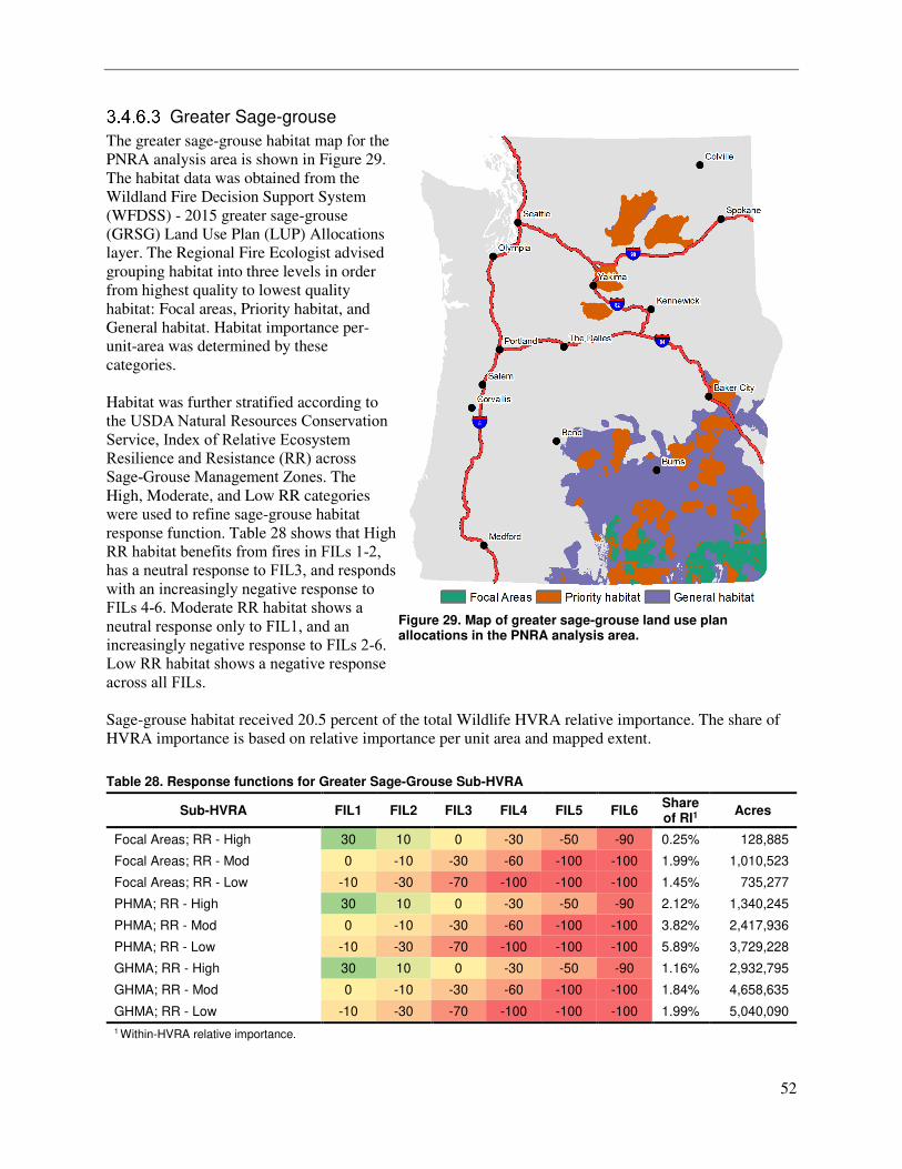
52
Greater Sage-grouse
The greater sage-grouse habitat map for the
PNRA analysis area is shown in Figure 29.
The habitat data was obtained from the
Wildland Fire Decision Support System
(WFDSS) - 2015 greater sage-grouse
(GRSG) Land Use Plan (LUP) Allocations
layer. The Regional Fire Ecologist advised
grouping habitat into three levels in order
from highest quality to lowest quality
habitat: Focal areas, Priority habitat, and
General habitat. Habitat importance per-
unit-area was determined by these
categories.
Habitat was further stratified according to
the USDA Natural Resources Conservation
Service, Index of Relative Ecosystem
Resilience and Resistance (RR) across
Sage-Grouse Management Zones. The
High, Moderate, and Low RR categories
were used to refine sage-grouse habitat
response function. Table 28 shows that High
RR habitat benefits from fires in FILs 1-2,
has a neutral response to FIL3, and responds
with an increasingly negative response to
FILs 4-6. Moderate RR habitat shows a
neutral response only to FIL1, and an
increasingly negative response to FILs 2-6.
Low RR habitat shows a negative response
across all FILs.
Figure 29. Map of greater sage-grouse land use plan allocations in the PNRA analysis area.
Sage-grouse habitat received 20.5 percent of the total Wildlife HVRA relative importance. The share of
HVRA importance is based on relative importance per unit area and mapped extent.
Table 28. Response functions for Greater Sage-Grouse Sub-HVRA
Sub-HVRA FIL1 FIL2 FIL3 FIL4 FIL5 FIL6 Share of RI1
Acres
Focal Areas; RR - High 30 10 0 -30 -50 -90 0.25% 128,885
Focal Areas; RR - Mod 0 -10 -30 -60 -100 -100 1.99% 1,010,523
Focal Areas; RR - Low -10 -30 -70 -100 -100 -100 1.45% 735,277
PHMA; RR - High 30 10 0 -30 -50 -90 2.12% 1,340,245
PHMA; RR - Mod 0 -10 -30 -60 -100 -100 3.82% 2,417,936
PHMA; RR - Low -10 -30 -70 -100 -100 -100 5.89% 3,729,228
GHMA; RR - High 30 10 0 -30 -50 -90 1.16% 2,932,795
GHMA; RR - Mod 0 -10 -30 -60 -100 -100 1.84% 4,658,635
GHMA; RR - Low -10 -30 -70 -100 -100 -100 1.99% 5,040,090
1 Within-HVRA relative importance.
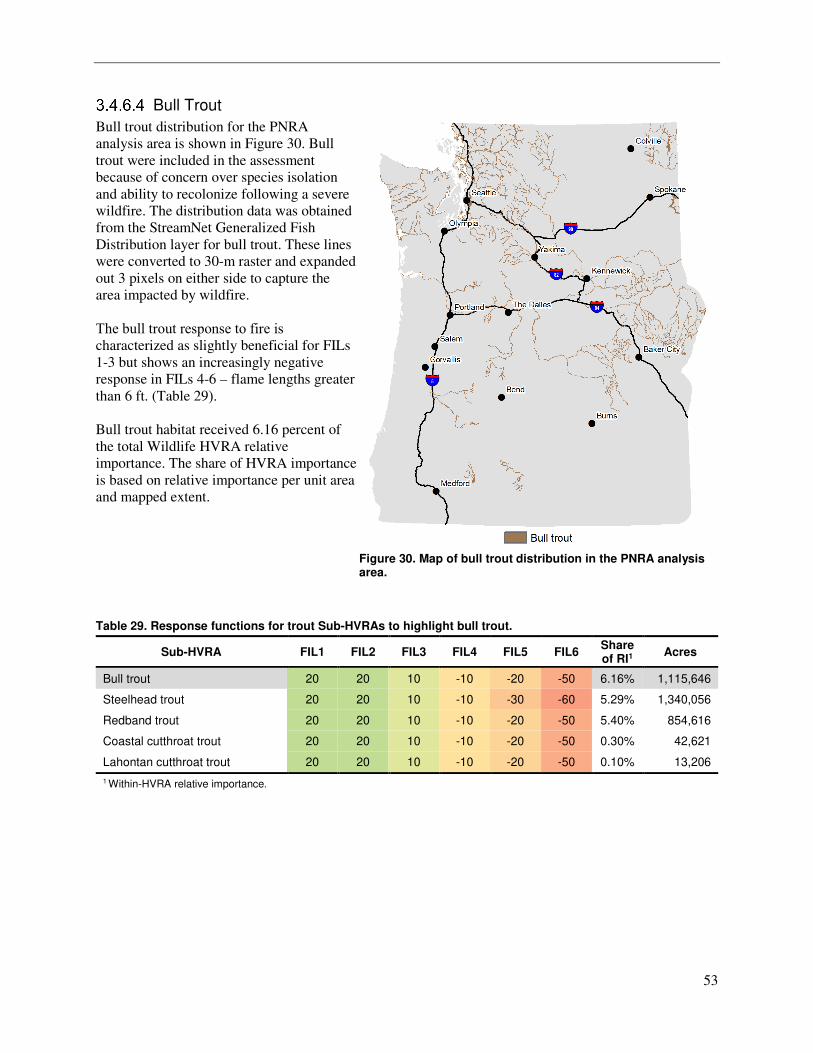
53
Bull Trout
Bull trout distribution for the PNRA
analysis area is shown in Figure 30. Bull
trout were included in the assessment
because of concern over species isolation
and ability to recolonize following a severe
wildfire. The distribution data was obtained
from the StreamNet Generalized Fish
Distribution layer for bull trout. These lines
were converted to 30-m raster and expanded
out 3 pixels on either side to capture the
area impacted by wildfire.
The bull trout response to fire is
characterized as slightly beneficial for FILs
1-3 but shows an increasingly negative
response in FILs 4-6 – flame lengths greater
than 6 ft. (Table 29).
Bull trout habitat received 6.16 percent of
the total Wildlife HVRA relative
importance. The share of HVRA importance
is based on relative importance per unit area
and mapped extent.
Figure 30. Map of bull trout distribution in the PNRA analysis area.
Table 29. Response functions for trout Sub-HVRAs to highlight bull trout.
Sub-HVRA FIL1 FIL2 FIL3 FIL4 FIL5 FIL6 Share of RI1
Acres
Bull trout 20 20 10 -10 -20 -50 6.16% 1,115,646
Steelhead trout 20 20 10 -10 -30 -60 5.29% 1,340,056
Redband trout 20 20 10 -10 -20 -50 5.40% 854,616
Coastal cutthroat trout 20 20 10 -10 -20 -50 0.30% 42,621
Lahontan cutthroat trout 20 20 10 -10 -20 -50 0.10% 13,206
1 Within-HVRA relative importance.
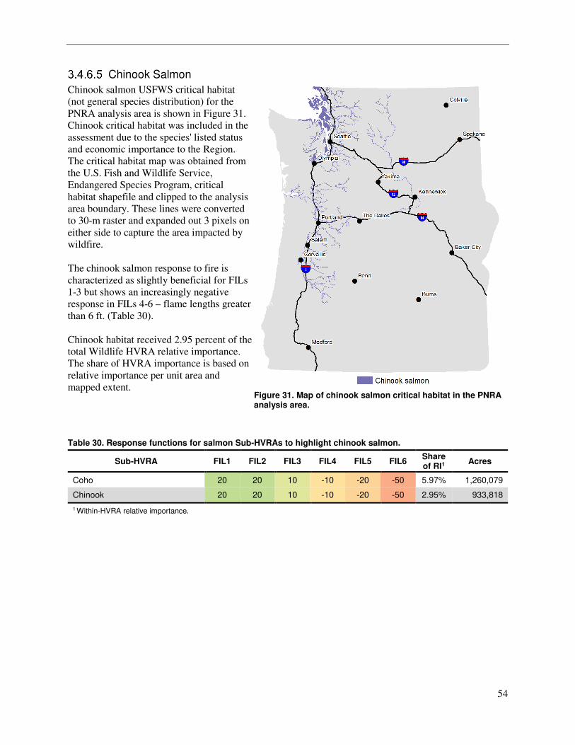
54
Chinook Salmon
Chinook salmon USFWS critical habitat
(not general species distribution) for the
PNRA analysis area is shown in Figure 31.
Chinook critical habitat was included in the
assessment due to the species' listed status
and economic importance to the Region.
The critical habitat map was obtained from
the U.S. Fish and Wildlife Service,
Endangered Species Program, critical
habitat shapefile and clipped to the analysis
area boundary. These lines were converted
to 30-m raster and expanded out 3 pixels on
either side to capture the area impacted by
wildfire.
The chinook salmon response to fire is
characterized as slightly beneficial for FILs
1-3 but shows an increasingly negative
response in FILs 4-6 – flame lengths greater
than 6 ft. (Table 30).
Chinook habitat received 2.95 percent of the
total Wildlife HVRA relative importance.
The share of HVRA importance is based on
relative importance per unit area and
mapped extent.
Figure 31. Map of chinook salmon critical habitat in the PNRA analysis area.
Table 30. Response functions for salmon Sub-HVRAs to highlight chinook salmon.
Sub-HVRA FIL1 FIL2 FIL3 FIL4 FIL5 FIL6 Share of RI1
Acres
Coho 20 20 10 -10 -20 -50 5.97% 1,260,079
Chinook 20 20 10 -10 -20 -50 2.95% 933,818
1 Within-HVRA relative importance.
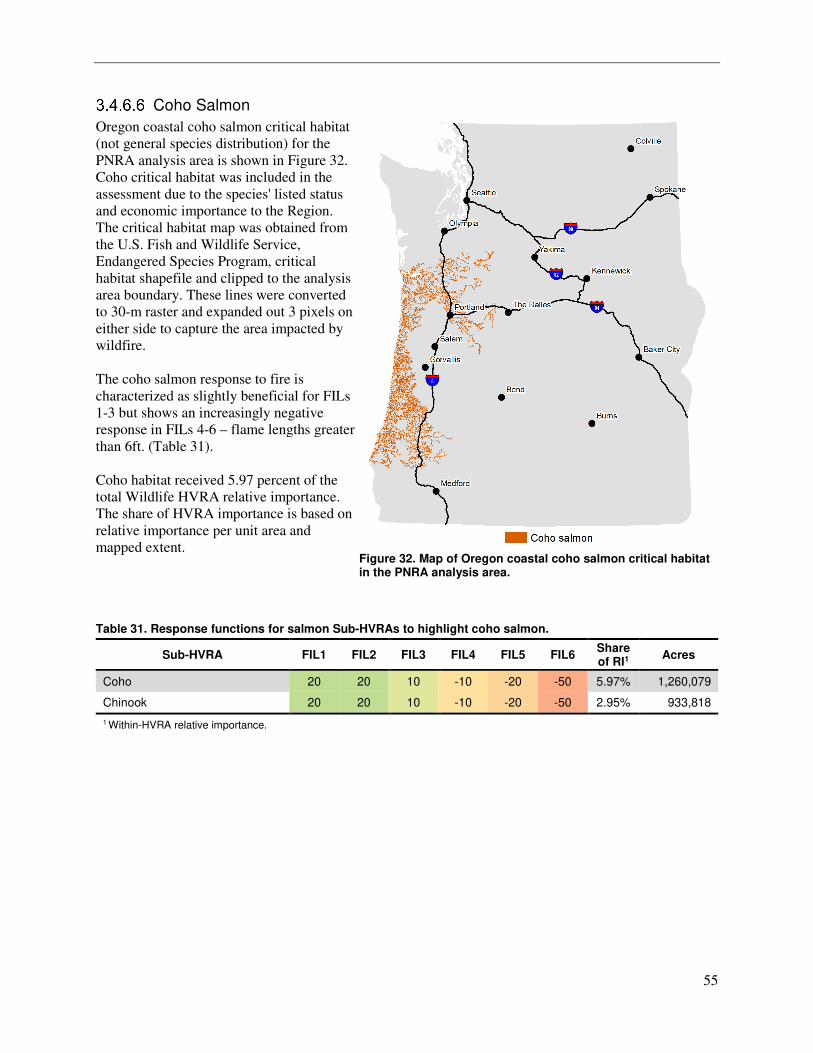
55
Coho Salmon
Oregon coastal coho salmon critical habitat
(not general species distribution) for the
PNRA analysis area is shown in Figure 32.
Coho critical habitat was included in the
assessment due to the species' listed status
and economic importance to the Region.
The critical habitat map was obtained from
the U.S. Fish and Wildlife Service,
Endangered Species Program, critical
habitat shapefile and clipped to the analysis
area boundary. These lines were converted
to 30-m raster and expanded out 3 pixels on
either side to capture the area impacted by
wildfire.
The coho salmon response to fire is
characterized as slightly beneficial for FILs
1-3 but shows an increasingly negative
response in FILs 4-6 – flame lengths greater
than 6ft. (Table 31).
Coho habitat received 5.97 percent of the
total Wildlife HVRA relative importance.
The share of HVRA importance is based on
relative importance per unit area and
mapped extent.
Figure 32. Map of Oregon coastal coho salmon critical habitat in the PNRA analysis area.
Table 31. Response functions for salmon Sub-HVRAs to highlight coho salmon.
Sub-HVRA FIL1 FIL2 FIL3 FIL4 FIL5 FIL6 Share of RI1
Acres
Coho 20 20 10 -10 -20 -50 5.97% 1,260,079
Chinook 20 20 10 -10 -20 -50 2.95% 933,818
1 Within-HVRA relative importance.
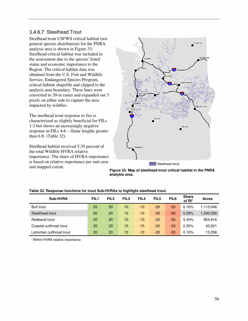
56
Steelhead Trout
Steelhead trout USFWS critical habitat (not
general species distribution) for the PNRA
analysis area is shown in Figure 33.
Steelhead critical habitat was included in
the assessment due to the species' listed
status and economic importance to the
Region. The critical habitat data was
obtained from the U.S. Fish and Wildlife
Service, Endangered Species Program,
critical habitat shapefile and clipped to the
analysis area boundary. These lines were
converted to 30-m raster and expanded out 3
pixels on either side to capture the area
impacted by wildfire.
The steelhead trout response to fire is
characterized as slightly beneficial for FILs
1-3 but shows an increasingly negative
response in FILs 4-6 – flame lengths greater
than 6 ft. (Table 32).
Steelhead habitat received 5.29 percent of
the total Wildlife HVRA relative
importance. The share of HVRA importance
is based on relative importance per unit area
and mapped extent.
Figure 33. Map of steelhead trout critical habitat in the PNRA analysis area.
Table 32. Response functions for trout Sub-HVRAs to highlight steelhead trout.
Sub-HVRA FIL1 FIL2 FIL3 FIL4 FIL5 FIL6 Share of RI1
Acres
Bull trout 20 20 10 -10 -20 -50 6.16% 1,115,646
Steelhead trout 20 20 10 -10 -30 -60 5.29% 1,340,056
Redband trout 20 20 10 -10 -20 -50 5.40% 854,616
Coastal cutthroat trout 20 20 10 -10 -20 -50 0.30% 42,621
Lahontan cutthroat trout 20 20 10 -10 -20 -50 0.10% 13,206
1 Within-HVRA relative importance.
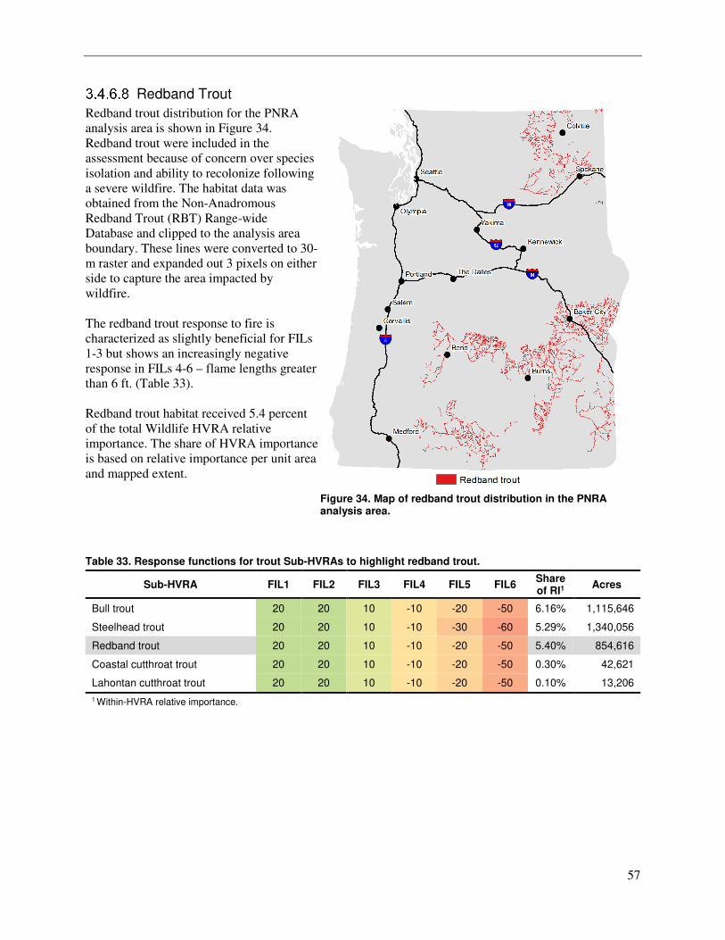
57
Redband Trout
Redband trout distribution for the PNRA
analysis area is shown in Figure 34.
Redband trout were included in the
assessment because of concern over species
isolation and ability to recolonize following
a severe wildfire. The habitat data was
obtained from the Non-Anadromous
Redband Trout (RBT) Range-wide
Database and clipped to the analysis area
boundary. These lines were converted to 30-
m raster and expanded out 3 pixels on either
side to capture the area impacted by
wildfire.
The redband trout response to fire is
characterized as slightly beneficial for FILs
1-3 but shows an increasingly negative
response in FILs 4-6 – flame lengths greater
than 6 ft. (Table 33).
Redband trout habitat received 5.4 percent
of the total Wildlife HVRA relative
importance. The share of HVRA importance
is based on relative importance per unit area
and mapped extent.
Figure 34. Map of redband trout distribution in the PNRA analysis area.
Table 33. Response functions for trout Sub-HVRAs to highlight redband trout.
Sub-HVRA FIL1 FIL2 FIL3 FIL4 FIL5 FIL6 Share of RI1
Acres
Bull trout 20 20 10 -10 -20 -50 6.16% 1,115,646
Steelhead trout 20 20 10 -10 -30 -60 5.29% 1,340,056
Redband trout 20 20 10 -10 -20 -50 5.40% 854,616
Coastal cutthroat trout 20 20 10 -10 -20 -50 0.30% 42,621
Lahontan cutthroat trout 20 20 10 -10 -20 -50 0.10% 13,206
1 Within-HVRA relative importance.
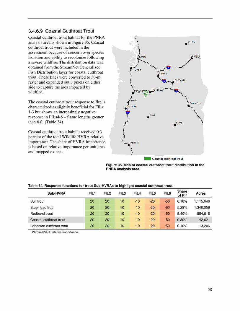
58
Coastal Cutthroat Trout
Coastal cutthroat trout habitat for the PNRA
analysis area is shown in Figure 35. Coastal
cutthroat trout were included in the
assessment because of concern over species
isolation and ability to recolonize following
a severe wildfire. The distribution data was
obtained from the StreamNet Generalized
Fish Distribution layer for coastal cutthroat
trout. These lines were converted to 30-m
raster and expanded out 3 pixels on either
side to capture the area impacted by
wildfire.
The coastal cutthroat trout response to fire is
characterized as slightly beneficial for FILs
1-3 but shows an increasingly negative
response in FILs4-6 – flame lengths greater
than 6 ft. (Table 34).
Coastal cutthroat trout habitat received 0.3
percent of the total Wildlife HVRA relative
importance. The share of HVRA importance
is based on relative importance per unit area
and mapped extent.
Figure 35. Map of coastal cutthroat trout distribution in the PNRA analysis area.
Table 34. Response functions for trout Sub-HVRAs to highlight coastal cutthroat trout.
Sub-HVRA FIL1 FIL2 FIL3 FIL4 FIL5 FIL6 Share of RI1
Acres
Bull trout 20 20 10 -10 -20 -50 6.16% 1,115,646
Steelhead trout 20 20 10 -10 -30 -60 5.29% 1,340,056
Redband trout 20 20 10 -10 -20 -50 5.40% 854,616
Coastal cutthroat trout 20 20 10 -10 -20 -50 0.30% 42,621
Lahontan cutthroat trout 20 20 10 -10 -20 -50 0.10% 13,206
1 Within-HVRA relative importance.
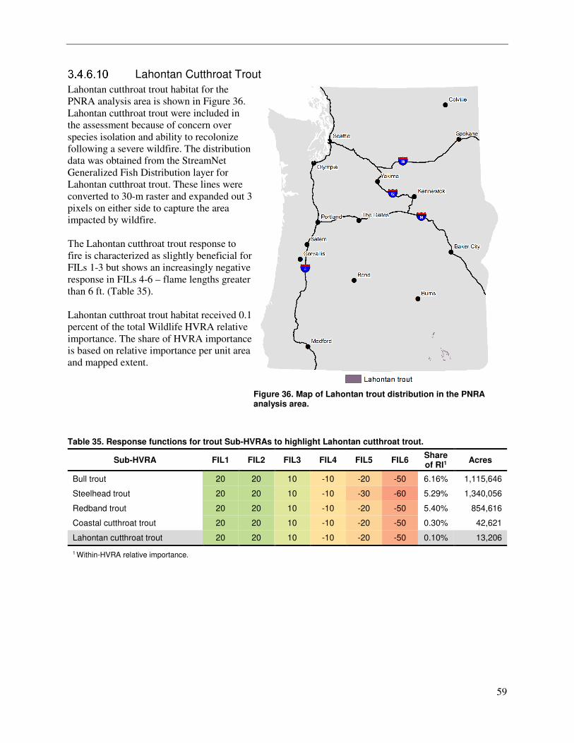
59
Lahontan Cutthroat Trout
Lahontan cutthroat trout habitat for the
PNRA analysis area is shown in Figure 36.
Lahontan cutthroat trout were included in
the assessment because of concern over
species isolation and ability to recolonize
following a severe wildfire. The distribution
data was obtained from the StreamNet
Generalized Fish Distribution layer for
Lahontan cutthroat trout. These lines were
converted to 30-m raster and expanded out 3
pixels on either side to capture the area
impacted by wildfire.
The Lahontan cutthroat trout response to
fire is characterized as slightly beneficial for
FILs 1-3 but shows an increasingly negative
response in FILs 4-6 – flame lengths greater
than 6 ft. (Table 35).
Lahontan cutthroat trout habitat received 0.1
percent of the total Wildlife HVRA relative
importance. The share of HVRA importance
is based on relative importance per unit area
and mapped extent.
Figure 36. Map of Lahontan trout distribution in the PNRA analysis area.
Table 35. Response functions for trout Sub-HVRAs to highlight Lahontan cutthroat trout.
Sub-HVRA FIL1 FIL2 FIL3 FIL4 FIL5 FIL6 Share of RI1
Acres
Bull trout 20 20 10 -10 -20 -50 6.16% 1,115,646
Steelhead trout 20 20 10 -10 -30 -60 5.29% 1,340,056
Redband trout 20 20 10 -10 -20 -50 5.40% 854,616
Coastal cutthroat trout 20 20 10 -10 -20 -50 0.30% 42,621
Lahontan cutthroat trout 20 20 10 -10 -20 -50 0.10% 13,206
1 Within-HVRA relative importance.
60
3.5 Effects Analysis Methods An effects analysis quantifies wildfire risk as the expected value of net response (Finney, 2005; Scott et
al., 2013b) also known as expected net value change (eNVC). This approach has been applied at a
national scale (Calkin et al., 2010), in regional and sub-regional assessments (Thompson et al., 2015;
Thompson et al., 2016) and several forest-level assessments of wildfire risk (Scott and Helmbrecht, 2010;
Scott et al., 2013a). Effects analysis relies on input from resource specialists to produce a tabular response
function for each HVRA occurring in the analysis area. A response function is a tabulation of the relative
change in value of an HVRA if it were to burn in each of six flame-length classes. A positive value in a
response function indicates a benefit, or increase in value; a negative value indicates a loss, or decrease in
value. Response function values ranged from -100 (greatest possible loss of resource value) to +100
(greatest possible increase in value).
Effects Analysis Calculations Integrating HVRAs with differing units of measure (for example, habitat vs. homes) requires relative
importance (RI) values for each HVRA/sub-HVRA. These values were identified in the RI workshop, as
discussed in Section 3. The final importance weight used in the risk calculations is a function of overall
HVRA importance, sub-HVRA importance, and relative extent (pixel count) of each sub-HVRA. This
value is therefore called relative importance per pixel (RIPP).
The RF and RIPP values were combined with estimates of the flame-length probability (FLP) in each of
the six flame-length classes to estimate conditional NVC (cNVC) as the sum-product of flame-length
probability (FLP) and response function value (RF) over all the six flame-length classes, with a weighting
factor adjustment for the relative importance per unit area of each HVRA, as follows:
����� ������ ∗ ���� ∗ ������
�
where i refers to flame length class (n = 6), j refers to each HVRA, and RIPP is the weighting factor based
on the relative importance and relative extent (number of pixels) of each HVRA. The cNVC calculation
shown above places each pixel of each resource on a common scale (relative importance), allowing them
to be summed across all resources to produce the total cNVC at a given pixel:
���� ��������
�
where cNVC is calculated for each pixel in the analysis area. Finally, eNVC for each pixel is calculated as
the product of cNVC and annual BP:
��� � ���� ∗ ��
61
Downscaling FSim Results for Effects Analysis FSim’s stochastic simulation approach can be computationally intensive and therefore time constraining
on large landscapes. A resulting challenge is to determine a resolution sufficiently fine to retain detail in
fuel and terrain features yet produce calibrated results in a reasonable timeframe. Moreover, HVRA are
often mapped at the same resolution as the final BP and FLPs produced by FSim. To enable greater
resolution on HVRA mapping, we chose to downscale the FSim results to 30 m, consistent with HVRA
mapping at 30 m.
We downscaled FSim results using a multi-step process. First, we resampled the original, 120-m BP and
FLP grids to 30 m. Next, we used the Focal Statistics tool in ESRI’s ArcGIS to calculate the mean BP and
FLP, of burnable pixels only, within a 7-pixel by 7-pixel moving window. Finally, we used the smoothed
BP and FLP values to “backfill” burnable pixels at 30 m that were coincident with non-burnable fuel at
120 m. The final smoothed grids resulted in original FSim values for pixels that were burnable at both
120 m and 30 m, non-zero burn probability values in burnable pixels that were non-burnable at 120 m,
and a BP of zero in non-burnable, 30-m pixels.
4 Analysis Results
4.1 Model Calibration to Historical Occurrence Due to the highly varied nature of weather and fire occurrence across the large landscape, we ran FSim
for each of the twenty-three FOAs independently, and then compiled the 23 runs into a single data
product. For each FOA, we parameterized and calibrated FSim based on the location of historical fire
ignitions within the FOA, which is consistent with how the historical record is compiled. We then used
FSim to start fires only within each FOA, but allowed those fires to spread outside of the FOA. This, too,
is consistent with how the historical record is compiled. All FOAs were calibrated to well within the 70%
confidence interval for average wildfire size and frequency. Additionally, we calibrated each FOA to
accurately mimic the distribution of wildfire sizes in the historical record to allow for future fireshed,
WUI housing risk, or other types of analyis that utilize the perimiter event set.
4.2 FSim Results FSim burn probability and flame length exceedance probability model results are presented for the PNRA
analysis area in sections 4.2.1 and 4.2.2, respectively. Additionally, all FSim results are presented in the
Deliverables folder and are described in further detail in section 6. FSim produced wildfire hazard results
for each FOA, including burn probability and conditional flame length probability. From the base FSim
outputs, flame length exceedance probabilities were calculated for each FOA. The twenty-three FOAs
were combined using the calculations described above to produce integrated maps of wildfire hazard for
the entire analysis area.
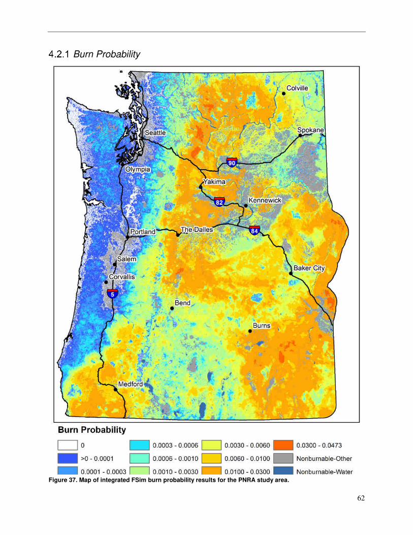
62
Burn Probability
Figure 37. Map of integrated FSim burn probability results for the PNRA study area.
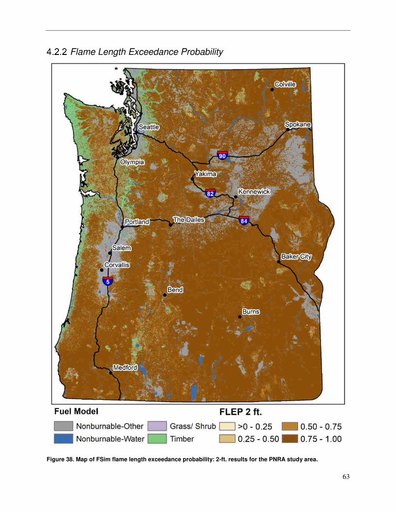
63
Flame Length Exceedance Probability
Figure 38. Map of FSim flame length exceedance probability: 2-ft. results for the PNRA study area.
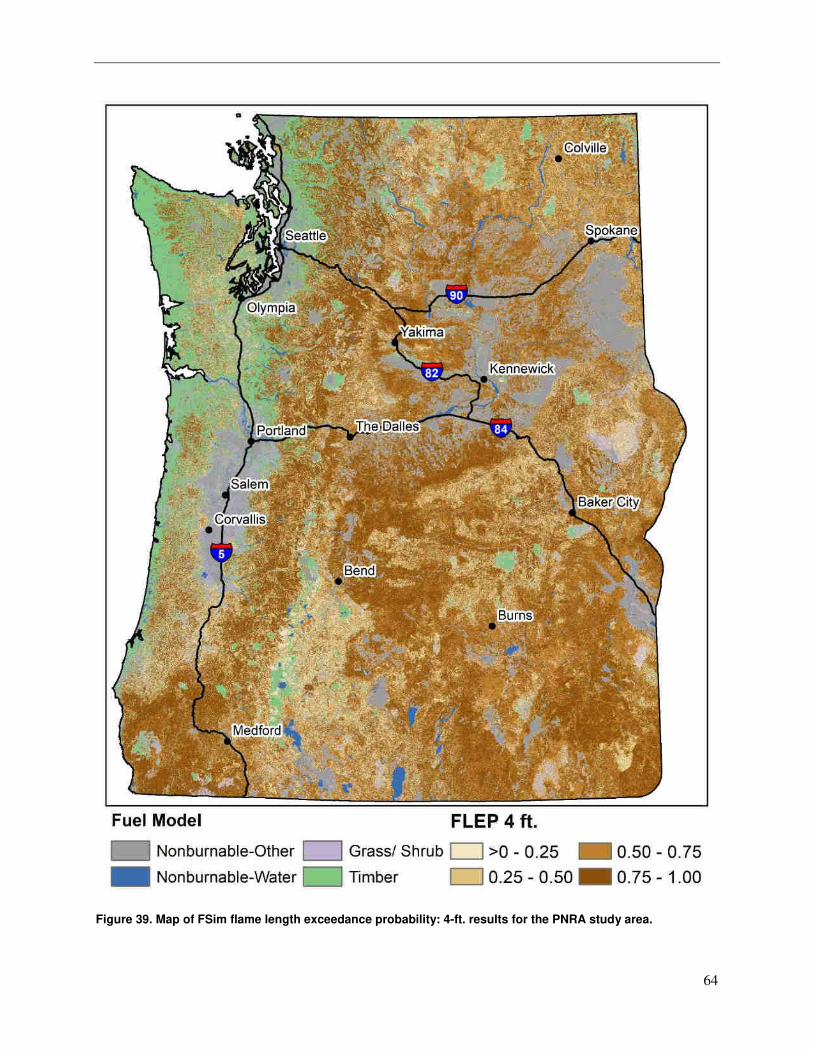
64
Figure 39. Map of FSim flame length exceedance probability: 4-ft. results for the PNRA study area.
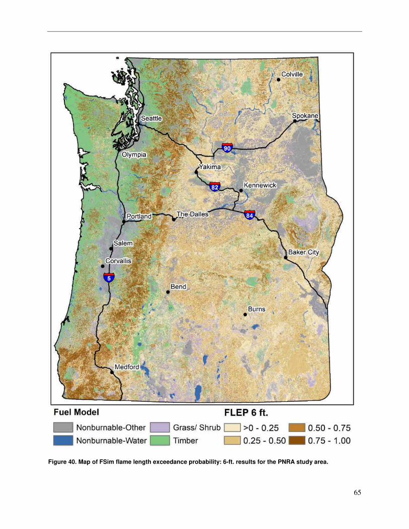
65
Figure 40. Map of FSim flame length exceedance probability: 6-ft. results for the PNRA study area.
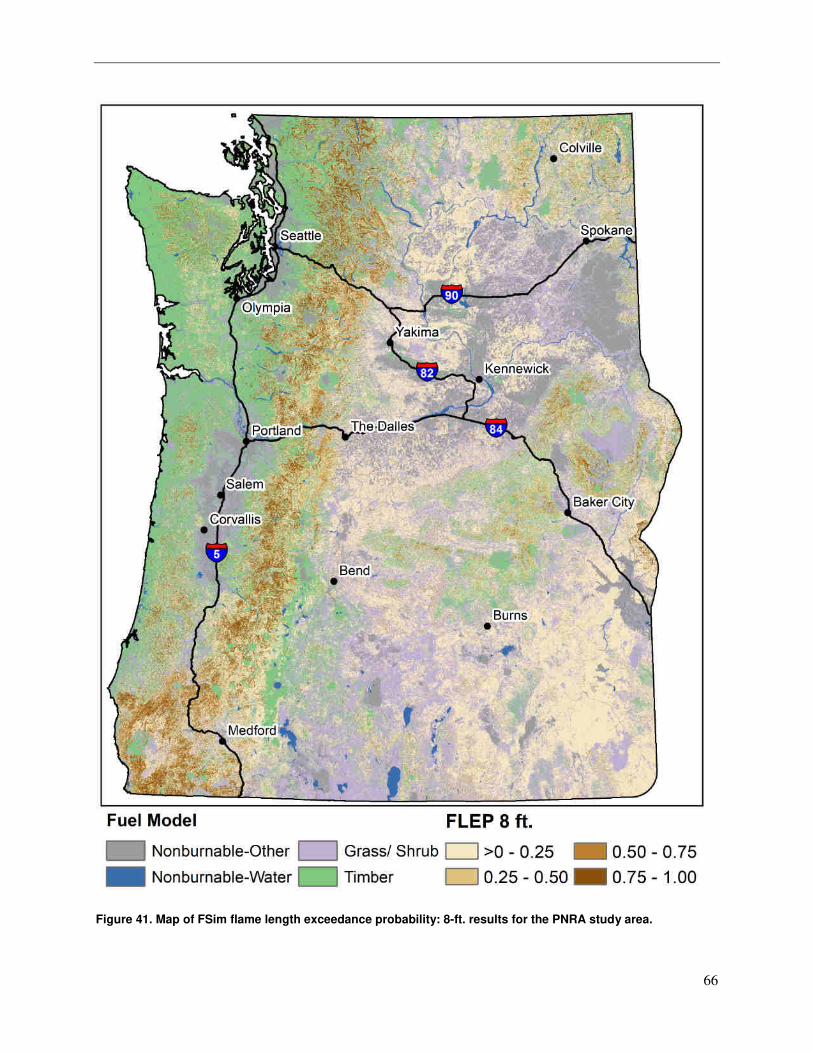
66
Figure 41. Map of FSim flame length exceedance probability: 8-ft. results for the PNRA study area.
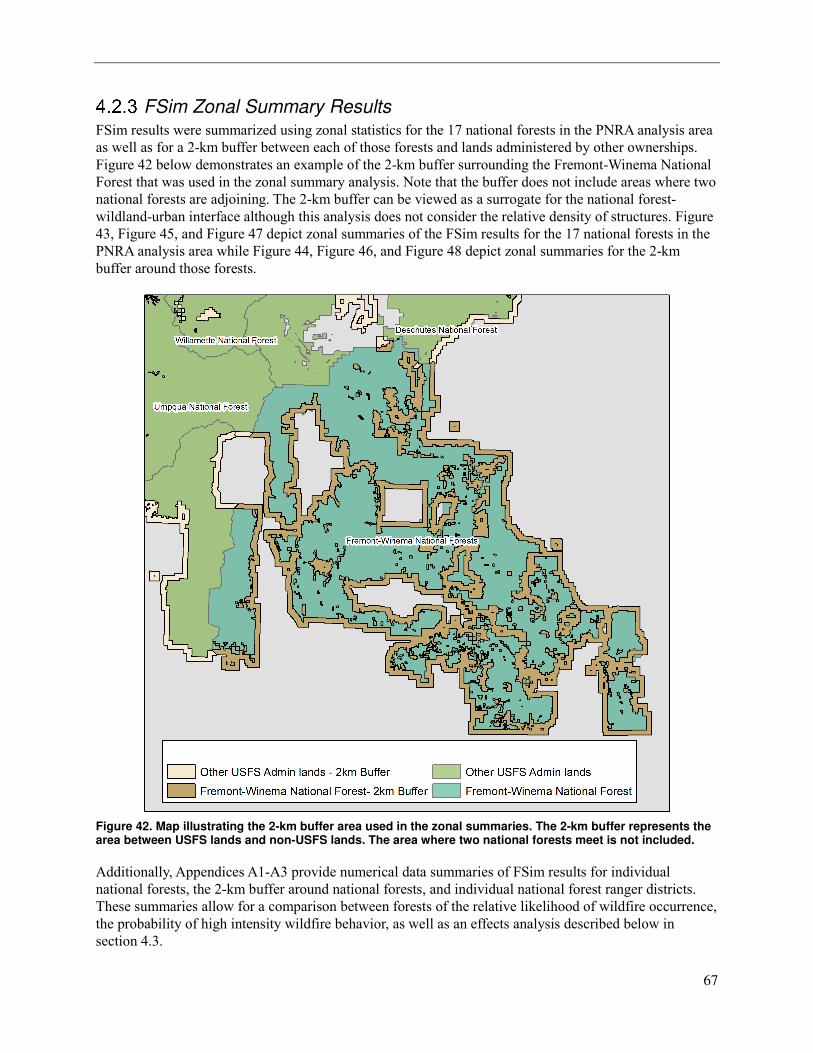
67
FSim Zonal Summary Results FSim results were summarized using zonal statistics for the 17 national forests in the PNRA analysis area
as well as for a 2-km buffer between each of those forests and lands administered by other ownerships.
Figure 42 below demonstrates an example of the 2-km buffer surrounding the Fremont-Winema National
Forest that was used in the zonal summary analysis. Note that the buffer does not include areas where two
national forests are adjoining. The 2-km buffer can be viewed as a surrogate for the national forest-
wildland-urban interface although this analysis does not consider the relative density of structures. Figure
43, Figure 45, and Figure 47 depict zonal summaries of the FSim results for the 17 national forests in the
PNRA analysis area while Figure 44, Figure 46, and Figure 48 depict zonal summaries for the 2-km
buffer around those forests.
Figure 42. Map illustrating the 2-km buffer area used in the zonal summaries. The 2-km buffer represents the area between USFS lands and non-USFS lands. The area where two national forests meet is not included.
Additionally, Appendices A1-A3 provide numerical data summaries of FSim results for individual
national forests, the 2-km buffer around national forests, and individual national forest ranger districts.
These summaries allow for a comparison between forests of the relative likelihood of wildfire occurrence,
the probability of high intensity wildfire behavior, as well as an effects analysis described below in
section 4.3.
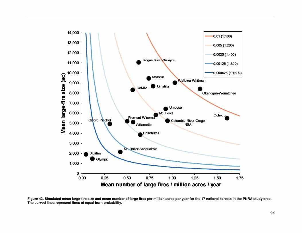
68
Figure 43. Simulated mean large-fire size and mean number of large fires per million acres per year for the 17 national forests in the PNRA study area. The curved lines represent lines of equal burn probability.
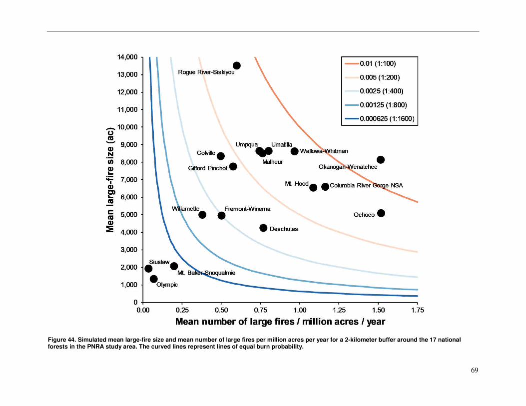
69
Figure 44. Simulated mean large-fire size and mean number of large fires per million acres per year for a 2-kilometer buffer around the 17 national forests in the PNRA study area. The curved lines represent lines of equal burn probability.
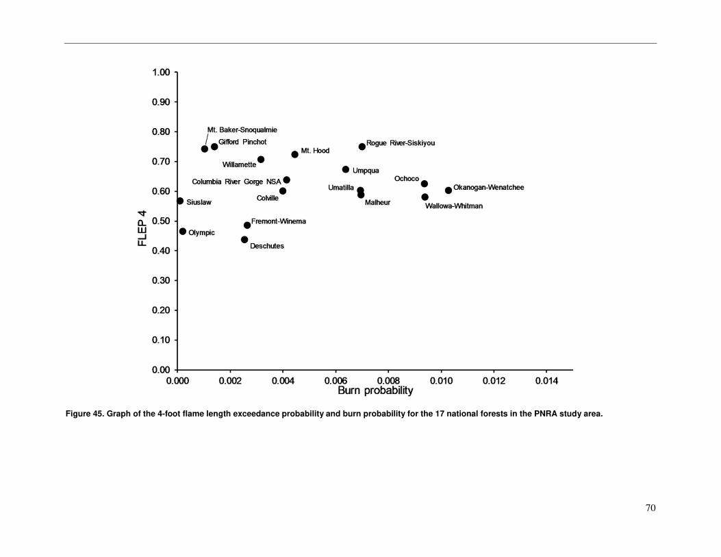
70
Figure 45. Graph of the 4-foot flame length exceedance probability and burn probability for the 17 national forests in the PNRA study area.
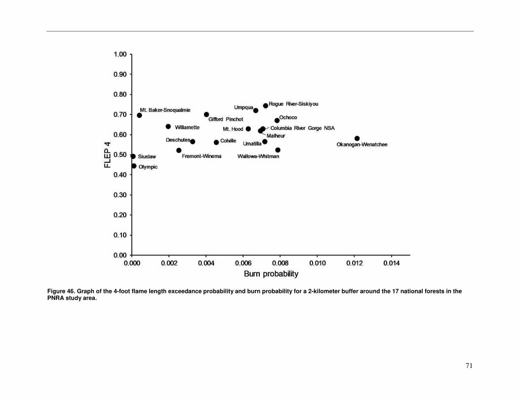
71
Figure 46. Graph of the 4-foot flame length exceedance probability and burn probability for a 2-kilometer buffer around the 17 national forests in the PNRA study area.
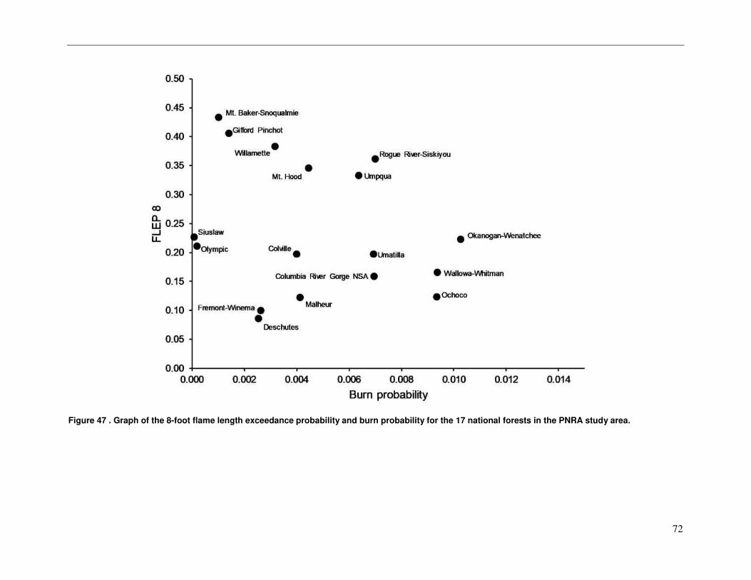
72
Figure 47 . Graph of the 8-foot flame length exceedance probability and burn probability for the 17 national forests in the PNRA study area.
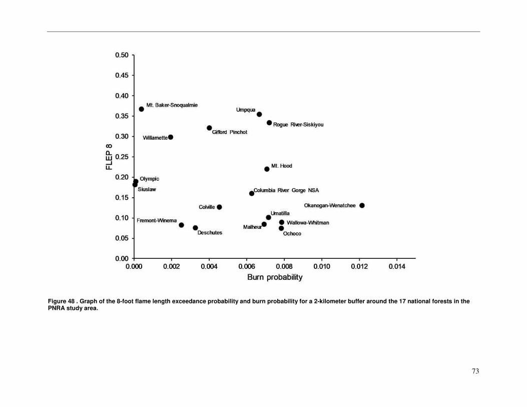
73
Figure 48 . Graph of the 8-foot flame length exceedance probability and burn probability for a 2-kilometer buffer around the 17 national forests in the PNRA study area.
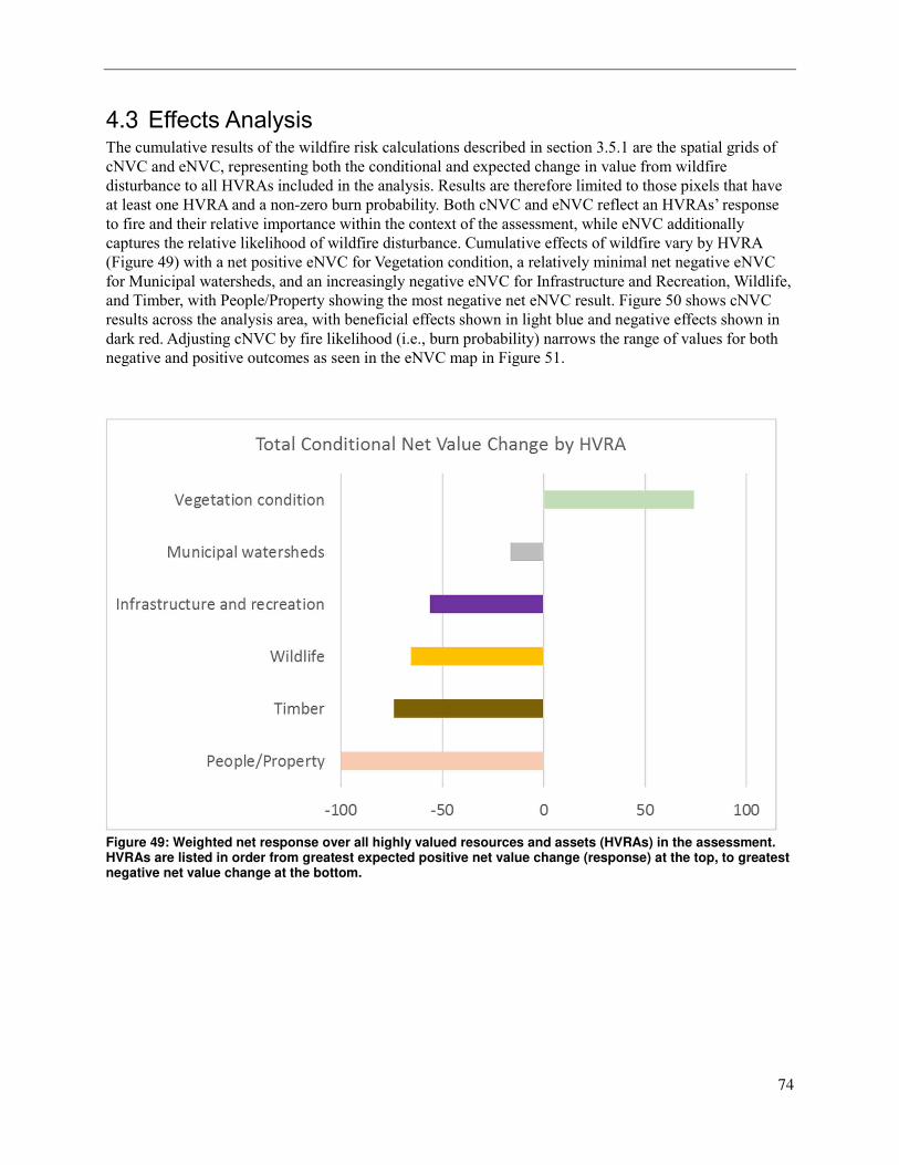
74
4.3 Effects Analysis The cumulative results of the wildfire risk calculations described in section 3.5.1 are the spatial grids of
cNVC and eNVC, representing both the conditional and expected change in value from wildfire
disturbance to all HVRAs included in the analysis. Results are therefore limited to those pixels that have
at least one HVRA and a non-zero burn probability. Both cNVC and eNVC reflect an HVRAs’ response
to fire and their relative importance within the context of the assessment, while eNVC additionally
captures the relative likelihood of wildfire disturbance. Cumulative effects of wildfire vary by HVRA
(Figure 49) with a net positive eNVC for Vegetation condition, a relatively minimal net negative eNVC
for Municipal watersheds, and an increasingly negative eNVC for Infrastructure and Recreation, Wildlife,
and Timber, with People/Property showing the most negative net eNVC result. Figure 50 shows cNVC
results across the analysis area, with beneficial effects shown in light blue and negative effects shown in
dark red. Adjusting cNVC by fire likelihood (i.e., burn probability) narrows the range of values for both
negative and positive outcomes as seen in the eNVC map in Figure 51.
Figure 49: Weighted net response over all highly valued resources and assets (HVRAs) in the assessment. HVRAs are listed in order from greatest expected positive net value change (response) at the top, to greatest negative net value change at the bottom.
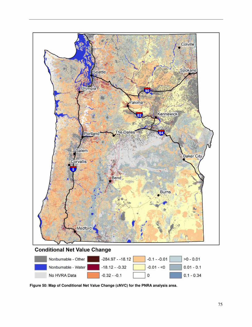
75
Figure 50: Map of Conditional Net Value Change (cNVC) for the PNRA analysis area.
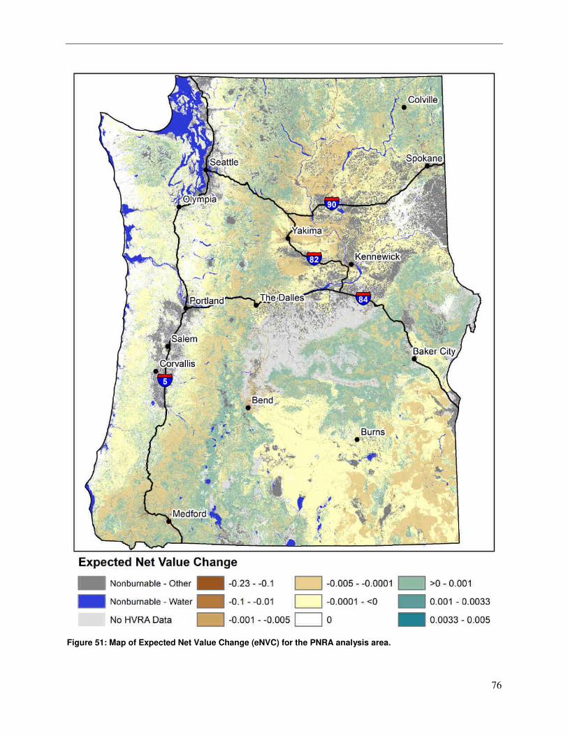
76
Figure 51: Map of Expected Net Value Change (eNVC) for the PNRA analysis area.
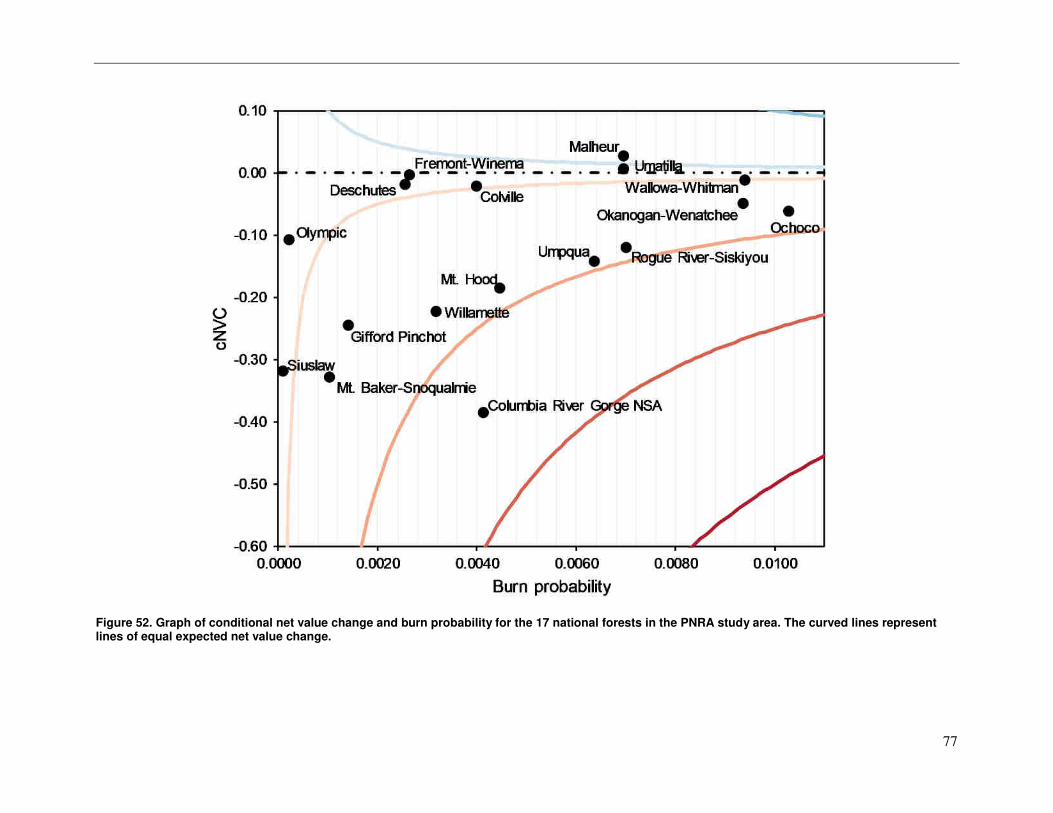
77
Figure 52. Graph of conditional net value change and burn probability for the 17 national forests in the PNRA study area. The curved lines represent lines of equal expected net value change.
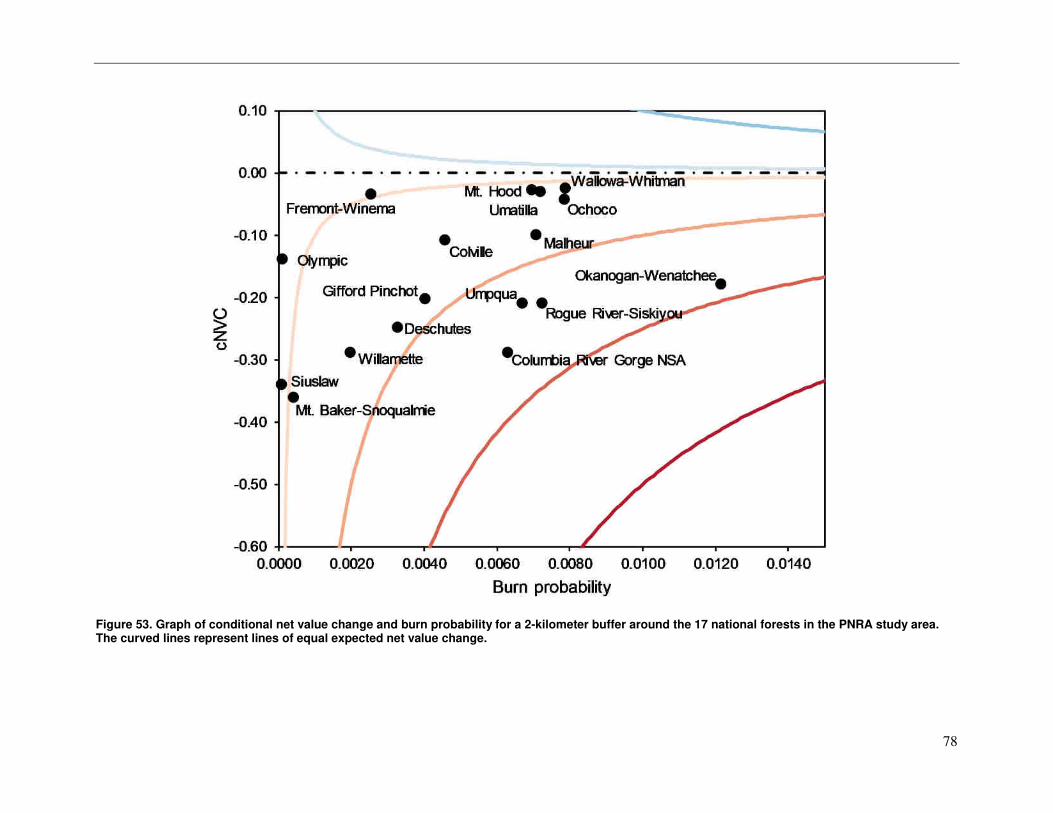
78
Figure 53. Graph of conditional net value change and burn probability for a 2-kilometer buffer around the 17 national forests in the PNRA study area. The curved lines represent lines of equal expected net value change.
79
5 Analysis Summary The Pacific Northwest QWRA provides foundational information about wildfire hazard and risk to highly
valued resources and assets across the Region. The results represent the best available science across a
range of disciplines. While this report was generated by Pyrologix LLC, the overall analysis was
developed as a collaborative effort with numerous USFS, BLM, TNC, ODF, and WA DNR, Fire/Fuels
Planners, Resource Specialists, Wildlife Biologists, Geospatial Analysts, and Information Specialists. This
analysis can provide great utility in a range of applications including: resource planning, prioritization and
implementation of prevention and mitigation activities and wildfire incident response planning. Lastly,
this analysis should be viewed as a living document. While the effort to parameterize and to calibrate
model inputs should remain static, the landscape file should be periodically revisited and updated to
account for future forest disturbances. Additionally, the HVRA mapping may also need to be updated to
account for forthcoming resource challenges and needs within the geographic area.
80
6 Data Dictionary • FSim modeling results are presented in three geodatabases:
• PNRA_120m_V3_Final.gdb – Mosaic FSim results for the twenty-three FOAs in the PNRA
project area.
• PNRA_rfV3_AllPerims.gdb – Event set outputs from FSim that includes all simulated wildfire
perimeters.
• PNRA_rfV3_AllIgnitions.gdb – Event set outputs from FSim that include the start location of
all simulated wildfire perimeters.
1. PNRA_120m_V3_Final.gdb – This geodatabase contains 13 rasters representing mosaic data results
from the FSim simulations in the 23 FOAs within the PNRA project area:
a. FLEP_2 –
This dataset represents the conditional probability of exceeding a nominal flame-length
value (also known as flame-length exceedance probability, or FLEP). There are five FLEP
rasters. FLEP_GT2 is the conditional probability of exceeding a flame length of 2 feet; it is
calculated as the sum of iFLP_FIL2 through iFLP_FIL6. FLEP_GT4 is the conditional
probability of exceeding a flame length of 4 feet; it is calculated as the sum of iFLP_FIL3
through iFLP_FIL6. FLEP_GT6 is the conditional probability of exceeding a flame length of
6 feet; it is calculated as the sum of iFLP_FIL4 through iFLP_FIL6. FLEP_GT8 is the
conditional probability of exceeding a flame length of 8 feet; it is calculated as the sum of
iFLP_FIL5 and iFLP_FIL6. There is no raster for FLEP_GT0 because, by definition, for all
burnable pixels there is a 100 percent probability that flame length will exceed 0, given that a
fire occurs.
The iFLP_FILx rasters are the integrated (project wide) conditional probabilities of
observing flame length in each of six classes: iFLP_FIL1 represents flame lengths from 0 - 2
ft., iFLP_FIL2 represents flame lengths from 2 - 4 ft., iFLP_FIL3 represents flame lengths
from 4 - 6 ft., iFLP_FIL4 represents flame lengths from 6 - 8 ft., iFLP_FIL5 represents flame
lengths from 8 - 12 ft., and iFLP_FIL6 represents flame lengths >12 ft.
b. FLEP_4 – see FLEP_2 description above
c. FLEP_6 – see FLEP_2 description above
d. FLEP_8 – see FLEP_2 description above
e. iBP –
This dataset is a 120-m cell size raster representing annual burn probability across the
project area. The individual-FOA BPs were integrated into this overall result for the project
area using a natural-weighting method that Pyrologix developed on an earlier project and
subsequently published (Thompson and others 2013; “Assessing Watershed-Wildfire Risks
on National Forest System Lands in the Rocky Mountain Region of the United States”). With
this method, BP values for pixels well within the boundary of a FOA are influenced only by
that FOA. Near the border with another FOA the results are influenced by that adjacent FOA.
The weighting of each FOA is in proportion to its contribution to the overall BP at each pixel.
f. iCFL –
This dataset is a 120-m cell size raster representing the mean conditional flame length
(given that a fire occurs). It is a measure of the central tendency of flame length. This raster
was calculated as the sum-product of iFLP_FILx and the midpoint flame length of each of the
six iFLP_FILs. For iFLP_FIL6, for which there is no midpoint, we used a surrogate flame
length of 100 feet (representing torching trees).
81
g. iFLP_FIL1 –
This dataset is a 120-m cell size raster representing the mean conditional flame length
(given that a fire occurs). This is also called the flame-length probability (FLP) and is a
measure of the central tendency of flame length. This raster was calculated as the sum-
product of the probability at each flame-length class and the midpoint flame length value of
each of the six FILs. For FIL6, for which there is no midpoint, we used a surrogate flame
length of 100 feet (representing torching trees) in timber fuel models and a flame length of 20
feet in all in grass, grass-shrub and shrub fuel types.
The individual-FOA iFLP_FILx rasters were integrated into this overall result for the
project area using a natural-weighting method that Pyrologix developed on an earlier project
and subsequently published (Thompson and others 2013; “Assessing Watershed-Wildfire
Risks on National Forest System Lands in the Rocky Mountain Region of the United States”).
With this method, the iFLP_FILx values for pixels well within the boundary of a FOA are
influenced only by that FOA. Near the border with another FOA the results are also
influenced by that adjacent FOA. The weighting of each FOA is in proportion to its
contribution to the overall BP at each pixel.
h. iFLP_FIL2 – see iFLP_FIL1 description above
i. iFLP_FIL3 – see iFLP_FIL1 description above
j. iFLP_FIL4 – see iFLP_FIL1 description above
k. iFLP_FIL5 – see iFLP_FIL1 description above
l. iFLP_FIL6 – see iFLP_FIL1 description above
m. iMFI –
This dataset is a 120-m cell size raster representing the mean conditional fireline intensity
(kW/m) given that a fire occurs. It is a measure of the central tendency of fireline intensity.
The individual-FOA MFI rasters were integrated into this overall result for the project area
using a natural-weighting method that Pyrologix developed on an earlier project and
subsequently published (Thompson and others 2013; “Assessing Watershed-Wildfire Risks
on National Forest System Lands in the Rocky Mountain Region of the United States”). With
this method, the iMFI values for pixels well within the boundary of a FOA are influenced
only by that FOA. Near the border with another FOA the results are also influenced by that
adjacent FOA. The weighting of each FOA is in proportion to its contribution to the overall
BP at each pixel.
2. PNRA_rfV3_AllPerims.gdb – This dataset represents the simulated wildfire perimeters within each
of the twenty-three Fire Occurrence Areas (FOA) that comprise the PNRA project area. Each _Perims
feature class includes an attribute table with the following attributes:
a. FIRE_NUMBE - the unique fire number for a simulation
b. THREAD_NUM - the thread number that simulated the fire (the number of threads is
determined by the number of CPUs in the workstation, the number of processing cores per
CPU, and whether the cores are hyperthreaded.)
c. ERC_STARTD - the ERC(G) value on the start day of the fire
d. ERC_PERCEN - the ERC(G) percentile associated with ERC_STARTD. The
ERC_PERCEN is a simple lookup from the ERC_STARTD from the "percentiles" section of
the .frisk file.
e. NUM_BURNDA - the number of days the fire burned during the simulation. This does not
include any no-burn days (days below the 80th percentile ERC
f. START_DAY - the Julian day of the fire start
82
g. YEAR - the iteration number (year) for which the fire was simulated
h. Xcoord/Ycoord - the coordinates of the fire's ignition point
i. CONTAIN - the reason for the cessation of fire growth on the simulated fire
j. FOA – the FOA number where the ignition is located
k. UNQ_ID – concatenation of FOA number and FIRE_NUMBE
l. NumIterations – the number of iterations within a simulation. Individual FOAs were run
with 10,000 iterations. When generating additional analytical products from the FSim event
set, results must be weighted by iteration number to avoid introducing error
m. GIS_SizeAc – the final wildfire size (acres) generated as an ArcGIS calculation based on
feature geometry
n. GIS_SizeHa – the final wildfire size (hectares) generated as an ArcGIS calculation based on
feature geometry
o. FSim_SizeAc - is the final fire size (acres) generated within FSim based on raster count.
Best-practice is to calculate GIS acres for each perimeter instead of relying on SizeAc,
especially if subsequent analyses will be based on GIS acres
p. NumParts – Number of geometry parts in the simulated wildfire perimeter
q. ContainsIgn – True/False value (1,0) that describes if the location of the ignition point is
contained within the simulated wildfire perimeter polygon. The ignition may not be included
within the simulated perimeter due to how FSIM converts pixel geometry to polygon
geometry or as a result of a post processing script that removed small artifacts generated from
the FSim trimming suppression algorithm.
3. PNRA_rfV3_AllIgnitions.gdb – This dataset represents the simulated fire start locations within each
of the twenty-three Fire Occurrence Areas (FOA) that comprise the PNRA project area. Each
_AllIgnitions feature class includes an attribute table with the following attributes:
a. FIRE_NUMBE - the unique fire number for a simulation
b. THREAD_NUM - the thread number that simulated the fire (the number of threads is
determined by the number of CPUs in the workstation, the number of processing cores per
CPU, and whether the cores are hyperthreaded.)
c. ERC_STARTD - the ERC(G) value on the start day of the fire
d. ERC_PERCEN - the ERC(G) percentile associated with ERC_STARTD. The
ERC_PERCEN is a simple lookup from the ERC_STARTD from the "percentiles" section of
the .frisk file.
e. NUM_BURNDA - the number of days the fire burned during the simulation. This does not
include any no-burn days (days below the 80th percentile ERC
f. START_DAY - the Julian day of the fire start
g. YEAR - the iteration number (year) for which the fire was simulated
h. Xcoord/Ycoord - the coordinates of the fire's ignition point
i. CONTAIN - the reason for the cessation of fire growth on the simulated fire
j. FOA – the FOA number where the ignition is located
k. UNQ_ID – concatenation of FOA number and FIRE_NUMBE
l. NumIterations – the number of iterations within a simulation. Individual FOAs were run
with 10,000 iterations. When generating additional analytical products from the FSim event
set, results must be weighted by iteration number to avoid introducing error
m. GIS_SizeAc – the final wildfire size (acres) generated as an ArcGIS calculation based on
feature geometry
n. GIS_SizeHa – the final wildfire size (hectares) generated as an ArcGIS calculation based on
feature geometry
83
o. FSim_SizeAc - is the final fire size (acres) generated within FSim based on raster count.
Best-practice is to calculate GIS acres for each perimeter instead of relying on SizeAc,
especially if subsequent analyses will be based on GIS acres
p. NumParts – Number of geometry parts in the simulated wildfire perimeter
q. ContainsIgn – True/False value (1,0) that describes if the location of the ignition point is
contained within the simulated wildfire perimeter polygon. The ignition may not be included
within the simulated perimeter due to how FSim converts pixel geometry to polygon
geometry or as a result of a post processing script that removed small artifacts generated from
the FSim trimming suppression algorithm.
84
7 References Buckley, M., Beck, N., Bowden, P., Miller, M.E., Hill, B., Luce, C., Elliott, W.J., Enstice, N., Podolak,
K., Winford, E., Smith, S.L., Bokach, M., Reichert, M., Edelson, D., Gaither, J., 2014.
Mokelumne watershed avoided cost analysis: why Siera fuel treatments make economic sense. In.
The Nature Conservancy, and U.S. Department of Agriculture, Forest Service. Sierra Nevada
Conservancy, Auburn, California.
Calkin, D., Ager, A., Gilbertson-Day, J., 2010. Wildfire Risk and Hazard: procedures for the first
approximation. In, Gen. Tech. Rep. U.S. Department of Agriculture, Forest Service, Rocky
Mountain Research Station, Fort Collins, CO, p. 62.
DeMeo, T., Haugo, R., Ringo, C., In Press. Expanding Our Understanding of Forest Structural
Restoration Needs in the Pacific Northwest, USA. Northwest Science.
Finney, M.A., 2005. The challenge of quantitative risk analysis for wildland fire. Forest Ecology and
Management 211, 97-108.
Finney, M.A., McHugh, C., Grenfel, I.C., Riley, K.L., Short, K.C., 2011. A simulation of probabilistic
wildfire risk components for the continental United States. Stochastic Environmental Research
and Risk Assessment 25.7, 973-1000.
Glenn, E.M., Lesmeister, D.B., Davis, R.J., Hollen, B., Poopatanapong, A., 2017. Estimating density of a
territorial species in a dynamic landscape. Landscape Ecology 32, 563-579.
Jolly, M., 2014. Personal Communication. In, U.S. Forest Service: Missoula, MT, USA.
NFDRS, 2002. Gaining a basic understanding of the National Fire Danger Rating System.
Ringo, C., Ager, A.A., Day, M.A., Crim, S., 2016. A spatial database for restoration management
capability on national forests in the Pacific Northwest USA. General Technical Report-Pacific
Northwest Research Station, USDA Forest Service.
Scott, J.H., 2006. An Analytical Framework for Quantifying Wildland Fire Risk and Fuel Treatment
Benefit. USDA Forest Service Proceedings RMRS-P-41.
Scott, J.H., Helmbrecht, D., 2010. Wildfire threat to key resources on the Beaverhead-Deerlodge National
Forest. In, Unpublished report, p. 44.
Scott, J.H., Helmbrecht, D., Williamson, M., 2013a. Response of highly valued resources and assets to
wildfire within Grand Teton National Park and the Bridger-Teton National Forest. In,
Unpublished report, p. 71.
Scott, J.H., Thompson, M.P., Calkin, D.E., 2013b. A wildfire risk assessment framework for land and
resource management. In, General Technical Report. U.S. Department of Agriculture, Forest
Service, Rocky Mountain Research Station, Fort Collins, CO, p. 92.
Short, K.C., 2017. Spatial wildfire occurrence data for the United States, 1992-2015
[FPA_FOD_20170508]. In. Forest Service Research Data Archive, Fort Collins, CO.
Thompson, M.P., Bowden, P., Brough, A., Scott, J.H., Gilbertson-Day, J., Taylor, A.H., Anderson, J.,
Haas, J., 2016. Application of wildfire risk assessment results to wildfire response planning in the
Southern Sierra Nevada, California, USA. Forests 7, 64.
Thompson, M.P., Haas, J., Gilbertson-Day, J., Scott, J.H., Langowski, P., Bowne, E., Calkin, D.E., 2015.
Development and application of a geospatial wildfire exposure and risk calculation tool.
Environmental Modelling & Software 63, 61-72.
Thompson, M.P., Scott, J., Langowski, P.G., Gilbertson-Day, J.W., Haas, J.R., Bowne, E.M., 2013a.
Assessing watershed-wildfire risks on national forest system lands in the rocky mountain region
of the United States. Water 5, 945-971.
Thompson, M.P., Scott, J.H., Helmbrecht, D., Calkin, D.E., 2013b. Integrated wildfire risk assessment:
Framework development and application on the Lewis and Clark National Forest in Montana,
USA. Integrated environmental assessment and management 9, 329-342.
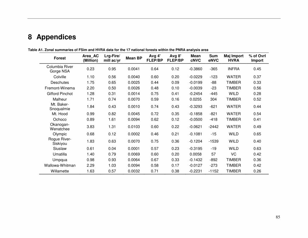
85
8 Appendices
Table A1. Zonal summaries of FSim and HVRA data for the 17 national forests within the PNRA analysis area
Forest Area_AC (Million)
Lrg-Fire/ mill ac/yr
Mean BP Avg 4'
FLEP/BP Avg 8'
FLEP/BP Mean cNVC
Sum eNVC
Maj Import HVRA
% of Ovrl Import
Columbia River Gorge NSA
0.23 0.95 0.0041 0.64 0.12 -0.3860 -365 INFRA 0.45
Colville 1.10 0.56 0.0040 0.60 0.20 -0.0229 -123 WATER 0.37
Deschutes 1.75 0.65 0.0025 0.44 0.09 -0.0199 -88 TIMBER 0.33
Fremont-Winema 2.20 0.50 0.0026 0.48 0.10 -0.0039 -23 TIMBER 0.56
Gifford Pinchot 1.28 0.31 0.0014 0.75 0.41 -0.2454 -445 WILD 0.28
Malheur 1.71 0.74 0.0070 0.59 0.16 0.0255 304 TIMBER 0.52
Mt. Baker-Snoqualmie
1.84 0.43 0.0010 0.74 0.43 -0.3293 -621 WATER 0.44
Mt. Hood 0.99 0.82 0.0045 0.72 0.35 -0.1858 -821 WATER 0.54
Ochoco 0.89 1.61 0.0094 0.62 0.12 -0.0500 -418 TIMBER 0.41
Okanogan-Wenatchee
3.83 1.31 0.0103 0.60 0.22 -0.0621 -2442 WATER 0.49
Olympic 0.68 0.12 0.0002 0.46 0.21 -0.1081 -15 WILD 0.65
Rogue River-Siskiyou
1.83 0.63 0.0070 0.75 0.36 -0.1204 -1539 WILD 0.40
Siuslaw 0.61 0.04 0.0001 0.57 0.23 -0.3195 -19 WILD 0.63
Umatilla 1.40 0.79 0.0069 0.60 0.20 0.0058 57 VC 0.42
Umpqua 0.98 0.93 0.0064 0.67 0.33 -0.1432 -892 TIMBER 0.36
Wallowa-Whitman 2.29 1.03 0.0094 0.58 0.17 -0.0127 -273 TIMBER 0.42
Willamette 1.63 0.57 0.0032 0.71 0.38 -0.2231 -1152 TIMBER 0.26
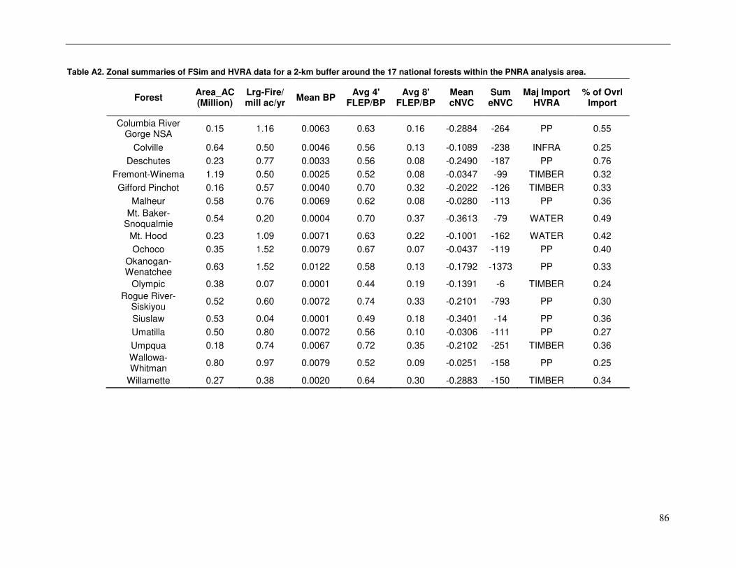
86
Table A2. Zonal summaries of FSim and HVRA data for a 2-km buffer around the 17 national forests within the PNRA analysis area.
Forest Area_AC (Million)
Lrg-Fire/ mill ac/yr
Mean BP Avg 4'
FLEP/BP Avg 8'
FLEP/BP Mean cNVC
Sum eNVC
Maj Import HVRA
% of Ovrl Import
Columbia River Gorge NSA
0.15 1.16 0.0063 0.63 0.16 -0.2884 -264 PP 0.55
Colville 0.64 0.50 0.0046 0.56 0.13 -0.1089 -238 INFRA 0.25
Deschutes 0.23 0.77 0.0033 0.56 0.08 -0.2490 -187 PP 0.76
Fremont-Winema 1.19 0.50 0.0025 0.52 0.08 -0.0347 -99 TIMBER 0.32
Gifford Pinchot 0.16 0.57 0.0040 0.70 0.32 -0.2022 -126 TIMBER 0.33
Malheur 0.58 0.76 0.0069 0.62 0.08 -0.0280 -113 PP 0.36
Mt. Baker-Snoqualmie
0.54 0.20 0.0004 0.70 0.37 -0.3613 -79 WATER 0.49
Mt. Hood 0.23 1.09 0.0071 0.63 0.22 -0.1001 -162 WATER 0.42
Ochoco 0.35 1.52 0.0079 0.67 0.07 -0.0437 -119 PP 0.40
Okanogan-Wenatchee
0.63 1.52 0.0122 0.58 0.13 -0.1792 -1373 PP 0.33
Olympic 0.38 0.07 0.0001 0.44 0.19 -0.1391 -6 TIMBER 0.24
Rogue River-Siskiyou
0.52 0.60 0.0072 0.74 0.33 -0.2101 -793 PP 0.30
Siuslaw 0.53 0.04 0.0001 0.49 0.18 -0.3401 -14 PP 0.36
Umatilla 0.50 0.80 0.0072 0.56 0.10 -0.0306 -111 PP 0.27
Umpqua 0.18 0.74 0.0067 0.72 0.35 -0.2102 -251 TIMBER 0.36
Wallowa-Whitman
0.80 0.97 0.0079 0.52 0.09 -0.0251 -158 PP 0.25
Willamette 0.27 0.38 0.0020 0.64 0.30 -0.2883 -150 TIMBER 0.34
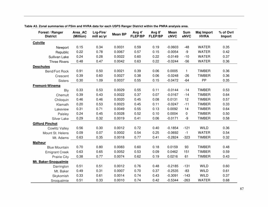
87
Table A3. Zonal summaries of FSim and HVRA data for each USFS Ranger District within the PNRA analysis area.
Forest / Ranger District
Area_AC (Million)
Lrg-Fire/ mill ac/yr
Mean BP Avg 4'
FLEP/BP Avg 8'
FLEP/BP Mean cNVC
Sum eNVC
Maj Import HVRA
% of Ovrl Import
Colville
Newport 0.15 0.34 0.0031 0.59 0.19 -0.0603 -48 WATER 0.35
Republic 0.22 0.78 0.0067 0.57 0.15 -0.0054 -9 WATER 0.42
Sullivan Lake 0.24 0.28 0.0022 0.60 0.22 -0.0149 -10 WATER 0.37
Three Rivers 0.48 0.47 0.0042 0.63 0.22 -0.0244 -56 WATER 0.36
Deschutes
Bend/Fort Rock 0.91 0.50 0.0021 0.39 0.06 0.0005 1 TIMBER 0.36
Crescent 0.39 0.60 0.0027 0.38 0.06 -0.0248 -26 TIMBER 0.36
Sisters 0.30 1.09 0.0037 0.55 0.15 -0.0472 -64 PP 0.35
Fremont-Winema
Bly 0.33 0.53 0.0029 0.55 0.11 -0.0144 -14 TIMBER 0.53
Chemult 0.39 0.43 0.0022 0.37 0.07 -0.0167 -14 TIMBER 0.64
Chiloquin 0.46 0.46 0.0020 0.45 0.08 0.0131 12 TIMBER 0.57
Klamath 0.20 0.53 0.0023 0.45 0.11 -0.0247 -11 TIMBER 0.33
Lakeview 0.31 0.71 0.0049 0.55 0.13 0.0092 14 TIMBER 0.64
Paisley 0.24 0.45 0.0028 0.52 0.10 0.0004 0 TIMBER 0.50
Silver Lake 0.29 0.32 0.0019 0.41 0.06 -0.0171 -9 TIMBER 0.58
Gifford Pinchot
Cowlitz Valley 0.56 0.30 0.0012 0.72 0.40 -0.1854 -121 WILD 0.36
Mount St. Helens 0.09 0.07 0.0002 0.54 0.25 -0.0692 -1 WATER 0.54
Mt. Adams 0.63 0.35 0.0018 0.77 0.41 -0.2824 -323 TIMBER 0.32
Malheur
Blue Mountain 0.70 0.80 0.0083 0.60 0.18 0.0159 93 TIMBER 0.48
Emigrant Creek 0.63 0.65 0.0052 0.53 0.09 0.0462 151 TIMBER 0.59
Prairie City 0.38 0.77 0.0074 0.62 0.19 0.0216 61 TIMBER 0.43
Mt. Baker-Snoqualmie
Darrington 0.51 0.51 0.0012 0.76 0.48 -0.2185 -131 WILD 0.60
Mt. Baker 0.49 0.31 0.0007 0.70 0.37 -0.2535 -83 WILD 0.61
Skykomish 0.33 0.61 0.0014 0.74 0.43 -0.3091 -143 WILD 0.37
Snoqualmie 0.51 0.33 0.0010 0.74 0.42 -0.5344 -263 WATER 0.68
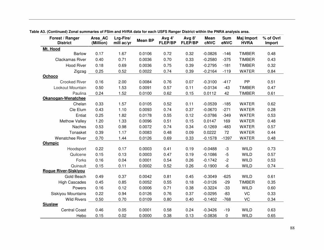
88
Table A3. (Continued) Zonal summaries of FSim and HVRA data for each USFS Ranger District within the PNRA analysis area.
Forest / Ranger District
Area_AC (Million)
Lrg-Fire/ mill ac/yr
Mean BP Avg 4'
FLEP/BP Avg 8'
FLEP/BP Mean cNVC
Sum eNVC
Maj Import HVRA
% of Ovrl Import
Mt. Hood Barlow 0.17 1.67 0.0106 0.72 0.32 -0.0826 -146 TIMBER 0.48
Clackamas River 0.40 0.71 0.0036 0.70 0.33 -0.2580 -375 TIMBER 0.43
Hood River 0.18 0.69 0.0036 0.75 0.39 -0.2795 -181 TIMBER 0.32
Zigzag 0.25 0.52 0.0022 0.74 0.39 -0.2164 -119 WATER 0.84
Ochoco Crooked River 0.16 2.00 0.0084 0.76 0.07 -0.3100 -417 PP 0.51
Lookout Mountain 0.50 1.53 0.0091 0.57 0.11 -0.0134 -43 TIMBER 0.47
Paulina 0.24 1.52 0.0100 0.62 0.15 0.0112 42 TIMBER 0.61
Okanogan-Wenatchee Chelan 0.33 1.57 0.0105 0.52 0.11 -0.0539 -185 WATER 0.62
Cle Elum 0.43 1.10 0.0093 0.74 0.37 -0.0670 -271 WATER 0.28
Entiat 0.25 1.82 0.0178 0.55 0.12 -0.0786 -349 WATER 0.53
Methow Valley 1.20 1.33 0.0096 0.51 0.15 0.0147 169 WATER 0.48
Naches 0.53 0.98 0.0072 0.74 0.34 -0.1269 -483 WATER 0.57
Tonasket 0.39 1.17 0.0083 0.48 0.09 0.0222 72 WATER 0.44
Wenatchee River 0.70 1.44 0.0126 0.69 0.33 -0.1578 -1397 WATER 0.48
Olympic Hoodsport 0.22 0.17 0.0003 0.41 0.19 -0.0488 -3 WILD 0.73
Quilcene 0.15 0.13 0.0003 0.47 0.19 -0.1086 -5 WILD 0.57
Forks 0.16 0.04 0.0001 0.54 0.26 -0.1742 -2 WILD 0.53
Quinault 0.15 0.11 0.0002 0.52 0.26 -0.1900 -6 WILD 0.74
Rogue River-Siskiyou Gold Beach 0.49 0.37 0.0042 0.81 0.45 -0.3049 -625 WILD 0.61
High Cascades 0.45 0.85 0.0052 0.55 0.18 -0.0126 -29 TIMBER 0.35
Powers 0.16 0.12 0.0006 0.71 0.38 -0.3224 -33 WILD 0.60
Siskiyou Mountains 0.22 0.94 0.0126 0.76 0.37 -0.0295 -83 VC 0.33
Wild Rivers 0.50 0.70 0.0109 0.80 0.40 -0.1402 -768 VC 0.34
Siuslaw Central Coast 0.46 0.05 0.0001 0.58 0.24 -0.3426 -19 WILD 0.63
Hebo 0.15 0.02 0.0000 0.38 0.13 -0.0836 0 WILD 0.65
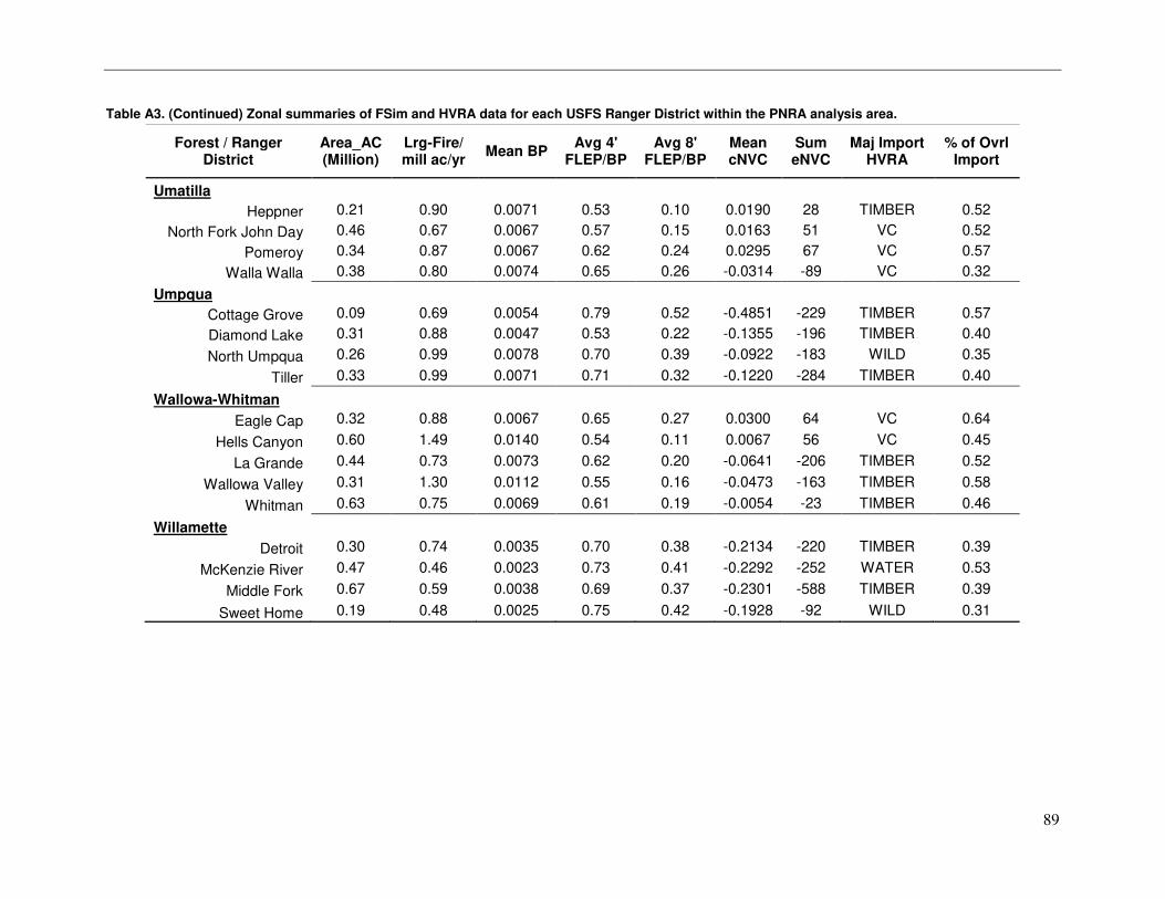
89
Table A3. (Continued) Zonal summaries of FSim and HVRA data for each USFS Ranger District within the PNRA analysis area.
Forest / Ranger District
Area_AC (Million)
Lrg-Fire/ mill ac/yr
Mean BP Avg 4'
FLEP/BP Avg 8'
FLEP/BP Mean cNVC
Sum eNVC
Maj Import HVRA
% of Ovrl Import
Umatilla
Heppner 0.21 0.90 0.0071 0.53 0.10 0.0190 28 TIMBER 0.52
North Fork John Day 0.46 0.67 0.0067 0.57 0.15 0.0163 51 VC 0.52
Pomeroy 0.34 0.87 0.0067 0.62 0.24 0.0295 67 VC 0.57
Walla Walla 0.38 0.80 0.0074 0.65 0.26 -0.0314 -89 VC 0.32
Umpqua
Cottage Grove 0.09 0.69 0.0054 0.79 0.52 -0.4851 -229 TIMBER 0.57
Diamond Lake 0.31 0.88 0.0047 0.53 0.22 -0.1355 -196 TIMBER 0.40
North Umpqua 0.26 0.99 0.0078 0.70 0.39 -0.0922 -183 WILD 0.35
Tiller 0.33 0.99 0.0071 0.71 0.32 -0.1220 -284 TIMBER 0.40
Wallowa-Whitman
Eagle Cap 0.32 0.88 0.0067 0.65 0.27 0.0300 64 VC 0.64
Hells Canyon 0.60 1.49 0.0140 0.54 0.11 0.0067 56 VC 0.45
La Grande 0.44 0.73 0.0073 0.62 0.20 -0.0641 -206 TIMBER 0.52
Wallowa Valley 0.31 1.30 0.0112 0.55 0.16 -0.0473 -163 TIMBER 0.58
Whitman 0.63 0.75 0.0069 0.61 0.19 -0.0054 -23 TIMBER 0.46
Willamette
Detroit 0.30 0.74 0.0035 0.70 0.38 -0.2134 -220 TIMBER 0.39
McKenzie River 0.47 0.46 0.0023 0.73 0.41 -0.2292 -252 WATER 0.53
Middle Fork 0.67 0.59 0.0038 0.69 0.37 -0.2301 -588 TIMBER 0.39
Sweet Home 0.19 0.48 0.0025 0.75 0.42 -0.1928 -92 WILD 0.31
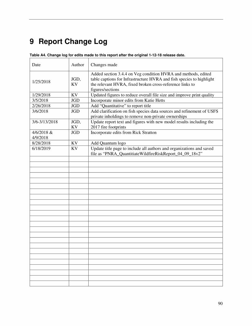
90
9 Report Change Log
Table A4. Change log for edits made to this report after the original 1-12-18 release date.
Date Author Changes made
1/25/2018 JGD,
KV
Added section 3.4.4 on Veg condition HVRA and methods, edited
table captions for Infrastructure HVRA and fish species to highlight
the relevant HVRA, fixed broken cross-reference links to
figures/sections
1/29/2018 KV Updated figures to reduce overall file size and improve print quality
3/5/2018 JGD Incorporate minor edits from Katie Hetts
2/26/2018 JGD Add “Quantitative” to report title
3/6/2018 JGD Add clarification on fish species data sources and refinement of USFS
private inholdings to remove non-private ownerships
3/6-3/13/2018 JGD,
KV
Update report text and figures with new model results including the
2017 fire footprints
4/6/2018 &
4/9/2018
JGD Incorporate edits from Rick Stratton
8/28/2018 KV Add Quantum logo
6/18/2019 KV Update title page to include all authors and organizations and saved
file as “PNRA_QuantitiateWildfireRiskReport_04_09_18v2”