Embed Size (px)
Citation preview

PacificJournal ofMathematics
LINES OF MINIMA ARE UNIFORMLY QUASIGEODESIC
YOUNG-EUN CHOI, KASRA RAFI AND CAROLINE SERIES
Volume 237 No. 1 September 2008

PACIFIC JOURNAL OF MATHEMATICSVol. 237, No. 1, 2008
LINES OF MINIMA ARE UNIFORMLY QUASIGEODESIC
YOUNG-EUN CHOI, KASRA RAFI AND CAROLINE SERIES
We continue the comparison between lines of minima and Teichmüller geo-desics begun in our previous work. For two measured laminations ν+ andν− that fill up a hyperbolizable surface S and for t ∈ (−∞, ∞), let Lt bethe unique hyperbolic surface that minimizes the length function et l(ν+) +
e−t l(ν−) on Teichmüller space. We prove that the path t 7→ Lt is a Teich-müller quasigeodesic.
1. Introduction
This paper continues the comparison between lines of minima and Teichmullergeodesics begun in [Choi et al. 2006]. Let S be a hyperbolizable surface of finitetype and T(S) be the Teichmuller space of S. Let ν+ and ν− be two measuredlaminations that fill up S. The associated line of minima is the path t 7→ Lt ∈ T(S),where Lt = Lt(ν
+, ν−) is the unique hyperbolic surface that minimizes the lengthfunction et l(ν+) + e−t l(ν−) on T(S); see [Kerckhoff 1992] and Section 2 be-low. Lines of minima have significance for hyperbolic 3-manifolds: infinitesimallybending Lt along the lamination ν+ results in a quasifuchsian group whose convexcore boundary has bending measures in the projective classes ν+ and ν− and inthe ratio e2t
: 1; see [Series 2005]. In this paper we prove:
Theorem A. The line of minima Lt for t ∈ R is a quasigeodesic with respect to theTeichmüller metric. In other words, there are universal constants c > 1 and C > 0,depending only on the topology of S, such that for any a, b ∈ R with a < b, we have
b − ac
− C ≤ dT(S)(La, Lb) ≤ c(b − a) + C,
where dT(S) is the Teichmüller distance.
An obvious way to approach this would be to compare the time-t surface Lt
with the corresponding surface Gt on the Teichmuller geodesic whose horizontaland vertical foliations at time t are respectively, etν+ and e−tν− [Gardiner andMasur 1991]. In [Choi et al. 2006], we did just this. We showed that if neithersurface Lt nor Gt contains short curves, that is, they are both contained in the thick
MSC2000: 30F60.Keywords: lines of minima, Teichmüller space, quasigeodesic.
21

22 YOUNG-EUN CHOI, KASRA RAFI AND CAROLINE SERIES
part of Teichmuller space, then the Teichmuller distance between them is boundedabove by a uniform constant that is independent of t . More generally, we showedthat the set of curves which are short on the two surfaces coincide. We also showed,however, that the ratio of lengths of the same short curve on the two surfaces maybe arbitrarily large so the path Lt may deviate arbitrarily far from Gt . It is thereforenot immediately obvious how to derive Theorem A from [Choi et al. 2006]. Toexplain our method, we first summarize the results of [Choi et al. 2006] in moredetail.
It turns out that on both Lt and Gt , a curve α is short if and only if at leastone of two quantities Dt(α) and Kt(α) is large. These quantities depend on thetopological relationship between α and the defining laminations ν+ and ν−. Theyrelate to the modulus of a maximal embedded annulus around α; the modulus of aflat annulus is approximately Dt(α) and the modulus of an expanding annulus isapproximately log Kt(α); see [Minsky 1992] and Sections 2 and 3 below. We saythat a curve is extremely short if it is less than some prescribed ε0 > 0 dependingonly on the topology of S; see Section 2. The essential results in [Choi et al. 2006]were the following estimates (see Section 2 for notation).
Theorem 1.1 [Choi et al. 2006, Theorems 5.10, 5.13, 7.13, 7.14]. Let α be a simpleclosed curve on S. If α is extremely short on Gt then
1lGt (α)
� max{Dt(α), log Kt(α)},
while if α is extremely short on Lt then
1lLt (α)
� max{
Dt(α),√
Kt(α)}.
Theorem 1.2 [Choi et al. 2006, Theorem 7.15]. The Teichmüller distance betweenLt and Gt is given by
dT(S)(Lt , Gt)+
�12 log max
α
{ lGt (α)
lLt (α)
},
where the maximum is taken over all simple closed curves α that are extremelyshort in Gt . In particular, the distance between the thick parts of Lt and Gt isbounded.
It follows from these results that, along intervals on which either there are noshort curves or Dt(α) dominates for all short curves α, the surfaces Lt and Gt
remain a bounded distance apart. However the path Lt may deviate arbitrarily farfrom Gt along time intervals on which Kt(α) is large and dominates Dt(α). Thesituation is complicated by the fact that as we move along Lt , the family of curves

LINES OF MINIMA ARE UNIFORMLY QUASIGEODESIC 23
which are short at a given point in time will vary with t , so the intervals alongwhich different curves α are short will overlap.
In addition to the above results from [Choi et al. 2006], there are two mainingredients in the proof of Theorem A. The first is a detailed comparison of therates of change of Kt(α) and Dt(α) with t . Some simple estimates are made inLemmas 3.1 and 3.2, with more elaborate consequences drawn in Lemma 5.1 andespecially Lemma 5.2. These results use Minsky’s product regions theorem (seeTheorem 2.4), which allows us to reduce calculations of distance in regions ofTeichmuller space in which a given family of curves is short, to straightforwardestimates in H2. To apply Minsky’s theorem, we need to compare not only lengthsbut also twists. We rely on the bounds on twists proved in [Choi et al. 2006] andreviewed in Theorems 2.8 and 2.9; these enter in a crucial way into the proof ofLemma 5.1.
The second main ingredient is control of distance along intervals along whichKt(α) is large. Consider the surface Sα obtained by cutting S along a short curve α
and replacing the two resulting boundary components by punctures. The followingrather surprising result, proved in Section 4, states that on intervals along whichKt(α) is large, we can estimate the Teichmuller distance by restricting to the Te-ichmuller space of the surface Sα. In other words, the contribution to Teichmullerdistance in Minsky’s formula 2.4 due to the short curve α itself may be neglected;see Theorem 4.1 for a precise statement.
Theorem B. If Kt(α) is sufficiently large for all t ∈ [a, b], the distance in T(Sα)
between the restrictions of Ga and Gb to Sα is equal to b − a, up to an additiveerror that is bounded by a constant depending only on the topology of S.
The proof of Theorem A requires estimating upper and lower bounds for
dT(S)(La, Lb)
over very large time intervals [a, b]. Given the first of the two ingredients above, theupper bound is relatively straightforward. The lower bound depends on Theorem B.The actual application involves a rather subtle inductive procedure based on Lemma5.2 which shows that at least one term in Minsky’s formula 2.4 always involves acontribution comparable to b − a.
The paper is organized as follows. Section 2 gives standard background and in-troduces the twist twσ (ξ, α) of a lamination ξ about a curve α with respect to a hy-perbolic metric σ . We give the main estimates about twists from [Choi et al. 2006].In Section 3, we recall from [Choi et al. 2006] the definitions of Dt(α) and Kt(α)
and derive some elementary results about their rates of change with t . In Section4 we prove Theorem B and in Section 5 we prove Theorem A.

24 YOUNG-EUN CHOI, KASRA RAFI AND CAROLINE SERIES
2. Background
Notation. Since we will be dealing mainly with coarse estimates, we want to avoidheavy notation and keep track of constants which are universal, in that they do notdepend on any specific metric or curve under discussion. For functions f , g wewrite f � g to mean that there are constants c ≥ 1, C ≥ 0, depending only on thetopology of S and the fixed constant ε0 (see below), such that
1c
g(x) − C ≤ f (x) ≤ cg(x) + C.
We usef ∗
� g and f+
� g
to mean that these inequalities hold with C = 0 and c = 1, respectively. Thesymbols ≺,
+
≺, ∗
≺, and so on, are defined similarly. In particular, we write X ≺ 1 toindicate X is bounded above by a positive constant depending only on the topologyof S and ε0.
Short curves. Let C(S) denote the set of isotopy classes of nontrivial, nonpe-ripheral simple closed curves on S. The length of the geodesic representative ofα ∈ C(S) with respect to a hyperbolic metric σ ∈ T(S) will be denoted lσ (α). Inour dealings with short curves we will have to make various assumptions to ensurethe validity of our estimates, which all require that the length lσ (α) of a “short”curve is less than various constants, in particular less than the Margulis constant.We suppose that ε0 > 0 is chosen once and for all to satisfy all needed assumptions,and say a simple closed curve α is extremely short in σ if lσ (α) < ε0.
Measured laminations and Teichmüller space. We denote the space of measuredlaminations on S by ML(S) and write lσ (ξ) for the hyperbolic length of a measuredlamination ξ ∈ ML(S). For ξ ∈ ML(S), we denote the underlying leaves by | ξ |.
Kerckhoff lines of minima. Suppose that ν+, ν−∈ ML(S) fill up S, meaning that
the sum of (geometric) intersections i(ν+, ξ) + i(ν−, ξ) > 0 for all ξ ∈ ML(S).Kerckhoff [1992] showed that the sum of length functions
σ 7→ lσ (ν+) + lσ (ν−)
has a unique global minimum on T(S). Moreover, as t varies in (−∞, ∞), theminimum Lt ∈ T(S) of l(ν+
t ) + l(ν−t ) for the measured laminations ν+
t = etν+
and ν−t = e−tν− varies continuously with t and traces out a path t 7→ Lt called the
line of minima L(ν+, ν−) of ν±.
Teichmüller geodesics. A pair of laminations ν+, ν−∈ML(S) which fill up S also
defines a Teichmuller geodesic G = G(ν+, ν−). The time-t surface Gt ∈ G is the

LINES OF MINIMA ARE UNIFORMLY QUASIGEODESIC 25
unique Riemann surface that supports a quadratic differential qt whose horizontaland vertical foliations are the measured foliations corresponding to ν+
t and ν−t
respectively; see [Gardiner and Masur 1991; Levitt 1983]. Flowing distance dalong G expands the vertical foliation by a factor ed and contracts the horizontalfoliation by e−d . By abuse of notation, we denote the hyperbolic metric on thesurface Gt also by Gt , and likewise denote the quadratic differential metric definedby qt also by qt .
Balance time. For a curve α ∈ C(S) that is not a component of either the verticalor the horizontal foliation, let tα denote the balance time of α at which
i(α, ν+
t ) = i(α, ν−
t ).
Along G, a curve is shortest near its balance time. More precisely, we have thefollowing proposition, which follows from [Rafi 2007, Theorem 3.1]:
Proposition 2.1. Choose ε > 0 so that ε < ε0 and suppose that lGtα(α) < ε. Let
Iα = Iα(ε) be the maximal connected interval containing tα such that lGt (α)< ε forall t ∈ Iα. Then there is a constant ε′ > 0 depending only on ε such that lGt (α) ≥ ε′
for all t /∈ Iα. (If lGtα(α) ≥ ε then set Iα = ∅.)
Curves which are components of the vertical foliation ( i(α, ν−) = 0, calledvertical) or the horizontal foliation ( i(α, ν+)=0, called horizontal) are exceptionalbut in general easier to handle. In such cases, tα is undefined. However, for reasonsof continuity, it is natural to adopt the convention that when α is vertical tα =
−∞ and when α is horizontal tα = ∞. Moreover, the arguments used to proveProposition 2.1 still hold; when α is vertical (respectively, horizontal), we define
Iα = (−∞, c) (respectively, Iα = (d, ∞))
to be the maximal interval where lGt (α) < ε.
Flat and expanding annuli. Let σ be a hyperbolic metric and let q be any qua-dratic differential metric in the same conformal class. Let A be an annulus in(S, q) with piecewise smooth boundary. The following notions are due to Minsky[1992]. We say A is regular if the boundary components ∂0, ∂1 are equidistant fromone another and the curvature along ∂0, ∂1 is either nonpositive at every point ornonnegative at every point (see [Minsky 1992] or [Choi et al. 2006] for details). Wefollow the sign convention that the curvature at a smooth point of ∂ A is positive ifthe acceleration vector points into A. Suppose A is a regular annulus such that thetotal curvature of ∂0 satisfies κ(∂0) ≤ 0. Then, it follows from the Gauss–Bonnettheorem that κ(∂1)≥0. We say A is flat if κ(∂0)=κ(∂1)=0 and say A is expandingif κ(∂0) < 0, and call ∂0 the inner boundary and ∂1 the outer boundary.

26 YOUNG-EUN CHOI, KASRA RAFI AND CAROLINE SERIES
A regular annulus is primitive if it contains no singularities of q in its interior. Itfollows that a flat annulus is primitive and is isometric to a cylinder obtained from aEuclidean rectangle by identifying one pair of parallel sides. An expanding annulusthat is primitive is coarsely isometric to an annulus bounded by two concentriccircles in the plane.
The length of a curve α which is short in (S, σ ) can be estimated by the modulusof a primitive annulus around it:
Theorem 2.2 [Minsky 1992, Theorem 4.5; Choi et al. 2006, Theorem 5.3]. Sup-pose α ∈ C(S) is extremely short in (S, σ ). Then for any quadratic differentialmetric q in the same conformal class as σ , there is an annulus A that is primitivewith respect to q whose core is homotopic to α such that
1lσ (α)
� Mod(A).
The modulus of a primitive annulus is estimated as follows:
Theorem 2.3 [Minsky 1992, Theorem 4.5; Rafi 2005, Lemma 3.6]. Let A ⊂ S bea primitive annulus. Let d be the q-distance between the boundary components ∂0,∂1. If A is expanding let ∂0 be the inner boundary. Then either
(i) A is flat and Mod A = d/ lq(∂0) = d/ lq(∂1) or
(ii) A is expanding and Mod A � log(d/ lq(∂0)).
Minsky’s product regions theorem. Our main tool for estimating Teichmuller dis-tance is Minsky’s product regions theorem, which reduces the estimation of thedistance between two surfaces on which a given set 0 of curves is short to a cal-culation in the hyperbolic plane H2. To give a precise statement, we introduce thefollowing notation. Choose a pants curves system on S that contains 0, and for acurve α in the pants system let sα(σ ) be the Fenchel–Nielsen twist coordinate of α.(Here sα(σ ) = sα(σ )/ lσ (α), where sα(σ ) is the actual hyperbolic distance twistedround α; see Minsky [1996] for details.) Let Tthin(0, ε0) be the subset of T(S)
on which all the curves in 0 have length less than ε0 and let S0 be the analyticallyfinite surface obtained from S by pinching all the curves in 0. By forgetting theFenchel–Nielsen length and twist coordinates associated to the curves in 0 butretaining all remaining Fenchel–Nielsen coordinates, we obtain a projection
50 : T(S) → T(S0).
For each α ∈ 0, let Hα denote a copy of the upper-half plane and let d Hαdenote
half the usual hyperbolic metric on Hα (see [Minsky 1996, Lemma 2.2] for thefactor). Define 5α : T(S) → Hα by 5α(σ ) = sα(σ ) + i/ lσ (α) ∈ Hα. Then theproduct regions theorem states:
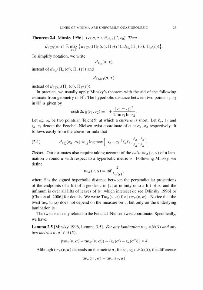
LINES OF MINIMA ARE UNIFORMLY QUASIGEODESIC 27
Theorem 2.4 [Minsky 1996]. Let σ, τ ∈ Tthin(0, ε0). Then
dT(S)(σ, τ )+
� maxα∈0
{dT(S0)(50(σ ), 50(τ )), d Hα
(5α(σ ), 5α(τ ))}.
To simplify notation, we writed Hα
(σ, τ )
instead of d Hα(5α(σ ), 5α(τ )) and
dT(S0)(σ, τ )
instead of dT(S0)(50(σ ), 50(τ )).In practice, we usually apply Minsky’s theorem with the aid of the following
estimate from geometry in H2. The hyperbolic distance between two points z1, z2
in H2 is given by
cosh 2d H(z1, z2) = 1 +| z1 − z2 |
2
2 Im z1Im z2.
Let σa , σb be two points in Teich(S) at which a curve α is short. Let `a , `b andsa , sb denote the Fenchel–Nielsen twist coordinate of α at σa , σb respectively. Itfollows easily from the above formula that
(2-1) d H2α(σa, σb)
+
�12 log max
{| sa − sb|
2`a`b,`a
`b,`b
`a
}.
Twists. Our estimates also require taking account of the twist twσ (ν, α) of a lam-ination ν round α with respect to a hyperbolic metric σ . Following Minsky, wedefine
twσ (ν, α) = infs
lσ (α),
where s is the signed hyperbolic distance between the perpendicular projectionsof the endpoints of a lift of a geodesic in |ν| at infinity onto a lift of α, and theinfimum is over all lifts of leaves of |ν| which intersect α; see [Minsky 1996] or[Choi et al. 2006] for details. We write Twσ (ν, α) for | twσ (ν, α)|. Notice that thetwist twσ (ν, α) does not depend on the measure on ν, but only on the underlyinglamination |ν|.
The twist is closely related to the Fenchel–Nielsen twist coordinate. Specifically,we have:
Lemma 2.5 [Minsky 1996, Lemma 3.5]. For any lamination ν ∈ ML(S) and anytwo metrics σ, σ ′
∈ T(S),∣∣(twσ (ν, α)− twσ ′(ν, α))− (sα(σ ) − sα(σ ′))∣∣ ≤ 4.
Although twσ (ν, α) depends on the metric σ , for ν1, ν2 ∈ ML(S), the difference
twσ (ν1, α)− twσ (ν2, α)

28 YOUNG-EUN CHOI, KASRA RAFI AND CAROLINE SERIES
is independent of σ up to a universal additive constant; see [Minsky 1996; Choiet al. 2006, Section 4]. This motivates the following definition:
Definition 2.6. For α ∈ C(S) and ν1, ν2 ∈ ML(S), the relative twist of ν1 and ν2
round α is
dα(ν1, ν2) = infσ
| twσ (ν1, α)− twσ (ν2, α)|,
where the infimum is taken over all hyperbolic metrics σ ∈ T(S).
(The relative twist dα(ν1, ν2) agrees up to an additive constant with the definitionof subsurface distance between the projections of |ν1| and |ν2| to the annular coverof S with core α, as defined in [Masur and Minsky 2000, Section 2.4] and usedthroughout [Rafi 2005; 2007].)
Rafi [2007] (see also [Choi et al. 2006, Section 5.4]) introduced a similar notionof the twist twq(ν, α) with respect to a quadratic differential metric q compatiblewith σ and proved the following result, which enters into the proof of Theorem4.1:
Proposition 2.7 Rafi 2007, Theorem 4.3; Choi et al. 2006, Proposition 5.7. Sup-pose that σ ∈ T(S) is a hyperbolic metric and q is a compatible quadratic differ-ential metric. For any geodesic lamination ξ intersecting α, we have
| twσ (ξ, α)− twq(ξ, α)| ≺1
lσ (α).
We shall also need the following important estimates of the twist which comple-ment Theorem 1.1. If α is vertical or horizontal, tα is defined using the conventiondiscussed following Proposition 2.1.
Theorem 2.8 [Choi et al. 2006, Theorems 5.11, 5.13]. Let α be a simple closedcurve on S. If α is extremely short on Gt then
Tw Gt (ν+, α) ≺
1lGt (α)
if t > tα,
Tw Gt (ν−, α) ≺
1lGt (α)
if t < tα.
Theorem 2.9 [Choi et al. 2006, Theorems 6.2, 6.9]. Let α be a simple closed curveon S. If α is extremely short on Lt then
TwLt (ν+, α) ≺
1lLt (α)
if t > tα,
TwLt (ν−, α) ≺
1lLt (α)
if t < tα.

LINES OF MINIMA ARE UNIFORMLY QUASIGEODESIC 29
3. The length estimates
In this section we discuss the quantities Dt(α) and Kt(α) that appear in the lengthestimates in Theorem 1.1.
Let qt be the unit-area quadratic differential metric on Gt whose vertical andhorizontal foliations are etν+ and e−tν−, respectively. In light of Theorems 2.2and 2.3, to estimate the length of a curve α which is extremely short in Gt , it issufficient to estimate the modulus of a maximal flat or expanding annulus around α
in qt . The union of all qt -geodesic representatives of α foliate a Euclidean cylinderFt(α), which is the maximal flat annulus whose core is homotopic to α. (Thecylinder is degenerate if the representative of α is unique.) On either side of Ft(α)
is attached a maximal expanding annulus. Let Et(α) be the one of larger modulus.Up to coarse equivalence, Dt(α) will be the modulus of Ft(α) while log Kt(α) willbe the modulus of Et(α).
The precise definition of Dt(α) is as follows. If α is not a component of |ν±|,
we define
(3-1) Dt(α) = e−2 |t−tα | dα(ν+, ν−),
where dα(ν+, ν−) is the relative twisting of ν+ and ν− about α as defined above.If α is vertical, define
Dt(α) = e−2t Mod F0(α)
and if α is horizontal, define
Dt(α) = e2t Mod F0(α),
where F0(α) is the annulus at time t = 0.The precise definition of Kt(α) is
(3-2) Kt(α) =dqt
lqt (∂0),
where ∂0 is the inner boundary of Et(α) and dqt is the qt -distance between theinner and outer boundaries of Et(α).
The connection with the definition of Kt(α) in [Choi et al. 2006] and the reasonswhy Dt(α) and Kt(α) are coarsely the moduli of Ft(α) and Et(α) respectively areexplained at the end of this section. The estimate for 1/ lGt (α) in Theorem 1.1follows easily from the above definitions and Minsky’s estimates. The estimate for1/ lLt (α) in the same theorem required a lengthy separate analysis. The only fea-tures of these definitions which will concern us here are the estimates in Theorem1.1 and the relative rates of change of Dt(α) and Kt(α) with time.
30 YOUNG-EUN CHOI, KASRA RAFI AND CAROLINE SERIES
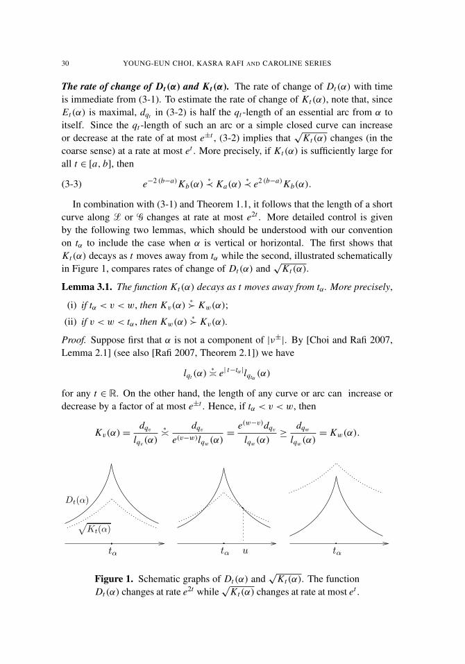
The rate of change of Dt(α) and K t(α). The rate of change of Dt(α) with timeis immediate from (3-1). To estimate the rate of change of Kt(α), note that, sinceEt(α) is maximal, dqt in (3-2) is half the qt -length of an essential arc from α toitself. Since the qt -length of such an arc or a simple closed curve can increaseor decrease at the rate of at most e±t , (3-2) implies that
√Kt(α) changes (in the
coarse sense) at a rate at most et . More precisely, if Kt(α) is sufficiently large forall t ∈ [a, b], then
(3-3) e−2 (b−a)Kb(α)∗
≺ Ka(α)∗
≺ e2 (b−a)Kb(α).
In combination with (3-1) and Theorem 1.1, it follows that the length of a shortcurve along L or G changes at rate at most e2t . More detailed control is givenby the following two lemmas, which should be understood with our conventionon tα to include the case when α is vertical or horizontal. The first shows thatKt(α) decays as t moves away from tα while the second, illustrated schematicallyin Figure 1, compares rates of change of Dt(α) and
√Kt(α).
Lemma 3.1. The function Kt(α) decays as t moves away from tα. More precisely,
(i) if tα < v < w, then Kv(α)∗
� Kw(α);
(ii) if v < w < tα, then Kw(α)∗
� Kv(α).
Proof. Suppose first that α is not a component of |ν±|. By [Choi and Rafi 2007,
Lemma 2.1] (see also [Rafi 2007, Theorem 2.1]) we have
lqt (α)∗
� e| t−tα |lqtα(α)
for any t ∈ R. On the other hand, the length of any curve or arc can increase ordecrease by a factor of at most e±t . Hence, if tα < v < w, then
Kv(α) =dqv
lqv(α)
∗
�dqv
e(v−w)lqw(α)
=e(w−v)dqv
lqw(α)
≥dqw
lqw(α)
= Kw(α).
√
Kt(α)
tαtα
Dt(α)
utα
Figure 1. Schematic graphs of Dt(α) and√
Kt(α). The functionDt(α) changes at rate e2t while
√Kt(α) changes at rate at most et .

LINES OF MINIMA ARE UNIFORMLY QUASIGEODESIC 31
A similar argument can be applied in the case when v < w < tα.If α is vertical, then
lqt (α)∗
� et lq0(α),
while if it is horizontallqt (α)
∗
� e−t lq0(α).
The result then follows in the same way. �
Lemma 3.2. Let Iα be as in Proposition 2.1 and let [a, b] ⊂ Iα. Suppose thatDu(α) =
√Ku(α) for some u ∈ [a, b] .
(i) If tα < u, then√
Kt(α)∗
� Dt(α) for all t ∈ [u, b].
(ii) If u < tα, then√
Kt(α)∗
� Dt(α) for all t ∈ [a, u].
Proof. We refer to Figure 1 for a schematic picture of the two graphs. The proof isbased on the fact that
√Kt(α) decays at a slower rate than Dt(α) as t moves away
from tα. If tα < u, then for any t > u we have
Kt(α) =dqt
lqt (α)
∗
�e−(t−u)dqu
e(t−u)lqu (α)= e−2(t−u)Ku(α).
Therefore, √Kt(α)
∗
� e−(t−u)Du(α) = e(t−u)Dt(α) ≥ Dt(α).
A similar argument can be applied in the case when u < tα. �
Alternative definitions of Dt(α) and K t(α). The remarks which follow are notessential for the proof of Theorem A but may be helpful in clarifying backgroundfrom [Choi et al. 2006].
The claim that Dt(α) is coarsely equal to the modulus of Ft(α) is justified by[Choi et al. 2006, Proposition 5.8 (Section 5.6 for the exceptional case)] whichstates that ModFt(α) � Dt(α). The proof is an exercise in Euclidean geometry,combined with Rafi’s comparison Proposition 2.7 between the twist in the quadraticand hyperbolic metrics. For example, at the balance time tα, the horizontal andvertical leaves both make an angle π/4 with the qtα -geodesic representatives of α.Let η be an arc joining the two boundary components of Ftα that is orthogonal toall the qtα -geodesic representatives of α. In this case, a leaf of ν+
tα or ν−tα intersects η
approximately (up to an error of 1) lqtα(η)/ lqtα
(α) times, so the modulus of Ftα (α)
is approximated byTwFtα
(ν+, α) = TwFtα(ν−, α),
where twFtα(and TwFtα
) means the twist in the q-metric restricted to Ftα . Theresult would follow by noting that twFtα
(ν+, α) and twFtα(ν−, α) have opposite
signs, except that dα involves hyperbolic twists on S rather than q-twists in Ftα .This is resolved using Proposition 2.7; see [Choi et al. 2006] for further details.
32 YOUNG-EUN CHOI, KASRA RAFI AND CAROLINE SERIES
That log Kt(α) is coarsely the modulus of Et(α) follows from Theorem 2.3. Theabove is not the definition of Kt(α) given in [Choi et al. 2006], but it is coarselyequivalent. Specifically, let Y1, Y2 be the (possibly coincident) thick componentsadjacent to α in the thick-thin decomposition of the hyperbolic metric Gt . Set
Jt(α) =1
lqt (α)max{λY1, λY2}
where λYi is the length of the shortest nontrivial nonperipheral simple closed curveon Yi with respect to the metric qt . (If either Yi is a pair of pants there is a slightlydifferent definition; see [Choi et al. 2006].) In [Choi et al. 2006], we took the aboveexpression for Jt(α) as the definition of Kt(α). [Choi et al. 2006, Proposition 5.9]shows that if Jt(α) is sufficiently large, then Jt(α)
∗
� Kt(α) with Kt(α) defined asin (3-2) above.
4. Expanding annuli that persist
It follows from Theorems 1.1 and 1.2 that if Dt(α) ≥√
Kt(α) for every α that isshort in Gt , then the distance dT(S)(Gt , Lt) is uniformly bounded. Moreover, if Gt isin the thick part of Teichmuller space, then Lt is too, so that on such intervals Lt isquasigeodesic. Thus our attention is focused on time intervals along which Kt(α)
is large. This is handled with the following more precise version of Theorem B.
Theorem 4.1. Choose M > 0 to be a constant such that if Kt(α) > M then α
is extremely short in Gt . (This is possible due to Theorem 1.1.) Suppose thatKt(α) > M for all t ∈ [a, b]. Then
dT(Sα)(Ga, Gb)+
� b − a.
Corollary 4.2. Let 0 be a family of disjoint curves on S such that Kt(α) > M forall t ∈ [a, b] and for every α ∈ 0. Then
dT(S0)(Ga, Gb)+
� b − a.
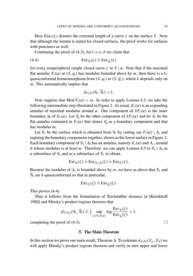
Proof. We prove the statement of the theorem; the corollary is immediate. Theidea is that for each t ∈ [a, b], we cut the maximal flat annulus around α in (S, qt)
out of S and reglue the two boundary components, obtaining a new surface Gt ;see Figure 2. The surfaces Gt will also move along a Teichmuller geodesic. Inparticular
dT(S)(Ga, Gb) = b − a.
On the other hand, Gt contains the same expanding cylinders round α as Gt so thatKGt
(α) = Kt(α). Consideration of the rate of change of Kt with time shows thatthe contribution to the change in Teichmuller distance between Ga and Gb from the

LINES OF MINIMA ARE UNIFORMLY QUASIGEODESIC 33
∂0 ∂′
0
At
Zt
GtGt
Figure 2. Cut out flat annulus and reglue.
expanding cylinders is of the order of log(b−a), so the actual distance b−a mustbe realized due to changes in T(Sα).
In more detail, this works as follows. Let F = Fa(α) be the maximal flat annulusaround α in (S, qa). The arcs in F that are perpendicular to ∂ F define an isometryf from one component of ∂ F to the other. Let Ga be the surface obtained byremoving F and gluing the components of ∂ F together via f (also making sure topreserve the marking); see the upper two surfaces in Figure 2. Let α be the gluingcurve in Ga . Since the vertical and horizontal foliations of qa match along α, thesurface Ga is naturally equipped with vertical and horizontal foliations ν±
a andquadratic differential qa , which is assumed to be scaled to have area one. Let {Gt }
be the Teichmuller geodesic corresponding to qa and let q t be the correspondingfamily of quadratic differentials. Then
dT(S)(Ga, Gb) = b − a.
Observe that the surface Gt is obtained from Gt by cutting out the maximal flatannulus Ft = Ft(α). Thus, for each t , we have a natural map
ϕt : (S, qt) \ Ft → (S, q t) \ α
which fixes points but scales the metric. Hence, Kq t (α) = Kt(α) > M on [a, b]
and therefore α is also extremely short in Gt on [a, b]. Applying Theorem 2.4, weget
(4-1) b − a = dT(S)(Ga, Gb)+
� max{dT(Sα)(Ga, Gb), d H2
α(Ga, Gb)
}.
To prove the theorem, it will suffice to establish the following two bounds:
(4-2) d H2α(Ga, Gb) ≺ log(b − a),
and
(4-3) dT(Sα)(Ga, Ga) ≺ 1, dT(Sα)(Gb, Gb) ≺ 1.
34 YOUNG-EUN CHOI, KASRA RAFI AND CAROLINE SERIES
The theorem would then follow from (4-1), (4-2), (4-3) and the triangle inequality.
Proof of (4-2). We use the estimate of distance in H2α from (2-1) in Section 2. Let
σt = Gt , let `t = lσt (α), and let st be the Fenchel–Nielsen twist coordinate of α atσt . By (2-1) we have
d H2α(σa, σb)
+
�12 log max
{| sa − sb|
2`a`b,`a
`b,`b
`a
}.
We shall show that the contribution | sa − sb|2`a`b coming from the twist can be
neglected. By Lemma 2.5, we have
| sa − sb|+
� | twσa (ξ, α)− twσb(ξ, α)|
for any lamination ξ . By Proposition 2.7 with ξ = ν+ (or ξ = ν−), we have∣∣Twσa (ν+, α)− Twqa (ν
+, α)∣∣ ≺
1`a
,∣∣Twσb(ν
+, α)− Twqb(ν+, α)
∣∣ ≺1`b
.
In general, if a curve α is short on a surface σ then, by considering the restrictionto F , we can view twq(ν, α) as split into contributions coming from the flat and theexpanding annuli around α. It follows from the Gauss–Bonnet theorem that in anexpanding annulus, two geodesics intersect at most once. Hence the contributionto twq(ν, α) is essentially contained in F(α); for details see [Rafi 2007] and theproof of [Choi et al. 2006, Lemma 5.6].
In the present case, there is no flat annulus in q t corresponding to α. Hence thetwistings Twqa (ν
+, α) and Twqb(ν+, α) are bounded; in fact, they are at most two.
Therefore, | sa − sb|2`a`b ≺ 1 and we get
d H2α(σa, σb)
+
�12 log max
{`a
`b,`b
`a
}.
Since Kqa (α) = Ka(α) and Kqb(α) = Kb(α), it follows from (3-3) that
`a
`b�
log Kb(α)
log Ka(α)≺
2(b − a) + log Ka(α)
log Ka(α)≤
2(b − a)
log M+ 1.
Similarly for `b/`a , we have the identical bound. Thus (4-2) is proved.
Proof of (4-3). This is a consequence of the following lemma due to Minsky.
Lemma 4.3 [Minsky 1992, Lemma 8.4]. Let X be a closed Riemann surface andY ⊂ X an incompressible subsurface. There exists a constant m depending on thetopology of X only, such that if each component of ∂Y bounds an annulus in Y ofmodulus at least m, then for any nonperipheral simple closed curve ζ ⊂ Y ,
ExtY(ζ )∗
� ExtX(ζ ).
LINES OF MINIMA ARE UNIFORMLY QUASIGEODESIC 35
Here ExtY(ζ ) denotes the extremal length of a curve ζ on the surface Y . Notethat although the lemma is stated for closed surfaces, the proof works for surfaceswith punctures as well.
Continuing the proof of (4-3), for t = a, b we claim that
(4-4) Ext Gt(ζ )∗
� Ext Gt(ζ )
for every nonperipheral simple closed curve ζ in S \ α. Note that if the maximalflat annulus Ft(α) at (S, qt) has modulus bounded above by m, then there is a k-quasiconformal homeomorphism from (S, qt) to (S, q t), where k depends only onm. This automatically implies that
dT(S)(Gt , Gt) ≺ 1.
Now suppose that Mod Ft(α) > m. In order to apply Lemma 4.3, we take thefollowing intermediate step illustrated in Figure 2. As usual, Et(α) is an expandingannulus of maximal modulus around α. One component of ∂ Ft(α) is the innerboundary ∂0 of Et(α). Let ∂ ′
0 be the other component of ∂ Ft(α) and let At be theflat annulus contained in Ft(α) that shares ∂ ′
0 as a boundary component and thathas modulus m.
Let Zt be the surface which is obtained from Gt by cutting out Ft(α) \ At andregluing the boundary components together, shown as the lower surface in Figure 2.Each boundary component of Zt \∂0 has an annulus, namely Et(α) and At , aroundit whose modulus is at least m. Therefore, we can apply Lemma 4.3 to Zt \ ∂0 asa subsurface of Gt and as a subsurface of Zt to obtain
Ext Gt(ζ )∗
� Ext Zt\∂0(ζ )∗
� Ext Zt(ζ ).
Because the modulus of At is bounded above by m, we have as above that Zt andGt are k-quasiconformal so that in particular,
Ext Zt(ζ )∗
� Ext Gt(ζ ).
This proves (4-4).Thus it follows from the formulation of Teichmuller distance in [Kerckhoff
1980] and Minsky’s product regions theorem that
dT(Sα)(Gt , Gt)+
�12 sup
ζ∈C(S\α)
logExt Gt(ζ )
Ext Gt(ζ )
≺ 1,
completing the proof of (4-3). �
5. The Main Theorem
In this section we prove our main result, Theorem A. To estimate dT(S)(La, Lb) wewill apply Minsky’s product regions theorem and verify in turn upper and lower
36 YOUNG-EUN CHOI, KASRA RAFI AND CAROLINE SERIES
bounds on the distance. We start with a lemma which will be used to estimated H2
α(Lv, Lw), where α is a curve which is short along an interval [v, w].
Recall from Proposition 2.1 that Iα = Iα(ε) is the maximal open interval aroundtα such that lGt (α) < ε for all t ∈ Iα. It follows from Theorem 1.1 that if a curveis sufficiently short in Gt , then it is, in the coarse sense, at least as short in Lt . Inparticular, we may choose ε =ε1 in Proposition 2.1 small enough that if lGt (α)<ε1,then lLt (α) < ε0.
Lemma 5.1. Let [v, w] ⊂ Iα(ε1).
(i) If Dt(α) ≥√
Kt(α) for all t ∈ [v, w], then
d H2α(Lv, Lw)
+
� w − v.
(ii) If√
Kt(α) ≥ Dt(α) for all t ∈ [v, w], then
d H2α(Lv, Lw)
+
≺w − v
2.
Proof. The proof rests on the formula (2-1) from Section 2 and a careful comparisonof rates of change of lengths and twists. Let `t = lLt (α), and let st be the Fenchel–Nielsen twist of α at Lt . As in (2-1) we have
(5-1) d H2α(Lv, Lw)
+
�12 log max
{| sv − sw|
2`v`w,`v
`w
,`w
`v
}.
By Lemma 2.5, we have
| sv − sw|+
�∣∣ twLv
(ν±, α)− twLw(ν±, α)
∣∣.First suppose tα ≤ v < w. Then by Theorem 2.9,
| sv − sw|2`v`w
∗
≺
( 1`v
+1`w
)2`v`w
∗
� max{ `v
`w
,`w
`v
}.
Therefore,
d H2α(Lv, Lw)
+
�12 log max
{ `v
`w
,`w
`v
}.
If Dt(α) ≥√
Kt(α) for all t ∈ [v, w], so that 1/ lLt (α)∗
� Dt(α) on [v, w], then
max{ `v
`w
,`w
`v
}∗
� e2(w−v).
If√
Kt(α) ≥ Dt(α) for all t ∈ [v, w], so that 1/ lLt (α)∗
�√
Kt(α) on [v, w], thenby (3-3) and Lemma 3.1, we get√
Kw(α)∗
≺
√Kv(α)
∗
≺ ew−v√
Kw(α),

LINES OF MINIMA ARE UNIFORMLY QUASIGEODESIC 37
from which it follows that
max{ `v
`w
,`w
`v
}∗
≺ ew−v
and the lemma is proved in this case. The case where v < w ≤ tα can be handledsimilarly.
Now, suppose v < tα < w and for convenience, translate so that tα = 0. If√
Kt(α) ≥ Dt(α) for all t ∈ [v, w], the result follows from the triangle inequality
d H2α(Lv, Lw) ≤ d H2
α(Lv, L0) + d H2
α(L0, Lw)
and is already proved above.The interesting case is that in which Dt(α)≥
√Kt(α) for all t ∈ [v, w], in which
case lLt (α) decreases on [v, 0] but then increases again on [0, w]. This means that
max{ `v
`w
,`w
`v
}∗
� e2 |v+w|
and consequently the term
12 log max
{ `v
`w
,`w
`v
}does not reflect the total distance w − v. Instead, we have to look more carefullyat the term |sv − sw|
2`v`w.We have
| sv − sw| `v+
� | twLv(ν−, α)− twLw
(ν−, α)| `v+
� TwLw(ν−, α) `v
where the second equality follows from Theorem 2.9. Similarly,
| sv − sw| `w+
� | twLv(ν+, α)− twLw
(ν+, α)| `w+
� TwLv(ν+, α) `w.
On the other hand, writing dα = dα(ν+, ν−) for the relative twist as defined inSection 2, we get
dα`v+
� | twLv(ν−, α)− twLv
(ν+, α)| `v+
� TwLv(ν+, α)`v,
dα`w+
� | twLw(ν−, α)− twLw
(ν+, α)| `w+
� TwLw(ν−, α)`w,
where we again made two applications of Theorem 2.9.Also note that by definition, D0(α) = dα so by Theorem 1.1 we have 1/`0
∗
� dα.Thus
| sv − sw|2`v`w
∗
� d2α`v`w
∗
�`v
`0
`w
`0= e2(w−v).
It follows by (5-1) thatd H2
α(Lv, Lw)
+
� w − v. �

38 YOUNG-EUN CHOI, KASRA RAFI AND CAROLINE SERIES
Before proving our main theorem, we also establish the following rather tech-nical lemma, which quantifies more precisely the schematic graphs in Figure 1.Lemma 5.2. Let M be chosen as in Theorem 4.1. Then there exists ε > 0, depend-ing only on the topology of S, such that for any a, b with [a, b] ⊂ Iα(ε), one of thefollowing alternatives holds:
(i) Kt(α) > M on [a, b];
(ii) item (i) fails, Dt(α) ≥√
Kt(α) on a subinterval of the form [a, u] and√Kb(α)
∗
≺ eu−a;
(iii) item (i) fails, Dt(α) ≥√
Kt(α) on a subinterval of the form [u, b] and√Ka(α)
∗
≺ eb−u .
Proof. By Theorem 1.1, we can choose ε > 0 small enough that if t ∈ Iα(ε) andif
√Kt(α) ≥ Dt(α) then Kt(α) > M . Thus if (i) fails, we must have Dw(α) >
√Kw(α) for some w ∈ (a, b).Suppose first that Dt(α) >
√Kt(α) on [a, b], and that (i) fails, so that there is
some c ∈ [a, b] where Kc(α) ≤ M . To check (ii) holds, we only have to verify itsfinal statement. Since M is fixed, it follows from (3-3) that√
Kb(α)∗
≺ eb−c√
Kc(α)∗
≺ eb−a.
(By the same argument, (iii) also holds in this case.)Now suppose that Du(α) =
√Ku(α) for some u ∈ (a, b). We claim that if
tα /∈ [a, b] then (i) holds. Suppose for definiteness that tα < a. By Lemma 3.1 wehave Kt(α)
∗
� Ku(α) on [a, u], and by Lemma 3.2 we have√
Kt(α)∗
� Dt(α) on[u, b]. Hence 1/ lLt (α)�
√Kt(α) on [u, b]. Therefore, reducing ε >0 if necessary,
we can again ensure Kt(α) > M on [a, b] and (i) holds as claimed.Suppose now that Du(α) =
√Ku(α) for some u ∈ [a, b] and that tα ∈ [a, b],
say for definiteness that tα < u. If there is another point u′∈ [a, tα] such that
Du′(α) =√
Ku′(α), then again with a suitable adjustment of ε we have Kt(α) > Mon [a, b] (see Figure 1) and we are in case (i). If there is no such point u′, thenDt(α) ≥
√Kt(α) on [a, u]. Assuming that in addition (i) fails, there is a point
c ∈[a, b] where Kc(α)≤ M . By Lemma 3.2 we have 1/ lLt (α)∗
�√
Kt(α) on [u, b].Assuming ε is sufficiently small, we deduce that c ∈ [a, u]. Then by Lemma 3.1we have√
Kc(α)∗
� e−| tα−c |√
Ktα (α)∗
� e−| tα−c |√
Kb(α) ≥ e−(u−a)√
Kb(α)
and we are in case (ii). The case where tα > u is handled similarly and results in(iii). �
LINES OF MINIMA ARE UNIFORMLY QUASIGEODESIC 39
Proof of Theorem A. As noted in Section 1, we prove the theorem by obtainingseparate upper and lower bounds for dT(S)(La, Lb). The upper bound is rela-tively straightforward but the lower bound requires an inductive procedure basedon Lemma 5.2.
In order to compare two surfaces La , Lb at the ends of a long interval [a, b]⊂ R,it is convenient to consider separately the curves which are short at a but not at b,those which are short at b but not at a, and those which are short at both. More pre-cisely, choose ε to satisfy Lemma 5.2 and then choose ε′
≤ ε as in Proposition 2.1so that if lGt (α) < ε′ then t ∈ Iα(ε). In particular, if lGa (α) < ε′ and lGb(α) < ε′,then since Iα(ε) is connected, [a, b] ⊂ Iα(ε). Now define subsets 0a , 0b and 0 ofthe curves of length less than ε′ in either Ga or Gb as follows:
0a = {α ∈ C(S) : lGa (α) < ε′, lGb(α) ≥ ε′},
0b = {α ∈ C(S) : lGb(α) < ε′, lGa (α) ≥ ε′},
0 = {α ∈ C(S) : lGt (α) < ε′, for t = a, b}.
We begin by establishing some preliminary estimates on distances in the Te-ichmuller spaces of the subsurfaces obtained by cutting along these curves. ByMinsky’s product regions theorem,
dT(S0)(La, Ga)+
� maxα∈0a
{dT(S0∪0a )(La, Ga), d H2
α(La, Ga)
},
dT(S0)(Lb, Gb)+
� maxα∈0b
{dT(S0∪0b )(Lb, Gb), d H2
α(Lb, Gb)
}.
Now on the one hand, by Theorem 1.2, the thick parts of Ga and La are boundeddistance from one another, as are the those of Gb and Lb. Therefore,
dT(S0∪0a )(La, Ga) ≺ 1 and dT(S0∪0b )(Lb, Gb) ≺ 1.
On the other hand, because the twisting is bounded as in Theorems 2.8 and 2.9,we have
d H2α(La, Ga)
+
≺12 log
lGa (α)
lLa (α)< 1
2 log1
lLa (α)for α ∈ 0a ,
d H2α(Lb, Gb)
+
≺12 log
lGb(α)
lLb(α)< 1
2 log1
lLb(α)for α ∈ 0b.
Thus it follows that
(5-2)
dT(S0)(La, Ga)+
≺12 max
α∈0a
{log
1lLa (α)
},
dT(S0)(Lb, Gb)+
≺12 max
α∈0b
{log
1lLb(α)
}.
40 YOUNG-EUN CHOI, KASRA RAFI AND CAROLINE SERIES
We now turn to bounding the distance dT(S)(La, Lb). By Minsky’s productregions theorem,
(5-3) dT(S)(La, Lb)+
� maxα∈0
{dT(S0)(La, Lb), d H2
α(La, Lb)
}.
Upper bound. We prove the upper bound dT(S)(La, Lb)+
≺ 3(b − a) by boundingthe terms on the right hand side of (5-3).
By Lemma 5.1 we have d H2α(La, Lb)
+
≺ b − a for each α ∈ 0. We provide anupper bound for dT(S0)(La, Lb) using the triangle inequality
(5-4) dT(S0)(La, Lb) ≤ dT(S0)(La, Ga) + dT(S0)(Ga, Gb) + dT(S0)(Lb, Gb).
To bound the first and last terms of the right hand side, we will use (5-2) and thefact that the length lLt (α) of a curve increases at rate at most e2t . More precisely,notice that if α ∈ 0a then Iα ∩ [a, b] = [a, c) for some c ≤ b. By definition ofIα, we have lGc(α) = ε. Then it follows from Theorem 1.1 that lLc(α) is boundedbelow by a uniform constant that depends only on ε. Therefore, by the observationfollowing (3-3), we have
log1
lLa (α)
+
≺ loglLc(α)
lLa (α)
+
≺ 2(b − a).
Similarly, if α ∈ 0b, then
log1
lLb(α)
+
≺ 2(b − a).
Therefore, from (5-2) it follows that
dT(S0)(La, Ga)+
≺ b − a and dT(S0)(Lb, Gb)+
≺ b − a.
The second term in (5-4) is bounded by Minsky’s product regions theorem:
dT(S0)(Ga, Gb)+
≺ dT(S)(Ga, Gb) = b − a.
This finishes the proof of the upper bound.
Lower bound. We prove the lower bound dT(S)(La, Lb)+
� (b − a)/4 by showingthat at least one of the terms in the right hand side of (5-3) is bounded below by(b − a)/4.
We begin by reducing the problem to a consideration of the curves in 0 only. Itfollows from a theorem of Wolpert [1979] that for every γ ∈ C(S),
dT(S)(La, Lb) ≥12
∣∣∣ loglLb(γ )
lLa (γ )
∣∣∣.

LINES OF MINIMA ARE UNIFORMLY QUASIGEODESIC 41
It follows as before from Theorem 1.1 that if lGt (α) ≥ ε′, then the length lLt (α) isuniformly bounded below. Therefore, we have∣∣∣ log
lLb(α)
lLa (α)
∣∣∣ +
� log1
lLa (α)for α ∈ 0a ,∣∣∣ log
lLa (α)
lLb(α)
∣∣∣ +
� log1
lLb(α)for α ∈ 0b.
It follows from the triangle inequality that if either
maxα∈0a
{log
1lLa (α)
}≥
b − a2
or maxα∈0b
{log
1lLb(α)
}≥
b − a2
,
the lower bound is proved.Thus we may assume that
(5-5) maxα∈0a
{log
1lLa (α)
}≤
b − a2
and maxα∈0b
{log
1lLb(α)
}≤
b − a2
,
bringing us to the key part of the proof. From Minsky’s product region theorem,we have
(5-6) b − a = dT(S)(Ga, Gb)+
� maxα∈0
{dT(S0)(Ga, Gb), d H2
α(Ga, Gb)
}.
We claim that eitherdT(S0)(Ga, Gb)
+
� b − a,
or there is some α ∈ 0 such that
d H2α(Ga, Gb)
+
� b − a
and such that Lemma 5.2 (ii) or (iii) holds. After proving the claim, we will showthat either alternative implies the required bound on dT(S)(La, Lb). We are goingto use an inductive argument for which it is important to note that we can choose theadditive constant in Minsky’s product regions theorem to be fixed for all surfacesobtained from S by cutting out any subset of curves in 0.
If the maximum in (5-6) is realized by dT(S0)(Ga, Gb), then obviously
dT(S0)(Ga, Gb)+
� b − a.
If the maximum in (5-6) is realized by d H2γ(Ga, Gb) for some γ ∈ 0, consider
the alternatives for γ in Lemma 5.2. If (i) holds, then by Theorem 4.1 we havedT(Sγ )(Ga, Gb)
+
� b − a. In this case, we apply Minsky’s product regions theoremto Sγ , giving
(5-7) b − a+
� dT(Sγ )(Ga, Gb)+
� maxδ∈0\γ
{dT(S0)(Ga, Gb), d H2
δ(Ga, Gb)
}.

42 YOUNG-EUN CHOI, KASRA RAFI AND CAROLINE SERIES
Now repeat the same argument; if the maximum in (5-7) is realized by dH2δ(Ga, Gb)
for some δ ∈ 0 \ γ that satisfies Lemma 5.2 (i), then apply the product regionstheorem to S{γ,δ}. Eventually, up to a finite number of changes to the additiveconstants, either there must be some α ∈ 0 for which d H2
α(Ga, Gb)
+
� b − a suchthat Lemma 5.2 (i) does not hold, or it must be that dT(S0)(Ga, Gb)
+
� b − a. Theclaim follows.
Now we show that either alternative implies the required bound. If
dT(S0)(Ga, Gb)+
� b − a,
then the triangle inequality, (5-2), and the assumption (5-5) give
dT(S0)(La, Lb)+
� dT(S0)(Ga, Gb) − dT(S0)(La, Ga) − dT(S0)(Lb, Gb)
+
� dT(S0)(Ga, Gb) −12 max
α∈0a
{log
1lLa (α)
}−
12 max
α∈0b
{log
1lLb(α)
}+
�b − a
2.
Now assume the alternative that there is some α ∈ 0 such that dH2α(Ga, Gb)
+
�
b − a and such that Lemma 5.2 (ii) or (iii) holds. Assume (ii) holds: we havethat Dt(α) ≥
√Kt(α) on an interval [a, u] and consider the following two cases
depending on the length of [a, u]. (Case (iii) can be handled similarly.)If u − a ≥ (b − a)/2, then the triangle inequality and Lemma 5.1 give
d H2α(La, Lb) ≥ d H2
α(La, Lu) − d H2
α(Lu, Lb)
+
� (u − a) −b − u
2
≥b − a
4.
(Strictly speaking, it may be that√
Kt(α) < Dt(α) for some values of t ∈ [u, b].However, Lemma 3.2 implies that 1/ lLt (α)
∗
�√
Kt(α) on [u, b], and this is suffi-cient to guarantee that d H2
α(Lu, Lb)
+
≺ (b − u)/2; see the proof of Lemma 5.1.)If u − a < (b − a)/2, then consider the triangle inequality
d H2α(La, Lb) ≥ d H2
α(Ga, Gb) − d H2
α(Ga, La) − d H2
α(Gb, Lb).
Similarly to our previous argument, since the twisting is bounded as in Theo-rems 2.8 and 2.9, we have
d H2α(Ga, La)
+
≺12 log
lGa (α)
lLa (α)and d H2
α(Gb, Lb)
+
≺12 log
lGb(α)
lLb(α).

LINES OF MINIMA ARE UNIFORMLY QUASIGEODESIC 43
Since Da(α) ≥√
Ka(α) it follows from Theorem 1.1 that
loglGa (α)
lLa (α)
∗
� 1.
Since Lemma 5.2 (ii) holds, it follows from the assumption u −a < (b −a)/2 that
loglGb(α)
lLb(α)< log
1lLb(α)
+
≺ u − a <b − a
2.
Thus, in this case we have
d H2α(La, Lb)
+
�34(b − a).
This concludes the proof. �
Acknowledgment
We would like to thank the referee for helpful comments.
References
[Choi and Rafi 2007] Y.-E. Choi and K. Rafi, “Comparison between Teichmüller and Lipschitzmetrics”, J. Lond. Math. Soc. (2) 76:3 (2007), 739–756. MR 2377122 Zbl 1132.30024
[Choi et al. 2006] Y. Choi, K. Rafi, and C. Series, “Lines of minima and Teichmüller geodesics”,preprint, 2006. To appear in Geom. Funct. Anal. arXiv math.GT/0605135
[Gardiner and Masur 1991] F. P. Gardiner and H. Masur, “Extremal length geometry of Teichmüllerspace”, Complex Variables Theory Appl. 16:2-3 (1991), 209–237. MR 92f:32034 Zbl 0702.32019
[Kerckhoff 1980] S. P. Kerckhoff, “The asymptotic geometry of Teichmüller space”, Topology 19:1(1980), 23–41. MR 81f:32029 Zbl 0439.30012
[Kerckhoff 1992] S. P. Kerckhoff, “Lines of minima in Teichmüller space”, Duke Math. J. 65:2(1992), 187–213. MR 93b:32027 Zbl 0771.30043
[Levitt 1983] G. Levitt, “Foliations and laminations on hyperbolic surfaces”, Topology 22:2 (1983),119–135. MR 84h:57015 Zbl 0522.57027
[Masur and Minsky 2000] H. A. Masur and Y. N. Minsky, “Geometry of the complex of curves. II.Hierarchical structure”, Geom. Funct. Anal. 10:4 (2000), 902–974. MR 2001k:57020 Zbl 0972.32011
[Minsky 1992] Y. N. Minsky, “Harmonic maps, length, and energy in Teichmüller space”, J. Differ-ential Geom. 35:1 (1992), 151–217. MR 93e:58041 Zbl 0763.53042
[Minsky 1996] Y. N. Minsky, “Extremal length estimates and product regions in Teichmüller space”,Duke Math. J. 83:2 (1996), 249–286. MR 97b:32019 Zbl 0861.32015
[Rafi 2005] K. Rafi, “A characterization of short curves of a Teichmüller geodesic”, Geom. Topol. 9(2005), 179–202. MR 2005i:30072 Zbl 1082.30037
[Rafi 2007] K. Rafi, “A combinatorial model for the Teichmüller metric”, Geom. Funct. Anal. 17:3(2007), 936–959. MR 2346280 Zbl 1129.30031
[Series 2005] C. Series, “Limits of quasi-Fuchsian groups with small bending”, Duke Math. J. 128:2(2005), 285–329. MR 2006a:30043 Zbl 1081.30038
44 YOUNG-EUN CHOI, KASRA RAFI AND CAROLINE SERIES
[Wolpert 1979] S. Wolpert, “The length spectra as moduli for compact Riemann surfaces”, Ann. ofMath. (2) 109:2 (1979), 323–351. MR 80j:58067 Zbl 0441.30055
Received June 14, 2007. Revised February 25, 2008.
YOUNG-EUN CHOI
DEPARTMENT OF MATHEMATICS AND STATISTICS
3000 IVYSIDE PARK
ALTOONA, PA 16601UNITED STATES
[email protected]://math.aa.psu.edu/~choiye/
KASRA RAFI
DEPARTMENT OF MATHEMATICS
5734 S. UNIVERSITY AVENUE
CHICAGO, IL 60637UNITED STATES
[email protected]://www.math.uchicago.edu/~rafi/
CAROLINE SERIES
MATHEMATICS INSTITUTE
UNIVERSITY OF WARWICK
COVENTRY CV4 7ALUNITED KINGDOM
[email protected]://www.warwick.ac.uk/~masbb/