P. Arpaia, et. al.. Power Measurement. Copyright 2000 …etc.unitbv.ro/~olteanu/Tehnici de masurare in tc/Mas. P.pdfIn this chapter, the concept of electric power is ﬁrst introduced,

P. Arpaia, et. al.. "Power Measurement."

Copyright 2000 CRC Press LLC. <http://www.engnetbase.com>.

Power Measurement

39.1 Power Measurements in dc Circuits39.2 Power Measurements in ac Circuits

Definitions • Low- and Medium-Frequency Power Measurements • Line-Frequency Power Measurements • High-Frequency Power Measurements

39.3 Pulse Power Measurements

In this chapter, the concept of electric power is first introduced, and then the most popular powermeasurement methods and instruments in dc, ac and pulse waveform circuits are illustrated.

Power is defined as the work performed per unit time. So, dimensionally, it is expressed as joules persecond, J s–1. According to this general definition, electric power is the electric work or energy dissipatedper unit time and, dimensionally, it yields:

(39.1)

where J = Jouless = SecondsC = CoulombsV = VoltsA = Amperes

The product voltage times current gives an electrical quantity equivalent to power.

39.1 Power Measurements in dc Circuits

Electric power (P) dissipated by a load (L) fed by a dc power supply (E) is the product of the voltageacross the load (VL) and the current flowing in it (IL):

(39.2)

Therefore, a power measurement in a dc circuit can be generally carried out using a voltmeter (V)and an ammeter (A) according to one of the arrangements shown in Figure 39.1. In the arrangement ofFigure 39.1(a), the ammeter measures the current flowing into the voltmeter, as well as that into the load;whereas in the arrangement of Figure 39.1(b), this error is avoided, but the voltmeter measures the voltagedrop across the ammeter in addition to that dropping across the load. Thus, both arrangements give asurplus of power measurement absorbed by the instruments. The corresponding measurement errorsare generally referred to as insertion errors.

J s J C C s V A− − −= × = ×1 1 1

P V I= ×L L

Pasquale ArpaiaUniversità di Napoli Federico II

Francesco AvalloneUniversità di Napoli Federico II

Aldo BaccigalupiUniversità di Napoli Federico II

Claudio De CapuaUniversità di Napoli Federico II

Carmine LandiUniversità de L’Aquila

© 1999 by CRC Press LLC

According to the notation:

• I, Current measured by the ammeter (Figure 39.1(a))• V, Voltage measured by the voltmeter (Figure 39.1(b))• RV, RA, Internal resistance of the voltmeter and the ammeter, respectively• RL, Load resistance• IV Current flowing into the voltmeter (Figure 39.1(a))• VA, Voltage drop across the ammeter (Figure 39.1(b))

the following expressions between the measurand electric power P and the measured power V × I arederived by analyzing the circuits of Figures 39.1(a) and 39.1(b), respectively:

(39.3)

(39.4)

If:

• IV, compared with I• VA, compared with V

are neglected for the arrangements of Figure 39.1(a) and 39.1(b), respectively, it approximately yields:

(39.5)

consequently, measured and measurand power will be coincident.On this basis, from Equations 39.3, 39.4, and 39.5, analytical corrections of the insertion errors can

be easily derived for the arrangement of Figures 39.1(a) and 39.1(b), respectively.The instrument most commonly used for power measurement is the dynamometer. It is built by (1)

two fixed coils, connected in series and positioned coaxially with space between them, and (2) a movingcoil, placed between the fixed coils and equipped with a pointer (Figure 39.2(a)).

The torque produced in the dynamometer is proportional to the product of the current flowing intothe fixed coils times that in the moving coil. The fixed coils, generally referred to as current coils, carrythe load current while the moving coil, generally referred to as voltage coil, carries a current that isproportional, via the multiplier resistor RV, to the voltage across the load resistor RL. As a consequence,the deflection of the moving coil is proportional to the power dissipated into the load.

FIGURE 39.1 Two arrangements for dc power measurement circuits.

P V I V IR R

R= × = × × −

L LV L

V

P V I V IR R

R= × = × × −

L LL A

L

I

I

R

R R

R

R

V

V

R

R R

R

RV L

V L

L

V

A A

A L

A

L

=+

≅ ≅ ≅+

≅ ≅0 0; ;


As for the case of Figure 39.1, insertion errors are also present in the dynamometer power measure-ment. In particular, by connecting the voltage coil between A and C (Figure 39.2(b)), the current coilscarry the surplus current flowing into the voltage coil. Consequently, the power PL dissipated in the loadcan be obtained by the dynamometer reading P as:

(39.6)

where R′v is the resistance of the voltage circuit (R′v = Rv + Rvc, where Rvc is the resistance of the voltagecoil). By connecting the moving coil between B and C, this current error can be avoided, but now thevoltage coil measures the surplus voltage drop across the current coils. In this case, the corrected value is:

(39.7)

where RC is the resistance of the current coil.

39.2 Power Measurements in ac Circuits

Definitions

All the above considerations relate to dc power supplies. Now look at power dissipation in ac fed circuits.In this case, electric power, defined as voltage drop across the load times the current flowing through it,is the function:

(39.8)

referred to as the instantaneous power. In ac circuits, one is mainly interested in the mean value ofinstantaneous power for a defined time interval. In circuits fed by periodic ac voltages, it is relevant todefine the mean power dissipated in one period T (active power P):

(39.9)

FIGURE 39.2 Power measurement with a dynamometer. (a) Working principle; (b) measurement circuit.

P PV

RL

v

= −′

2

P P I RL C= − 2

p t v t i t( ) = ( ) × ( )

PT

p t t

T

= ( )∫1

0

d


The simplest case is a sinusoidal power supply feeding a purely resistive load. In this case, v(t) and i(t)are in phase and p(t) is given by:

(39.10)

where V and I = rms values of v(t) and i(t), respectivelyω = power supply angular frequency

Therefore, the instantaneous power is given by a constant value VI plus the ac quantity oscillatingwith twice the angular frequency of the power supply; thus, the active power is simply the product VI.In this case, all the above considerations referring to active power for dc circuits are still correct, butvoltages and currents must be replaced by the corresponding rms values.

The case of purely reactive loads is the opposite; the voltage drop across the load and current flowingthrough it are out of phase by 90°. Instantaneous power p(t) is given by:

(39.11)

Thus, the active power dissipated by a reactive load is zero, owing to the phase introduced by the loaditself between voltage and current.

The simplest cases of sinusoidal power sources supplying purely resistive and purely reactive loadshave been discussed. In these cases, the load is expressed by a real or a pure imaginary number. In general,the load is represented by a complex quantity (the impedance value). In this case, load impedance canbe represented by its equivalent circuit (e.g., a pure resistance and a pure reactance in series). With thisrepresentation in mind, the electric power dissipated in the load ZL (Figure 39.3) can be expressed bythe sum of power components separately dissipated by resistance REQ and reactance XEQ of the equivalentcircuit ZL.

Considering that no active power is dissipated in the reactance XEQ, it yields:

(39.12)

The term cosϕ appearing in Equation 39.12 is referred to as the power factor. It considers that only afraction of voltage VL contributes to the power; in fact, its component VXEQ (the drop across the reactance)does not produce any active power, as it is orthogonal to the current IL flowing into the load.

Figure 39.4 plots the waveforms of instantaneous power p(t), voltage v(t), and current i(t). The effectof the power factor is demonstrated by a dc component of p(t) that varies from a null value (i.e., v(t)and i(t) displaced by 90°) toward the value VI (i.e., v(t) and i(t) in phase).

The term:

(39.13)

FIGURE 39.3 Voltage drop on the load and on its equivalent components.

p t VI t( ) = − ( )[ ]1 2cos ω

p t VI t( ) = ( )cos 2ω

P V I V I= =REQ L L L cosϕ

P V IA L L=


is called the apparent power, while the term:

(39.14)

is called the reactive power because it represents a quantity that is dimensionally equivalent to power.This is introduced as a consequence of the voltage drop across a pure reactance and, therefore, does notgive any contribution to the active power. From Figure 39.3, the relationship existing between apparentpower, active power, and reactive power is given by:

(39.15)

Dynamometers working in ac circuits are designed to integrate instantaneous power according toEquation 39.9. Insertion errors can be derived by simple considerations analogous to the dc case. However,in ac, a phase uncertainty due to the not purely resistive characteristic of voltage circuit arises. In sinusoidalconditions, if εw (in radians) is the phase of the real coil impedance, and cosϕ is the load power factor,the relative uncertainty in active power measurements can be shown to be equal to –εwtgϕ. The phaseuncertainty depends on the frequency. By using more complex circuits, the frequency range of thedynamometer can be extended to a few tens of kilohertz.

The above has presented the power definitions applied to ac circuits with the restrictions of sinusoidalquantities. In the most general case of distorted quantities, obviously symbolic representation can nolonger be applied. In any case, active power is always defined as the mean power dissipated in one period.

As far as methods and instruments for ac power measurements are concerned, some circuit classifi-cation is required. In fact, the problems are different, arising in circuits as the frequency of power supplyincreases. Therefore, in the following, ac circuits will be classified into (1) line-frequency circuits, (2)low- and medium-frequency circuits (up to a few megahertz) and (3) high-frequency circuits (up to afew gigahertz). Line-frequency circuits will be discussed separately from low-frequency circuits, princi-pally because of the existence of problems related specifically to the three-phase power supply of the main.

Low- and Medium-Frequency Power Measurements

In the following, the main methods and instruments for power measurements at low and mediumfrequencies are considered.

FIGURE 39.4 Waveforms of instantaneous power (p), voltage (v), and current (i).

Q V I V I= =XEQ L L L sinϕ

P P QA = +2 2


Three-Voltmeter Method

The power dissipation in the load L can be measured using a noninductive resistor R and measuring thethree voltages shown in Figure 39.5 [1]. Although one of the voltages might appear redundant on a firstanalysis of the circuit, in actual fact, three independent data are needed in order to derive power fromEquation 39.12. In particular, from voltage drops vAB and vBC, the load current and load voltage can bedirectly derived; instead, vAC is used to retrieve information about their relative phase.

If currents derived by voltmeters are neglected and the current iL flowing into the load L is assumedto be equal to that flowing into the resistor R, the statement can be demonstrated as follows:

(39.16)

where the small characters indicate instantaneous values. By computing rms values (indicated as capitalcharacters), one obtains the power PL:

(39.17)

Equation 39.17 is also the same in dc by replacing rms values with dc values. Since the result is obtainedas a difference, problems arise from relative uncertainty when the three terms have about sum equal tozero.

Such a method is still used for high-accuracy applications.

Thermal Wattmeters

The working principle of thermal wattmeters is based on a couple of twin thermocouples whose outputvoltage is proportional to the square of the rms value of the currents flowing into the thermocoupleheaters [2].

The principle circuit of a thermal wattmeter is shown in Figure 39.6(a). Without the load, with thehypothesis S << r1 and S << r2, the two heaters are connected in parallel and, if they have equal resistance r(r1 = r2 = r), they are polarized by the same current ip

(39.18)

FIGURE 39.5 Three-voltmeter method.

v v Ri

v R i v Rv i

AC L L

AC L L2

L L

= +

= + +2 2 2 2

1

0

1 2

0

1

0

1

0

2

2

2

2 2

T

T

T

T

T

T

T

T

v dt R i dt v dt Rv i dt

V RI V RP

PV R I V

R

V V V

R

AC2

L2

L2

L L

AC2

L2

L2

L

LAC

2L2

L2

AC2

AB2

BC2

∫ ∫ ∫ ∫= = +

= + +

= − − = − −

i ii v

R r1 2 2 2= = =

+p


In this case, the output voltages of the two thermocouples turn out to be equal (e1 = e2); thus, thevoltage ∆e measured by the voltmeter is null. In Figure 39.6(b), this situation is highlighted by the workingpoint T equal for both thermocouples. By applying a load L with a corresponding current iL, a voltagedrop across S arises, causing an imbalance between currents i1 and i2. With the hypothesis that r << R,the two heaters are in series; thus, the current imbalance through them is:

(39.19)

This imbalance increases the current i1 and decreases i2. Therefore, the working points of the twothermocouples change: the thermocouple polarized by the current i1 operates at A, and the other ther-mocouple operates at B (Figure 39.6(b)). In this situation, with the above hypotheses, the voltmetermeasures the voltage imbalance ∆e proportional to the active power absorbed by the load (except for thesurplus given by the powers dissipated in R, S, r1, and r2):

(39.20)

where the notation ⟨ i⟩ indicates the time average of the quantity i.If the two thermocouples cannot be considered as twins and linear, the power measurement accuracy

will be obviously compromised. This situation is shown in Figure 39.7 where the two thermocouples aresupposed to have two quite different nonlinear characteristics. In this case, the voltage measured byvoltmeter will be ∆en instead of ∆e.

Wattmeters based on thermal principle allow high accuracy to be achieved in critical cases of highlydistorted wide-band spectrum signals.

Wattmeters Based on Multipliers

The multiplication and averaging processes (Figure 39.8) involved in power measurements can be under-taken by electronic means.

Electronic wattmeters fall into two categories, depending on whether multiplication and averagingoperations are performed in a continuous or discrete way. In continuous methods, multiplications aremainly carried out by means of analog electronic multipliers. In discrete methods, sampling wattmeterstake simultaneous samples of voltage and current waveforms, digitize these values, and provide multi-plication and averaging using digital techniques.

FIGURE 39.6 Thermal wattmeter based on twin thermocouples (a); working characteristic in ideal conditions (b).

i iSi

R1 2 2− = L

∆e k i i k i i i i

k i i k v t i t k P

= −( ) = +( ) − −( )

= = ( ) ( ) =

12

22

2 2

1 14

p L p L

p L


Analogous to the case of dynamometers, the resistances of the voltage and current circuits have to betaken into account (see Equations 39.6 and 39.7). Also, phase errors of both current εwc and voltage εwv

circuits increase the relative uncertainty of power measurement, e.g., in case of sinusoidal conditionsincreased at (εwc-εwv)Tgϕ.

Wattmeters Based on Analog Multipliers

The main analog multipliers are based on a transistor-based popular circuit such as a four-quadrantmultiplier [3], which processes voltage and current to give the instantaneous power, and an integratorto provide the mean power (Figure 39.9). More effective solutions are based on (1) Time DivisionMultipliers (TDMs), and (2) Hall effect-based multipliers.

FIGURE 39.7 Ideal and actual characteristics of thermal wattmeter thermocouples.

FIGURE 39.8 Block diagram of a multiplier-based wattmeter.

FIGURE 39.9 Block diagram of a four-quadrant, multiplier-based wattmeter.


TDM-Based Wattmeters.The block diagram of a wattmeter based on a TDM is shown in Figure 39.10 [4]. A square wave vm

(Figure 39.11(a)) with constant period Tg, and duty cycle and amplitude determined by i(t) and v(t),respectively, is generated. If Tg is much smaller than the period of measurands vx(t) and vy(t), thesevoltages can be considered as constant during this time interval.

The duty cycle of vm is set by an impulse duration modulator circuit (Figure 39.10). The ramp voltagevg(t) (Figure 39.11(b)) is compared to the voltage vy(t) proportional to i(t), and a time interval t2, whoseduration is proportional to vy(t), is determined. If

FIGURE 39.10 Block diagram of a TDM-based wattmeter.

FIGURE 39.11 Waveform of the TDM-based power measurement: (a) impulse amplitude modulator output,(b) ramp generator output.


(39.21)

then from simple geometrical considerations, one obtains:

(39.22)

and

(39.23)

The amplitude of vm(t) is set by an impulse amplitude modulator circuit. The output square wave ofthe impulse duration modulator drives the output vm(t) of the switch SW to be equal to +vx during thetime interval t1, and to –vx during the time interval t2 (Figure 39.11(a)).

Then, after an initial transient, the output voltage vout(t) of the low-pass filter (integrator) is the meanvalue of vm(t):

(39.24)

The high-frequency limit of this wattmeter is determined by the low-pass filter and it must be smallerthan half of the frequency of the signal vg(t). The frequency limit is generally between 200 Hz and 20 kHz,and can reach 100 kHz. Uncertainties are typically 0.01 to 0.02% [5].

Hall Effect-Based Wattmeters.As is well known, in a Hall-effect transducer, the voltage vH(t) is proportional to the product of two time-dependent quantities [6]:

(39.25)

where RH = Hall constanti(t) = Current through the transducerB(t) = Magnetic induction

In the circuit of Figure 39.12(a), the power P is determined by measuring vH(t) through a high-inputimpedance averaging voltmeter, and by considering that vx(t) = ai(t) and ix(t) = bB(t), where a and b areproportionality factors:

(39.26)

where T is the measurand period, and VH the mean value of vH(t).In the usual realization of the Hall multiplier (0.1% up to a few megahertz), shown in Figure 39.12(a),

the magnetic induction is proportional to the load current and the optimal polarizing current iv is setby the resistor Rv.

For the frequency range up to megahertz, an alternative arrangement is shown in Figure 39.12(b), inwhich the load current IL flows directly into the Hall device, acting as a polarizing current, and the

v tV

Tt t

Tg

g0

g

gwhen( ) = ≤ ≤4

04

tT v T

V2 24 4

= −

g y g

g0

t tT

Vv1 2− = g

g0

y

VRC

v t t K v t t v t t K v t t Kv vt t

t

t t

out m x x x x yd d d= ( ) = ′ ( ) − ( )

= ′ −( ) =∫ ∫ ∫

+1

0 0

1

1

1 2

1 2

v t R i t B tH H( ) = ( ) ( )

PT

v t i t t abT

i t B t t abR VT T

= ( ) ⋅ ( ) = ( ) ⋅ ( ) =∫ ∫1 1

0 0x x H Hd d


magnetic field is generated by the voltage v. In this same way, the temperature influence is reduced forline-frequency applications with constant-amplitude voltages and variable load currents.

In the megahertz to gigahertz range, standard wattmeters use probes in waveguides with rectifiers.

Wattmeters Based on Digital Multipliers

Sampling Wattmeters.The most important wattmeter operating on discrete samples is the sampling wattmeter (Figure 39.13).It is essentially composed of two analog-to-digital input channels, each constituted by (1) a conditioner(C), (2) a sample/hold (S/H), (3) an analog-to-digital converter (ADC), (4) a digital multiplier (MUL),and (5) summing (SUM), dividing (DIV), and displaying units (DISP). The architecture is handled bya processing unit not shown in Figure 39.13.

If samples are equally spaced, the active power is evaluated as the mean of the sequence of instantaneouspower samples p(k):

(39.27)

where N* represents the number of samples in one period of the input signal, and v(k) and i(k) are thekth samples of voltage and current, respectively. A previous estimation of the measurand fundamentalperiod is made to adjust the summation interval of Equation 39.27 and/or the sampling period in orderto carry out a synchronous sampling [7]. The sampling period can be adjusted by using a frequency

FIGURE 39.12 Configurations of the Hall effect-based wattmeter.

FIGURE 39.13 Block diagram of the sampling wattmeter.

pN

p kN

v k i kk

N

k

N

= ( ) = ( ) ( )=

−

=

−

∑ ∑1 1

0

1

0

1


multiplier with PLL circuit driven by the input signal [8]. Alternatively, the contribution of the samplingerror is reduced by carrying out the mean on a high number of periods of the input signal.

In the time domain, the period estimation of highly distorted signals, such as Pulse Width Modulation(PWM), is made difficult by the numerous zero crossings present in the waveform. Some types of digitalfilters can be used for this purpose. An efficient digital way to estimate the period is the discrete integrationof the PWM signal. In this way, the period of the fundamental harmonic is estimated by detecting thesign changes of the cumulative sum function [9]:

(39.28)

If the summation interval is extended to an integer number of periods of the S(k) function, a “quasi-synchronous” sampling [10] is achieved through a few simple operations (cumulative summation andsign detection) and the maximum synchronization error is limited to a sampling period. Throughrelatively small increases in computational complexity and memory size, the residual error can be furtherreduced through a suitable data processing algorithm; that is, the multiple convolution in the time domainof triangular windows [9]. Hence, the power measurement can be obtained as:

(39.29)

where p(k) is the kth sample of the instantaneous power and w(k) the kth weight corresponding to thewindow obtained as the convolution of B triangular windows [10].

Another way to obtain the mean power is through the consideration of the harmonic components ofvoltages and currents in the frequency domain using the Discrete Fourier Transform [11]. In particular,a Fast Fourier Transform algorithm is used in order to improve efficiency. Successively, a two-step researchof the harmonic peaks is carried out: (1) the indexes of the frequency samples corresponding to thegreatest spectral peaks provide a rough estimate of the unknown frequencies when the wide-band noisesuperimposed onto the signal is below threshold; (2) a more accurate estimate of harmonic frequenciesis carried out to determine the fractional bin frequency (i.e., the harmonic determination under thefrequency resolution); to this aim, several approaches such as zero padding, interpolation techniques,and flat-top window-based technique can be applied [12].

Line-Frequency Power Measurements

For line applications where the power is directly derived by the source network, the assumption of infinitepower source can be reliably made, and at least one of the two quantities voltage or current can beconsidered as sinusoidal. In this case, the definition of the power as the product of voltage and currentmeans that only the power at the fundamental frequency can be examined [13].

Single-Phase Measurements

Single-phase power measurements at line frequency are carried out by following the criteria previouslymentioned. In practical applications, the case of a voltage greater than 1000 V is relevant; measurementsmust be carried out using voltage and current transformers inserted as in the example of Figure 39.14.The relative uncertainty is equal to:

(39.30)

S k p k Nk

( ) = = …=

∑ i

i 1

1 2 , , ,

P

w k

w k p k

k

B Nk

B N

B( )

=

−( )=

−( )=

( )( ) ( )

∑∑1

0

2 10

2 1

*

*

∆P

Ptg= + +( ) + + +( )η η η ε ε ε ϕw a v w a v c


where ηw and εw are the instrumental and phase uncertainty of the wattmeter, ηa and ηv are the ratiouncertainties of current (CT) and voltage (VT) transformers, and εa and εv their phase uncertainties,respectively.

If the load current exceeds the current range of the wattmeter, a current transformer must be used,even in the case of low voltages.

Polyphase Power Measurements

Three-phase systems are the polyphase systems most commonly used in practical industrial applications.In the following, power measurements on three-phase systems will be derived as a particular case ofpolyphase systems (systems with several wires) and analyzed for increasing costs: (1) balanced andsymmetrical systems, (2) three-wire systems, (3) two wattmeter-based measurements, (4) unbalancedsystems, (5) three wattmeter-based measurements, and (6) medium-voltage systems.

Measurements on Systems with Several Wires

Consider a network with sinusoidal voltages and currents composed by n wires. For the currents flowingin such wires, the following relation is established:

(39.31)

The network can be thought as composed of n – 1 single-phase independent systems, with the commonreturn on any one of the wires (e.g., the sth wire). Then, the absorbed power can be measured as the sumof the readings of n – 1 wattmeters, each one inserted with the current circuit on a different wire andthe voltmeter circuit between such a wire and the sth one (Figure 39.15):

(39.32)

The absorbed power can be also measured by referring to a generic point O external to the network. Inthis case, the absorbed power will be the sum of the readings of n wattmeters, each inserted with the ammetercircuit on a different wire and the voltmeter circuit connected between such a wire and the point O:

(39.33)

FIGURE 39.14 Single-phase power measurement with voltage (VT) and current (CT) transformers.

In

i =∑ 01

P V In

= ×( )−

∑ ˙ ˙is i

1

1

P V In

= ×( )∑ ˙ ˙io i

1


Power Measurements on Three-Wire Systems

Active power in a three-phase power system can generally be evaluated by three wattmeters connectedas shown in Figure 39.16.

For each power meter, the current lead is connected on a phase wire and the voltmeter lead is connectedbetween the same wire and an artificial neutral point O, whose position is fixed by the voltmeterimpedance of power meters or by suitable external impedances.

Under these conditions, absorbed power will be the sum of the three wattmeter indications:

(39.34)

If the three-phase system is provided by four wires (three phases with a neutral wire), the neutral wireis utilized as a common wire.

FIGURE 39.15 Power measurement on systems with several wires.

FIGURE 39.16 Power measurement on three-wire systems.

P V I= ×( )∑ ˙ ˙io i

1

3


Symmetrical and Balanced Systems

The supply system is symmetrical and the three-phase load is balanced; that is:

(39.35)

In Figure 39.17, the three possible kinds of insertion of an instrument S (an active power or a reactivepower meter) are illustrated. The first (a in Figure 39.17) was described in the last subsection; if S is awattmeter; the overall active power is given by three times its indication, and similarly for the reactivepower if S is a reactive power meter. Notice that a couple of twin resistors with the same resistance R ofthe voltage circuit of S are placed on the other phases to balance the load.

The other two insertions are indicated by the following convention: Sijk indicates a reading performedwith the current leads connected to the line “i” and the voltmeter leads connected between the phases“j” and “k.” If “i” is equal to “j”, one is omitted (e.g., the notation P12 (b in Figure 39.17)). The activepower absorbed by a single phase is usually referred to as P1.

The wattmeter reading corresponding to the (c) case in Figure 39.17 is equal to the reactive power Q1

involved in phase 1, save for the factor . Hence, in the case of symmetrical and balanced systems, theoverall reactive power is given by:

(39.36)

In fact, one has:

(39.37)

but:

FIGURE 39.17 The three kinds of insertion of a power meter.

V V V

I I I1 2 3

1 2 3

= == =

3

Q Q P P= = =( ) ( )3 3 3 31 1 23 1 23

P I V1 23 1 23( ) = ×˙ ˙

˙ ˙ ˙ ˙ ˙ ˙

˙ ˙ ˙ ˙ ˙ ˙

˙ ˙

˙ ˙

V V V P I V V

V V P I V I V

I V P

I V PP P P

12 23 31 1 23 1 12 31

13 31 1 23 1 12 1 13

1 12 12

1 13 131 23 13 12

0+ + = ⇒ = × − −( )= − ⇒ = − × + ×

× =× =

⇒ = −

( )

( )

( )


In the same manner, the following relationships, which are valid for any kind of supply and load, canbe all proved:

(39.38)

If the supply system is symmetrical, P1(23) = Q1.In fact, moving from the relationship (Figure 39.18):

(39.39)

where β = 90° – ϕ1, one obtains P1(23) = E1I1sinϕ1 = Q1.In the same manner, the other two corresponding relationships for P2(31) and P3(12) are derived. Hence:

(39.40)

Power Measurements Using Two Wattmeters

The overall active power absorbed by a three-wire system can be measured using only two wattmeters.In fact, Aron’s theorem states the following relationships:

(39.41)

FIGURE 39.18 Phasor diagram for a three-phase symmetrical and balanced system.

P P P

P P P

P P P

1 23 13 12

2 31 21 23

3 12 32 31

( )

( )

( )

= −

= −

= −

3

P I V I V1 23 1 23 1 23( ) = × =˙ ˙ cosβ

3 3

P Q P P

P Q P P

P Q P P

1 23 1 13 12

2 31 2 21 23

3 12 3 32 31

3

3

3

( )

( )

( )

= = −

= = −

= = −

P P P

P P P

P P P

= +

= +

= +

12 32

23 13

31 21


Analogously, the overall reactive power can be measured by using only two reactive power meters:

(39.42)

Here one of the previous statements, that is:

is proved. The two wattmeters connected as shown in Figure 39.19 furnish P12, P32:Hence, the sum of the two readings gives:

(39.43)

Provided that the system has only three wires, Aron’s theorem applies to any kind of supply and load.In the case of symmetrical and balanced systems, it also allows the reactive power to be evaluated:

(39.44)

Using Equations 39.41 and 39.44, the power factor is:

(39.45)

FIGURE 39.19 Power measurements using two wattmeters.

Q Q Q

Q Q Q

Q Q Q

= +

= +

= +

12 32

23 13

31 21

P P P= +12 32

P P I V I V I E E I E E

I E I E I E I E I E I E I I E

I

12 32 1 12 3 32 1 1 2 3 3 2

1 1 1 2 3 3 3 2 1 1 3 3 1 3 2

1

+ = × + × = × −( ) + × −( )= × − × + × − × = × + × − +( ) ×

= ×

˙ ˙ ˙ ˙ ˙ ˙ ˙ ˙ ˙ ˙

˙ ˙ ˙ ˙ ˙ ˙ ˙ ˙ ˙ ˙ ˙ ˙ ˙ ˙ ˙

˙ EE I E I E P P P P1 3 3 2 2 1 2 3+ × + × = + + =˙ ˙ ˙ ˙

Q P P= ⋅ −( )3 32 12

cosϕ = +

+( ) + −( )= +

+ −=

+

−

+

P P

P P P P

P P

P P P P

P

P

P

P

P

P

12 32

12 32

2

32 12

2

12 32

122

322

12 32

12

32

12

32

2

12

32

3 4 4 4

1

2 1


Aron’s insertion cannot be utilized when the power factor is low. In fact, if the functions:

(39.46)

are considered (Figure 39.20), it can be argued that: (1) for ϕ ≤ 60°, P12 and P32 are both greater thanzero; (2) for ϕ > 60°, cos(ϕ – 30) is still greater than zero, and cos(ϕ + 30) is lower than zero.

The absolute error in the active power is:

(39.47)

This corresponding relative error is greater as P12 and P32 have values closer to each other and areopposite in polarity; in particular, for cosϕ = 0 (ϕ = 90°), the error is infinite.

If ηw and εw are the wattmeter amplitude and phase errors, respectively, then the error in the activepower is:

(39.48)

Let two wattmeters with nominal values V0, I0, cosϕ0, and class c be considered; the maximum absoluteerror in each reading is:

(39.49)

Therefore, the percentage error related to the sum of the two indications is:

(39.50)

FIGURE 39.20 Sign of powers in Aron insertion.

cos

cos

ϕ

ϕ

+( ) =

−( ) =

30

30

12

32

P

VI

P

VI

∆ ∆ ∆ ∆ ∆PP P

PP

P P

PP P P=

∂ +( )∂

+∂ +( )

∂= +12 32

12

12

12 32

32

32 12 32

∆P

P

tg P tg P

P P

Q

P=

+( ) + +( )+

= +η ε ϕ η ε ϕ

η εw w w w

w w

12 12 32 32

12 32

∆PcV I= 0 0 0

100

cosϕ

∆P

P

cV I

VI

cV I

VI= =0 0 0 0 0 0

31 11

cos

cos.

cos

cos

ϕϕ

ϕϕ


equal to approximately the error of only one wattmeter inserted in a single-phase circuit with the samevalues of I, V, and cosϕ. Consequently, under the same conditions, the use of two wattmeters involves ameasurement uncertainty much lower than that using three wattmeters.

If the Aron insertion is performed via current and voltage transformers, characterized by ratio errorsηa and ηv, and phase errors εa and εv, respectively, the active power error is:

(39.51)

where cosΦc = Conventional power factor

the error sums with ηw and εw being the wattmeter errors.

Symmetrical Power Systems Supplying Unbalanced Loads

If the load is unbalanced, the current amplitudes are different from each other and their relative phaseis not equal to 120°. Two wattmeters and one voltmeter have to be connected as proposed by Barbagelata[13] (Figure 39.21). The first wattmeter can provide P12 and P13, and the second one gives P31 and P32 .

From the Aron theorem, the active power is:

(39.52)

and then the reactive power Q is:

(39.53)

For the underlined terms, from Aron’s theorem it follows that:

(39.54)

then:

FIGURE 39.21 Barbagelata insertion for symmetrical and unbalanced systems.

∆ ΦP

P

tg P tg P

P P

Q

Ptg c=

+( ) + +( )+

= + = +η ε ϕ η ε ϕ

η ε η εTOT TOT TOT TOT

TOT TOT TOT TOT

12 12 32 32

12 32

η η η ηε ε ε ε

TOT w a v

TOT w a v

= + += + +

P P P= +12 32

Q Q Q Q P P P P P P= + + = − + − + −[ ]1 2 3 13 12 21 23 32 31

1

3

P P P P P P P= + = + = +13 23 12 32 21 31

P P P P P P P P13 23 21 31 21 23 13 31+ = + ⇒ − = −


Thus, one obtains:

(39.55)

Therefore, using only four power measurements, the overall active and reactive powers can be obtained.The main disadvantage of this method is that the four measurements are not simultaneous; therefore,

any load variations during the measurement would cause a loss in accuracy. In this case, a variationproposed by Righi [13] can be used. In this variation, three wattmeters are connected as shown inFigure 39.22 and give simultaneously P12, P32, and P2(31). Reactive power is:

(39.56)

Analogously as above, from the Aron theorem it follows that:

(39.57)

then:

(39.58)

For symmetrical and unbalanced systems, another two-wattmeter insertion can be carried out(Figure 39.23). The wattmeters give:

(39.59)

Hence, the overall reactive power is:

(39.60)

FIGURE 39.22 Righi insertion for symmetrical and unbalanced systems.

Q P P P P= −( ) + −[ ]1

32 13 31 32 12

Q P P P P P P= − + − + −[ ]1

313 12 21 23 32 31 .

P P P P P P P P P21 23 13 31 2 31 21 23 13 31− = − ⇒ = − = −( )

Q P P P= − +

( )

1

3232 12 2 31

P E I jV

IQ

P E I jV

IQ

1 30 3 112

112

3 10 1 323

332

3 3

3 3

( )

( )

= × = × = −

= × = × = −

˙ ˙˙

˙

˙ ˙˙

˙

Q Q Q P P= + = − +

( ) ( )12 32 1 30 3 10

3


Three-Wattmeter Insertion

A three-wire, three-phase system can be measured by three wattmeters connected as in Figure 39.24. Theartificial neutral point position does not affect the measurement; it is usually imposed by the impedanceof the voltmeter leads of the wattmeters.

Medium-Voltage, Three-Wattmeter Insertion

Analogously to the single-phase case, for medium-voltage circuits, the three-wattmeter insertion ismodified as in Figure 39.25.

Method Selection Guide

For three-wire systems, the flow chart of Figure 39.26 leads to selecting the most suitable methodaccording to system characteristics.

High-Frequency Power Measurements

Meters used for power measurements at radio or microwave frequencies are generally classified asabsorption type (containing inside their own load, generally 50 Ω for RF work) and transmitted or through-line type (where the load is remote from the meter). Apart from the type, power meters are mainly basedon thermistors, thermocouples, diodes, or radiation sensors. Therefore, to work properly, the sensorshould sense all the RF power (PLOAD) incoming into the sensor itself. Nevertheless, line-to-sensorimpedance mismatches cause partial reflections of the incoming power (PINCIDENT) so that a meterconnected to a sensor does not account for the total amount of reflected power (PREFLECTED). The rela-tionship existing among power dissipated on the load, power incident, and power reflected is obviously:

PLOAD = PINCIDENT – PREFLECTED (39.61)

FIGURE 39.23 Two wattmeters-based insertion for symmetrical and unbalanced systems.

FIGURE 39.24 Three wattmeters-based insertion for three-wire, three-phase systems.


Directional couplers are instruments generally used for separating incident and reflected signals so thatpower meters can measure each of them separately. In Figure 39.27, the longitudinal section of a direc-tional coupler for waveguides is sketched. It is made up by two waveguides properly coupled throughtwo holes. The upper guide is the primary waveguide and connects the power source and load; the lowerguide is the secondary waveguide and is connected to the power meter. To explain the working ofdirectional couplers, incident and reflected waves have been sketched separately in Figure 39.27(a) and39.27(b). In particular, section a depicts a directional coupler working as incident wave separator, whereassection b shows the separation of the reflected wave. The correct working is based on the assumptionthat the distance between the holes matches exactly one quarter of the wave length (λ). In fact, in thesecondary waveguide, each hole will give rise to two waves going in opposite directions (one outside andthe other inside the waveguide); consequently, in front of each hole, two waves are summed with theirown phases. The assumption made on the distance between the holes guarantees that, in front of onehole, (1) the two waves propagating outside the waveguide will be in phase, causing an enforcing effectin that direction; (2) while, in front of the other hole, the two waves (always propagating outside) willbe in opposition, causing a canceling effect in that direction. The enforcing and canceling effects forincident and reflected waves are opposite. In particular, according to the directions chosen in Figure 39.27,incident power propagates on the right side and is canceled on the left side (Figure 39.27(a)), whilereflected power propagates on the left side and is canceled on the right side (Figure 39.27(b)). Therefore,directional couplers allow separate measurement of incident and reflected power by means of powermeters applied, respectively, on the right and on the left side of the secondary waveguide.

In any case, the secondary waveguide must be correctly matched from the impedance point of viewat both sides (by adaptive loads and/or a proper choice of the power meter internal resistance) in orderto avoid unwanted reflections inside the secondary waveguide.

Directional couplers are also used to determine the reflection coefficient ρ of the sensor, which takesinto account mismatch losses and is defined as:

PREFLECTED = ρ2 × PINCIDENT (39.62)

In order to take into account also the absorptive losses due to dissipation in the conducting walls of thesensor, leakage into instrumentation, power radiated into space, etc., besides the reflection coefficient,the effective efficiency ηC of the sensor should also be considered. Generally, the reflection coefficient andeffective efficiency are included into the calibration factor K, defined as:

(39.63)

FIGURE 39.25 Medium-voltage, three-wattmeters insertion.

K = −( ) ×η ρC 1 1002


© 1999 by CRC Press

FIG

UR

E 3

9.26

Met

hod

sel

ecti

on g

uid

e fo

r po

wer

mea

sure

men

ts o

n t

hre

e-w

ire

syst

ems.

LLC

For example, a calibration factor of 90% means that the meter will read 10% below the incident power.Generally, calibration factors are specified by sensor manufacturers at different values of frequency.

Thermal Methods

In this section, the main methods based on power dissipation will be examined, namely: (1) thermistor-based, (2) thermocouple-based, and (3) calorimetric.

Thermistor-Based Power Meters

A thermistor is a resistor made up of a compound of highly temperature-sensitive metallic oxides [14].If it is used as a sensor in a power meter, its resistance becomes a function of the temperature riseproduced by the applied power. In Figure 39.28, typical power-resistance characteristics are reported forseveral values of the operating temperature.

FIGURE 39.27 Directional couplers for separating incident (a) from reflected (b) power.

FIGURE 39.28 Typical power-resistance characteristics of commercial thermistors.


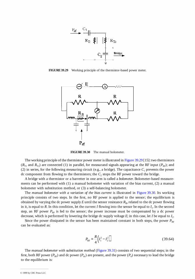
The working principle of the thermistor power meter is illustrated in Figure 39.29 [15]: two thermistors(RT1 and RT2) are connected (1) in parallel, for measurand signals appearing at the RF input (PRF); and(2) in series, for the following measuring circuit (e.g., a bridge). The capacitance C1 prevents the powerdc component from flowing to the thermistors; the C2 stops the RF power toward the bridge.

A bridge with a thermistor or a barretter in one arm is called a bolometer. Bolometer-based measure-ments can be performed with (1) a manual bolometer with variation of the bias current, (2) a manualbolometer with substitution method, or (3) a self-balancing bolometer.

The manual bolometer with a variation of the bias current is illustrated in Figure 39.30. Its workingprinciple consists of two steps. In the first, no RF power is applied to the sensor; the equilibrium isobtained by varying the dc power supply E until the sensor resistance RB, related to the dc power flowingin it, is equal to R. In this condition, let the current I flowing into the sensor be equal to I1. In the secondstep, an RF power PRF is fed to the sensor; the power increase must be compensated by a dc powerdecrease, which is performed by lowering the bridge dc supply voltage E; in this case, let I be equal to I2.

Since the power dissipated in the sensor has been maintained constant in both steps, the power PRF

can be evaluated as:

(39.64)

The manual bolometer with substitution method (Figure 39.31) consists of two sequential steps; in thefirst, both RF power (PRF) and dc power (Pdc) are present, and the power (Pd) necessary to lead the bridgeto the equilibrium is:

FIGURE 39.29 Working principle of the thermistor-based power meter.

FIGURE 39.30 The manual bolometer.

PR

I IRF = −( )4 1

222


(39.65)

During the second step, PRF is set to zero and an alternative voltage Vac is introduced in parallel to thedc power supply. In this case, the power Pd necessary to balance the bridge:

(39.66)

is obtained by varying vac.Since Pd is the same in both cases, the power supplied by the alternative generator is equal to PRF:

(39.67)

Equation 39.66 implies that the RF power can be obtained by a voltage measurement. The self-balancingbolometer (Figure 39.32) automatically supplies a dc voltage V to balance the voltage variations due tosensor resistance RB changes for an incident power PRF. At equilibrium, RB is equal to R and the RF powerwill then be:

(39.68)

FIGURE 39.31 Manual bolometer with substitution method.

FIGURE 39.32 Self-balancing bolometer.

P P Pd dc RF= +

P P Pd dc ac= +

P PV

RRF acac

2

= =4

PV

RRF =2

4


As mentioned above, the thermistor resistance depends on the surrounding temperature. This effectis compensated in an instrument based on two self-balancing bridges [15]. The RF power is input onlyto one of these, as shown in Figure 39.33.

The equilibrium voltages Vc and VRF feed a chopping and summing circuit, whose output Vc + VRF

goes to a voltage-to-time converter. This produces a pulse train V1, whose width is proportional to Vc +VRF. The chopping section also generates a signal with an amplitude proportional to Vc – VRF, and afrequency of a few kilohertz, which is further amplified. The signals V1 and V2 enter an electronic switchwhose output is measured by a medium value meter M. This measure is proportional to the RF powerbecause:

(39.69)

Owing to the differential structure of the two bolometers, this device is capable of performing RFpower measurements independent of the surrounding temperature. In addition, an offset calibration canbe carried out when PRF is null and Vc is equal to VRF.

These instruments can range from 10 mW to 1 µW and utilize sensors with frequency bandwidthsranging from 10 kHz to 100 GHz.

Thermocouple-Based Power Meters

Thermocouples [14] can be also used as RF power meters up to frequencies greater than 40 GHz. In thiscase, the resistor is generally a thin-film type. The sensitivity of a thermocouple can be expressed as theratio between the dc output amplitude and the input RF power. Typical values are 160 µV mW–1 forminimum power of about 1 µW.

The measure of voltages of about some tens of millivolts requires strong amplification, in that theamplifier does not have to introduce any offset. With this aim, a chopper microvoltmeter is utilized [16],as shown in the Figure 39.34.

The thermocouple output voltage Vdc is chopped at a frequency of about 100 Hz; the resulting squarewave is filtered of its mean value by the capacitor C and then input to an ac amplifier to further reduceoffset problems. A detector, synchronized to the chopper, and a low-pass filter transform the amplifiedsquare voltage in a dc voltage finally measured by a voltmeter.

FIGURE 39.33 Power meter based on two self-balancing bridges.

PV V V V

RP

V V

RRF

c RF c RF

RFc

2RF2

=+( ) −( )

⇒ = −4 4


Calorimetric Method

For high frequencies, a substitution technique based on a calorimetric method is utilized (Figure 39.35)[17]. First, the unknown radio frequency power PRF is sent to the measuring device t, which measuresthe equilibrium temperature. Then, once the calorimetric fluid has been cooled to its initial temperature,a dc power Pdc is applied to the device and regulated until the same temperature increase occurs in thesame time interval. In this way, a thermal energy equivalence is established between the known Pdc andthe measurand PRF .

A comparison version of the calorimetric method is also used for lower frequency power measurements(Figure 39.36). The temperature difference ∆T of a cooling fluid between the input (1) and the output(2) sections of a cooling element where the dissipated power to be measured P is determined. In thiscase, the power loss will correspond to P:

(39.70)

where Cp is the specific heat, ρ the density, and Q the volume flow, respectively, of the refreshing fluid.

FIGURE 39.34 Power meter with thermocouple-based sensor.

FIGURE 39.35 Calorimetric method based on a substitution technique.

FIGURE 39.36 Calorimetric method based on a comparison technique.

P C Q T= pρ ∆


Diode Sensor-Based Power Measurements

Very sensitive (up to 0.10 nW, –70 dBm), high-frequency (10 MHz to 20 GHz) power measurements arecarried out through a diode sensor by means of the circuit in Figure 39.37 [18]. In particular, accordingto a suitable selection of the components in this circuit, (1) true-average power measurements, or (2) peakpower measurements can be performed.

The basic concept underlying true-average power measurements exploits the nonlinear squared regionof the characteristic of a low-barrier Schottky diode (non-dashed area in Figure 39.38). In this region,the current flowing through the diode is proportional to the square of the applied voltage; thus, the diodeacts as a squared-characteristic sensor.

In the circuit of diode sensor-based wattmeters shown in Figure 39.37, the measurand vx, terminatedon the matching resistor Rm, is applied to the diode sensor Ds working in its squared region in order toproduce a corresponding output current ic in the bypass capacitor Cb. If Cb has been suitably selected,the voltage Vc between its terminals, measured by the voltmeter amplifier Va, is proportional to the averageof ic, i.e., to the average of the squares of instantaneous values of the input signal vx, and, hence, to thetrue average power.

In the true-average power measurement of nonsinusoidal waveforms having the biggest componentsat low frequency, such as radio-frequency AM (Amplitude Modulated), the value of Cb must also satisfyanother condition. The voltage vd on the diode must be capable of holding the diode switched-on intoconduction even for the smallest values of the signal. Otherwise, in the valleys of the modulation cycle,the high-frequency modulating source is disconnected by the back-biased diode and the measurementis therefore misleading.

On the other hand, for the same signal but for a different selection of the Cb value, the circuit can actas a peak detector for peak power measurements. As a matter of fact, the voltage vc on the bypass capacitorCb during the peak of the modulation cycle is so large that in the valleys, the high-frequency peaks are

FIGURE 39.37 Circuit of the diode sensor-based power measurement.

FIGURE 39.38 Characteristic of a low-barrier Schottky diode.


not capable of switching on the diode into conduction; thus, these peaks do not contribute to themeasured power level.

If higher power levels have to be measured (10 mW to 100 mW), the sensing diode is led to work outof the squared region into its linear region (dashed area in Figure 39.38). In this case, the advantage oftrue-average power measurements for distorted waveforms is lost; and for peak power measurements,since the diode input-output characteristic is nonlinear and the output is squared, spectral componentsdifferent from the fundamental introduce significant measuring errors.

Radiation Sensor-Based Power Measurements

Very high-frequency power measurements are usually carried out by measuring a radiant flux of anelectromagnetic radiation through a suitable sensor. In particular, semiconductor-based radiationmicrosensors have gained wider and wider diffusion [19], in that size reduction involves several well-known advantages such as greater portability, fewer materials, a wider range of applications, etc. One ofthe most familiar applications of radiation sensor-based power measurements is the detection of objectdisplacement. Furthermore, they are also commonly used for low-frequency power noninvasivemeasurements.

Radiation sensors can be classified according to the measurand class to which they are sensitive: nuclearparticles or electromagnetic radiations. In any case, particular sensors capable of detecting both nuclearparticles and electromagnetic radiations, such as gamma and X-rays, exist and are referred to as nucleonicdetectors.

In Table 39.1, the different types of radiation sensors utilized according to the decrease of the mea-surand wavelength from microwaves up to nuclear (X, gamma, and cosmic) rays are indicated.

In particular, microwave power radiation sensors are mainly used as noncontacting detectors relyingon ranging techniques using microwaves [20]. Shorter and longer (radar) wavelength microwave devicesare employed to detect metric and over-kilometer displacements, respectively.

Beyond applications analogous to microwave, power radiation infrared sensors also find use as contactdetectors. In particular, there are two types of infrared detectors: thermal and quantum. The thermaltype includes contacting temperature sensors such as thermocouples and thermopiles, as well as non-contacting pyroelectric detectors. On the other hand, the quantum type, although characterized by astrong wavelength dependence, has a faster response and includes photoconductive (spectral range:1 µm to 12 µm) and photovoltaic (0.5 µm to 5.5 µm) devices.

The main power radiation visible and ultraviolet sensors are photoconductive cells, photodiodes, andphototransistors. Photodiodes are widely used to detect the presence, the intensity, and the wavelengthof light or ultraviolet radiations. Compared to photoconductive cells, they are more sensitive, smaller,more stable and linear, and have lower response times. On the other hand, phototransistors are moresensitive to light.

At very low light levels, rather than silicon-based microsensors, nuclear radiation power microsensorsare needed. In this case, the most widespread devices are scintillation counters, solid-state detectors,plastic films, and thermoluminescent devices. The scintillation counter consists of an active material thatconverts the incident radiation to pulses of light, and a light-electric pulse converter. The active materialcan be a crystal, a plastic fluorine, or a liquid. The scintillator size varies greatly according to the radiationenergy, from thin solid films to large tanks of liquid to detect cosmic rays. A thin (5 µm) plastic

TABLE 39.1 Operating Field of Main Radiation Power Sensors

Visible andOperating field Microwave Infrared ultraviolet Nuclear rays(Wavelength) (1, 10–3 m) (10–3, 10–6 m) (10–6, 10–9 m) (10–8, 10–15 m)

Sensors Noncontactingdisplacement sensors

Pyroelectric, photoconductive, photovoltaic

Photoconductive, photovoltaic

Scintillation counters, plastic films, solid-state, thermolum


polycarbonate film or a thermoluminescent material (e.g., LiF) can measure the radiation power fallingon a surface. The film is mechanically damaged by the propagation of highly α–ionizing particles.Consequent etching of the film reveals tracks that can be observed and counted.

39.3 Pulse Power Measurements

Pulse waveforms are becoming more and more diffused in several fields such as telecommunications,power source applications, etc. The pulse power Pp is defined as the average power Pm in the pulse width:

(39.71)

where τd is the duty cycle of the pulse waveform (i.e., the pulse width divided by the waveform period).If the pulse width cannot be accurately defined (e.g., nonrectangular pulses in the presence of noise),the pulse power Pp becomes unmeaningful. In this case, the peak envelope power is introduced as themaximum of the instantaneous power detected on a time interval, including several periods of the pulsewaveform (but negligible with respect to the modulation period, in the case of PWM waveforms).

Several techniques are used to measure pulse power [21]. In particular, they can be classified accordingto the pulse frequency and the necessity for constraining real-time applications (i.e., measuring times, includ-ing a few of the modulation periods). For real-time, low-frequency applications (up to 100 kHz), thealgorithms mentioned in the above sections on wattmeters based on digital multipliers can be applied [9].

If constraining limits of real-time do not have to be satisfied, either digital or analog techniques canbe utilized. As far as the digital techniques are concerned, for high-frequency applications, if the mea-surand pulse waveform is stationary over several modulation periods, digital wattmeters based on equiv-alent sampling can be applied, with accuracies increasing according to measuring times. As far as theanalog techniques are concerned, three traditional methods are still valid: (1) average power per dutycycle, (2) integration-differentiation, and (3) dc/pulse power comparison.

A block diagram of an instrument measuring average power per duty cycle is illustrated in Figure 39.39.At first, the mean power of the measurand pulse signal, terminated on a suitable load, is measured bymeans of an average power meter; then, the pulse width and the pulse waveform period are measuredby a digital counter. Finally, the power is obtained by means of Equation 39.71.

The integration-differentiation technique is based on a barretter sensor capable of integrating themeasurand, and on a conditioning and differentiating circuit to obtain a voltage signal proportional tothe measurand power. The signal is input to the barretter sensor, having a thermal constant such thatthe barretter resistance will correspond to the integral of the input. The barretter is mounted as an armof a conditioning Wheatstone bridge; in this way, the barretter resistance variations are transformed intovoltage variations, and an integrated voltage signal is obtained as an output of the bridge detecting arm.

FIGURE 39.39 Block diagram of an instrument measuring average power per duty cycle.

PP

pm

d

=τ


This signal, suitably integrated to reach a voltage signal proportional to the output, is detected by a peakvoltmeter calibrated in power. Analogously to the selection of the time constant of an RC integratingcircuit, attention must be paid to the thermal constant selection of the barretter in order to attain thedesired accuracy in the integration. With respect to the measurand pulse period, a very long thermalconstant will give rise to insufficient sensitivity. On the other hand, a very short constant approachingthe pulse duration will give rise to insufficient accuracy.

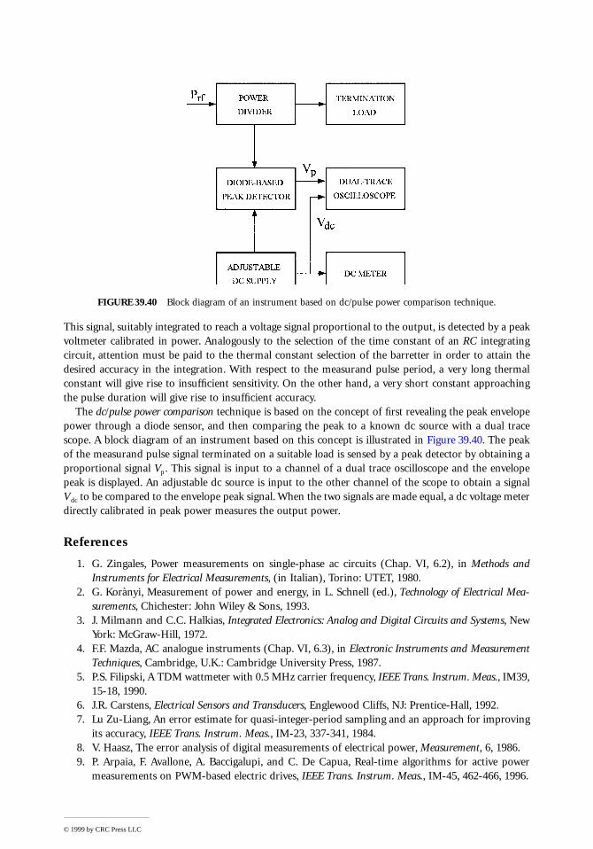
The dc/pulse power comparison technique is based on the concept of first revealing the peak envelopepower through a diode sensor, and then comparing the peak to a known dc source with a dual tracescope. A block diagram of an instrument based on this concept is illustrated in Figure 39.40. The peakof the measurand pulse signal terminated on a suitable load is sensed by a peak detector by obtaining aproportional signal Vp. This signal is input to a channel of a dual trace oscilloscope and the envelopepeak is displayed. An adjustable dc source is input to the other channel of the scope to obtain a signalVdc to be compared to the envelope peak signal. When the two signals are made equal, a dc voltage meterdirectly calibrated in peak power measures the output power.

References

1. G. Zingales, Power measurements on single-phase ac circuits (Chap. VI, 6.2), in Methods andInstruments for Electrical Measurements, (in Italian), Torino: UTET, 1980.

2. G. Korànyi, Measurement of power and energy, in L. Schnell (ed.), Technology of Electrical Mea-surements, Chichester: John Wiley & Sons, 1993.

3. J. Milmann and C.C. Halkias, Integrated Electronics: Analog and Digital Circuits and Systems, NewYork: McGraw-Hill, 1972.

4. F.F. Mazda, AC analogue instruments (Chap. VI, 6.3), in Electronic Instruments and MeasurementTechniques, Cambridge, U.K.: Cambridge University Press, 1987.

5. P.S. Filipski, A TDM wattmeter with 0.5 MHz carrier frequency, IEEE Trans. Instrum. Meas., IM39,15-18, 1990.

6. J.R. Carstens, Electrical Sensors and Transducers, Englewood Cliffs, NJ: Prentice-Hall, 1992.7. Lu Zu-Liang, An error estimate for quasi-integer-period sampling and an approach for improving

its accuracy, IEEE Trans. Instrum. Meas., IM-23, 337-341, 1984.8. V. Haasz, The error analysis of digital measurements of electrical power, Measurement, 6, 1986.9. P. Arpaia, F. Avallone, A. Baccigalupi, and C. De Capua, Real-time algorithms for active power

measurements on PWM-based electric drives, IEEE Trans. Instrum. Meas., IM-45, 462-466, 1996.

FIGURE 39.40 Block diagram of an instrument based on dc/pulse power comparison technique.


10. X. Dai and R. Gretsch, Quasi-synchronous sampling algorithm and its applications, IEEE Trans.Instrum. Meas., IM-43, 204-209, 1994.

11. M. Bellanger, Digital Processing of Signals: Theory and Practice, Chichester: John Wiley & Sons, 1984.12. M. Bertocco, C. Offelli, and D. Petri, Numerical algorithms for power measurements, Europ. Trans.

Electr. Power, ETEP 3, 91-101, 1993.13. G. Zingales, Measurements on steady-state circuits (Chap. VI), in Methods and Instruments for

Electrical Measurements, (In Italian), Torino: UTET, 1980.14. H.N. Norton, Thermometers (Chap. 19), in Handbook of Transducers, Englewood Cliffs, NJ: Pren-

tice-Hall, 1989.15. Anonymous, Thermistor mounts and instrumentation (Chap. II), in Fundamental of RF and Micro-

wave Power Measurements, Application Note 64-1, Hewlett Packard, 1978.16. R.E. Pratt, Power measurements (15.1–15.16), in C.F. Coombs, (ed.), in Handbook of Electronic

Instruments, New York: McGraw-Hill, 1995.17. F. F. Mazda, High-frequency power measurements (Chap. VIII, 8.4), in Electronic Instruments and

Measurement Techniques, Cambridge: Cambridge University Press, 1987.18. Anonymous, Diode detector power sensors and instrumentation (Chap. IV), in Fundamental of

RF and Microwave Power Measurements, Application Note 64-1, Hewlett Packard, 1978.19. J.W. Gardner, Microsensors: Principles and Applications, Chichester: John Wiley & Sons, 1994.20. H.N. Norton, Radiation pyrometers (Chap. 20), in Handbook of Transducers, Englewood Cliffs, NJ:

Prentice-Hall, 1989.21. F.F. Mazda, Pulse power measurement (Chap. VIII, 8.5), in Electronic Instruments and Measurement

Techniques, Cambridge, U.K.: Cambridge University Press, 1987.

Further Information

F.K. Harris, The Measurement of Power (Chap. XI), in Electrical Measurements, Huntington, NY: R.E.Krieger Publishing, 1975; a clear reference for line-frequency power measurements.

Anonymous, Fundamental of RF and Microwave Power Measurements, Application Note 64-1, HewlettPackard, 1978; though not very recent, is a valid and comprehensive reference for main principlesof high-frequency power measurements.

J.J. Clarke and J.R. Stockton, Principles and theory of wattmeters operating on the basis of regularlyspaced sample pairs, J. Phys. E. Sci. Instrum., 15, 645-652, 1982; gives basics of synchronoussampling for digital wattmeters.

T.S. Rathore, Theorems on power, mean and RMS values of uniformly sampled periodic signals, IEEProc. Pt. A, 131, 598-600, 1984; provides fundamental theorems for effective synchronous samplingwattmeters.

J.K. Kolanko, Accurate measurement of power, energy, and true RMS voltage using synchronous counting,IEEE Trans. Instrum. Meas., IM-42, 752–754, 1993; provides information on the implementationof a synchronous dual-slope wattmeter.

G.N. Stenbakken, A wideband sampling wattmeter, IEEE Trans. Power App. Syst., PAS-103, 2919-2925,1984; gives basics of asynchronous sampling-based wattmeters and criteria for computing uncer-tainty in time domain.

F. Avallone, C. De Capua, and C. Landi, Measurement station performance optimization for testing onhigh efficiency variable speed drives, Proc. IEEE IMTC/96 (Brussels, Belgium), 1098–1103, 1996;proposes an analytical model of uncertainty arising from power measurement systems workingunder highly distorted conditions.

F. Avallone, C. De Capua, and C. Landi, Metrological performance improvement for power measurementson variable speed drives, Measurement, 21, 1997, 17-24; shows how compute uncertainty of mea-suring chain components for power measurements under highly distorted conditions.


F. Avallone, C. De Capua, and C. Landi, Measurand reconstruction techniques applied to power mea-surements on high efficiency variable speed drives, Proc. of XIV IMEKO World Congress (Tampere,Fi), 1997; proposes a technique to improve accuracy of power measurements under highly distortedconditions.

F. Avallone, C. De Capua, and C. Landi, A digital technique based on real-time error compensation forhigh accuracy power measurement on variable speed drives, Proc. of IEEE IMTC/97 (Ottawa,Canada), 1997; reports about a real-time technique for error compensation of transducers workingunder highly distorted conditions.

J.C. Montano, A. Lopez, M. Castilla, and J. Gutierrrez, DSP-based algorithm for electric power measure-ment, IEE Proc. Pt.A, 140, 485–490, 1993; describes a Goertzel FFT-based algorithm to computepower under nonsinusoidal conditions.

S.L. Garverick, K. Fujino, D.T. McGrath, and R.D. Baertsch, A programmable mixed-signal ASIC forpower metering, IEEE J. Solid State Circuits, 26, 2008–2015, 1991; reports about a programmablemixed analog-digital integrated circuit based on six first-order sigma-delta ADCs, a bit serial DSP,and a byte-wide static RAM for power metering.

G. Bucci, P. D’Innocenzo, and C. Landi, A modular high-speed dsp-based data acquisition apparatus foron-line quality analysis on power systems under non-sinusoidal conditions, Proc. of 9th IMEKOTC4 Int. Sym. (Budapest, Hungary), 286–289, 1996; shows the strategy of measurement systemdesign for power measurements under non-sinusoidal conditions.

K.K. Clarke and D.T. Hess, A 1000 A/20 kV/25 kHz-500 kHz volt-ampere-wattmeter for loads with powerfactors from 0.001 to 1.00, IEEE Trans. Instrum. Meas., IM-45, 142-145, 1996; provides informationon the implementation of a instrument to perform an accurate measurement of currents (1 A to1000 A), voltages (100 V to 20 kV), and powers (100 W to 20 MW) over the frequency range from25 kHz to 500 kHz.

P. Arpaia, G. Betta, A. Langella, and M. Vanacore, An Expert System for the Optimum Design ofMeasurement Systems, IEE Proc. (Pt. A), 142, 330–336, 1995; reports about an Artificial Intelligencetool for the automatic design of power measuring systems.

In any case, IEEE Transactions on Instrumentation and Measurement and Measurement journals providecurrent research on power measurements.


Documents

P. Arpaia, et. al.. Power Measurement. Copyright 2000 …etc.unitbv.ro/~olteanu/Tehnici de masurare in tc/Mas. P.pdfIn this chapter, the concept of electric power is ﬁrst introduced,