Overview of Multi-Frequency EPRfajer/Fajerlab/LinkedDocuments/Ralph Weber.pdf · Overview of Multi-Frequency EPR ... but the improvement in sensitivity is tempered by the decrease

Overview of Multi-Frequency EPR

Overview of Multi-Frequency EPRMost EPR (Electron Paramagnetic Resonance) experiments are performed atX-band (9-10 GHz). Many factors contribute to the choice of this frequency.One factor is the availability of components: with the development ofRADAR and the end of World War II, there was a glut of surplus X-band mil-itary microwave equipment available to the early EPR pioneers.

In addition to historic factors, convenience plays an important role. The mag-netic field requirements for X-band are usually satisfied easily by electro-magnets. The 3 cm wavelength ensures convenient sample sizes and samplehandling.

A third consideration is sensitivity. As the Boltzmann factor and sample sizeincrease, they increase the spectrometer’s sensitivity. Alas, the two factors arenot independent. The Boltzmann factor increases with increasing frequency,but the improvement in sensitivity is tempered by the decrease in sample sizewith increasing frequency. If you have sufficient sample, albeit at a low con-centration, X-band often offers the best sensitivity.

These factors lead to the almost universal acceptance that EPR is performedat X-band. Given all the advantages of X-band EPR, why would researcherswish to perform experiments at lower or higher frequencies? Performing EPRspectroscopy at multiple frequencies sheds additional light on the propertiesof the sample. If we were to see everything only in black and white, we wouldmiss all the extra information that color vision affords us. In an analogousfashion, if we were to measure our samples at X-band only (black and white),we would miss the complete picture that other microwave frequencies (colorvision) could offer us.

The appearance of EPR spectra depends strongly on the interplay of magneticfield dependent and magnetic field independent interactions. By operating atseveral frequencies, we are able to resolve the contributions from the twotypes of interactions and thereby obtain unambiguous answers to the ques-tions posed by our sample.

In this overview we shall consider the advantages of going higher or lower infrequencies compared to X-band. We shall explore the benefits from the com-plementary information offered by high and low frequencies. Finally, themethodology and technical aspects of multi-frequency EPR spectroscopy willbe introduced.

Some Preliminary Definitions

2

Some Preliminary Definitions 1This overview will make use of certain terms that may not be commonknowledge for many people using EPR spectroscopy. Here we shall definesome of those terms.

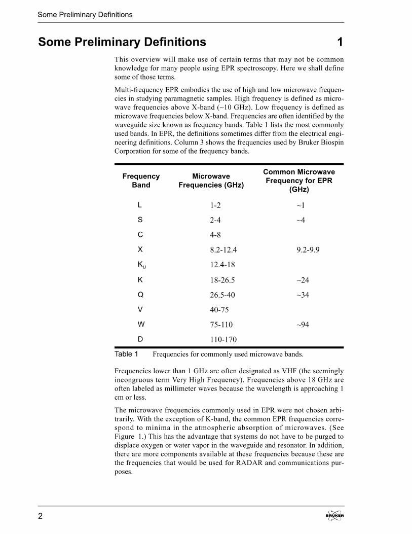
Multi-frequency EPR embodies the use of high and low microwave frequen-cies in studying paramagnetic samples. High frequency is defined as micro-wave frequencies above X-band (~10 GHz). Low frequency is defined asmicrowave frequencies below X-band. Frequencies are often identified by thewaveguide size known as frequency bands. Table 1 lists the most commonlyused bands. In EPR, the definitions sometimes differ from the electrical engi-neering definitions. Column 3 shows the frequencies used by Bruker BiospinCorporation for some of the frequency bands.

Frequencies lower than 1 GHz are often designated as VHF (the seeminglyincongruous term Very High Frequency). Frequencies above 18 GHz areoften labeled as millimeter waves because the wavelength is approaching 1cm or less.

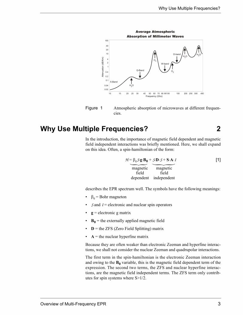
The microwave frequencies commonly used in EPR were not chosen arbi-trarily. With the exception of K-band, the common EPR frequencies corre-spond to minima in the atmospheric absorption of microwaves. (SeeFigure 1.) This has the advantage that systems do not have to be purged todisplace oxygen or water vapor in the waveguide and resonator. In addition,there are more components available at these frequencies because these arethe frequencies that would be used for RADAR and communications pur-poses.

Frequency Band

Microwave Frequencies (GHz)

Common Microwave Frequency for EPR

(GHz)

L 1-2 ~1

S 2-4 ~4

C 4-8

X 8.2-12.4 9.2-9.9

Ku 12.4-18

K 18-26.5 ~24

Q 26.5-40 ~34

V 40-75

W 75-110 ~94

D 110-170

Table 1 Frequencies for commonly used microwave bands.

Why Use Multiple Frequencies?

Overview of Multi-Frequency EPR 3

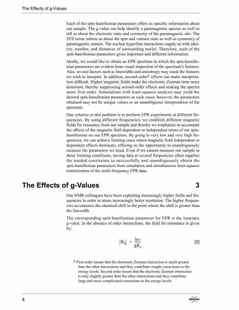
Why Use Multiple Frequencies? 2In the introduction, the importance of magnetic field dependent and magneticfield independent interactions was briefly mentioned. Here, we shall expandon this idea. Often, a spin-hamiltonian of the form:

H = �eS�g�B0 + S�D�S + S�A�I [1]

describes the EPR spectrum well. The symbols have the following meanings:

• �e = Bohr magneton

• S and I = electronic and nuclear spin operators

• g = electronic g matrix

• B0 = the externally applied magnetic field

• D = the ZFS (Zero Field Splitting) matrix

• A = the nuclear hyperfine matrix

Because they are often weaker than electronic Zeeman and hyperfine interac-tions, we shall not consider the nuclear Zeeman and quadrupolar interactions.

The first term in the spin-hamiltonian is the electronic Zeeman interactionand owing to the B0 variable, this is the magnetic field dependent term of theexpression. The second two terms, the ZFS and nuclear hyperfine interac-tions, are the magnetic field independent terms. The ZFS term only contrib-utes for spin systems where S>1/2.

Figure 1 Atmospheric absorption of microwaves at different frequen-cies.

10 15 20 25 30 40 50 60 70 80 90100 150 200 250 300 400

100

40

20

10

4

2

1

0.4

0.2

0.1

0.04

0.02

Atte

nuat

ion

(dB

/Km

)

Frequency (Ghz)

X-Band

Q-Band

W-band

D-band

H O2

H O2H O2

O2

O2

Average AtmosphericAbsorption of Millimeter Waves

} }

magneticfield

dependent

magneticfield

independent

The Effects of g-Values

4

Each of the spin-hamiltonian parameters offers us specific information aboutour sample. The g-value can help identify a paramagnetic species as well astell us about the electronic state and symmetry of the paramagnetic site. TheZFS terms inform us about the spin and valence state as well as symmetry ofparamagnetic centers. The nuclear hyperfine interactions supply us with iden-tity, number, and distances of surrounding nuclei. Therefore, each of thespin-hamiltonian parameters gives important and different information.

Ideally, we would like to obtain an EPR spectrum in which the spin-hamilto-nian parameters are evident from visual inspection of the spectrum’s features.Alas, several factors such as linewidths and anisotropy may mask the featureswe wish to interpret. In addition, second-order* effects can make interpreta-tion difficult. Higher magnetic fields make the electronic Zeeman term moredominant, thereby suppressing second-order effects and making the spectramore first-order. Simulations with least-squares analysis may yield thedesired spin-hamiltonian parameters in such cases, however, the parametersobtained may not be unique values or an unambiguous interpretation of thespectrum.

One solution to this problem is to perform EPR experiments at different fre-quencies. By using different frequencies, we establish different magneticfields for resonance from our sample and thereby we emphasize or accentuatethe effects of the magnetic field dependent or independent terms of our spin-hamiltonian on our EPR spectrum. By going to very low and very high fre-quencies, we can achieve limiting cases where magnetic field independent ordependent effects dominate, offering us the opportunity to unambiguouslymeasure the parameters we need. Even if we cannot measure our sample inthese limiting conditions, having data at several frequencies often suppliesthe needed constraints to successfully and unambiguously obtain thespin-hamiltonian parameters from simulation and simultaneous least-squaresminimization of the multi-frequency EPR data.

The Effects of g-Values 3Our NMR colleagues have been exploiting increasingly higher fields and fre-quencies in order to attain increasingly better resolution. The higher frequen-cies accentuates the chemical shift to the point where the shift is greater thanthe linewidth.

The corresponding spin-hamiltonian parameter for EPR is the isotropicg-value. In the absence of other interactions, the field for resonance is givenby:

[2]

* First order means that the electronic Zeeman interaction is much greater than the other interactions and they contribute simple corrections to the energy levels. Second order means that the electronic Zeeman interaction is only slightly greater than the other interactions and they contribute large and more complicated corrections to the energy levels.

B0h�g�e--------=



where h is Planck’s constant, � is the microwave frequency, g is the isotropicg-value, and �e is the Bohr magneton. If we were to have two paramagneticspecies in our sample with a small g-value difference of �g, the difference infields for resonance, �B, is approximately proportional to the microwave fre-quency:

. [3]

If �B can be made greater than the linewidth by increasing the microwavefrequency, we can unambiguously identify the two species in our sample.

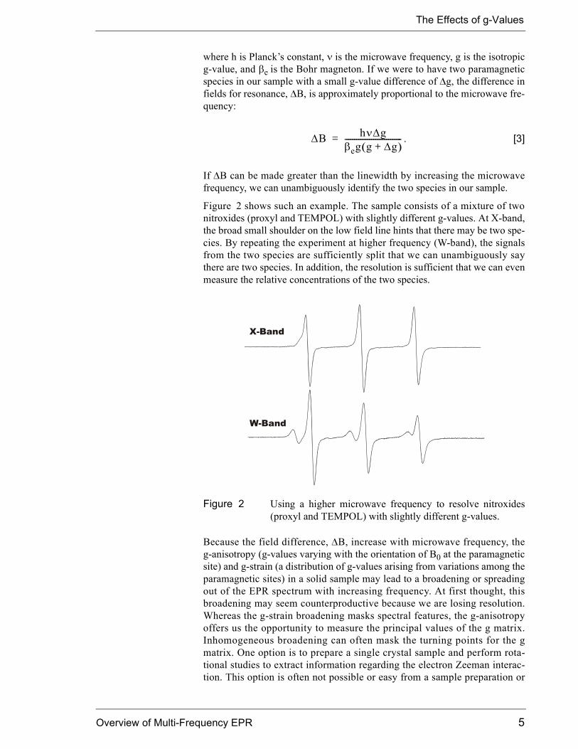
Figure 2 shows such an example. The sample consists of a mixture of twonitroxides (proxyl and TEMPOL) with slightly different g-values. At X-band,the broad small shoulder on the low field line hints that there may be two spe-cies. By repeating the experiment at higher frequency (W-band), the signalsfrom the two species are sufficiently split that we can unambiguously saythere are two species. In addition, the resolution is sufficient that we can evenmeasure the relative concentrations of the two species.

Because the field difference, �B, increase with microwave frequency, theg-anisotropy (g-values varying with the orientation of B0 at the paramagneticsite) and g-strain (a distribution of g-values arising from variations among theparamagnetic sites) in a solid sample may lead to a broadening or spreadingout of the EPR spectrum with increasing frequency. At first thought, thisbroadening may seem counterproductive because we are losing resolution.Whereas the g-strain broadening masks spectral features, the g-anisotropyoffers us the opportunity to measure the principal values of the g matrix.Inhomogeneous broadening can often mask the turning points for the gmatrix. One option is to prepare a single crystal sample and perform rota-tional studies to extract information regarding the electron Zeeman interac-tion. This option is often not possible or easy from a sample preparation or

Figure 2 Using a higher microwave frequency to resolve nitroxides(proxyl and TEMPOL) with slightly different g-values.

�B h��g�eg g �g+� �------------------------------=

W-Band

X-Band


6

measurement time standpoint. By performing experiments at higher frequen-cies, we can emphasize and accentuate the field dependent term, the electronZeeman term, so that it dominates over the inhomogeneous linewidth.

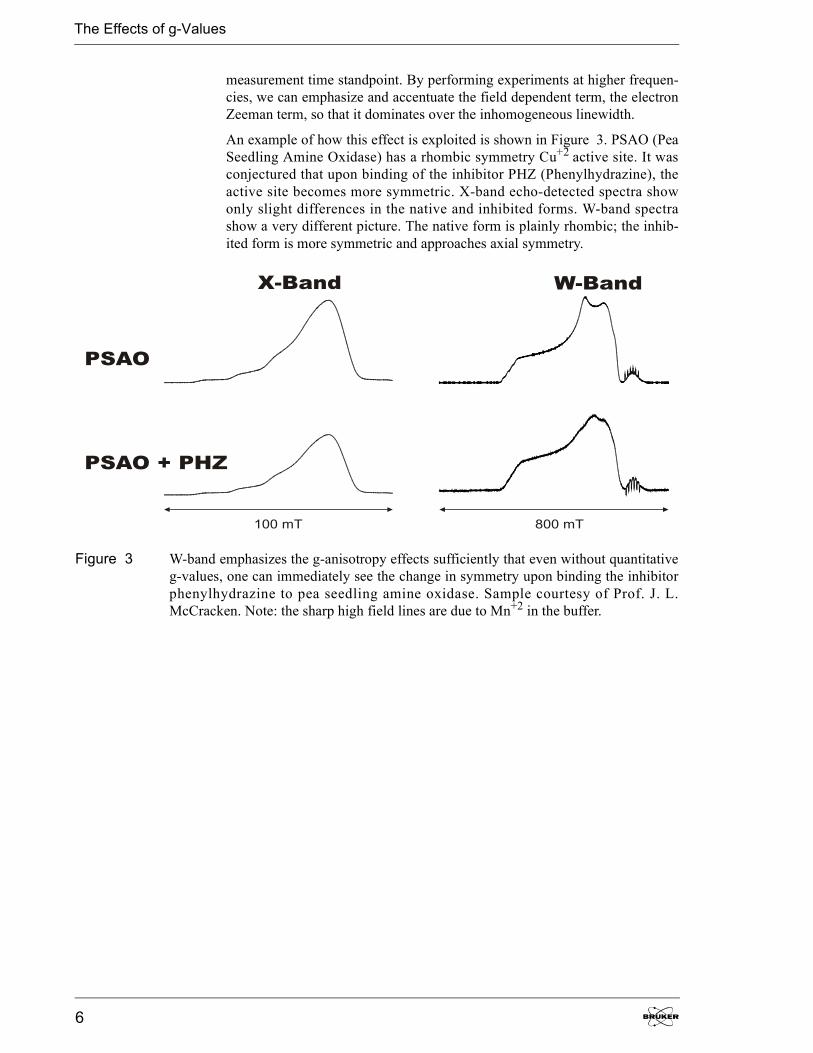
An example of how this effect is exploited is shown in Figure 3. PSAO (PeaSeedling Amine Oxidase) has a rhombic symmetry Cu+2 active site. It wasconjectured that upon binding of the inhibitor PHZ (Phenylhydrazine), theactive site becomes more symmetric. X-band echo-detected spectra showonly slight differences in the native and inhibited forms. W-band spectrashow a very different picture. The native form is plainly rhombic; the inhib-ited form is more symmetric and approaches axial symmetry.

Figure 3 W-band emphasizes the g-anisotropy effects sufficiently that even without quantitativeg-values, one can immediately see the change in symmetry upon binding the inhibitorphenylhydrazine to pea seedling amine oxidase. Sample courtesy of Prof. J. L.McCracken. Note: the sharp high field lines are due to Mn+2 in the buffer.

W-BandX-Band

PSAO

PSAO + PHZ

100 mT 800 mT

The Effects of Nuclear Hyperfine Couplings


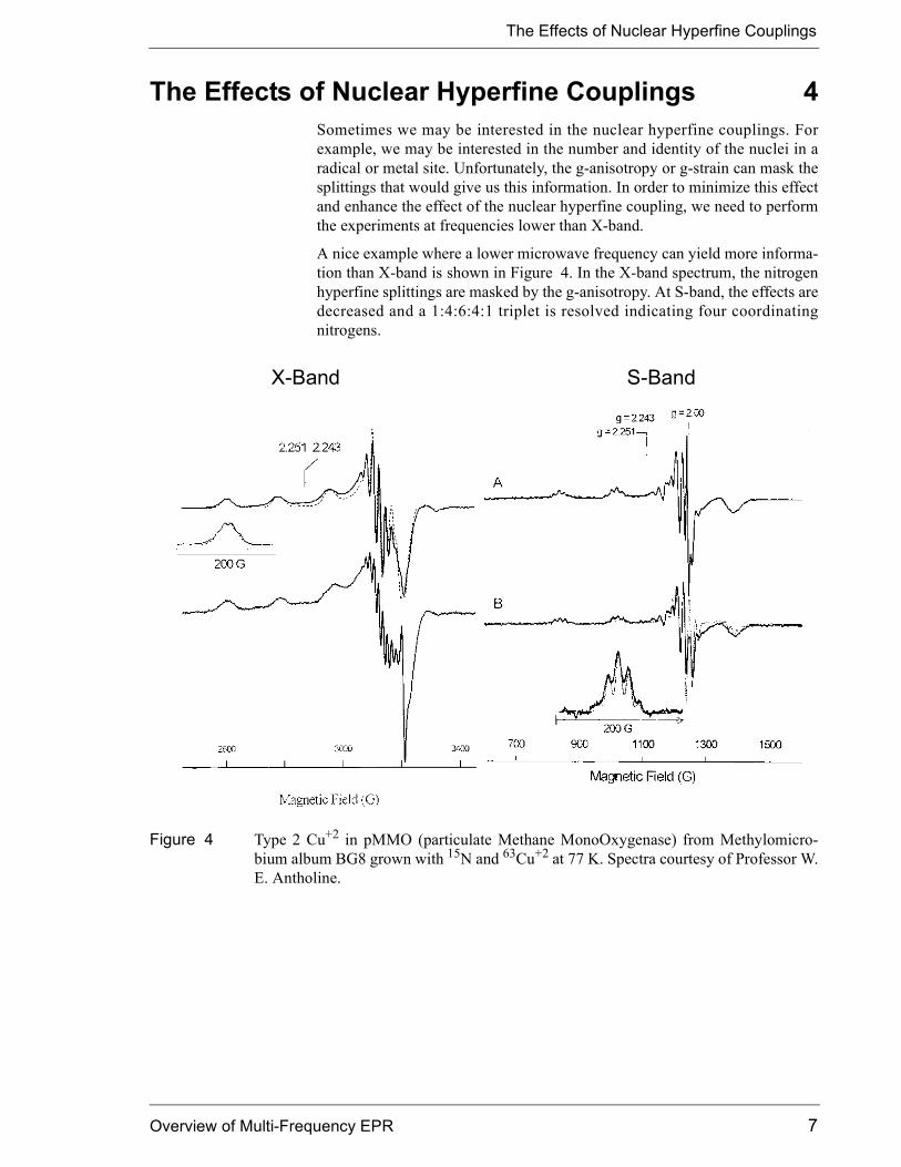
The Effects of Nuclear Hyperfine Couplings 4Sometimes we may be interested in the nuclear hyperfine couplings. Forexample, we may be interested in the number and identity of the nuclei in aradical or metal site. Unfortunately, the g-anisotropy or g-strain can mask thesplittings that would give us this information. In order to minimize this effectand enhance the effect of the nuclear hyperfine coupling, we need to performthe experiments at frequencies lower than X-band.

A nice example where a lower microwave frequency can yield more informa-tion than X-band is shown in Figure 4. In the X-band spectrum, the nitrogenhyperfine splittings are masked by the g-anisotropy. At S-band, the effects aredecreased and a 1:4:6:4:1 triplet is resolved indicating four coordinatingnitrogens.

Figure 4 Type 2 Cu+2 in pMMO (particulate Methane MonoOxygenase) from Methylomicro-bium album BG8 grown with 15N and 63Cu+2 at 77 K. Spectra courtesy of Professor W.E. Antholine.

X-Band S-Band

The Effects of Nuclear Hyperfine Couplings

8

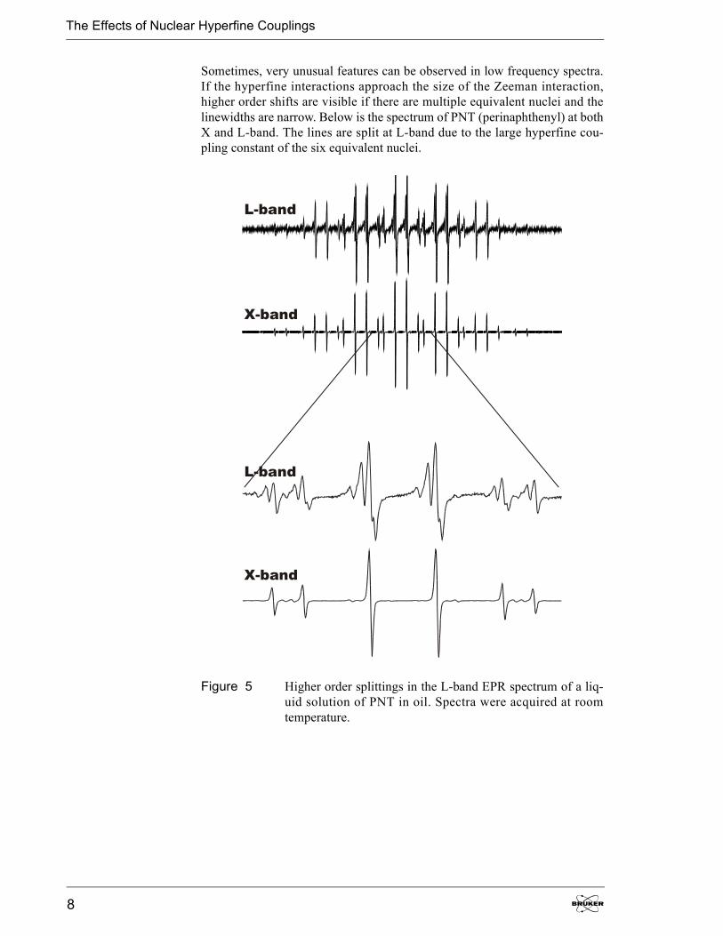
Sometimes, very unusual features can be observed in low frequency spectra.If the hyperfine interactions approach the size of the Zeeman interaction,higher order shifts are visible if there are multiple equivalent nuclei and thelinewidths are narrow. Below is the spectrum of PNT (perinaphthenyl) at bothX and L-band. The lines are split at L-band due to the large hyperfine cou-pling constant of the six equivalent nuclei.

Figure 5 Higher order splittings in the L-band EPR spectrum of a liq-uid solution of PNT in oil. Spectra were acquired at roomtemperature.

L-band

X-band

X-band

L-band

The Effects of Zero Field Splittings


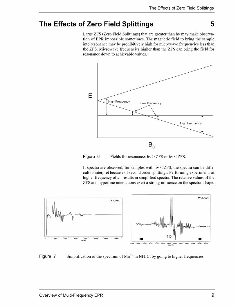
The Effects of Zero Field Splittings 5Large ZFS (Zero Field Splittings) that are greater than h� may make observa-tion of EPR impossible sometimes. The magnetic field to bring the sampleinto resonance may be prohibitively high for microwave frequencies less thanthe ZFS. Microwave frequencies higher than the ZFS can bring the field forresonance down to achievable values.

If spectra are observed, for samples with h� < ZFS, the spectra can be diffi-cult to interpret because of second order splittings. Performing experiments athigher frequency often results in simplified spectra. The relative values of theZFS and hyperfine interactions exert a strong influence on the spectral shape.

Figure 6 Fields for resonance: h� > ZFS or h� < ZFS.

E

B0

High Frequency Low Frequency

High Frequency

Figure 7 Simplification of the spectrum of Mn+2 in NH4Cl by going to higher frequencies.

X-bandW-band

4D

The Effects of Zero Field Splittings

10

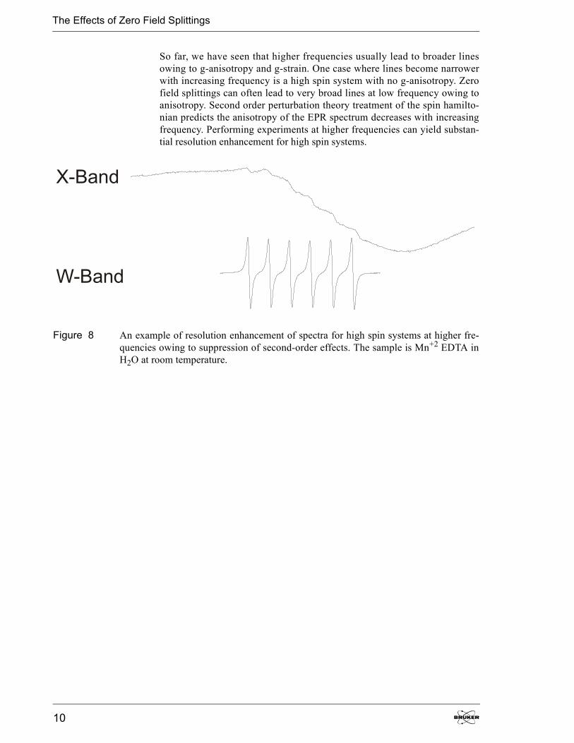
So far, we have seen that higher frequencies usually lead to broader linesowing to g-anisotropy and g-strain. One case where lines become narrowerwith increasing frequency is a high spin system with no g-anisotropy. Zerofield splittings can often lead to very broad lines at low frequency owing toanisotropy. Second order perturbation theory treatment of the spin hamilto-nian predicts the anisotropy of the EPR spectrum decreases with increasingfrequency. Performing experiments at higher frequencies can yield substan-tial resolution enhancement for high spin systems.

Figure 8 An example of resolution enhancement of spectra for high spin systems at higher fre-quencies owing to suppression of second-order effects. The sample is Mn+2 EDTA inH2O at room temperature.

W-Band

X-Band

Relaxation Times


Relaxation Times 6Many mechanisms can contribute to relaxation times. Commonly, tempera-ture studies of relaxation rates are performed to distinguish between differentmechanisms, but such studies do not always yield an unambiguous answer.Some mechanisms for T1 (spin lattice relaxation) are frequency independentsuch as the Raman or local-mode process and some are frequency dependentsuch as the direct or thermally activated process. By studying both the fre-quency and temperature dependence, sufficient constraints are placed on theresults to identify dominant relaxation mechanisms. For example, T1 forTEMPOL in 4-OH-2,2,6,6 tetramethyl-piperidinol at temperatures higherthan 160 K exhibits contributions from a Raman process and either localmode or thermally activated process. Because T1 is frequency dependent, wecan conclude that a thermally activated process is contributing to T1.

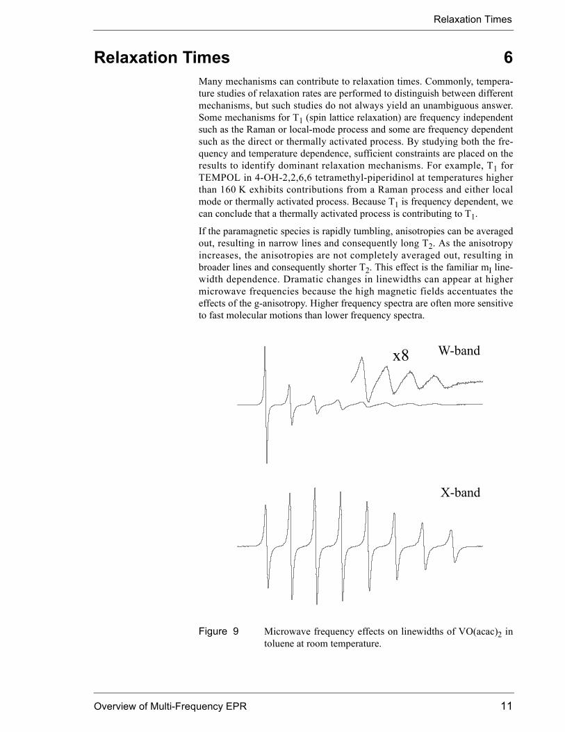
If the paramagnetic species is rapidly tumbling, anisotropies can be averagedout, resulting in narrow lines and consequently long T2. As the anisotropyincreases, the anisotropies are not completely averaged out, resulting inbroader lines and consequently shorter T2. This effect is the familiar mI line-width dependence. Dramatic changes in linewidths can appear at highermicrowave frequencies because the high magnetic fields accentuates theeffects of the g-anisotropy. Higher frequency spectra are often more sensitiveto fast molecular motions than lower frequency spectra.

Figure 9 Microwave frequency effects on linewidths of VO(acac)2 intoluene at room temperature.

X-band

W-bandx8

The Role of Sample Properties & Sensitivity

12

The Role of Sample Properties & Sensitivity 7Quite often, we do not have a choice about the size, concentration, or dielec-tric properties of our samples. These properties play an important role in thechoice of microwave frequency.

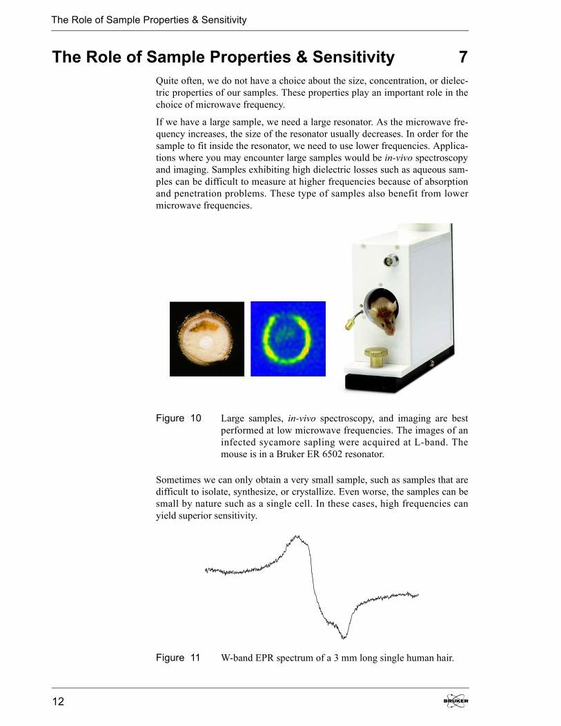
If we have a large sample, we need a large resonator. As the microwave fre-quency increases, the size of the resonator usually decreases. In order for thesample to fit inside the resonator, we need to use lower frequencies. Applica-tions where you may encounter large samples would be in-vivo spectroscopyand imaging. Samples exhibiting high dielectric losses such as aqueous sam-ples can be difficult to measure at higher frequencies because of absorptionand penetration problems. These type of samples also benefit from lowermicrowave frequencies.

Sometimes we can only obtain a very small sample, such as samples that aredifficult to isolate, synthesize, or crystallize. Even worse, the samples can besmall by nature such as a single cell. In these cases, high frequencies canyield superior sensitivity.

Figure 10 Large samples, in-vivo spectroscopy, and imaging are bestperformed at low microwave frequencies. The images of aninfected sycamore sapling were acquired at L-band. Themouse is in a Bruker ER 6502 resonator.

Figure 11 W-band EPR spectrum of a 3 mm long single human hair.

Technology and Methodology


Technology and Methodology 8Each of the different microwave frequency bands requires different technol-ogy and techniques in order to successfully perform EPR experiments. Themicrowave frequency greatly effects the choice of resonator, transmissionline, sample tube, and magnet.

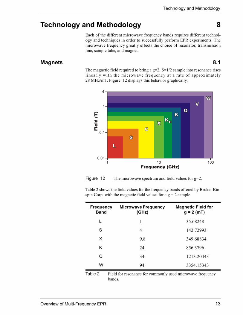
Magnets 8.1The magnetic field required to bring a g=2, S=1/2 sample into resonance riseslinearly with the microwave frequency at a rate of approximately28 MHz/mT. Figure 12 displays this behavior graphically.

Table 2 shows the field values for the frequency bands offered by Bruker Bio-spin Corp. with the magnetic field values for a g = 2 sample.

Figure 12 The microwave spectrum and field values for g=2.

Frequency Band

Microwave Frequency (GHz)

Magnetic Field for g = 2 (mT)

L 1 35.68248

S 4 142.72993

X 9.8 349.68834

K 24 856.3796

Q 34 1213.20443

W 94 3354.15343

Table 2 Field for resonance for commonly used microwave frequency bands.

1

4

10010

0.1

10.01

Frequency (GHz)

Fiel

d (T

)


14

Given enough electricity, cooling water, and floor strength, an iron electro-magnet can supply magnetic fields up to 2T.

For fields higher than 2 T, a superconducting magnet is required. Their highinductance make them difficult to sweep quickly. Therefore, these magnetsare often fitted with some room temperature resistive coils as well, so that onecan quickly and conveniently sweep the magnet about its persistent field.

Figure 13 An iron electromagnet.

Figure 14 A Bruker Hybrid3 superconducting magnet fitted with roomtemperature resistive sweep coils.



Wavelength & Sample Size 8.2The wavelength decreases with increasing frequency in the following man-ner:

[4]

where � is the wavelength in mm, � is the microwave frequency in Hz, and cis the speed of light, 2.998x1011 mm/s. Table 3 shows the wavelengths for thefrequency bands offered by Bruker Biospin Corp.

Because the size of the resonator is influenced by the wavelength (SeeSection 7.), longer wavelengths allow you to use larger samples.

Frequency Band

Microwave Frequency (GHz) Wavelength (mm)

L 1 300

S 4 75

X 9.8 30

K 24 12.5

Q 34 10

W 94 3

Table 3 Wavelengths for commonly used microwave frequency bands.

Frequency Band


Sample Tube O.D. (mm)

L 1 30

X 9.8 4

Q 34 2

W 94 0.9

Table 4 Sample tube sizes for commonly used microwave frequency bands.

�c�---=


16

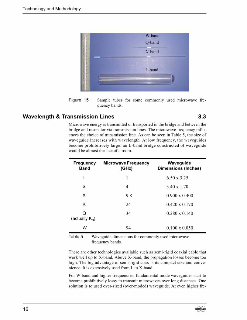
Wavelength & Transmission Lines 8.3Microwave energy is transmitted or transported in the bridge and between thebridge and resonator via transmission lines. The microwave frequency influ-ences the choice of transmission line. As can be seen in Table 5, the size ofwaveguide increases with wavelength. At low frequency, the waveguidesbecome prohibitively large: an L-band bridge constructed of waveguidewould be almost the size of a room.

There are other technologies available such as semi-rigid coaxial cable thatwork well up to X-band. Above X-band, the propagation losses become toohigh. The big advantage of semi-rigid coax is its compact size and conve-nience. It is extensively used from L to X-band.

For W-band and higher frequencies, fundamental mode waveguides start tobecome prohibitively lossy to transmit microwaves over long distances. Onesolution is to used over-sized (over-moded) waveguide. At even higher fre-

Figure 15 Sample tubes for some commonly used microwave fre-quency bands.

W-bandQ-band

X-band

L-band

Frequency Band


Waveguide Dimensions (Inches)

L 1 6.50 x 3.25

S 4 3.40 x 1.70

X 9.8 0.900 x 0.400

K 24 0.420 x 0.170

Q (actually Ka)

34 0.280 x 0.140

W 94 0.100 x 0.050

Table 5 Waveguide dimensions for commonly used microwave frequency bands.



quencies (> 140 GHz) quasi-optical techniques such as corrugated guides,mirrors, and lenses offer low-loss microwave propagation.

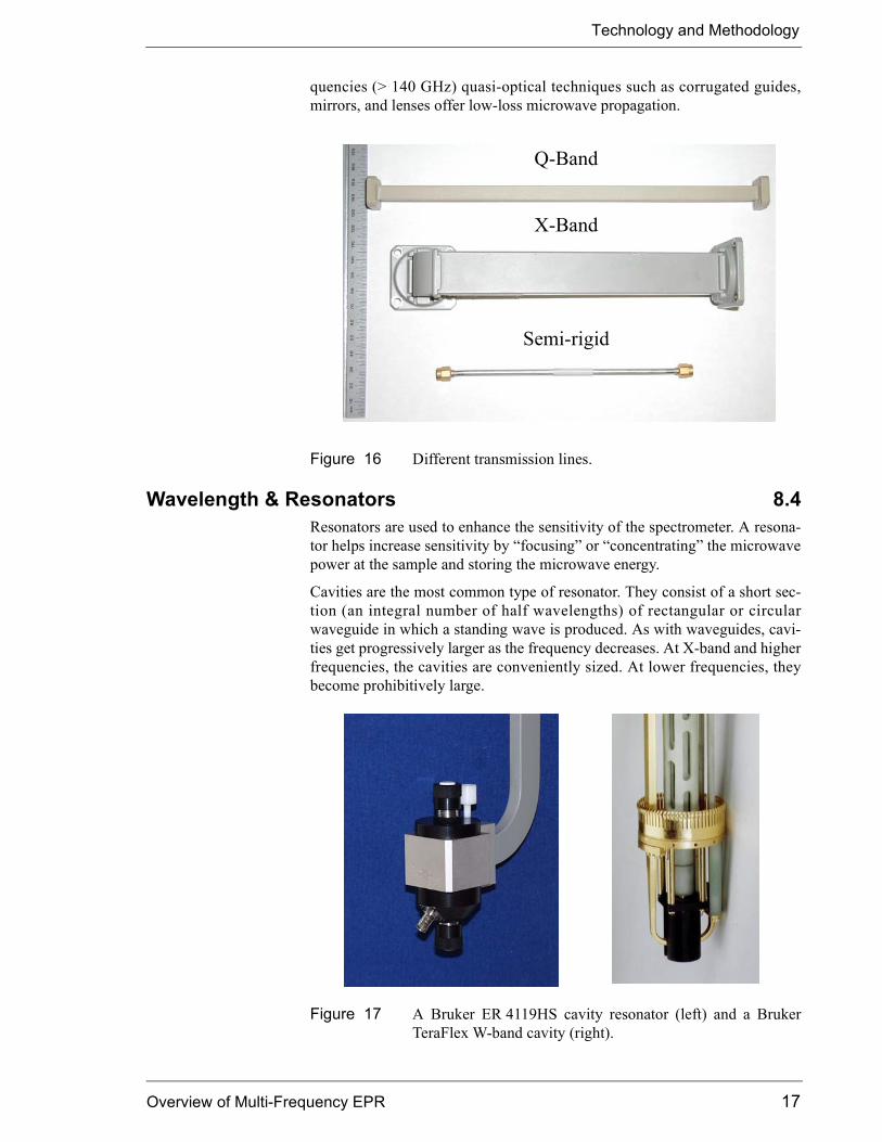
Wavelength & Resonators 8.4Resonators are used to enhance the sensitivity of the spectrometer. A resona-tor helps increase sensitivity by “focusing” or “concentrating” the microwavepower at the sample and storing the microwave energy.

Cavities are the most common type of resonator. They consist of a short sec-tion (an integral number of half wavelengths) of rectangular or circularwaveguide in which a standing wave is produced. As with waveguides, cavi-ties get progressively larger as the frequency decreases. At X-band and higherfrequencies, the cavities are conveniently sized. At lower frequencies, theybecome prohibitively large.

Figure 16 Different transmission lines.

Q-Band

X-Band

Semi-rigid

Figure 17 A Bruker ER 4119HS cavity resonator (left) and a BrukerTeraFlex W-band cavity (right).


18

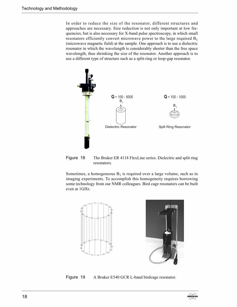
In order to reduce the size of the resonator, different structures andapproaches are necessary. Size reduction is not only important at low fre-quencies, but is also necessary for X-band pulse spectroscopy, in which smallresonators efficiently convert microwave power to the large required B1(microwave magnetic field) at the sample. One approach is to use a dielectricresonator in which the wavelength is considerably shorter than the free spacewavelength, thus shrinking the size of the resonator. Another approach is touse a different type of structure such as a split-ring or loop-gap resonator.

Sometimes, a homogeneous B1 is required over a large volume, such as inimaging experiments. To accomplish this homogeneity requires borrowingsome technology from our NMR colleagues. Bird cage resonators can be builteven at 1GHz.

Figure 18 The Bruker ER 4118 FlexLine series. Dielectric and split ringresonators.

Figure 19 A Bruker E540 GCR L-band birdcage resonator.

Split Ring ResonatorDielectric Resonator

B1

B1

Q = 100 - 5000 Q = 100 - 1000