Embed Size (px)
Citation preview

OVERFLOW 2 Training ClassAfternoon Session
Pieter G. BuningNASA Langley Research Center
Robert H. Nichols
9/20/20101
Robert H. NicholsUniversity of Alabama at BirminghamCREATE-AV API Principal Developer
10th Symposium on Overset Composite Grids& Solution Technology
NASA Ames Research CenterSeptember 20-23, 2010
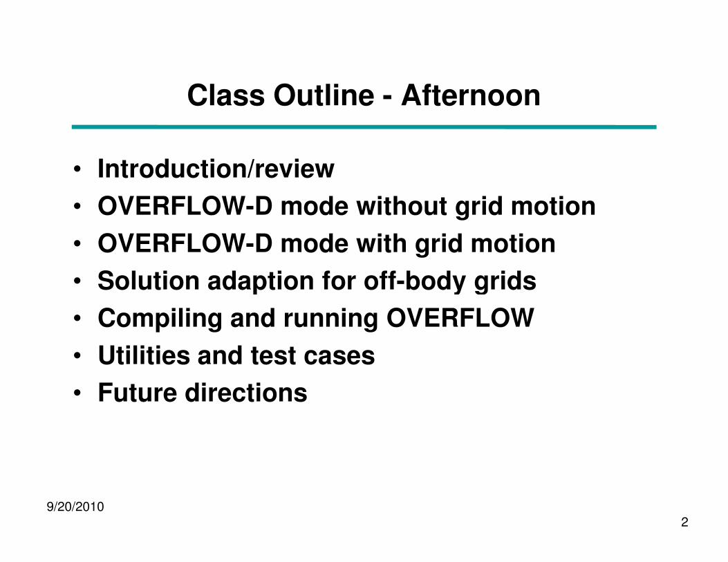
Class Outline - Afternoon
• Introduction/review
• OVERFLOW-D mode without grid motion
• OVERFLOW-D mode with grid motion
• Solution adaption for off-body grids
9/20/20102
• Solution adaption for off-body grids
• Compiling and running OVERFLOW
• Utilities and test cases
• Future directions
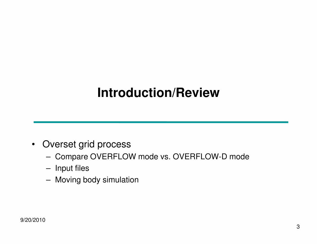
Introduction/Review
9/20/20103
• Overset grid process
– Compare OVERFLOW mode vs. OVERFLOW-D mode
– Input files
– Moving body simulation

Overset Grid Approaches
• OVERFLOW 2: two modes of operation
– OVERFLOW mode with grid joining input from Pegasus 5 or SUGGAR
– OVERFLOW-D mode using DCF
• OVERFLOW mode
– All grids are created external to the flow solver (grid.in)
– Pegasus 5 (or SUGGAR) used to cut holes and establish interpolation stencils (XINTOUT)
9/20/2010 4
(XINTOUT)
– No moving body capability
– OVERFLOW namelist input
• OVERFLOW-D mode using DCF (Domain Connectivity Function)
– Near-body grids are created external to the flow solver (grid.in)
– X-rays of body surfaces used for cutting holes (xrays.in)
– Additional namelist inputs
– Optional Geometry Manipulation Protocol (GMP) files to describe bodies and motion (Config.xml, Scenario.xml)
• OVERFLOW 2 can do either approach
– Decision is based on whether additional namelists are present in input file
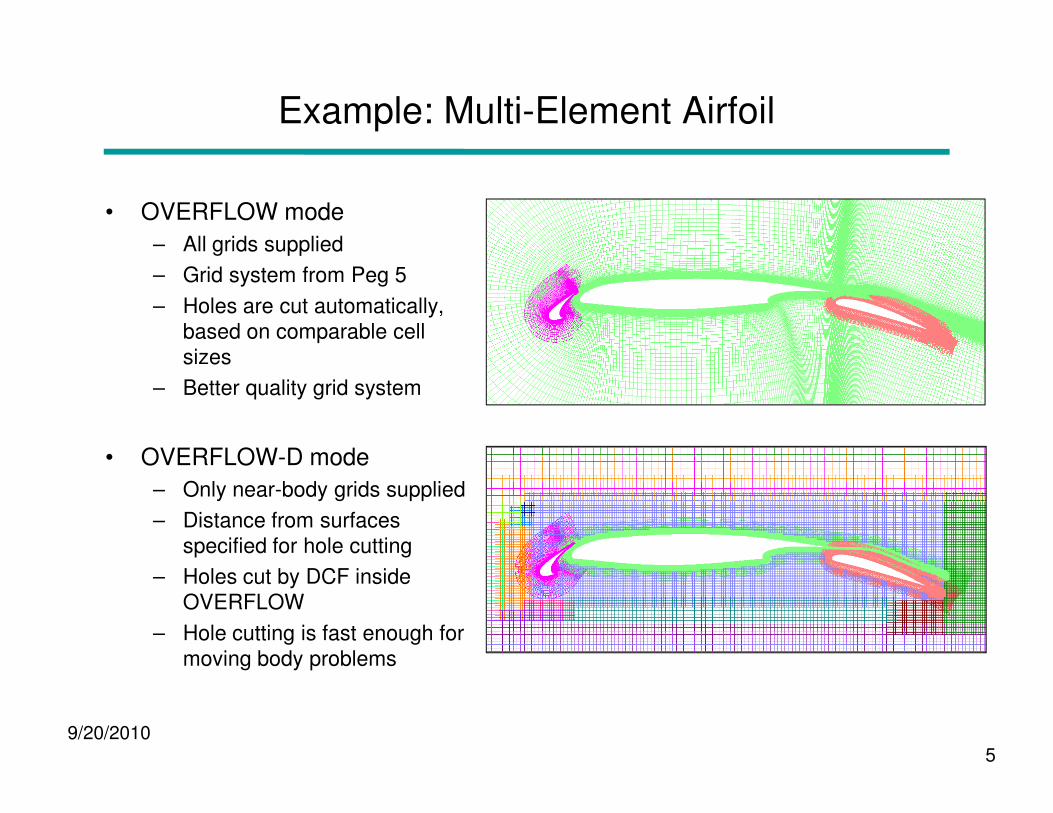
Example: Multi-Element Airfoil
• OVERFLOW mode
– All grids supplied
– Grid system from Peg 5
– Holes are cut automatically, based on comparable cell sizes
– Better quality grid system
9/20/20105
• OVERFLOW-D mode
– Only near-body grids supplied
– Distance from surfaces specified for hole cutting
– Holes cut by DCF inside OVERFLOW
– Hole cutting is fast enough for moving body problems
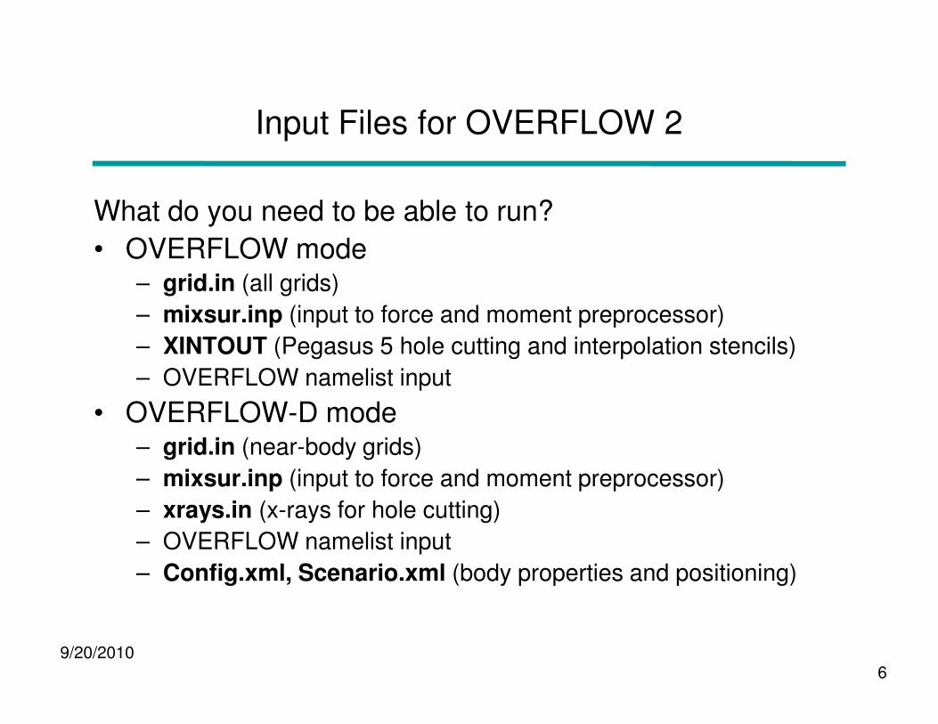
Input Files for OVERFLOW 2
What do you need to be able to run?
• OVERFLOW mode– grid.in (all grids)
– mixsur.inp (input to force and moment preprocessor)
– XINTOUT (Pegasus 5 hole cutting and interpolation stencils)
9/20/20106
– OVERFLOW namelist input
• OVERFLOW-D mode– grid.in (near-body grids)
– mixsur.inp (input to force and moment preprocessor)
– xrays.in (x-rays for hole cutting)
– OVERFLOW namelist input
– Config.xml, Scenario.xml (body properties and positioning)

Moving Body Simulation Process
• Pre-processing:
– Near-body grid generation
– Definition of force and moment integration surfaces
– Creating X-rays for hole cutting
• OVERFLOW grid processing:
– Off-body grid generation
– Hole cutting and boundary interpolation stencils
9/20/20107
– Hole cutting and boundary interpolation stencils
• Moving body simulation
– Body motion (GMP interface)
– Time-advance scheme
– Saving motion, forces, flow solution
• Post-processing
– Non-trivial!

Flow Simulation Process
• Starting and for grid adaption:
– Read near-body grids, move to dynamic position(s)
– Make off-body grids
– Interpolate flow solution onto new off-body grids
– Run DCF (cut holes, find interpolation stencils)
– Advance flow solution one step
9/20/20108
– Compute forces and moments
• Every step:
– Update near-body grid positions
– Run DCF
– Advance flow solution one step
– Compute forces and moments
OVERFLOW-D Mode Without Grid Motion
• NAMELIST inputs
9/20/2010 9
• NAMELIST inputs
• Near-body grid generation
• Force and moment integration
• Generating X-rays
• Off-body grid generation
• Grid assembly with DCF
• Data surface grids
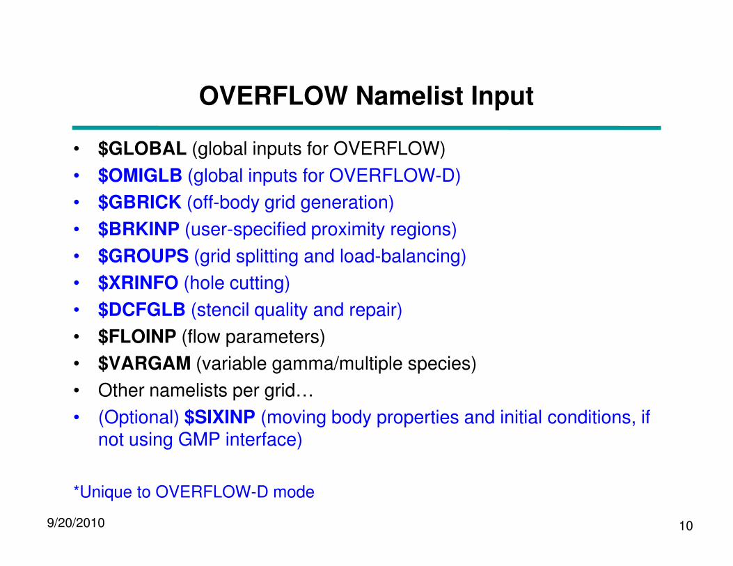
OVERFLOW Namelist Input
• $GLOBAL (global inputs for OVERFLOW)
• $OMIGLB (global inputs for OVERFLOW-D)
• $GBRICK (off-body grid generation)
• $BRKINP (user-specified proximity regions)
• $GROUPS (grid splitting and load-balancing)
• $XRINFO (hole cutting)
9/20/2010 10
• $XRINFO (hole cutting)
• $DCFGLB (stencil quality and repair)
• $FLOINP (flow parameters)
• $VARGAM (variable gamma/multiple species)
• Other namelists per grid…
• (Optional) $SIXINP (moving body properties and initial conditions, if not using GMP interface)
*Unique to OVERFLOW-D mode
OVERFLOW Namelists per Grid
• $GRDNAM (grid name)
• $NITERS (subiterations per grid)
• $METPRM (numerical method selection)
• $TIMACU (time accuracy)
• $SMOACU (smoothing parameters)
• $VISINP (viscous and turbulence modeling)
9/20/201011
• $VISINP (viscous and turbulence modeling)
• $BCINP (boundary conditions)
• $SCEINP (species convection equations)
See over2.2x/doc/namelist.pdf for a detailed list of all input parameters and definitions
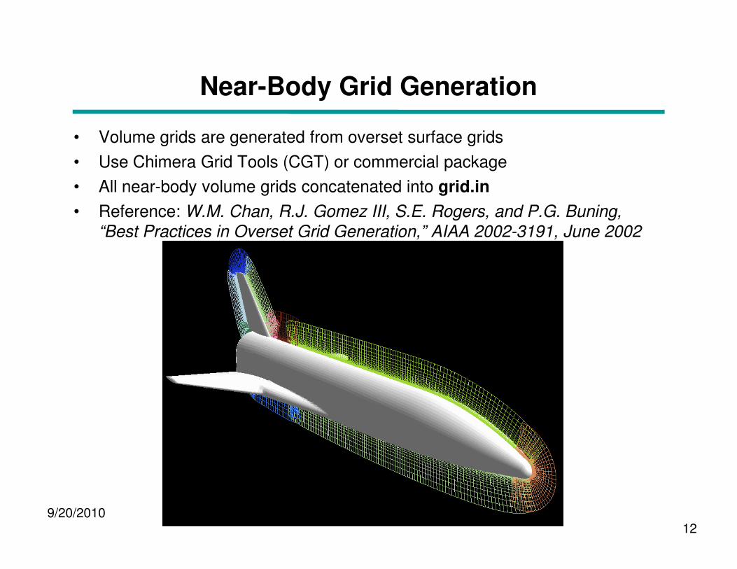
Near-Body Grid Generation
• Volume grids are generated from overset surface grids
• Use Chimera Grid Tools (CGT) or commercial package
• All near-body volume grids concatenated into grid.in
• Reference: W.M. Chan, R.J. Gomez III, S.E. Rogers, and P.G. Buning,
“Best Practices in Overset Grid Generation,” AIAA 2002-3191, June 2002
9/20/201012
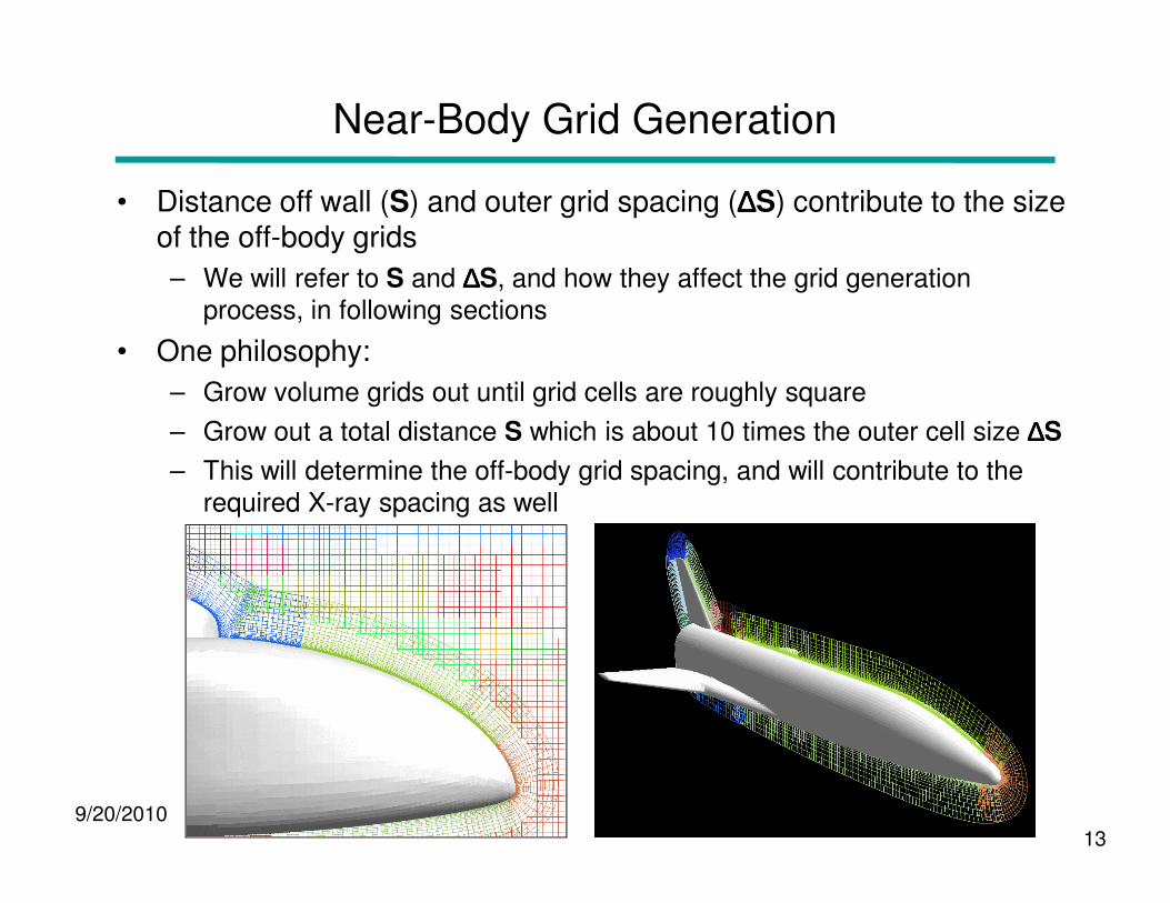
Near-Body Grid Generation
• Distance off wall (S) and outer grid spacing (∆∆∆∆S) contribute to the size of the off-body grids
– We will refer to S and ∆∆∆∆S, and how they affect the grid generation process, in following sections
• One philosophy:
– Grow volume grids out until grid cells are roughly square
– Grow out a total distance S which is about 10 times the outer cell size ∆∆∆∆S
9/20/201013
– This will determine the off-body grid spacing, and will contribute to the required X-ray spacing as well
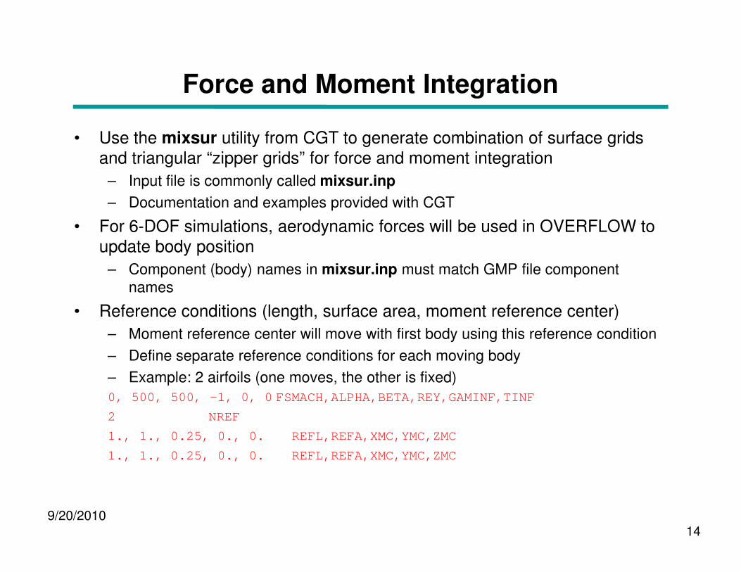
Force and Moment Integration
• Use the mixsur utility from CGT to generate combination of surface grids and triangular “zipper grids” for force and moment integration
– Input file is commonly called mixsur.inp
– Documentation and examples provided with CGT
• For 6-DOF simulations, aerodynamic forces will be used in OVERFLOW to update body position
– Component (body) names in mixsur.inp must match GMP file component names
9/20/201014
names
• Reference conditions (length, surface area, moment reference center)
– Moment reference center will move with first body using this reference condition
– Define separate reference conditions for each moving body
– Example: 2 airfoils (one moves, the other is fixed)
0, 500, 500, -1, 0, 0 FSMACH,ALPHA,BETA,REY,GAMINF,T INF
2 NREF
1., 1., 0.25, 0., 0. REFL,REFA,XMC,YMC,ZMC
1., 1., 0.25, 0., 0. REFL,REFA,XMC,YMC,ZMC

Force and Moment Integration
• For mixsur, be sure to visually check resulting integration surfaces!
– PLOT3D command files generated automatically
– Look for missing triangles, tangled zipper grids
• USURP (Unique Surfaces Using Ranked Polygons) by David Boger
9/20/201015
Ranked Polygons) by David Boger (Penn State) is an open source alternative to mixsur
– Same input file; output also recognized by OVERFLOW
– Designed to overcome zipper grid problems

Creating X-Rays
• Creating X-rays
• Picking X-ray spacing
• Using OVERGRID to create X-rays
• X-ray number and Body ID
• Using gen_x to create X-rays
9/20/201016
• Examples
• Notes and comments
Creating X-Rays
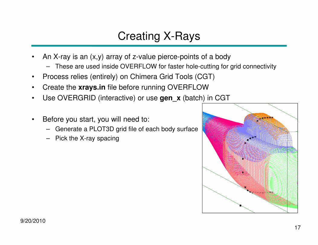
• An X-ray is an (x,y) array of z-value pierce-points of a body
– These are used inside OVERFLOW for faster hole-cutting for grid connectivity
• Process relies (entirely) on Chimera Grid Tools (CGT)
• Create the xrays.in file before running OVERFLOW
• Use OVERGRID (interactive) or use gen_x (batch) in CGT
• Before you start, you will need to:
9/20/201017
• Before you start, you will need to:
– Generate a PLOT3D grid file of each body surface
– Pick the X-ray spacing
Picking X-Ray Spacing
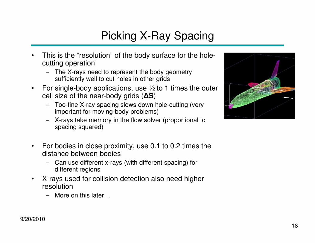
• This is the “resolution” of the body surface for the hole-cutting operation
– The X-rays need to represent the body geometry sufficiently well to cut holes in other grids
• For single-body applications, use ½ to 1 times the outer cell size of the near-body grids (∆S)
– Too-fine X-ray spacing slows down hole-cutting (very important for moving-body problems)
– X-rays take memory in the flow solver (proportional to
9/20/201018
– X-rays take memory in the flow solver (proportional to spacing squared)
• For bodies in close proximity, use 0.1 to 0.2 times the distance between bodies
– Can use different x-rays (with different spacing) for different regions
• X-rays used for collision detection also need higher resolution
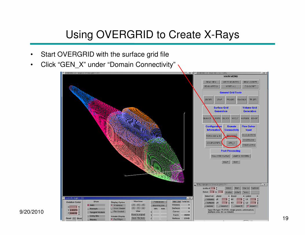
Using OVERGRID to Create X-Rays
• Start OVERGRID with the surface grid file
• Click “GEN_X” under “Domain Connectivity”
9/20/201019
Using OVERGRID to Create X-Rays
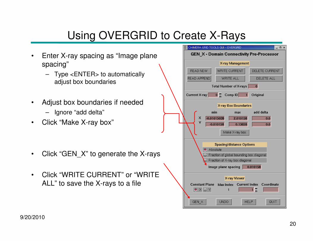
• Enter X-ray spacing as “Image plane spacing”
– Type <ENTER> to automatically adjust box boundaries
• Adjust box boundaries if needed
– Ignore “add delta”
• Click “Make X-ray box”
9/20/201020
• Click “Make X-ray box”
• Click “GEN_X” to generate the X-rays
• Click “WRITE CURRENT” or “WRITE ALL” to save the X-rays to a file
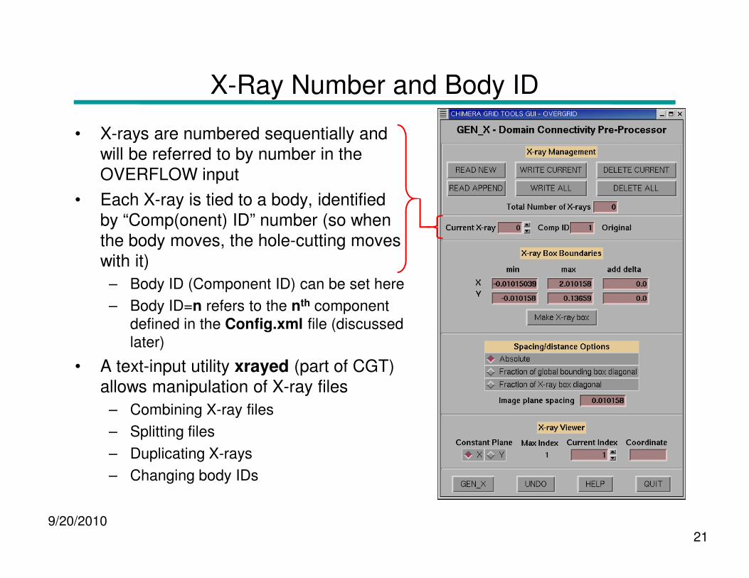
X-Ray Number and Body ID
• X-rays are numbered sequentially and will be referred to by number in the OVERFLOW input
• Each X-ray is tied to a body, identified by “Comp(onent) ID” number (so when the body moves, the hole-cutting moves with it)
– Body ID (Component ID) can be set here
9/20/201021
– Body ID (Component ID) can be set here
– Body ID=n refers to the nth component defined in the Config.xml file (discussed later)
• A text-input utility xrayed (part of CGT) allows manipulation of X-ray files
– Combining X-ray files
– Splitting files
– Duplicating X-rays
– Changing body IDs
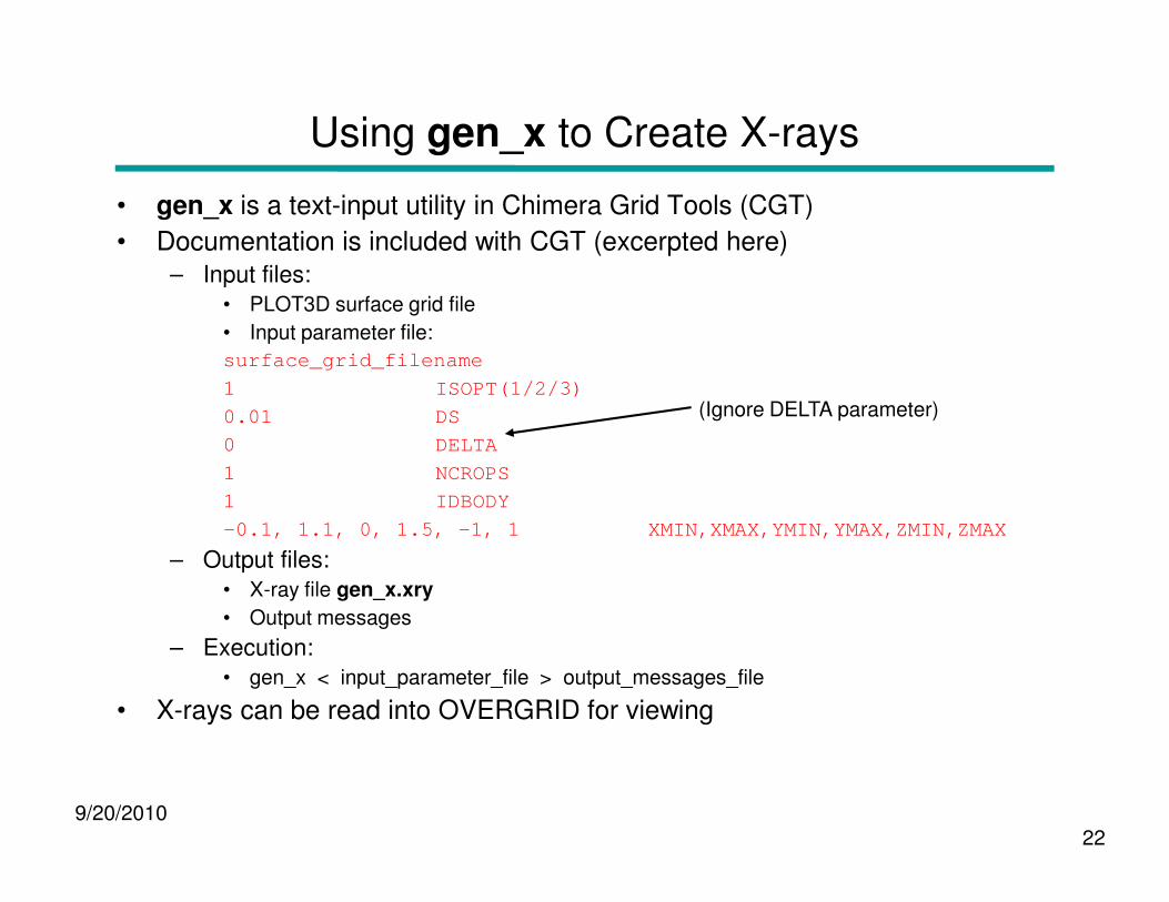
Using gen_x to Create X-rays
• gen_x is a text-input utility in Chimera Grid Tools (CGT)
• Documentation is included with CGT (excerpted here)– Input files:
• PLOT3D surface grid file
• Input parameter file:
surface_grid_filename
1 ISOPT(1/2/3)
0.01 DS
0 DELTA
(Ignore DELTA parameter)
9/20/201022
0 DELTA
1 NCROPS
1 IDBODY
-0.1, 1.1, 0, 1.5, -1, 1 XMIN,XMAX,YMIN,YMAX,ZMIN,ZM AX
– Output files:• X-ray file gen_x.xry
• Output messages
– Execution:• gen_x < input_parameter_file > output_messages_file
• X-rays can be read into OVERGRID for viewing

Example: Axisymmetric External Tank
• For 2D or axisymmetric geometries, X-rays only need to bound the center (y=0) grid plane
– Create the surface grid to represent the geometry within ± the X-ray spacing of y=0
– Set the X-ray bounding box y limits to ± the X-ray spacing
– Comparable gen_x input:
et.srf
1 ISOPT(1/2/3)
10 DS
9/20/201023
10 DS
0 DELTA
1 NCROPS
1 IDBODY
320,2180,-10,10,-200,200
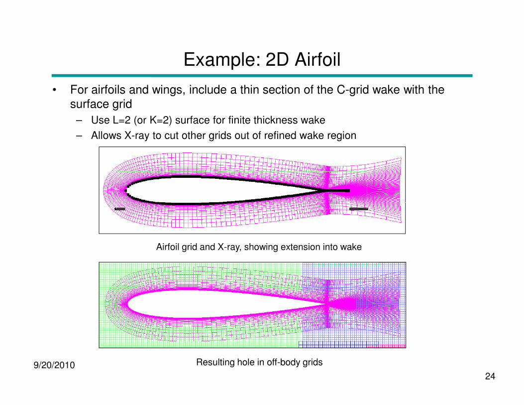
Example: 2D Airfoil
• For airfoils and wings, include a thin section of the C-grid wake with the surface grid
– Use L=2 (or K=2) surface for finite thickness wake
– Allows X-ray to cut other grids out of refined wake region
9/20/201024
Airfoil grid and X-ray, showing extension into wake
Resulting hole in off-body grids
Notes and Comments
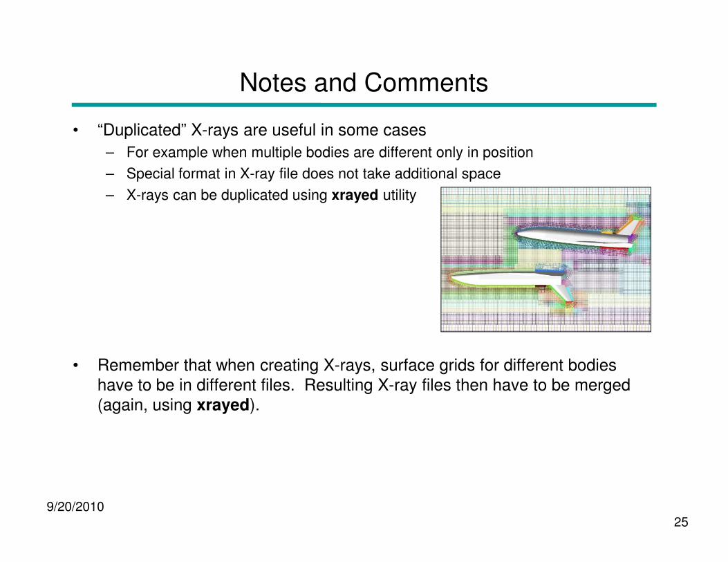
• “Duplicated” X-rays are useful in some cases
– For example when multiple bodies are different only in position
– Special format in X-ray file does not take additional space
– X-rays can be duplicated using xrayed utility
9/20/201025
• Remember that when creating X-rays, surface grids for different bodies have to be in different files. Resulting X-ray files then have to be merged (again, using xrayed).
Notes and Comments
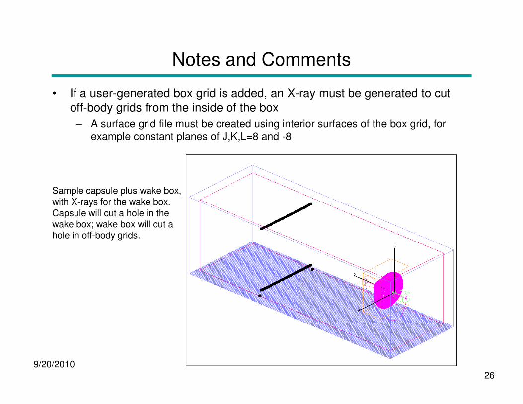
• If a user-generated box grid is added, an X-ray must be generated to cut off-body grids from the inside of the box
– A surface grid file must be created using interior surfaces of the box grid, for example constant planes of J,K,L=8 and -8
Sample capsule plus wake box, with X-rays for the wake box.
9/20/201026
with X-rays for the wake box. Capsule will cut a hole in the wake box; wake box will cut a hole in off-body grids.

Automatic Off-Body Grid Generation
• Function of off-body grids
• Basic controls
• Matching near-body and off-body grid spacing
• Specifying additional refined regions
• Controlling the rate of grid coarsening
9/20/201027
• Specifying symmetry planes, ground planes, etc.
• Far-field boundary conditions
• Examples
• Notes and comments
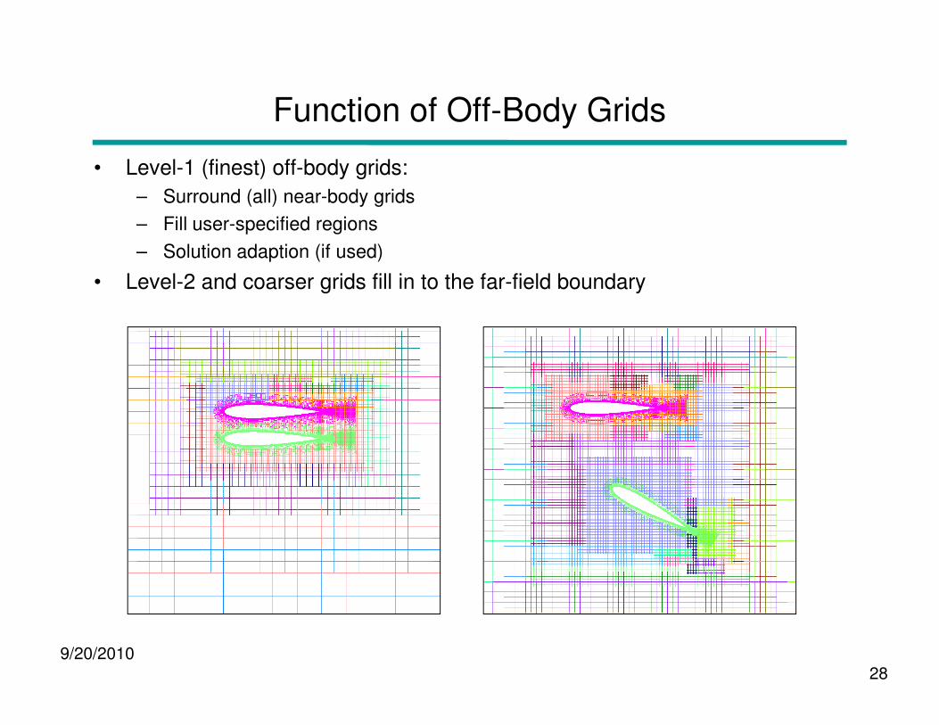
Function of Off-Body Grids
• Level-1 (finest) off-body grids:
– Surround (all) near-body grids
– Fill user-specified regions
– Solution adaption (if used)
• Level-2 and coarser grids fill in to the far-field boundary
9/20/201028
Basic Controls
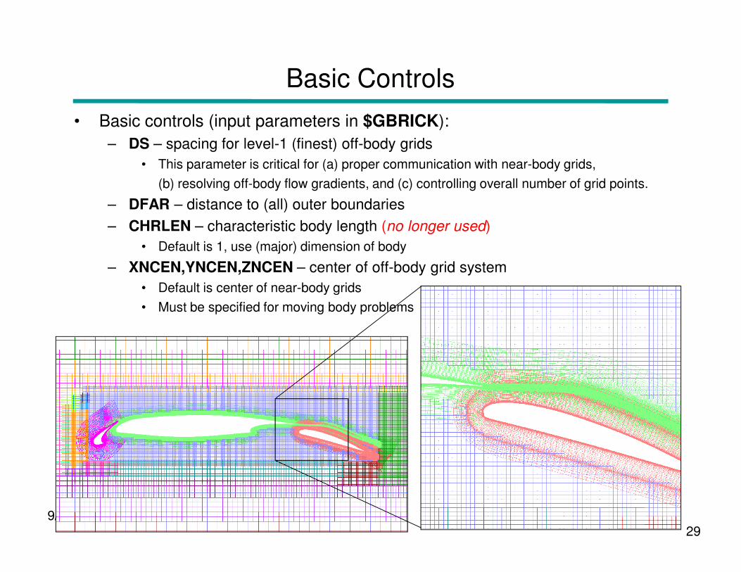
• Basic controls (input parameters in $GBRICK):
– DS – spacing for level-1 (finest) off-body grids
• This parameter is critical for (a) proper communication with near-body grids,
(b) resolving off-body flow gradients, and (c) controlling overall number of grid points.
– DFAR – distance to (all) outer boundaries
– CHRLEN – characteristic body length (no longer used)
• Default is 1, use (major) dimension of body
– XNCEN,YNCEN,ZNCEN – center of off-body grid system
• Default is center of near-body grids
9/20/201029
• Default is center of near-body grids
• Must be specified for moving body problems
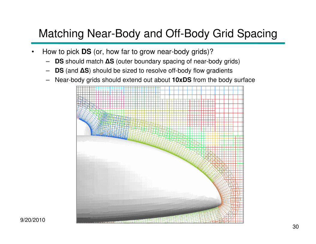
Matching Near-Body and Off-Body Grid Spacing
• How to pick DS (or, how far to grow near-body grids)?
– DS should match ∆S (outer boundary spacing of near-body grids)
– DS (and ∆S) should be sized to resolve off-body flow gradients
– Near-body grids should extend out about 10xDS from the body surface
9/20/201030
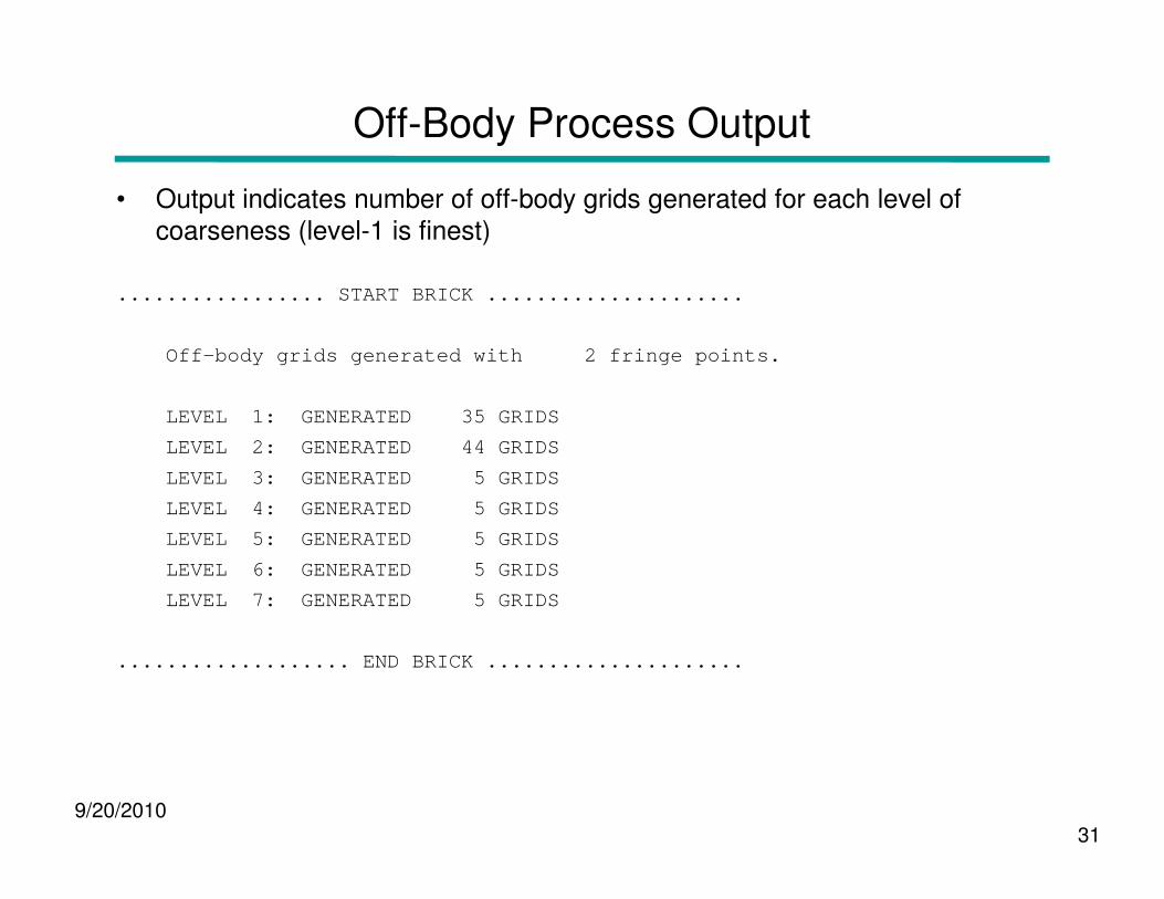
Off-Body Process Output
• Output indicates number of off-body grids generated for each level of coarseness (level-1 is finest)
................. START BRICK .....................
Off-body grids generated with 2 fringe points.
LEVEL 1: GENERATED 35 GRIDS
LEVEL 2: GENERATED 44 GRIDS
9/20/201031
LEVEL 2: GENERATED 44 GRIDS
LEVEL 3: GENERATED 5 GRIDS
LEVEL 4: GENERATED 5 GRIDS
LEVEL 5: GENERATED 5 GRIDS
LEVEL 6: GENERATED 5 GRIDS
LEVEL 7: GENERATED 5 GRIDS
................... END BRICK .....................
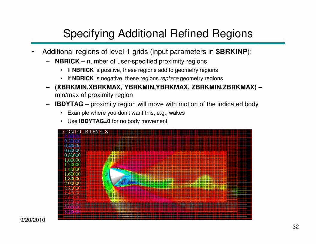
Specifying Additional Refined Regions
• Additional regions of level-1 grids (input parameters in $BRKINP):
– NBRICK – number of user-specified proximity regions
• If NBRICK is positive, these regions add to geometry regions
• If NBRICK is negative, these regions replace geometry regions
– (XBRKMIN,XBRKMAX, YBRKMIN,YBRKMAX, ZBRKMIN,ZBRKMAX) –min/max of proximity region
– IBDYTAG – proximity region will move with motion of the indicated body
• Example where you don’t want this, e.g., wakes
• Use IBDYTAG=0 for no body movement
9/20/201032
• Use IBDYTAG=0 for no body movement

Controlling the Rate of Grid Coarsening
• Effect of MINBUF (in $GBRICK):
– Default MINBUF=4 gives minimum overlap between successively coarser off-body grids
– Larger values give more gradual coarsening, but use more grid points
– 2-airfoil example:
• MINBUF=4 (if geometry were 3D, off-body grids would have 2 million points)
• MINBUF=8 (3D off-body grids would have 3 million points)
9/20/201033
MINBUF=4 MINBUF=8

Specifying Symmetry Planes, Ground Planes, etc.
• Special planes (input parameters in $GBRICK):
– Used to set a ground plane, symmetry plane, inflow plane, etc.
– I_XMIN=1 – use value of P_XMIN as off-body grid X(minimum)
– I_XMIN=0 – default is to use DFAR to set X (minimum)
– Same for I_XMAX, I_YMIN,I_YMAX, I_ZMIN,I_ZMAX, and P_XMAX, P_YMIN,P_YMAX, P_ZMIN,P_ZMAX
– Can only set one out of each (x,y,z) pair of values
9/20/2010 34
Symmetry plane for helicopter fuselage:I_YMIN=1, P_YMIN=0
Hyper-X supersonic inflow plane:I_XMIN=1, P_XMIN=-20
Far-Field Boundary Conditions
• Far-field boundary conditions (input parameters in $OMIGLB):
– IBXMIN – boundary condition type for off-body grid system X (minimum) boundary
– Same for IBXMAX, IBYMIN,IBYMAX, IBZMIN,IBZMAX
– A limited number of boundary conditions are implemented:
• Inflow/outflow conditions: BC types 30,35,37,40,41,47,49
• 2D or axisymmetric condition (y only): BC types 21,22
• Axis condition (z only, and combined with axisymmetric in y): BC type 16
• Symmetry conditions: BC types 11,12,13,17
9/20/201035
• Symmetry conditions: BC types 11,12,13,17
• Inviscid wall: BC type 1
– Default is free-stream/characteristic condition (BC type 47)
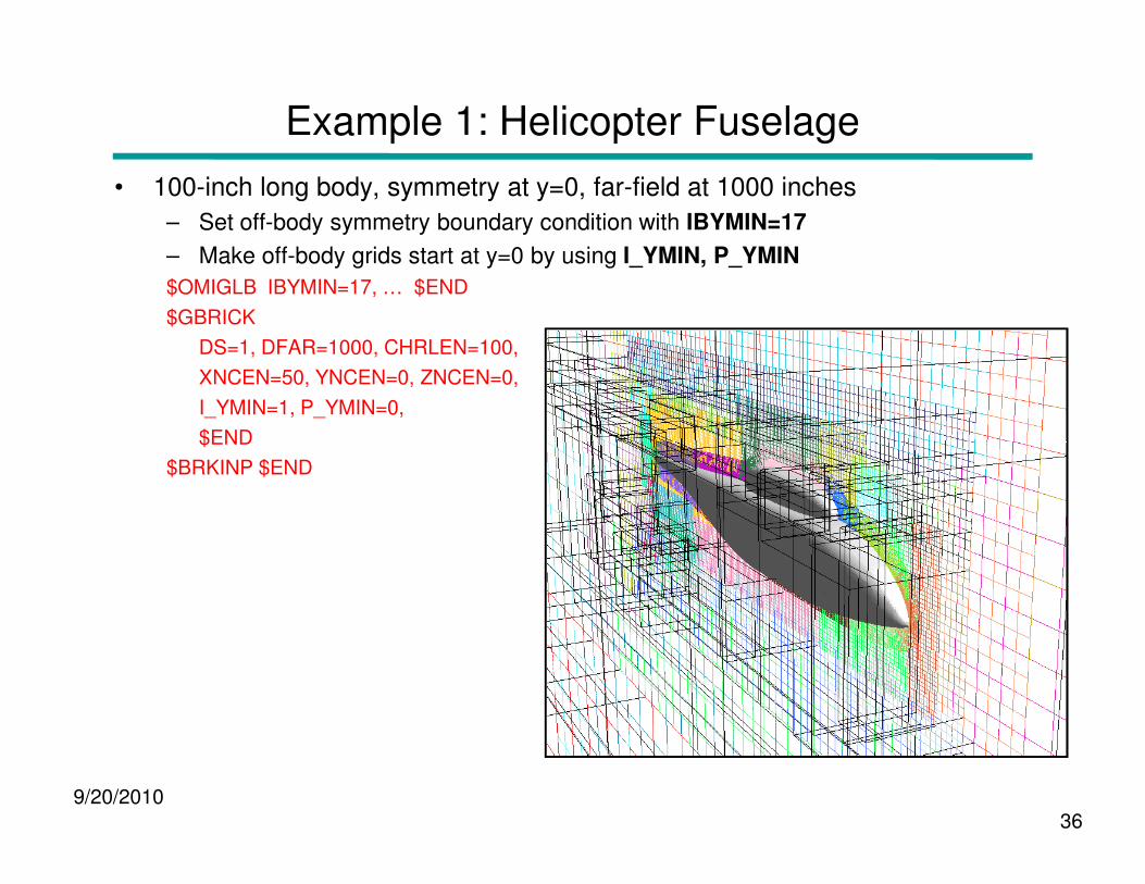
Example 1: Helicopter Fuselage
• 100-inch long body, symmetry at y=0, far-field at 1000 inches
– Set off-body symmetry boundary condition with IBYMIN=17
– Make off-body grids start at y=0 by using I_YMIN, P_YMIN
$OMIGLB IBYMIN=17, … $END
$GBRICK
DS=1, DFAR=1000, CHRLEN=100,
XNCEN=50, YNCEN=0, ZNCEN=0,
I_YMIN=1, P_YMIN=0,
$END
9/20/201036
$END
$BRKINP $END
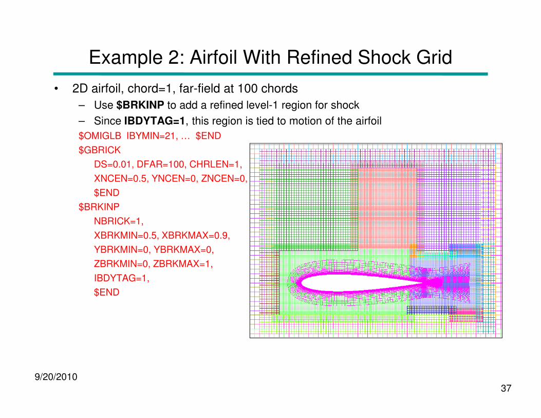
Example 2: Airfoil With Refined Shock Grid
• 2D airfoil, chord=1, far-field at 100 chords
– Use $BRKINP to add a refined level-1 region for shock
– Since IBDYTAG=1, this region is tied to motion of the airfoil
$OMIGLB IBYMIN=21, … $END
$GBRICK
DS=0.01, DFAR=100, CHRLEN=1,
XNCEN=0.5, YNCEN=0, ZNCEN=0,
$END
$BRKINP
9/20/201037
$BRKINP
NBRICK=1,
XBRKMIN=0.5, XBRKMAX=0.9,
YBRKMIN=0, YBRKMAX=0,
ZBRKMIN=0, ZBRKMAX=1,
IBDYTAG=1,
$END
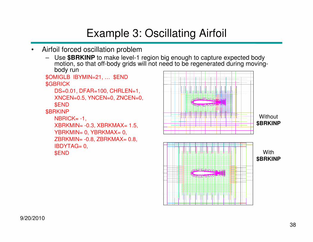
Example 3: Oscillating Airfoil
• Airfoil forced oscillation problem– Use $BRKINP to make level-1 region big enough to capture expected body
motion, so that off-body grids will not need to be regenerated during moving-body run
$OMIGLB IBYMIN=21, … $END
$GBRICK
DS=0.01, DFAR=100, CHRLEN=1,
XNCEN=0.5, YNCEN=0, ZNCEN=0,
$END
$BRKINP
NBRICK= -1, Without$BRKINP
9/20/201038
NBRICK= -1,
XBRKMIN= -0.3, XBRKMAX= 1.5,
YBRKMIN= 0, YBRKMAX= 0,
ZBRKMIN= -0.8, ZBRKMAX= 0.8,
IBDYTAG= 0,
$END
$BRKINP
With$BRKINP

Example 3: Oscillating Airfoil
• Airfoil forced oscillation problem– Use $BRKINP to make level-1 region big enough to capture expected body
motion, so that off-body grids will not need to be regenerated during moving-body run
$OMIGLB IBYMIN=21, … $END
$GBRICK
DS=0.01, DFAR=100, CHRLEN=1,
XNCEN=0.5, YNCEN=0, ZNCEN=0,
$END
$BRKINP
NBRICK= -1, Without$BRKINP
9/20/201039
NBRICK= -1,
XBRKMIN= -0.3, XBRKMAX= 1.5,
YBRKMIN= 0, YBRKMAX= 0,
ZBRKMIN= -0.8, ZBRKMAX= 0.8,
IBDYTAG= 0,
$END
$BRKINP
With$BRKINP
Notes and Comments
• OBGRIDS=FALSE – no off-body grids created
– For single-grid problems, or where background grids are already supplied
• Files created: brkset.save, brkset.restart
– Needed for moving body restarts to generate consistent off-body grids
– Delete these files to force OVERFLOW to generate new off-body grids (for example, if you change the input parameters)
• Residual history for off-body grids is grouped by level in resid.out, turb.out, species.out
9/20/201040
species.out
– Instead of one entry per level-n grid, there is one entry representing all level-n grids
– Entry contains L2 and L∞-norms of RHS and ∆Q
– Entry lists (x,y,z) instead of (j,k,l) location of L∞-norm (off-body grids only)
– Especially appropriate for moving body or solution adaption problems, where the number of off-body grids changes every adapt cycle
DCF: Hole Cutting and Grid Assembly
• Using X-rays to cut holes
• Choosing XDELTA
• Orphan points and donor quality
• Double fringe interpolation
• Viscous stencil repair
9/20/201041
• Examples
• Notes and comments
Using X-Rays to Cut Holes
• Specifying X-ray cutters (input parameters in multiple $XRINFO):
– IDXRAY – X-ray number
– IGXLIST – list of grids to be cut
• Special grid number “-1” refers to (all) off-body grids
– Or use IGXBEG,IGXEND – starting/ending grids to be cut
– XDELTA – offset of hole from body surface
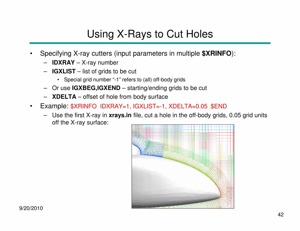
• Example: $XRINFO IDXRAY=1, IGXLIST=-1, XDELTA=0.05 $END
– Use the first X-ray in xrays.in file, cut a hole in the off-body grids, 0.05 grid units
9/20/201042
– Use the first X-ray in xrays.in file, cut a hole in the off-body grids, 0.05 grid units off the X-ray surface:

Using X-Rays to Cut Holes
• Example: multi-element airfoil$XRINFO IDXRAY=1, IGXLIST=-1, XDELTA=0.02 $END
$XRINFO IDXRAY=2, IGXLIST=-1, XDELTA=0.02 $END
$XRINFO IDXRAY=3, IGXLIST=-1, XDELTA=0.02 $END
– Slat, main, and flap X-rays (X-rays 1,2,3) cut holes in off-body grids
$XRINFO IDXRAY=1, IGXLIST=2, XDELTA=0.005 $END
– Slat X-ray cuts hole in main grid (grid 2)
$XRINFO IDXRAY=2, IGXLIST=1,3, XDELTA=0.005 $END
– Main X-ray cuts hole in slat and flap grids (grids 1,3)
9/20/201043
– Main X-ray cuts hole in slat and flap grids (grids 1,3)
$XRINFO IDXRAY=3, IGXLIST=2, XDELTA=0.005 $END
– Flap X-ray cuts hole in main grid (grid 2)
Choosing XDELTA
• Holes should be cut to keep coarser grids out of high-gradient regions (such as boundary layers)
• Holes should be cut so that grids have similar resolution in overlap regions, and have sufficient overlap for interpolation of boundary data
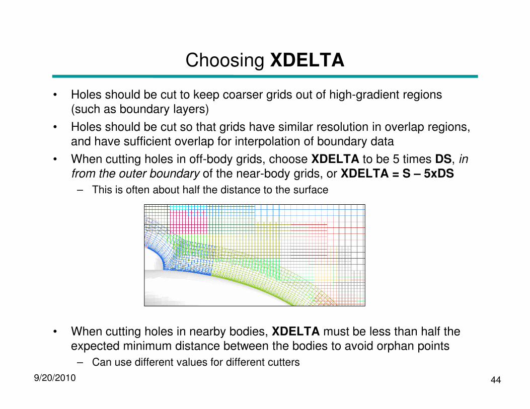
• When cutting holes in off-body grids, choose XDELTA to be 5 times DS, in
from the outer boundary of the near-body grids, or XDELTA = S – 5xDS
– This is often about half the distance to the surface
9/20/2010 44
• When cutting holes in nearby bodies, XDELTA must be less than half the expected minimum distance between the bodies to avoid orphan points
– Can use different values for different cutters

Orphan Points and Donor Quality
• Some overset grid definitions (thanks to Ralph Noack):
– Blanked-out points – points inside bodies or holes, where the solution is not computed or is ignored
– Fringe points – inter-grid boundary points where solution values are obtained via interpolation from another grid
– Donor points – points contributing to interpolation stencils
– Orphan points – fringe points without valid donors; resulting from hole cutting failure (no possible donor) or only poor quality donors are available (insufficient overlap)
9/20/2010 45
overlap)
• Donor stencil quality (input parameter in $DCFGLB):
– “Quality” of the donor stencil refers to how much of the interpolated information has to come from donor points that are interior to the flow solution, i.e., not fringe points themselves
– DQUAL=1 – donor stencils must consist of only field points (default)
– DQUAL=0 – stencils which include all fringe points may be accepted
• This is not a good idea—the simulation may simply pass boundary data back and forth between grids
– DQUAL=0.1 is generally acceptable
Double Fringe Interpolation
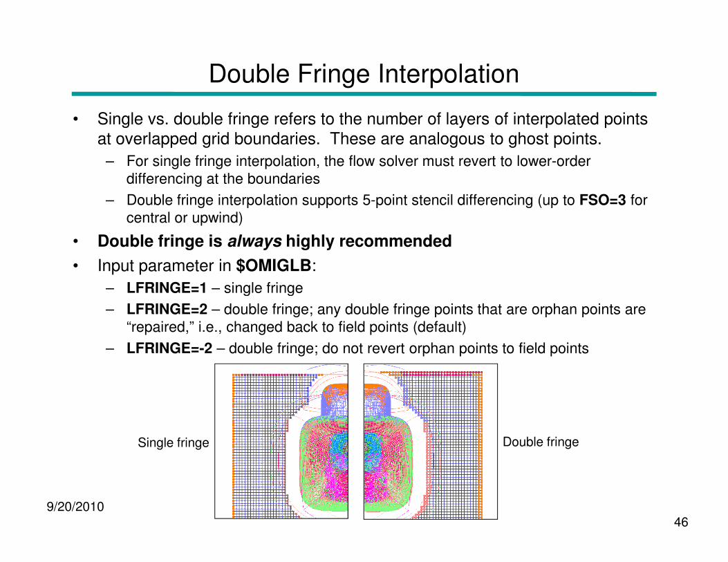
• Single vs. double fringe refers to the number of layers of interpolated points at overlapped grid boundaries. These are analogous to ghost points.
– For single fringe interpolation, the flow solver must revert to lower-order differencing at the boundaries
– Double fringe interpolation supports 5-point stencil differencing (up to FSO=3 for central or upwind)
• Double fringe is always highly recommended
• Input parameter in $OMIGLB:
– LFRINGE=1 – single fringe
9/20/201046
– LFRINGE=1 – single fringe
– LFRINGE=2 – double fringe; any double fringe points that are orphan points are “repaired,” i.e., changed back to field points (default)
– LFRINGE=-2 – double fringe; do not revert orphan points to field points
Single fringe Double fringe
Triple (and Higher) Fringe Interpolation
• Higher-order schemes in OVERFLOW need more than double fringe
– 4th-order central, 5th-order WENO schemes need LFRINGE=3
– 6th-order central needs LFRINGE=4
– Default LFRINGE is based on numerical scheme
– LFRINGE can be changed whenever grid connectivity is recomputed (DCF process)
• Off-body grids need more overlap as well
– Use OFRINGE in $GBRICK to specify number of fringe points for off-body grids
9/20/201047
– Default OFRINGE is based on numerical scheme
– But, OFRINGE cannot be changed without regenerating off-body grids
– If you plan to use a higher-order scheme later, set OFRINGE now
• Orphan points cause fringe layers to degrade gradually
– Triple fringe will locally change to double fringe, then to single fringe until orphans are resolved or converted to field points

Viscous Stencil Repair
• Viscous stencil repair (input parameters in $DCFGLB):
– MORFAN – enable/disable viscous stencil repair (1/0)
– NORFAN – number of points above a viscous wall subject to viscous stencil repair
– Viscous stencil repair is needed to handle bad interpolations when overlapping surface grids lie on the same curved surface. If not corrected, this can result in orphan points (convex surfaces) or interpolations too high in the boundary layer (concave surfaces).
– WARNING: Interpolation stencils for boundary points within NORFAN points of a
9/20/201048
– WARNING: Interpolation stencils for boundary points within NORFAN points of a viscous surface will be modified, using the assumption that all viscous walls have the same grid distribution in the normal direction. QUALITY OF REPAIRED STENCILS IS NOT CHECKED.
– A better scheme is needed!
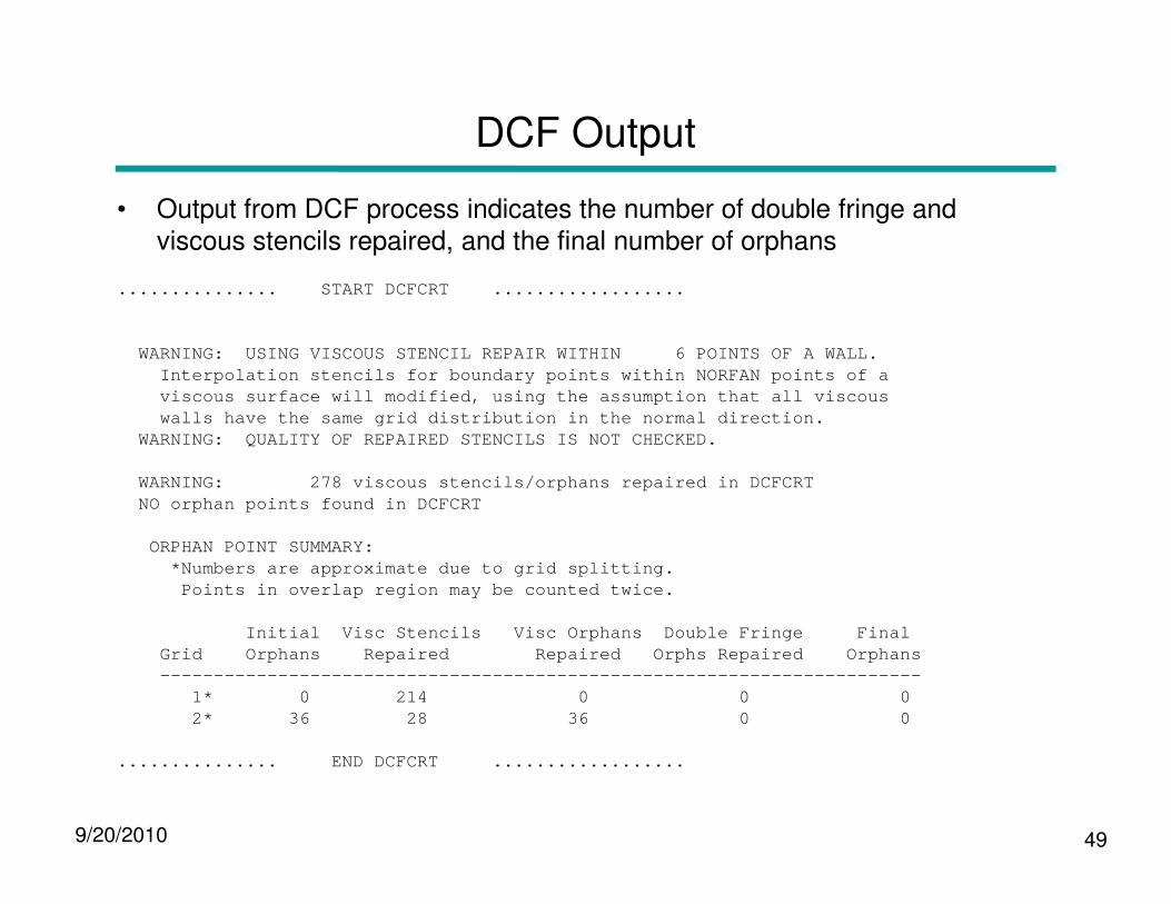
DCF Output
• Output from DCF process indicates the number of double fringe and viscous stencils repaired, and the final number of orphans
............... START DCFCRT ..................
WARNING: USING VISCOUS STENCIL REPAIR WITHIN 6 POINTS OF A WALL.Interpolation stencils for boundary points within NORFAN points of aviscous surface will modified, using the assumption that all viscouswalls have the same grid distribution in the normal direction.
WARNING: QUALITY OF REPAIRED STENCILS IS NOT CHECKED.
9/20/2010 49
WARNING: 278 viscous stencils/orphans repaired in DCFCRTNO orphan points found in DCFCRT
ORPHAN POINT SUMMARY:*Numbers are approximate due to grid splitting.
Points in overlap region may be counted twice.
Initial Visc Stencils Visc Orphans Double Fringe FinalGrid Orphans Repaired Repaired Orphs Repaired Orphans-----------------------------------------------------------------------
1* 0 214 0 0 02* 36 28 36 0 0
............... END DCFCRT ..................
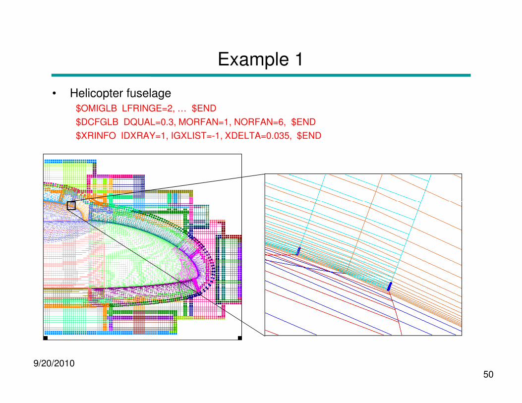
Example 1
• Helicopter fuselage$OMIGLB LFRINGE=2, … $END
$DCFGLB DQUAL=0.3, MORFAN=1, NORFAN=6, $END
$XRINFO IDXRAY=1, IGXLIST=-1, XDELTA=0.035, $END
9/20/201050

Example 2
• Airfoil drop
– For bodies that are very close to each other, very small values of XDELTA may be needed
$OMIGLB LFRINGE=2, … $END$DCFGLB DQUAL=0.3, $END$XRINFO IDXRAY=1, IGXLIST=2,-1, XDELTA=0.04, $END$XRINFO IDXRAY=2, IGXLIST=1,-1, XDELTA=0.04, $END
$OMIGLB LFRINGE=2, … $END$DCFGLB DQUAL=0.3, $END$XRINFO IDXRAY=1, IGXLIST=-1, XDELTA=0.04, $END$XRINFO IDXRAY=2, IGXLIST=-1, XDELTA=0.04, $END$XRINFO IDXRAY=1, IGXLIST=2, XDELTA=0.0, $END$XRINFO IDXRAY=2, IGXLIST=1, XDELTA=0.0, $END
9/20/2010 51
Notes and Comments
• It is OK to have “some” orphan points
– But you should understand why, and where they are in the grid system
– Be careful of compromising grid quality because you don’t want to refine the off-body grids, or don’t want to fix the near-body grids
• Orphan points become much harder to control in moving body problems
– Have to anticipate grid movement
• OVERFLOW “fills” orphan points (and all hole points) with average of neighboring point values
9/20/201052
neighboring point values
• Input parameter IRUN in $OMIGLB allows test run of DCF:
– IRUN=1 – just do off-body grid generation (write x.save file)
– IRUN=2 – do off-body grid generation and DCF (write x.save)
– IRUN=0 – do a complete run, including flow solver
– When changing inputs, be sure to delete brkset.restart and INTOUT, or OVERFLOW will not rerun these steps
Data Surface Grids
• Can be used to extract acoustic data surfaces, velocity profiles, pressure tap locations, 2D slices, etc.
• Any “1D” or “2D” (mx1x1 or mxnx1) grid in the grid.in file will be treated by DCF as a “data surface grid”
– Flow solution at all points will be interpolated from other grids
– Grid and solution will be saved in usual files (x.save, q.save)
– Can also write these out explicitly using $SPLITM
9/20/201053
OVERFLOW-D Mode With Grid Motion
• General moving body process
9/20/2010 54
• General moving body process
• Off-body grid adaption to geometry
• GMP files Config.xml and Scenario.xml
• Non-dimensionalization of dynamics quantities
• Time step specification
• Simulating collisions
• Output information for moving body problems
• Visualizing body motion in OVERGRID
• Some references
General Moving Body Process
• Current recommendation: run OVERFLOW in double precision
– Quaternion variables need to be stored as 64-bit (most, but not all complete)
• General process (input parameters in $OMIGLB):
– DYNMCS=.TRUE. – enable body dynamics (default is FALSE)
– I6DOF=2 – Prescribed and/or 6-DOF motion for different components. Specified via the GMP interface (Config.xml and Scenario.xml files) ($SIXINPis ignored). This is the recommended (and supported) option for moving body problems.
9/20/201055
• I6DOF=1 – 6-DOF body motion, specified via $SIXINP namelist input.
• I6DOF=0 – User-specified motion, controlled by user-supplied USER6 subroutine.
– NADAPT – number of steps between adaption (regeneration) of the off-body grid system
• NADAPT=-n – off-body grids adapt to geometry only
• NADAPT=0 – off-body grids will not be regenerated during solution process
• NADAPT=n – off-body grids adapt to geometry and flow solution (see next section)
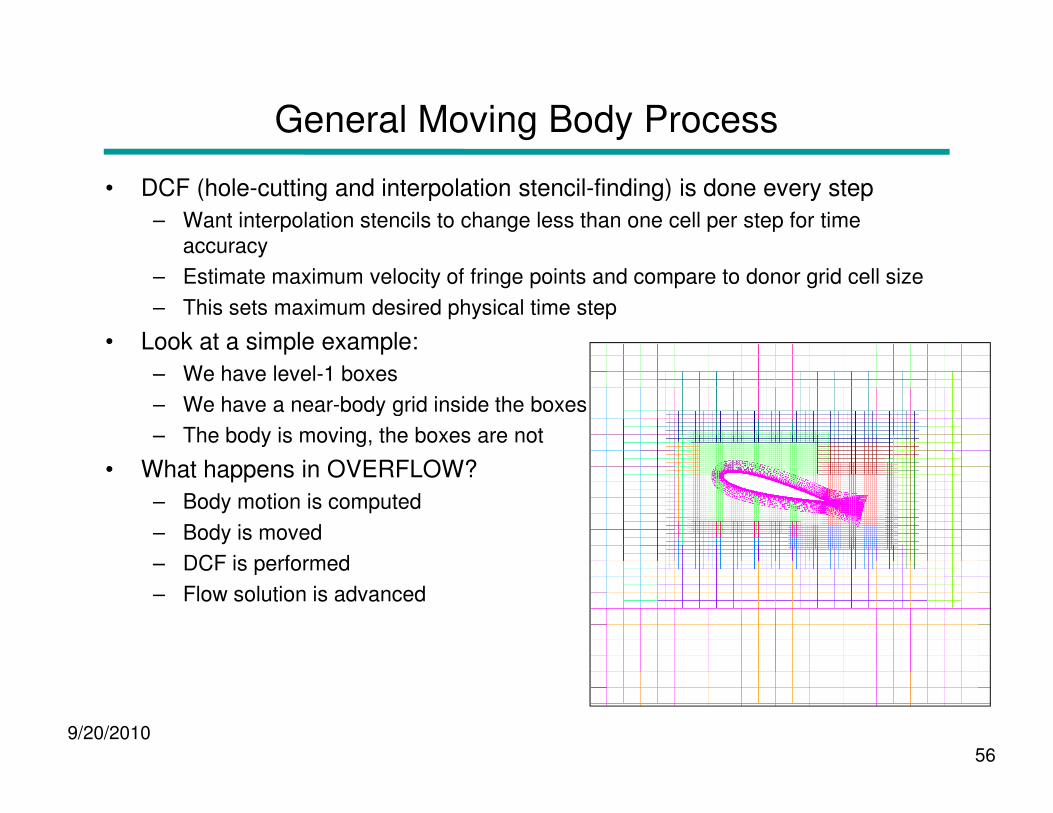
General Moving Body Process
• DCF (hole-cutting and interpolation stencil-finding) is done every step
– Want interpolation stencils to change less than one cell per step for time accuracy
– Estimate maximum velocity of fringe points and compare to donor grid cell size
– This sets maximum desired physical time step
• Look at a simple example:
– We have level-1 boxes
– We have a near-body grid inside the boxes
9/20/201056
– We have a near-body grid inside the boxes
– The body is moving, the boxes are not
• What happens in OVERFLOW?
– Body motion is computed
– Body is moved
– DCF is performed
– Flow solution is advanced
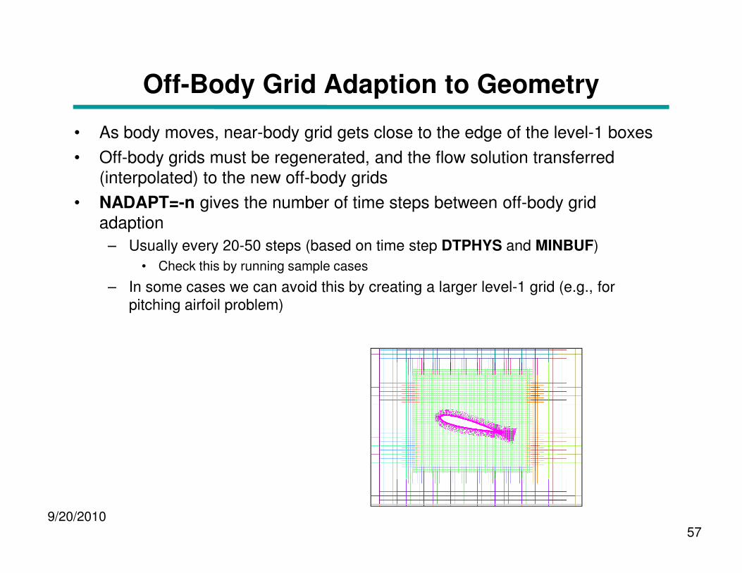
Off-Body Grid Adaption to Geometry
• As body moves, near-body grid gets close to the edge of the level-1 boxes
• Off-body grids must be regenerated, and the flow solution transferred (interpolated) to the new off-body grids
• NADAPT=-n gives the number of time steps between off-body grid adaption
– Usually every 20-50 steps (based on time step DTPHYS and MINBUF)
• Check this by running sample cases
– In some cases we can avoid this by creating a larger level-1 grid (e.g., for
9/20/201057
– In some cases we can avoid this by creating a larger level-1 grid (e.g., for pitching airfoil problem)
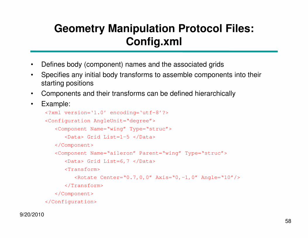
Geometry Manipulation Protocol Files: Config.xml
• Defines body (component) names and the associated grids
• Specifies any initial body transforms to assemble components into their starting positions
• Components and their transforms can be defined hierarchically
• Example:<?xml version=‘1.0’ encoding=‘utf-8’?>
<Configuration AngleUnit=“degree”>
9/20/201058
<Configuration AngleUnit=“degree”>
<Component Name=“wing” Type=“struc”>
<Data> Grid List=1-5 </Data>
</Component>
<Component Name=“aileron” Parent=“wing” Type=“struc ”>
<Data> Grid List=6,7 </Data>
<Transform>
<Rotate Center=“0.7,0,0” Axis=“0,-1,0” Angle=“10”/>
</Transform>
</Component>
</Configuration>
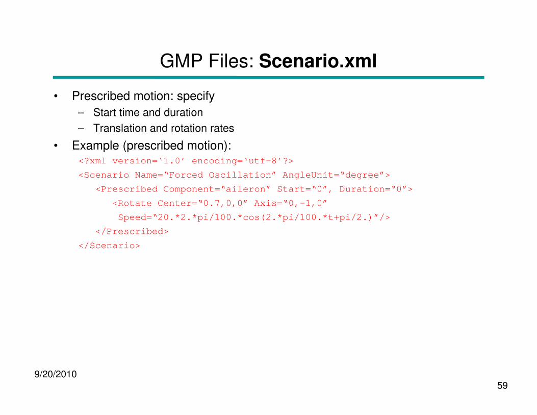
GMP Files: Scenario.xml
• Prescribed motion: specify
– Start time and duration
– Translation and rotation rates
• Example (prescribed motion):<?xml version=‘1.0’ encoding=‘utf-8’?>
<Scenario Name=“Forced Oscillation” AngleUnit=“degr ee”>
<Prescribed Component=“aileron” Start=“0”, Duration =“0”>
<Rotate Center=“0.7,0,0” Axis=“0, - 1,0”
9/20/201059
<Rotate Center=“0.7,0,0” Axis=“0, - 1,0”
Speed=“20.*2.*pi/100.*cos(2.*pi/100.*t+pi/2.)”/>
</Prescribed>
</Scenario>

GMP Files: Scenario.xml
• 6-DOF motion: specify
– Start time and duration
– Component inertial properties
– Applied forces
– Motion constraints
• Example (constrained 6-DOF motion):<?xml version=‘1.0’ encoding=‘utf-8’?>
<Scenario Name=“Constrained Motion” AngleUnit=“degr ee”>
9/20/201060
<Scenario Name=“Constrained Motion” AngleUnit=“degr ee”>
<Aero6dof Component=“aileron” Start=“0”, Duration=“ 0”>
<InertialProperties Mass=“1.0” CenterOfMass=“0.7,0, 0”
PrincipalMomentsOfInertia=“0,2,0”/>
<Constraint Rotate=“1,0,1” Frame=“body” Start=“0”/>
<Constraint Translate=“1,1,1” Frame=“body” Start=“0 ”/>
</Aero6dof>
</Scenario>
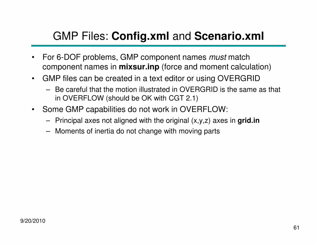
GMP Files: Config.xml and Scenario.xml
• For 6-DOF problems, GMP component names must match component names in mixsur.inp (force and moment calculation)
• GMP files can be created in a text editor or using OVERGRID
– Be careful that the motion illustrated in OVERGRID is the same as that in OVERFLOW (should be OK with CGT 2.1)
• Some GMP capabilities do not work in OVERFLOW:
– Principal axes not aligned with the original (x,y,z) axes in grid.in
9/20/201061
– Principal axes not aligned with the original (x,y,z) axes in grid.in
– Moments of inertia do not change with moving parts
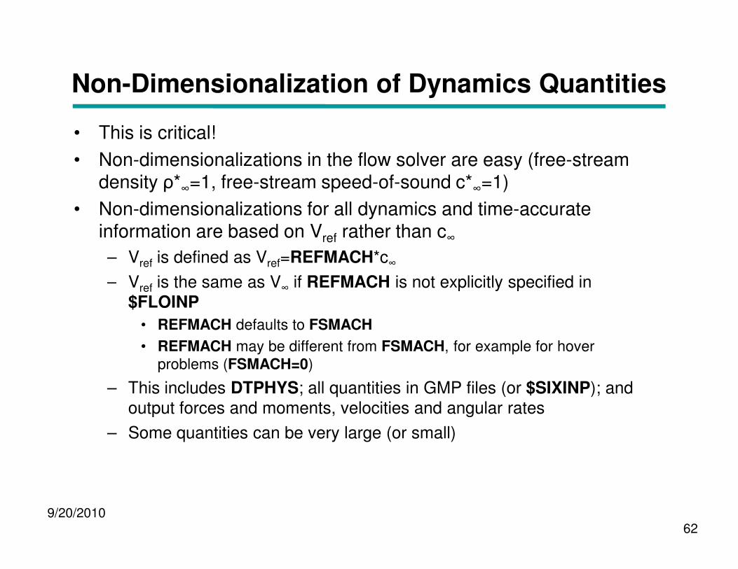
Non-Dimensionalization of Dynamics Quantities
• This is critical!
• Non-dimensionalizations in the flow solver are easy (free-stream density ρ*∞=1, free-stream speed-of-sound c*∞=1)
• Non-dimensionalizations for all dynamics and time-accurate information are based on Vref rather than c∞– Vref is defined as Vref=REFMACH*c∞– Vref is the same as V∞ if REFMACH is not explicitly specified in
9/20/201062
– Vref is the same as V∞ if REFMACH is not explicitly specified in $FLOINP
• REFMACH defaults to FSMACH
• REFMACH may be different from FSMACH, for example for hover problems (FSMACH=0)
– This includes DTPHYS; all quantities in GMP files (or $SIXINP); and output forces and moments, velocities and angular rates
– Some quantities can be very large (or small)

Non-Dimensionalization of Dynamics Quantities
• Non-dimensionalizations of dynamic quanities are thus based on
– Length: L=1 grid unit
– Time: L/Vref
– Mass: ρ∞L3
• Indicating non-dimensional quantities with a *:
– Length: len* = len / L
– Mass: m* = m / (ρ∞L3)
– Velocity: V* = V / V
9/20/201063
– Velocity: V* = V / Vref
– Time: t* = t (Vref/L)
– Acceleration: a* = a (L/Vref2)
– Force: F* = F / (ρ∞Vref2L2)
– Moment of inertia: I* = I / (ρ∞L5)
– Angular velocity: ω* = ω (L/Vref)
– Moment: M* = M / (ρ∞Vref2L3)
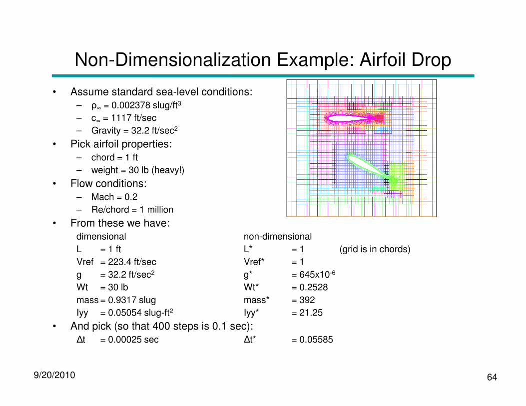
Non-Dimensionalization Example: Airfoil Drop
• Assume standard sea-level conditions:– ρ∞ = 0.002378 slug/ft3
– c∞ = 1117 ft/sec
– Gravity = 32.2 ft/sec2
• Pick airfoil properties:– chord = 1 ft
– weight = 30 lb (heavy!)
• Flow conditions:– Mach = 0.2
9/20/2010 64
– Re/chord = 1 million
• From these we have:dimensional non-dimensional
L = 1 ft L* = 1 (grid is in chords)
Vref = 223.4 ft/sec Vref* = 1
g = 32.2 ft/sec2 g* = 645x10-6
Wt = 30 lb Wt* = 0.2528
mass = 0.9317 slug mass* = 392
Iyy = 0.05054 slug-ft2 Iyy* = 21.25
• And pick (so that 400 steps is 0.1 sec):∆t = 0.00025 sec ∆t* = 0.05585
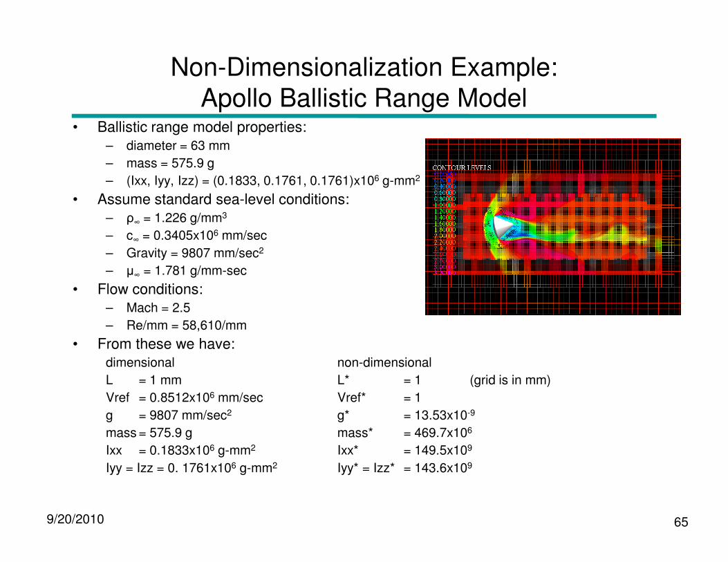
Non-Dimensionalization Example: Apollo Ballistic Range Model
• Ballistic range model properties:– diameter = 63 mm
– mass = 575.9 g
– (Ixx, Iyy, Izz) = (0.1833, 0.1761, 0.1761)x106 g-mm2
• Assume standard sea-level conditions:– ρ∞ = 1.226 g/mm3
– c∞ = 0.3405x106 mm/sec
– Gravity = 9807 mm/sec2
– µ∞ = 1.781 g/mm-sec
• Flow conditions:
9/20/2010 65
• Flow conditions:– Mach = 2.5
– Re/mm = 58,610/mm
• From these we have:dimensional non-dimensional
L = 1 mm L* = 1 (grid is in mm)
Vref = 0.8512x106 mm/sec Vref* = 1
g = 9807 mm/sec2 g* = 13.53x10⁻⁹
mass = 575.9 g mass* = 469.7x10⁶
Ixx = 0.1833x10⁶ g-mm2 Ixx* = 149.5x10⁹
Iyy = Izz = 0. 1761x106 g-mm2 Iyy* = Izz* = 143.6x10⁹
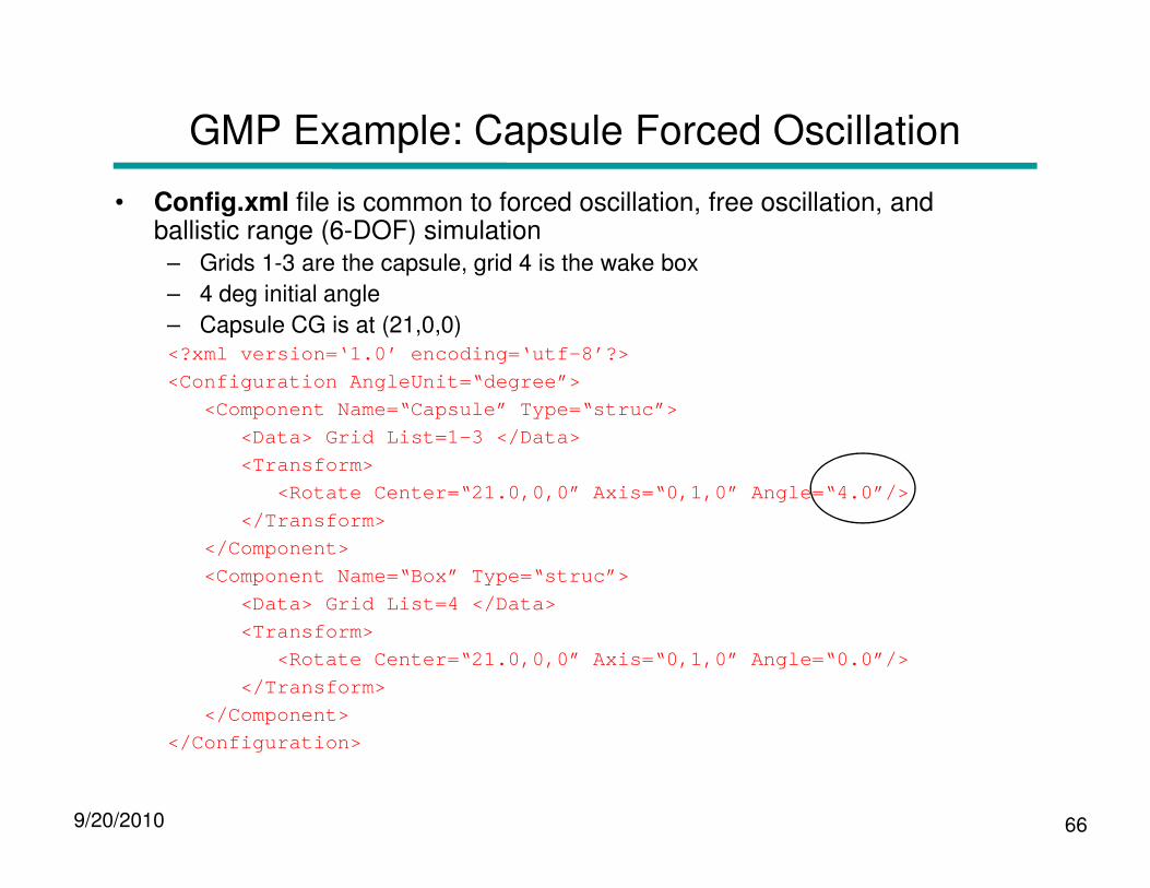
GMP Example: Capsule Forced Oscillation
• Config.xml file is common to forced oscillation, free oscillation, and ballistic range (6-DOF) simulation
– Grids 1-3 are the capsule, grid 4 is the wake box
– 4 deg initial angle
– Capsule CG is at (21,0,0)<?xml version=‘1.0’ encoding=‘utf-8’?>
<Configuration AngleUnit=“degree”>
<Component Name=“Capsule” Type=“struc”>
<Data> Grid List=1 - 3 </Data>
9/20/2010 66
<Data> Grid List=1 - 3 </Data>
<Transform>
<Rotate Center=“21.0,0,0” Axis=“0,1,0” Angle=“4.0”/ >
</Transform>
</Component>
<Component Name=“Box” Type=“struc”>
<Data> Grid List=4 </Data>
<Transform>
<Rotate Center=“21.0,0,0” Axis=“0,1,0” Angle=“0.0”/ >
</Transform>
</Component>
</Configuration>
GMP Example: Capsule Forced Oscillation
• Scenario.xml file for forced oscillation
– Time period for 1 oscillation is 20100 (non-dimensionalized)<?xml version=‘1.0’ encoding=‘utf-8’?>
<Scenario Name=“Forced Oscillation” AngleUnit=“degr ee”>
<Prescribed Component=“Capsule” Start=“0” >
<Rotate Center=“21.0,0,0” Axis=“0,1,0”
Speed=“4.*2.*pi/20100.*cos(2.*pi/20100.*t+pi/2.)”
Frame=“parent” />
9/20/201067
Frame=“parent” />
</Prescribed>
</Scenario>
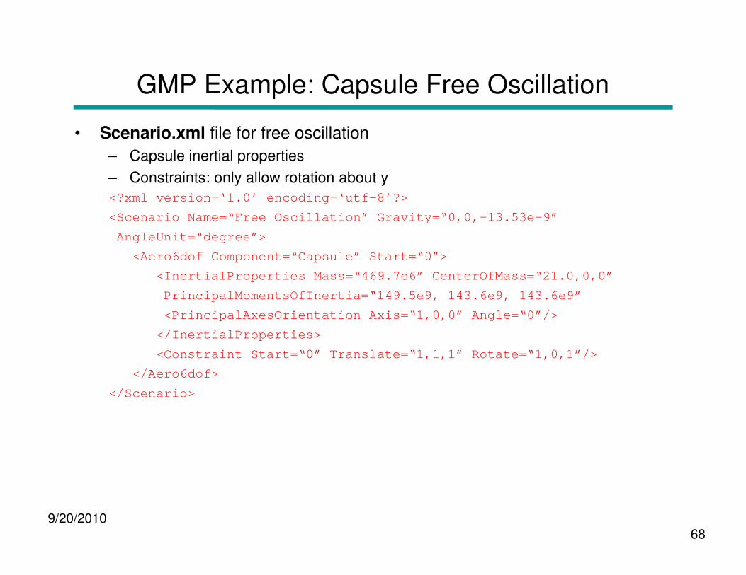
GMP Example: Capsule Free Oscillation
• Scenario.xml file for free oscillation
– Capsule inertial properties
– Constraints: only allow rotation about y
<?xml version=‘1.0’ encoding=‘utf-8’?>
<Scenario Name=“Free Oscillation” Gravity=“0,0,-13. 53e-9”
AngleUnit=“degree”>
<Aero6dof Component=“Capsule” Start=“0”>
<InertialProperties Mass=“469.7e6” CenterOfMass=“21 .0,0,0”
9/20/201068
PrincipalMomentsOfInertia=“149.5e9, 143.6e9, 143.6e 9”
<PrincipalAxesOrientation Axis=“1,0,0” Angle=“0”/>
</InertialProperties>
<Constraint Start=“0” Translate=“1,1,1” Rotate=“1,0 ,1”/>
</Aero6dof>
</Scenario>
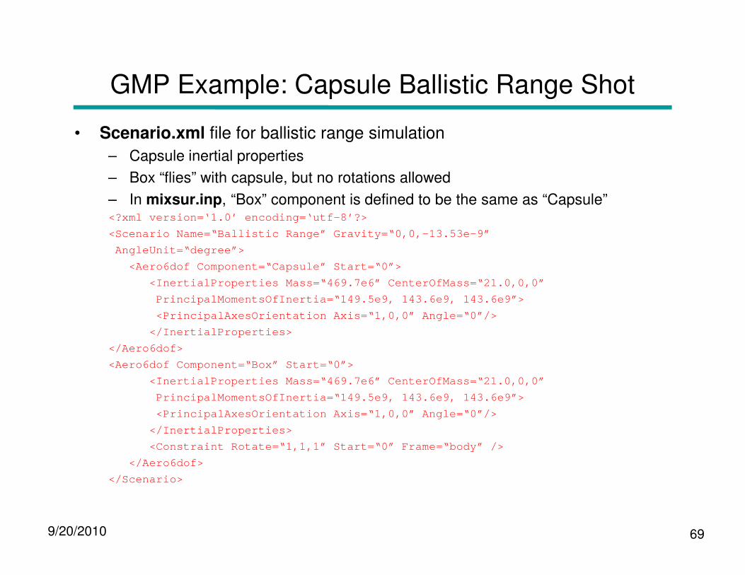
GMP Example: Capsule Ballistic Range Shot
• Scenario.xml file for ballistic range simulation
– Capsule inertial properties
– Box “flies” with capsule, but no rotations allowed
– In mixsur.inp, “Box” component is defined to be the same as “Capsule”<?xml version=‘1.0’ encoding=‘utf-8’?>
<Scenario Name=“Ballistic Range” Gravity=“0,0,-13.53e-9”
AngleUnit=“degree”>
<Aero6dof Component=“Capsule” Start=“0”>
<InertialProperties Mass=“469.7e6” CenterOfMass=“21.0,0,0”
9/20/2010 69
<InertialProperties Mass=“469.7e6” CenterOfMass=“21.0,0,0”
PrincipalMomentsOfInertia=“149.5e9, 143.6e9, 143.6e9”>
<PrincipalAxesOrientation Axis=“1,0,0” Angle=“0”/>
</InertialProperties>
</Aero6dof>
<Aero6dof Component=“Box” Start=“0”>
<InertialProperties Mass=“469.7e6” CenterOfMass=“21.0,0,0”
PrincipalMomentsOfInertia=“149.5e9, 143.6e9, 143.6e9”>
<PrincipalAxesOrientation Axis=“1,0,0” Angle=“0”/>
</InertialProperties>
<Constraint Rotate=“1,1,1” Start=“0” Frame=“body” />
</Aero6dof>
</Scenario>
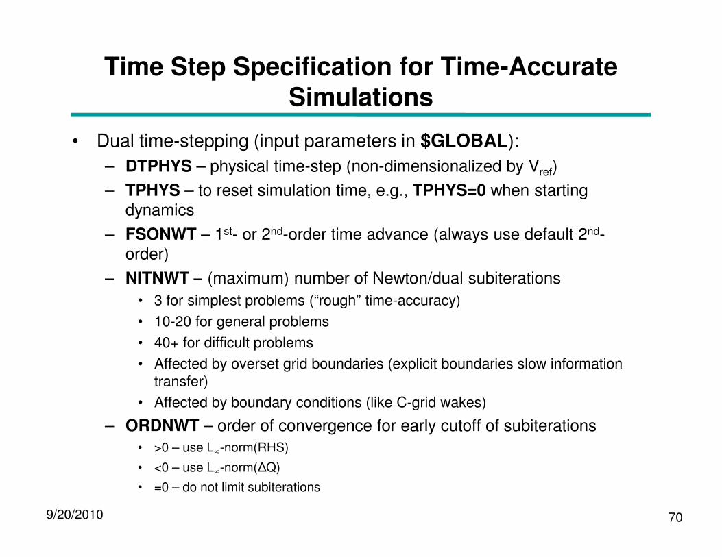
Time Step Specification for Time-Accurate Simulations
• Dual time-stepping (input parameters in $GLOBAL):
– DTPHYS – physical time-step (non-dimensionalized by Vref)
– TPHYS – to reset simulation time, e.g., TPHYS=0 when starting dynamics
– FSONWT – 1st- or 2nd-order time advance (always use default 2nd-order)
– NITNWT – (maximum) number of Newton/dual subiterations
9/20/2010 70
– NITNWT – (maximum) number of Newton/dual subiterations
• 3 for simplest problems (“rough” time-accuracy)
• 10-20 for general problems
• 40+ for difficult problems
• Affected by overset grid boundaries (explicit boundaries slow information transfer)
• Affected by boundary conditions (like C-grid wakes)
– ORDNWT – order of convergence for early cutoff of subiterations
• >0 – use L∞-norm(RHS)
• <0 – use L∞-norm(∆Q)
• =0 – do not limit subiterations
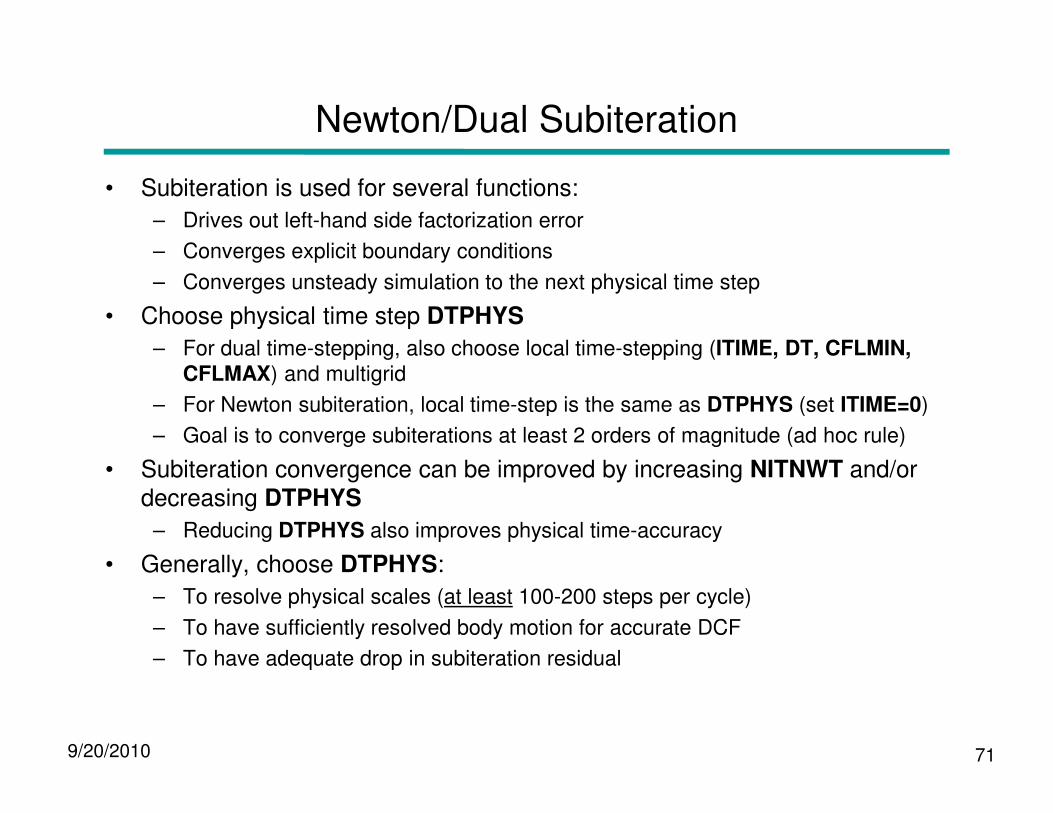
Newton/Dual Subiteration
• Subiteration is used for several functions:
– Drives out left-hand side factorization error
– Converges explicit boundary conditions
– Converges unsteady simulation to the next physical time step
• Choose physical time step DTPHYS
– For dual time-stepping, also choose local time-stepping (ITIME, DT, CFLMIN, CFLMAX) and multigrid
– For Newton subiteration, local time-step is the same as DTPHYS (set ITIME=0)
9/20/2010 71
– For Newton subiteration, local time-step is the same as DTPHYS (set ITIME=0)
– Goal is to converge subiterations at least 2 orders of magnitude (ad hoc rule)
• Subiteration convergence can be improved by increasing NITNWT and/or decreasing DTPHYS
– Reducing DTPHYS also improves physical time-accuracy
• Generally, choose DTPHYS:
– To resolve physical scales (at least 100-200 steps per cycle)
– To have sufficiently resolved body motion for accurate DCF
– To have adequate drop in subiteration residual

Converging Newton/Dual Subiterations
• In residual history files (resid.out, etc.) there is one entry (for each grid, or off-body grid level) per subiteration
• First subiteration right-hand side (RHS) residual represents the unsteady forcing function
– If this is decreasing (converging), the flow is becoming more steady
• The drop in RHS residual from first to last subiteration represents the numerical accuracy of computing the unsteady flow
– This should be at least 2 orders-of-magnitude (unless the flow is steady)
9/20/2010 72
– This should be at least 2 orders-of-magnitude (unless the flow is steady)
– Try using ORDNWT=2 to do this
• If selected grids are not converging as well as others, try setting ITER=2 for those grids
• A 2-order-of-magnitude drop indicates that the time advance is numerically
converged; it does not guarantee that the physical time-step is small enough to resolve physical processes
• Use OVERPLOT from CGT to plot resid.out –type files, as well as subiteration convergence

Converging Newton/Dual Subiterations
9/20/201073

Simulating Collisions
• Contact between bodies is detected by using X-ray hole-cutting applied to surface grids of other bodies
• Contact detection is enabled (per body) by adding grid “0” to IGXLIST in X-ray cutter(s)
• Example: airfoil drop$XRINFO IDXRAY=1, IGXLIST=-1, XDELTA=0.04, $END
$XRINFO IDXRAY=2, IGXLIST=-1, XDELTA=0.04, $END
$XRINFO IDXRAY=1, IGXLIST=2,0, XDELTA=0.0, $END
9/20/201074
$XRINFO IDXRAY=1, IGXLIST=2,0, XDELTA=0.0, $END
$XRINFO IDXRAY=2, IGXLIST=1,0, XDELTA=0.0, $END
• Accurate geometric representation of collisions may require much finer X-rays than hole-cutting
– To keep DCF process from becoming very slow, can make collision X-rays separate from DCF X-rays
• R_COEF in $OMIGLB sets (global) coefficient of restitution
• Time of contact is accurate only to within DTPHYS
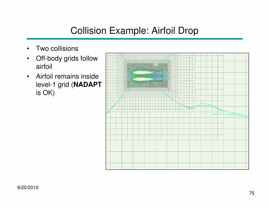
Collision Example: Airfoil Drop
• Two collisions
• Off-body grids follow airfoil
• Airfoil remains inside level-1 grid (NADAPTis OK)
9/20/201075
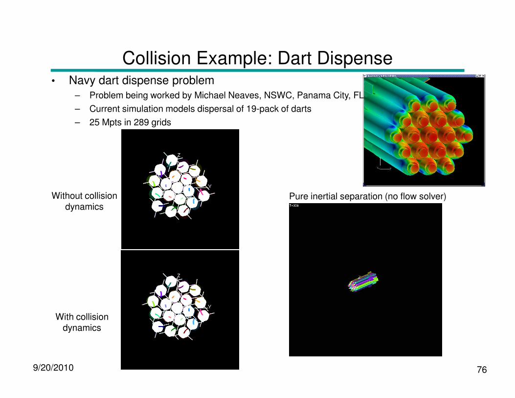
Collision Example: Dart Dispense• Navy dart dispense problem
– Problem being worked by Michael Neaves, NSWC, Panama City, FL
– Current simulation models dispersal of 19-pack of darts
– 25 Mpts in 289 grids
Without collision Pure inertial separation (no flow solver)
9/20/2010 76
Without collisiondynamics
With collisiondynamics
Pure inertial separation (no flow solver)

Output Information for Moving Body Simulations
• Input parameters in $GLOBAL:
– NSAVE – grid system, flow solution, and 6-DOF restart information is saved every NSAVE steps, as x.step#, q.step#, sixdof.step#
– NFOMO – force and moment coefficients are written to fomoco.out every NFOMO steps (automatically set to 1 for 6-DOF simulations)
• Namelist $SPLITM: write subsets of grid and solution every n steps (similar to CGT utilities SPLITMX, SPLITMQ)
• XFILE,QFILE,QAVGFILE – specify base names for grid, solution, and/or Q-
9/20/201077
• XFILE,QFILE,QAVGFILE – specify base names for grid, solution, and/or Q-average data (if blank, don’t write); step# will be appended to base name
• NSTART,NSTOP – start/stop step numbers for writing output files (use -1 for “last”)
• IPRECIS – output file precision (0—default,1—single, 2—double)
• IG(subset#) – subset grid number; use IG()=-1 for cut of all off-body grids
• JS,JE,JI,KS,KE,KI,LS,LE,LI(subset#) – subset ranges and increments
• CUT(subset#),VALUE(subset#) – off-body grid cut type (“x”, “y”, or “z”) and corresponding x, y, or z value
• Can have multiple $SPLITM namelists for multiple files
Output Information for Moving Body Simulations
• History files:
– fomoco.out – force and moment coefficients per component, per step (same as for static problems, except moment reference center moves with body)
– animate.out – body ID, physical time, body position and orientation (quaternion notation), velocity and rotation rates, aero forces and moments (not coefficients)
– contact.out – lists step #, body IDs, contact point and normal vector, reaction impulse, and linear and angular velocity changes (this is more for debugging collisions)
– Note that OVERRUN script concatenates these files into
9/20/201078
– Note that OVERRUN script concatenates these files into basename.{fomoco,animate,contact}
• Use OVERPLOT from CGT to plot fomoco.out, animate.out –type files
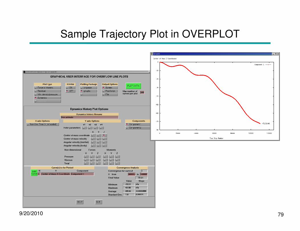
Sample Trajectory Plot in OVERPLOT
9/20/2010 79

Visualizing Body Motion in OVERGRID
• Prescribed motion can be visualized in OVERGRID by reading in (surface grids or) grid.in, Config.xml and Scenario.xml
– Start OVERGRID with surface grids or grid.in
– Click “COMPONENTS”
– On COMPONENTS menu,
• Click Read “Config” (“OK”)
• Click Read “Scenario” (“OK”)
9/20/2010 80
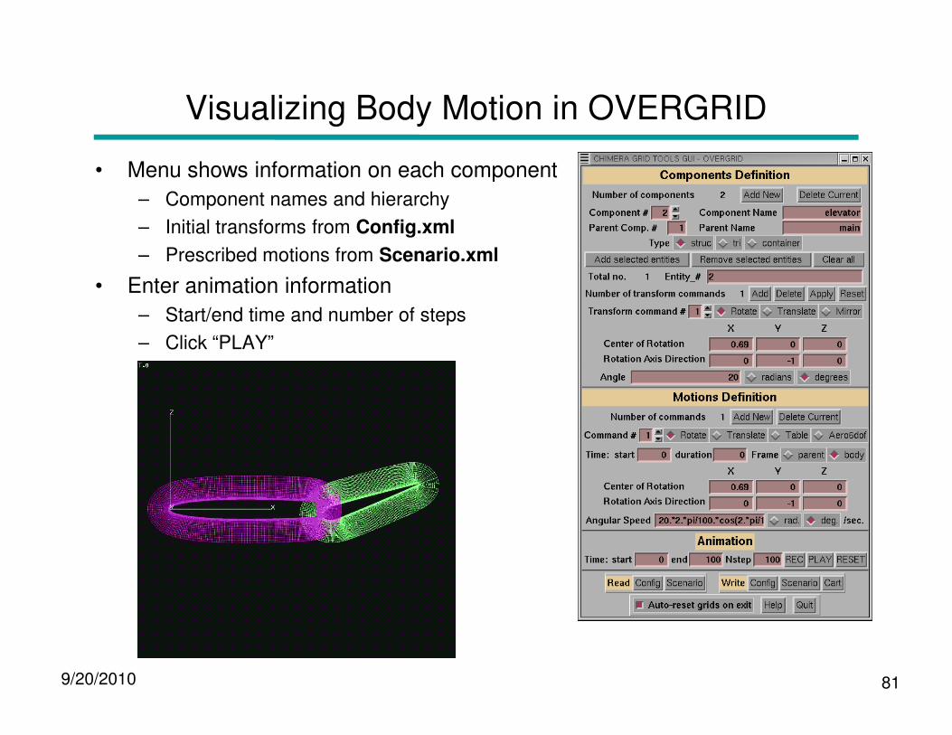
Visualizing Body Motion in OVERGRID
• Menu shows information on each component
– Component names and hierarchy
– Initial transforms from Config.xml
– Prescribed motions from Scenario.xml
• Enter animation information
– Start/end time and number of steps
– Click “PLAY”
9/20/2010 81

Visualizing Body Motion in OVERGRID
• For visualizing 6-DOF motion (after the OVERFLOW simulation is complete) read in basename.animate:
– Click “Add New” motion command
– Click “Table”
– Type in animate filename and click “Read”
– Click “PLAY”
9/20/2010 82
Some References
• GMP interface– S.M. Murman, W.M. Chan, M.J. Aftosmis, and R.L. Meakin, “An Interface for Specifying
Rigid-Body Motions for CFD Applications,” AIAA 2003-1237, Jan. 2003
• Solution adaption– R.L. Meakin, “An Efficient Means of Adaptive Refinement Within Systems of Overset Grids,”
AIAA 95-1722, June 1995
– R.L. Meakin, “On Adaptive Refinement and Overset Structured Grids,” AIAA 97-1858, June 1997
• Hole cutting using X-rays
9/20/2010 83
• Hole cutting using X-rays– R.L. Meakin, “Object X-Rays for Cutting Holes in Composite Overset Structured Meshes,”
AIAA 2001-2537, June 2001
• Off-body grid generation– R.L. Meakin, “Automatic Off-Body Grid Generation for Domains of Arbitrary Size,” AIAA
2001-2536, June 2001
• Collision dynamics– R.L. Meakin, “Multiple-Body Proximate-Flight Simulation Methods,” AIAA 2005-4621, June
2005

Solution Adaption for Off-Body Grids
• Allows off-body refinement grids that are finer than level-1
• Refinement levels are labelled -1, -2, etc., and have grid spacing of DS/2, DS/4, etc.
• Can be used with or without grid motion, for steady-state or time-accurate simulations
9/20/201084
400 steps, no adaption Additional 100 steps,adapting every 10 steps
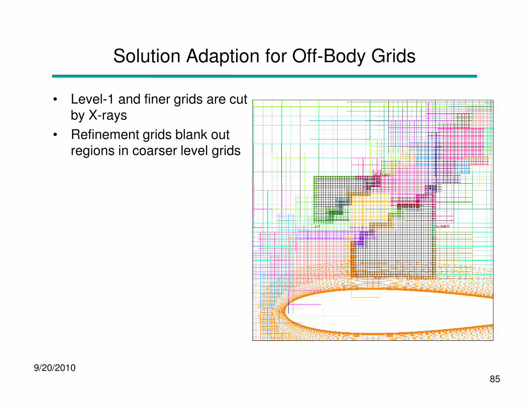
Solution Adaption for Off-Body Grids
• Level-1 and finer grids are cut by X-rays
• Refinement grids blank out regions in coarser level grids
9/20/201085

Input Parameters
• Basic control parameters (in $OMIGLB)
– NADAPT=n – adapt solution every n steps
• 0—do not adapt
• >0—adapt to geometry and sensor function
• <0—adapt to geometry only
– NREFINE=m – allow up to m levels of refinement
– ETYPE – sensor function for adaption
9/20/201086
• 0—undivided 2nd-difference of Q variables (squared)
• 1—vorticity magnitude
• 2—undivided vorticity magnitude
– EREFINE/ECOARSEN – refine above/coarsen below these function values
– SIGERR – shortcut method to set EREFINE and ECOARSEN
• EREFINE=(1/8)SIGERR, ECOARSEN=(1/8)SIGERR+2
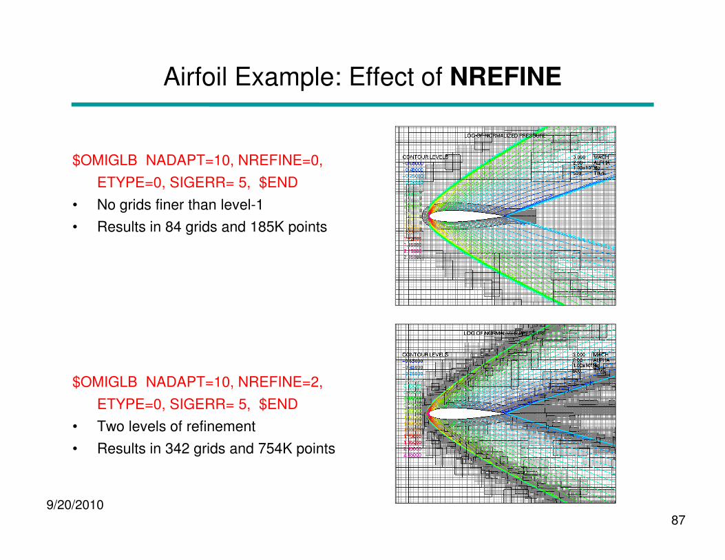
Airfoil Example: Effect of NREFINE
$OMIGLB NADAPT=10, NREFINE=0,
ETYPE=0, SIGERR= 5, $END
• No grids finer than level-1
• Results in 84 grids and 185K points
9/20/201087
$OMIGLB NADAPT=10, NREFINE=2,
ETYPE=0, SIGERR= 5, $END
• Two levels of refinement
• Results in 342 grids and 754K points
Input Parameters
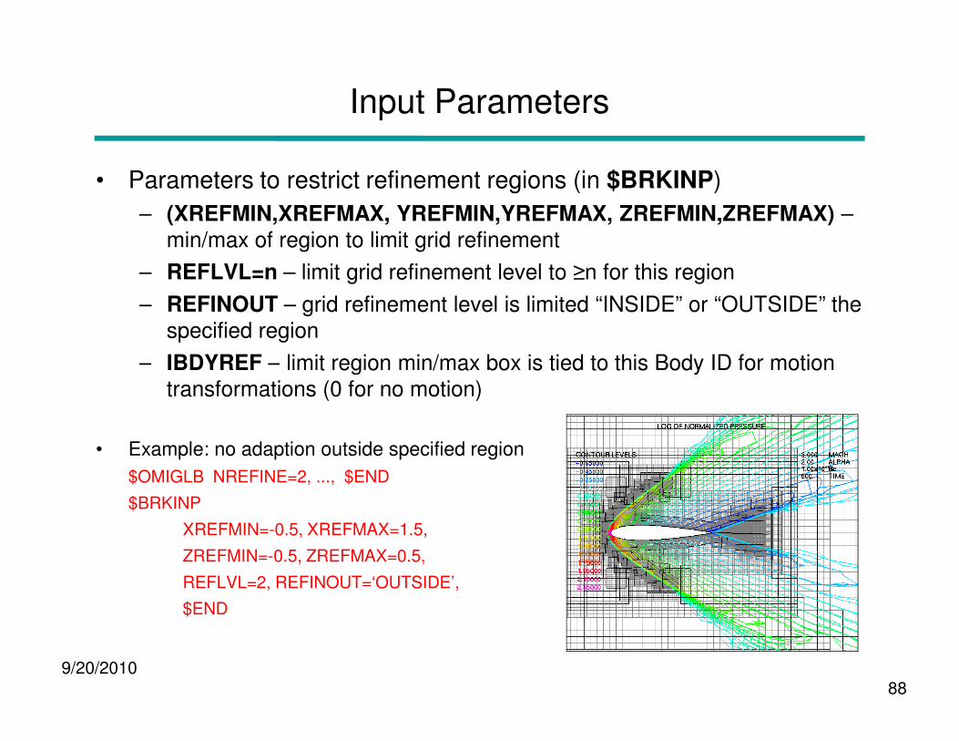
• Parameters to restrict refinement regions (in $BRKINP)
– (XREFMIN,XREFMAX, YREFMIN,YREFMAX, ZREFMIN,ZREFMAX) –min/max of region to limit grid refinement
– REFLVL=n – limit grid refinement level to ≥n for this region
– REFINOUT – grid refinement level is limited “INSIDE” or “OUTSIDE” the specified region
– IBDYREF – limit region min/max box is tied to this Body ID for motion
9/20/201088
– IBDYREF – limit region min/max box is tied to this Body ID for motion transformations (0 for no motion)
• Example: no adaption outside specified region
$OMIGLB NREFINE=2, ..., $END
$BRKINP
XREFMIN=-0.5, XREFMAX=1.5,
ZREFMIN=-0.5, ZREFMAX=0.5,
REFLVL=2, REFINOUT=‘OUTSIDE’,
$END
Notes and Comments
• Be careful of too many points!
• For time-accurate simulations, adjust NADAPT to make sure that adapted regions keep up with flow features and geometry
• Because the adaption can generate a large number of small grids, time-accurate simulations may need (more) subiterations to ensure good communication across grid boundaries
9/20/201089
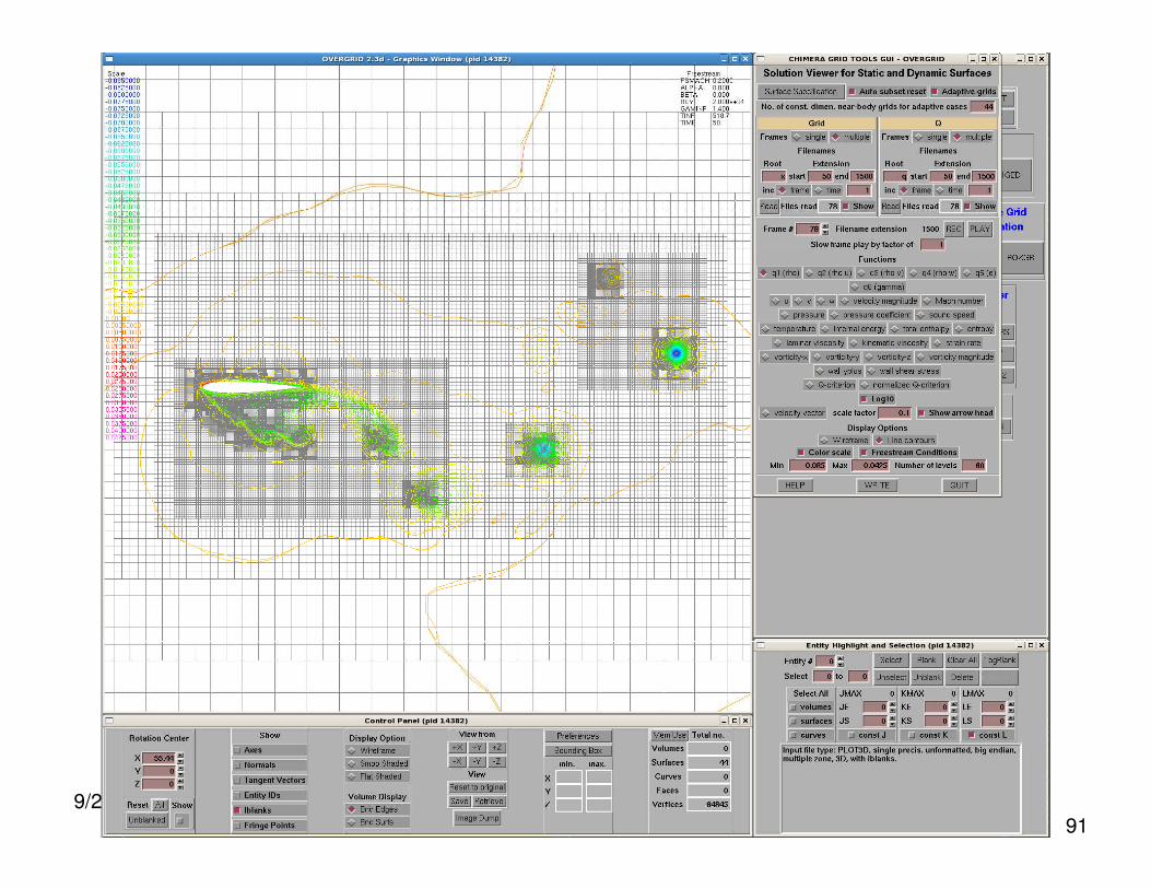
Visualizing Moving and/or Adapting Grids and Solutions using OVERGRID
• Moving or adapting (surface or 2D) grids can be visualized in OVERGRID by using the SOLUTION button (under “Viewers and Special Modules”)
– Start OVERGRID with x.save (or some grid)
– Click “SOLUTION”
– On SOLUTION menu,
• Click “Adaptive grids”
• Click “multiple”
9/20/201090
• Click “multiple”
• Adjust Root name, start, end
• Click “Read”
• Same for Q
• Select Function
• Click “PLAY” or step through frames
9/20/201091
Compiling and Running OVERFLOW
9/20/201092
• Unpacking and compiling
• Execution scripts
• Parallel processing and MPI load-balancing
• Hints and warnings
• Utility codes
• Test cases included with OVERFLOW
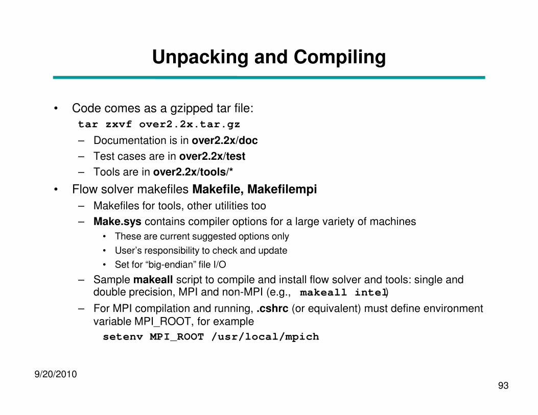
Unpacking and Compiling
• Code comes as a gzipped tar file:tar zxvf over2.2x.tar.gz
– Documentation is in over2.2x/doc
– Test cases are in over2.2x/test
– Tools are in over2.2x/tools/*
• Flow solver makefiles Makefile, Makefilempi
– Makefiles for tools, other utilities too
9/20/201093
– Makefiles for tools, other utilities too
– Make.sys contains compiler options for a large variety of machines
• These are current suggested options only
• User’s responsibility to check and update
• Set for “big-endian” file I/O
– Sample makeall script to compile and install flow solver and tools: single and double precision, MPI and non-MPI (e.g., makeall intel )
– For MPI compilation and running, .cshrc (or equivalent) must define environment variable MPI_ROOT, for example
setenv MPI_ROOT /usr/local/mpich
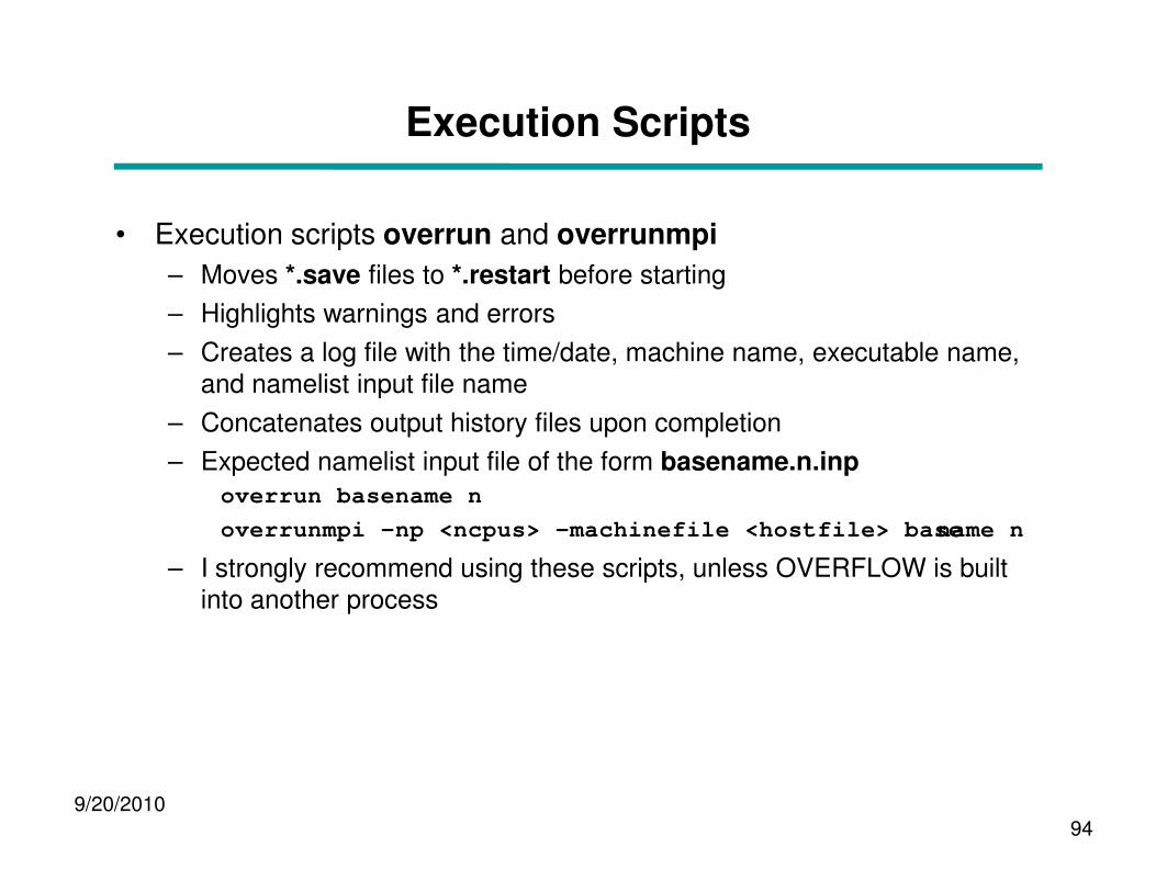
Execution Scripts
• Execution scripts overrun and overrunmpi
– Moves *.save files to *.restart before starting
– Highlights warnings and errors
– Creates a log file with the time/date, machine name, executable name, and namelist input file name
– Concatenates output history files upon completion
basename.n.inp
9/20/201094
– Expected namelist input file of the form basename.n.inp
overrun basename n
overrunmpi –np <ncpus> –machinefile <hostfile> base name n
– I strongly recommend using these scripts, unless OVERFLOW is built into another process
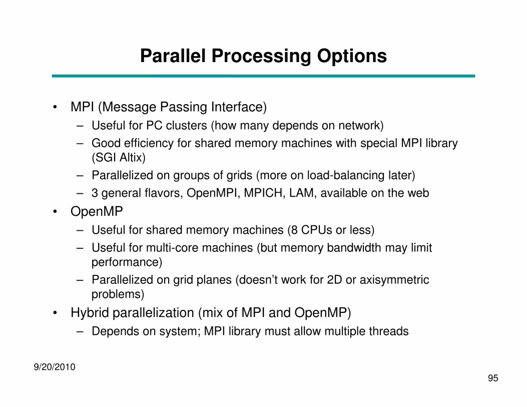
Parallel Processing Options
• MPI (Message Passing Interface)
– Useful for PC clusters (how many depends on network)
– Good efficiency for shared memory machines with special MPI library (SGI Altix)
– Parallelized on groups of grids (more on load-balancing later)
– 3 general flavors, OpenMPI, MPICH, LAM, available on the web
9/20/201095
• OpenMP
– Useful for shared memory machines (8 CPUs or less)
– Useful for multi-core machines (but memory bandwidth may limit performance)
– Parallelized on grid planes (doesn’t work for 2D or axisymmetricproblems)
• Hybrid parallelization (mix of MPI and OpenMP)
– Depends on system; MPI library must allow multiple threads
MPI Load-Balancing
• Number of groups == number of processes in the MPI run
• Default load-balancing scheme:
– Based on equal distribution of grid points between processes (target group size)
– Grids are split in half (with overlap added) until each grid is less than half the target group size
– Grids are distributed, from largest to smallest, to current smallest group
9/20/201096
– Grids are distributed, from largest to smallest, to current smallest group
– This scheme works quite well for grid systems with large numbers of grids, and reasonably well for smaller systems
– Some pathological cases:
• 1 grid, 2 processes (grid is split into 4 instead of 2)
• 1 grid, 3 processes (grid is split into 8, load-balance is 3/8,3/8,2/8)
– Note that grid splitting introduces additional explicit boundaries, which affects convergence behavior
MPI Load-Balancing
• Controlling load-balancing (input parameters in $GROUPS and $GLOBAL):
– Use of the following inputs is rarely needed
– USEFLE=.TRUE. – use previous timing information in grdwghts.restart for distributing grids to groups (FALSE – use default load-balancing scheme)
• Same as GRDWTS in $GLOBAL
– WGHTNB – weighting factor for near-body grids vs. off-body grids in default load-balancing scheme (for example if viscous terms are turned off in off-body grids)
9/20/2010 97
– MAXNB – control splitting of near-body grids
• MAXNB=0 – use automatic splitting algorithm
• MAXNB>0 – specified (weighted) size limit
• MAXNB<0 – do not split grids
• Same as MAX_GRID_SIZE in $GLOBAL
– MAXGRD – control splitting of off-body grids (same options as MAXNB)
– IGSIZE – maximum group size during grid adaption (default is 10Mpts)
– Example: pathological case 1 (single grid (1 million points), 2 processes)
• $GROUPS MAXNB=600000, $END
• Grid will be split once, with both halves smaller than 600,000 pts
• Each process will get one piece
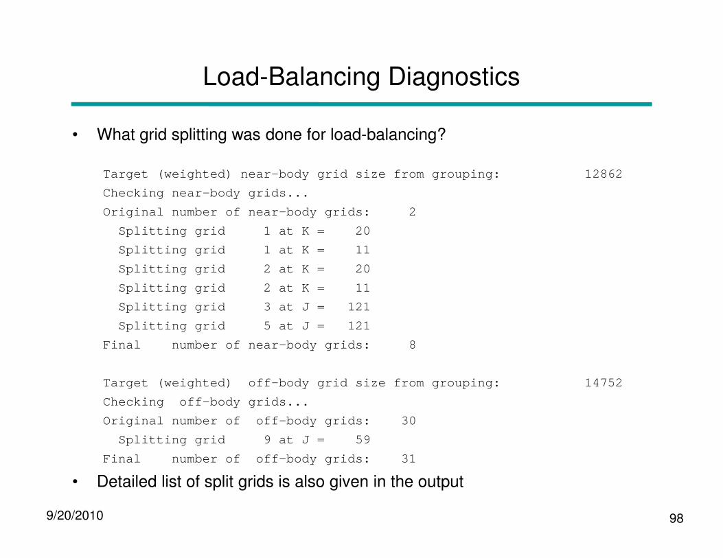
Load-Balancing Diagnostics
• What grid splitting was done for load-balancing?
Target (weighted) near-body grid size from grouping : 12862
Checking near-body grids...
Original number of near-body grids: 2
Splitting grid 1 at K = 20
Splitting grid 1 at K = 11
Splitting grid 2 at K = 20
9/20/2010 98
Splitting grid 2 at K = 11
Splitting grid 3 at J = 121
Splitting grid 5 at J = 121
Final number of near-body grids: 8
Target (weighted) off-body grid size from grouping : 14752
Checking off-body grids...
Original number of off-body grids: 30
Splitting grid 9 at J = 59
Final number of off-body grids: 31
• Detailed list of split grids is also given in the output

Load-Balancing Diagnostics
• What is the resulting grouping of grids?
Load balance will be based on grid size.
Summary of work distribution for 4 groups:
Group Kpts %load Grid list
1 30 100 4 8 11 17 14 22 21 33 31 34
9/20/2010 99
39
2 29 99 6 7 12 19 13 18 20 32 26 37
3 30 100 1 9 3 23 24 28 30 35 38
4 30 100 2 10 5 15 25 29 27 36 16
Predicted parallel efficiency is 100%,
based on a maximum of 30K grid points per group
compared to an average of 30K points (weighted)
Estimated parallel speedup is 4.0
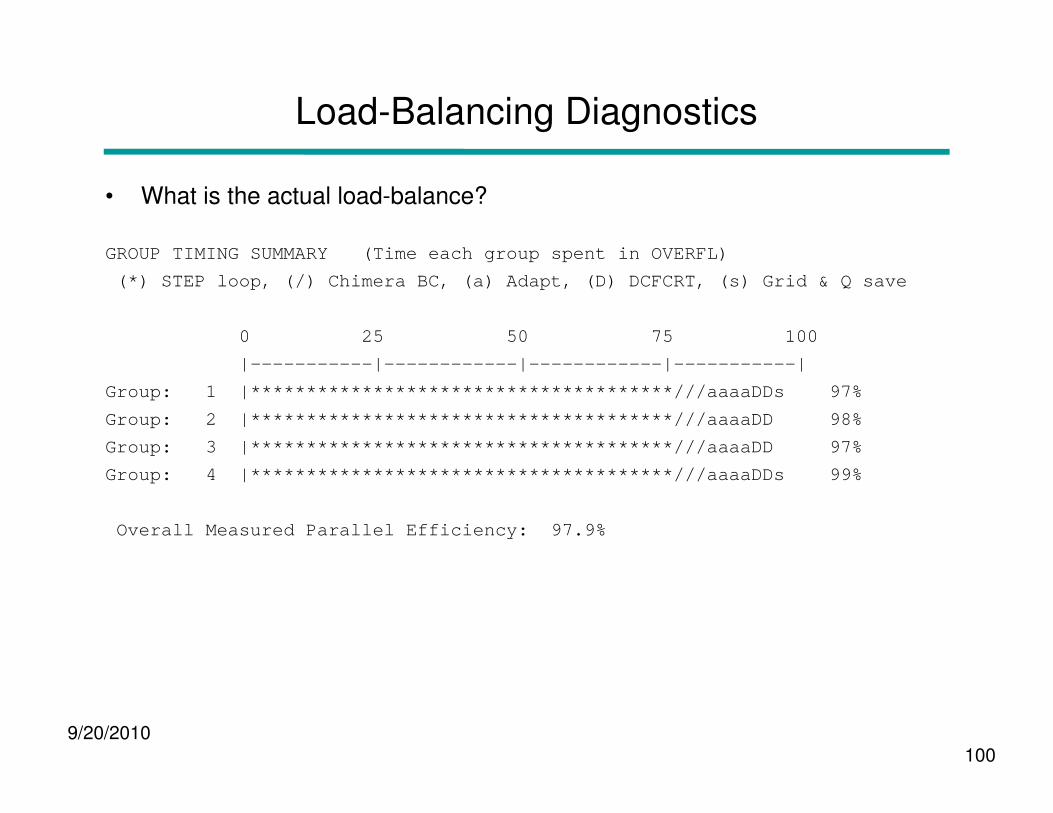
Load-Balancing Diagnostics
• What is the actual load-balance?
GROUP TIMING SUMMARY (Time each group spent in OV ERFL)
(*) STEP loop, (/) Chimera BC, (a) Adapt, (D) DCFCR T, (s) Grid & Q save
0 25 50 75 10 0
|-----------|------------|------------|-----------|
Group: 1 |************************************** ///aaaaDDs 97%
9/20/2010100
Group: 2 |************************************** ///aaaaDD 98%
Group: 3 |************************************** ///aaaaDD 97%
Group: 4 |************************************** ///aaaaDDs 99%
Overall Measured Parallel Efficiency: 97.9%
Load-Balancing – What to Look For
• Predicted parallel efficiency is lowPredicted parallel efficiency is 75%
– Not able to split or group grids effectively
– Some grids may not be split because of boundary conditions (axis, C-grid wake)– Change the number of CPUs or manually split problem grid
• Histogram shows groups are not well balancedGroup: 1 |************************************** *******///s 97%Group: 2 |**********************/// 47%
9/20/2010 101
Group: 3 |**********************/// 47%Group: 4 |**********************///s 49%
– Group 1 is sharing the CPU with another process– Eliminate other process or use a different CPU
• Large amount of time (~50%) spent exchanging Chimera BCsGroup: 1 |***********************/////////////// //////////s 98%Group: 2 |**********************//////////////// ////////// 96%Group: 3 |**********************//////////////// ////////// 97%Group: 4 |**********************//////////////// //////////s 99%
– Network is too slow to permit efficient use of this many CPUs
– Use fewer CPUs
Load-Balancing – What to Look For
• Measured parallel efficiency is less than predicted efficiency (5-10%)Predicted parallel efficiency is 96%
. . .0 25 50 75 100|-----------|------------|------------|-----------|
Group: 1 |*************************************//DDD 87%Group: 2 |***********************************//DDD 85%Group: 3 |**********************************//DDD 82%Group: 4 |***********************************///DDD 84%Group: 5 |***********************************//DDD 84%
. . .Group: 26 |*******************************************//DDD 99%
9/20/2010102
Group: 26 |*******************************************//DDD 99%Group: 27 |******************************************//DDD 97%Group: 28 |******************************************//DDD 98%Group: 29 |*****************************************//DDD 96%Group: 30 |*****************************************//DDD 96%Group: 31 |*****************************************//DDD 97%Group: 32 |*****************************************//DDD 97%
Overall Measured Parallel Efficiency: 92.4%
– Set USEFLE=.TRUE. to use timing from previous run for load-balancing
– This may improve the performance SOME

Hints and Warnings
• Unexplained errors while reading grid.in or q.restart file: check that all input files are the correct precision, correct “endian”, and match the executable being run
• Unexplained segmentation violation while running (Intel Linux machines?): available stack memory has been exceeded, add “limit stacksize unlimited” in .cshrc file
• “overflow killed” message on console: process ran out of memory, check
9/20/2010103
• “overflow killed” message on console: process ran out of memory, check problem size
Utilities and Test Cases
9/20/2010104
• Utility codes and more utility codes
• Test cases included with OVERFLOW
Utility Codes
• Chimera Grid Tools (CGT version 2.1)
– Grid generation and manipulation utilities
– Scripting process for grid generation and assembly
– Force & moment integration: mixsur, overint, USURP
– Post-processing utilities, OVERPLOT
– OVERGRID user interface
– Available from William Chan and Stuart Rogers, NASA Ames
9/20/2010105
– Available from William Chan and Stuart Rogers, NASA Ames (http://www.nas.nasa.gov/~rogers/home.html)
Utility Codes
OVERBUG, OVERTIME utility codes replaced by DEBUG input parameter in
$GLOBAL:
• DEBUG=1 – turbulence information quantities
– Surface quantities: wall spacing, y+, turbulence index
– Field quantities: µt, vorticity, damping functions, k, , etc.
– Different quantities per model—see OVERFLOW 2.2 manual, Section 6.1
– Data output in “fake” q file q.turb
• DEBUG=2 – time step information
9/20/2010106
• DEBUG=2 – time step information
– Field quantities: ∆t, J,K,L, and overall CFL#
– Data output in “fake” q file q.time
• DEBUG=3 – flow solver residual information
– Field quantities: flow solver residuals (right-hand side before time-step scaling)
– Data output in “fake” q file q.resid
• DEBUG=4 – solution adaption information
– Field quantities: sensor function, coarsen/refine marker array, log10(sensor fn)
– Data output in “fake” q file q.errest

Apollo Static Aero, Mach 1.2Mach number Turbulent eddy viscosity
Spalart-Allmaras
Max=25000
Turbulence model:
9/20/2010107
Baldwin-Barth
Laminar outsideboundary layer
Max=15000
Max=85
More Utility Codes
• Converting files between 32- and 64-bit– over2.2x/tools/run: grid32_to_64, etc.
• Converting files between big- and little-endian– Intel compiler environment flag F_UFMTENDIAN (select format per unit number)
– OVERGRID (for grid files)
– over2. 2x/tools/endian_convert
• Extracting or setting turbulence field quantities in a q file– over2. 2x/tools/turbulence: addbb, addke, bbplot
9/20/2010108
– over2. 2x/tools/turbulence: addbb, addke, bbplot
• Estimating viscous wall spacing– over2. 2x/tools/turbulence: find_y, find_y2
• Plotting flow quantities with variable gamma and/or multiple species– PLOT3D assumes a constant gamma=1.4, so thermodynamic quantities are not
correct
– over2. 2x/tools/variable_gamma/vgplot writes out fake q files with (pressure, temperature, Mach number, stagnation enthalpy, gamma), and (species mass fractions)
• Chemistry table for generating polynomial coefficients for variable gamma options in OVERFLOW (do not use!)
– over2. 2x/tools/chemistry: gaschem.f, fort.4
Utility Codes From Bobby Nichols
• Scan a q.save file for min/max density, pressure, temperature, Mach number
– over2.2x/tools/run/checkq
• Convert a q.save file between 1- and 2-equation turbulence models
– over2.2x/tools/turbulence/turb_init
• Calculate surface skin friction and heat transfer coefficients
– over2.2x/tools/unsupported/cfwf
9/20/2010109
– over2.2x/tools/unsupported/cfwf
• Create an fvbnd file for Fieldview
– over2.2x/tools/unsupported/fvbnd
Test Cases Included With OVERFLOW
• Simple 2D cases (steady flow, single grid):– flat_plate, flat_plate_high_re– flat_plate_wf (tests wall function skin friction)– shear_layer– driven_cavity_2d (low-Mach preconditioning test case)– curved_wall_2d (tests turbulence model curvature corrections)– 3gas (simple multiple species convection case)
• Transonic 2D or axisymmetric cases (steady flow, single grid):– bump (axisymmetric bump, shock-induced separation)
9/20/2010110
– bump (axisymmetric bump, shock-induced separation)– naca, naca4412, naca_ogrid– et_axi, srb_axi
• Hypersonic 2D cases (steady flow, single grid):– cylinder, cyl_holden (2D Mach 8,16 flow)
Test Cases, Continued
• 2D multiple grids:– af3_96 (multi-element airfoil)– cascade
• 2D moving body cases:– airfoil_drop_2d– rotating_paddle_2d– pitching_airfoil_2d
• Propulsion cases:– nozzle (rocket nozzle inflow/outflow boundary conditions)
9/20/2010111
– eggers, seiner (axisymmetric plume flows)– powered_nacelle (jet engine inflow/outflow boundary conditions)– normal_jet_2d (simple jet-in-crossflow)
• Classical time-accurate cases:
– shock_tube
– vortex_convection, vortex_convection_HiO, lambVortex_convection
– stokes_1st_problem (impulsively started plate)
– oscillating_sphere (acoustic test case)
Test Cases, Continued
• Subsonic/transonic 3D (steady, single grid):
– m2129_s_duct (S-duct inlet)
– rotating_disk (infinite rotating plate)
– onera_m6 (classic transonic wing test cases)
– inf_swept (infinite swept wing)
– ogive_cylinder
• Subsonic/transonic 3D (steady, multiple grid):
– wingbody (AGARD test case)
9/20/2010112
– wingbody (AGARD test case)
– bizjet (assembling and running a wing/body/pylon/nacelle)
– robin_sym (helicopter fuselage, illustrates some numerical problems)
• Off-body grid adaption cases:– airfoil_adapt (new)– normal_jet_adapt (simple jet-in-crossflow) (new)
Future Directions
• Near-term:
– Near-body solution-adaptive gridding
– Turbulence model with transition (Langtry-Menter SST)
• Longer-term:
– More robust moving body process
• adaptive time-step, subiteration control
– Improve flow solver robustness
9/20/2010113
– Improve flow solver robustness
• No dumping core or negative density/pressure
– Improve cache and multi-core performance
– Modularize for incorporation into (some form of) scripting framework