Embed Size (px)
Citation preview

Overcoming Interference II: MIMO and Interference Alignment
Kyle Jamieson UCL Computer Science
COMPM038/COMPGZ06 1st March 2013
Today
1. MIMO primer [802.11 with MulAple Antennas for Dummies, Halperin et al., ‘08]
2. Interference alignment and cancellaHon [Gollakota et al., SIGCOMM ’09]

MIMO: High-‐level view • Recall: MulApath reflecHons can impair performance
– Channel is composed of mulAple spaAal paths – Delayed copies of transmiSed symbols sum up and interfere with each other and surrounding symbols
• Mid ‘90s: Foschini, Gans, Telatar turn mulApath
propagaAon from impairment to an opportunity – Use mulHple antennas at sender (input) and at receiver (output) – Scale capacity linearly with numbers of antennas
Output: Channel input: x(t) y(t) = ai x(t −i∑ τ i )+w(t)τ3, a3
τ2, a2
Differing uses of MIMO
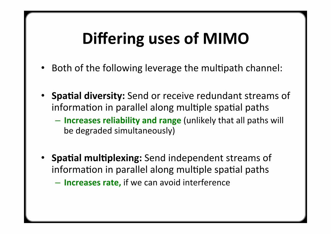
• Both of the following leverage the mulHpath channel:
• SpaAal diversity: Send or receive redundant streams of informaHon in parallel along mulHple spaHal paths – Increases reliability and range (unlikely that all paths will be degraded simultaneously)
• SpaAal mulAplexing: Send independent streams of informaHon in parallel along mulHple spaHal paths – Increases rate, if we can avoid interference
OFDM: MulAplexing in frequency
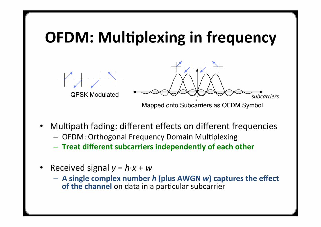
• MulHpath fading: different effects on different frequencies – OFDM: Orthogonal Frequency Domain MulHplexing – Treat different subcarriers independently of each other
• Received signal y = h·∙x + w – A single complex number h (plus AWGN w) captures the effect of the channel on data in a parHcular subcarrier
(5) QPSK Modulatedf
(6) Mapped onto Subcarriers as OFDM Symbol
Figure 1: A graphical view of the OFDM encoding process for the 18 Mbps rate (QPSK, 3/4) of 802.11a.The data bits (0) are encoded by a rate-1/2 convolutional code (1) and then optionally punctured by droppingcertain bits for higher coding rates (here, 3/4) that send fewer redundant bits (2). The remaining bits are in-terleaved (3) to spread the redundancy across subcarriers and protect against frequency-selective fades. Thesebits are grouped into symbols (4) based on the modulation (QPSK encodes 2 bits per symbol), modulated (5),and finally mapped onto the di↵erent subcarriers to form an OFDM symbol (6).
h11
h12
h11
h12y = x2
Tx Rx
y = xx
1
(a) Receive diversity
h11
h21
h11 h21
Tx Rx
x
x
( + ) xy =
y
(b) Transmit diversity
x1
x2
h11
h12h21
h22
h11x1 h21x2
h12x1 h22x2y2 = +
Tx Rx
y = 1 +
(c) Spatial multiplexing
Figure 2: Using some of the transmit/receive antennas in an example 2x2 system to exploit diversity andmultiplexing gain. xi and yi represent transmitted and received signals. The channel gain hij is a complexnumber indicating a signal’s attenuated amplitude and phase shift over the channel between the ith transmitantenna and the jth receive antenna. The received signals yi will additionally include thermal RF noise.
modulation sending more bits per symbol and being usedwhen there is a higher SNR. There are minor di↵erences be-tween 802.11a/g and 802.11n. In 802.11a/g there are 48 datasubcarriers, 4 pilot tones for control, and 6 unused guardsubcarriers at each edge of the channel. In 802.11n, thereare only 4 guard subcarriers at each edge of the channel, andtwo adjacent 20 MHz channels can be merged into a single40 MHz channel.
The beauty of OFDM is that it divides the channel in away that is both computationally and spectrally e�cient.High aggregate data rates can be achieved, while the en-coding and decoding on di↵erent subcarriers can use sharedhardware components. More relevant to our point here, how-ever, is that OFDM transforms a single large channel intomany relatively independently faded channels. This is be-cause multi-path fading is frequency selective, so the di↵er-ent subcarriers will experience di↵erent fades. Some adja-cent subcarriers may be faded in a similar way, but the fadingfor more distant subcarriers is often uncorrelated. Dividingthe channel also increases the symbol time per channel, sincemany slow symbols will be sent in parallel instead of manyfast symbols in sequence. This adds time diversity becausethe channel is more likely to average out fades over a longerperiod of time.
802.11 makes use of the frequency diversity provided byOFDM by coding across the data carried on the subcarriers.This uses a fraction of them for redundant information thatcan later be used to correct errors that occur when fadingreduces the SNR on some of the subcarriers. First, a con-
volutional code of rate 1/2 adds redundant information. Itis then punctured [3] by removing bits as needed to supportcoding rates of 2/3 and 3/4, plus 5/6 for 802.11n. At a rateof 3/4, for example, a quarter of the data on the subcarriersis redundant. An alternative LDPC (Low-Density Parity-Check) code with slightly better performance can also beused for 802.11n. Figure 1 presents a pictorial overview ofthe OFDM encoding process.
The net e↵ect of OFDM plus coding is to provide consis-tently good 802.11 performance despite significant variabil-ity in the wireless signal due to multi-path fading.
3. SPATIAL DIVERSITYIn this section we look at spatial diversity techniques that
can be applied at the receiver and at the transmitter. Addingmultiple antennas to an 802.11n receiver or transmitter pro-vides a new set of independently faded paths, even if theantennas are separated by only a few centimeters. Thisadds spatial diversity to the system, which can be exploitedto improve resilience to fades. There is also a power gainfrom multiple receive antennas because, everything else be-ing equal, two receive antennas will receive twice the signal.These factors combine to improve performance at a givendistance, and hence increase range.
3.1 Receive Diversity TechniquesConsider the arrangement in Figure 2(a). One transmit
antenna at a node is sending to two receive antennas at a
subcarriers
Mapping data bits to OFDM subcarriers
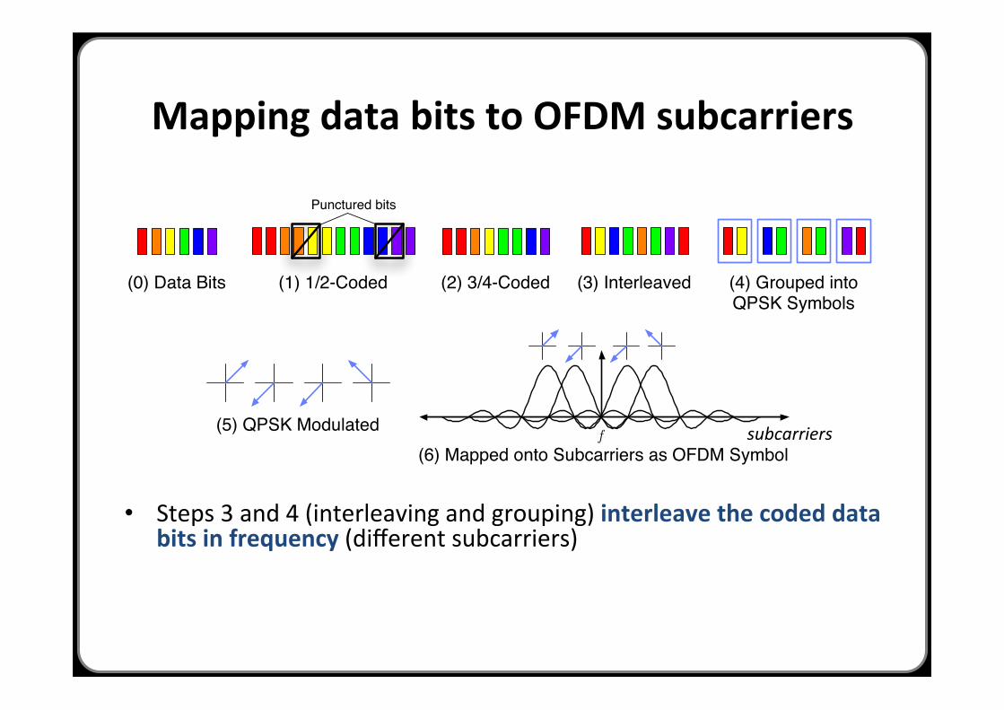
• Steps 3 and 4 (interleaving and grouping) interleave the coded data bits in frequency (different subcarriers)
(5) QPSK Modulatedf
(6) Mapped onto Subcarriers as OFDM Symbol
(0) Data Bits (2) 3/4-Coded (3) Interleaved (4) Grouped intoQPSK Symbols
(1) 1/2-Coded
Punctured bits
Figure 1: A graphical view of the OFDM encoding process for the 18 Mbps rate (QPSK, 3/4) of 802.11a.The data bits (0) are encoded by a rate-1/2 convolutional code (1) and then optionally punctured by droppingcertain bits for higher coding rates (here, 3/4) that send fewer redundant bits (2). The remaining bits are in-terleaved (3) to spread the redundancy across subcarriers and protect against frequency-selective fades. Thesebits are grouped into symbols (4) based on the modulation (QPSK encodes 2 bits per symbol), modulated (5),and finally mapped onto the di↵erent subcarriers to form an OFDM symbol (6).
h11
h12
h11
h12y = x2
Tx Rx
y = xx
1
(a) Receive diversity
h11
h21
h11 h21
Tx Rx
x
x
( + ) xy =
y
(b) Transmit diversity
x1
x2
h11
h12h21
h22
h11x1 h21x2
h12x1 h22x2y2 = +
Tx Rx
y = 1 +
(c) Spatial multiplexing
Figure 2: Using some of the transmit/receive antennas in an example 2x2 system to exploit diversity andmultiplexing gain. xi and yi represent transmitted and received signals. The channel gain hij is a complexnumber indicating a signal’s attenuated amplitude and phase shift over the channel between the ith transmitantenna and the jth receive antenna. The received signals yi will additionally include thermal RF noise.
modulation sending more bits per symbol and being usedwhen there is a higher SNR. There are minor di↵erences be-tween 802.11a/g and 802.11n. In 802.11a/g there are 48 datasubcarriers, 4 pilot tones for control, and 6 unused guardsubcarriers at each edge of the channel. In 802.11n, thereare only 4 guard subcarriers at each edge of the channel, andtwo adjacent 20 MHz channels can be merged into a single40 MHz channel.
The beauty of OFDM is that it divides the channel in away that is both computationally and spectrally e�cient.High aggregate data rates can be achieved, while the en-coding and decoding on di↵erent subcarriers can use sharedhardware components. More relevant to our point here, how-ever, is that OFDM transforms a single large channel intomany relatively independently faded channels. This is be-cause multi-path fading is frequency selective, so the di↵er-ent subcarriers will experience di↵erent fades. Some adja-cent subcarriers may be faded in a similar way, but the fadingfor more distant subcarriers is often uncorrelated. Dividingthe channel also increases the symbol time per channel, sincemany slow symbols will be sent in parallel instead of manyfast symbols in sequence. This adds time diversity becausethe channel is more likely to average out fades over a longerperiod of time.
802.11 makes use of the frequency diversity provided byOFDM by coding across the data carried on the subcarriers.This uses a fraction of them for redundant information thatcan later be used to correct errors that occur when fadingreduces the SNR on some of the subcarriers. First, a con-
volutional code of rate 1/2 adds redundant information. Itis then punctured [3] by removing bits as needed to supportcoding rates of 2/3 and 3/4, plus 5/6 for 802.11n. At a rateof 3/4, for example, a quarter of the data on the subcarriersis redundant. An alternative LDPC (Low-Density Parity-Check) code with slightly better performance can also beused for 802.11n. Figure 1 presents a pictorial overview ofthe OFDM encoding process.
The net e↵ect of OFDM plus coding is to provide consis-tently good 802.11 performance despite significant variabil-ity in the wireless signal due to multi-path fading.
3. SPATIAL DIVERSITYIn this section we look at spatial diversity techniques that
can be applied at the receiver and at the transmitter. Addingmultiple antennas to an 802.11n receiver or transmitter pro-vides a new set of independently faded paths, even if theantennas are separated by only a few centimeters. Thisadds spatial diversity to the system, which can be exploitedto improve resilience to fades. There is also a power gainfrom multiple receive antennas because, everything else be-ing equal, two receive antennas will receive twice the signal.These factors combine to improve performance at a givendistance, and hence increase range.
3.1 Receive Diversity TechniquesConsider the arrangement in Figure 2(a). One transmit
antenna at a node is sending to two receive antennas at a
subcarriers
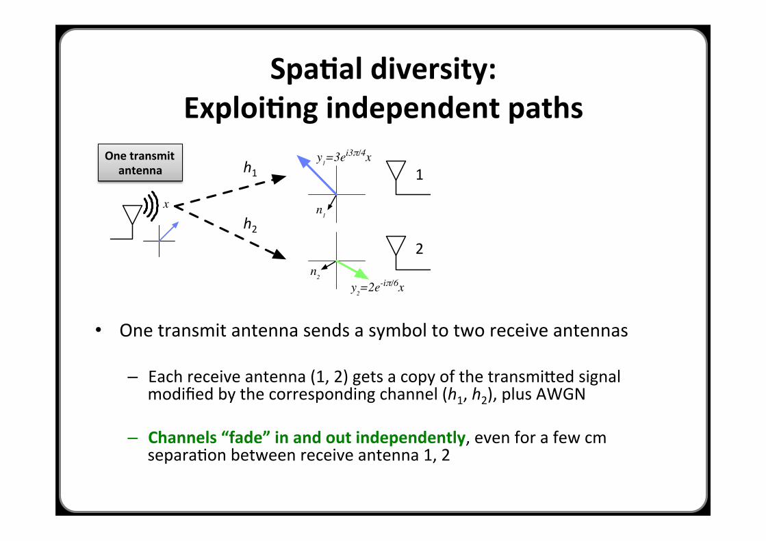
SpaAal diversity: ExploiAng independent paths
• One transmit antenna sends a symbol to two receive antennas
– Each receive antenna (1, 2) gets a copy of the transmiSed signal modified by the corresponding channel (h1, h2), plus AWGN
– Channels “fade” in and out independently, even for a few cm separaHon between receive antenna 1, 2
n2
y2=2e-iπ/6x
rotate, scale by 2/p
13
rotate, scale by 3/p
13
�
9/p
13
4/p
13
p13
x
n expected 1
y1=3ei3π/4x
n1
Figure 3: MRC operation on a sample channel. The channel gains are ~h = h3ei3⇡/4, 2e�i⇡/6i, with Gaussiannoise ~n = hn1, n2i of expected power 1. The antennas have respective SNRs of 9 and 4. To implement MRC,
the receiver multiplies the received signal ~y = ~hx + ~n by the unit vector ~h⇤/||~h||, where ~h⇤ denotes the complex
conjugate of ~h. This operation scales each antenna’s signal by its magnitude, and rotates the signals intothe same phase reference before adding them. (For graphical clarity, we depict the common phase vertically,rather than at 0). The resulting sum has magnitude
p13, and expected noise power 1 because the scaling is
normalized. Thus, by coherently combining received signals from di↵erent antennas, the MRC output hasthe expected SNR of 13. In systems with OFDM, MRC is performed separately for each subcarrier.
second node. This is known as a 1x2 system. Real systemsmay have more than two receive antennas, but two will suf-fice for our explanation. With this setup, each receive an-tenna receives a copy of the transmitted signal modified bythe channel between the transmitter and itself. The chan-nel gains hij are complex numbers that represent both theamplitude attenuation over the channel as well as the path-dependent phase shift (see Figure 3 for a graphical example).The receiver measures the channel gains based on trainingfields in the packet preamble. Note that the gains di↵er foreach subcarrier (in frequency-selective fading) as well as foreach antenna. The question now is how to combine the tworeceived signals to make best use of them.
We consider two diversity techniques to show the extremes.The simplest method is to use the antenna with the strongestsignal (hence the largest SNR) to receive the packet and ig-nore the others. We will call this method SEL, for selectioncombining. This is essentially what is done by 802.11a/g APswith multiple antennas. It helps with reliability, becauseboth signals are unlikely to be bad, but it wastes perfectlygood received power at the antennas that are not chosen.
The better method is to add the signals from the twoantennas together. However, this cannot be done by simplysuperimposing their signals, or we will have just recreatedthe e↵ects of multi-path fading. Rather, the signals shouldeach be delayed until they are in the same phase; then, thepower in the signals will combine coherently. To do this,the receiver needs a dedicated RF chain for each antenna toprocess the signals. This increases the hardware complexityand power consumption, but yields better performance.
As a twist in the above, the signals are also weighted bytheir SNRs. This gives less weight to a signal that has alarger fraction of noise, so that the e↵ects of the noise are notamplified. The result is maximal-ratio combining, or MRC.MRC is known to be optimal (it maximizes SIMO capacity),and produces an SNR that is the sum of the componentSNRs. Note that in frequency-selective fading, this processis performed di↵erently for each subcarrier according to itsspecific channel gains.
Figure 3 depicts MRC operation graphically for a 1x2channel. In this example, the two channel gains have magni-
-25
-20
-15
-10
-5
0
-20 -10 0 10 20
No
rma
lize
d p
ow
er
(dB
)
Subcarrier index
AC
B and SELAB (MRC)
ABC (MRC)
Figure 4: Frequency-selective fading over testbedlinks: the figure shows, for an example 5.2 GHz link,the received power measured on each subcarrier forindividual antennas and under SEL and MRC diver-sity, normalized to the strongest subcarrier power.
tudes of 3 and 2. With expected noise power 1, these gainscorrespond to SNRs of 9 and 4, given that a signal’s power isthe square of its magnitude. The MRC receiver scales eachantenna’s signal by its magnitude, normalized to the total;delays the signals to a common phase reference; and thenadds them. The result has magnitude
p13, and the normal-
ized weighted sum of noise still has expected power 1. Thecombined signal thus has a resulting sum SNR of 13.
As an example of how MRC and SEL work in 802.11, con-sider Figure 4. This figure shows the wireless signal strengthof each subcarrier using three antennas for a real 802.11n linkin our indoor wireless testbed. The subcarrier strengths aremeasured in decibels normalized to the strongest subcarrierstrength. This figure gives a much more detailed view thanmetrics such as the RSSI (Received Signal Strength Indi-cation) for a link, which gives only the sum of the signalstrength over all subcarriers.
For each antenna labeled A, B, or C, the signal variesover the channel, changing gradually from one subcarrier
One transmit antenna
Figure 1: A graphical view of the OFDM encoding process for the 18 Mbps rate (QPSK, 3/4) of 802.11a.The data bits (0) are encoded by a rate-1/2 convolutional code (1) and then optionally punctured by droppingcertain bits for higher coding rates (here, 3/4) that send fewer redundant bits (2). The remaining bits are in-terleaved (3) to spread the redundancy across subcarriers and protect against frequency-selective fades. Thesebits are grouped into symbols (4) based on the modulation (QPSK encodes 2 bits per symbol), modulated (5),and finally mapped onto the di↵erent subcarriers to form an OFDM symbol (6).
h11
h12
h11
h12y = x2
Tx Rx
y = xx
1
(a) Receive diversity
h11
h21
h11 h21
Tx Rx
x
x
( + ) xy =
y
(b) Transmit diversity
x1
x2
h11
h12h21
h22
h11x1 h21x2
h12x1 h22x2y2 = +
Tx Rx
y = 1 +
(c) Spatial multiplexing
Figure 2: Using some of the transmit/receive antennas in an example 2x2 system to exploit diversity andmultiplexing gain. xi and yi represent transmitted and received signals. The channel gain hij is a complexnumber indicating a signal’s attenuated amplitude and phase shift over the channel between the ith transmitantenna and the jth receive antenna. The received signals yi will additionally include thermal RF noise.
modulation sending more bits per symbol and being usedwhen there is a higher SNR. There are minor di↵erences be-tween 802.11a/g and 802.11n. In 802.11a/g there are 48 datasubcarriers, 4 pilot tones for control, and 6 unused guardsubcarriers at each edge of the channel. In 802.11n, thereare only 4 guard subcarriers at each edge of the channel, andtwo adjacent 20 MHz channels can be merged into a single40 MHz channel.
The beauty of OFDM is that it divides the channel in away that is both computationally and spectrally e�cient.High aggregate data rates can be achieved, while the en-coding and decoding on di↵erent subcarriers can use sharedhardware components. More relevant to our point here, how-ever, is that OFDM transforms a single large channel intomany relatively independently faded channels. This is be-cause multi-path fading is frequency selective, so the di↵er-ent subcarriers will experience di↵erent fades. Some adja-cent subcarriers may be faded in a similar way, but the fadingfor more distant subcarriers is often uncorrelated. Dividingthe channel also increases the symbol time per channel, sincemany slow symbols will be sent in parallel instead of manyfast symbols in sequence. This adds time diversity becausethe channel is more likely to average out fades over a longerperiod of time.
802.11 makes use of the frequency diversity provided byOFDM by coding across the data carried on the subcarriers.This uses a fraction of them for redundant information thatcan later be used to correct errors that occur when fadingreduces the SNR on some of the subcarriers. First, a con-
volutional code of rate 1/2 adds redundant information. Itis then punctured [3] by removing bits as needed to supportcoding rates of 2/3 and 3/4, plus 5/6 for 802.11n. At a rateof 3/4, for example, a quarter of the data on the subcarriersis redundant. An alternative LDPC (Low-Density Parity-Check) code with slightly better performance can also beused for 802.11n. Figure 1 presents a pictorial overview ofthe OFDM encoding process.
The net e↵ect of OFDM plus coding is to provide consis-tently good 802.11 performance despite significant variabil-ity in the wireless signal due to multi-path fading.
3. SPATIAL DIVERSITYIn this section we look at spatial diversity techniques that
can be applied at the receiver and at the transmitter. Addingmultiple antennas to an 802.11n receiver or transmitter pro-vides a new set of independently faded paths, even if theantennas are separated by only a few centimeters. Thisadds spatial diversity to the system, which can be exploitedto improve resilience to fades. There is also a power gainfrom multiple receive antennas because, everything else be-ing equal, two receive antennas will receive twice the signal.These factors combine to improve performance at a givendistance, and hence increase range.
3.1 Receive Diversity TechniquesConsider the arrangement in Figure 2(a). One transmit
antenna at a node is sending to two receive antennas at a
1
2
h1
h2
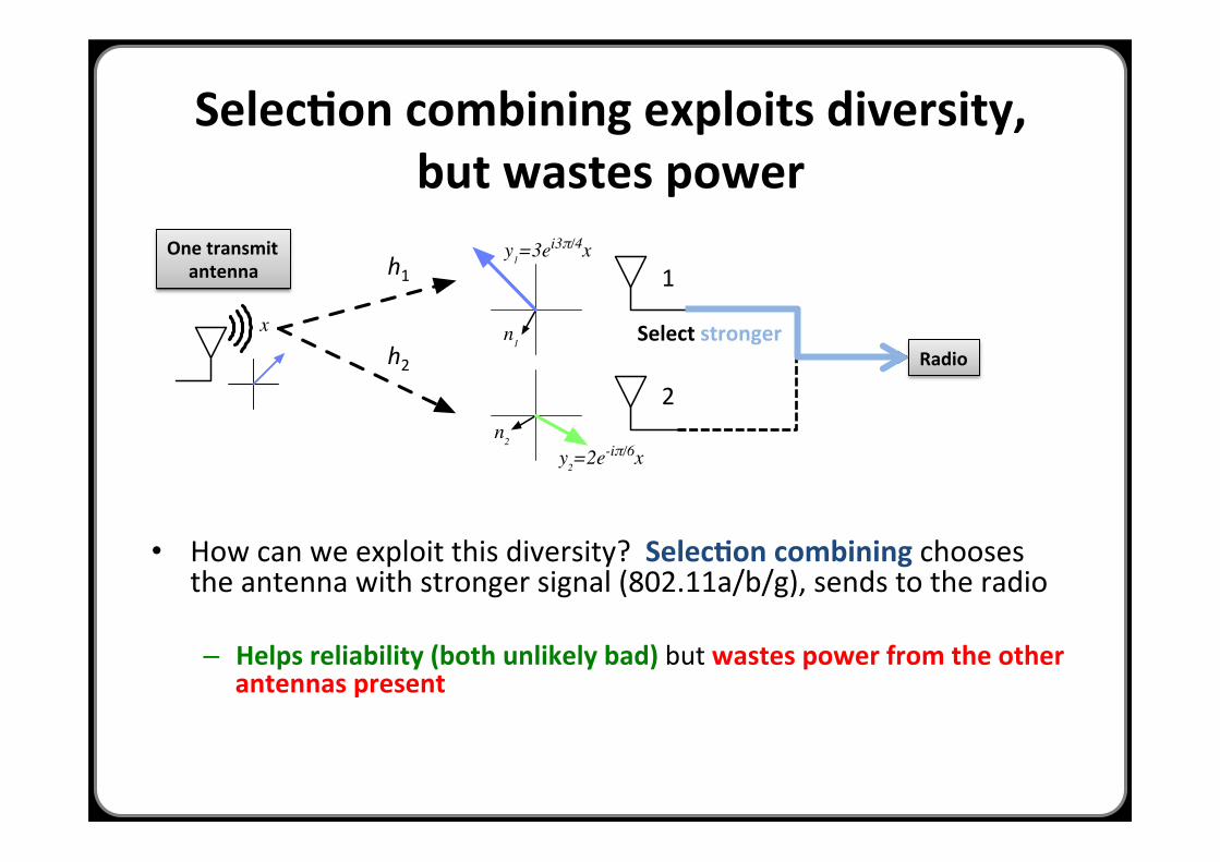
SelecAon combining exploits diversity, but wastes power
• How can we exploit this diversity? SelecAon combining chooses the antenna with stronger signal (802.11a/b/g), sends to the radio
– Helps reliability (both unlikely bad) but wastes power from the other antennas present
n2
y2=2e-iπ/6x
rotate, scale by 2/p
13
rotate, scale by 3/p
13
�
9/p
13
4/p
13
p13
x
n expected 1
y1=3ei3π/4x
n1
Figure 3: MRC operation on a sample channel. The channel gains are ~h = h3ei3⇡/4, 2e�i⇡/6i, with Gaussiannoise ~n = hn1, n2i of expected power 1. The antennas have respective SNRs of 9 and 4. To implement MRC,
the receiver multiplies the received signal ~y = ~hx + ~n by the unit vector ~h⇤/||~h||, where ~h⇤ denotes the complex
conjugate of ~h. This operation scales each antenna’s signal by its magnitude, and rotates the signals intothe same phase reference before adding them. (For graphical clarity, we depict the common phase vertically,rather than at 0). The resulting sum has magnitude
p13, and expected noise power 1 because the scaling is
normalized. Thus, by coherently combining received signals from di↵erent antennas, the MRC output hasthe expected SNR of 13. In systems with OFDM, MRC is performed separately for each subcarrier.
second node. This is known as a 1x2 system. Real systemsmay have more than two receive antennas, but two will suf-fice for our explanation. With this setup, each receive an-tenna receives a copy of the transmitted signal modified bythe channel between the transmitter and itself. The chan-nel gains hij are complex numbers that represent both theamplitude attenuation over the channel as well as the path-dependent phase shift (see Figure 3 for a graphical example).The receiver measures the channel gains based on trainingfields in the packet preamble. Note that the gains di↵er foreach subcarrier (in frequency-selective fading) as well as foreach antenna. The question now is how to combine the tworeceived signals to make best use of them.
We consider two diversity techniques to show the extremes.The simplest method is to use the antenna with the strongestsignal (hence the largest SNR) to receive the packet and ig-nore the others. We will call this method SEL, for selectioncombining. This is essentially what is done by 802.11a/g APswith multiple antennas. It helps with reliability, becauseboth signals are unlikely to be bad, but it wastes perfectlygood received power at the antennas that are not chosen.
The better method is to add the signals from the twoantennas together. However, this cannot be done by simplysuperimposing their signals, or we will have just recreatedthe e↵ects of multi-path fading. Rather, the signals shouldeach be delayed until they are in the same phase; then, thepower in the signals will combine coherently. To do this,the receiver needs a dedicated RF chain for each antenna toprocess the signals. This increases the hardware complexityand power consumption, but yields better performance.
As a twist in the above, the signals are also weighted bytheir SNRs. This gives less weight to a signal that has alarger fraction of noise, so that the e↵ects of the noise are notamplified. The result is maximal-ratio combining, or MRC.MRC is known to be optimal (it maximizes SIMO capacity),and produces an SNR that is the sum of the componentSNRs. Note that in frequency-selective fading, this processis performed di↵erently for each subcarrier according to itsspecific channel gains.
Figure 3 depicts MRC operation graphically for a 1x2channel. In this example, the two channel gains have magni-
-25
-20
-15
-10
-5
0
-20 -10 0 10 20
No
rma
lize
d p
ow
er
(dB
)
Subcarrier index
AC
B and SELAB (MRC)
ABC (MRC)
Figure 4: Frequency-selective fading over testbedlinks: the figure shows, for an example 5.2 GHz link,the received power measured on each subcarrier forindividual antennas and under SEL and MRC diver-sity, normalized to the strongest subcarrier power.
tudes of 3 and 2. With expected noise power 1, these gainscorrespond to SNRs of 9 and 4, given that a signal’s power isthe square of its magnitude. The MRC receiver scales eachantenna’s signal by its magnitude, normalized to the total;delays the signals to a common phase reference; and thenadds them. The result has magnitude
p13, and the normal-
ized weighted sum of noise still has expected power 1. Thecombined signal thus has a resulting sum SNR of 13.
As an example of how MRC and SEL work in 802.11, con-sider Figure 4. This figure shows the wireless signal strengthof each subcarrier using three antennas for a real 802.11n linkin our indoor wireless testbed. The subcarrier strengths aremeasured in decibels normalized to the strongest subcarrierstrength. This figure gives a much more detailed view thanmetrics such as the RSSI (Received Signal Strength Indi-cation) for a link, which gives only the sum of the signalstrength over all subcarriers.
For each antenna labeled A, B, or C, the signal variesover the channel, changing gradually from one subcarrier
One transmit antenna
Radio
Figure 1: A graphical view of the OFDM encoding process for the 18 Mbps rate (QPSK, 3/4) of 802.11a.The data bits (0) are encoded by a rate-1/2 convolutional code (1) and then optionally punctured by droppingcertain bits for higher coding rates (here, 3/4) that send fewer redundant bits (2). The remaining bits are in-terleaved (3) to spread the redundancy across subcarriers and protect against frequency-selective fades. Thesebits are grouped into symbols (4) based on the modulation (QPSK encodes 2 bits per symbol), modulated (5),and finally mapped onto the di↵erent subcarriers to form an OFDM symbol (6).
h11
h12
h11
h12y = x2
Tx Rx
y = xx
1
(a) Receive diversity
h11
h21
h11 h21
Tx Rx
x
x
( + ) xy =
y
(b) Transmit diversity
x1
x2
h11
h12h21
h22
h11x1 h21x2
h12x1 h22x2y2 = +
Tx Rx
y = 1 +
(c) Spatial multiplexing
Figure 2: Using some of the transmit/receive antennas in an example 2x2 system to exploit diversity andmultiplexing gain. xi and yi represent transmitted and received signals. The channel gain hij is a complexnumber indicating a signal’s attenuated amplitude and phase shift over the channel between the ith transmitantenna and the jth receive antenna. The received signals yi will additionally include thermal RF noise.
modulation sending more bits per symbol and being usedwhen there is a higher SNR. There are minor di↵erences be-tween 802.11a/g and 802.11n. In 802.11a/g there are 48 datasubcarriers, 4 pilot tones for control, and 6 unused guardsubcarriers at each edge of the channel. In 802.11n, thereare only 4 guard subcarriers at each edge of the channel, andtwo adjacent 20 MHz channels can be merged into a single40 MHz channel.
The beauty of OFDM is that it divides the channel in away that is both computationally and spectrally e�cient.High aggregate data rates can be achieved, while the en-coding and decoding on di↵erent subcarriers can use sharedhardware components. More relevant to our point here, how-ever, is that OFDM transforms a single large channel intomany relatively independently faded channels. This is be-cause multi-path fading is frequency selective, so the di↵er-ent subcarriers will experience di↵erent fades. Some adja-cent subcarriers may be faded in a similar way, but the fadingfor more distant subcarriers is often uncorrelated. Dividingthe channel also increases the symbol time per channel, sincemany slow symbols will be sent in parallel instead of manyfast symbols in sequence. This adds time diversity becausethe channel is more likely to average out fades over a longerperiod of time.
802.11 makes use of the frequency diversity provided byOFDM by coding across the data carried on the subcarriers.This uses a fraction of them for redundant information thatcan later be used to correct errors that occur when fadingreduces the SNR on some of the subcarriers. First, a con-
volutional code of rate 1/2 adds redundant information. Itis then punctured [3] by removing bits as needed to supportcoding rates of 2/3 and 3/4, plus 5/6 for 802.11n. At a rateof 3/4, for example, a quarter of the data on the subcarriersis redundant. An alternative LDPC (Low-Density Parity-Check) code with slightly better performance can also beused for 802.11n. Figure 1 presents a pictorial overview ofthe OFDM encoding process.
The net e↵ect of OFDM plus coding is to provide consis-tently good 802.11 performance despite significant variabil-ity in the wireless signal due to multi-path fading.
3. SPATIAL DIVERSITYIn this section we look at spatial diversity techniques that
can be applied at the receiver and at the transmitter. Addingmultiple antennas to an 802.11n receiver or transmitter pro-vides a new set of independently faded paths, even if theantennas are separated by only a few centimeters. Thisadds spatial diversity to the system, which can be exploitedto improve resilience to fades. There is also a power gainfrom multiple receive antennas because, everything else be-ing equal, two receive antennas will receive twice the signal.These factors combine to improve performance at a givendistance, and hence increase range.
3.1 Receive Diversity TechniquesConsider the arrangement in Figure 2(a). One transmit
antenna at a node is sending to two receive antennas at a
1
2
h1
h2 Select stronger
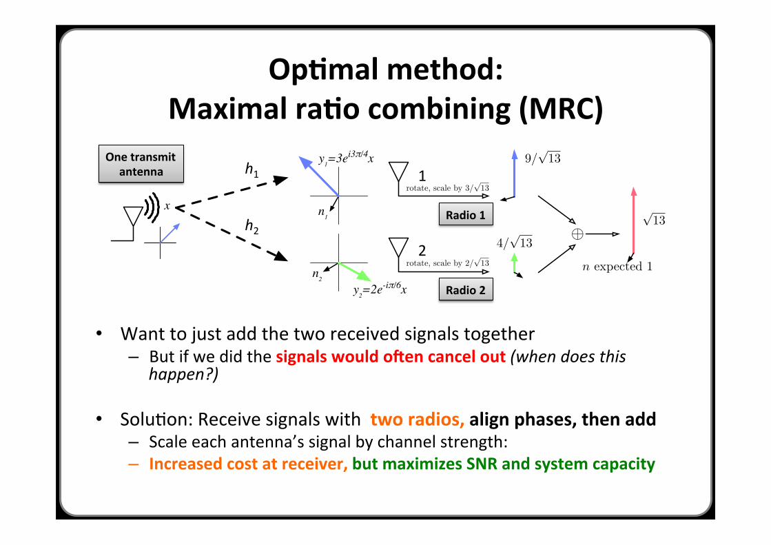
OpAmal method: Maximal raAo combining (MRC)
• Want to just add the two received signals together – But if we did the signals would oZen cancel out (when does this
happen?)
• SoluHon: Receive signals with two radios, align phases, then add – Scale each antenna’s signal by channel strength: – Increased cost at receiver, but maximizes SNR and system capacity
n2
y2=2e-iπ/6x
rotate, scale by 2/p
13
rotate, scale by 3/p
13
�
9/p
13
4/p
13
p13
x
n expected 1
y1=3ei3π/4x
n1
Figure 3: MRC operation on a sample channel. The channel gains are ~h = h3ei3⇡/4, 2e�i⇡/6i, with Gaussiannoise ~n = hn1, n2i of expected power 1. The antennas have respective SNRs of 9 and 4. To implement MRC,
the receiver multiplies the received signal ~y = ~hx + ~n by the unit vector ~h⇤/||~h||, where ~h⇤ denotes the complex
conjugate of ~h. This operation scales each antenna’s signal by its magnitude, and rotates the signals intothe same phase reference before adding them. (For graphical clarity, we depict the common phase vertically,rather than at 0). The resulting sum has magnitude
p13, and expected noise power 1 because the scaling is
normalized. Thus, by coherently combining received signals from di↵erent antennas, the MRC output hasthe expected SNR of 13. In systems with OFDM, MRC is performed separately for each subcarrier.
second node. This is known as a 1x2 system. Real systemsmay have more than two receive antennas, but two will suf-fice for our explanation. With this setup, each receive an-tenna receives a copy of the transmitted signal modified bythe channel between the transmitter and itself. The chan-nel gains hij are complex numbers that represent both theamplitude attenuation over the channel as well as the path-dependent phase shift (see Figure 3 for a graphical example).The receiver measures the channel gains based on trainingfields in the packet preamble. Note that the gains di↵er foreach subcarrier (in frequency-selective fading) as well as foreach antenna. The question now is how to combine the tworeceived signals to make best use of them.
We consider two diversity techniques to show the extremes.The simplest method is to use the antenna with the strongestsignal (hence the largest SNR) to receive the packet and ig-nore the others. We will call this method SEL, for selectioncombining. This is essentially what is done by 802.11a/g APswith multiple antennas. It helps with reliability, becauseboth signals are unlikely to be bad, but it wastes perfectlygood received power at the antennas that are not chosen.
The better method is to add the signals from the twoantennas together. However, this cannot be done by simplysuperimposing their signals, or we will have just recreatedthe e↵ects of multi-path fading. Rather, the signals shouldeach be delayed until they are in the same phase; then, thepower in the signals will combine coherently. To do this,the receiver needs a dedicated RF chain for each antenna toprocess the signals. This increases the hardware complexityand power consumption, but yields better performance.
As a twist in the above, the signals are also weighted bytheir SNRs. This gives less weight to a signal that has alarger fraction of noise, so that the e↵ects of the noise are notamplified. The result is maximal-ratio combining, or MRC.MRC is known to be optimal (it maximizes SIMO capacity),and produces an SNR that is the sum of the componentSNRs. Note that in frequency-selective fading, this processis performed di↵erently for each subcarrier according to itsspecific channel gains.
Figure 3 depicts MRC operation graphically for a 1x2channel. In this example, the two channel gains have magni-
-25
-20
-15
-10
-5
0
-20 -10 0 10 20
No
rma
lize
d p
ow
er
(dB
)
Subcarrier index
AC
B and SELAB (MRC)
ABC (MRC)
Figure 4: Frequency-selective fading over testbedlinks: the figure shows, for an example 5.2 GHz link,the received power measured on each subcarrier forindividual antennas and under SEL and MRC diver-sity, normalized to the strongest subcarrier power.
tudes of 3 and 2. With expected noise power 1, these gainscorrespond to SNRs of 9 and 4, given that a signal’s power isthe square of its magnitude. The MRC receiver scales eachantenna’s signal by its magnitude, normalized to the total;delays the signals to a common phase reference; and thenadds them. The result has magnitude
p13, and the normal-
ized weighted sum of noise still has expected power 1. Thecombined signal thus has a resulting sum SNR of 13.
As an example of how MRC and SEL work in 802.11, con-sider Figure 4. This figure shows the wireless signal strengthof each subcarrier using three antennas for a real 802.11n linkin our indoor wireless testbed. The subcarrier strengths aremeasured in decibels normalized to the strongest subcarrierstrength. This figure gives a much more detailed view thanmetrics such as the RSSI (Received Signal Strength Indi-cation) for a link, which gives only the sum of the signalstrength over all subcarriers.
For each antenna labeled A, B, or C, the signal variesover the channel, changing gradually from one subcarrier
One transmit antenna
Figure 1: A graphical view of the OFDM encoding process for the 18 Mbps rate (QPSK, 3/4) of 802.11a.The data bits (0) are encoded by a rate-1/2 convolutional code (1) and then optionally punctured by droppingcertain bits for higher coding rates (here, 3/4) that send fewer redundant bits (2). The remaining bits are in-terleaved (3) to spread the redundancy across subcarriers and protect against frequency-selective fades. Thesebits are grouped into symbols (4) based on the modulation (QPSK encodes 2 bits per symbol), modulated (5),and finally mapped onto the di↵erent subcarriers to form an OFDM symbol (6).
h11
h12
h11
h12y = x2
Tx Rx
y = xx
1
(a) Receive diversity
h11
h21
h11 h21
Tx Rx
x
x
( + ) xy =
y
(b) Transmit diversity
x1
x2
h11
h12h21
h22
h11x1 h21x2
h12x1 h22x2y2 = +
Tx Rx
y = 1 +
(c) Spatial multiplexing
Figure 2: Using some of the transmit/receive antennas in an example 2x2 system to exploit diversity andmultiplexing gain. xi and yi represent transmitted and received signals. The channel gain hij is a complexnumber indicating a signal’s attenuated amplitude and phase shift over the channel between the ith transmitantenna and the jth receive antenna. The received signals yi will additionally include thermal RF noise.
modulation sending more bits per symbol and being usedwhen there is a higher SNR. There are minor di↵erences be-tween 802.11a/g and 802.11n. In 802.11a/g there are 48 datasubcarriers, 4 pilot tones for control, and 6 unused guardsubcarriers at each edge of the channel. In 802.11n, thereare only 4 guard subcarriers at each edge of the channel, andtwo adjacent 20 MHz channels can be merged into a single40 MHz channel.
The beauty of OFDM is that it divides the channel in away that is both computationally and spectrally e�cient.High aggregate data rates can be achieved, while the en-coding and decoding on di↵erent subcarriers can use sharedhardware components. More relevant to our point here, how-ever, is that OFDM transforms a single large channel intomany relatively independently faded channels. This is be-cause multi-path fading is frequency selective, so the di↵er-ent subcarriers will experience di↵erent fades. Some adja-cent subcarriers may be faded in a similar way, but the fadingfor more distant subcarriers is often uncorrelated. Dividingthe channel also increases the symbol time per channel, sincemany slow symbols will be sent in parallel instead of manyfast symbols in sequence. This adds time diversity becausethe channel is more likely to average out fades over a longerperiod of time.
802.11 makes use of the frequency diversity provided byOFDM by coding across the data carried on the subcarriers.This uses a fraction of them for redundant information thatcan later be used to correct errors that occur when fadingreduces the SNR on some of the subcarriers. First, a con-
volutional code of rate 1/2 adds redundant information. Itis then punctured [3] by removing bits as needed to supportcoding rates of 2/3 and 3/4, plus 5/6 for 802.11n. At a rateof 3/4, for example, a quarter of the data on the subcarriersis redundant. An alternative LDPC (Low-Density Parity-Check) code with slightly better performance can also beused for 802.11n. Figure 1 presents a pictorial overview ofthe OFDM encoding process.
The net e↵ect of OFDM plus coding is to provide consis-tently good 802.11 performance despite significant variabil-ity in the wireless signal due to multi-path fading.
3. SPATIAL DIVERSITYIn this section we look at spatial diversity techniques that
can be applied at the receiver and at the transmitter. Addingmultiple antennas to an 802.11n receiver or transmitter pro-vides a new set of independently faded paths, even if theantennas are separated by only a few centimeters. Thisadds spatial diversity to the system, which can be exploitedto improve resilience to fades. There is also a power gainfrom multiple receive antennas because, everything else be-ing equal, two receive antennas will receive twice the signal.These factors combine to improve performance at a givendistance, and hence increase range.
3.1 Receive Diversity TechniquesConsider the arrangement in Figure 2(a). One transmit
antenna at a node is sending to two receive antennas at a
1
2
h1
h2 Radio 1
Radio 2
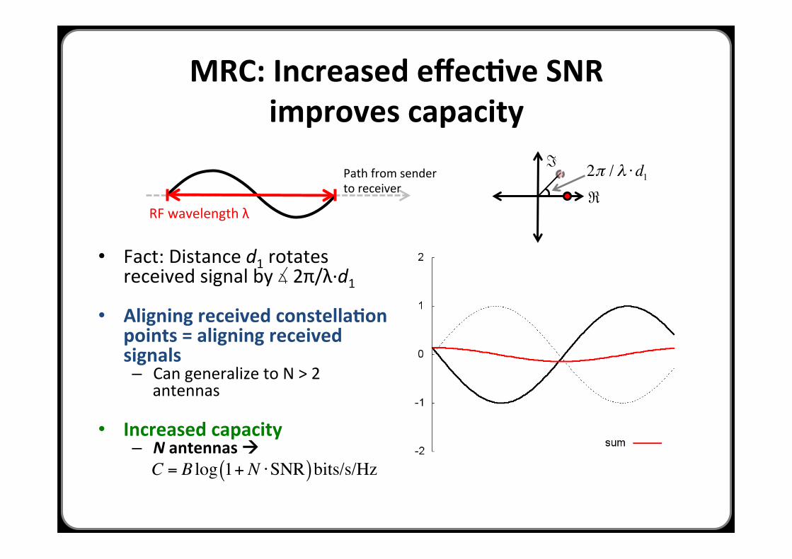
MRC: Increased effecAve SNR improves capacity
• Fact: Distance d1 rotates received signal by ∡ 2π/λ·∙d1
• Aligning received constellaAon points = aligning received signals – Can generalize to N > 2
antennas
• Increased capacity – N antennas à
RF wavelength λ
Path from sender to receiver
ℑ
ℜ
2π / λ ⋅d1
C = B log 1+ N ⋅SNR( )bits/s/Hz
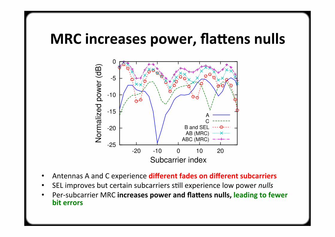
MRC increases power, fla^ens nulls
• Antennas A and C experience different fades on different subcarriers • SEL improves but certain subcarriers sHll experience low power nulls • Per-‐subcarrier MRC increases power and fla^ens nulls, leading to fewer
bit errors
n2
y2=2e-iπ/6x
rotate, scale by 2/p
13
rotate, scale by 3/p
13
�
9/p
13
4/p
13
p13
x
n expected 1
y1=3ei3π/4x
n1
Figure 3: MRC operation on a sample channel. The channel gains are ~h = h3ei3⇡/4, 2e�i⇡/6i, with Gaussiannoise ~n = hn1, n2i of expected power 1. The antennas have respective SNRs of 9 and 4. To implement MRC,
the receiver multiplies the received signal ~y = ~hx + ~n by the unit vector ~h⇤/||~h||, where ~h⇤ denotes the complex
conjugate of ~h. This operation scales each antenna’s signal by its magnitude, and rotates the signals intothe same phase reference before adding them. (For graphical clarity, we depict the common phase vertically,rather than at 0). The resulting sum has magnitude
p13, and expected noise power 1 because the scaling is
normalized. Thus, by coherently combining received signals from di↵erent antennas, the MRC output hasthe expected SNR of 13. In systems with OFDM, MRC is performed separately for each subcarrier.
second node. This is known as a 1x2 system. Real systemsmay have more than two receive antennas, but two will suf-fice for our explanation. With this setup, each receive an-tenna receives a copy of the transmitted signal modified bythe channel between the transmitter and itself. The chan-nel gains hij are complex numbers that represent both theamplitude attenuation over the channel as well as the path-dependent phase shift (see Figure 3 for a graphical example).The receiver measures the channel gains based on trainingfields in the packet preamble. Note that the gains di↵er foreach subcarrier (in frequency-selective fading) as well as foreach antenna. The question now is how to combine the tworeceived signals to make best use of them.
We consider two diversity techniques to show the extremes.The simplest method is to use the antenna with the strongestsignal (hence the largest SNR) to receive the packet and ig-nore the others. We will call this method SEL, for selectioncombining. This is essentially what is done by 802.11a/g APswith multiple antennas. It helps with reliability, becauseboth signals are unlikely to be bad, but it wastes perfectlygood received power at the antennas that are not chosen.
The better method is to add the signals from the twoantennas together. However, this cannot be done by simplysuperimposing their signals, or we will have just recreatedthe e↵ects of multi-path fading. Rather, the signals shouldeach be delayed until they are in the same phase; then, thepower in the signals will combine coherently. To do this,the receiver needs a dedicated RF chain for each antenna toprocess the signals. This increases the hardware complexityand power consumption, but yields better performance.
As a twist in the above, the signals are also weighted bytheir SNRs. This gives less weight to a signal that has alarger fraction of noise, so that the e↵ects of the noise are notamplified. The result is maximal-ratio combining, or MRC.MRC is known to be optimal (it maximizes SIMO capacity),and produces an SNR that is the sum of the componentSNRs. Note that in frequency-selective fading, this processis performed di↵erently for each subcarrier according to itsspecific channel gains.
Figure 3 depicts MRC operation graphically for a 1x2channel. In this example, the two channel gains have magni-
-25
-20
-15
-10
-5
0
-20 -10 0 10 20
No
rma
lize
d p
ow
er
(dB
)
Subcarrier index
AC
B and SELAB (MRC)
ABC (MRC)
Figure 4: Frequency-selective fading over testbedlinks: the figure shows, for an example 5.2 GHz link,the received power measured on each subcarrier forindividual antennas and under SEL and MRC diver-sity, normalized to the strongest subcarrier power.
tudes of 3 and 2. With expected noise power 1, these gainscorrespond to SNRs of 9 and 4, given that a signal’s power isthe square of its magnitude. The MRC receiver scales eachantenna’s signal by its magnitude, normalized to the total;delays the signals to a common phase reference; and thenadds them. The result has magnitude
p13, and the normal-
ized weighted sum of noise still has expected power 1. Thecombined signal thus has a resulting sum SNR of 13.
As an example of how MRC and SEL work in 802.11, con-sider Figure 4. This figure shows the wireless signal strengthof each subcarrier using three antennas for a real 802.11n linkin our indoor wireless testbed. The subcarrier strengths aremeasured in decibels normalized to the strongest subcarrierstrength. This figure gives a much more detailed view thanmetrics such as the RSSI (Received Signal Strength Indi-cation) for a link, which gives only the sum of the signalstrength over all subcarriers.
For each antenna labeled A, B, or C, the signal variesover the channel, changing gradually from one subcarrier
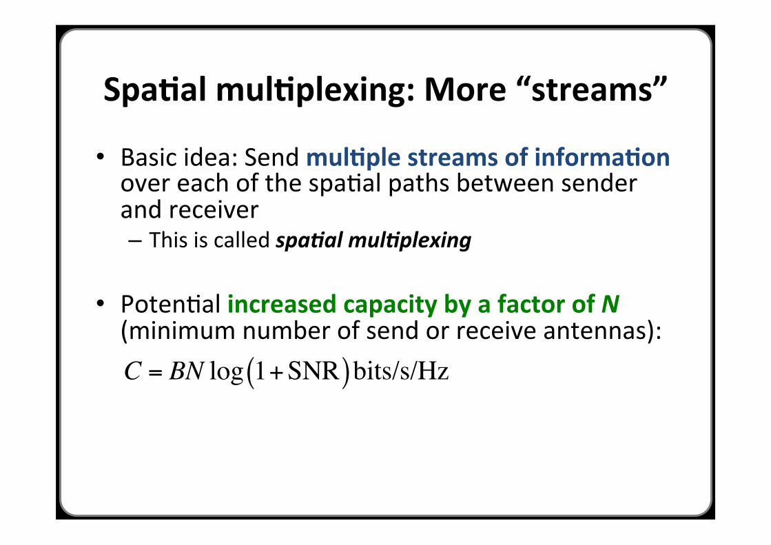
SpaAal mulAplexing: More “streams”
• Basic idea: Send mulAple streams of informaAon over each of the spaHal paths between sender and receiver – This is called spa(al mul(plexing
• PotenHal increased capacity by a factor of N (minimum number of send or receive antennas): C = BN log 1+SNR( )bits/s/Hz
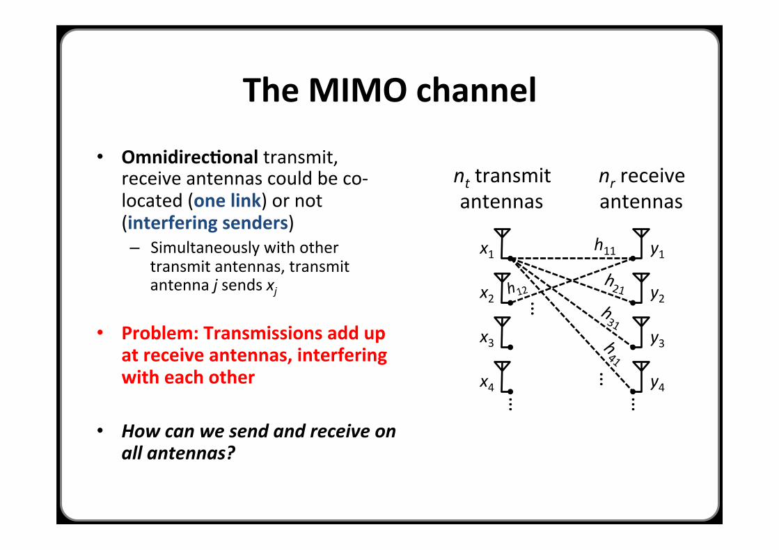
• OmnidirecAonal transmit, receive antennas could be co-‐located (one link) or not (interfering senders) – Simultaneously with other
transmit antennas, transmit antenna j sends xj
• Problem: Transmissions add up at receive antennas, interfering with each other
• How can we send and receive on all antennas?
The MIMO channel
h11
nt transmit antennas
nr receive antennas
h21 h12 …
…
…
…
x1
x2
x3
x4
y3
y4
y2
y1
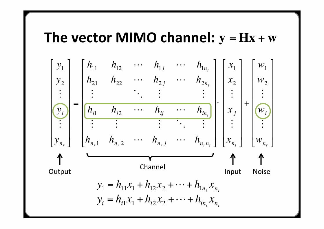
The vector MIMO channel:
€
y =Hx +w
€
y1y2yiynr
"
#
$ $ $ $ $ $ $
%
&
' ' ' ' ' ' '
=
h11 h12 h1 j h1nth21 h22 h2 j h2nt hi1 hi2 hij hint hnr1 hnr 2 hnr j hnr nt
"
#
$ $ $ $ $ $ $
%
&
' ' ' ' ' ' '
⋅
x1x2x j
xnt
"
#
$ $ $ $ $ $ $
%
&
' ' ' ' ' ' '
+
w1w2
wi
wnr
"
#
$ $ $ $ $ $ $
%
&
' ' ' ' ' ' '
Output Channel Input
€
yi = hi1x1 + hi2x2 ++ hint xnt
Noise
€
y1 = h11x1 + h12x2 ++ h1nt xnt
The vector MIMO channel:
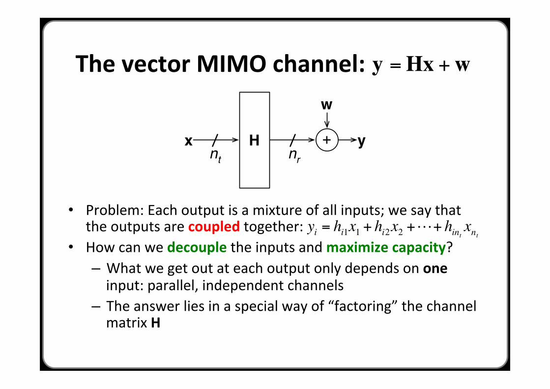
• Problem: Each output is a mixture of all inputs; we say that the outputs are coupled together:
• How can we decouple the inputs and maximize capacity? – What we get out at each output only depends on one input: parallel, independent channels
– The answer lies in a special way of “factoring” the channel matrix H
x H +
w
ynt nr
€
yi = hi1x1 + hi2x2 ++ hint xnt
€
y =Hx +w
The singular value decomposiAon (SVD)
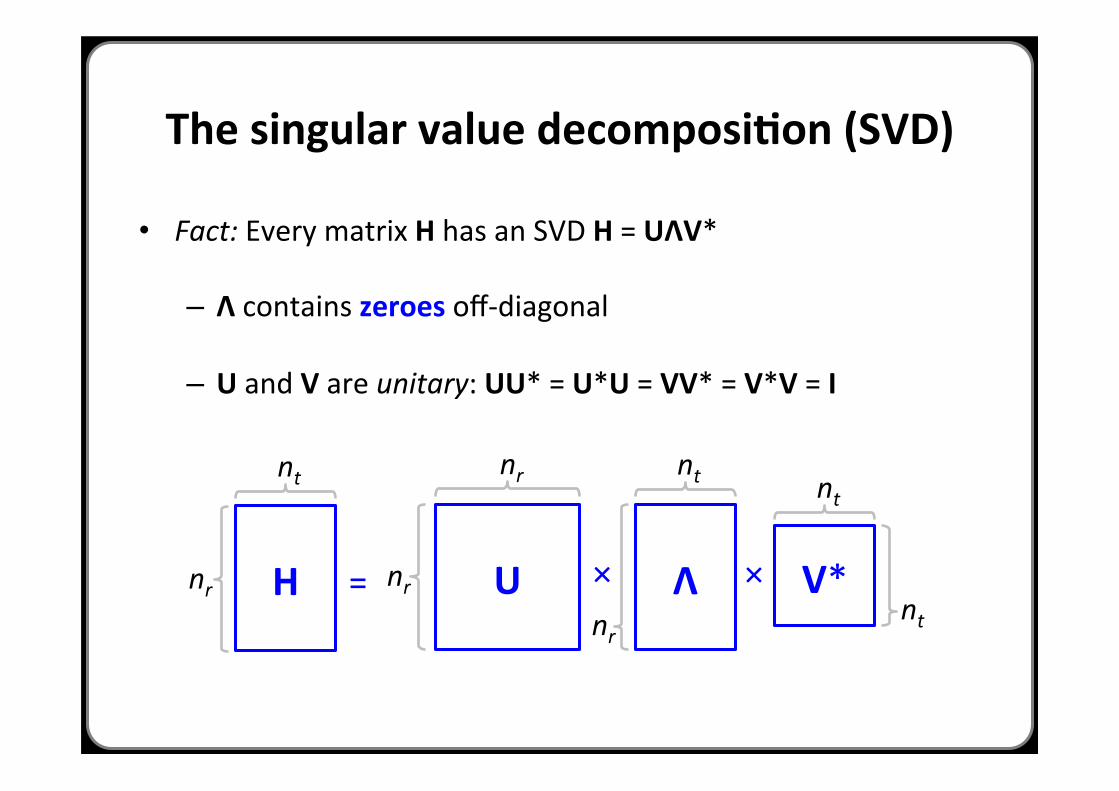
• Fact: Every matrix H has an SVD H = UΛV*
– Λ contains zeroes off-‐diagonal
– U and V are unitary: UU* = U*U = VV* = V*V = I
H =
nt
nr Λ
nt
nr V* ×
nt
nt U ×
nr
nr
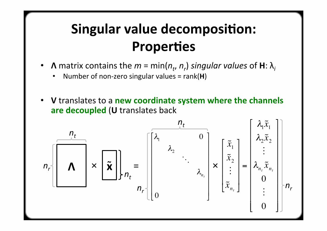
Singular value decomposiAon: ProperAes
• Λ matrix contains the m = min(nt, nr) singular values of H: λi • Number of non-‐zero singular values = rank(H)
• V translates to a new coordinate system where the channels are decoupled (U translates back
€
λ1 0λ2
λnt
0
#
$
% % % % % % %
&
'
( ( ( ( ( ( (
Λ
nt
nr =
nt
nr
€
˜ x 1˜ x 2
˜ x nt
"
#
$ $ $ $
%
&
' ' ' '
=
λ1 ˜ x 1λ2 ˜ x 2
λnt˜ x nt
00
"
#
$ $ $ $ $ $ $ $ $
%
&
' ' ' ' ' ' ' ' '
x × nt
~ ×
nr
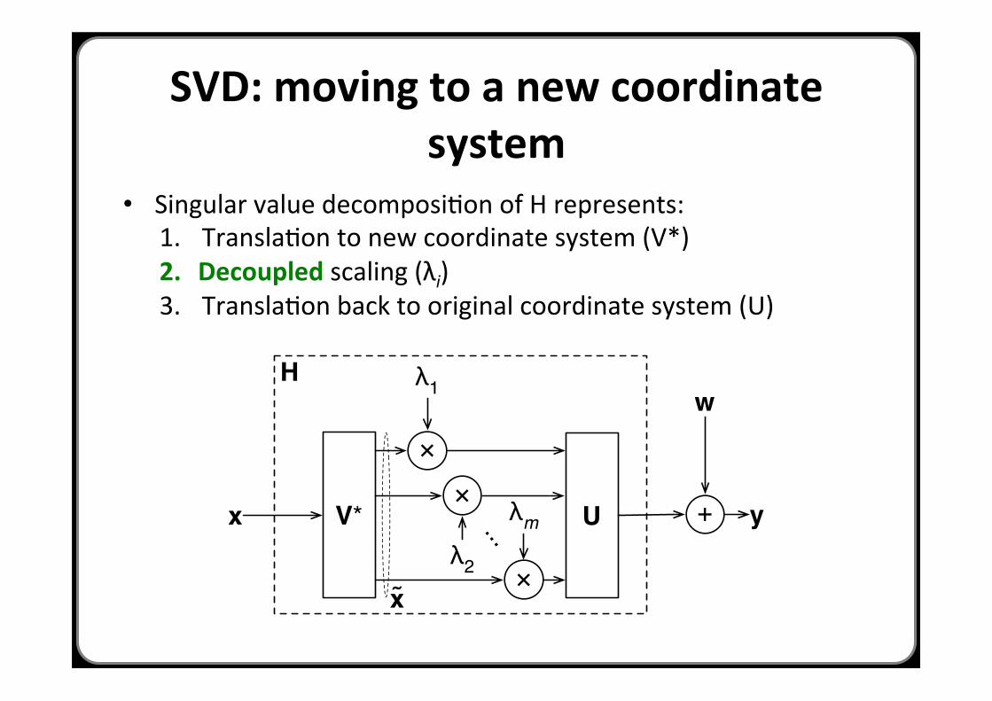
SVD: moving to a new coordinate system
• Singular value decomposiHon of H represents: 1. TranslaHon to new coordinate system (V*) 2. Decoupled scaling (λi) 3. TranslaHon back to original coordinate system (U)
x V* +
w
y
×
×
×
λ1
λ2
λm...U
H
x
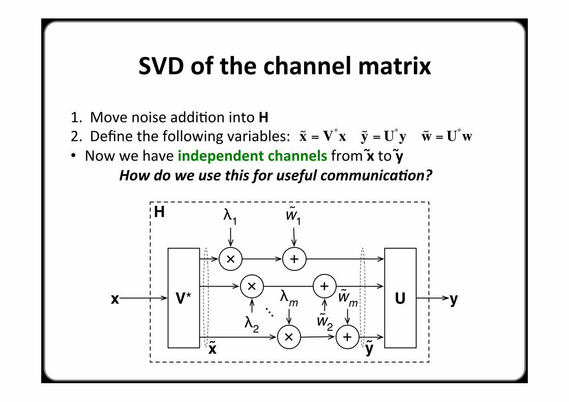
SVD of the channel matrix
1. Move noise addiHon into H 2. Define the following variables: • Now we have independent channels from x to y How do we use this for useful communica(on?
x V* y
×
×
×
λ1
λ2
λm...U
+
+
+
w1
w2
wm
x y
H€
˜ x = V*x ˜ y = U*y ˜ w = U*w~ ~
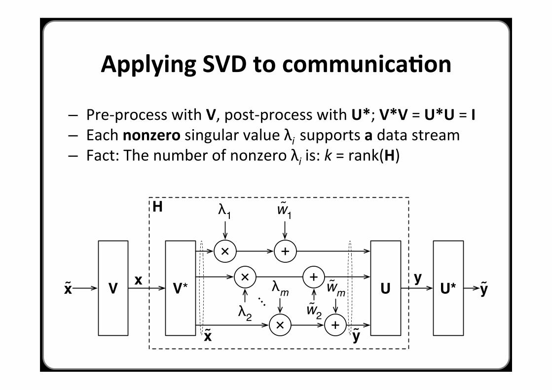
Applying SVD to communicaAon
x V*y
×
×
×
λ1
λ2
λm...U
+
+
+
w1
w2
wm
x y
H
Vx U* y
– Pre-‐process with V, post-‐process with U*; V*V = U*U = I – Each nonzero singular value λi supports a data stream – Fact: The number of nonzero λi is: k = rank(H)
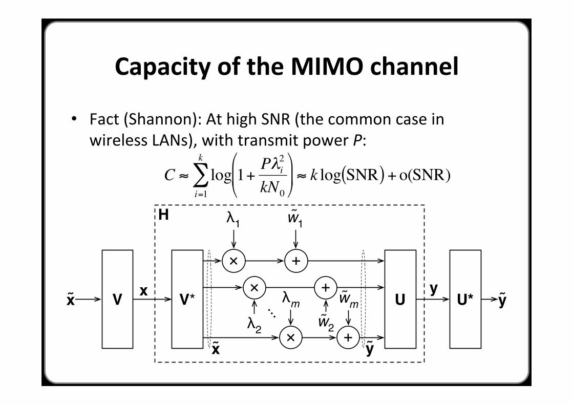
Capacity of the MIMO channel
x V*y
×
×
×
λ1
λ2
λm...U
+
+
+
w1
w2
wm
x y
H
Vx U* y
• Fact (Shannon): At high SNR (the common case in wireless LANs), with transmit power P:
€
C ≈ log 1+Pλi
2
kN0
$
% &
'
( )
i=1
k
∑ ≈ k log SNR( ) + o(SNR)
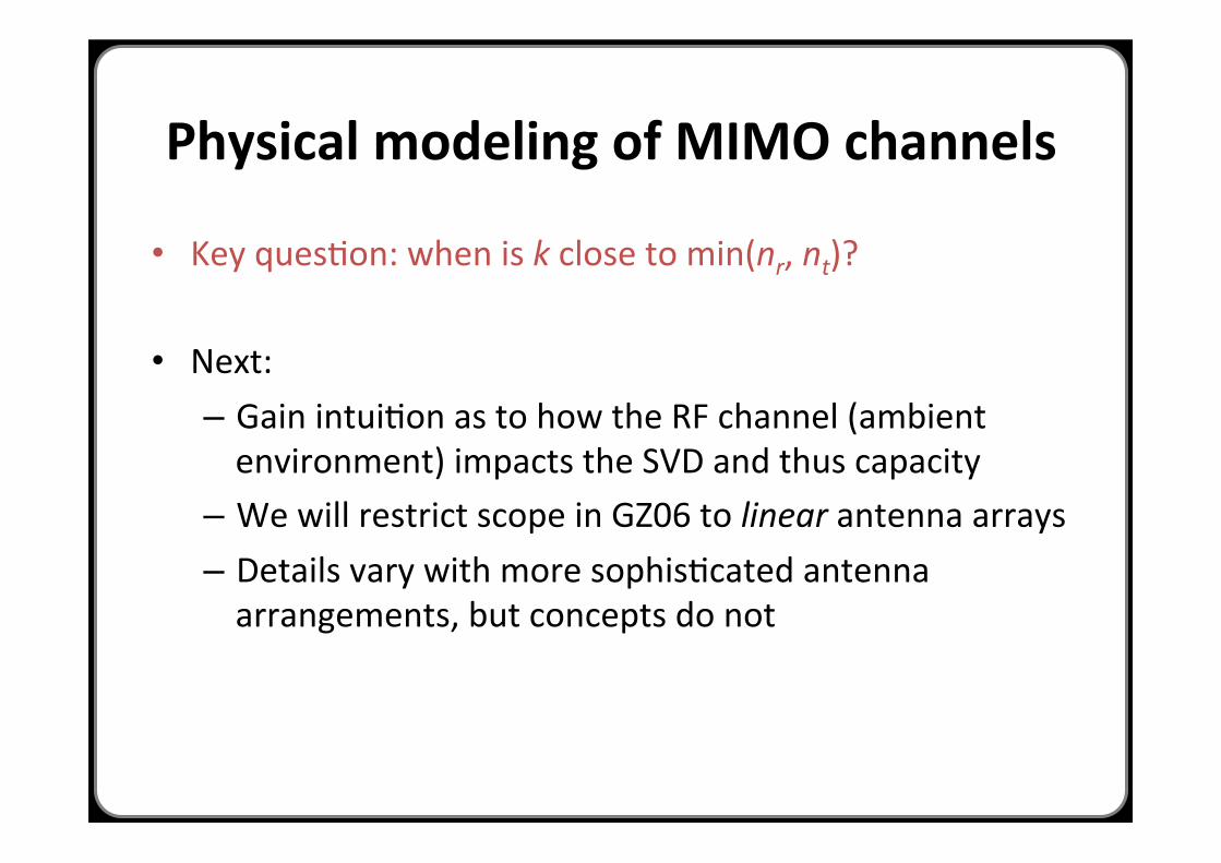
Physical modeling of MIMO channels
• Key quesHon: when is k close to min(nr, nt)?
• Next: – Gain intuiHon as to how the RF channel (ambient environment) impacts the SVD and thus capacity
– We will restrict scope in GZ06 to linear antenna arrays – Details vary with more sophisHcated antenna arrangements, but concepts do not
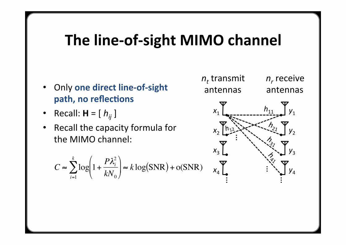
• Only one direct line-‐of-‐sight path, no reflecAons
• Recall: H = [ hij ] • Recall the capacity formula for
the MIMO channel:
The line-‐of-‐sight MIMO channel
h11
nt transmit antennas
nr receive antennas
h21 h12 …
…
…
…
x1
x2
x3
x4
y3
y4
y2
y1
€
C ≈ log 1+Pλi
2
kN0
$
% &
'
( )
i=1
k
∑ ≈ k log SNR( ) + o(SNR)
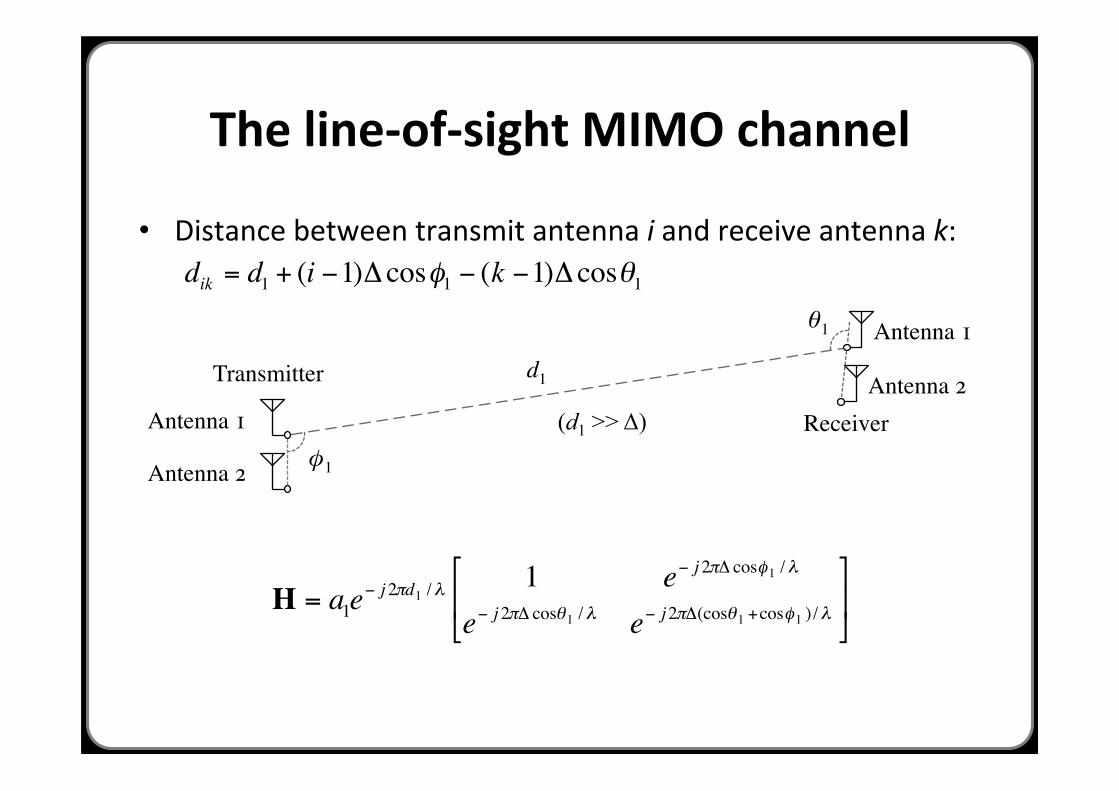
The line-‐of-‐sight MIMO channel
• Distance between transmit antenna i and receive antenna k:
d1
θ1
Transmitter
Receiver
Antenna 1
Antenna 2
φ1
Antenna 1
Antenna 2
€
dik = d1 + (i −1)Δ cosφ1 − (k −1)Δ cosθ1
€
H = a1e− j 2πd1 /λ
1 e− j 2πΔ cosφ1 /λ
e− j 2πΔ cosθ1 /λ e− j2πΔ(cosθ1 +cosφ1 ) /λ
(
) *
+
, -
(d1 >> Δ)
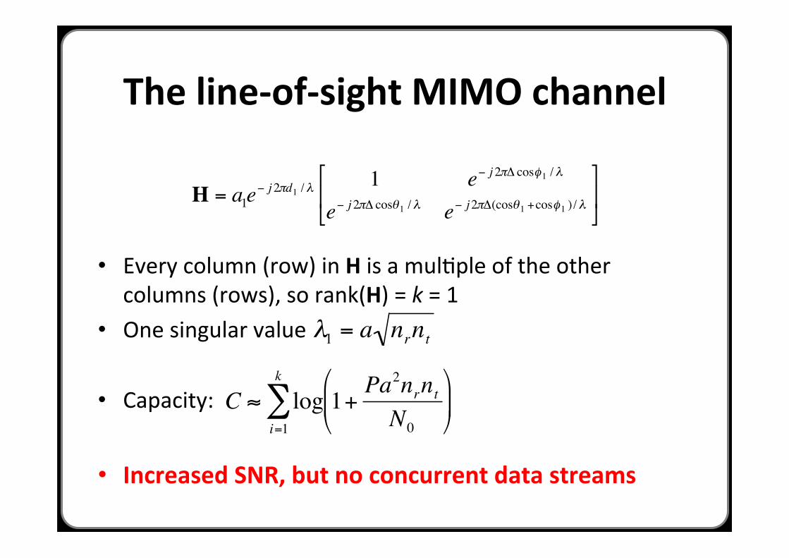
The line-‐of-‐sight MIMO channel
• Every column (row) in H is a mulHple of the other columns (rows), so rank(H) = k = 1
• One singular value
• Capacity:
• Increased SNR, but no concurrent data streams
€
C ≈ log 1+Pa2nrntN0
#
$ %
&
' (
i=1
k
∑€
λ1 = a nrnt€
H = a1e− j 2πd1 /λ
1 e− j 2πΔ cosφ1 /λ
e− j 2πΔ cosθ1 /λ e− j2πΔ(cosθ1 +cosφ1 ) /λ
(
) *
+
, -
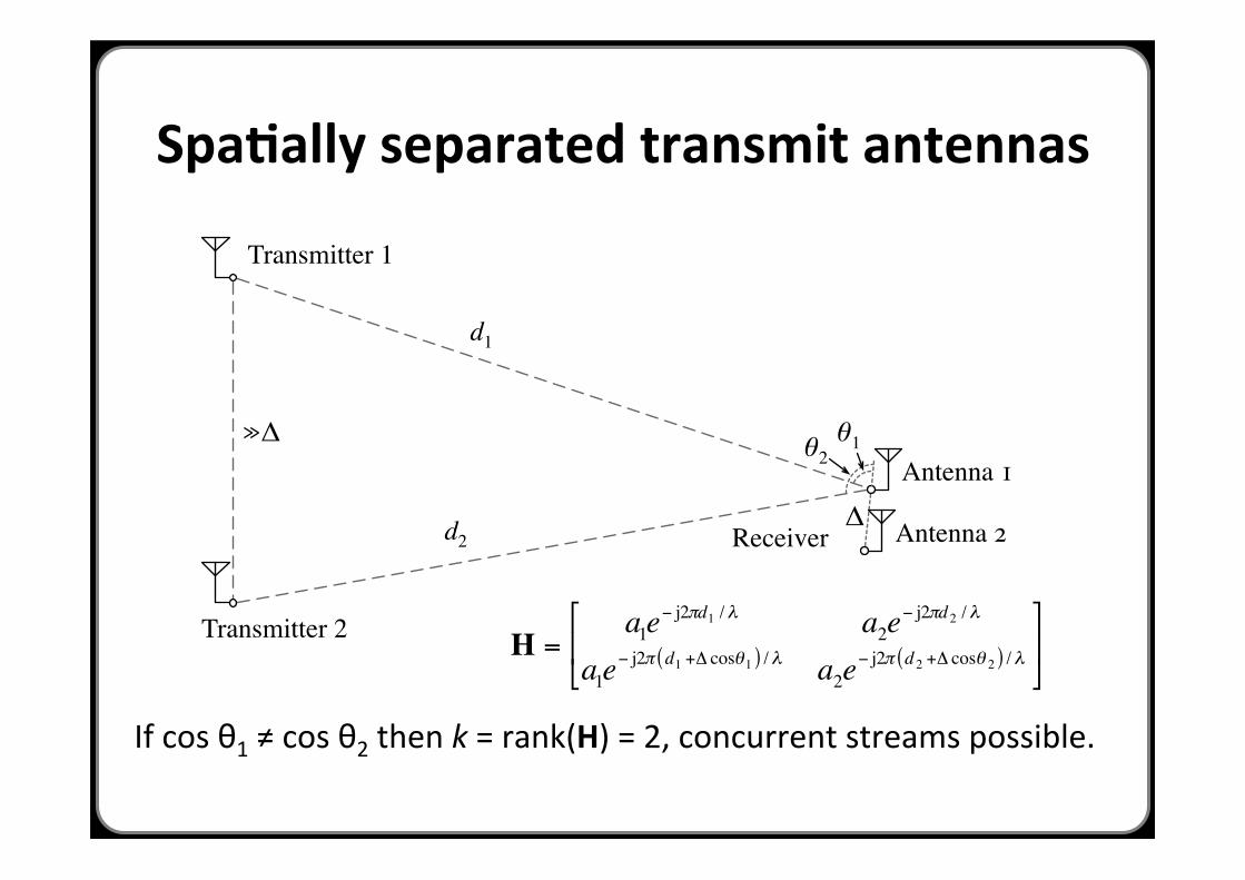
SpaAally separated transmit antennas
d1
Δ
θ1
Transmitter 2
Receiver
Antenna 1
Antenna 2
θ2
Transmitter 1
d2
≫Δ
€
H =a1e
− j2πd1 /λ a2e− j2πd2 /λ
a1e− j2π d1 +Δ cosθ1( ) /λ a2e
− j2π d 2 +Δ cosθ 2( ) /λ
'
( )
*
+ ,
If cos θ1 ≠ cos θ2 then k = rank(H) = 2, concurrent streams possible.

SpaAally separated receive antennas
d1TransmitterReceiver 1
Receiver 2
!2
Antenna 1
Antenna 2!1
d2≫!
€
H =a1e
− j2πd1 /λ a1e− j2π d1 +Δ cosφ1( ) /λ
a2e− j2πd2 /λ a2e
− j2π d2 +Δ cosφ 2( ) /λ
'
( )
*
+ ,
If cos ϕ1 ≠ cos ϕ2 then k = rank(H) = 2, concurrent streams possible.
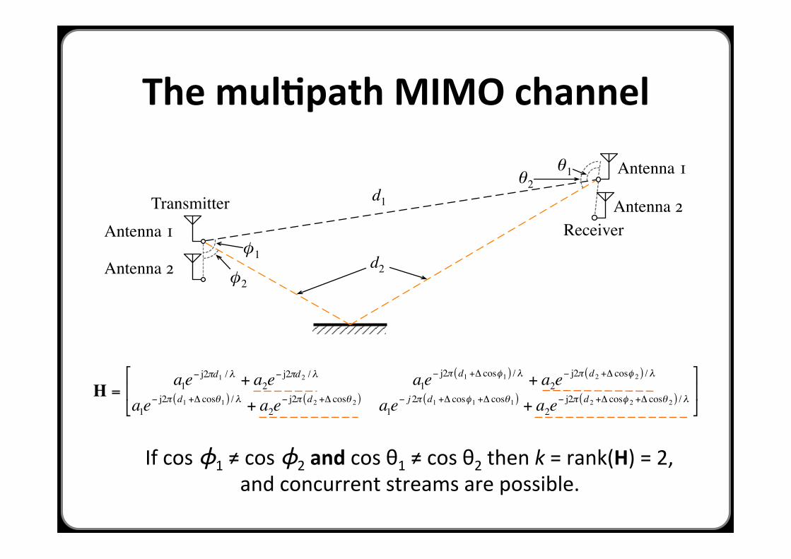
The mulApath MIMO channel
d1
θ1 Antenna 1
Antenna 2
φ1Antenna 1
Antenna 2 φ2
θ2
d2
ReceiverTransmitter
If cos ϕ1 ≠ cos ϕ2 and cos θ1 ≠ cos θ2 then k = rank(H) = 2, and concurrent streams are possible. €
H =a1e
− j2πd1 /λ + a2e− j2πd 2 /λ a1e
− j2π d1 +Δ cosφ1( ) /λ + a2e− j2π d2 +Δ cosφ 2( ) /λ
a1e− j2π d1 +Δ cosθ1( ) /λ + a2e
− j2π d2 +Δ cosθ 2( ) a1e− j 2π d1 +Δ cosφ1 +Δ cosθ1( ) + a2e
− j2π d2 +Δ cosφ 2 +Δ cosθ 2( ) /λ
(
) *
+
, -
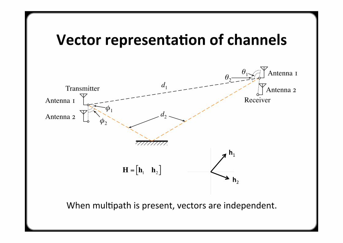
Vector representaAon of channels
d1
θ1 Antenna 1
Antenna 2
φ1Antenna 1
Antenna 2 φ2
θ2
d2
ReceiverTransmitter
When mulHpath is present, vectors are independent. €
H = h1 h2[ ]
h1
h2
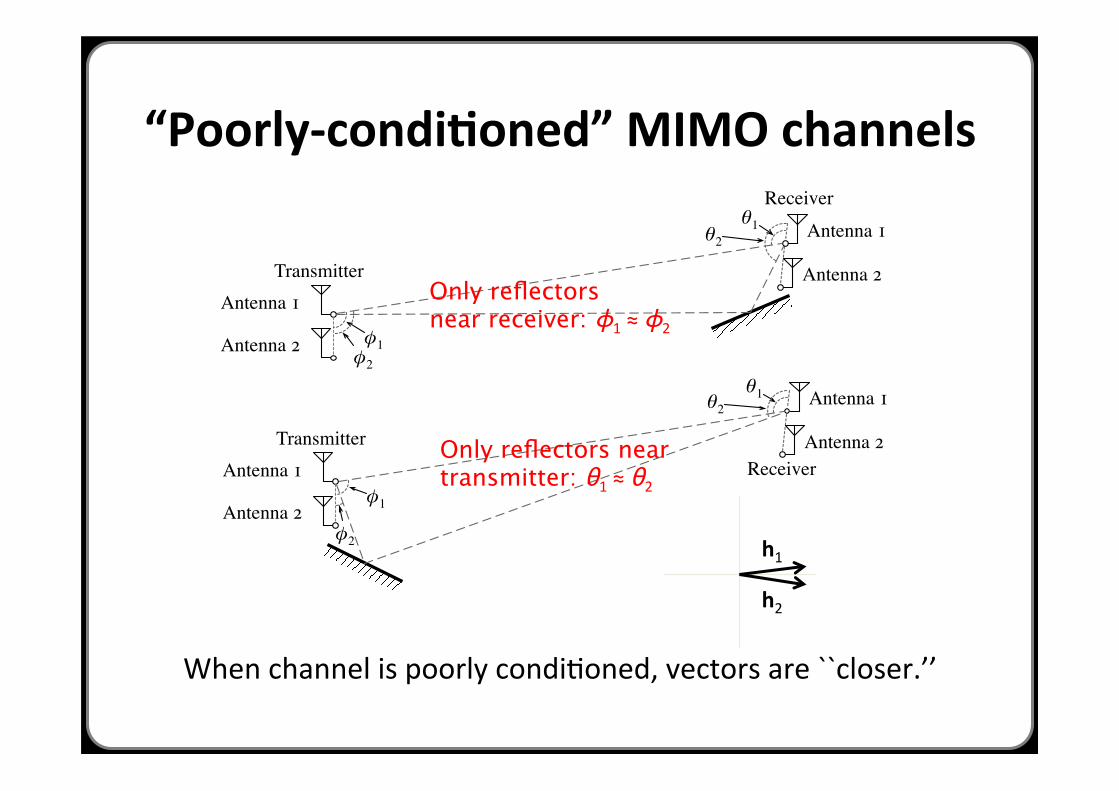
“Poorly-‐condiAoned” MIMO channels !1 Antenna 1
Antenna 2
"1
Antenna 1
Antenna 2 "2
!2
Receiver
TransmitterOnly reflectors near receiver: ϕ1 ≈ ϕ2
!1 Antenna 1
Antenna 2
"1Antenna 1
Antenna 2"2
!2
ReceiverTransmitter Only reflectors near
transmitter: θ1 ≈ θ2
h1
h2
When channel is poorly condiHoned, vectors are ``closer.’’
Today
1. MIMO primer [802.11 with MulHple Antennas for Dummies, Halperin et al., ’08]
2. Interference alignment and cancellaAon [Gollakota et al., SIGCOMM ‘09]
Interference alignment and cancellaAon
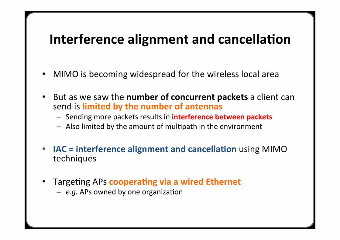
• MIMO is becoming widespread for the wireless local area
• But as we saw the number of concurrent packets a client can send is limited by the number of antennas – Sending more packets results in interference between packets – Also limited by the amount of mulHpath in the environment
• IAC = interference alignment and cancellaAon using MIMO techniques
• TargeHng APs cooperaAng via a wired Ethernet – e.g. APs owned by one organizaHon

MIMO channel representaAon
• As before, model channel from one antenna i to another j as one complex number hij
• Channel matrix H from a client to an AP is formed by [ hij ] – ConvenHon: lines in these figures don’t indicate true propagaHon
(presence/absence of mulHpath)
12h
11h
21h
22h
Client AP
10
1pH !!"
#$$%
&
21
0pH !!"
#$$%
&
p1
p2
!!"
#$$%
&=
2212
2111
hh
hhH
Figure 3: Two Packets on Uplink. The client transmits two packets,p1 and p2, from its two antennas. The packets arrive along the vectorsH[1 0]T and H[0 1]T , where H is the channel matrix and [.]T refers tothe transpose of a vector. To decode p1 and p2, the AP projects along thevectors orthogonal to H[0 1]T and H[1 0]T respectively.
802.11 channels. Similar to the current architecture, in IAC, adjacent
areas employ different 802.11 channels, but in contrast to the current
architecture, each of these areas is served by a set of APs on the same
channel, rather than a single AP. IAC allows this set of APs to serve
multiple clients at the same time despite interference. To do so, it
leverages the wired bandwidth to enable the APs to collaborate on
resolving interfering transmissions.
IAC has three components: 1) a physical layer that decodes con-
current packets across APs, 2) a MAC protocol that coordinates the
senders to transmit concurrently on the wireless medium, and 3) an
efficient mechanism to estimate channel parameters.
4 IAC’s Physical Layer
IAC modifies the physical layer to allow multiple client-AP pairs to
communicate concurrently on an 802.11 channel. IAC operates below
existing modulation and coding and is transparent to both.
For clarity, we present our ideas in the context of a 2-antenna per-
node system, and assume nodes know the channel estimates. Later,
we extend these ideas to any number of antennas and explain how we
measure channel functions. Our presentation focuses on scenarios
where interference from concurrent transmissions is much stronger
than noise and is the main factor affecting reception.
(a) Two concurrent packets on the uplink: Let us start with the
standard MIMO example in Fig. 3, where a single client transmits
two concurrent packets to an AP. Say that the client transmits p1
on the first antenna, and p2 on the second antenna. The channel
linearly combines the two packets (i.e., it linearly combines every two
digital samples of the packets). Hence, the 2-antenna AP receives the
following signals:
y1 = h11 p1 +h21 p2
y2 = h12 p1 +h22 p2,
where hi j is a complex number whose magnitude and angle refer to
the attenuation and the delay along the path from the ith antenna on
the client to the jth antenna on the AP, as shown in Fig. 3.
Since the nodes have two antennas, the transmitted and received
signals live in a 2-dimensional space. Thus, it is convenient to use 2-
dimensional vectors to represent the system [29]. This representation
will allow us to use simple figures to describe how a MIMO system
works. We can re-write the above equations as:!
y1
y2
"
= H
!
1
0
"
p1 +H
!
0
1
"
p2, (1)
where H is the 2!2 uplink channel matrix (i.e., the matrix of hi j’s).
Thus, the AP receives the sum of two vectors which are along the
directions H[1 0]T and H[0 1]T (where [.]T refers to the transpose
of a vector), as shown in Fig. 3.
1p
2p
3p
H11
H21
H12
H22
H11
1
0
! " # $ % &
H11
0
1
! " # $ % &
H21
1
0
! " # $ % &
H12
1
0
! " # $ % & H12
0
1
! " # $ % &
Clients APs
H22
H22
1
0
! " # $ % &
(a) Three Packets Without IAC.
Clients APs
111vH!
211vH!
321vH!
212vH!
322vH!
112vH!
2211vpvp!!
+
33vp!
11H
12H
22H
21H
Clients APs 322vH
(b) Three Packets With IAC.
Figure 4: Three Packets with/without IAC. In (a), the clients transmitthe packets without alignment. The packets combine at the APs alongthree different vectors and the APs cannot decode any packet. The sec-ond case shows how IAC delivers three packets on the uplink. Specifi-cally, two of the three packets are aligned at AP1, allowing AP1 to decodeone packet and send it to AP2 on the Ethernet. AP2 uses interference can-cellation to subtract the packet and decode the remaining two packets.
Assume the AP knows the channel matrix, H, (we will see how to
estimate it in §8). Decoding is easy; to decode p1, the AP needs to get
rid of the interference from p2, by projecting on a vector orthogonal to
H[0 1]T . To decode p2 it projects on a vector orthogonal to H[1 0]T .
We refer to the direction that a receiver projects on, to decode, as the
decoding vector.
(b) Three concurrent packets on the uplink: Consider what hap-
pens if another client concurrently transmits a packet, as shown in
Fig. 4a. Using the same derivation as above, AP1 receives:
!
y1
y2
"
= H11
!
1
0
"
p1 +H11
!
0
1
"
p2 +H21
!
1
0
"
p3,
where H11 and H21 are channel matrices from the first and second
clients to AP1. Said differently, AP1 receives the combination of three
packets p1, p2, and p3, along three vectors H11[1 0]T , H11[0 1]T and
H21[1 0]T , as shown in Fig. 4a. Since AP1 has only two antennas,
the received signal lives in a 2-dimensional space; hence AP1 cannot
decode three packets. Said differently, for any packet pi, the AP
cannot find a projection (decoding vector) that eliminates interference
caused by the other two packets. The second access point, AP2, is in
a similar state, it receives three packets along three vectors H12[1 0]T ,
H12[0 1]T and H22[1 0]T , and cannot decode for the same reason.
However, one advantage of MIMO is that a transmitter can control
the vectors along which its signal is received. For example, when a
transmitter transmits packet p1 on the first antenna, this is equivalent
to multiplying the samples in the packet by the unit vector [1 0]T
before transmission. As a result the received vector at the AP is
H[1 0]T p1, where H is the channel matrix from transmitter to receiver.
If the transmitter, instead, multiplies the packet p1 by a different
vector, e.g.,!v, the AP will receive the vector H!vp1. Thus, instead of
transmitting each packet on a single antenna, we multiply packet pi
by a vector!vi (i.e., multiply all digital samples in the packet by the
vector) and transmit the two elements of the resulting 2-dimensional
161
Interference alignment: IntroducAon
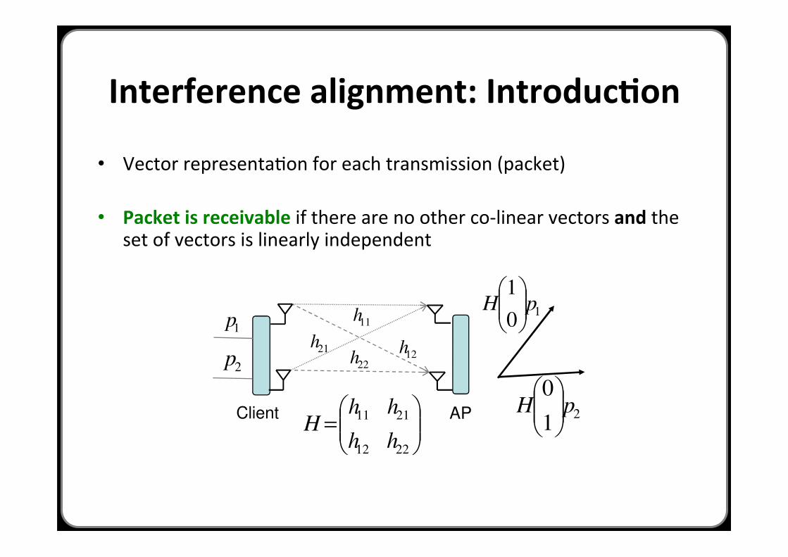
• Vector representaHon for each transmission (packet)
• Packet is receivable if there are no other co-‐linear vectors and the set of vectors is linearly independent
12h
11h
21h
22h
Client AP
10
1pH !!"
#$$%
&
21
0pH !!"
#$$%
&
p1
p2
!!"
#$$%
&=
2212
2111
hh
hhH
Figure 3: Two Packets on Uplink. The client transmits two packets,p1 and p2, from its two antennas. The packets arrive along the vectorsH[1 0]T and H[0 1]T , where H is the channel matrix and [.]T refers tothe transpose of a vector. To decode p1 and p2, the AP projects along thevectors orthogonal to H[0 1]T and H[1 0]T respectively.
802.11 channels. Similar to the current architecture, in IAC, adjacent
areas employ different 802.11 channels, but in contrast to the current
architecture, each of these areas is served by a set of APs on the same
channel, rather than a single AP. IAC allows this set of APs to serve
multiple clients at the same time despite interference. To do so, it
leverages the wired bandwidth to enable the APs to collaborate on
resolving interfering transmissions.
IAC has three components: 1) a physical layer that decodes con-
current packets across APs, 2) a MAC protocol that coordinates the
senders to transmit concurrently on the wireless medium, and 3) an
efficient mechanism to estimate channel parameters.
4 IAC’s Physical Layer
IAC modifies the physical layer to allow multiple client-AP pairs to
communicate concurrently on an 802.11 channel. IAC operates below
existing modulation and coding and is transparent to both.
For clarity, we present our ideas in the context of a 2-antenna per-
node system, and assume nodes know the channel estimates. Later,
we extend these ideas to any number of antennas and explain how we
measure channel functions. Our presentation focuses on scenarios
where interference from concurrent transmissions is much stronger
than noise and is the main factor affecting reception.
(a) Two concurrent packets on the uplink: Let us start with the
standard MIMO example in Fig. 3, where a single client transmits
two concurrent packets to an AP. Say that the client transmits p1
on the first antenna, and p2 on the second antenna. The channel
linearly combines the two packets (i.e., it linearly combines every two
digital samples of the packets). Hence, the 2-antenna AP receives the
following signals:
y1 = h11 p1 +h21 p2
y2 = h12 p1 +h22 p2,
where hi j is a complex number whose magnitude and angle refer to
the attenuation and the delay along the path from the ith antenna on
the client to the jth antenna on the AP, as shown in Fig. 3.
Since the nodes have two antennas, the transmitted and received
signals live in a 2-dimensional space. Thus, it is convenient to use 2-
dimensional vectors to represent the system [29]. This representation
will allow us to use simple figures to describe how a MIMO system
works. We can re-write the above equations as:!
y1
y2
"
= H
!
1
0
"
p1 +H
!
0
1
"
p2, (1)
where H is the 2!2 uplink channel matrix (i.e., the matrix of hi j’s).
Thus, the AP receives the sum of two vectors which are along the
directions H[1 0]T and H[0 1]T (where [.]T refers to the transpose
of a vector), as shown in Fig. 3.
1p
2p
3p
H11
H21
H12
H22
H11
1
0
! " # $ % &
H11
0
1
! " # $ % &
H21
1
0
! " # $ % &
H12
1
0
! " # $ % & H12
0
1
! " # $ % &
Clients APs
H22
H22
1
0
! " # $ % &
(a) Three Packets Without IAC.
Clients APs
111vH!
211vH!
321vH!
212vH!
322vH!
112vH!
2211vpvp!!
+
33vp!
11H
12H
22H
21H
Clients APs 322vH
(b) Three Packets With IAC.
Figure 4: Three Packets with/without IAC. In (a), the clients transmitthe packets without alignment. The packets combine at the APs alongthree different vectors and the APs cannot decode any packet. The sec-ond case shows how IAC delivers three packets on the uplink. Specifi-cally, two of the three packets are aligned at AP1, allowing AP1 to decodeone packet and send it to AP2 on the Ethernet. AP2 uses interference can-cellation to subtract the packet and decode the remaining two packets.
Assume the AP knows the channel matrix, H, (we will see how to
estimate it in §8). Decoding is easy; to decode p1, the AP needs to get
rid of the interference from p2, by projecting on a vector orthogonal to
H[0 1]T . To decode p2 it projects on a vector orthogonal to H[1 0]T .
We refer to the direction that a receiver projects on, to decode, as the
decoding vector.
(b) Three concurrent packets on the uplink: Consider what hap-
pens if another client concurrently transmits a packet, as shown in
Fig. 4a. Using the same derivation as above, AP1 receives:
!
y1
y2
"
= H11
!
1
0
"
p1 +H11
!
0
1
"
p2 +H21
!
1
0
"
p3,
where H11 and H21 are channel matrices from the first and second
clients to AP1. Said differently, AP1 receives the combination of three
packets p1, p2, and p3, along three vectors H11[1 0]T , H11[0 1]T and
H21[1 0]T , as shown in Fig. 4a. Since AP1 has only two antennas,
the received signal lives in a 2-dimensional space; hence AP1 cannot
decode three packets. Said differently, for any packet pi, the AP
cannot find a projection (decoding vector) that eliminates interference
caused by the other two packets. The second access point, AP2, is in
a similar state, it receives three packets along three vectors H12[1 0]T ,
H12[0 1]T and H22[1 0]T , and cannot decode for the same reason.
However, one advantage of MIMO is that a transmitter can control
the vectors along which its signal is received. For example, when a
transmitter transmits packet p1 on the first antenna, this is equivalent
to multiplying the samples in the packet by the unit vector [1 0]T
before transmission. As a result the received vector at the AP is
H[1 0]T p1, where H is the channel matrix from transmitter to receiver.
If the transmitter, instead, multiplies the packet p1 by a different
vector, e.g.,!v, the AP will receive the vector H!vp1. Thus, instead of
transmitting each packet on a single antenna, we multiply packet pi
by a vector!vi (i.e., multiply all digital samples in the packet by the
vector) and transmit the two elements of the resulting 2-dimensional
161
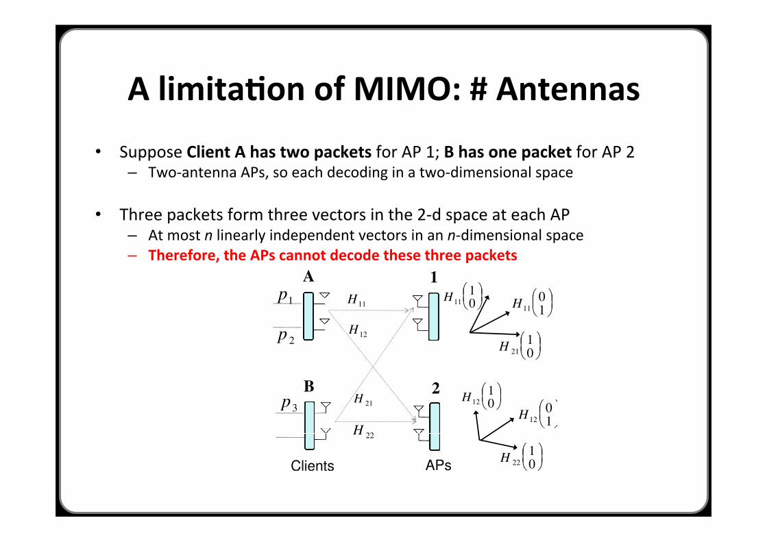
A limitaAon of MIMO: # Antennas • Suppose Client A has two packets for AP 1; B has one packet for AP 2
– Two-‐antenna APs, so each decoding in a two-‐dimensional space
• Three packets form three vectors in the 2-‐d space at each AP – At most n linearly independent vectors in an n-‐dimensional space – Therefore, the APs cannot decode these three packets
12h
11h
21h
22h
Client AP
10
1pH
21
0pH
p1
p2
=
2212
2111
hh
hhH
Figure 3: Two Packets on Uplink. The client transmits two packets,p1 and p2, from its two antennas. The packets arrive along the vectorsH[1 0]T and H[0 1]T , where H is the channel matrix and [.]T refers tothe transpose of a vector. To decode p1 and p2, the AP projects along thevectors orthogonal to H[0 1]T and H[1 0]T respectively.
802.11 channels. Similar to the current architecture, in IAC, adjacent
areas employ different 802.11 channels, but in contrast to the current
architecture, each of these areas is served by a set of APs on the same
channel, rather than a single AP. IAC allows this set of APs to serve
multiple clients at the same time despite interference. To do so, it
leverages the wired bandwidth to enable the APs to collaborate on
resolving interfering transmissions.
IAC has three components: 1) a physical layer that decodes con-
current packets across APs, 2) a MAC protocol that coordinates the
senders to transmit concurrently on the wireless medium, and 3) an
efficient mechanism to estimate channel parameters.
4 IAC’s Physical Layer
IAC modifies the physical layer to allow multiple client-AP pairs to
communicate concurrently on an 802.11 channel. IAC operates below
existing modulation and coding and is transparent to both.
For clarity, we present our ideas in the context of a 2-antenna per-
node system, and assume nodes know the channel estimates. Later,
we extend these ideas to any number of antennas and explain how we
measure channel functions. Our presentation focuses on scenarios
where interference from concurrent transmissions is much stronger
than noise and is the main factor affecting reception.
(a) Two concurrent packets on the uplink: Let us start with the
standard MIMO example in Fig. 3, where a single client transmits
two concurrent packets to an AP. Say that the client transmits p1
on the first antenna, and p2 on the second antenna. The channel
linearly combines the two packets (i.e., it linearly combines every two
digital samples of the packets). Hence, the 2-antenna AP receives the
following signals:
y1 = h11 p1 +h21 p2
y2 = h12 p1 +h22 p2,
where hi j is a complex number whose magnitude and angle refer to
the attenuation and the delay along the path from the ith antenna on
the client to the jth antenna on the AP, as shown in Fig. 3.
Since the nodes have two antennas, the transmitted and received
signals live in a 2-dimensional space. Thus, it is convenient to use 2-
dimensional vectors to represent the system [29]. This representation
will allow us to use simple figures to describe how a MIMO system
works. We can re-write the above equations as:!
y1
y2
"
= H
!
1
0
"
p1 +H
!
0
1
"
p2, (1)
where H is the 2!2 uplink channel matrix (i.e., the matrix of hi j’s).
Thus, the AP receives the sum of two vectors which are along the
directions H[1 0]T and H[0 1]T (where [.]T refers to the transpose
of a vector), as shown in Fig. 3.
1p
2p
3p
H11
H21
H12
H22
H11
1
0
H11
0
1
H21
1
0
H12
1
0
H12
0
1
Clients APs
H22
H22
1
0
(a) Three Packets Without IAC.
Clients APs
111vH
211vH
321vH
212vH
322vH
112vH
2211vpvp
+
33vp
11H
12H
22H
21H
Clients APs 322vH
(b) Three Packets With IAC.
Figure 4: Three Packets with/without IAC. In (a), the clients transmitthe packets without alignment. The packets combine at the APs alongthree different vectors and the APs cannot decode any packet. The sec-ond case shows how IAC delivers three packets on the uplink. Specifi-cally, two of the three packets are aligned at AP1, allowing AP1 to decodeone packet and send it to AP2 on the Ethernet. AP2 uses interference can-cellation to subtract the packet and decode the remaining two packets.
Assume the AP knows the channel matrix, H, (we will see how to
estimate it in §8). Decoding is easy; to decode p1, the AP needs to get
rid of the interference from p2, by projecting on a vector orthogonal to
H[0 1]T . To decode p2 it projects on a vector orthogonal to H[1 0]T .
We refer to the direction that a receiver projects on, to decode, as the
decoding vector.
(b) Three concurrent packets on the uplink: Consider what hap-
pens if another client concurrently transmits a packet, as shown in
Fig. 4a. Using the same derivation as above, AP1 receives:
!
y1
y2
"
= H11
!
1
0
"
p1 +H11
!
0
1
"
p2 +H21
!
1
0
"
p3,
where H11 and H21 are channel matrices from the first and second
clients to AP1. Said differently, AP1 receives the combination of three
packets p1, p2, and p3, along three vectors H11[1 0]T , H11[0 1]T and
H21[1 0]T , as shown in Fig. 4a. Since AP1 has only two antennas,
the received signal lives in a 2-dimensional space; hence AP1 cannot
decode three packets. Said differently, for any packet pi, the AP
cannot find a projection (decoding vector) that eliminates interference
caused by the other two packets. The second access point, AP2, is in
a similar state, it receives three packets along three vectors H12[1 0]T ,
H12[0 1]T and H22[1 0]T , and cannot decode for the same reason.
However, one advantage of MIMO is that a transmitter can control
the vectors along which its signal is received. For example, when a
transmitter transmits packet p1 on the first antenna, this is equivalent
to multiplying the samples in the packet by the unit vector [1 0]T
before transmission. As a result the received vector at the AP is
H[1 0]T p1, where H is the channel matrix from transmitter to receiver.
If the transmitter, instead, multiplies the packet p1 by a different
vector, e.g.,!v, the AP will receive the vector H!vp1. Thus, instead of
transmitting each packet on a single antenna, we multiply packet pi
by a vector!vi (i.e., multiply all digital samples in the packet by the
vector) and transmit the two elements of the resulting 2-dimensional
1
2
A
B
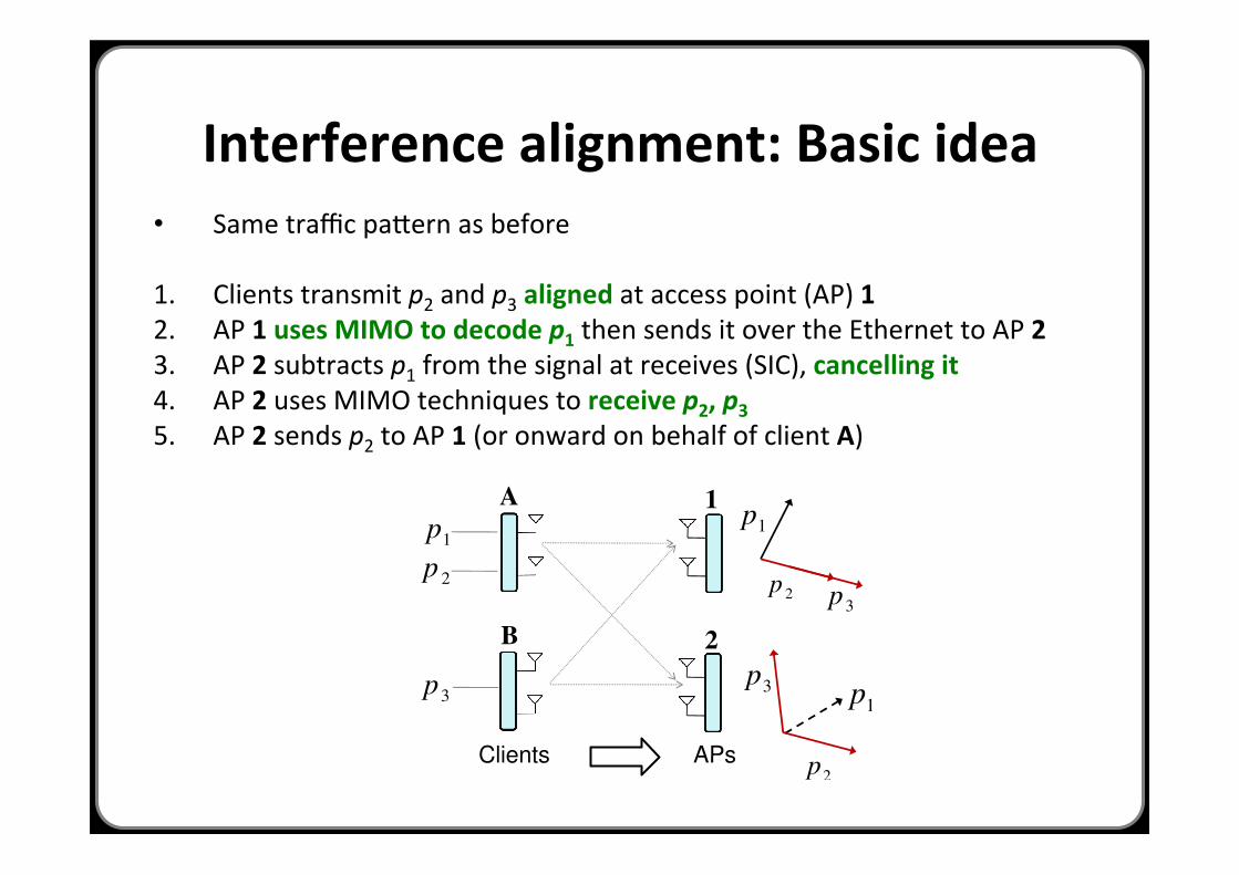
Interference alignment: Basic idea • Same traffic paSern as before
1. Clients transmit p2 and p3 aligned at access point (AP) 1 2. AP 1 uses MIMO to decode p1 then sends it over the Ethernet to AP 2 3. AP 2 subtracts p1 from the signal at receives (SIC), cancelling it 4. AP 2 uses MIMO techniques to receive p2, p3 5. AP 2 sends p2 to AP 1 (or onward on behalf of client A)
Interference Alignment and Cancellation
Shyamnath Gollakota, Samuel David Perli and Dina KatabiMIT CSAIL
ABSTRACT
The throughput of existing MIMO LANs is limited by the number of
antennas on the AP. This paper shows how to overcome this limita-
tion. It presents interference alignment and cancellation (IAC), a new
approach for decoding concurrent sender-receiver pairs in MIMO
networks. IAC synthesizes two signal processing techniques, inter-
ference alignment and interference cancellation, showing that the
combination applies to scenarios where neither interference align-
ment nor cancellation applies alone. We show analytically that IAC
almost doubles the throughput of MIMO LANs. We also implement
IAC in GNU-Radio, and experimentally demonstrate that for 2x2
MIMO LANs, IAC increases the average throughput by 1.5x on the
downlink and 2x on the uplink.
Categories and Subject Descriptors C.2.2 [Computer Sys-
tems Organization]: Computer-Communications Networks
General Terms Algorithms, Design, Performance, Theory
Keywords Interference Alignment, Interference Cancellation
1 Introduction
Multi-input multi-output (MIMO) technology is emerging as the nat-
ural choice for future wireless LANs. The current design, however,
merely replaces a single-antenna channel between a sender-receiver
pair with a MIMO channel. The throughput of such a design is always
limited by the number of antennas per access point (AP) [5, 29]. Intu-
itively, if each node has two antennas, the client can simultaneously
transmit two packets to the AP. The AP receives a linear combination
of the two transmitted packets, on each antenna, as shown in Fig. 1.
Hence, the AP obtains two linear equations for two unknown packets,
allowing it to decode. Transmitting more concurrent packets than
the number of antennas on the AP simply increases interference and
prevents decoding. Thus, today the throughput of all practical MIMO
LANs is limited by the number of antennas per AP.
This paper introduces Interference Alignment and Cancellation
(IAC), a practical scheme to overcome the antennas-per-AP through-
put limit in MIMO LANs. IAC synthesizes two interference manage-
ment techniques: interference alignment and interference cancella-
tion, showing that the combination improves performance in scenarios
where neither interference alignment nor cancellation applies alone.
To get a feel for how IAC works, consider again a 2-antenna client
that uploads two concurrent packets to a 2-antenna AP. Say we have
Permission to make digital or hard copies of all or part of this work for personalor classroom use is granted without fee provided that copies are not made ordistributed for profit or commercial advantage and that copies bear this noticeand the full citation on the first page. To copy otherwise, to republish, to poston servers or to redistribute to lists, requires prior specific permission and/or afee.SIGCOMM’09, August 17–21, 2009, Barcelona, Spain.Copyright 2009 ACM 978-1-60558-594-9/09/08
2211111phphy +=
2221122phphy +=
12h
11h
h21
22h
Client AP
p1
p2
1y
2y
Figure 1: Throughput of current MIMO LANs is limited by the numberof antennas per AP. The hi j’s are known channel coefficients, and thepi’s are concurrent packets. The client transmits two concurrent packets.The AP receives a different linear combination of the transmitted packetson each antenna, which it solves to obtain the packets.
Clients APs
1p
2p
3p
1p3
p
1p
2p
3p
Clients APs2p
Figure 2: IAC Example. AP1 decodes packet p1 and sends the decodedpacket on the Ethernet to AP2 which then performs interference cancel-lation to subtract p1. As a result AP2 can decode p2 and p3.
a second 2x2 client-AP pair on the same wireless channel and within
interference range. Can the second client-AP pair concurrently upload
a third packet? In existing MIMO LANs, the three concurrent packets
interfere. As a result, each of the two APs gets two linear equations
with three unknown packets, and hence cannot decode.
In contrast, IAC allows these three concurrent packets to be de-
coded. To do so, IAC exploits two properties of MIMO LANs: 1)
MIMO transmitters can control the alignment of their signals at a
receiver, and 2) APs are typically connected to a backend Ethernet,
which they can use for coordination. Thus, in IAC, the two clients
encode their transmissions in a special way to align the second and
the third packets at AP1 but not at AP2, as shown in Fig. 2. As a
result, AP1 can treat the second and third packets as one unknown;
i.e., AP1 has the equivalent of two equations with two unknowns,
allowing it to decode the first packet, p1. AP1 then sends the decoded
packet on the Ethernet to AP2, which can now perform interference
cancellation to subtract the effect of the known packet. As a result,
AP2 is left with two linear equations over two unknown packets, p2
and p3, which it can decode. The system delivers three packets per
time unit. Hence, its throughput is not bounded by the number of
antennas per AP.
Note the synergy between interference alignment and interference
cancellation. Interference alignment aligns a subset of the packets at
the first AP, allowing it to locally decode one packet and hence boot-
strap the decoding process. Interference cancellation enables other
APs to use the decoded packet to cancel its interference, and hence
decode more packets. Neither interference alignment nor cancellation
would be sufficient on its own to decode the three packets in Fig. 2.
1
2
A
B

The effect of interference alignment
• Transmit beamforming: client mulHplies packet by a vector v – Changes alignment at receiver
• A picks random v1 and v2; B chooses v3 so that H11v2 = H21v3
• How to find Hij? Measure the channels: channel esAmaAon
12h
11h
21h
22h
Client AP
10
1pH
21
0pH
p1
p2
=
2212
2111
hh
hhH
Figure 3: Two Packets on Uplink. The client transmits two packets,p1 and p2, from its two antennas. The packets arrive along the vectorsH[1 0]T and H[0 1]T , where H is the channel matrix and [.]T refers tothe transpose of a vector. To decode p1 and p2, the AP projects along thevectors orthogonal to H[0 1]T and H[1 0]T respectively.
802.11 channels. Similar to the current architecture, in IAC, adjacent
areas employ different 802.11 channels, but in contrast to the current
architecture, each of these areas is served by a set of APs on the same
channel, rather than a single AP. IAC allows this set of APs to serve
multiple clients at the same time despite interference. To do so, it
leverages the wired bandwidth to enable the APs to collaborate on
resolving interfering transmissions.
IAC has three components: 1) a physical layer that decodes con-
current packets across APs, 2) a MAC protocol that coordinates the
senders to transmit concurrently on the wireless medium, and 3) an
efficient mechanism to estimate channel parameters.
4 IAC’s Physical Layer
IAC modifies the physical layer to allow multiple client-AP pairs to
communicate concurrently on an 802.11 channel. IAC operates below
existing modulation and coding and is transparent to both.
For clarity, we present our ideas in the context of a 2-antenna per-
node system, and assume nodes know the channel estimates. Later,
we extend these ideas to any number of antennas and explain how we
measure channel functions. Our presentation focuses on scenarios
where interference from concurrent transmissions is much stronger
than noise and is the main factor affecting reception.
(a) Two concurrent packets on the uplink: Let us start with the
standard MIMO example in Fig. 3, where a single client transmits
two concurrent packets to an AP. Say that the client transmits p1
on the first antenna, and p2 on the second antenna. The channel
linearly combines the two packets (i.e., it linearly combines every two
digital samples of the packets). Hence, the 2-antenna AP receives the
following signals:
y1 = h11 p1 +h21 p2
y2 = h12 p1 +h22 p2,
where hi j is a complex number whose magnitude and angle refer to
the attenuation and the delay along the path from the ith antenna on
the client to the jth antenna on the AP, as shown in Fig. 3.
Since the nodes have two antennas, the transmitted and received
signals live in a 2-dimensional space. Thus, it is convenient to use 2-
dimensional vectors to represent the system [29]. This representation
will allow us to use simple figures to describe how a MIMO system
works. We can re-write the above equations as:!
y1
y2
"
= H
!
1
0
"
p1 +H
!
0
1
"
p2, (1)
where H is the 2!2 uplink channel matrix (i.e., the matrix of hi j’s).
Thus, the AP receives the sum of two vectors which are along the
directions H[1 0]T and H[0 1]T (where [.]T refers to the transpose
of a vector), as shown in Fig. 3.
1p
2p
3p
H11
H21
H12
H22
H11
1
0
H11
0
1
H21
1
0
H12
1
0
H12
0
1
Clients APs
H22
H22
1
0
(a) Three Packets Without IAC.
Clients APs
111vH
211vH
321vH
212vH
322vH
112vH
2211vpvp
+
33vp
11H
12H
22H
21H
Clients APs 322vH
(b) Three Packets With IAC.
Figure 4: Three Packets with/without IAC. In (a), the clients transmitthe packets without alignment. The packets combine at the APs alongthree different vectors and the APs cannot decode any packet. The sec-ond case shows how IAC delivers three packets on the uplink. Specifi-cally, two of the three packets are aligned at AP1, allowing AP1 to decodeone packet and send it to AP2 on the Ethernet. AP2 uses interference can-cellation to subtract the packet and decode the remaining two packets.
Assume the AP knows the channel matrix, H, (we will see how to
estimate it in §8). Decoding is easy; to decode p1, the AP needs to get
rid of the interference from p2, by projecting on a vector orthogonal to
H[0 1]T . To decode p2 it projects on a vector orthogonal to H[1 0]T .
We refer to the direction that a receiver projects on, to decode, as the
decoding vector.
(b) Three concurrent packets on the uplink: Consider what hap-
pens if another client concurrently transmits a packet, as shown in
Fig. 4a. Using the same derivation as above, AP1 receives:
!
y1
y2
"
= H11
!
1
0
"
p1 +H11
!
0
1
"
p2 +H21
!
1
0
"
p3,
where H11 and H21 are channel matrices from the first and second
clients to AP1. Said differently, AP1 receives the combination of three
packets p1, p2, and p3, along three vectors H11[1 0]T , H11[0 1]T and
H21[1 0]T , as shown in Fig. 4a. Since AP1 has only two antennas,
the received signal lives in a 2-dimensional space; hence AP1 cannot
decode three packets. Said differently, for any packet pi, the AP
cannot find a projection (decoding vector) that eliminates interference
caused by the other two packets. The second access point, AP2, is in
a similar state, it receives three packets along three vectors H12[1 0]T ,
H12[0 1]T and H22[1 0]T , and cannot decode for the same reason.
However, one advantage of MIMO is that a transmitter can control
the vectors along which its signal is received. For example, when a
transmitter transmits packet p1 on the first antenna, this is equivalent
to multiplying the samples in the packet by the unit vector [1 0]T
before transmission. As a result the received vector at the AP is
H[1 0]T p1, where H is the channel matrix from transmitter to receiver.
If the transmitter, instead, multiplies the packet p1 by a different
vector, e.g.,!v, the AP will receive the vector H!vp1. Thus, instead of
transmitting each packet on a single antenna, we multiply packet pi
by a vector!vi (i.e., multiply all digital samples in the packet by the
vector) and transmit the two elements of the resulting 2-dimensional
Without interference alignment With interference alignment A
B
1
2
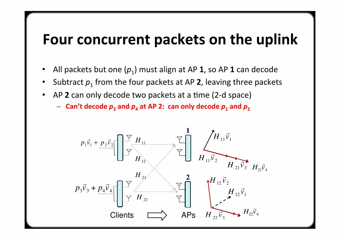
Four concurrent packets on the uplink
• All packets but one (p1) must align at AP 1, so AP 1 can decode • Subtract p1 from the four packets at AP 2, leaving three packets • AP 2 can only decode two packets at a Hme (2-‐d space)
– Can’t decode p3 and p4 at AP 2: can only decode p1 and p2
12h
11h
21h
22h
Client AP
10
1pH
21
0pH
p1
p2
=
2212
2111
hh
hhH
Figure 3: Two Packets on Uplink. The client transmits two packets,p1 and p2, from its two antennas. The packets arrive along the vectorsH[1 0]T and H[0 1]T , where H is the channel matrix and [.]T refers tothe transpose of a vector. To decode p1 and p2, the AP projects along thevectors orthogonal to H[0 1]T and H[1 0]T respectively.
802.11 channels. Similar to the current architecture, in IAC, adjacent
areas employ different 802.11 channels, but in contrast to the current
architecture, each of these areas is served by a set of APs on the same
channel, rather than a single AP. IAC allows this set of APs to serve
multiple clients at the same time despite interference. To do so, it
leverages the wired bandwidth to enable the APs to collaborate on
resolving interfering transmissions.
IAC has three components: 1) a physical layer that decodes con-
current packets across APs, 2) a MAC protocol that coordinates the
senders to transmit concurrently on the wireless medium, and 3) an
efficient mechanism to estimate channel parameters.
4 IAC’s Physical Layer
IAC modifies the physical layer to allow multiple client-AP pairs to
communicate concurrently on an 802.11 channel. IAC operates below
existing modulation and coding and is transparent to both.
For clarity, we present our ideas in the context of a 2-antenna per-
node system, and assume nodes know the channel estimates. Later,
we extend these ideas to any number of antennas and explain how we
measure channel functions. Our presentation focuses on scenarios
where interference from concurrent transmissions is much stronger
than noise and is the main factor affecting reception.
(a) Two concurrent packets on the uplink: Let us start with the
standard MIMO example in Fig. 3, where a single client transmits
two concurrent packets to an AP. Say that the client transmits p1
on the first antenna, and p2 on the second antenna. The channel
linearly combines the two packets (i.e., it linearly combines every two
digital samples of the packets). Hence, the 2-antenna AP receives the
following signals:
y1 = h11 p1 +h21 p2
y2 = h12 p1 +h22 p2,
where hi j is a complex number whose magnitude and angle refer to
the attenuation and the delay along the path from the ith antenna on
the client to the jth antenna on the AP, as shown in Fig. 3.
Since the nodes have two antennas, the transmitted and received
signals live in a 2-dimensional space. Thus, it is convenient to use 2-
dimensional vectors to represent the system [29]. This representation
will allow us to use simple figures to describe how a MIMO system
works. We can re-write the above equations as:!
y1
y2
"
= H
!
1
0
"
p1 +H
!
0
1
"
p2, (1)
where H is the 2!2 uplink channel matrix (i.e., the matrix of hi j’s).
Thus, the AP receives the sum of two vectors which are along the
directions H[1 0]T and H[0 1]T (where [.]T refers to the transpose
of a vector), as shown in Fig. 3.
1p
2p
3p
H11
H21
H12
H22
H11
1
0
H11
0
1
H21
1
0
H12
1
0
H12
0
1
Clients APs
H22
H22
1
0
(a) Three Packets Without IAC.
Clients APs
111vH
211vH
321vH
212vH
322vH
112vH
2211vpvp
+
33vp
11H
12H
22H
21H
Clients APs 322vH
(b) Three Packets With IAC.
Figure 4: Three Packets with/without IAC. In (a), the clients transmitthe packets without alignment. The packets combine at the APs alongthree different vectors and the APs cannot decode any packet. The sec-ond case shows how IAC delivers three packets on the uplink. Specifi-cally, two of the three packets are aligned at AP1, allowing AP1 to decodeone packet and send it to AP2 on the Ethernet. AP2 uses interference can-cellation to subtract the packet and decode the remaining two packets.
Assume the AP knows the channel matrix, H, (we will see how to
estimate it in §8). Decoding is easy; to decode p1, the AP needs to get
rid of the interference from p2, by projecting on a vector orthogonal to
H[0 1]T . To decode p2 it projects on a vector orthogonal to H[1 0]T .
We refer to the direction that a receiver projects on, to decode, as the
decoding vector.
(b) Three concurrent packets on the uplink: Consider what hap-
pens if another client concurrently transmits a packet, as shown in
Fig. 4a. Using the same derivation as above, AP1 receives:
!
y1
y2
"
= H11
!
1
0
"
p1 +H11
!
0
1
"
p2 +H21
!
1
0
"
p3,
where H11 and H21 are channel matrices from the first and second
clients to AP1. Said differently, AP1 receives the combination of three
packets p1, p2, and p3, along three vectors H11[1 0]T , H11[0 1]T and
H21[1 0]T , as shown in Fig. 4a. Since AP1 has only two antennas,
the received signal lives in a 2-dimensional space; hence AP1 cannot
decode three packets. Said differently, for any packet pi, the AP
cannot find a projection (decoding vector) that eliminates interference
caused by the other two packets. The second access point, AP2, is in
a similar state, it receives three packets along three vectors H12[1 0]T ,
H12[0 1]T and H22[1 0]T , and cannot decode for the same reason.
However, one advantage of MIMO is that a transmitter can control
the vectors along which its signal is received. For example, when a
transmitter transmits packet p1 on the first antenna, this is equivalent
to multiplying the samples in the packet by the unit vector [1 0]T
before transmission. As a result the received vector at the AP is
H[1 0]T p1, where H is the channel matrix from transmitter to receiver.
If the transmitter, instead, multiplies the packet p1 by a different
vector, e.g.,!v, the AP will receive the vector H!vp1. Thus, instead of
transmitting each packet on a single antenna, we multiply packet pi
by a vector!vi (i.e., multiply all digital samples in the packet by the
vector) and transmit the two elements of the resulting 2-dimensional
€
H21 v 4
€
H22 v 4
1
2
€
p3 v 3 + p4
v 4
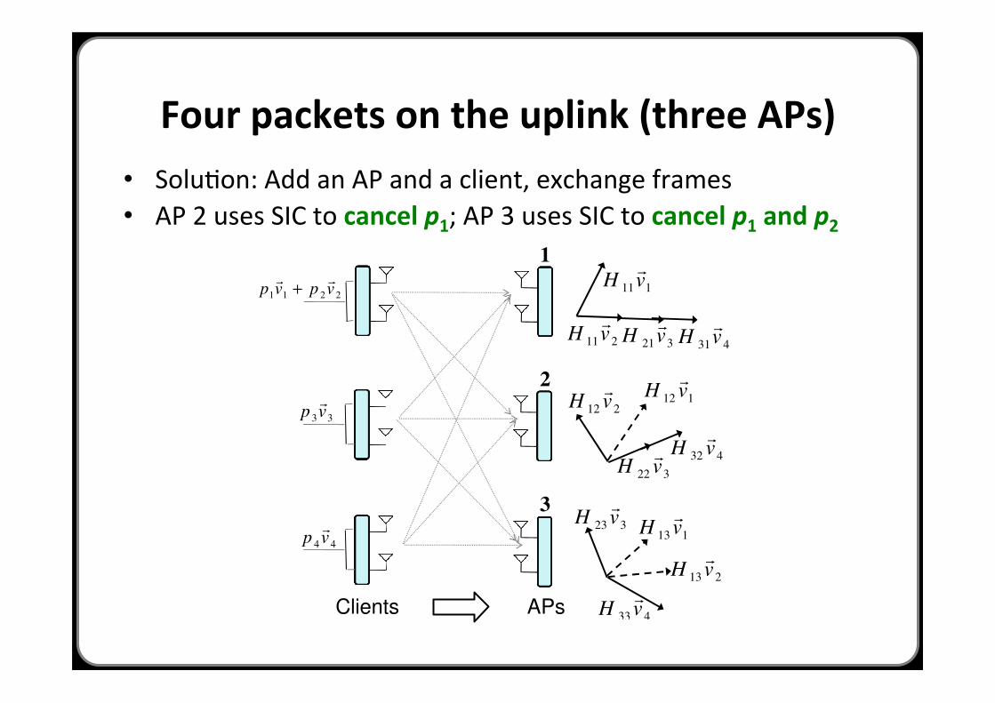
Four packets on the uplink (three APs)
111vH!
211vH!
321vH!
212vH!
432vH!
322vH!
2211vpvp!!
+
33vp! 112
vH!
431vH!
Clients APs
323vH!
44vp!
433vH!
113vH!
213vH!
Figure 5: Four Packets on the Uplink. IAC allows AP1 and AP2 todecode one packet each, and AP3 to decode the two remaining packets.This requires three packets to be aligned at AP1 and two packets at AP2,which can be done by picking appropriate encoding vectors.
vector, one on each antenna. Thus, by changing!vi, we can control the
vector along which the AP receives the packet. We call the vector!vi
the encoding vector of packet i.
Now, we can apply this method to the 2-client and 2-AP system
to transmit three concurrent packets. In particular, the transmitters
multiply packet i with vector!vi, as shown in Fig. 4b. We want to pick
!v2 and!v3 such that the second and third packets (i.e., p2 and p3) are
aligned at AP1, as in Fig. 4b, that is:2
H11!v2 = H21!v3, (2)
where H11 and H21 are the channel matrices from the first and second
clients to AP1. This can be easily done by picking random (but
unequal) values for!v1 and!v2 and substituting in the above equation
to get!v3 (i.e.,!v3 = H!121 H11!v2).3
In this case, AP1 receives the second and third packets aligned on
the same direction as in Fig 4b. Thus, AP1 can decode the first packet,
p1, by projecting on a vector orthogonal to the aligned interference,
i.e., a vector orthogonal to H11!v2 and H21!v3. Since these two vectors
are already aligned, there is a vector that is orthogonal to both of them,
and thus the AP can decode. Note that without alignment, AP1 could
not decode because H11!v2 and H21!v3 would have different directions,
and no vector will be orthogonal to both.
Note that aligning two vectors with respect to AP1 does not mean
that they are aligned with respect to AP2. This is because the chan-
nels from the clients to the two APs are different and independent.
However, we do not need to align the signals at AP2. AP1 can decode
the first packet and send it to AP2 on the Ethernet. Now AP2 knows
the first packet. It also knows the channel functions (see in §8 how
we compute channel functions). Hence it can reconstruct the signal
associated with the first packet and subtract it from what it received.
This is standard interference cancellation [19, 29]. After cancellation,
AP2 is back into a scenario similar to typical MIMO, namely two
packets on two different directions, in a 2-dimensional space. Hence,
it can decode. Thus, we obtained all three packets. AP1 decoded the
first packet, and AP2 decoded the second and third.
(c) Four concurrent packets on the uplink: Let us try to increase
the number of concurrent packets on the uplink to 4. We cannot
do this with only 2 clients and 2 APs (This is because the system
2In general, aligning the directions would mean H11!v2 = !H21!v3, where ! is a scalar.Also note that the vectors are normalized to satisfy the power constraints. But for clarity,we ignore these details in our description.
3Channel matrices are typically invertible because the antennas are chosen to be morethan half a wavelength apart. If the matrix is not invertible, then you don’t really have aMIMO system because the two antennas translate into just one equation.
is already too constrained to produce the desirable alignment.) We
need to add an additional AP-client pair. For example, consider
the three APs and three clients, in Fig. 5. The first client transmits
packets p1 and p2, the second client transmits p3 and the third client
transmits the fourth packet, p4. Now that we have developed a vector
representation, it is fairly simple to produce an IAC solution for any
configuration. Specifically, as shown in Fig. 5, AP1 needs to align 3
out of 4 packets. This results in one free packet, e.g., p1, which can
be decoded with orthogonal projection, as we did earlier. From the
perspective of AP2, p1 is already decoded at AP1, and hence can be
subtracted and removed from the signal. Thus, AP2 is left with three
unknown packets. To decode one more packet, it needs to have 2 out
of 3 packets aligned, as shown in Fig. 5. From the perspective of AP3,
two packets are already decoded at AP1 and AP2, and their signal can
be canceled using interference cancellation. Thus, AP3 is left with
only two unknown packets, which it can decode. Hence, AP3 does
not need to align any packets. We can achieve the desired alignment
(i.e., the alignment in Fig. 5) by solving the following equations:
H11!v2 = H21!v3 = H31!v4 (3)
H22!v3 = H32!v4, (4)
where Hi j is the uplink channel matrix from the ith client to the jth
AP. Eqs. 3 ensures the desired alignment at AP1 and Eq. 4 ensures the
desired alignment at AP2. Effectively, this translates to three linear
equations in three unknowns (the vectors), which can be solved. Thus,
the APs can decode four concurrent packets.4
(d) The downlink: The discussion so far has focused on the uplink,
what about the downlink? Clearly the downlink is more limited,
since the clients cannot cooperate over a wired Ethernet. A client
cannot decode one packet and send it to other clients for interference
cancellation. The lack of cooperation means that the clients have to
decode independently. So, we need to align the interference at each
client to ensure that it can decode at least one packet. For a 2-antenna
system, this means that we can at best deliver 3 concurrent packets on
the downlink. This however is still higher than what can be delivered
in today’s point-to-point MIMO LANs.
Say that we want to deliver packets p1, p2, and p3 to Client 1,
Client 2, and Client 3 respectively. Each client needs to receive the
two undesired packets aligned along the same vector and the desired
packet along a different vector, as shown in Fig. 6. To achieve this
behavior, each AP transmits one of the three packets. Now the roles
are flipped: the APs are the transmitters and the clients the receivers.
Hence, each AP multiplies the transmitted packet by a vector!vi that
is carefully chosen to ensure the desired alignment. Specifically, we
need to ensure:
Hd21!v2 = Hd
31!v3 (5)
Hd12!v1 = Hd
32!v3 (6)
Hd13!v1 = Hd
23!v2, (7)
where Hdi j is the channel from the ith AP to the jth client, i.e., the
downlink channels. The three equations above align the packets at
each client to ensure that the two undesired packets are along the
same vector. These are three linear equations over three unknown
vector and can be solved using standard methods (similar to how we
solved Eqs. §3 and §4). Hence, each client can decode its desired
packet by orthogonal projection.
4 The solution to the alignment is !v4 = eig(H!132 H22H!1
21 H31), where eig(H) is an
eigen vector of H, and!v2 = H!111 H31!v4 and!v3 = H!1
21 H31!v4.
162
• SoluHon: Add an AP and a client, exchange frames • AP 2 uses SIC to cancel p1; AP 3 uses SIC to cancel p1 and p2
1
2
3
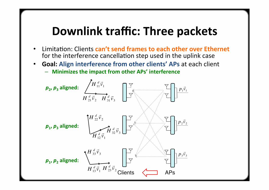
Downlink traffic: Three packets • LimitaHon: Clients can’t send frames to each other over Ethernet
for the interference cancellaHon step used in the uplink case • Goal: Align interference from other clients’ APs at each client
– Minimizes the impact from other APs’ interference
11vp!
22vp!
111vH d !
221vH d !
331vH d !
222vH d !
332vH d !
112vH d !
Clients APs
33vp!
113vH d !
333vH d !
223vH d !
Figure 6: Three Packets on the Downlink. The APs deliver one packetto each client. To enable the client to decode its packet, all the undesiredpackets at the client must be aligned.
Clients AP
2p 1
p
3p
4p
2p
1p
3p
4p
2p
1p
3p
4p
Figure 7: Four Packets on Downlink. At the first client, packets p3 andp4 are aligned along one dimension, allowing p1 and p2 to lie in a twodimensional space and hence be decoded. Similarly, at the second client,packets p1 and p2 are aligned, allowing p3 and p4 to be decoded.
5 Beyond Two Antennas
The previous section focuses on 2-antenna systems, but for the gen-
eral case of M antennas per-node, what is the maximum number of
concurrent packets that can be delivered? Further, how many APs are
needed to support such a system?
Naively, it might seem that the number of concurrent packets is
constrained only by the number of APs. Specifically, it might seem
that one can align the received packets at every AP, allowing each of
them to decode at least one packet, and hence one can keep increasing
the number of concurrent packets by increasing the number of APs.
This is however misleading because aligning a signal at one receiver
limits the ability of the transmitter to freely align it at a second
receiver. In particular, every alignment imposes new constraints on
the encoding vectors at the transmitter. For a feasible solution, the
constraints should stay fewer than the free variables in an encoding
vector. Since the encoding vector has as many variables as there are
antennas on the node, the number of constraints cannot exceed the
number of antennas. Thus, using more APs is beneficial but only up
to a point, after which one needs to increase the number of antennas.
Below, we demonstrate that in IAC, the number of concurrent packets
can be almost twice the number of antennas, and that this gain is
achieved with a relatively small number of APs.
(a) Downlink. In [15], we prove the following:
Lemma 5.1 In a system with M antennas per node, the maximum
number of concurrent packets IAC can deliver on the downlink is
max{2M!2," 32 M#}. For M > 2, IAC achieves this with M!1 APs.
For M = 3, the above lemma tells us that we can achieve 4 concurrent
packets on the downlink. Fig. 7 shows the downlink case. We have
two APs and two clients. Each AP transmits two packets, one for
each client. Since the clients have three antennas, the signal is in a
3p
1p
2p
4p
p
2p
1p
6p
4p
5p
3p
5p
3p
2p
4p
6p
1p
2p
Clients AP
5p
6p
5p
3p
2
1p
4p
6p
Figure 8: Six Packets on Uplink. At AP1, all the packets other than p1
are aligned on a two dimensional plane, allowing p1 to be decoded. AtAP2, p2, p4 and p6 are aligned along, allowing p3 and p5 to be decoded.At AP3, we cancel p1, p3 and p5 leaving p2, p4 and p6 to lie along threedifferent dimensions and be decoded.
three dimensional space. Thus, if we align two packets along one
dimension, the other two packets are free of interference and can be
decoded, resulting in 4 concurrent packets.
The above procedure can be generalized to any number of antennas.
Specifically, if we have M!1 APs and two clients, a procedure that
makes each AP transmit a packet to each client can deliver a total of
2M!2 concurrent packets across the two clients. For a large M, this
almost doubles the throughput of current MIMO LANs.
(b) Uplink. In [15], we prove the following:
Lemma 5.2 For a M-antenna system, three or more APs, and at least
two clients, IAC can deliver 2M concurrent packets on the uplink.
For M = 3, the above lemma tells us that we can achieve 6 concur-
rent packets on the uplink. Fig. 8 shows three clients transmitting to
three APs. At the first AP, five out of six packets are aligned in the
same plane. This leaves one packet free of interference and hence
can be decoded. From the perspective of the second AP, one packet
is already decoded and hence can be eliminated from the received
signal. Out of the five packets left, the second AP needs to have three
packets aligned along one dimension and two free packets, allowing
it to decode two packets. Finally, from the perspective of the last AP,
three packets are already decoded and hence their interference can be
eliminated. This leaves the last AP with three unknown packets in a
three dimensional system and hence it can decode all of them.
Again, this procedure can be applied independent of the number of
antennas. Specifically, one needs to align 2M packets such that the
first AP can decode one packet, the second AP decodes M!1 packets
and the last AP decodes M packets.
6 Practical Issues
The practicality of IAC relies on being able to implement interfer-
ence alignment and interference cancellation. IAC uses only the
subtraction step of interference cancellation. Interference cancella-
tion typically involves two steps: first it decodes one of the concurrent
packets in the presence of interference and second it subtracts the
decoded packet from the rest to remove its contribution to interfer-
ence, allowing the decoding of more packets. IAC replaces the first
step with interference alignment to orthogonalize interference and
eliminate its impact as it decodes one of the concurrent packets. It
uses interference cancellation only to subtract the decoded packet.
The subtraction step of interference cancellation is widely studied
and has been shown to work in practical implementations [4, 14, 18].
163
p2, p3 aligned:
p1, p3 aligned:
p1, p2 aligned:
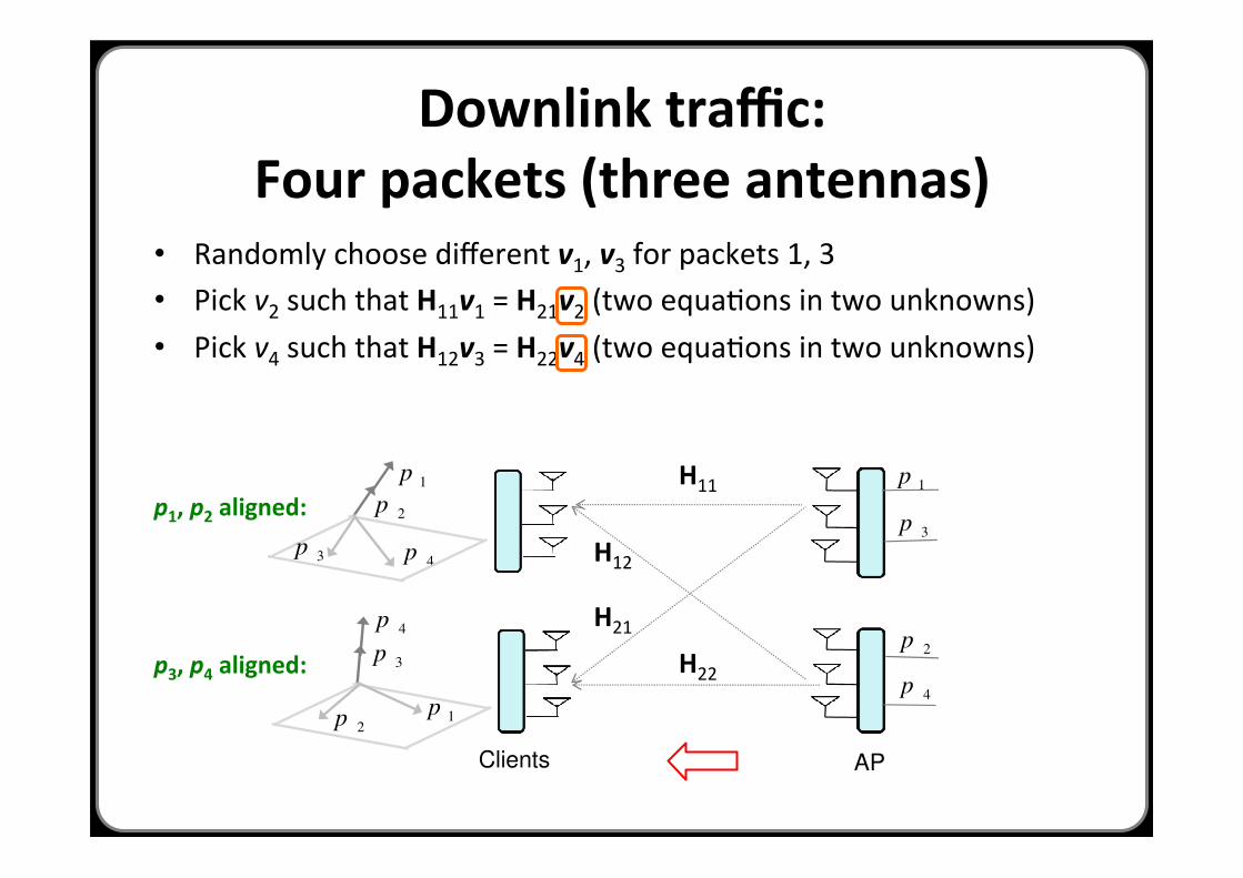
Downlink traffic: Four packets (three antennas)
• Randomly choose different v1, v3 for packets 1, 3 • Pick v2 such that H11v1 = H21v2 (two equaHons in two unknowns) • Pick v4 such that H12v3 = H22v4 (two equaHons in two unknowns)
11vp!
22vp!
111vH d !
221vH d !
331vH d !
222vH d !
332vH d !
112vH d !
Clients APs
33vp!
113vH d !
333vH d !
223vH d !
Figure 6: Three Packets on the Downlink. The APs deliver one packetto each client. To enable the client to decode its packet, all the undesiredpackets at the client must be aligned.
Clients AP
2p 1
p
3p
4p
2p
1p
3p
4p
2p
1p
3p
4p
Figure 7: Four Packets on Downlink. At the first client, packets p3 andp4 are aligned along one dimension, allowing p1 and p2 to lie in a twodimensional space and hence be decoded. Similarly, at the second client,packets p1 and p2 are aligned, allowing p3 and p4 to be decoded.
5 Beyond Two Antennas
The previous section focuses on 2-antenna systems, but for the gen-
eral case of M antennas per-node, what is the maximum number of
concurrent packets that can be delivered? Further, how many APs are
needed to support such a system?
Naively, it might seem that the number of concurrent packets is
constrained only by the number of APs. Specifically, it might seem
that one can align the received packets at every AP, allowing each of
them to decode at least one packet, and hence one can keep increasing
the number of concurrent packets by increasing the number of APs.
This is however misleading because aligning a signal at one receiver
limits the ability of the transmitter to freely align it at a second
receiver. In particular, every alignment imposes new constraints on
the encoding vectors at the transmitter. For a feasible solution, the
constraints should stay fewer than the free variables in an encoding
vector. Since the encoding vector has as many variables as there are
antennas on the node, the number of constraints cannot exceed the
number of antennas. Thus, using more APs is beneficial but only up
to a point, after which one needs to increase the number of antennas.
Below, we demonstrate that in IAC, the number of concurrent packets
can be almost twice the number of antennas, and that this gain is
achieved with a relatively small number of APs.
(a) Downlink. In [15], we prove the following:
Lemma 5.1 In a system with M antennas per node, the maximum
number of concurrent packets IAC can deliver on the downlink is
max{2M!2," 32 M#}. For M > 2, IAC achieves this with M!1 APs.
For M = 3, the above lemma tells us that we can achieve 4 concurrent
packets on the downlink. Fig. 7 shows the downlink case. We have
two APs and two clients. Each AP transmits two packets, one for
each client. Since the clients have three antennas, the signal is in a
3p
1p
2p
4p
p
2p
1p
6p
4p
5p
3p
5p
3p
2p
4p
6p
1p
2p
Clients AP
5p
6p
5p
3p
2
1p
4p
6p
Figure 8: Six Packets on Uplink. At AP1, all the packets other than p1
are aligned on a two dimensional plane, allowing p1 to be decoded. AtAP2, p2, p4 and p6 are aligned along, allowing p3 and p5 to be decoded.At AP3, we cancel p1, p3 and p5 leaving p2, p4 and p6 to lie along threedifferent dimensions and be decoded.
three dimensional space. Thus, if we align two packets along one
dimension, the other two packets are free of interference and can be
decoded, resulting in 4 concurrent packets.
The above procedure can be generalized to any number of antennas.
Specifically, if we have M!1 APs and two clients, a procedure that
makes each AP transmit a packet to each client can deliver a total of
2M!2 concurrent packets across the two clients. For a large M, this
almost doubles the throughput of current MIMO LANs.
(b) Uplink. In [15], we prove the following:
Lemma 5.2 For a M-antenna system, three or more APs, and at least
two clients, IAC can deliver 2M concurrent packets on the uplink.
For M = 3, the above lemma tells us that we can achieve 6 concur-
rent packets on the uplink. Fig. 8 shows three clients transmitting to
three APs. At the first AP, five out of six packets are aligned in the
same plane. This leaves one packet free of interference and hence
can be decoded. From the perspective of the second AP, one packet
is already decoded and hence can be eliminated from the received
signal. Out of the five packets left, the second AP needs to have three
packets aligned along one dimension and two free packets, allowing
it to decode two packets. Finally, from the perspective of the last AP,
three packets are already decoded and hence their interference can be
eliminated. This leaves the last AP with three unknown packets in a
three dimensional system and hence it can decode all of them.
Again, this procedure can be applied independent of the number of
antennas. Specifically, one needs to align 2M packets such that the
first AP can decode one packet, the second AP decodes M!1 packets
and the last AP decodes M packets.
6 Practical Issues
The practicality of IAC relies on being able to implement interfer-
ence alignment and interference cancellation. IAC uses only the
subtraction step of interference cancellation. Interference cancella-
tion typically involves two steps: first it decodes one of the concurrent
packets in the presence of interference and second it subtracts the
decoded packet from the rest to remove its contribution to interfer-
ence, allowing the decoding of more packets. IAC replaces the first
step with interference alignment to orthogonalize interference and
eliminate its impact as it decodes one of the concurrent packets. It
uses interference cancellation only to subtract the decoded packet.
The subtraction step of interference cancellation is widely studied
and has been shown to work in practical implementations [4, 14, 18].
163
H11
H22
H21
H12
p1, p2 aligned:
p3, p4 aligned:
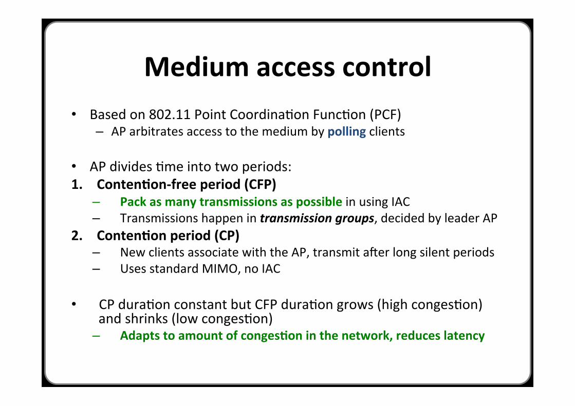
Medium access control • Based on 802.11 Point CoordinaHon FuncHon (PCF)
– AP arbitrates access to the medium by polling clients
• AP divides Hme into two periods: 1. ContenAon-‐free period (CFP)
– Pack as many transmissions as possible in using IAC – Transmissions happen in transmission groups, decided by leader AP
2. ContenAon period (CP) – New clients associate with the AP, transmit a�er long silent periods – Uses standard MIMO, no IAC
• CP duraHon constant but CFP duraHon grows (high congesHon) and shrinks (low congesHon) – Adapts to amount of congesAon in the network, reduces latency
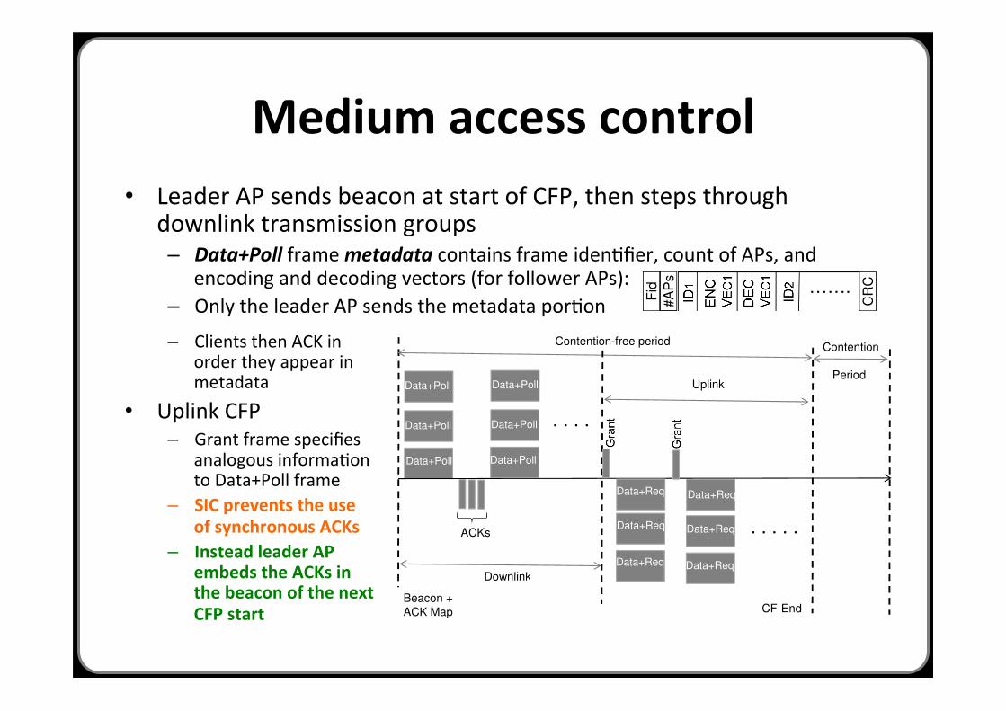
Medium access control • Leader AP sends beacon at start of CFP, then steps through
downlink transmission groups – Data+Poll frame metadata contains frame idenHfier, count of APs, and
encoding and decoding vectors (for follower APs): – Only the leader AP sends the metadata porHon
CF-End
Contention-free period Contention
Period
Downlink
Uplink
. . . .
. . . . . ACKs
Data+Req
Data+Poll
Data+Req
Data+Req
Data+Req
Data+Req
Data+Req
Data+Poll
Data+Poll
Data+Poll
Data+Poll
Data+Poll
Beacon + ACK Map CF-End
Downlink
Figure 9: IAC’s Extension to PCF.
…….
#A
Ps
CR
C
Fid
Figure 10: The metadata in a DATA+Poll frame. This metadata isbroadcast by the leader AP alone to inform the clients in a downlinktransmission group of their decoding vectors and the other APs of theirencoding vectors.
requires knowing which clients are served concurrently. This is the
job of the concurrency algorithm, which divides clients with pending
traffic into groups of concurrent transmissions that we call transmis-
sion groups. It further decides which AP serves which client in a
transmission group, and the values of the encoding and decoding vec-
tors. The process for deciding this is described in §7.2. In this section,
we focus on how to deliver packets in each transmission group.
Fig. 9 shows the series of events during a contention-free period.
At the beginning of a CFP, the leader AP sends a beacon. The leader
AP then steps through the downlink transmission groups, one at a
time, transmits their downlink packets with the help of other APs, and
polls the corresponding clients for uplink traffic. This mode is similar
to current PCF behavior, except that in the current PCF the AP steps
through a list of individual clients, one at a time; whereas in IAC the
leader AP steps through a list of transmission groups.
(b.1) Downlink. The leader AP first goes through the list of down-
link transmission groups. With the help of other APs, it sends a
DATA+Poll frame to each group. This frame has two parts. The
first part, shown in Fig. 10, is broadcast by the leader AP alone, and
contains the ids of the clients in the group and their encoding and
decoding vectors. The ids are given to the clients upon association.
The encoding and decoding vectors are computed by the concurrency
algorithm which runs on the leader AP. The leader AP also includes a
frame id, Fid, the number of APs and a checksum of its broadcast.
Further, it sets the length of the DATA+Poll frame to the maximum
length of the packets in the transmission group, so that all clients know
when the frame ends. The second part of the frame is the combination
of concurrent transmissions by all APs. For the example of three APs
with 2-antennas each, this part has the three APs transmitting a packet
to each of the three clients in a transmission group.
Note that both the clients and APs listen to the leader AP as it broad-
casts the first part of the DATA+Poll frame. In order to transmit
concurrently, the APs need to learn their encoding vectors. Similarly,
the clients need to learn the decoding vectors to be able to decode
their data. The clients and APs can use the checksum to test whether
they received the correct information. Note that the transmissions still
work fine if any of the APs or the clients failed to hear the leader AP.
Specifically, the AP/client who failed to hear the leader AP, will not
transmit. The other transmissions can go as desired.
After the DATA+Poll frame, the clients in the transmission group
send their acks, one after the other, using traditional MIMO. The order
in which they transmit these acks is the same as the order of their ids
in the DATA+Poll frame. These acks are similar to synchronous
802.11 acks. In 802.11, they are sent one after each data packet. Here
the data packets are sent concurrently and all acks follow.
(b.2) Uplink. After going through all downlink groups, the leader
AP steps through the uplink groups. Similar to the downlink case, the
leader AP first broadcasts a Grant frame specifying the ids of the
clients that will transmit on the uplink, and the encoding and decoding
vectors. The other APs listen to the encoding and decoding vectors
and wait for clients’ transmissions. The clients in an uplink group
use their encoding vectors to transmit simultaneously on the uplink.
Each client transmits a Data+Req frame. This frame contains the
client’s uplink data. If the client still has traffic to send, the frame
will also contain a new request for transmission. Each AP listens to
the Data+Req frame and projects the received signal on the proper
decoding vector. This projection is orthogonal to the interfering
signals and hence it allows each AP to receive its client of interest.
One difference between the uplink and downlink is that, while each
client on the downlink can immediately ack its packet, the APs need to
decode successively using interference cancellation and hence cannot
send synchronous acks. The solution however is simple. During
the following contention period, the APs inform the leader AP of
successful receptions using Ethernet. The leader AP combines and
sends all acks at the beginning of the next CFP, by embedding them
in the beacon information as a bit map. This should not cause any
significant delay since it allows all clients in the CFP mode to learn
about their previous packet before they get to send the next packet.
At the end of CFP, the leader AP sends a CF-End frame. This
allows the clients to go back to the contention mode, where they use
traditional point-to-point MIMO. A few points are worth noting.
(a) How do we deal with lost packets and retransmissions? If a
packet is lost on the uplink, the client discovers the loss from the
lack of an ack (at the beginning of the next CFP) and asks for a new
transmission slot next time it is polled. On the downlink, the corre-
sponding AP discovers the packet loss immediately, from the lack of
a client ack, and asks the leader AP to schedule a retransmission.
(b) Is it possible for various APs to make inconsistent decisions?
Only the leader AP makes decisions, while other APs are dumb
transmitters/receivers. Similar to clients, they receive their encoding
and decoding vectors for each transmission group over the medium
and use them without any modification. They only inform the leader
AP in case a packet is lost, or the channel’s estimate has changed.
(c) How often do APs need to communicate over the Ethernet
and what do they exchange? As described in §4, APs exchange
the decoded packets over the Ethernet to perform interference can-
cellation. Further, the subordinate APs need to tell the leader AP
whenever a packet is lost or channel coefficients to a client changes
by more than a threshold value. The APs can send this information as
annotation on packets they exchange to perform cancellation.
(d) How large is the Ethernet overhead? To minimize Ethernet
overhead, IAC connects the set of APs using a hub. This design
ensures that every decoded packet is broadcast only once to all APs
and to the switch that forwards the packet to its wired/final destination.
In this design every packet is transmitted once and there is no extra
overhead. While a hub is less efficient for a general Ethernet than a
switch, it is a natural choice to connect the IAC APs. This hubbed
network is then connected to the rest of the Ethernet via a switch.
(e) How large is the wireless overhead associated with IAC’s
MAC? IAC introduces metadata to coordinate clients and APs.
165
– Clients then ACK in order they appear in metadata
• Uplink CFP – Grant frame specifies
analogous informaHon to Data+Poll frame
– SIC prevents the use of synchronous ACKs
– Instead leader AP embeds the ACKs in the beacon of the next CFP start

Concurrency algorithm: Who sends when?
• Runs at the leader AP, over a FIFO packet send queue
• Two extremes: 1. Combine transmissions in queue for best throughput
• Combinatorial complexity and is unfair to clients with a weaker channel 2. Group packets by their arrival in the send queue
• Simple and fair to all clients; but subopAmal throughput
• IAC strategy: – Always pick head-‐of-‐line client next. – Then, randomly choose two other combinaAons of concurrent
transmiSers, picking the be^er of the two choices • This comes close to opHmal: “Power of two choices” [Mitzenmacher et al.]
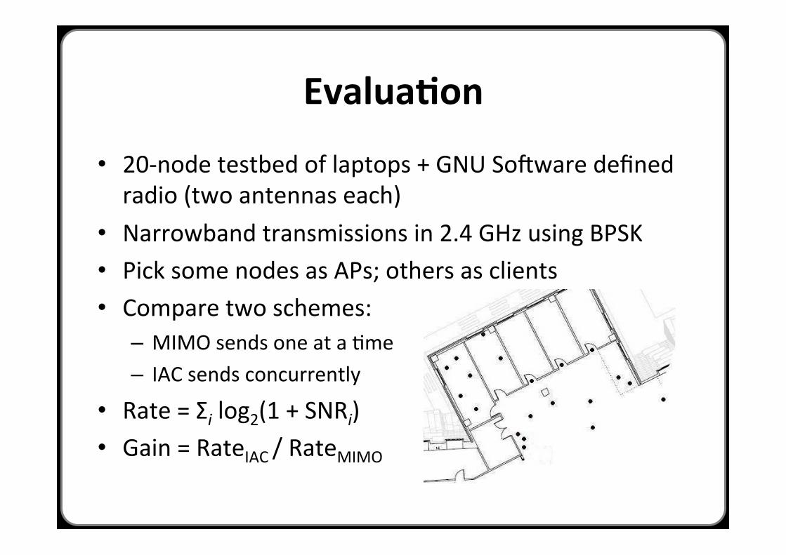
EvaluaAon
• 20-‐node testbed of laptops + GNU So�ware defined radio (two antennas each)
• Narrowband transmissions in 2.4 GHz using BPSK • Pick some nodes as APs; others as clients • Compare two schemes:
– MIMO sends one at a Hme – IAC sends concurrently
• Rate = Σi log2(1 + SNRi) • Gain = RateIAC / RateMIMO
Figure 11: Testbed Topology.
9 Complexity
IAC multiplies each packet with an encoding vector at the transmitter
and projects on a direction orthogonal to interference at the receiver.
Both pre-coding and projection are general operations in MIMO
designs [2]. IAC also performs interference cancellation, which is
linear in the number of cancelled packets. Since, the packets cancelled
at an AP are already decoded at prior APs, all the packets can be
cancelled in parallel. Hence, the delay from cancellation can be made
independent of the number of cancelled packets.
10 Performance Evaluation
We evaluate IAC in a testbed of MIMO software radios. Each node
is a laptop connected to a 2-antenna USRP radio board and runs the
GNU-Radio software. To create a MIMO node, we equip each USRP
with two RFX2400 daughterboards. We also set the MUX value in
software to allow the FPGA to process samples from both antennas.
(a) Topology. Our testbed, shown in Fig. 11, has 20 nodes. Each
node has two antennas. All nodes are within radio range of each other
to ensure that concurrent transmissions are enabled by the existence
of multiple antennas, not by spatial reuse.
(b) Modulation. IAC uses the modulation/demodulation module as
a black-box and hence works with a variety of modulation schemes.
Our implementation, however, uses BPSK, which is the modulation
scheme that 802.11 uses at low rates.
(c) Parameters. We use the default GNU-Radio parameters. How-
ever, in order to drive two antennas at the same time, we double the
interpolation and decimation rates at the transmitter and the receiver.
Each packet consists of a 32-bit preamble, and 1500-byte payload.
(d) Compared Schemes. We compare the following:• IAC: This is our implementation of IAC.
• 802.11-MIMO: There are multiple proposals for 802.11n [2, 1].
These schemes are all point-to-point, i.e., they allow only one
transmitter to access the medium at any point in time. They how-
ever differ in the amount of channel information available to the
transmitter, with more channel information leading to better perfor-
mance [29]. Since IAC uses full channel information, we compare
it with an 802.11 MIMO design with full channel information
available to both sender and receiver. This design is based on
QUALCOMM’s eigenmode enforcing [2] and uses an approach
that is proven optimal for point-to-point MIMO [29].(e) Setup. In each experiment, we randomly pick some nodes to act
as APs and others to act as clients. We repeat the same experiment
with IAC and 802.11-MIMO. Three points are worth noting.• First, we allow 802.11-MIMO access to the same number of APs
as IAC. Though 802.11-MIMO cannot use the additional APs for
concurrent transmissions, it can use them to increase diversity.
For example, if there are three APs, each 802.11-MIMO client
communicates with the AP to which it has the best SNR.
• Second, we use a simplified TDMA MAC for both IAC and 802.11-
MIMO. The MAC assigns the same number of transmission times-
lots to the two schemes. Consider an uplink scenario that involves
three clients and three APs. We start with the 802.11-MIMO exper-
iment and assign each client to its best AP. Each client transmits for
100 time slots, for a total of 300 time slots for the 802.11-MIMO
experiment. We follow with an IAC experiment where clients
transmit together for a total of 300 time slots. We then repeat the
experiment for a different client set. This simplified MAC allows
for a fair comparison between IAC and 802.11-MIMO because it
assigns the medium equally to each scheme. Implementing the
MAC in §7 requires access to accurate timing information, and
the ability to quickly switch the board from a transmit mode to a
receive mode. These requirements are not supported by the current
USRP-GNU-Radio platform.
• Finally, both IAC and 802.11-MIMO use the GNU-Radio basic
decoding modules (e.g., packet detection, clock recovery, synchro-
nization, and channel estimation) and the same system parameters.
(f) Metric. It is typical in the networking community to compare
the throughput of various designs. Throughput results, however,
do not bring much insight for radios that do not have proper rate
adaptation. Specifically, both in theory and practice, wireless systems
(e.g., 802.11a/b/g/n cards, WiMax, etc.) can exploit a higher SNR to
use denser modulation and coding schemes, and hence increase their
throughput. GNU-Radios however do not yet support rate adaptation.
In this case, it is not sufficient to compare throughput because two
systems may have the same throughput yet one of them has a higher
SNR. In an actual wireless product, the higher SNR system would use
better modulation and coding schemes to achieve a higher throughput
but current GNU Radios cannot exploit this higher SNR. Another
way to look at the problem is as follows. Say we take a 2-antenna
system and show that IAC can decode four concurrent packets, while
802.11-MIMO decodes only 2 concurrent packets. In this case, the
throughput of our system will be double the throughput of 802.11-
MIMO. Such a result however is ambiguous because it is not clear
whether the 802.11-MIMO system has a higher SNR. If it does,
then 802.11-MIMO could have used denser modulation and coding
schemes, potentially doubling its throughput, or maybe tripling it.
Because of this ambiguity, it is preferable to measure performance at
the physical layer in terms of SNR or a function of it.
Thus, for both 802.11-MIMO and IAC, we measure the signal to
noise ratio, SNRMeasured , for each transmitted packet. We compute
the achievable rate, i.e., the rate that could be achieved in the presence
of optimal rate adaptation [29]:
Rate = !i
log2(1+SNRiMeasured)[bit/s/Hz], (9)
where the sum is over all concurrent packets. For each scheme, we
average the above rate over the whole experiment, and compute the
gain as the ratio of the average rate of IAC to that of 802.11-MIMO:
Gain =RateIAC
Rate802.11!MIMO. (10)
10.1 IAC’s Multiplexing Gain
The main advantage of IAC is that it increases the number of con-
current packets, i.e., it provides a multiplexing gain. In §5, we have
demonstrated this gain analytically. Here, we check it in practice.
Experiment with 2-by-2 Uplink. We randomly pick two clients
from the testbed to upload traffic to two APs, then repeat the exper-
iment with different clients and APs. We compare IAC to 802.11-
MIMO. In 802.11-MIMO, each client uses its best AP and transmits
two packets simultaneously, and the two clients alternate in using
the medium. In IAC, the two clients simultaneously transmit three
167
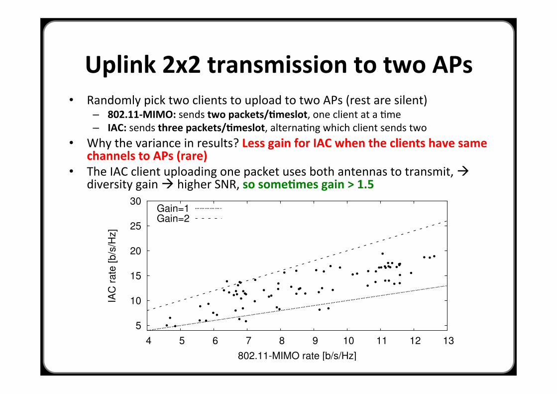
Uplink 2x2 transmission to two APs • Randomly pick two clients to upload to two APs (rest are silent)
– 802.11-‐MIMO: sends two packets/Ameslot, one client at a Hme – IAC: sends three packets/Ameslot, alternaHng which client sends two
• Why the variance in results? Less gain for IAC when the clients have same channels to APs (rare)
• The IAC client uploading one packet uses both antennas to transmit, à diversity gain à higher SNR, so someAmes gain > 1.5
5
10
15
20
25
30
4 5 6 7 8 9 10 11 12 13
IAC
ra
te [
b/s
/Hz]
802.11-MIMO rate [b/s/Hz]
Gain=1Gain=2
Figure 12: 2-Client and 2-AP Uplink. The figure shows a scatter plotof the average rate under IAC and 802.11-MIMO. The rate is measuredas bits per second per a Hz of frequency bandwidth. The two lines arefor reference; they illustrate the cases of no-gain in transfer rate, i.e.,“Gain=1” and a doubling of transfer rate, i.e., “Gain=2”. The figureshows that for the 2-client and 2-AP uplink scenario, on average, IACincreases the transfer rate by 1.5x over 802.11-MIMO.
packets to both APs, but in one time slot, client 1 uploads a single
packet and client 2 uploads two packets, while in the next slot, client
1 uploads two packets and client 2 uploads one packet.
Results for 2-by-2 Uplink. Fig. 12 shows a scatter plot of the
average rate under IAC and 802.11-MIMO. Each point on the graph
corresponds to a particular 2-client and 2-AP choice, and is gener-
ated as follows. We first transmit packets using 802.11-MIMO and
measure the received SNR for each packet. We compute the 802.11-
MIMO achievable rate according to Eq. 9. Second, we repeat the
experiment for the same 2-client and 2-AP choice but with IAC. Sim-
ilarly, we measure the SNR for each received packet and compute
the achievable rate under IAC using Eq. 9. For each point in the
figure, the x-axis shows the average rate under 802.11-MIMO while
the y-axis shows the average rate under IAC.
The figure supports the analysis, showing that for the 2-client
and 2-AP uplink, IAC’s transfer rate is on average 1.5x higher than
802.11-MIMO. The figure also shows a significant variance around
the average gain, i.e., in certain experiments the gain is less than 1.5
and in others it is more. The variance in the gain is partially due to
channel and noise variations over the duration of an experiment. More
importantly, the variance is mainly due to relative differences between
the channels of the two clients in an experiment. In particular, IAC’s
gain is typically lower when the channel matrices of the two clients
are similar. To see why this is the case, consider the extreme scenario
when the two clients have exactly the same channels to the two APs
(i.e., H11 = H21 and H12 = H22). In this case, aligning the two clients
at one AP implies aligning them at the other AP, and hence you cannot
decode. In practice, two clients are unlikely to have the same channel
to both APs. However, the more similar their channel matrices, the
more the alignment is affected by noise and imperfection of channel
estimates, and hence the less the gain from IAC. On the other hand,
IAC’s gain may exceed 1.5x because of spatial diversity. Specifically,
in IAC, one of the concurrent clients uploads two packets and the other
uploads one. The client that uploads one packet uses both antennas to
transmit. This creates a diversity gain that increases the received SNR
and the achievable rate. Thus, in addition to its multiplexing gain, IAC
can exploit diversity to achieve a higher rate for this packet, getting a
higher gain over 802.11-MIMO than analytically demonstrated. This
diversity gain is further studied in §10.2.
Experiment with 3-by-3 Uplink and Downlink. Next, we want
to check whether IAC can further increase the multiplexing gain.
In §5, we found the bound on the number of concurrent packets.
Since our nodes have 2 antennas each, we expect IAC to multiplex
4 packets on the uplink and 3 packets on the downlink. We examine
whether our implementation can deliver these rates.
5
10
15
20
25
30
4 5 6 7 8 9 10 11 12 13
IAC
ra
te [
b/s
/Hz]
802.11-MIMO rate [b/s/Hz]
Gain=1Gain=2
(a) Uplink.
5
10
15
20
25
30
4 6 8 10 12 14IA
C r
ate
[b
/s/H
z]
802.11-MIMO rate [b/s/Hz]
Gain=1Gain=2
(b) Downlink.
Figure 13: 3-clients and 3-APs. The figure shows a scatter plot of therate under IAC and 802.11-MIMO, for 3-client and 3-AP scenarios. Thetwo lines are for reference; they illustrate the cases of no-gain in trans-fer rate, i.e., “Gain=1” and a doubling of transfer rate, i.e., “Gain=2”.The results show that, on average, IAC increases the rate by 1.8x on theuplink and 1.4x on the downlink.
Each experiment involves three clients and three APs, and is run for
802.11-MIMO and then for IAC. In the 802.11-MIMO experiments,
each client accesses the medium alone and uploads/downloads 2 pack-
ets per timeslot. The medium is arbitrated between the three clients.
In IAC, all clients access the medium concurrently. In downlink
experiments, each client transmits 1 packet per timeslot. In uplink
experiments, in every timeslot, one of the clients transmits 2 packets,
the other clients transmit one packet each. We choose the client that
transmits the two packets in each timeslot in a round robin manner.
Results for 3-by-3 Uplink and Downlink. Figs. 13a and 13b
show scatter plots of the rate under IAC and 802.11-MIMO for the
3-client and 3-AP scenario. For each point, the x-axis shows the total
rate of the three clients involved in that experiment when they use
802.11-MIMO, whereas the y-axis shows the total rate of the same
clients when they use IAC. The figures show that IAC provides about
1.4x increase in transfer rate on the downlink and 1.8x on the uplink.
Furthermore, these gains are achieved at both low and high rates (i.e.,
low and high SNRs).
10.2 IAC’s Diversity Gain
Our discussion so far has focused on scenarios with multiple clients,
where IAC provides a multiplexing gain over 802.11-MIMO. But,
what if there is only one client? In this case, IAC has no multiplexing
gain over 802.11-MIMO, i.e., in both schemes, the maximum number
of concurrent packets that can be communicated to/from one client
is two (since it has 2 antennas). However, because of its ability
to coordinate multiple APs over the Ethernet, IAC still exhibits a
diversity gain over 802.11-MIMO. This diversity gain arises from
the ability to choose between transmit-receiver antenna pairs. For
example, consider the downlink when there is one client and two
APs. We want to deliver two concurrent packets to the client. 802.11-
MIMO can exploit diversity by selecting the best among the two
168
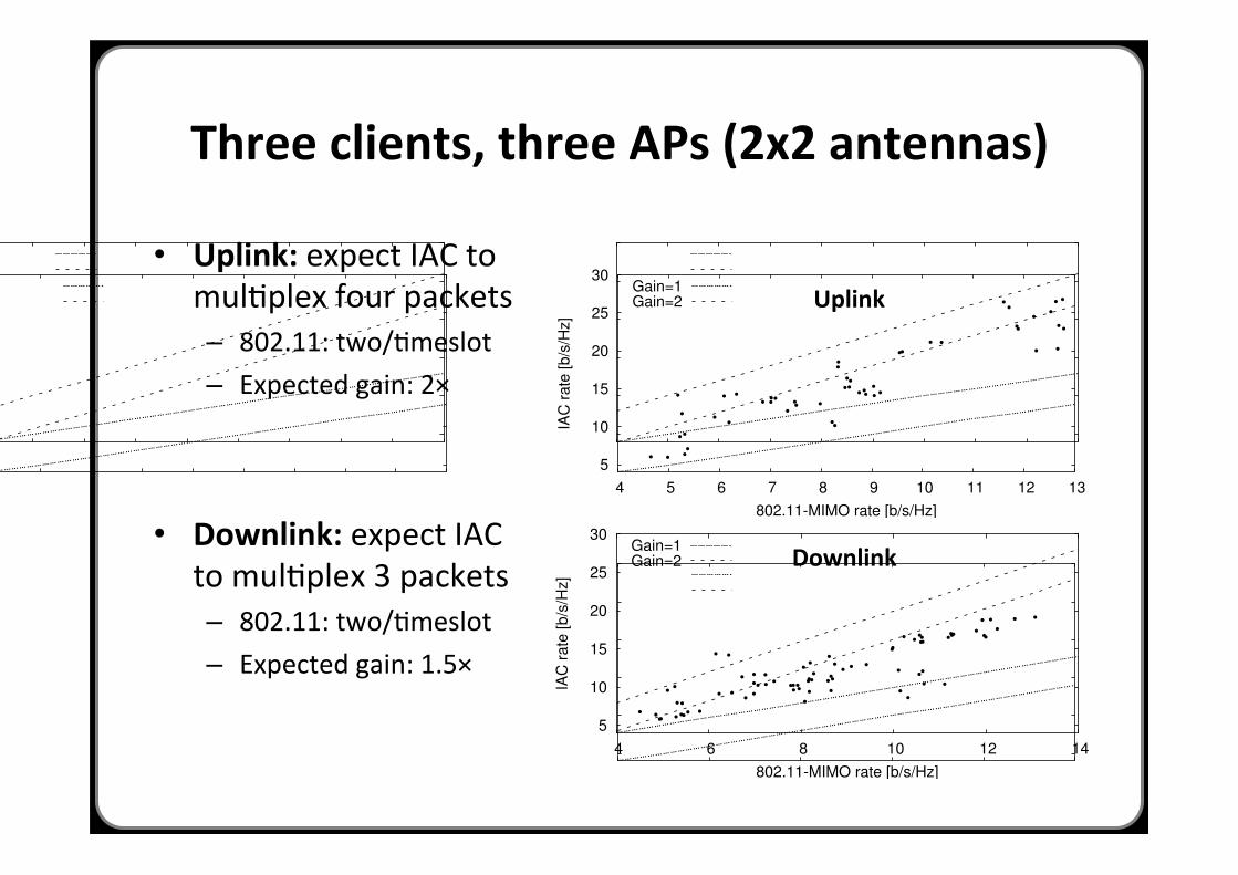
Three clients, three APs (2x2 antennas)
• Uplink: expect IAC to mulHplex four packets – 802.11: two/Hmeslot – Expected gain: 2×
• Downlink: expect IAC
to mulHplex 3 packets – 802.11: two/Hmeslot – Expected gain: 1.5×
5
10
15
20
25
30
4 5 6 7 8 9 10 11 12 13
IAC
rate
[b/s
/Hz]
802.11-MIMO rate [b/s/Hz]
Gain=1Gain=2
Figure 12: 2-Client and 2-AP Uplink. The figure shows a scatter plotof the average rate under IAC and 802.11-MIMO. The rate is measuredas bits per second per a Hz of frequency bandwidth. The two lines arefor reference; they illustrate the cases of no-gain in transfer rate, i.e.,“Gain=1” and a doubling of transfer rate, i.e., “Gain=2”. The figureshows that for the 2-client and 2-AP uplink scenario, on average, IACincreases the transfer rate by 1.5x over 802.11-MIMO.
packets to both APs, but in one time slot, client 1 uploads a single
packet and client 2 uploads two packets, while in the next slot, client
1 uploads two packets and client 2 uploads one packet.
Results for 2-by-2 Uplink. Fig. 12 shows a scatter plot of the
average rate under IAC and 802.11-MIMO. Each point on the graph
corresponds to a particular 2-client and 2-AP choice, and is gener-
ated as follows. We first transmit packets using 802.11-MIMO and
measure the received SNR for each packet. We compute the 802.11-
MIMO achievable rate according to Eq. 9. Second, we repeat the
experiment for the same 2-client and 2-AP choice but with IAC. Sim-
ilarly, we measure the SNR for each received packet and compute
the achievable rate under IAC using Eq. 9. For each point in the
figure, the x-axis shows the average rate under 802.11-MIMO while
the y-axis shows the average rate under IAC.
The figure supports the analysis, showing that for the 2-client
and 2-AP uplink, IAC’s transfer rate is on average 1.5x higher than
802.11-MIMO. The figure also shows a significant variance around
the average gain, i.e., in certain experiments the gain is less than 1.5
and in others it is more. The variance in the gain is partially due to
channel and noise variations over the duration of an experiment. More
importantly, the variance is mainly due to relative differences between
the channels of the two clients in an experiment. In particular, IAC’s
gain is typically lower when the channel matrices of the two clients
are similar. To see why this is the case, consider the extreme scenario
when the two clients have exactly the same channels to the two APs
(i.e., H11 = H21 and H12 = H22). In this case, aligning the two clients
at one AP implies aligning them at the other AP, and hence you cannot
decode. In practice, two clients are unlikely to have the same channel
to both APs. However, the more similar their channel matrices, the
more the alignment is affected by noise and imperfection of channel
estimates, and hence the less the gain from IAC. On the other hand,
IAC’s gain may exceed 1.5x because of spatial diversity. Specifically,
in IAC, one of the concurrent clients uploads two packets and the other
uploads one. The client that uploads one packet uses both antennas to
transmit. This creates a diversity gain that increases the received SNR
and the achievable rate. Thus, in addition to its multiplexing gain, IAC
can exploit diversity to achieve a higher rate for this packet, getting a
higher gain over 802.11-MIMO than analytically demonstrated. This
diversity gain is further studied in §10.2.
Experiment with 3-by-3 Uplink and Downlink. Next, we want
to check whether IAC can further increase the multiplexing gain.
In §5, we found the bound on the number of concurrent packets.
Since our nodes have 2 antennas each, we expect IAC to multiplex
4 packets on the uplink and 3 packets on the downlink. We examine
whether our implementation can deliver these rates.
5
10
15
20
25
30
4 5 6 7 8 9 10 11 12 13
IAC
rate
[b/s
/Hz]
802.11-MIMO rate [b/s/Hz]
Gain=1Gain=2
(a) Uplink.
5
10
15
20
25
30
4 6 8 10 12 14
IAC
rate
[b/s
/Hz]
802.11-MIMO rate [b/s/Hz]
Gain=1Gain=2
(b) Downlink.
Figure 13: 3-clients and 3-APs. The figure shows a scatter plot of therate under IAC and 802.11-MIMO, for 3-client and 3-AP scenarios. Thetwo lines are for reference; they illustrate the cases of no-gain in trans-fer rate, i.e., “Gain=1” and a doubling of transfer rate, i.e., “Gain=2”.The results show that, on average, IAC increases the rate by 1.8x on theuplink and 1.4x on the downlink.
Each experiment involves three clients and three APs, and is run for
802.11-MIMO and then for IAC. In the 802.11-MIMO experiments,
each client accesses the medium alone and uploads/downloads 2 pack-
ets per timeslot. The medium is arbitrated between the three clients.
In IAC, all clients access the medium concurrently. In downlink
experiments, each client transmits 1 packet per timeslot. In uplink
experiments, in every timeslot, one of the clients transmits 2 packets,
the other clients transmit one packet each. We choose the client that
transmits the two packets in each timeslot in a round robin manner.
Results for 3-by-3 Uplink and Downlink. Figs. 13a and 13b
show scatter plots of the rate under IAC and 802.11-MIMO for the
3-client and 3-AP scenario. For each point, the x-axis shows the total
rate of the three clients involved in that experiment when they use
802.11-MIMO, whereas the y-axis shows the total rate of the same
clients when they use IAC. The figures show that IAC provides about
1.4x increase in transfer rate on the downlink and 1.8x on the uplink.
Furthermore, these gains are achieved at both low and high rates (i.e.,
low and high SNRs).
10.2 IAC’s Diversity Gain
Our discussion so far has focused on scenarios with multiple clients,
where IAC provides a multiplexing gain over 802.11-MIMO. But,
what if there is only one client? In this case, IAC has no multiplexing
gain over 802.11-MIMO, i.e., in both schemes, the maximum number
of concurrent packets that can be communicated to/from one client
is two (since it has 2 antennas). However, because of its ability
to coordinate multiple APs over the Ethernet, IAC still exhibits a
diversity gain over 802.11-MIMO. This diversity gain arises from
the ability to choose between transmit-receiver antenna pairs. For
example, consider the downlink when there is one client and two
APs. We want to deliver two concurrent packets to the client. 802.11-
MIMO can exploit diversity by selecting the best among the two
168
5
10
15
20
25
30
4 5 6 7 8 9 10 11 12 13
IAC
rate
[b/s
/Hz]
802.11-MIMO rate [b/s/Hz]
Gain=1Gain=2
Figure 12: 2-Client and 2-AP Uplink. The figure shows a scatter plotof the average rate under IAC and 802.11-MIMO. The rate is measuredas bits per second per a Hz of frequency bandwidth. The two lines arefor reference; they illustrate the cases of no-gain in transfer rate, i.e.,“Gain=1” and a doubling of transfer rate, i.e., “Gain=2”. The figureshows that for the 2-client and 2-AP uplink scenario, on average, IACincreases the transfer rate by 1.5x over 802.11-MIMO.
packets to both APs, but in one time slot, client 1 uploads a single
packet and client 2 uploads two packets, while in the next slot, client
1 uploads two packets and client 2 uploads one packet.
Results for 2-by-2 Uplink. Fig. 12 shows a scatter plot of the
average rate under IAC and 802.11-MIMO. Each point on the graph
corresponds to a particular 2-client and 2-AP choice, and is gener-
ated as follows. We first transmit packets using 802.11-MIMO and
measure the received SNR for each packet. We compute the 802.11-
MIMO achievable rate according to Eq. 9. Second, we repeat the
experiment for the same 2-client and 2-AP choice but with IAC. Sim-
ilarly, we measure the SNR for each received packet and compute
the achievable rate under IAC using Eq. 9. For each point in the
figure, the x-axis shows the average rate under 802.11-MIMO while
the y-axis shows the average rate under IAC.
The figure supports the analysis, showing that for the 2-client
and 2-AP uplink, IAC’s transfer rate is on average 1.5x higher than
802.11-MIMO. The figure also shows a significant variance around
the average gain, i.e., in certain experiments the gain is less than 1.5
and in others it is more. The variance in the gain is partially due to
channel and noise variations over the duration of an experiment. More
importantly, the variance is mainly due to relative differences between
the channels of the two clients in an experiment. In particular, IAC’s
gain is typically lower when the channel matrices of the two clients
are similar. To see why this is the case, consider the extreme scenario
when the two clients have exactly the same channels to the two APs
(i.e., H11 = H21 and H12 = H22). In this case, aligning the two clients
at one AP implies aligning them at the other AP, and hence you cannot
decode. In practice, two clients are unlikely to have the same channel
to both APs. However, the more similar their channel matrices, the
more the alignment is affected by noise and imperfection of channel
estimates, and hence the less the gain from IAC. On the other hand,
IAC’s gain may exceed 1.5x because of spatial diversity. Specifically,
in IAC, one of the concurrent clients uploads two packets and the other
uploads one. The client that uploads one packet uses both antennas to
transmit. This creates a diversity gain that increases the received SNR
and the achievable rate. Thus, in addition to its multiplexing gain, IAC
can exploit diversity to achieve a higher rate for this packet, getting a
higher gain over 802.11-MIMO than analytically demonstrated. This
diversity gain is further studied in §10.2.
Experiment with 3-by-3 Uplink and Downlink. Next, we want
to check whether IAC can further increase the multiplexing gain.
In §5, we found the bound on the number of concurrent packets.
Since our nodes have 2 antennas each, we expect IAC to multiplex
4 packets on the uplink and 3 packets on the downlink. We examine
whether our implementation can deliver these rates.
5
10
15
20
25
30
4 5 6 7 8 9 10 11 12 13
IAC
rate
[b/s
/Hz]
802.11-MIMO rate [b/s/Hz]
Gain=1Gain=2
(a) Uplink.
5
10
15
20
25
30
4 6 8 10 12 14
IAC
rate
[b/s
/Hz]
802.11-MIMO rate [b/s/Hz]
Gain=1Gain=2
(b) Downlink.
Figure 13: 3-clients and 3-APs. The figure shows a scatter plot of therate under IAC and 802.11-MIMO, for 3-client and 3-AP scenarios. Thetwo lines are for reference; they illustrate the cases of no-gain in trans-fer rate, i.e., “Gain=1” and a doubling of transfer rate, i.e., “Gain=2”.The results show that, on average, IAC increases the rate by 1.8x on theuplink and 1.4x on the downlink.
Each experiment involves three clients and three APs, and is run for
802.11-MIMO and then for IAC. In the 802.11-MIMO experiments,
each client accesses the medium alone and uploads/downloads 2 pack-
ets per timeslot. The medium is arbitrated between the three clients.
In IAC, all clients access the medium concurrently. In downlink
experiments, each client transmits 1 packet per timeslot. In uplink
experiments, in every timeslot, one of the clients transmits 2 packets,
the other clients transmit one packet each. We choose the client that
transmits the two packets in each timeslot in a round robin manner.
Results for 3-by-3 Uplink and Downlink. Figs. 13a and 13b
show scatter plots of the rate under IAC and 802.11-MIMO for the
3-client and 3-AP scenario. For each point, the x-axis shows the total
rate of the three clients involved in that experiment when they use
802.11-MIMO, whereas the y-axis shows the total rate of the same
clients when they use IAC. The figures show that IAC provides about
1.4x increase in transfer rate on the downlink and 1.8x on the uplink.
Furthermore, these gains are achieved at both low and high rates (i.e.,
low and high SNRs).
10.2 IAC’s Diversity Gain
Our discussion so far has focused on scenarios with multiple clients,
where IAC provides a multiplexing gain over 802.11-MIMO. But,
what if there is only one client? In this case, IAC has no multiplexing
gain over 802.11-MIMO, i.e., in both schemes, the maximum number
of concurrent packets that can be communicated to/from one client
is two (since it has 2 antennas). However, because of its ability
to coordinate multiple APs over the Ethernet, IAC still exhibits a
diversity gain over 802.11-MIMO. This diversity gain arises from
the ability to choose between transmit-receiver antenna pairs. For
example, consider the downlink when there is one client and two
APs. We want to deliver two concurrent packets to the client. 802.11-
MIMO can exploit diversity by selecting the best among the two
168
Uplink
Downlink
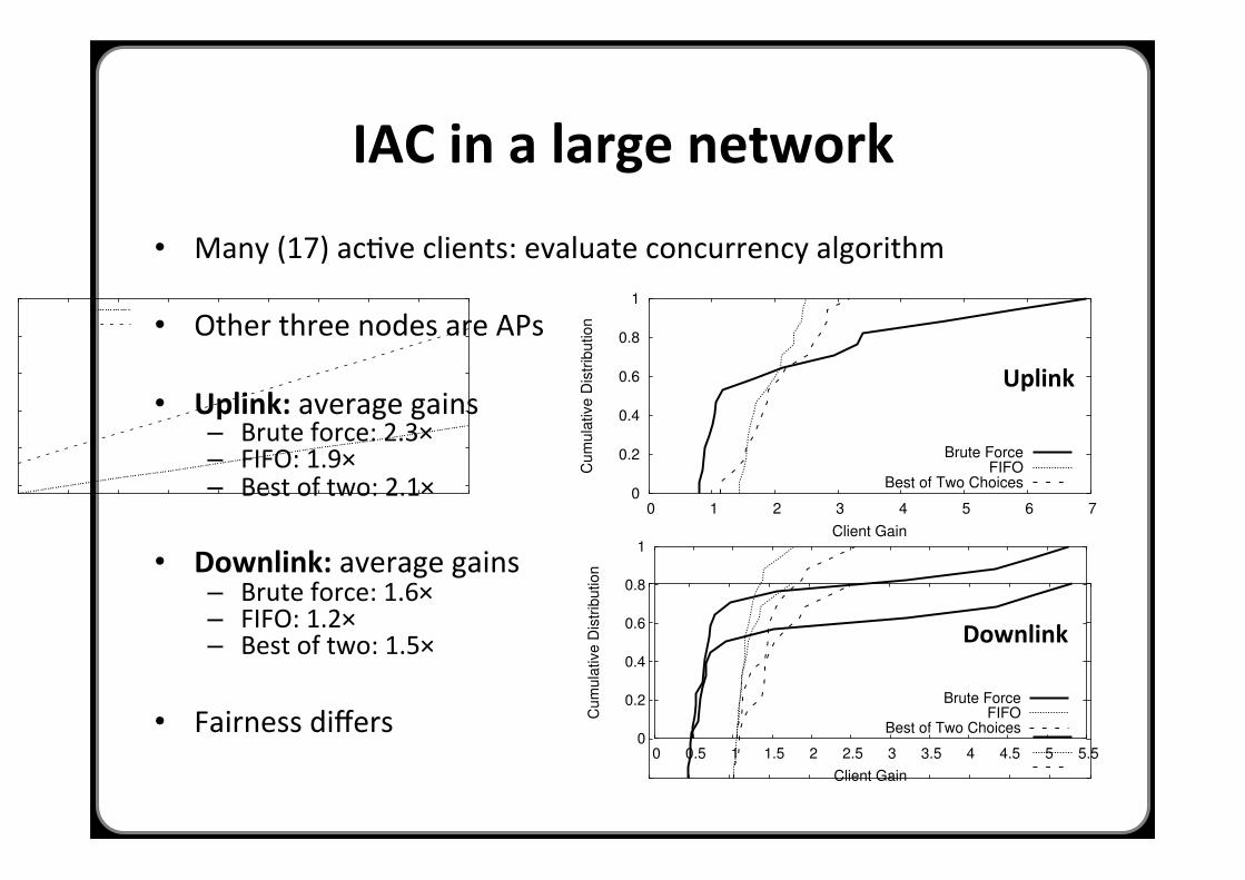
IAC in a large network
• Many (17) acHve clients: evaluate concurrency algorithm
• Other three nodes are APs
• Uplink: average gains – Brute force: 2.3× – FIFO: 1.9× – Best of two: 2.1×
• Downlink: average gains – Brute force: 1.6× – FIFO: 1.2× – Best of two: 1.5×
• Fairness differs
5
10
15
20
25
30
4 5 6 7 8 9 10 11 12 13
IAC
rate
[b/s
/Hz]
802.11-MIMO rate [b/s/Hz]
Gain=1Gain=2
Figure 14: 1-client and 2-APs. The figure shows that IAC is beneficialeven when the network has one active client. In this case, IAC providesa diversity gain over 802.11-MIMO because it allows the client to choosebetween downloading two concurrent packets from one of the two APs,or using both APs concurrently, downloading one packet from each.
APs.9 IAC however has more options because it can exploit diversity
across APs; for example it can use one antenna from each AP or use
all four antennas together or any option in between.10
Experiment with 1-client and 2-APs. Every experiment uses one
random client and two APs. The client downloads 100 packets. We
compare an 802.11-MIMO design where the client downloads its
packets from the best AP (i.e., the AP that delivers the highest SNR
to the client) with a IAC design where the two APs cooperate on
downloading the packets to the client. Specifically, the leader AP
compares the following options: transmit one packet from each AP,
and transmit both packets from one of the two APs. It picks the option
that has a better throughput. In both 802.11-MIMO and IAC, two
packets are transmitted simultaneously in every timeslot.
Results for 1-client and 2-APs. Fig. 14 plots the increase in
download rate achieved with IAC in comparison with 802.11-MIMO.
The figure reveals the following:
• IAC is beneficial even when the network has only one active client.
• IAC has a diversity gain over 802.11-MIMO. This is because
802.11-MIMO can choose only between APs, but IAC can ex-
ploit antenna diversity across APs.
• Diversity is particularly beneficial at low rates (i.e., low SNRs),
where the rate could double with IAC. This is expected since having
two diverse choices typically gives an SNR improvement of about
1-3 dB [29]. This translates to high relative gains at low SNRs, but
relatively low gains at higher SNRs.
10.3 IAC in a Large Network
We investigate IAC’s performance in a large network with many active
clients (e.g., a large conference room). When the number of clients is
larger than the maximum number of concurrent packets, one has many
options for which clients transmit concurrently, both on the uplink and
downlink. Choosing a particular option impacts both fairness and the
total rate. In fact, in any wireless network, there is always a tension
between maximizing transfer rate and ensuring fairness because the
best option in terms of rate would always transmit to the client with
the best channel and starve the others. Thus, we want to look at the
performance in terms of both fairness and rate maximization.
In particular, we compare 802.11-MIMO against three algorithms
for picking concurrent clients. All three algorithms pick the packet
at the head of the queue for transmission; however, they differ in
the choice of which other packets to concurrently transmit with the
9The literature also presents another way in which 802.11-MIMO can exploit diversity.In this case, the two antennas are used to send/receive the same packet/symbol. Thisapproach however is less desirable since it requires 802.11-MIMO to give up on sendingtwo concurrent packets, and repeat the same packet on both antennas [29].
10Note that comparing these options to find the best can be done merely by computingthe capacity using our knowledge of the channel matrices [29].
0
0.2
0.4
0.6
0.8
1
0 1 2 3 4 5 6 7
Cum
ula
tive D
istr
ibutio
n
Client Gain
Brute ForceFIFO
Best of Two Choices
(a) Uplink.
0
0.2
0.4
0.6
0.8
1
0 0.5 1 1.5 2 2.5 3 3.5 4 4.5 5 5.5
Cum
ula
tive D
istr
ibutio
n
Client Gain
Brute ForceFIFO
Best of Two Choices
(b) Downlink.
Figure 15: Gains in Transfer Rate for the Whole Testbed. The figureshows CDFs of client gains for three IAC concurrency algorithms. EachCDF is taken over 17 active clients. The figure shows that the threevariants of IAC behave differently. IAC+brute-force delivers extremegains to some clients while reducing the rate of other clients below theirrates with 802.11-MIMO. IAC+FIFO is fairer but has low overall gains.IAC+best-of-two has the best fairness-throughput tradeoff.
head-of-the-queue packet. The first algorithm is a brute force search
that finds packets in the queue that maximize the rate.11 The second
algorithm, which we refer to as FIFO, combines the packets according
to their arrival order. The third algorithm is the best of two choices,
which is explained in §7.2. This is the choice that IAC adopts.
Experiment. We use all nodes in the testbed in Fig. 11. We pick
three nodes to be APs and let the other 17 nodes be clients. Each
client has infinite demands. This ensures that a client’s throughput is
not limited by its own demands but by how the concurrency algorithm
chooses to serve the client. Packets from different clients arrive at the
system in random order. Each run involves using the medium for 1000
timeslots, and we repeat a run 3 times to compute the average rate
per client. We run the experiment with four designs: 802.11-MIMO,
IAC+best-of-two, IAC+brute-force, and IAC+FIFO. For each client,
we compute the average rate it achieves under 802.11-MIMO and
the three variants of IAC. For each variant of IAC, we compute the
change in client transfer rate in comparison to 802.11-MIMO, i.e.,
the gain seen by each client. We compare the three variants of IAC
by comparing their gains over 802.11-MIMO.
Results. Figs. 15a and 15b show the CDFs of the gains of the three
IAC concurrency algorithms with respect to 802.11-MIMO, both on
the uplink and downlink. The figures reveal the following findings:
• All three approaches for choosing concurrent packets provide a
significant gain over 802.11-MIMO. The average gain on uplink
is: 2.32x for the brute force approach, 1.9x for the FIFO approach,
and 2.08x for the best-of-two approach. Similarly, on the downlink,
the average gain is: 1.58x for the brute force approach, 1.23x for
the FIFO approach, and 1.52x for the best-of-two approach. (Note
that while IAC’s multiplexing gain is bounded by 2x, the total gain
can be larger because it includes diversity gains.)
11The relative rate can be estimated without transmitting the packets as !i log(1 +
||!vTi Hi!wi||2), where the sum is over client-AP pairs, Hi is the channel for a pair, and !vi
and !wi are the corresponding encoding and decoding vectors [29].
169
5
10
15
20
25
30
4 5 6 7 8 9 10 11 12 13
IAC
ra
te [
b/s
/Hz]
802.11-MIMO rate [b/s/Hz]
Gain=1Gain=2
Figure 14: 1-client and 2-APs. The figure shows that IAC is beneficialeven when the network has one active client. In this case, IAC providesa diversity gain over 802.11-MIMO because it allows the client to choosebetween downloading two concurrent packets from one of the two APs,or using both APs concurrently, downloading one packet from each.
APs.9 IAC however has more options because it can exploit diversity
across APs; for example it can use one antenna from each AP or use
all four antennas together or any option in between.10
Experiment with 1-client and 2-APs. Every experiment uses one
random client and two APs. The client downloads 100 packets. We
compare an 802.11-MIMO design where the client downloads its
packets from the best AP (i.e., the AP that delivers the highest SNR
to the client) with a IAC design where the two APs cooperate on
downloading the packets to the client. Specifically, the leader AP
compares the following options: transmit one packet from each AP,
and transmit both packets from one of the two APs. It picks the option
that has a better throughput. In both 802.11-MIMO and IAC, two
packets are transmitted simultaneously in every timeslot.
Results for 1-client and 2-APs. Fig. 14 plots the increase in
download rate achieved with IAC in comparison with 802.11-MIMO.
The figure reveals the following:
• IAC is beneficial even when the network has only one active client.
• IAC has a diversity gain over 802.11-MIMO. This is because
802.11-MIMO can choose only between APs, but IAC can ex-
ploit antenna diversity across APs.
• Diversity is particularly beneficial at low rates (i.e., low SNRs),
where the rate could double with IAC. This is expected since having
two diverse choices typically gives an SNR improvement of about
1-3 dB [29]. This translates to high relative gains at low SNRs, but
relatively low gains at higher SNRs.
10.3 IAC in a Large Network
We investigate IAC’s performance in a large network with many active
clients (e.g., a large conference room). When the number of clients is
larger than the maximum number of concurrent packets, one has many
options for which clients transmit concurrently, both on the uplink and
downlink. Choosing a particular option impacts both fairness and the
total rate. In fact, in any wireless network, there is always a tension
between maximizing transfer rate and ensuring fairness because the
best option in terms of rate would always transmit to the client with
the best channel and starve the others. Thus, we want to look at the
performance in terms of both fairness and rate maximization.
In particular, we compare 802.11-MIMO against three algorithms
for picking concurrent clients. All three algorithms pick the packet
at the head of the queue for transmission; however, they differ in
the choice of which other packets to concurrently transmit with the
9The literature also presents another way in which 802.11-MIMO can exploit diversity.In this case, the two antennas are used to send/receive the same packet/symbol. Thisapproach however is less desirable since it requires 802.11-MIMO to give up on sendingtwo concurrent packets, and repeat the same packet on both antennas [29].
10Note that comparing these options to find the best can be done merely by computingthe capacity using our knowledge of the channel matrices [29].
0
0.2
0.4
0.6
0.8
1
0 1 2 3 4 5 6 7
Cu
mu
lativ
e D
istr
ibu
tion
Client Gain
Brute ForceFIFO
Best of Two Choices
(a) Uplink.
0
0.2
0.4
0.6
0.8
1
0 0.5 1 1.5 2 2.5 3 3.5 4 4.5 5 5.5
Cu
mu
lativ
e D
istr
ibu
tion
Client Gain
Brute ForceFIFO
Best of Two Choices
(b) Downlink.
Figure 15: Gains in Transfer Rate for the Whole Testbed. The figureshows CDFs of client gains for three IAC concurrency algorithms. EachCDF is taken over 17 active clients. The figure shows that the threevariants of IAC behave differently. IAC+brute-force delivers extremegains to some clients while reducing the rate of other clients below theirrates with 802.11-MIMO. IAC+FIFO is fairer but has low overall gains.IAC+best-of-two has the best fairness-throughput tradeoff.
head-of-the-queue packet. The first algorithm is a brute force search
that finds packets in the queue that maximize the rate.11 The second
algorithm, which we refer to as FIFO, combines the packets according
to their arrival order. The third algorithm is the best of two choices,
which is explained in §7.2. This is the choice that IAC adopts.
Experiment. We use all nodes in the testbed in Fig. 11. We pick
three nodes to be APs and let the other 17 nodes be clients. Each
client has infinite demands. This ensures that a client’s throughput is
not limited by its own demands but by how the concurrency algorithm
chooses to serve the client. Packets from different clients arrive at the
system in random order. Each run involves using the medium for 1000
timeslots, and we repeat a run 3 times to compute the average rate
per client. We run the experiment with four designs: 802.11-MIMO,
IAC+best-of-two, IAC+brute-force, and IAC+FIFO. For each client,
we compute the average rate it achieves under 802.11-MIMO and
the three variants of IAC. For each variant of IAC, we compute the
change in client transfer rate in comparison to 802.11-MIMO, i.e.,
the gain seen by each client. We compare the three variants of IAC
by comparing their gains over 802.11-MIMO.
Results. Figs. 15a and 15b show the CDFs of the gains of the three
IAC concurrency algorithms with respect to 802.11-MIMO, both on
the uplink and downlink. The figures reveal the following findings:
• All three approaches for choosing concurrent packets provide a
significant gain over 802.11-MIMO. The average gain on uplink
is: 2.32x for the brute force approach, 1.9x for the FIFO approach,
and 2.08x for the best-of-two approach. Similarly, on the downlink,
the average gain is: 1.58x for the brute force approach, 1.23x for
the FIFO approach, and 1.52x for the best-of-two approach. (Note
that while IAC’s multiplexing gain is bounded by 2x, the total gain
can be larger because it includes diversity gains.)
11The relative rate can be estimated without transmitting the packets as !i log(1 +
||!vTi Hi!wi||2), where the sum is over client-AP pairs, Hi is the channel for a pair, and !vi
and !wi are the corresponding encoding and decoding vectors [29].
169
Uplink
Downlink

NEXT MEETING
Rateless Codes (KJ) Wednesday, 6th March 2013