Embed Size (px)
Citation preview
Orthogonality, Lommel integrals and cross product zeros of linear combinations of Bessel functionsChristian H Ziener1,2*, Felix T Kurz1,2, Lukas R Buschle1 and Thomas Kampf3
BackgroundCylindrical Bessel functions and spherical Bessel functions are widely used in mathemat-ics (Watson 1966), physics (Gray and Mathews 1895) and engineering science (McLa-chlan 1941) to analyze boundary value problems in cylindrical or spherical geometries. Using integral transform techniques or eigenfunction expansions, a second order dif-ferential equation remains that can be transformed into a cylindrical Bessel differential equation or a spherical Bessel differential equation. The general solution can be given in terms of a linear combination of cylindrical Bessel functions J and Y or, in the three-dimensional case, in terms of a linear combination of spherical Bessel functions j and y. These eigenfunctions are orthogonal to each other and the corresponding eigenvalues can be found as the zeros of a specific cross product consisting of cylindrical and spheri-cal Bessel functions, respectively. Furthermore, to calculate expansion coefficients of an eigenfunction expansion, it is helpful to evaluate Lommel integrals, which contain the eigenfunctions and a power function.
Abstract
The cylindrical Bessel differential equation and the spherical Bessel differen-tial equation in the interval R ≤ r ≤ γ R with Neumann boundary conditions are considered. The eigenfunctions are linear combinations of the Bessel function �n,ν(r) = Y ′ν(�n,ν)Jν(�n,ν r/R)− J′ν(�n,ν)Yν(�n,ν r/R) or linear combinations of the spherical Bessel functions ψm,ν(r) = y′ν(�m,ν)jν(�m,ν r/R)− j′ν(�m,ν)yν(�m,ν r/R). The orthogonality relations with analytical expressions for the normalization constant are given. Explicit expressions for the Lommel integrals in terms of Lommel functions are derived. The cross product zeros Y ′ν(�n,ν)J
′ν(γ �n,ν)− J′ν(�n,ν)Y
′ν(γ �n,ν) = 0 and
y′ν(�m,ν)j′ν(γ �m,ν)− j′ν(�m,ν)y
′ν(γ �m,ν) = 0 are considered in the complex plane for
real as well as complex values of the index ν and approximations for the exceptional zero �1,ν are obtained. A numerical scheme based on the discretization of the two-dimensional and three-dimensional Laplace operator with Neumann boundary condi-tions is presented. Explicit representations of the radial part of the Laplace operator in form of a tridiagonal matrix allow the simple computation of the cross product zeros.
Keywords: Bessel function, Linear combination, Integral
Open Access
© 2015 Ziener et al. This article is distributed under the terms of the Creative Commons Attribution 4.0 International License (http://creativecommons.org/licenses/by/4.0/), which permits unrestricted use, distribution, and reproduction in any medium, provided you give appropriate credit to the original author(s) and the source, provide a link to the Creative Commons license, and indicate if changes were made.
RESEARCH
Ziener et al. SpringerPlus (2015) 4:390 DOI 10.1186/s40064-015-1142-0
*Correspondence: [email protected] 1 Department of Radiology, German Cancer Research Center-DKFZ, Im Neuenheimer Feld 280, 69120 Heidelberg, GermanyFull list of author information is available at the end of the article
Page 2 of 26Ziener et al. SpringerPlus (2015) 4:390
Cylindrical Bessel functions and their properties are well described, as for example in the textbook of Watson (1966) where orthogonality relations and Lommel integrals are analyzed in detail. However, for a linear combination of spherical Bessel functions such orthogonality relations or Lommel integrals are not given explicitly, although they occur in many problems of diffusion or heat conduction in spherical geometries (for a review, see Carslaw and Jaeger 1959). This is mainly due to the fact that spherical Bessel func-tions with an integer index can be expressed in terms of trigonometric functions, and, thus, the remaining orthogonality relations and Lommel integrals can be given explic-itly. Yet, the case for arbitrary complex-valued indices of cylindrical and spherical Bes-sel functions has not been analyzed and there are no generally valid expressions for the orthogonality relations and the Lommel integral.
Moreover, the cross product zeros of Bessel functions that provide the eigenvalues in the case of an eigenfunction expansion are highly relevant for inverse eigenvalue prob-lems and go back to the famous question ”Can one hear the shape of a drum?” asked by Kac (1966). Cross product zeros were first analyzed by McMahon (1894) who derived an expression for large zeros. In addition, Cochran examined the asymptotic nature and analyticity of cross product Bessel functions (Cochran 1964, 1966a, b). Recurrence rela-tions for the Bessel function cross products are given by Goodwin (1949). But, until now, the cross products of cylindrical Bessel functions or spherical Bessel functions for an arbitrary complex index of the Bessel function have not yet been discussed in depth, although its application in physics becomes increasingly important, e.g. in optics or quantum mechanics, where non-hermitean potentials are involved.
In this work, the cylindrical and spherical Bessel differential equation, respectively, are considered in the radial interval R ≤ r ≤ γR where γ ≥ 1. In "Preliminary facts", we investigate the orthogonality relation between eigenfunctions and the Lommel integral for a linear combination of cylindrical Bessel functions J and Y. In an analogous pro-cedure, general expressions for the orthogonality relation and Lommel integral for a linear combination of spherical Bessel functions j and y are derived by using similarity relations between cylindrical and spherical Bessel functions. In "Cylindrical Bessel func-tions", the cylindrical Bessel differential equation R2
[ν2/r2 −�r]�n,ν(r) = �2n,ν�n,ν(r)
is considered for Neumann boundary conditions on both ends of the radial inter-val. Explicit expressions for the orthogonality relation and Lommel integral of the according eigenfunctions �n,ν(r) = Y ′
ν(�n,ν)Jν(�n,νr/R)− J ′ν(�n,ν)Yν(�n,νr/R) are given where the eigenvalues �n,ν are determined by the cross product zeros Y ′ν(�n,ν)J
′ν(γ �n,ν)− J ′ν(�n,ν)Y
′ν(γ �n,ν) = 0. To analyze cross product zeros for a com-
plex valued index ν, the function fν(�) = Y ′ν(�)J
′ν(γ �)− J ′ν(�)Y
′ν(γ �) is considered in the
complex �-plane and symmetry relations of the function fν(�) are provided. The first exceptional zero is approximated by a Taylor expansion of the function fν(�). A dis-cretization scheme for the radial part of two-dimensional Laplace-operator with Neu-mann boundary conditions is proposed and given in terms of a tridiagonal matrix. Consequently, the cross-product zeros can be obtained by solving a simple matrix eigenvalue problem. In "Spherical Bessel functions", similar results are derived for the spherical Bessel differential equation R2
[ν[ν + 1]/r2 −�r]ψm,ν(r) = �2m,νψm,ν(r) and
the corresponding eigenfunctions ψm,ν(r) = y′ν(�m,ν)jν(�m,νr/R)− j′ν(�m,ν)yν(�m,νr/R). In "Numerical implementation", numerical algorithms are provided that correctly
Page 3 of 26Ziener et al. SpringerPlus (2015) 4:390
implement discretization schemes for the radial part of the two-dimensional and three-dimensional Laplace-operator and that allow a direct determination of cross product zeros for both cylindrical and spherical Bessel functions. Applications to the diffusion process around dipole fields are described in "Application to the diffusion pro-cess around dipole fields". A summary of the results and conclusions are given in "Sum-mary and conclusions".
Preliminary factsCylindrical Bessel functions
For a linear combination of Bessel functions
the following orthogonality relation holds [see Eq. (11.4.2) on page 485 in Abramowitz and Stegun (1972) or Eq. (11) on page 135 in Watson (1966) or Eqs. (19) and (20) on page 97 in McLachlan (1941)]:
where the index ν denotes the order of the cylindrical Bessel function and n numerates the eigenvalues �n,ν which obey the boundary conditions
The normalization constant is
The Lommel integral involving the linear combination of Bessel functions and a power function is given in the following form:
which can be given in terms of the function �n,ν(z) and its derivative at the boundaries [see Eq. (5) on page 350 in paragraph 10.74 in Watson (1966) in combination with Eq. (3) on page 83 in paragraph 3.9 in Watson (1966)]. It can be evaluated using the Lommel functions
(1)�ν(z) = AJν(z)+ BYν(z)
(2)
b∫
a
dt t �n,ν(�n,νt)�n′,ν(�n′,νt) = Nn,νδnn′
(3)� ′
n,ν(�n,νa) = α�n,ν(�n,νa)
(4)� ′
n,ν(�n,νb) = β�n,ν(�n,νb) .
(5)Nn,ν =
{
t2
2
[
1−ν2
�2n,νt2
]
[�n,ν(�n,νt)]2+
t2
2
[
� ′
n,ν(�n,νt)]2}b
a
.
(6)
b∫
a
dz zκ�n,ν(z) ={
z[
�n,ν(z)S′
κ ,ν(z)−� ′
n,ν(z)Sκ ,ν(z)]}b
a
(7)
Sκ ,ν(z) = sκ ,ν(z)+ 2κ−1Ŵ
(
1+ κ − ν
2
)
Ŵ
(
1+ κ + ν
2
)
×
[
sin
(
πκ − ν
2
)
Jν(z)− cos
(
πκ − ν
2
)
Yν(z)
]
Page 4 of 26Ziener et al. SpringerPlus (2015) 4:390
The Lommel functions obey the following recurrence relations (Watson 1966; Babister 1967; Ziener and Schlemmer 2013):
For the special cases κ = 1 and ν = 2m as well as κ = 0 and ν = 2m+ 1, the Lommel functions can be written in terms of Neumann polynomials Om:
where
[see page 274 in Watson (1966)]. In a similar way the special cases κ = −1 and ν = 2m as well as κ = 0 and ν = 2m+ 1 can be written in terms of Schläfli polynomials Sm as:
where
(8)sκ ,ν(z) =zκ+1
[κ + 1]2 − ν21F2
(
1;κ − ν + 3
2,κ + ν + 3
2;−
z2
4
)
.
(9)Sκ+2,ν(z) = zκ+1−
[
[κ + 1]2 − ν2]
Sκ ,ν(z)
(10)S′κ ,ν(z)+ν
zSκ ,ν(z) = [κ + ν − 1]Sκ−1,ν−1(z)
(11)S′κ ,ν(z)−ν
zSκ ,ν(z) = [κ − ν − 1]Sκ−1,ν+1(z) .
(12)S1,2m(z) = zO2m(z)
(13)S0,2m+1(z) =z
2m+ 1O2m+1(z)
(14)O0(z) =1
z
(15)O1(z) =1
z2
(16)O2(z) =
1
z+
4
z3
...
(17)S−1,2m(z) =1
4mS2m(z)
(18)S0,2m+1(z) =1
2S2m+1(z)
(19)S0(z) = 0
(20)S1(z) =2
z
Page 5 of 26Ziener et al. SpringerPlus (2015) 4:390
[see Eq. (2) on page 285 and on page 286 in paragraph 9.3 in Watson (1966)]. The excep-tional case S−1,0(z) is treated in Watson (1966) and Glasser (2010).
The most general case in which Lommel functions Sκ ,ν can be expressed in terms of power functions occurs when the sum of the indices κ + ν = 2p+ 1 is an odd integer [see Eq. (8) in section 10.74 on page 351 in Watson (1966)]:
where the Gegenbauer polynomials An,ν are defined as [see Eq. (1) in section 9.2 on page 283 in Watson (1966)]:
From this definition it is easy to obtain the relation
and, further, to give the following explicit expressions:
The term for A0,ν(z) given in Eq. (25) is in agreement with the results of Watson [see Eq. (7) in section 9.2 on page 283 in Watson (1966)]. Other special cases of the Lommel functions can be found in section 3.10.2 on pages 111–113 in Magnus et al. (1966).
Spherical Bessel functions
To obtain similar relations for spherical Bessel functions, it is advantageous to consider the linear combination
and to use the following general relation between cylindrical Bessel functions and spher-ical Bessel functions:
(21)S2(z) =
4
z2
...
(22)Sγ ,2p+1−γ (z) =p!
21−γ Ŵ(p+ 1− γ )
zγ
2p+ 1− γA2p,1−γ (z)
(23)An,ν(z) = 2ν+n ν + n
zn+1
⌊n2 ⌋
∑
m=0
Ŵ(ν + n−m)
m!
[ z
2
]2m.
(24)A2p,1−γ (z) = zA2p+1,−γ (z) ,
(25)A0,ν(z) = Ŵ(ν + 1)2ν
z
(26)A1,ν(z) = Ŵ(ν + 2)2ν+1
z2
(27)A2,ν(z) = Ŵ(ν + 3)
4 + 4ν + z2
ν + 1
2ν
z3
...
(28)ψµ(z) = Ajµ(z)+ Byµ(z)
(29)�µ+ 1
2(z) =
√
2z
πψµ(z)
Page 6 of 26Ziener et al. SpringerPlus (2015) 4:390
Introducing the relations (29) and (30) into the orthogonality relation (2) of cylindrical Bessel functions, the following orthogonality relation for spherical Bessel functions can be obtained:
where the same notation as in the case of cylindrical Bessel functions is used, i.e. the index µ denotes the order of the spherical Bessel functions and the index m enumerates the eigenvalues �m,µ which obey the boundary condition
The corresponding normalization constant is given by
The Lommel integral can be evaluated by using Eqs. (29) and (30):
Cylindrical Bessel functionsCross‑product zeros
The cylindrical Bessel differential equation
with the radial part of two-dimensional Laplace operator �r = ∂rr + r−1∂r inside an annular ring R ≤ r ≤ γR is considered. Reflecting boundary conditions at r = R and r = γR are assumed:
(30)� ′
µ+ 12
(z) =1
√2πz
[
ψµ(z)+ 2zψ ′
µ(z)]
.
(31)
b∫
a
dt t2ψm,µ(�m,µt)ψm′,µ(�m′,µt) = Nm,µδmm′ ,
(32)ψ ′
m,µ(�m,µa) = γψm,µ(�m,µa)
(33)ψ ′
m,µ(�m,µb) = δψm,µ(�m,µb) .
(34)
Nm,µ =
{
t
2
[
t2 − µµ+ 1
�2m,µ
]
[
ψm,µ(�m,µt)]2
+t2
2�m,µψm,µ(�m,µt)ψ
′
m,µ(�m,µt)
+t3
2
[
ψ ′
m,µ(�m,µt)]2}b
a
.
(35)
b∫
a
dz zκψm,µ(z) =
{
√zψm,µ(z)
[
zS′κ− 1
2 ,µ+12
(z)−1
2Sκ− 1
2 ,µ+12(z)
]
−z√zψ ′
m,µ(z)Sκ− 12 ,µ+
12(z)
}b
a.
(36)
[
ν2
r2−�r
]
�n,ν(r) =�2n,ν
R2�n,ν(r)
(37)∂
∂r�n,ν(r)
∣
∣
∣
∣
r=R
= 0
Page 7 of 26Ziener et al. SpringerPlus (2015) 4:390
The respective eigenfunctions are given by
which obviously obey the reflecting boundary condition at r = R.Reflecting boundary conditions at the outer boundary at r = γR lead to the conditions
that have to be evaluated numerically. The function fν(�) possesses the following sym-metry properties
that translates to the properties of eigenvalues
and eigenfunctions
For real values of the Bessel function index ν the function fν(�) always takes real val-ues and the eigenvalues �n,ν are real. The respective eigenvalues �n,ν are tabulated (Bauer 1964; Bridge and Angrist 1962; Truell 1943) or they can be found by using numerical routines (Sorolla et al. 2013) and empirical approximations (Laslett and Lewish 1962). The computer algebra system MATHEMATICA® (Wolfram Research, Inc., Champaign, IL, USA, Wolfram 1999) provides the command
for numerical computation of the eigenvalues. However, these standard numerical rou-tines based on search algorithms for zeros can run into problems for inappropriate initial conditions of the algorithm. Consequently eigenvalues can be missed or found multiple. Furthermore, for complex values of the index of the Bessel functions, these numerical rou-tines often fail. To circumvent these problems, an algorithm based on solving the corre-sponding original eigenvalue problem will be introduced in "Numerical implementation".
(38)∂
∂r�n,ν(r)
∣
∣
∣
∣
r=γR
= 0 .
(39)�n,ν(r) = Y ′
ν(�n,ν)Jν
(
�n,νr
R
)
− J ′ν(�n,ν)Yν
(
�n,νr
R
)
,
(40)fν(�n,ν) = 0
(41)fν(�) = Y ′
ν(�)J′
ν(γ �)− J ′ν(�)Y′
ν(γ �) ,
(42)fν(+�) = fν(−�)
(43)f+ν(�) = f−ν(�)
(44)fν∗(�) = f ∗ν (�∗)
(45)�n,+ν = �n,−ν
(46)�n,ν∗ = �∗
n,ν
(47)�n,+ν(r) = �n,−ν(r)
(48)�n,ν∗(r) = �∗
n,ν(r) .
(49)�n,ν = BesselJPrimeYPrimeJPrimeYPrimeZeros[ν, γ ,n][[n]]
Page 8 of 26Ziener et al. SpringerPlus (2015) 4:390
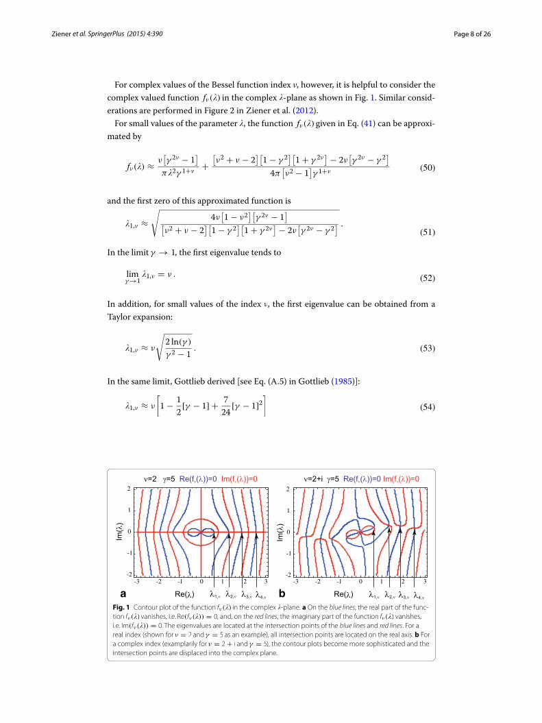
For complex values of the Bessel function index ν, however, it is helpful to consider the complex valued function fν(�) in the complex �-plane as shown in Fig. 1. Similar consid-erations are performed in Figure 2 in Ziener et al. (2012).
For small values of the parameter �, the function fν(�) given in Eq. (41) can be approxi-mated by
and the first zero of this approximated function is
In the limit γ → 1, the first eigenvalue tends to
In addition, for small values of the index ν, the first eigenvalue can be obtained from a Taylor expansion:
In the same limit, Gottlieb derived [see Eq. (A.5) in Gottlieb (1985)]:
(50)fν(�) ≈ν[
γ 2ν− 1
]
π�2γ 1+ν+
[
ν2 + ν − 2][
1− γ 2][
1+ γ 2ν]
− 2ν[
γ 2ν− γ 2
]
4π[
ν2 − 1]
γ 1+ν
(51)�1,ν ≈
√
4ν[
1− ν2][
γ 2ν − 1]
[
ν2 + ν − 2][
1− γ 2][
1+ γ 2ν]
− 2ν[
γ 2ν − γ 2] .
(52)limγ→1
�1,ν = ν .
(53)�1,ν ≈ ν
√
2 ln(γ )
γ 2 − 1.
(54)�1,ν ≈ ν
[
1−1
2[γ − 1] +
7
24[γ − 1]2
]
-3 -2 -1 0 1 2 3-2
-1
0
1
2
Im(λ
)
Re(λ)
ν=2 γ=5 Re(f (λ))=0 Im(f (λ))=0
-3 -2 -1 0 1 2 3-2
-1
0
1
2
Im(λ
)
Re(λ)
ν=2+i γ=5 Re(f (λ))=0 Im(f (λ))=0
λ1,ν λ2,ν λ3,ν λ4,ν
ν ν ν ν
a b λ1,ν λ2,ν λ3,ν λ4,ν
Fig. 1 Contour plot of the function fν(�) in the complex �-plane. a On the blue lines, the real part of the func-tion fν(�) vanishes, i.e. Re(fν(�)) = 0, and, on the red lines, the imaginary part of the function fν(�) vanishes, i.e. Im(fν(�)) = 0. The eigenvalues are located at the intersection points of the blue lines and red lines. For a real index (shown for ν = 2 and γ = 5 as an example), all intersection points are located on the real axis. b For a complex index (examplarily for ν = 2+ i and γ = 5), the contour plots become more sophisticated and the intersection points are displaced into the complex plane.
Page 9 of 26Ziener et al. SpringerPlus (2015) 4:390
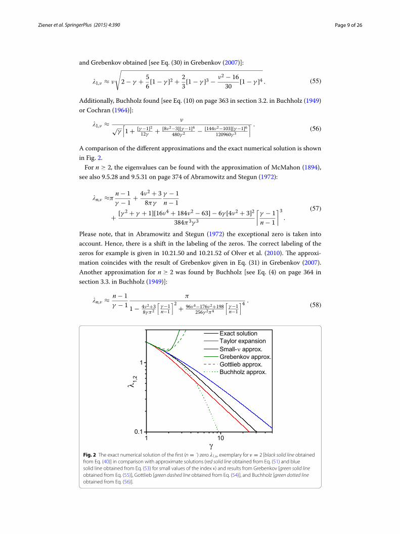
and Grebenkov obtained [see Eq. (30) in Grebenkov (2007)]:
Additionally, Buchholz found [see Eq. (10) on page 363 in section 3.2. in Buchholz (1949) or Cochran (1964)]:
A comparison of the different approximations and the exact numerical solution is shown in Fig. 2.
For n ≥ 2, the eigenvalues can be found with the approximation of McMahon (1894), see also 9.5.28 and 9.5.31 on page 374 of Abramowitz and Stegun (1972):
Please note, that in Abramowitz and Stegun (1972) the exceptional zero is taken into account. Hence, there is a shift in the labeling of the zeros. The correct labeling of the zeros for example is given in 10.21.50 and 10.21.52 of Olver et al. (2010). The approxi-mation coincides with the result of Grebenkov given in Eq. (31) in Grebenkov (2007). Another approximation for n ≥ 2 was found by Buchholz [see Eq. (4) on page 364 in section 3.3. in Buchholz (1949)]:
(55)�1,ν ≈ ν
√
2− γ +5
6[1− γ ]2 +
2
3[1− γ ]3 −
ν2 − 16
30[1− γ ]4 .
(56)�1,ν ≈
ν
√γ
[
1+ [γ−1]2
12γ +[8ν2−3][γ−1]4
480γ 2 −[144ν2−103][γ−1]6
120960γ 3
] .
(57)
�n,ν ≈πn− 1
γ − 1+
4ν2 + 3
8πγ
γ − 1
n− 1
+[γ 2
+ γ + 1][16ν4 + 184ν2 − 63] − 6γ [4ν2 + 3]2
384π3γ 3
[
γ − 1
n− 1
]3
.
(58)�n,ν ≈
n− 1
γ − 1
π
1− 4ν2+38γπ2
[
γ−1n−1
]2+
96ν4−176ν2+198256γ 2π4
[
γ−1n−1
]4.
Fig. 2 The exact numerical solution of the first (n = 1) zero �1,ν, exemplary for ν = 2 [black solid line obtained from Eq. (40)] in comparison with approximate solutions (red solid line obtained from Eq. (51) and blue solid line obtained from Eq. (53) for small values of the index ν) and results from Grebenkov [green solid line obtained from Eq. (55)], Gottlieb [green dashed line obtained from Eq. (54)], and Buchholz [green dotted line obtained from Eq. (56)].
Page 10 of 26Ziener et al. SpringerPlus (2015) 4:390
Discretization
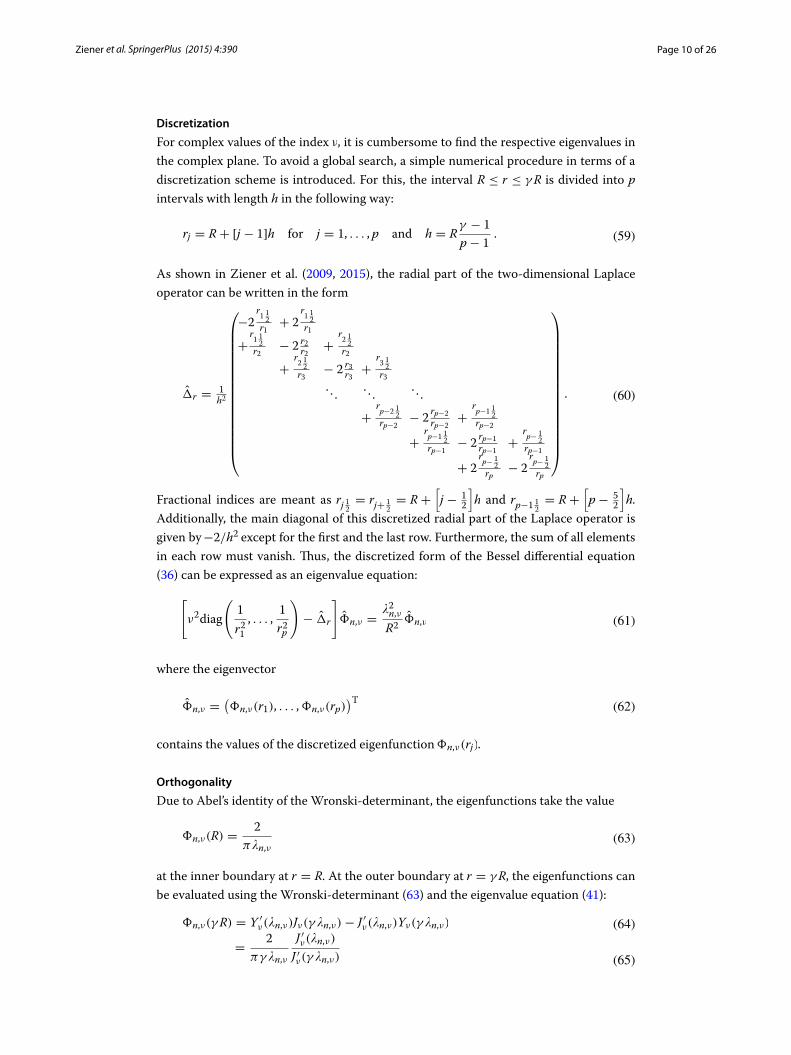
For complex values of the index ν, it is cumbersome to find the respective eigenvalues in the complex plane. To avoid a global search, a simple numerical procedure in terms of a discretization scheme is introduced. For this, the interval R ≤ r ≤ γR is divided into p intervals with length h in the following way:
As shown in Ziener et al. (2009, 2015), the radial part of the two-dimensional Laplace operator can be written in the form
Fractional indices are meant as rj 12 = rj+ 12= R+
[
j − 12
]
h and rp−1 12= R+
[
p−52
]
h. Additionally, the main diagonal of this discretized radial part of the Laplace operator is given by −2/h2 except for the first and the last row. Furthermore, the sum of all elements in each row must vanish. Thus, the discretized form of the Bessel differential equation (36) can be expressed as an eigenvalue equation:
where the eigenvector
contains the values of the discretized eigenfunction �n,ν(rj).
Orthogonality
Due to Abel’s identity of the Wronski-determinant, the eigenfunctions take the value
at the inner boundary at r = R. At the outer boundary at r = γR, the eigenfunctions can be evaluated using the Wronski-determinant (63) and the eigenvalue equation (41):
(59)rj = R+ [j − 1]h for j = 1, . . . , p and h = Rγ − 1
p− 1.
(60)�̂r =1h2
−2r1 12
r1+ 2
r1 12
r1
+
r1 12
r2− 2 r2
r2+
r2 12
r2
+
r2 12
r3− 2 r3
r3+
r3 12
r3. . .
. . .. . .
+
rp−2 1
2rp−2
− 2rp−2
rp−2+
rp−1 1
2rp−2
+
rp−1 1
2rp−1
− 2rp−1
rp−1+
rp− 1
2rp−1
+ 2rp− 1
2rp
− 2rp− 1
2rp
.
(61)
[
ν2diag
(
1
r21, . . . ,
1
r2p
)
− �̂r
]
�̂n,ν =�2n,ν
R2�̂n,ν
(62)�̂n,ν =(
�n,ν(r1), . . . ,�n,ν(rp))T
(63)�n,ν(R) =2
π�n,ν
(64)�n,ν(γR) = Y ′
ν(�n,ν)Jν(γ �n,ν)− J ′ν(�n,ν)Yν(γ �n,ν)
(65)=
2
πγ �n,ν
J ′ν(�n,ν)
J ′ν(γ �n,ν)
Page 11 of 26Ziener et al. SpringerPlus (2015) 4:390
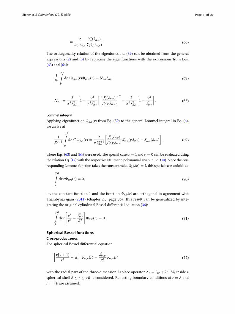
The orthogonality relation of the eigenfunctions (39) can be obtained from the general expressions (2) and (5) by replacing the eigenfunctions with the expressions from Eqs. (63) and (64):
Lommel integral
Applying eigenfunction �n,ν(r) from Eq. (39) to the general Lommel integral in Eq. (6), we arrive at
where Eqs. (63) and (64) were used. The special case α = 1 and ν = 0 can be evaluated using the relation Eq. (12) with the respective Neumann polynomial given in Eq. (14). Since the cor-responding Lommel function takes the constant value S1,0(z) = 1, this special case unfolds as
i.e. the constant function 1 and the function �n,0(r) are orthogonal in agreement with Thambynayagam (2011) (chapter 2.5, page 36). This result can be generalized by inte-grating the original cylindrical Bessel differential equation (36):
Spherical Bessel functionsCross‑product zeros
The spherical Bessel differential equation
with the radial part of the three-dimension Laplace operator �r = ∂rr + 2r−1∂r inside a spherical shell R ≤ r ≤ γR is considered. Reflecting boundary conditions at r = R and r = γR are assumed:
(66)=2
πγ �n,ν
Y ′ν(�n,ν)
Y ′ν(γ �n,ν)
.
(67)1
R2
γR∫
R
dr r�n,ν(r)�n′,ν(r) = Nn,νδnn′
(68)Nn,ν =2
π2�2n,ν
[
1−ν2
γ 2�2n,ν
][
J ′ν(�n,ν)
J ′ν(γ �n,ν)
]2
−2
π2�2n,ν
[
1−ν2
�2n,ν
]
.
(69)1
Rα+1
γR∫
R
dr rα�n,ν(r) =2
π�α+1n,ν
[
J ′ν(�n,ν)
J ′ν(γ �n,ν)S′α,ν(γ �n,ν)− S′α,ν(�n,ν)
]
,
(70)
γR∫
R
dr r�n,0(r) = 0 ,
(71)
γR∫
R
dr r
[
ν2
r2−
�2n,ν
R2
]
�n,ν(r) = 0 .
(72)
[
ν[ν + 1]
r2−�r
]
ψm,ν(r) =�2m,ν
R2ψm,ν(r)
Page 12 of 26Ziener et al. SpringerPlus (2015) 4:390
The respective eigenfunctions are given by
which already fulfill the reflecting boundary condition at r = R.The reflecting boundary conditions at the outer boundary at r = γR lead to an equa-
tion for the determination of the eigenvalues:
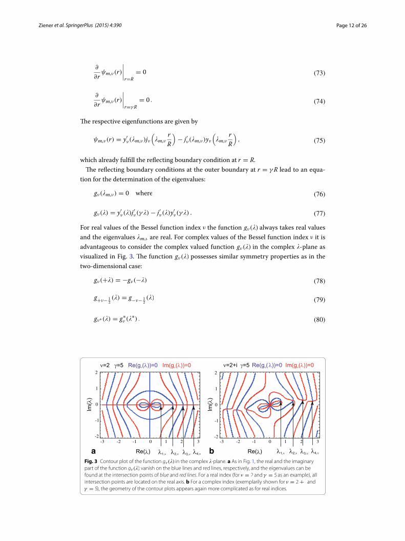
For real values of the Bessel function index ν the function gν(�) always takes real values and the eigenvalues �m,ν are real. For complex values of the Bessel function index ν it is advantageous to consider the complex valued function gν(�) in the complex �-plane as visualized in Fig. 3. The function gν(�) possesses similar symmetry properties as in the two-dimensional case:
(73)∂
∂rψm,ν(r)
∣
∣
∣
∣
r=R
= 0
(74)∂
∂rψm,ν(r)
∣
∣
∣
∣
r=γR
= 0 .
(75)ψm,ν(r) = y′ν(�m,ν)jν
(
�m,νr
R
)
− j′ν(�m,ν)yν
(
�m,νr
R
)
,
(76)gν(�m,ν) = 0 where
(77)gν(�) = y′ν(�)j′
ν(γ �)− j′ν(�)y′
ν(γ �) .
(78)gν(+�) = −gν(−�)
(79)g+ν− 1
2(�) = g
−ν− 12(�)
(80)gν∗(�) = g∗ν (�∗) .
-3 -2 -1 0 1 2 3-2
-1
0
1
2
Im(λ
)
Re(λ)
ν=2 γ=5 Re(g (λ))=0 Im(g (λ))=0
-3 -2 -1 0 1 2 3-2
-1
0
1
2
Im(λ
)
Re(λ)
ν=2+i γ=5 Re(g (λ))=0 Im(g (λ))=0ν ν ν ν
a b λ1,ν λ2,ν λ3,ν λ4,νλ1,ν λ2,ν λ3,ν λ4,ν
Fig. 3 Contour plot of the function gν(�) in the complex �-plane. a As in Fig. 1, the real and the imaginary part of the function gν(�) vanish on the blue lines and red lines, respectively, and the eigenvalues can be found at the intersection points of blue and red lines. For a real index (for ν = 2 and γ = 5 as an example), all intersection points are located on the real axis. b For a complex index (exemplarily shown for ν = 2+ i and γ = 5), the geometry of the contour plots appears again more complicated as for real indices.
Page 13 of 26Ziener et al. SpringerPlus (2015) 4:390
This translates to the symmetry properties to eigenvalues
and eigenfunctions
For small values of the parameter �, the function gν(�) given in Eq. (77) can be approxi-mated by
and, thus, the first eigenvalue can be found at
In the limit γ → 1, the first eigenvalue tends to
For small values of the index ν, the approximate value of first eigenvalue from Eq. (87) can be approximated further through a Taylor expansion:
In the same limit for small values of the parameter γ, Grebenkov found [see Eq. (34) in Grebenkov (2007)]:
and Gottlieb obtained [see Eq. (2.14) in Gottlieb (1985) or Eq. (A.10) in Gottlieb (1985)]:
(81)�m,+ν− 12= �m,−ν− 1
2
(82)�m,ν∗ = �∗
m,ν
(83)ψm,+ν− 12(r) = ψm,−ν− 1
2(r)
(84)ψm,ν∗(r) = ψ∗
m,ν(r) .
(85)gν(�) =ν
�3
ν + 1
2ν + 1
γ 2ν+1− 1
γ 2+ν
(86)+
[
2ν3 + 5ν2 + ν − 2][
1− γ 2ν+3]
+ νγ 2[
2ν2 + ν − 3][
γ 2ν−1− 1
]
2�[2ν + 1][4ν2 + 4ν − 3]γ 2+ν
(87)�1,ν ≈
√
2ν[ν + 1][
4ν2 + 4ν − 3][
1− γ 2ν+1]
[
2ν3 + 5ν2 + ν − 2][
1− γ 2ν+3]
+ νγ 2[
2ν2 + ν − 3][
γ 2ν−1 − 1] .
(88)limγ→1
�1,ν =
√
ν[1+ ν] .
(89)�1,ν ≈
√
3ν
1+ γ + γ 2.
(90)
�1,ν ≈
√
ν[1+ ν]
√
2− γ +2
3[1− γ ]2 +
1
3[1− γ ]3 −
3ν[1+ ν] − 10
90[1− γ ]4
(91)
�1,ν ≈
√
ν[1+ ν]
[
1−1
2[γ − 1] +
5
24[γ − 1]
2−
1
16[γ − 1]
3
+5− 32ν[ν + 1]
1920[γ − 1]
4
]
.
Page 14 of 26Ziener et al. SpringerPlus (2015) 4:390
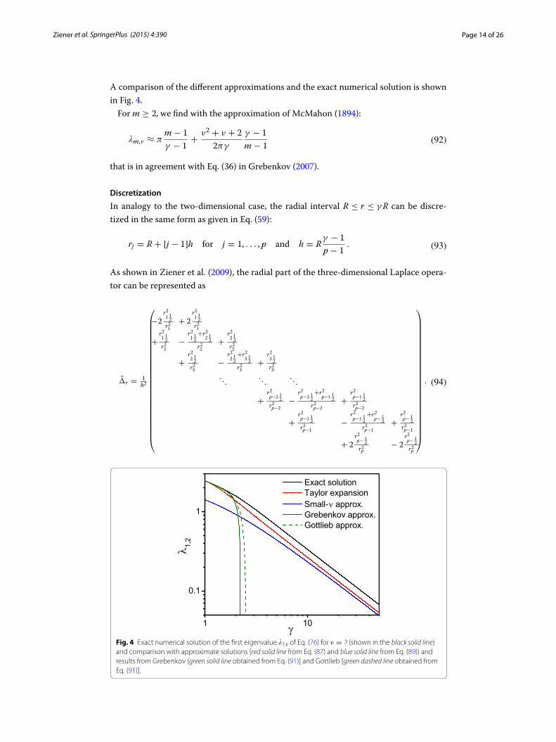
A comparison of the different approximations and the exact numerical solution is shown in Fig. 4.
For m ≥ 2, we find with the approximation of McMahon (1894):
that is in agreement with Eq. (36) in Grebenkov (2007).
Discretization
In analogy to the two-dimensional case, the radial interval R ≤ r ≤ γR can be discre-tized in the same form as given in Eq. (59):
As shown in Ziener et al. (2009), the radial part of the three-dimensional Laplace opera-tor can be represented as
(92)�m,ν ≈ πm− 1
γ − 1+
ν2 + ν + 2
2πγ
γ − 1
m− 1
(93)rj = R+ [j − 1]h for j = 1, . . . , p and h = Rγ − 1
p− 1.
(94)�̂r =1
h2
−2
r2112
r21
+ 2
r2112
r21
+
r2112
r22
−
r2112
+r2212
r22
+
r2212
r22
+
r2212
r23
−
r2212
+r2312
r23
+
r2312
r23
. . .. . .
. . .
+
r2p−2
12
r2p−2
−
r2p−2
12
+r2p−1
12
r2p−2
+
r2p−1
12
r2p−2
+
r2p−1
12
r2p−1
−
r2p−1
12
+r2p− 1
2
r2p−1
+
r2p− 1
2
r2p−1
+ 2
r2p− 1
2
r2p− 2
r2p− 1
2
r2p
.
Fig. 4 Exact numerical solution of the first eigenvalue �1,ν of Eq. (76) for ν = 2 (shown in the black solid line) and comparison with approximate solutions [red solid line from Eq. (87) and blue solid line from Eq. (89)) and results from Grebenkov (green solid line obtained from Eq. (91)] and Gottlieb [green dashed line obtained from Eq. (91)].
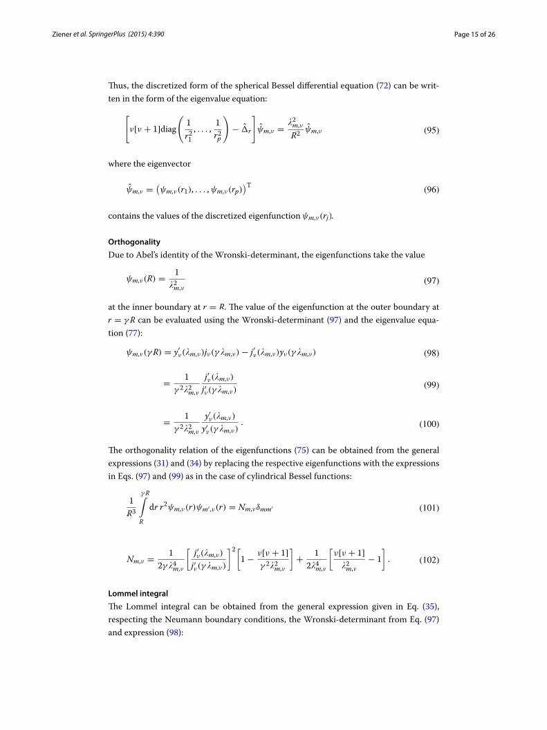
Page 15 of 26Ziener et al. SpringerPlus (2015) 4:390
Thus, the discretized form of the spherical Bessel differential equation (72) can be writ-ten in the form of the eigenvalue equation:
where the eigenvector
contains the values of the discretized eigenfunction ψm,ν(rj).
Orthogonality
Due to Abel’s identity of the Wronski-determinant, the eigenfunctions take the value
at the inner boundary at r = R. The value of the eigenfunction at the outer boundary at r = γR can be evaluated using the Wronski-determinant (97) and the eigenvalue equa-tion (77):
The orthogonality relation of the eigenfunctions (75) can be obtained from the general expressions (31) and (34) by replacing the respective eigenfunctions with the expressions in Eqs. (97) and (99) as in the case of cylindrical Bessel functions:
Lommel integral
The Lommel integral can be obtained from the general expression given in Eq. (35), respecting the Neumann boundary conditions, the Wronski-determinant from Eq. (97) and expression (98):
(95)
[
ν[ν + 1]diag
(
1
r21, . . . ,
1
r2p
)
− �̂r
]
ψ̂m,ν =�2m,ν
R2ψ̂m,ν
(96)ψ̂m,ν =(
ψm,ν(r1), . . . ,ψm,ν(rp))T
(97)ψm,ν(R) =1
�2m,ν
(98)ψm,ν(γR) = y′ν(�m,ν)jν(γ �m,ν)− j′ν(�m,ν)yν(γ �m,ν)
(99)=1
γ 2�2m,ν
j′ν(�m,ν)
j′ν(γ �m,ν)
(100)=1
γ 2�2m,ν
y′ν(�m,ν)
y′ν(γ �m,ν).
(101)1
R3
γR∫
R
dr r2ψm,ν(r)ψm′,ν(r) = Nm,νδmm′
(102)Nm,ν =1
2γ �4m,ν
[
j′ν(�m,ν)
j′ν(γ �m,ν)
]2[
1−ν[ν + 1]
γ 2�2m,ν
]
+1
2�4m,ν
[
ν[ν + 1]
�2m,ν
− 1
]
.
Page 16 of 26Ziener et al. SpringerPlus (2015) 4:390
For α + ν = 2p+ 1, the Lommel functions can be expressed in terms of Gegenbauer polynomials as above [see Eq. (22)].
In analogy to Eq. (70), the special case for α = 2 and ν = 0 can be determined, since in this case the prefactors of the Lommel functions in Eq. (103) vanish:
Therefore, the functions 1 and ψm,0(r) are orthogonal. In analogy to the cylindrical case in Eq. (71) this result can be generalized by integrating the original spherical Bessel dif-ferential equation (72)
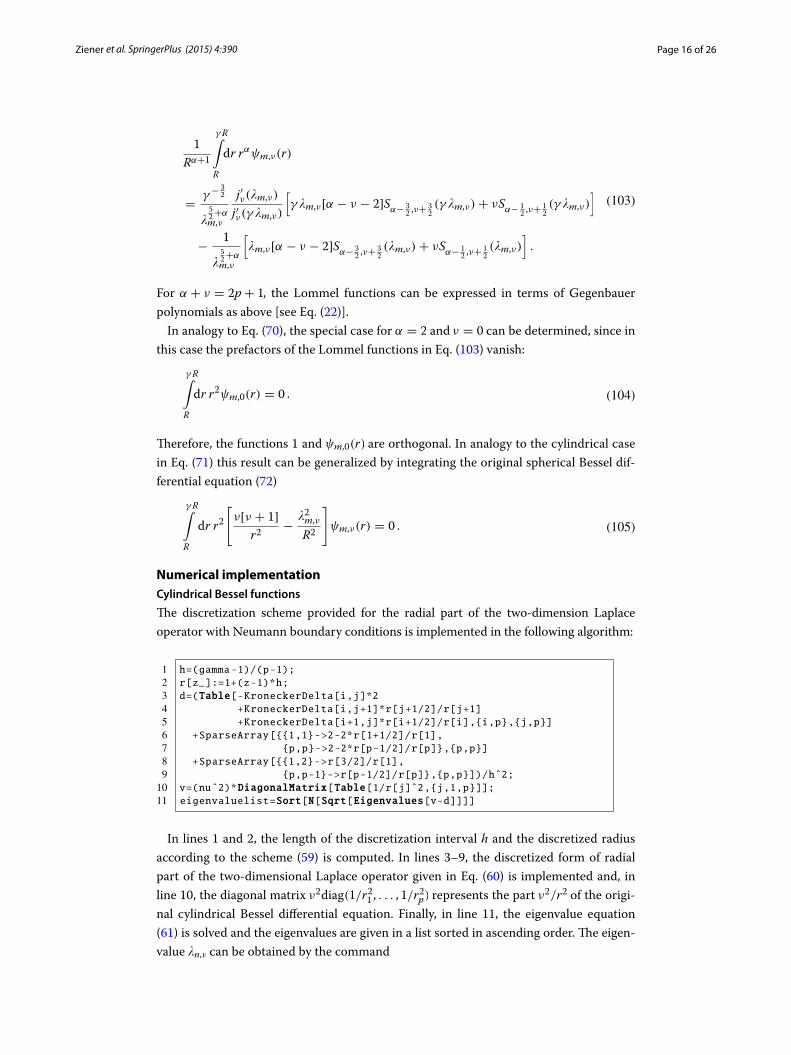
Numerical implementationCylindrical Bessel functions
The discretization scheme provided for the radial part of the two-dimension Laplace operator with Neumann boundary conditions is implemented in the following algorithm:
In lines 1 and 2, the length of the discretization interval h and the discretized radius according to the scheme (59) is computed. In lines 3–9, the discretized form of radial part of the two-dimensional Laplace operator given in Eq. (60) is implemented and, in line 10, the diagonal matrix ν2diag(1/r21 , . . . , 1/r
2p) represents the part ν2/r2 of the origi-
nal cylindrical Bessel differential equation. Finally, in line 11, the eigenvalue equation (61) is solved and the eigenvalues are given in a list sorted in ascending order. The eigen-value �n,ν can be obtained by the command
(103)
1
Rα+1
γR∫
R
dr rαψm,ν(r)
=γ−
32
�
52+αm,ν
j′ν(�m,ν)
j′ν(γ �m,ν)
[
γ �m,ν[α − ν − 2]Sα− 3
2 ,ν+32(γ �m,ν)+ νS
α− 12 ,ν+
12(γ �m,ν)
]
−1
�
52+αm,ν
[
�m,ν[α − ν − 2]Sα− 3
2 ,ν+32(�m,ν)+ νS
α− 12 ,ν+
12(�m,ν)
]
.
(104)
γR∫
R
dr r2ψm,0(r) = 0 .
(105)
γR∫
R
dr r2
[
ν[ν + 1]
r2−
�2m,ν
R2
]
ψm,ν(r) = 0 .
Page 17 of 26Ziener et al. SpringerPlus (2015) 4:390
Spherical Bessel functions
In analogy to the implementation for cylindrical Bessel functions, the eigenvalues of the radial part of the three-dimensional discretization scheme according to Eq. (94) and (95) can be implemented as follows:
Finally, the eigenvalue �m,ν of the matrix eigenvalue problem (95) can be obtained by the command
Application to the diffusion process around dipole fieldsTo visualize the applicability of the results obtained in the previous sections, the fre-quency autocorrelation function of diffusing spins with the local resonance frequency
is considered as an example. The function f (r) describes the shape of the local resonance frequency and δω its strength. The same analysis has already been performed in Ziener et al. (2008) for the diffusion between two concentric cylinders (two-dimensional case) and between two concentric spheres (three-dimensional case). The frequency autocorre-lation function can be used to analyze magnetic resonance pulse sequences and to deter-mine properties of red blood cells as shown in Ziener et al. (2010).
However, using the explicit expressions for the normalization and the Lommel inte-gral for linear combinations of cylindrical or spherical Bessel functions, respectively, it is possible to obtain considerably simpler expressions as will be demonstrated below.
The frequency autocorrelation function for spins diffusing in the volume V is defined as (Ziener et al. 2006)
(106)ω(r) = δωf (r)
(107)K (t) = δω2
∫
d3r
∫
d3r0f (r)p(r, r0, t)f (r0)p(r0)
(108)=δω2
V
∫
d3r
∫
d3r0f (r)p(r, r0, t)f (r0)
Page 18 of 26Ziener et al. SpringerPlus (2015) 4:390
where p(r, r0, t) is the probability of a spin to diffuse during the time span t from the position r0 to the position r and p(r0) = 1/V is the probability of finding a spin at posi-tion r0. This transition probability is a solution of the diffusion equation
where D is the diffusion coefficient inside the volume V in which the diffusion occurs (Bauer et al. 2005). The transition probability p(r, r0, t) can be expressed in terms of an eigenfunction expansion
with eigenvalues κl and eigenfunctions φl that fulfil the orthogonality condition
and are solutions of the eigenvalue equation
with R being the radius of the inner cylinder or the inner sphere, respectively. The eigenfunction
corresponds to the lowest eigenvalue
Cylinders
In the two-dimensional case, the diffusion occurs in the space between two concentric circles with radius R and γR:
The eigenfunctions of the eigenvalue equation (112) are
(109)∂
∂tp(r, r0, t) = D�p(r, r0, t)
(110)p(r, r0, t) =
∞∑
κl≥0
e−κ2l
Dt
R2 φl(r)φ∗
l (r0) =1
V+
∞∑
κl>0
e−κ2l
Dt
R2 φl(r)φ∗
l (r0)
(111)
∫
d3rφl(r)φ∗
l′(r) = δll′
(112)�φl(r) = −κ2l
R2φl(r) ,
(113)φ0(r) =1
√V
(114)κ0 = 0 .
(115)V = πR2[
γ 2− 1
]
.
(116)φn,ν(r,φ) =�n,ν(r)
R√
Nn,ν
e+iνφ
√2π
(117)n = +1, . . . ,+∞
(118)ν = −∞, . . . ,−1, 0,+1, . . . ,+∞ ,
Page 19 of 26Ziener et al. SpringerPlus (2015) 4:390
with the radial eigenfunctions �n,ν(r) given in Eq. (39) and the according nor-malization constants Nn,ν given in Eq. (67) where the index ν takes the values ν = −∞, . . . ,−1, 0,+1, . . . ,+∞ and the index n lies in the range n = +1, . . . ,+∞. Using the symmetry relation of the radial eigenvalues in Eq. (45) and radial eigenfunc-tions in Eq. (47), the propagator from Eq. (110) can finally be written in the form
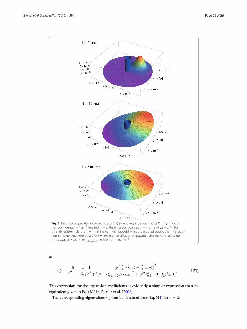
In Fig. 5 the time evolution of this diffusion propagator is visualized.Introducing the diffusion propagator and the shape-function of the two-dimensional
dipole field
into the definition of the autocorrelation function given in Eq. (108), only the addend with the index ν = 2 remains and the autocorrelation function can finally be written in the form
with the expansion coefficients
A similar expression appears in Eq. (28) in Ziener et al. (2008) for the calculation of the expansion coefficients. The Lommel integral in Eq. (122) can be evaluated by using the general expression given in Eq. (69) with α = −1 and ν = 2. In this special case the Lom-mel function can be expressed in terms of Schläfli polynomials [see Eq. (17) with m = 1 and Eq. (21)]: S−1,2(z) = S2(z)/4 = 1/z2, and, thus S′
−1,2(z) = −2/z3. Thus, one obtains:
Finally, with the normalization constant given in Eq. (67), the expansion coefficient Fn can be written as
(119)
p(r,φ, r0,φ0, t) =1
πR2[
γ 2 − 1]
+1
2πR2
∞∑
n=1
∞∑
ν=0
e−�
2n,ν
Dt
R2
Nn,ν�n,ν(r)�n,ν(r0)[2− δν0] cos(ν[φ − φ0]) .
(120)f (r,φ) =R2
r2cos(2φ)
(121)K (t) = δω2∞∑
n=1
F2ne
−�2n,2
Dt
R2
(122)Fn =1
√
γ 2 − 1
1√
Nn,2
γR∫
R
dr�n,2(r)
r.
(123)Fn =1
√
γ 2 − 1
1√
Nn,2
4
π�3n,2
[
1−1
γ 3
J ′2(�n,2)
J ′2(γ �n,2)
]
.
(124)F2n =
8
γ 2 − 1
1
�n,2
[
1− 1γ 3
J ′2(�n,2)
J ′2(γ �n,2)
]2
4 − �2n,2 +
[
�2n,2 −
4γ 2
][
J ′2(�n,2)
J ′2(γ �n,2)
]2
Page 20 of 26Ziener et al. SpringerPlus (2015) 4:390
or
This expression for the expansion coefficients is evidently a simpler expression than its equivalent given in Eq. (B1) in Ziener et al. (2008).
The corresponding eigenvalues �n,2 can be obtained from Eq. (41) for ν = 2:
(125)F2n =
8
γ 2 − 1
1
�2n,2
1
γ 4
[
γ 3J ′2(γ �n,2)− J ′2(�n,2)]2
γ 2[
4 − �2n,2
][
J ′2(γ �n,2)]2
+[
γ 2�2n,2 − 4
][
J ′2(�n,2)]2
.
Fig. 5 Diffusion propagator according to Eq. (119) around a cylinder with radius R = 1µm, diffu-sion coefficient D = 1µm2/ms and γ = 8. The initial position is at r0 = 4µm and φ0 = π/4. For small times (exemplary for t = 1ms) the transition probability is concentrated around the initial posi-tion. For large times (exemplary for t = 100ms) the diffusion propagator takes the constant value limt→∞ p(r ,φ, r0,φ0, t) =
1
πR2[γ 2−1]= 5.05254× 10⁹ m−2.
Page 21 of 26Ziener et al. SpringerPlus (2015) 4:390
and the following sums can be used to check if a sufficient numerical accuracy is obtained:
Spheres
In the three-dimensional case the diffusion occurs between two concentric spheres, and, thus, the diffusion volume corresponds to
The orthogonal eigenfunctions of the eigenvalue equation (112) are
with the radial eigenfunctions ψm,ν(r) given in Eq. (75), the respective normalization constants Nm,ν are given in Eq. (102) and the spherical harmonics are defined by
where Pµν denote the associated Legendre polynomials which are defined for the nega-
tive upper index as
(126)Y ′
2(�n,2)J′
2(γ �n,2) = J ′2(�n,2)Y′
2(γ �n,2) ,
(127)
∞∑
n=1
F2n =
1
2γ 2
(128)
∞∑
n=1
F2n�
2n,2 = 2
1+ γ 2
γ 4
(129)
∞∑
n=1
F2n
�2n,2
=ln(γ )
4[γ 2 − 1]
(130)
∞∑
n=1
F2n
�4n,2
=1
32.
(131)V =4
3πR3
[
γ 3− 1
]
.
(132)φm,ν,µ(r, θ ,φ) =ψm,ν(r)√
R3Nm,ν
Yν,µ(θ ,φ)
(133)m = +1, . . . ,+∞
(134)ν = 0,+1, . . . ,+∞
(135)µ = −ν, . . . , 0, . . . ,+ν ,
(136)Yν,µ(θ ,φ) =
√
2ν + 1
4π
[ν − µ]!
[ν + µ]!Pµν (cos(θ))e
iµφ ,
(137)P−µν (cos(θ)) = [−1]µ
[ν − µ]!
[ν + µ]!Pµν (cos(θ)) .
Page 22 of 26Ziener et al. SpringerPlus (2015) 4:390
In contradiction to the two-dimensional case, the index ν in the three-dimensional case is in the range ν = 0,+1, . . . ,+∞. The index µ takes the values µ = −ν, . . . , 0, . . . ,+ν. Therefore, the propagator given in Eq. (110) can be written as
The sum over the index µ can further be simplified by using the explicit expression of the spherical harmonics given in Eq. (136) and the definition of the associated Legendre polynomials with a negative upper index from Eq. (137):
Evidently, the transition probability p(r, θ ,φ, r0, θ0,φ0, t) to go in time t from position (r0, θ0,φ0) to position (r, θ ,φ) depends on the radial distances r0 and r and the spherical angle � = (θ0,φ0; θ ,φ) that can be determined by the spherical law of cosines:
Using the addition theorem for spherical harmonics [see 14.30.9 in Olver et al. (2010)]
the transition probability can finally be written in the form
Comparing the addition theorem for spherical harmonics in Eq. (141) with the sum over the product of the spherical harmonics in Eq. (139), the results of Eq. (10) on page 382 of section 14.16. I. in Carslaw and Jaeger (1959) can be reproduced.
The three-dimensional dipole field has the shape
(138)
p(r, θ ,φ, r0, θ0,φ0, t) =3
4πR3[
γ 3 − 1]
+1
R3
∞∑
m=1
∞∑
ν=0
+ν∑
µ=−ν
e−�2m,ν
Dt
R2
Nm,ν
ψm,ν(r)ψm,ν(r0)Yν,µ(θ ,φ)Y∗
ν,µ(θ0,φ0) .
(139)
+ν∑
µ=−ν
Yν,µ(θ ,φ)Y∗
ν,µ(θ0,φ0) =2ν + 1
4πPν(cos(θ))Pν(cos(θ0))
+2ν + 1
2π
+ν∑
µ=+1
[ν − µ]!
[ν + µ]!Pµν (cos(θ))P
µν (cos(θ0)) cos (µ[φ − φ0])
=2ν + 1
4π
+ν∑
µ=0
[ν − µ]!
[ν + µ]!Pµν (cos(θ))P
µν (cos(θ0))[2− δµ0] cos (µ[φ − φ0]) .
(140)cos(�) = cos(θ0) cos(θ)+ sin(θ0) sin(θ) cos(φ0 − φ) .
(141)
+ν∑
µ=−ν
Yν,µ(θ ,φ)Y∗
ν,µ(θ0,φ0) =2ν + 1
4πPν(cos(θ0) cos(θ)+ sin(θ0) sin(θ) cos(φ0 − φ))
=2ν + 1
4πPν(cos(�))
(142)
p(r, r0,�, t) =1
4πR3
[
3
γ 3 − 1+
∞∑
m=1
∞∑
ν=0
2ν + 1
Nm,ν
e−�
2m,ν
Dt
R2 ψm,ν(r)ψm,ν(r0)Pν(cos(�))
]
.
(143)f (r, θ ,φ) =R3
r3
[
3 cos2(θ)− 1]
= 4
√
π
5Y20(θ ,φ)
R3
r3.
Page 23 of 26Ziener et al. SpringerPlus (2015) 4:390
Introducing this shape function and the three-dimensional propagator from Eq. (138) into the definition of the autocorrelation function (108), leads to
with the expansion coefficients
The remaining Lommel integral can be solved by using the expression (103) for α = −1 and ν = 2. The occurring Lommel functions S
−52 ,+
72(z) and S
−32 ,+
52(z) can explicitly be
given by using the relation (22):
where A0, 72(z) and A0, 52
(z) can be obtained from Eq. (25). Thus, the integration yields:
Introducing the normalization constant from Eq. (102) yields:
For ν = 2 the spherical Bessel functions can be expressed in terms of the sine and cosine function:
(144)K (t) = δω2∞∑
m=1
F2me
−�2m,2
Dt
R2
(145)
Fm =
√
3
4πR3[
γ 3 − 1]
π∫
0
dθ
2π∫
0
dφ
γR∫
R
dr r2 sin(θ)4
√
π
5Y20(θ ,φ)
R3
r3Y20(θ ,φ)√
R3Nm,2
ψm,2(r)
(146)=1
√
γ 3 − 1
√
3
5
2√
Nm,2
γR∫
R
drψm,2(r)
r.
(147)S−
52 ,+
72(z) =
2
7
z−52
272Ŵ( 72 )
A0, 72(z) = z−
72
(148)S−
32 ,+
52(z) =
2
5
z−32
252Ŵ( 52 )
A0, 52(z) = z−
52
(149)Fm =1
√
γ 3 − 1
√
3
5
6√
Nm,2
1
�4m,2
[
1−1
γ 4
j′2(�m,2)
j′2(γ �m,2)
]
.
(150)F2m =
216
5
1
�2m,2
1
γ 3 − 1
[
1− 1γ 4
j′2(�m,2)
j′2(γ �m,2)
]2
γ 2�2m,2−6
γ 3
[
j′2(�m,2)
j′2(γ �m,2)
]2+ 6− �
2m,2
.
(151)j2(z) =
[
3
z3−
1
z
]
sin(z)−3
z2cos(z)
(152)y2(z) = −
[
3
z3−
1
z
]
cos(z)−3
z2sin(z)
Page 24 of 26Ziener et al. SpringerPlus (2015) 4:390
which will be necessary for further simplifications. The derivative of the spherical Bessel functions can be simplified by using the relation (151):
Finally, the expansion coefficients can be written as
or in the form
This expression for the expansion coefficients is much more simpler than the equivalent expression given in Eq. (B4) in Ziener et al. (2008) or in Eq. (7) in Ziener et al. (2010).
The eigenvalues can be obtained from Eq. (77) for ν = 2, which can be further simpli-fied using the expressions (151) and (152). Finally, the following transcendental equation has to be solved:
This equation coincides with Eq. (5) in Kurz et al. (2014) for �m,2 =√κ and γ = η−1/3.
The following sums can be used to check if a sufficient numerical accuracy is obtained:
(153)j′2(�m,2)
j′2(γ �m,2)= γ 4
[4�2m,2 − 9] sin(�m,2)+ �m,2[9− �2m,2] cos(�m,2)
[4γ 2�2m,2 − 9] sin(γ �m,2)+ γ �m,2[9− γ 2�
2m,2] cos(γ �m,2)
.
(154)
F2m =
216
5
1
�2m,2
1
γ 3 − 1
[
1−[4�2m,2
−9] sin(�m,2)+�m,2[9−�2m,2
] cos(�m,2)
[4γ 2�2m,2
−9] sin(γ �m,2)+γ �m,2[9−γ 2�2m,2
] cos(γ �m,2)
]2
γ 5
[
[4�2m,2−9] sin(�m,2)+�m,2[9−�
2m,2
] cos(�m,2)
[4γ 2�2m,2
−9] sin(γ �m,2)+γ �m,2[9−γ 2�2m,2
] cos(γ �m,2)
]2[
γ 2�2m,2
− 6]
+ 6− �2m,2
(155)
F2m =
2165
1
�2m,2
1
γ 3−1
×
[
[4γ 2�2m,2
−9] sin(γ �m,2)+γ �m,2[9−γ 2�2m,2
] cos(γ �m,2)−[4�2m,2−9] sin(�m,2)−�m,2[9−�
2m,2
] cos(�m,2)
]2
γ 5
[
[4�2m,2−9] sin(�m,2)+�m,2[9−�
2m,2
] cos(�m,2)
]2
[γ 2�2m,2
−6]+[6−�2m,2
]
[
[4γ 2�2m,2
−9] sin(γ �m,2)+γ �m,2[9−γ 2�2m,2
] cos(γ �m,2)
]2 .
(156)
tan(�m,2[γ − 1])
�m,2[γ − 1]=
81− 9�2m,2[γ2− 3γ + 1] + 4γ 2
�4m,2
81− 9�2m,2[4γ2 − 9γ + 4] + γ �4m,2[16γ − 9γ 2 − 9] + γ 3�
6m,2
.
(157)
∞∑
m=1
F2m =
4
5γ 3
(158)
∞∑
m=1
F2m�
2m,2 =
36
5γ 5
γ 5− 1
γ 3 − 1
(159)
∞∑
m=1
F2m
�2m,2
=2
5
1
γ 3 − 1
[
1−1
γ+
4[γ 3− 1]2 + 9γ [2γ 2
− 1− γ 4]
36γ [1− γ 5]
]
.
Page 25 of 26Ziener et al. SpringerPlus (2015) 4:390
Summary and conclusionsCylindrical and spherical Bessel functions are frequently employed in treating bound-ary value and eigenvalue problems in applied mathematics (Gray and Mathews 1895; McLachlan 1941; Kac 1966). In this work, the general orthogonality relation and Lommel integral of a linear combination of both cylindrical and spherical Bessel functions, respec-tively, are considered. For a given radius interval of R ≤ r ≤ γR, Neumann boundary con-ditions are assumed and the corresponding approximated first eigenvalues �1,ν for small � and ν are compared in their γ-dependency with expressions from the literature in the same limit and the exact numerical solution for cylindrical and spherical Bessel functions, respectively (see Figs. 3, 4). It is shown that all expressions agree well for γ → 1. Conse-quently, explicit terms for the orthogonality relation, normalization constant and Lommel integral are given in both model geometries using a discretized form of the respective Bessel differential equations. In the case of spherical Bessel functions, these results are a generalization from integer indices, that can be presented in terms of trigonometric func-tions and have so mostly to treat related physical problems (Carslaw and Jaeger 1959), to arbitrary complex-valued indices. Moreover, a numerical implementation to calculate the relevant eigenvalues is provided and the results are applied to a scenario in magnetic resonance physics where spin diffusion processes between two magnetic concentric cyl-inders or two concentric spheres occur. Thereby, an eigenfunction expansion of the spin transition probability function results in analytic expressions for the expansion coef-ficients of the frequency autocorrelation function K(t). These are mathematically easier to grasp and, therefore, to implement numerically, than equivalent expressions that have been derived recently (Ziener et al. 2008). The results might be useful to obtain analyti-cal expressions for the transverse relaxation in Carr-Purcell-Meiboom-Gill experiments where Jensen and Chandra have provided a relation between the diffusion-dependent part of transverse relaxation and the frequency autocorrelation function within a weak field approximation (Jensen et al. 2001; Jensen and Chandra 2000). With the paramag-netic properties of deoxygenated hemoglobin, such analyses may then be applied to study highly organized (cylindriform) capillary arrangements in, for instance, skeletal muscle tissue (Ziener et al. 2012). Likewise, the results for spherical geometries may be used to quantify microstructural parameters in lung tissue by treating lung alveoli as spherical entities that are surrounded by a dense capillary network. A further analysis might con-sider mixed boundary conditions and/or extend the results to other model geometries.
Authors’ contributions This work was carried out by the four authors, in collaboration. CHZ designed research; CHZ, FTK, LRB, and TK performed research; CHZ contributed numerical tools; CHZ, FTK. and TK analyzed data; and CHZ, FTK and TK wrote the paper. All authors read and approved the final manuscript.
Author details1 Department of Radiology, German Cancer Research Center-DKFZ, Im Neuenheimer Feld 280, 69120 Heidelberg, Germany. 2 Division of Neuroradiology, Heidelberg University, Im Neuenheimer Feld 400, 69120 Heidelberg, Germany. 3 Department of Experimental Physics 5, University of Würzburg, Am Hubland, 97074 Würzburg, Germany.
AcknowledgementsThis work was supported by grants from the Deutsche Forschungsgemeinschaft (Contract Grant number: DFG ZI 1295/2-1). F.T. Kurz was supported by a postdoctoral fellowship from the medical faculty of Heidelberg University.
Compliance with ethical guidelines
Competing interestsThe authors declare that they have no competing interests.
Page 26 of 26Ziener et al. SpringerPlus (2015) 4:390
Received: 4 March 2015 Accepted: 7 July 2015
ReferencesAbramowitz M, Stegun IA (1972) Handbook of mathematical functions with formulas, graphs, and mathematical tables.
Dover, New YorkBabister AW (1967) Transcendental functions satisfying nonhomogeneous linear differential equations. Macmillan,
NewYorkBauer HF (1964) Tables of zeros of cross product Bessel functions J′p(ξ)Y
′p(kξ)− J′p(kξ)Y
′p(ξ) = 0. Math Comp
18:128–135Bauer WR, Ziener CH, Jakob PM (2005) Non-Gaussian spin dephasing. Phys Rev A 71:053412Bridge JF, Angrist SW (1962) An extended table of roots of J′n(x)Y
′n(βx)− J′n(βx)Y
′n(x) = 0. Math Comp 16:198–204
Buchholz H (1949) Besondere Reihenentwicklungen für eine häufig vorkommende zweireihige Determinante mit Zylin-derfunktionen und ihre Nullstellen. Z Angew Math Mech 29:356–367
Carslaw HS, Jaeger JC (1959) Conduction of heat In solids. University Press, OxfordCochran JA (1964) Remarks on the zeros of cross-product Bessel functions. J Soc Indust Appl Math 12:580–587Cochran JA (1966a) The asymptotic nature of zeros of cross-product Bessel functions. Quart J Mech Appl Math
19:511–522Cochran JA (1966b) The analyticity of cross-product Bessel function zeros. Proc Camb Phil Soc 62:215–226Glasser ML (2010) Integral representations for the exceptional univariate Lommel functions. J Phys A Math Theor
43:155207Goodwin ET (1949) Recurrence relations for cross-products of Bessel functions. Quart J Mech Appl Math 2:72–74Gottlieb HPW (1985) Eigenvalues of the Laplacian with Neumann boundary conditions. J Austral Math Soc Ser B
26:293–309Gottlieb HPW (1985) On the exceptional zeros of cross-products of derivatives of spherical Bessel functions. Z Angew
Math Phys 36:491–494Gray A, Mathews GB (1895) A treatise on Bessel functions and their applications to physics. MacMillan, LondonGrebenkov DS (2007) Analytical solution for restricted diffusion in circular and spherical layers under inhomogeneous
magnetic fields. J Chem Phys 128:134702Jensen JH, Chandra R, Yu H (2001) Quantitative model for the interecho time dependence of the CPMG relaxation rate in
iron-rich gray matter. Magn Reson Med 46:159–165Jensen JH, Chandra R (2000) NMR relaxation in tissues with weak magnetic inhomogeneities. Magn Reson Med
44:144–156Kac M (1966) Can one hear the shape of a drum? Amer Math Monthly 73:1–23Kurz FT, Kampf T, Heiland S, Bendszus M, Schlemmer HP, Ziener CH (2014) Theoretical model of the single spin-echo
relaxation time for spherical magnetic perturbers. Magn Reson Med 71:1888–1895Laslett LJ, Lewish W (1962) Evaluation of the zeros of cross-product Bessel functions. Math Comp 16:226–232Magnus W, Oberhettinger F, Soni RP (1966) Formulas and theorems for the special functions of mathematical physics.
Springer, BerlinMcLachlan NW (1941) Bessel functions for engineers. University Press, OxfordMcMahon J (1894) On the roots of the Bessel and certain related functions. Ann Math 9:23–30Olver FWJ, Lozier DW, Boisvert RF, Clark CW (2010) NIST handbook of mathematical functions. University Press,
CambridgeSorolla E, Mosig JR, Mattes M (2013) Algorithm to calculate a large number of roots of the cross-product of Bessel func-
tions. IEEE Trans Antennas Propag 61:2180–2187Thambynayagam RKM (2011) The diffusion handbook: applied solutions for engineers. McGraw-Hill, New YorkTruell R (1943) Concerning the roots of J′ν (x)N
′ν (qx)− J′ν (qx)N
′ν (x) = 0. J Appl Phys 14:350–352
Watson GN (1966) A Treatise on the Theory of Bessel Functions. University Press, CambridgeWolfram S (1999) The Mathematica Book. Cambridge University Press, New YorkZiener CH, Bauer WR, Melkus G, Weber T, Herold V, Jakob PM (2006) Structure-specific magnetic field inhomogeneities
and its effect on the correlation time. Magn Reson Imaging 24:1341–1347Ziener CH, Kampf T, Herold V, Jakob PM, Bauer WR, Nadler W (2008) Frequency autocorrelation function of stochastically
fluctuating fields caused by specific magnetic field inhomogeneities. J Chem Phys 129:014507Ziener CH, Glutsch S, Jakob PM, Bauer WR (2009) Spin dephasing in the dipole field around capillaries and cells: numeri-
cal solution. Phys Rev E 80:046701Ziener CH, Kampf T, Jakob PM, Bauer WR (2010) Diffusion effects on the CPMG relaxation rate in a dipolar field. J Magn
Reson 202:38–42Ziener CH, Kampf T, Reents G, Schlemmer H-P, Bauer WR (2012) Spin dephasing in a magnetic dipole field. Phys Rev E
85:051908Ziener CH, Kampf T, Melkus G, Jakob PM, Schlemmer HP, Bauer WR (2012) Signal evolution in the local magnetic field of a
capillary—analogy to the damped driven harmonic oscillator. Magn Reson Imaging 30:540–553Ziener CH, Kurz FT, Kampf T (2015) Free induction decay caused by a dipole field. Phys Rev E 91:032707Ziener CH, Schlemmer HP (2013) The inverse Laplace transform of the modified Lommel functions. Integ Transf Spec F
24:141–155