Assessment of the Bill Emerson Memorial Bridge

Organizational Results Research Report September 2007 OR08.003

Prepared by University of

Missouri-Rolla and

Missouri Department

of Transportation

Assessment of the Bill Emerson Memorial Cable-stayed Bridge

Based on Seismic Instrumentation Data

FINAL REPORT

RI05-023

Prepared for Missouri Department of Transportation

Organizational Results

by University Transportation Center at the University of Missouri-Rolla

September 2007

The opinions, findings, and conclusions expressed in this publication are those of the principal investigators and the Missouri Department of Transportation; Research, Development and Technology. They are not necessarily those of the U.S. Department of Transportation, Federal Highway Administration. This report does not constitute a standard or regulation.

i

TECHNICAL REPORT DOCUMENTATION PAGE

1. Report No.

2. Government Accession No. 3. Recipient's Catalog No.

OR08-003 4. Title and Subtitle 5. Report Date Assessment of the Bill Emerson Memorial Cable-stayed Bridge Based on Seismic Instrumentation Data

September 2007 6. Performing Organization Code University of Missouri-Rolla

7. Author(s) 8. Performing Organization Report No.

G. Chen, D. Yan, W. Wang, M. Zheng, L. Ge, and F. Liu 9. Performing Organization Name and Address 10. Work Unit No. University of Missouri-Rolla 328 Butler-Carlton Civil Engineering Hall

11. Contract or Grant No.

1870 Miner Circle, Rolla, MO 65409-0030 RI05-023 12. Sponsoring Agency Name and Address 13. Type of Report and Period

Covered Missouri Department of Transportation Organizational Results P. O. Box 270-Jefferson City, MO 65102

Final Report 14. Sponsoring Agency Code MoDOT

15. Supplementary Notes This research was conducted In collaboration with the U.S. Department of Transportation through University Transportation Center at the University of Missouri-Rolla 16. Abstract

In this study, both ambient and earthquake data measured from the Bill Emerson Memorial Cable-stayed Bridge are reported and analyzed. Based on the seismic instrumentation data, the vibration characteristics of the bridge are investigated and used to validate a three-dimensional Finite Element (3-D FE) model of the bridge structure. The 3-D model is rigorous and comprehensive, representing realistic dynamic behaviors of the bridge. It takes into account the geometric nonlinear properties caused by cable sagging and soil-foundation-structure interaction in the Illinois approach of the bridge. The FE model is successfully verified and validated by using the natural frequencies and mode shapes of the bridge extracted from the measured data. With the calibrated model, time history analyses were performed to assess the condition of the bridge structure under a postulated design earthquake. Since the FE model is developed according to as-built drawings, the calibrated model can be used as a benchmark for safety evaluation and health monitoring of the cable-stayed bridge in the future. 17. Key Words 18. Distribution Statement Cable-stayed bridge; finite element model; modal analysis; cable sagging effect; seismic excitation 19. Security Classification 20. Security Classification 21. No. of Pages 22. Price

Unclassified Unclassified 119

ii

ACKNOWLEDGMENTS

The authors would like to express their deepest gratitude to continuing coordination and support by Bryan Hartnagel, Ph.D., P.E., Structural Hydraulics Engineer, Jefferson City, and his assistance over the duration of the project. Financial support to complete this study was provided in part by the Missouri Transportation Institute/Missouri Department of Transportation and by the U.S. Department of Transportation under the auspices of University Transportation Center at the University of Missouri-Rolla.

iii

Executive Summary Open to traffic on December 13, 2003, the Bill Emerson Memorial Bridge is a 1206 m (3956 ft) long cable-stayed structure. It carries four lanes of vehicular traffic along Missouri State Highway 34, Missouri State Highway 74 and Illinois Route 146 across the Mississippi River between Cape Girardeau, Missouri, and East Cape Girardeau, Illinois. The structure consists of 128 cables, two longitudinal stiffened steel girders, and two towers in the cable-stayed spans, and 12 additional piers in the Illinois approach span. In addition to four pot bearings at two towers, the superstructure of the cable-stayed span is constrained to the substructure with 16 longitudinal earthquake shock transfer devices at two towers, four tie-down devices at two ends of the cable-stayed span, and six lateral earthquake restrainers. The approach span is composed of one simply-supported, one four-span continuous, and two three-span continuous steel girder structures.

Seismic instrumentation system The Missouri end of the bridge directly rests on rock and the Illinois end is supported on drilled shaft foundations. Due to its complexity in structure and site geology as well as its proximity to the New Madrid Seismic Zone, the bridge was instrumented with an 84-accelerometer, real-time, seismic instrumentation system. The monitoring system has been in operation since December 2004 and it continuously records site and structural responses due to traffic loading and minor earthquakes. However, only a most recent 16-day worth of recorded data are kept on file unless a sizable earthquake has been identified.

At 12:37′32″ (Universal Time) of May 1, 2005, an earthquake of M4.1 on a Richter scale occurred at four miles SSE (162o) from Manila, Arkansas, and 180 kilometers from the bridge. The hypocenter depth was estimated to be about 10 kilometers. This set of earthquake data will be used to validate a three-dimensional finite element (3-D FE) model of the cable-stayed bridge.

Research objectives The objectives of this study are to retrieve peak ground and structure accelerations from the real-time instrumentation system, assess the condition of the bridge structure under a design earthquake, develop and validate a 3-D FE model that represents the actual behavior of the bridge.

To achieve the above objectives, several topics are studied in this report, including: (1) automatic retrieval of peak accelerations and measured data analysis, (2) 3-D FE bridge model with explicit modeling of all main components, (3) sensitivity study and validation of the 3-D FE bridge model, and (4) seismic behavior and assessment of the bridge structure.

iv

Conclusions and recommendations

Based on the comprehensive analysis of the cable-stayed bridge, the following conclusions can be drawn:

1. A Java-based system was developed to automatically compile the peak ground and structural accelerations measured from the bridge. The system can be seamlessly integrated with the data management system at the ISIS website. The output of this system is a string of peak acceleration data every hour or other time windows. They can be pulled into an Excel sheet for further processing.

2. The peak-picking method in frequency domain can be conveniently applied to analyze a huge set of field measured data from the seismic monitoring system. The vibration characteristics of the bridge such as natural frequencies and mode shapes were extracted.

3. Cables and bearings significantly influence the stiffness of the bridge system. The sagging of cables should be considered in the modeling of the cable-stayed bridge to account for geometric nonlinear effects. Bearings play an important role in seismic behaviors of the complex cable-stayed bridge.

4. The 3-D response and behavior of the cable-stayed bridge are evident. Most of the vibration modes are coupled with others. The dynamic characteristics (frequency and mode shapes) of the bridge indicate that the cable-stayed structure is most flexible in vertical direction and least flexible in longitudinal direction. This observation is generally supported by time history analysis.

5. The 31 significant modes of vibration up to 14.09 Hz include more than 70% mass participation in translational and rotational motions along any of three directions. The fundamental frequency is 0.339 Hz, corresponding to vertical vibration of the main bridge. Cables begin to vibrate severely at a natural frequency of 0.842 Hz or higher. The Illinois approach spans experience significant vibration at approximately 3.187 Hz. The approach spans are much stiffer than the cable-stayed span. Their interaction during earthquakes is weak.

6. Based on sensitivity analysis, the key parameters affecting the modal properties of the bridge are the mass density of concrete and boundary conditions. The mass density of concrete, specified in bridge drawings, appear underestimated by 6.7%. They need to be increased in order to match the natural frequencies of the 3-D model with their respective measured data. Except for expansion conditions, the use of other boundary conditions at bases of all piers changes the natural frequency of the main bridge by less than 5%.

7. The computed natural frequencies of the 3-D FE model agree well with those from field measured data. The maximum error of the first 31 significant modes is within 10%. For mode shapes, however, slight differences exist between the computed and the measured values due in part to unknown exact locations of all accelerometers. Nevertheless, the mode assurance criterion index between a computed mode shape and its corresponding measured one is above 0.888 for the first eight modes. This indicates that the 3-D FE model is fairly accurate for engineering applications.

v

8. All cables behave elastically under a design earthquake. Their factor of safety is larger than 2.35 at all times. On the other hand, the cable subjected to least stress is always in tension, ensuring no slack occurrence during the earthquake. Therefore, cables can be simplified as linear elements for seismic analysis.

9. The solid section of both towers at the lower portion is generally more critical than the hollow section of the upper portion above the cap beams. The in-plane behavior of two towers is always in elastic range under the design earthquake with a wide margin of safety. For out-of-plane behavior, the upper portion of the towers above the cap beams remains nearly elastic with a significant margin of safety. The lower portion of the towers, however, likely experiences moderate yielding out of plane during the design earthquake though the safety of the bridge is not a concern.

Future research The current study only addressed one way of using the recorded data for structural assessment of the bridge under a projected design earthquake. The vast arrays of acceleration data can also be used to address a number of issues related to engineering seismology, engineering design, bridge maintenance, bridge security, and bridge management. In a long term, these potential uses include, but are not limited to,

1. Assess the bridge structural condition in near real time to compliment the mandatory biennial inspections of the bridge so that the problem areas, if any, can be readily probed and examined in a cost-effective way.

2. Evaluate the bridge structural condition in a short time immediately after a catastrophic earthquake event to assist in decision making for emergency traffic uses or general public transportation in a much shorter time than traditional visual inspections may take.

3. Validate design assumptions made during the design of the cabled-stayed bridge. Several structure details are unique features to the Bill Emerson Memorial Bridge. Due to complexity and large scale of the Bridge, these unique features generally cannot be validated to the full extent with laboratory tests. The acceleration data measured from the bridge are valuable to accomplishing this important engineering task.

4. Collect the load data of small and moderate earthquakes for bridges in the Central United States and study the free field response of soil deposits and the spatial distribution of ground motions.

5. Monitor the security and safety of the critical transportation system in combination with other visual tools that may be installed in the future such as blast effects and vehicle impact.

This study provides a 3-D baseline model of the cable-stayed bridge that has been validated against the field measured traffic data and those data recorded during the May 1 2005 earthquake. This model can be applied to develop a system identification scheme for potential damage detection using emerging technologies, such as neural network, and vibration-based techniques. Further development in this direction will address the first

vi

two applications of the measured data from the above list. With strong motion data collected in the future, the 3-D model can also be expanded to fully validate design assumptions, which is the 3rd application, and to study the seismic behavior of the bridge under actual earthquakes.

vii

Table of Contents Executive summary...................................................................................................................... iv

........................................................................... x

........................................................................ xiii

........................................................................... 1

........................................................................... 1

........................................................................... 2

........................................................................... 6

........................................................................... 6

........................................................................... 7 ............................................................................. 7

List of Figure Captions......................................List of Table Captions .......................................1. Introduction............................................

1.1. General.........................................1.2. Bridge description........................1.3. Seismic instrumentation system...1.4. Scope of work ..............................1.5. Significance of this study............1.6. Organization of this report ..........

2. Automatic Retrieval of Peak Accelerations from Real-time Seismic Instrumentation System

................................................................................................................................ 9

2.1. General.................................................................................................................... 9 ............................................................... 9 ............................................................. 10 ............................................................. 10 ............................................................. 11 ............................................................. 11 ............................................................. 13 ............................................................. 15

............................................................. 16 ................................................ 16 ................................................ 17 ................................................ 19 ................................................ 19 ................................................ 21 ................................................ 22 ................................................ 26 ................................................ 26 ................................................ 27 ................................................ 28 ................................................ 38 ........

........................................................ 40

2.2. Peak acceleration retrieval .......................2.2.1. Seismograms servers......................2.2.2. Which seismogram server to use?..2.2.3. Map/Find stations...........................2.2.4. Query..............................................2.2.5. Displaying seismograms ................2.2.6. Saved data ......................................

3. Seismic Instrumentation System and Measured Data Analysis

....................................

3.1. General..................................................................3.2. Seismic instrumentation network..........................3.3. Measured data .......................................................

3.3.1. Vertical vibration of the bridge deck ..........3.3.2. Transverse vibration....................................3.3.3. Longitudinal vibration of the bridge tower.

3.4. Data analysis method ............................................3.4.1. General........................................................3.4.2. Theory of Peak-Picking method .................

3.5. Measured data analysis .........................................3.6. Mode shapes extracted from measure data ...3.7. Remarks ........................................................

4. Finite Element Modeling of Bill Emerson Memorial Cable-stayed Bridge............... 41 4.1. General.................................................................................................................. 41

.......................................................... 41 ..................................... 42 ..................................... 42 ..................................... 42 ..................................... 43 ..................................... 44

.....................

.....................

.....................

.....................

.....................

4.2. Bridge geometry..........................................

..................................... 46

4.3. Material properties ......................................4.4. Modeling of the main structural members ..

4.4.1. Towers...............................................4.4.2. Girders...............................................4.4.3. Cables................................................4.4.4. Connection bearings between towers and decks....

viii

4.4.5. Foundations in main and approach spans ........................4.5. Details of the bridge model........................................................4.6. Remarks .....................................................................................

5. Eigensolution and Model Verification of the Cable-stayed Bridge . 5.1. General.......................................................................................5.2. Modal analysis ...........................................................................

5.2.1. Classical modal analysis theory .......................................5.2.2. Modal analysis of Bill Emerson Memorial cable-stayed bridge

5.3. Parametric study..................................................................................5.3.1. Boundary condition...................................................................5.3.2. Mass density of concrete...........................................................5.3.3. Presence of the approach span of the bridge.............................5.3.4. Influence of pile foundation......................................................

5.4. Model calibration and verification......................................................5.4.1. Calibration by natural frequency ..............................................5.4.2. Mode shape verification............................................................

5.5. Remarks ..............................................................................................6. Time History Analysis and Structural Assessment of the Cable-stayed Bridge

6.1 General...........................................................................................................6.2 Time history analysis ................6.3 Evaluation of the bridge...........6.4 Remarks ....................................

7. Conclusions and Recommendations.. 7.1 Main findings ............................7.2 Future research..........................

8. References............................................ 9. Appendix a: Stiffness and damping

coefficients of bridge piers..................10. Appendix B: Unit conversion.............

........................... 46

........................... 48

........................... 51

........................... 52

........................... 52

........................... 52

........................... 52 ................. 53 .................. 63 .................. 63 .................. 65 .................. 67 .................. 68 .................. 70 .................. 71 .................. 72 .................. 76

....... 78

....... 78

....... 78

....... 84

....... 91

....... 93

....... 93

....... 94

....... 96

..... 100

..... 106

.....................................................................

.....................................................................

.....................................................................

.....................................................................

.....................................................................

.....................................................................

.....................................................................

.....................................................................

.....................................................................

ix

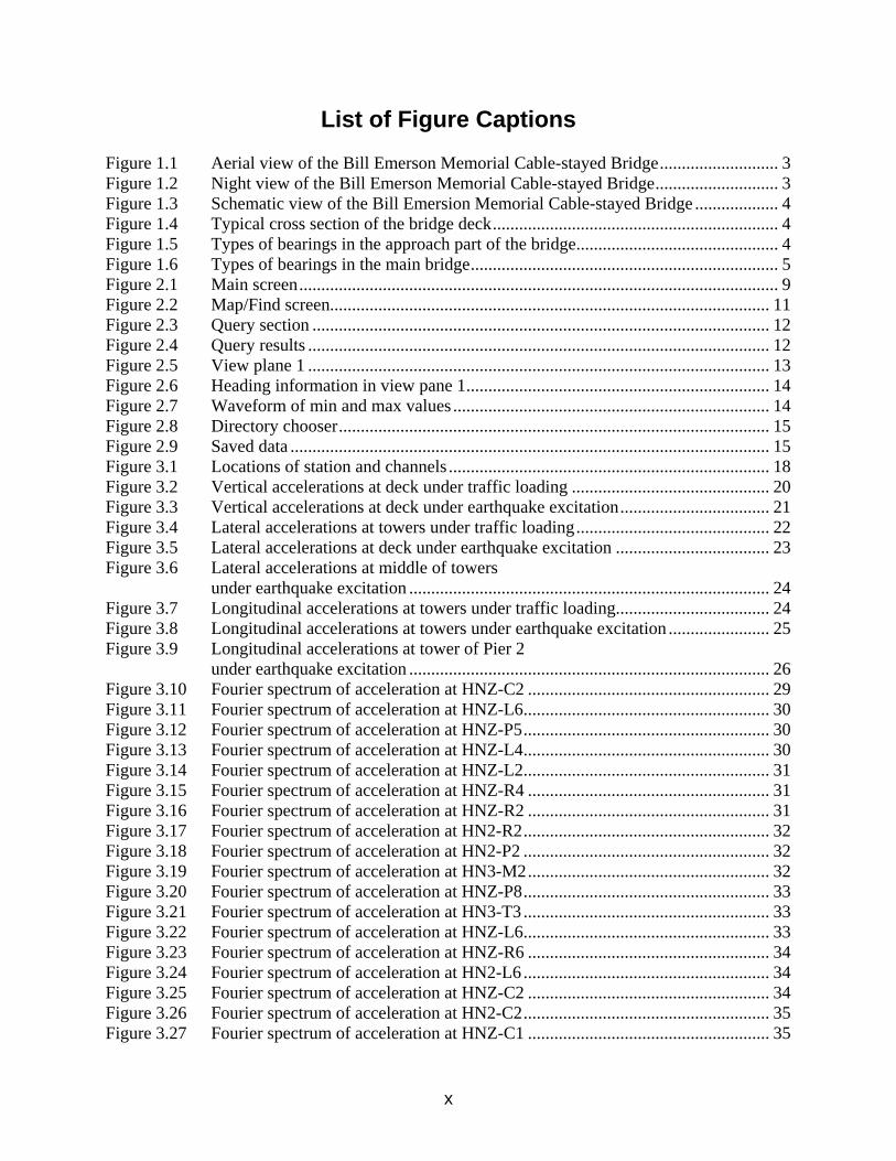
List of Figure Captions Figure 1.1 Aerial view of the Bill Emerson Memorial Cable-stayed Bridge........................... 3

.................. 3

.................. 4

.................. 4

.................. 4

.................. 5

.................. 9

................ 11

................ 12

................ 12

................ 13

................ 14

................ 14

................ 15

................ 15

................ 18

................ 20

................ 21

................ 22

................ 23

................ 24

................ 24

................ 25

................ 26

................ 29

................ 30

................ 30

................ 30

................ 31

................ 31

................ 31

................ 32

................ 32

................ 32

................ 33

................ 33

................ 33

................ 34

................ 34

................ 34

................ 35

................ 35

Figure 1.2 Night view of the Bill Emerson Memorial Cable-stayed Bridge..........Figure 1.3 Schematic view of the Bill Emersion Memorial Cable-stayed Bridge .Figure 1.4 Typical cross section of the bridge deck...............................................Figure 1.5 Types of bearings in the approach part of the bridge............................Figure 1.6 Types of bearings in the main bridge....................................................Figure 2.1 Main screen...........................................................................................Figure 2.2 Map/Find screen....................................................................................Figure 2.3 Query section ........................................................................................Figure 2.4 Query results .........................................................................................Figure 2.5 View plane 1 .........................................................................................Figure 2.6 Heading information in view pane 1.....................................................Figure 2.7 Waveform of min and max values ........................................................Figure 2.8 Directory chooser..................................................................................Figure 2.9 Saved data .............................................................................................Figure 3.1 Locations of station and channels .........................................................Figure 3.2 Vertical accelerations at deck under traffic loading .............................Figure 3.3 Vertical accelerations at deck under earthquake excitation..................Figure 3.4 Lateral accelerations at towers under traffic loading............................Figure 3.5 Lateral accelerations at deck under earthquake excitation ...................Figure 3.6 Lateral accelerations at middle of towers

under earthquake excitation ..................................................................Figure 3.7 Longitudinal accelerations at towers under traffic loading...................Figure 3.8 Longitudinal accelerations at towers under earthquake excitation .......Figure 3.9 Longitudinal accelerations at tower of Pier 2

under earthquake excitation ..................................................................Figure 3.10 Fourier spectrum of acceleration at HNZ-C2 .......................................Figure 3.11 Fourier spectrum of acceleration at HNZ-L6........................................Figure 3.12 Fourier spectrum of acceleration at HNZ-P5........................................Figure 3.13 Fourier spectrum of acceleration at HNZ-L4........................................Figure 3.14 Fourier spectrum of acceleration at HNZ-L2........................................Figure 3.15 Fourier spectrum of acceleration at HNZ-R4 .......................................Figure 3.16 Fourier spectrum of acceleration at HNZ-R2 .......................................Figure 3.17 Fourier spectrum of acceleration at HN2-R2........................................Figure 3.18 Fourier spectrum of acceleration at HN2-P2 ........................................Figure 3.19 Fourier spectrum of acceleration at HN3-M2.......................................Figure 3.20 Fourier spectrum of acceleration at HNZ-P8........................................Figure 3.21 Fourier spectrum of acceleration at HN3-T3........................................Figure 3.22 Fourier spectrum of acceleration at HNZ-L6........................................Figure 3.23 Fourier spectrum of acceleration at HNZ-R6 .......................................Figure 3.24 Fourier spectrum of acceleration at HN2-L6........................................Figure 3.25 Fourier spectrum of acceleration at HNZ-C2 .......................................Figure 3.26 Fourier spectrum of acceleration at HN2-C2........................................Figure 3.27 Fourier spectrum of acceleration at HNZ-C1 .......................................

x

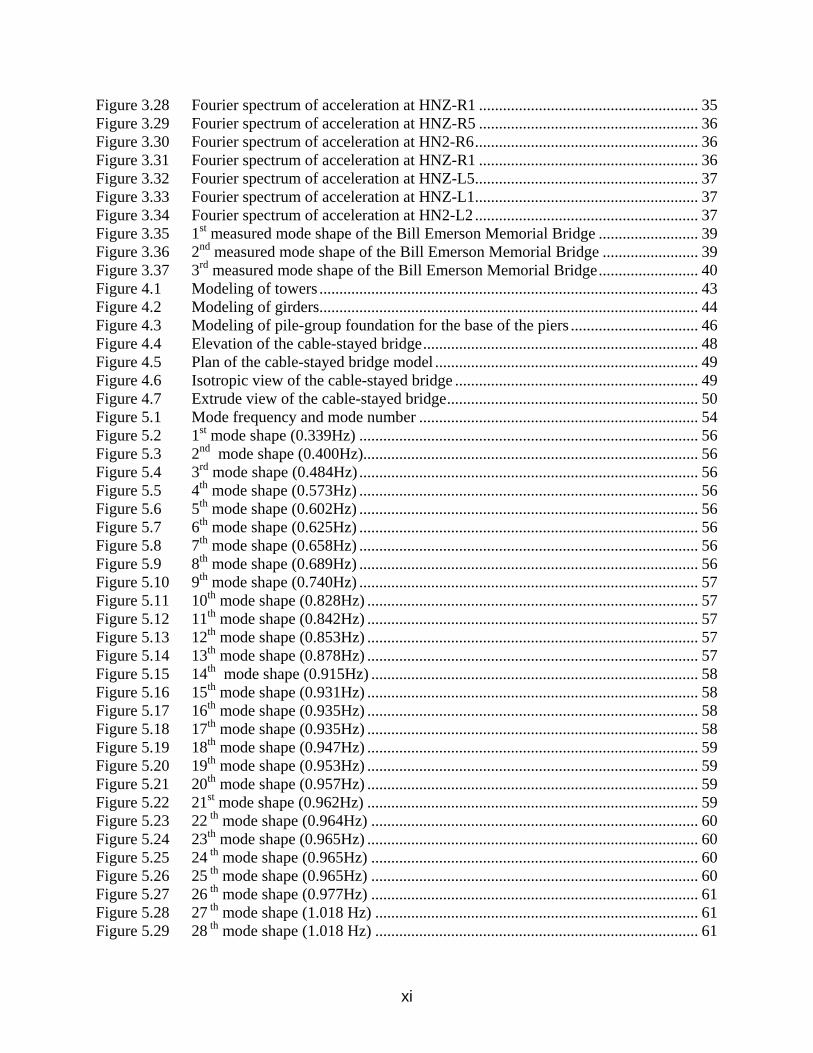
Figure 3.28 Fourier spectrum of acceleration at HNZ-R1 ....................................................... 35 ........................ 36 ........................ 36 ........................ 36 ........................ 37 ........................ 37 ........................ 37 ........................ 39 ........................ 39 ........................ 40 ........................ 43 ........................ 44 ........................ 46 ........................ 48 ........................ 49 ........................ 49 ........................ 50 ........................ 54 ........................ 56 ........................ 56 ........................ 56 ........................ 56 ........................ 56 ........................ 56 ........................ 56 ........................ 56 ........................ 57 ........................ 57 ........................ 57 ........................ 57 ........................ 57 ........................ 58 ........................ 58 ........................ 58 ........................ 58 ........................ 59 ........................ 59 ........................ 59 ........................ 59 ........................ 60 ........................ 60 ........................ 60 ........................ 60 ........................ 61 ........................ 61 ........................ 61

Figure 3.29 Fourier spectrum of acceleration at HNZ-R5 ...............................Figure 3.30 Fourier spectrum of acceleration at HN2-R6................................Figure 3.31 Fourier spectrum of acceleration at HNZ-R1 ...............................Figure 3.32 Fourier spectrum of acceleration at HNZ-L5................................Figure 3.33 Fourier spectrum of acceleration at HNZ-L1................................Figure 3.34 Fourier spectrum of acceleration at HN2-L2................................Figure 3.35 1st measured mode shape of the Bill Emerson Memorial Bridge .Figure 3.36 2nd measured mode shape of the Bill Emerson Memorial BridgeFigure 3.37 3rd measured mode shape of the Bill Emerson Memorial Bridge.Figure 4.1 Modeling of towers .......................................................................Figure 4.2 Modeling of girders.......................................................................Figure 4.3 Modeling of pile-group foundation for the base of the piers ........Figure 4.4 Elevation of the cable-stayed bridge.............................................Figure 4.5 Plan of the cable-stayed bridge model ..........................................Figure 4.6 Isotropic view of the cable-stayed bridge .....................................Figure 4.7 Extrude view of the cable-stayed bridge.......................................Figure 5.1 Mode frequency and mode number ..............................................Figure 5.2 1st mode shape (0.339Hz) .............................................................Figure 5.3 2nd mode shape (0.400Hz)............................................................Figure 5.4 3rd mode shape (0.484Hz) .............................................................Figure 5.5 4th mode shape (0.573Hz) .............................................................Figure 5.6 5th mode shape (0.602Hz) .............................................................Figure 5.7 6th mode shape (0.625Hz) .............................................................Figure 5.8 7th mode shape (0.658Hz) .............................................................Figure 5.9 8th mode shape (0.689Hz) .............................................................Figure 5.10 9th mode shape (0.740Hz) .............................................................Figure 5.11 10th mode shape (0.828Hz) ...........................................................Figure 5.12 11th mode shape (0.842Hz) ...........................................................Figure 5.13 12th mode shape (0.853Hz) ...........................................................Figure 5.14 13th mode shape (0.878Hz) ...........................................................Figure 5.15 14th mode shape (0.915Hz) ..........................................................Figure 5.16 15th mode shape (0.931Hz) ...........................................................Figure 5.17 16th mode shape (0.935Hz) ...........................................................Figure 5.18 17th mode shape (0.935Hz) ...........................................................Figure 5.19 18th mode shape (0.947Hz) ...........................................................Figure 5.20 19th mode shape (0.953Hz) ...........................................................Figure 5.21 20th mode shape (0.957Hz) ...........................................................Figure 5.22 21st mode shape (0.962Hz) ...........................................................Figure 5.23 22 th mode shape (0.964Hz) ..........................................................Figure 5.24 23th mode shape (0.965Hz) ...........................................................Figure 5.25 24 th mode shape (0.965Hz) ..........................................................Figure 5.26 25 th mode shape (0.965Hz) ..........................................................Figure 5.27 26 th mode shape (0.977Hz) ..........................................................Figure 5.28 27 th mode shape (1.018 Hz) .........................................................Figure 5.29 28 th mode shape (1.018 Hz) .........................................................

xi

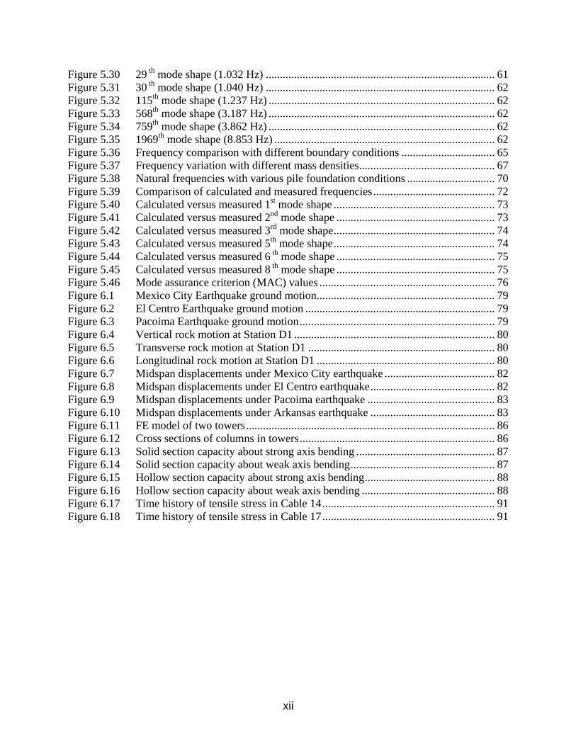
Figure 5.30 29 th mode shape (1.032 Hz) ................................................................................. 61 .............................. 62 .............................. 62 .............................. 62 .............................. 62 .............................. 62 .............................. 65 .............................. 67 .............................. 70 .............................. 72 .............................. 73 .............................. 73 .............................. 74 .............................. 74 .............................. 75 .............................. 75 .............................. 76 .............................. 79 .............................. 79 .............................. 79 .............................. 80 .............................. 80 .............................. 80 .............................. 82 .............................. 82 .............................. 83 .............................. 83 .............................. 86 .............................. 86 .............................. 87 .............................. 87 .............................. 88 .............................. 88 .............................. 91 .............................. 91

Figure 5.31 30 th mode shape (1.040 Hz) ...................................................Figure 5.32 115th mode shape (1.237 Hz) ..................................................Figure 5.33 568th mode shape (3.187 Hz) ..................................................Figure 5.34 759th mode shape (3.862 Hz) ..................................................Figure 5.35 1969th mode shape (8.853 Hz) ................................................Figure 5.36 Frequency comparison with different boundary conditions ...Figure 5.37 Frequency variation with different mass densities..................Figure 5.38 Natural frequencies with various pile foundation conditions .Figure 5.39 Comparison of calculated and measured frequencies.............Figure 5.40 Calculated versus measured 1st mode shape ...........................Figure 5.41 Calculated versus measured 2nd mode shape ..........................Figure 5.42 Calculated versus measured 3rd mode shape...........................Figure 5.43 Calculated versus measured 5th mode shape...........................Figure 5.44 Calculated versus measured 6 th mode shape ..........................Figure 5.45 Calculated versus measured 8 th mode shape ..........................Figure 5.46 Mode assurance criterion (MAC) values ................................Figure 6.1 Mexico City Earthquake ground motion.................................Figure 6.2 El Centro Earthquake ground motion .....................................Figure 6.3 Pacoima Earthquake ground motion.......................................Figure 6.4 Vertical rock motion at Station D1 .........................................Figure 6.5 Transverse rock motion at Station D1 ....................................Figure 6.6 Longitudinal rock motion at Station D1 .................................Figure 6.7 Midspan displacements under Mexico City earthquake .........Figure 6.8 Midspan displacements under El Centro earthquake..............Figure 6.9 Midspan displacements under Pacoima earthquake ...............Figure 6.10 Midspan displacements under Arkansas earthquake ..............Figure 6.11 FE model of two towers..........................................................Figure 6.12 Cross sections of columns in towers.......................................Figure 6.13 Solid section capacity about strong axis bending ...................Figure 6.14 Solid section capacity about weak axis bending.....................Figure 6.15 Hollow section capacity about strong axis bending................Figure 6.16 Hollow section capacity about weak axis bending .................Figure 6.17 Time history of tensile stress in Cable 14...............................Figure 6.18 Time history of tensile stress in Cable 17...............................

xii

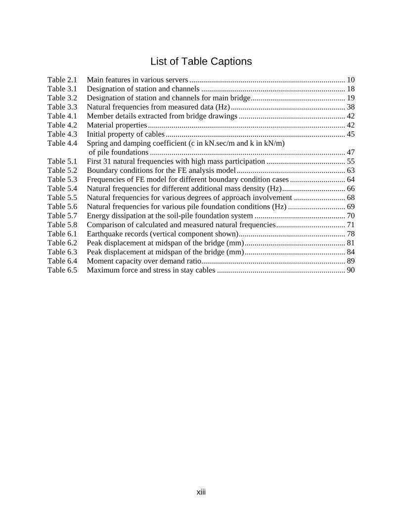
List of Table Captions Table 2.1 Main features in various servers ............................................................................... 10

........................ 18

........................ 19

........................ 38

........................ 42

........................ 42

........................ 45

........................ 47

........................ 55

........................ 63

........................ 64

........................ 66

........................ 68

........................ 69

........................ 70

........................ 71

........................ 78

........................ 81

........................ 84

........................ 89

........................ 90

Table 3.1 Designation of station and channels .................................................Table 3.2 Designation of station and channels for main bridge........................Table 3.3 Natural frequencies from measured data (Hz) ..................................Table 4.1 Member details extracted from bridge drawings ..............................Table 4.2 Material properties ............................................................................Table 4.3 Initial property of cables ...................................................................Table 4.4 Spring and damping coefficient (c in kN.sec/m and k in kN/m)

of pile foundations ...........................................................................Table 5.1 First 31 natural frequencies with high mass participation ................Table 5.2 Boundary conditions for the FE analysis model ...............................Table 5.3 Frequencies of FE model for different boundary condition cases ....Table 5.4 Natural frequencies for different additional mass density (Hz)........Table 5.5 Natural frequencies for various degrees of approach involvement ..Table 5.6 Natural frequencies for various pile foundation conditions (Hz) .....Table 5.7 Energy dissipation at the soil-pile foundation system ......................Table 5.8 Comparison of calculated and measured natural frequencies...........Table 6.1 Earthquake records (vertical component shown)..............................Table 6.2 Peak displacement at midspan of the bridge (mm)...........................Table 6.3 Peak displacement at midspan of the bridge (mm)...........................Table 6.4 Moment capacity over demand ratio.................................................Table 6.5 Maximum force and stress in stay cables .........................................

xiii

1. Introduction 1.1. General

Cable-stayed bridge is an elegant, economical and efficient structure and now it is becoming more and more popular throughout the world. In the past several decades, the United States has witnessed a rapid development in the construction of this type of bridges. Due to its good characteristics in earthquake resistance, it has even become the first choice of the construction of a bridge in seismic zones with high risks (Hu et al., 2006). With the rapid progress in analysis tools and construction technologies, the main span of cable-stayed bridges has been pushed much longer in recent years. For example, the length of the main span is 605 m (1985 ft), 886 m (2907 ft), and 890 m (2907 ft) for Qingzhou Bridge (Ming River, China), Pont de Bridge (Normandie, France), and Tartara Bridge (Hiroshima, Japan), respectively. With ever increasing span lengths, cable-stayed bridges behave in a more complicated way, and often become more susceptible to environmental effects. The fundamental characteristics such as stiffness of structural members, variation of cable forces, and stability of structural systems play a more critical role in the safety evaluation of these bridges.

Although a cable-stayed bridge seems subjected to high stresses under gravity loads, it is generally sensitive to dynamic loadings resulting from earthquakes, winds and moving vehicles. In these cases, the condition of a large span cable-stayed bridge must be assessed to ensure the smooth operation and safety during its life span. One way to assess a structure is to observe changes in vibration characteristics such as natural frequencies, damping ratios and mode shapes of bridges. Those changes, if properly identified and classified, can provide a viable means for damage detection of the structure (Roebling et al., 1996; Ren et al., 2005; Wang et al., 2007). The other way of structural assessment is to conduct extensive dynamic analyses in frequency domain (Allam and Datta, 1999) to understand the behavior of the structure by comparing load/displacement with strength/ductility.

Field tests provide an effective way of characterizing a cable-stayed bridge structure for its mechanic and dynamic properties (Hu et al., 2006). They can be performed under three types of loadings: harmonic excitation, initial disturbance, and ambient excitation. In harmonic/force vibration tests, bridges are excited by a shaker or other artificial means. In this case, both input and output can be obtained. By using a known forcing function, many of the uncertainties associated with data collection and processing can be avoided. For large-scale bridge structures, however, generating significant vibration requires the use of a heavy shaker or other equipment, which often makes this method impractical. Free vibration tests are carried out by suddenly releasing a heavy load or mass appropriately connected to the bridge. The induced free vibration decays and energy dissipates as a result of friction or heat generation. The free vibration records can be analyzed to determine the properties of the bridge structure. Both forced vibration and free vibration are excited by the use of an artificial means with no traffic on the bridge during tests. This requirement often causes great inconvenience for existing bridges. As a result, ambient vibration tests are preferred in many applications. They take advantage of the vibration sources available during regular operations, including wind and earthquake

1

effects, vehicle impact, wave effects, or ground motion generated by adjacent industries or due to construction. They correspond to an actual operating condition of bridges and will thus not interrupt any traffic or service of the bridges.

Due to its structural complexity, a long span cable-stayed bridge is often modeled with finite elements of various components to evaluate the dynamic characteristics and responses of the bridge structure (John et al., 2005). For example, Wilson et al. (1991) established a three-dimensional finite element model of a cable-stayed bridge structure, including the bridge deck, towers, cables, and bearings. The finite element (FE) model took into account the translational and rotational mass and stiffness of the bridge deck, and included an accurate geometric representation of bearings. Its modal properties were validated with those of the ambient vibration measured from the bridge. With established FE models, Ren (1999) and Ren and Obata (1999) investigated the elastic-plastic seismic behavior, nonlinear static behavior, and ultimate behavior of long span cable-stayed bridges over the Ming River. Ren et al. (2005, 2007) also studied the behavior of the Qingzhou cable-stayed bridge both numerically and experimentally. Modeling issues such as initial equilibrium configuration, geometrical nonlinearity, concrete slab stiffness in the composite deck, shear connection between concrete slab and steel girders, and longitudinal restraints of side expansion joints were discussed. These studies enrich the current knowledge in understanding the dynamic behavior of large-span cable-stayed bridges.

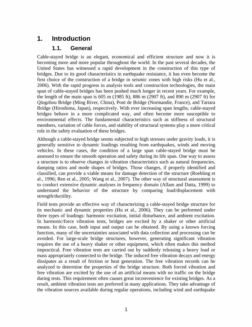
1.2. Bridge description The Bill Emerson Memorial Bridge is a 1206 m (3956 ft) long, cable-stayed structure carrying Missouri State Highway 34, Missouri State Highway 74 and Illinois Route 146 across the Mississippi River between Cape Girardeau, Missouri, and East Cape Girardeau, Illinois. Its coordinates are 37°17′43″N and 89°30′57″W. The bridge was opened to traffic on December 13, 2003. As schematically shown in Figures 1.1, 1.2 and 1.3, the final design of the bridge includes two towers, 128 cables, and 12 additional piers in the approach span on the Illinois side. The typical cross section of deck is shown in Figure 1.4.

2

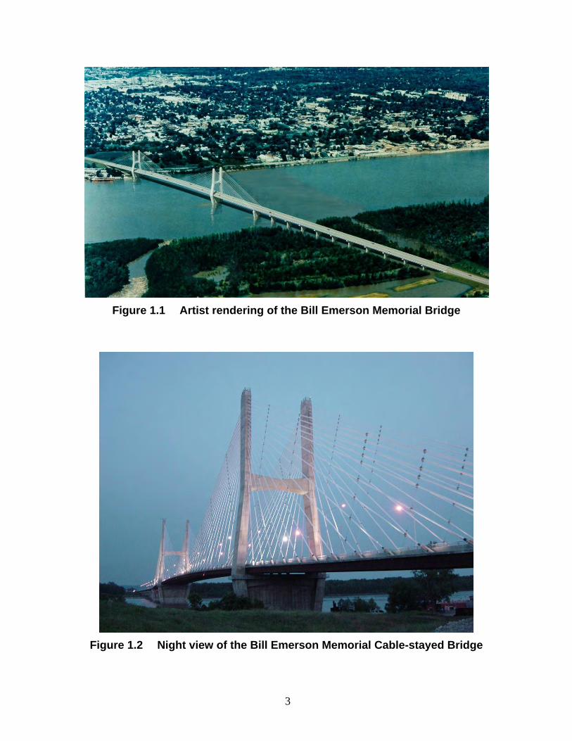
Figure 1.1 Artist rendering of the Bill Emerson Memorial Bridge

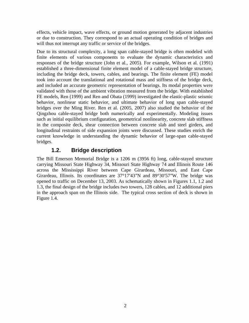
Figure 1.2 Night view of the Bill Emerson Memorial Cable-stayed Bridge

3

142.7 m 350.6 m 142.7 m 570 m

Illinois approach

End Pier 2 Pier 4 Bent 1 Pier 3

Figure 1.3 Schematic view of the Bill Emersion Memorial Cable-stayed Bridge

0.67 m 14.0 m 14.0 m 0.67 m

Concrete slab Barrier Steel girder Floor beam

Figure 1.4 Typical cross section of the bridge deck

The bridge has a total length of 1206 m (3956 ft). It consists of one 350.6 m (1150 ft) long main span, two 142.7 m (468 ft) long side spans, and one 570 m (1870 ft) long approach span on the Illinois side. The main span of the bridge provides more than 18.3 m (60 ft) of vertical clearance over the navigation channel. The 12 piers on the approach span have 11 equal spacings of 51.8 m (170 ft) each. Carrying two-way traffic, the bridge has four 3.66 m (12 ft) wide vehicular lanes plus two narrower shoulders. The total width of the bridge deck is 29.3 m (96 ft) as shown in Figure 1.4. The deck is composed of two longitudinal built-up steel girders, a longitudinal center strut, transverse floor beams, and precast concrete slabs. A concrete barrier is located in the center of the bridge, and two railings and additional concrete barriers are located along the edges of the deck. Pier 2 rests on rock while Pier 3 and Pier 4 foundations are supported on two separate caissons.

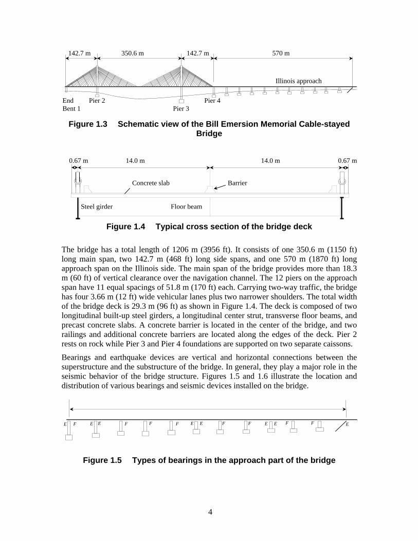
Bearings and earthquake devices are vertical and horizontal connections between the superstructure and the substructure of the bridge. In general, they play a major role in the seismic behavior of the bridge structure. Figures 1.5 and 1.6 illustrate the location and distribution of various bearings and seismic devices installed on the bridge.

E F E E F F F F E E EF F EF E

Figure 1.5 Types of bearings in the approach part of the bridge

4

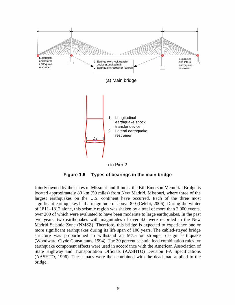
1. Earthquake shock transfer device (Longitudinal)

2. Earthquake restrainer (lateral)

Expansion and lateral earthquake restrainer

Expansion and lateral earthquake restrainer

(a) Main bridge

1. Longitudinal earthquake shock transfer device

2. Lateral earthquake restrainer

21 12

(b) Pier 2

Figure 1.6 Types of bearings in the main bridge

Jointly owned by the states of Missouri and Illinois, the Bill Emerson Memorial Bridge is located approximately 80 km (50 miles) from New Madrid, Missouri, where three of the largest earthquakes on the U.S. continent have occurred. Each of the three most significant earthquakes had a magnitude of above 8.0 (Celebi, 2006). During the winter of 1811–1812 alone, this seismic region was shaken by a total of more than 2,000 events, over 200 of which were evaluated to have been moderate to large earthquakes. In the past two years, two earthquakes with magnitudes of over 4.0 were recorded in the New Madrid Seismic Zone (NMSZ). Therefore, this bridge is expected to experience one or more significant earthquakes during its life span of 100 years. The cabled-stayed bridge structure was proportioned to withstand an M7.5 or stronger design earthquake (Woodward-Clyde Consultants, 1994). The 30 percent seismic load combination rules for earthquake component effects were used in accordance with the American Association of State Highway and Transportation Officials (AASHTO) Division I-A Specifications (AASHTO, 1996). These loads were then combined with the dead load applied to the bridge.

5

1.3. Seismic instrumentation system In seismically active regions such as the NMSZ, acquisition of structural response and nearby free field response data during earthquakes or other extreme loading events, e.g., blasts, is essential to evaluate current design practices and develop new methodologies for future analysis, design, and retrofitting of infrastructure systems. Due to its criticality and proximity to the NMSZ as well as lack of significant measured ground motions, the Bill Emerson Memorial Cable-stayed Bridge and its adjacent area were installed with an 84-channel seismic instrumentation system. The so-called ASPEN system was processed and developed by a group comprised of the Federal Highway Administration (FHWA), Missouri Department of Transportation (MoDOT), HNTB Corp., Multidisciplinary Center for Earthquake Engineering Research (MCEER), and United States Geological Survey (USGS). The system consists of a total of 84 Kinemetrics EpiSensor accelerometers, Q330 digitizers, and Baler units for data concentrator and mass storage. These hardware components were designed and installed on the bridge by Kinemetrics Inc. Antennas were installed on two bridge towers at Pier 2 and Pier 3, at free field sites on the Illinois end of the bridge, and on the central recording building near the bridge, so wireless communication of data can be initiated among various locations as well as from the bridge and free field sites to the off-structure central recording building.

The accelerometers installed throughout the bridge structure and adjacent free field sites allow the recording of structural vibrations of the bridge and free field motions at the surface and down-hole locations. They were deployed such that the acquired data can be used to understand the overall response and behavior of the cable-stayed bridge, including translational, torsional, rocking, and translational soil-structure interactions at foundation levels. The acquired data also can be used by the researchers and designers to check seismic design parameters and to compare dynamic characteristics with those from actual dynamic responses. The comprehensive understanding of the long-span, cable-stayed bridge will benefit other similar bridge seismic design, especially for those also located in the same seismic zone.

1.4. Scope of work The primary goal of this investigation is to evaluate the structural dynamic characteristics of the Bill Emerson Memorial Cable-stayed Bridge. The objectives of the study are to retrieve peak ground motions at the bridge site and to verify the assumptions made in the structural design of the bridge. The approach taken to verify the design assumptions is to develop a well-calibrated FE model of the cable-stayed bridge, and to study the behavior and load path of the bridge structure. To achieve the objectives above, the scope of work includes:

1. Develop a methodology and necessary tools for automatic compiling of the peak ground and structural accelerations.

2. Establish a 3-D FE model of the bridge including multi-support excitations and soil-structure interaction so that realistic behaviors of the bridge can be simulated numerically. Both the main and approach spans will be modeled with a commercial program (SAP2000) that is suitable for modeling of superstructure, substructure, and pile foundations.

6

3. Evaluate the model by conducting sensitivity analysis, checking boundary conditions and compatibility of various parts of the bridge, and making necessary engineering judgments. Sensitivity analysis will ensure that the modeling of various parts of the bridge is consistent in terms of member types, geometrical and material properties. Connectivity among various structural members at a joint could be pretty complicated in a cable-stayed bridge. It needs to be properly modeled.

4. Determine the bridge’s dynamic characteristics such as vibration mode shapes and frequencies. The dynamic characteristics of the bridge will be identified from the measured accelerations due to ambient vibration and they will be compared with the calculated values from the FE model.

5. Verify the assumptions used in the design of the bridge structure by understanding the structural behavior and load path with the well-calibrated FE model when both ground motions and structural responses at critical locations are known.

1.5. Significant of this study A number of long-span bridges exist near the New Madrid Seismic Zone (NMSZ). Many of these bridges are subjected to direct threats from the NMSZ where the largest continental earthquake in the US history occurred in 1811-1812. Service outage of these bridges due to earthquake-induced failure will not only cause traffic congestion in region but also sever the nation’s ground transportation link along the corridor from California to New York. The public perception to any of these potential incidences is significant.

This study helps understand the seismic behavior of the Bill Emerson Memorial Cable-stayed Bridge under a design earthquake. It identifies key areas and structural components for inspection of the bridge after a strong earthquake event in the future.

The cable-stayed bridge system is unique in several ways, including the combined rock and soil conditions, the new design feature of towers. This study validates some of the design assumptions by assessing the integrity of the cable-stayed bridge under a postulated design earthquake based on the acceleration records during a minor earthquake.

This study provides a baseline three-dimensional model of the cable-stayed bridge that has been validated with field measurements. This model can further be used to develop damage detection and health monitoring schemes of the bridge to arrive at the so called condition-based inspection of bridge conditions or provide a critical supplement to visual inspection in current practices. The model can also be used to develop and validate control technologies such as those studied by Agrawal et al. (2003) and Dyke et al. (2003).

1.6. Organization of this report This report is divided into seven major sections. Section 1 gives a general introduction on the Bill Emerson Memorial Cable-stayed Bridge, the seismic instrumentation system, scope and significance of this study. Section 2 presents a process and methodology to retrieve the peak accelerations in a fixed time window from the continuous data collected in real time. In Section 3, some of the collected data from the instrumentation system are

7

processed and analyzed for FE model validation in Section 5. Section 4 discusses the FE modeling of the cable-stayed bridge and Section 5 investigates the sensitivity of the FE model to pertinent parameters and conditions and validates the model with measured data. In Section 6, the validated FE model is applied to determine the seismic demand on various structural components under a design earthquake for the assessment of the cable-stayed bridge. Section 7 summarizes the conclusions and recommendations derived from this study.

8

2. Automatic Retrieval of Peak Accelerations from Real-time Seismic Instrumentation System

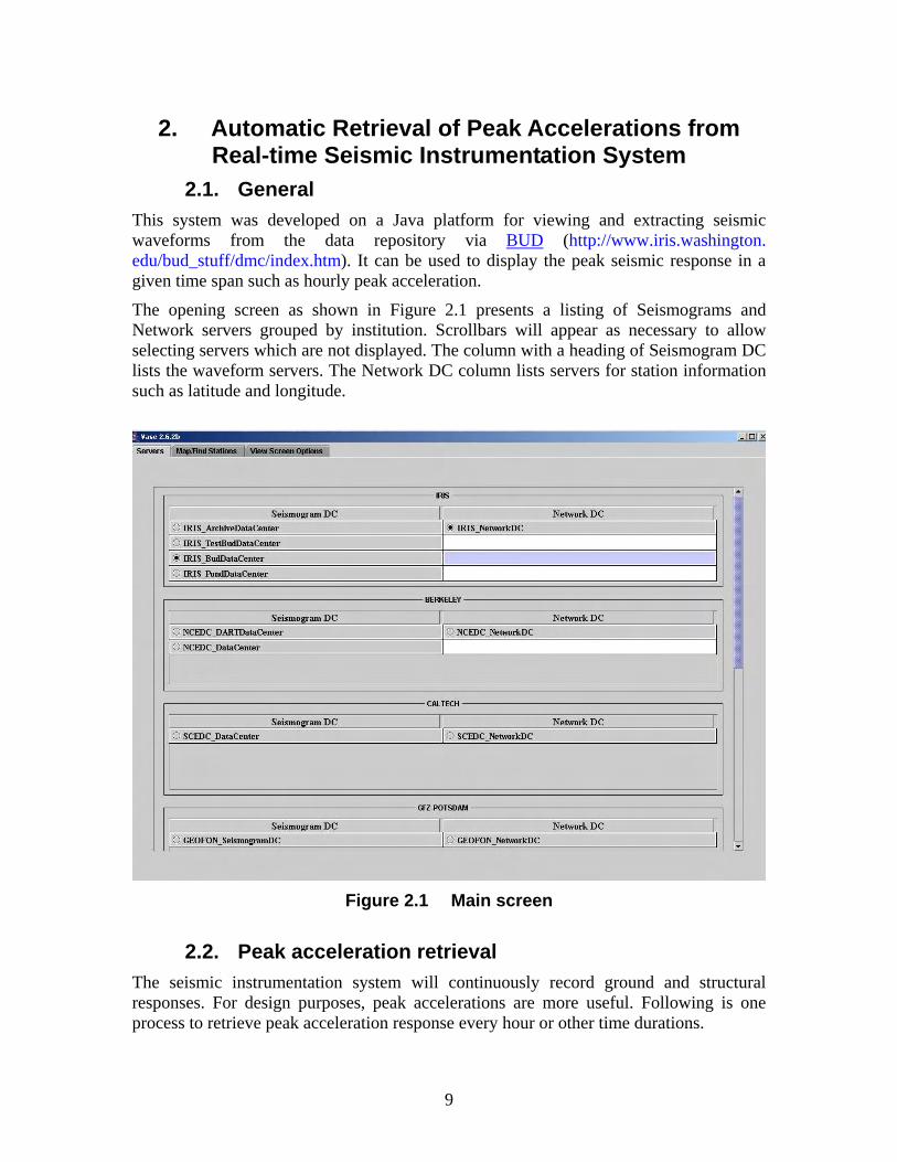
2.1. General This system was developed on a Java platform for viewing and extracting seismic waveforms from the data repository via BUD (http://www.iris.washington. edu/bud_stuff/dmc/index.htm). It can be used to display the peak seismic response in a given time span such as hourly peak acceleration.

The opening screen as shown in Figure 2.1 presents a listing of Seismograms and Network servers grouped by institution. Scrollbars will appear as necessary to allow selecting servers which are not displayed. The column with a heading of Seismogram DC lists the waveform servers. The Network DC column lists servers for station information such as latitude and longitude.

Figure 2.1 Main screen

2.2. Peak acceleration retrieval The seismic instrumentation system will continuously record ground and structural responses. For design purposes, peak accelerations are more useful. Following is one process to retrieve peak acceleration response every hour or other time durations.

9

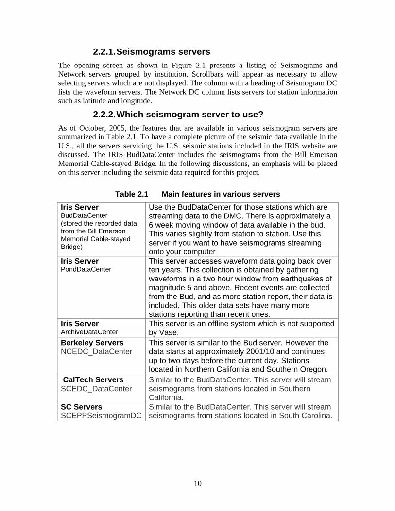
2.2.1. Seismograms servers The opening screen as shown in Figure 2.1 presents a listing of Seismograms and Network servers grouped by institution. Scrollbars will appear as necessary to allow selecting servers which are not displayed. The column with a heading of Seismogram DC lists the waveform servers. The Network DC column lists servers for station information such as latitude and longitude.

2.2.2. Which seismogram server to use? As of October, 2005, the features that are available in various seismogram servers are summarized in Table 2.1. To have a complete picture of the seismic data available in the U.S., all the servers servicing the U.S. seismic stations included in the IRIS website are discussed. The IRIS BudDataCenter includes the seismograms from the Bill Emerson Memorial Cable-stayed Bridge. In the following discussions, an emphasis will be placed on this server including the seismic data required for this project.

Table 2.1 Main features in various servers

Iris Server BudDataCenter (stored the recorded data from the Bill Emerson Memorial Cable-stayed Bridge)

Use the BudDataCenter for those stations which are streaming data to the DMC. There is approximately a 6 week moving window of data available in the bud. This varies slightly from station to station. Use this server if you want to have seismograms streaming onto your computer

Iris Server This server accesses waveform data going back over PondDataCenter ten years. This collection is obtained by gathering

waveforms in a two hour window from earthquakes of magnitude 5 and above. Recent events are collected from the Bud, and as more station report, their data is included. This older data sets have many more stations reporting than recent ones.

Iris Server ArchiveDataCenter

This server is an offline system which is not supported by Vase.

Berkeley Servers NCEDC_DataCenter

This server is similar to the Bud server. However the data starts at approximately 2001/10 and continues up to two days before the current day. Stations located in Northern California and Southern Oregon.

CalTech Servers Similar to the BudDataCenter. This server will stream SCEDC_DataCenter seismograms from stations located in Southern

California. SC Servers Similar to the BudDataCenter. This server will stream SCEPPSeismogramDC seismograms from stations located in South Carolina.

10

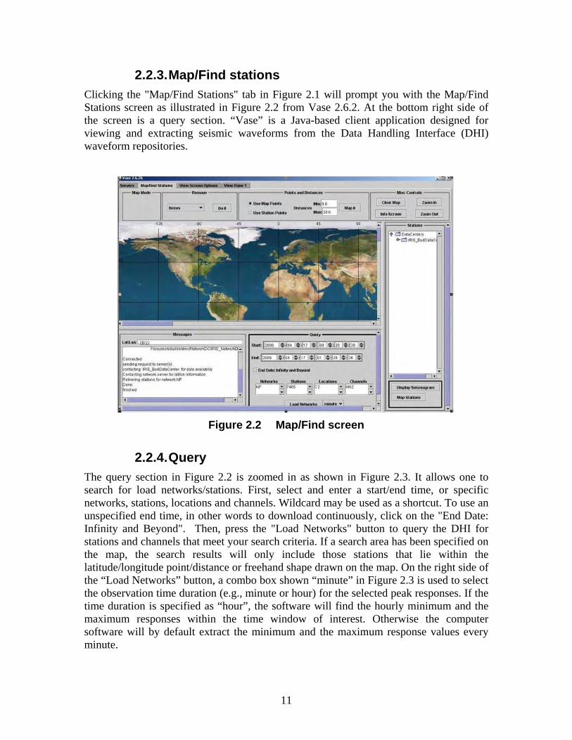
2.2.3. Map/Find stations Clicking the "Map/Find Stations" tab in Figure 2.1 will prompt you with the Map/Find Stations screen as illustrated in Figure 2.2 from Vase 2.6.2. At the bottom right side of the screen is a query section. “Vase” is a Java-based client application designed for viewing and extracting seismic waveforms from the Data Handling Interface (DHI) waveform repositories.

Figure 2.2 Map/Find screen

2.2.4. Query The query section in Figure 2.2 is zoomed in as shown in Figure 2.3. It allows one to search for load networks/stations. First, select and enter a start/end time, or specific networks, stations, locations and channels. Wildcard may be used as a shortcut. To use an unspecified end time, in other words to download continuously, click on the "End Date: Infinity and Beyond". Then, press the "Load Networks" button to query the DHI for stations and channels that meet your search criteria. If a search area has been specified on the map, the search results will only include those stations that lie within the latitude/longitude point/distance or freehand shape drawn on the map. On the right side of the “Load Networks” button, a combo box shown “minute” in Figure 2.3 is used to select the observation time duration (e.g., minute or hour) for the selected peak responses. If the time duration is specified as “hour”, the software will find the hourly minimum and the maximum responses within the time window of interest. Otherwise the computer software will by default extract the minimum and the maximum response values every minute.

11

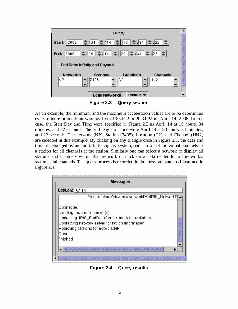
Figure 2.3 Query section

As an example, the minimum and the maximum acceleration values are to be determined every minute in one hour window from 19:34:22 to 20:34:22 on April 14, 2006. In this case, the Start Day and Time were specified in Figure 2.2 as April 14 at 19 hours, 34 minutes, and 22 seconds. The End Day and Time were April 14 at 20 hours, 34 minutes, and 22 seconds. The network (NP), Station (7405), Location (C2), and Channel (HN2) are selected in this example. By clicking on any triangle once in Figure 2.3, the data and time are changed by one unit. In this query system, one can select individual channels or a station for all channels at the station. Similarly one can select a network to display all stations and channels within that network or click on a data center for all networks, stations and channels. The query process is recorded in the message panel as illustrated in Figure 2.4.

Figure 2.4 Query results

12

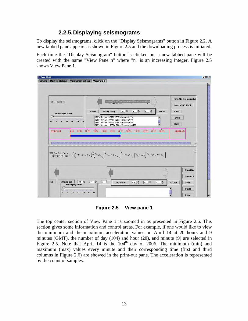
2.2.5. Displaying seismograms To display the seismograms, click on the "Display Seismograms" button in Figure 2.2. A new tabbed pane appears as shown in Figure 2.5 and the downloading process is initiated.

Each time the "Display Seismogram" button is clicked on, a new tabbed pane will be created with the name "View Pane n" where "n" is an increasing integer. Figure 2.5 shows View Pane 1.

Figure 2.5 View pane 1 The top center section of View Pane 1 is zoomed in as presented in Figure 2.6. This section gives some information and control areas. For example, if one would like to view the minimum and the maximum acceleration values on April 14 at 20 hours and 9 minutes (GMT), the number of day (104) and hour (20), and minute (9) are selected in Figure 2.5. Note that April 14 is the 104th day of 2006. The minimum (min) and maximum (max) values every minute and their corresponding time (first and third columns in Figure 2.6) are showed in the print-out pane. The acceleration is represented by the count of samples.

13

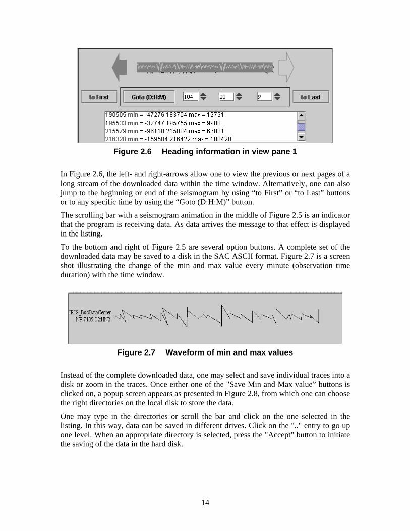
Figure 2.6 Heading information in view pane 1

In Figure 2.6, the left- and right-arrows allow one to view the previous or next pages of a long stream of the downloaded data within the time window. Alternatively, one can also jump to the beginning or end of the seismogram by using “to First” or “to Last” buttons or to any specific time by using the “Goto (D:H:M)” button.

The scrolling bar with a seismogram animation in the middle of Figure 2.5 is an indicator that the program is receiving data. As data arrives the message to that effect is displayed in the listing.

To the bottom and right of Figure 2.5 are several option buttons. A complete set of the downloaded data may be saved to a disk in the SAC ASCII format. Figure 2.7 is a screen shot illustrating the change of the min and max value every minute (observation time duration) with the time window.

Figure 2.7 Waveform of min and max values

Instead of the complete downloaded data, one may select and save individual traces into a disk or zoom in the traces. Once either one of the "Save Min and Max value” buttons is clicked on, a popup screen appears as presented in Figure 2.8, from which one can choose the right directories on the local disk to store the data.

One may type in the directories or scroll the bar and click on the one selected in the listing. In this way, data can be saved in different drives. Click on the ".." entry to go up one level. When an appropriate directory is selected, press the "Accept" button to initiate the saving of the data in the hard disk.

14

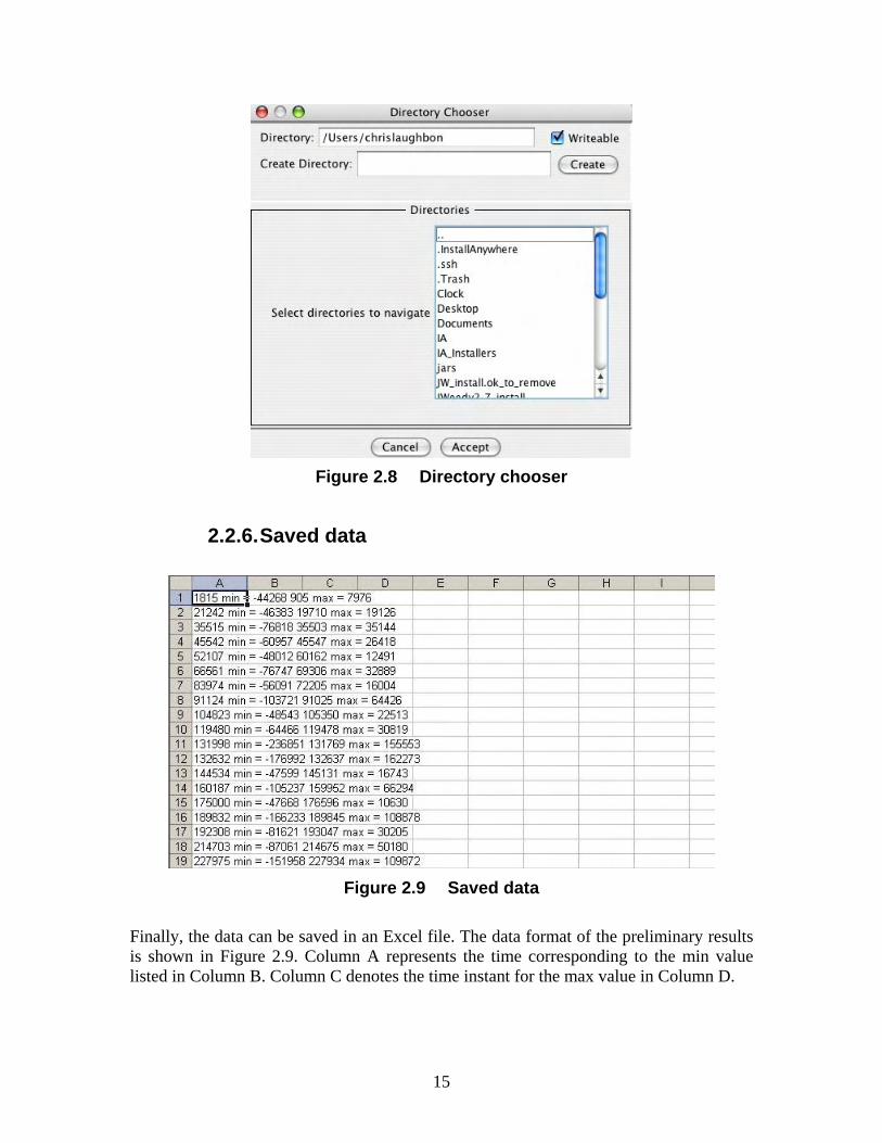
Figure 2.8 Directory chooser

2.2.6. Saved data

Figure 2.9 Saved data

Finally, the data can be saved in an Excel file. The data format of the preliminary results is shown in Figure 2.9. Column A represents the time corresponding to the min value listed in Column B. Column C denotes the time instant for the max value in Column D.

15

3. Seismic Instrumentation System and Measured Data Analysis

3.1. General Field test generally provides an effective means to investigate the fundamental behavior of cable-stayed bridges (Hu et al., 2006). Three types of field tests have been widely used in determining the mechanical properties of long span cable-stayed bridges (Okauchi et al., 1997; Ren et al., 2005; Cunha et al., 2006; Hsieh et al., 2006; Hu et al., 2006):

♦

♦

♦

Forced vibration tests;

Free vibration tests;

Ambient vibration tests.

In forced vibration tests, bridges are usually excited by artificial means and thus both input and output data can be obtained. Input parameters for these tests include the type, amplitude, frequency content, duration, and time of decay of waveforms as well as the location of excitation loads. With a known forcing function, many of the uncertainties associated with data collection and processing can be avoided. Additionally, although at any given time a structural response results from all sources of excitations, filtering techniques can be used to separate their effects and determine part of the response to a specific source. The amplitude of forced vibration can also be designed to be significantly higher than the ambient or electronic noise levels in order to increase the signal-to-noise ratio and more accurately evaluate the properties of a bridge structure. For large-scale civil engineering structures, however, this technique is often impractical since it requires heavy and expensive equipment to generate a controlled and significant excitation.

Free vibration tests are carried out by a sudden release of a heavy load or mass appropriately connected to a bridge. Over time, the potential energy originally stored in the bridge structure gradually dissipates due to friction or heat generation, resulting in the free vibration decay. The free vibration data can be analyzed to determine the properties of the structure. In the free vibration tests by Cunha et al. (2001), a suspended mass was suddenly released from the deck of the Vasco da Gama Cable-stayed Bridge. In both forced and free vibration tests, bridges need to be excited by an artificial means. In most cases, traffic must be interrupted during tests, which causes inconvenience to travelers.

Ambient vibration tests take advantage of natural sources of bridge vibration. They require no equipment to excite the bridge to be tested. Ambient vibration is induced by wind, minor earthquake, traffic, wave, and ground motion generated by nearby construction or industrial activities. It corresponds to the real operation condition of bridges and thus requires no traffic interruption during tests (Abdel-Ghaffer and Scanlan, 1985; Brownjohn et al., 1989; Brownjohn et al., 1999; Wilson et al., 1991; Xu et al., 1997; Macdonald and Wendy, 2005). In this study, field measured data from traffic and minor earthquake are analyzed to understand the dynamics and properties of the Bill Emerson Memorial Cable-stayed Bridge.

16

3.2. Seismic instrumentation network The Bill Emerson Memorial Cable-stayed Bridge was instrumented with a real-time seismic monitoring system named ASPEN. Accelerometers were installed inside downholes at two nearby free fields and various parts of the bridge, including deck, towers, and foundations. In earthquake engineering, instrumentation can be grouped into three main categories (Celebi, 2006). The first category is bridge instrumentation of the superstructure and substructure to capture and define (a) the overall motion of the cable-stayed bridge, (b) the motion of the two towers to assess their translational and torsional behavior relative to the caissons and deck levels, (c) the deck motion to assess the dynamic behavior of the deck including fundamental and higher modes in three directions, and (d) at bents of the bridge, intermediate pier locations, and bottom of foundations to understand the ground motions and interaction between foundation and the superstructure. The second category is instrumentation of the free fields in the vicinity of the bridge including those downhole measurements to assess the different ground motions near the bridge. The third category is instrumentation array for ground failures near the bridge. The Bill Emerson Memorial Bridge instrumentation fell into the first and second categories.

Data recorded from the Bill Emerson Memorial Bridge have been transmitted to and stored in the Data Management Center of the Incorporated Research Institutions for Seismology system (IRIS: http://www.iris.edu). These data are stored under the station of “NP” of the Center Recording System of the Bill Emerson Memorial Cable-stayed Bridge Seismic Monitoring System. The data transmitted to IRIS is in mini-seed format, and all streamed data from the bridge will be stored and available for four to eight weeks. After that, the stored data will be deleted except for significant earthquake data. More information about the seismic monitoring system can be found in Celebi (2004).

A total of 43 stations and 84 channels of acceleration records are listed in Table 3.1. In Table 3.1, HN2 represents the transverse/lateral component perpendicular to the traffic direction, HN3 means the traffic direction of the bridge or longitudinal component, and HNZ is the vertical component. The stations and channels are distributed on the bridge as illustrated in Figure 3.1. Each arrow in Figure 3.1 indicates one channel of acceleration data. The seismic instrumentation system on the Bill Emerson Memorial Cable-stayed Bridge continuously provides the structural vibration and soil responses at free field sites. As such, the bridge can be used for real-time monitoring of structural conditions. The real-time monitoring system has been reliably collecting data since February to March 2004.

17

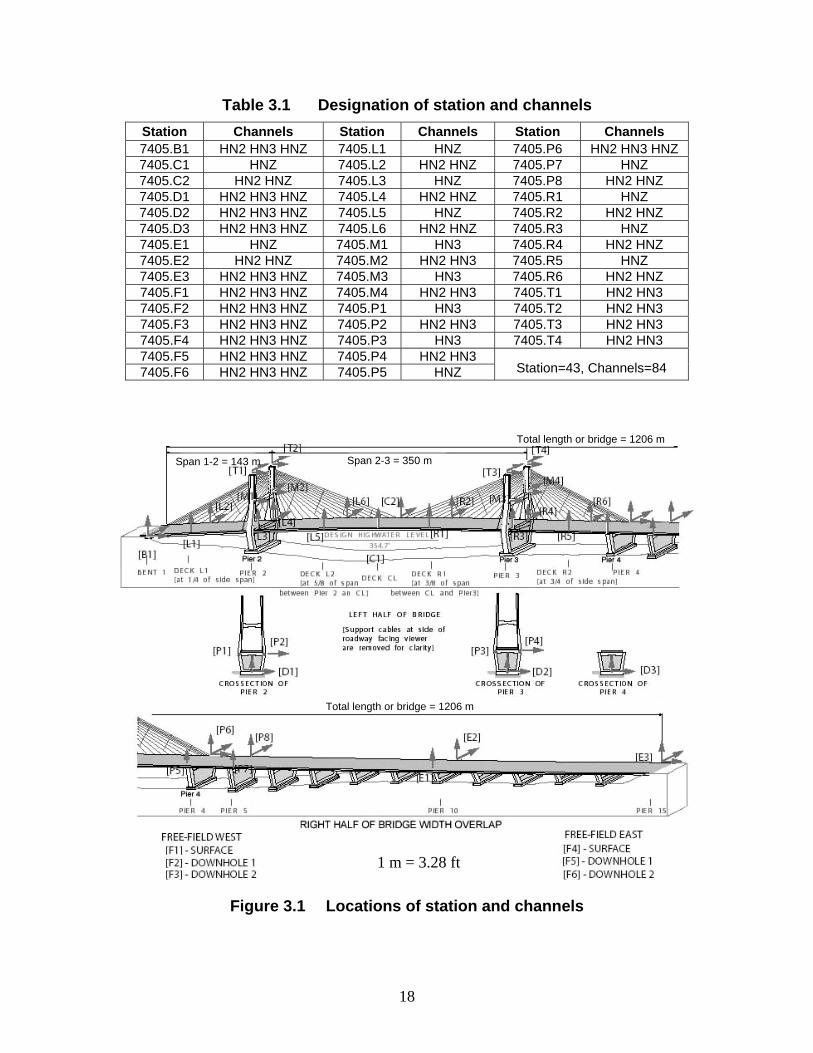
Table 3.1 Designation of station and channels Station Channels Station Channels Station Channels 7405.B1 HN2 HN3 HNZ 7405.L1 HNZ 7405.P6 HN2 HN3 HNZ 7405.C1 HNZ 7405.L2 HN2 HNZ 7405.P7 HNZ 7405.C2 HN2 HNZ 7405.L3 HNZ 7405.P8 HN2 HNZ 7405.D1 HN2 HN3 HNZ 7405.L4 HN2 HNZ 7405.R1 HNZ 7405.D2 HN2 HN3 HNZ 7405.L5 HNZ 7405.R2 HN2 HNZ 7405.D3 HN2 HN3 HNZ 7405.L6 HN2 HNZ 7405.R3 HNZ 7405.E1 HNZ 7405.M1 HN3 7405.R4 HN2 HNZ7405.E2 HN2 HNZ 7405.M2 HN2 HN3 7405.R5 HNZ 7405.E3 HN2 HN3 HNZ 7405.M3 HN3 7405.R6 HN2 HNZ 7405.F1 HN2 HN3 HNZ 7405.M4 HN2 HN3 7405.T1 HN2 HN3 7405.F2 HN2 HN3 HNZ 7405.P1 HN3 7405.T2 HN2 HN3 7405.F3 HN2 HN3 HNZ 7405.P2 HN2 HN3 7405.T3 HN2 HN3 7405.F4 HN2 HN3 HNZ 7405.P3 HN3 7405.T4 HN2 HN3 7405.F5 HN2 HN3 HNZ 7405.P4 HN2 HN3

Station=43, Channels=84 7405.F6 HN2 HN3 HNZ 7405.P5 HNZ

Total length or bridge = 1206 m

Span 2-3 = 350 m Span 1-2 = 143 m

Total length or bridge = 1206 m

1 m = 3.28 ft

Figure 3.1 Locations of station and channels

18

The main bridge from Bent 1 to Pier 4 includes one main span and two side spans of the cable-stayed structure. It is separated from the Illinois approach by an expansion joint on top of Pier 4. At the expansion joints, the main bridge and the Illinois approach have the same displacement in the transverse direction but independent longitudinal moment, resulting in a relatively weak connection between two parts. Those channels in Table 3.1, which are located on the main bridge, are re-listed in Table 3.2. A total of 32 stations and 67 channels are on the main bridge. Among the 32 stations, D1, D2 and D3 are located at the top of the foundation. The records at these stations approximately represent the rock motion of the bridge during earthquakes.

Table 3.2 Designation of station and channels for main bridge

Station Channels Station Channels Station Channels 7405.B1 HN2 HN3 HNZ 7405.L6 HN2 HNZ 7405.R1 HNZ 7405.C1 HNZ 7405.M1 HN3 7405.R2 HN2 HNZ 7405.C2 HN2 HNZ 7405.M2 HN2 HN3 7405.R3 HNZ 7405.D1 HN2 HN3 HNZ 7405.M3 HN3 7405.R4 HN2 HNZ 7405.D2 HN2 HN3 HNZ 7405.M4 HN2 HN3 7405.R5 HNZ 7405.D3 HN2 HN3 HNZ 7405.P1 HN3 7405.R6 HN2 HNZ 7405.L1 HNZ 7405.P2 HN2 HN3 7405.T1 HN2 HN3 7405.L2 HN2 HNZ 7405.P3 HN3 7405.T2 HN2 HN3 7405.L3 HNZ 7405.P4 HN2 HN3 7405.T3 HN2 HN3 7405.L4 HN2 HNZ 7405.P5 HNZ 7405.T4 HN2 HN3 7405.L5 HNZ 7405.P6 HN2 HN3 HNZ Station=32; Channels= 67

3.3. Measured data The dynamic responses of the bridge induced by earthquake excitations and traffic loads can be obtained from the seismic instrumentation system. In this section, some response data from the system are analyzed. Two sets of field-measured data were selected. One set is two minutes of traffic-induced vibration data in a time period from 19:20′40″ to 19:22′40″ on July 25, 2006. Although a Richter’s Magnitude 2.2 earthquake occurred at 19:35′39″ (Universal Time) on July 25, 2006, in southeastern Missouri (36.76N and 89.49W), the response at the bridge site was negligible. The other set of data was induced by an earthquake event, which occurred at 12:37′32″ on May 1, 2005 with a Richter's Magnitude 4.1. The epicenter of the earthquake was located at four miles SSE (162o) from Manila, Arkansas and 180 km (111 miles) from the bridge. The hypocentral depth was estimated to be 10 km (6.2 miles). This section presents an analysis of the vertical, transverse, and longitudinal acceleration responses at the bridge deck and towers. In the following section, some of the corresponding amplitude spectra at various deck and tower locations will be presented to compare with the frequencies obtained from numerical simulations.

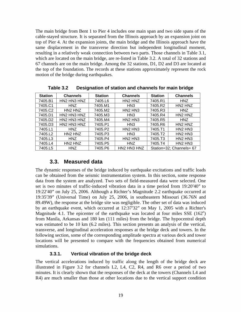
3.3.1. Vertical vibration of the bridge deck The vertical accelerations induced by traffic along the length of the bridge deck are illustrated in Figure 3.2 for channels L2, L4, C2, R4, and R6 over a period of two minutes. It is clearly shown that the responses of the deck at the towers (Channels L4 and R4) are much smaller than those at other locations due to the vertical support condition

19

by the towers. Although it is difficult without video images of the traffic condition to identify the vehicles that resulted in the deck vibration, three distinct events likely occurred as marked by numbered dashed lines in Figure 3.2. The north side of the bridge deck carries the westbound traffic on the state highway 74 as directed by the dashed lines. If a car or truck was driven at 50–100 km/h, the time required to move the vehicle from R6 to L2 is approximately 18–36 sec., which is consistent with the slope of the 3 dashed lines in Figure 3.2. It is speculated that, along the first path, a group of cars drove through the middle of the east side span at approximately 43 sec. and arrived at the middle of the west side span at 65 sec. Along the third path, a heavy truck may have driven through the bridge at a slightly slower speed. Another group of cars may have driven through the bridge at a continuously reduced speed along the second path. The acceleration on the north side of the deck may also be somewhat affected by the eastbound traffic along the south side of the bridge deck.

(a) North side of deck at middle of west side span (L2)

(b) North side of deck at Pier 2 (L4)

(c) North side of deck at middle of main span (C2)

(d) North side of deck at Pier 3 (R4)

1 3 2

(e) North side of deck at middle of east side span (R6)

Figure 3.2 Vertical accelerations at deck under traffic loading For the May 1, 2005 earthquake, the time histories are shown in Figure 3.3. From the top to bottom, the acceleration responses shown in Figure 3.3 are for channels L3, L5, C1, R1, and R3, respectively. Since the L3 and R3 channels are at the deck near the supports, their responses are significantly smaller than those of L5, C1, and R1.

20

(a) South side of deck at support of Pier 2 (L3)

(b) South side of deck at ¼ west of main span (L5)

(c) South side of deck at middle of main span (C1)

(d) South side of deck at ¼ east of main span (R1)

(e) South side of deck at support of Pier 3 (R3)

Figure 3.3 Vertical accelerations at deck under earthquake excitation

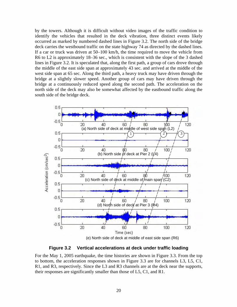
3.3.2. Transverse vibration Traffic-induced vibration is weak, particularly in the longitudinal and transverse directions, and also has a limited bandwidth. Therefore, some of the vibration modes may not be triggered by traffic loading. To see the general variation of the lateral vibration, Figure 3.4 shows the lateral accelerations at the top and middle of the towers at Piers 2 and 3. The vibration at the top is shown to be significantly stronger than that at the middle of tower. Both are weaker than the vertical vibration at the bridge deck presented in Figure 3.2.

21

(a) Top of tower at Pier 2 (b) Top of tower at Pier 3

(c) Middle of tower at Pier 2 (d) Middle of tower at Pier 3

Figure 3.4 Lateral accelerations at towers under traffic loading

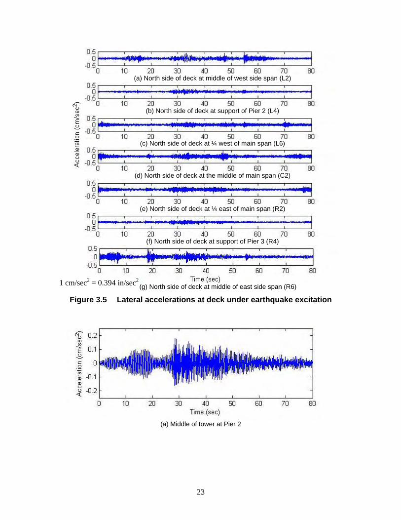
The acceleration responses for channels L2, L4, L6, C2, R2, R4, and R6 under the earthquake excitation are shown in Figure 3.5. Note that the responses at L4 and R4 are smaller than those at other channels since L4 and R4 are located at top of the lateral support by the towers.

Figure 3.6 presents the seismic acceleration time histories of the towers at M2 and M4. As seen from Figure 3.6, the peak values of the transverse accelerations at M2 and M4 are less than 0.2 cm/sec2 (0.0788 in/sec2). The vibration of the tower is not as strong as the bridge deck since the tower is much stiffer than the bridge deck.

3.3.3. Longitudinal vibration of the bridge tower The traffic-induced longitudinal accelerations at the top of two towers are shown in Figure 3.7. The maximum vibration levels are clearly similar at two sides of each tower but quite different between the towers due to passage of vehicular traffic. Overall, longitudinal vibration is small in comparison with the vertical vibration in the bridge deck as shown in Figure 3.2.

22

(a) North side of deck at middle of west side span (L2)

(b) North side of deck at support of Pier 2 (L4)

(c) North side of deck at ¼ west of main span (L6)

(d) North side of deck at the middle of main span (C2)

(e) North side of deck at ¼ east of main span (R2)

(f) North side of deck at support of Pier 3 (R4)

(g) North side of deck at middle of east side span (R6) 1 cm/sec2 = 0.394 in/sec2

Figure 3.5 Lateral accelerations at deck under earthquake excitation

(a) Middle of tower at Pier 2

23

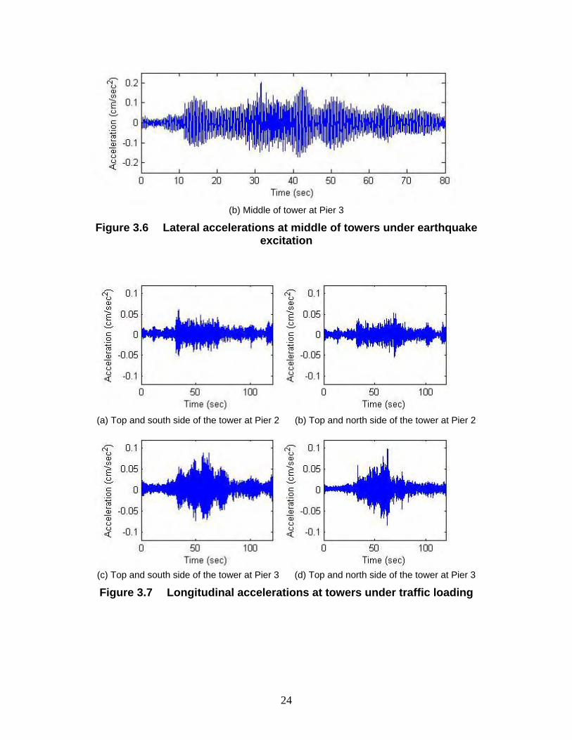
(b) Middle of tower at Pier 3

Figure 3.6 Lateral accelerations at middle of towers under earthquake excitation

(a) Top and south side of the tower at Pier 2 (b) Top and north side of the tower at Pier 2

(c) Top and south side of the tower at Pier 3 (d) Top and north side of the tower at Pier 3

Figure 3.7 Longitudinal accelerations at towers under traffic loading

24

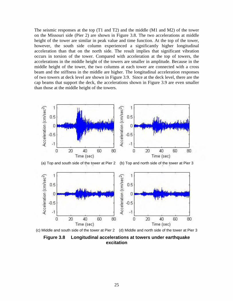
The seismic responses at the top (T1 and T2) and the middle (M1 and M2) of the tower on the Missouri side (Pier 2) are shown in Figure 3.8. The two accelerations at middle height of the tower are similar in peak value and time function. At the top of the tower, however, the south side column experienced a significantly higher longitudinal acceleration than that on the north side. The result implies that significant vibration occurs in torsion of the tower. Compared with acceleration at the top of towers, the accelerations in the middle height of the towers are smaller in amplitude. Because in the middle height of the tower, the two columns at each tower are connected with a cross beam and the stiffness in the middle are higher. The longitudinal acceleration responses of two towers at deck level are shown in Figure 3.9. Since at the deck level, there are the cap beams that support the deck, the accelerations shown in Figure 3.9 are even smaller than those at the middle height of the towers.

(a) Top and south side of the tower at Pier 2 (b) Top and north side of the tower at Pier 3

(c) Middle and south side of the tower at Pier 2 (d) Middle and north side of the tower at Pier 3

Figure 3.8 Longitudinal accelerations at towers under earthquake excitation

25

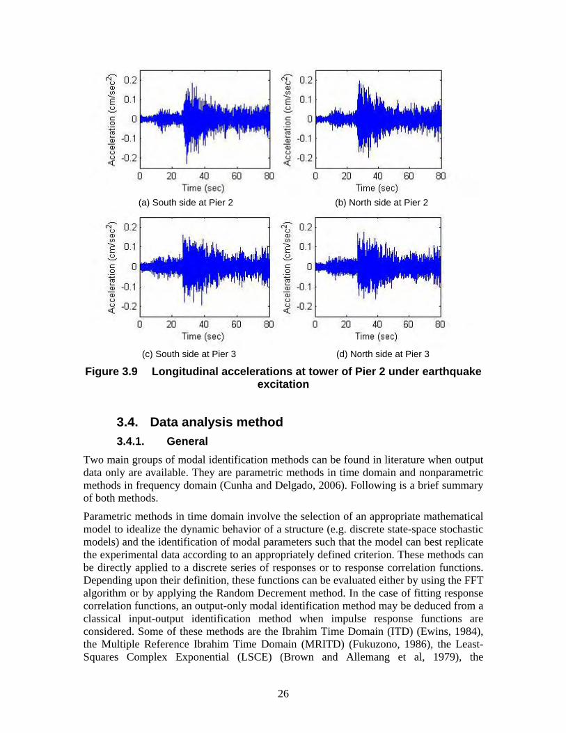
(a) South side at Pier 2 (b) North side at Pier 2

(c) South side at Pier 3 (d) North side at Pier 3

Figure 3.9 Longitudinal accelerations at tower of Pier 2 under earthquake excitation

3.4. Data analysis method 3.4.1. General

Two main groups of modal identification methods can be found in literature when output data only are available. They are parametric methods in time domain and nonparametric methods in frequency domain (Cunha and Delgado, 2006). Following is a brief summary of both methods.

Parametric methods in time domain involve the selection of an appropriate mathematical model to idealize the dynamic behavior of a structure (e.g. discrete state-space stochastic models) and the identification of modal parameters such that the model can best replicate the experimental data according to an appropriately defined criterion. These methods can be directly applied to a discrete series of responses or to response correlation functions. Depending upon their definition, these functions can be evaluated either by using the FFT algorithm or by applying the Random Decrement method. In the case of fitting response correlation functions, an output-only modal identification method may be deduced from a classical input-output identification method when impulse response functions are considered. Some of these methods are the Ibrahim Time Domain (ITD) (Ewins, 1984), the Multiple Reference Ibrahim Time Domain (MRITD) (Fukuzono, 1986), the Least-Squares Complex Exponential (LSCE) (Brown and Allemang et al, 1979), the

26

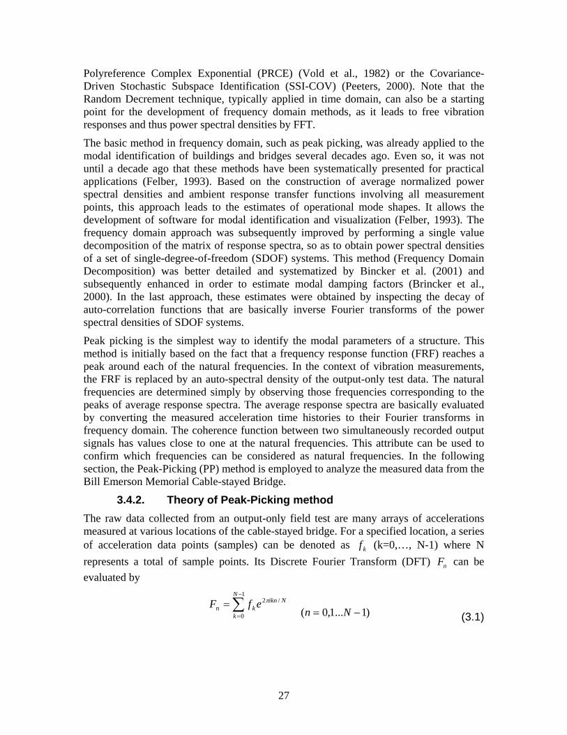
Polyreference Complex Exponential (PRCE) (Vold et al., 1982) or the Covariance-Driven Stochastic Subspace Identification (SSI-COV) (Peeters, 2000). Note that the Random Decrement technique, typically applied in time domain, can also be a starting point for the development of frequency domain methods, as it leads to free vibration responses and thus power spectral densities by FFT.

The basic method in frequency domain, such as peak picking, was already applied to the modal identification of buildings and bridges several decades ago. Even so, it was not until a decade ago that these methods have been systematically presented for practical applications (Felber, 1993). Based on the construction of average normalized power spectral densities and ambient response transfer functions involving all measurement points, this approach leads to the estimates of operational mode shapes. It allows the development of software for modal identification and visualization (Felber, 1993). The frequency domain approach was subsequently improved by performing a single value decomposition of the matrix of response spectra, so as to obtain power spectral densities of a set of single-degree-of-freedom (SDOF) systems. This method (Frequency Domain Decomposition) was better detailed and systematized by Bincker et al. (2001) and subsequently enhanced in order to estimate modal damping factors (Brincker et al., 2000). In the last approach, these estimates were obtained by inspecting the decay of auto-correlation functions that are basically inverse Fourier transforms of the power spectral densities of SDOF systems.

Peak picking is the simplest way to identify the modal parameters of a structure. This method is initially based on the fact that a frequency response function (FRF) reaches a peak around each of the natural frequencies. In the context of vibration measurements, the FRF is replaced by an auto-spectral density of the output-only test data. The natural frequencies are determined simply by observing those frequencies corresponding to the peaks of average response spectra. The average response spectra are basically evaluated by converting the measured acceleration time histories to their Fourier transforms in frequency domain. The coherence function between two simultaneously recorded output signals has values close to one at the natural frequencies. This attribute can be used to confirm which frequencies can be considered as natural frequencies. In the following section, the Peak-Picking (PP) method is employed to analyze the measured data from the Bill Emerson Memorial Cable-stayed Bridge.

3.4.2. Theory of Peak-Picking method The raw data collected from an output-only field test are many arrays of accelerations measured at various locations of the cable-stayed bridge. For a specified location, a series of acceleration data points (samples) can be denoted as f k (k=0,…, N-1) where N represents a total of sample points. Its Discrete Fourier Transform (DFT) F can be evaluated by

n

N 1

= ∑−

F 2 ikn / Nn f k e π

k =0 (n = 0,1...N −1) (3.1)

27

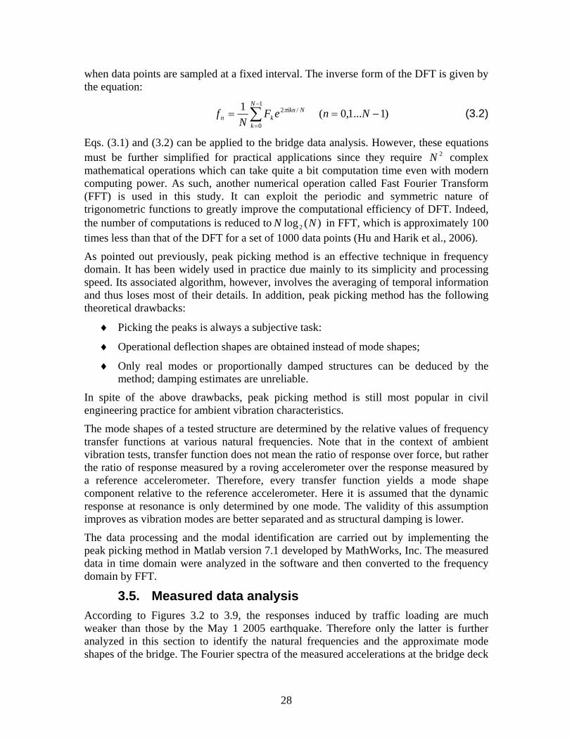
when data points are sampled at a fixed interval. The inverse form of the DFT is given by the equation:

1 N −1

f = 2 ikn / Nn ∑ Fk e π (n = 0,1...N −1) (3.2)

N k =0

Eqs. (3.1) and (3.2) can be applied to the bridge data analysis. However, these equations must be further simplified for practical applications since they require N 2 complex mathematical operations which can take quite a bit computation time even with modern computing power. As such, another numerical operation called Fast Fourier Transform (FFT) is used in this study. It can exploit the periodic and symmetric nature of trigonometric functions to greatly improve the computational efficiency of DFT. Indeed, the number of computations is reduced to N log2 (N ) in FFT, which is approximately 100 times less than that of the DFT for a set of 1000 data points (Hu and Harik et al., 2006).

As pointed out previously, peak picking method is an effective technique in frequency domain. It has been widely used in practice due mainly to its simplicity and processing speed. Its associated algorithm, however, involves the averaging of temporal information and thus loses most of their details. In addition, peak picking method has the following theoretical drawbacks:

♦

♦

♦

Picking the peaks is always a subjective task:

Operational deflection shapes are obtained instead of mode shapes;

Only real modes or proportionally damped structures can be deduced by the method; damping estimates are unreliable.

In spite of the above drawbacks, peak picking method is still most popular in civil engineering practice for ambient vibration characteristics.

The mode shapes of a tested structure are determined by the relative values of frequency transfer functions at various natural frequencies. Note that in the context of ambient vibration tests, transfer function does not mean the ratio of response over force, but rather the ratio of response measured by a roving accelerometer over the response measured by a reference accelerometer. Therefore, every transfer function yields a mode shape component relative to the reference accelerometer. Here it is assumed that the dynamic response at resonance is only determined by one mode. The validity of this assumption improves as vibration modes are better separated and as structural damping is lower.

The data processing and the modal identification are carried out by implementing the peak picking method in Matlab version 7.1 developed by MathWorks, Inc. The measured data in time domain were analyzed in the software and then converted to the frequency domain by FFT.

3.5. Measured data analysis According to Figures 3.2 to 3.9, the responses induced by traffic loading are much weaker than those by the May 1 2005 earthquake. Therefore only the latter is further analyzed in this section to identify the natural frequencies and the approximate mode shapes of the bridge. The Fourier spectra of the measured accelerations at the bridge deck

28

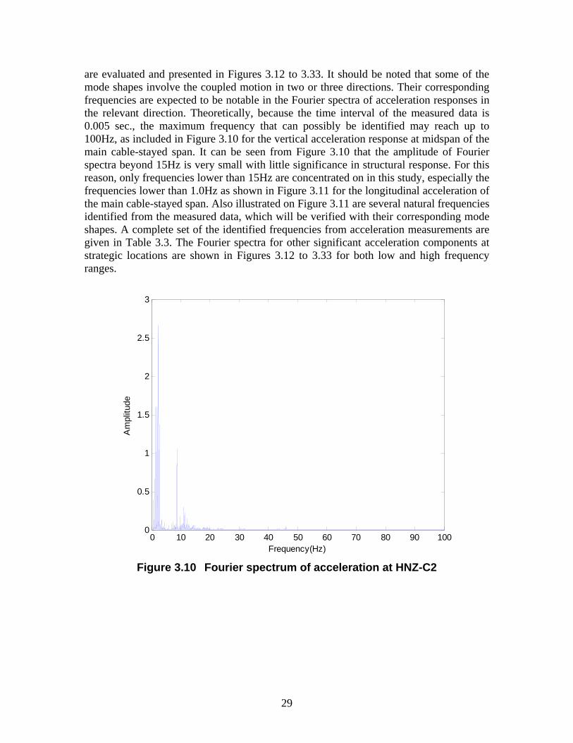
are evaluated and presented in Figures 3.12 to 3.33. It should be noted that some of the mode shapes involve the coupled motion in two or three directions. Their corresponding frequencies are expected to be notable in the Fourier spectra of acceleration responses in the relevant direction. Theoretically, because the time interval of the measured data is 0.005 sec., the maximum frequency that can possibly be identified may reach up to 100Hz, as included in Figure 3.10 for the vertical acceleration response at midspan of the main cable-stayed span. It can be seen from Figure 3.10 that the amplitude of Fourier spectra beyond 15Hz is very small with little significance in structural response. For this reason, only frequencies lower than 15Hz are concentrated on in this study, especially the frequencies lower than 1.0Hz as shown in Figure 3.11 for the longitudinal acceleration of the main cable-stayed span. Also illustrated on Figure 3.11 are several natural frequencies identified from the measured data, which will be verified with their corresponding mode shapes. A complete set of the identified frequencies from acceleration measurements are given in Table 3.3. The Fourier spectra for other significant acceleration components at strategic locations are shown in Figures 3.12 to 3.33 for both low and high frequency ranges.

0 10 20 30 40 50 60 70 80 90 1000

0.5

1

1.5

2

2.5

3

Frequency(Hz)

Am

plitu

de

Figure 3.10 Fourier spectrum of acceleration at HNZ-C2

29

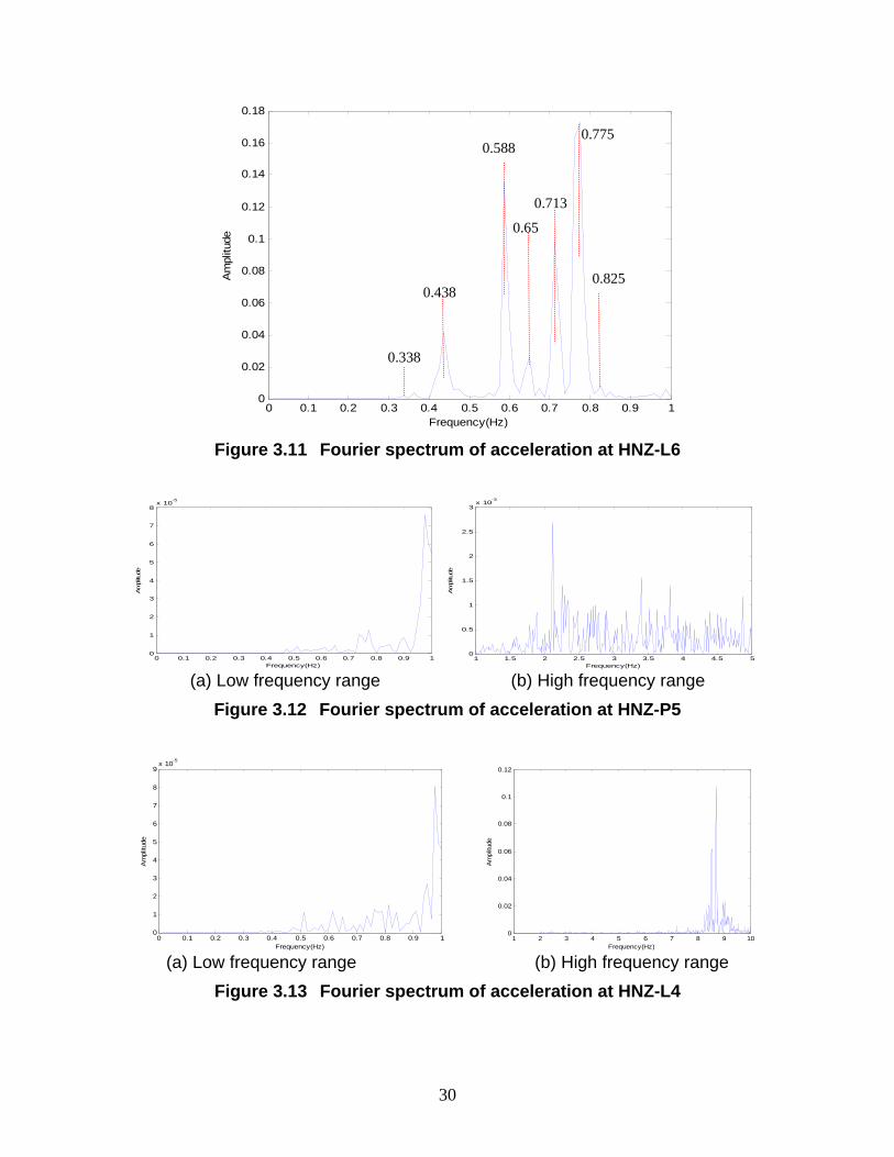
0.18

0 0.1 0.2 0.3 0.4 0.5 0.6 0.7 0.8 0.9 10

0.02

0.04

0.06

0.08

0.1

0.12

0.14

0.16

Frequency(Hz)

Am

plitu

de

0.338

0.438

0.588

0.65

0.713

0.775

0.825

Figure 3.11 Fourier spectrum of acceleration at HNZ-L6

1 1.5 2 2.5 3 3.5 4 4.5 50

0.5

1

1.5

2

2.5

3x 10-3

Frequency(Hz)

Am

plitu

de

0 0.1 0.2 0.3 0.4 0.5 0.6 0.7 0.8 0.9 10

1

2

3

4

5

6

7

8x 10-5

Frequency(Hz)

Am

plitu

de

(a) Low frequency range (b) High frequency range

Figure 3.12 Fourier spectrum of acceleration at HNZ-P5

0 0.1 0.2 0.3 0.4 0.5 0.6 0.7 0.8 0.9 10

1

2

3

4

5

6

7

8

9x 10-5

Frequency(Hz)

Am

plitu

de

1 2 3 4 5 6 7 8 9 100

0.02

0.04

0.06

0.08

0.1

0.12

Frequency(Hz)

Am

plitu

de

(a) Low frequency range (b) High frequency range

Figure 3.13 Fourier spectrum of acceleration at HNZ-L4

30

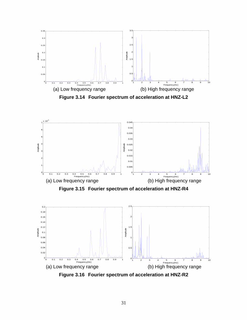
1 2 3 4 5 6 7 8 9 100

0.5

1

1.5

2

2.5

3

3.5

Frequency(Hz)

Am

plitu

de

0 0.1 0.2 0.3 0.4 0.5 0.6 0.7 0.8 0.9 10

0.05

0.1

0.15

0.2

0.25

0.3

0.35

Frequency(Hz)

Am

plitu

de

(a) Low frequency range (b) High frequency range

Figure 3.14 Fourier spectrum of acceleration at HNZ-L2

0 0.1 0.2 0.3 0.4 0.5 0.6 0.7 0.8 0.9 10

1

2

3

4

5

6

7x 10-5

Frequency(Hz)

Am

plitu

de

1 2 3 4 5 6 7 8 9 100

0.005

0.01

0.015

0.02

0.025

0.03

0.035

0.04

0.045

Frequency(Hz)

Am

plitu

de

(a) Low frequency range (b) High frequency range

Figure 3.15 Fourier spectrum of acceleration at HNZ-R4

1 2 3 4 5 6 7 8 9 100

0.5

1

1.5

2

2.5

Frequency(Hz)

Am

plitu

de

0 0.1 0.2 0.3 0.4 0.5 0.6 0.7 0.8 0.9 10

0.02

0.04

0.06

0.08

0.1

0.12

0.14

0.16

0.18

0.2

Frequency(Hz)

Am

plitu

de

(a) Low frequency range (b) High frequency range

Figure 3.16 Fourier spectrum of acceleration at HNZ-R2

31

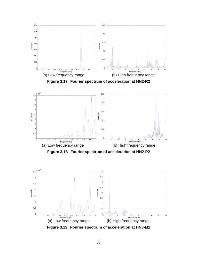
0 0.1 0.2 0.3 0.4 0.5 0.6 0.7 0.8 0.9 10

0.02

0.04

0.06

0.08

0.1

0.12

0.14

Frequency(Hz)

Am

plitu

de

1 2 3 4 5 6 7 8 9 100

0.05

0.1

0.15

0.2

0.25

Frequency(Hz)

Am

plitu

de

(a) Low frequency range (b) High frequency range

Figure 3.17 Fourier spectrum of acceleration at HN2-R2

0 0.1 0.2 0.3 0.4 0.5 0.6 0.7 0.8 0.9 10

0.5

1

1.5

2

2.5

3

3.5

4

4.5x 10-5

Frequency(Hz)

Am

plitu

de

1 2 3 4 5 6 7 8 9 100

0.05

0.1

0.15

0.2

0.25

Frequency(Hz)

Am

plitu

de

(a) Low frequency range (b) High frequency range

Figure 3.18 Fourier spectrum of acceleration at HN2-P2

0 0.1 0.2 0.3 0.4 0.5 0.6 0.7 0.8 0.9 10

0.5

1

1.5

2

2.5

3

3.5x 10-3

Frequency(Hz)

Am

plitu

de

1 2 3 4 5 6 7 8 9 100

0.5

1

1.5

2

2.5

3

3.5

4

Frequency(Hz)

Am

plitu

de

(a) Low frequency range (b) High frequency range Figure 3.19 Fourier spectrum of acceleration at HN3-M2

32

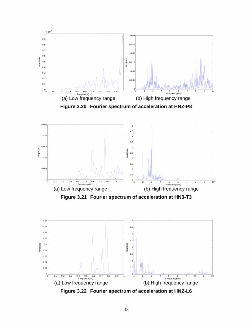
0 0.1 0.2 0.3 0.4 0.5 0.6 0.7 0.8 0.9 10

0.1

0.2

0.3

0.4

0.5

0.6

0.7

0.8

0.9

1x 10-4

Frequency(Hz)

Am

plitu

de

1 2 3 4 5 6 7 8 9 100

0.005

0.01

0.015

0.02

0.025

0.03

Frequency(Hz)

Am

plitu

de

(a) Low frequency range (b) High frequency range

Figure 3.20 Fourier spectrum of acceleration at HNZ-P8

0 0.1 0.2 0.3 0.4 0.5 0.6 0.7 0.8 0.9 10

0.005

0.01

0.015

0.02

0.025

Frequency(Hz)

Am

plitu

de

1 2 3 4 5 6 7 8 9 100

0.5

1

1.5

2

2.5

3

3.5

4

4.5

5

Frequency(Hz)

Am

plitu

de

(a) Low frequency range (b) High frequency range

Figure 3.21 Fourier spectrum of acceleration at HN3-T3

1 2 3 4 5 6 7 8 9 100

0.5

1

1.5

2

2.5

3

3.5

4

Frequency(Hz)

Am

plitu

de

0 0.1 0.2 0.3 0.4 0.5 0.6 0.7 0.8 0.9 10

0.02

0.04

0.06

0.08

0.1

0.12

0.14

0.16

0.18

Frequency(Hz)

Am

plitu

de

(a) Low frequency range (b) High frequency range

Figure 3.22 Fourier spectrum of acceleration at HNZ-L6

33

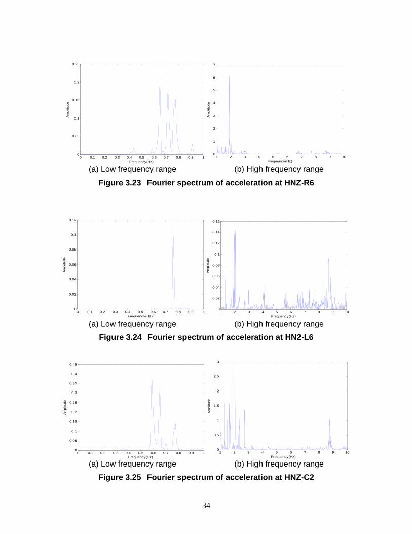
0 0.1 0.2 0.3 0.4 0.5 0.6 0.7 0.8 0.9 10

0.05

0.1

0.15

0.2

0.25

Frequency(Hz)

Am

plitu

de

1 2 3 4 5 6 7 8 9 100

1

2

3

4

5

6

7

Frequency(Hz)

Am

plitu

de

(a) Low frequency range (b) High frequency range

Figure 3.23 Fourier spectrum of acceleration at HNZ-R6

0 0.1 0.2 0.3 0.4 0.5 0.6 0.7 0.8 0.9 10

0.02

0.04

0.06

0.08

0.1

0.12

Frequency(Hz)

Am

plitu

de

1 2 3 4 5 6 7 8 9 100

0.02

0.04

0.06

0.08

0.1

0.12

0.14

0.16

Frequency(Hz)

Am

plitu

de

(a) Low frequency range (b) High frequency range

Figure 3.24 Fourier spectrum of acceleration at HN2-L6

1 2 3 4 5 6 7 8 9 100

0.5

1

1.5

2

2.5

3

Frequency(Hz)

Am

plitu

de

0 0.1 0.2 0.3 0.4 0.5 0.6 0.7 0.8 0.9 10

0.05

0.1

0.15

0.2

0.25

0.3

0.35

0.4

0.45

Frequency(Hz)

Am

plitu

de

(a) Low frequency range (b) High frequency range

Figure 3.25 Fourier spectrum of acceleration at HNZ-C2

34

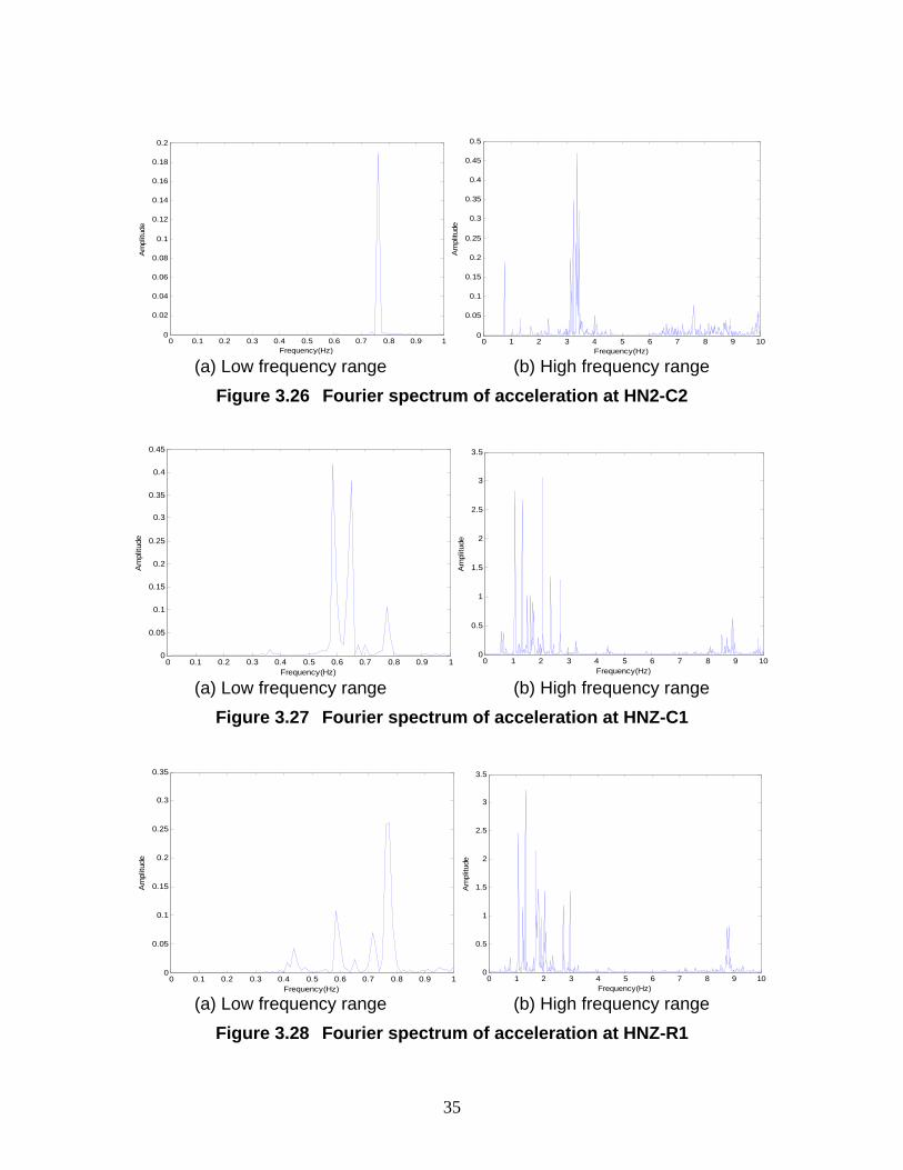
0 1 2 3 4 5 6 7 8 9 100

0.05

0.1

0.15

0.2

0.25

0.3

0.35

0.4

0.45

0.5

Frequency(Hz)

Am

plitu

de

0 0.1 0.2 0.3 0.4 0.5 0.6 0.7 0.8 0.9 10

0.02

0.04

0.06

0.08

0.1

0.12

0.14

0.16

0.18

0.2

Frequency(Hz)

Am

plitu

de

(a) Low frequency range (b) High frequency range

Figure 3.26 Fourier spectrum of acceleration at HN2-C2

0 0.1 0.2 0.3 0.4 0.5 0.6 0.7 0.8 0.9 10

0.05

0.1

0.15

0.2

0.25

0.3

0.35

0.4

0.45

Frequency(Hz)

Am

plitu

de

0 1 2 3 4 5 6 7 8 9 100

0.5

1

1.5

2

2.5

3

3.5

Frequency(Hz)

Am

plitu

de

(a) Low frequency range (b) High frequency range

Figure 3.27 Fourier spectrum of acceleration at HNZ-C1

0 0.1 0.2 0.3 0.4 0.5 0.6 0.7 0.8 0.9 10

0.05

0.1

0.15

0.2

0.25

0.3

0.35

Frequency(Hz)

Am

plitu

de

0 1 2 3 4 5 6 7 8 9 100

0.5

1

1.5

2

2.5

3

3.5

Frequency(Hz)

Am

plitu

de

(a) Low frequency range (b) High frequency range

Figure 3.28 Fourier spectrum of acceleration at HNZ-R1

35

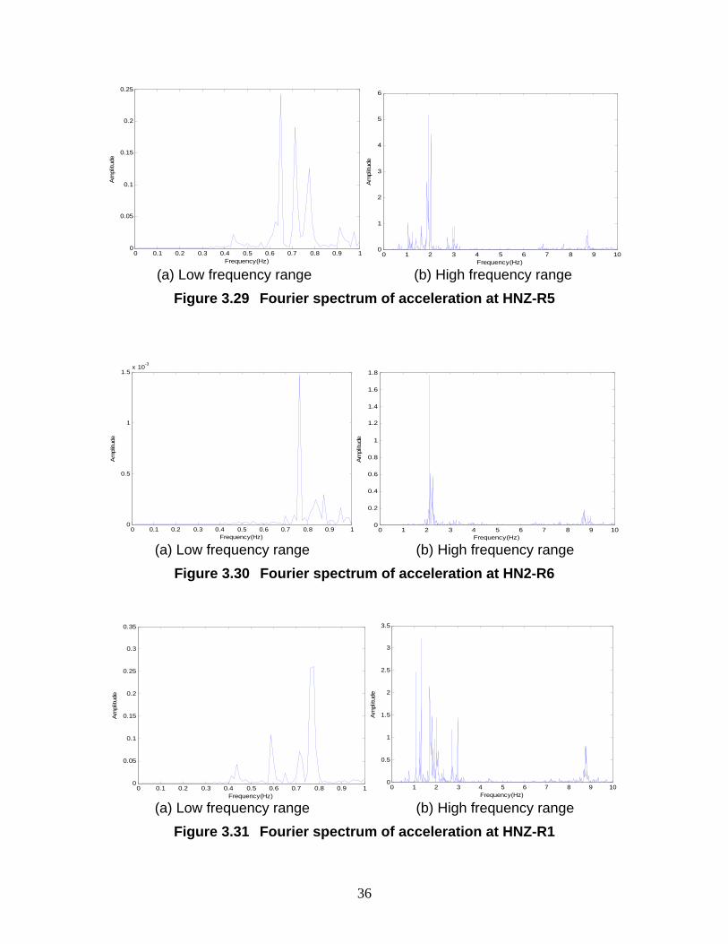
0 0.1 0.2 0.3 0.4 0.5 0.6 0.7 0.8 0.9 10

0.05

0.1

0.15

0.2

0.25

Frequency(Hz)

Am

plitu

de

0 1 2 3 4 5 6 7 8 9 100

1

2

3

4

5

6

Frequency(Hz)

Am

plitu

de

(a) Low frequency range (b) High frequency range

Figure 3.29 Fourier spectrum of acceleration at HNZ-R5

0 0.1 0.2 0.3 0.4 0.5 0.6 0.7 0.8 0.9 10

0.5

1

1.5x 10-3

Frequency(Hz)

Am

plitu

de

0 1 2 3 4 5 6 7 8 9 100

0.2

0.4

0.6

0.8

1

1.2

1.4

1.6

1.8

Frequency(Hz)

Am

plitu

de

(a) Low frequency range (b) High frequency range

Figure 3.30 Fourier spectrum of acceleration at HN2-R6

0 1 2 3 4 5 6 7 8 9 100

0.5

1

1.5

2

2.5

3

3.5

Frequency(Hz)

Am

plitu

de

0 0.1 0.2 0.3 0.4 0.5 0.6 0.7 0.8 0.9 10

0.05

0.1

0.15

0.2

0.25

0.3

0.35

Frequency(Hz)

Am

plitu

de

(a) Low frequency range (b) High frequency range

Figure 3.31 Fourier spectrum of acceleration at HNZ-R1

36

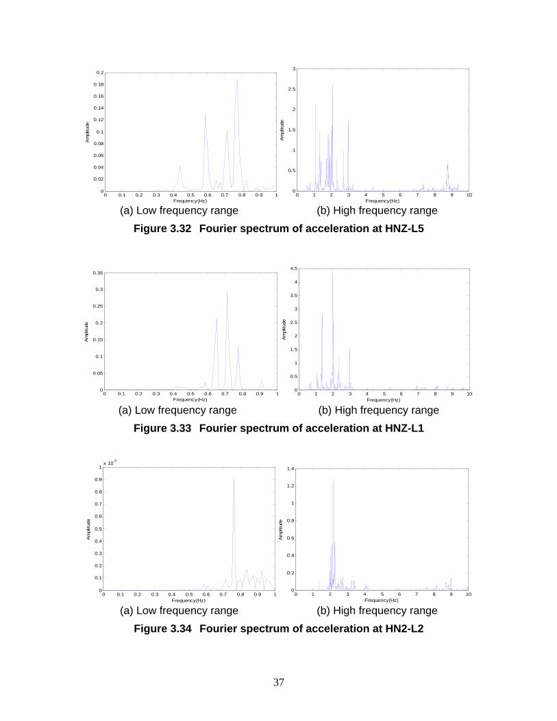
0 1 2 3 4 5 6 7 8 9 100

0.5

1

1.5

2

2.5

3

Frequency(Hz)

Am

plitu

de

0 0.1 0.2 0.3 0.4 0.5 0.6 0.7 0.8 0.9 10

0.02

0.04

0.06

0.08

0.1

0.12

0.14

0.16

0.18

0.2

Frequency(Hz)

Am

plitu

de

(a) Low frequency range (b) High frequency range

Figure 3.32 Fourier spectrum of acceleration at HNZ-L5

0 1 2 3 4 5 6 7 8 9 100

0.5

1

1.5

2

2.5

3

3.5

4

4.5

Frequency(Hz)

Am

plitu

de

0 0.1 0.2 0.3 0.4 0.5 0.6 0.7 0.8 0.9 10

0.05

0.1

0.15

0.2

0.25

0.3

0.35

Frequency(Hz)

Am

plitu

de

(a) Low frequency range (b) High frequency range

Figure 3.33 Fourier spectrum of acceleration at HNZ-L1

0 0.1 0.2 0.3 0.4 0.5 0.6 0.7 0.8 0.9 10

0.1

0.2

0.3

0.4

0.5

0.6

0.7

0.8

0.9

1x 10-3

Frequency(Hz)

Am

plitu

de

0 1 2 3 4 5 6 7 8 9 100

0.2

0.4

0.6

0.8

1

1.2

1.4

Frequency(Hz)

Am

plitu

de

(a) Low frequency range (b) High frequency range

Figure 3.34 Fourier spectrum of acceleration at HN2-L2

37

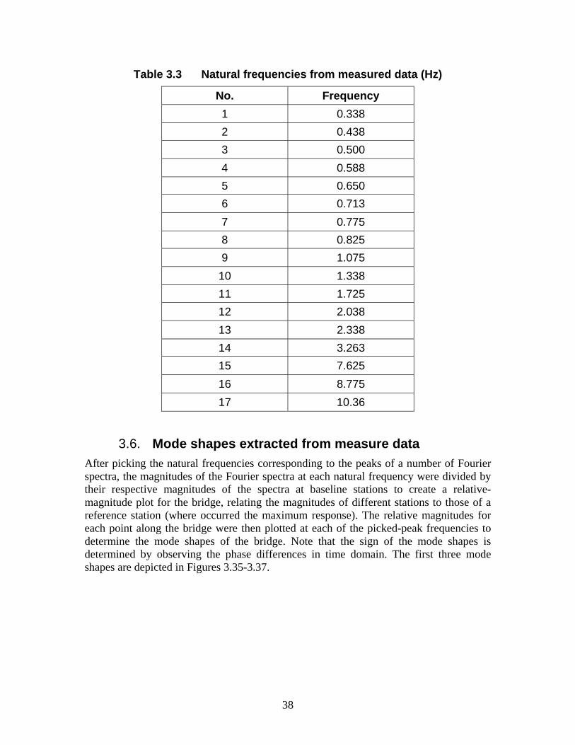
Table 3.3 Natural frequencies from measured data (Hz)

No. Frequency1 0.3382 0.4383 0.5004 0.5885 0.6506 0.7137 0.7758 0.8259 1.07510 1.33811 1.72512 2.03813 2.33814 3.26315 7.62516 8.77517 10.36

3.6. Mode shapes extracted from measure data After picking the natural frequencies corresponding to the peaks of a number of Fourier spectra, the magnitudes of the Fourier spectra at each natural frequency were divided by their respective magnitudes of the spectra at baseline stations to create a relative-magnitude plot for the bridge, relating the magnitudes of different stations to those of a reference station (where occurred the maximum response). The relative magnitudes for each point along the bridge were then plotted at each of the picked-peak frequencies to determine the mode shapes of the bridge. Note that the sign of the mode shapes is determined by observing the phase differences in time domain. The first three mode shapes are depicted in Figures 3.35-3.37.

38

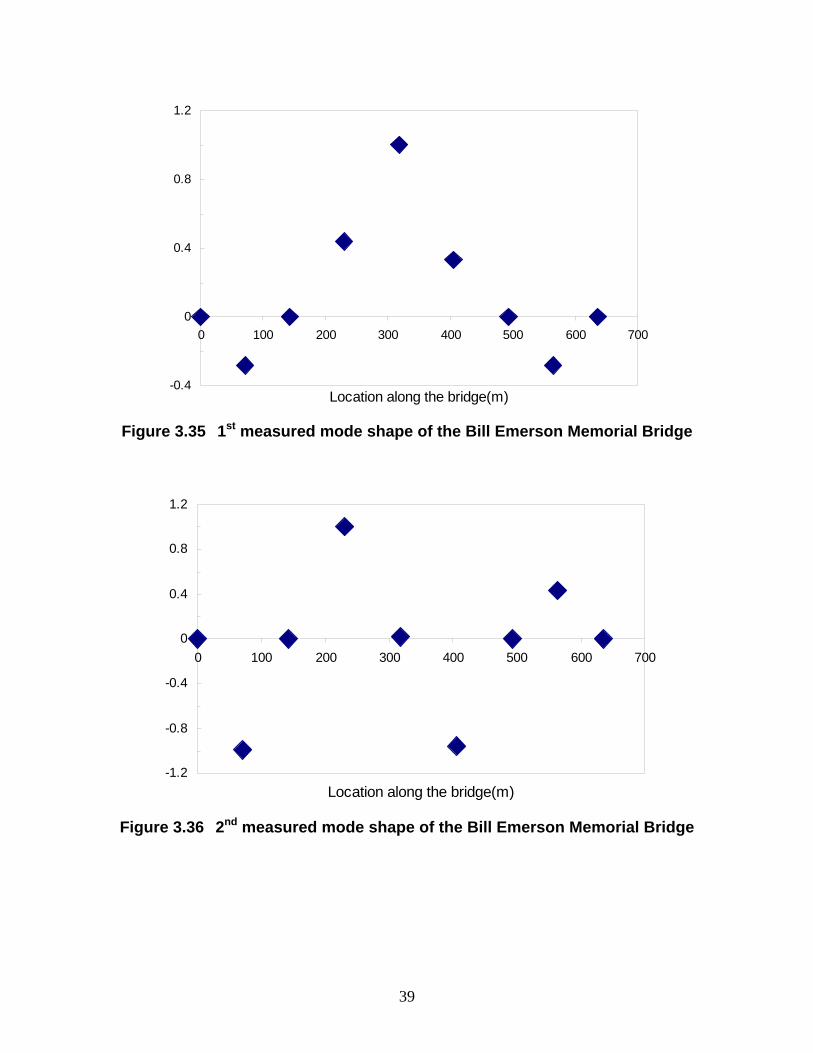
-0.4

0

0.4

0.8

1.2

0 100 200 300 400 500 600 700

Location along the bridge(m)

stFigure 3.35 1 measured mode shape of the Bill Emerson Memorial Bridge

-1.2

-0.8

-0.4

0

0.4

0.8

1.2

0 100 200 300 400 500 600 700

Location along the bridge(m)

ndFigure 3.36 2 measured mode shape of the Bill Emerson Memorial Bridge

39

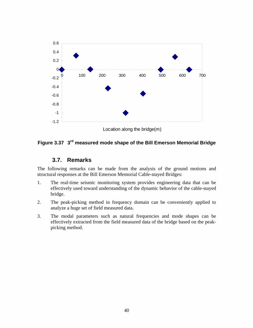
-1.2

-1

-0.8

-0.6

-0.4

-0.2

0

0.2

0.4

0.6

0 100 200 300 400 500 600 700

Location along the bridge(m)

rdFigure 3.37 3 measured mode shape of the Bill Emerson Memorial Bridge

3.7. Remarks The following remarks can be made from the analysis of the ground motions and structural responses at the Bill Emerson Memorial Cable-stayed Bridges:

1. The real-time seismic monitoring system provides engineering data that can be effectively used toward understanding of the dynamic behavior of the cable-stayed bridge.

2. The peak-picking method in frequency domain can be conveniently applied to analyze a huge set of field measured data.

3. The modal parameters such as natural frequencies and mode shapes can be effectively extracted from the field measured data of the bridge based on the peak-picking method.

40

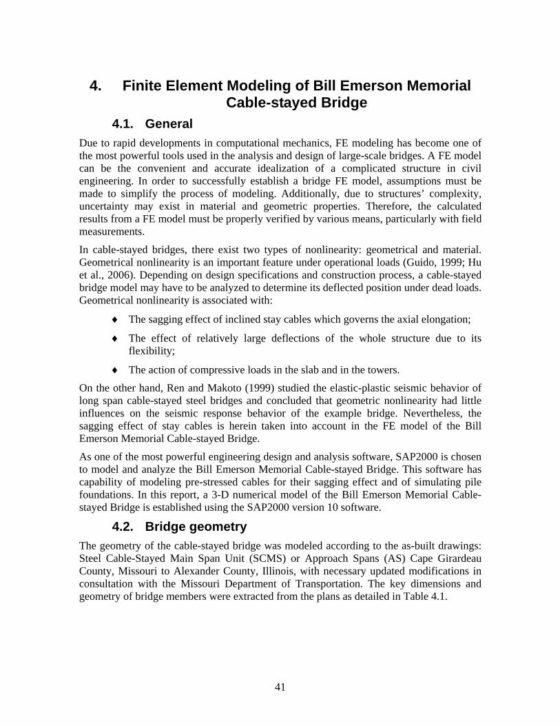
4. Finite Element Modeling of Bill Emerson Memorial Cable-stayed Bridge

4.1. General Due to rapid developments in computational mechanics, FE modeling has become one of the most powerful tools used in the analysis and design of large-scale bridges. A FE model can be the convenient and accurate idealization of a complicated structure in civil engineering. In order to successfully establish a bridge FE model, assumptions must be made to simplify the process of modeling. Additionally, due to structures’ complexity, uncertainty may exist in material and geometric properties. Therefore, the calculated results from a FE model must be properly verified by various means, particularly with field measurements.

In cable-stayed bridges, there exist two types of nonlinearity: geometrical and material. Geometrical nonlinearity is an important feature under operational loads (Guido, 1999; Hu et al., 2006). Depending on design specifications and construction process, a cable-stayed bridge model may have to be analyzed to determine its deflected position under dead loads. Geometrical nonlinearity is associated with:

♦

♦

♦

The sagging effect of inclined stay cables which governs the axial elongation;

The effect of relatively large deflections of the whole structure due to its flexibility;

The action of compressive loads in the slab and in the towers.

On the other hand, Ren and Makoto (1999) studied the elastic-plastic seismic behavior of long span cable-stayed steel bridges and concluded that geometric nonlinearity had little influences on the seismic response behavior of the example bridge. Nevertheless, the sagging effect of stay cables is herein taken into account in the FE model of the Bill Emerson Memorial Cable-stayed Bridge.

As one of the most powerful engineering design and analysis software, SAP2000 is chosen to model and analyze the Bill Emerson Memorial Cable-stayed Bridge. This software has capability of modeling pre-stressed cables for their sagging effect and of simulating pile foundations. In this report, a 3-D numerical model of the Bill Emerson Memorial Cable-stayed Bridge is established using the SAP2000 version 10 software.

4.2. Bridge geometry The geometry of the cable-stayed bridge was modeled according to the as-built drawings: Steel Cable-Stayed Main Span Unit (SCMS) or Approach Spans (AS) Cape Girardeau County, Missouri to Alexander County, Illinois, with necessary updated modifications in consultation with the Missouri Department of Transportation. The key dimensions and geometry of bridge members were extracted from the plans as detailed in Table 4.1.

41

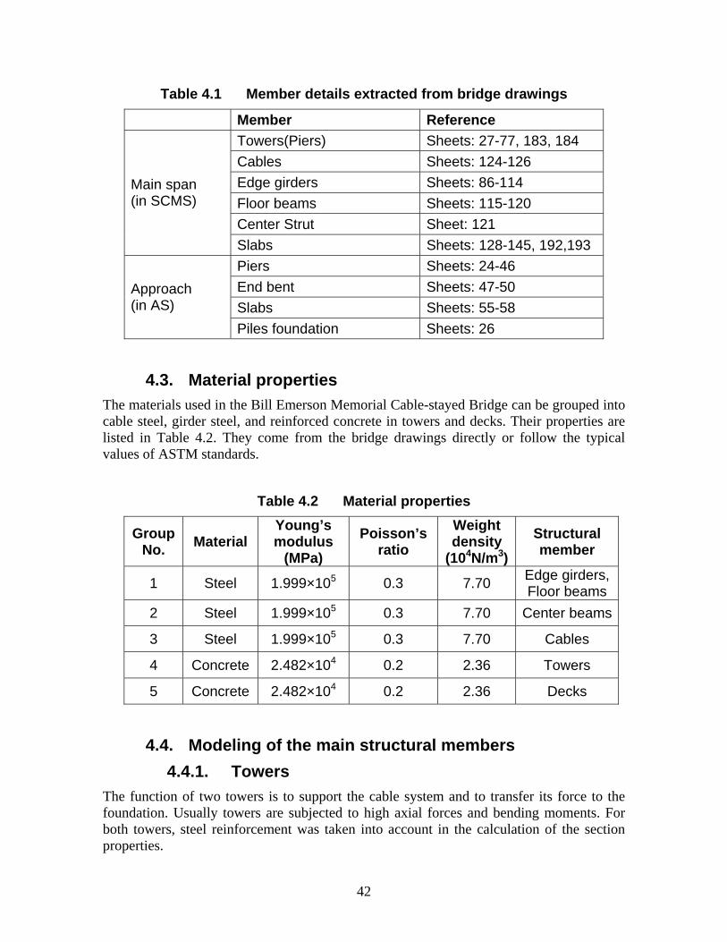
Table 4.1 Member details extracted from bridge drawings

Member Reference

Main span (in SCMS)

Towers(Piers) Sheets: 27-77, 183, 184 Cables Sheets: 124-126Edge girders Sheets: 86-114 Floor beams Sheets: 115-120 Center Strut Sheet: 121 Slabs Sheets: 128-145, 192,193

Approach (in AS)

Piers Sheets: 24-46End bent Sheets: 47-50 Slabs Sheets: 55-58Piles foundation Sheets: 26

4.3. Material properties The materials used in the Bill Emerson Memorial Cable-stayed Bridge can be grouped into cable steel, girder steel, and reinforced concrete in towers and decks. Their properties are listed in Table 4.2. They come from the bridge drawings directly or follow the typical values of ASTM standards.

Table 4.2 Material properties

Group No. Material

Young’s modulus

(MPa) Poisson’s

ratio Weight density

(104N/m3)Structural member

1 Steel 1.999×105 0.3 7.70 Edge girders, Floor beams

2 Steel 51.999×10 0.3 7.70 Center beams

3 Steel 51.999×10 0.3 7.70 Cables

4 Concrete 42.482×10 0.2 2.36 Towers

5 Concrete 42.482×10 0.2 2.36 Decks

4.4. Modeling of the main structural members 4.4.1. Towers

The function of two towers is to support the cable system and to transfer its force to the foundation. Usually towers are subjected to high axial forces and bending moments. For both towers, steel reinforcement was taken into account in the calculation of the section properties.

42

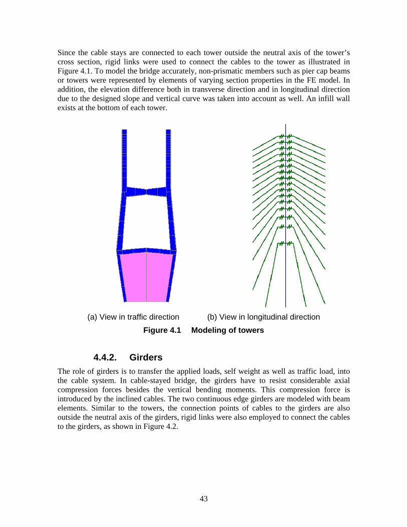
Since the cable stays are connected to each tower outside the neutral axis of the tower’s cross section, rigid links were used to connect the cables to the tower as illustrated in Figure 4.1. To model the bridge accurately, non-prismatic members such as pier cap beams or towers were represented by elements of varying section properties in the FE model. In addition, the elevation difference both in transverse direction and in longitudinal direction due to the designed slope and vertical curve was taken into account as well. An infill wall exists at the bottom of each tower.

(a) View in traffic direction (b) View in longitudinal direction

Figure 4.1 Modeling of towers

4.4.2. Girders The role of girders is to transfer the applied loads, self weight as well as traffic load, into the cable system. In cable-stayed bridge, the girders have to resist considerable axial compression forces besides the vertical bending moments. This compression force is introduced by the inclined cables. The two continuous edge girders are modeled with beam elements. Similar to the towers, the connection points of cables to the girders are also outside the neutral axis of the girders, rigid links were also employed to connect the cables to the girders, as shown in Figure 4.2.

43

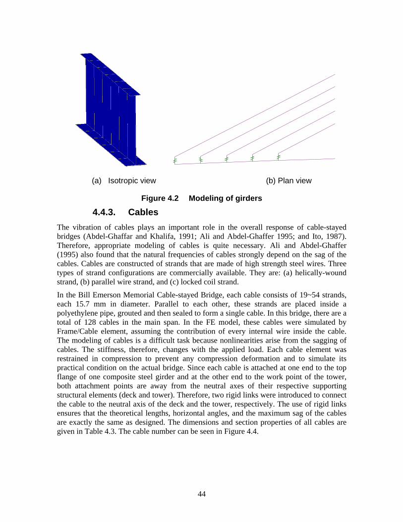
(a) Isotropic view (b) Plan view

Figure 4.2 Modeling of girders

4.4.3. Cables The vibration of cables plays an important role in the overall response of cable-stayed bridges (Abdel-Ghaffar and Khalifa, 1991; Ali and Abdel-Ghaffer 1995; and Ito, 1987). Therefore, appropriate modeling of cables is quite necessary. Ali and Abdel-Ghaffer (1995) also found that the natural frequencies of cables strongly depend on the sag of the cables. Cables are constructed of strands that are made of high strength steel wires. Three types of strand configurations are commercially available. They are: (a) helically-wound strand, (b) parallel wire strand, and (c) locked coil strand.

In the Bill Emerson Memorial Cable-stayed Bridge, each cable consists of 19~54 strands, each 15.7 mm in diameter. Parallel to each other, these strands are placed inside a polyethylene pipe, grouted and then sealed to form a single cable. In this bridge, there are a total of 128 cables in the main span. In the FE model, these cables were simulated by Frame/Cable element, assuming the contribution of every internal wire inside the cable. The modeling of cables is a difficult task because nonlinearities arise from the sagging of cables. The stiffness, therefore, changes with the applied load. Each cable element was restrained in compression to prevent any compression deformation and to simulate its practical condition on the actual bridge. Since each cable is attached at one end to the top flange of one composite steel girder and at the other end to the work point of the tower, both attachment points are away from the neutral axes of their respective supporting structural elements (deck and tower). Therefore, two rigid links were introduced to connect the cable to the neutral axis of the deck and the tower, respectively. The use of rigid links ensures that the theoretical lengths, horizontal angles, and the maximum sag of the cables are exactly the same as designed. The dimensions and section properties of all cables are given in Table 4.3. The cable number can be seen in Figure 4.4.

44

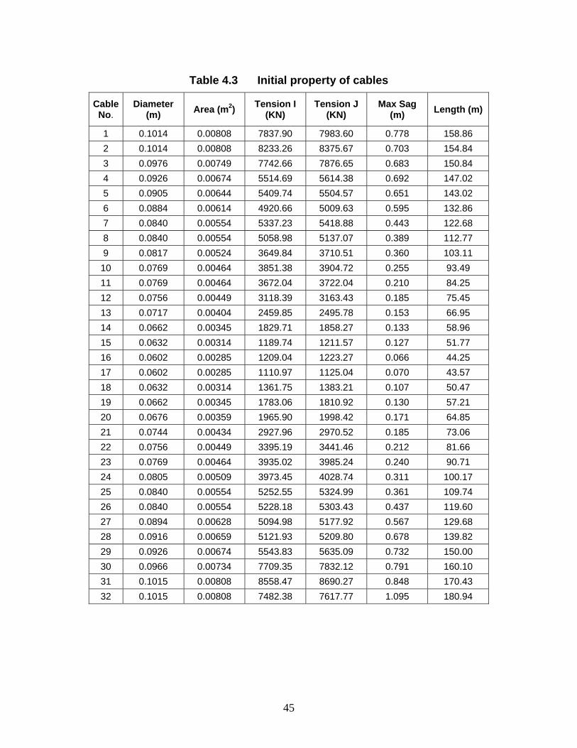
Table 4.3 Initial property of cables

Cable No.

Diameter (m) Area (m2) Tension I

(KN) Tension J

(KN) Max Sag

(m) Length (m)

1 0.1014 0.00808 7837.90 7983.60 0.778 158.86 2 0.1014 0.00808 8233.26 8375.67 0.703 154.84 3 0.0976 0.00749 7742.66 7876.65 0.683 150.84 4 0.0926 0.00674 5514.69 5614.38 0.692 147.02 5 0.0905 0.00644 5409.74 5504.57 0.651 143.02 6 0.0884 0.00614 4920.66 5009.63 0.595 132.86 7 0.0840 0.00554 5337.23 5418.88 0.443 122.68 8 0.0840 0.00554 5058.98 5137.07 0.389 112.77 9 0.0817 0.00524 3649.84 3710.51 0.360 103.11

10 0.0769 0.00464 3851.38 3904.72 0.255 93.49 11 0.0769 0.00464 3672.04 3722.04 0.210 84.25 12 0.0756 0.00449 3118.39 3163.43 0.185 75.45 13 0.0717 0.00404 2459.85 2495.78 0.153 66.95 14 0.0662 0.00345 1829.71 1858.27 0.133 58.96 15 0.0632 0.00314 1189.74 1211.57 0.127 51.77 16 0.0602 0.00285 1209.04 1223.27 0.066 44.25 17 0.0602 0.00285 1110.97 1125.04 0.070 43.57 18 0.0632 0.00314 1361.75 1383.21 0.107 50.47 19 0.0662 0.00345 1783.06 1810.92 0.130 57.21 20 0.0676 0.00359 1965.90 1998.42 0.171 64.85 21 0.0744 0.00434 2927.96 2970.52 0.185 73.06 22 0.0756 0.00449 3395.19 3441.46 0.212 81.66 23 0.0769 0.00464 3935.02 3985.24 0.240 90.71 24 0.0805 0.00509 3973.45 4028.74 0.311 100.17 25 0.0840 0.00554 5252.55 5324.99 0.361 109.74 26 0.0840 0.00554 5228.18 5303.43 0.437 119.60 27 0.0894 0.00628 5094.98 5177.92 0.567 129.68 28 0.0916 0.00659 5121.93 5209.80 0.678 139.82 29 0.0926 0.00674 5543.83 5635.09 0.732 150.00 30 0.0966 0.00734 7709.35 7832.12 0.791 160.10 31 0.1015 0.00808 8558.47 8690.27 0.848 170.43 32 0.1015 0.00808 7482.38 7617.77 1.095 180.94

45

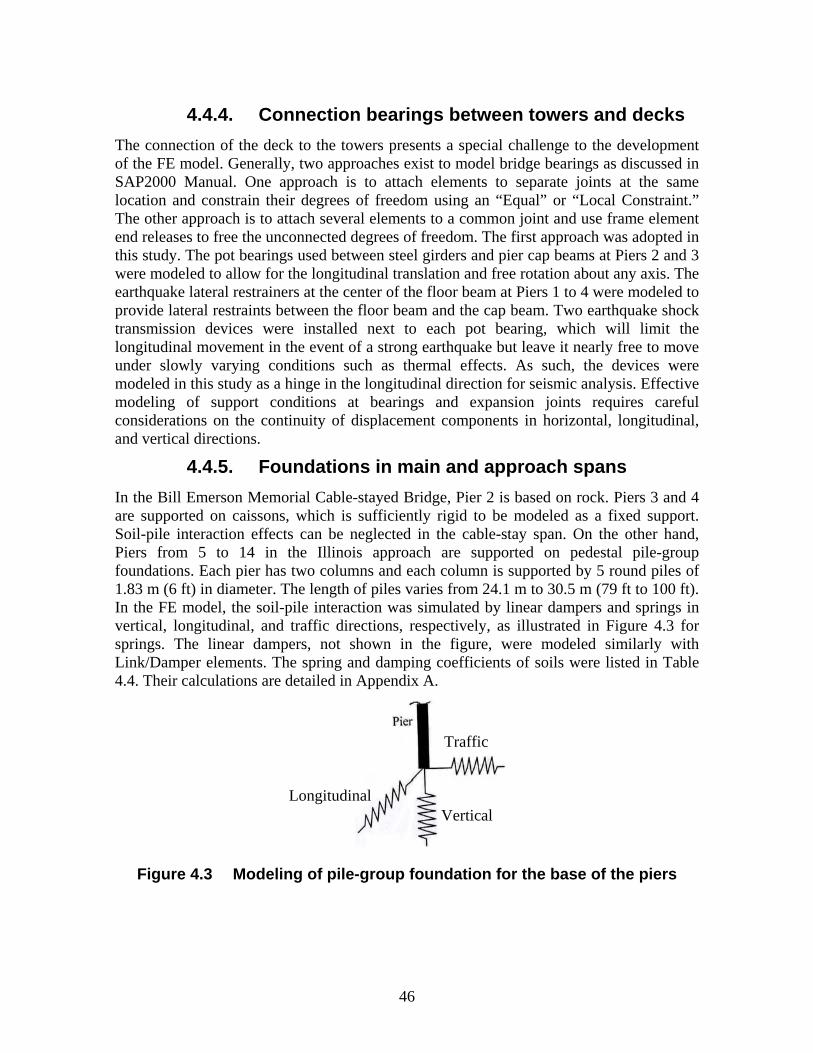
4.4.4. Connection bearings between towers and decks The connection of the deck to the towers presents a special challenge to the development of the FE model. Generally, two approaches exist to model bridge bearings as discussed in SAP2000 Manual. One approach is to attach elements to separate joints at the same location and constrain their degrees of freedom using an “Equal” or “Local Constraint.” The other approach is to attach several elements to a common joint and use frame element end releases to free the unconnected degrees of freedom. The first approach was adopted in this study. The pot bearings used between steel girders and pier cap beams at Piers 2 and 3 were modeled to allow for the longitudinal translation and free rotation about any axis. The earthquake lateral restrainers at the center of the floor beam at Piers 1 to 4 were modeled to provide lateral restraints between the floor beam and the cap beam. Two earthquake shock transmission devices were installed next to each pot bearing, which will limit the longitudinal movement in the event of a strong earthquake but leave it nearly free to move under slowly varying conditions such as thermal effects. As such, the devices were modeled in this study as a hinge in the longitudinal direction for seismic analysis. Effective modeling of support conditions at bearings and expansion joints requires careful considerations on the continuity of displacement components in horizontal, longitudinal, and vertical directions.

4.4.5. Foundations in main and approach spans In the Bill Emerson Memorial Cable-stayed Bridge, Pier 2 is based on rock. Piers 3 and 4 are supported on caissons, which is sufficiently rigid to be modeled as a fixed support. Soil-pile interaction effects can be neglected in the cable-stay span. On the other hand, Piers from 5 to 14 in the Illinois approach are supported on pedestal pile-group foundations. Each pier has two columns and each column is supported by 5 round piles of 1.83 m (6 ft) in diameter. The length of piles varies from 24.1 m to 30.5 m (79 ft to 100 ft). In the FE model, the soil-pile interaction was simulated by linear dampers and springs in vertical, longitudinal, and traffic directions, respectively, as illustrated in Figure 4.3 for springs. The linear dampers, not shown in the figure, were modeled similarly with Link/Damper elements. The spring and damping coefficients of soils were listed in Table 4.4. Their calculations are detailed in Appendix A.

Traffic

Longitudinal Vertical

Figure 4.3 Modeling of pile-group foundation for the base of the piers

46

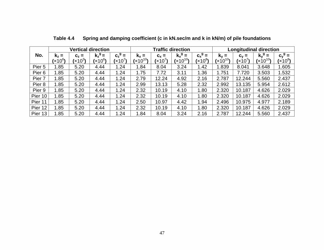
Table 4.4 Spring and damping coefficient (c in kN.sec/m and k in kN/m) of pile foundations

No. Vertical direction Traffic direction Longitudinal direction

kz = (×106)

cz = (×103)

g kz = (×106)

gcz = (×107)

kx = (×1010)

cx = (×107)

gkx = (×1010)

gcx = (×108)

ky = (×1010)

cy = (×107)

gky = (×1010)

gcy = (×108)

Pier 5 1.85 5.20 4.44 1.24 1.84 8.04 3.24 1.42 1.839 8.041 3.648 1.605 Pier 6 1.85 5.20 4.44 1.24 1.75 7.72 3.11 1.36 1.751 7.720 3.503 1.532 Pier 7 1.85 5.20 4.44 1.24 2.79 12.24 4.92 2.16 2.787 12.244 5.560 2.437 Pier 8 1.85 5.20 4.44 1.24 2.99 13.13 5.28 2.32 2.992 13.135 5.954 2.612 Pier 9 1.85 5.20 4.44 1.24 2.32 10.19 4.10 1.80 2.320 10.187 4.626 2.029 Pier 10 1.85 5.20 4.44 1.24 2.32 10.19 4.10 1.80 2.320 10.187 4.626 2.029 Pier 11 1.85 5.20 4.44 1.24 2.50 10.97 4.42 1.94 2.496 10.975 4.977 2.189 Pier 12 1.85 5.20 4.44 1.24 2.32 10.19 4.10 1.80 2.320 10.187 4.626 2.029 Pier 13 1.85 5.20 4.44 1.24 1.84 8.04 3.24 2.16 2.787 12.244 5.560 2.437

47

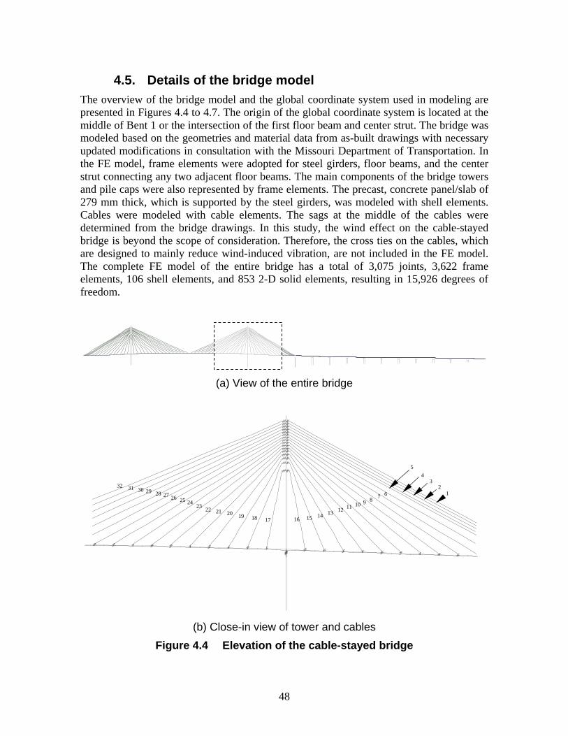
4.5. Details of the bridge model The overview of the bridge model and the global coordinate system used in modeling are presented in Figures 4.4 to 4.7. The origin of the global coordinate system is located at the middle of Bent 1 or the intersection of the first floor beam and center strut. The bridge was modeled based on the geometries and material data from as-built drawings with necessary updated modifications in consultation with the Missouri Department of Transportation. In the FE model, frame elements were adopted for steel girders, floor beams, and the center strut connecting any two adjacent floor beams. The main components of the bridge towers and pile caps were also represented by frame elements. The precast, concrete panel/slab of 279 mm thick, which is supported by the steel girders, was modeled with shell elements. Cables were modeled with cable elements. The sags at the middle of the cables were determined from the bridge drawings. In this study, the wind effect on the cable-stayed bridge is beyond the scope of consideration. Therefore, the cross ties on the cables, which are designed to mainly reduce wind-induced vibration, are not included in the FE model. The complete FE model of the entire bridge has a total of 3,075 joints, 3,622 frame elements, 106 shell elements, and 853 2-D solid elements, resulting in 15,926 degrees of freedom.

(a) View of the entire bridge

32 31 30 29 28 27 26 25 23

24 22 21 20 19 18 17 16 15 14 13 12 11 10 9 8 7 6 1

5 4

3 2

(b) Close-in view of tower and cables

Figure 4.4 Elevation of the cable-stayed bridge

48

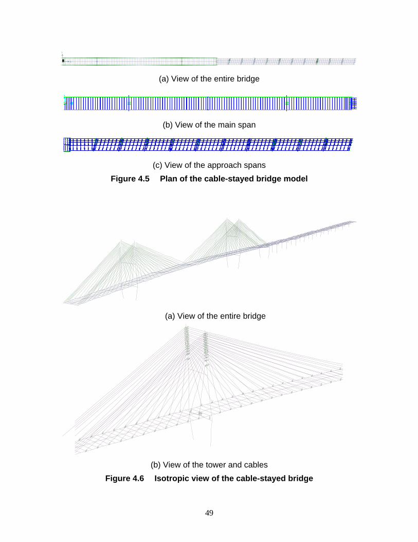
(a) View of the entire bridge

(b) View of the main span

(c) View of the approach spans

Figure 4.5 Plan of the cable-stayed bridge model

(a) View of the entire bridge

(b) View of the tower and cables

Figure 4.6 Isotropic view of the cable-stayed bridge

49

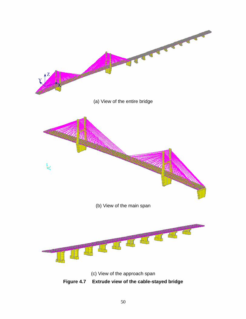
ZY

X

(a) View of the entire bridge

(b) View of the main span

(c) View of the approach span Figure 4.7 Extrude view of the cable-stayed bridge

50

4.6. Remarks A detailed 3-D FE model is established for the Bill Emerson Memorial Cable-stayed Bridges. The model has explicitly simulated all primary members of the complex structure. It will be refined and validated with field measured data in Section 5. Following is a brief summary of main observations and comments on the model:

1. In order to model the actual length and configuration of each cable as specified in the as-built drawings, one rigid link element is introduced in the FE model at each end of the cable. Long cables are more flexible than short cables. They all significantly influence the stiffness of the bridge system.

2. The sagging of cables should be taken into account in the modeling of the cable-stayed bridge because it usually plays an important role in the dynamic response of the large-scale structure.

3 Boundary conditions in actual situations are usually complex; at the same time, they have significant effects on the dynamic behavior of the bridge. As such, extra attention must be paid to the modeling process of bearings at each pier both in the main span and in the approach part of the bridge.

51

5. Eigensolution and Model Verification of the Cable-stayed Bridge

5.1. General Cable-stayed bridges, due to their large scale and high flexibility, usually have a long fundamental period, which distinguishes themselves from most of other structures. As a result, they are sensitive to ambient motions such as traffic and tremor induced vibration. In this section, the natural frequencies and mode shapes of the cable-stayed bridge are evaluated using the FE model developed in the preceding section. They are then compared with measured data to validate the FE model.

5.2. Modal analysis Modal analysis in structural dynamics is aimed to determine the natural frequencies and mode shapes of a structure and evaluate its responses under dynamic loading. In most cases, only a small number of lowest vibration modes dominate the responses of an engineering structure such as cable-stayed bridge.

5.2.1. Classical modal analysis theory The equation of motion of a linear multiple degree of freedom (MDF) system without damping can be written as:

[M ]{ (U t&& )}+ =[K ]{ (U t)} {P(t)} (5.1)

in which [M ] and [K ] are the mass and stiffness matrices of the structural system, { (U t)}is the displacement vector as a function of time t, and {P t( )}is the external load vector.

The displacement vector {U t( )} of an MDF system can be expanded into a summation of modal contributions, i.e.,

N{U t( )} = =∑{φr r}q (t) [Φ]{q(t)} (5.2)

r=1

where N is the number of degrees of freedom, {φr}is the rth mode vector, [Φ] is a collection of all mode vectors, q tr ( ) is the rth modal displacement, and {q t( )}is a generalized displacement vector or a collection of modal displacement. By using Eq. (5.2), the coupled equation (5.1) in {U t( )}can be transformed to a set of uncoupled equations with the unknown modal displacement qn (t) after modal orthogonality conditions have been introduced (Chopra, 2006). That is,

m q&&n n ( )t + kn nq ( )t = pn ( )t (5.3)

in which m M{ }Tn n= φ [ ]{ }φn and k K{ }T

n n= φ [ ]{ }φn are the nth modal mass and stiffness, pn n( )t P= {φ }T { ( )t } is a nth modal force. Eq. (5.3) represents a generalized single degree

of freedom (SDF) system. The natural frequency ωn of the SDF system can be evaluated by:

52

kω nn = (5.4)

mn

Similarly, when damping is present, the nth modal equation of motion can be derived as

mnq&&n ( )t + cn nq& + =kn nq t( ) p tn ( ) (5.5)

where c is th thn e damping coefficient of the n mode of vibration. Eq. (5.5) indicates that

the nth modal displacement q tn ( ) depends on its corresponding natural frequencyωn ,

damping ratio c mn n/ 2 kn , and the frequency content of external excitation. After the modal displacement q (t) has been determined, the contribution of the nth

n mode to the displacement {U t( )} can be evaluated by Eq. (5.2).

5.2.2. Modal analysis of Bill Emerson Memorial cable-stayed bridge

The natural frequencies and mode vectors of the cable-stayed bridge were determined by an eigensolution method. For time-history analyses, the so-called Ritz-vector method is used. This is because Ritz-vectors can provide a better basis than eigenvectors do when used for response-spectrum or time-history analysis (Wilson, 1982). The Ritz vectors are generated by taking into account the spatial distribution of the dynamic loading, whereas the direct use of natural mode shapes neglects this very important information.

How many modes of vibration must be included in analysis is a practical question. In building design, a rule of thumb is to have accumulated modal participating mass factors in all directions of over 90%. For complex 3-D cable-stayed bridge structures, it is extremely difficult to achieve that level of mass participation in all directions. In this study, an effort is made to include an accumulated modal participating mass factor of over 70% in every direction. To this endeavor, a total of 4000 modes are specified in the initial analysis of the cable-stayed bridge. The relationship between natural frequency and mode number is depicted in Figure 5.1. It was observed that the natural frequencies of the bridge up to 45.54 Hz were covered. The model was calibrated by slightly increasing the mass density of concrete so that the first several natural frequencies can match the experimental frequencies obtained from the measured responses. This modification mainly represents the uncertainty of material density and geometry and the effects of non-structural components such as bracings, railing supports, and other permanent attachments.

53

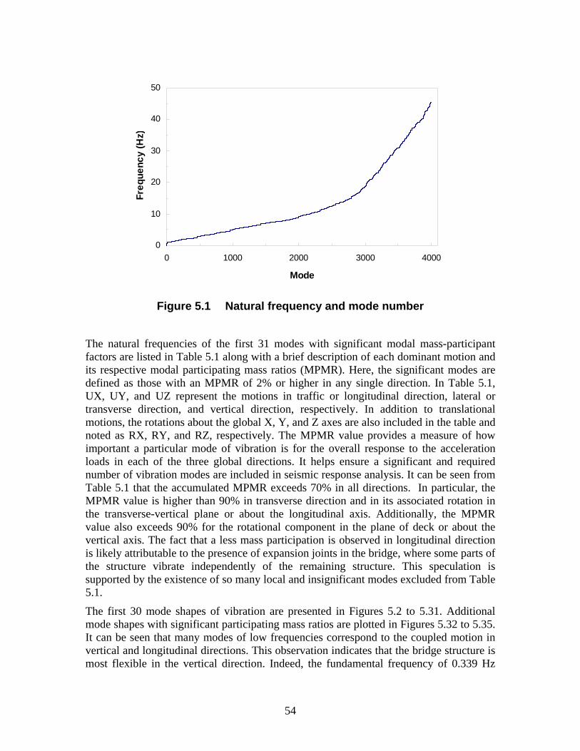
0

10

20

30

40

50

0 1000 2000 3000 4000

Mode

Freq

uenc

y (H

z)

Figure 5.1 Natural frequency and mode number

The natural frequencies of the first 31 modes with significant modal mass-participant factors are listed in Table 5.1 along with a brief description of each dominant motion and its respective modal participating mass ratios (MPMR). Here, the significant modes are defined as those with an MPMR of 2% or higher in any single direction. In Table 5.1, UX, UY, and UZ represent the motions in traffic or longitudinal direction, lateral or transverse direction, and vertical direction, respectively. In addition to translational motions, the rotations about the global X, Y, and Z axes are also included in the table and noted as RX, RY, and RZ, respectively. The MPMR value provides a measure of how important a particular mode of vibration is for the overall response to the acceleration loads in each of the three global directions. It helps ensure a significant and required number of vibration modes are included in seismic response analysis. It can be seen from Table 5.1 that the accumulated MPMR exceeds 70% in all directions. In particular, the MPMR value is higher than 90% in transverse direction and in its associated rotation in the transverse-vertical plane or about the longitudinal axis. Additionally, the MPMR value also exceeds 90% for the rotational component in the plane of deck or about the vertical axis. The fact that a less mass participation is observed in longitudinal direction is likely attributable to the presence of expansion joints in the bridge, where some parts of the structure vibrate independently of the remaining structure. This speculation is supported by the existence of so many local and insignificant modes excluded from Table 5.1.

The first 30 mode shapes of vibration are presented in Figures 5.2 to 5.31. Additional mode shapes with significant participating mass ratios are plotted in Figures 5.32 to 5.35. It can be seen that many modes of low frequencies correspond to the coupled motion in vertical and longitudinal directions. This observation indicates that the bridge structure is most flexible in the vertical direction. Indeed, the fundamental frequency of 0.339 Hz

54

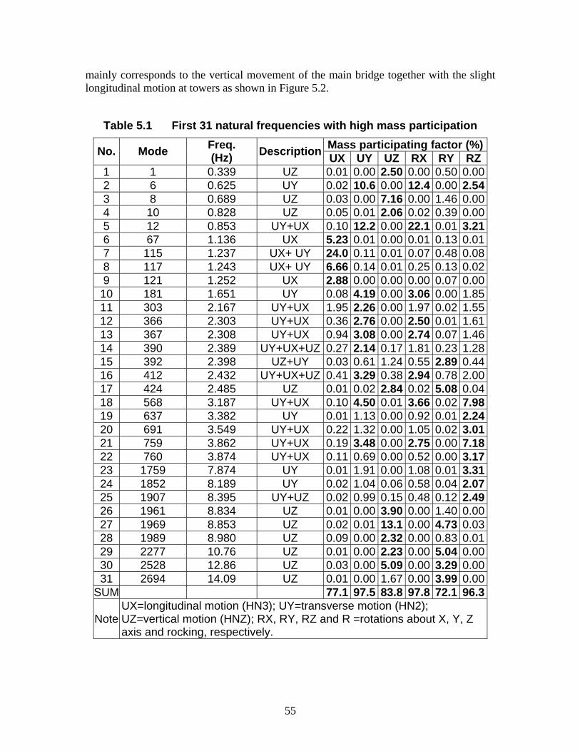
55

mainly corresponds to the vertical movement of the main bridge together with the slight longitudinal motion at towers as shown in Figure 5.2.

Table 5.1 First 31 natural frequencies with high mass participation

No. Mode Freq. (Hz) Description Mass participating factor (%)

UX UY UZ RX RY RZ1 1 0.339 UZ 0.01 0.00 2.50 0.00 0.50 0.002 6 0.625 UY 0.02 10.6 0.00 12.4 0.00 2.543 8 0.689 UZ 0.03 0.00 7.16 0.00 1.46 0.004 10 0.828 UZ 0.05 0.01 2.06 0.02 0.39 0.005 12 0.853 UY+UX 0.10 12.2 0.00 22.1 0.01 3.216 67 1.136 UX 5.23 0.01 0.00 0.01 0.13 0.017 115 1.237 UX+ UY 24.0 0.11 0.01 0.07 0.48 0.088 117 1.243 UX+ UY 6.66 0.14 0.01 0.25 0.13 0.029 121 1.252 UX 2.88 0.00 0.00 0.00 0.07 0.0010 181 1.651 UY 0.08 4.19 0.00 3.06 0.00 1.8511 303 2.167 UY+UX 1.95 2.26 0.00 1.97 0.02 1.5512 366 2.303 UY+UX 0.36 2.76 0.00 2.50 0.01 1.6113 367 2.308 UY+UX 0.94 3.08 0.00 2.74 0.07 1.4614 390 2.389 UY+UX+UZ 0.27 2.14 0.17 1.81 0.23 1.2815 392 2.398 UZ+UY 0.03 0.61 1.24 0.55 2.89 0.4416 412 2.432 UY+UX+UZ 0.41 3.29 0.38 2.94 0.78 2.0017 424 2.485 UZ 0.01 0.02 2.84 0.02 5.08 0.0418 568 3.187 UY+UX 0.10 4.50 0.01 3.66 0.02 7.9819 637 3.382 UY 0.01 1.13 0.00 0.92 0.01 2.2420 691 3.549 UY+UX 0.22 1.32 0.00 1.05 0.02 3.0121 759 3.862 UY+UX 0.19 3.48 0.00 2.75 0.00 7.1822 760 3.874 UY+UX 0.11 0.69 0.00 0.52 0.00 3.1723 1759 7.874 UY 0.01 1.91 0.00 1.08 0.01 3.3124 1852 8.189 UY 0.02 1.04 0.06 0.58 0.04 2.0725 1907 8.395 UY+UZ 0.02 0.99 0.15 0.48 0.12 2.4926 1961 8.834 UZ 0.01 0.00 3.90 0.00 1.40 0.0027 1969 8.853 UZ 0.02 0.01 13.1 0.00 4.73 0.0328 1989 8.980 UZ 0.09 0.00 2.32 0.00 0.83 0.0129 2277 10.76 UZ 0.01 0.00 2.23 0.00 5.04 0.0030 2528 12.86 UZ 0.03 0.00 5.09 0.00 3.29 0.0031 2694 14.09 UZ 0.01 0.00 1.67 0.00 3.99 0.00

SUM 77.1 97.5 83.8 97.8 72.1 96.3UX=longitudinal motion (HN3); UY=transverse motion (HN2);

Note UZ=vertical motion (HNZ); RX, RY, RZ and R =rotations about X, Y, Z axis and rocking, respectively.

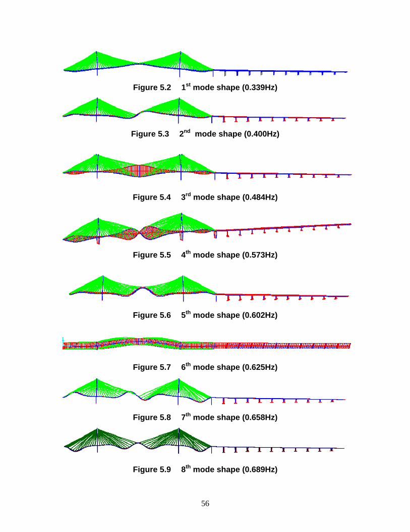
stFigure 5.2 1 mode shape (0.339Hz)

ndFigure 5.3 2 mode shape (0.400Hz)

rdFigure 5.4 3 mode shape (0.484Hz)

thFigure 5.5 4 mode shape (0.573Hz)

thFigure 5.6 5 mode shape (0.602Hz)

th mode shape (0.625Hz) Figure 5.7 6

th mode shape (0.658Hz) Figure 5.8 7

thFigure 5.9 8 mode shape (0.689Hz)

56

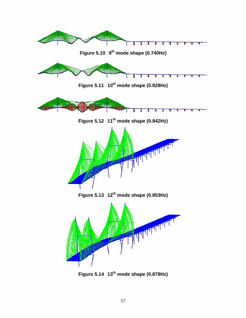
thFigure 5.10 9 mode shape (0.740Hz)

thFigure 5.11 10 mode shape (0.828Hz)

thFigure 5.12 11 mode shape (0.842Hz)

thFigure 5.13 12 mode shape (0.853Hz)

thFigure 5.14 13 mode shape (0.878Hz)

57

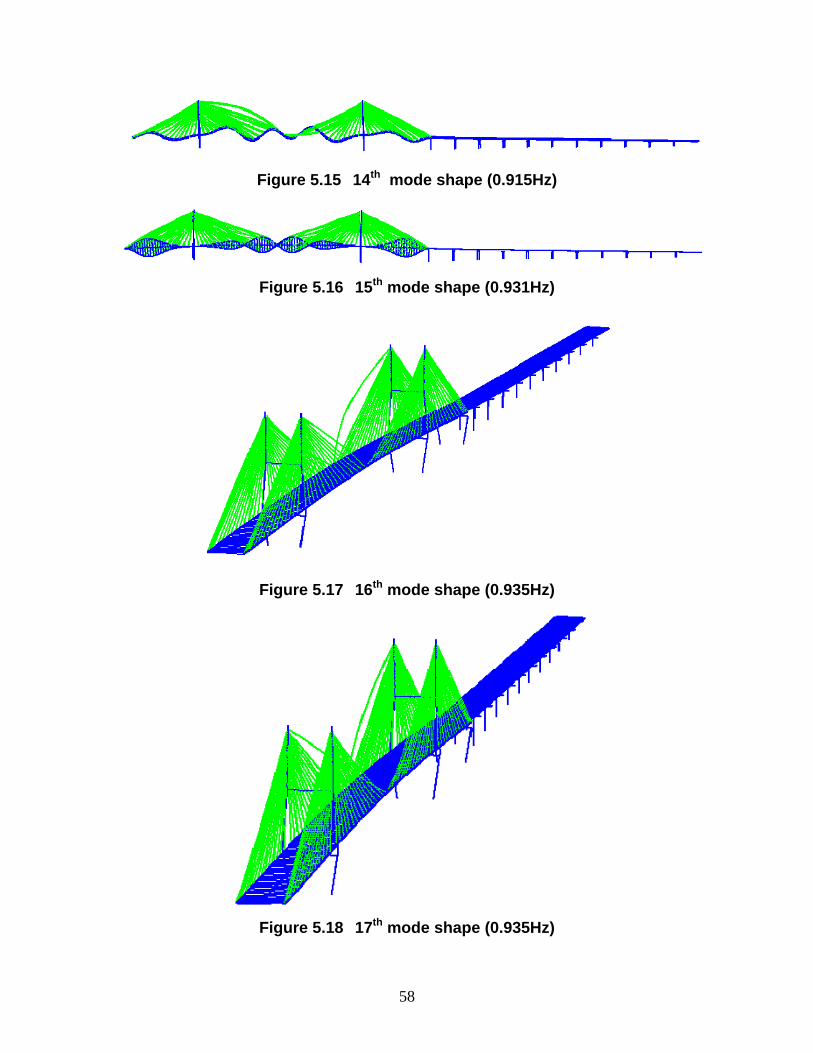
thFigure 5.15 14 mode shape (0.915Hz)

thFigure 5.16 15 mode shape (0.931Hz)

thFigure 5.17 16 mode shape (0.935Hz)

thFigure 5.18 17 mode shape (0.935Hz)

58

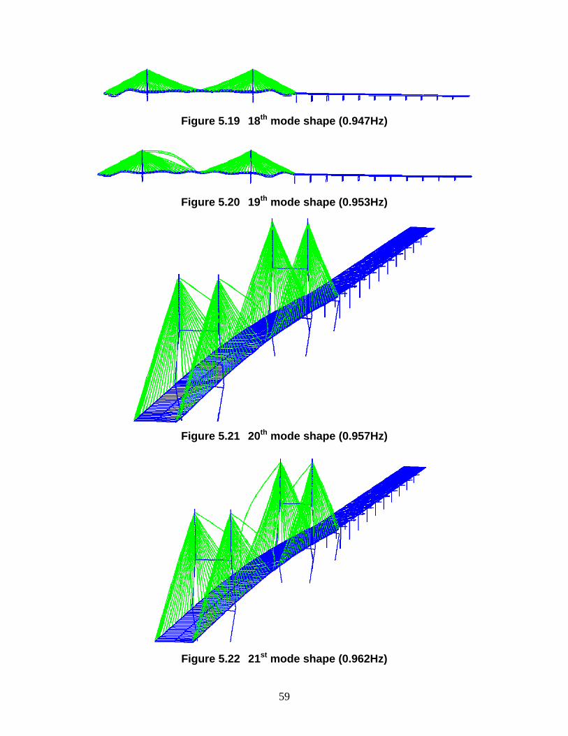
thFigure 5.19 18 mode shape (0.947Hz)

thFigure 5.20 19 mode shape (0.953Hz)

thFigure 5.21 20 mode shape (0.957Hz)

stFigure 5.22 21 mode shape (0.962Hz)

59

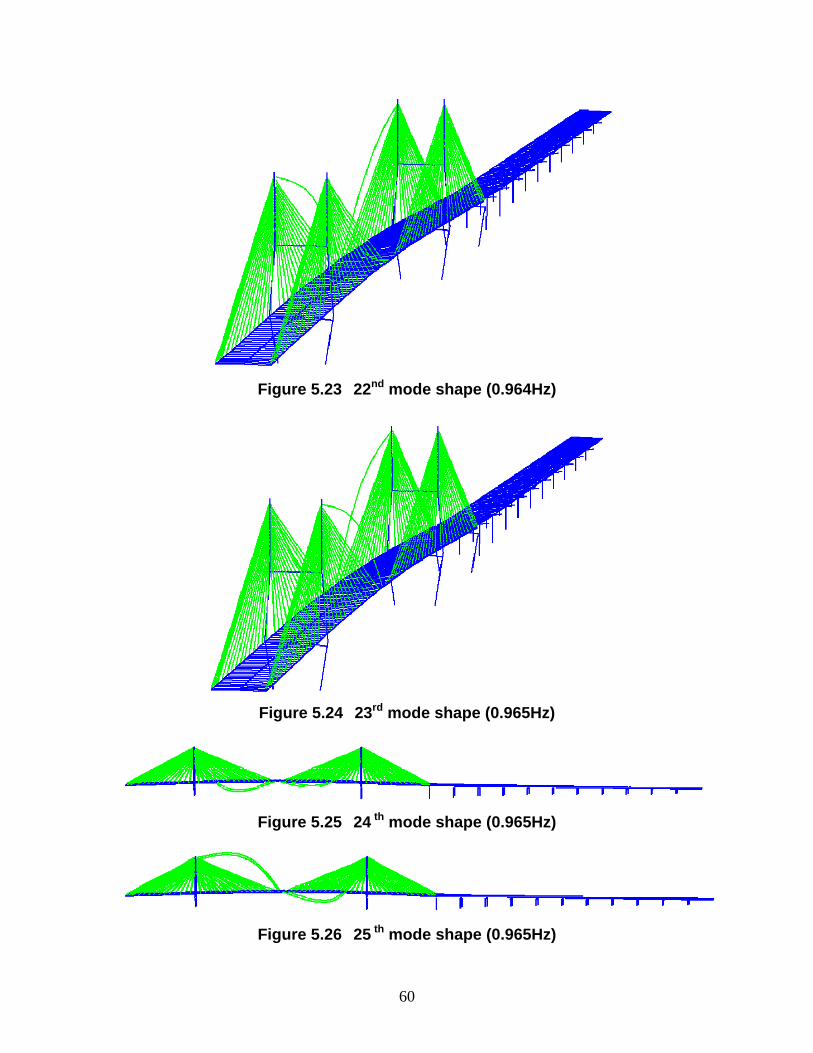
ndFigure 5.23 22 mode shape (0.964Hz)

rd mode shape (0.965Hz) Figure 5.24 23

thFigure 5.25 24 mode shape (0.965Hz)

thFigure 5.26 25 mode shape (0.965Hz)

60

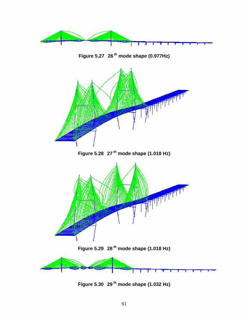
th mode shape (0.977Hz) Figure 5.27 26

thFigure 5.28 27 mode shape (1.018 Hz)

thFigure 5.29 28 mode shape (1.018 Hz)

thFigure 5.30 29 mode shape (1.032 Hz)

61

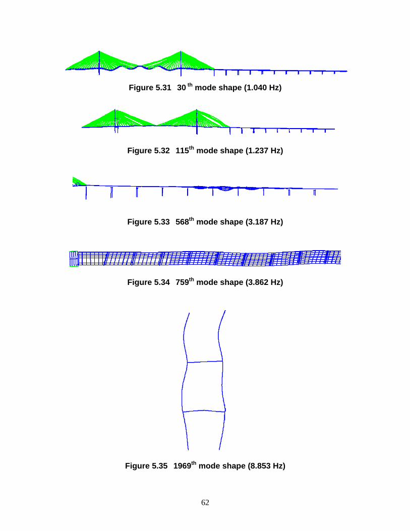
th mode shape (1.040 Hz) Figure 5.31 30

thFigure 5.32 115 mode shape (1.237 Hz)

thFigure 5.33 568 mode shape (3.187 Hz)

thFigure 5.34 759 mode shape (3.862 Hz)

thFigure 5.35 1969 mode shape (8.853 Hz)

62

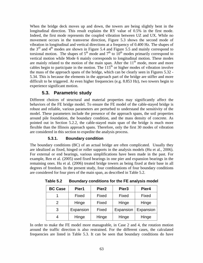
When the bridge deck moves up and down, the towers are being slightly bent in the longitudinal direction. This result explains the RY value of 0.5% in the first mode. Indeed, the first mode represents the coupled vibration between UZ and UX. While no movement occurs in the transverse direction, Figure 5.3 shows the second mode of vibration in longitudinal and vertical directions at a frequency of 0.400 Hz. The shapes of the 3rd and 4th modes are shown in Figure 5.4 and Figure 5.5 and mainly correspond to torsional motion. The shapes of 5th mode and 7th to 10th modes primarily correspond to vertical motion while Mode 6 mainly corresponds to longitudinal motion. These modes are mainly related to the motion of the main span. After the 11th mode, more and more cables begin to participate in the motion. The 115th or higher modes of vibration involve the mass of the approach spans of the bridge, which can be clearly seen in Figures 5.32 -5.34. This is because the elements in the approach part of the bridge are stiffer and more difficult to be triggered. At even higher frequencies (e.g. 8.853 Hz), two towers begin to experience significant motion.

5.3. Parametric study Different choices of structural and material properties may significantly affect the behaviors of the FE bridge model. To ensure the FE model of the cable-stayed bridge is robust and reliable, various parameters are perturbed to understand the sensitivity of the model. These parameters include the presence of the approach spans, the soil properties around pile foundation, the boundary condition, and the mass density of concrete. As pointed out in Section 5.2.2, the cable-stayed main span of the bridge is much more flexible than the Illinois approach spans. Therefore, only the first 30 modes of vibration are considered in this section to expedite the analysis process.

5.3.1. Boundary condition The boundary conditions (BC) of an actual bridge are often complicated. Usually they are idealized as fixed, hinged or roller supports in the analysis models (Hu et al., 2006). For external or end bearings, various simplifications have been made in the past. For example, Ren et al. (2005) used fixed bearings in one pier and expansion bearings in the remaining ones. Hu et al. (2006) treated bridge towers as being fixed at their base in all degrees of freedom. In the present study, four combinations of four boundary conditions are considered for four piers of the main span, as described in Table 5.2.

Table 5.2 Boundary conditions for the FE analysis model

BC Case Pier1 Pier2 Pier3 Pier41 Fixed Fixed Fixed Fixed

2 Hinge Fixed Hinge Hinge

3 Expansion Fixed Expansion Expansion

4 Hinge Hinge Hinge Hinge

In order to make the FE model more manageable, in Case 2 and 4, the rotation motion around the traffic direction is also restrained. For the different cases, the calculated frequencies are listed in Table 5.3. It can be seen that boundary conditions do have

63

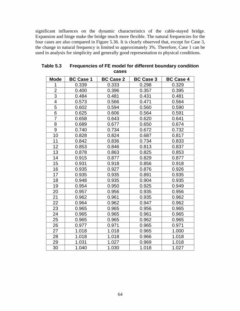
significant influences on the dynamic characteristics of the cable-stayed bridge. Expansion and hinge make the bridge much more flexible. The natural frequencies for the four cases are also compared in Figure 5.36. It is clearly observed that, except for Case 3, the change in natural frequency is limited to approximately 3%. Therefore, Case 1 can be used in analysis for simplicity and generally good representation to physical conditions.

Table 5.3 Frequencies of FE model for different boundary condition

cases Mode BC Case 1 BC Case 2 BC Case 3 BC Case 4

1 0.339 0.333 0.298 0.329 2 0.400 0.396 0.357 0.395 3 0.484 0.481 0.431 0.481 4 0.573 0.566 0.471 0.564 5 0.602 0.594 0.560 0.590 6 0.625 0.606 0.564 0.591 7 0.658 0.643 0.620 0.641 8 0.689 0.677 0.650 0.674 9 0.740 0.734 0.672 0.732

10 0.828 0.824 0.687 0.817 11 0.842 0.836 0.734 0.833 12 0.853 0.846 0.813 0.837 13 0.878 0.863 0.825 0.853 14 0.915 0.877 0.829 0.877 15 0.931 0.918 0.856 0.918 16 0.935 0.927 0.876 0.926 17 0.935 0.935 0.891 0.935 18 0.948 0.935 0.904 0.935 19 0.954 0.950 0.925 0.949 20 0.957 0.956 0.935 0.956 21 0.962 0.961 0.935 0.962 22 0.964 0.962 0.947 0.962 23 0.965 0.965 0.956 0.965 24 0.965 0.965 0.961 0.965 25 0.965 0.965 0.962 0.965 26 0.977 0.971 0.965 0.971 27 1.018 1.018 0.965 1.000 28 1.018 1.018 0.966 1.018 29 1.031 1.027 0.969 1.018 30 1.040 1.030 1.018 1.027

64

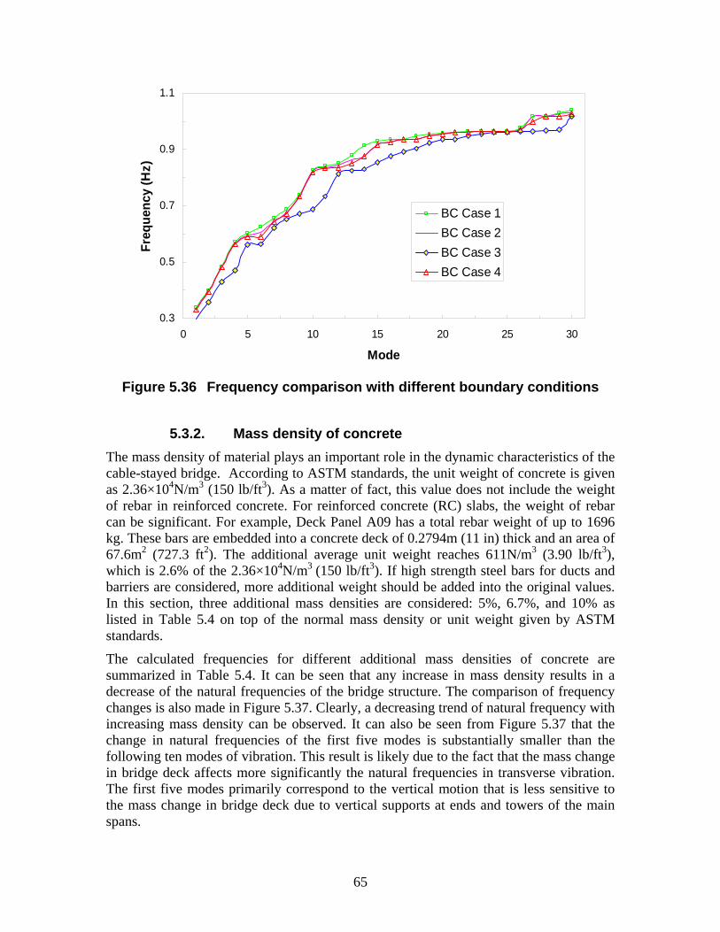
0.3

0.5

0.7

0.9

1.1

0 5 10 15 20 25 30

Mode

Freq

uenc

y (H

z)

BC Case 1BC Case 2BC Case 3BC Case 4

Figure 5.36 Frequency comparison with different boundary conditions

5.3.2. Mass density of concrete The mass density of material plays an important role in the dynamic characteristics of the cable-stayed bridge. According to ASTM standards, the unit weight of concrete is given as 2.36×104N/m3 3 (150 lb/ft ). As a matter of fact, this value does not include the weight of rebar in reinforced concrete. For reinforced concrete (RC) slabs, the weight of rebar can be significant. For example, Deck Panel A09 has a total rebar weight of up to 1696 kg. These bars are embedded into a concrete deck of 0.2794m (11 in) thick and an area of 67.6m2 2 (727.3 ft ). The additional average unit weight reaches 611N/m3 3 (3.90 lb/ft ), which is 2.6% of the 2.36×104N/m3 (150 lb/ft3). If high strength steel bars for ducts and barriers are considered, more additional weight should be added into the original values. In this section, three additional mass densities are considered: 5%, 6.7%, and 10% as listed in Table 5.4 on top of the normal mass density or unit weight given by ASTM standards.

The calculated frequencies for different additional mass densities of concrete are summarized in Table 5.4. It can be seen that any increase in mass density results in a decrease of the natural frequencies of the bridge structure. The comparison of frequency changes is also made in Figure 5.37. Clearly, a decreasing trend of natural frequency with increasing mass density can be observed. It can also be seen from Figure 5.37 that the change in natural frequencies of the first five modes is substantially smaller than the following ten modes of vibration. This result is likely due to the fact that the mass change in bridge deck affects more significantly the natural frequencies in transverse vibration. The first five modes primarily correspond to the vertical motion that is less sensitive to the mass change in bridge deck due to vertical supports at ends and towers of the main spans.

65

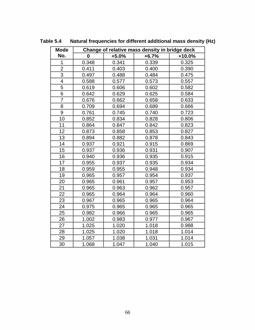
Table 5.4 Natural frequencies for different additional mass density (Hz)

Mode No.

Change of relative mass density in bridge deck 0 +5.0% +6.7% +10.0%

1 0.348 0.341 0.339 0.325 2 0.411 0.403 0.400 0.390 3 0.497 0.488 0.484 0.475 4 0.588 0.577 0.573 0.557 5 0.619 0.606 0.602 0.582 6 0.642 0.629 0.625 0.584 7 0.676 0.662 0.658 0.633 8 0.709 0.694 0.689 0.666 9 0.761 0.745 0.740 0.723

10 0.852 0.834 0.828 0.806 11 0.864 0.847 0.842 0.823 12 0.873 0.858 0.853 0.827 13 0.894 0.882 0.878 0.843 14 0.937 0.921 0.915 0.869 15 0.937 0.936 0.931 0.907 16 0.940 0.936 0.935 0.915 17 0.955 0.937 0.935 0.934 18 0.959 0.955 0.948 0.934 19 0.965 0.957 0.954 0.937 20 0.965 0.961 0.957 0.953 21 0.965 0.963 0.962 0.957 22 0.965 0.964 0.964 0.960 23 0.967 0.965 0.965 0.964 24 0.975 0.965 0.965 0.965 25 0.982 0.966 0.965 0.965 26 1.002 0.983 0.977 0.967 27 1.025 1.020 1.018 0.988 28 1.025 1.020 1.018 1.014 29 1.057 1.038 1.031 1.014 30 1.068 1.047 1.040 1.015

66

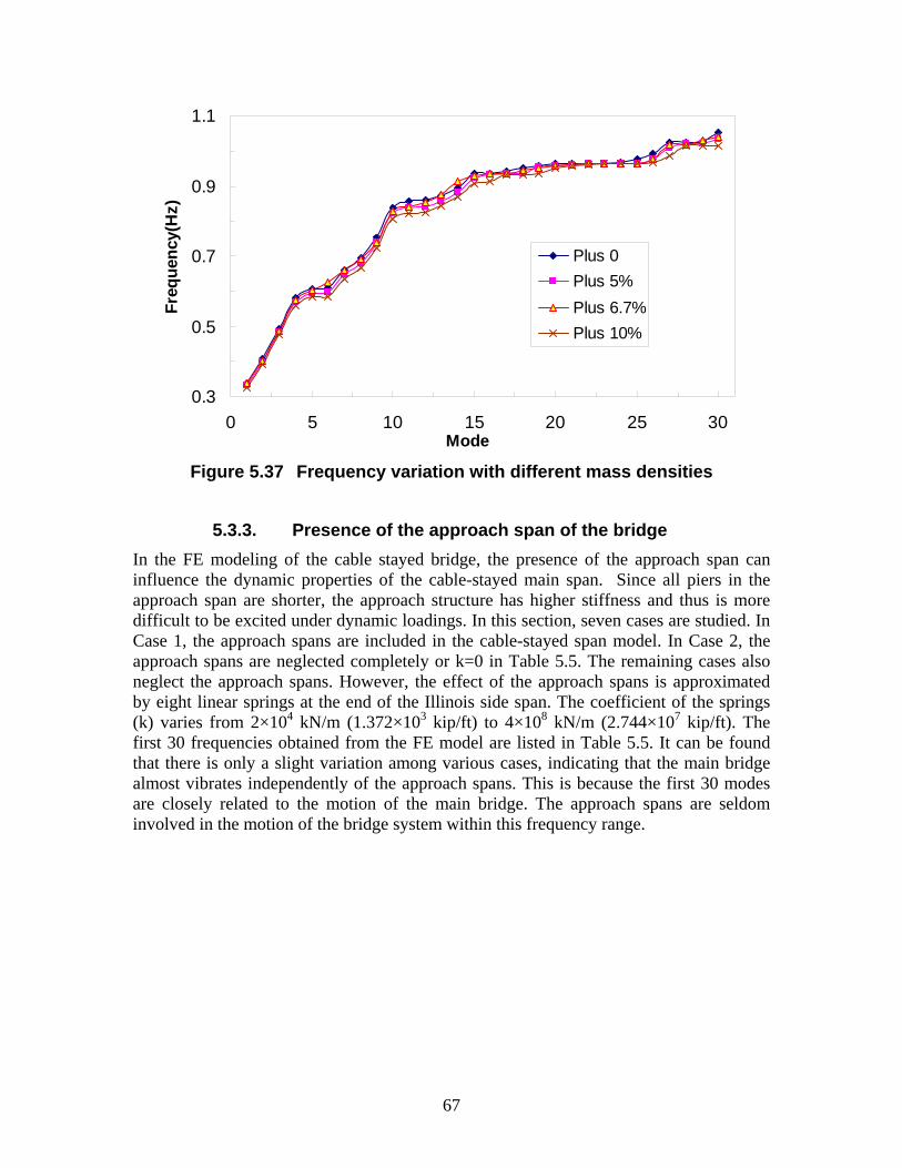
0.3

0.5

0.7

0.9

1.1

0 5 10 15 20 25 30Mode

Freq

uenc

y(H

z)

Plus 0Plus 5%Plus 6.7%Plus 10%

Figure 5.37 Frequency variation with different mass densities

5.3.3. Presence of the approach span of the bridge In the FE modeling of the cable stayed bridge, the presence of the approach span can influence the dynamic properties of the cable-stayed main span. Since all piers in the approach span are shorter, the approach structure has higher stiffness and thus is more difficult to be excited under dynamic loadings. In this section, seven cases are studied. In Case 1, the approach spans are included in the cable-stayed span model. In Case 2, the approach spans are neglected completely or k=0 in Table 5.5. The remaining cases also neglect the approach spans. However, the effect of the approach spans is approximated by eight linear springs at the end of the Illinois side span. The coefficient of the springs (k) varies from 2×104 kN/m (1.372×103 kip/ft) to 4×108 kN/m (2.744×107 kip/ft). The first 30 frequencies obtained from the FE model are listed in Table 5.5. It can be found that there is only a slight variation among various cases, indicating that the main bridge almost vibrates independently of the approach spans. This is because the first 30 modes are closely related to the motion of the main bridge. The approach spans are seldom involved in the motion of the bridge system within this frequency range.

67

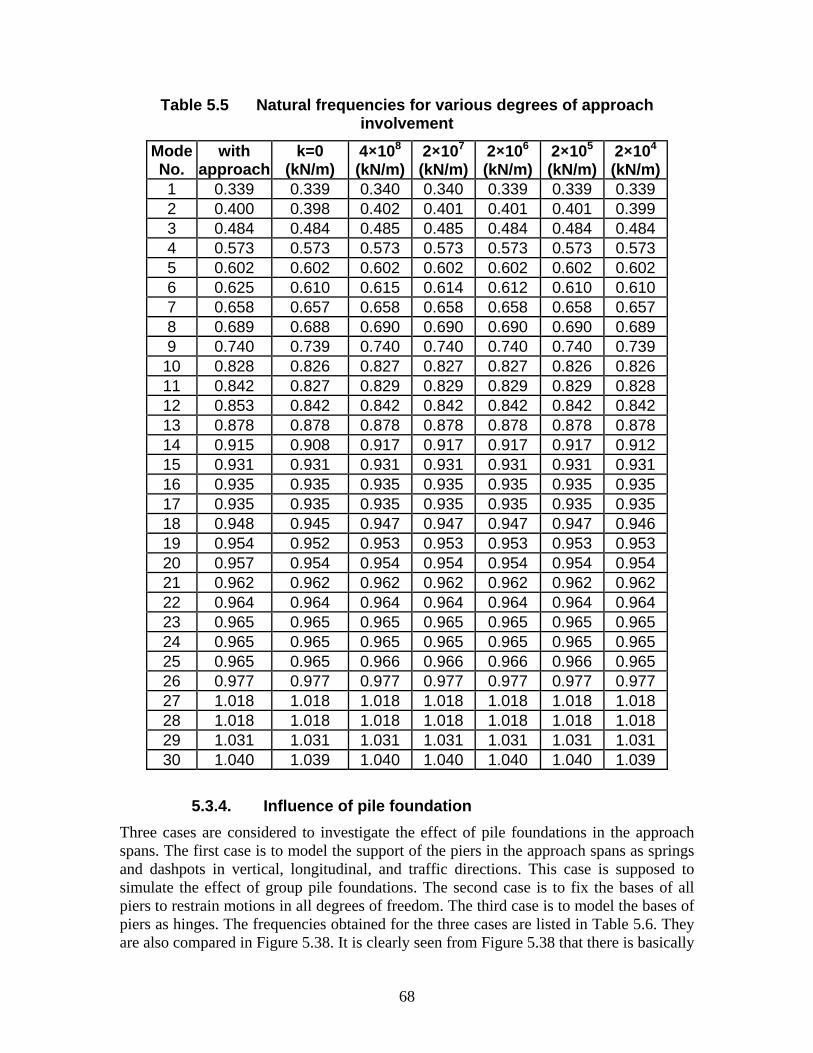
Table 5.5 Natural frequencies for various degrees of approach involvement

Mode No.

with approach

k=0 (kN/m)

84×10(kN/m)

72×10 (kN/m)

62×10 (kN/m)

52×10 (kN/m)

42×10 (kN/m)

1 0.339 0.339 0.340 0.340 0.339 0.339 0.339 2 0.400 0.398 0.402 0.401 0.401 0.401 0.399 3 0.484 0.484 0.485 0.485 0.484 0.484 0.484 4 0.573 0.573 0.573 0.573 0.573 0.573 0.573 5 0.602 0.602 0.602 0.602 0.602 0.602 0.602 6 0.625 0.610 0.615 0.614 0.612 0.610 0.610 7 0.658 0.657 0.658 0.658 0.658 0.658 0.657 8 0.689 0.688 0.690 0.690 0.690 0.690 0.689 9 0.740 0.739 0.740 0.740 0.740 0.740 0.739

10 0.828 0.826 0.827 0.827 0.827 0.826 0.826 11 0.842 0.827 0.829 0.829 0.829 0.829 0.828 12 0.853 0.842 0.842 0.842 0.842 0.842 0.842 13 0.878 0.878 0.878 0.878 0.878 0.878 0.878 14 0.915 0.908 0.917 0.917 0.917 0.917 0.912 15 0.931 0.931 0.931 0.931 0.931 0.931 0.931 16 0.935 0.935 0.935 0.935 0.935 0.935 0.935 17 0.935 0.935 0.935 0.935 0.935 0.935 0.935 18 0.948 0.945 0.947 0.947 0.947 0.947 0.946 19 0.954 0.952 0.953 0.953 0.953 0.953 0.953 20 0.957 0.954 0.954 0.954 0.954 0.954 0.954 21 0.962 0.962 0.962 0.962 0.962 0.962 0.962 22 0.964 0.964 0.964 0.964 0.964 0.964 0.964 23 0.965 0.965 0.965 0.965 0.965 0.965 0.965 24 0.965 0.965 0.965 0.965 0.965 0.965 0.965 25 0.965 0.965 0.966 0.966 0.966 0.966 0.965 26 0.977 0.977 0.977 0.977 0.977 0.977 0.977 27 1.018 1.018 1.018 1.018 1.018 1.018 1.018 28 1.018 1.018 1.018 1.018 1.018 1.018 1.018 29 1.031 1.031 1.031 1.031 1.031 1.031 1.031 30 1.040 1.039 1.040 1.040 1.040 1.040 1.039

5.3.4. Influence of pile foundation Three cases are considered to investigate the effect of pile foundations in the approach spans. The first case is to model the support of the piers in the approach spans as springs and dashpots in vertical, longitudinal, and traffic directions. This case is supposed to simulate the effect of group pile foundations. The second case is to fix the bases of all piers to restrain motions in all degrees of freedom. The third case is to model the bases of piers as hinges. The frequencies obtained for the three cases are listed in Table 5.6. They are also compared in Figure 5.38. It is clearly seen from Figure 5.38 that there is basically

68

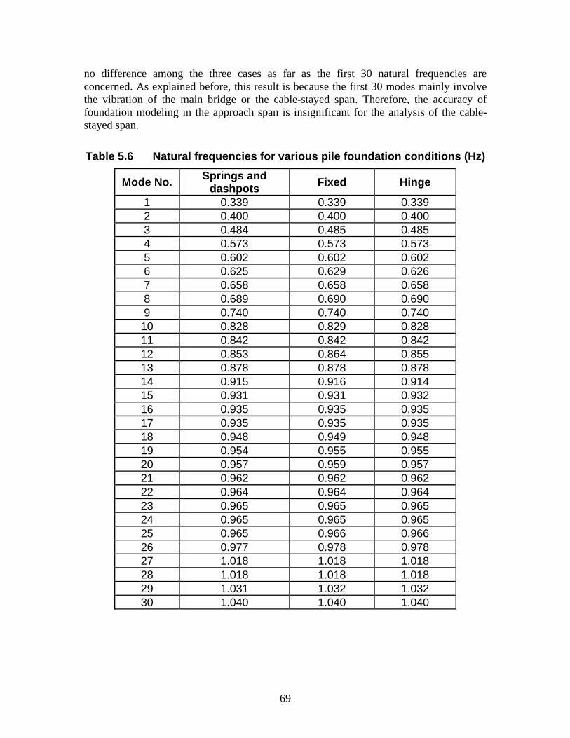
no difference among the three cases as far as the first 30 natural frequencies are concerned. As explained before, this result is because the first 30 modes mainly involve the vibration of the main bridge or the cable-stayed span. Therefore, the accuracy of foundation modeling in the approach span is insignificant for the analysis of the cable-stayed span.

Table 5.6 Natural frequencies for various pile foundation conditions (Hz)

Mode No. Springs and dashpots Fixed Hinge

1 0.339 0.339 0.339 2 0.400 0.400 0.400 3 0.484 0.485 0.485 4 0.573 0.573 0.573 5 0.602 0.602 0.602 6 0.625 0.629 0.626 7 0.658 0.658 0.658 8 0.689 0.690 0.690 9 0.740 0.740 0.740

10 0.828 0.829 0.828 11 0.842 0.842 0.842 12 0.853 0.864 0.855 13 0.878 0.878 0.878 14 0.915 0.916 0.914 15 0.931 0.931 0.932 16 0.935 0.935 0.935 17 0.935 0.935 0.935 18 0.948 0.949 0.948 19 0.954 0.955 0.955 20 0.957 0.959 0.957 21 0.962 0.962 0.962 22 0.964 0.964 0.964 23 0.965 0.965 0.965 24 0.965 0.965 0.965 25 0.965 0.966 0.966 26 0.977 0.978 0.978 27 1.018 1.018 1.018 28 1.018 1.018 1.018 29 1.031 1.032 1.032 30 1.040 1.040 1.040

69

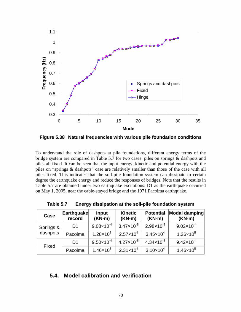
0.3

0.4

0.5

0.6

0.7

0.8

0.9

1

1.1

0 5 10 15 20 25 30 35

Mode

Freq

uenc

y (H

z)

Springs and dashpotsFixedHinge

Figure 5.38 Natural frequencies with various pile foundation conditions

To understand the role of dashpots at pile foundations, different energy terms of the bridge system are compared in Table 5.7 for two cases: piles on springs & dashpots and piles all fixed. It can be seen that the input energy, kinetic and potential energy with the piles on “springs & dashpots” case are relatively smaller than those of the case with all piles fixed. This indicates that the soil-pile foundation system can dissipate to certain degree the earthquake energy and reduce the responses of bridges. Note that the results in Table 5.7 are obtained under two earthquake excitations: D1 as the earthquake occurred on May 1, 2005, near the cable-stayed bridge and the 1971 Pacoima earthquake.

Table 5.7 Energy dissipation at the soil-pile foundation system

Case Earthquake record

Input (KN-m)

Kinetic (KN-m)

Potential (KN-m)

Modal damping(KN-m)

Springs & dashpots

D1 -49.08×10 -53.47×10 -52.98×10 -49.02×10

Pacoima 51.28×10 42.57×10 43.45×10 51.26×10

Fixed D1 -49.50×10 -54.27×10 -54.34×10 -49.42×10

Pacoima 51.46×10 42.31×10 43.10×10 51.46×10

5.4. Model calibration and verification

70

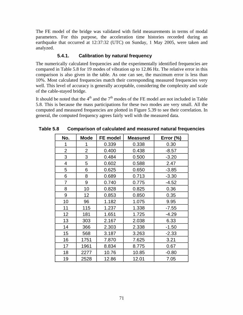
The FE model of the bridge was validated with field measurements in terms of modal parameters. For this purpose, the acceleration time histories recorded during an earthquake that occurred at 12:37:32 (UTC) on Sunday, 1 May 2005, were taken and analyzed.

5.4.1. Calibration by natural frequency The numerically calculated frequencies and the experimentally identified frequencies are compared in Table 5.8 for 19 modes of vibration up to 12.86 Hz. The relative error in this comparison is also given in the table. As one can see, the maximum error is less than 10%. Most calculated frequencies match their corresponding measured frequencies very well. This level of accuracy is generally acceptable, considering the complexity and scale of the cable-stayed bridge.

It should be noted that the 4th th and the 7 modes of the FE model are not included in Table 5.8. This is because the mass participations for these two modes are very small. All the computed and measured frequencies are plotted in Figure 5.39 to see their correlation. In general, the computed frequency agrees fairly well with the measured data.

Table 5.8 Comparison of calculated and measured natural frequencies

No. Mode FE model Measured Error (%) 1 1 0.339 0.338 0.30 2 2 0.400 0.438 -8.57 3 3 0.484 0.500 -3.20 4 5 0.602 0.588 2.47 5 6 0.625 0.650 -3.85 6 8 0.689 0.713 -3.30 7 9 0.740 0.775 -4.52 8 10 0.828 0.825 0.36 9 12 0.853 0.850 0.35 10 96 1.182 1.075 9.95 11 115 1.237 1.338 -7.55 12 181 1.651 1.725 -4.29 13 303 2.167 2.038 6.33 14 366 2.303 2.338 -1.50 15 568 3.187 3.263 -2.33 16 1751 7.870 7.625 3.21 17 1961 8.834 8.775 0.67 18 2277 10.76 10.85 -0.80 19 2528 12.86 12.01 7.05

71

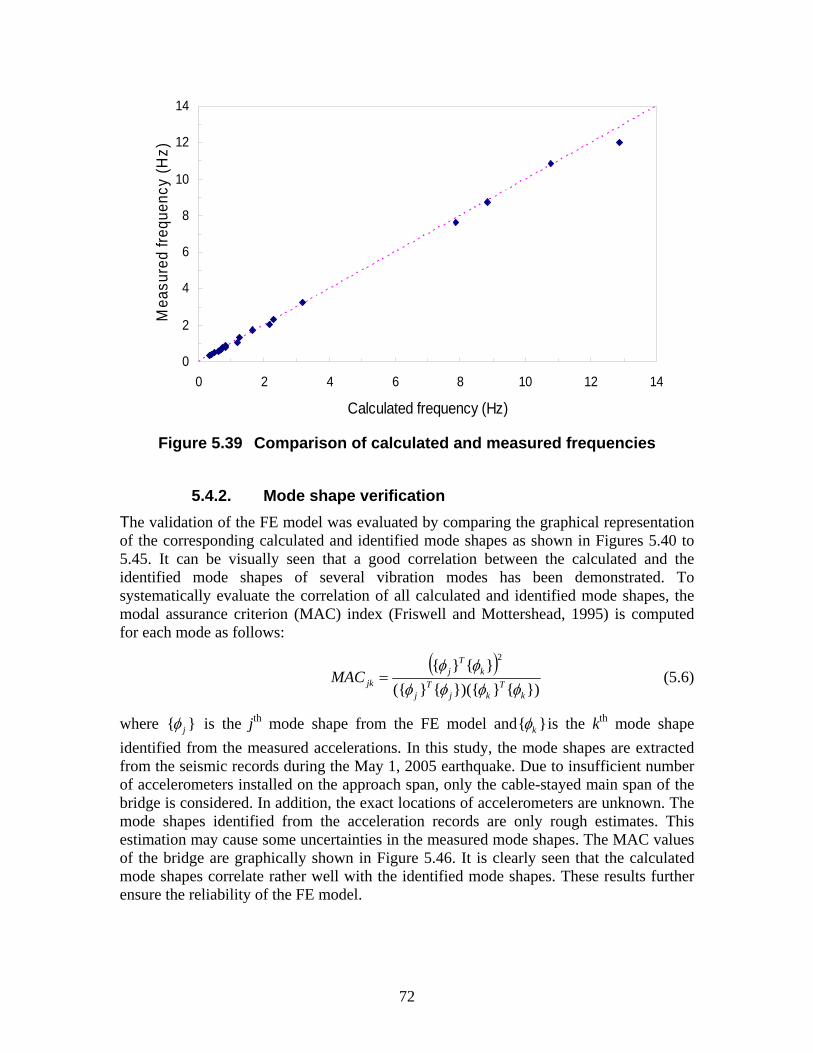
0

2

4

6

8

10

12

14

0 2 4 6 8 10 12 1

Calculated frequency (Hz)

Mea

sure

d fre

quen

cy (H

z)

4

Figure 5.39 Comparison of calculated and measured frequencies

5.4.2. Mode shape verification

The validation of the FE model was evaluated by comparing the graphical representation of the corresponding calculated and identified mode shapes as shown in Figures 5.40 to 5.45. It can be visually seen that a good correlation between the calculated and the identified mode shapes of several vibration modes has been demonstrated. To systematically evaluate the correlation of all calculated and identified mode shapes, the modal assurance criterion (MAC) index (Friswell and Mottershead, 1995) is computed for each mode as follows:

( ){φ }Tj {φk} 2

MAC jk = (5.6) ({φ j }

T {φ })({ }Tj φk {φk })

where { }φ th thj is the j mode shape from the FE model and{φk }is the k mode shape

identified from the measured accelerations. In this study, the mode shapes are extracted from the seismic records during the May 1, 2005 earthquake. Due to insufficient number of accelerometers installed on the approach span, only the cable-stayed main span of the bridge is considered. In addition, the exact locations of accelerometers are unknown. The mode shapes identified from the acceleration records are only rough estimates. This estimation may cause some uncertainties in the measured mode shapes. The MAC values of the bridge are graphically shown in Figure 5.46. It is clearly seen that the calculated mode shapes correlate rather well with the identified mode shapes. These results further ensure the reliability of the FE model.

72

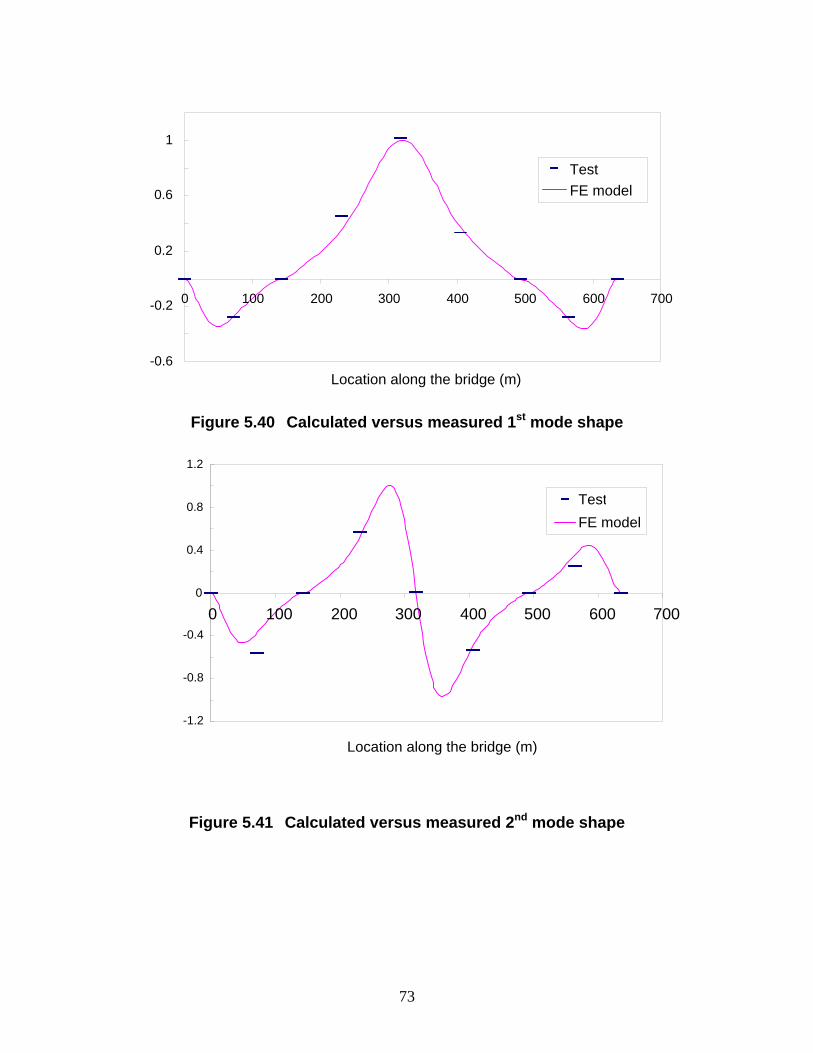
-0.6

-0.2

0.2

0.6

1

0 100 200 300 400 500 600 700

Location along the bridge (m)

TestFE model

Figure 5.40 Calculated versus measured 1st mode shape

-1.2

-0.8

-0.4

0

0.4

0.8

1.2

0 100 200 300 400 500 600 700

Location along the bridge (m)

TestFE model

Figure 5.41 Calculated versus measured 2nd mode shape

73

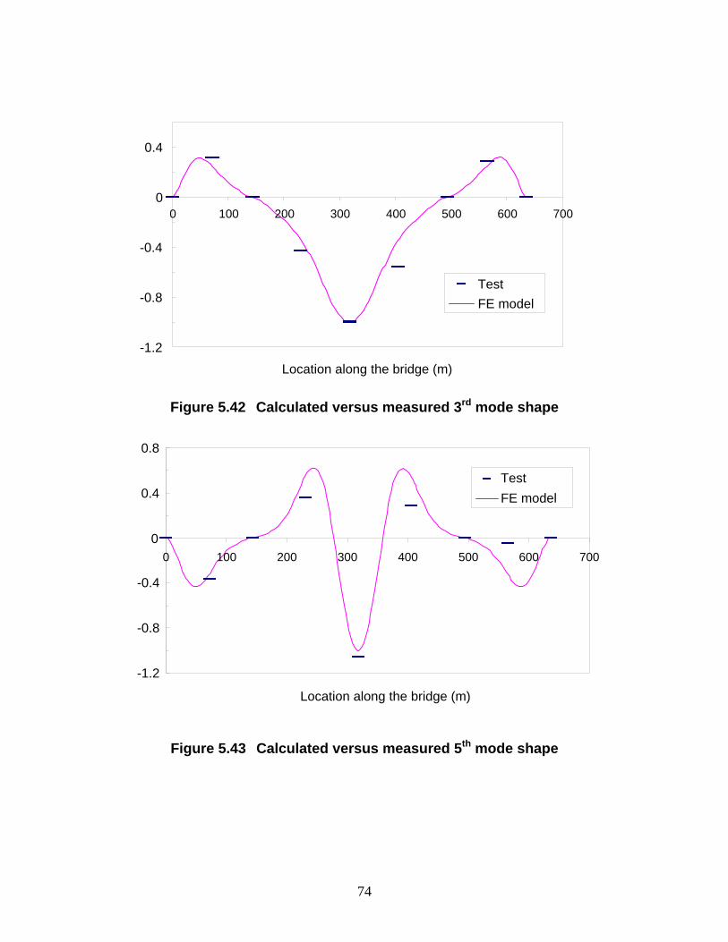
-1.2

-0.8

-0.4

0

0.4

0 100 200 300 400 500 600 700

Location along the bridge (m)

TestFE model

Figure 5.42 Calculated versus measured 3rd mode shape

-1.2

-0.8

-0.4

0

0.4

0.8

0 100 200 300 400 500 600 700

Location along the bridge (m)

Test FE model

Figure 5.43 Calculated versus measured 5th mode shape

74

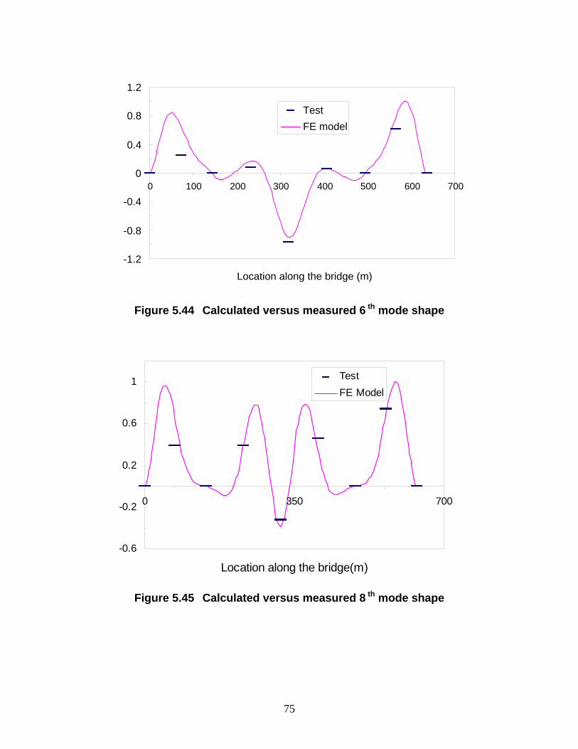
-1.2

-0.8

-0.4

0

0.4

0.8

1.2

0 100 200 300 400 500 600 700

Location along the bridge (m)

TestFE model

Figure 5.44 Calculated versus measured 6 th mode shape

-0.6

-0.2

0.2

0.6

1

0 350 700

Location along the bridge(m)

TestFE Model

Figure 5.45 Calculated versus measured 8 th mode shape

75

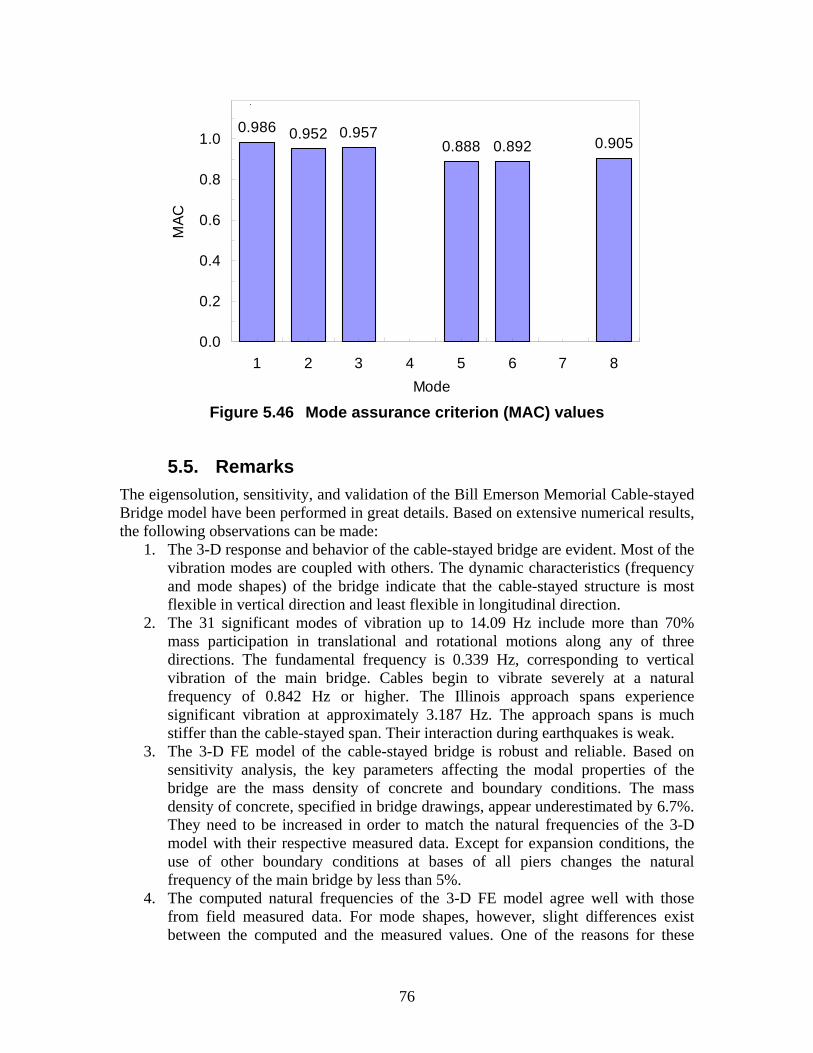
0.986 0.952 0.9570.888 0.892 0.905

0.0

0.2

0.4

0.6

0.8

1.0

1 2 3 4 5 6 7 8Mode

MAC

Figure 5.46 Mode assurance criterion (MAC) values

5.5. Remarks The eigensolution, sensitivity, and validation of the Bill Emerson Memorial Cable-stayed Bridge model have been performed in great details. Based on extensive numerical results, the following observations can be made:

1. The 3-D response and behavior of the cable-stayed bridge are evident. Most of the vibration modes are coupled with others. The dynamic characteristics (frequency and mode shapes) of the bridge indicate that the cable-stayed structure is most flexible in vertical direction and least flexible in longitudinal direction.

2. The 31 significant modes of vibration up to 14.09 Hz include more than 70% mass participation in translational and rotational motions along any of three directions. The fundamental frequency is 0.339 Hz, corresponding to vertical vibration of the main bridge. Cables begin to vibrate severely at a natural frequency of 0.842 Hz or higher. The Illinois approach spans experience significant vibration at approximately 3.187 Hz. The approach spans is much stiffer than the cable-stayed span. Their interaction during earthquakes is weak.

3. The 3-D FE model of the cable-stayed bridge is robust and reliable. Based on sensitivity analysis, the key parameters affecting the modal properties of the bridge are the mass density of concrete and boundary conditions. The mass density of concrete, specified in bridge drawings, appear underestimated by 6.7%. They need to be increased in order to match the natural frequencies of the 3-D model with their respective measured data. Except for expansion conditions, the use of other boundary conditions at bases of all piers changes the natural frequency of the main bridge by less than 5%.

4. The computed natural frequencies of the 3-D FE model agree well with those from field measured data. For mode shapes, however, slight differences exist between the computed and the measured values. One of the reasons for these

76

differences is that the exact locations of all accelerometers deployed on the bridge are unknown. Nevertheless, the mode assurance criterion index between a computed mode shape and its corresponding measured one is above 0.888 for the first eight modes. This indicates that the 3-D FE model is reasonable for engineering applications.

77

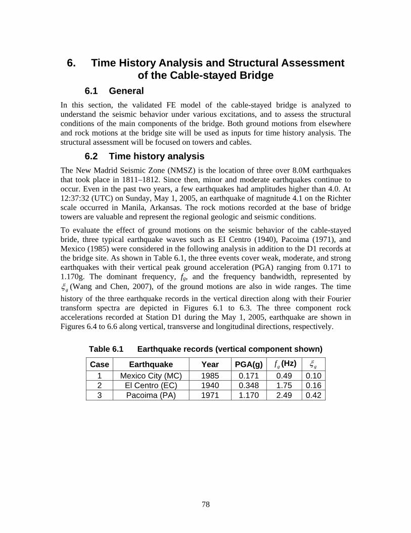
6. Time History Analysis and Structural Assessment of the Cable-stayed Bridge

6.1 General In this section, the validated FE model of the cable-stayed bridge is analyzed to understand the seismic behavior under various excitations, and to assess the structural conditions of the main components of the bridge. Both ground motions from elsewhere and rock motions at the bridge site will be used as inputs for time history analysis. The structural assessment will be focused on towers and cables.

6.2 Time history analysis The New Madrid Seismic Zone (NMSZ) is the location of three over 8.0M earthquakes that took place in 1811–1812. Since then, minor and moderate earthquakes continue to occur. Even in the past two years, a few earthquakes had amplitudes higher than 4.0. At 12:37:32 (UTC) on Sunday, May 1, 2005, an earthquake of magnitude 4.1 on the Richter scale occurred in Manila, Arkansas. The rock motions recorded at the base of bridge towers are valuable and represent the regional geologic and seismic conditions.

To evaluate the effect of ground motions on the seismic behavior of the cable-stayed bride, three typical earthquake waves such as EI Centro (1940), Pacoima (1971), and Mexico (1985) were considered in the following analysis in addition to the D1 records at the bridge site. As shown in Table 6.1, the three events cover weak, moderate, and strong earthquakes with their vertical peak ground acceleration (PGA) ranging from 0.171 to 1.170g. The dominant frequency, fg, and the frequency bandwidth, represented by ξg (Wang and Chen, 2007), of the ground motions are also in wide ranges. The time history of the three earthquake records in the vertical direction along with their Fourier transform spectra are depicted in Figures 6.1 to 6.3. The three component rock accelerations recorded at Station D1 during the May 1, 2005, earthquake are shown in Figures 6.4 to 6.6 along vertical, transverse and longitudinal directions, respectively.

Table 6.1 Earthquake records (vertical component shown)

Case Earthquake Year PGA(g) f (Hz) g ξ g

1 Mexico City (MC) 1985 0.171 0.49 0.10 2 El Centro (EC) 1940 0.348 1.75 0.16 3 Pacoima (PA) 1971 1.170 2.49 0.42

78

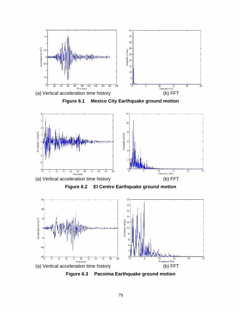
(a) Vertical acceleration time history (b) FFT

Figure 6.1 Mexico City Earthquake ground motion

(a) Vertical acceleration time history (b) FFT

Figure 6.2 El Centro Earthquake ground motion

(a) Vertical acceleration time history (b) FFT

Figure 6.3 Pacoima Earthquake ground motion

79

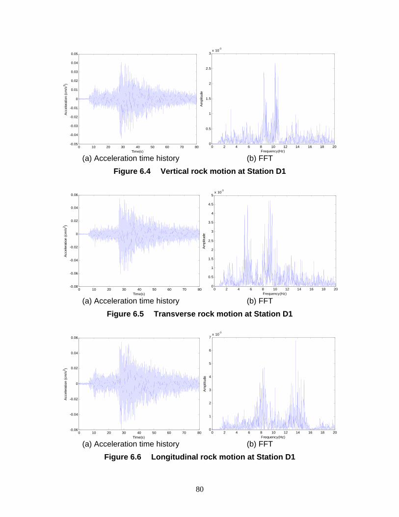
0 2 4 6 8 10 12 14 16 18 200

0.5

1

1.5

2

2.5

3x 10-3

Frequency(Hz)

Am

plitu

de

0 10 20 30 40 50 60 70 80-0.05

-0.04

-0.03

-0.02

-0.01

0

0.01

0.02

0.03

0.04

0.05

Time(s)

Acc

eler

atio

n (c

m/s

2 )

(a) Acceleration time history (b) FFT

Figure 6.4 Vertical rock motion at Station D1

0 10 20 30 40 50 60 70 80-0.08

-0.06

-0.04

-0.02

0

0.02

0.04

0.06

Time(s)

Acc

eler

atio

n (c

m/s

2 )

0 2 4 6 8 10 12 14 16 18 200

0.5

1

1.5

2

2.5

3

3.5

4

4.5

5x 10-3

Frequency(Hz)

Am

plitu

de

(a) Acceleration time history (b) FFT

Figure 6.5 Transverse rock motion at Station D1

0 2 4 6 8 10 12 14 16 18 200

1

2

3

4

5

6

7x 10-3

Frequency(Hz)

Am

plitu

de

0 10 20 30 40 50 60 70 80-0.06

-0.04

-0.02

0

0.02

0.04

0.06

Time(s)

Acc

eler

atio

n (c

m/s

2 )

(a) Acceleration time history (b) FFT

Figure 6.6 Longitudinal rock motion at Station D1

80

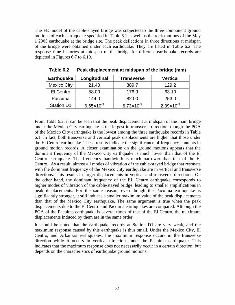
The FE model of the cable-stayed bridge was subjected to the three-component ground motions of each earthquake specified in Table 6.1 as well as the rock motions of the May 1 2005 earthquake at the bridge site. The peak deflections in three directions at midspan of the bridge were obtained under each earthquake. They are listed in Table 6.2. The response time histories at midspan of the bridge for different earthquake records are depicted in Figures 6.7 to 6.10.

Table 6.2 Peak displacement at midspan of the bridge (mm)

Earthquake Longitudinal Transverse Vertical Mexico City 21.40 389.7 129.2 El Centro 58.00 176.9 63.10 Pacoima 144.0 82.00 253.0

Station D1 -36.65×10 -36.73×10 -32.39×10

From Table 6.2, it can be seen that the peak displacement at midspan of the main bridge under the Mexico City earthquake is the largest in transverse direction, though the PGA of the Mexico City earthquake is the lowest among the three earthquake records in Table 6.1. In fact, both transverse and vertical peak displacements are higher that those under the El Centro earthquake. These results indicate the significance of frequency contents in ground motion records. A closer examination on the ground motions appears that the dominant frequency of the Mexico City earthquake is much lower than that of the El Centro earthquake. The frequency bandwidth is much narrower than that of the El Centro. As a result, almost all modes of vibration of the cable-stayed bridge that resonate with the dominant frequency of the Mexico City earthquake are in vertical and transverse directions. This results in larger displacements in vertical and transverse directions. On the other hand, the dominant frequency of the EL Centro earthquake corresponds to higher modes of vibration of the cable-stayed bridge, leading to smaller amplifications in peak displacements. For the same reason, even though the Pacoima earthquake is significantly stronger, it still induces a smaller maximum value of the peak displacements than that of the Mexico City earthquake. The same argument is true when the peak displacements due to the El Centro and Pacoima earthquakes are compared. Although the PGA of the Pacoima earthquake is several times of that of the El Centro, the maximum displacements induced by them are in the same order.

It should be noted that the earthquake records at Station D1 are very weak, and the maximum response caused by this earthquake is thus small. Under the Mexico City, El Centro, and Arkansas earthquakes, the maximum response occurs in the transverse direction while it occurs in vertical direction under the Pacoima earthquake. This indicates that the maximum response does not necessarily occur in a certain direction, but depends on the characteristics of earthquake ground motions.

81

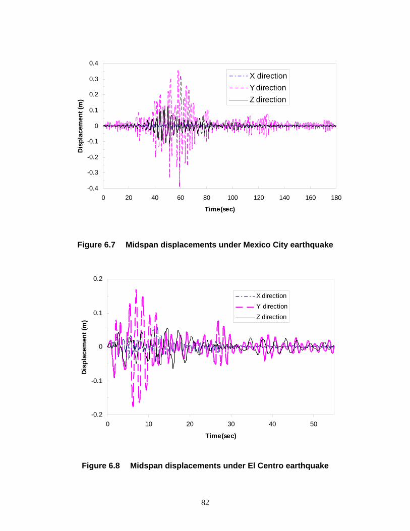
-0.4

-0.3

-0.2

-0.1

0

0.1

0.2

0.3

0.4

0 20 40 60 80 100 120 140 160 180

Time(sec)

Disp

lace

men

t (m

)X directionY directionZ direction

Figure 6.7 Midspan displacements under Mexico City earthquake

-0.2

-0.1

0

0.1

0.2

0 10 20 30 40 50

Time(sec)

Dis

plac

emen

t (m

)

X directionY directionZ direction

Figure 6.8 Midspan displacements under El Centro earthquake

82

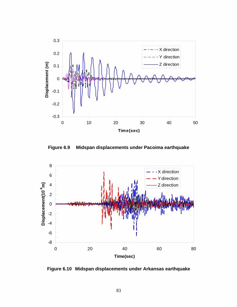
-0.3

-0.2

-0.1

0

0.1

0.2

0.3

0 10 20 30 40

Time(sec)

Dis

plac

emen

t (m

)X direction

Y direction

Z direction

50

Figure 6.9 Midspan displacements under Pacoima earthquake

-8

-6

-4

-2

0

2

4

6

8

0 20 40 60 8

Time(sec)

Dis

plac

emen

t(10-6

m)

X directionY directionZ direction

0

Figure 6.10 Midspan displacements under Arkansas earthquake

83

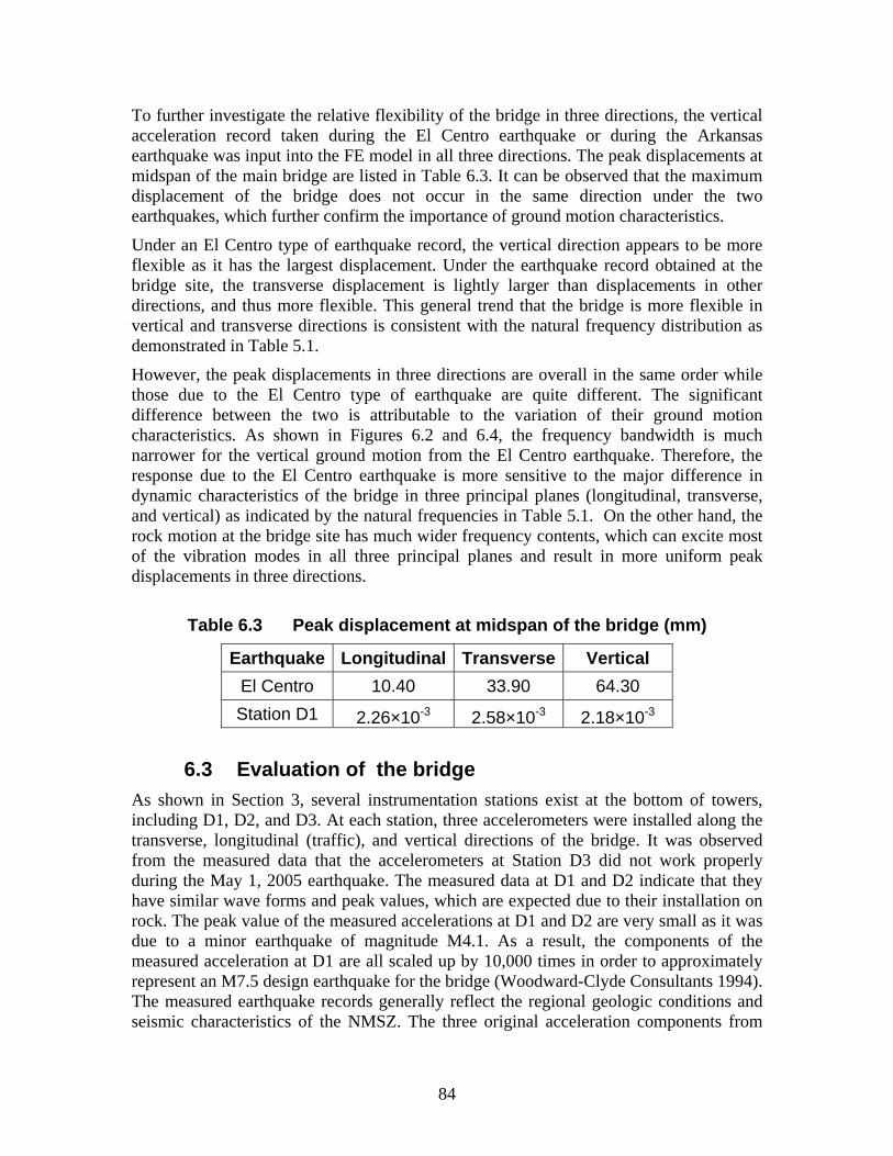
To further investigate the relative flexibility of the bridge in three directions, the vertical acceleration record taken during the El Centro earthquake or during the Arkansas earthquake was input into the FE model in all three directions. The peak displacements at midspan of the main bridge are listed in Table 6.3. It can be observed that the maximum displacement of the bridge does not occur in the same direction under the two earthquakes, which further confirm the importance of ground motion characteristics.

Under an El Centro type of earthquake record, the vertical direction appears to be more flexible as it has the largest displacement. Under the earthquake record obtained at the bridge site, the transverse displacement is lightly larger than displacements in other directions, and thus more flexible. This general trend that the bridge is more flexible in vertical and transverse directions is consistent with the natural frequency distribution as demonstrated in Table 5.1.

However, the peak displacements in three directions are overall in the same order while those due to the El Centro type of earthquake are quite different. The significant difference between the two is attributable to the variation of their ground motion characteristics. As shown in Figures 6.2 and 6.4, the frequency bandwidth is much narrower for the vertical ground motion from the El Centro earthquake. Therefore, the response due to the El Centro earthquake is more sensitive to the major difference in dynamic characteristics of the bridge in three principal planes (longitudinal, transverse, and vertical) as indicated by the natural frequencies in Table 5.1. On the other hand, the rock motion at the bridge site has much wider frequency contents, which can excite most of the vibration modes in all three principal planes and result in more uniform peak displacements in three directions.

Table 6.3 Peak displacement at midspan of the bridge (mm)

Earthquake Longitudinal Transverse Vertical El Centro 10.40 33.90 64.30 Station D1 -32.26×10 -32.58×10 2.18×10-3

6.3 Evaluation of the bridge As shown in Section 3, several instrumentation stations exist at the bottom of towers, including D1, D2, and D3. At each station, three accelerometers were installed along the transverse, longitudinal (traffic), and vertical directions of the bridge. It was observed from the measured data that the accelerometers at Station D3 did not work properly during the May 1, 2005 earthquake. The measured data at D1 and D2 indicate that they have similar wave forms and peak values, which are expected due to their installation on rock. The peak value of the measured accelerations at D1 and D2 are very small as it was due to a minor earthquake of magnitude M4.1. As a result, the components of the measured acceleration at D1 are all scaled up by 10,000 times in order to approximately represent an M7.5 design earthquake for the bridge (Woodward-Clyde Consultants 1994). The measured earthquake records generally reflect the regional geologic conditions and seismic characteristics of the NMSZ. The three original acceleration components from

84

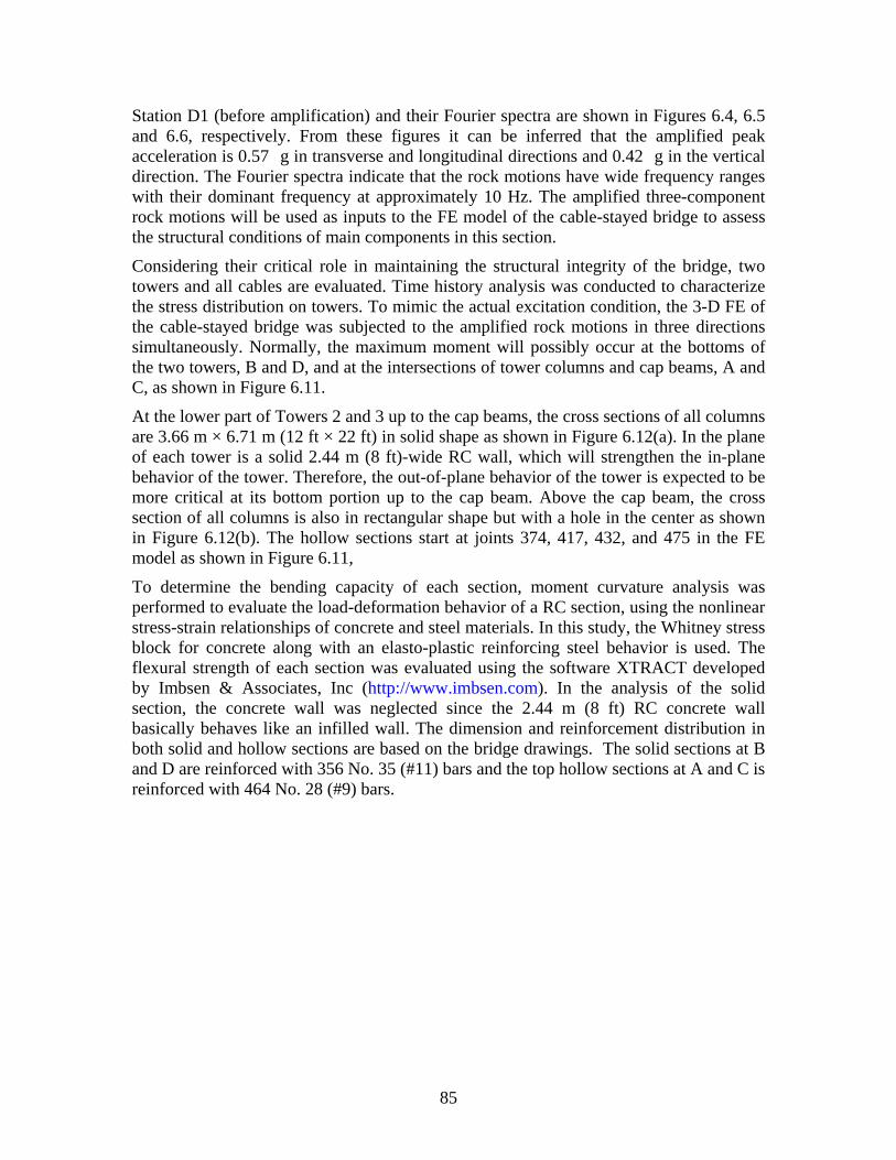
Station D1 (before amplification) and their Fourier spectra are shown in Figures 6.4, 6.5 and 6.6, respectively. From these figures it can be inferred that the amplified peak acceleration is 0.57 g in transverse and longitudinal directions and 0.42 g in the vertical direction. The Fourier spectra indicate that the rock motions have wide frequency ranges with their dominant frequency at approximately 10 Hz. The amplified three-component rock motions will be used as inputs to the FE model of the cable-stayed bridge to assess the structural conditions of main components in this section.

Considering their critical role in maintaining the structural integrity of the bridge, two towers and all cables are evaluated. Time history analysis was conducted to characterize the stress distribution on towers. To mimic the actual excitation condition, the 3-D FE of the cable-stayed bridge was subjected to the amplified rock motions in three directions simultaneously. Normally, the maximum moment will possibly occur at the bottoms of the two towers, B and D, and at the intersections of tower columns and cap beams, A and C, as shown in Figure 6.11.

At the lower part of Towers 2 and 3 up to the cap beams, the cross sections of all columns are 3.66 m × 6.71 m (12 ft × 22 ft) in solid shape as shown in Figure 6.12(a). In the plane of each tower is a solid 2.44 m (8 ft)-wide RC wall, which will strengthen the in-plane behavior of the tower. Therefore, the out-of-plane behavior of the tower is expected to be more critical at its bottom portion up to the cap beam. Above the cap beam, the cross section of all columns is also in rectangular shape but with a hole in the center as shown in Figure 6.12(b). The hollow sections start at joints 374, 417, 432, and 475 in the FE model as shown in Figure 6.11,

To determine the bending capacity of each section, moment curvature analysis was performed to evaluate the load-deformation behavior of a RC section, using the nonlinear stress-strain relationships of concrete and steel materials. In this study, the Whitney stress block for concrete along with an elasto-plastic reinforcing steel behavior is used. The flexural strength of each section was evaluated using the software XTRACT developed by Imbsen & Associates, Inc (http://www.imbsen.com). In the analysis of the solid section, the concrete wall was neglected since the 2.44 m (8 ft) RC concrete wall basically behaves like an infilled wall. The dimension and reinforcement distribution in both solid and hollow sections are based on the bridge drawings. The solid sections at B and D are reinforced with 356 No. 35 (#11) bars and the top hollow sections at A and C is reinforced with 464 No. 28 (#9) bars.

85

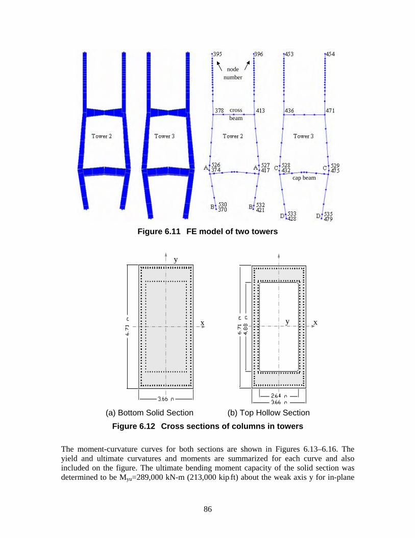
node number

cross beam

cap beam

Figure 6.11 FE model of two towers

(a) Bottom Solid Section (b) Top Hollow Section

y

y xx

Figure 6.12 Cross sections of columns in towers

The moment-curvature curves for both sections are shown in Figures 6.13–6.16. The yield and ultimate curvatures and moments are summarized for each curve and also included on the figure. The ultimate bending moment capacity of the solid section was determined to be Myu=289,000 kN-m (213,000 kip-ft) about the weak axis y for in-plane

86

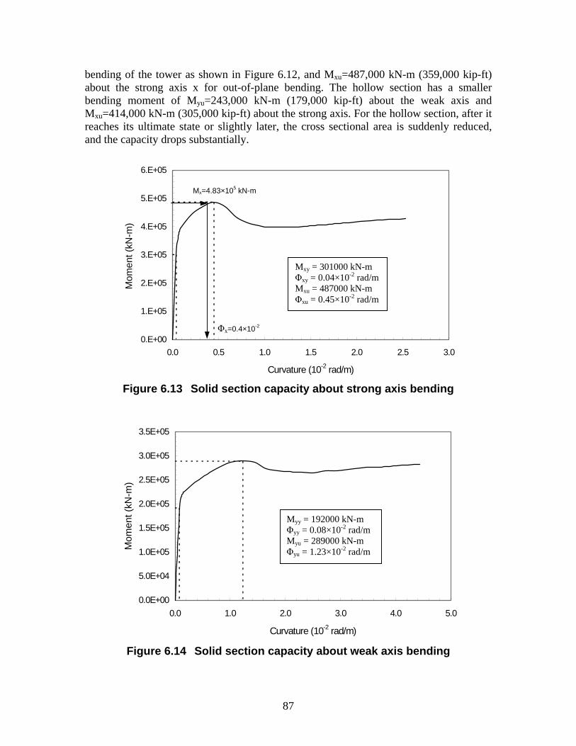
bending of the tower as shown in Figure 6.12, and Mxu=487,000 kN-m (359,000 kip-ft) about the strong axis x for out-of-plane bending. The hollow section has a smaller bending moment of Myu=243,000 kN-m (179,000 kip-ft) about the weak axis and Mxu=414,000 kN-m (305,000 kip-ft) about the strong axis. For the hollow section, after it reaches its ultimate state or slightly later, the cross sectional area is suddenly reduced, and the capacity drops substantially.

0.E+00

1.E+05

2.E+05

3.E+05

4.E+05

5.E+05

6.E+05

0.0 0.5 1.0 1.5 2.0 2.5 3.0

Curvature (10-2 rad/m)

Mom

ent (

kN-m

)

Mx=4.83×105 kN-m

Φx=0.4×10-2

Mxy = 301000 kN-m Φxy = 0.04×10-2 rad/mMxu = 487000 kN-m Φxu = 0.45×10-2 rad/m

Figure 6.13 Solid section capacity about strong axis bending

0.0E+00

5.0E+04

1.0E+05

1.5E+05

2.0E+05

2.5E+05

3.0E+05

3.5E+05

0.0 1.0 2.0 3.0 4.0 5.0

Curvature (10-2 rad/m)

Mom

ent (

kN-m

)

Myy = 192000 kN-m Φ = 0.08×10-2 rad/m yy

= 289000 kN-m Myu = 1.23×10-2 rad/m Φyu

Figure 6.14 Solid section capacity about weak axis bending

87

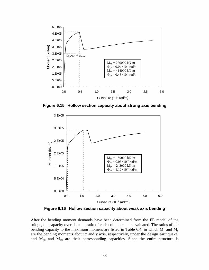
0.E+00

5.E+04

1.E+05

2.E+05

2.E+05

3.E+05

3.E+05

4.E+05

4.E+05

5.E+05

0.0 0.5 1.0 1.5 2.0 2.5 3.0

Curvature (10-2 rad/m)

Mom

ent (

kN-m

)

Mxy = 250000 kN-m Φxy = 0.04×10-2 rad/mMxu = 414000 kN-m Φxu = 0.48×10-2 rad/m

M =3×105 kN-mx

Figure 6.15 Hollow section capacity about strong axis bending

0.E+00

5.E+04

1.E+05

2.E+05

2.E+05

3.E+05

3.E+05

0.0 1.0 2.0 3.0 4.0 5.0 6.0

Curvature (10-2 rad/m)

Mom

ent (

kN-m

)

Myy = 159000 kN-m Φyy = 0.08×10-2 rad/m Myu = 243000 kN-m Φyu = 1.12×10-2 rad/m

Figure 6.16 Hollow section capacity about weak axis bending

After the bending moment demands have been determined from the FE model of the bridge, the capacity over demand ratio of each column can be evaluated. The ratios of the bending capacity to the maximum moment are listed in Table 6.4, in which Mx and My are the bending moments about x and y axis, respectively, under the design earthquake, and Mxu and Myu are their corresponding capacities. Since the entire structure is

88

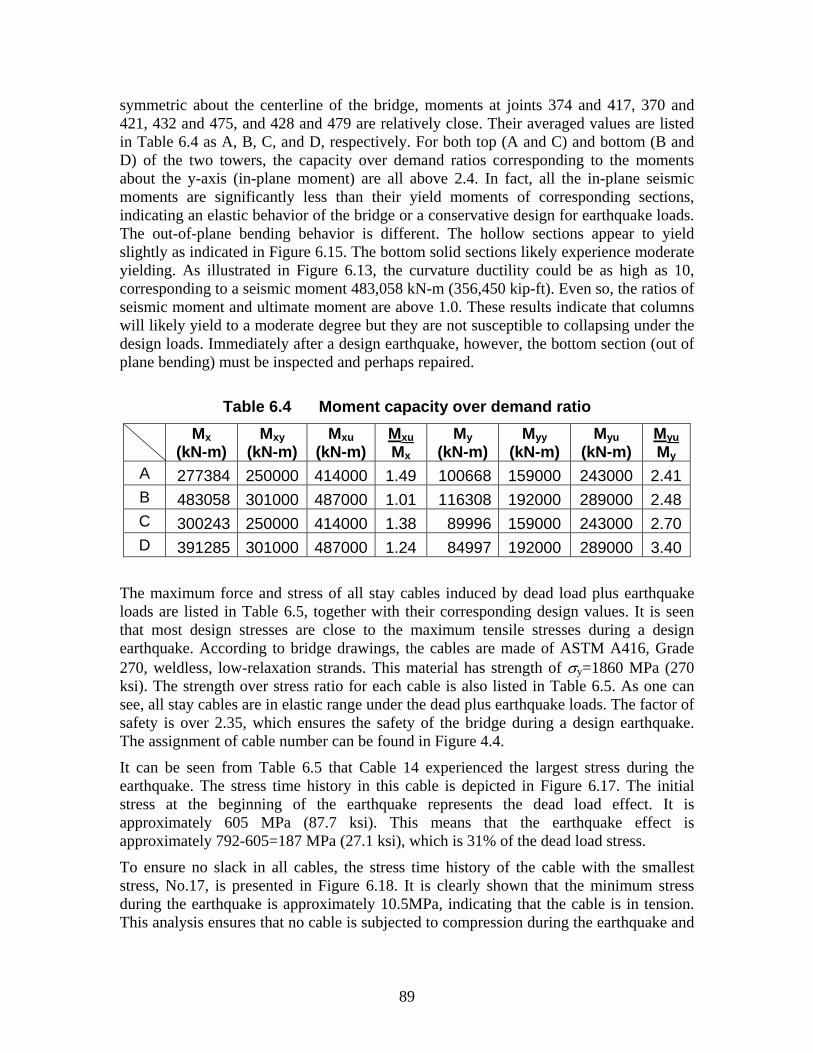
symmetric about the centerline of the bridge, moments at joints 374 and 417, 370 and 421, 432 and 475, and 428 and 479 are relatively close. Their averaged values are listed in Table 6.4 as A, B, C, and D, respectively. For both top (A and C) and bottom (B and D) of the two towers, the capacity over demand ratios corresponding to the moments about the y-axis (in-plane moment) are all above 2.4. In fact, all the in-plane seismic moments are significantly less than their yield moments of corresponding sections, indicating an elastic behavior of the bridge or a conservative design for earthquake loads. The out-of-plane bending behavior is different. The hollow sections appear to yield slightly as indicated in Figure 6.15. The bottom solid sections likely experience moderate yielding. As illustrated in Figure 6.13, the curvature ductility could be as high as 10, corresponding to a seismic moment 483,058 kN-m (356,450 kip-ft). Even so, the ratios of seismic moment and ultimate moment are above 1.0. These results indicate that columns will likely yield to a moderate degree but they are not susceptible to collapsing under the design loads. Immediately after a design earthquake, however, the bottom section (out of plane bending) must be inspected and perhaps repaired.

Table 6.4 Moment capacity over demand ratio

Mx (kN-m)

Mxy (kN-m)

Mxu (kN-m)

MxuMx

My (kN-m)

Myy (kN-m)

Myu (kN-m)

MyuMy

A 277384 250000 414000 1.49 100668 159000 243000 2.41B 483058 301000 487000 1.01 116308 192000 289000 2.48C 300243 250000 414000 1.38 89996 159000 243000 2.70D 391285 301000 487000 1.24 84997 192000 289000 3.40

The maximum force and stress of all stay cables induced by dead load plus earthquake loads are listed in Table 6.5, together with their corresponding design values. It is seen that most design stresses are close to the maximum tensile stresses during a design earthquake. According to bridge drawings, the cables are made of ASTM A416, Grade 270, weldless, low-relaxation strands. This material has strength of σy=1860 MPa (270 ksi). The strength over stress ratio for each cable is also listed in Table 6.5. As one can see, all stay cables are in elastic range under the dead plus earthquake loads. The factor of safety is over 2.35, which ensures the safety of the bridge during a design earthquake. The assignment of cable number can be found in Figure 4.4.

It can be seen from Table 6.5 that Cable 14 experienced the largest stress during the earthquake. The stress time history in this cable is depicted in Figure 6.17. The initial stress at the beginning of the earthquake represents the dead load effect. It is approximately 605 MPa (87.7 ksi). This means that the earthquake effect is approximately 792-605=187 MPa (27.1 ksi), which is 31% of the dead load stress.

To ensure no slack in all cables, the stress time history of the cable with the smallest stress, No.17, is presented in Figure 6.18. It is clearly shown that the minimum stress during the earthquake is approximately 10.5MPa, indicating that the cable is in tension. This analysis ensures that no cable is subjected to compression during the earthquake and

89

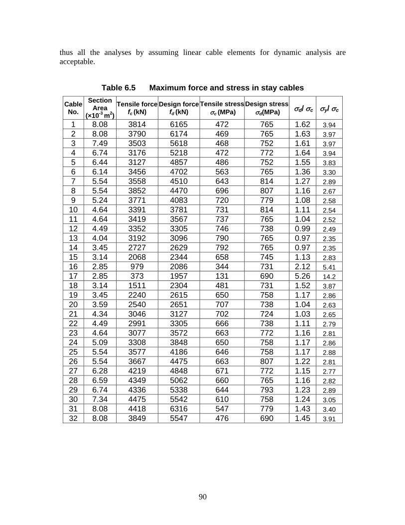
90

thus all the analyses by assuming linear cable elements for dynamic analysis are acceptable.

Table 6.5 Maximum force and stress in stay cables

Cable No.

Section Area

(×10-3 m2) Tensile force

fc (kN) Design force

fd (kN) Tensile stress

σc (MPa) Design stress

σd(MPa) σd/ σc σy/ σc

1 8.08 3814 6165 472 765 1.62 3.94 2 8.08 3790 6174 469 765 1.63 3.97 3 7.49 3503 5618 468 752 1.61 3.97 4 6.74 3176 5218 472 772 1.64 3.94 5 6.44 3127 4857 486 752 1.55 3.83 6 6.14 3456 4702 563 765 1.36 3.30 7 5.54 3558 4510 643 814 1.27 2.89 8 5.54 3852 4470 696 807 1.16 2.67 9 5.24 3771 4083 720 779 1.08 2.58

10 4.64 3391 3781 731 814 1.11 2.54 11 4.64 3419 3567 737 765 1.04 2.52 12 4.49 3352 3305 746 738 0.99 2.49 13 4.04 3192 3096 790 765 0.97 2.35 14 3.45 2727 2629 792 765 0.97 2.35 15 3.14 2068 2344 658 745 1.13 2.83 16 2.85 979 2086 344 731 2.12 5.41 17 2.85 373 1957 131 690 5.26 14.2 18 3.14 1511 2304 481 731 1.52 3.87 19 3.45 2240 2615 650 758 1.17 2.86 20 3.59 2540 2651 707 738 1.04 2.63 21 4.34 3046 3127 702 724 1.03 2.65 22 4.49 2991 3305 666 738 1.11 2.79 23 4.64 3077 3572 663 772 1.16 2.81 24 5.09 3308 3848 650 758 1.17 2.86 25 5.54 3577 4186 646 758 1.17 2.88 26 5.54 3667 4475 663 807 1.22 2.81 27 6.28 4219 4848 671 772 1.15 2.77 28 6.59 4349 5062 660 765 1.16 2.82 29 6.74 4336 5338 644 793 1.23 2.89 30 7.34 4475 5542 610 758 1.24 3.05 31 8.08 4418 6316 547 779 1.43 3.40 32 8.08 3849 5547 476 690 1.45 3.91

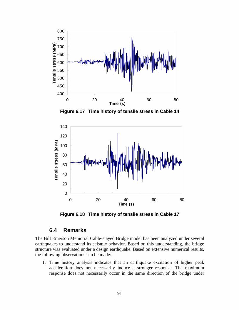
400

450

500

550

600

650

700

750

800

0 20 40 60 8Time (s)

Tens

ile s

tres

s (M

Pa)

0

Figure 6.17 Time history of tensile stress in Cable 14

0

20

40

60

80

100

120

140

0 20 40 60 8Time (s)

Tens

ile s

tres

s (M

Pa)

0

Figure 6.18 Time history of tensile stress in Cable 17

6.4 Remarks The Bill Emerson Memorial Cable-stayed Bridge model has been analyzed under several earthquakes to understand its seismic behavior. Based on this understanding, the bridge structure was evaluated under a design earthquake. Based on extensive numerical results, the following observations can be made:

1. Time history analysis indicates that an earthquake excitation of higher peak acceleration does not necessarily induce a stronger response. The maximum response does not necessarily occur in the same direction of the bridge under

91

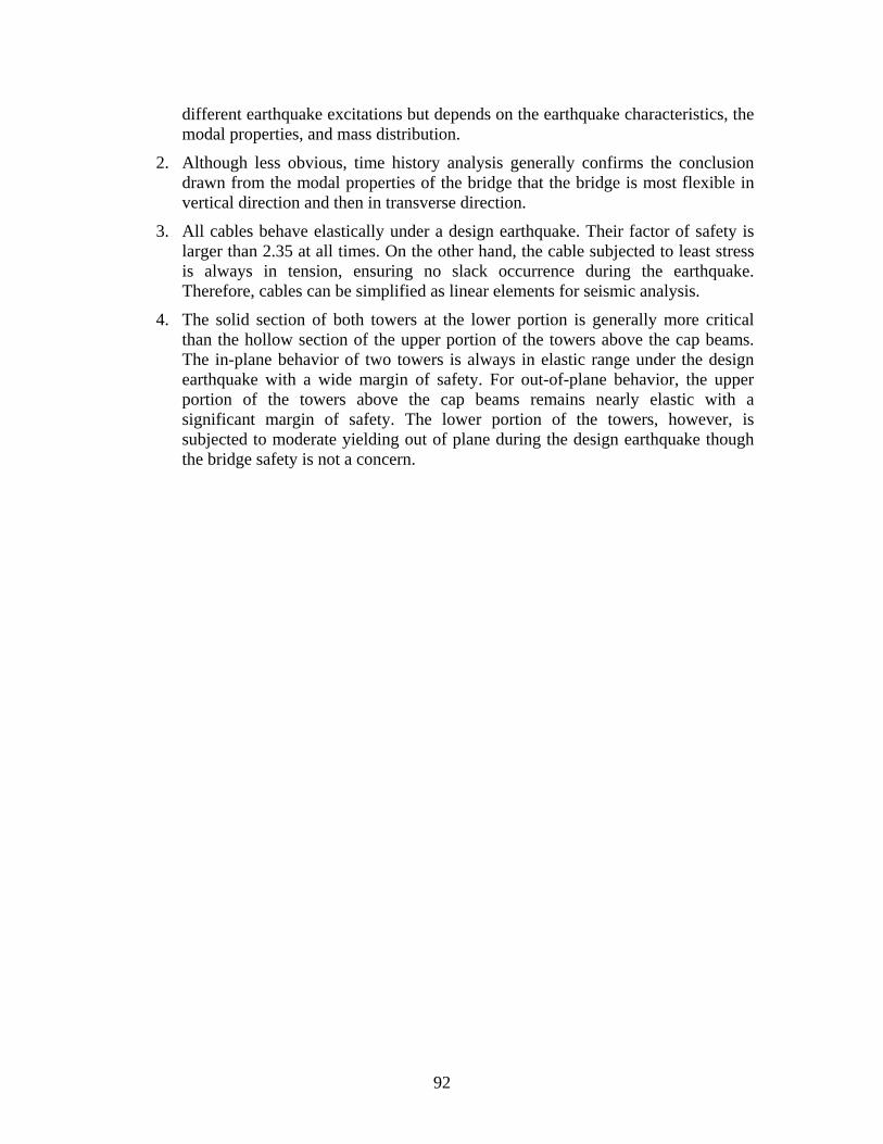
different earthquake excitations but depends on the earthquake characteristics, the modal properties, and mass distribution.

2. Although less obvious, time history analysis generally confirms the conclusion drawn from the modal properties of the bridge that the bridge is most flexible in vertical direction and then in transverse direction.

3. All cables behave elastically under a design earthquake. Their factor of safety is larger than 2.35 at all times. On the other hand, the cable subjected to least stress is always in tension, ensuring no slack occurrence during the earthquake. Therefore, cables can be simplified as linear elements for seismic analysis.

4. The solid section of both towers at the lower portion is generally more critical than the hollow section of the upper portion of the towers above the cap beams. The in-plane behavior of two towers is always in elastic range under the design earthquake with a wide margin of safety. For out-of-plane behavior, the upper portion of the towers above the cap beams remains nearly elastic with a significant margin of safety. The lower portion of the towers, however, is subjected to moderate yielding out of plane during the design earthquake though the bridge safety is not a concern.

92

7. Conclusions and Recommendations Bill Emerson Memorial Cable-stayed Bridge is one of very few long-span bridges in the U.S. that are instrumented with a real-time seismic monitoring system. This system consists of 84 accelerometers deployed on the bridge and on two nearby free fields. Based on the traffic and earthquake data, this study mainly develops and validates a realistic 3-D FE model of the bridge as well as assesses the seismic condition of the bridge under a projected design earthquake.

7.1 Main findings The main topics addressed in this report include: (1) automatic retrieval of peak accelerations and measured data analysis, (2) 3-D FE bridge model with explicit modeling of all main components, (3) sensitivity study and validation of the 3-D FE bridge model, and (4) seismic behavior and assessment of the bridge structure. Based on the comprehensive analysis of the cable-stayed bridge, the following conclusions can be drawn:

1. A Java-based system was developed to automatically compile the peak ground and structural accelerations measured from the bridge. The system can be seamlessly integrated with the data management system at the ISIS website. The output of this system is a string of peak acceleration data every hour or other time windows, which can be pulled into an Excel sheet for further processing.

2. The peak-picking method in frequency domain can be conveniently applied to analyze a huge set of field measured data from the seismic monitoring system. The vibration characteristics of the bridge such as natural frequencies and mode shapes were extracted.

3. One rigid link element must be introduced in the FE model at each end of a cable in order to model the actual length and configuration of the cable as specified in as-built drawings. Cables significantly influence the stiffness of the bridge system. Their sagging should be taken into account in the modeling of the cable-stayed bridge to account for geometric nonlinear effects.

4. Extra attention must be paid to the modeling process of bearings at each pier both in the main span and in the approach span of the bridge. They play an important role in seismic behaviors of the complex cable-stayed bridge.

5. The 3-D response and behavior of the cable-stayed bridge are evident. Most of the vibration modes are coupled with others. The dynamic characteristics (frequency and mode shapes) of the bridge indicate that the cable-stayed structure is most flexible in vertical direction and least flexible in longitudinal direction. This observation is generally supported by time history analysis.

6. The 31 significant modes of vibration up to 14.09 Hz include more than 70% mass participation in translational and rotational motions along any of three directions. The fundamental frequency is 0.339 Hz, corresponding to vertical vibration of the main bridge. Cables begin to vibrate severely at a natural frequency of 0.842 Hz or higher. The Illinois approach spans experience

93

significant vibration at approximately 3.187 Hz. The approach spans is much stiffer than the cable-stayed span. Their interaction during earthquakes is weak.

7. Based on sensitivity analysis, the key parameters affecting the modal properties of the bridge are the mass density of concrete and boundary conditions. The mass density of concrete, specified in bridge drawings, appear underestimated by 6.7%. They need to be increased in order to match the natural frequencies of the 3-D model with their respective measured data. Except for expansion conditions, the use of other boundary conditions at bases of all piers changes the natural frequency of the main bridge by less than 5%.

8. The computed natural frequencies of the 3-D FE model agree well with those from field measured data. The maximum error of the first 31 significant modes is within 10%. For mode shapes, however, slight differences exist between the computed and the measured values. One of the reasons for these differences is that the exact locations of all accelerometers deployed on the bridge are unknown. Nevertheless, the mode assurance criterion index between a computed mode shape and its corresponding measured one is above 0.888 for the first eight modes. This indicates that the 3-D FE model is fairly accurate for engineering applications.

9. Time history analysis indicates that an earthquake excitation of higher peak acceleration does not necessarily induce a stronger response. The maximum response does not necessarily occur in the same direction of the bridge under different earthquake excitations but depends on the earthquake characteristics, the modal properties, and mass distribution.

10. All cables behave elastically under a design earthquake. Their factor of safety is larger than 2.35 at all times. On the other hand, the cable subjected to least stress is always in tension, ensuring no slack occurrence during the earthquake. Therefore, cables can be simplified as linear elements for seismic analysis.

11. The solid section of both towers at the lower portion is generally more critical than the hollow section of the upper portion above the cap beams. The in-plane behavior of two towers is always in elastic range under the design earthquake with a wide margin of safety. Similarly, for out-of-plane behavior, the upper portion of the towers above the cap beams remains nearly elastic with a significant margin of safety. The lower portion of the towers, however, likely experiences moderate yielding out of plane during the design earthquake though the safety of the bridge is not a concern.

7.2 Future research The seismic instrumentation system was installed and put in operation in December 2004. Since then, acceleration data from ambient vibration have been collected continuously from the Bill Emerson Memorial Cable-stayed Bridge. The current study only addressed one way of using these data for structural assessment of the bridge under a projected design earthquake.

94

The vast arrays of acceleration data can also be used to address a number of issues related to engineering seismology, engineering design, bridge maintenance, bridge security, and bridge management. In a long term, these potential uses include, but are not limited to,

1. Assess the bridge structural condition in near real time to compliment the mandatory once-every-two-years inspections of the bridge so that the problem areas, if any, can be readily probed and examined in a cost-effective way.

2. Evaluate the bridge structural condition in a short time immediately after a catastrophic earthquake event to assist in decision making for emergency traffic uses or general public transportation in a much shorter time than traditional visual inspections may take.

3. Validate design assumptions made during the design of the cabled-stayed bridge. Several structure details are unique features to the Bill Emerson Memorial Bridge. Due to complexity and large scale of the Bridge, these unique features generally cannot be validated to the full extent with laboratory tests. The acceleration data measured from the bridge are valuable to accomplishing this important engineering task.

4. Collect the load data of small and moderate earthquakes for bridges in the Central United States and study the free field response of soil deposits and the spatial distribution of ground motions.

5. Monitor the security and safety of the critical transportation system in combination with other visual tools that may be installed in the future such as blast effects and vehicle impact.

This study provides a 3-D baseline model of the cable-stayed bridge that has been validated against the field measured traffic data and those data recorded during the May 1 2005 earthquake. This model can be applied to develop a system identification scheme for potential damage detection using emerging technologies, such as neural network, and vibration-based techniques. Further development in this direction will address the first two applications of the measured data from the above list. With strong motion data collected in the future, the 3-D model can also be expanded to fully validate design assumptions, which is the 3rd application, and to study the seismic behavior of the bridge under real earthquakes.

95

8. References 1. Abdel-Ghaffer A.M. and Khalifa, M. (1991). Importance of cable vibration in

dynamics of cable-stayed bridges. ASCE Journal of Engineering Mechanics, 117, pp.2571-2589.

2. Abdel-Ghaffer A.M. and Scanlan R.H. (1985). Ambient vibration studies of Golden Gate Bridge I: suspended structure. ASCE Journal of Engineering Mechanics, 111(4), pp. 463-482.

3. Agrawal A.K, Yang J.N. and He W.L. (2003). Application of some semiactive control systems to benchmark cable-stayed bridge. ASCE Journal of Structural Engineering, (7), pp. 884-894.

4. Ali, H.M. and Abdel-Ghaffer A.M. (1995). Modeling the nonlinear seismic behavior of cable-stayed bridges with passive control bearings. Computers and Structures, 54(3), pp.461-492.

5. Allam S.M. and Datta T.K. (1999). Seismic behavior of cable-stayed bridges under multi-component random ground motion. Engineering Structures, 21, pp. 62-74.

6. Bincker, R., Ventura, C. and Andersen, P. (2000). Damping estimation by frequency domain decomposition. Proceedings of the 19th Modal Analysis Conference, San Antonio, USA.

7. Brincker, R., Zhang L. and Andersen P. (2001). Modal identification from ambient responses using frequency domain decomposition. Proceedings of the 18th int. Modal Analysis Conference, Kissimmee, USA.

8. Brown, D.L., Allemang, R.J., Zimmerman, R. and Mergeay, M. (1979). Parameter estimation techniques for modal analysis, SAE Technical Paper Series, N.790221.

9. Brownjohn J.M.W., Dumanoglu A.A., Severn R.T. and Blakeborough A. (1989). Ambient vibration survey of the Bosporus suspension bridge. Earthquake Engineering and Structural Dynamics, 18, pp.263-283.

10. Brownjohn J.M.W., Lee J. and Cheong B. (1999). Dynamic performance of a cured cable-stayed bridge. Engineering Structure, 21(11), pp.1015-1027.

11. Celebi, M. (2006). Real-time seismic monitoring of the new Cape Girardeau Bridge and preliminary analysis of recorded data: an overview. Earthquake Spectra, 22(3), pp. 609-630.

12. Celebi, M. (2004). Structural monitoring arrays – past, present, and future. Proceedings of NATO Workshop on Future Directions on Strong Motion and Engineering Seismology, Kusadasi, Izmir, Turkey, May 17-21.

13. Chopra A. K. (2007). Dynamics of structures: theory and application to earthquake engineering. Third Edition, Pearson Education. Inc.

96

14. Cunha A, Caetano and Delgado T. (2001). Dynamic tests on large cable-stayed bridge. Journal of Bridge Engineering, 6(1), pp. 54-62.

15. Cunha A., Elsa C., Filipe. and Carlos M. (2006). From input-output to output-only modal identification of civil engineering structures. F11 Selected Papers, SAMCO Final Report.

16. Dyke S.J., Carcedo J.M. and Turan G., et al. (2003). Phase I Benchmark control problem for seismic response of cable-stayed bridges. ASCE Journal of Structural Engineering, pp. 857-872.

17. Ewins, D.J. (1984). Modal testing: theory and practice. Research Studies Press Ltd, England.

18. Felber, A. (1993). Development of hybrid bridge evaluation system, Ph.D. Thesis, University of Birtish Columbia (UBC), Vancouver, Canada.

19. Friswell M.I., and Mottershead J.E. (1995). Finite element model updating in structural dynamics. Dordrecht. The Netherlands: Kluwer Academic Publishers.

20. Fukuzono, K. (1986). Investigation of multiple-reference Ibrahim time domain modal parameter estimation technique. Master of Science Thesis, University of Cincinnati, USA.

21. Guido M. (1999). Cable-stayed bridges-Earthquake response and passive control. Master of Science Dissertation, Imperial College of Science, Technology and Medicine, London.

22. Hsieh K.H., Halling M. W. and Barr P.J. (2006). Overview of vibrational structural health monitoring with representative case studies. ASCE Journal of Bridge Engineering, 11(6), pp. 707-715.

23. Hu J., Harik I. E., Smith S.W., Campbell J. G., J.E. and Graves R.C. (2006). Baseline modeling of the Owensboro cable-stayed bridge over the Ohio River. Research Report KTC-06-04/FRT116-020-1F, College of Engineering, University of Kentucky.

24. Ito, M. (1987). Design practices of Japanese steel cable-stayed bridges against wind and earthquake effects. Proceedings of the International Conference on Cable-Stayed Bridge, Bangkok, 1, pp.15-22.

25. Kagawa, T., and Kraft, L. M., Jr. (1980). Lateral load-deflection relationships for piles subjected to dynamics loading, Soil Foundations, Japanese Society of Soil Mechanics and Foundation Engineering, 20(4), pp. 19-36.

26. Macdonald J.H.G. and Wendy E. D. (2005). Variation of modal parameters of a cable-stayed bridge identified from ambient vibration measurements and FE modeling. Engineering Structures, 27, pp.1916-1930.

27. Novak, M. (1974). Dynamics stiffness and damping of piles. Canadian Geotechnical Journal, 11, pp. 574-598.

97

28. Novak, M., and B. El-Sharnouby. (1983). Stiffness and damping constants of single piles. ASCE Journal of Geotechnical. Engineering, 109(GT-7), pp. 961-974.

29. Okauchi I., Miyata T., Tatsumi M. and Sasaki N. (1997). Field vibration test of a long span cable-stayed bridge using large exciters. Journal of Structural Engineering / Earthquake Engineering, Tokyo, 14(1), pp.83-93.

30. Peeters, B. (2000). System identification and damage detection in civil engineering, Ph.D. Dissertation, K. U. Leuven, Belgium.

31. Poulos, H.G. (1968). Analysis of the settlement of pile groups. Geotechnique, 18(4), pp. 449-471.

32. Poulos, H.G. (1971). Behavior of laterally loaded piles II piles groups. ASCE Journal of the Soil Mechanics and Foundation Engineering, 97(SM-5), pp. 733-751.

33. Rafnsson, E.A. (1991). Displacement-based design of rigid retaining walls subjected to dynamic loads considering soil non-linearity. PhD Dissertation, University of Missouri Rolla.

34. Ren W. (1999). Ultimate behavior of long-span cable-stayed bridges. ASCE Journal of Bridge Engineering, 4, pp. 30.

35. Ren W. and Makoto O. (1999). Elastic-plastic seismic behavior of long span cable-stayed Bridges. ASCE Journal of Bridge Engineering, 4, pp. 194.

36. Ren W., Blandford G.E., and Harik I.E. (2004). Roebling suspension bridge. I: finite-element model and free vibration response. ASCE Journal of Bridge Engineering, 9, pp. 110.

37. Ren W., Harik I.E., Blandford G.E., Lenett M. and Baseheart T. M. (2004). Roebling suspension bridge. II: ambient testing and live-load response. ASCE Journal of Bridge Engineering, 9, pp. 119.

38. Ren W., Lin Y., and Peng X. (2007). Field load tests and numerical analysis of Qingzhou Cable-Stayed Bridge. ASCE Journal of Bridge Engineering, 12, pp. 261.

39. Ren W., Peng X. and Lin Y. (2005). Experimental and analytical studies on dynamic characteristics of a large span cable-stayed bridge. Engineering Structures, 27, pp. 535–548.

40. Ren W. and Peng X. (2005). Baseline finite element modeling of a large span cable-stayed bridge through field ambient vibration tests. Computers and Structures, 83, pp. 536–550.

41. Roebling S.W., Farrar C.R., Prime M.B. and Shevitz D.W. (1996). Damage identification and health monitoring of structural and mechanical systems from changes in their vibration characteristics: a literature review. Research report LA-13070-MS, ESA-EA, Los Alamos National Laboratory, New Mexico, USA, May.

98

42. Song, W., Giraldo, D.F., Clayton, E.H., Dyke, S.J. and Ciacedo, J.M. (2006). Application of ARMAV for modal identification of the Emerson Bridge. Proceedings of the Third International Conference on Bridge Maintenance, Safety and Management (IABMAS06), Porto, Portugal.

43. Vold, H., Kundrat, J., Rocklin, G.T. and Russel, R. (1982). A multi-input modal estimation algorithm for mini-computers, SAE Technical Paper Series, N.820194.

44. Wang W., Chen G. and Hartnagel B. (2007). A. real-time condition assessment of the Bill Emerson cable-stayed bridge using artificial neural networks. Proceedings of SPIE, April, Volume 6529.

45. Wilson E.L., Yuan, M.W., and Dickens, J.M. (1982). Dynamic analysis by direct superposition of Ritz vectors. Earthquake Engineering and Structural Dynamics. 1982, 10, pp.813-823.

46. Wilson J.C. and Liu T. (1991). Ambient vibration measurements on a cable-stayed bridge. Earthquake Engineering and Structural Dynamics, 20, pp. 723-47.

47. Wilson J.C. and Gravelle W. (1991). Modeling of a cable-stayed bridge for dynamic analysis. Earthquake Engineering and Structural Dynamics. 20, pp. 707-721.

48. Xu Y., Ko J.M. and Zhang W. (1997). Vibration studies of Tsing Ma suspension bridge. ASCE Journal of Bridge Engineering, 2, pp.149-56.

99

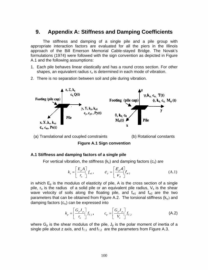
9. Appendix A: Stiffness and Damping Coefficients The stiffness and damping of a single pile and a pile group with

appropriate interaction factors are evaluated for all the piers in the Illinois approach of the Bill Emerson Memorial Cable-stayed Bridge. The Novak’s formulations (1974) were followed with the sign convention as depicted in Figure A.1 and the following assumptions: 1. Each pile behaves linear elastically and has a round cross section. For other

shapes, an equivalent radius r is determined in each mode of vibration. o

2. There is no separation between soil and pile during vibration.

(a) Translational and coupled constraints (b) Rotational constants Figure A.1 Sign convention

A.1 Stiffness and damping factors of a single pile For vertical vibration, the stiffness (kz) and damping factors (cz) are

⎡ ⎤E Ak fp

z w= ⎢ ⎥r 1⎣ ⎦o

⎡E p A ⎤ , c z = ⎢ ⎥fv w 2 (A.1)

⎣ s ⎦

in which Ep is the modulus of elasticity of pile, A is the cross section of a single pile, ro is the radius of a solid pile or an equivalent pile radius, Vs is the shear wave velocity of soils along the floating pile, and fw1 and fw2 are the two parameters that can be obtained from Figure A.2. The torsional stiffness (kψ) and damping factors (cψ) can be expressed into

⎡ ⎤G Jk fp p

ψ = ⎢ ⎥r T ,1⎣ ⎦o

⎡ ⎤G J, c p p

ψ = ⎢ ⎥ fT ,2 (A.2) ⎣ ⎦Vs

where Gp is the shear modulus of the pile, Jp is the polar moment of inertia of a single pile about z axis, and fT,1 and fT,2 are the parameters from Figure A.3.

100

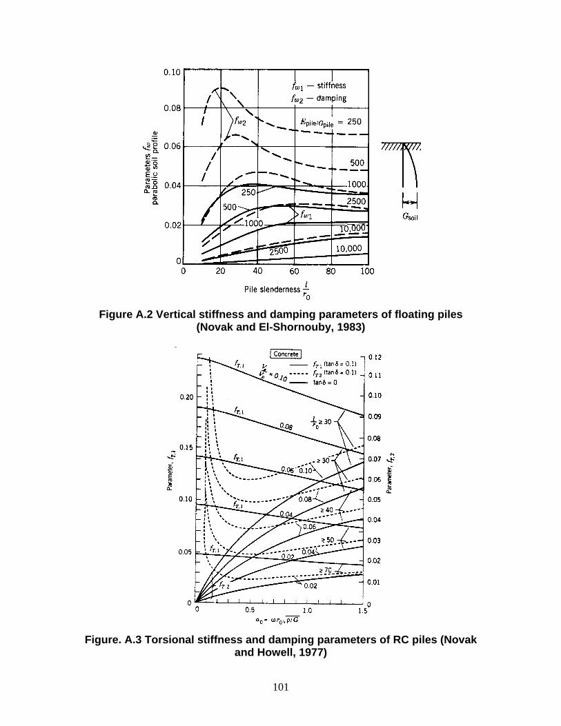
Figure A.2 Vertical stiffness and damping parameters of floating piles

(Novak and El-Shornouby, 1983)

Figure. A.3 Torsional stiffness and damping parameters of RC piles (Novak

and Howell, 1977)

101

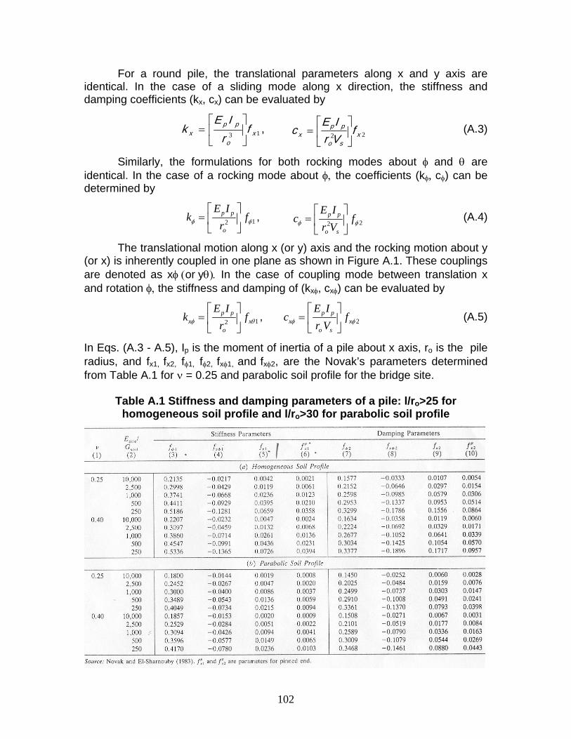
For a round pile, the translational parameters along x and y axis are identical. In the case of a sliding mode along x direction, the stiffness and damping coefficients (kx, cx) can be evaluated by

⎡E p Ik p ⎤

x = ⎢ fr 3 ⎥ x 1 ,

⎣ o ⎦

⎡E pI p ⎤c x = ⎢ f

r 2 ⎥V x 2 (A.3) ⎣ o s ⎦

Similarly, the formulations for both rocking modes about φ and θ are identical. In the case of a rocking mode about φ, the coefficients (kφ, cφ) can be determined by

⎡ ⎤E Ik fp p

φ = ⎢ ⎥r2 φ1 , ⎣ ⎦o

⎡ E Ic = p p ⎤

φ ⎢ r V2 ⎥ fφ 2 (A.4) ⎣ o s ⎦

The translational motion along x (or y) axis and the rocking motion about y (or x) is inherently coupled in one plane as shown in Figure A.1. These couplings are denoted as xφ (or yθ). In the case of coupling mode between translation x and rotation φ, the stiffness and damping of (kxφ, cxφ) can be evaluated by

⎡ ⎤E Ik fp p

xφ = ⎢ ⎥r2 xθ1⎣ ⎦o

⎡ ⎤E I, c fp p

xφ = ⎢ ⎥r V xφ 2 (A.5) ⎣ ⎦o s

In Eqs. (A.3 - A.5), Ip is the moment of inertia of a pile about x axis, ro is the pile radius, and fx1, fx2, fφ1, fφ2, fxφ1, and fxφ2, are the Novak’s parameters determined from Table A.1 for ν = 0.25 and parabolic soil profile for the bridge site.

Table A.1 Stiffness and damping parameters of a pile: l/ro>25 for homogeneous soil profile and l/ro>30 for parabolic soil profile

102

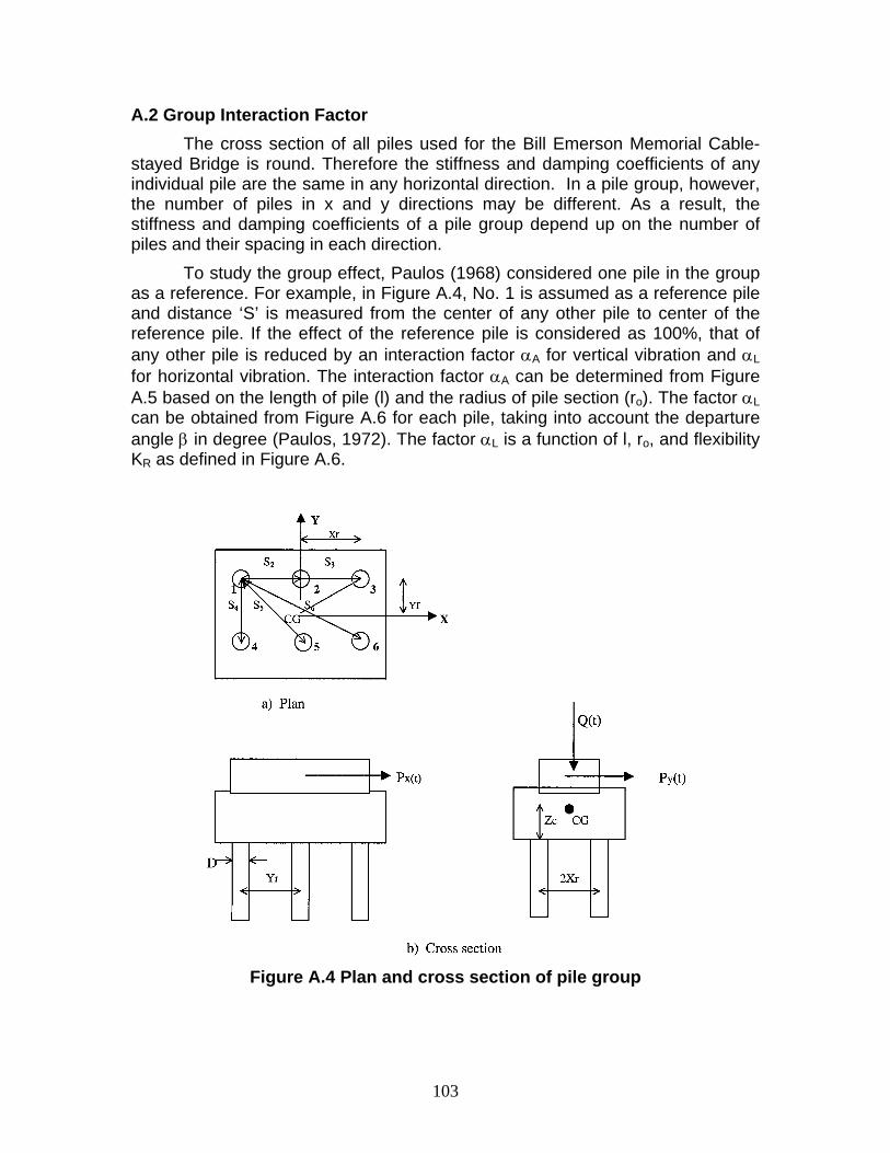
A.2 Group Interaction Factor The cross section of all piles used for the Bill Emerson Memorial Cable-stayed Bridge is round. Therefore the stiffness and damping coefficients of any individual pile are the same in any horizontal direction. In a pile group, however, the number of piles in x and y directions may be different. As a result, the stiffness and damping coefficients of a pile group depend up on the number of piles and their spacing in each direction.

To study the group effect, Paulos (1968) considered one pile in the group as a reference. For example, in Figure A.4, No. 1 is assumed as a reference pile and distance ‘S’ is measured from the center of any other pile to center of the reference pile. If the effect of the reference pile is considered as 100%, that of any other pile is reduced by an interaction factor α for vertical vibration and αA L for horizontal vibration. The interaction factor αA can be determined from Figure A.5 based on the length of pile (l) and the radius of pile section (r ). The factor αo L can be obtained from Figure A.6 for each pile, taking into account the departure angle β in degree (Paulos, 1972). The factor α is a function of l, rL o, and flexibility KR as defined in Figure A.6.

Figure A.4 Plan and cross section of pile group

103

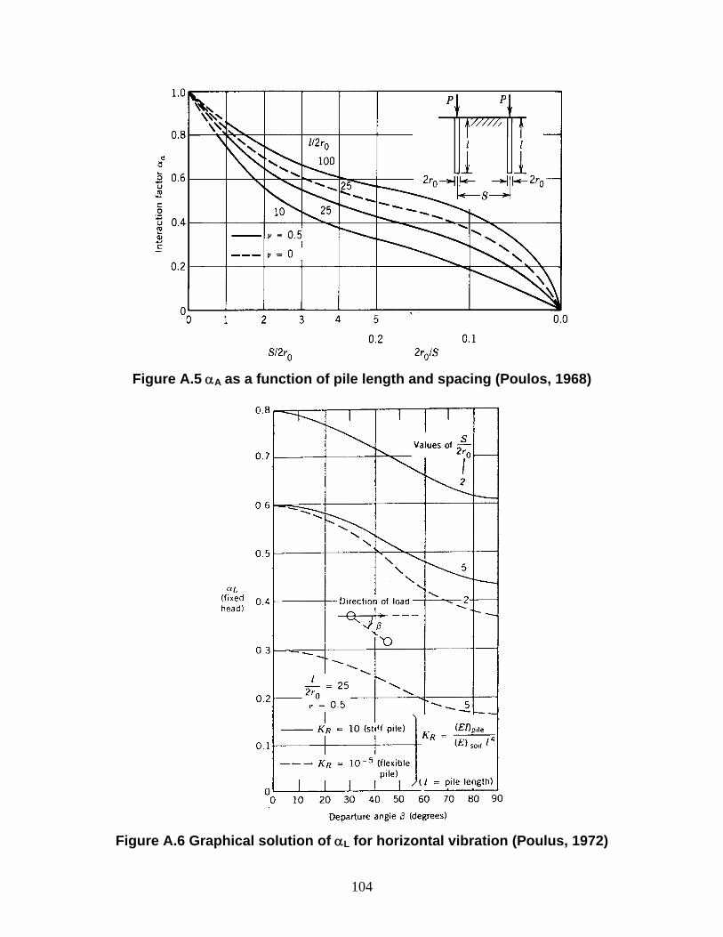
Figure A.5 αA as a function of pile length and spacing (Poulos, 1968)

Figure A.6 Graphical solution of αL for horizontal vibration (Poulus, 1972)

104

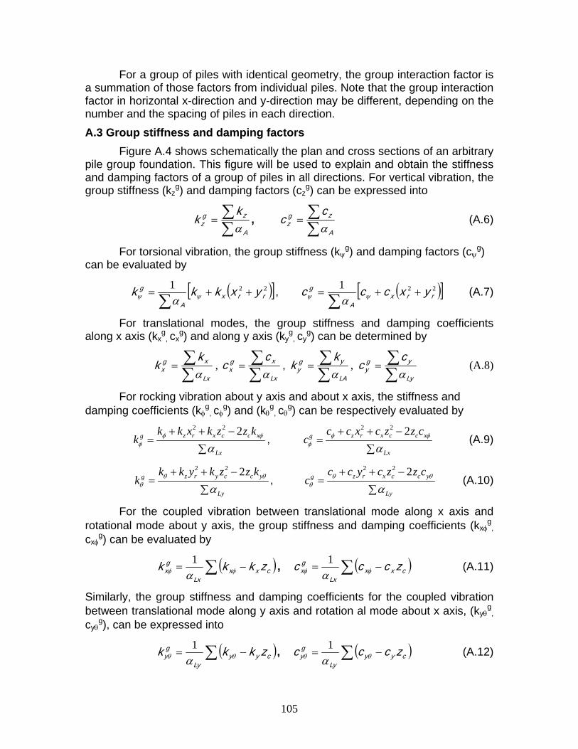
For a group of piles with identical geometry, the group interaction factor is a summation of those factors from individual piles. Note that the group interaction factor in horizontal x-direction and y-direction may be different, depending on the number and the spacing of piles in each direction. A.3 Group stiffness and damping factors

Figure A.4 shows schematically the plan and cross sections of an arbitrary pile group foundation. This figure will be used to explain and obtain the stiffness and damping factors of a group of piles in all directions. For vertical vibration, the group stiffness (k g g) and damping factors (c ) can be expressed into z z

c g = ∑c zz ∑αA

k g = ∑kzz , (

∑A.6)

αA

For torsional vibration, the group stiffness (k gψ ) and damping factors (c g

ψ ) can be evaluated by

k g 1= [ ]k + k ( )2 2

ψ x x r + y∑α ψ r

A

g 1, cψ = [c + ( 2ψ c x x r + y 2

r )] (A.7) ∑αA

For translational modes, the group stiffness and damping coefficients along x axis (k g

x , c gx ) and along y axis (k g

y , c gy ) can be determined by

c g = ∑c xx ∑αLx

k g = ∑kyy ∑αLA

c g = ∑c yy ∑αLy

k g = ∑k xx , , , (A.8)

∑αLx

For rocking vibration about y axis and about x axis, the stiffness and damping coefficients (k g

φ , c gφ ) and (k g

θ , c gθ ) can be respectively evaluated by

k k 2 2g z rx kx zc 2zc xk

k φ + + − φφ =

∑αLx

c c 2 2g z xr cx cz 2zc xc

c φ + + −, φ

φ = (A.9) ∑αLx

k k 2 2g z ry ky zc 2zckk θ + + − yθ

θ =∑αLy

c c+ +2 2g θ z ry cx zc − 2zcc, c yθθ = (A.10)

∑αLy

For the coupled vibration between translational mode along x axis and rotational mode about y axis, the group stiffness and damping coefficients (k g

xφ , c g

xφ ) can be evaluated by

1k gxφ = ∑( )k xφ − k x z

α cLx

, c g 1xφ = ∑( )c xφ − c x zc (A.11)

αLx

Similarly, the group stiffness and damping coefficients for the coupled vibration between translational mode along y axis and rotation al mode about x axis, (k g

yθ , c g

yθ ), can be expressed into

1k gyθ = ∑( )kyθ − ky z

α cLy

1, c gyθ = ∑(c yθ − c y z

α c ) (A.12) Ly

105

10. Appendix B: Unit Conversion

1 m = 3.28 ft 1 cm/sec2 = 0.394 in/sec2

1 km = 0.621 miles 1 kN/m3 = 6.38 lb/ft3

1 kN/m = 68.6 lb/ft 1 kN-m = 0.7371 kip-ft 1 MPa = 0.145 ksi

106

Missouri Department of Transportation Organizational Results P. O. Box 270 Jefferson City, MO 65102

573.526.4335 1 888 ASK MODOT innovation@modot.mo.gov