Oh

HD

a

A

R

R

2

A

K

P

H

C

F

drb

0d

j o u r n a l o f m a t e r i a l s p r o c e s s i n g t e c h n o l o g y 2 0 9 ( 2 0 0 9 ) 1538–1549

journa l homepage: www.e lsev ier .com/ locate / jmatprotec

ptimum shape design of die and preform for improvedardness distribution in cold forged parts

aluk Tumer, Fazıl O. Sonmez ∗

epartment of Mechanical Engineering, Bogazici University, Istanbul, Bebek 34342, Turkiye

r t i c l e i n f o

rticle history:

eceived 12 September 2007

eceived in revised form

4 February 2008

ccepted 4 April 2008

eywords:

rocess optimization

ardness

a b s t r a c t

Hardness of a cold formed part increases due to plastic deformation induced during the

forming process. Hardness affects forgability of the part as well as its mechanical perfor-

mance in use. In this study, a method was proposed to optimize the shape of preform and die

to minimize variation in hardness distribution. The method was applied to backward extru-

sion. A finite element model of the mechanical behavior of the material during processing

was developed to predict the effective strain distribution in the part. The hardness distri-

bution was determined using an analytical relation between effective strain and hardness.

An optimization code based on the Nelder-Mead search algorithm was developed and inte-

grated with the finite element model. The results showed the effectiveness of the proposed

method.

old forging

EM

© 2008 Elsevier B.V. All rights reserved.

ANSYS

1. Introduction

Knowing that hardness is a measure of strength and resis-tance to wear, it should be considered as an important qualityparameter. Accordingly, it highly influences the performanceof products in their service life. High levels of hardness in afinished product may increase its performance for instance inmetal cutting applications but its accompanying low tough-ness makes this part unsuitable for applications requiring highimpact resistance. Uneven hardness distribution is anotherconcern. The regions of high hardness may make the part brit-tle while the regions of low hardness may detract from its wearresistance. In cold forming operations, hardness is not only anoutput of the process and a quality parameter of the end prod-uct, but it is also a parameter that must also be monitored

uring the process. During cold forging of a part, the mate-ial might become so hard that the available press power mayecome unable to deform the workpiece further or the dies

∗ Corresponding author. Tel.: +90 212 359 7196; fax: +90 212 287 2456.E-mail address: sonmezfa@boun.edu.tr (F.O. Sonmez).

924-0136/$ – see front matter © 2008 Elsevier B.V. All rights reserved.oi:10.1016/j.jmatprotec.2008.04.017

and the part itself might be damaged. In order to overcomethis problem, forging operations are usually completed in sub-steps followed by annealing. A cold forming process shouldtherefore be carefully designed so that hardness of the mate-rial during as well as after the processing remains within theacceptable limits.

The change in hardness depends on the permanentdeformation induced during cold forming. By controllingdeformations in a cold forging process, one may control hard-ness and thus achieve a desired level of hardness. For thispurpose, one should know the relationship between defor-mation and hardness for a cold forged part. In that case, if thecontrollable process parameters are related to deformation,one may control deformation, and thus hardness. This means,one may find the values of process parameters resulting in

the desired hardness distribution through an optimizationprocedure.

In the literature, there were a number of studies on opti-mization of cold forging processes. Most of them focused on

t e c h n o l o g y 2 0 9 ( 2 0 0 9 ) 1538–1549 1539

tfipto(atlplbabpicowfcawmaoathraoiTra(mittaimyvbsablafcaa

ogf

Fig. 1 – Die and workpiece geometries (dimensions are in

j o u r n a l o f m a t e r i a l s p r o c e s s i n g

wo major objectives: The first one was to obtain an accuratenal geometry and the second one was to decrease the appliedressure in order to lower the required press capacity, andhus to prevent dies from failures and improve tooling life. Thebjective of the study conducted by Thiyagarajan and Grandhi

2005) was to reduce the difference between the desired andchieved geometries of the finished product and to minimizehe strain variance by optimizing preform shapes in multi-evel forging processes. They defined the boundary curves ofreform shapes by means of coordinates of control points

ying on these boundary curves. They applied the reducedasis technique to decrease the number of optimization vari-bles. Response surface methodology (RSM) was chosen touild an approximation model and perform optimization. Theroposed model was applied on multi-level forging of a steer-

ng link. They reported that a preform shape that enabledomplete die fill was obtained. Zhao et al. (2002) proposed anptimization method for preform shape design. The objectiveas to minimize the effective strain variation in an H-shaped

orging. They defined the preform die shape through B-splineurves. The coordinates of control points were design vari-bles. Broyden–Fletcher–Goldfarb–Shanno (BFGS) algorithmas employed to minimize the objective function. The finalaximum and minimum strains were obtained to be 1.3608

nd 0.350, respectively; they were 1.605 and 0.296 for the non-ptimized case. Although there are similarities between Zhaond Wang’s study and the present study, e.g. FEM is employedo obtain effective strains; our objective is to obtain a uniformardness distribution in a cold forged part, which is directlyelated to the part quality, rather than to minimize the vari-tion in effective strain. Shi et al. (2004) proposed a shapeptimization technique to improve stamping quality by min-

mizing the risk of rupture, wrinkles and unstretched areas.hey utilized the modified sweeping simplex as search algo-ithm. They integrated this algorithm with a FE model andpplied it on a front fender to validate its results. Celano et al.2001) developed a technique for optimum process design of

ulti-pass cold drawing process using the simulated anneal-ng algorithm. The objective of that study was to determinehe optimum number of passes and pass-schedule to keephe drawing stresses on the wire below a safe limit. Theylso showed the effectiveness of their approach by compar-ng it with a set of industrial sequences for wires of different

aterials. Gao and Grandhi (2000) proposed a sensitivity anal-sis based optimization method for improving the grain sizeariation in a forged part. The optimization variables wereillet shape and die velocity. They also set optimization con-traints for die underfill and excessive material waste. Theypplied their method on a turbine disk of waspaloy (a nickelased, age-hardenable super alloy) and obtained optimum bil-

et geometry and die velocity. Roy et al. (1997) carried outcomprehensive study on optimization of multi-stage cold

orming processes. Multi-pass cold wire drawing, multi-passold tubular profile drawing and multi-pass cold forging of anutomotive outer race were the selected processes. They usedmicro genetic algorithm to optimize the process variables.

The literature survey shows that there has been no studyn controlling hardness of cold forged parts by optimizingeometries of preform and die. In this study, a methodologyor optimum process design of cold formed parts was pro-

mm).

posed to obtain uniform hardness distribution. The processto be optimized was chosen to be backward cold extrusion.First, a finite element model of the process was developedin ANSYS environment. This FE model enabled calculationof the effective strains induced in the part during process-ing. Then, the strain–hardness relationship proposed by Demirand Sonmez (2004) and Sonmez and Demir (2007) was used toconvert effective strain values to hardness and thus to deter-mine the hardness distribution. The next step was to developan optimization code based on the Nelder-Mead algorithm(Mathews, 1999). The objective function was defined as thesum of variations in hardness from the average hardness inthe part, and some of the geometric parameters defining dieand preform shapes were chosen as optimization variables. Atlast, the FE model and the optimization code were integrated.Having carried out optimization, the optimum preform anddie shapes were determined.

2. Problem formulation

The backward (cup) extrusion process was considered inthis study because of its prevalence in the industry, highervariation in the strain distribution as a result of highlynonuniform deformation state induced in the workpieceand compatibility to computationally efficient axisymmetricmodeling.

The geometries of the die and workpiece are depicted inFig. 1, while the geometry of the extruded part is shown inFig. 2. The geometries described in these figures were adoptedfrom the study of Hur et al. (2003), in which a design methodfor FE analysis of backward extrusion process was proposed.

The thickness of the walls, the height and depth of the

cup are assumed to be specified according to the require-ments of the product. Since a flat punch tip increases thepress capacity required for inducing the desired deformations,the punch tip is to be curved. The radii of curvatures, R1 and

1540 j o u r n a l o f m a t e r i a l s p r o c e s s i n g t e

Fig. 2 – Geometry of the finished product (dimensions are

The true stress–true strain relation under uniaxial loading

in mm).

R2, defining the tip geometry of the punch are assumed tobe variables for which appropriate values can be chosen dur-ing the process design phase. Only, upper and lower limitsmay be set because of the product requirements during theproduct design phase. The initial shape of the workpiece iscylindrical. In order to place the workpiece inside the die walls,the workpiece diameter should be smaller compared to thatof the die walls. Accordingly, a gap exists between the pre-form and the inner walls of the die. The clearance, t, is tobe determined during the process design phase. R1, R2 and tare therefore considered as independent process optimizationvariables.

Since there may not be a feasible geometry correspond-ing to an arbitrary set of values for the optimization variables,they are not free variables. For this reason, constraints areimposed on the optimization variables considering geomet-ric constraints, design and process requirements, and possibleinstability sources in FE analysis. For fillet radius R1, the mini-mum allowable value is 7.75 mm. which is equal to the radiusof the punch. If both R1 and R2 are chosen to be 7.75 mm, theshape of the punch tip becomes spherical and smaller radiiof curvatures may not be defined. On the other hand, there isno upper limit set for R1. If it tends to go to infinity, the tipbecomes flat.

The upper limit for R2 is 7.75 mm, which is the half of thepunch radius. If R2 takes the value of its upper limit, the curvedefined by R2 eliminates R1, and the punch tip becomes spher-ical. The lower bound of R2 is 3 mm. A lower value may lead todifficulties in FE analysis. This limit was set due to a numberof failed FE analyses below this value.

A very small clearance makes the placement of the pre-form inside the die very difficult. For this reason, a clearanceof 0.1 mm is taken as the lower limit of t. That means theworkpiece should be machined to a diameter being at least0.2 mm smaller than the diameter of the die walls. The upperlimit of t is 0.5 mm. In practice, this limit is too large, sinceit may cause difficulties in workpiece positioning and uncer-

tainties in deformation behavior. The upper limit is taken tobe large, because the feasible domain should be chosen aswide as possible, and should not be restricted based on thecommon practice. Otherwise, one may exclude the globally

c h n o l o g y 2 0 9 ( 2 0 0 9 ) 1538–1549

optimal point from the feasible domain. As will be mentionedlater, the upper limit of 0.5 mm is not active since the optimumvalue of the die gap converges to its lower bound.

3. Hardness–strain relations

Hardness increases with increased amount of deformation.Altan et al. (2005) stated that hardness distribution in coldforged parts could be predicted if the hardness–effective strainrelation of the material and the effective strain distribution inthe finished part were known.

Sonmez and Demir (2007) proposed analytical relationsbetween the effective strain induced in a cold formed work-piece and the resulting Brinell or Vickers hardness. Thisrelation is based on the flow curve constants, which are easilyobtainable.

Vickers hardness (HV) is defined as the load applied on apyramidal indenter divided by the surface area of the perma-nent impression. Since the top angle of a pyramid is 136◦, andits base area is equal to 0.9272 times of its lateral area, HV canbe expressed as

HV = 0.9272Pm (1)

where Pm is the mean pressure (the applied load, F, over theprojected area, A). The base area of the pyramidal impression,A, is calculated by

A = s2

2(2)

where s is the length of the base diagonal. HV is then given by

HV = 0.9272(

2F

s2

)(3)

Consequently, HV can be calculated if the diagonal of theindentation s is measured.

Tabor (1948) assumed that the stress developed at a cer-tain point is representative of the whole deformation and it islinearly related to the average pressure.

Pm = ˛�e (4)

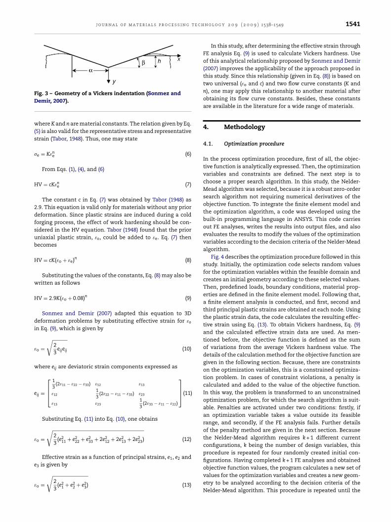
Here, ˛ is a constant and �e is the representative stress.Considering that the indenter used in Vickers hardness

measurements is pyramidal, if the magnitude of the act-ing force is increased, the depth of the impression changeswhereas the impression shape remains unchanged. So theratio h/a (the indentation depth/contact length) remains con-stant regardless of indentation depth (see Fig. 3). That makesε(x/a, y/a) independent of the indentation size. Representativeyield strain εe corresponding to representative yield stress isindependent of the load and hardness, and according to Tabor(1948) it is equal to 0.08.

is described as

� = Kεn (5)

j o u r n a l o f m a t e r i a l s p r o c e s s i n g t e c h

FD

w(s

�

H

2dfsub

H

w

H

di

ε

w

e

ε

e

ε

ig. 3 – Geometry of a Vickers indentation (Sonmez andemir, 2007).

here K and n are material constants. The relation given by Eq.5) is also valid for the representative stress and representativetrain (Tabor, 1948). Thus, one may state

e = Kεne (6)

From Eqs. (1), (4), and (6)

V = cKεne (7)

The constant c in Eq. (7) was obtained by Tabor (1948) as.9. This equation is valid only for materials without any prioreformation. Since plastic strains are induced during a coldorging process, the effect of work hardening should be con-idered in the HV equation. Tabor (1948) found that the priorniaxial plastic strain, εo, could be added to εe. Eq. (7) thenecomes

V = cK(εo + εe)n (8)

Substituting the values of the constants, Eq. (8) may also beritten as follows

V = 2.9K(εo + 0.08)n (9)

Sonmez and Demir (2007) adapted this equation to 3Deformation problems by substituting effective strain for εo

n Eq. (9), which is given by

o =√

23

eijeij (10)

here eij are deviatoric strain components expressed as

ij =

⎡⎢⎣

13

(2ε11 − ε22 − ε33) ε12 ε13

ε1213

(2ε22 − ε11 − ε33) ε23

ε13 ε2313

(2ε33 − ε11 − ε22)

⎤⎥⎦(11)

Substituting Eq. (11) into Eq. (10), one obtains

o =√

23

(e211 + e2

22 + e233 + 2e2

12 + 2e213 + 2e2

23) (12)

Effective strain as a function of principal strains, e1, e2 and

3 is given by

o =√

23

(e21 + e2

2 + e23) (13)

n o l o g y 2 0 9 ( 2 0 0 9 ) 1538–1549 1541

In this study, after determining the effective strain throughFE analysis Eq. (9) is used to calculate Vickers hardness. Useof this analytical relationship proposed by Sonmez and Demir(2007) improves the applicability of the approach proposed inthis study. Since this relationship (given in Eq. (8)) is based ontwo universal (εo and c) and two flow curve constants (K andn), one may apply this relationship to another material afterobtaining its flow curve constants. Besides, these constantsare available in the literature for a wide range of materials.

4. Methodology

4.1. Optimization procedure

In the process optimization procedure, first of all, the objec-tive function is analytically expressed. Then, the optimizationvariables and constraints are defined. The next step is tochoose a proper search algorithm. In this study, the Nelder-Mead algorithm was selected, because it is a robust zero-ordersearch algorithm not requiring numerical derivatives of theobjective function. To integrate the finite element model andthe optimization algorithm, a code was developed using thebuilt-in programming language in ANSYS. This code carriesout FE analyses, writes the results into output files, and alsoevaluates the results to modify the values of the optimizationvariables according to the decision criteria of the Nelder-Meadalgorithm.

Fig. 4 describes the optimization procedure followed in thisstudy. Initially, the optimization code selects random valuesfor the optimization variables within the feasible domain andcreates an initial geometry according to these selected values.Then, predefined loads, boundary conditions, material prop-erties are defined in the finite element model. Following that,a finite element analysis is conducted, and first, second andthird principal plastic strains are obtained at each node. Usingthe plastic strain data, the code calculates the resulting effec-tive strain using Eq. (13). To obtain Vickers hardness, Eq. (9)and the calculated effective strain data are used. As men-tioned before, the objective function is defined as the sumof variations from the average Vickers hardness value. Thedetails of the calculation method for the objective function aregiven in the following section. Because, there are constraintson the optimization variables, this is a constrained optimiza-tion problem. In cases of constraint violations, a penalty iscalculated and added to the value of the objective function.In this way, the problem is transformed to an unconstrainedoptimization problem, for which the search algorithm is suit-able. Penalties are activated under two conditions: firstly, ifan optimization variable takes a value outside its feasiblerange, and secondly, if the FE analysis fails. Further detailsof the penalty method are given in the next section. Becausethe Nelder-Mead algorithm requires k + 1 different currentconfigurations, k being the number of design variables, thisprocedure is repeated for four randomly created initial con-figurations. Having completed k + 1 FE analyses and obtained

objective function values, the program calculates a new set ofvalues for the optimization variables and creates a new geom-etry to be analyzed according to the decision criteria of theNelder-Mead algorithm. This procedure is repeated until the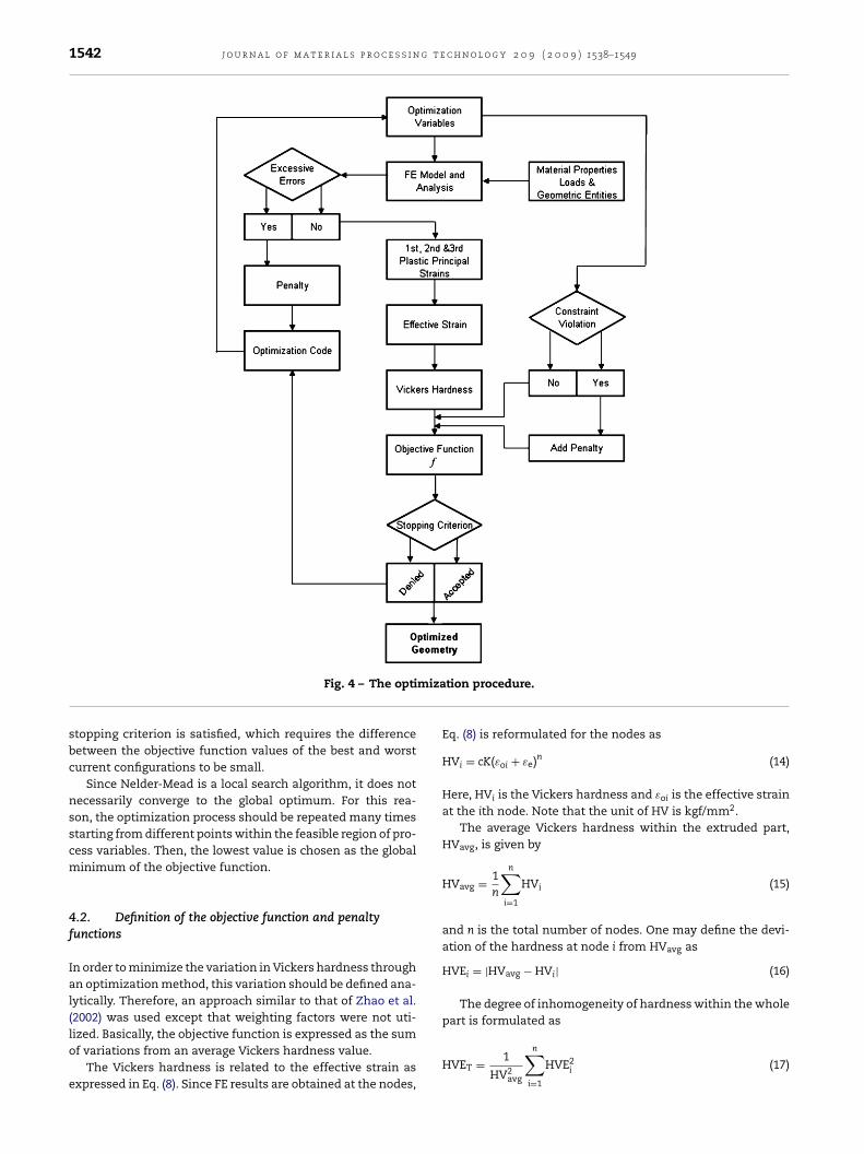

1542 j o u r n a l o f m a t e r i a l s p r o c e s s i n g t e c h n o l o g y 2 0 9 ( 2 0 0 9 ) 1538–1549

miza

Fig. 4 – The opti

stopping criterion is satisfied, which requires the differencebetween the objective function values of the best and worstcurrent configurations to be small.

Since Nelder-Mead is a local search algorithm, it does notnecessarily converge to the global optimum. For this rea-son, the optimization process should be repeated many timesstarting from different points within the feasible region of pro-cess variables. Then, the lowest value is chosen as the globalminimum of the objective function.

4.2. Definition of the objective function and penaltyfunctions

In order to minimize the variation in Vickers hardness throughan optimization method, this variation should be defined ana-lytically. Therefore, an approach similar to that of Zhao et al.(2002) was used except that weighting factors were not uti-

lized. Basically, the objective function is expressed as the sumof variations from an average Vickers hardness value.

The Vickers hardness is related to the effective strain asexpressed in Eq. (8). Since FE results are obtained at the nodes,

tion procedure.

Eq. (8) is reformulated for the nodes as

HVi = cK(εoi + εe)n (14)

Here, HVi is the Vickers hardness and εoi is the effective strainat the ith node. Note that the unit of HV is kgf/mm2.

The average Vickers hardness within the extruded part,HVavg, is given by

HVavg = 1n

n∑i=1

HVi (15)

and n is the total number of nodes. One may define the devi-ation of the hardness at node i from HVavg as

HVEi = |HVavg − HVi| (16)

The degree of inhomogeneity of hardness within the whole

part is formulated as

HVET = 1

HV2avg

n∑i=1

HVE2i (17)

t e c h n o l o g y 2 0 9 ( 2 0 0 9 ) 1538–1549 1543

tf

f

H

fvppfevaaHChpaocb

eofmi

et

x

da

P

a

P

betiNta

s

j o u r n a l o f m a t e r i a l s p r o c e s s i n g

Note that HVET is defined as a power function to intensifyhe effect of deviation in hardness, and it is divided by HV2

avg

or normalization.The objective function, f, is defined as

(R1, R2, t) = w1HVET + w2

l∑k=1

Pk + c� (18)

ere, l is the number of applied penalty functions.During the optimization process, the value of the objective

unction is recalculated whenever the values of optimizationariables are changed by the search algorithm. For this pur-ose, non-linear FE analyses involving large deformation areerformed. The search algorithm may generate a set of valuesor the variables such that for some reason FE analysis fails,.g. the geometry may not be constructed due to a negativealue for the radius of curvature. In that case, effective strainst the nodes, (εoi), cannot be calculated. ANSYS automaticallyssigns zero value for them. According to Eq. (14) and Eq. (15),Vi become equal to the hardness of the starting material.onsequently, the algorithm obtains zero variation in Vickersardness and it sticks to this fake minimum point. In order torevent this, an analysis error term, �, is defined that becomesctive and takes a large value compared to other terms in thebjective function, if FE analysis fails. � is used with a controloefficient c. In such a case, c is equal to 1.0 and the third termecomes nonzero. Otherwise, c is equal to zero.

In Eq. (18), w1 is the weighting constant for HVET and it isqual to 1000, w2 is the weighting coefficient for the penaltiesf constraint violations and it is equal to 10. For all penaltyunctions the same weighting constant is used since all opti-

ization variables have about the same degree of importancen the objective function.

Suppose that for the selected optimization variable, x, therexist a lower and an upper bound denoted by x� and xu, respec-ively. The inequality constraint is expressed as

� < x < xu

This relation requires that two penalty functions beefined. For the lower bound, the penalty function is defineds

k =⟨−x + x�

x�

⟩(19)

nd the penalty function for the upper bound is

k+1 =⟨

x − xu

xu

⟩(20)

Because the type of the penalty functions is external, theyecome active only if their related constraint is violated. Oth-rwise, they are equal to zero. This condition is controlled byhe operator “〈 〉”. If the value of the term inside this operators positive, it yields the same value, otherwise it yields zero.ote that all penalty functions are defined in a manner such

hat they become equal to zero, if their related variable takesvalue within its feasible range.

For R1, there exists only one penalty function since it is con-trained in one direction only whereas two penalty functions

Fig. 5 – FE model with the applied boundary conditions.

are required for both R2 and t, which are constrained in twodirections. Consequently, five penalty functions are employedin the objective function.

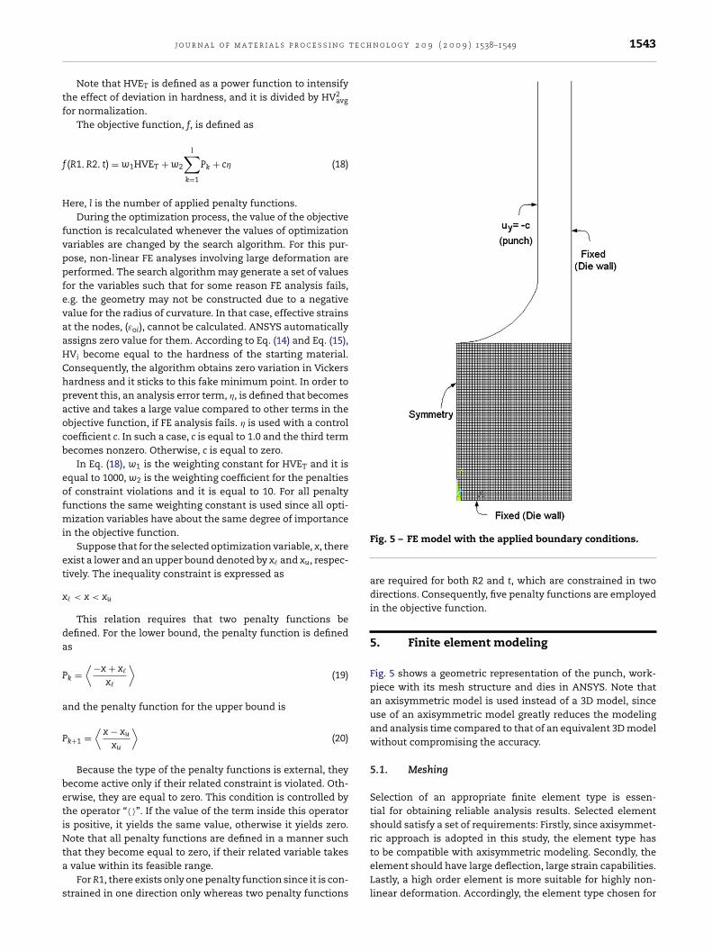
5. Finite element modeling

Fig. 5 shows a geometric representation of the punch, work-piece with its mesh structure and dies in ANSYS. Note thatan axisymmetric model is used instead of a 3D model, sinceuse of an axisymmetric model greatly reduces the modelingand analysis time compared to that of an equivalent 3D modelwithout compromising the accuracy.

5.1. Meshing

Selection of an appropriate finite element type is essen-tial for obtaining reliable analysis results. Selected elementshould satisfy a set of requirements: Firstly, since axisymmet-ric approach is adopted in this study, the element type has

to be compatible with axisymmetric modeling. Secondly, theelement should have large deflection, large strain capabilities.Lastly, a high order element is more suitable for highly non-linear deformation. Accordingly, the element type chosen for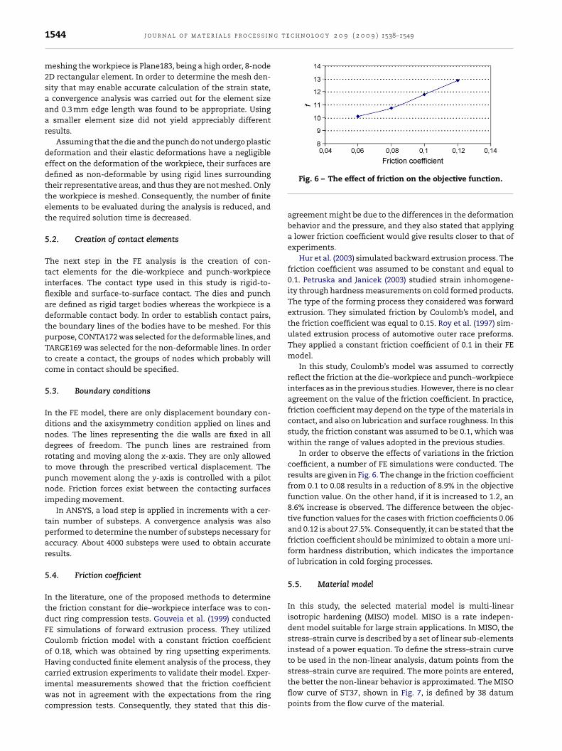

g t e c h n o l o g y 2 0 9 ( 2 0 0 9 ) 1538–1549

1544 j o u r n a l o f m a t e r i a l s p r o c e s s i n

meshing the workpiece is Plane183, being a high order, 8-node2D rectangular element. In order to determine the mesh den-sity that may enable accurate calculation of the strain state,a convergence analysis was carried out for the element sizeand 0.3 mm edge length was found to be appropriate. Usinga smaller element size did not yield appreciably differentresults.

Assuming that the die and the punch do not undergo plasticdeformation and their elastic deformations have a negligibleeffect on the deformation of the workpiece, their surfaces aredefined as non-deformable by using rigid lines surroundingtheir representative areas, and thus they are not meshed. Onlythe workpiece is meshed. Consequently, the number of finiteelements to be evaluated during the analysis is reduced, andthe required solution time is decreased.

5.2. Creation of contact elements

The next step in the FE analysis is the creation of con-tact elements for the die-workpiece and punch-workpieceinterfaces. The contact type used in this study is rigid-to-flexible and surface-to-surface contact. The dies and punchare defined as rigid target bodies whereas the workpiece is adeformable contact body. In order to establish contact pairs,the boundary lines of the bodies have to be meshed. For thispurpose, CONTA172 was selected for the deformable lines, andTARGE169 was selected for the non-deformable lines. In orderto create a contact, the groups of nodes which probably willcome in contact should be specified.

5.3. Boundary conditions

In the FE model, there are only displacement boundary con-ditions and the axisymmetry condition applied on lines andnodes. The lines representing the die walls are fixed in alldegrees of freedom. The punch lines are restrained fromrotating and moving along the x-axis. They are only allowedto move through the prescribed vertical displacement. Thepunch movement along the y-axis is controlled with a pilotnode. Friction forces exist between the contacting surfacesimpeding movement.

In ANSYS, a load step is applied in increments with a cer-tain number of substeps. A convergence analysis was alsoperformed to determine the number of substeps necessary foraccuracy. About 4000 substeps were used to obtain accurateresults.

5.4. Friction coefficient

In the literature, one of the proposed methods to determinethe friction constant for die–workpiece interface was to con-duct ring compression tests. Gouveia et al. (1999) conductedFE simulations of forward extrusion process. They utilizedCoulomb friction model with a constant friction coefficientof 0.18, which was obtained by ring upsetting experiments.Having conducted finite element analysis of the process, they

carried extrusion experiments to validate their model. Exper-imental measurements showed that the friction coefficientwas not in agreement with the expectations from the ringcompression tests. Consequently, they stated that this dis-

Fig. 6 – The effect of friction on the objective function.

agreement might be due to the differences in the deformationbehavior and the pressure, and they also stated that applyinga lower friction coefficient would give results closer to that ofexperiments.

Hur et al. (2003) simulated backward extrusion process. Thefriction coefficient was assumed to be constant and equal to0.1. Petruska and Janicek (2003) studied strain inhomogene-ity through hardness measurements on cold formed products.The type of the forming process they considered was forwardextrusion. They simulated friction by Coulomb’s model, andthe friction coefficient was equal to 0.15. Roy et al. (1997) sim-ulated extrusion process of automotive outer race preforms.They applied a constant friction coefficient of 0.1 in their FEmodel.

In this study, Coulomb’s model was assumed to correctlyreflect the friction at the die–workpiece and punch–workpieceinterfaces as in the previous studies. However, there is no clearagreement on the value of the friction coefficient. In practice,friction coefficient may depend on the type of the materials incontact, and also on lubrication and surface roughness. In thisstudy, the friction constant was assumed to be 0.1, which waswithin the range of values adopted in the previous studies.

In order to observe the effects of variations in the frictioncoefficient, a number of FE simulations were conducted. Theresults are given in Fig. 6. The change in the friction coefficientfrom 0.1 to 0.08 results in a reduction of 8.9% in the objectivefunction value. On the other hand, if it is increased to 1.2, an8.6% increase is observed. The difference between the objec-tive function values for the cases with friction coefficients 0.06and 0.12 is about 27.5%. Consequently, it can be stated that thefriction coefficient should be minimized to obtain a more uni-form hardness distribution, which indicates the importanceof lubrication in cold forging processes.

5.5. Material model

In this study, the selected material model is multi-linearisotropic hardening (MISO) model. MISO is a rate indepen-dent model suitable for large strain applications. In MISO, thestress–strain curve is described by a set of linear sub-elementsinstead of a power equation. To define the stress–strain curveto be used in the non-linear analysis, datum points from the

stress–strain curve are required. The more points are entered,the better the non-linear behavior is approximated. The MISOflow curve of ST37, shown in Fig. 7, is defined by 38 datumpoints from the flow curve of the material.

j o u r n a l o f m a t e r i a l s p r o c e s s i n g t e c h n o l o g y 2 0 9 ( 2 0 0 9 ) 1538–1549 1545

6

6

AActvmmtfirttmtmb

tuu

tid

Table 2 – Starting points and objective function values, f,of the 2nd run and the resulting optimum values

R1 (mm) R2 (mm) t (mm) f

1 85.468 5.075 0.309 14.8742 102.921 4.007 0.235 13.3203 43.702 5.585 0.291 15.5834 85.780 4.140 0.174 13.156

Fig. 7 – MISO flow curve of St37.

. Results and discussions

.1. Initial appraisal of the constraints

fter having developed the optimization code to be run inNSYS environment, a group of optimization iterations wereonducted. Optimization results showed that some variablesend to converge to their either upper or lower limits. If aariable is monotonically increasing to its upper limit, oronotonically decreasing to its lower limit during the opti-ization process, there are two alternatives: one is to extend

he initially chosen feasible domain to search for better con-gurations beyond these limits unless this violates designequirements, process restrictions, and other criteria relatedo computational difficulties. The other alternative is to assignhis limit value to the parameter assuming that this is the opti-

um value for this parameter; it thus becomes a constant inhe following optimization runs. In this way, the global mini-

um can be located more easily and computational cost cane decreased.

Table 1 gives the initial configurations in the first run, andhe resulting optimum values. A second run was conductednder the same conditions with a different set of starting val-es for the variables as given in Table 2.

Note that t and R2 converged to their lower bound in

he first and second runs. For this reason, the correspond-ng constraints and penalty functions are modified as will beiscussed in the following section.

Table 1 – Starting points and objective function values, f,of the first run and the resulting optimum values

R1 (mm) R2 (mm) t (mm) f

1 30.891 5.585 0.291 15.5992 57.974 4.140 0.174 13.1363 15.874 5.059 0.495 15.5584 53.388 4.302 0.386 14.171

Optimum 78.00 3.00 0.11 11.43

Optimum 109.65 3.01 0.12 11.57

In contrast to R2 and t, R1 does not show a tendency to con-verge to its lower bound. Therefore, optimization is continuedwithout any modification on the constraint and correspondingpenalty function of R1.

6.2. Optimum values of the design variables

6.2.1. Die gap tAt the initial phases of the optimization, the smallest allow-able value of t was taken as 0.1 mm. Since t converged toits minimum limit, the feasible range was to extended to0.05 < t < 0.5 mm. However, in this case the preform should bemachined to a higher degree of precision, and this will increasethe manufacturing cost. Using the new lower bound for t, theoptimization process was repeated. As shown in Table 3, tagain converged to its minimum. Note that although R1 and R2converged to the same values (109 mm and 3 mm, respectively)as shown in Tables 2 and 3. The optimum objective functionvalue is smaller for the smaller lower limit. This implies thatchoosing a smaller clearance is conducive to a more uniformhardness distribution.

The lower limit of t was further shifted to 0.01 mm. Thesame initial configurations were used as in the previous case.Only penalty functions were updated according to the newdomain of t. The resulting configuration and the correspond-ing objective function value are given in Table 4. t againconverged to its lower bound, 0.01 mm. One may not choose asmaller clearance, because this requires too tight machiningtolerances for billets unless highly increased machining costscan be tolerated.

One may conclude that the theoretical optimum value of ttends to approach zero. In practice, the optimum value of t isthe tightest tolerance allowed by the manufacturing processused for preparing the workpiece. In this study, t is taken to be

equal to 0.01 mm. From this point on, it becomes a constant,and it is not evaluated in further optimization runs. As a result,the optimization problem is simplified from 3D to 2D.

Table 3 – Starting points and the results for the newfeasible range for t; 0.05 < t < 0.5 mm

R1 (mm) R2 (mm) t (mm) f

1 111.163 5.075 0.309 14.8722 136.835 4.007 0.235 13.3413 56.514 5.585 0.291 15.5744 113.586 4.140 0.174 13.171

Optimum 108.59 3.01 0.05 11.19

1546 j o u r n a l o f m a t e r i a l s p r o c e s s i n g t e

Table 4 – The results for the new feasible range for t;0.01 < t < 0.5 mm

R1 (mm) R2 (mm) t (mm) f

82.392 3.008 0.011 10.868

6.2.2. Corner radius R2Tables 1–4 show that R2 converges to 3.0, as t converges to itsminimum allowed value. Because the value for the lower limitof R2 was chosen in order to avoid difficulties that sharp cor-ners may cause in finite element calculations and also wearingaway of the punch after repeated use, one may assume thatthere is a leeway to relax this constraint also. But first, a newoptimization run was conducted with the die gap t havingfixed to 0.01 mm. Starting points and the resulting optimal val-ues are given in Table 5. It is observed that R2 converges to 3.0as in the previous cases.

After having ensured that the optimum value for R2 doesnot lie close to its maximum boundary, the upper limit wasshifted to 5.0 mm whereas the new lower limit was chosento be 2.0 mm. Another optimization run was conducted usingthese new limits. The corresponding results given in Table 6show that R2 again converges to its lower limit. In this case, thelimits of R2 were revised as 1.5 and 4.0 mm, and the optimiza-tion process was repeated. Table 7 shows that R2 converges to

1.51 mm. This result implies that R2 tends to converge to theminimum possible value allowed by its constraints. On theother hand, too small R2 values may lead to stress concen-tration, shorter tool life and decreased reliability of FE results

Table 5 – Starting points and the results for the case of3.0 < R2 < 7.75

R1 (mm) R2 (mm) f

1 66.822 5.385 13.8202 89.593 5.235 13.5873 136.835 4.007 12.141Optimum 167.80 3.00 10.99

Table 6 – Starting points and the results for the newfeasible range for R2; 2.0 < R2 < 7.75 mm

R1 (mm) R2 (mm) f

1 66.822 4.077 12.1742 89.593 3.854 11.8503 136.835 2.010 9.949

Optimum 137.05 2.00 9.95

Table 7 – Starting points and the results for the newfeasible range for R2; 1.5 < R2 < 4 mm

R1 (mm) R2 (mm) f

1 79.170 2.301 10.2292 128.443 2.955 10.9283 113.586 1.675 9.750

Optimum 36.17 1.51 9.34

c h n o l o g y 2 0 9 ( 2 0 0 9 ) 1538–1549

because of poor convergence. Accordingly, 2.0 mm was con-sidered as a suitable value for R2.

In the following analysis, R2 becomes a constant parame-ter instead of being an optimization variable. Consequently,the only remaining optimization variable is R1. The optimiza-tion problem then becomes a one dimensional problem, whichdecreases the computational effort.

6.2.3. Bottom radius R1Having obtained the optimum values of R2 and t, the remain-ing optimization variable is the punch bottom radius R1.Because the number of design variables is now one (k = 1), thealgorithm uses two (k + 1) current configurations. The resultsof the optimization runs that were carried out to find the opti-mum value of R1 are given in Table 8, which shows that theoptimal value of R1 is between 31.525 and 31.248. In this inter-val, the change in the objective function value is less than0.001. Thus, the optimum value of R1 may be assumed to be31.5 mm.

The values given in Table 9 were selected from the results ofdifferent runs, in which R1 exceeded 100 to show that beyond100 mm, the more R1 is increased, the higher objective func-tion results were obtained. In addition, for the values of R1higher than 200 mm, the curvature on the punch tip becomesnearly flat. Thus, a dramatic change in the objective functionvalues is not expected beyond this limit. One should also notethat the objective function is not very sensitive to changes inR2 when it is large. Thus, if the bottom should be almost flatas a design requirement, the increase in the objective functionwill not be large.

6.3. Evaluation of the results

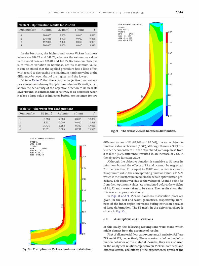
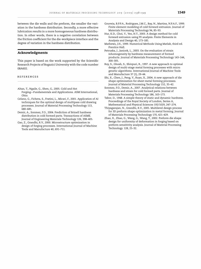
The optimum values of R1, R2, and t were found to be 31.5, 2.0and 0.01 mm, respectively. These values of the optimizationvariables result in an objective function value of 9.573. Theworst four configurations generated by the algorithm duringthe iterations and their resulting objective function values are

given in Table 10. The worst one is 18.007. There is about 46.8%reduction in the variation of the Vickers hardness distribution,which is a dramatic improvement between the worst and thebest case.

Table 8 – Optimization results for R1

Run Initial configurations Final configurations

R1 f R1 f

1113.163 9.868 83.701 9.805

89.593 9.806 86.647 9.805

2101.828 9.836 85.966 9.805136.835 9.899 86.513 9.804

38.257 17.549 31.525 9.573

79.17 9.809 31.248 9.573

479.17 9.809 45.335 9.69556.514 9.795 45.324 9.695

58.0 18.007 31.438 9.573

200.0 9.917 31.25 9.573

j o u r n a l o f m a t e r i a l s p r o c e s s i n g t e c h n o l o g y 2 0 9 ( 2 0 0 9 ) 1538–1549 1547

Table 9 – Optimization results for R1 > 100

Run number R1 (mm) R2 (mm) t (mm) f

1 104.000 2.000 0.010 9.843

viiiwd

usli

2 136.835 2.000 0.010 9.8993 152.000 2.000 0.010 9.9044 200.000 2.000 0.010 9.917

In the best case, the highest and lowest Vickers hardnessalues are 284.73 and 148.75, whereas the extremum valuesn the worst case are 286.81 and 148.95. Because our objectives to reduce variation in hardness, not its maximum value,t can be stated that the applied procedure has a little effect

ith regard to decreasing the maximum hardness value or theifference between that of the highest and the lowest.

Note in Table 10 that the worst two objective function val-

es were obtained using the optimum values of R2 and t, whichhows the sensitivity of the objective function to R1 near itsower bound. In contrast, this sensitivity to R1 decreases whent takes a large value as indicated before. For instance, for two

Table 10 – The worst four configurations

Run number R1 (mm) R2 (mm) t (mm) f

1 8.000 2.000 0.010 18.0072 8.257 2.000 0.010 17.5493 57.774 5.553 0.309 17.0614 30.891 5.585 0.291 15.599

Fig. 8 – The optimum Vickers hardness distribution.

Fig. 9 – The worst Vickers hardness distribution.

different values of R1 (83.701 and 86.647), the same objectivefunction value is obtained (9.805), although there is a 3.5% dif-ference between them. On the other hand, a change in R1 from8 to 8.257 (3.2% difference) resulted in an increase of 2.6% inthe objective function value.

Although the objective function is sensitive to R1 near itsminimum bound, the effects of R2 and t cannot be neglected.For the case that R1 is equal to 30.891 mm, which is close toits optimum value, the corresponding function value is 15.599,which is the fourth worst result in the whole optimization pro-cedure. This result was due to the values of R2 and t being farfrom their optimum values. As mentioned before, the weightsof R1, R2 and t were taken to be same. The results show thatthis was an appropriate choice.

In Figs. 8 and 9, Vickers hardness distribution plots aregiven for the best and worst geometries, respectively. Hard-ness of the inner region increases during extrusion becauseof large deformation. The FE mesh in the deformed shape isshown in Fig. 10.

6.4. Assumptions and discussions

In this study, the following assumptions were made whichmight detract from the accuracy of results:

First of all, material flow curve constants K and n for St37 are

773 and 0.171, respectively. These constants define the defor-mation behavior of the material. Besides, they are also usedin the analytical relationship between Vickers hardness andeffective strain. The effects of the experimental errors or the

1548 j o u r n a l o f m a t e r i a l s p r o c e s s i n g t e

Fig. 10 – The FE mesh in the deformed shape.

errors due to curve fitting were assumed to be negligibly smallon the numerically obtained hardness results.

Secondly, up to 8% error may occur in the predictions of theanalytical Vickers hardness–effective strain relationship givenin Eq. (8) (Sonmez and Demir, 2007). Assuming that the errorsin the lowest and highest predicted hardness values are aboutthe same, the error in the objective function value due to theerror in hardness prediction is expected to be small.

The effect of friction coefficient was high on the resultsas discussed before. In the optimization runs, the FE modelused a constant friction coefficient equal to 0.1. One shouldcorrectly determine the friction coefficient in any real appli-cation.

The initial billet material was assumed to be homogeneousand fully annealed, thus the initial hardness distribution in thebillet was uniform. In addition, the change in hardness of thedeformed workpiece was assumed to be a function of inducedeffective strain, and independent of strain path.

Die and punch surfaces were modeled using rigid lines. In

practice, these surfaces deform elastically, but these deforma-tions are negligible compared to large plastic deformationsinduced in the workpiece. Otherwise, areas representing thedie and the punch would need to be meshed in order to obtain

c h n o l o g y 2 0 9 ( 2 0 0 9 ) 1538–1549

their deformation history, which would highly increase therequired computational capacity.

In this study, optimization variables were mainly con-strained by geometric requirements. One may integratenew constraints and improve effectiveness of the proposedmethodology. Forgability of the product may be monitoredby observing induced stresses in the material. Then, a con-straint may be set for maximum allowable stress above whichinternal cracks develop in the workpiece. In addition, a set ofconstraints may be defined to prevent the die and the punchbeing exposed to stresses higher than their yield strength. Therequired press power may also be obtained, and it may be usedas a constraint related to economic considerations.

The methodology proposed in this thesis is applicableto other types of materials as well as to other cold form-ing processes. If a researcher has the required informationabout the mechanical properties of the material in concernand developed a reliable FE model of the process in con-cern, he/she can adopt the proposed methodology in his/herown study. In addition to different geometric optimizationvariables, different variables and constraints may be definedto enlarge the scope of the proposed method. For instance,stresses developed in the tooling may be constrained to pre-vent tooling failures or improve tooling life. The proposedmethodology may also be adapted to multi-stage cold formingprocesses.

7. Conclusions

In this study, a methodology was proposed to improve thehardness distribution in a backward extruded cup by optimiz-ing preform and die shapes. Two variables defining the punchtip geometry (R1 and R2) and one variable defining the clear-ance between the die and the workpiece (t) were selected asoptimization variables. The objective function was expressedas the sum of variations from the average hardness. Theranges of values that optimization variables could take wereconstrained because of the limitations related to the process,product requirements, and finite element analysis. Penaltyfunctions were utilized in order to account for constraint vio-lations. Nelder-Mead was selected as the search algorithm,since it is a robust zero-order algorithm which makes deci-sions based on the values of the objective function and doesnot require calculation of any derivatives. An optimizationcode was developed using ANSYS parametric design languageincorporating the finite element model and the optimizationprocedure.

The optimum values for the optimization variables R1,R2 and t, were obtained as 31.5, 2.0 and 0.01 mm, respec-tively. The minimum (best) objective function value obtainedduring iterations was 9.573, and the maximum (worst)objective function value was 18.007, which refers to a pos-sible improvement of 46.8% in the objective function incomparison to that of arbitrarily chosen values of designparameters.

In addition to the achieved improvements in the hardnessdistribution, two important design guidelines for an improvedhardness distribution were suggested based on the outputs ofthe optimization procedure. Firstly, the smaller the clearance

t e c h

balttd

A

TR0

r

A

C

D

G

j o u r n a l o f m a t e r i a l s p r o c e s s i n g

etween the die walls and the preform, the smaller the vari-tion in the hardness distribution. Secondly, a more effectiveubrication results in a more homogeneous hardness distribu-ion. In other words, there is a negative correlation betweenhe friction coefficient for the die-workpiece interface and theegree of variation in the hardness distribution.

cknowledgments

his paper is based on the work supported by the Scientificesearch Projects of Bogazici University with the code number8A602.

e f e r e n c e s

ltan, T., Ngaile, G., Shen, G., 2005. Cold and HotForging—Fundamentals and Applications. ASM International,Ohio.

elano, G., Fichera, S., Fratini, L., Micari, F., 2001. Application of AItechniques for the optimal design of multipass cold drawingprocesses. Journal of Material Processing Technology 113,680–685.

emir, A., Sonmez, F.O., 2004. Prediction of Brinell hardness

distribution in cold formed parts. Transactions of ASME.Journal of Engineering Materials Technology 126, 398–405.

ao, Z., Grandhi, R.V., 2000. Microstructure optimization indesign of forging processes. International Journal of MachineTools and Manufacture 40, 691–711.

n o l o g y 2 0 9 ( 2 0 0 9 ) 1538–1549 1549

Gouveia, B.P.P.A., Rodrigues, J.M.C., Bay, N., Martins, N.P.A.F., 1999.Finite element modeling of cold forward extrusion. Journal ofMaterials Processing Technology 94, 85–93.

Hur, K.D., Choi, Y., Yeo, H.T., 2003. A design method for coldforward extrusion using FE analysis. Finite Elements inAnalysis and Design 40, 173–185.

Mathews, J.H., 1999. Numerical Methods Using Matlab, third ed.Prentice Hall.

Petruska, J., Janicek, L., 2003. On the evaluation of straininhomogeneity by hardness measurement of formedproducts. Journal of Materials Processing Technology 143–144,300–305.

Roy, S., Ghosh, S., Shivpuri, R., 1997. A new approach to optimaldesign of multi-stage metal forming processes with microgenetic algorithms. International Journal of Machine Toolsand Manufacture 37 (1), 29–44.

Shi, X., Chen, J., Peng, Y., Ruan, X., 2004. A new approach of dieshape optimization for sheet metal forming processes.Journal of Material Processing Technology 152, 35–42.

Sonmez, F.O., Demir, A., 2007. Analytical relations betweenhardness and strain for cold formed parts. Journal ofMaterials Processing Technology 186, 163–173.

Tabor, D., 1948. A simple theory of static and dynamic hardness.Proceedings of the Royal Society of London, Series A,Mathematical and Physical Sciences 192/1029, 247–274.

Thiyagarajan, N., Grandhi, R.V., 2005. Multilevel design processfor 3D preform shape optimization in metal forming. Journal

of Materials Processing Technology 170, 421–429.

Zhao, X., Zhao, G., Wang, G., Wang, T., 2002. Preform die shapedesign for uniformity of deformation in forging based onpreform sensitivity analysis. Journal of Material ProcessingTechnology. 128, 25–32.