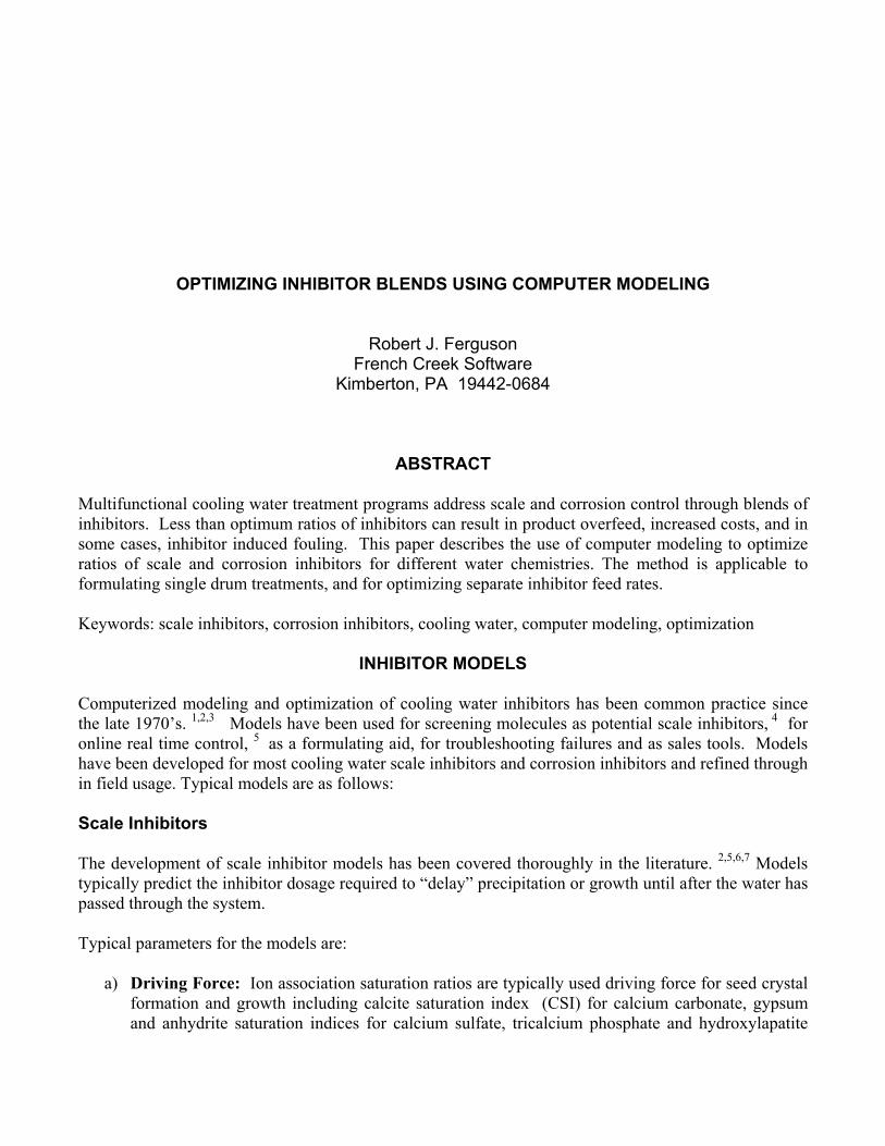
OPTIMIZING INHIBITOR BLENDS USING COMPUTER MODELING

Robert J. Ferguson French Creek Software

Kimberton, PA 19442-0684

ABSTRACT Multifunctional cooling water treatment programs address scale and corrosion control through blends of inhibitors. Less than optimum ratios of inhibitors can result in product overfeed, increased costs, and in some cases, inhibitor induced fouling. This paper describes the use of computer modeling to optimize ratios of scale and corrosion inhibitors for different water chemistries. The method is applicable to formulating single drum treatments, and for optimizing separate inhibitor feed rates. Keywords: scale inhibitors, corrosion inhibitors, cooling water, computer modeling, optimization

INHIBITOR MODELS

Computerized modeling and optimization of cooling water inhibitors has been common practice since the late 1970’s. 1,2,3 Models have been used for screening molecules as potential scale inhibitors, 4 for online real time control, 5 as a formulating aid, for troubleshooting failures and as sales tools. Models have been developed for most cooling water scale inhibitors and corrosion inhibitors and refined through in field usage. Typical models are as follows: Scale Inhibitors The development of scale inhibitor models has been covered thoroughly in the literature. 2,5,6,7 Models typically predict the inhibitor dosage required to “delay” precipitation or growth until after the water has passed through the system. Typical parameters for the models are:

a) Driving Force: Ion association saturation ratios are typically used driving force for seed crystal formation and growth including calcite saturation index (CSI) for calcium carbonate, gypsum and anhydrite saturation indices for calcium sulfate, tricalcium phosphate and hydroxylapatite

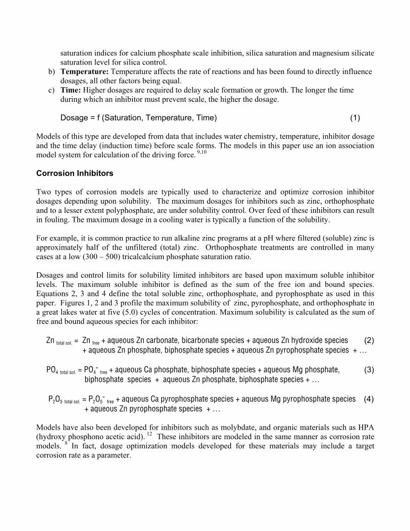
saturation indices for calcium phosphate scale inhibition, silica saturation and magnesium silicate saturation level for silica control.

b) Temperature: Temperature affects the rate of reactions and has been found to directly influence dosages, all other factors being equal.

c) Time: Higher dosages are required to delay scale formation or growth. The longer the time during which an inhibitor must prevent scale, the higher the dosage.

Dosage = f (Saturation, Temperature, Time) (1)

Models of this type are developed from data that includes water chemistry, temperature, inhibitor dosage and the time delay (induction time) before scale forms. The models in this paper use an ion association model system for calculation of the driving force. 9,10 Corrosion Inhibitors Two types of corrosion models are typically used to characterize and optimize corrosion inhibitor dosages depending upon solubility. The maximum dosages for inhibitors such as zinc, orthophosphate and to a lesser extent polyphosphate, are under solubility control. Over feed of these inhibitors can result in fouling. The maximum dosage in a cooling water is typically a function of the solubility. For example, it is common practice to run alkaline zinc programs at a pH where filtered (soluble) zinc is approximately half of the unfiltered (total) zinc. Orthophosphate treatments are controlled in many cases at a low (300 – 500) tricalcalcium phosphate saturation ratio. Dosages and control limits for solubility limited inhibitors are based upon maximum soluble inhibitor levels. The maximum soluble inhibitor is defined as the sum of the free ion and bound species. Equations 2, 3 and 4 define the total soluble zinc, orthophosphate, and pyrophosphate as used in this paper. Figures 1, 2 and 3 profile the maximum solubility of zinc, pyrophosphate, and orthophosphate in a great lakes water at five (5.0) cycles of concentration. Maximum solubility is calculated as the sum of free and bound aqueous species for each inhibitor: Zn total sol. = Zn free + aqueous Zn carbonate, bicarbonate species + aqueous Zn hydroxide species (2) + aqueous Zn phosphate, biphosphate species + aqueous Zn pyrophosphate species + … PO4 total sol. = PO4

= free + aqueous Ca phosphate, biphosphate species + aqueous Mg phosphate, (3) biphosphate species + aqueous Zn phosphate, biphosphate species + …

P2O5 total sol. = P2O5

= free + aqueous Ca pyrophosphate species + aqueous Mg pyrophosphate species (4) + aqueous Zn pyrophosphate species + …

Models have also been developed for inhibitors such as molybdate, and organic materials such as HPA (hydroxy phosphono acetic acid). 12 These inhibitors are modeled in the same manner as corrosion rate models. 8 In fact, dosage optimization models developed for these materials may include a target corrosion rate as a parameter.

Data used to develop these models includes water chemistry, inhibitor level, temperature, and observed corrosion rate. Parameters such as buffer capacity may be calculated from the data and included as parameters in the models. Models can be developed for predicting corrosion rate and for optimizing inhibitor levels.

Corrosion rate = f (water chemistry, inhibitor dosage, temperature) (5)

Inhibitor dosage = f (target corrosion rate, water chemistry, temperature) (6) Figure 4 profiles the dosage requirement for HPA (hydroxy phosphono acetic acid) as a function of target corrosion rate for a great lakes water source at five (5) cycles. Models in this format can be used to compare relative cost options for increasing levels of corrosion control.

OPTIMIZING INHIBITOR BLENDS Water chemistry modeling software has been used effectively to optimize inhibitor ratios using a system similar to this stepwise procedure. In the first example, an alkaline phosphate program is being optimized for a great lakes water at five (5) cycles. Expected maximum water temperature is 130 oF. The product is being formulated for treatment at 100 ppm (as product) in the recirculating water. Inhibitors used in the desired formulation include:

• PBTC (2-Phosphonobutane 1,2,4-tricarboxylic acid) for calcium carbonate scale control; • A Copolymer (copolymer of acrylic acid and 2-Acrylamido-2-Methylpropyl Sulfonic Acid) for calcium

phosphate scale control; and • Orthophosphate as a corrosion inhibitor.

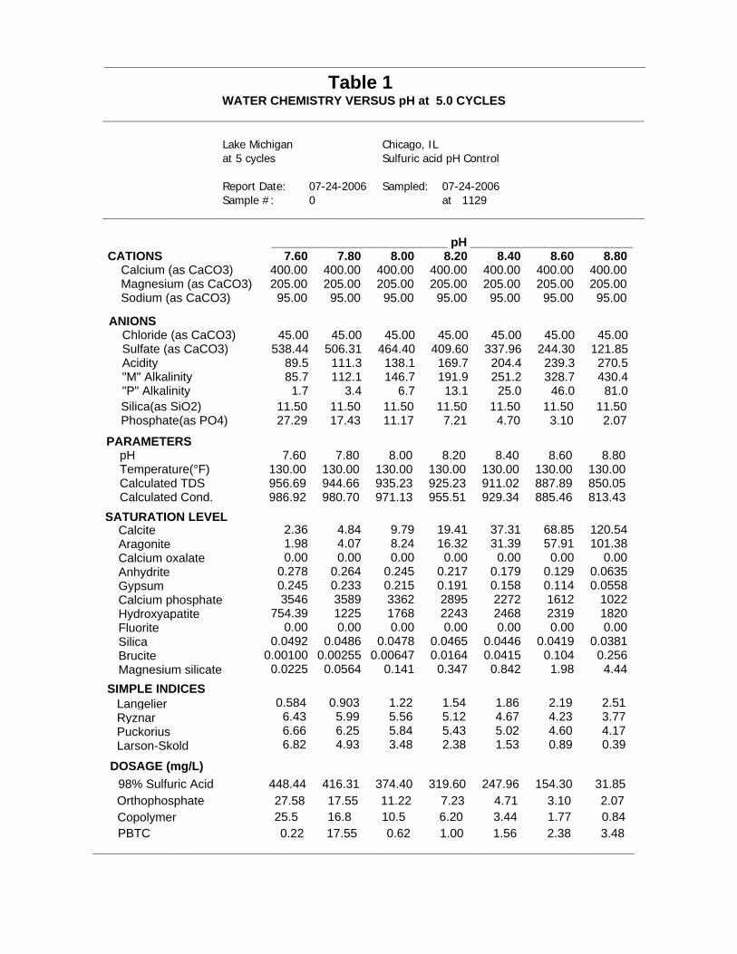
Step 1: Confirm Water Chemistry and Problems. The first step in optimizing an inhibitor blend is to model its properties at the target concentration ratio and operating range. Once the water is concentrated by the computer, predict the scales that must be controlled and the expected mild steel corrosion rate without treatment. These factors will usually be known based upon experience with the water under study. Figure 5 models a Lake Michigan water at Chicago, Il, at five (5.0) cycles of concentration. Predicted corrosion rates are for an untreated system. Table 1 summarizes the scales and predicted corrosion rate for the water as it cycles. Step 2: Determine Corrosion Inhibitor Requirement (orthophosphate). Select the corrosion inhibitor to be optimized. Many corrosion inhibitors are potential foulants, so the expected level in the recirculating water must be known so that adequate stabilization agents can be added to control potential deposits from the inhibitor. Figure 6 depicts the computer model orthophosphate dosage in the target operating range. Step 3: Determine Calcium phosphate Inhibitor Requirement. (copolymer) Set background phosphate to desired orthophosphate level in the recirculating water. Use a model for the calcium phosphate inhibitor to determine the calcium phosphate inhibitor requirements. Figure 7 depicts the copolymer requirement as recommended by the computer model.

Step 4: Determine Calcium carbonate Inhibitor Requirement. (PBTC) Select a model for the calcium carbonate inhibitor to determine the PBTC requirements. Figure 8 depicts the PBTC requirement as recommended by the computer model. For treatments with separate feed of scale and corrosion inhibitors, dosages have been determined. If formulating a “one drum” treatment approach, proceed to step 5. Step 5: Calculate the Product Formulation The computer models used are based upon active inhibitor levels. The active levels and calculated formulation percentages are highlighted in Table 2. Please note that the calculated ratios are optimized for in use concentrations and may not be stable at formulation percentages in a single drum approach. The art of formulation must be practiced to develop stable formulations with the required ratios. Step 6: Verify blend The modeling software used for this report checks to assure that sufficient polymer is present to control any calcium phosphate scale potential created by the treatment. First the program calculates the phosphate level required under the conditions evaluated. Then the program calculates the treated water calcium phosphate scale potential , and the polymer requirement to control it. If sufficient polymer is present, greater to or equal to that recommended for the orthophosphate present, the program proceeds without warning. If the program finds insufficient polymer present, it warns that the polymer to phosphate ratio is too low, either by color coding graphs magenta, or by enclosing dosages in brackets. Figure 9 profiles the treatment requirement for the product formulated. Note that the product was formulated to handle a pH of 8.0 at 130oF. The shaded values in Table 2 were used for formulation.

OTHER ALKALINE PHOSPHATE TREATMENT SCHEMES

The scenario evaluated is for a high phosphate treatment approach, which is applicable to high flow velocity systems. Modeling software has been used successfully to optimize two other scenarios as well. Other calcium carbonate scale inhibitors, such as HEDP (1,1 – hydroxy ethylidene dihposphonic acid) are also included in many alkaline treatment approaches and can be included in optimization models. Low Phosphate Approach Early alkaline phosphate treatment programs operated on the razor edge of calcium phosphate scale solubility. Phosphate levels were controlled near or slightly above the maximum soluble orthophosphate level. Low levels of polymer were introduced into the formulations with the goal of controlling scale at a level low enough so that the scale control agent present would not interfere with inhibitor film formation. Control levels for a low phosphate approach are outlined in Table 3. The phosphate levels recommended follow from Figure 3.

Moderate Tricalcium phosphate Approach Alkaline phosphate treatment programs in large volume heavy industrial systems are operated in many cases at a moderate degree of calcium phosphate supersaturation. Phosphate levels are controlled so that the water has a tricalcium phosphate (TCP) saturation level on the close order of 500x saturation. Moderate levels of polymer are required in these formulations to prevent scale formation in low flow velocity exchangers. Control levels for a Moderate TCP approach are outlined in Table 4. Other Treatment Approaches Computer modeling has been used successfully for modeling multifunctional treatment programs based upon other combinations of inhibitors such as organic phosphate (e.g. PCA - phosphono carboxylic acid, HPA, phosphonates), zinc, polyphosphate, and orthophosphate. Models have been used to optimize treatment programs with separate feeds of scale inhibitors, stabilizers, and corrosion inhibitors, and for optimizing inhibitor blends in a single formulation. In all cases, the models are used to balance corrosion inhibitor level and performance with scale control agent dosage.

SUMMARY Computer modeling provides insight into the application, operation and formulation of multifunctional inhibitor blends. Models can be used to optimize formulations and assure that sufficient scale control agent levels are present to control any fouling potential created by the treatment (e.g. Zn, PO4), while limiting costly overfeed. In the case of fixed ratio formulations, evaluations of a treatment scheme also provides insight into the limitations with respect to the pH and temperature due to the ratio of scale control agent to potential scale forming corrosion inhibitors being applied. Computer modeling is not a panacea. It requires reasonable models for scale and corrosion inhibitors as well as knowledge of the target cooling system operating range.

REFERENCES 1. C. J. Schell, The Use of Computer Modeling in Calguard to Mathematically Simulate Cooling Water

Systems and Retrieve Data, International Water Conference, 41st Annual Meeting, Pittsburgh, Pennsylvania, IWC-80-43 (1980).

2. D. A. Johnson, K. E. Fulks, Computerized Water Modeling in the Design and Operation of Industrial

Cooling Systems, International Water Conference, 41st Annual Meeting, Pittsburgh, Pennsylvania, IWC-80-42 (1980).

3. R. J. Ferguson, "Developing Scale Inhibitor Dosage Models," Proceedings of WaterTech ‘92,

Houston, TX. (1992).

4. P. J. Sullivan, F. O'Brien, R. J. Ferguson, “A Multifunctional Additive for Deposit Control,” CORROSION 96, Paper No. 96158, NACE International (1996).

5. R. J. Ferguson, O. Codina, W. Rule, R. Baebel, Real Time Control of Scale Inhibitor Feed Rate, International Water Conference, 49th Annual Meeting, Pittsburgh, Pennsylvania, IWC-88-57 (1988).

6. R. J. Ferguson, "Thirty Years of Ultra Low Dosage Scale Control," CORROSION 03, Paper No. 03063, NACE International (2003).

7. B. W. Ferguson, R. J. Ferguson, “Sidestream Evaluation of Fouling Factors in a Utility Surface Condenser,” Journal of the Cooling Tower Institute, p. 31-39 (1981).

8. R. J. Ferguson, "Developing Corrosion Inhibitor Models," Proceedings of WaterTech ‘93, Houston, TX. (1993).

9. R. J. Ferguson, A. J. Freedman, G. Fowler, A. J. Kulik, J. Robson, D. J. Weintritt, “The Practical Application of Ion Association Model Saturation Level Indices To Commercial Water Treatment Problem Solving,” (Washington, DC: American Chemical Society Annual Meeting, Division of Colloid and Surface Chemistry Symposia, Scale Formation and Inhibition, 1994).

10. R. J. Ferguson, Computerized Ion Association Model Profiles Complete Range of Cooling System Parameters, International Water Conference, 52nd Annual Meeting, Pittsburgh, PA, IWC-91-47 (1991).

11. WaterCycle®, French Creek Software

12. BWA Belcor® 575

________________________________________________________________________________

Table 1 WATER CHEMISTRY VERSUS pH at 5.0 CYCLES

________________________________________________________________________________

Lake Michigan Chicago, ILat 5 cycles Sulfuric acid pH Control

Report Date: 07-24-2006 Sampled: 07-24-2006Sample #: 0 at 1129

________________________________________________________________________________

__________________________ pH ________________________CATIONS 7.60 7.80 8.00 8.20 8.40 8.60 8.80

Calcium (as CaCO3) 400.00 400.00 400.00 400.00 400.00 400.00 400.00Magnesium (as CaCO3) 205.00 205.00 205.00 205.00 205.00 205.00 205.00Sodium (as CaCO3) 95.00 95.00 95.00 95.00 95.00 95.00 95.00

ANIONSChloride (as CaCO3) 45.00 45.00 45.00 45.00 45.00 45.00 45.00Sulfate (as CaCO3) 538.44 506.31 464.40 409.60 337.96 244.30 121.85Acidity 89.5 111.3 138.1 169.7 204.4 239.3 270.5"M" Alkalinity 85.7 112.1 146.7 191.9 251.2 328.7 430.4"P" Alkalinity 1.7 3.4 6.7 13.1 25.0 46.0 81.0Silica(as SiO2) 11.50 11.50 11.50 11.50 11.50 11.50 11.50Phosphate(as PO4) 27.29 17.43 11.17 7.21 4.70 3.10 2.07

PARAMETERSpH 7.60 7.80 8.00 8.20 8.40 8.60 8.80Temperature(°F) 130.00 130.00 130.00 130.00 130.00 130.00 130.00Calculated TDS 956.69 944.66 935.23 925.23 911.02 887.89 850.05Calculated Cond. 986.92 980.70 971.13 955.51 929.34 885.46 813.43

98% Sulfuric Acid 448.44 416.31 374.40 319.60 247.96 154.30 31.85DOSAGE (mg/L)

Orthophosphate 27.58 17.55 11.22 7.23 4.71 3.10 2.07

________________________________________________________________________________

Copolymer 25.5 16.8 10.5 6.20 3.44 1.77 0.84PBTC 0.22 17.55 0.62 1.00 1.56 2.38 3.48

Calcite 2.36 4.84 9.79 19.41 37.31 68.85 120.54Aragonite 1.98 4.07 8.24 16.32 31.39 57.91 101.38Calcium oxalate 0.00 0.00 0.00 0.00 0.00 0.00 0.00Anhydrite 0.278 0.264 0.245 0.217 0.179 0.129 0.0635Gypsum 0.245 0.233 0.215 0.191 0.158 0.114 0.0558Calcium phosphate 3546 3589 3362 2895 2272 1612 1022Hydroxyapatite 754.39 1225 1768 2243 2468 2319 1820Fluorite 0.00 0.00 0.00 0.00 0.00 0.00 0.00Silica 0.0492 0.0486 0.0478 0.0465 0.0446 0.0419 0.0381Brucite 0.00100 0.00255 0.00647 0.0164 0.0415 0.104 0.256Magnesium silicate 0.0225 0.0564 0.141 0.347 0.842 1.98 4.44

SATURATION LEVEL

SIMPLE INDICESLangelier 0.584 0.903 1.22 1.54 1.86 2.19 2.51Ryznar 6.43 5.99 5.56 5.12 4.67 4.23 3.77Puckorius 6.66 6.25 5.84 5.43 5.02 4.60 4.17Larson-Skold 6.82 4.93 3.48 2.38 1.53 0.89 0.39

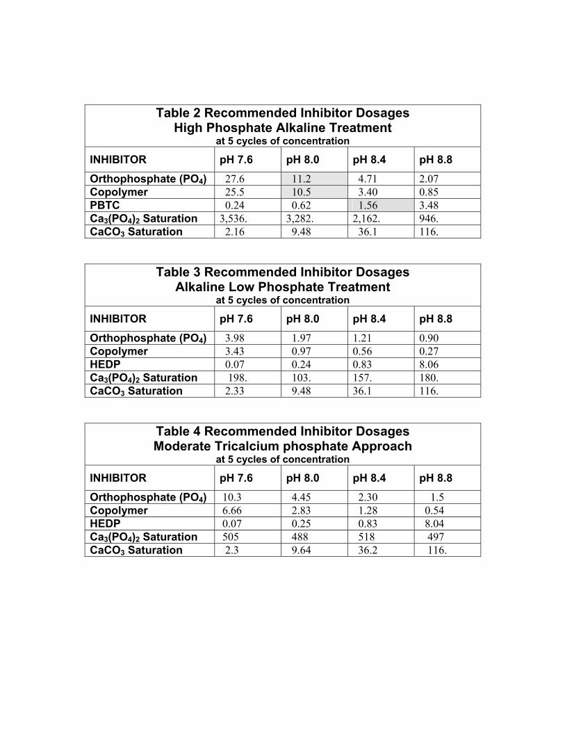
Table 2 Recommended Inhibitor Dosages High Phosphate Alkaline Treatment

at 5 cycles of concentration

INHIBITOR pH 7.6 pH 8.0 pH 8.4 pH 8.8

Orthophosphate (PO4) 27.6 11.2 4.71 2.07 Copolymer 25.5 10.5 3.40 0.85 PBTC 0.24 0.62 1.56 3.48 Ca3(PO4)2 Saturation 3,536. 3,282. 2,162. 946. CaCO3 Saturation 2.16 9.48 36.1 116.

Table 3 Recommended Inhibitor Dosages Alkaline Low Phosphate Treatment

at 5 cycles of concentration

INHIBITOR pH 7.6 pH 8.0 pH 8.4 pH 8.8

Orthophosphate (PO4) 3.98 1.97 1.21 0.90 Copolymer 3.43 0.97 0.56 0.27 HEDP 0.07 0.24 0.83 8.06 Ca3(PO4)2 Saturation 198. 103. 157. 180. CaCO3 Saturation 2.33 9.48 36.1 116.

Table 4 Recommended Inhibitor Dosages Moderate Tricalcium phosphate Approach

at 5 cycles of concentration

INHIBITOR pH 7.6 pH 8.0 pH 8.4 pH 8.8

Orthophosphate (PO4) 10.3 4.45 2.30 1.5 Copolymer 6.66 2.83 1.28 0.54 HEDP 0.07 0.25 0.83 8.04 Ca3(PO4)2 Saturation 505 488 518 497 CaCO3 Saturation 2.3 9.64 36.2 116.

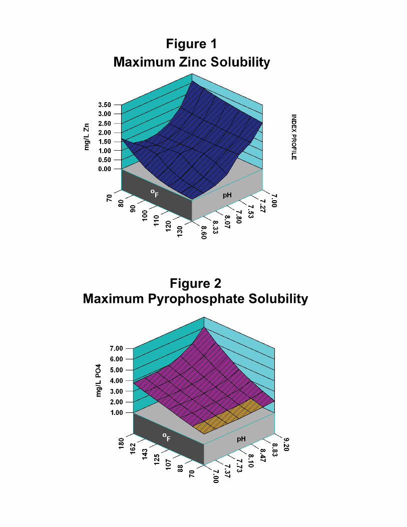
Figure 1

Figure 2 Maximum Pyrophosphate Solubility

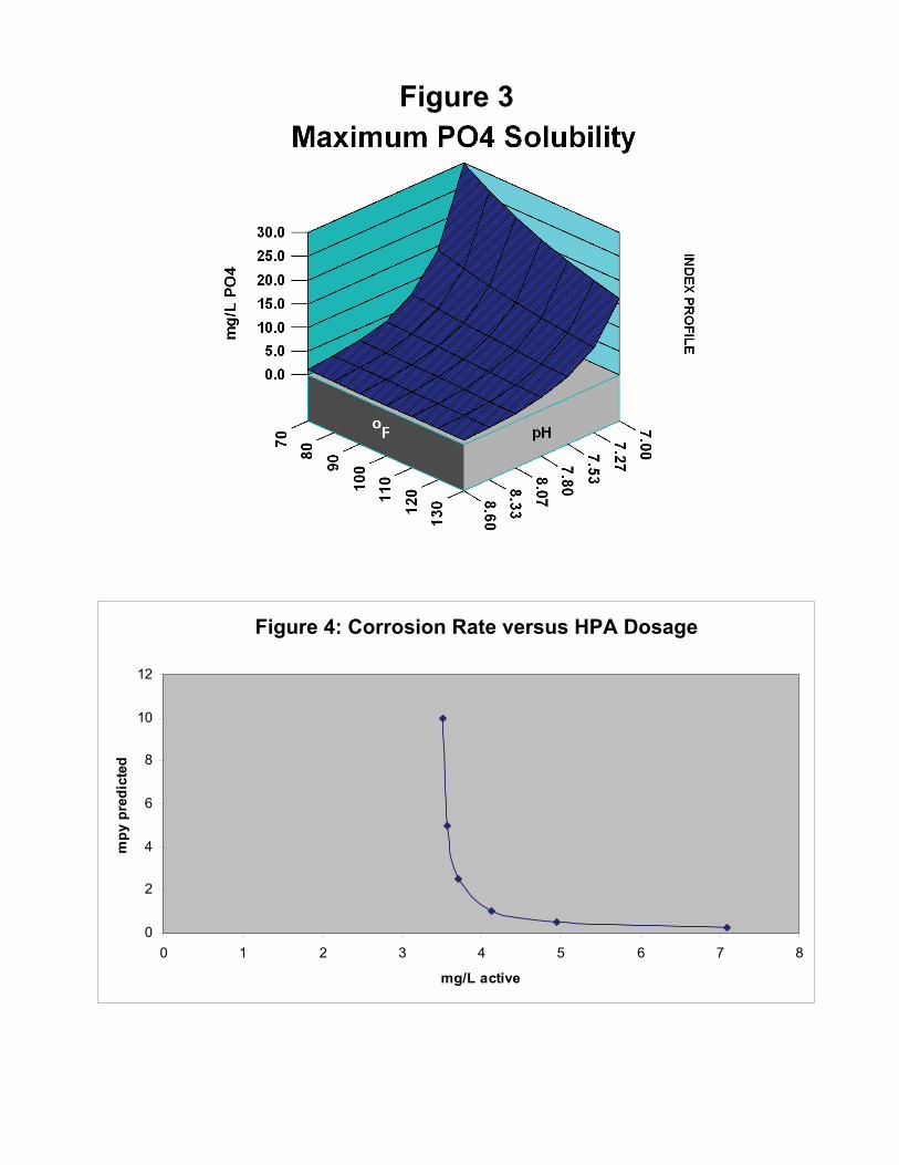
Figure 3

Figure 4: Corrosion Rate vs PCA Dosage

0

2

4

6

8

10

12

0 1 2 3 4 5 6 7 8

mg/L active

mpy

pre

dict

ed

Figure 4: Corrosion Rate versus HPA Dosage

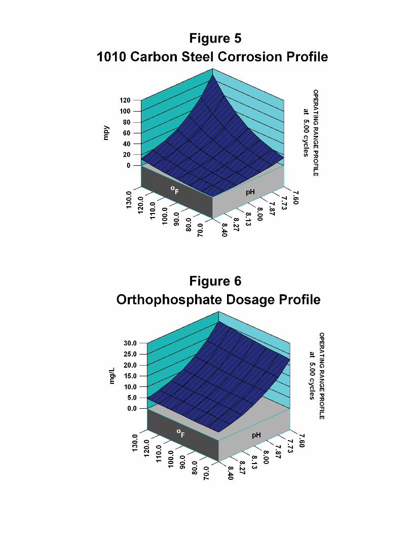
Figure 5

Figure 6

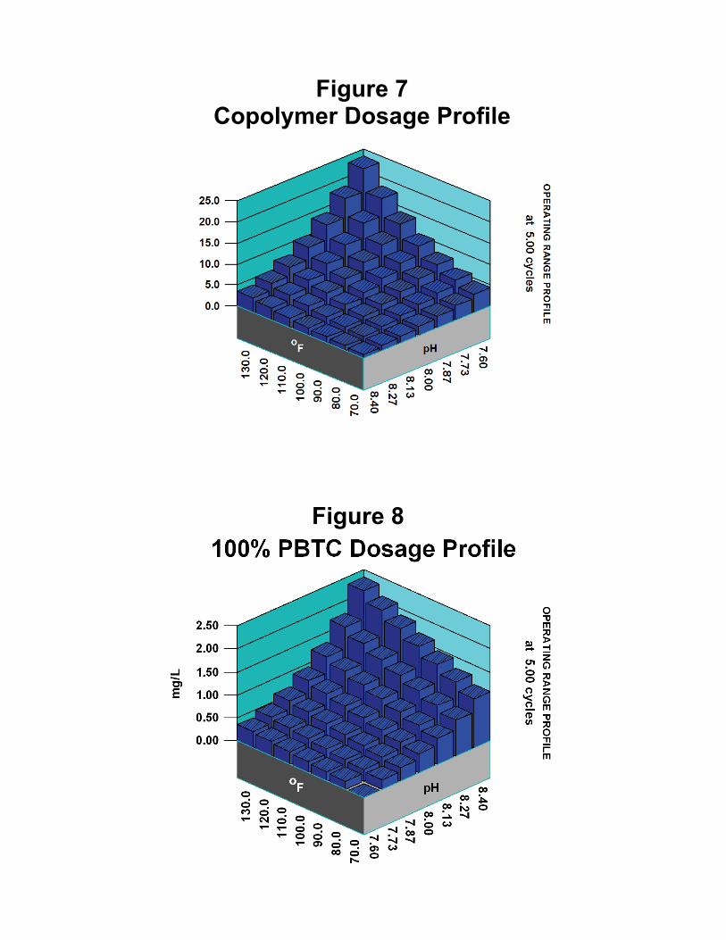
Figure 7 Copolymer Dosage Profile

Figure 8

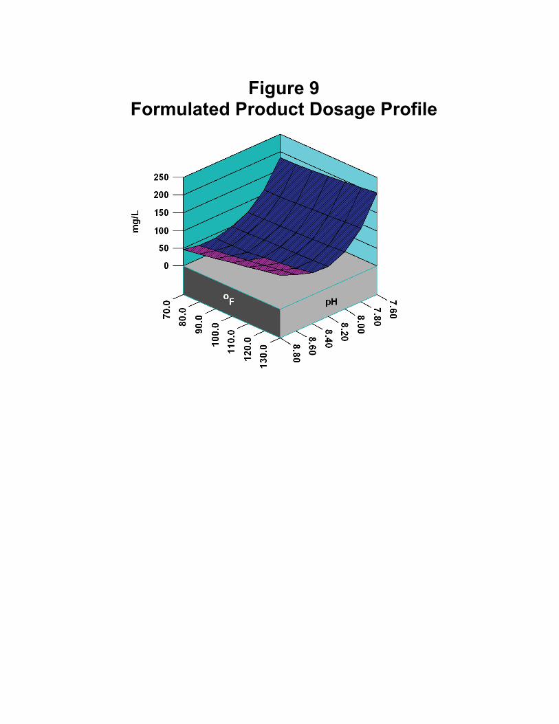
Figure 9 Figure 9 Formulated Product Dosage Profile