Abstract Drylands occupy ∼40% of the land surface and are thought to dominate global carbon (C) cycle inter-annual variability (IAV). Therefore, it is imperative that global terrestrial biosphere models (TBMs), which form the land component of IPCC earth system models, are able to accurately simulate dryland vegetation and biogeochemical processes. However, compared to more mesic ecosystems, TBMs have not been widely tested or optimized using in situ dryland CO2 fluxes. Here, we address this gap using a Bayesian data assimilation system and 89 site-years of daily net ecosystem exchange (NEE) data from 12 southwest US Ameriflux sites to optimize the C cycle parameters of the ORCHIDEE TBM. The sites span high elevation forest ecosystems, which are a mean sink of C, and low elevation shrub and grass ecosystems that are either a mean C sink or “pivot” between an annual C sink and source. We find that using the default (prior) model parameters drastically underestimates both the mean annual NEE at the forested mean C sink sites and the NEE IAV across all sites. Our analysis demonstrated that optimizing phenology parameters are particularly useful in improving the model's ability to capture both the magnitude and sign of the NEE IAV. At the forest sites, optimizing C allocation, respiration, and biomass and soil C turnover parameters reduces the underestimate in simulated mean annual NEE. Our study demonstrates that all TBMs need to be calibrated for dryland ecosystems before they are used to determine dryland contributions to global C cycle variability and long-term carbon-climate feedbacks.

Plain Language Summary Drylands occupy ∼40% of the land surface and are thought to dominate the inter-annual variability and long-term trend of the global carbon cycle. Therefore, it is imperative that global terrestrial biosphere models (TBMs) are able to accurately predict dryland vegetation and carbon cycle processes. However, models have not been widely tested or calibrated against in situ dryland ecosystem CO2 fluxes. Here, we address this gap using a data assimilation system and daily net CO2 flux data from 12 southwest US Ameriflux sites spanning forest, shrub and grass dryland ecosystems to optimize the carbon cycle related parameters of the ORCHIDEE TBM. We find that before parameter optimization, the model drastically underestimates both the mean annual magnitude and inter-annual variability of net CO2 flux. By testing different optimization scenarios, we showed that optimizing model parameters related to phenology dramatically improves the model's ability to capture the net CO2 flux inter-annual variability. At the high elevation forested sites, optimizing parameters related to C allocation, respiration and biomass and soil C turnover reduces the model underestimate in simulated mean annual NEE. Our study demonstrates that all global TBMs need to be calibrated specifically for dryland ecosystems before they are used to determine dryland contributions to global carbon cycle variability and long-term carbon-climate feedbacks.

MAHMUD ET AL.

© 2021. American Geophysical Union. All Rights Reserved.

Optimizing Carbon Cycle Parameters Drastically Improves Terrestrial Biosphere Model Underestimates of Dryland Mean Net CO2 Flux and its Inter-Annual VariabilityKashif Mahmud1 , Russell L. Scott2 , Joel A. Biederman2 , Marcy E. Litvak3 , Thomas Kolb4 , Tilden P. Meyers5, Praveena Krishnan5,6 , Vladislav Bastrikov7,8 , and Natasha MacBean1

1Department of Geography, Indiana University, Bloomington, IN, USA, 2Southwest Watershed Research Center, United States Department of Agriculture, Agricultural Research Service, Tucson, AZ, USA, 3Department of Biology, University of New Mexico, Albuquerque, NM, USA, 4School of Forestry, Northern Arizona University, Flagstaff, AZ, USA, 5NOAA/ARL Atmospheric Turbulence and Diffusion Division, Oak Ridge, TN, USA, 6Oak Ridge Associated Universities, Oak Ridge, TN, USA, 7Laboratoire des Sciences du Climat et de l’Environnement, LSCE/IPSL, CEA-CNRS-UVSQ, Université Paris-Saclay, Gif-sur-Yvette, France, 8Now at Science Partners, Paris, France

Key Points:• ORCHIDEE terrestrial biosphere

model radically underestimates dryland mean annual net CO2 fluxes and their inter-annual variability (IAV)

• Optimizing phenology, carbon allocation, and respiration parameters are crucial for capturing net CO2 flux mean and IAV

• Models need to be optimized against dryland CO2 flux data to achieve accurate predictions of dryland's role in global C cycle variability

Supporting Information:Supporting Information may be found in the online version of this article.

Correspondence to:K. Mahmud,kmahmud@iu.edu

Citation:Mahmud, K., Scott, R. L., Biederman, J. A., Litvak, M. E., Kolb, T., Meyers, T. P., et al. (2021). Optimizing carbon cycle parameters drastically improves terrestrial biosphere model underestimates of dryland mean net CO2 flux and its inter-annual variability. Journal of Geophysical Research: Biogeosciences, 126, e2021JG006400. https://doi.org/10.1029/2021JG006400

Received 6 MAY 2021Accepted 29 SEP 2021

10.1029/2021JG006400RESEARCH ARTICLE

1 of 23

Journal of Geophysical Research: Biogeosciences

MAHMUD ET AL.

10.1029/2021JG006400

2 of 23

1. IntroductionTerrestrial ecosystems currently take up ∼30% of anthropogenic CO2 emissions, thus acting as a substantial global carbon (C) sink (Fu et al., 2017) and providing a critical reduction in the rate of global warming. However, while we know the magnitude of the global C sink to a good degree of certainty, our knowledge of other components of the global C cycle are more uncertain. One such knowledge gap is which ecosystems, and/or which processes, are driving inter-annual variability (IAV) in land net C uptake (Fu et al., 2017). Improving our understanding of the IAV characteristics of the global terrestrial C cycle is key to being able to forecast the future of the land C sink and long-term biosphere-climate feedbacks (Cox et al., 2013; Piao et al., 2020).

Recent studies have pointed to drylands (arid and semi-arid ecosystems) as the dominant driver of global terrestrial C cycle IAV (Ahlström et al., 2015; Humphrey et al., 2021; Poulter et al., 2014). High annual var-iability in net CO2 exchange in response to plant-available moisture is observed in site-based flux studies in these regions (Biederman et al., 2017; Cleverly et al., 2016; Haverd et al., 2017; Scott et al., 2015). However, the global terrestrial biosphere models (TBMs) used in these recent C cycle IAV regional attribution studies (and which form the land component of the earth system models used in IPCC projections) have often only been extensively evaluated against data in more mesic ecosystems (e.g., Peng et al., 2015; Piao et al., 2013; Raczka et al., 2013; Schaefer et al., 2012), although studies have evaluated models against eddy covariance flux data from Australian dryland sites (Teckentrup et al., 2021 in review; Whitley et al., 2016). Similarly, TBM optimization (e.g., parameter calibration) studies have typically focused more on temperate and boreal site data (Kuppel et al., 2014; Raoult et al., 2016). Therefore, there remains a relative gap in model bench-marking and optimization using dryland C cycle related data.

Model benchmarking and optimization studies that have been performed in dryland regions indicate con-siderable model-data discrepancies in vegetation dynamics, C and water fluxes (Dahlin et al.,  2015; Ex-brayat et al., 2018; Haverd et al., 2013; Lawal et al., 2019; MacBean et al., 2015; Renwick et al., 2019; Truding-er et al., 2016; Teckentrup et al., 2021 in review; Traore et al., 2014; Yang et al., 2021; Whitley et al., 2016). Whitley et al.  (2016) evaluated six TBMs at five savanna flux tower sites along the Northern Australian Tropical Transect and found that accurately representing both tree and grass phenology in TBMs was cru-cial for simulating seasonal dynamics of leaf area index (LAI) and gross primary productivity (GPP). Traore et al. (2014) showed that long-term positive trends in GPP, fraction of absorbed photosynthetically active radiation (FAPAR–a measure of vegetation dynamics) and evapotranspiration (ET) were underestimated by the ORCHIDEE TBM across the Sahel and Southern Africa, even with a more mechanistic description of soil hydrology. MacBean et al. (2015) showed that calibrating the phenology parameters of the ORCHIDEE TBM (vAR5) using satellite NDVI at global scales could not account for model errors in dryland region sea-sonal cycle and long-term trends in vegetation dynamics. Forkel et al. (2019) also showed weaker model-da-ta fit for GPP and FAPAR after parameter optimization in semi-arid regions. In contrast, Forkel et al. (2014) used parameter optimization to improve seasonal dynamics and long-term trends in vegetation activity in water-limited (and other) biomes predicted by the LPJmL TBM. However, data-constrained modeled phe-nology only improved when the traditional phenology model schemes (based on growing degree days and water scaling factors) were replaced with a modified version of the empirical “growing season index” (GSI) model (Jolly et al., 2005) that predicts phenological status based on temperature, short-wave radiation and water availability. A recent model evaluation study by MacBean et al. (2021) demonstrated that all the global TBMs participating in the TRENDY v7 model intercomparison project (which have typically not been con-fronted against a wider variety of data for parameter calibration) drastically underestimate both the mean annual net ecosystem exchange (NEE) and its IAV at a suite of southwestern (SW) US dryland sites due to weak sensitivity of GPP to changing water availability. This analysis is corroborated by Renwick et al. (2019) who also showed that both model phenology parameter optimization and a new semi-deciduous shrub phe-nology scheme was necessary to accurately predict the magnitude of GPP in a mixed shrub-grass dryland ecosystem. SW US hydrology modeling studies have also suggested that parameter calibration is needed to realistically represent semi-arid water fluxes because the default parameters hamper model performance (Hogue et al., 2005; MacBean et al., 2020; Unland et al., 1996). Given the lack of model parameter calibra-tion studies that have included a number of dryland ecosystem sites in their optimizations, it remains to be seen whether model-data discrepancies in dryland ecosystem NEE simulations are due to inaccurate model

Journal of Geophysical Research: Biogeosciences

MAHMUD ET AL.

10.1029/2021JG006400

3 of 23

processes or uncertain parameters. Parameter uncertainty may be higher for dryland ecosystems given pa-rameter values were initially measured in the field and/or optimized for more mesic temperate and boreal ecosystems.

To address the gap in dryland site model parameter optimization, and to determine if parameter optimi-zation can account for dryland model-data discrepancies in NEE observed across all TRENDY v7 TBMs (MacBean et al., 2021), we used a Bayesian data assimilation (DA) framework to optimize the photosyn-thesis, phenology, C allocation and turnover, and respiration parameters of the ORCHIDEE TBM using 89 site-years of daily NEE observations of 12 Ameriflux sites spanning SW US semi-arid grass, shrub and forest ecosystems. Following Biederman et al. (2017) and MacBean et al. (2021), we categorized sites based on their mean annual NEE: US-Vcm, US-Vcp, US-Mpj, US-Fuf, US-Wjs and US-Ses are mostly tree-dominated C sink sites; shrub and grass-dominated sites US-Wkg, US-SRG, US-Seg, US-SRM, and US-Whs “pivot” between a mean annual C sink and source; and the US-Aud grassland is a mean source of C. We used the well-established DA system designed for ORCHIDEE (ORCHIDAS: https://orchidas.lsce.ipsl.fr) (Kuppel et al., 2014; MacBean et al., 2018; Peylin et al., 2016), in which a cost function that represents the misfit between the model and the data – taking into account uncertainty in both – is iteratively minimized using the genetic algorithm (GA; see Methods and Data). Beyond investigating if the DA system could account for model-data discrepancies in dyland NEE simulations, our second objective was to identify which param-eters (therefore, which processes) may be responsible for model errors. To address this objective, we per-formed multiple optimization tests with combinations of parameters related to different model processes in order to identify which processes were most influential in improving the model mean annual NEE and IAV. We focused in particular on which processes are responsible for model failure to capture NEE IAV. Our focus on improving NEE IAV was partly because of the dominant role dryland ecosystems are thought to play in controlling global C cycle IAV, and partly because we expected that, with the exception of sites that are a strong C sink, eddy covariance estimates of mean annual NEE may be impacted by uncertainties in CO2 flux partitioning. The methods and data are described in Section 2 and the results are presented in Section 3 and discussed in Section 4.

2. Methods and Data2.1. Study Sites

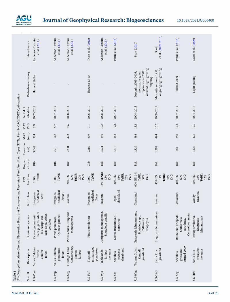
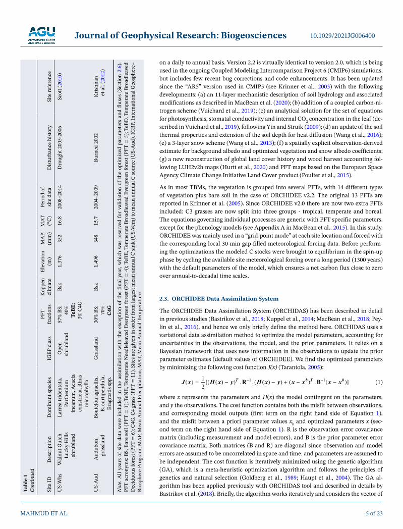
Twelve semi-arid eddy covariance flux sites in the southwestern US (SW US) have been utilized in this study, with a measurement period ranging between 2003 and 2014. These sites have a range of different vegetation types, climates, elevation and have been described in detail by Biederman et al. (2017), so we only provide a brief description here. We summarize the sites' description, dominant vegetation species, mean climate and corresponding vegetation plant functional types (PFTs), together with the observation period and disturbance history (Table 1). The sites are listed consecutively based on their mean annual C balance in Table 1. The major regional IGBP vegetation classes represented include evergreen needleleaf forest, woody savanna, open and closed shrubland, and grassland. These sites typically experience monsoon rainfall during July to October, preceded by a hot, dry period in May and June. The SW US is characterized by water limitation at the annual scale, that is, potential ET is greater than precipitation. The sites have large spatial gradients in mean annual precipitation (MAP 250–724 mm) and temperature (MAT 2.9–17.7°C) due to interactions among topography, latitude, wind patterns, and distance from oceans. For further site details, see references in Table 1 and individual site pages on www.ameriflux.lbl.gov.

2.2. ORCHIDEE Terrestrial Biosphere Model

We used the ORCHIDEE (ORganizing Carbon and Hydrology In Dynamic EcosystEms) process-oriented land surface model version 2.2 that has been developed at the IPSL (Institut Pierre Simon Laplace, France). The model is a state-of-the-art mechanistic terrestrial biosphere model (Krinner et  al.,  2005) and is the land surface component of the IPSLCM5 Earth System Model (Dufresne et al., 2013). The model describes the exchanges of water, carbon, and energy between biosphere and atmosphere at the smallest time scale (30 min), while the slow components of the terrestrial carbon cycle (including carbon allocation, autotroph-ic respiration, foliar onset and senescence, mortality and soil organic matter decomposition) are computed

Journal of Geophysical Research: Biogeosciences

MAHMUD ET AL.

10.1029/2021JG006400

4 of 23

Site

IDD

escr

iptio

nD

omin

ant s

peci

esIG

BP c

lass

PFT

frac

tions

Kop

pen

clim

ate

Elev

atio

n (m

)M

AP

(mm

)M

AT

(°C

)Pe

riod

of

site

dat

aD

istu

rban

ce h

isto

rySi

te re

fere

nce

US-

Vcm

Valle

s Cal

dera

m

ixed

co

nife

r fo

rest

Pice

a en

gelm

anni

i, Pi

cea

puge

ns, A

bies

la

sioc

arpa

var

. la

sioc

arpa

, Abi

es

conc

olor

Ever

gree

n ne

edle

leaf

Fo

rest

100%

Te

NE

Dfb

3,04

272

42.

920

07–2

012

Har

vest

196

0sA

nder

son-

Teix

eira

et

 al. 

(201

1)

US-

Vcp

Valle

s Cal

dera

po

nder

osa

fore

st

Pinu

s pon

dero

sa,

Que

rcus

gam

beli

Ever

gree

n ne

edle

leaf

Fo

rest

100%

Te

NE

Dfb

2501

547

5.7

2007

–201

4-

And

erso

n-Te

ixei

ra

et a

l. (2

011)

US-

Mpj

Her

itage

Lan

d C

onse

rvan

cy

piny

on-

juni

per

Pinu

s edu

lis, J

unip

erus

m

onos

perm

aSa

vann

a20

% B

S;

60%

Te

NE

; 20

%

C4G

Bsk

2200

423

9.6

2008

–201

4-

And

erso

n-Te

ixei

ra

et a

l. (2

011)

US-

Fuf

Flag

staf

f un

man

aged

po

nder

osa

Pinu

s pon

dero

saEv

ergr

een

need

lele

af

Fore

st

100%

Te

NE

Csb

2215

607

7.1

2006

–201

0H

arve

st 1

,910

Dor

e et

 al. 

(201

2)

US-

Wjs

Tabl

elan

ds

juni

per

sava

nna

Juni

peru

s mon

ospe

rma,

Bo

utel

oua

grac

ilis

Sava

nna

15%

TeN

E;

85%

C

4G

Bsk

1,93

134

910

.920

08–2

014

-A

nder

son-

Teix

eira

et

 al. 

(201

1)

US-

Ses

Sevi

lleta

cr

eoso

te

shru

blan

d

Larr

ea tr

iden

tata

, G.

saro

thra

eO

pen

shru

blan

d20

% B

S;

55%

Te

BE

; 25

%

C4G

Bsk

1,61

025

212

.620

07–2

014

-Pe

trie

et a

l. (2

015)

US-

Wkg

Wal

nut G

ulch

K

enda

ll gr

assl

and

Erag

rost

is le

hman

nian

a,

Bout

elou

a sp

p.

Cal

liand

ra

erio

phyl

la

Gra

ssla

nd60

% B

S; 3

%

TeBE

; 37

%

C4G

Bsk

1,52

938

615

.820

04–2

013

Dro

ught

200

3–20

05,

non-

nativ

e gr

ass

repl

acem

ent 2

007

onw

ard,

ligh

t gra

zing

on

goin

g

Scot

t (20

10)

US-

SRG

Sant

a R

ita

gras

slan

dEr

agro

stis

lehm

anni

ana

Sava

nna

45%

BS;

11

%

TeB

D;

44%

C

4G

Bsh

1,29

249

416

.720

09–2

014

Mes

quite

rem

oval

195

7,

ongo

ing

light

gra

zing

Scot

t et

 al. 

(200

9, 2

015)

US-

Seg

Sevi

lleta

gr

assl

and:

bu

rned

200

9

Bout

elou

a er

iopo

da,

Gut

ierr

ezia

sa

roth

rae,

C

erat

oide

s lan

ata

Gra

ssla

nd40

% B

S;

60%

C

4G

Bsk

160

250

12.6

2007

–201

4Bu

rned

 200

9Pe

trie

et a

l. (2

015)

US-

SRM

Sant

a R

ita

mes

quite

sa

vann

a

Pros

opis

vel

utin

a,

Erag

rost

is

lehm

anni

ana

Woo

dy

sava

nna

50%

BS;

35

%

TeB

D;

15%

C

4G

Bsk

1,12

242

117

.720

04–2

014

Ligh

t gra

zing

Scot

t et a

l. (2

009)

Tabl

e 1

Site

Des

crip

tions

, Mea

n Cl

imat

e, O

bser

vatio

n Ye

ars,

and

Corr

espo

ndin

g Veg

etat

ion

Plan

t Fun

ctio

nal T

ypes

(PFT

s) U

sed

in O

RCH

IDEE

Opt

imiz

atio

n

Journal of Geophysical Research: Biogeosciences

MAHMUD ET AL.

10.1029/2021JG006400

5 of 23

on a daily to annual basis. Version 2.2 is virtually identical to version 2.0, which is being used in the ongoing Coupled Modeling Intercomparison Project 6 (CMIP6) simulations, but includes few recent bug corrections and code enhancements. It has been updated since the “AR5” version used in CMIP5 (see Krinner et  al.,  2005) with the following developments: (a) an 11-layer mechanistic description of soil hydrology and associated modifications as described in MacBean et al. (2020); (b) addition of a coupled carbon-ni-trogen scheme (Vuichard et al., 2019); (c) an analytical solution for the set of equations for photosynthesis, stomatal conductivity and internal CO2 concentration in the leaf (de-scribed in Vuichard et al., 2019), following Yin and Struik (2009); (d) an update of the soil thermal properties and extension of the soil depth for heat diffusion (Wang et al., 2016); (e) a 3-layer snow scheme (Wang et al., 2013); (f) a spatially explicit observation-derived estimate for background albedo and optimized vegetation and snow albedo coefficients; (g) a new reconstruction of global land cover history and wood harvest accounting fol-lowing LUH2v2h maps (Hurtt et al., 2020) and PFT maps based on the European Space Agency Climate Change Initiative Land Cover product (Poulter et al., 2015).

As in most TBMs, the vegetation is grouped into several PFTs, with 14 different types of vegetation plus bare soil in the case of ORCHIDEE v2.2. The original 13 PFTs are reported in Krinner et al. (2005). Since ORCHIDEE v2.0 there are now two extra PFTs included: C3 grasses are now split into three groups - tropical, temperate and boreal. The equations governing individual processes are generic with PFT specific parameters, except for the phenology models (see Appendix A in MacBean et al., 2015). In this study, ORCHIDEE was mainly used in a “grid-point mode” at each site location and forced with the corresponding local 30-min gap-filled meteorological forcing data. Before perform-ing the optimizations the modeled C stocks were brought to equilibrium in the spin-up phase by cycling the available site meteorological forcing over a long period (1300 years) with the default parameters of the model, which ensures a net carbon flux close to zero over annual-to-decadal time scales.

2.3. ORCHIDEE Data Assimilation System

The ORCHIDEE Data Assimilation System (ORCHIDAS) has been described in detail in previous studies (Bastrikov et al., 2018; Kuppel et al., 2014; MacBean et al., 2018; Pey-lin et al., 2016), and hence we only briefly define the method here. ORCHIDAS uses a variational data assimilation method to optimize the model parameters, accounting for uncertainties in the observations, the model, and the prior parameters. It relies on a Bayesian framework that uses new information in the observations to update the prior parameter estimates (default values of ORCHIDEE). We find the optimized parameters by minimizing the following cost function J(x) (Tarantola, 2005):

J x H x y H x y x x x xT b T b( ) [( ( ) ) . . ( ) ) ( . ( ]( ) ) 1

2

1 1R B (1)

where x represents the parameters and H(x) the model contingent on the parameters, and y the observations. The cost function contains both the misfit between observations, and corresponding model outputs (first term on the right hand side of Equation  1), and the misfit between a priori parameter values xb and optimized parameters x (sec-ond term on the right hand side of Equation 1). R is the observation error covariance matrix (including measurement and model errors), and B is the prior parameter error covariance matrix. Both matrices (B and R) are diagonal since observation and model errors are assumed to be uncorrelated in space and time, and parameters are assumed to be independent. The cost function is iteratively minimized using the genetic algorithm (GA), which is a meta-heuristic optimization algorithm and follows the principles of genetics and natural selection (Goldberg et  al.,  1989; Haupt et  al.,  2004). The GA al-gorithm has been applied previously with ORCHIDAS tool and described in details by Bastrikov et al. (2018). Briefly, the algorithm works iteratively and considers the vector of Ta

ble

1 Co

ntin

ued

Site

IDD

escr

iptio

nD

omin

ant s

peci

esIG

BP c

lass

PFT

frac

tions

Kop

pen

clim

ate

Elev

atio

n (m

)M

AP

(mm

)M

AT

(°C

)Pe

riod

of

site

dat

aD

istu

rban

ce h

isto

rySi

te re

fere

nce

US-

Whs

Wal

nut G

ulch

Lu

cky

Hill

s sh

rubl

and

Larr

ea tr

iden

tata

, Pa

rthe

nium

in

canu

m, A

caci

a co

nstr

icta

, Rhu

s m

icro

phyl

la

Ope

n sh

rubl

and

57%

BS;

40

%

TeB

E;

3% C

4G

Bsk

1,37

635

216

.820

08–2

014

Dro

ught

200

5-20

06Sc

ott (

2010

)

US-

Aud

Aud

ubon

gr

assl

and

Bout

elou

agr

acili

s, B.

cur

tipen

dula

, Er

agro

stis

spp.

Gra

ssla

nd30

% B

S;

70%

C

4G

Bsk

1,49

634

815

.720

04–2

009

Burn

ed 2

002

Kri

shna

n et

 al. 

(201

2)

Not

e. A

ll ye

ars

of s

ite d

ata

wer

e in

clud

ed in

the

assi

mila

tion

with

the

exce

ptio

n of

the

final

yea

r, w

hich

was

res

erve

d fo

r va

lidat

ion

of th

e op

timiz

ed p

aram

eter

s an

d flu

xes

(Sec

tion 

2.6)

. PF

T ac

rony

ms:

BS, B

are

soil

(PFT

 = 1

); Te

NE,

Tem

pera

te N

eedl

elea

ved

Ever

gree

n fo

rest

(PFT

 = 4

); Te

BE, T

empe

rate

Bro

adle

aved

Eve

rgre

en fo

rest

(PFT

 = 5

); Te

BD, T

empe

rate

Bro

adle

aved

D

ecid

uous

fore

st (P

FT =

 6);

C4G

, C4

gras

s (PF

T =

 11)

. Site

s are

giv

en in

ord

er fr

om la

rges

t mea

n an

nual

C si

nk (U

S-Vc

m) t

o m

ean

annu

al C

sour

ce (U

S-A

ud).

IGBP

, Int

erna

tiona

l Geo

sphe

re–

Bios

pher

e Pr

ogra

m; M

AP,

Mea

n A

nnua

l Pre

cipi

tatio

n; M

AT,

Mea

n A

nnua

l Tem

pera

ture

.

Journal of Geophysical Research: Biogeosciences

MAHMUD ET AL.

10.1029/2021JG006400

6 of 23

parameters as a chromosome and each parameter as a gene on that chromosome. The method fills a set of n chromosomes at every iteration, having the starting pool as a randomly perturbed parameter pool. The chro-mosomes at each subsequent iteration are chosen from randomly selected chromosomes of the previous iteration by either “crossover” or “mutation” process. Santaren et al. (2014) showed that the performance of the algorithm is highly sensitive to its specific configuration and found the best configuration based on computational efficiency after testing different options. Here, we used the same configuration (i.e., number of chromosomes in the pool is the total number of parameters optimized; the number of iterations is 40; crossover/mutation ratio is 4:1; the number of gene blocks exchanged during crossover is 2 and the number of genes perturbed during mutation is 1) applied by Santaren et al. (2014) and Bastrikov et al. (2018). The algorithm does not assume prior knowledge of Gaussian probability distribution functions (PDFs) for the observation and parameter uncertainties; however, we do assume Gaussian errors for both R and B in this study. Given we do not fully know the model uncertainty, we set the prior observation uncertainty as the RMSE between the model and the observations following Kuppel et al. (2014). The prior parameter uncer-tainties are listed in Table S1.

The posterior error covariance matrix of the parameters (A) can be estimated by:

A R B [ ]H HT 1 1 1 (2)

This computes error correlations between parameters with the assumption of Gaussian prior errors and linearity of the model in the vicinity of the solution.

2.4. Flux Tower Measurements

At all 12 SW US sites, flux tower instruments collect 30-min measurements of meteorological forcing data and eddy covariance measurements of net surface energy and carbon exchanges, which are available from the AmeriFlux data portal (http://ameriflux.lbl.gov). Meteorological forcing data included air temperature and surface pressure, precipitation, incoming long and shortwave radiation, wind speed, and specific hu-midity. To run the ORCHIDEE model, we partitioned the in-situ precipitation into rain and snowfall using a temperature threshold of 0°C. The site-level meteorological forcing data were gap filled utilizing down-scaled and corrected ERA-Interim data following the approach of Vuichard and Papale (2015). Gross prima-ry productivity (GPP) and the ecosystem respiration (Reco) were estimated from the net ecosystem exchange (NEE) via the flux partitioning method described in Biederman et al. (2016). We acknowledge that GPP and Reco are not fully independent data with respect to NEE and are essentially model-derived estimates, but these concerns have been largely discussed in previous studies for example, Desai et al. (2008). Note that in this study, negative NEE refers to net CO2 uptake into the ecosystem. In order to exclude the influence of the short-term variations in the fluxes on the model optimization, the daily averaged observations smoothed with a 15-day running mean were used in the assimilation as per Bastrikov et al. (2018).

2.5. Parameters Optimized

The full set of parameters included in the assimilations optimized are described in Table S1 with their prior values, prior uncertainty, and upper and lower bounds for different PFTs based on literature analysis, pa-rameter databases and expert knowledge of the model equations. Prior values are the default parameter val-ues used in all non-optimized ORCHIDEE simulations. In the most past ORCHIDAS studies with previous versions of ORCHIDEE, only subsets of ORCHIDEE C cycle parameters have been optimized (Bastrikov et al., 2018; Kuppel et al., 2012, 2014; MacBean et al., 2015, 2018; Santaren et al., 2007; Verbeeck et al., 2011). In this study, we considered all possible C cycle related ORCHIDEE parameters to fully explore all sources of parameter uncertainty that is contributing to uncertainties in modeled net and gross CO2 fluxes. We fur-ther allowed weak constraints in the DA system (i.e., large prior parameter bounds, albeit within realistic limits) because the main objective of our study was to determine if parameter calibration can improve the model-data fit within the existing model structure and to use our assimilation scenario tests to identify which processes are responsible for model-data errors.

We identified three main groups of parameters: parameters related to (a) phenology; (b) photosynthesis; and (c) all process calculations that occur after gross C uptake (i.e., C allocation, autotrophic and heterotrophic

Journal of Geophysical Research: Biogeosciences

MAHMUD ET AL.

10.1029/2021JG006400

7 of 23

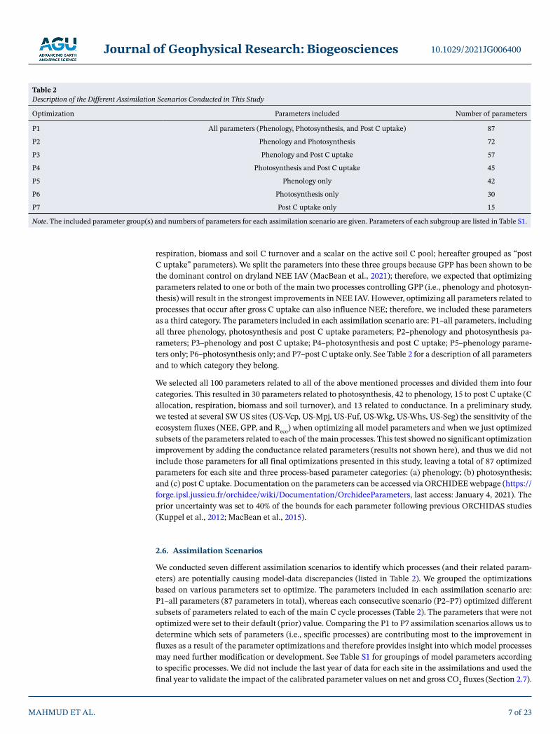
respiration, biomass and soil C turnover and a scalar on the active soil C pool; hereafter grouped as “post C uptake” parameters). We split the parameters into these three groups because GPP has been shown to be the dominant control on dryland NEE IAV (MacBean et al., 2021); therefore, we expected that optimizing parameters related to one or both of the main two processes controlling GPP (i.e., phenology and photosyn-thesis) will result in the strongest improvements in NEE IAV. However, optimizing all parameters related to processes that occur after gross C uptake can also influence NEE; therefore, we included these parameters as a third category. The parameters included in each assimilation scenario are: P1–all parameters, including all three phenology, photosynthesis and post C uptake parameters; P2–phenology and photosynthesis pa-rameters; P3–phenology and post C uptake; P4–photosynthesis and post C uptake; P5–phenology parame-ters only; P6–photosynthesis only; and P7–post C uptake only. See Table 2 for a description of all parameters and to which category they belong.

We selected all 100 parameters related to all of the above mentioned processes and divided them into four categories. This resulted in 30 parameters related to photosynthesis, 42 to phenology, 15 to post C uptake (C allocation, respiration, biomass and soil turnover), and 13 related to conductance. In a preliminary study, we tested at several SW US sites (US-Vcp, US-Mpj, US-Fuf, US-Wkg, US-Whs, US-Seg) the sensitivity of the ecosystem fluxes (NEE, GPP, and Reco) when optimizing all model parameters and when we just optimized subsets of the parameters related to each of the main processes. This test showed no significant optimization improvement by adding the conductance related parameters (results not shown here), and thus we did not include those parameters for all final optimizations presented in this study, leaving a total of 87 optimized parameters for each site and three process-based parameter categories: (a) phenology; (b) photosynthesis; and (c) post C uptake. Documentation on the parameters can be accessed via ORCHIDEE webpage (https://forge.ipsl.jussieu.fr/orchidee/wiki/Documentation/OrchideeParameters, last access: January 4, 2021). The prior uncertainty was set to 40% of the bounds for each parameter following previous ORCHIDAS studies (Kuppel et al., 2012; MacBean et al., 2015).

2.6. Assimilation Scenarios

We conducted seven different assimilation scenarios to identify which processes (and their related param-eters) are potentially causing model-data discrepancies (listed in Table 2). We grouped the optimizations based on various parameters set to optimize. The parameters included in each assimilation scenario are: P1–all parameters (87 parameters in total), whereas each consecutive scenario (P2–P7) optimized different subsets of parameters related to each of the main C cycle processes (Table 2). The parameters that were not optimized were set to their default (prior) value. Comparing the P1 to P7 assimilation scenarios allows us to determine which sets of parameters (i.e., specific processes) are contributing most to the improvement in fluxes as a result of the parameter optimizations and therefore provides insight into which model processes may need further modification or development. See Table S1 for groupings of model parameters according to specific processes. We did not include the last year of data for each site in the assimilations and used the final year to validate the impact of the calibrated parameter values on net and gross CO2 fluxes (Section 2.7).

Optimization Parameters included Number of parameters

P1 All parameters (Phenology, Photosynthesis, and Post C uptake) 87

P2 Phenology and Photosynthesis 72

P3 Phenology and Post C uptake 57

P4 Photosynthesis and Post C uptake 45

P5 Phenology only 42

P6 Photosynthesis only 30

P7 Post C uptake only 15

Note. The included parameter group(s) and numbers of parameters for each assimilation scenario are given. Parameters of each subgroup are listed in Table S1.

Table 2 Description of the Different Assimilation Scenarios Conducted in This Study

Journal of Geophysical Research: Biogeosciences

MAHMUD ET AL.

10.1029/2021JG006400

8 of 23

2.7. Post-Optimization Analysis

For all assimilation scenarios we compared the prior simulation (before parameter optimization) to the posterior simulations (after parameter optimization, with different parameter groupings for the different assimilation scenarios) by evaluating the simulations against the site data using standard goodness of fit metrics (root mean square error, RMSE and Pearson correlation coefficient, R) at daily, monthly and in-ter-annual timescales. We further attributed what might be causing model-data misfits by decomposing the daily mean squared deviation (MSD) into its component phase, variance and bias contributions following the approach of Kobayashi and Salam (2000). The bias, variance and phase indicate the mean difference in flux magnitude, the mismatch in terms of the magnitude of fluctuations, and the seasonality in flux time series, respectively (Kobayashi & Salam, 2000). We calculated the MSD between daily model and observed time series and decompose it following the equation:

MSD

12 1

1

2 2 2

nx y x y R

i

n

i i x y x y( ) ( ) ( ) ( ) (3)

where x is the model and y is the observations, σ is the standard deviation and R is the correlation coeffi-cient. The first term specifies the bias between model simulation and observation (squared). The second “variance” term measures their differences in terms of variability (i.e., the difference between the magni-tude of the modeled and observed fluctuations). The third term in Equation 3 generally demonstrates the lack of correlation between model and observations weighted by their standard deviations, which can be deemed a measure of their disagreement in terms in phase (Bacour et al., 2019; Gauch et al., 2003). We further calculated the contribution of each component (bias, variance and phase) to the overall MSD by dividing each component by the total MSD. Model evaluation metrics are presented in one of three ways: (a) for each site; (b) grouped across all sites; and (c) sites grouped according to their mean net annual CO2 flux characteristics across the observed time period as in Biederman et al. (2017). For the latter, the net CO2 “sink” sites are US-Vcm, US-Vcp, US-Mpj, US-Fuf, US-Wjs and US-Ses; the “pivot” sites are US-Wkg, US-SRG, US-SRM, US-Whs, US-Seg; and the “source” site is US-Aud.

We performed a temporal validation at each site and for each assimilation scenario by comparing the mod-eled and observed daily NEE, GPP, and Reco RMSE and R during the validation window (using the final year of data that was excluded from the assimilation). The impact of the temporal validation tests is presented in Section 3.1 and 3.2. All other model evaluation metrics refer to the assimilation time window. We also evaluated the posterior parameter values using the limited available trait data close to the sites from the TRY database (Kattge et al., 2020). We searched within 0.5° of the latitude and longitude of each site for trait data related to the species present at each site. We found one estimate of specific leaf area (SLA) for pinus ponderosa close to US-Fuf, and maximum rate of rubisco activity-limited carboxylation at 25°C (Vc,max) and leaf longevity estimates for larrea tridentata (creosote shrubs) close to US-Ses. The comparison of these trait values to posterior parameter estimates is presented in Section 3.3.

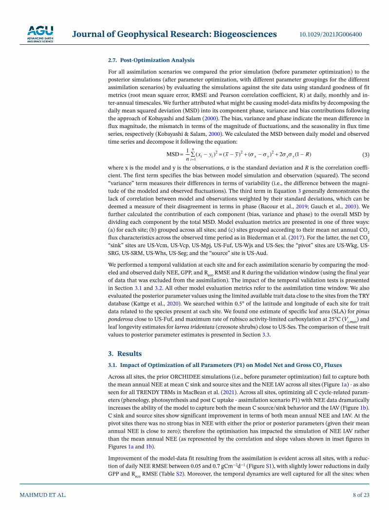
3. Results3.1. Impact of Optimization of all Parameters (P1) on Model Net and Gross CO2 Fluxes

Across all sites, the prior ORCHIDEE simulations (i.e., before parameter optimization) fail to capture both the mean annual NEE at mean C sink and source sites and the NEE IAV across all sites (Figure 1a) - as also seen for all TRENDY TBMs in MacBean et al. (2021). Across all sites, optimizing all C cycle-related param-eters (phenology, photosynthesis and post C uptake - assimilation scenario P1) with NEE data dramatically increases the ability of the model to capture both the mean C source/sink behavior and the IAV (Figure 1b). C sink and source sites show significant improvement in terms of both mean annual NEE and IAV. At the pivot sites there was no strong bias in NEE with either the prior or posterior parameters (given their mean annual NEE is close to zero); therefore the optimisation has impacted the simulation of NEE IAV rather than the mean annual NEE (as represented by the correlation and slope values shown in inset figures in Figures 1a and 1b).

Improvement of the model-data fit resulting from the assimilation is evident across all sites, with a reduc-tion of daily NEE RMSE between 0.05 and 0.7 gCm−2d−1 (Figure S1), with slightly lower reductions in daily GPP and Reco RMSE (Table S2). Moreover, the temporal dynamics are well captured for all the sites: when

Journal of Geophysical Research: Biogeosciences

MAHMUD ET AL.

10.1029/2021JG006400

9 of 23

optimizing all parameters, the median R increase by 0.45, 0.45, and 0.3 for daily, monthly and annual mod-eled NEE, respectively and posterior median slope increase by ≥ 0.35 at all timescales (Figure S2a and S2d). GPP temporal dynamics are also much improved by the P1 assimilation with a higher median value and tighter range in posterior R and slope values at all timescales (Figure S2b and S2e). In contrast, there is less improvement in Reco temporal dynamics although the median R and slope values are higher after the opti-mization with the exception of the annual values (Figure S2c and S2f).

The median daily NEE RMSE and R for the temporal validation analysis indicates that the optimized pa-rameters maintain an improved model-data fit outside the assimilation window when compared to the prior (Figure S3). The median value of daily NEE RMSE is 0.1 higher for the validation test compared to the assimilation for the P1 assimilation scenario; however, the maximum to minimum range of RMSE values in the validation is very similar to original optimization and much less than the prior simulation (Figure S3a). Similarly, the median R of daily NEE is slightly less for the validation test than the original optimization for P1 (Figure S3b). The daily GPP RMSE and R show similar model-data fit for the validation analysis of the P1 optimized parameters as the original optimizations (results not shown). However, the median daily Reco is the same for the prior, optimization and validation, while there is an increasing improvements in the median daily Reco R for both the P1 optimization and validation (results not shown).

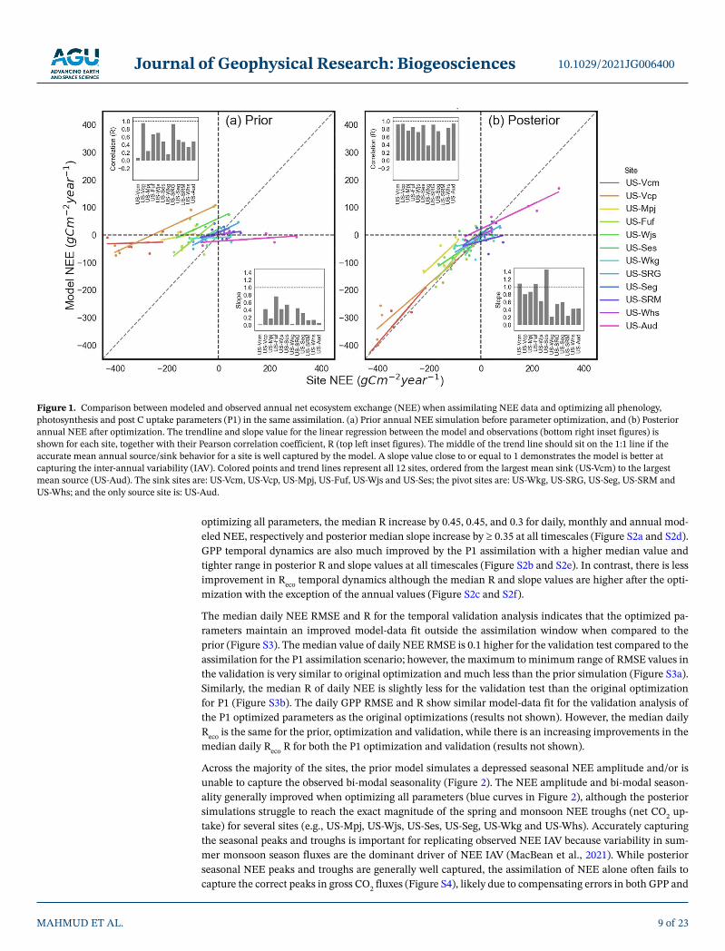
Across the majority of the sites, the prior model simulates a depressed seasonal NEE amplitude and/or is unable to capture the observed bi-modal seasonality (Figure 2). The NEE amplitude and bi-modal season-ality generally improved when optimizing all parameters (blue curves in Figure 2), although the posterior simulations struggle to reach the exact magnitude of the spring and monsoon NEE troughs (net CO2 up-take) for several sites (e.g., US-Mpj, US-Wjs, US-Ses, US-Seg, US-Wkg and US-Whs). Accurately capturing the seasonal peaks and troughs is important for replicating observed NEE IAV because variability in sum-mer monsoon season fluxes are the dominant driver of NEE IAV (MacBean et al., 2021). While posterior seasonal NEE peaks and troughs are generally well captured, the assimilation of NEE alone often fails to capture the correct peaks in gross CO2 fluxes (Figure S4), likely due to compensating errors in both GPP and

Figure 1. Comparison between modeled and observed annual net ecosystem exchange (NEE) when assimilating NEE data and optimizing all phenology, photosynthesis and post C uptake parameters (P1) in the same assimilation. (a) Prior annual NEE simulation before parameter optimization, and (b) Posterior annual NEE after optimization. The trendline and slope value for the linear regression between the model and observations (bottom right inset figures) is shown for each site, together with their Pearson correlation coefficient, R (top left inset figures). The middle of the trend line should sit on the 1:1 line if the accurate mean annual source/sink behavior for a site is well captured by the model. A slope value close to or equal to 1 demonstrates the model is better at capturing the inter-annual variability (IAV). Colored points and trend lines represent all 12 sites, ordered from the largest mean sink (US-Vcm) to the largest mean source (US-Aud). The sink sites are: US-Vcm, US-Vcp, US-Mpj, US-Fuf, US-Wjs and US-Ses; the pivot sites are: US-Wkg, US-SRG, US-Seg, US-SRM and US-Whs; and the only source site is: US-Aud.

Journal of Geophysical Research: Biogeosciences

MAHMUD ET AL.

10.1029/2021JG006400

10 of 23

Reco. We note however that the mean seasonal cycle for the gross CO2 fluxes is generally much improved, especially for low-elevation “pivot” sites with a clear bi-modal growing season (e.g., US-Wkg, US-SRM, US-SRG, and US-Whs: Figure S4). At the C source site (US-Aud) the model also fails to simulate the accurate peak in mean springtime net carbon release (Figure 2). This is due to the fact that at US-Aud, TBMs tend to overestimate spring GPP and underestimate the earlier rise in spring Reco (Figure S4). The optimization only partially corrects these model biases, suggesting that other missing processes may ultimately be responsible for the model-data misfit (such as disturbance following a fire that occurred at the site in 2002, which is not implemented in the current version of ORCHIDEE).

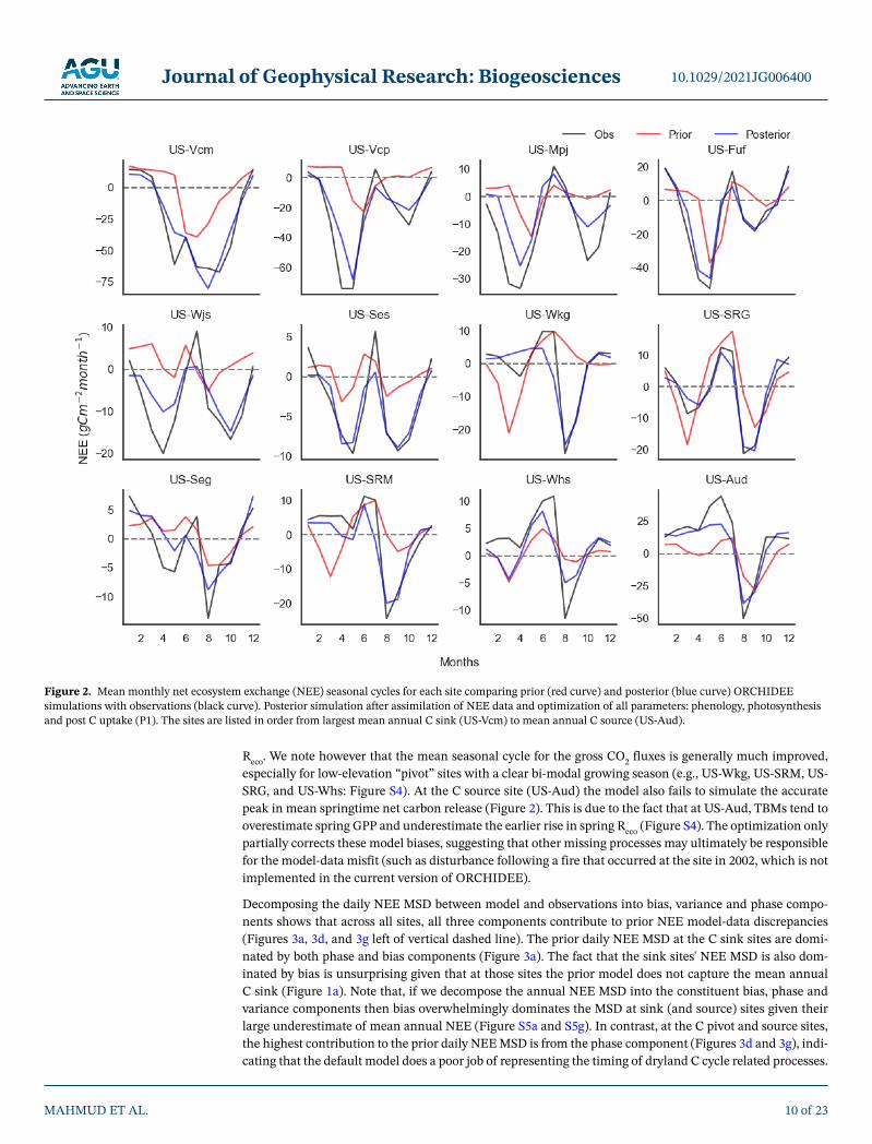
Decomposing the daily NEE MSD between model and observations into bias, variance and phase compo-nents shows that across all sites, all three components contribute to prior NEE model-data discrepancies (Figures 3a, 3d, and 3g left of vertical dashed line). The prior daily NEE MSD at the C sink sites are domi-nated by both phase and bias components (Figure 3a). The fact that the sink sites' NEE MSD is also dom-inated by bias is unsurprising given that at those sites the prior model does not capture the mean annual C sink (Figure 1a). Note that, if we decompose the annual NEE MSD into the constituent bias, phase and variance components then bias overwhelmingly dominates the MSD at sink (and source) sites given their large underestimate of mean annual NEE (Figure S5a and S5g). In contrast, at the C pivot and source sites, the highest contribution to the prior daily NEE MSD is from the phase component (Figures 3d and 3g), indi-cating that the default model does a poor job of representing the timing of dryland C cycle related processes.

Figure 2. Mean monthly net ecosystem exchange (NEE) seasonal cycles for each site comparing prior (red curve) and posterior (blue curve) ORCHIDEE simulations with observations (black curve). Posterior simulation after assimilation of NEE data and optimization of all parameters: phenology, photosynthesis and post C uptake (P1). The sites are listed in order from largest mean annual C sink (US-Vcm) to mean annual C source (US-Aud).

Journal of Geophysical Research: Biogeosciences

MAHMUD ET AL.

10.1029/2021JG006400

11 of 23

Across all sites, optimizing all parameters (P1) dramatically reduces the bias, variance and phase compo-nents of the daily NEE MSD, with phase remaining the strongest contributor to daily NEE MSD (Figures 3a, 3d, and 3g right of dashed line).

The bias and phase are the dominant contributors to prior daily GPP MSD for the sink sites (left of vertical dashed line in Figure 3b), and phase only for the pivot and source sites (Figures 3e and 3h). For Reco, a differ-ent MSD component is dominant depending on the mean C behavior of a site: bias dominates the prior daily Reco MSD at the sink sites, variance at the pivot sites, and phase at the source sites (Figures 3c, 3f, and 3i). Overall, assimilating NEE data in the P1 assimilation scenario reduces all gross CO2 flux MSD components (right of dashed line in Figure 3 middle and right columns), with phase remaining the strongest contributor to daily gross CO2 flux MSD at sink and source sites. However, unlike for the NEE, at the C sink sites phase and bias remain strong contributors to posterior GPP MSD (Figure 3b).

3.2. Impact of Different Processes (Assimilation Scenarios) on Optimization Results

Across all sites, modeled annual and seasonal NEE are improved the most in the P1 assimilation scenario, although all scenarios result in some improvement (Figures S6, S7a, and S7d, and seasonal cycles in Fig-ure S8). In general, there is less improvement in Reco compared to NEE and GPP (Figure S7). Examining the daily NEE median RMSE for the temporal validation analysis for the P2 to P7 assimilation scenarios shows that the optimized parameters have improved the model-data fit outside the assimilation window when compared to the prior, with the exception of scenarios that include photosynthesis or post C uptake

Figure 3. Daily net ecosystem exchange (NEE), gross primary productivity (GPP) and ecosystem respiration (Reco) mean square deviation (MSD) decomposition into bias, variance, and phase between simulations and observations for assimilating NEE observations and optimizing all phenology, photosynthesis and post C uptake parameters (P1). Blue, orange and green boxplots represent bias, variance and phase components, respectively. Different rows separate the sites as sink (a–c), pivot (d–f) and source (g–i) based on total annual C flux. The sink sites are: US-Vcm, US-Vcp, US-Mpj, US-Fuf, US-Wjs and US-Ses; the pivot sites are: US-Wkg, US-SRG, US-Seg, US-SRM and US-Whs; and the source site is: US-Aud. The x axes display the optimization scenarios (Prior and P1). The box whiskers show the spread of bias, variance and phase for all 12 sites considered in this study. The bias, variance and phase indicate the mean difference in flux magnitude, the mismatch in terms of flux fluctuation magnitude scales with the mean seasonal amplitude, and the seasonality in flux time series, respectively (see Methods). Note that the y axis limits for both gross fluxes (GPP and Reco) are the same.

Journal of Geophysical Research: Biogeosciences

MAHMUD ET AL.

10.1029/2021JG006400

12 of 23

parameters (e.g., P2, P4, P6, and P7 - Figure S3a). However, the range of RMSE values from the validation tests is similar to the original optimization and much less than the prior simulation for all optimization scenarios. Similarly, the median R between modeled and observed daily NEE for the validation test is higher than the prior for all assimilation scenarios and is close to the optimized median R (within ±0.1) for P2, P3, P5, and P7 (Figure S3b). The 25th percentile of the range in R values is generally higher than the prior for P2, P3, and P5, but not for P4, P6, and P7 (Figure S3b), which, again, are scenarios that include photosyn-thesis or post C uptake parameters but not parameters related to phenology.

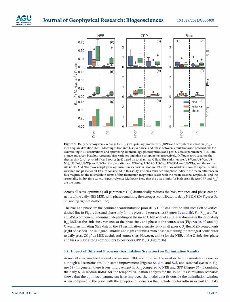
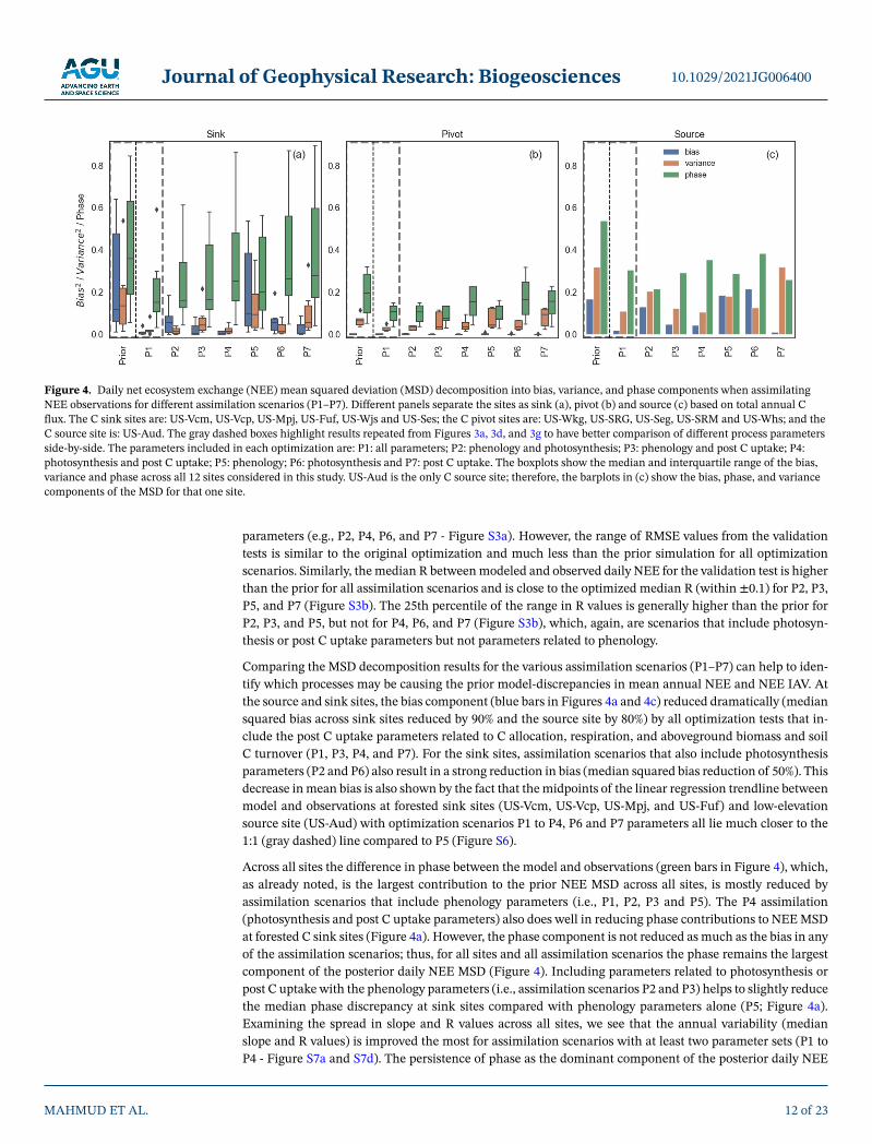
Comparing the MSD decomposition results for the various assimilation scenarios (P1–P7) can help to iden-tify which processes may be causing the prior model-discrepancies in mean annual NEE and NEE IAV. At the source and sink sites, the bias component (blue bars in Figures 4a and 4c) reduced dramatically (median squared bias across sink sites reduced by 90% and the source site by 80%) by all optimization tests that in-clude the post C uptake parameters related to C allocation, respiration, and aboveground biomass and soil C turnover (P1, P3, P4, and P7). For the sink sites, assimilation scenarios that also include photosynthesis parameters (P2 and P6) also result in a strong reduction in bias (median squared bias reduction of 50%). This decrease in mean bias is also shown by the fact that the midpoints of the linear regression trendline between model and observations at forested sink sites (US-Vcm, US-Vcp, US-Mpj, and US-Fuf) and low-elevation source site (US-Aud) with optimization scenarios P1 to P4, P6 and P7 parameters all lie much closer to the 1:1 (gray dashed) line compared to P5 (Figure S6).

Across all sites the difference in phase between the model and observations (green bars in Figure 4), which, as already noted, is the largest contribution to the prior NEE MSD across all sites, is mostly reduced by assimilation scenarios that include phenology parameters (i.e., P1, P2, P3 and P5). The P4 assimilation (photosynthesis and post C uptake parameters) also does well in reducing phase contributions to NEE MSD at forested C sink sites (Figure 4a). However, the phase component is not reduced as much as the bias in any of the assimilation scenarios; thus, for all sites and all assimilation scenarios the phase remains the largest component of the posterior daily NEE MSD (Figure 4). Including parameters related to photosynthesis or post C uptake with the phenology parameters (i.e., assimilation scenarios P2 and P3) helps to slightly reduce the median phase discrepancy at sink sites compared with phenology parameters alone (P5; Figure 4a). Examining the spread in slope and R values across all sites, we see that the annual variability (median slope and R values) is improved the most for assimilation scenarios with at least two parameter sets (P1 to P4 - Figure S7a and S7d). The persistence of phase as the dominant component of the posterior daily NEE

Figure 4. Daily net ecosystem exchange (NEE) mean squared deviation (MSD) decomposition into bias, variance, and phase components when assimilating NEE observations for different assimilation scenarios (P1–P7). Different panels separate the sites as sink (a), pivot (b) and source (c) based on total annual C flux. The C sink sites are: US-Vcm, US-Vcp, US-Mpj, US-Fuf, US-Wjs and US-Ses; the C pivot sites are: US-Wkg, US-SRG, US-Seg, US-SRM and US-Whs; and the C source site is: US-Aud. The gray dashed boxes highlight results repeated from Figures 3a, 3d, and 3g to have better comparison of different process parameters side-by-side. The parameters included in each optimization are: P1: all parameters; P2: phenology and photosynthesis; P3: phenology and post C uptake; P4: photosynthesis and post C uptake; P5: phenology; P6: photosynthesis and P7: post C uptake. The boxplots show the median and interquartile range of the bias, variance and phase across all 12 sites considered in this study. US-Aud is the only C source site; therefore, the barplots in (c) show the bias, phase, and variance components of the MSD for that one site.

Journal of Geophysical Research: Biogeosciences

MAHMUD ET AL.

10.1029/2021JG006400

13 of 23

suggests further model improvement in processes related to dryland vegetation temporal dynamics (e.g., phenology and all associated processes) is needed before TBMs can correctly reproduce NEE seasonality and IAV.

The variance component of the daily NEE MSD (orange bars in Figure 4), which shows a modest contri-bution to daily NEE MSD at the sink and source sites, is mostly reduced at the sink sites with assimilation scenarios that include photosynthesis parameters (i.e., P1, P2, P4 and P6 - Figure 4a). At US-Aud, which had a larger prior variance component than bias, the posterior variance was reduced by assimilation scenarios that tended to include photosynthesis or post C uptake parameters (i.e., P1, P3, P4 and P6; Figure 4c).

While the post C uptake parameters are key for reducing bias in forested sink site NEE, biases in GPP and Reco at these sites are reduced by optimizing photosynthesis parameters (P1, P2, P4, and P6 - blue boxes Figure S9b and S9c). The GPP and Reco bias components at the sink sites are not reduced as strongly as NEE biases for any assimilation scenario; thus, bias remains a key contributor to posterior gross CO2 flux MSD. Similarly to NEE, parameter subsets that include phenology parameters (P1, P2, P3 and P5) are key for reducing the daily GPP MSD sink and phase component at pivot sites (green boxes in Figure S9e; also see median GPP slope and R values in Figures S7b and S7e). With the exception of P1 and P2 for GPP, the GPP and Reco variance components are not reduced much by any of the assimilation scenarios and remain a considerable component of the MSD for both GPP and Reco at the pivot sites, and for Reco at the sink sites (Figures S9b, S9c, S9e, and S9f).

3.3. Constraint on Parameters

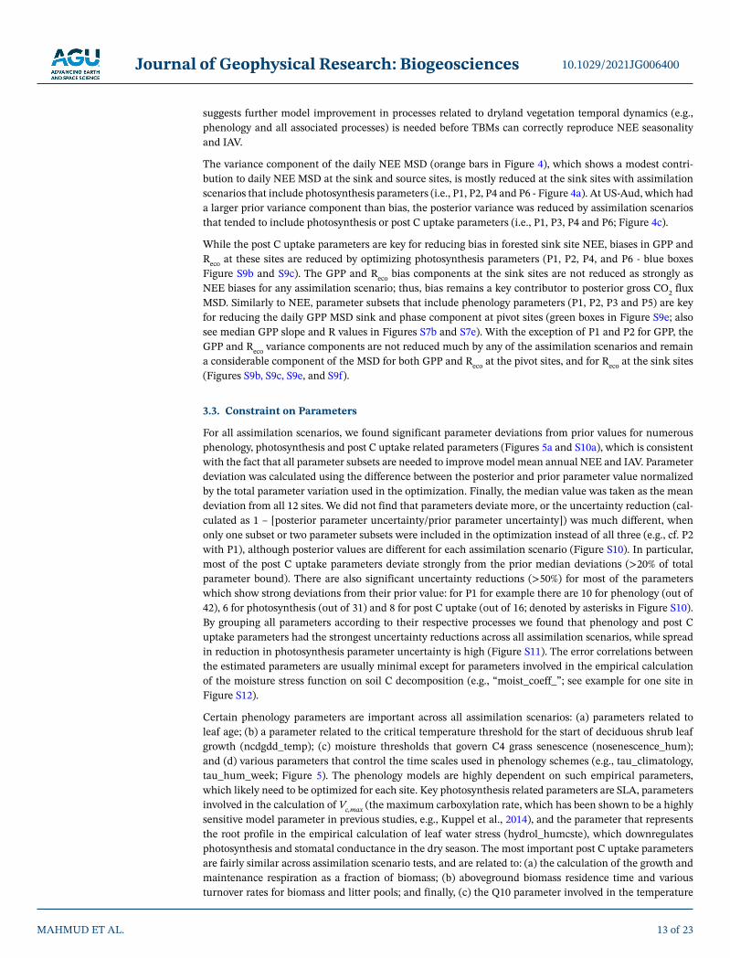
For all assimilation scenarios, we found significant parameter deviations from prior values for numerous phenology, photosynthesis and post C uptake related parameters (Figures 5a and S10a), which is consistent with the fact that all parameter subsets are needed to improve model mean annual NEE and IAV. Parameter deviation was calculated using the difference between the posterior and prior parameter value normalized by the total parameter variation used in the optimization. Finally, the median value was taken as the mean deviation from all 12 sites. We did not find that parameters deviate more, or the uncertainty reduction (cal-culated as 1 – [posterior parameter uncertainty/prior parameter uncertainty]) was much different, when only one subset or two parameter subsets were included in the optimization instead of all three (e.g., cf. P2 with P1), although posterior values are different for each assimilation scenario (Figure S10). In particular, most of the post C uptake parameters deviate strongly from the prior median deviations (>20% of total parameter bound). There are also significant uncertainty reductions (>50%) for most of the parameters which show strong deviations from their prior value: for P1 for example there are 10 for phenology (out of 42), 6 for photosynthesis (out of 31) and 8 for post C uptake (out of 16; denoted by asterisks in Figure S10). By grouping all parameters according to their respective processes we found that phenology and post C uptake parameters had the strongest uncertainty reductions across all assimilation scenarios, while spread in reduction in photosynthesis parameter uncertainty is high (Figure S11). The error correlations between the estimated parameters are usually minimal except for parameters involved in the empirical calculation of the moisture stress function on soil C decomposition (e.g., “moist_coeff_”; see example for one site in Figure S12).

Certain phenology parameters are important across all assimilation scenarios: (a) parameters related to leaf age; (b) a parameter related to the critical temperature threshold for the start of deciduous shrub leaf growth (ncdgdd_temp); (c) moisture thresholds that govern C4 grass senescence (nosenescence_hum); and (d) various parameters that control the time scales used in phenology schemes (e.g., tau_climatology, tau_hum_week; Figure  5). The phenology models are highly dependent on such empirical parameters, which likely need to be optimized for each site. Key photosynthesis related parameters are SLA, parameters involved in the calculation of Vc,max (the maximum carboxylation rate, which has been shown to be a highly sensitive model parameter in previous studies, e.g., Kuppel et al., 2014), and the parameter that represents the root profile in the empirical calculation of leaf water stress (hydrol_humcste), which downregulates photosynthesis and stomatal conductance in the dry season. The most important post C uptake parameters are fairly similar across assimilation scenario tests, and are related to: (a) the calculation of the growth and maintenance respiration as a fraction of biomass; (b) aboveground biomass residence time and various turnover rates for biomass and litter pools; and finally, (c) the Q10 parameter involved in the temperature

Journal of Geophysical Research: Biogeosciences

MAHMUD ET AL.

10.1029/2021JG006400

14 of 23

dependence of soil C decomposition (Figure 5). We compared the posterior parameter values for all relevant assimilation scenarios to the available trait data from the TRY database (Figure S13). The two photosynthe-sis traits (SLA for pinus ponderosa close to US-Fuf and Vc,max for larrea tridentata close to US-Ses were over- and underestimated by the posterior values across all assimilation scenarios, respectively, whereas the leaf longevity for larrea tridentata measured close to US-Ses was well captured by the P3 assimilation scenario. There is not enough trait information to perform a rigorous validation of the posterior parameter values. The existing measurements may differ from the model due to the fact that the traits were not measured at the same location. However, mismatches between the posterior parameter values and traits presented here highlights that we need to collect more trait data with which to evaluate the optimized parameters, in addition to using the DA framework to explore how parameters may vary over space and time. We discuss this further in Section 4.

Figure 5. Optimized median parameter deviations ([posterior - prior]/[max - min]; blue bars) and associated median parameter uncertainty reductions (gray bars) for parameters (having magnitude of deviation >0.3 or uncertainty reduction >50%) controlling phenology, photosynthesis and post C uptake assimilating net ecosystem exchange (NEE) data (P1–P7). Bars represent the median across all 12 sites. Each line corresponds to a specific optimization test (shown on the right axis). The parameters are given on the bottom axis. The vertical dashed lines separate the different parameter subsets (phenology, photosynthesis and post C uptake). Table S1 details the prior and posterior parameter values and their uncertainty for all parameters together with the maximum and minimum bounds used in the optimizations.

Journal of Geophysical Research: Biogeosciences

MAHMUD ET AL.

10.1029/2021JG006400

15 of 23

4. Discussion and Conclusions4.1. Further Testing and Developments Needed to Improve Modeling of Dryland C Cycling

In this study, we have shown that it is possible to account for model discrepancies in both the mean annual NEE and NEE IAV at a range of semi-arid SW US sites via optimization of C cycle parameters within a Bayesian DA framework. We used weak prior constraints (i.e., large prior parameter bounds) to give the as-similation the maximum chance to correct any model errors. Our goal was not to identify the ideal “correct” set of C cycle parameters for capturing semi-arid vegetation and C cycle dynamics, but rather to identify whether, within the current model representation, we could account for model-data mismatches. Looking at the individual parameter plots for the P1 assimilation scenario (Figure S14), we find that at some sites several posterior parameters are “edge-hitting” (e.g., soil Q10). Given we chose weak prior constraints in the assimilation, the fact that some posterior parameters are hitting their bounds suggests that the optimization may be aliasing model structural error onto the parameters (as demonstrated in MacBean et al., 2016; Wut-zler & Carvalhais, 2014) and/or that the model cannot improve further via parameter optimization. This suggests that further model developments are likely needed to address structural uncertainties and missing processes, which will then need to be followed up with additional parameter DA experiments to ensure increasing complexity does not degrade model skill (Famiglietti et al., 2021). We know for example that certain important processes for sparsely vegetated, mixed shrub- and grass-dominated dryland ecosystems, such as wildfires (Exbrayat et al., 2018; Lasslop et al., 2016; Whitley et al., 2017) and biological soil crust C cycling (Belnap et al., 2016), are currently not represented in most TBMs. Exbrayat et al. (2018) showed using a Bayesian parameter DA experiment that model simulations with fire had faster carbon turnover times and increased C allocation to wood and root pools (rather than foliage) than the simulations without fire–all of which resulted in changes to GPP, net primary productivity, biomass and carbon use efficiency. Their results neatly demonstrate that errors due to missing model processes can be aliased onto the poste-rior parameter values.

Hypotheses as to which processes might be responsible for model inability to capture semi-arid CO2 flux IAV–and therefore which processes need further development in the model–are numerous and will take time to explore fully. MacBean et al. (2021) suggested that the following processes might be causing model errors in capturing semi-arid C cycle dynamics: the lack of drought-deciduous shrub phenology schemes in TBMs (Renwick et al., 2019); the lack of deep tap roots for trees and shrubs that draw up groundwater needed for growth during drier periods (Gibbens & Lenz, 2001; Kerhoulas, et al., 2012); the lack of dynamic root growth or hydraulic redistribution as soil moisture changes with depth (De Kauwe et al., 2015; Fu et al., 2016; Lee et al., 2018; Li et al., 2012; Whitley et al., 2016, 2017); and inaccurate nutrient limitation in dryland ecosystems (Sun et al., 2021; Hooper & Johnson, 1999). Future studies need to systematically test all these options to determine which, if any, can explain the observed model-data discrepancies. Here, we aimed to facilitate our understanding of which processes may be responsible for errors in modeling of semi-arid C fluxes by using the different assimilation scenarios as tests of which parameter sets (and there-fore, which processes) most improve the model-data mismatch. The assimilation with all C cycle and vege-tation parameters (P1) performed the best in terms of correcting underestimates in modeled mean annual NEE and IAV. However, the additional assimilation scenarios (P2 to P7) further demonstrated that phenol-ogy parameters are likely key for improving semi-arid ecosystem NEE IAV. Issues with semi-arid phenology in TBMs have been documented elsewhere (Dahlin et al., 2015; MacBean et al., 2015; Renwick et al., 2019; Teckentrup et al., 2021 in review; Traore et al., 2014; Whitley et al., 2016). In addition, Wu et al. (2018) found that TBMs underestimate vegetation productivity responses to increased precipitation at grassland sites. Further evidence for inadequate TBM phenology schemes comes from MacBean et al. (2020), who noted that while the ORCHIDEE model can capture evapotranspiration (ET) fluxes extremely well, even without parameter optimization, the model simulates a delayed increase in transpiration/ET (T/ET) ratios during the summer monsoon when compared to two independent T/ET estimates. This suggests that the model is getting ET right for the wrong reasons–that is, the partitioning of ET into its component fluxes of T and bare soil evaporation is incorrect. This lagged response of T to increasing rainfall is consistent with the results of MacBean et al. (2021) who found across a suite of TBMs (TRENDY v7) too weak ecosystem-scale water use efficiency (WUE)–that is, a too weak response of GPP to increasing ET–during the monsoon was likely the cause of their inability to capture NEE IAV. Put simply, the models simulate too weak a response of

Journal of Geophysical Research: Biogeosciences

MAHMUD ET AL.

10.1029/2021JG006400

16 of 23

vegetation growth to pulses of moisture availability. Thus, the evidence from all these studies, including our results presented here, is pointing to issues with processes controlling seasonal vegetation dynamics such as phenology and plant hydraulics schemes that controls plant water stress.

Another source of error in the model NEE IAV simulations could be related to the fractional cover (fCover) of different PFTs prescribed in the model. Although we used site-based estimates of PFT fCover, these esti-mates typically represent the spatio-temporal average fCover at each site (as is often the case in coarse-scale (>30 m) satellite fCover estimates–Brandt et al., 2016). In contrast, the PFT fCover prescribed in TBMs should be the maximum possible fCover: The models then limit the growth of vegetation based on climate conditions and other resource availability. In the lower elevation sites, the in situ fCover estimates suggest a high fraction of bare soil at each site; however, in years with strong monsoon rainfall, growth of summer annual C4 grasses will fill most of bare soil patches, resulting in a much lower bare soil fCover during those periods. Therefore, the static PFT fCover prescribed in the models based on the in situ estimates from each site likely prevent monsoon season growth of summer annual C4 grasses in the interstitial bare soil patches that can vary year to year depending on monsoon rainfall variability. It is possible that this issue of static PFT fractions based on spatio-temporally averaged in situ estimates explains the model's inability to capture peak GPP fluxes for some sites, and the fact that even in the posterior simulations, the phase remains the strongest contribution to the NEE MSD. Errors in PFT fractions in sparsely vegetated regions have also been shown to propagate into large model errors in simulated carbon, water and energy fluxes (Hartley et  al.,  2017). The optimization of numerous phenology parameters with weak constraints in this study could be partially accounting for such a model error in spatially heterogeneous dryland ecosystems. Future simulations across all sites should be run with prescribed fCover that captures the maximum vegetation growth that is possible at the site, which will likely require new vegetation fCover classifications specifically for particularly wet time periods.

The same Bayesian DA system was used by MacBean et al. (2015) to correct phenology model issues in a previous version of ORCHIDEE that was nonetheless identical in its representation of phenology. However, while they were able to correct the seasonal leaf dynamics in temperate and boreal ecosystems, they found the parameter optimization was unable to correct for phenology model issues in semi-arid ecosystems. While the data they used were different–normalized difference vegetation index (NDVI) from the MODIS satellite instrument as opposed to the flux tower NEE used here–they also used stronger prior constraints and fewer phenology parameters, suggesting that the additional degrees of freedom in the assimilations in this study (from weaker prior constraints and a greater number of phenology parameters) may have resulted in the improvements from the parameter optimization. In future studies we will test the combination of both NEE and NDVI, in addition to other proxy measurements of GPP such as solar induced chlorophyll fluorescence data, for improving ORCHIDEE vegetation dynamics in drylands. Still, as we noted above, the combination of weak prior constraints and edge-hitting posterior parameters suggests the assimilations are accounting for other structural errors in the model, and phase errors remain a strong source of NEE MSD even after optimization. As also noted, the phenology schemes in these models are highly dependent on a number of empirical parameters that require site calibration and which were typically not developed for dryland ecosystems. Future developments in this area should take account of the variety of different strategies in dryland plants for responding to highly variable water availability and water stress (Smith et al., 2012).

Our assimilation tests also showed that so-called “post C uptake” parameters related to maintenance respi-ration, biomass and litter turnover, and soil C decomposition are mainly responsible for reducing the strong model underestimate of mean annual NEE, particularly at the higher elevation forested C sink sites. Our key focus was not on correcting the mean annual NEE, and instead was more focused on correcting errors in NEE IAV, because the variability in eddy covariance measurements of NEE are more trusted than the absolute values due to errors in flux partitioning. Furthermore, for the semi-arid sites that pivot between a C source and sink, their mean sink versus source behavior may be a function of a time period involved. In particular, the only mean C source site (US-Aud) is likely a source because of a fire in 2002 from which the site was still recovering during the measurement period (Krishnan et al., 2012). As discussed, we know that even TBMs that include wildfire modules will likely not reproduce the specific impacts of an individual fire. Including an additional “kbiomass” parameter in the assimilations that, similar to ksoilC for soil C, scales

Journal of Geophysical Research: Biogeosciences

MAHMUD ET AL.

10.1029/2021JG006400

17 of 23

the initial aboveground biomass pools could help to account for the impact of unknown disturbances on changes vegetation cover and C flux dynamics. This needs to be tested in future DA experiments. Never-theless, while we do not focus on the C source site, we do know that the high elevation forested sites in this study are consistently sinks of C, even during the drought period that has been affecting the SW US for most of this century (Scott et al., 2015). It is important that we are able to capture this dryland forested site C sink, particularly given these ecosystems have been shown to contribute to long-term trends in the global C cycle (Ahlstrom et al., 2015). Drylands are vulnerable to future increases in drought, which may reduce the C sink (Bodner & Robles, 2017). On the other hand, drought impacts on dryland vegetation could be mitigated by increases in WUE and vegetation growth under elevated CO2 (e.g., Donohue et al., 2013). Thus, it is an important contribution that parameter optimizations presented here can account for these biases in modeling C sinks at high elevation forested sink sites. MacBean et al. (2021) postulated that TRENDY TBM underestimates in mean annual NEE at these sites was due to underestimates in spring GPP, possibly due to issues with model snow melt not providing enough moisture for spring growth. In contrast, the results pre-sented here suggest that the biases at the high elevation forested sink sites may be more linked to processes that occur after the gross uptake of CO2, such as growth and maintenance respiration, biomass turnover, and temperature limitation on soil C decomposition (Figure S14). It may be that TBMs can accurately cap-ture dryland forested site mean annual NEE if the parameters related to C respiration, allocation, biomass turnover and decomposition are better adapted for dryland PFTs, which simply requires more careful cali-bration across a range of dryland forest sites. Additional observations of: (a) snow cover and snow melt; (b) autotrophic and heterotrophic respiration; and (c) above and belowground C stocks are needed to assess whether the parameter calibration is accounting for model biases in mean annual NEE. With this additional information we can start to tease apart if different processes that contribute to the forested site mean C sink are well represented in the model.

4.2. DA for Improving Our Understanding of Dryland Ecosystem Processes

Our posterior parameter analysis points to the parameters that are most important for controlling net CO2 flux dynamics (Section 3.3). Given the paucity of trait data for the SW US (Section 2.7), these results can guide further field trait data collection efforts that are needed to validate the posterior parameter values. The data assimilation experiments performed in this study can also provide additional information on how traits may vary across dryland species. The spread in posterior parameter values across all sites for each of the main PFTs at each site: evergreen trees, shrubs, and C4 grasses is considerable for almost all parameters (Figure S16), particularly for phenology and post C uptake parameters and also for all C4 grass parameters. The lack of posterior parameter error correlations suggests that for the majority of parameters, unique pa-rameters values have been found by the optimizations. However, before we analyze the spread in posterior values futher, synthetic DA experiments and further DA configuration tests (see Section 4.3) are needed to verify if the current DA set-up is able to find the correct posterior parameter values. If the spread in pos-terior parameter values across PFTs seen in the DA experiments presented here is real, it may mean that traditional PFT categories do not represent dryland species well. Instead, high spread in posterior parameter values grouped by current PFT groupings may indicate that new PFTs need to be developed specifically for dryland species, or that certain parameters vary more across different species, or across biomes, latitudes and continents within each PFT (Dahlin et al., 2017; Yang et al., 2021). In addition, high spread in posterior parameter values may point to temporal variation in traits. Barron-Gafford et al. (2012) demonstrated that maximum photosynthetic capacity and the optimum temperature for photosynthesis differed across sea-sons for both dryland woody plants and C4 grasses. Likewise, Cable et al. (2012) showed that different PFTs can alter the sensitivity of soil respiration to temperature and moisture. Future DA experiments can assess these different predictions of how parameters and traits vary across species and over time by performing as-similation experiments grouping different vegetation types and allowing the parameters to vary over given timescales. These studies can in turn point to both soil and vegetative processes that are most important for governing C flux dynamics. For example, Verbeeck et al. (2011) used a time-varying parameter DA experi-ment to suggest that deep-root water access was crucial for Amazon forests to maintain high productivity during the dry season.

Our assimilation results and temporal validation analysis suggest that processes that control seasonal vegetation dynamics (e.g., phenology and plant water availability) are crucial for capturing NEE IAV (a

Journal of Geophysical Research: Biogeosciences

MAHMUD ET AL.

10.1029/2021JG006400

18 of 23

conclusion shared by Whitley et al., 2017). This analysis mirrors Fu et al. (2019) who showed that, unlike mesic ecosystems in which NEE IAV is dominated by maximum carbon uptake (i.e., peak fluxes), in wa-ter-limited ecosystems NEE IAV is dominated more by the carbon uptake period. In other words, changes in the growing season length (GSL) may have an outsized impact on annual net CO2 flux variability. The im-portance of phenology may be specifically related to the timing of plant growth rather than duration per se (Ogle & Reynolds, 2004). The timing of vegetation growth differs considerably among dryland species given their different strategies for accessing available water (Barron-Gafford et al., 2017; Cleverly et al., 2016; Guo et al., 2018; Krishnan et al., 2012; Reynolds et al., 2004; Scott et al., 2008; Wilcox et al., 2004) in addition to changing responses to rainfall in different seasons (Biederman et al., 2018) and lagged effects that are also characteristic of dryland ecosystems (Barnes et al., 2016; Liu et al., 2019; Ogle & Reynolds, 2004; Shen et al., 2016). Clearly, there is a complexity of different vegetation responses to plant available water that need to be explored further and explicitly in terms of their contributions to NEE IAV. The various hypoth-eses and theoretical models for plant water use and growth (e.g., the “two-layer” and “pulse-reserve hy-potheses”, “threshold-delay model”, and hierarchical responses to rainfall pulses–Collins et al., 2014; Ogle & Reynolds, 2004; Schwinning & Sala, 2004 – among others) could be systematically tested within a TBM framework that is designed to incorporate the myriad different interacting vegetation, C and water cycle processes that contribute to ecosystem-scale net exchange of CO2 between the surface and atmosphere.

In addition to testing the theoretical frameworks underpinning dryland biogeochemical cycling and veg-etation dynamics, more research needs to be conducted into dryland phenology. Phenological drivers are not as well understood or modeled for dryland vegetation as they are for more mesic ecosystems (Dahlin et al., 2017; Eamus & Prior, 2001; Singh & Kushwaha, 2005; Smith et al., 2012). Empirical studies are need-ed to develop an understanding of which environmental cues are the most important for different dryland species. Research into different strategies for accessing root zone soil moisture is more advanced (Shiqin et al., 2017; Wilcox et al., 2004); however, model developments and further DA experiments could be used to assess how site level understanding of these processes scales to impact ecosystem CO2 fluxes that are affected more by competition between species in spatially heterogeneous landscapes.

The analysis presented here has focused on site-level CO2 fluxes. Once further DA system configuration tests have been performed across all flux tower sites in the SW US and other dryland ecosystems worldwide (see Section 4.3), regional-scale DA experiments will provide us with data-constrained posterior simula-tions that can be used to address questions such as which dryland regions are most responsible for global scale NEE IAV (Haverd et al., 2017), which vegetation types account for the majority of C flux variability across different ecosystem types (Haverd et al., 2013), or which processes dominate the NEE IAV (Haverd et al., 2016; Humphrey et al., 2021).

4.3. Caveats of the DA Approach and Perspectives for Future Dryland C Cycle DA Studies

In this study we focused on correcting parameters related to GPP, partly because MacBean et al.  (2021) found that GPP, and particularly summer monsoon season GPP, is the dominant driver of NEE IAV. We also are obliged to focus on GPP parameters because the number of model parameters is higher for GPP. In a follow up study, we are assessing how the number of parameters linked to each different process affects the ability of the optimization to correct for errors in those processes. We may find, for example, that the sheer number of parameters related to phenology that are included here results in those parameters being the most important for correcting NEE IAV. This then becomes an issue of wider model development because we can only include parameters in the optimization that are in the model. Still, the fact that the relatively few “post C uptake” parameters included in the assimilation tests carried out in this study can account for biases in mean annual NEE suggests that the number of parameters linked to each process does not prevent us from identifying which set of parameters (and processes) are mostly causing model-data discrepancies. It is still possible that those parameters are accounting for other model structural errors, as we have discussed in Section 4.1.

The spin-up procedure used in these assimilations results in the model being at quasi-steady state, which could also explain the model underestimate in mean annual NEE. In future, we will implement a so-called “transient” simulation in the assimilation framework and test the impact on the NEE assimilation and resultant posterior parameter values. The transient simulation would occur after spin-up and before the

Journal of Geophysical Research: Biogeosciences

MAHMUD ET AL.

10.1029/2021JG006400

19 of 23

assimilation and would simulate changing climate, rising CO2, and land use history since the early twen-tieth century. Given the ksoilC parameter, which acts as a scalar on the slow and passive C pools, did not change much during any of the assimilation experiments, we do not expect inclusion of a transient simula-tion would result in a considerable change in soil C. However, we do expect that we might see a stronger C sink at the forest sites due to the increased time since equilibrium conditions that are imposed by the end of the spin-up.

Further tests and validation of different DA configurations and optimizations at these, and other, dryland sites are needed to explore fully the potential of Bayesian DA systems for quantifying and reducing error in dryland ecosystem C fluxes. The specific DA configuration (e.g., type of data included, the number of pa-rameters optimized and to which processes they are related, the data record length, and the model version) can lead to different posterior values and degree of improvement in model-data fit. Previous dryland DA studies have suggested that including hydrology related data streams in the assimilation can be beneficial in improving model root zone soil moisture, vegetation dynamics and C and water flux estimates due to the strong C-water interactions in these ecosystems (Barrett et al., 2005; Haverd et al., 2013; Tian, Renzullo, et al., 2019, Tian, van Dijk, et al., 2019). Raoult et al. (2021) have demonstrated how in situ soil moisture DA can be used to improve model “drydowns” in water availability following rain events, which should help the model to capture C flux dynamics in these characteristically pulse-driven ecosystems (Huxman et al., 2004). However, we note that as we include multiple data streams in the assimilation the computational cost will increase; therefore, there will be a need for sensitivity analyses to select only the parameters to which assimilated variables are most sensitive. Improving estimates of NEE IAV may require additional terms in the cost-function that specifically estimate the model-data misfit at annual timescales (e.g., Desai, 2010), as opposed to evaluating the daily timestep as we do in the cost function in this study. We also need to find bet-ter ways to estimate the combined observation and model structural errors (R matrix), including assessing observation temporal autocorrelation and error correlations between different datasets in future multiple data stream DA experiments. In future SW US C cycle DA studies we will also consider options for using the available trait information to better estimate prior parameter bounds and off-diagonal elements of the prior B matrix (e.g., Bloom & Williams, 2015). Few trait data are available for the wide variety of different plant species in dryland ecosystems (Section 2.7). Collaborative projects between modelers and empirical scien-tists could improve that situation, with model experiments better informing trait data collection needs) as well as additional DA experiments testing how parameters may vary over time (Barron-Gafford et al., 2012; Downton et al., 1984). More well-defined prior bounds on the parameters would reduce prior uncertain-ties and therefore provide a much stronger constraint on the parameter optimization. The result would be lower parameter error reductions, but increased efficiency in finding the most optimal parameter vector. In addition, the impact of posterior parameter error correlations and model equifinality on modeled dryland C flux uncertainty should be explored further (e.g., Trudinger et al., 2016). Equifinality–the situation in which multiple different posterior parameter vectors result in the same reduction in model-data misfit–can be ruled out via synthetic DA experiments. Synthetic experiments use model runs with default parameters to provide pseudo-observations with which to test the ability of the inversion to find the known “true” param-eter values. Finally, we ultimately need one set of parameters for each PFT in order to run regional to global scale simulations; therefore we must test how well a multiple site assimilation that includes all sites for a given PFT performs in comparison to the single site optimizations (e.g., Kuppel et al., 2012). However, we may find that multi-site assimilations only perform well once we have developed new PFTs that can better represent the variety of dryland plant species (Section 4.2).

Despite the need for many more DA system tests at dryland sites, the assimilation experiments presented here already demonstrate that strong reductions in parameter uncertainty and dramatic improvements in model-data fit are possible using in situ dryland CO2 fluxes. Our results clearly show that, in addition to model developments that may be needed for models to better represent dryland ecosystems, C cycle related parameters likely need optimizing by TBM groups before they can accurately model dryland CO2 fluxes. Only by addressing these issues will we be able to reliably use TBMs to accurately simulate regional to glob-al-scale dryland contributions to IAV and long-term trends in the global C cycle.

Journal of Geophysical Research: Biogeosciences

MAHMUD ET AL.

10.1029/2021JG006400

20 of 23

Data Availability StatementThe ORCHIDEE model is under a free software license (CeCILL; see http://www.cecill.info/index.en.html) and the source code is visible here: https://forge.ipsl.jussieu.fr/orchidee/browser/tags/ORCHIDEE_2_0 (Peylin et al., 2021). The ORCHIDEE model code is written in Fortran 90 and is maintained and developed under an SVN version control system at the Institute Pierre Simon Laplace (IPSL) in France. The ORCHI-DAS code is currently in the process of being put on a GitHub repository but for now it is available on re-quest to vladislav.bastrikov@lsce.ipsl.fr. Meteorological forcing data and eddy covariance measurements of net surface energy and carbon exchanges at 30-min intervals are available from the AmeriFlux data portal (http://ameriflux.lbl.gov). The model outputs from ORCHIDEE simulations and post-processing python scripts for manuscript figures and tables are freely available in a Git repository (https://github.com/kashif-mahmud/SW_US_semiarid, last access: September 20, 2021) and on Figshare (Mahmud et al., 2021).

ReferencesAhlström, A., Raupach, M. R., Schurgers, G., Smith, B., Arneth, A., Jung, M., et al. (2015). Carbon cycle. The dominant role of semi-arid

ecosystems in the trend and variability of the land CO₂ sink. Science, 348(6237), 895–899. https://doi.org/10.1126/science.aaa1668Anderson-Teixeira, K. J., Delong, J. P., Fox, A. M., Brese, D. A., & Litvak, M. E. (2011). Differential responses of production and respiration

to temperature and moisture drive the carbon balance across a climatic gradient in New Mexico. Global Change Biology, 17(1), 410–424. https://doi.org/10.1111/j.1365-2486.2010.02269.x

Bacour, C., Maignan, F., Peylin, P., MacBean, N., Bastrikov, V., Joiner, J., et  al. (2019). Differences Between OCO-2 and GOME-2 SIF Products From a Model-Data Fusion Perspective. Journal of Geophysical Research: Biogeosciences, 124(10), 3143–3157. https://doi.org/10.1029/2018jg004938

Barnes, M. L., Moran, M. S., Scott, R. L., Kolb, T. E., Ponce-Campos, G. E., Moore, D. J. P., et al. (2016). Vegetation productivity responds to sub-annual climate conditions across semiarid biomes. Ecosphere, 7(5), e01339. https://doi.org/10.1002/ecs2.1339

Barrett, D. J., Hill, M. J., Hutley, L. B., Beringer, J., Xu, J. H., Cook, G. D., & Williams, R. J. (2005). Prospects for improving savanna bio-physical models by using multiple-constraints model-data assimilation methods. Australian Journal of Botany, 53(7), 689–714. https://doi.org/10.1071/bt04139

Barron-Gafford, G. A., Sanchez-Cañete, E. P., Minor, R. L., Hendryx, S. M., Lee, E., Sutter, L. F., et al. (2017). Impacts of hydraulic redis-tribution on grass–tree competition vs facilitation in a semi-arid savanna. New Phytologist, 215, 1451–1461. https://doi.org/10.1111/nph.14693

Barron-Gafford, G. A., Scott, R. L., Jenerette, G. D., Hamerlynck, E. P., & Huxman, T. E. (2012). Temperature and precipitation controls over leaf- and ecosystem-level CO2 flux along a woody plant encroachment gradient. Global Change Biology, 18, 1389–1400. https://doi.org/10.1111/j.1365-2486.2011.02599.x

Bastrikov, V., MacBean, N., Bacour, C., Santaren, D., Kuppel, S., & Peylin, P. (2018). Land surface model parameter optimisation using in situ flux data: Comparison of gradient-based versus random search algorithms (a case study using ORCHIDEE v1.9.5.2). Geoscientific Model Development, 11(12), 4739–4754. https://doi.org/10.5194/gmd-11-4739-2018

Belnap, J., Weber, B., & Büdel, B. (2016). Biological soil crusts as an organizing principle in drylands. In Biological soil crusts: An organizing principle in drylands (pp. 3–13). Springer. https://doi.org/10.1007/978-3-319-30214-0_1

Biederman, J. A., Scott, R. L., Arnone, J. A., III, Jasoni, R. L., Litvak, M. E., Moreo, M. T., et al. (2018). Shrubland carbon sink depends upon winter water availability in the warm deserts of North America. Agricultural and Forest Meteorology, 249, 407–419. https://doi.org/10.1016/j.agrformet.2017.11.005

Biederman, J. A., Scott, R. L., Bell, T. W., Bowling, D. R., Dore, S., Garatuza-Payan, J., et al. (2017). CO exchange and evapotranspira-tion across dryland ecosystems of southwestern North America. Global Change Biology, 23(10), 4204–4221. https://doi.org/10.1111/gcb.13686

Biederman, J. A., Scott, R. L., Goulden, M. L., Vargas, R., Litvak, M. E., Kolb, T. E., et al. (2016). Terrestrial carbon balance in a drier world: The effects of water availability in southwestern North America. Global Change Biology, 22(5), 1867. https://doi.org/10.1111/gcb.13222

Bloom, A. A., & Williams, M. (2015). Constraining ecosystem carbon dynamics in a data-limited world: Integrating ecological "common sense" in a model–data fusion framework. Biogeosciences, 12, 1299–1315. https://doi.org/10.5194/bg-12-1299-2015

Bodner, G. S., & Robles, M. D. (2017). Enduring a decade of drought: Patterns and drivers of vegetation change in a semi-arid grassland. Journal of Arid Environments, 136, 1–14. https://doi.org/10.1016/j.jaridenv.2016.09.002

Brandt, M., Hiernaux, P., Tagesson, T., Verger, A., Rasmussen, K., Diouf, A. A., et al. (2016). Woody plant cover estimation in drylands from Earth Observation based seasonal metrics. Remote Sensing of Environment, 172, 28–38. https://doi.org/10.1016/j.rse.2015.10.036

Cable, J. M., Barron-Gafford, G. A., Ogle, K., Pavao-Zuckerman, M., Scott, R. L., Williams, D. G., & Huxman, T. E. (2012). Shrub en-croachment alters sensitivity of soil respiration to temperature and moisture. Journal of Geophysical Research, 117, G01001. https://doi.org/10.1029/2011JG001757

Cleverly, J., Eamus, D., Luo, Q., Coupe, N. R., Kljun, N., Ma, X., et al. (2016). The importance of interacting climate modes on Australia’s contribution to global carbon cycle extremes. Scientific Reports, 6(1). https://doi.org/10.1038/srep23113

Collins, S. L., Belnap, J., Grimm, N. B., Rudgers, J. A., Dahm, C. N., D'Odorico, P., et  al. (2014). A Multiscale, Hierarchical Model of Pulse Dynamics in Arid-Land Ecosystems. Annual Review of Ecology Evolution and Systematics, 45(1), 397–419. https://doi.org/10.1146/annurev-ecolsys-120213-091650

Cox, P. M., Pearson, D., Booth, B. B., Friedlingstein, P., Huntingford, C., Jones, C. D., & Luke, C. M. (2013). Sensitivity of tropical carbon to climate change constrained by carbon dioxide variability. Nature, 494(7437), 341–344. https://doi.org/10.1038/nature11882

Dahlin, K. M., Fisher, R. A., & Lawrence, P. J. (2015). Environmental drivers of drought deciduous phenology in the Community Land Model. Biogeosciences, 12(16), 5061–5074. https://doi.org/10.5194/bg-12-5061-2015

Dahlin, K. M., Ponte, D. D., Setlock, E., & Nagelkirk, R. (2017). Global patterns of drought deciduous phenology in semi-arid and savan-na-type ecosystems. Ecography, 40, 314–323. https://doi.org/10.1111/ecog.02443

AcknowledgmentsFunding for AmeriFlux data resources and data collection at US-SRM, US-SRG, US-Wkg, and US-Whs was provided by the U.S. Department of En-ergy’s Office of Science and the USDA (an equal-opportunity employer). Data collection at sites US-Vcp, US-Vcm, US-Mpj, US-Wjs, US-Seg, and US-Ses were funded by the U.S. Department of Energy EPSCoR (DE-FG02-08ER46506), and the Department of Energy Ameriflux Management Project (Subcontract 7074628), and the Sevilleta Long Term Ecological Research site (NSF-DEB LTER 1440478). The US-Fuf site was supported by grants from the North American Carbon Program/USDA CREES NRI (2004-35111-15057 and 2008-35101-19076), Science Foundation Arizona (CAA 0-203-08), the Arizona Water Institute, and the Mission Research Program, School of Forestry, Northern Arizona University (McIntire-Stennis/Arizona Bureau of Forestry). KM was funded by Indiana University Prepared for Environmental Change Grand Challenge. We would like to thank the ORCHIDEE team for development and maintenance of the ORCHIDEE code and for providing the ORCHIDEE version used in this study.

Journal of Geophysical Research: Biogeosciences

MAHMUD ET AL.

10.1029/2021JG006400

21 of 23

De Kauwe, M. G., Zhou, S.-X., Medlyn, B. E., Pitman, A. J., Wang, Y.-P., Duursma, R. A., & Prentice, I. C. (2015). Do land surface models need to include differential plant species responses to drought? Examining model predictions across a mesic-xeric gradient in Europe. Biogeosciences, 12, 7503–7518. https://doi.org/10.5194/bg-12-7503-2015

Desai, A. R. (2010). Climatic and phenological controls on coherent regional interannual variability of carbon dioxide flux in a heteroge-neous landscape. Journal of Geophysical Research, 115, G00J02. https://doi.org/10.1029/2010JG001423

Desai, A. R., Richardson, A. D., Moffat, A. M., Kattge, J., Hollinger, D. Y., Barr, A., et  al. (2008). Cross-site evaluation of eddy covar-iance GPP and RE decomposition techniques. Agricultural and Forest Meteorology, 148(6–7), 821–838. https://doi.org/10.1016/j.agrformet.2007.11.012

Donohue, R. J., Roderick, M. L., McVicar, T. R., & Farquhar, G. D. (2013). Impact of CO2 fertilization on maximum foliage cover across the globe’s warm, arid environments. Geophysical Research Letters, 40, 3031–3035. https://doi.org/10.1002/grl.50563

Dore, S., Montes-Helu, M., Hart, S. C., Hungate, B. A., Koch, G. W., Moon, J. B., et  al. (2012). Recovery of ponderosa pine ecosys-tem carbon and water fluxes from thinning and stand-replacing fire. Global Change Biology, 18(10), 3171–3185. https://doi.org/10.1111/j.1365-2486.2012.02775.x

Downton, W. J. S., Berry, J. A., & Seemann, J. R. (1984). Tolerance of Photosynthesis to High Temperature in Desert Plants. Plant Physiology, 74(4), 786–790. https://doi.org/10.1104/pp.74.4.786

Dufresne, J.-L., Foujols, M.-A., Denvil, S., Caubel, A., Marti, O., Aumont, O., et al. (2013). Climate change projections using the IPSL-CM5 Earth System Model: From CMIP3 to CMIP5. Climate Dynamics, 40(9–10), 2123–2165. https://doi.org/10.1007/s00382-012-1636-1

Eamus, D., & Prior, L. (2001). Ecophysiology of trees of seasonally dry tropics: Comparisons among phenologies. In H. Caswell (Ed.), Advances in ecological research (pp. 113–197). Academic Press. https://doi.org/10.1016/s0065-2504(01)32012-3

Exbrayat, J.-F., Bloom, A. A., Falloon, P., Ito, A., Smallman, T. L., & Williams, M. (2018). Reliability ensemble averaging of 21st century projections of terrestrial net primary productivity reduces global and regional uncertainties. Earth System Dynamics, 9, 153–165. https://doi.org/10.5194/esd-9-153-2018

Famiglietti, C. A., Smallman, T. L., Levine, P. A., Flack-Prain, S., Quetin, G. R., Meyer, V., et al. (2021). Optimal model complexity for ter-restrial carbon cycle prediction. Biogeosciences, 18, 2727–2754. https://doi.org/10.5194/bg-18-2727-2021

Forkel, M., Carvalhais, N., Schaphoff, S., Bloh, V .W., Migliavacca, M., Thurner, M., & Thonicke, K. (2014). Identifying environmental controls on vegetation greenness phenology through model–data integration. Biogeosciences, 11, 7025–7050. https://doi.org/10.5194/bg-11-7025-2014

Forkel, M., Drüke, M., Thurner, M., Dorigo, W., Schaphoff, S., Thonicke, K., et al. (2019). Constraining modelled global vegetation dynam-ics and carbon turnover using multiple satellite observations. Scientific Reports, 9, 18757. https://doi.org/10.1038/s41598-019-55187-7

Fu, C., Wang, G., Goulden, M. L., Scott, R. L., Bible, K., & Cardon, G. Z. (2016). Combined measurement and modeling of the hydrolog-ical impact of hydraulic redistribution using CLM4.5 at eight AmeriFlux sites. Hydrology and Earth System Sciences, 20. https://doi.org/10.5194/hess-20-2001-2016

Fu, Z., Dong, J., Zhou, Y., Stoy, P. C., & Niu, S. (2017). Long term trend and interannual variability of land carbon uptake—The attribution and processes. Environmental Research Letters, 12(1), 014018. https://doi.org/10.1088/1748-9326/aa5685

Fu, Z., Stoy, P. C., Poulter, B., Gerken, T., Zhang, Z., Wakbulcho, G., & Niu, S. (2019). Maximum carbon uptake rate dominates the interan-nual variability of global net ecosystem exchange. Global Change Biology, 25, 3381–3394. https://doi.org/10.1111/gcb.14731

Gauch, H. G., Gene Hwang, J. T., & Fick, G. W. (2003). Model evaluation by comparison of model-based predictions and measured values. Agronomy Journal, 95(6), 1442–1446. https://doi.org/10.2134/agronj2003.1442

Gibbens, R. P., & Lenz, J. M. (2001). Root systems of some Chihuahuan Desert plants. Journal of Arid Environments, 49(2), 221–263. https://doi.org/10.1006/jare.2000.0784

Goldberg, D. E., David Edward, G., & Goldberg, D. E. G., & Visiting Assistant Professor of History David E Goldberg. (1989). Genetic algo-rithms in search, optimization, and machine learning. Addison-Wesley Publishing Company.

Guo, J. S., Hungate, B. A., Kolb, T. E., & Koch, G. W. (2018). Water source niche overlap increases with site moisture availability in woody perennials. Plant Ecology, 219, 719–735. https://doi.org/10.1007/s11258-018-0829-z

Hartley, A. J., MacBean, N., Georgievski, G., & Bontemps, S. (2017). Uncertainty in plant functional type distributions and its impact on land surface models. Remote Sensing of Environment, 203, 71–89. https://doi.org/10.1016/j.rse.2017.07.037

Haupt, R. L., Haupt, S. E., & Haupt, S. E. A. (2004). Practical genetic algorithms. Wiley.Haverd, V., Ahlström, A., Smith, B., & Canadell, J. G. (2017). Carbon cycle responses of semi-arid ecosystems to positive asymmetry in

rainfall. Global Change Biology, 23, 793–800. https://doi.org/10.1111/gcb.13412Haverd, V., Raupach, M. R., Briggs, P. R., Canadell, J. G., Isaac, P., Pickett-Heaps, C., et al. (2013). Multiple observation types reduce uncer-

tainty in Australia’s terrestrial carbon and water cycles. Biogeosciences, 10(3), 2011. https://doi.org/10.5194/bg-10-2011-2013Haverd, V., Smith, B., & Trudinger, C. (2016). Process contributions of Australian ecosystems to interannual variations in the carbon cycle.

Environmental Research Letters, 11, 054013. https://doi.org/10.1088/1748-9326/11/5/054013Hogue, T. S., Bastidas, L., Gupta, H., Sorooshian, S., Mitchell, K., & Emmerich, W. (2005). Evaluation and Transferability of the Noah Land

Surface Model in Semiarid Environments. Journal of Hydrometeorology, 6(1), 68–84. https://doi.org/10.1175/jhm-402.1Hooper, D. U., & Johnson, L. (1999). Nitrogen limitation in dryland ecosystems: Responses to geographical and temporal variation in pre-

cipitation. Biogeochemistry, 46, 247–293. https://doi.org/10.1007/BF01007582Humphrey, V., Berg, A., Ciais, P., Gentine, P., Jung, M., Reichstein, M., et al. (2021). Soil moisture–atmosphere feedback dominates land

carbon uptake variability. Nature, 592, 65–69. https://doi.org/10.1038/s41586-021-03325-5Hurtt, G. C., Chini, L., Sahajpal, R., Frolking, S., Bodirsky, B. L., Calvin, K., et al. (2020). Harmonization of global land use change and

management for the period 850–2100 (LUH2) for CMIP6. Geoscientific Model Development, 13(11), 5425–5464. https://doi.org/10.5194/gmd-13-5425-2020

Huxman, T. E., Snyder, K. A., Tissue, D., Leffler, A. J., Ogle, K., Pockman, W. T., et al. (2004). Precipitation pulses and carbon fluxes in semiarid and arid ecosystems. Oecologia, 141, 254–268. https://doi.org/10.1007/s00442-004-1682-4

Jolly, W. M., Nemani, R., & Running, S. W. (2005). A generalized, bioclimatic index to predict foliar phenology in response to climate. Global Change Biology, 11, 619–632. https://doi.org/10.1111/j.1365-2486.2005.00930.x

Kattge, J., Boenisch, G., Diaz, S., Lavorel, S., Prentice, I. C., Leadley, P., et al. (2020). TRY plant trait database - Enhanced coverage and open access. Global Change Biology, 26, 119–188. https://doi.org/10.1111/gcb.14904

Kerhoulas, L. P., Kolb, T. E., & Koch, G. W. (2012). Tree size, stand density, and the source of water used across seasons by ponderosa pine in northern Arizona. Forest Ecology and Management, 289, 425–433.

Kobayashi, K., & Salam, M. U. (2000). Comparing Simulated and Measured Values Using Mean Squared Deviation and its Components. Agronomy Journal, 92(2), 345. https://doi.org/10.1007/s100870050043

Journal of Geophysical Research: Biogeosciences

MAHMUD ET AL.

10.1029/2021JG006400

22 of 23

Krinner, G., Viovy, N., de Noblet-Ducoudré, N., Ogée, J., Polcher, J., Friedlingstein, P., et al. (2005). A dynamic global vegetation model for studies of the coupled atmosphere-biosphere system. Global Biogeochemical Cycles, 19(1). https://doi.org/10.1029/2003gb002199

Krishnan, P., Meyers, T. P., Scott, R. L., Kennedy, L., & Heuer, M. (2012). Energy exchange and evapotranspiration over two temperate semi-arid grasslands in North America. Agricultural and Forest Meteorology, 153, 31–44. https://doi.org/10.1016/j.agrformet.2011.09.017

Kuppel, S., Peylin, P., Chevallier, F., Bacour, C., Maignan, F., & Richardson, A. D. (2012). Constraining a global ecosystem model with multi-site eddy-covariance data. Biogeosciences, 9(10), 3757–3776. https://doi.org/10.5194/bg-9-3757-2012

Kuppel, S., Peylin, P., Maignan, F., Chevallier, F., Kiely, G., Montagnani, L., & Cescatti, A. (2014). Model–data fusion across ecosys-tems: From multisite optimizations to global simulations. Geoscientific Model Development, 7(6), 2581–2597. https://doi.org/10.5194/gmd-7-2581-2014

Lasslop, G., Brovkin, V., Reick, C. H., Bathiany, S., & Kloster, S. (2016). Multiple stable states of tree cover in a global land surface model due to a fire-vegetation feedback. Geophysical Research Letters, 43(12), 6324–6331. https://doi.org/10.1002/2016gl069365

Lawal, S., Lennard, C., Jack, C., Wolski, P., Hewitson, B., & Abiodun, B. (2019). The observed and model-simulated response of southern African vegetation to drought. Agricultural and Forest Meteorology, 279, 107698. https://doi.org/10.1016/j.agrformet.2019.107698

Lee, E., Kumar, P., Barron-Gafford, G. A., Hendryx, S. M., Sanchez-Canete, E. P., Minor, R. L., et al. (2018). Impact of hydraulic redistribu-tion on multispecies vegetation water use in a semiarid savanna ecosystem: An experimental and modeling synthesis. Water Resources Research, 54, 4009–4027. https://doi.org/10.1029/2017wr021006

Li, L., Wang, Y.-P., Yu, Q., Pak, B., Eamus, D., Yan, J., et al. (2012). Improving the responses of the Australian community land surface model (CABLE) to seasonal drought. Journal of Geophysical Research, 117, G04002. https://doi.org/10.1029/2012JG002038

Liu, Y., Schwalm, C. R., Samuels-Crow, K. E., & Ogle, K. (2019). Ecological memory of daily carbon exchange across the globe and its importance in drylands. Ecology Letters, 22, 1806–1816. https://doi.org/10.1111/ele.13363

MacBean, N., Maignan, F., Bacour, C., Lewis, P., Peylin, P., Guanter, L., et al. (2018). Strong constraint on modelled global carbon uptake using solar-induced chlorophyll fluorescence data. Scientific Reports, 8(1), 1973. https://doi.org/10.1038/s41598-018-20024-w

MacBean, N., Maignan, F., Peylin, P., Bacour, C., Bréon, F.-M., & Ciais, P. (2015). Using satellite data to improve the leaf phenology of a global terrestrial biosphere model. Biogeosciences, 12(23), 7185–7208. https://doi.org/10.5194/bg-12-7185-2015

MacBean, N., Peylin, P., Chevallier, F., Scholze, M., & Schürmann, G. (2016). Consistent assimilation of multiple data streams in a carbon cycle data assimilation system. Geoscientific Model Development, 9(10), 3569–3588. https://doi.org/10.5194/gmd-9-3569-2016

MacBean, N., Scott, R. L., Biederman, J. A., Ottlé, C., Vuichard, N., Ducharne, A., et al. (2020). Testing water fluxes and storage from two hydrology configurations within the ORCHIDEE land surface model across US semi-arid sites. Hydrology and Earth System Sciences, 24(11), 5203–5230. https://doi.org/10.5194/hess-24-5203-2020

MacBean, N., Scott, R. L., Biederman, J. A., Peylin, P., Kolb, T., Litvak, M., et al. (2021). Dynamic global vegetation models underesti-mate net CO2 flux mean and inter-annual variability in dryland ecosystems. Environmental Research Letters, 16, 094023. https://doi.org/10.1088/1748-9326/ac1a38

Mahmud, K., Biederman, J., Scott, R. L., Litvak, M., Kolb, T., Meyers, T. P., et al. (2021). “Optimizing Carbon Cycle Parameters Drastically Improves Terrestrial Biosphere Model Underestimates of Dryland Mean Net CO2 Flux and its Inter-Annual Variability” by Mahmud et al. (Dataset), figshare. https://doi.org/10.6084/m9.figshare.14327489

Ogle, K., & Reynolds, J. F. (2004). Plant responses to precipitation in desert ecosystems: Integrating functional types, pulses, thresholds, and delays. Oecologia, 141, 282–294. https://doi.org/10.1007/s00442-004-1507-5

Peng, S., Ciais, P., Chevallier, F., Peylin, P., Cadule, P., Sitch, S., et al. (2015). Benchmarking the seasonal cycle of CO2 fluxes simulated by terrestrial ecosystem models. Global Biogeochemical Cycles, 29(1), 46–64. https://doi.org/10.1002/2014gb004931

Petrie, M. D., Collins, S. L., Swann, A. M., Ford, P. L., & Litvak, M. E. (2015). Grassland to shrubland state transitions enhance carbon sequestration in the northern Chihuahuan Desert. Global Change Biology, 21(3), 1226–1235. https://doi.org/10.1111/gcb.12743

Peylin, P., Bacour, C., MacBean, N., Leonard, S., Rayner, P., Kuppel, S., et al. (2016). A new stepwise carbon cycle data assimilation system using multiple data streams to constrain the simulated land surface carbon cycle. Geoscientific Model Development, 9(9), 3321–3346. https://doi.org/10.5194/gmd-9-3321-2016

Peylin, P., Ghattas, J., Cadule, P., Cheruy, F., Ducharne, A., Guenet, B., et al. (2021). The global land surface model ORCHIDEE – Tag2.0. Retrieved from http://forge.ipsl.jussieu.fr/orchidee/browser/tags/ORCHIDEE_2_0

Piao, S., Sitch, S., Ciais, P., Friedlingstein, P., Peylin, P., Wang, X., et al. (2013). Evaluation of terrestrial carbon cycle models for their re-sponse to climate variability and to CO2 trends. Global Change Biology, 19(7), 2117–2132. https://doi.org/10.1111/gcb.12187

Piao, S., Wang, X., Wang, K., Li, X., Bastos, A., Canadell, J. G., et al. (2020). Interannual variation of terrestrial carbon cycle: Issues and perspectives. Global Change Biology, 26, 300–318. https://doi.org/10.1111/gcb.14884

Poulter, B., Frank, D., Ciais, P., Myneni, R. B., Andela, N., Bi, J., et al. (2014). Contribution of semi-arid ecosystems to interannual variabil-ity of the global carbon cycle. Nature, 509(7502), 600–603. https://doi.org/10.1038/nature13376

Poulter, B., MacBean, N., Hartley, A., Khlystova, I., Arino, O., Betts, R., et al. (2015). Plant functional type classification for earth sys-tem models: Results from the European Space Agency’s Land Cover Climate Change Initiative. Geoscientific Model Development, 8(7), 2315–2328. https://doi.org/10.5194/gmd-8-2315-2015

Raczka, B. M., Davis, K. J., Huntzinger, D., Neilson, R. P., Poulter, B., Richardson, A. D., et al. (2013). Evaluation of continental carbon cycle simulations with North American flux tower observations. Ecological Monographs, 83(4), pp. 531–556. https://doi.org/10.1890/12-0893.1

Raoult, N., Ottlé, C., Peylin, P., Bastrikov, V., & Maugis, P. (2021). Evaluating and optimizing surface soil moisture drydowns in the OR-CHIDEE land surface model at in situ locations. Journal of Hydrometeorology, 22(4), 1025–1043. https://doi.org/10.1175/jhm-d-20-0115.1

Raoult, N. M., Jupp, T. E., Cox, P. M., & Luke, C. M. (2016). Land-surface parameter optimization using data assimilation techniques: The adJULES system V1.0. Geoscientific Model Development, 9, 2833–2852. https://doi.org/10.5194/gmd-9-2833-2016

Renwick, K. M., Fellows, A., Flerchinger, G. N., Lohse, K. A., Clark, P. E., Smith, W. K., et al. (2019). Modeling phenological controls on carbon dynamics in dryland sagebrush ecosystems. Agricultural and Forest Meteorology, 274, 85–94. https://doi.org/10.1016/j.agrformet.2019.04.003

Reynolds, J. F., Kemp, P. R., Ogle, K., Fernandez, R. J. (2004). Modifying the ‘pulse–reserve’ paradigm for deserts of North America: Precip-itation pulses, soil water, and plant responses. Oecologia, 141, 194–210. https://doi.org/10.1007/s00442-004-1524-4

Santaren, D., Peylin, P., Bacour, C., Ciais, P., & Longdoz, B. (2014). Ecosystem model optimization using in situ flux observations: Benefit of Monte Carlo versus variational schemes and analyses of the year-to-year model performances. Biogeosciences, 11(24), 7137–7158. https://doi.org/10.5194/bg-11-7137-2014

Santaren, D., Peylin, P., Viovy, N., & Ciais, P. (2007). Optimizing a process-based ecosystem model with eddy-covariance flux measure-ments: A pine forest in southern France. Global Biogeochemical Cycles, 21(2). https://doi.org/10.1029/2006gb002834

Journal of Geophysical Research: Biogeosciences

MAHMUD ET AL.

10.1029/2021JG006400

23 of 23

Schaefer, K., Schwalm, C. R., Williams, C., Altaf Arain, M., Barr, A., Chen, J. M., et al. (2012). A model-data comparison of gross primary productivity: Results from the North American Carbon Program site synthesis. Journal of Geophysical Research, 117(G3). https://doi.org/10.1029/2012jg001960

Schwinning, S., & Sala, O. E. (2004). Hierarchy of responses to resource pulses in arid and semi-arid ecosystems. Oecologia, 141, 211–220. https://doi.org/10.1007/s00442-004-1520-8

Scott, R. L. (2010). Using watershed water balance to evaluate the accuracy of eddy covariance evaporation measurements for three semi-arid ecosystems. Agricultural and Forest Meteorology, 150(2), 219–225. https://doi.org/10.1016/j.agrformet.2009.11.002

Scott, R. L., Biederman, J. A., Hamerlynck, E. P., & Barron-Gafford, G. A. (2015). The carbon balance pivot point of southwestern U.S. sem-iarid ecosystems: Insights from the 21st century drought. Journal of Geophysical Research: Biogeosciences, 120(12), 2612–2624. https://doi.org/10.1002/2015jg003181

Scott, R. L., Cable, W. L., & Hultine, K. R. (2008). The ecohydrologic significance of hydraulic redistribution in a semiarid savanna. Water Resources Research, 44, W02440. https://doi.org/10.1029/2007WR006149

Scott, R. L., Darrel Jenerette, G., Potts, D. L., & Huxman, T. E. (2009). Effects of seasonal drought on net carbon dioxide exchange from a woody-plant-encroached semiarid grassland. Journal of Geophysical Research, 114(G4). https://doi.org/10.1029/2008jg000900

Shen, W., Jenerette, G. D., Hui, D., & Scott, R. L. (2016). Precipitation legacy effects on dryland ecosystem carbon fluxes: Direction, magni-tude and biogeochemical carryovers. Biogeosciences, 13, 425–439. https://doi.org/10.5194/bg-13-425-2016

Shiqin, X., Ji, X., Jin, B., & Zhang, J. (2017). Root distribution of three dominant desert shrubs and their water uptake dynamics. Journal of Plant Ecology, 10, 780–790. https://doi.org/10.1093/jpe/rtw079

Singh, K. P., & Kushwaha, C. P. (2005). Emerging paradigms of tree phenology in dry tropics. Current Science, 89, 964–975.Smith, S. D., Monson, R., & Anderson, J. E. (2012). Physiological ecology of North American desert plants. Springer Science & Business

Media.Sun, Y., Goll, D. S., Chang, J., Ciais, P., Guenet, B., Helfenstein, J., et al. (2021). Global evaluation of the nutrient-enabled version of the land

surface model ORCHIDEE-CNP v1.2 (r5986. Geoscientific Model Development, 14. https://doi.org/10.5194/gmd-14-1987-2021Tarantola, A. (2005). Inverse problem theory and methods for model parameter estimation. https://doi.org/10.1137/1.9780898717921Teckentrup, L., De Kauwe, M. G., Pitman, A. J., Goll, D., Haverd, V., Jain, A. K., et al. (2021). Assessing the representation of the Australian

carbon cycle in global vegetation models. Biogeosciences Discussions. [preprint] https://doi.org/10.5194/bg-2021-66Tian, S., Renzullo, L. J., van Dijk, A. I. J. M., Tregoning, P., & Walker, J. P. (2019). Global joint assimilation of GRACE and SMOS for im-

proved estimation of root-zone soil moisture and vegetation response. Hydrology and Earth System Sciences, 23, 1067–1081. https://doi.org/10.5194/hess-23-1067-2019

Tian, S., van Dijk, A. I. J. M., & Tregoning, P. (2019). Forecasting dryland vegetation condition months in advance through satellite data assimilation. Nature Communications, 10, 469. https://doi.org/10.1038/s41467-019-08403-x

Traore, A., Ciais, P., Vuichard, N., MacBean, N., Dardel, C., Poulter, B., et al. (2014). 1982–2010 Trends of light use efficiency and inherent water use efficiency in African vegetation: Sensitivity to climate and atmospheric CO2 concentrations. Remote Sensing, 6(9), 8923–8944. https://doi.org/10.3390/rs6098923

Trudinger, C. M., Haverd, V., Briggs, P. R., & Canadell, J. G. (2016). Interannual variability in Australia’s terrestrial carbon cycle constrained by multiple observation types. Biogeosciences, 13(23), 6363–6383. https://doi.org/10.5194/bg-13-6363-2016

Unland, H. E., Houser, P. R., Shuttleworth, W. J., & Yang, Z.-L. (1996). Surface flux measurement and modeling at a semi-arid Sonoran Desert site. Agricultural and Forest Meteorology, 82(1–4), 119–153. https://doi.org/10.1016/0168-1923(96)02330-1

Verbeeck, H., Peylin, P., Bacour, C., Bonal, D., Steppe, K., & Ciais, P. (2011). Seasonal patterns of CO2 fluxes in Amazon forests: Fusion of eddy covariance data and the ORCHIDEE model. Journal of Geophysical Research, 116, G02018. https://doi.org/10.1029/2010JG001544

Vuichard, N., Messina, P., Luyssaert, S., Guenet, B., Zaehle, S., Ghattas, J., et al. (2019). Accounting for carbon and nitrogen interactions in the global terrestrial ecosystem model ORCHIDEE (trunk version, rev 4999): Multi-scale evaluation of gross primary production. Geoscientific Model Development, 12(11), 4751–4779. https://doi.org/10.5194/gmd-12-4751-2019

Vuichard, N., & Papale, D. (2015). Filling the gaps in meteorological continuous data measured at FLUXNET sites with ERA-Interim rea-nalysis. Earth System Science Data, 7(2), 157–171. https://doi.org/10.5194/essd-7-157-2015

Wang, F., Cheruy, F., & Dufresne, J.-L. (2016). The improvement of soil thermodynamics and its effects on land surface meteorology in the IPSL climate model. Geoscientific Model Development, 9(1), 363–381. https://doi.org/10.5194/gmd-9-363-2016

Wang, T., Ottlé, C., Boone, A., Ciais, P., Brun, E., Morin, S., et al. (2013). Evaluation of an improved intermediate complexity snow scheme in the ORCHIDEE land surface model: ORCHIDEE snow model evaluation. Journal of Geophysical Research, 118(12), 6064–6079. https://doi.org/10.1002/jgrd.50395

Whitley, R., Beringer, J., Hutley, L. B., Abramowitz, G., De Kauwe, M. G., Duursma, R., et al. (2016). A model inter-comparison study to examine limiting factors in modelling Australian tropical Savannas. Biogeosciences, 13(11), 3245–3265. https://doi.org/10.5194/bg-13-3245-2016

Whitley, R., Beringer, J., Hutley, L. B., Abramowitz, G., De Kauwe, M. G., Evans, B., et al. (2017). Challenges and opportunities in land surface modelling of Savanna ecosystems. Biogeosciences, 14, 4711–4732. https://doi.org/10.5194/bg-14-4711-2017

Wilcox, C. S., Ferguson, J. W., Fernandez, G. C. J., & Nowak, R. S. (2004). Fine root growth dynamics of four Mojave Desert shrubs as related to soil moisture and microsite. Journal of Arid Environments, 56(1), 129–148. https://doi.org/10.1016/s0140-1963(02)00324-5

Wu, D., Ciais, P., Viovy, N., Knapp, A. K., Wilcox, K., Bahn, M., et al. (2018). Asymmetric responses of primary productivity to altered pre-cipitation simulated by ecosystem models across three long-term grassland sites. Biogeosciences, 15, 3421–3437. https://doi.org/10.5194/bg-15-3421-2018

Wutzler, T., & Carvalhais, N. (2014). Balancing multiple constraints in model-data integration: Weights and the parameter block approach. Journal of Geophysical Research: Biogeoscience, 119, 2112–2129. https://doi.org/10.1002/2014JG002650

Yang, H., Ciais, P., Wang, Y., Huang, Y., Wigneron, J. P., Bastos, A., et al. (2021). Variations of carbon allocation and turnover time across tropical forests. Global Ecology and Biogeography, 30, 1271–1285. https://doi.org/10.1111/geb.13302

Yin, X., & Struik, P. C. (2009). C3 and C4 photosynthesis models: An overview from the perspective of crop modelling. NJAS - Wageningen Journal of Life Sciences, 57, 27–38. https://doi.org/10.1016/j.njas.2009.07.001