Embed Size (px)
Citation preview
5
Optimization of Oscillation Parameters in Continuous Casting Process
of Steel Manufacturing: Genetic Algorithms versus Differential Evolution
Arya K. Bhattacharya and Debjani Sambasivam Automation Division, Tata Steel
India
1. Introduction
Continuous casting is a critical step in the steel manufacturing process where molten metal is solidified in the form of slabs of rectangular cross-section. Minor variations in this step can impact the production process widely – from excellent product quality to breakdown in the production chain. In continuous casting the liquid steel from a ladle is first poured into a buffer vessel called a tundish, from where it flows continuously through a bifurcated submerged entry nozzle into a water-cooled copper mould. This mould is about a meter in length; with sectional width about one-and-half meters and thickness about two hundred millimeters. Water is circulated through pipes embedded in the mould walls to extract heat from the liquid steel. Consequently, a thin solidified steel shell develops next to the mould inner walls while inside this shell the steel remains liquid. The shell grows in thickness internally even as it is continuously withdrawn from the mould on rollers and further cooled using water sprays. Finally, the completely solidified slab of required length is cut from the continuously cast ‘strand’. The schematic representation of continuous casting is shown in fig 1, see also (World Steel University, 2009). The continuous casting process itself is facilitated by two interlinked sub-processes, namely, mold oscillation and lubricant addition. These essentially seek to neutralize two major and intrinsic problems associated with continuous casting – sticking of the formative steel shell to the internal walls of the mould, and non-uniform development of shell across the strand perimeter due to uneven heat transfer. The mold is made to oscillate along its longitudinal axis with an amplitude less than 10 mm and frequency between 50 and 250 cycles per minute (cpm). The oscillation directly helps in detaching the solidified shell from the mould wall (like a mild AC current ‘disengages’ a human finger coming in touch with a live wire), and indirectly enables the lubricant placed at the meniscus of the strand to penetrate uniformly further down into the small gap between the shell and mould. Lubricant in the form of solid powder is poured from the top onto the meniscus where it melts in contact with the hot material. The liquid ‘lubricant’ then penetrates into the gap between strand and mould. Both upward and downward movements in the oscillation cycle O
pen
Acc
ess
Dat
abas
e w
ww
.inte
chw
eb.o
rg
Source: Evolutionary Computation, Book edited by: Wellington Pinheiro dos Santos, ISBN 978-953-307-008-7, pp. 572, October 2009, I-Tech, Vienna, Austria
www.intechopen.com
Evolutionary Computation
78
enable this penetration. Since the strand inside the mould is always moving downwards with a certain speed (the ‘casting speed’), in relative terms the mold moves downward only when its downward speed is greater than strand speed. This part of the oscillation cycle is referred to as “negative strip” while its supplement is “positive strip”. While negative strip aids in deeper penetration of lubricant, the positive strip pulls the lubricant from meniscus top towards the sides and also enables uniformity of spread within this gap. Since the lubricant is the intervening medium through which the heat flows from the shell to the mould, its uniform penetration in this gap is vital to the consistency of heat transfer across the shell perimeter, the absence of which create irregularities in the shell that persist all the way down to the rolled sheet. Neutralization of the prime problems of continuous casting using mould oscillations leaves certain side effects. These are, firstly, the formation of ‘oscillation marks’ on the slab surface during negative strip (Thomas, 2002) that look like cracks. Apart from being a quality issue in itself, these marks also tend to degenerate into fault lines for the formation of transverse cracks. Secondly, during the positive strip the relative speed between strand and mould maximizes leading to a ‘peak friction’ which is higher than what would have been under non-oscillating conditions. This peak friction can potentially cause tearing of the formative shell near the meniscus, leading to sticking. Thus it is apparent that the designer of oscillation strategies has to plan for maximizing the desirable effects, while minimizing the undesirable ones.
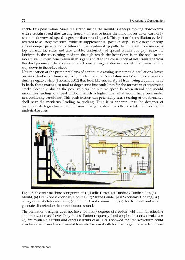
Fig. 1. Slab caster machine configuration: (1) Ladle Turret, (2) Tundish/Tundish Car, (3) Mould, (4) First Zone (Secondary Cooling), (5) Strand Guide (plus Secondary Cooling), (6) Straightener Withdrawal Units, (7) Dummy bar disconnect roll, (8) Torch cut-off unit – to generate discrete slabs from continuous strand.
The oscillation designer does not have too many degrees of freedom with him for effecting an optimization as above. Only the oscillation frequency f and amplitude a or s (stroke; s =
2a) are available. Suzuki and others (Suzuki et al., 1991) showed that the waveform could also be varied from the sinusoidal towards the saw-tooth form with gainful effects. Slower
www.intechopen.com
Optimization of Oscillation Parameters in Continuous Casting Process of Steel Manufacturing: Genetic Algorithms versus Differential Evolution
79
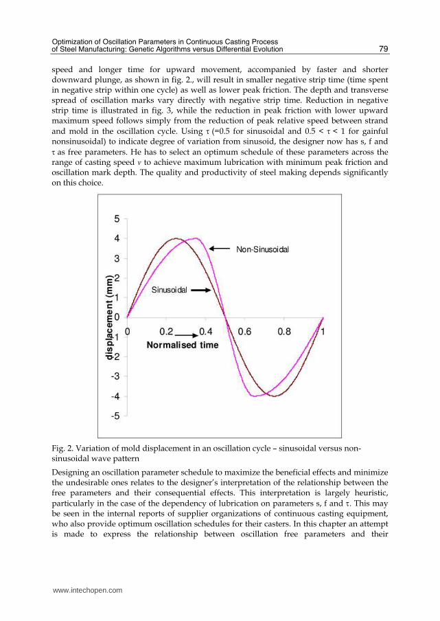
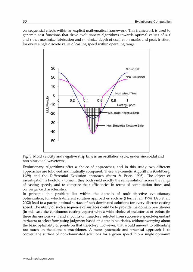
speed and longer time for upward movement, accompanied by faster and shorter downward plunge, as shown in fig. 2., will result in smaller negative strip time (time spent in negative strip within one cycle) as well as lower peak friction. The depth and transverse spread of oscillation marks vary directly with negative strip time. Reduction in negative strip time is illustrated in fig. 3, while the reduction in peak friction with lower upward maximum speed follows simply from the reduction of peak relative speed between strand
and mold in the oscillation cycle. Using τ (=0.5 for sinusoidal and 0.5 < τ < 1 for gainful nonsinusoidal) to indicate degree of variation from sinusoid, the designer now has s, f and
τ as free parameters. He has to select an optimum schedule of these parameters across the range of casting speed v to achieve maximum lubrication with minimum peak friction and oscillation mark depth. The quality and productivity of steel making depends significantly on this choice.
Fig. 2. Variation of mold displacement in an oscillation cycle – sinusoidal versus non-sinusoidal wave pattern
Designing an oscillation parameter schedule to maximize the beneficial effects and minimize the undesirable ones relates to the designer’s interpretation of the relationship between the free parameters and their consequential effects. This interpretation is largely heuristic,
particularly in the case of the dependency of lubrication on parameters s, f and τ. This may be seen in the internal reports of supplier organizations of continuous casting equipment, who also provide optimum oscillation schedules for their casters. In this chapter an attempt is made to express the relationship between oscillation free parameters and their
www.intechopen.com
Evolutionary Computation
80
consequential effects within an explicit mathematical framework. This framework is used to generate cost functions that drive evolutionary algorithms towards optimal values of s, f
and τ that maximize lubrication and minimize depth of oscillation marks and peak friction, for every single discrete value of casting speed within operating range.
Fig. 3. Mold velocity and negative strip time in an oscillation cycle, under sinusoidal and non-sinusoidal waveforms.
Evolutionary Algorithms offer a choice of approaches, and in this study two different approaches are followed and mutually compared. These are Genetic Algorithms (Goldberg, 1989) and the Differential Evolution approach (Storn & Price, 1995). The object of investigation is twofold – to see if they both yield exactly the same solution across the range of casting speeds, and to compare their efficiencies in terms of computation times and convergence characteristics. In principle this problem lies within the domain of multi-objective evolutionary optimization, for which different solution approaches such as (Horn et al., 1994; Deb et al., 2002) lead to a pareto-optimal surface of non-dominated solutions for every discrete casting speed. The utility of such a sequence of surfaces could be to provide the domain practitioner (in this case the continuous casting expert) with a wide choice of trajectories of points (in
three dimensions – s, f and τ; points on trajectory selected from successive speed-dependant surfaces) to select from using judgment based on domain heuristics, without worrying about the basic optimality of points on that trajectory. However, that would amount to offloading too much on the domain practitioner. A more systematic and practical approach is to convert the surface of non-dominated solutions for a given speed into a single optimum
www.intechopen.com
Optimization of Oscillation Parameters in Continuous Casting Process of Steel Manufacturing: Genetic Algorithms versus Differential Evolution
81
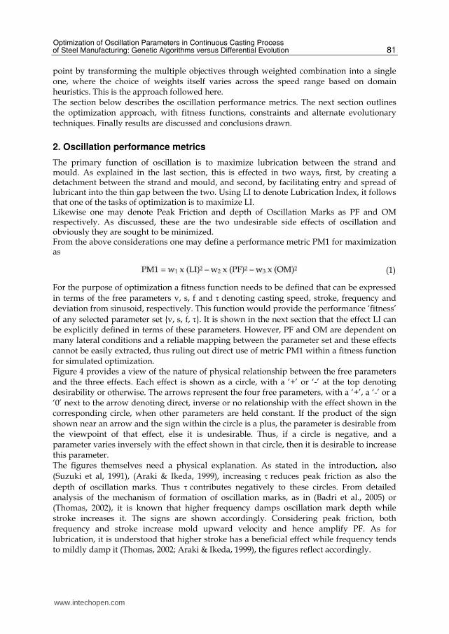
point by transforming the multiple objectives through weighted combination into a single one, where the choice of weights itself varies across the speed range based on domain heuristics. This is the approach followed here. The section below describes the oscillation performance metrics. The next section outlines the optimization approach, with fitness functions, constraints and alternate evolutionary techniques. Finally results are discussed and conclusions drawn.
2. Oscillation performance metrics
The primary function of oscillation is to maximize lubrication between the strand and mould. As explained in the last section, this is effected in two ways, first, by creating a detachment between the strand and mould, and second, by facilitating entry and spread of lubricant into the thin gap between the two. Using LI to denote Lubrication Index, it follows that one of the tasks of optimization is to maximize LI. Likewise one may denote Peak Friction and depth of Oscillation Marks as PF and OM respectively. As discussed, these are the two undesirable side effects of oscillation and obviously they are sought to be minimized. From the above considerations one may define a performance metric PM1 for maximization as
(1)
For the purpose of optimization a fitness function needs to be defined that can be expressed
in terms of the free parameters v, s, f and τ denoting casting speed, stroke, frequency and deviation from sinusoid, respectively. This function would provide the performance ‘fitness’
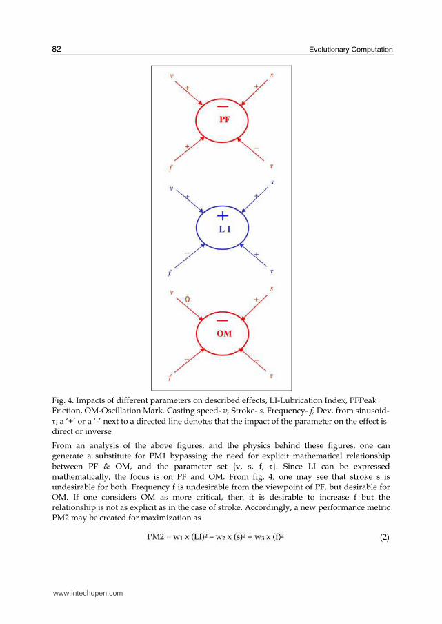
of any selected parameter set {v, s, f, τ}. It is shown in the next section that the effect LI can be explicitly defined in terms of these parameters. However, PF and OM are dependent on many lateral conditions and a reliable mapping between the parameter set and these effects cannot be easily extracted, thus ruling out direct use of metric PM1 within a fitness function for simulated optimization. Figure 4 provides a view of the nature of physical relationship between the free parameters and the three effects. Each effect is shown as a circle, with a ‘+’ or ‘-’ at the top denoting desirability or otherwise. The arrows represent the four free parameters, with a ‘+’, a ‘-’ or a ‘0’ next to the arrow denoting direct, inverse or no relationship with the effect shown in the corresponding circle, when other parameters are held constant. If the product of the sign shown near an arrow and the sign within the circle is a plus, the parameter is desirable from the viewpoint of that effect, else it is undesirable. Thus, if a circle is negative, and a parameter varies inversely with the effect shown in that circle, then it is desirable to increase this parameter. The figures themselves need a physical explanation. As stated in the introduction, also
(Suzuki et al, 1991), (Araki & Ikeda, 1999), increasing τ reduces peak friction as also the
depth of oscillation marks. Thus τ contributes negatively to these circles. From detailed analysis of the mechanism of formation of oscillation marks, as in (Badri et al., 2005) or (Thomas, 2002), it is known that higher frequency damps oscillation mark depth while stroke increases it. The signs are shown accordingly. Considering peak friction, both frequency and stroke increase mold upward velocity and hence amplify PF. As for lubrication, it is understood that higher stroke has a beneficial effect while frequency tends to mildly damp it (Thomas, 2002; Araki & Ikeda, 1999), the figures reflect accordingly.
www.intechopen.com
Evolutionary Computation
82
Fig. 4. Impacts of different parameters on described effects, LI-Lubrication Index, PFPeak Friction, OM-Oscillation Mark. Casting speed- v, Stroke- s, Frequency- f, Dev. from sinusoid-
τ; a ‘+’ or a ‘-’ next to a directed line denotes that the impact of the parameter on the effect is direct or inverse
From an analysis of the above figures, and the physics behind these figures, one can generate a substitute for PM1 bypassing the need for explicit mathematical relationship
between PF & OM, and the parameter set {v, s, f, τ}. Since LI can be expressed mathematically, the focus is on PF and OM. From fig. 4, one may see that stroke s is undesirable for both. Frequency f is undesirable from the viewpoint of PF, but desirable for OM. If one considers OM as more critical, then it is desirable to increase f but the relationship is not as explicit as in the case of stroke. Accordingly, a new performance metric PM2 may be created for maximization as
(2)
www.intechopen.com
Optimization of Oscillation Parameters in Continuous Casting Process of Steel Manufacturing: Genetic Algorithms versus Differential Evolution
83
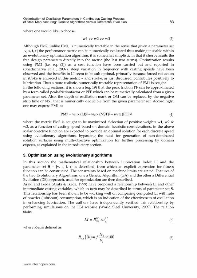
where one would like to choose
(3)
Although PM2, unlike PM1, is numerically tractable in the sense that given a parameter set
{v, s, f, τ} the performance metric can be numerically evaluated thus making it usable within an evolutionary optimization algorithm, it is somewhat simplistic in that it short-circuits the free design parameters directly into the metric (the last two terms). Optimization results using PM2 (i.e. eq. (2)) as a cost function have been carried out and reported in (Bhattacharya et al., 2007), steep variation in frequency with casting speeds have been observed and the benefits in LI seem to be sub-optimal, primarily because forced reduction in stroke is enforced in this metric – and stroke, as just discussed, contributes positively to lubrication. Thus a more realistic, numerically tractable representation of PM1 is sought. In the following sections, it is shown (eq. 19) that the peak friction PF can be approximated by a term called peak-frictionfactor or PFF which can be numerically calculated from a given parameter set. Also, the depth of oscillation mark or OM can be replaced by the negative strip time or NST that is numerically deducible from the given parameter set. Accordingly, one may express PM1 as
(4)
where the metric PM3 is sought to be maximized. Selection of positive weights w1, w2 & w3, as a function of casting speed based on domain-heuristic considerations, in the above scalar objective function are expected to provide an optimal solution for each discrete speed using evolutionary algorithms, bypassing the need for generation of non-dominated solution surfaces using multi-objective optimization for further processing by domain experts, as explained in the introductory section.
3. Optimization using evolutionary algorithms
In this section the mathematical relationship between Lubrication Index LI and the parameter set S = {v, s, f, τ} is described, from which an explicit expression for fitness function can be constructed. The constraints based on machine limits are stated. Features of the two Evolutionary Algorithms, one a Genetic Algorithm (GA) and the other a Differential Evolution (DE) approach, used for optimization are then described. Araki and Ikeda (Araki & Ikeda, 1999) have proposed a relationship between LI and other intermediate casting variables, which in turn may be described in terms of parameter set S. This relationship has been shown to be working well on comparing computed LI with rate of powder (lubricant) consumption, which is an indication of the effectiveness of oscillation in enhancing lubrication. The authors have independently verified this relationship by performing simulations on the IISI website (World Steel University, 2009). The relation states
(5)
where RNA is defined as
(6)
www.intechopen.com
Evolutionary Computation
84
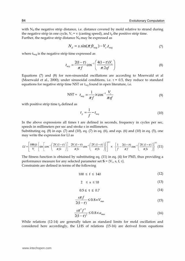
with Nd the negative strip distance, i.e. distance covered by mold relative to strand during the negative strip in one cycle, Vc = v (casting speed), and tp the positive strip time. Further, the negative strip distance Nd may be expressed as
(7)
where tneg is the negative strip time expressed as
(8)
Equations (7) and (8) for non-sinusoidal oscillations are according to Moerwald et al
(Moerwald et al., 2000); under sinusoidal conditions, i.e. τ = 0.5, they reduce to standard equations for negative strip time NST or tneg found in open literature, i.e.
(9)
with positive strip time tp defined as
(10)
In the above expressions all times t are defined in seconds, frequency in cycles per sec, speeds in millimeters per sec and stroke s in millimeters. Substituting eq. (8) in eqs. (7) and (10), eq. (7) in eq. (6), and eqs. (6) and (10) in eq. (5), one may write the expression for LI as
(11)
The fitness function is obtained by substituting eq. (11) in eq. (4) for PM3, thus providing a
performance measure for any selected parameter set S = {Vc, s, f, τ}. Constraints are defined in terms of the following
(12)
(13)
(14)
(15)
(16)
While relations (12-14) are generally taken as standard limits for mold oscillation and considered here accordingly, the LHS of relations (15-16) are derived from equations
www.intechopen.com
Optimization of Oscillation Parameters in Continuous Casting Process of Steel Manufacturing: Genetic Algorithms versus Differential Evolution
85
describing non-sinusoidal waveforms and correspond to the maximum attainable values of mold velocity and acceleration for a selected waveform. These are derived in Appendix A. Vmax and amax in the equations represent machine limits of velocity and acceleration provided by the equipment manufacturers. At a given value of v (=Vc), the peak friction PF may be expressed as
(17)
where is the maximum upward speed in a cycle, η is the viscosity of lubricant and dt
the thickness of lubricant film in the gap between strand and mould. The latter two being extraneous factors to an oscillation schedule, a Peak Friction Factor PFF may be defined such that
(18)
with
(19)
and
An Evolutionary Algorithm is used to derive that parameter set S which maximizes the
fitness function defined by performance metric PM3. In this process the casting speed v is
fixed, and s, f, and τ are evaluated as a function of v. Different values of v are fed as input,
the evolutionary algorithm generates corresponding optimal sets of s, f and τ.
As stated earlier, two alternate evolutionary algorithms are used competitively in this study and their results and performances assessed. Genetic Algorithms (GA) constitute the original method to have been developed in the field of evolutionary algorithms, and represent the baseline for further advances in this field. A standard GA process is well
known and not described here. The parameters to be optimized, namely s, f, and τ, are binary coded and concatenated to form bit strings (chromosomes) that constitute the population members operated upon in parallel. Each of the parameters are encoded using 10 bits, which implies that their respective ranges of variation, eqs. (12-14), are discretized into 1024 intervals, and that each chromosome is 30 bits long. In every generation the fitness of a population member is evaluated by calling the fitness function, expressed as eq. (4), the components of (4) provided by eqs. (9), (11) & (19). Genetic Algorithms tend to slow down after nearing an optimum solution point in the n-dimensional (here n = 3) solution space, and some means are usually implemented for accelerating the GA process. The acceleration methods used here are, first, elitism (Bhandari et al., 1996) where the best solution obtained in a certain generation is preserved in succeeding generations until a better one is found thus preventing ‘loss’ of good solutions, second, cyclical variation of mutation rate across generations (Pal et al., 1998), and third, differential mutation of bits according to significance in good and bad schema in solution strings (Bhattacharya & Sivakumar, 2000; Bhattacharya et al., 2004). The method of Differential Evolution (DE) was first proposed by Storn and Price (1995) and differs from GA primarily in the manner in which population members (i.e. solution parameter vectors) in a candidate solution pool are varied to create new solutions, and thus explore the solution space for the global optimum. In fact, most evolutionary optimization
www.intechopen.com
Evolutionary Computation
86
techniques fundamentally differ from one another in the manner of inducing variation in candidate solutions. GA’s use crossover between randomly selected solution pairs, and also mutation, to create new solutions. Differential Evolution, on the other hand, modifies a candidate solution by first creating a trial vector from three other solution vectors simply by adding the weighted vector difference of two of these to the third, and then operating a crossover between the trial vector and the original candidate solution to yield the new candidate. In the last step it follows the “greedy” approach, i.e. the newly generated solution replaces the original only if its fitness value is better. Expressed mathematically, a trial vector for a candidate i in a pool of size N at
generation g is created as
(20)
where r1, r2, r3 ∈ [0, N-1]; are integers and different from one another and from i, and F is a damping factor usually between 0.5 and 1.
Crossover is then executed between and the original candidate to yield the potential
new candidate solution which is allowed to replace the original only if its fitness value is found to be better. The actual implementation in this study is a variant of eq. (20) for generating the trial vector, on the lines of Karaboga and Ogdem (2004), and is expressed as
(21)
where the subscript best represent the vector having best fitness value in the population at generation g, and R is set at 0.5 while F varies randomly with generation g (constant across all i in a generation) within the range -2 to +2. The probability of crossover is set at 0.7, the same value as used in the GA.
4. Results and discussion
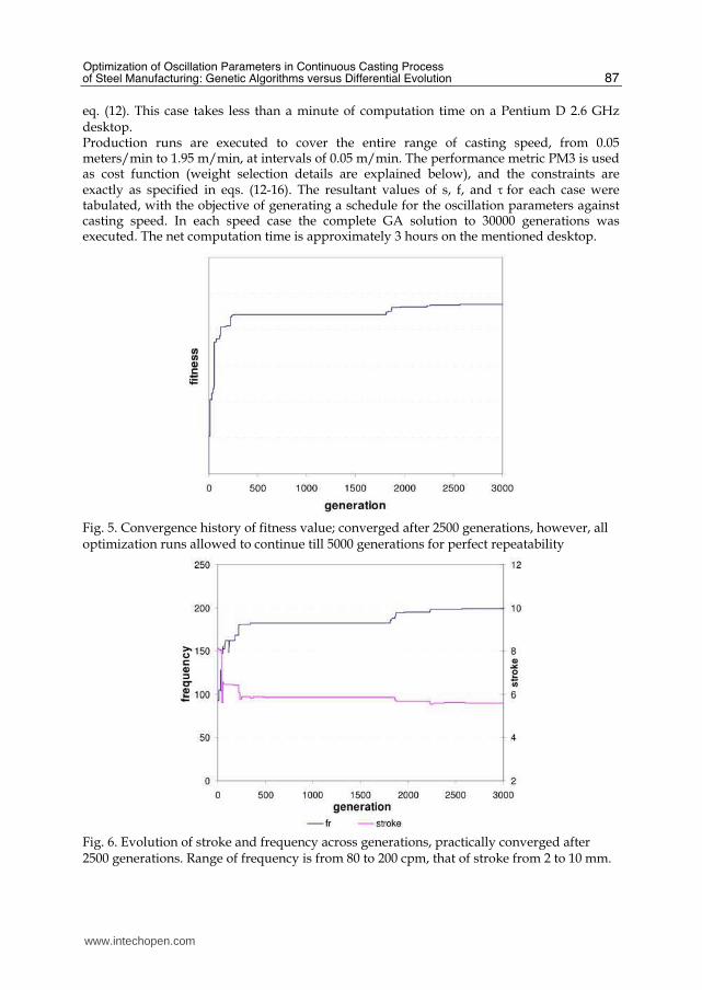
Evolutionary Algorithms as described above are used to optimize the oscillation parameters stroke, frequency and waveform (deviation from sinusoid), with the objective of maximizing lubrication and minimizing peak friction and oscillation marks. This is achieved by optimizing the fitness function according to eqs. (4), (9), (11) & (19), under the constraints expressed in relations (12-16). The results obtained from Genetic Algorithm are first described in detail. Next the results from Differential Evolution are shown in comparison to those obtained applying the GA approach. The GA is tested with different population sizes and a size of 20 is selected for performing downstream executions. A test case with w1 = 0.85, w2 = 0.13 and w3 = 0.02 (refer eq. 2) is taken at speed v = 1.4, and the variation of convergence history and final converged solution with arbitrary changes in initial population is observed. The objective function PM2 (eq. (2)) is used, and the solution is stopped after 5000 generations, a stage when it is assumed to have fully converged. Variations in convergence are seen only within the first 1000 generations; the final solution is always same with practically no variation. The convergence history is shown in figs. 5 & 6 for this test case, fig. 5 shows convergence of fitness function, and fig. 6 the evolution of stroke and frequency for first 3000 generations. In these test cases frequency is allowed to vary between 80 to 200, which is a wider range than that specified in
www.intechopen.com
Optimization of Oscillation Parameters in Continuous Casting Process of Steel Manufacturing: Genetic Algorithms versus Differential Evolution
87
eq. (12). This case takes less than a minute of computation time on a Pentium D 2.6 GHz desktop. Production runs are executed to cover the entire range of casting speed, from 0.05 meters/min to 1.95 m/min, at intervals of 0.05 m/min. The performance metric PM3 is used as cost function (weight selection details are explained below), and the constraints are exactly as specified in eqs. (12-16). The resultant values of s, f, and τ for each case were tabulated, with the objective of generating a schedule for the oscillation parameters against casting speed. In each speed case the complete GA solution to 30000 generations was executed. The net computation time is approximately 3 hours on the mentioned desktop.
Fig. 5. Convergence history of fitness value; converged after 2500 generations, however, all optimization runs allowed to continue till 5000 generations for perfect repeatability
Fig. 6. Evolution of stroke and frequency across generations, practically converged after 2500 generations. Range of frequency is from 80 to 200 cpm, that of stroke from 2 to 10 mm.
www.intechopen.com
Evolutionary Computation
88
Referring back to the discussion on Oscillation Performance Metric 3 (PM3, eq. (4)), the oscillation schedule designer would like to arrange the weights w1, w2 & w3 given to LI, NST and PFF in a manner consistent with his understanding /interpretation of domain heuristics. The three weights should preferably add up to one to normalize different weight allocation strategies. Facilitating lubrication being the prime purpose of oscillations, prima-facie the major share of weight should be allocated to LI (i.e. w1). Between NST and PFF, one may say that NST is more important as it can directly affect product quality while the latter can be somewhat compensated with higher LI. Thus, one may broadly set an inequality of the form
(22)
Now, for a class of steels called “peritectic” primarily on the basis of their carbon
concentration, oscillation marks and their consequential effects are of greater concern than
in case of low or medium carbon grades. Correspondingly, the LI is of a slightly lower
concern in peritectic grades. (Figures (9-10) showing variation of LI and NST with casting
speed as calculated from oscillation schedules provided by an OEM (Original Equipment
Manufacturer), for peritectic and low/mid-C grades, corroborate this relative prioritization
of oscillation performance objectives across steel grades. These figures also show GA results
on which we are not focusing right here, but will return to later for discussion). Thus,
between w1 and w2 (weights of LI and NST), the designer’s preference is for higher
difference (w1 – w2) for low/mid Carbon steels as compared to peritectic. Also, this
difference should increase with casting speeds, to offset lower LI at higher speeds and
deeper oscillation marks at lower speeds.
From the above discussions the following requirements can be defined on the selection of
weights w1, w2 & w3. First,
Second, difference D = (w1 – w2) should be greater in the case of low/mid-C as compared to peritectic grades. Third, D should be gradually increasing with casting speeds. Based on the above requirements, the following pattern of variation of weights was implemented: For peritectic grades:
Case (a) w1 = 0.6, w2 = 0.3, w3 = 0.1; for cs ≤ 0.8 m/min.; cs denotes casting speed
Case (b) w1 = 0.7, w2 = 0.2, w3 = 0.1; for cs ≥ 1.4, and Case (c) w1 and w2 vary linearly from case (a) to (b) for 0.8 < cs < 1.4. For low- and mid- C grades:
Case (a) w1 = 0.6, w2 = 0.3, w3 = 0.1; for cs ≤ 0.8 m/min.
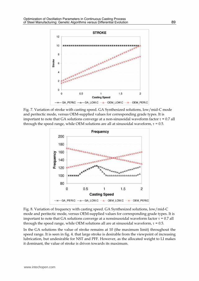
Case (b) w1 = 0.85, w2 = 0.075, w3 = 0.075; for cs ≥ 1.4, and Case (c) w1, w2 and w3 vary linearly from case (a) to (b) for 0.8 < cs < 1.4. Figures 7 and 8 show variation of stroke and frequency, respectively, with casting speed for the two GA solutions against the schedules provided by the Original Equipment Manufacturer (OEM) for the same two grade cases. The value of deviationfrom-sinusoid
τ quickly converges to the maximum (0.7) and hardly moves from there across the speed
range, and hence this is not plotted. Recall from fig. 4 that increased τ was desirable from the perspective of all 3 effects, and the GA solutions strongly confirm this. One needs to
keep in mind that both OEM schedules are provided at sinusoidal waveform, i.e. τ = 0.5.
www.intechopen.com
Optimization of Oscillation Parameters in Continuous Casting Process of Steel Manufacturing: Genetic Algorithms versus Differential Evolution
89
Fig. 7. Variation of stroke with casting speed. GA Synthesized solutions, low/mid-C mode and peritectic mode, versus OEM-supplied values for corresponding grade types. It is
important to note that GA solutions converge at a non-sinusoidal waveform factor τ = 0.7 all
through the speed range, while OEM solutions are all at sinusoidal waveform, τ = 0.5.
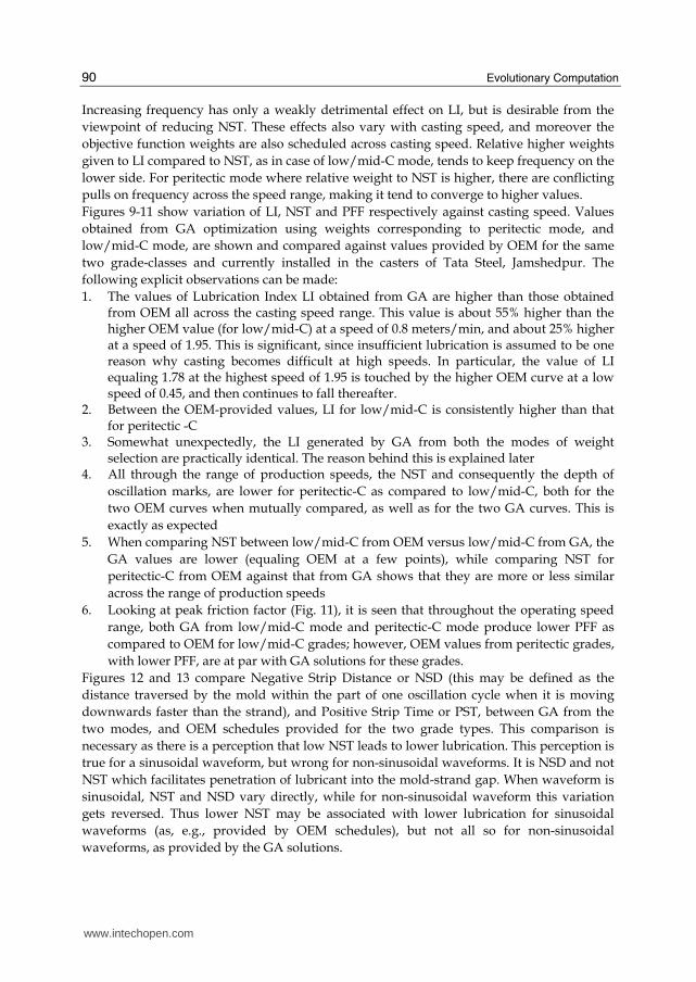
Fig. 8. Variation of frequency with casting speed. GA Synthesized solutions, low/mid-C mode and peritectic mode, versus OEM-supplied values for corresponding grade types. It is
important to note that GA solutions converge at a nonsinusoidal waveform factor τ = 0.7 all
through the speed range, while OEM solutions all are at sinusoidal waveform, τ = 0.5.
In the GA solutions the value of stroke remains at 10 (the maximum limit) throughout the speed range. It is seen in fig. 4. that large stroke is desirable from the viewpoint of increasing lubrication, but undesirable for NST and PFF. However, as the allocated weight to LI makes it dominant, the value of stroke is driven towards its maximum.
www.intechopen.com
Evolutionary Computation
90
Increasing frequency has only a weakly detrimental effect on LI, but is desirable from the
viewpoint of reducing NST. These effects also vary with casting speed, and moreover the
objective function weights are also scheduled across casting speed. Relative higher weights
given to LI compared to NST, as in case of low/mid-C mode, tends to keep frequency on the
lower side. For peritectic mode where relative weight to NST is higher, there are conflicting
pulls on frequency across the speed range, making it tend to converge to higher values.
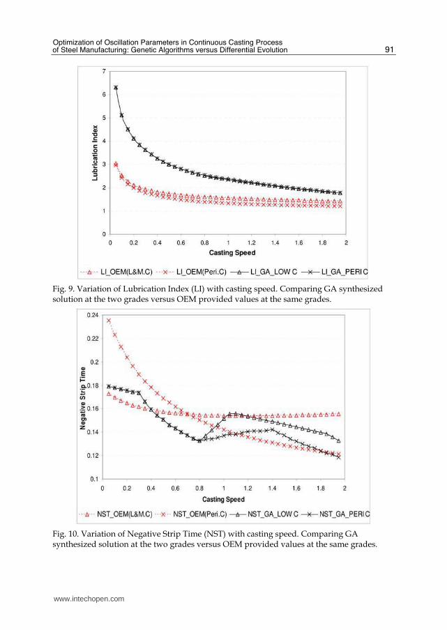
Figures 9-11 show variation of LI, NST and PFF respectively against casting speed. Values
obtained from GA optimization using weights corresponding to peritectic mode, and
low/mid-C mode, are shown and compared against values provided by OEM for the same
two grade-classes and currently installed in the casters of Tata Steel, Jamshedpur. The
following explicit observations can be made:
1. The values of Lubrication Index LI obtained from GA are higher than those obtained from OEM all across the casting speed range. This value is about 55% higher than the higher OEM value (for low/mid-C) at a speed of 0.8 meters/min, and about 25% higher at a speed of 1.95. This is significant, since insufficient lubrication is assumed to be one reason why casting becomes difficult at high speeds. In particular, the value of LI equaling 1.78 at the highest speed of 1.95 is touched by the higher OEM curve at a low speed of 0.45, and then continues to fall thereafter.
2. Between the OEM-provided values, LI for low/mid-C is consistently higher than that for peritectic -C
3. Somewhat unexpectedly, the LI generated by GA from both the modes of weight selection are practically identical. The reason behind this is explained later
4. All through the range of production speeds, the NST and consequently the depth of
oscillation marks, are lower for peritectic-C as compared to low/mid-C, both for the
two OEM curves when mutually compared, as well as for the two GA curves. This is
exactly as expected
5. When comparing NST between low/mid-C from OEM versus low/mid-C from GA, the
GA values are lower (equaling OEM at a few points), while comparing NST for
peritectic-C from OEM against that from GA shows that they are more or less similar
across the range of production speeds
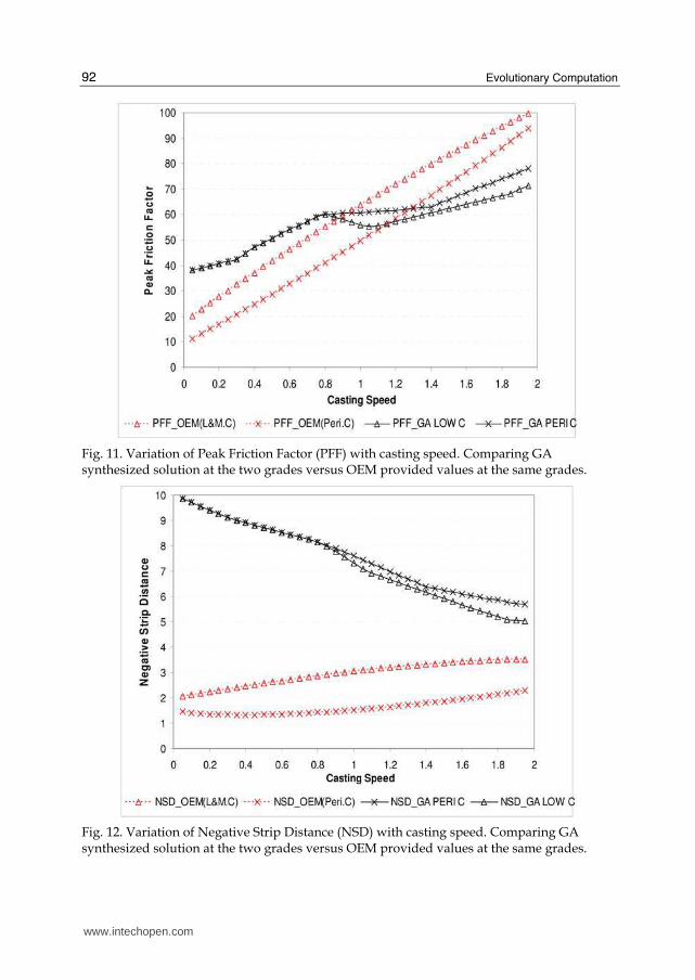
6. Looking at peak friction factor (Fig. 11), it is seen that throughout the operating speed
range, both GA from low/mid-C mode and peritectic-C mode produce lower PFF as
compared to OEM for low/mid-C grades; however, OEM values from peritectic grades,
with lower PFF, are at par with GA solutions for these grades.
Figures 12 and 13 compare Negative Strip Distance or NSD (this may be defined as the
distance traversed by the mold within the part of one oscillation cycle when it is moving
downwards faster than the strand), and Positive Strip Time or PST, between GA from the
two modes, and OEM schedules provided for the two grade types. This comparison is
necessary as there is a perception that low NST leads to lower lubrication. This perception is
true for a sinusoidal waveform, but wrong for non-sinusoidal waveforms. It is NSD and not
NST which facilitates penetration of lubricant into the mold-strand gap. When waveform is
sinusoidal, NST and NSD vary directly, while for non-sinusoidal waveform this variation
gets reversed. Thus lower NST may be associated with lower lubrication for sinusoidal
waveforms (as, e.g., provided by OEM schedules), but not all so for non-sinusoidal
waveforms, as provided by the GA solutions.
www.intechopen.com
Optimization of Oscillation Parameters in Continuous Casting Process of Steel Manufacturing: Genetic Algorithms versus Differential Evolution
91
Fig. 9. Variation of Lubrication Index (LI) with casting speed. Comparing GA synthesized solution at the two grades versus OEM provided values at the same grades.
Fig. 10. Variation of Negative Strip Time (NST) with casting speed. Comparing GA synthesized solution at the two grades versus OEM provided values at the same grades.
www.intechopen.com
Evolutionary Computation
92
Fig. 11. Variation of Peak Friction Factor (PFF) with casting speed. Comparing GA synthesized solution at the two grades versus OEM provided values at the same grades.
Fig. 12. Variation of Negative Strip Distance (NSD) with casting speed. Comparing GA synthesized solution at the two grades versus OEM provided values at the same grades.
www.intechopen.com
Optimization of Oscillation Parameters in Continuous Casting Process of Steel Manufacturing: Genetic Algorithms versus Differential Evolution
93
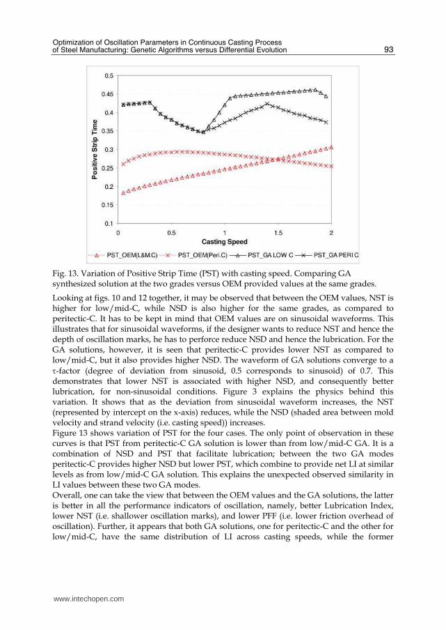
Fig. 13. Variation of Positive Strip Time (PST) with casting speed. Comparing GA synthesized solution at the two grades versus OEM provided values at the same grades.
Looking at figs. 10 and 12 together, it may be observed that between the OEM values, NST is higher for low/mid-C, while NSD is also higher for the same grades, as compared to peritectic-C. It has to be kept in mind that OEM values are on sinusoidal waveforms. This illustrates that for sinusoidal waveforms, if the designer wants to reduce NST and hence the depth of oscillation marks, he has to perforce reduce NSD and hence the lubrication. For the GA solutions, however, it is seen that peritectic-C provides lower NST as compared to low/mid-C, but it also provides higher NSD. The waveform of GA solutions converge to a
τ-factor (degree of deviation from sinusoid, 0.5 corresponds to sinusoid) of 0.7. This demonstrates that lower NST is associated with higher NSD, and consequently better lubrication, for non-sinusoidal conditions. Figure 3 explains the physics behind this variation. It shows that as the deviation from sinusoidal waveform increases, the NST (represented by intercept on the x-axis) reduces, while the NSD (shaded area between mold velocity and strand velocity (i.e. casting speed)) increases. Figure 13 shows variation of PST for the four cases. The only point of observation in these curves is that PST from peritectic-C GA solution is lower than from low/mid-C GA. It is a combination of NSD and PST that facilitate lubrication; between the two GA modes peritectic-C provides higher NSD but lower PST, which combine to provide net LI at similar levels as from low/mid-C GA solution. This explains the unexpected observed similarity in LI values between these two GA modes. Overall, one can take the view that between the OEM values and the GA solutions, the latter is better in all the performance indicators of oscillation, namely, better Lubrication Index, lower NST (i.e. shallower oscillation marks), and lower PFF (i.e. lower friction overhead of oscillation). Further, it appears that both GA solutions, one for peritectic-C and the other for low/mid-C, have the same distribution of LI across casting speeds, while the former
www.intechopen.com
Evolutionary Computation
94
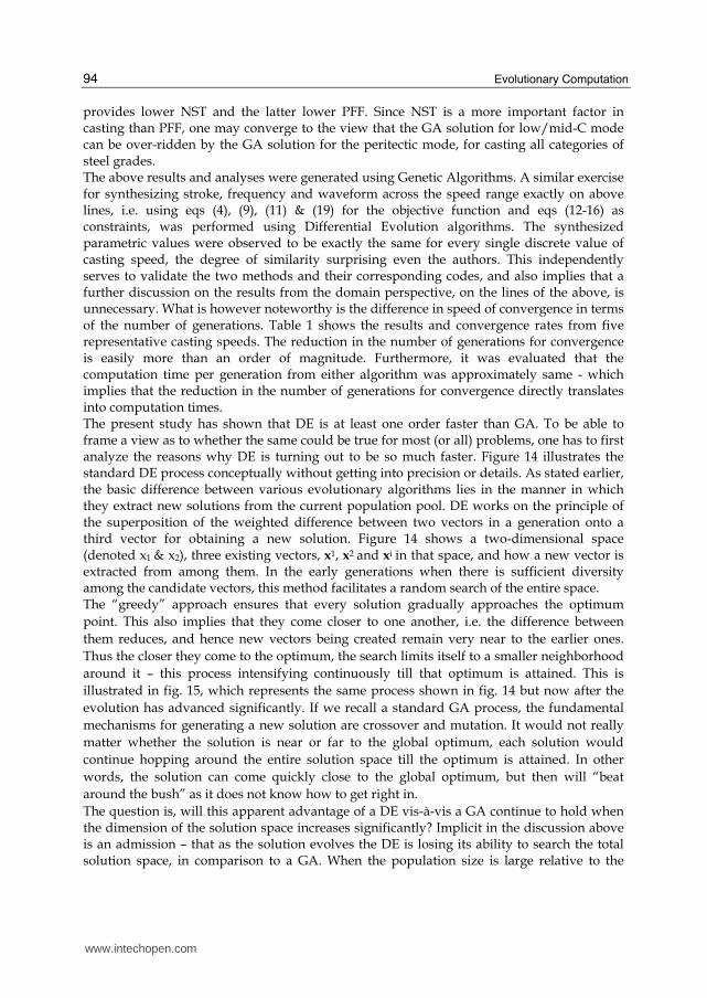
provides lower NST and the latter lower PFF. Since NST is a more important factor in casting than PFF, one may converge to the view that the GA solution for low/mid-C mode can be over-ridden by the GA solution for the peritectic mode, for casting all categories of steel grades. The above results and analyses were generated using Genetic Algorithms. A similar exercise for synthesizing stroke, frequency and waveform across the speed range exactly on above lines, i.e. using eqs (4), (9), (11) & (19) for the objective function and eqs (12-16) as constraints, was performed using Differential Evolution algorithms. The synthesized parametric values were observed to be exactly the same for every single discrete value of casting speed, the degree of similarity surprising even the authors. This independently serves to validate the two methods and their corresponding codes, and also implies that a further discussion on the results from the domain perspective, on the lines of the above, is unnecessary. What is however noteworthy is the difference in speed of convergence in terms of the number of generations. Table 1 shows the results and convergence rates from five representative casting speeds. The reduction in the number of generations for convergence is easily more than an order of magnitude. Furthermore, it was evaluated that the computation time per generation from either algorithm was approximately same - which implies that the reduction in the number of generations for convergence directly translates into computation times. The present study has shown that DE is at least one order faster than GA. To be able to frame a view as to whether the same could be true for most (or all) problems, one has to first analyze the reasons why DE is turning out to be so much faster. Figure 14 illustrates the standard DE process conceptually without getting into precision or details. As stated earlier, the basic difference between various evolutionary algorithms lies in the manner in which they extract new solutions from the current population pool. DE works on the principle of the superposition of the weighted difference between two vectors in a generation onto a third vector for obtaining a new solution. Figure 14 shows a two-dimensional space (denoted x1 & x2), three existing vectors, x1, x2 and xi in that space, and how a new vector is extracted from among them. In the early generations when there is sufficient diversity among the candidate vectors, this method facilitates a random search of the entire space. The “greedy” approach ensures that every solution gradually approaches the optimum
point. This also implies that they come closer to one another, i.e. the difference between
them reduces, and hence new vectors being created remain very near to the earlier ones.
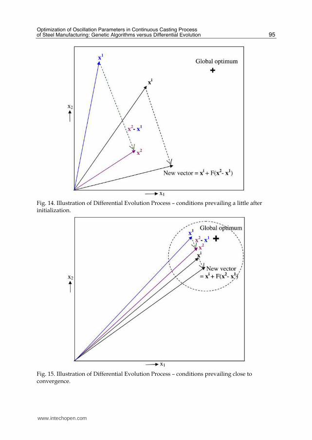
Thus the closer they come to the optimum, the search limits itself to a smaller neighborhood
around it – this process intensifying continuously till that optimum is attained. This is
illustrated in fig. 15, which represents the same process shown in fig. 14 but now after the
evolution has advanced significantly. If we recall a standard GA process, the fundamental
mechanisms for generating a new solution are crossover and mutation. It would not really
matter whether the solution is near or far to the global optimum, each solution would
continue hopping around the entire solution space till the optimum is attained. In other
words, the solution can come quickly close to the global optimum, but then will “beat
around the bush” as it does not know how to get right in.
The question is, will this apparent advantage of a DE vis-à-vis a GA continue to hold when the dimension of the solution space increases significantly? Implicit in the discussion above is an admission – that as the solution evolves the DE is losing its ability to search the total solution space, in comparison to a GA. When the population size is large relative to the
www.intechopen.com
Optimization of Oscillation Parameters in Continuous Casting Process of Steel Manufacturing: Genetic Algorithms versus Differential Evolution
95
Fig. 14. Illustration of Differential Evolution Process – conditions prevailing a little after initialization.
Fig. 15. Illustration of Differential Evolution Process – conditions prevailing close to convergence.
www.intechopen.com
Evolutionary Computation
96
parametric degrees of freedom, and the initial choice sufficiently diverse, the possibility of quickly reaching a neighborhood of the global optimum is also high. But under the opposite conditions, i.e. large dimensionality of solution space and relatively smaller population size and initial diversity, the DE can possibly get trapped in a local minimum unless certain mechanisms for diversity retention are built in. These very mechanisms will, however, affect convergence rates in the final stages. From the above discussion it appears that the best approach would be to use DE alone whenever it is possible to have a large population size relative to the dimension of the solution space. If this is not possible, then it is advisable to use GA in the initial stages and switch to DE later when convergence rates fall significantly.
Casting Speed
(m/min)
Stroke-GA
(mm)
Stroke – DE (mm)
Frequency-GA (cpm)
Frequency-DE (cpm)
Final Fitness-GA (Eq.
4)
Final Fitness – DE
(Eq. 4)
Number of
Generations-
GA
Number of
Generations-
DE
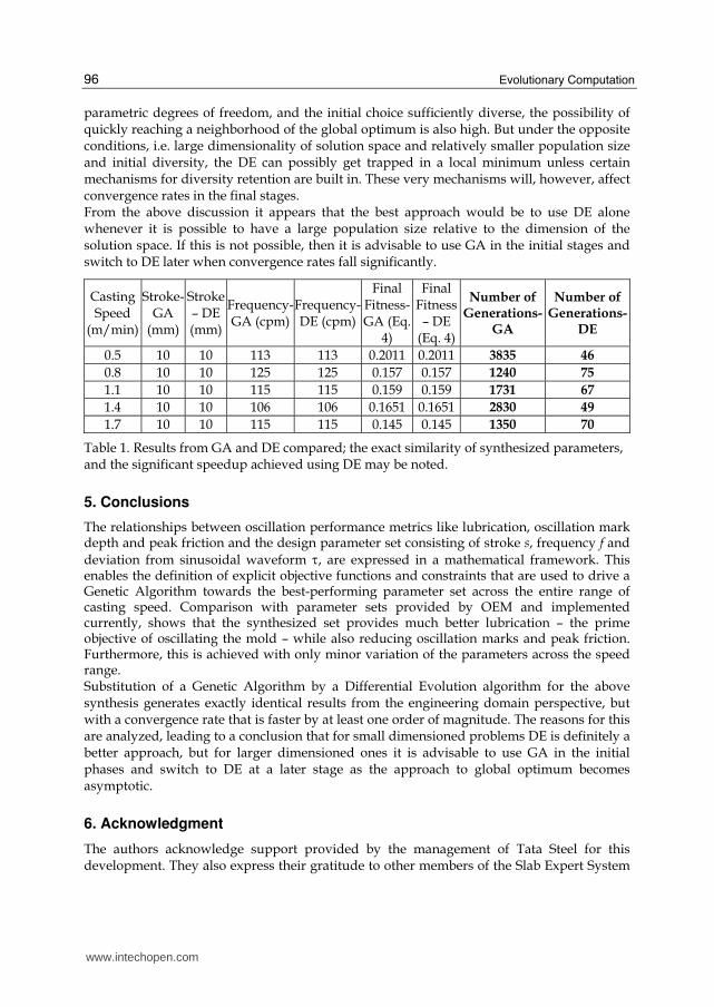
0.5 10 10 113 113 0.2011 0.2011 3835 46
0.8 10 10 125 125 0.157 0.157 1240 75
1.1 10 10 115 115 0.159 0.159 1731 67
1.4 10 10 106 106 0.1651 0.1651 2830 49
1.7 10 10 115 115 0.145 0.145 1350 70
Table 1. Results from GA and DE compared; the exact similarity of synthesized parameters, and the significant speedup achieved using DE may be noted.
5. Conclusions
The relationships between oscillation performance metrics like lubrication, oscillation mark depth and peak friction and the design parameter set consisting of stroke s, frequency f and
deviation from sinusoidal waveform τ, are expressed in a mathematical framework. This enables the definition of explicit objective functions and constraints that are used to drive a Genetic Algorithm towards the best-performing parameter set across the entire range of casting speed. Comparison with parameter sets provided by OEM and implemented currently, shows that the synthesized set provides much better lubrication – the prime objective of oscillating the mold – while also reducing oscillation marks and peak friction. Furthermore, this is achieved with only minor variation of the parameters across the speed range. Substitution of a Genetic Algorithm by a Differential Evolution algorithm for the above synthesis generates exactly identical results from the engineering domain perspective, but with a convergence rate that is faster by at least one order of magnitude. The reasons for this are analyzed, leading to a conclusion that for small dimensioned problems DE is definitely a better approach, but for larger dimensioned ones it is advisable to use GA in the initial phases and switch to DE at a later stage as the approach to global optimum becomes asymptotic.
6. Acknowledgment
The authors acknowledge support provided by the management of Tata Steel for this development. They also express their gratitude to other members of the Slab Expert System
www.intechopen.com
Optimization of Oscillation Parameters in Continuous Casting Process of Steel Manufacturing: Genetic Algorithms versus Differential Evolution
97
development team, members of the Flat Products Technology Group and continuous casting operations personnel for their support.
7. Appendix A: derivation of constraint equations on velocity and acceleration
The maximum values that stroke s, frequency f and waveform deviation from sinusoid τ can attain are limited not only by their range but the maximum velocity and acceleration that the mold can acquire within its oscillation cycle under the limiting conditions imposed by the machinery. These limits need to be converted into constraining equations for
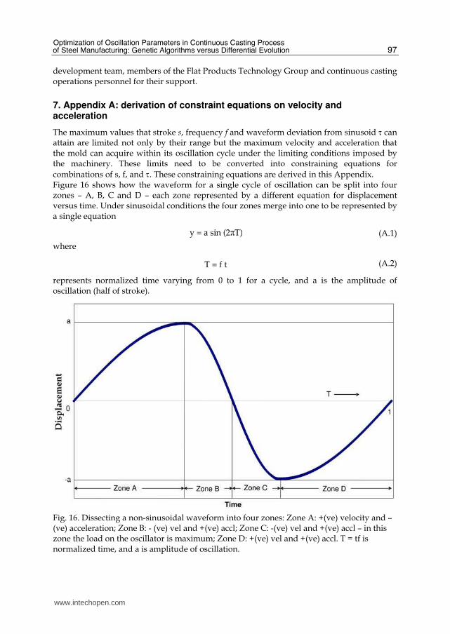
combinations of s, f, and τ. These constraining equations are derived in this Appendix. Figure 16 shows how the waveform for a single cycle of oscillation can be split into four zones – A, B, C and D – each zone represented by a different equation for displacement versus time. Under sinusoidal conditions the four zones merge into one to be represented by a single equation
(A.1)
where
(A.2)
represents normalized time varying from 0 to 1 for a cycle, and a is the amplitude of oscillation (half of stroke).
Fig. 16. Dissecting a non-sinusoidal waveform into four zones: Zone A: +(ve) velocity and –(ve) acceleration; Zone B: - (ve) vel and +(ve) accl; Zone C: -(ve) vel and +(ve) accl – in this zone the load on the oscillator is maximum; Zone D: +(ve) vel and +(ve) accl. T = tf is normalized time, and a is amplitude of oscillation.
www.intechopen.com
Evolutionary Computation
98
To obtain the velocity constraint equation, first the corresponding velocities versus time
equations are evaluated. The value of T at which they maximize is obtained by setting the
derivatives of these equations to zero and then solving for T. The expression for Tmax is
substituted back into the equation for velocity in the relevant zone to obtain the equation for
Vmax as a function of s, f, and τ. This provides the maximum attainable value of V for a given
combination of these parameters in one oscillation cycle. This expression is set to be less
than 80% of the manufacturer-provided machine limit for velocity, thus generating the
constraint equation (or inequation) for velocity.
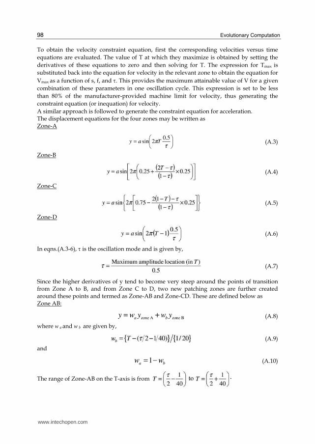
A similar approach is followed to generate the constraint equation for acceleration. The displacement equations for the four zones may be written as Zone-A
(A.3)
Zone-B
(A.4)
Zone-C
(A.5)
Zone-D
(A.6)
In eqns.(A.3-6), τ is the oscillation mode and is given by,
(A.7)
Since the higher derivatives of y tend to become very steep around the points of transition from Zone A to B, and from Zone C to D, two new patching zones are further created around these points and termed as Zone-AB and Zone-CD. These are defined below as Zone AB:
(A.8)
where w a and w b are given by,
(A.9)
and
(A.10)
The range of Zone-AB on the T-axis is from
www.intechopen.com
Optimization of Oscillation Parameters in Continuous Casting Process of Steel Manufacturing: Genetic Algorithms versus Differential Evolution
99
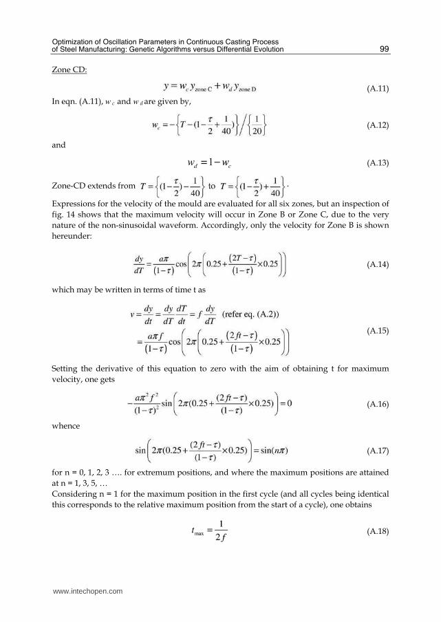
Zone CD:
(A.11)
In eqn. (A.11), w c and w d are given by,
(A.12)
and
(A.13)
Zone-CD extends from
Expressions for the velocity of the mould are evaluated for all six zones, but an inspection of
fig. 14 shows that the maximum velocity will occur in Zone B or Zone C, due to the very
nature of the non-sinusoidal waveform. Accordingly, only the velocity for Zone B is shown
hereunder:
(A.14)
which may be written in terms of time t as
(A.15)
Setting the derivative of this equation to zero with the aim of obtaining t for maximum
velocity, one gets
(A.16)
whence
(A.17)
for n = 0, 1, 2, 3 …. for extremum positions, and where the maximum positions are attained
at n = 1, 3, 5, …
Considering n = 1 for the maximum position in the first cycle (and all cycles being identical
this corresponds to the relative maximum position from the start of a cycle), one obtains
(A.18)
www.intechopen.com
Evolutionary Computation
100
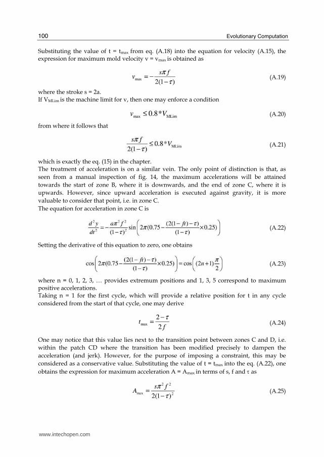
Substituting the value of t = tmax from eq. (A.18) into the equation for velocity (A.15), the expression for maximum mold velocity v = vmax is obtained as
(A.19)
where the stroke s = 2a. If VMLim is the machine limit for v, then one may enforce a condition
(A.20)
from where it follows that
(A.21)
which is exactly the eq. (15) in the chapter. The treatment of acceleration is on a similar vein. The only point of distinction is that, as
seen from a manual inspection of fig. 14, the maximum accelerations will be attained
towards the start of zone B, where it is downwards, and the end of zone C, where it is
upwards. However, since upward acceleration is executed against gravity, it is more
valuable to consider that point, i.e. in zone C.
The equation for acceleration in zone C is
(A.22)
Setting the derivative of this equation to zero, one obtains
(A.23)
where n = 0, 1, 2, 3, … provides extremum positions and 1, 3, 5 correspond to maximum positive accelerations. Taking n = 1 for the first cycle, which will provide a relative position for t in any cycle
considered from the start of that cycle, one may derive
(A.24)
One may notice that this value lies next to the transition point between zones C and D, i.e.
within the patch CD where the transition has been modified precisely to dampen the
acceleration (and jerk). However, for the purpose of imposing a constraint, this may be
considered as a conservative value. Substituting the value of t = tmax into the eq. (A.22), one
obtains the expression for maximum acceleration A = Amax in terms of s, f and τ as
(A.25)
www.intechopen.com

Optimization of Oscillation Parameters in Continuous Casting Process of Steel Manufacturing: Genetic Algorithms versus Differential Evolution
101
If AMLim is the machine limit for A, then one may enforce a condition
(A.26)
whence
(A.27)
which is exactly the eq. (16) in the chapter.
8. References
Araki, T. & Ikeda, M. (1999). Optimization Of Mould Oscillation For High Speed Casting–New Criteria For Mould Oscillation. Canadian Metallurgical Quarterly, Vol 38, No. 5., 1999, pp. 295-300.
Badri, A., et al. (2005). A Mold Simulator for Continuous Casting of Steel: Part II. The Formation of Oscillation Marks during the Continuous Casting of Low Carbon Steel. Metallurgical and Materials Transactions, Vol. 36B, June 2005, pp. 373- 383.
Bhattacharya, A.K. & Sivakumar, A.K. (2000). Design of Fuzzy Logic Controller for unstable fighter aircraft using a Genetic Algorithm for rule optimization. AIAA Guidance, Navigation and Control Conference, (Denver) August 2000, AIAA Paper 2000-4278.
Bhattacharya, A.K.; Kumar, J. & Jayati, P. (2004). Optimal routing of concurrent vehicles in a minefield using Genetic Algorithms. Tata Search Vol. 2, 2004, pp. 436-442.
Bhattacharya, A.K.; Debjani, S.; RoyChoudhury, A. & Das, J. (2007). Optimization of Continuous Casting Mould Oscillation Parameters in Steel Manufacturing Process using Genetic Algorithms. Proceedings of 2007 IEEE Congress on Evolutionary Computation.
Bhandari, D.; Murthy, C.A. & Pal, S.K. (1996). Genetic Algorithm with Elitist Model and its Convergence. Int. J. PatternRecognition and Artificial Intelligence, Vol.10, 1996, pp. 731-747.
Deb, K.; Agrawal, S.; Pratap, A. & Meyarivan, T. (2002). A fast and elitist multi-objective genetic algorithm: NSGA-II. IEEE Transactions on Evolutionary Computation, 6(2): 182-197, 2002.
Goldberg, D. E. (1989). Genetic Algorithms in Search, Optimization, and Machine Learning, Addison-Wesley Professional, ISBN 978-0201157673.
Horn, J.; Nafpliotis, N. & Goldberg, D.E. (1994). A niched Pareto Genetic Algorithm for multiobjective optimization. Proceedings of 1st IEEE Conf. on Evolutionary Computation, Vol 1, 1994, pp. 82-87.
Karaboga, D. & Okdem, S. (2004). A simple and global optimization algorithm for engineering problems: Differential Evolution Algorithm. Turkish J. Elec Engg. Vol. 12, No. 1, 2004, pp. 53-60.
Moerwald, K.; Steinrueck, H. & Rudischer, C. (2000). Theoretical Studies to Adjust Proper Mould Oscillation Parameters. AIST Conference 2000.
Pal, S.K.; Bandopadhyay, S. & Murthy, C.A. (1998). Genetic Algorithms for generation of Class Boundaries. IEEE Trans. On Systems, Man and Cybernetics¾ Part B: Cybernetics, Vol. 28, No. 6, December 1998, pp. 816-828.
www.intechopen.com
Evolutionary Computation
102
Storn, R. & Price, K. (1995). Differential Evolution – a simple and efficient adaptive scheme for global optimization over continuous spaces. ICSI Technical Report TR-95-012, March 1995.
Suzuki, M. et al. (1991). Development of a New Mould Oscillation Mode for High-speed Continuous Casting of Steel Slabs. ISIJ International, Vol 31, No. 3, 1991, pp. 254-261.
Thomas, B.G. (2002). Modelling of the Continuous Casting of Steel – Past, Present and Future. Electric Furnace Conf. Proc., Vol. 59, ISS, Warrendale, PA, (Phoenix, AZ), 2001, 3-30, also Metallurgical and Materials Transactions B, Vol 33B, No. 6, Dec 2002, pp. 795-812.
World Steel University site. (2009). Continuous casting link: http://www.steeluniversity.org/content/html/eng/default.asp?catid=27&pageid=2081271520
www.intechopen.com
Evolutionary ComputationEdited by Wellington Pinheiro dos Santos
ISBN 978-953-307-008-7Hard cover, 572 pagesPublisher InTechPublished online 01, October, 2009Published in print edition October, 2009
InTech EuropeUniversity Campus STeP Ri Slavka Krautzeka 83/A 51000 Rijeka, Croatia Phone: +385 (51) 770 447 Fax: +385 (51) 686 166www.intechopen.com
InTech ChinaUnit 405, Office Block, Hotel Equatorial Shanghai No.65, Yan An Road (West), Shanghai, 200040, China
Phone: +86-21-62489820 Fax: +86-21-62489821
This book presents several recent advances on Evolutionary Computation, specially evolution-basedoptimization methods and hybrid algorithms for several applications, from optimization and learning to patternrecognition and bioinformatics. This book also presents new algorithms based on several analogies andmetafores, where one of them is based on philosophy, specifically on the philosophy of praxis and dialectics. Inthis book it is also presented interesting applications on bioinformatics, specially the use of particle swarms todiscover gene expression patterns in DNA microarrays. Therefore, this book features representative work onthe field of evolutionary computation and applied sciences. The intended audience is graduate,undergraduate, researchers, and anyone who wishes to become familiar with the latest research work on thisfield.
How to referenceIn order to correctly reference this scholarly work, feel free to copy and paste the following:
Arya K. Bhattacharya and Debjani Sambasivam (2009). Optimization of Oscillation Parameters in ContinuousCasting Process of Steel Manufacturing: Genetic Algorithms versus Differential Evolution, EvolutionaryComputation, Wellington Pinheiro dos Santos (Ed.), ISBN: 978-953-307-008-7, InTech, Available from:http://www.intechopen.com/books/evolutionary-computation/optimization-of-oscillation-parameters-in-continuous-casting-process-of-steel-manufacturing-genetic-