Optimizare multiobiectiv utilizand algoritmi genetici ... · Optimizare multiobiectiv utilizand algoritmi genetici Multiobjective optimization using genetic algorithms

Optimizare multiobiectiv

utilizand

algoritmi genetici

Multiobjective optimization

using

genetic algorithms

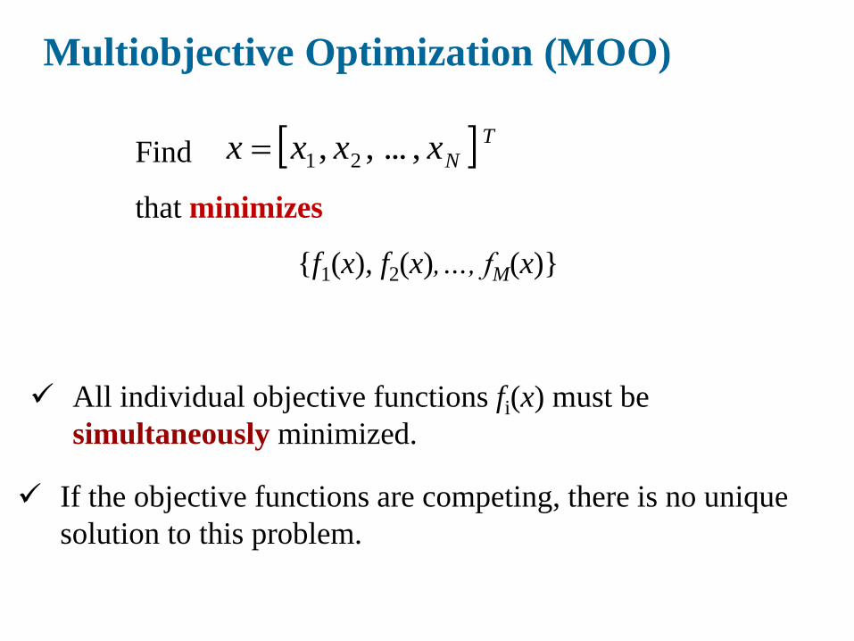
Multiobjective Optimization (MOO)

Find

that minimizes

{f1(x), f2(x),…, fM(x)}

T

Nxxxx ,...,, 21

All individual objective functions fi(x) must be

simultaneously minimized.

If the objective functions are competing, there is no unique

solution to this problem.

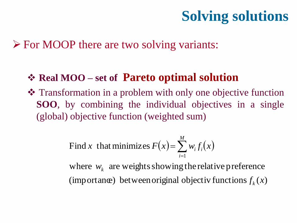
Solving solutions

For MOOP there are two solving variants:

Real MOO – set of Pareto optimal solution

Transformation in a problem with only one objective function

SOO, by combining the individual objectives in a single

(global) objective function (weighted sum)

)( functions objectiv originalbetween e)(importanc

preference relative theshowing weightsare where

minimizes that Find1

xf

w

xfwxFx

k

k

M

i

ii

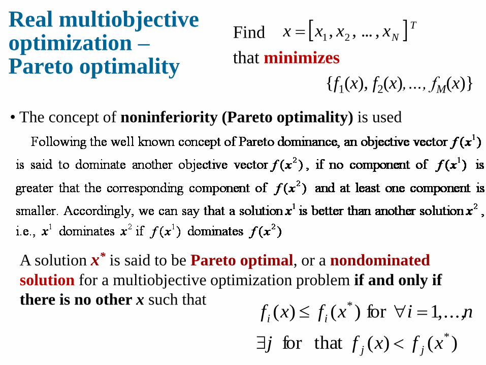
Real multiobjective optimization –Pareto optimality

• The concept of noninferiority (Pareto optimality) is used

A solution x* is said to be Pareto optimal, or a nondominated

solution for a multiobjective optimization problem if and only if

there is no other x such that

)()(thatfor

,...,1for)()(

*

*

xfxfj

nixfxf

jj

ii

Find

that minimizes

{f1(x), f2(x),…, fM(x)}

T

Nxxxx ,...,, 21

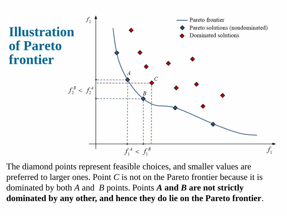
Illustration of Pareto frontier

The diamond points represent feasible choices, and smaller values are

preferred to larger ones. Point C is not on the Pareto frontier because it is

dominated by both A and B points. Points A and B are not strictly

dominated by any other, and hence they do lie on the Pareto frontier.

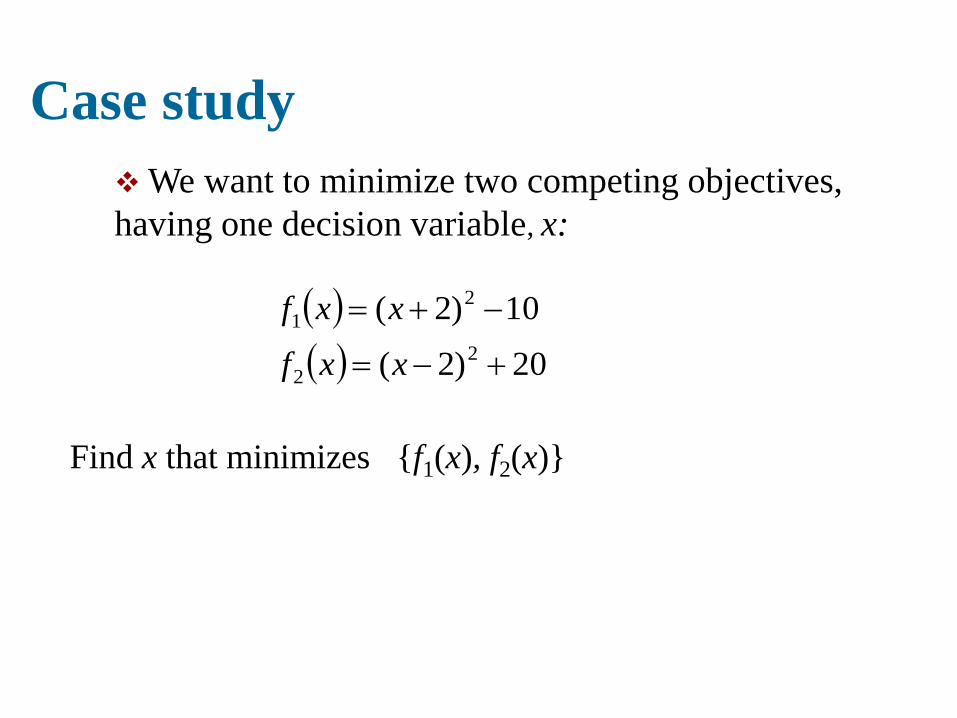
Case study

We want to minimize two competing objectives,

having one decision variable, x:

20)2(

10)2(

2

2

2

1

xxf

xxf

Find x that minimizes {f1(x), f2(x)}

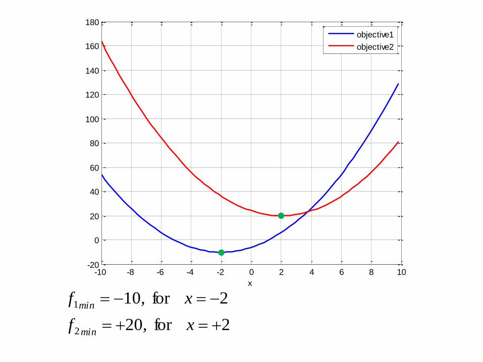
2for20

2for10

2

1

x,f

x,f

min

min

-10 -8 -6 -4 -2 0 2 4 6 8 10-20

0

20

40

60

80

100

120

140

160

180

x

objective1

objective2

Methods to solve

Transformation to a SOO, (using a weighted sum)

and optimize one objective

One single solution: one individual

Use a real MOO (multiobjective ranking )

Multiple solutions: Pareto frontier

Fitness assignment: multiobjective ranking

Each individual in a population receives a rank according to its

quality.

All solutions found during optimization and nondominated by a

different solution constitute the Pareto optimal solutions set – rank 1.

Rank 1 individuals are the best;

Rank 2 individuals are dominated only by rank 1 individuals

Rank 3 individuals are dominated only by rank 1 and rank 2

individuals

…..

MOO using GA

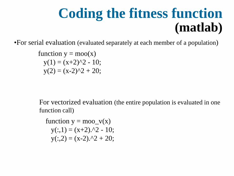
Coding the fitness function (matlab)

function y = moo(x)

y(1) = (x+2)^2 - 10;

y(2) = (x-2)^2 + 20;

•For serial evaluation (evaluated separately at each member of a population)

function y = moo_v(x)

y(:,1) = (x+2).^2 - 10;

y(:,2) = (x-2).^2 + 20;

For vectorized evaluation (the entire population is evaluated in one

function call)

Minimizing Using GAMULTIOBJ

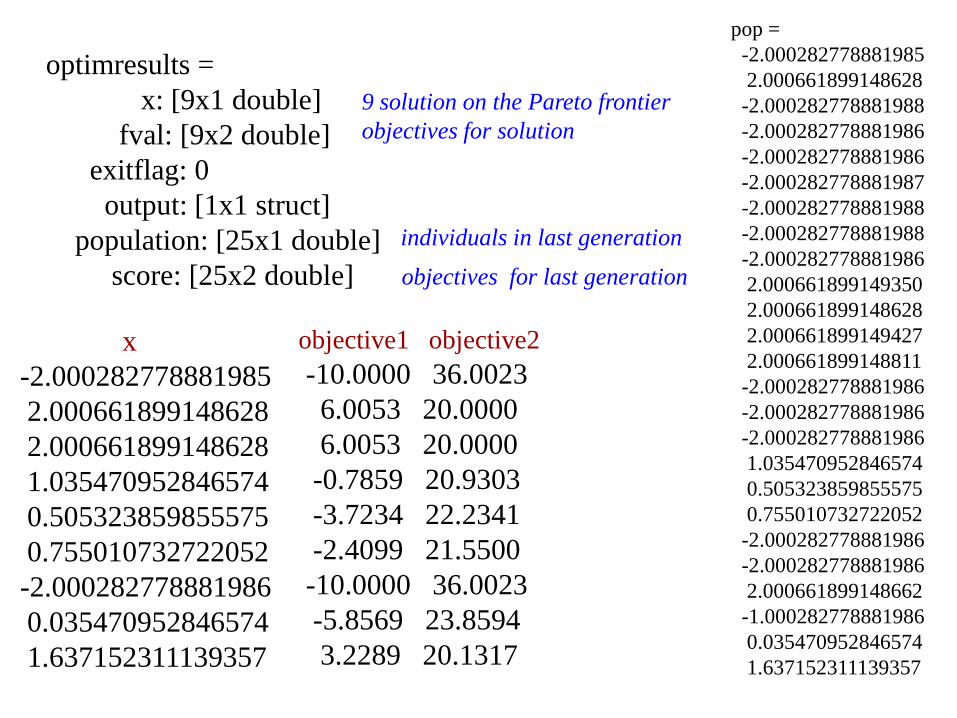
optimresults =

x: [9x1 double]

fval: [9x2 double]

exitflag: 0

output: [1x1 struct]

population: [25x1 double]

score: [25x2 double]

objective1 objective2

-10.0000 36.0023

6.0053 20.0000

6.0053 20.0000

-0.7859 20.9303

-3.7234 22.2341

-2.4099 21.5500

-10.0000 36.0023

-5.8569 23.8594

3.2289 20.1317

x

-2.000282778881985

2.000661899148628

2.000661899148628

1.035470952846574

0.505323859855575

0.755010732722052

-2.000282778881986

0.035470952846574

1.637152311139357

pop =

-2.000282778881985

2.000661899148628

-2.000282778881988

-2.000282778881986

-2.000282778881986

-2.000282778881987

-2.000282778881988

-2.000282778881988

-2.000282778881986

2.000661899149350

2.000661899148628

2.000661899149427

2.000661899148811

-2.000282778881986

-2.000282778881986

-2.000282778881986

1.035470952846574

0.505323859855575

0.755010732722052

-2.000282778881986

-2.000282778881986

2.000661899148662

-1.000282778881986

0.035470952846574

1.637152311139357

9 solution on the Pareto frontier

objectives for solution

individuals in last generation

objectives for last generation

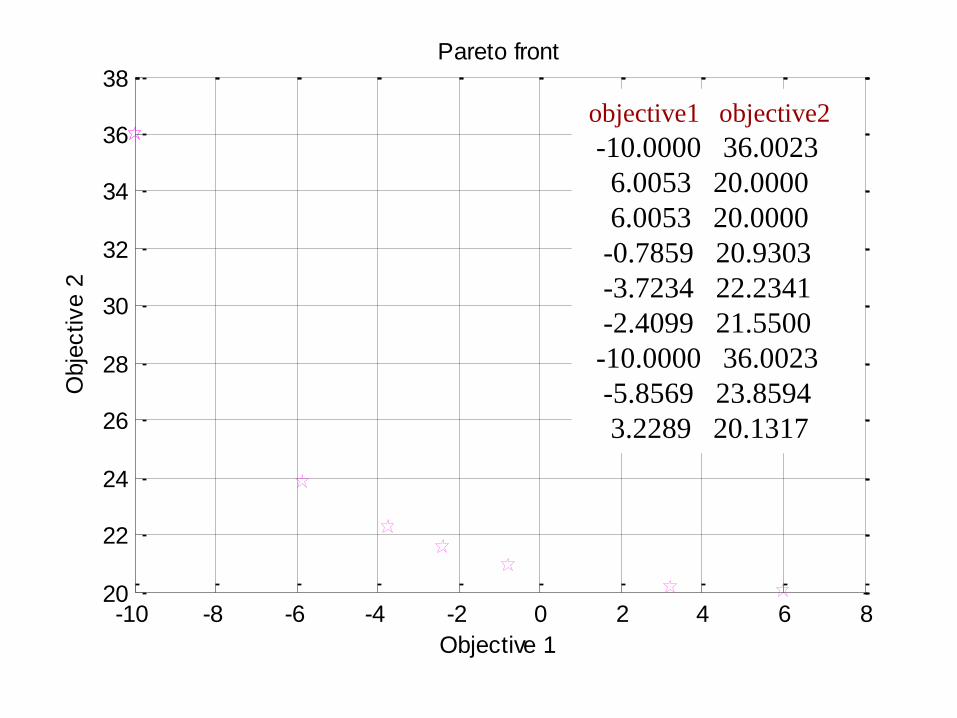
-10 -8 -6 -4 -2 0 2 4 6 820

22

24

26

28

30

32

34

36

38

Objective 1

Obje

ctive 2

Pareto front

objective1 objective2

-10.0000 36.0023

6.0053 20.0000

6.0053 20.0000

-0.7859 20.9303

-3.7234 22.2341

-2.4099 21.5500

-10.0000 36.0023

-5.8569 23.8594

3.2289 20.1317

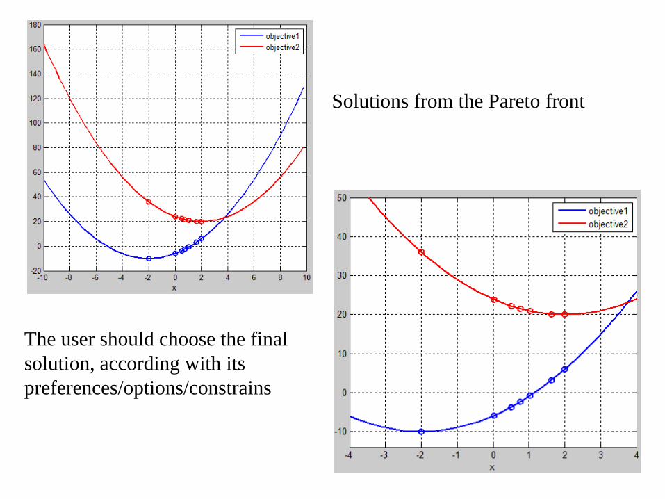
Solutions from the Pareto front

The user should choose the final

solution, according with its

preferences/options/constrains

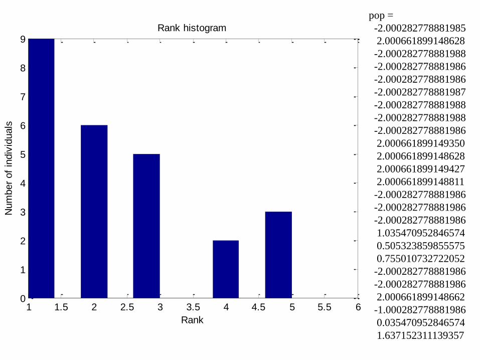
1 1.5 2 2.5 3 3.5 4 4.5 5 5.5 60

1

2

3

4

5

6

7

8

9Rank histogram

Rank

Num

ber

of

indiv

iduals

pop =

-2.000282778881985

2.000661899148628

-2.000282778881988

-2.000282778881986

-2.000282778881986

-2.000282778881987

-2.000282778881988

-2.000282778881988

-2.000282778881986

2.000661899149350

2.000661899148628

2.000661899149427

2.000661899148811

-2.000282778881986

-2.000282778881986

-2.000282778881986

1.035470952846574

0.505323859855575

0.755010732722052

-2.000282778881986

-2.000282778881986

2.000661899148662

-1.000282778881986

0.035470952846574

1.637152311139357

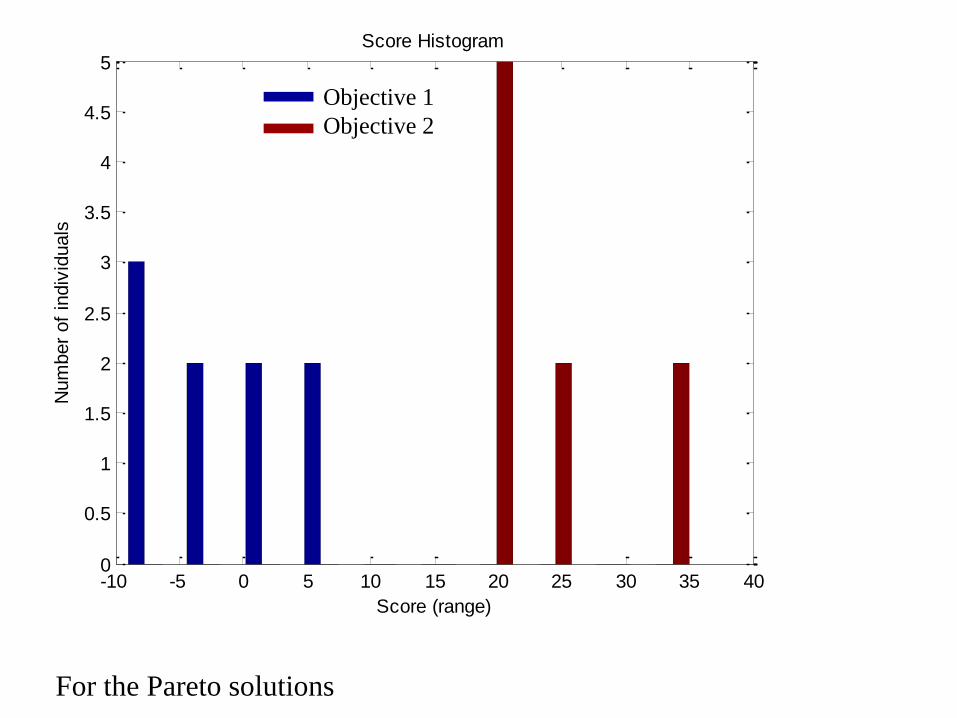
For the Pareto solutions

-10 -5 0 5 10 15 20 25 30 35 400

0.5

1

1.5

2

2.5

3

3.5

4

4.5

5Score Histogram

Score (range)

Num

ber

of

indiv

iduals

Objective 1

Objective 2

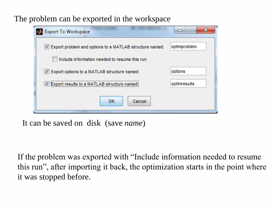
The problem can be exported in the workspace

If the problem was exported with “Include information needed to resume

this run”, after importing it back, the optimization starts in the point where

it was stopped before.

It can be saved on disk (save name)

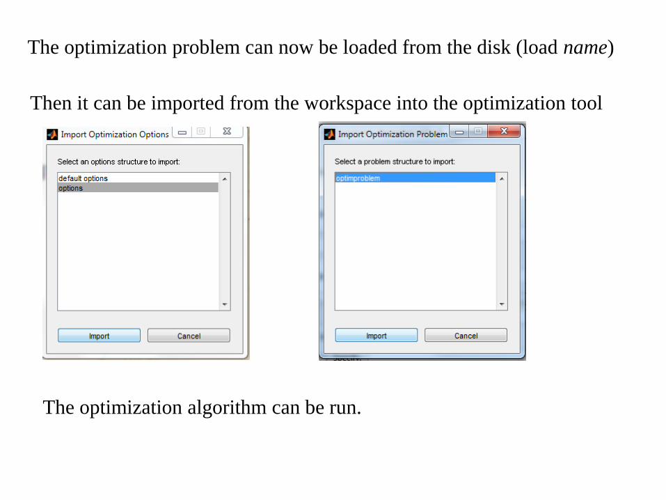
Then it can be imported from the workspace into the optimization tool

The optimization algorithm can be run.

The optimization problem can now be loaded from the disk (load name)

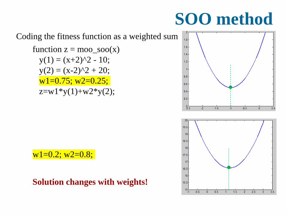
SOO methodCoding the fitness function as a weighted sum

function z = moo_soo(x)

y(1) = (x+2)^2 - 10;

y(2) = (x-2)^2 + 20;

w1=0.75; w2=0.25;

z=w1*y(1)+w2*y(2);

w1=0.2; w2=0.8;

Solution changes with weights!

Computational Intelligence in Complex Decision Systems G. Oltean

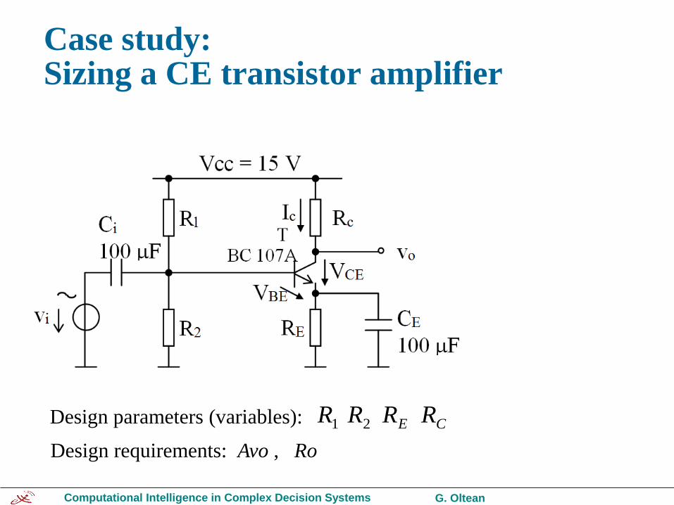
Design parameters (variables): CE RRRR 21

Design requirements: Avo , Ro

Case study: Sizing a CE transistor amplifier


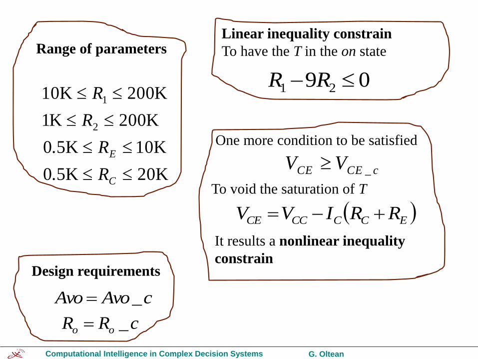
Range of parameters

K20K50

K10K50

K200K1

K200K10

2

1

C

E

R.

R.

R

R09 21 RR

One more condition to be satisfied

c_CECE VV

To void the saturation of T

Design requirements

c_AvoAvo

c_RR oo

ECCCCCE RRIVV

It results a nonlinear inequality

constrain

Linear inequality constrain

To have the T in the on state


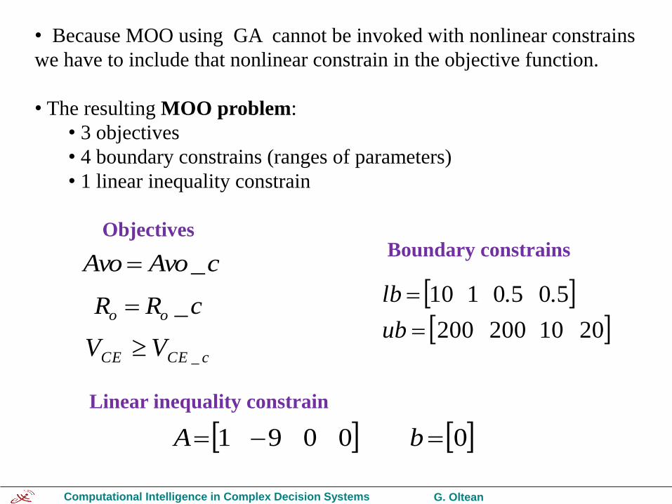
• Because MOO using GA cannot be invoked with nonlinear constrains

we have to include that nonlinear constrain in the objective function.

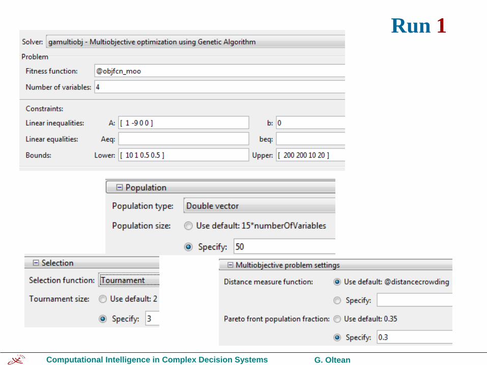
• The resulting MOO problem:

• 3 objectives

• 4 boundary constrains (ranges of parameters)

• 1 linear inequality constrain

c_CECE VV

c_AvoAvo

c_RR oo

ObjectivesBoundary constrains

2010200200

5050110

ub

..lb

Linear inequality constrain

00091 bA


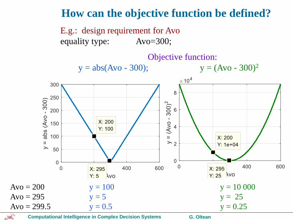
How can the objective function be defined?

E.g.: design requirement for Avo

equality type: Avo = 300;

Objective function:

y = ?


How can the objective function be defined?

E.g.: design requirement for Avo

equality type: Avo=300;

Objective function:

y = abs(Avo - 300); y = (Avo - 300)2

Avo = 200 y = 100 y = 10 000

Avo = 295 y = 5 y = 25

Avo = 299.5 y = 0.5 y = 0.25


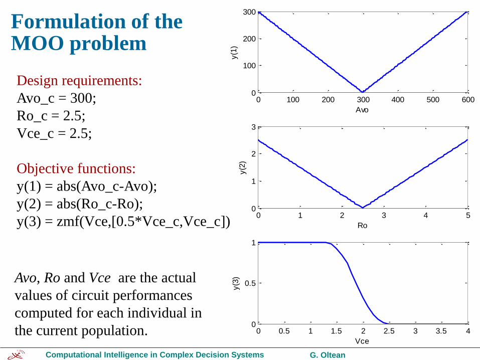
Formulation of the MOO problem

Design requirements:

Avo_c = 300;

Ro_c = 2.5;

Vce_c = 2.5;

Objective functions:

y(1) = abs(Avo_c-Avo);

y(2) = abs(Ro_c-Ro);

y(3) = zmf(Vce,[0.5*Vce_c,Vce_c])

0 100 200 300 400 500 6000

100

200

300

Avo

y(1

)

0 1 2 3 4 50

1

2

3

Ro

y(2

)

0 0.5 1 1.5 2 2.5 3 3.5 40

0.5

1

Vce

y(3

)Avo, Ro and Vce are the actual

values of circuit performances

computed for each individual in

the current population.


Run 1


1 2 3 4 5 6 7 80

5

10

15Rank histogram

Rank

Num

ber

of

indiv

iduals

20 40 60 80 100 120 140 160 180 20020

30

40

50

60

70

80

90

100

Generation

Averg

ae D

ista

nce

Average Distance Between Individuals

0 20 40 60 80 100 120 140 160 180 2000

0.1

0.2

0.3

0.4

0.5

0.6

0.7

0.8

0.9

1

Generation

Avera

ge S

pre

ad

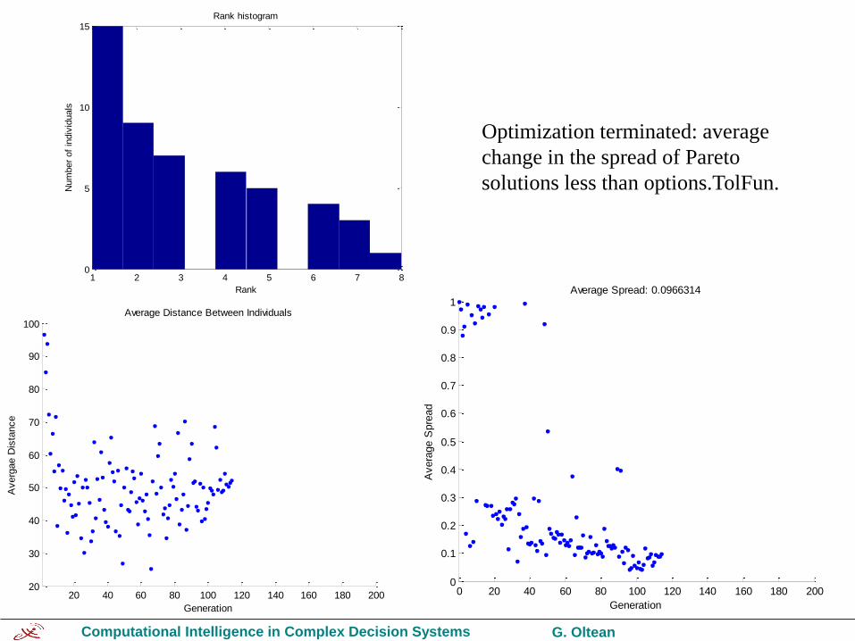
Average Spread: 0.0966314

Optimization terminated: average

change in the spread of Pareto

solutions less than options.TolFun.


0 20 40 60 80 100 1200

1

2

3

4

5

6

7

8

9

10

Objective 1

Obje

ctive 2

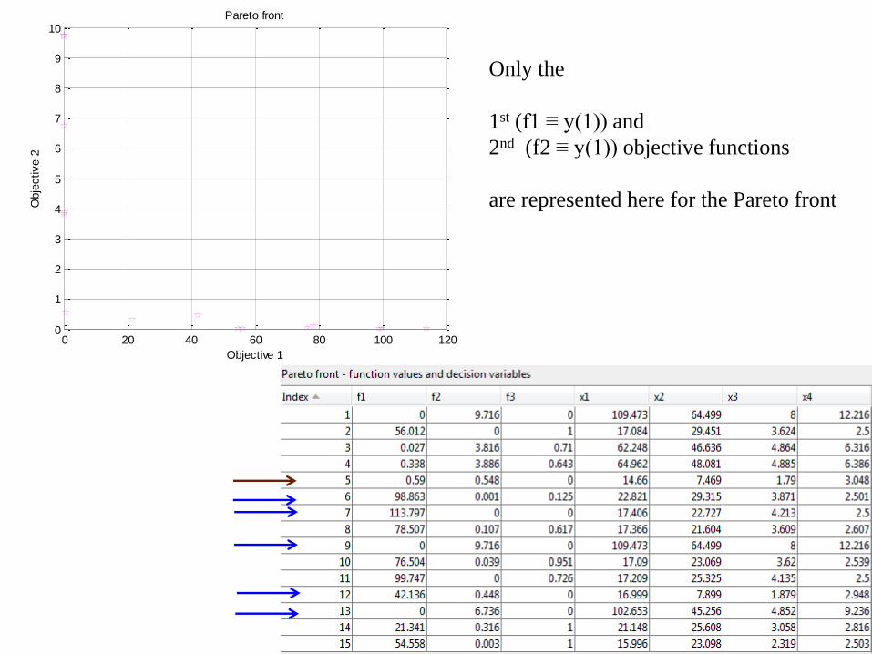
Pareto front

Only the

1st (f1 ≡ y(1)) and

2nd (f2 ≡ y(1)) objective functions

are represented here for the Pareto front


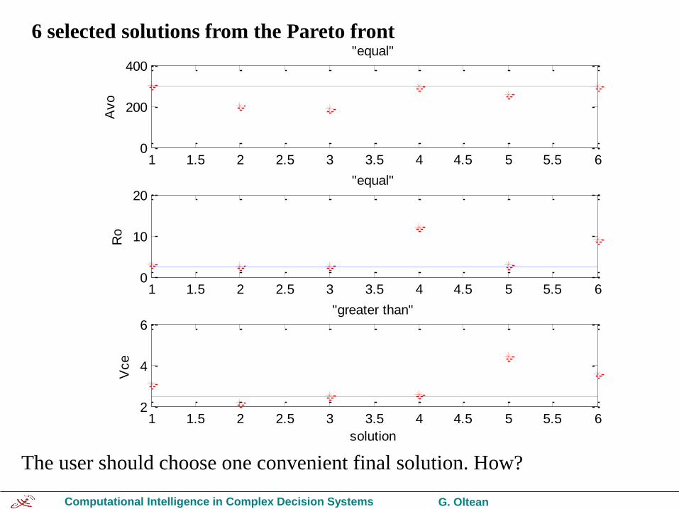
1 1.5 2 2.5 3 3.5 4 4.5 5 5.5 60

200

400

Avo

"equal"

1 1.5 2 2.5 3 3.5 4 4.5 5 5.5 60

10

20

Ro

"equal"

1 1.5 2 2.5 3 3.5 4 4.5 5 5.5 62

4

6

Vce

solution

"greater than"

6 selected solutions from the Pareto front

The user should choose one convenient final solution. How?


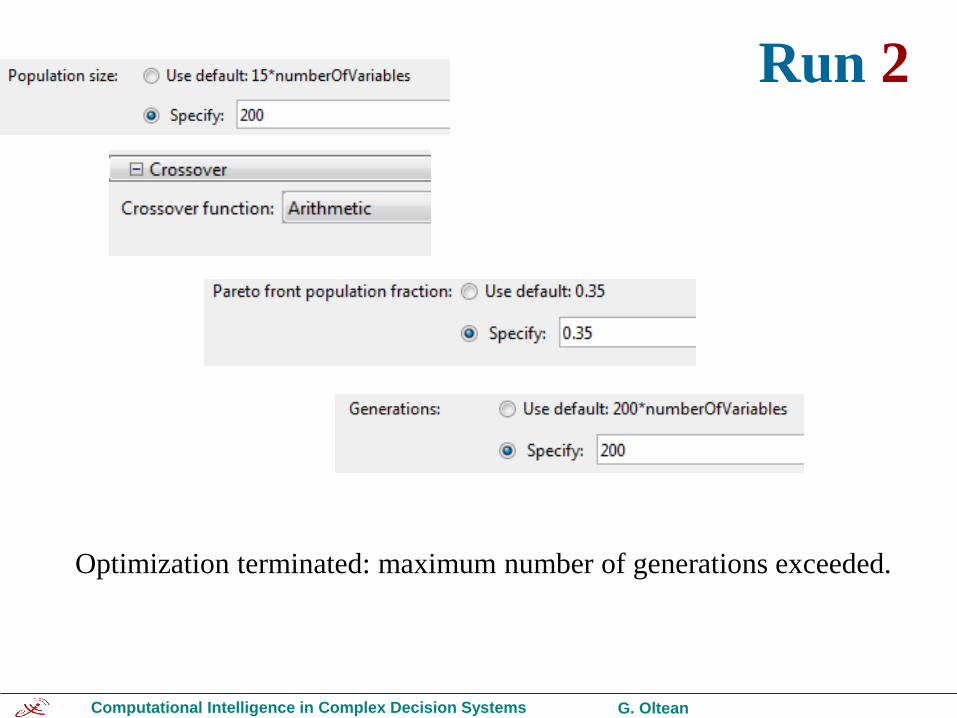
Run 2

Optimization terminated: maximum number of generations exceeded.


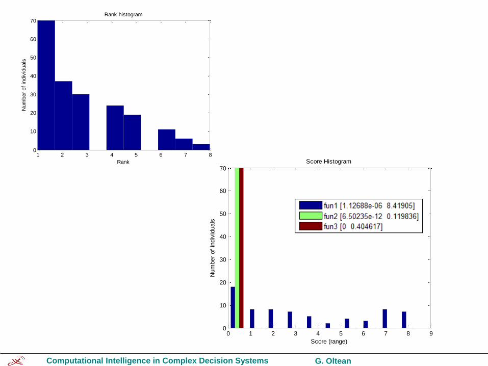
1 2 3 4 5 6 7 80

10

20

30

40

50

60

70Rank histogram

Rank

Num

ber

of

indiv

iduals

0 1 2 3 4 5 6 7 8 90

10

20

30

40

50

60

70Score Histogram

Score (range)

Num

ber

of

indiv

iduals


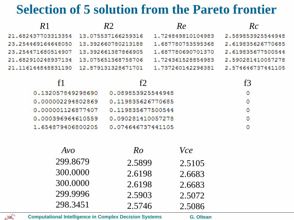
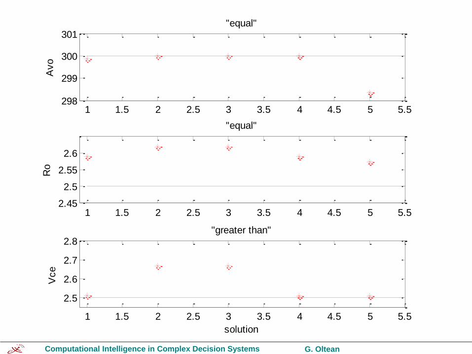
Selection of 5 solution from the Pareto frontier

R1 R2 Re Rc

Avo Ro Vce

f1 f2 f3

299.8679

300.0000

300.0000

299.9996

298.3451

2.5899

2.6198

2.6198

2.5903

2.5746

2.5105

2.6683

2.6683

2.5072

2.5086


1 1.5 2 2.5 3 3.5 4 4.5 5 5.5298

299

300

301

Avo

"equal"

1 1.5 2 2.5 3 3.5 4 4.5 5 5.52.45

2.5

2.55

2.6

Ro

"equal"

1 1.5 2 2.5 3 3.5 4 4.5 5 5.5

2.5

2.6

2.7

2.8

Vce

solution

"greater than"


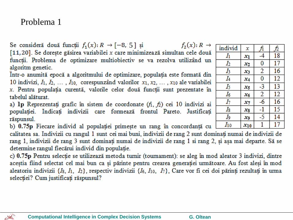
Problema 1

5


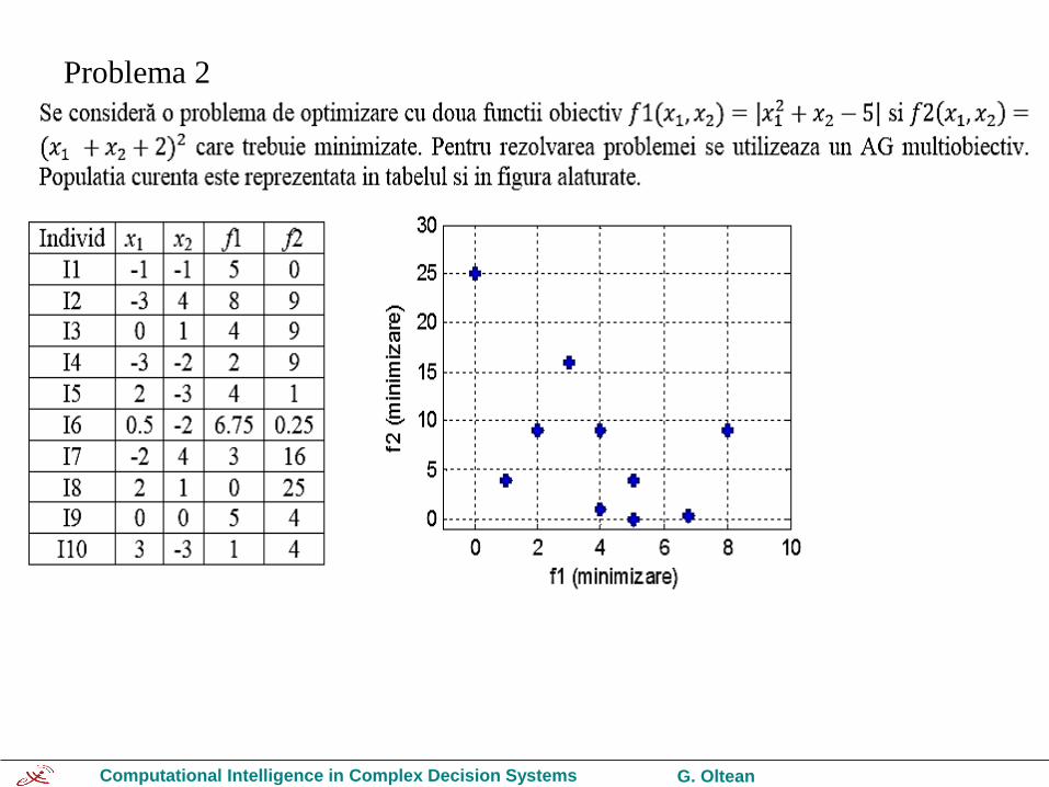
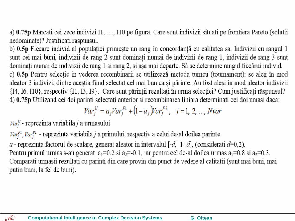
Problema 2


Documents

Optimizare multiobiectiv utilizand algoritmi genetici ... · Optimizare multiobiectiv utilizand algoritmi genetici Multiobjective optimization using genetic algorithms