Optimally-Discriminative Voxel-Based Morphometry ... · Optimally-Discriminative Voxel-Based Morphometry signiﬁcantly increases the ability to detect group differences in schizophrenia,

NeuroImage 79 (2013) 94–110

Contents lists available at SciVerse ScienceDirect

NeuroImage

j ourna l homepage: www.e lsev ie r .com/ locate /yn img

Optimally-Discriminative Voxel-Based Morphometry significantly increases theability to detect group differences in schizophrenia, mild cognitive impairment, andAlzheimer's disease

Tianhao Zhang ⁎, Christos DavatzikosSection of Biomedical Image Analysis, Department of Radiology, University of Pennsylvania, PA, USA

⁎ Corresponding author. Fax: +1 2156140266.E-mail addresses: [email protected], z

1053-8119/$ – see front matter © 2013 Elsevier Inc. Allhttp://dx.doi.org/10.1016/j.neuroimage.2013.04.063

a b s t r a c t
a r t i c l e i n f o
Article history:Accepted 18 April 2013Available online 28 April 2013

Keywords:Voxel-Based MorphometryGeneral Linear ModelSchizophreniaMild cognitive impairmentAlzheimer's diseaseODVBA

Optimally-Discriminative Voxel-Based Analysis (ODVBA) (Zhang and Davatzikos, 2011) is a recently-developed and validated framework of voxel-based group analysis, which transcends limitations of tradition-al Gaussian smoothing in the forms of analysis such as the General Linear Model (GLM). ODVBA estimates theoptimal non-stationary and anisotropic filtering of the data prior to statistical analyses to maximize theability to detect group differences. In this paper, we extensively evaluate ODVBA to three sets of previouslypublished data from studies in schizophrenia, mild cognitive impairment, and Alzheimer's disease, and eval-uate the regions of structural difference identified by ODVBA versus standard Gaussian smoothing and otherrelated methods. The experimental results suggest that ODVBA is considerably more sensitive in detectinggroup differences, presumably because of its ability to adapt the regional filtering to the underlying extentand shape of a group difference, thereby maximizing the ability to detect such difference. Although there isno gold standard in these clinical studies, ODVBA demonstrated highest significance in group differenceswithin the identified voxels. In terms of spatial extent of detected area, agreement of anatomical boundary,and classification, it performed better than other tested voxel-based methods and competitively with thecluster enhancing methods.

© 2013 Elsevier Inc. All rights reserved.

Introduction

Voxel-Based Morphometry (VBM) (Ashburner and Friston, 2000;Davatzikos et al., 2001a; Good et al., 2001), which analyzes thewhole brain in an automated manner, has been developed to char-acterize brain changes on structural Magnetic Resonance Imaging(MRI), without defining labor-intensive and potentially-biasedregions of interest (ROIs). To date, VBM has been widely applied ininvestigating different types of brain disorders, including schizophre-nia, mild cognitive impairment (MCI), and Alzheimer's disease (AD).However, in conventional VBMmethods which implement the GeneralLinear Model (GLM) (Friston et al., 1994), integrating imaging signalsfrom a region using Gaussian pre-smoothing proves challenging dueto the difficulty in selecting the appropriate kernel size (Jones et al.,2005; Zhang et al., 2008). If the kernel is too small for the task, statisticalpower is lost and large numbers of false negatives are bound to con-found the analysis; if the kernel is too large, the extensive smoothingwill reduce both sensitivity and spatial resolution, typically blurring

[email protected] (T. Zhang).

rights reserved.

unrelated structural regions and leading to false positive conclusionsabout the origin of the structural abnormalities.

Most importantly, Gaussian smoothing will always lack the spatialadaptivity necessary to optimally match image filtering with anunderlying (unknown a priori) region of interest. Some spatiallyadaptive methods have been developed to address this drawback.Davatzikos et al. (2001b) developed a spatially adaptive filter whoseshape changes with the assistance of a pre-defined atlas (alsoknown as ROIs). This method would be effective if true group abnor-malities coincide with these pre-defined anatomical boundaries, butthis is not always the case. More generally in image processing, fulldata-driven spatially adaptive methods which do not require ROIshave been pursued in various contexts. Perona and Malik (1990)developed the Anisotropic Diffusion scheme which removes noiseusing gradient information while preserving object boundaries. Thismethod was subsequently extended (Gerig et al., 1992) into MRIapplications. Polzehl and Spokoiny (2000, 2006) proposed a localdensity estimation-based method for adaptive weights smoothing,named Propagation–Separation (PS), which preserves spatial extentand shapes of the activated regions in images having large homoge-neous areas and sharp discontinuities. This method has subsequentlybeen applied to fMRI activation detection (Tabelow et al., 2006). Awavelet-based denoising method was proposed by Pizurica et al.

http://dx.doi.org/10.1016/j.neuroimage.2013.04.063

mailto:[email protected]

mailto:[email protected]

http://dx.doi.org/10.1016/j.neuroimage.2013.04.063

http://www.sciencedirect.com/science/journal/10538119

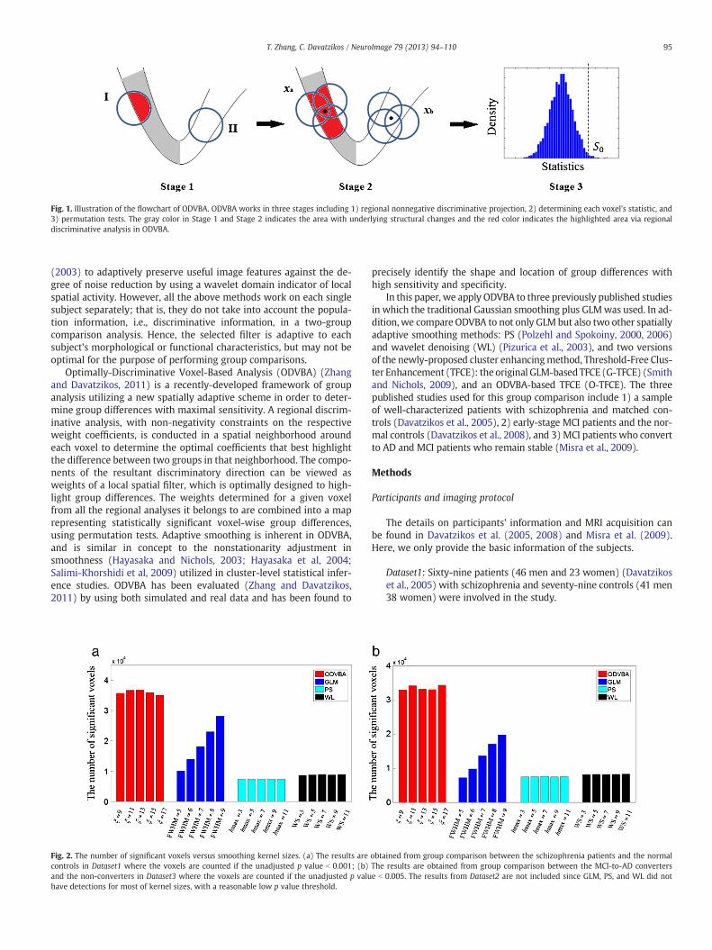
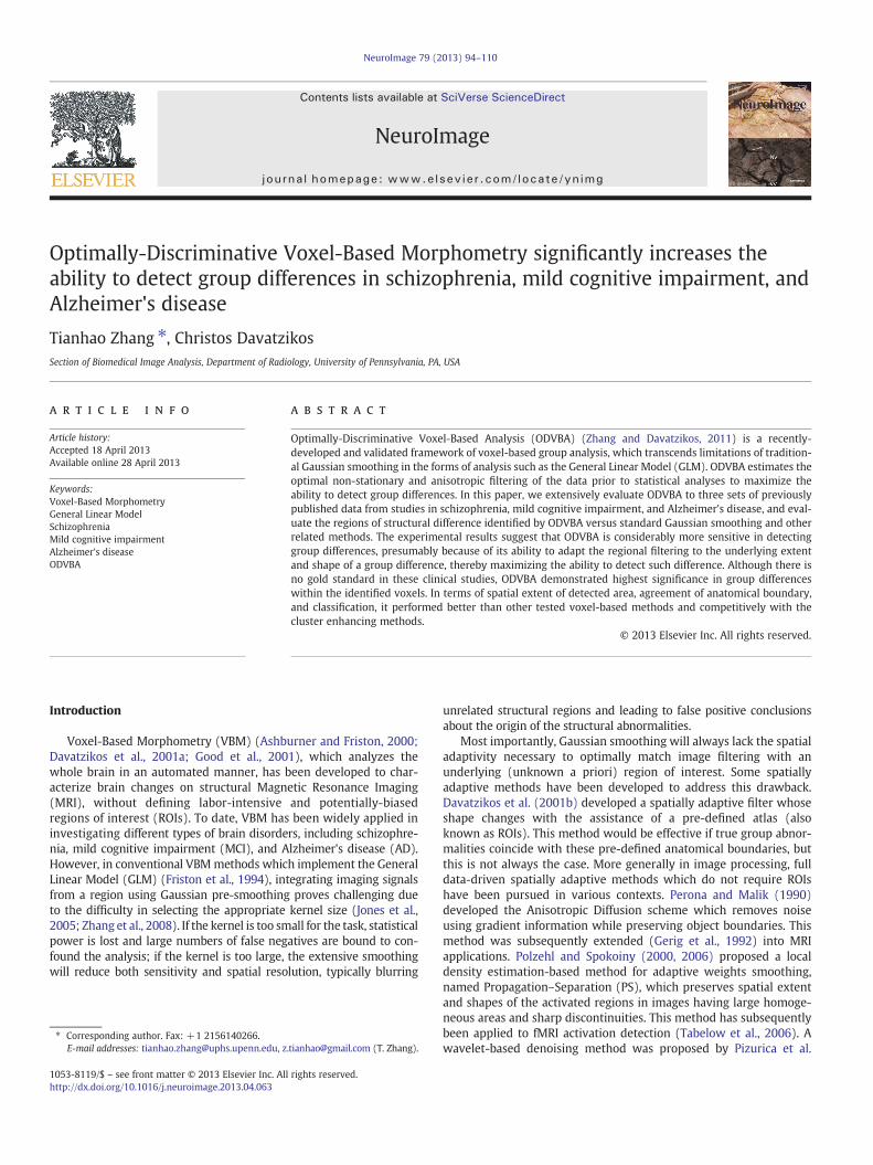
Fig. 1. Illustration of the flowchart of ODVBA. ODVBA works in three stages including 1) regional nonnegative discriminative projection, 2) determining each voxel's statistic, and3) permutation tests. The gray color in Stage 1 and Stage 2 indicates the area with underlying structural changes and the red color indicates the highlighted area via regionaldiscriminative analysis in ODVBA.

95T. Zhang, C. Davatzikos / NeuroImage 79 (2013) 94–110

(2003) to adaptively preserve useful image features against the de-gree of noise reduction by using a wavelet domain indicator of localspatial activity. However, all the above methods work on each singlesubject separately; that is, they do not take into account the popula-tion information, i.e., discriminative information, in a two-groupcomparison analysis. Hence, the selected filter is adaptive to eachsubject's morphological or functional characteristics, but may not beoptimal for the purpose of performing group comparisons.

Optimally-Discriminative Voxel-Based Analysis (ODVBA) (Zhangand Davatzikos, 2011) is a recently-developed framework of groupanalysis utilizing a new spatially adaptive scheme in order to deter-mine group differences with maximal sensitivity. A regional discrim-inative analysis, with non-negativity constraints on the respectiveweight coefficients, is conducted in a spatial neighborhood aroundeach voxel to determine the optimal coefficients that best highlightthe difference between two groups in that neighborhood. The compo-nents of the resultant discriminatory direction can be viewed asweights of a local spatial filter, which is optimally designed to high-light group differences. The weights determined for a given voxelfrom all the regional analyses it belongs to are combined into a maprepresenting statistically significant voxel-wise group differences,using permutation tests. Adaptive smoothing is inherent in ODVBA,and is similar in concept to the nonstationarity adjustment insmoothness (Hayasaka and Nichols, 2003; Hayasaka et al, 2004;Salimi-Khorshidi et al, 2009) utilized in cluster-level statistical infer-ence studies. ODVBA has been evaluated (Zhang and Davatzikos,2011) by using both simulated and real data and has been found to

Fig. 2. The number of significant voxels versus smoothing kernel sizes. (a) The results arecontrols in Dataset1 where the voxels are counted if the unadjusted p value b 0.001; (b)and the non-converters in Dataset3 where the voxels are counted if the unadjusted p valuhave detections for most of kernel sizes, with a reasonable low p value threshold.

precisely identify the shape and location of group differences withhigh sensitivity and specificity.

In this paper, we apply ODVBA to three previously published studiesin which the traditional Gaussian smoothing plus GLMwas used. In ad-dition, we compare ODVBA to not only GLM but also two other spatiallyadaptive smoothing methods: PS (Polzehl and Spokoiny, 2000, 2006)and wavelet denoising (WL) (Pizurica et al., 2003), and two versionsof the newly-proposed cluster enhancingmethod, Threshold-Free Clus-ter Enhancement (TFCE): the original GLM-based TFCE (G-TFCE) (Smithand Nichols, 2009), and an ODVBA-based TFCE (O-TFCE). The threepublished studies used for this group comparison include 1) a sampleof well-characterized patients with schizophrenia and matched con-trols (Davatzikos et al., 2005), 2) early-stage MCI patients and the nor-mal controls (Davatzikos et al., 2008), and 3) MCI patients who convertto AD and MCI patients who remain stable (Misra et al., 2009).

Methods

Participants and imaging protocol

The details on participants' information and MRI acquisition canbe found in Davatzikos et al. (2005, 2008) and Misra et al. (2009).Here, we only provide the basic information of the subjects.

Dataset1: Sixty-nine patients (46 men and 23 women) (Davatzikoset al., 2005) with schizophrenia and seventy-nine controls (41 men38 women) were involved in the study.

obtained from group comparison between the schizophrenia patients and the normalThe results are obtained from group comparison between the MCI-to-AD converterse b 0.005. The results from Dataset2 are not included since GLM, PS, and WL did not

96 T. Zhang, C. Davatzikos / NeuroImage 79 (2013) 94–110

Dataset2: Thirty older adults (Davatzikos et al., 2008) including 15subjects with MCI and 15 normal controls were examined in thecurrent study.Dataset3: One hundred subjects with MCI were randomly selectedfrom the data used in Misra et al. (2009). 50 of these subjects hadundergone conversion to AD. The remaining 50 are non-converters.

Image processing

A standard image pre-processing protocol described in Goldszal et al.(1998) was used in all three parent studies. The result was a RAVENSmap, reflecting regional volumetrics (Davatzikos et al., 2001a; Goldszalet al., 1998; Shen and Davatzikos, 2002), akin to what was typically

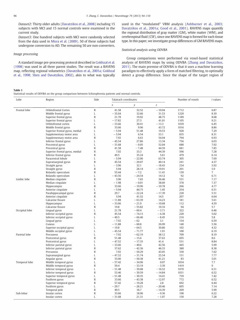
Table 1Statistical results of ODVBA on the group comparison between Schizophrenia patients and

Lobe Region Side Talairac

x

Frontal lobe Orbitofrontal Cortex R 41.58Middle frontal gyrus L −35.64Superior frontal gyrus R 21.78Superior frontal gyrus L −17.82Orbitofrontal cortex L −33.66Middle frontal gyrus R 33.66Superior frontal gyrus, medial L −5.94Supplementary motor area L −5.94Supplementary motor area R 7.92Inferior frontal gyrus L −45.54Precentral gyrus L −31.68Precentral gyrus R 41.58Superior frontal gyrus, medial R 7.92Inferior frontal gyrus R 49.5Paracentral lobule L −5.94Supramarginal gyrus R 45.54Straight gyrus L −3.96Straight gyrus R 5.94Rolandic operculum R 55.44Rolandic operculum L −43.56

Limbic lobe Median cingulate R 3.96Median cingulate L −1.98Hippocampus R 33.66Anterior cingulate L −5.94Parahippocampal gyrus R 29.7Anterior cingulate R 5.94Calcarine fissure L −11.88Hippocampus L −33.66Calcarine fissure R 19.8

Occipital lobe Lingual gyrus L 21.78Inferior occipital gyrus R 45.54Inferior occipital gyrus L −49.5Lingual gyrus L −7.92Cuneus L −11.88Superior occipital gyrus L −19.8Middle occipital gyrus L −45.54

Parietal lobe Precuneus L −7.92Postcentral gyrus R 51.48Postcentral gyrus L −47.52Inferior parietal gyrus L −33.66Inferior parietal gyrus R 37.62Precuneus R 7.92Supramarginal gyrus L −47.52Angular gyrus R 33.66

Temporal lobe Middle temporal gyrus L −57.42Middle temporal gyrus R 59.4Inferior temporal gyrus L −51.48Inferior temporal gyrus R 53.46Superior temporal gyrus L −51.48Fusiform gyrus R 33.66Superior temporal gyrus R 57.42Fusiform gyrus L −29.7Temporal pole R 49.5

Sub-lobar Insular cortex R 33.66Insular cortex L −31.68

used in the “modulated” VBM analysis (Ashburner et al., 2003;Davatzikos et al., 2001a; Good et al., 2001). RAVENS maps quantifythe regional distribution of gray matter (GM), white matter (WM), andcerebrospinalfluid (CSF), since one RAVENSmap is formed for each tissuetype. In this paper, we investigate group differences of GMRAVENSmaps.

Statistical analysis using ODVBA

Group comparisons were performed via voxel-based statisticalanalysis of RAVENS maps by using ODVBA (Zhang and Davatzikos,2011). The main premise of ODVBA is that it uses a machine learningparadigm to effectively apply a form of matched filtering, to optimallydetect a group difference. Since the shape of the target region of

normal controls.

h coordinates Number of voxels t values

y z

32.52 −10.04 1712 6.8732.66 31.53 1220 8.3919.92 48.75 1189 8.6827.3 41.01 1105 9.2130.41 −13.3 1039 6.459.96 43.72 1016 8.86

51.48 19.53 928 7.296.54 53.1 835 8.316.63 54.94 794 6.93

27.86 13.34 756 6.03−9.05 52.04 688 7.92−7.48 44.59 681 7.8533.3 44.39 596 7.2835.24 5.61 479 6.14

−22.06 63.74 305 7.69−29.07 40.14 241 4.37

32.1 −18.43 234 5.9228.14 −19.91 201 5.9−7.2 11.41 139 7

−24.54 14.12 92 6.717.65 36.46 531 7.17

−0.01 38.69 378 7.37−19.96 −10.78 266 4.77

44.75 1.45 254 6.51−22.24 −17.39 228 5.51

41.52 14.5 207 6.64−63.39 14.23 181 5.61−21.9 −10.68 112 4.59−55.82 10.16 94 5.7−60.4 −3.71 322 6.46−74.13 −6.38 220 5.02−66.46 −8.45 216 5.8−62 3.1 154 6.59−60.8 26.99 140 5.56−64.5 30.86 102 4.32−71.77 1.91 100 6.19−62.19 38.12 709 8.19−15.6 37.63 695 8.6−17.35 41.4 531 8.84−40.6 42.56 445 5.99−42.36 46.33 380 8.38−50.29 43.05 330 7.62−31.74 25.54 151 7.77−50.38 41.21 83 5.01−34.96 0.07 1834 7.7−33.19 −3.39 1419 9−39.68 −16.52 1070 6.51−39.59 −14.84 1031 6.52−30.35 14.41 759 7.42−43.38 −12.97 772 6.52−19.28 2.8 692 6.44−28.21 −20.46 605 7.14

18.7 −14.39 269 5.9918.96 −9.36 198 6.2221.31 −1.07 150 7.28

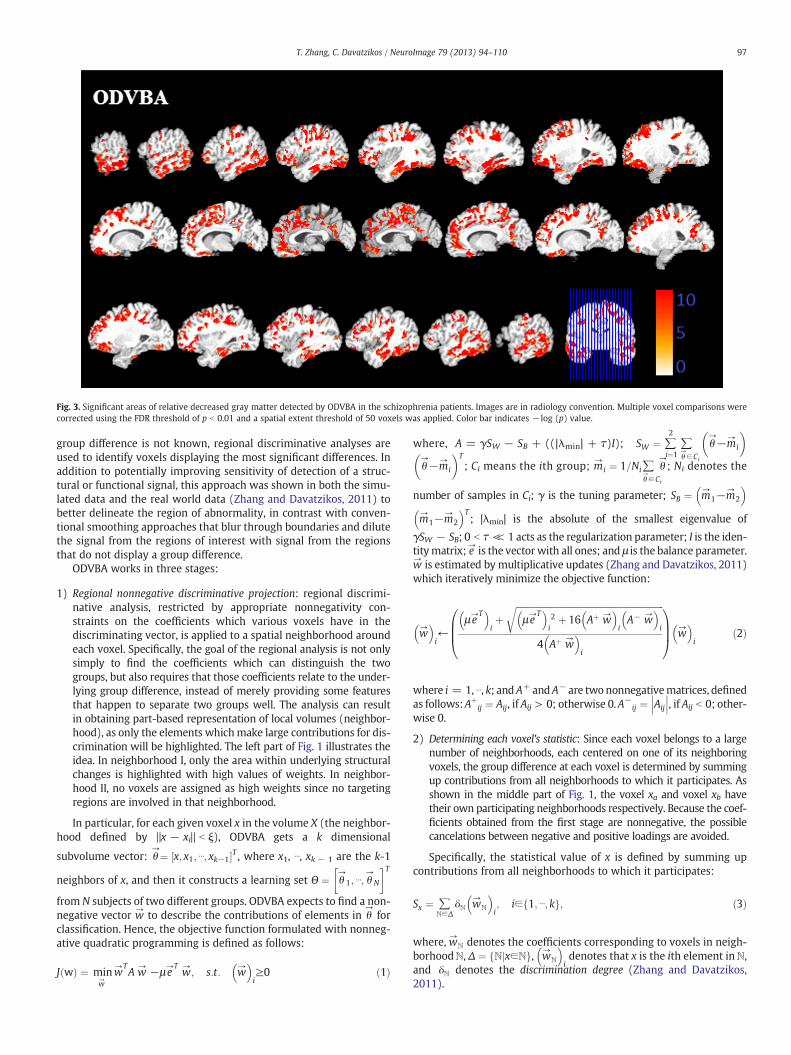
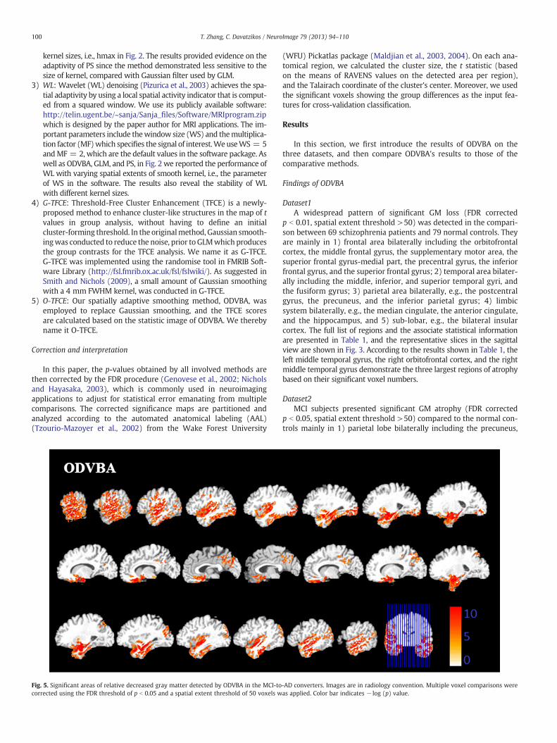
Fig. 3. Significant areas of relative decreased gray matter detected by ODVBA in the schizophrenia patients. Images are in radiology convention. Multiple voxel comparisons werecorrected using the FDR threshold of p b 0.01 and a spatial extent threshold of 50 voxels was applied. Color bar indicates −log (p) value.


group difference is not known, regional discriminative analyses areused to identify voxels displaying the most significant differences. Inaddition to potentially improving sensitivity of detection of a struc-tural or functional signal, this approach was shown in both the simu-lated data and the real world data (Zhang and Davatzikos, 2011) tobetter delineate the region of abnormality, in contrast with conven-tional smoothing approaches that blur through boundaries and dilutethe signal from the regions of interest with signal from the regionsthat do not display a group difference.

ODVBA works in three stages:

1) Regional nonnegative discriminative projection: regional discrimi-native analysis, restricted by appropriate nonnegativity con-straints on the coefficients which various voxels have in thediscriminating vector, is applied to a spatial neighborhood aroundeach voxel. Specifically, the goal of the regional analysis is not onlysimply to find the coefficients which can distinguish the twogroups, but also requires that those coefficients relate to the under-lying group difference, instead of merely providing some featuresthat happen to separate two groups well. The analysis can resultin obtaining part-based representation of local volumes (neighbor-hood), as only the elements whichmake large contributions for dis-crimination will be highlighted. The left part of Fig. 1 illustrates theidea. In neighborhood I, only the area within underlying structuralchanges is highlighted with high values of weights. In neighbor-hood II, no voxels are assigned as high weights since no targetingregions are involved in that neighborhood.

In particular, for each given voxel x in the volume X (the neighbor-hood defined by ‖x − xi‖ b ξ), ODVBA gets a k dimensional

subvolume vector: θ→¼ x; x1; ⋯; xk−1½ �T , where x1, ⋯, xk − 1 are the k-1

neighbors of x, and then it constructs a learning set Θ ¼ θ→

1; ⋯; θ→

N

� �T

from N subjects of two different groups. ODVBA expects to find a non-negative vector w

→to describe the contributions of elements in θ

→for

classification. Hence, the objective function formulated with nonneg-ative quadratic programming is defined as follows:

J wð Þ ¼ minw→

w→T

A w→ −μ e

→Tw→; s:t: w

→� �

i≥0 ð1Þ

where, A = γSW − SB + ((|λmin| + τ)I); SW ¼ ∑i¼1

2

∑θ→∈Ci

θ→−m

→i

� �

θ→−m

→i

� �T

; Ci means the ith group; m→

i ¼ 1=Ni∑θ→∈Ci

θ→; Ni denotes the

number of samples in Ci; γ is the tuning parameter; SB ¼ m→

1−m→

2

� �

m→

1−m→

2

� �T; |λmin| is the absolute of the smallest eigenvalue of

γSW − SB; 0 b τ ≪ 1 acts as the regularization parameter; I is the iden-titymatrix; e

→is the vector with all ones; and μ is the balance parameter.

w→

is estimated by multiplicative updates (Zhang and Davatzikos, 2011)which iteratively minimize the objective function:

w→

� �i←

μ e→T� �

iþ

ffiffiffiffiffiffiffiffiffiffiffiffiffiffiffiffiffiffiffiffiffiffiffiffiffiffiffiffiffiffiffiffiffiffiffiffiffiffiffiffiffiffiffiffiffiffiffiffiffiffiffiffiffiffiffiffiffiffiffiffiffiffiffiffiffiffiffiμ e→T� �

i

2 þ 16 Aþ w→

� �iA− w

→� �

i

r

4 Aþ w→

� �i

0BB@

1CCA w

→� �

ið2Þ

where i = 1, ⋯, k; and A+andA− are twononnegativematrices, definedas follows:Aþ

ij ¼ Aij, if Aij > 0; otherwise 0.A−ij ¼ Aij

, if Aij b 0; other-wise 0.

2) Determining each voxel's statistic: Since each voxel belongs to a largenumber of neighborhoods, each centered on one of its neighboringvoxels, the group difference at each voxel is determined by summingup contributions from all neighborhoods to which it participates. Asshown in the middle part of Fig. 1, the voxel xa and voxel xb havetheir own participating neighborhoods respectively. Because the coef-ficients obtained from the first stage are nonnegative, the possiblecancelations between negative and positive loadings are avoided.

Specifically, the statistical value of x is defined by summing upcontributions from all neighborhoods to which it participates:

Sx ¼ ∑N∈Δ

δN w→

N

� �i; i∈ 1; ⋯; kf g; ð3Þ

where, w→

N denotes the coefficients corresponding to voxels in neigh-borhoodN,Δ ¼ N x∈Nj gf , w

→N

� �idenotes that x is the ith element inN,

and δN denotes the discrimination degree (Zhang and Davatzikos,2011).

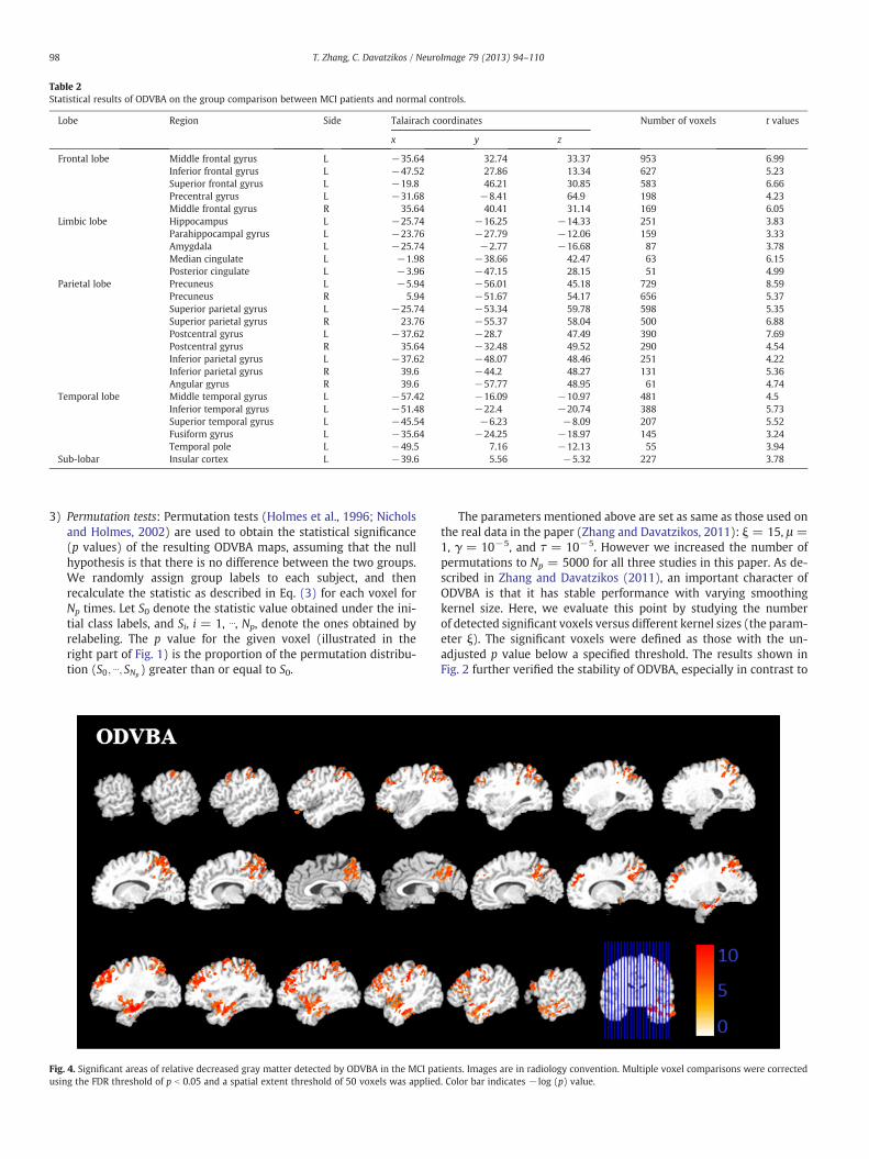
Table 2Statistical results of ODVBA on the group comparison between MCI patients and normal controls.

Lobe Region Side Talairach coordinates Number of voxels t values

x y z

Frontal lobe Middle frontal gyrus L −35.64 32.74 33.37 953 6.99Inferior frontal gyrus L −47.52 27.86 13.34 627 5.23Superior frontal gyrus L −19.8 46.21 30.85 583 6.66Precentral gyrus L −31.68 −8.41 64.9 198 4.23Middle frontal gyrus R 35.64 40.41 31.14 169 6.05

Limbic lobe Hippocampus L −25.74 −16.25 −14.33 251 3.83Parahippocampal gyrus L −23.76 −27.79 −12.06 159 3.33Amygdala L −25.74 −2.77 −16.68 87 3.78Median cingulate L −1.98 −38.66 42.47 63 6.15Posterior cingulate L −3.96 −47.15 28.15 51 4.99

Parietal lobe Precuneus L −5.94 −56.01 45.18 729 8.59Precuneus R 5.94 −51.67 54.17 656 5.37Superior parietal gyrus L −25.74 −53.34 59.78 598 5.35Superior parietal gyrus R 23.76 −55.37 58.04 500 6.88Postcentral gyrus L −37.62 −28.7 47.49 390 7.69Postcentral gyrus R 35.64 −32.48 49.52 290 4.54Inferior parietal gyrus L −37.62 −48.07 48.46 251 4.22Inferior parietal gyrus R 39.6 −44.2 48.27 131 5.36Angular gyrus R 39.6 −57.77 48.95 61 4.74

Temporal lobe Middle temporal gyrus L −57.42 −16.09 −10.97 481 4.5Inferior temporal gyrus L −51.48 −22.4 −20.74 388 5.73Superior temporal gyrus L −45.54 −6.23 −8.09 207 5.52Fusiform gyrus L −35.64 −24.25 −18.97 145 3.24Temporal pole L −49.5 7.16 −12.13 55 3.94

Sub-lobar Insular cortex L −39.6 5.56 −5.32 227 3.78


3) Permutation tests: Permutation tests (Holmes et al., 1996; Nicholsand Holmes, 2002) are used to obtain the statistical significance(p values) of the resulting ODVBA maps, assuming that the nullhypothesis is that there is no difference between the two groups.We randomly assign group labels to each subject, and thenrecalculate the statistic as described in Eq. (3) for each voxel forNp times. Let S0 denote the statistic value obtained under the ini-tial class labels, and Si, i = 1, ⋯, Np, denote the ones obtained byrelabeling. The p value for the given voxel (illustrated in theright part of Fig. 1) is the proportion of the permutation distribu-tion (S0; ⋯; SNp) greater than or equal to S0.

Fig. 4. Significant areas of relative decreased gray matter detected by ODVBA in the MCI pausing the FDR threshold of p b 0.05 and a spatial extent threshold of 50 voxels was applied

The parameters mentioned above are set as same as those used onthe real data in the paper (Zhang and Davatzikos, 2011): ξ = 15, μ =1, γ = 10−5, and τ = 10−5. However we increased the number ofpermutations to Np = 5000 for all three studies in this paper. As de-scribed in Zhang and Davatzikos (2011), an important character ofODVBA is that it has stable performance with varying smoothingkernel size. Here, we evaluate this point by studying the numberof detected significant voxels versus different kernel sizes (the param-eter ξ). The significant voxels were defined as those with the un-adjusted p value below a specified threshold. The results shown inFig. 2 further verified the stability of ODVBA, especially in contrast to

tients. Images are in radiology convention. Multiple voxel comparisons were corrected. Color bar indicates −log (p) value.

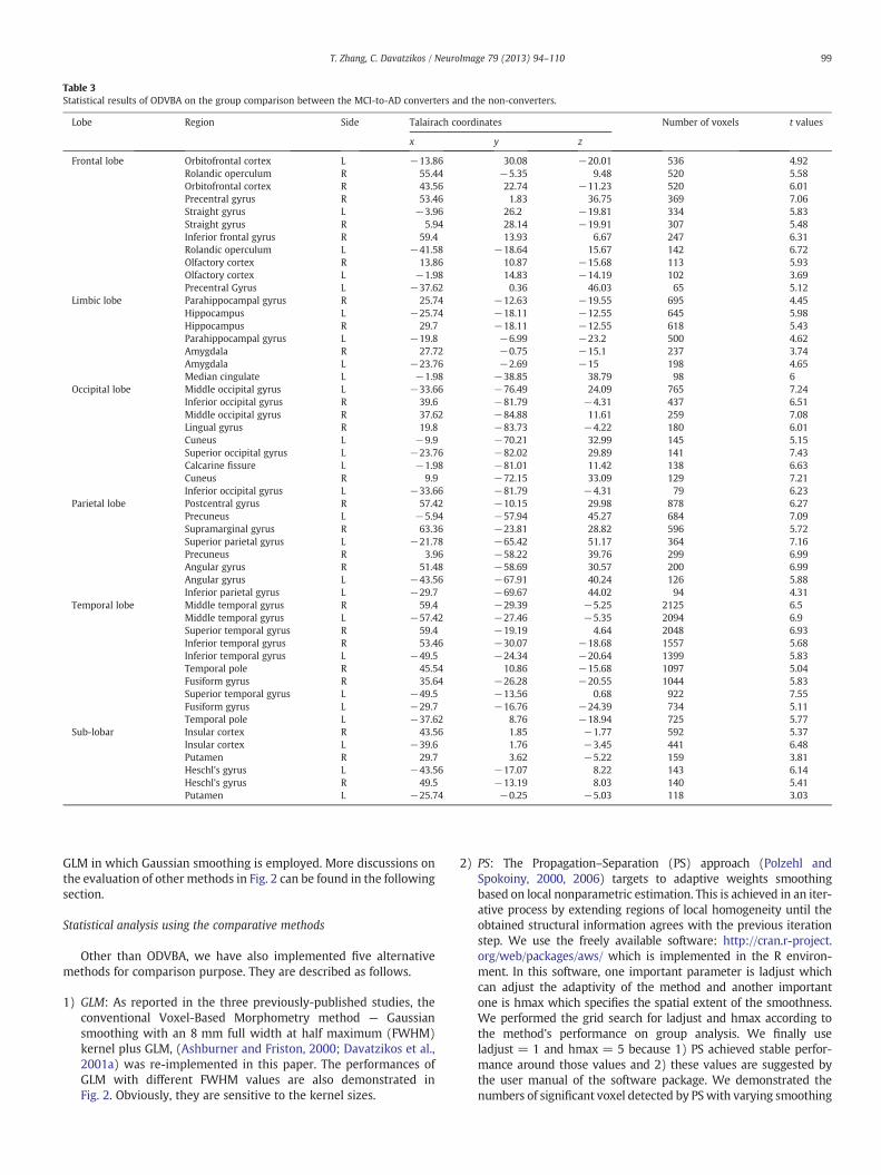
Table 3Statistical results of ODVBA on the group comparison between the MCI-to-AD converters and the non-converters.

Lobe Region Side Talairach coordinates Number of voxels t values

x y z

Frontal lobe Orbitofrontal cortex L −13.86 30.08 −20.01 536 4.92Rolandic operculum R 55.44 −5.35 9.48 520 5.58Orbitofrontal cortex R 43.56 22.74 −11.23 520 6.01Precentral gyrus R 53.46 1.83 36.75 369 7.06Straight gyrus L −3.96 26.2 −19.81 334 5.83Straight gyrus R 5.94 28.14 −19.91 307 5.48Inferior frontal gyrus R 59.4 13.93 6.67 247 6.31Rolandic operculum L −41.58 −18.64 15.67 142 6.72Olfactory cortex R 13.86 10.87 −15.68 113 5.93Olfactory cortex L −1.98 14.83 −14.19 102 3.69Precentral Gyrus L −37.62 0.36 46.03 65 5.12

Limbic lobe Parahippocampal gyrus R 25.74 −12.63 −19.55 695 4.45Hippocampus L −25.74 −18.11 −12.55 645 5.98Hippocampus R 29.7 −18.11 −12.55 618 5.43Parahippocampal gyrus L −19.8 −6.99 −23.2 500 4.62Amygdala R 27.72 −0.75 −15.1 237 3.74Amygdala L −23.76 −2.69 −15 198 4.65Median cingulate L −1.98 −38.85 38.79 98 6

Occipital lobe Middle occipital gyrus L −33.66 −76.49 24.09 765 7.24Inferior occipital gyrus R 39.6 −81.79 −4.31 437 6.51Middle occipital gyrus R 37.62 −84.88 11.61 259 7.08Lingual gyrus R 19.8 −83.73 −4.22 180 6.01Cuneus L −9.9 −70.21 32.99 145 5.15Superior occipital gyrus L −23.76 −82.02 29.89 141 7.43Calcarine fissure L −1.98 −81.01 11.42 138 6.63Cuneus R 9.9 −72.15 33.09 129 7.21Inferior occipital gyrus L −33.66 −81.79 −4.31 79 6.23

Parietal lobe Postcentral gyrus R 57.42 −10.15 29.98 878 6.27Precuneus L −5.94 −57.94 45.27 684 7.09Supramarginal gyrus R 63.36 −23.81 28.82 596 5.72Superior parietal gyrus L −21.78 −65.42 51.17 364 7.16Precuneus R 3.96 −58.22 39.76 299 6.99Angular gyrus R 51.48 −58.69 30.57 200 6.99Angular gyrus L −43.56 −67.91 40.24 126 5.88Inferior parietal gyrus L −29.7 −69.67 44.02 94 4.31

Temporal lobe Middle temporal gyrus R 59.4 −29.39 −5.25 2125 6.5Middle temporal gyrus L −57.42 −27.46 −5.35 2094 6.9Superior temporal gyrus R 59.4 −19.19 4.64 2048 6.93Inferior temporal gyrus R 53.46 −30.07 −18.68 1557 5.68Inferior temporal gyrus L −49.5 −24.34 −20.64 1399 5.83Temporal pole R 45.54 10.86 −15.68 1097 5.04Fusiform gyrus R 35.64 −26.28 −20.55 1044 5.83Superior temporal gyrus L −49.5 −13.56 0.68 922 7.55Fusiform gyrus L −29.7 −16.76 −24.39 734 5.11Temporal pole L −37.62 8.76 −18.94 725 5.77

Sub-lobar Insular cortex R 43.56 1.85 −1.77 592 5.37Insular cortex L −39.6 1.76 −3.45 441 6.48Putamen R 29.7 3.62 −5.22 159 3.81Heschl's gyrus L −43.56 −17.07 8.22 143 6.14Heschl's gyrus R 49.5 −13.19 8.03 140 5.41Putamen L −25.74 −0.25 −5.03 118 3.03


GLM in which Gaussian smoothing is employed. More discussions onthe evaluation of other methods in Fig. 2 can be found in the followingsection.

Statistical analysis using the comparative methods

Other than ODVBA, we have also implemented five alternativemethods for comparison purpose. They are described as follows.

1) GLM: As reported in the three previously-published studies, theconventional Voxel-Based Morphometry method — Gaussiansmoothing with an 8 mm full width at half maximum (FWHM)kernel plus GLM, (Ashburner and Friston, 2000; Davatzikos et al.,2001a) was re-implemented in this paper. The performances ofGLM with different FWHM values are also demonstrated inFig. 2. Obviously, they are sensitive to the kernel sizes.

2) PS: The Propagation–Separation (PS) approach (Polzehl andSpokoiny, 2000, 2006) targets to adaptive weights smoothingbased on local nonparametric estimation. This is achieved in an iter-ative process by extending regions of local homogeneity until theobtained structural information agrees with the previous iterationstep. We use the freely available software: http://cran.r-project.org/web/packages/aws/ which is implemented in the R environ-ment. In this software, one important parameter is ladjust whichcan adjust the adaptivity of the method and another importantone is hmax which specifies the spatial extent of the smoothness.We performed the grid search for ladjust and hmax according tothe method's performance on group analysis. We finally useladjust = 1 and hmax = 5 because 1) PS achieved stable perfor-mance around those values and 2) these values are suggested bythe user manual of the software package. We demonstrated thenumbers of significant voxel detected by PSwith varying smoothing

http://cran.r-project.org/web/packages/aws/

http://cran.r-project.org/web/packages/aws/


kernel sizes, i.e., hmax in Fig. 2. The results provided evidence on theadaptivity of PS since the method demonstrated less sensitive to thesize of kernel, compared with Gaussian filter used by GLM.

3) WL: Wavelet (WL) denoising (Pizurica et al., 2003) achieves the spa-tial adaptivity by using a local spatial activity indicator that is comput-ed from a squared window. We use its publicly available software:http://telin.ugent.be/~sanja/Sanja_files/Software/MRIprogram.zipwhich is designed by the paper author for MRI applications. The im-portant parameters include thewindow size (WS) and themultiplica-tion factor (MF)which specifies the signal of interest.We useWS = 5andMF = 2, which are the default values in the software package. Aswell as ODVBA, GLM, and PS, in Fig. 2 we reported the performance ofWL with varying spatial extents of smooth kernel, i.e., the parameterof WS in the software. The results also reveal the stability of WLwith different kernel sizes.

4) G-TFCE: Threshold-Free Cluster Enhancement (TFCE) is a newly-proposed method to enhance cluster-like structures in the map of tvalues in group analysis, without having to define an initialcluster-forming threshold. In the originalmethod, Gaussian smooth-ingwas conducted to reduce the noise, prior toGLMwhich producesthe group contrasts for the TFCE analysis. We name it as G-TFCE.G-TFCE was implemented using the randomise tool in FMRIB Soft-ware Library (http://fsl.fmrib.ox.ac.uk/fsl/fslwiki/). As suggested inSmith and Nichols (2009), a small amount of Gaussian smoothingwith a 4 mm FWHM kernel, was conducted in G-TFCE.

5) O-TFCE: Our spatially adaptive smoothing method, ODVBA, wasemployed to replace Gaussian smoothing, and the TFCE scoresare calculated based on the statistic image of ODVBA. We therebyname it O-TFCE.

Correction and interpretation

In this paper, the p-values obtained by all involved methods arethen corrected by the FDR procedure (Genovese et al., 2002; Nicholsand Hayasaka, 2003), which is commonly used in neuroimagingapplications to adjust for statistical error emanating from multiplecomparisons. The corrected significance maps are partitioned andanalyzed according to the automated anatomical labeling (AAL)(Tzourio-Mazoyer et al., 2002) from the Wake Forest University

Fig. 5. Significant areas of relative decreased gray matter detected by ODVBA in the MCI-tocorrected using the FDR threshold of p b 0.05 and a spatial extent threshold of 50 voxels w

(WFU) Pickatlas package (Maldjian et al., 2003, 2004). On each ana-tomical region, we calculated the cluster size, the t statistic (basedon the means of RAVENS values on the detected area per region),and the Talairach coordinate of the cluster's center. Moreover, we usedthe significant voxels showing the group differences as the input fea-tures for cross-validation classification.

Results

In this section, we first introduce the results of ODVBA on thethree datasets, and then compare ODVBA's results to those of thecomparative methods.

Findings of ODVBA

Dataset1A widespread pattern of significant GM loss (FDR corrected

p b 0.01, spatial extent threshold >50) was detected in the compari-son between 69 schizophrenia patients and 79 normal controls. Theyare mainly in 1) frontal area bilaterally including the orbitofrontalcortex, the middle frontal gyrus, the supplementary motor area, thesuperior frontal gyrus-medial part, the precentral gyrus, the inferiorfrontal gyrus, and the superior frontal gyrus; 2) temporal area bilater-ally including the middle, inferior, and superior temporal gyri, andthe fusiform gyrus; 3) parietal area bilaterally, e.g., the postcentralgyrus, the precuneus, and the inferior parietal gyrus; 4) limbicsystem bilaterally, e.g., the median cingulate, the anterior cingulate,and the hippocampus, and 5) sub-lobar, e.g., the bilateral insularcortex. The full list of regions and the associate statistical informationare presented in Table 1, and the representative slices in the sagittalview are shown in Fig. 3. According to the results shown in Table 1, theleft middle temporal gyrus, the right orbitofrontal cortex, and the rightmiddle temporal gyrus demonstrate the three largest regions of atrophybased on their significant voxel numbers.

Dataset2MCI subjects presented significant GM atrophy (FDR corrected

p b 0.05, spatial extent threshold >50) compared to the normal con-trols mainly in 1) parietal lobe bilaterally including the precuneus,

-AD converters. Images are in radiology convention. Multiple voxel comparisons wereas applied. Color bar indicates −log (p) value.

http://telin.ugent.be/~sanja/Sanja_files/Software/MRIprogram.zip

http://fsl.fmrib.ox.ac.uk/fsl/fslwiki/


the superior parietal gyrus, the postcentral gyrus, and the inferior pa-rietal gyrus; 2) frontal lobe including the bilateral middle frontalgyrus, the left inferior frontal gyrus, and the left superior frontalgyrus; 3) limbic lobe, e.g., the left hippocampus, the left parahip-pocampal gyrus, and the left amygdala; 4) temporal lobe including

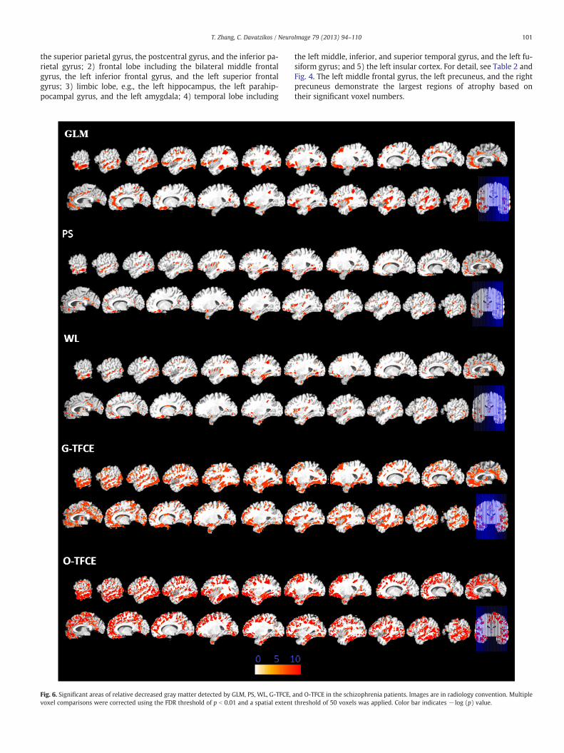
Fig. 6. Significant areas of relative decreased gray matter detected by GLM, PS, WL, G-TFCE,voxel comparisons were corrected using the FDR threshold of p b 0.01 and a spatial extent

the left middle, inferior, and superior temporal gyrus, and the left fu-siform gyrus; and 5) the left insular cortex. For detail, see Table 2 andFig. 4. The left middle frontal gyrus, the left precuneus, and the rightprecuneus demonstrate the largest regions of atrophy based ontheir significant voxel numbers.

and O-TFCE in the schizophrenia patients. Images are in radiology convention. Multiplethreshold of 50 voxels was applied. Color bar indicates − log (p) value.

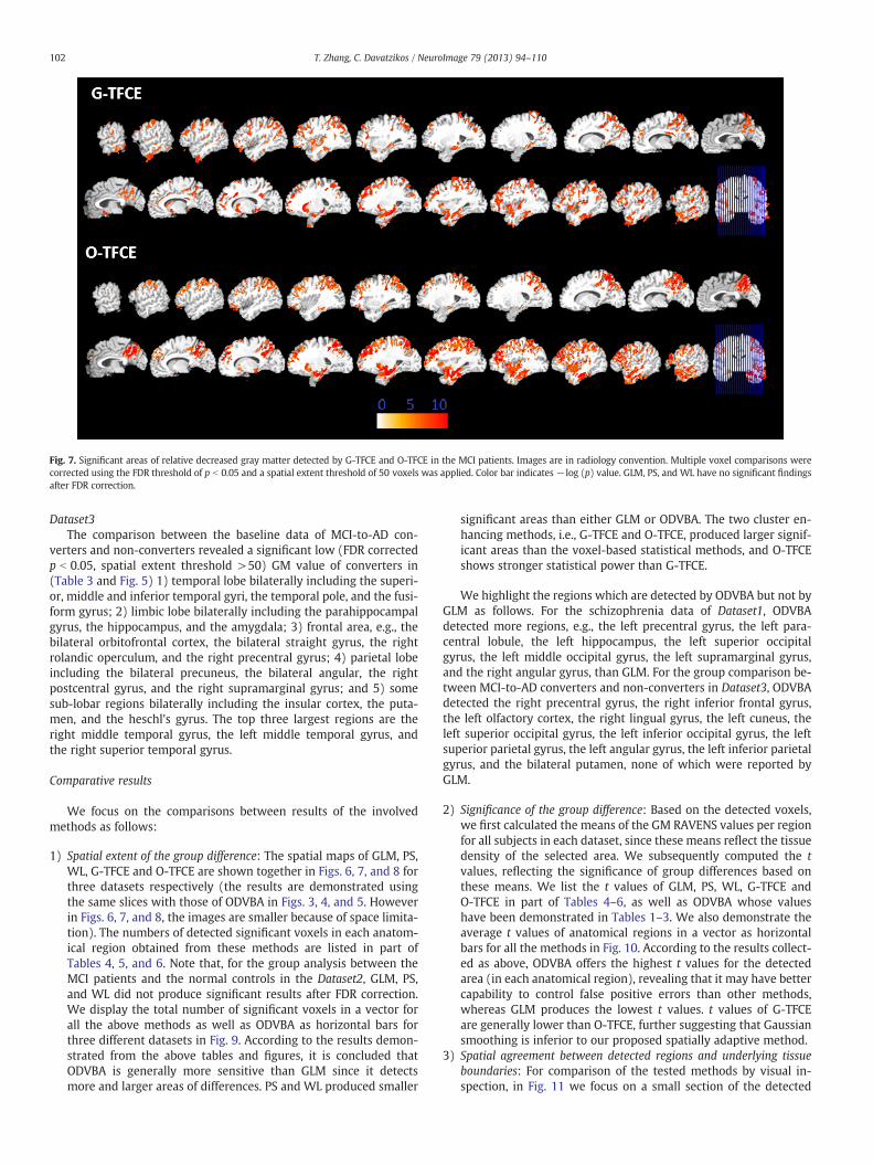
Fig. 7. Significant areas of relative decreased gray matter detected by G-TFCE and O-TFCE in the MCI patients. Images are in radiology convention. Multiple voxel comparisons werecorrected using the FDR threshold of p b 0.05 and a spatial extent threshold of 50 voxels was applied. Color bar indicates−log (p) value. GLM, PS, and WL have no significant findingsafter FDR correction.


Dataset3The comparison between the baseline data of MCI-to-AD con-

verters and non-converters revealed a significant low (FDR correctedp b 0.05, spatial extent threshold >50) GM value of converters in(Table 3 and Fig. 5) 1) temporal lobe bilaterally including the superi-or, middle and inferior temporal gyri, the temporal pole, and the fusi-form gyrus; 2) limbic lobe bilaterally including the parahippocampalgyrus, the hippocampus, and the amygdala; 3) frontal area, e.g., thebilateral orbitofrontal cortex, the bilateral straight gyrus, the rightrolandic operculum, and the right precentral gyrus; 4) parietal lobeincluding the bilateral precuneus, the bilateral angular, the rightpostcentral gyrus, and the right supramarginal gyrus; and 5) somesub-lobar regions bilaterally including the insular cortex, the puta-men, and the heschl's gyrus. The top three largest regions are theright middle temporal gyrus, the left middle temporal gyrus, andthe right superior temporal gyrus.

Comparative results

We focus on the comparisons between results of the involvedmethods as follows:

1) Spatial extent of the group difference: The spatial maps of GLM, PS,WL, G-TFCE and O-TFCE are shown together in Figs. 6, 7, and 8 forthree datasets respectively (the results are demonstrated usingthe same slices with those of ODVBA in Figs. 3, 4, and 5. Howeverin Figs. 6, 7, and 8, the images are smaller because of space limita-tion). The numbers of detected significant voxels in each anatom-ical region obtained from these methods are listed in part ofTables 4, 5, and 6. Note that, for the group analysis between theMCI patients and the normal controls in the Dataset2, GLM, PS,and WL did not produce significant results after FDR correction.We display the total number of significant voxels in a vector forall the above methods as well as ODVBA as horizontal bars forthree different datasets in Fig. 9. According to the results demon-strated from the above tables and figures, it is concluded thatODVBA is generally more sensitive than GLM since it detectsmore and larger areas of differences. PS and WL produced smaller

significant areas than either GLM or ODVBA. The two cluster en-hancing methods, i.e., G-TFCE and O-TFCE, produced larger signif-icant areas than the voxel-based statistical methods, and O-TFCEshows stronger statistical power than G-TFCE.

We highlight the regions which are detected by ODVBA but not byGLM as follows. For the schizophrenia data of Dataset1, ODVBAdetected more regions, e.g., the left precentral gyrus, the left para-central lobule, the left hippocampus, the left superior occipitalgyrus, the left middle occipital gyrus, the left supramarginal gyrus,and the right angular gyrus, than GLM. For the group comparison be-tween MCI-to-AD converters and non-converters in Dataset3, ODVBAdetected the right precentral gyrus, the right inferior frontal gyrus,the left olfactory cortex, the right lingual gyrus, the left cuneus, theleft superior occipital gyrus, the left inferior occipital gyrus, the leftsuperior parietal gyrus, the left angular gyrus, the left inferior parietalgyrus, and the bilateral putamen, none of which were reported byGLM.

2) Significance of the group difference: Based on the detected voxels,we first calculated the means of the GM RAVENS values per regionfor all subjects in each dataset, since these means reflect the tissuedensity of the selected area. We subsequently computed the tvalues, reflecting the significance of group differences based onthese means. We list the t values of GLM, PS, WL, G-TFCE andO-TFCE in part of Tables 4–6, as well as ODVBA whose valueshave been demonstrated in Tables 1–3. We also demonstrate theaverage t values of anatomical regions in a vector as horizontalbars for all the methods in Fig. 10. According to the results collect-ed as above, ODVBA offers the highest t values for the detectedarea (in each anatomical region), revealing that it may have bettercapability to control false positive errors than other methods,whereas GLM produces the lowest t values. t values of G-TFCEare generally lower than O-TFCE, further suggesting that Gaussiansmoothing is inferior to our proposed spatially adaptive method.

3) Spatial agreement between detected regions and underlying tissueboundaries: For comparison of the tested methods by visual in-spection, in Fig. 11 we focus on a small section of the detected

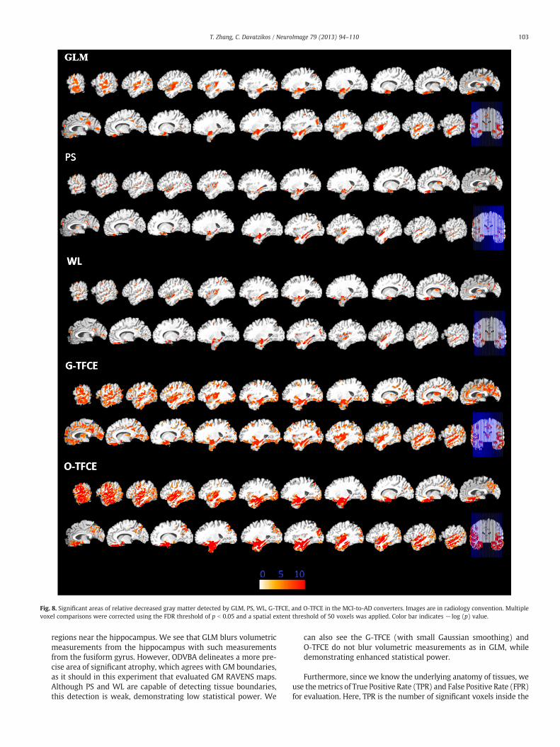
Fig. 8. Significant areas of relative decreased gray matter detected by GLM, PS, WL, G-TFCE, and O-TFCE in the MCI-to-AD converters. Images are in radiology convention. Multiplevoxel comparisons were corrected using the FDR threshold of p b 0.05 and a spatial extent threshold of 50 voxels was applied. Color bar indicates − log (p) value.


regions near the hippocampus. We see that GLM blurs volumetricmeasurements from the hippocampus with such measurementsfrom the fusiform gyrus. However, ODVBA delineates a more pre-cise area of significant atrophy, which agrees with GM boundaries,as it should in this experiment that evaluated GM RAVENS maps.Although PS and WL are capable of detecting tissue boundaries,this detection is weak, demonstrating low statistical power. We

can also see the G-TFCE (with small Gaussian smoothing) andO-TFCE do not blur volumetric measurements as in GLM, whiledemonstrating enhanced statistical power.

Furthermore, since we know the underlying anatomy of tissues, weuse themetrics of True Positive Rate (TPR) and False Positive Rate (FPR)for evaluation. Here, TPR is the number of significant voxels inside the

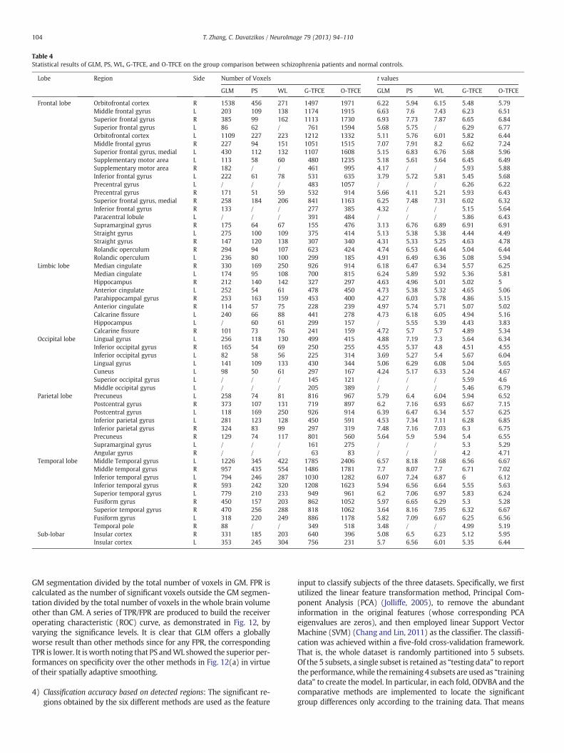
Table 4Statistical results of GLM, PS, WL, G-TFCE, and O-TFCE on the group comparison between schizophrenia patients and normal controls.

Lobe Region Side Number of Voxels t values

GLM PS WL G-TFCE O-TFCE GLM PS WL G-TFCE O-TFCE

Frontal lobe Orbitofrontal cortex R 1538 456 271 1497 1971 6.22 5.94 6.15 5.48 5.79Middle frontal gyrus L 203 109 138 1174 1915 6.63 7.6 7.43 6.23 6.51Superior frontal gyrus R 385 99 162 1113 1730 6.93 7.73 7.87 6.65 6.84Superior frontal gyrus L 86 62 / 761 1594 5.68 5.75 / 6.29 6.77Orbitofrontal cortex L 1109 227 223 1212 1332 5.11 5.76 6.01 5.82 6.44Middle frontal gyrus R 227 94 151 1051 1515 7.07 7.91 8.2 6.62 7.24Superior frontal gyrus, medial L 430 112 132 1107 1608 5.15 6.83 6.76 5.68 5.96Supplementary motor area L 113 58 60 480 1235 5.18 5.61 5.64 6.45 6.49Supplementary motor area R 182 / / 461 995 4.17 / / 5.93 5.88Inferior frontal gyrus L 222 61 78 531 635 3.79 5.72 5.81 5.45 5.68Precentral gyrus L / / / 483 1057 / / / 6.26 6.22Precentral gyrus R 171 51 59 532 914 5.66 4.11 5.21 5.93 6.43Superior frontal gyrus, medial R 258 184 206 841 1163 6.25 7.48 7.31 6.02 6.32Inferior frontal gyrus R 133 / / 277 385 4.32 / / 5.15 5.64Paracentral lobule L / / / 391 484 / / / 5.86 6.43Supramarginal gyrus R 175 64 67 155 476 3.13 6.76 6.89 6.91 6.91Straight gyrus L 275 100 109 375 414 5.13 5.38 5.38 4.44 4.49Straight gyrus R 147 120 138 307 340 4.31 5.33 5.25 4.63 4.78Rolandic operculum R 294 94 107 623 424 4.74 6.53 6.44 5.04 6.44Rolandic operculum L 236 80 100 299 185 4.91 6.49 6.36 5.08 5.94

Limbic lobe Median cingulate R 330 169 250 926 914 6.18 6.47 6.34 5.57 6.25Median cingulate L 174 95 108 700 815 6.24 5.89 5.92 5.36 5.81Hippocampus R 212 140 142 327 297 4.63 4.96 5.01 5.02 5Anterior cingulate L 252 54 61 478 450 4.73 5.38 5.32 4.65 5.06Parahippocampal gyrus R 253 163 159 453 400 4.27 6.03 5.78 4.86 5.15Anterior cingulate R 114 57 75 228 239 4.97 5.74 5.71 5.07 5.02Calcarine fissure L 240 66 88 441 278 4.73 6.18 6.05 4.94 5.16Hippocampus L / 60 61 299 157 / 5.55 5.39 4.43 3.83Calcarine fissure R 101 73 76 241 159 4.72 5.7 5.7 4.89 5.34

Occipital lobe Lingual gyrus L 256 118 130 499 415 4.88 7.19 7.3 5.64 6.34Inferior occipital gyrus R 165 54 69 250 255 4.55 5.37 4.8 4.51 4.55Inferior occipital gyrus L 82 58 56 225 314 3.69 5.27 5.4 5.67 6.04Lingual gyrus L 141 109 133 430 344 5.06 6.29 6.08 5.04 5.65Cuneus L 98 50 61 297 167 4.24 5.17 6.33 5.24 4.67Superior occipital gyrus L / / / 145 121 / / / 5.59 4.6Middle occipital gyrus L / / / 205 389 / / / 5.46 6.79

Parietal lobe Precuneus L 258 74 81 816 967 5.79 6.4 6.04 5.94 6.52Postcentral gyrus R 373 107 131 719 897 6.2 7.16 6.93 6.67 7.15Postcentral gyrus L 118 169 250 926 914 6.39 6.47 6.34 5.57 6.25Inferior parietal gyrus L 281 123 128 450 591 4.53 7.34 7.11 6.28 6.85Inferior parietal gyrus R 324 83 99 297 319 7.48 7.16 7.03 6.3 6.75Precuneus R 129 74 117 801 560 5.64 5.9 5.94 5.4 6.55Supramarginal gyrus L / / / 161 275 / / / 5.3 5.29Angular gyrus R / / / 63 83 / / / 4.2 4.71

Temporal lobe Middle Temporal gyrus L 1226 345 422 1785 2406 6.57 8.18 7.68 6.56 6.67Middle temporal gyrus R 957 435 554 1486 1781 7.7 8.07 7.7 6.71 7.02Inferior temporal gyrus L 794 246 287 1030 1282 6.07 7.24 6.87 6 6.12Inferior temporal gyrus R 593 242 320 1208 1623 5.94 6.56 6.64 5.55 5.63Superior temporal gyrus L 779 210 233 949 961 6.2 7.06 6.97 5.83 6.24Fusiform gyrus R 450 157 203 862 1052 5.97 6.65 6.29 5.3 5.28Superior temporal gyrus R 470 256 288 818 1062 3.64 8.16 7.95 6.32 6.67Fusiform gyrus L 318 220 249 886 1178 5.82 7.09 6.67 6.25 6.56Temporal pole R 88 / / 349 518 3.48 / / 4.99 5.19

Sub-lobar Insular cortex R 331 185 203 640 396 5.08 6.5 6.23 5.12 5.95Insular cortex L 353 245 304 756 231 5.7 6.56 6.01 5.35 6.44


GM segmentation divided by the total number of voxels in GM. FPR iscalculated as the number of significant voxels outside the GM segmen-tation divided by the total number of voxels in the whole brain volumeother than GM. A series of TPR/FPR are produced to build the receiveroperating characteristic (ROC) curve, as demonstrated in Fig. 12, byvarying the significance levels. It is clear that GLM offers a globallyworse result than other methods since for any FPR, the correspondingTPR is lower. It is worth noting that PS andWL showed the superior per-formances on specificity over the other methods in Fig. 12(a) in virtueof their spatially adaptive smoothing.

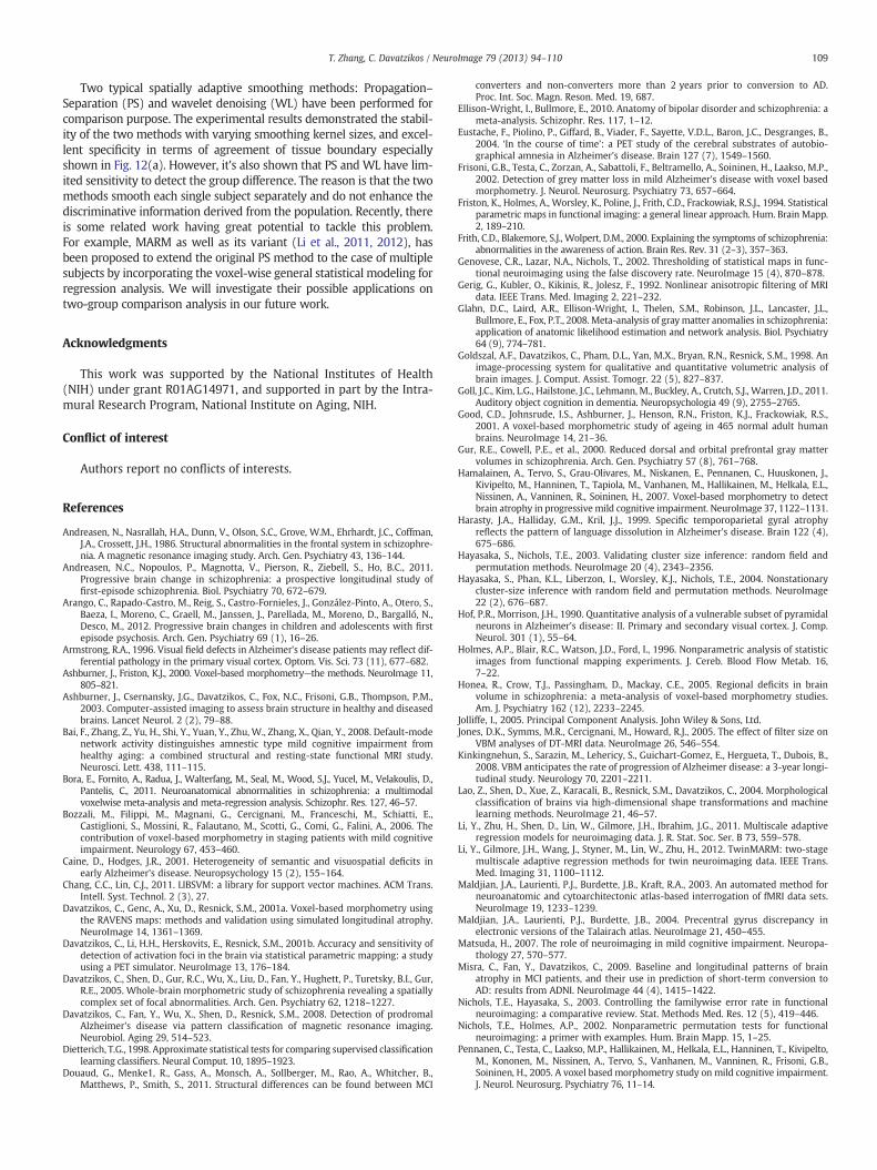
4) Classification accuracy based on detected regions: The significant re-gions obtained by the six different methods are used as the feature

input to classify subjects of the three datasets. Specifically, we firstutilized the linear feature transformation method, Principal Com-ponent Analysis (PCA) (Jolliffe, 2005), to remove the abundantinformation in the original features (whose corresponding PCAeigenvalues are zeros), and then employed linear Support VectorMachine (SVM) (Chang and Lin, 2011) as the classifier. The classifi-cation was achieved within a five-fold cross-validation framework.That is, the whole dataset is randomly partitioned into 5 subsets.Of the 5 subsets, a single subset is retained as “testing data” to reportthe performance,while the remaining4 subsets are used as “trainingdata” to create the model. In particular, in each fold, ODVBA and thecomparative methods are implemented to locate the significantgroup differences only according to the training data. That means

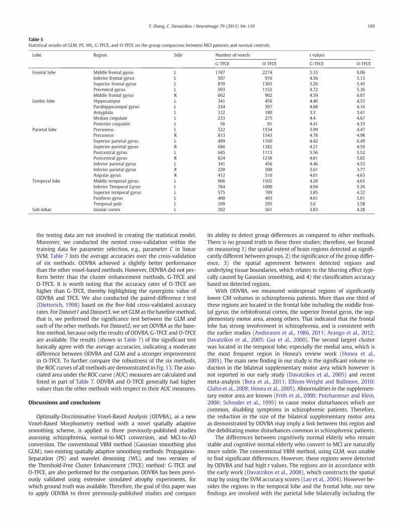
Table 5Statistical results of GLM, PS, WL, G-TFCE, and O-TFCE on the group comparison between MCI patients and normal controls.

Lobe Region Side Number of voxels t values

G-TFCE O-TFCE G-TFCE O-TFCE

Frontal lobe Middle frontal gyrus L 1187 2274 5.33 6.06Inferior frontal gyrus L 507 910 4.56 5.13Superior frontal gyrus L 870 1303 5.26 5.45Precentral gyrus L 503 1152 4.72 5.36Middle frontal gyrus R 662 962 4.59 6.07

Limbic lobe Hippocampus L 341 456 4.46 4.53Parahippocampal gyrus L 234 397 4.68 4.16Amygdala L 122 180 3.3 3.41Median cingulate L 233 275 4.4 4.67Posterior cingulate L 56 81 4.41 4.33

Parietal lobe Precuneus L 522 1534 3.99 4.47Precuneus R 813 1543 4.78 4.98Superior parietal gyrus L 499 1160 4.42 6.49Superior parietal gyrus R 686 1382 4.21 4.59Postcentral gyrus L 645 1113 5.56 5.52Postcentral gyrus R 824 1238 4.81 5.65Inferior parietal gyrus L 341 456 4.46 4.53Inferior parietal gyrus R 220 508 3.61 3.77Angular gyrus R 412 510 4.01 4.63

Temporal lobe Middle temporal gyrus L 966 1502 4.26 4.63Inferior Temporal Gyrus L 784 1000 4.94 5.26Superior temporal gyrus L 575 789 3.85 4.32Fusiform gyrus L 400 493 4.61 5.01Temporal pole L 109 295 3.6 3.58

Sub-lobar Insular cortex L 392 561 3.83 4.28


the testing data are not involved in creating the statistical model.Moreover, we conducted the nested cross-validation within thetraining data for parameter selection, e.g., parameter C in linearSVM. Table 7 lists the average accuracies over the cross-validationof six methods. ODVBA achieved a slightly better performancethan the other voxel-based methods. However, ODVBA did not per-form better than the cluster enhancement methods, G-TFCE andO-TFCE. It is worth noting that the accuracy rates of O-TFCE arehigher than G-TFCE, thereby highlighting the synergistic value ofODVBA and TFCE. We also conducted the paired-difference t test(Dietterich, 1998) based on the five-fold cross-validated accuracyrates. ForDataset1 andDataset3, we set GLMas the baselinemethod,that is, we performed the significance test between the GLM andeach of the other methods. For Dataset2, we set ODVBA as the base-linemethod, because only the results of ODVBA, G-TFCE and O-TFCEare available. The results (shown in Table 7) of the significant testbasically agree with the average accuracies, indicating a moderatedifference between ODVBA and GLM and a stronger improvementin O-TFCE. To further compare the robustness of the six methods,the ROC curves of all methods are demonstrated in Fig. 13. The asso-ciated area under the ROC curve (AUC) measures are calculated andlisted in part of Table 7. ODVBA and O-TFCE generally had highervalues than the other methods with respect to their AUC measures.

Discussions and conclusions

Optimally-Discriminative Voxel-Based Analysis (ODVBA), as a newVoxel-Based Morphometry method with a novel spatially adaptivesmoothing scheme, is applied to three previously-published studiesassessing schizophrenia, normal-to-MCI conversion, and MCI-to-ADconversion. The conventional VBM method (Gaussian smoothing plusGLM), two existing spatially adaptive smoothing methods: Propagation-Separation (PS) and wavelet denoising (WL), and two versions ofthe Threshold-Free Cluster Enhancement (TFCE) method: G-TFCE andO-TFCE, are also performed for the comparison. ODVBA has been previ-ously validated using extensive simulated atrophy experiments, forwhich ground truth was available. Therefore, the goal of this paper wasto apply ODVBA to three previously-published studies and compare

its ability to detect group differences as compared to other methods.There is no ground truth in these three studies; therefore, we focusedon measuring 1) the spatial extent of brain regions detected as signifi-cantly different between groups, 2) the significance of the group differ-ence, 3) the spatial agreement between detected regions andunderlying tissue boundaries, which relates to the blurring effect typi-cally caused by Gaussian smoothing, and 4) the classification accuracybased on detected regions.

With ODVBA, we measured widespread regions of significantlylower GM volumes in schizophrenia patients. More than one third ofthese regions are located in the frontal lobe including the middle fron-tal gyrus, the orbitofrontal cortex, the superior frontal gyrus, the sup-plementary motor area, among others. That indicated that the frontallobe has strong involvement in schizophrenia, and is consistent withthe earlier studies (Andreasen et al., 1986, 2011; Arango et al., 2012;Davatzikos et al., 2005; Gur et al., 2000). The second largest clusterwas located in the temporal lobe, especially the medial area, which isthe most frequent region in Honea's review work (Honea et al.,2005). The main new finding in our study is the significant volume re-duction in the bilateral supplementary motor area which however isnot reported in our early study (Davatzikos et al., 2005) and recentmeta-analysis (Bora et al., 2011; Ellison-Wright and Bullmore, 2010;Glahn et al., 2008; Honea et al., 2005). Abnormalities in the supplemen-tary motor area are known (Frith et al., 2000; Putzhammer and Klein,2006; Schroder et al., 1995) to cause motor disturbances which arecommon, disabling symptoms in schizophrenic patients. Therefore,the reduction in the size of the bilateral supplementary motor areaas demonstrated by ODVBA may imply a link between this region andthe debilitating motor disturbances common in schizophrenic patients.

The differences between cognitively normal elderly who remainstable and cognitive normal elderly who convert to MCI are naturallymore subtle. The conventional VBM method, using GLM, was unableto find significant differences. However, these regions were detectedby ODVBA and had high t values. The regions are in accordance withthe early work (Davatzikos et al., 2008), which constructs the spatialmap by using the SVM accuracy scores (Lao et al., 2004). However be-sides the regions in the temporal lobe and the frontal lobe, our newfindings are involved with the parietal lobe bilaterally including the

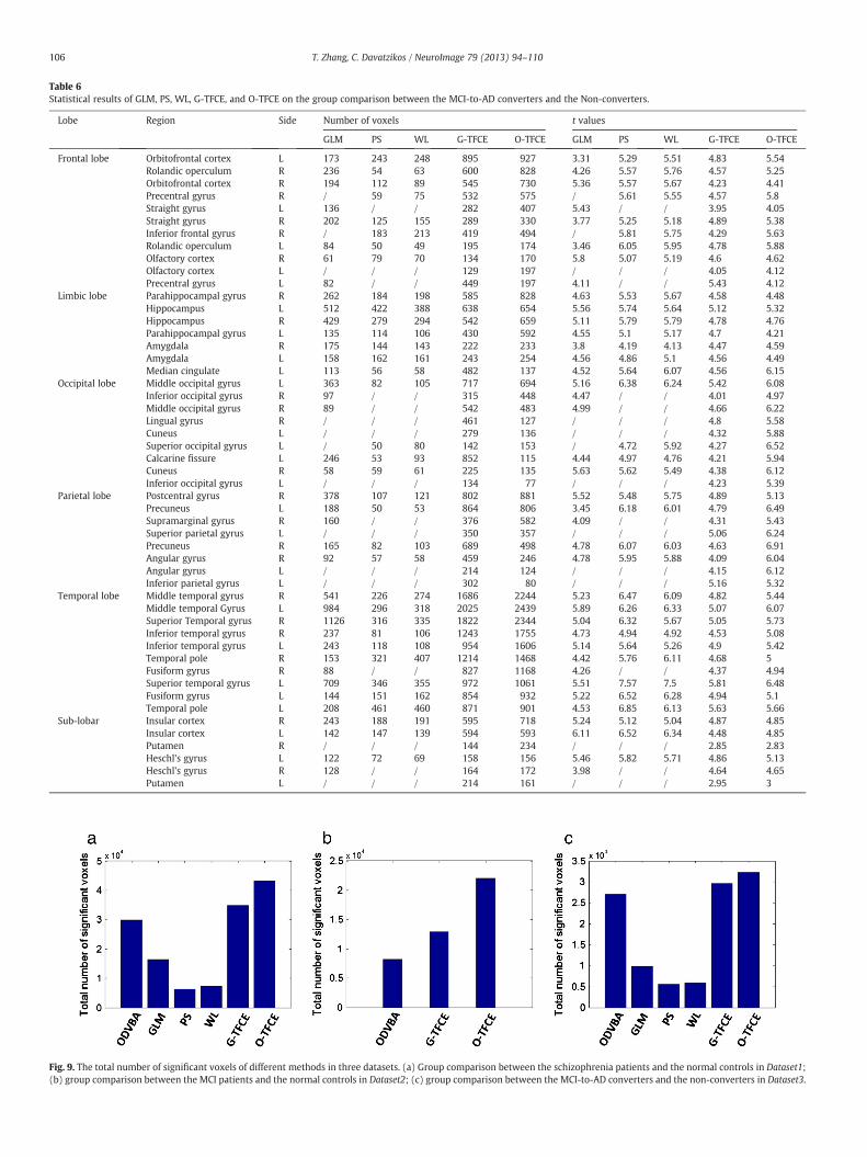
Table 6Statistical results of GLM, PS, WL, G-TFCE, and O-TFCE on the group comparison between the MCI-to-AD converters and the Non-converters.

Lobe Region Side Number of voxels t values

GLM PS WL G-TFCE O-TFCE GLM PS WL G-TFCE O-TFCE

Frontal lobe Orbitofrontal cortex L 173 243 248 895 927 3.31 5.29 5.51 4.83 5.54Rolandic operculum R 236 54 63 600 828 4.26 5.57 5.76 4.57 5.25Orbitofrontal cortex R 194 112 89 545 730 5.36 5.57 5.67 4.23 4.41Precentral gyrus R / 59 75 532 575 / 5.61 5.55 4.57 5.8Straight gyrus L 136 / / 282 407 5.43 / / 3.95 4.05Straight gyrus R 202 125 155 289 330 3.77 5.25 5.18 4.89 5.38Inferior frontal gyrus R / 183 213 419 494 / 5.81 5.75 4.29 5.63Rolandic operculum L 84 50 49 195 174 3.46 6.05 5.95 4.78 5.88Olfactory cortex R 61 79 70 134 170 5.8 5.07 5.19 4.6 4.62Olfactory cortex L / / / 129 197 / / / 4.05 4.12Precentral gyrus L 82 / / 449 197 4.11 / / 5.43 4.12

Limbic lobe Parahippocampal gyrus R 262 184 198 585 828 4.63 5.53 5.67 4.58 4.48Hippocampus L 512 422 388 638 654 5.56 5.74 5.64 5.12 5.32Hippocampus R 429 279 294 542 659 5.11 5.79 5.79 4.78 4.76Parahippocampal gyrus L 135 114 106 430 592 4.55 5.1 5.17 4.7 4.21Amygdala R 175 144 143 222 233 3.8 4.19 4.13 4.47 4.59Amygdala L 158 162 161 243 254 4.56 4.86 5.1 4.56 4.49Median cingulate L 113 56 58 482 137 4.52 5.64 6.07 4.56 6.15

Occipital lobe Middle occipital gyrus L 363 82 105 717 694 5.16 6.38 6.24 5.42 6.08Inferior occipital gyrus R 97 / / 315 448 4.47 / / 4.01 4.97Middle occipital gyrus R 89 / / 542 483 4.99 / / 4.66 6.22Lingual gyrus R / / / 461 127 / / / 4.8 5.58Cuneus L / / / 279 136 / / / 4.32 5.88Superior occipital gyrus L / 50 80 142 153 / 4.72 5.92 4.27 6.52Calcarine fissure L 246 53 93 852 115 4.44 4.97 4.76 4.21 5.94Cuneus R 58 59 61 225 135 5.63 5.62 5.49 4.38 6.12Inferior occipital gyrus L / / / 134 77 / / / 4.23 5.39

Parietal lobe Postcentral gyrus R 378 107 121 802 881 5.52 5.48 5.75 4.89 5.13Precuneus L 188 50 53 864 806 3.45 6.18 6.01 4.79 6.49Supramarginal gyrus R 160 / / 376 582 4.09 / / 4.31 5.43Superior parietal gyrus L / / / 350 357 / / / 5.06 6.24Precuneus R 165 82 103 689 498 4.78 6.07 6.03 4.63 6.91Angular gyrus R 92 57 58 459 246 4.78 5.95 5.88 4.09 6.04Angular gyrus L / / / 214 124 / / / 4.15 6.12Inferior parietal gyrus L / / / 302 80 / / / 5.16 5.32

Temporal lobe Middle temporal gyrus R 541 226 274 1686 2244 5.23 6.47 6.09 4.82 5.44Middle temporal Gyrus L 984 296 318 2025 2439 5.89 6.26 6.33 5.07 6.07Superior Temporal gyrus R 1126 316 335 1822 2344 5.04 6.32 5.67 5.05 5.73Inferior temporal gyrus R 237 81 106 1243 1755 4.73 4.94 4.92 4.53 5.08Inferior temporal gyrus L 243 118 108 954 1606 5.14 5.64 5.26 4.9 5.42Temporal pole R 153 321 407 1214 1468 4.42 5.76 6.11 4.68 5Fusiform gyrus R 88 / / 827 1168 4.26 / / 4.37 4.94Superior temporal gyrus L 709 346 355 972 1061 5.51 7.57 7.5 5.81 6.48Fusiform gyrus L 144 151 162 854 932 5.22 6.52 6.28 4.94 5.1Temporal pole L 208 461 460 871 901 4.53 6.85 6.13 5.63 5.66

Sub-lobar Insular cortex R 243 188 191 595 718 5.24 5.12 5.04 4.87 4.85Insular cortex L 142 147 139 594 593 6.11 6.52 6.34 4.48 4.85Putamen R / / / 144 234 / / / 2.85 2.83Heschl's gyrus L 122 72 69 158 156 5.46 5.82 5.71 4.86 5.13Heschl's gyrus R 128 / / 164 172 3.98 / / 4.64 4.65Putamen L / / / 214 161 / / / 2.95 3

Fig. 9. The total number of significant voxels of different methods in three datasets. (a) Group comparison between the schizophrenia patients and the normal controls in Dataset1;(b) group comparison between the MCI patients and the normal controls in Dataset2; (c) group comparison between the MCI-to-AD converters and the non-converters in Dataset3.


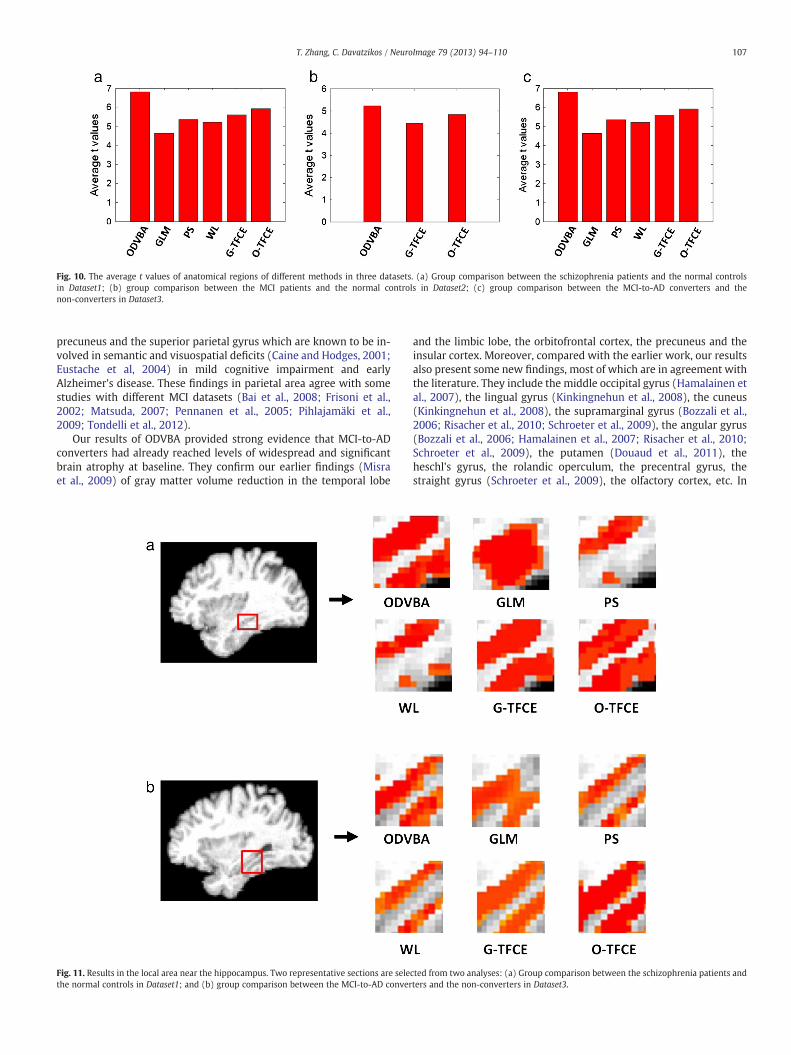
Fig. 10. The average t values of anatomical regions of different methods in three datasets. (a) Group comparison between the schizophrenia patients and the normal controlsin Dataset1; (b) group comparison between the MCI patients and the normal controls in Dataset2; (c) group comparison between the MCI-to-AD converters and thenon-converters in Dataset3.


precuneus and the superior parietal gyrus which are known to be in-volved in semantic and visuospatial deficits (Caine and Hodges, 2001;Eustache et al, 2004) in mild cognitive impairment and earlyAlzheimer's disease. These findings in parietal area agree with somestudies with different MCI datasets (Bai et al., 2008; Frisoni et al.,2002; Matsuda, 2007; Pennanen et al., 2005; Pihlajamäki et al.,2009; Tondelli et al., 2012).

Our results of ODVBA provided strong evidence that MCI-to-ADconverters had already reached levels of widespread and significantbrain atrophy at baseline. They confirm our earlier findings (Misraet al., 2009) of gray matter volume reduction in the temporal lobe

Fig. 11. Results in the local area near the hippocampus. Two representative sections are selethe normal controls in Dataset1; and (b) group comparison between the MCI-to-AD conver

and the limbic lobe, the orbitofrontal cortex, the precuneus and theinsular cortex. Moreover, compared with the earlier work, our resultsalso present some new findings, most of which are in agreement withthe literature. They include the middle occipital gyrus (Hamalainen etal., 2007), the lingual gyrus (Kinkingnehun et al., 2008), the cuneus(Kinkingnehun et al., 2008), the supramarginal gyrus (Bozzali et al.,2006; Risacher et al., 2010; Schroeter et al., 2009), the angular gyrus(Bozzali et al., 2006; Hamalainen et al., 2007; Risacher et al., 2010;Schroeter et al., 2009), the putamen (Douaud et al., 2011), theheschl's gyrus, the rolandic operculum, the precentral gyrus, thestraight gyrus (Schroeter et al., 2009), the olfactory cortex, etc. In

cted from two analyses: (a) Group comparison between the schizophrenia patients andters and the non-converters in Dataset3.

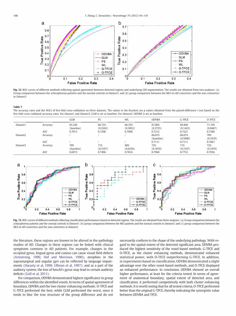
Fig. 12. ROC curves of different methods reflecting spatial agreement between detected regions and underlying GM segmentation. The results are obtained from two analyses: (a)Group comparison between the schizophrenia patients and the normal controls in Dataset1; and (b) group comparison between the MCI-to-AD converters and the non-convertersin Dataset3.

Table 7The accuracy rates and the AUCs of five-fold cross-validation on three datasets. The values in the brackets are p values obtained from the paired-difference t test based on thefive-fold cross-validated accuracy rates. For Dataset1 and Dataset3, GLM is set as baseline. For Dataset2, ODVBA is set as baseline.

GLM PS WL ODVBA G-TFCE O-TFCE

Dataset1 Accuracy 65.24%(baseline)

66.75%(0.3262)

66.35%(0.3852)

67.06%(0.3725)

69.44%(0.1422)

71.19%(0.0467)

AUC 0.7013 0.7298 0.7090 0.7212 0.7221 0.7386Dataset2 Accuracy / / / 66.67%

(baseline)66.67%(0.5000)

70%(0.1870)

AUC / / / 0.7111 0.7111 0.7867Dataset3 Accuracy 70%

(baseline)71%(0.3107)

68%(0.6256)

72%(0.1870)

71%(0.3107)

72%(0.1870)

AUC 0.6972 0.7496 0.7816 0.7960 0.7752 0.7956

Fig. 13. ROC curves of differentmethods reflecting classification performances based on detected regions. The results are obtained from three analyses: (a) Group comparison between theschizophrenia patients and the normal controls in Dataset1; (b) group comparison between the MCI patients and the normal controls in Dataset2; and (c) group comparison between theMCI-to-AD converters and the non-converters in Dataset3.


the literature, these regions are known to be altered in the pathologystudies of AD. Changes in these regions can be linked with clinicalsymptoms common in AD patients. For example, changes in theoccipital gyrus, lingual gyrus and cuneus can cause visual field defects(Armstrong, 1996; Hof and Morrison, 1990); atrophies in thesupramarginal and angular gyri can be reflected by language impair-ments (Harasty et al, 1999; Ullman et al, 1997); and as a part of theauditory system, the loss of heschl's gyrus may lead to certain auditorydeficits (Goll et al, 2011).

For comparison, ODVBA demonstrated highest significance in groupdifferenceswithin the identified voxels. In terms of spatial agreement ofboundary, ODVBA and the two cluster enhancingmethods: O-TFCE andG-TFCE performed the best, while GLM performed the worst, since ittends to blur the true structure of the group difference and do not

necessarily conform to the shape of the underlying pathology. With re-gard to the spatial extent of the detected significant area, ODVBA pro-duced the highest sensitivity of the voxel-based methods. G-TFCE andO-TFCE, as the cluster enhancing methods, demonstrated enhancedstatistical power, with O-TFCE outperforming G-TFCE. In addition,in experiments based on classification, ODVBA demonstrated a slightadvantage over the other voxel-based methods, and O-TFCE displayedan enhanced performance. In conclusion, ODVBA showed an overallhigher performance, at least for the criteria tested. In terms of agree-ment of anatomical boundary, spatial extent of detected area, andclassification, it performed competitively with both cluster enhancingmethods. It is worth noting that for all tested criteria, O-TFCE performedbetter than the original G-TFCE, thereby indicating the synergistic valuebetween ODVBA and TFCE.


Two typical spatially adaptive smoothing methods: Propagation–Separation (PS) and wavelet denoising (WL) have been performed forcomparison purpose. The experimental results demonstrated the stabil-ity of the two methods with varying smoothing kernel sizes, and excel-lent specificity in terms of agreement of tissue boundary especiallyshown in Fig. 12(a). However, it's also shown that PS and WL have lim-ited sensitivity to detect the group difference. The reason is that the twomethods smooth each single subject separately and do not enhance thediscriminative information derived from the population. Recently, thereis some related work having great potential to tackle this problem.For example, MARM as well as its variant (Li et al., 2011, 2012), hasbeen proposed to extend the original PS method to the case of multiplesubjects by incorporating the voxel-wise general statistical modeling forregression analysis. We will investigate their possible applications ontwo-group comparison analysis in our future work.

Acknowledgments

This work was supported by the National Institutes of Health(NIH) under grant R01AG14971, and supported in part by the Intra-mural Research Program, National Institute on Aging, NIH.

Conflict of interest

Authors report no conflicts of interests.

References

Andreasen, N., Nasrallah, H.A., Dunn, V., Olson, S.C., Grove, W.M., Ehrhardt, J.C., Coffman,J.A., Crossett, J.H., 1986. Structural abnormalities in the frontal system in schizophre-nia. A magnetic resonance imaging study. Arch. Gen. Psychiatry 43, 136–144.

Andreasen, N.C., Nopoulos, P., Magnotta, V., Pierson, R., Ziebell, S., Ho, B.C., 2011.Progressive brain change in schizophrenia: a prospective longitudinal study offirst-episode schizophrenia. Biol. Psychiatry 70, 672–679.

Arango, C., Rapado-Castro, M., Reig, S., Castro-Fornieles, J., González-Pinto, A., Otero, S.,Baeza, I., Moreno, C., Graell, M., Janssen, J., Parellada, M., Moreno, D., Bargalló, N.,Desco, M., 2012. Progressive brain changes in children and adolescents with firstepisode psychosis. Arch. Gen. Psychiatry 69 (1), 16–26.

Armstrong, R.A., 1996. Visual field defects in Alzheimer's disease patients may reflect dif-ferential pathology in the primary visual cortex. Optom. Vis. Sci. 73 (11), 677–682.

Ashburner, J., Friston, K.J., 2000. Voxel-based morphometry—the methods. NeuroImage 11,805–821.

Ashburner, J., Csernansky, J.G., Davatzikos, C., Fox, N.C., Frisoni, G.B., Thompson, P.M.,2003. Computer-assisted imaging to assess brain structure in healthy and diseasedbrains. Lancet Neurol. 2 (2), 79–88.

Bai, F., Zhang, Z., Yu, H., Shi, Y., Yuan, Y., Zhu, W., Zhang, X., Qian, Y., 2008. Default-modenetwork activity distinguishes amnestic type mild cognitive impairment fromhealthy aging: a combined structural and resting-state functional MRI study.Neurosci. Lett. 438, 111–115.

Bora, E., Fornito, A., Radua, J., Walterfang, M., Seal, M., Wood, S.J., Yucel, M., Velakoulis, D.,Pantelis, C., 2011. Neuroanatomical abnormalities in schizophrenia: a multimodalvoxelwise meta-analysis and meta-regression analysis. Schizophr. Res. 127, 46–57.

Bozzali, M., Filippi, M., Magnani, G., Cercignani, M., Franceschi, M., Schiatti, E.,Castiglioni, S., Mossini, R., Falautano, M., Scotti, G., Comi, G., Falini, A., 2006. Thecontribution of voxel-based morphometry in staging patients with mild cognitiveimpairment. Neurology 67, 453–460.

Caine, D., Hodges, J.R., 2001. Heterogeneity of semantic and visuospatial deficits inearly Alzheimer's disease. Neuropsychology 15 (2), 155–164.

Chang, C.C., Lin, C.J., 2011. LIBSVM: a library for support vector machines. ACM Trans.Intell. Syst. Technol. 2 (3), 27.

Davatzikos, C., Genc, A., Xu, D., Resnick, S.M., 2001a. Voxel-based morphometry usingthe RAVENS maps: methods and validation using simulated longitudinal atrophy.NeuroImage 14, 1361–1369.

Davatzikos, C., Li, H.H., Herskovits, E., Resnick, S.M., 2001b. Accuracy and sensitivity ofdetection of activation foci in the brain via statistical parametric mapping: a studyusing a PET simulator. NeuroImage 13, 176–184.

Davatzikos, C., Shen, D., Gur, R.C., Wu, X., Liu, D., Fan, Y., Hughett, P., Turetsky, B.I., Gur,R.E., 2005. Whole-brain morphometric study of schizophrenia revealing a spatiallycomplex set of focal abnormalities. Arch. Gen. Psychiatry 62, 1218–1227.

Davatzikos, C., Fan, Y., Wu, X., Shen, D., Resnick, S.M., 2008. Detection of prodromalAlzheimer's disease via pattern classification of magnetic resonance imaging.Neurobiol. Aging 29, 514–523.

Dietterich, T.G., 1998. Approximate statistical tests for comparing supervised classificationlearning classifiers. Neural Comput. 10, 1895–1923.

Douaud, G., Menke1, R., Gass, A., Monsch, A., Sollberger, M., Rao, A., Whitcher, B.,Matthews, P., Smith, S., 2011. Structural differences can be found between MCI

converters and non-converters more than 2 years prior to conversion to AD.Proc. Int. Soc. Magn. Reson. Med. 19, 687.

Ellison-Wright, I., Bullmore, E., 2010. Anatomy of bipolar disorder and schizophrenia: ameta-analysis. Schizophr. Res. 117, 1–12.

Eustache, F., Piolino, P., Giffard, B., Viader, F., Sayette, V.D.L., Baron, J.C., Desgranges, B.,2004. ‘In the course of time’: a PET study of the cerebral substrates of autobio-graphical amnesia in Alzheimer's disease. Brain 127 (7), 1549–1560.

Frisoni, G.B., Testa, C., Zorzan, A., Sabattoli, F., Beltramello, A., Soininen, H., Laakso, M.P.,2002. Detection of grey matter loss in mild Alzheimer's disease with voxel basedmorphometry. J. Neurol. Neurosurg. Psychiatry 73, 657–664.

Friston, K., Holmes, A., Worsley, K., Poline, J., Frith, C.D., Frackowiak, R.S.J., 1994. Statisticalparametric maps in functional imaging: a general linear approach. Hum. Brain Mapp.2, 189–210.

Frith, C.D., Blakemore, S.J., Wolpert, D.M., 2000. Explaining the symptoms of schizophrenia:abnormalities in the awareness of action. Brain Res. Rev. 31 (2–3), 357–363.

Genovese, C.R., Lazar, N.A., Nichols, T., 2002. Thresholding of statistical maps in func-tional neuroimaging using the false discovery rate. NeuroImage 15 (4), 870–878.

Gerig, G., Kubler, O., Kikinis, R., Jolesz, F., 1992. Nonlinear anisotropic filtering of MRIdata. IEEE Trans. Med. Imaging 2, 221–232.

Glahn, D.C., Laird, A.R., Ellison-Wright, I., Thelen, S.M., Robinson, J.L., Lancaster, J.L.,Bullmore, E., Fox, P.T., 2008. Meta-analysis of graymatter anomalies in schizophrenia:application of anatomic likelihood estimation and network analysis. Biol. Psychiatry64 (9), 774–781.

Goldszal, A.F., Davatzikos, C., Pham, D.L., Yan, M.X., Bryan, R.N., Resnick, S.M., 1998. Animage-processing system for qualitative and quantitative volumetric analysis ofbrain images. J. Comput. Assist. Tomogr. 22 (5), 827–837.

Goll, J.C., Kim, L.G., Hailstone, J.C., Lehmann, M., Buckley, A., Crutch, S.J., Warren, J.D., 2011.Auditory object cognition in dementia. Neuropsychologia 49 (9), 2755–2765.

Good, C.D., Johnsrude, I.S., Ashburner, J., Henson, R.N., Friston, K.J., Frackowiak, R.S.,2001. A voxel-based morphometric study of ageing in 465 normal adult humanbrains. NeuroImage 14, 21–36.

Gur, R.E., Cowell, P.E., et al., 2000. Reduced dorsal and orbital prefrontal gray mattervolumes in schizophrenia. Arch. Gen. Psychiatry 57 (8), 761–768.

Hamalainen, A., Tervo, S., Grau-Olivares, M., Niskanen, E., Pennanen, C., Huuskonen, J.,Kivipelto, M., Hanninen, T., Tapiola, M., Vanhanen, M., Hallikainen, M., Helkala, E.L.,Nissinen, A., Vanninen, R., Soininen, H., 2007. Voxel-based morphometry to detectbrain atrophy in progressive mild cognitive impairment. NeuroImage 37, 1122–1131.

Harasty, J.A., Halliday, G.M., Kril, J.J., 1999. Specific temporoparietal gyral atrophyreflects the pattern of language dissolution in Alzheimer's disease. Brain 122 (4),675–686.

Hayasaka, S., Nichols, T.E., 2003. Validating cluster size inference: random field andpermutation methods. NeuroImage 20 (4), 2343–2356.

Hayasaka, S., Phan, K.L., Liberzon, I., Worsley, K.J., Nichols, T.E., 2004. Nonstationarycluster-size inference with random field and permutation methods. NeuroImage22 (2), 676–687.

Hof, P.R., Morrison, J.H., 1990. Quantitative analysis of a vulnerable subset of pyramidalneurons in Alzheimer's disease: II. Primary and secondary visual cortex. J. Comp.Neurol. 301 (1), 55–64.

Holmes, A.P., Blair, R.C., Watson, J.D., Ford, I., 1996. Nonparametric analysis of statisticimages from functional mapping experiments. J. Cereb. Blood Flow Metab. 16,7–22.

Honea, R., Crow, T.J., Passingham, D., Mackay, C.E., 2005. Regional deficits in brainvolume in schizophrenia: a meta-analysis of voxel-based morphometry studies.Am. J. Psychiatry 162 (12), 2233–2245.

Jolliffe, I., 2005. Principal Component Analysis. John Wiley & Sons, Ltd.Jones, D.K., Symms, M.R., Cercignani, M., Howard, R.J., 2005. The effect of filter size on

VBM analyses of DT-MRI data. NeuroImage 26, 546–554.Kinkingnehun, S., Sarazin, M., Lehericy, S., Guichart-Gomez, E., Hergueta, T., Dubois, B.,

2008. VBM anticipates the rate of progression of Alzheimer disease: a 3-year longi-tudinal study. Neurology 70, 2201–2211.

Lao, Z., Shen, D., Xue, Z., Karacali, B., Resnick, S.M., Davatzikos, C., 2004. Morphologicalclassification of brains via high-dimensional shape transformations and machinelearning methods. NeuroImage 21, 46–57.

Li, Y., Zhu, H., Shen, D., Lin, W., Gilmore, J.H., Ibrahim, J.G., 2011. Multiscale adaptiveregression models for neuroimaging data. J. R. Stat. Soc. Ser. B 73, 559–578.

Li, Y., Gilmore, J.H., Wang, J., Styner, M., Lin, W., Zhu, H., 2012. TwinMARM: two-stagemultiscale adaptive regression methods for twin neuroimaging data. IEEE Trans.Med. Imaging 31, 1100–1112.

Maldjian, J.A., Laurienti, P.J., Burdette, J.B., Kraft, R.A., 2003. An automated method forneuroanatomic and cytoarchitectonic atlas-based interrogation of fMRI data sets.NeuroImage 19, 1233–1239.

Maldjian, J.A., Laurienti, P.J., Burdette, J.B., 2004. Precentral gyrus discrepancy inelectronic versions of the Talairach atlas. NeuroImage 21, 450–455.

Matsuda, H., 2007. The role of neuroimaging in mild cognitive impairment. Neuropa-thology 27, 570–577.

Misra, C., Fan, Y., Davatzikos, C., 2009. Baseline and longitudinal patterns of brainatrophy in MCI patients, and their use in prediction of short-term conversion toAD: results from ADNI. NeuroImage 44 (4), 1415–1422.

Nichols, T.E., Hayasaka, S., 2003. Controlling the familywise error rate in functionalneuroimaging: a comparative review. Stat. Methods Med. Res. 12 (5), 419–446.

Nichols, T.E., Holmes, A.P., 2002. Nonparametric permutation tests for functionalneuroimaging: a primer with examples. Hum. Brain Mapp. 15, 1–25.

Pennanen, C., Testa, C., Laakso, M.P., Hallikainen, M., Helkala, E.L., Hanninen, T., Kivipelto,M., Kononen, M., Nissinen, A., Tervo, S., Vanhanen, M., Vanninen, R., Frisoni, G.B.,Soininen, H., 2005. A voxel based morphometry study on mild cognitive impairment.J. Neurol. Neurosurg. Psychiatry 76, 11–14.


Perona, P., Malik, J., 1990. Scale-space and edge detection using anisotropic diffusion.IEEE Trans. Pattern Anal. Mach. Intell. 12 (7), 629–663.

Pihlajamäki, M., Jauhiainen, A.M., Soininen, H., 2009. Structural and functional MRI inmild cognitive impairment. Curr. Alzheimer Res. 6, 179–185.

Pizurica, A., Philips, W., Lemahieu, I., Acheroy, M., 2003. A versatile wavelet domain noisefiltration technique for medical imaging. IEEE Trans. Med. Imaging 22, 323–331.

Polzehl, J., Spokoiny, V., 2000. Adaptive weights smoothing with applications to imagerestoration. J. R. Stat. Soc. Ser. B 62, 335–354.

Polzehl, J., Spokoiny, V., 2006. Local likelihood modeling by adaptive weights smooth-ing. Probab. Theory Relat. Fields 135, 335–362.

Putzhammer, A., Klein, H.E., 2006. Quantitative analysis of motor disturbances inschizophrenic patients. Dialogues Clin. Neurosci. 8 (1), 123–130.

Risacher, S.L., Shen, L., West, J.D., Kim, S., McDonald, B.C., Beckett, L.A., Harvey, D.J., Jack,C.R., Weiner, M.W., Saykin, A.J., 2010. Longitudinal MRI atrophy biomarkers:relationship to conversion in the ADNI cohort. Neurobiol. Aging 31, 1401–1418.

Salimi-Khorshidi, G., Smith, S.M., Nichols, T.E., 2009. Adjusting the neuroimaging statisticalinferences for nonstationarity. Med. Image Comput. Comput. Assist. Interv. 12 (1),992–999.

Schroder, J., Wenz, F., Schad, L.R., Baudendistel, K., Knopp, M.V., 1995. Sensorimotorcortex and supplementary motor area changes in schizophrenia. A study withfunctional magnetic resonance imaging. Br. J. Psychiatry 167 (2), 197–201.

Schroeter, M.L., Stein, T., Maslowski, N., Neumann, J., 2009. Neural correlates ofAlzheimer's disease and mild cognitive impairment: a systematic and quantitativemeta-analysis involving 1351 patients. NeuroImage 47, 1196–1206.

Shen, D., Davatzikos, C., 2002. HAMMER: hierarchical attribute matching mechanismfor elastic registration. IEEE Trans. Med. Imaging 21, 1421–1439.

Smith, S.M., Nichols, T.E., 2009. Threshold-free cluster enhancement: addressing prob-lems of smoothing, threshold dependence and localisation in cluster inference.NeuroImage 44 (1), 83–98.

Tabelow, K., Polzehl, J., Voss, H.U., Spokoiny, V., 2006. Analyzing fMRI experiments withstructural adaptive smoothing procedures. NeuroImage 33, 55–62.

Tondelli, M., Wilcock, G.K., Nichelli, P.D., Jager, C.A., Jenkinson, M., Zamboni, G., 2012.Structural MRI changes detectable up to ten years before clinical Alzheimer'sdisease. Neurobiol. Aging 33, 825.e25–825.e36.

Tzourio-Mazoyer, N., Landeau, B., Papathanassiou, D., Crivello, F., Etard, O., Delcroix, N.,Mazoyer, B., Joliot, M., 2002. Automated anatomical labeling of activations in GLMusing a macroscopic anatomical parcellation of the MNI MRI single-subject brain.NeuroImage 15, 273–289.

Ullman, M.T., Corkin, S., Coppola, M., Hickok, G., Growdon, J.H., Koroshetz, W.J., Pinker, S.,1997. A neural dissociation within language: evidence that the mental dictionary ispart of declarative memory, and that grammatical rules are processed by the proce-dural system. J. Cogn. Neurosci. 9 (2), 266–276.

Zhang, T., Davatzikos, C., 2011. ODVBA: Optimally-Discriminative Voxel Based Analysis.IEEE Trans. Med. Imaging 30 (8), 1441–1454.

Zhang, Y., Zou, P., Mulhern, R.K., Butler, R.W., Laningham, F.H., Ogg, R.J., 2008. Brainstructural abnormalities in survivors of pediatric posterior fossa brain tumors: avoxel-based morphometry study using free-form deformation. NeuroImage 42(1), 218–229.

Documents

Optimally-Discriminative Voxel-Based Morphometry ... · Optimally-Discriminative Voxel-Based Morphometry signiﬁcantly increases the ability to detect group differences in schizophrenia,