Optimal tax on capital inflows discriminated by debt-risk profile

Int Tax Public FinanceDOI 10.1007/s10797-013-9300-1

Optimal tax on capital inflows discriminated bydebt-risk profile

Julian A. Parra-Polania · Carmiña O. Vargas

© Springer Science+Business Media New York 2014

Abstract In this study, the optimal value of a tax on capital inflows is estimated so thatprivate agents internalize the social costs of their borrowing decisions in an economywith financial constraints. A key feature of our model is that we provide a theoreticalfoundation to tax level differentiation by asset volatility. Using Colombian data for the1996–2011 period (which includes the crisis of 1998–1999), we find the tax would bearound 1.2 %.

Keywords Optimal tax · Capital flows · Externalities · Financial constraint

JEL Classification H23 · D62 · F34

1 Introduction

In the traditional views of financial crises (e.g., Krugman 1979; Obstfeld 1994), freecapital flows are desirable and any government intervention in capital markets isregarded as inefficient. Nevertheless, recent economic literature (e.g., Bianchi 2011;Stein 2012) presents new arguments in favor of the idea that financial crises may be dueto the fact that private agents do not internalize their contribution to aggregate financialinstability. Consequently, some policy interventions may improve the general welfareof society.

J. A. Parra-Polania · C. O. Vargas (B)Banco de la República (Colombian Central Bank), Carrera 7 No. 14-78, Piso 11,Bogotá, Colombiae-mail: [email protected]

J. A. Parra-Polaniae-mail: [email protected]

123

J. A. Parra-Polania, C. O. Vargas

This paper analyzes the impact that regulation of capital flows can have on socialwellbeing. The analysis is based on a common argument in the current literature,1

which claims overborrowing was one of the main causes of the financial crisis of 2008–2009. Private agents rationally underestimated the social cost of debt repayments.

Since private participants have a negligible impact on the market, it is rationalfor them to take prices as given. However, in the aggregate, economic agents’ deci-sions have an effect on prices, and price changes, in turn, affect all economic agents.This is why debt/consumption decisions give rise to pecuniary externalities. Becauseexternalities of this type operate through the price system, their effects are innocuousin complete and competitive markets, as they efficiently reflect the relative scarcityof goods. In contrast, when markets are incomplete, the competitive equilibrium isPareto suboptimal (Geanakoplos and Polemarchakis 1986), and pecuniary external-ities may have real and distortionary consequences (Greenwald and Stiglitz 1986).This is precisely the case of economies that are subjected to financial constraints due,for instance, to the existence of underdeveloped financial markets (e.g., Caballero andKrishnamurthy 2001, 2003, 2004).

When the financial constraint is binding, debt repayments and limited access tocredit force agents to reduce consumption. This reduction in aggregate demand has anegative effect on asset prices and, because assets serve as debt collateral, borrowingcapacity is further reduced.2 This negative feedback among aggregate demand, assetprices, and limited access to credit gives rise to a downward spiral in the economy,through a debt-deflation amplification mechanism.3

The problem stems from the existence of the financial constraint combined withthe fact that private agents do not internalize the social cost of their debt decisions. Onthe whole, these decisions have an impact on prices and, ultimately, on the economy’sborrowing capacity. Hence, they imply a social cost. From this perspective, financialcrises are defined as situations where economies experience a debt-deflation spiral, asdescribed above.

Seeing as private agents underestimate the social cost of their decisions, relatedeconomic literature suggests adopting prudential capital controls to reduce financialvulnerability in the face of crisis events (e.g., Bianchi and Mendoza 2011; Korinek2011b). One specific proposal is to regulate capital flows by imposing a Pigouviantax on inflows so as to reduce the impact of capital outflows when a financial crisismaterializes (e.g., Jeanne and Korinek 2010a; Korinek 2010). This paper subscribesto that view and, to calculate the optimal tax level, it proposes a model that exhibitsfinancial amplification in which overborrowing is measured as the difference betweenthe level of debt that would be acquired by a central planner (CP) (who internalizes the

1 See, among others, Jeanne and Korinek (2010a,b), Korinek (2010), Bianchi (2011), Bianchi and Mendoza(2011), and Korinek (2011a).2 There is an alternative interpretation with similar results. To honor their debts, private agents need to sellpart of their assets. This fire-sale implies further reductions in asset prices and, consequently, additionalsales of assets and so on (see Aghion et al. (2004), Mendoza (2010), Bianchi and Mendoza (2011), andStein (2012).3 Two seminal works on the idea that financial restrictions may give rise to an amplifying mechanism inbusiness cycles: Bernanke and Gertler (1989) and Kiyotaki and Moore (1997).

123

Optimal tax on capital inflows

social cost of his decisions) and one that is acquired by private agents in a decentralizedeconomy.

The model is simple and highly manageable, based on Korinek (2010, 2011a). Asa contribution we incorporate debt volatility into the model by including liabilities inthe financial constraint and the fact that the real value of debt may be subjected touncertainty (due to factors like inflation or devaluation). In doing so, we find a simpleway to lend theoretical support to our empirical estimation of the tax differentiated bythe debt-risk profile. Incorporating such profile is relevant for the purpose of calculatingthe optimal tax, because it has an impact on the size of the externality generated byprivate decisions on debt.

Furthermore, by including liabilities we are incorporating a fact neglected by tra-ditional financial constraints: the lender does not regard as equal two people with thesame income but with different levels of pending debt. In other words, we are takinginto account that liabilities previously acquired but still in force reduce debt capacity.Borrowers are aware of this fact and have incentives to limit their debt. As a result,the externality that arises during crises is smaller than the one calculated without sucheffect.

Although Korinek (2010) estimates the optimal tax on capital flows for Indonesiaand differentiates it according to the debt-risk profile, this differentiation is made onlyin the empirical part of his paper by assuming the externality grows one-to-one withthe volatility of each financial instrument, but without any basis in the theoreticalmodel.

Calculating the optimal tax is highly relevant for some emerging economies thatbecome an attractive alternative for investment in the wake of global financial crisisand experience strong capital inflows as a result. Adopting prudential controls mayallow these countries to reduce the future social cost derived from any sudden changein the trend in international investment.4

We make use of historical data for the Colombian economy to calculate the optimaltax. Our findings suggest the optimal tax on capital inflows is about 1.2 %. This issimilar to the results reported in related literature that estimates the optimal tax forother countries.

We calculate the optimal tax for two types of debt: CPI-indexed Colombian pesodebt, so its real value for the borrower does not vary, and dollar debt, the real value ofwhich changes for the borrower with movements in the nominal exchange rate and theprice level. The optimal tax in the first case was found to be around 1.1 %, and about1.2–1.3 % in the second. The difference between the two is small, since Colombiahas not experienced relatively high values for devaluation minus inflation in recentdecades.5

In the following section, we describe the model and, in Sect. 3, we obtain theequilibrium for both the decentralized and CP cases. In Sect. 4, we derive an expressionfor the optimal tax that implements the CP solution in a decentralized economy. In

4 Aghion et al. (2004) draw attention to the fact that economies at an intermediate level of financialdevelopment are the most vulnerable to events involving financial instability.5 For instance, during the last crisis (1999), the value of (devaluation − inflation)/(1 + inflation) was 24.1 %for Colombia. The value for Indonesia during its crisis period was 118 %.

123


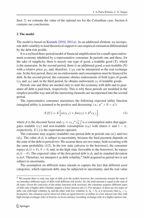
Sect. 5, we estimate the value of the optimal tax for the Colombian case. Section 6contains our conclusions.

2 The model

The model is based on Korinek (2010, 2011a). As an additional element, we incorpo-rate debt volatility to lend theoretical support to our empirical estimation differentiatedby the debt-risk profile.

It is a stylized three-period model of financial amplification for a small open endow-ment economy inhabited by a representative consumer. In periods one and three, forthe sake of simplicity, there is merely one type of good, a tradable good (T), whichis the numeraire. In the second period, there is an additional good, a non-tradable (N)with a relative price p2, and, therefore, 1/p2 can be interpreted as the real exchangerate. In the first period, there are no endowments and consumption must be financed bydebt. In the second period, the consumer obtains endowments of both types of goods(yT and yN) and, in the third period, he obtains endowment yT of tradable goods.

Periods one and three are needed only to start the economy with debt and to guar-antee all debt is paid back, respectively. This is why these periods are modeled in thesimplest possible way and all the interesting elements are incorporated into the secondperiod.

The representative consumer maximizes the following expected utility function(marginal utility is assumed to be positive and decreasing: i.e., u′′ < 0 < u′):

E [U ] = E[u(cT,1) + βu(c2) + β2cT,3

], (1)

where β is the discount factor and c2 = cT,2σ c1−σ

N,2 is a consumption index that aggre-gates tradable (cT) and non-tradable consumption (cN) with shares σ and 1 − σ ,respectively. E [.] is the expectations operator.

The consumer may acquire (tradable) one-period debt in periods one (d1) and two(d2). The value of d1 is subject to uncertainty, because the final payment depends onthe state of the debt in period two. We assume there are two states, both occurring withthe same probability (1/2). In the low state (adverse to the borrower), the consumerrepays d1(1 + θ), θ > 0, and, in the high state (favorable to the borrower), he repaysd1(1 − θ). The expected value of the first-period debt is d1 and its standard deviationis d1θ . Therefore, we interpret θ as debt volatility.6 Debt acquired in period two is notsubject to uncertainty.

The assumption on different states intends to capture the fact that different assetcategories, which represent debt, may be subjected to uncertainty, and the real value

6 We assume there is only one type of debt d1in the model; however, the conclusions remain the same ifwe introduce different types of debt (with different risk levels). So, the total amount is equal to the sum ofall types. Given the concavity of the utility function (risk aversion), the consumer acquires different typesof debt only if higher debt volatility implies a lower interest rate (r). For instance, if there are two types ofdebt, one with high volatility θh and the other with low volatility θl, θh > θl, it is necessary that rh < rl.In practice, this situation can be observed when an agent borrows in dollars at a low interest rate (but withhigh foreign exchange risk) or borrows in local currency (avoiding exchange risk) at a higher interest rate.

123


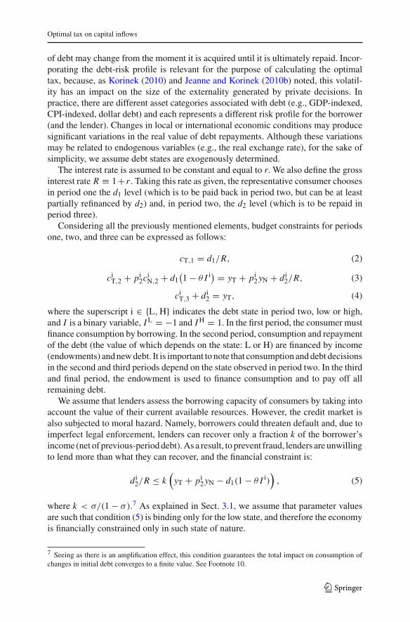
of debt may change from the moment it is acquired until it is ultimately repaid. Incor-porating the debt-risk profile is relevant for the purpose of calculating the optimaltax, because, as Korinek (2010) and Jeanne and Korinek (2010b) noted, this volatil-ity has an impact on the size of the externality generated by private decisions. Inpractice, there are different asset categories associated with debt (e.g., GDP-indexed,CPI-indexed, dollar debt) and each represents a different risk profile for the borrower(and the lender). Changes in local or international economic conditions may producesignificant variations in the real value of debt repayments. Although these variationsmay be related to endogenous variables (e.g., the real exchange rate), for the sake ofsimplicity, we assume debt states are exogenously determined.

The interest rate is assumed to be constant and equal to r. We also define the grossinterest rate R ≡ 1+r . Taking this rate as given, the representative consumer choosesin period one the d1 level (which is to be paid back in period two, but can be at leastpartially refinanced by d2) and, in period two, the d2 level (which is to be repaid inperiod three).

Considering all the previously mentioned elements, budget constraints for periodsone, two, and three can be expressed as follows:

cT,1 = d1/R, (2)

ciT,2 + pi

2ciN,2 + d1

(1 − θ I i) = yT + pi

2 yN + d i2/R, (3)

ciT,3 + d i

2 = yT, (4)

where the superscript i ∈ {L, H} indicates the debt state in period two, low or high,and I is a binary variable, I L = −1 and I H = 1. In the first period, the consumer mustfinance consumption by borrowing. In the second period, consumption and repaymentof the debt (the value of which depends on the state: L or H) are financed by income(endowments) and new debt. It is important to note that consumption and debt decisionsin the second and third periods depend on the state observed in period two. In the thirdand final period, the endowment is used to finance consumption and to pay off allremaining debt.

We assume that lenders assess the borrowing capacity of consumers by taking intoaccount the value of their current available resources. However, the credit market isalso subjected to moral hazard. Namely, borrowers could threaten default and, due toimperfect legal enforcement, lenders can recover only a fraction k of the borrower’sincome (net of previous-period debt). As a result, to prevent fraud, lenders are unwillingto lend more than what they can recover, and the financial constraint is:

d i2/R ≤ k

(yT + pi

2 yN − d1(1 − θ I i))

, (5)

where k < σ/(1 − σ).7 As explained in Sect. 3.1, we assume that parameter valuesare such that condition (5) is binding only for the low state, and therefore the economyis financially constrained only in such state of nature.

7 Seeing as there is an amplification effect, this condition guarantees the total impact on consumption ofchanges in initial debt converges to a finite value. See Footnote 10.

123


The foregoing equation introduces a crucial feature of the model; that is, whenevaluating the debt capacity of potential borrowers, lenders take into account not onlythe borrowers’ assets (endowments), but also the borrowers’ previously acquired debt.By including liabilities (previously acquired but still in force) in the financial constraintwe are incorporating a fact that has been neglected by traditional constraints: the lenderwill not regard as equal two people with the same income but with different levelsof initial debt. The maximum amount of credit that the borrower with higher initialdebt can obtain should be lower than that of the other one because the former alreadyowes a higher proportion of his income. In other words we are taking into accountthat previous overborrowing reduces debt capacity. Since borrowers are aware of thisfact, they have additional incentives to limit their debt and the externality that arisesduring crises is smaller than the one calculated without such effect.

Furthermore, Eq. (5) introduces both the amplification effects considered by thetraditional constraint8 and the fact that higher volatility (θ ) may have a negative impacton the financial constraint. It also incorporates the effect of the real exchange rate onborrowing capacity and, as Korinek (2010) mentioned, it captures the common notionthat depreciations (↓ p2) may contribute to the contraction of emerging economies.

3 Equilibrium

The model is solved through backward induction; that is, first for periods two andthree, taking the initial debt level d1as given. In making consumption decisions forperiods two and three, the representative consumer already has seen the state of periodtwo. Therefore, this part of the solution implies no uncertainty. We obtain solutions forboth the decentralized case and the one where a CP decides the consumption level. Bycomparing these two solutions, we can show private agents undervalue liquidity rela-tive to the CP when the economy is financially constrained. Given this result and thesolution for period one (where there is uncertainty about the state of period two), thedecentralized solution is shown to imply overborrowing. In other words, a CP wouldacquire a lower debt level in period one. This last result rationalizes the introduction ofpolicy actions that may reduce the size of the externality generated by private agents’decisions.

As a benchmark case, consider an economy without the financial constraint (5)such that the consumer is only constrained by his income flow (i.e., the inter-temporalbudget constraint). Since the valuation of liquidity of private agents and that of theCP differs only when the economy is financially constrained, without such constraintthere would be no externality and hence no reason for a positive tax. This is formallyshown in Sect. 4.

3.1 Decentralized equilibrium

By substituting (4) into (1), then maximizing subject to constraints (3) and (5),and considering the market-clearing conditions (ci

N,2 = yN, for non-tradables and

8 This has become an essential feature of a now common theoretical framework built on a positive descrip-tion of financial crises proposed by Mendoza (2002, 2005).

123


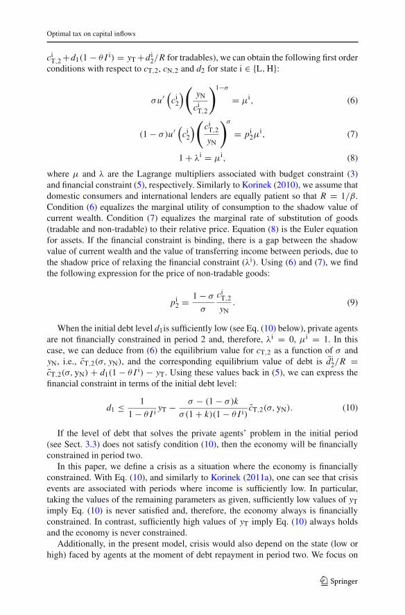
ciT,2 +d1(1 − θ I i) = yT +d i

2/R for tradables), we can obtain the following first orderconditions with respect to cT,2, cN,2 and d2 for state i ∈ {L, H}:

σu′ (ci2

) (yN

ciT,2

)1−σ

= μi, (6)

(1 − σ)u′ (ci2

) (ci

T,2

yN

)σ

= pi2μ

i, (7)

1 + λi = μi, (8)

where μ and λ are the Lagrange multipliers associated with budget constraint (3)and financial constraint (5), respectively. Similarly to Korinek (2010), we assume thatdomestic consumers and international lenders are equally patient so that R = 1/β.Condition (6) equalizes the marginal utility of consumption to the shadow value ofcurrent wealth. Condition (7) equalizes the marginal rate of substitution of goods(tradable and non-tradable) to their relative price. Equation (8) is the Euler equationfor assets. If the financial constraint is binding, there is a gap between the shadowvalue of current wealth and the value of transferring income between periods, due tothe shadow price of relaxing the financial constraint (λi). Using (6) and (7), we findthe following expression for the price of non-tradable goods:

pi2 = 1 − σ

σ

ciT,2

yN. (9)

When the initial debt level d1is sufficiently low (see Eq. (10) below), private agentsare not financially constrained in period 2 and, therefore, λi = 0, μi = 1. In thiscase, we can deduce from (6) the equilibrium value for cT,2 as a function of σ andyN, i.e., c̄T,2(σ, yN), and the corresponding equilibrium value of debt is d̄ i

2/R =c̄T,2(σ, yN) + d1(1 − θ I i) − yT. Using these values back in (5), we can express thefinancial constraint in terms of the initial debt level:

d1 ≤ 1

1 − θ I i yT − σ − (1 − σ)k

σ(1 + k)(1 − θ I i)c̄T,2(σ, yN). (10)

If the level of debt that solves the private agents’ problem in the initial period(see Sect. 3.3) does not satisfy condition (10), then the economy will be financiallyconstrained in period two.

In this paper, we define a crisis as a situation where the economy is financiallyconstrained. With Eq. (10), and similarly to Korinek (2011a), one can see that crisisevents are associated with periods where income is sufficiently low. In particular,taking the values of the remaining parameters as given, sufficiently low values of yTimply Eq. (10) is never satisfied and, therefore, the economy always is financiallyconstrained. In contrast, sufficiently high values of yT imply Eq. (10) always holdsand the economy is never constrained.

Additionally, in the present model, crisis would also depend on the state (low orhigh) faced by agents at the moment of debt repayment in period two. We focus on

123


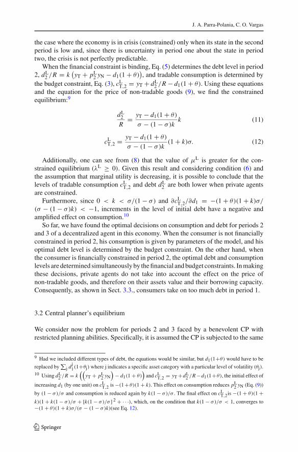
the case where the economy is in crisis (constrained) only when its state in the secondperiod is low and, since there is uncertainty in period one about the state in periodtwo, the crisis is not perfectly predictable.

When the financial constraint is binding, Eq. (5) determines the debt level in period2, dL

2 /R = k(yT + pL

2 yN − d1(1 + θ)), and tradable consumption is determined by

the budget constraint, Eq. (3), cLT,2 = yT + dL

2 /R − d1(1 + θ). Using these equationsand the equation for the price of non-tradable goods (9), we find the constrainedequilibrium:9

dL2

R= yT − d1(1 + θ)

σ − (1 − σ)kk (11)

cLT,2 = yT − d1(1 + θ)

σ − (1 − σ)k(1 + k)σ. (12)

Additionally, one can see from (8) that the value of μL is greater for the con-strained equilibrium (λL ≥ 0). Given this result and considering condition (6) andthe assumption that marginal utility is decreasing, it is possible to conclude that thelevels of tradable consumption cL

T,2 and debt dL2 are both lower when private agents

are constrained.Furthermore, since 0 < k < σ/(1 − σ) and ∂cL

T,2/∂d1 = −(1 + θ)(1 + k)σ/

(σ − (1 − σ)k) < −1, increments in the level of initial debt have a negative andamplified effect on consumption.10

So far, we have found the optimal decisions on consumption and debt for periods 2and 3 of a decentralized agent in this economy. When the consumer is not financiallyconstrained in period 2, his consumption is given by parameters of the model, and hisoptimal debt level is determined by the budget constraint. On the other hand, whenthe consumer is financially constrained in period 2, the optimal debt and consumptionlevels are determined simultaneously by the financial and budget constraints. In makingthese decisions, private agents do not take into account the effect on the price ofnon-tradable goods, and therefore on their assets value and their borrowing capacity.Consequently, as shown in Sect. 3.3., consumers take on too much debt in period 1.

3.2 Central planner’s equilibrium

We consider now the problem for periods 2 and 3 faced by a benevolent CP withrestricted planning abilities. Specifically, it is assumed the CP is subjected to the same

9 Had we included different types of debt, the equations would be similar, but d1(1+θ) would have to be

replaced by∑

j dj1(1+θj) where j indicates a specific asset category with a particular level of volatility (θj).

10 Using dL2 /R = k

((yT + pL

2 yN

)− d1(1 + θ)

)and cL

T,2 = yT +dL2 /R −d1(1+θ), the initial effect of

increasing d1 (by one unit) on cLT,2 is −(1 + θ)(1 + k). This effect on consumption reduces pL

2 yN (Eq. (9))

by (1 − σ)/σ and consumption is reduced again by k(1 − σ)/σ . The final effect on cLT,2is −(1 + θ)(1 +

k)(1 + k(1 − σ)/σ + [k(1 − σ)/σ ] 2 + · · ·), which, on the condition that k(1 − σ)/σ < 1, converges to−(1 + θ)(1 + k)σ/(σ − (1 − σ)k)(see Eq. 12).

123


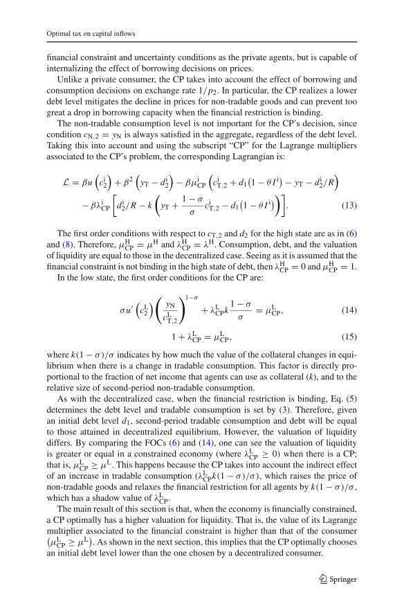
financial constraint and uncertainty conditions as the private agents, but is capable ofinternalizing the effect of borrowing decisions on prices.

Unlike a private consumer, the CP takes into account the effect of borrowing andconsumption decisions on exchange rate 1/p2. In particular, the CP realizes a lowerdebt level mitigates the decline in prices for non-tradable goods and can prevent toogreat a drop in borrowing capacity when the financial restriction is binding.

The non-tradable consumption level is not important for the CP’s decision, sincecondition cN,2 = yN is always satisfied in the aggregate, regardless of the debt level.Taking this into account and using the subscript “CP” for the Lagrange multipliersassociated to the CP’s problem, the corresponding Lagrangian is:

L = βu(

ci2

)+ β2

(yT − d i

2

)− βμi

CP

(ci

T,2 + d1(1 − θ I i) − yT − d i

2/R)

−βλiCP

[d i

2/R − k

(yT + 1 − σ

σci

T,2 − d1(1 − θ I i)

)]. (13)

The first order conditions with respect to cT,2 and d2 for the high state are as in (6)and (8). Therefore, μH

CP = μH and λHCP = λH. Consumption, debt, and the valuation

of liquidity are equal to those in the decentralized case. Seeing as it is assumed that thefinancial constraint is not binding in the high state of debt, then λH

CP = 0 and μHCP = 1.

In the low state, the first order conditions for the CP are:

σu′ (cL2

) (yN

cLT,2

)1−σ

+ λLCPk

1 − σ

σ= μL

CP, (14)

1 + λLCP = μL

CP, (15)

where k(1 − σ)/σ indicates by how much the value of the collateral changes in equi-librium when there is a change in tradable consumption. This factor is directly pro-portional to the fraction of net income that agents can use as collateral (k), and to therelative size of second-period non-tradable consumption.

As with the decentralized case, when the financial restriction is binding, Eq. (5)determines the debt level and tradable consumption is set by (3). Therefore, givenan initial debt level d1, second-period tradable consumption and debt will be equalto those attained in decentralized equilibrium. However, the valuation of liquiditydiffers. By comparing the FOCs (6) and (14), one can see the valuation of liquidityis greater or equal in a constrained economy (where λL

CP ≥ 0) when there is a CP;that is, μL

CP ≥ μL. This happens because the CP takes into account the indirect effectof an increase in tradable consumption (λL

CPk(1 − σ)/σ), which raises the price ofnon-tradable goods and relaxes the financial restriction for all agents by k(1 − σ)/σ ,which has a shadow value of λL

CP.The main result of this section is that, when the economy is financially constrained,

a CP optimally has a higher valuation for liquidity. That is, the value of its Lagrangemultiplier associated to the financial constraint is higher than that of the consumer(μL

CP ≥ μL). As shown in the next section, this implies that the CP optimally chooses

an initial debt level lower than the one chosen by a decentralized consumer.

123


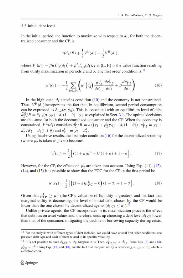
3.3 Initial debt level

In the initial period, the function to maximize with respect to d1, for both the decen-tralized consumer and the CP, is:

u(d1/R) + 1

2V L(d1) + 1

2V H(d1),

where V i(d1) = βu(ci

2(d1)) + β2ci

T,3(d1), i ∈ {L, H} is the value function resultingfrom utility maximization in periods 2 and 3. The first order condition is:11

u′(c1) = −1

2

∑i=L,H

(u′ (ci

2

) dci2

dciT,2

dciT,2

dd1+ β

dciT,3

dd1

). (16)

In the high state, d1 satisfies condition (10) and the economy is not constrained.Thus, V H(d1)incorporates the fact that, in equilibrium, second period consumptioncan be expressed as c̄T,2(σ, yN). This is associated with an equilibrium level of debtd̄H

2 /R = c̄T,2(σ, yN)+d1(1 − θ)−yT, as explained in Sect. 3.1. The optimal decisionsare the same for both the decentralized consumer and the CP. When the economy isconstrained, V L(d1) considers dL

2 /R = k((

yT + pL2 yN

) − d1(1 + θ)), cL

T,2 = yT +dL

2 /R2 − d1(1 + θ) and cLT,3 = yT − dL

2 .Using the above results, the first order condition (16) for the decentralized economy

(where pi2 is taken as given) becomes:

u′(c1) = 1

2

[((1 + k)μL − k)(1 + θ) + 1 − θ

]. (17)

However, for the CP, the effects on pi2 are taken into account. Using Eqs. (11), (12),

(14), and (15) it is possible to show that the FOC for the CP in the first period is:

u′(c1) = 1

2

[((1 + k)μL

PC − k)

(1 + θ) + 1 − θ]. (18)

Given that μLCP ≥ μL (the CP’s valuation of liquidity is greater), and the fact that

marginal utility is decreasing, the level of initial debt chosen by the CP would belower than the one chosen by decentralized agents (d1,CP ≤ d1).12

Unlike private agents, the CP incorporates in its maximization process the effectthat debt has on asset values and, therefore, ends up choosing a debt level d1,CP lowerthan that of the consumer, mitigating the decline of borrowing capacity during crisis.

11 For the analysis with different types of debt included, we would have several first order conditions, oneper each debt type and each of them related to its specific volatility.12 It is not possible to have d1,CP > d1. Suppose it is. Then, cL

T,2,CP < cLT,2. From Eqs. (6) and (14),

μLCP > μL. Using Eqs. (17) and (18), and the fact that marginal utility is decreasing, d1,CP < d1, which is

a contradiction.

123


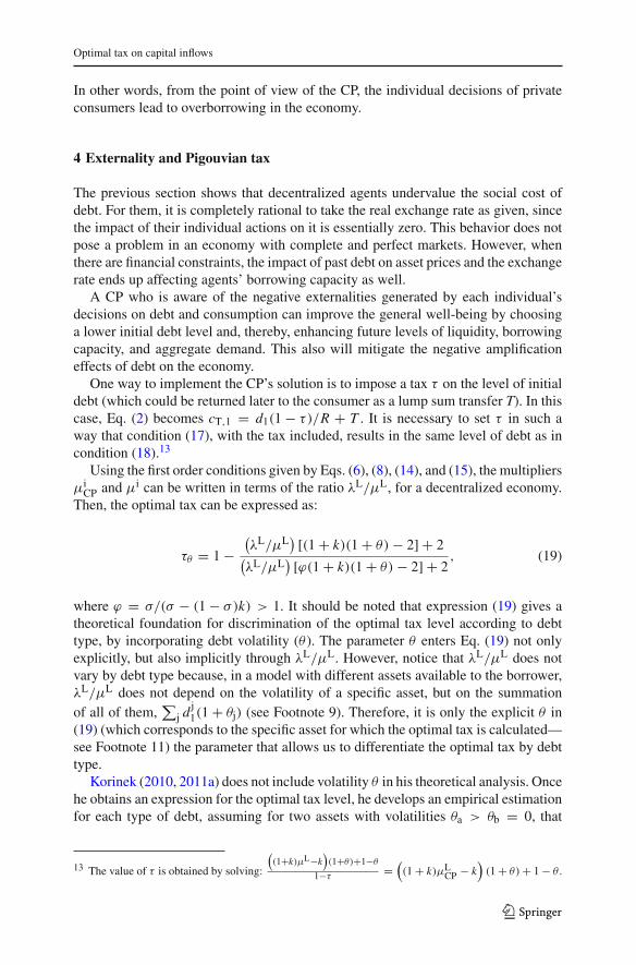
In other words, from the point of view of the CP, the individual decisions of privateconsumers lead to overborrowing in the economy.

4 Externality and Pigouvian tax

The previous section shows that decentralized agents undervalue the social cost ofdebt. For them, it is completely rational to take the real exchange rate as given, sincethe impact of their individual actions on it is essentially zero. This behavior does notpose a problem in an economy with complete and perfect markets. However, whenthere are financial constraints, the impact of past debt on asset prices and the exchangerate ends up affecting agents’ borrowing capacity as well.

A CP who is aware of the negative externalities generated by each individual’sdecisions on debt and consumption can improve the general well-being by choosinga lower initial debt level and, thereby, enhancing future levels of liquidity, borrowingcapacity, and aggregate demand. This also will mitigate the negative amplificationeffects of debt on the economy.

One way to implement the CP’s solution is to impose a tax τ on the level of initialdebt (which could be returned later to the consumer as a lump sum transfer T). In thiscase, Eq. (2) becomes cT,1 = d1(1 − τ)/R + T . It is necessary to set τ in such away that condition (17), with the tax included, results in the same level of debt as incondition (18).13

Using the first order conditions given by Eqs. (6), (8), (14), and (15), the multipliersμi

CP and μi can be written in terms of the ratio λL/μL, for a decentralized economy.Then, the optimal tax can be expressed as:

τθ = 1 −(λL/μL

)[(1 + k)(1 + θ) − 2] + 2(

λL/μL)

[ϕ(1 + k)(1 + θ) − 2] + 2, (19)

where ϕ = σ/(σ − (1 − σ)k) > 1. It should be noted that expression (19) gives atheoretical foundation for discrimination of the optimal tax level according to debttype, by incorporating debt volatility (θ ). The parameter θ enters Eq. (19) not onlyexplicitly, but also implicitly through λL/μL. However, notice that λL/μL does notvary by debt type because, in a model with different assets available to the borrower,λL/μL does not depend on the volatility of a specific asset, but on the summationof all of them,

∑j d j

1(1 + θj) (see Footnote 9). Therefore, it is only the explicit θ in(19) (which corresponds to the specific asset for which the optimal tax is calculated—see Footnote 11) the parameter that allows us to differentiate the optimal tax by debttype.

Korinek (2010, 2011a) does not include volatility θ in his theoretical analysis. Oncehe obtains an expression for the optimal tax level, he develops an empirical estimationfor each type of debt, assuming for two assets with volatilities θa > θb = 0, that

13 The value of τ is obtained by solving:

((1+k)μL−k

)(1+θ)+1−θ

1−τ=

((1 + k)μL

CP − k)

(1 + θ) + 1 − θ .

123


τθa = (1 + θa)τθb . In contrast, the analysis in this paper shows the ratio τθa/τθb doesnot necessarily increase one-to-one with the value of (1 + θa), as explained in the nextsection.

Notice that if there were no market imperfections (no financial constraint), we wouldhave μL

CP = μL for the low state of nature (as in the case for the high state, because thefinancial constraint is non-binding). In such case, Eqs., (17) and (18) imply the samelevel of initial debt for both the decentralized case and the CP case. Consequently,there would be neither externality nor a positive Pigouvian tax. This can be formallyseen in Eq. (19) by assuming the financial constraint is non-binding (λL = 0). Underthis assumption, τθ = 0.

5 Empirical approximation

Pursuant to the sufficient statistics approach described by Chetty (2009), Eq. (19) hasbeen derived so that, on the one hand, θ is shown separately to calculate the tax byasset type. On the other hand, all the other structural parameters of the model remaingrouped in order to use the agents’ first order conditions.

The main idea behind this approach is to concentrate the calibration on those vari-ables relevant to the study (in this case, the optimal tax value), instead of tryingto identify all the relations that are part of the underlying structural model. In thisway, it is possible to reduce the number of components to be identified, while keep-ing the primitive parameters of the model grouped into elements directly related tothe first order conditions (e.g., elasticities or, as is the case in this paper, Lagrangemultipliers).

By not requiring the estimated variables to depend directly on specific parametersand, therefore, on the exact structure of the model, the theoretical results can be pre-sented in a simple and tractable way.14 The calibration results can also be valid formore general forms of the same model or for models with similar structures. Further-more, by reducing the number of elements to be identified, the sufficient statisticsapproach allows for minimum data availability requirements.15

Naturally, the aforementioned advantages definitely come at a cost. The main draw-back of not expressing the tax in terms of the structural parameters of the model is thatit becomes impossible to perform an appropriate sensitivity or counterfactual analy-sis of the results.16 To compensate for this disadvantage and to have a standard ofhow reasonable or robust the estimation is, the intermediate results or final values are

14 In Eq. (19), the expression for λL/μL in terms of the primitive parameters is in closed form only forvery particular cases (e.g., logarithmic utility functions).15 For example, in this paper, calculating the optimal tax by estimating the primitive parameters wouldnecessitate, among other things, estimating the value of interest rates and the volatility of every single assetrelevant to the entry of capital flows into Colombia. This data requirement comes from the fact that λL/μL

incorporates information on cLT,2 and dL

2 , and estimating them calls for information on the aforementionedassets (see Footnote 9).16 For example, it is not appropriate to analyze how the optimal tax value changes in response to changesin k, using Eq. (19), if the fact that k affects the value of λL/μLis not taken into account.

123


compared, wherever possible, to those obtained in other recent studies related to thispaper.

The reference point to calculate the value of the optimal tax is the informationtaken from the 1998–1999 period, which is considered the most recent period offinancial crisis in Colombia [see, e.g., Villar et al. (2005); Gómez and Kiefer (2006)]characterized by economic recession, a collapse in the exchange rate band, and a strongcredit contraction.

Based on Eq. (19), estimating the tax value requires calculating five components17:

• The tightness of constraints, λL/μL. This factor measures the marginal increasein utility that comes from relaxing the financial constraint, normalized by themarginal valuation of liquidity. Similarly to Korinek (2010) and assuming a util-ity function with constant relative risk aversion (CRRA), the change in mar-ginal utility is approximated using the change in real consumption during thecrisis. Taking γ as the risk aversion coefficient, the estimation for Colombiais18:

λL

μL ≈ −γ · Ccrisis + γ (1 + γ )

2(Ccrisis)2

≈ −(

1

0.42· −4.1 %

)+ 4.02 · (−4.1 %)2 ≈ 9.1 %,

using the value estimated by Prada and Rojas (2010) for the inter-temporal elas-ticity of substitution (1/γ ) for Colombia.

• The proportion of non-tradable consumption, 1 − σ , is estimated as an average ofthe ratio of real production of non-tradable goods to real total consumption for theperiod 1996Q1-2011Q3, 1 − σ ≈ 71 %.19

• Proportion k measures the borrowing capacity of the economy. This value, as sug-gested by the model, will be observable only during a crisis20 (when the financial

17 The Korinek model (2011b) requires the estimation of 9 parameters, 10 in that of Mendoza (2010), 12 inthat of Bianchi and Mendoza (2011), and 15 in that of Bianchi (2011). None of these models differentiatesthe value of the tax by the type of capital flows. However, some of them stochastically model income flows(e.g., 8 out of the 15 parameters estimated by Bianchi (2011) are required to that end).18 The calibration of this ratio is based on a second order Taylor approximation of the Euler equation inKorinek (2010), which is similar to the one in this paper (Eq. (8)), but more general because it correspondsto a model with infinite periods. In Korinek (2010), the equation is λ/μ = 1−u′(ct+1)/u′(ct ). The secondorder Taylor approximation on ct+1 = ct results in λ/μ ≈ −γ (ct+1/ct ) + γ (1 + γ )(ct+1/ct )

2/2.Korinek (2010) resorts to a first order approximation. However, in the present paper, the second order effectsare significant for the estimate at the second-decimal level.19 The value is highly stable throughout the period, reaching a minimum of 69 % and a maximum of 73 %.It also is similar to the one calibrated by Bianchi (2011) for Argentina (69 %).20 For its numerical examples, Korinek (2010) takes the maximum value of debt over GDP estimated byReinhart et al. (2003) at 50 %. However, maximum values could be reached at times when the economyis not in crisis (e.g., in times of high liquidity and international financial boom). Therefore, because theeconomy is not financially constrained, those values would not be a good approximation of k.

123


constraint is satisfied with equality). To estimate it, the ratio between foreign debtin constant pesos and real GDP for 1999 is used.21 In this case22:

k ≈ Debt99

GDP99≈ 33.6 %

• The volatility factor, by debt or asset type, θ . In the model, θ represents both thepercentage change and the volatility in the real value of debt (net of interest) withrespect to its original value. To illustrate the effect of that volatility on the optimaltax, this paper assumes two asset types. On the one hand, the estimation is madefor a credit instrument (called type b) contracted in CPI-indexed pesos, so its realvalue does not change. In this case, θb = 0. On the other, an estimation is madefor a credit instrument (type a) contracted in dollars; thus, its real value increaseswith devaluation and decreases with inflation such that the percentage changeof debt is equal to (1 + Dev)/(1 + π) − 1 = (Dev − π)/(1 + π), where Devis devaluation and π is inflation. With data for 1996–2011, the average absolutevalue of (Dev − π)/(1 + π) is θa ≈ 9.5 %. It should be noted that estimating θ

as an average for the entire period is probably the approach most consistent withthe model, where it is assumed debt value variations do not depend on a crisisoccurring (but the latter does depend on the former). However, as an alternativeinterpretation and additional exercise, a higher value of θ from the crisis is used.For the September 1998–August 1999 period, the value of (Dev − π)/(1 + π) isθa′ ≈ 24.1 %.

• With the figures specified above, sufficient information is available to calculate theoptimal tax rate that would be imposed on the debt level the year prior to a crisis.However, as it is difficult to anticipate a crisis and, even if that were possible, thetax would be too high if imposed on a specific period (as a percentage of currenttotal debt), it seems convenient to spread it out among all the periods. To that end,the externality value is multiplied by the probability of a crisis, which is assumedto be 5 %, the same as in Korinek (2010) for Indonesia, similar to the value used byBianchi (2011) for Argentina (5.5 %), and higher than the one assumed by Bianchiand Mendoza (2011) for the United States (3 %).

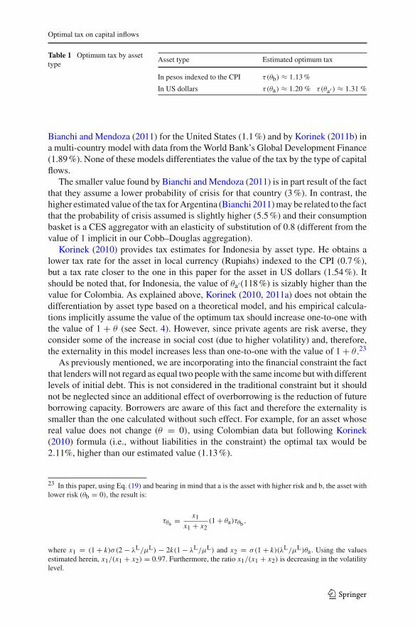
Using Eq. (19) and the aforementioned values, the results are listed in Table 1.These findings suggest the optimum tax value for Colombia, according to the type

of asset volatility, would lie between 1.1 and 1.3 %. This is higher than the value foundby Jeanne and Korinek (2010b) for the United States (0.56 %), lower than the one deter-mined by Bianchi (2011) for Argentina (3.6 %), and closer to the estimates made by

21 In solving Eq. (5) for k (when the restriction is binding), the result suggests this parameter should beestimated as the ratio of total debt to net income. However, the simplifications in the model do not makethat approach necessarily the most precise one. For example, in the model, debt is paid back in one period;however, in reality, it could be amortized within different time frames. For this reason, a small modificationis made, and the borrowing capacity of a constrained economy is measured in a more standard way similarto what is found in other documents (e.g., Korinek (2010)), using the debt level as a proportion of GDP.22 The obtained value is consistent with those estimated by Bianchi (2011) (32 %) and by Bianchi andMendoza (2011) (36 %), who calibrated the value of k so their models would reproduce the likelihood of acrisis in Argentina and the United States, respectively. In a similar exercise, Mendoza (2010) estimates avalue of 20 % for Mexico.

123


Table 1 Optimum tax by assettype

Asset type Estimated optimum tax

In pesos indexed to the CPI τ(θb) ≈ 1.13 %

In US dollars τ(θa) ≈ 1.20 % τ(θa′ ) ≈ 1.31 %

Bianchi and Mendoza (2011) for the United States (1.1 %) and by Korinek (2011b) ina multi-country model with data from the World Bank’s Global Development Finance(1.89 %). None of these models differentiates the value of the tax by the type of capitalflows.

The smaller value found by Bianchi and Mendoza (2011) is in part result of the factthat they assume a lower probability of crisis for that country (3 %). In contrast, thehigher estimated value of the tax for Argentina (Bianchi 2011) may be related to the factthat the probability of crisis assumed is slightly higher (5.5 %) and their consumptionbasket is a CES aggregator with an elasticity of substitution of 0.8 (different from thevalue of 1 implicit in our Cobb–Douglas aggregation).

Korinek (2010) provides tax estimates for Indonesia by asset type. He obtains alower tax rate for the asset in local currency (Rupiahs) indexed to the CPI (0.7 %),but a tax rate closer to the one in this paper for the asset in US dollars (1.54 %). Itshould be noted that, for Indonesia, the value of θa′(118 %) is sizably higher than thevalue for Colombia. As explained above, Korinek (2010, 2011a) does not obtain thedifferentiation by asset type based on a theoretical model, and his empirical calcula-tions implicitly assume the value of the optimum tax should increase one-to-one withthe value of 1 + θ (see Sect. 4). However, since private agents are risk averse, theyconsider some of the increase in social cost (due to higher volatility) and, therefore,the externality in this model increases less than one-to-one with the value of 1 + θ .23

As previously mentioned, we are incorporating into the financial constraint the factthat lenders will not regard as equal two people with the same income but with differentlevels of initial debt. This is not considered in the traditional constraint but it shouldnot be neglected since an additional effect of overborrowing is the reduction of futureborrowing capacity. Borrowers are aware of this fact and therefore the externality issmaller than the one calculated without such effect. For example, for an asset whosereal value does not change (θ = 0), using Colombian data but following Korinek(2010) formula (i.e., without liabilities in the constraint) the optimal tax would be2.11%, higher than our estimated value (1.13 %).

23 In this paper, using Eq. (19) and bearing in mind that a is the asset with higher risk and b, the asset withlower risk (θb = 0), the result is:

τθa = x1

x1 + x2(1 + θa)τθb ,

where x1 = (1 + k)σ (2 − λL/μL) − 2k(1 − λL/μL) and x2 = σ(1 + k)(λL/μL)θa. Using the valuesestimated herein, x1/(x1 + x2) = 0.97. Furthermore, the ratio x1/(x1 + x2) is decreasing in the volatilitylevel.

123


6 Conclusions

This paper follows recent economic literature that suggests it is convenient to takeprudential policy measures to reduce financial vulnerability in times of crisis. Theexpediency of these measures lies with the existence of international financial marketimperfections (e.g., economies face credit constraints) and the fact that private agentsdo not internalize the social costs of their consumption/debt plans, which have aneffect on prices and, ultimately, on the borrowing capacity of the economy.

Because decentralized agents (rationally) underestimate the impact of their deci-sions, there is a negative externality that amplifies social costs in times of crisis. Thisexternality can be corrected by imposing a Pigouvian tax on capital inflows, as sug-gested in this paper.

The model is similar to others described in related literature and, as a contribution, itincludes pending liabilities in the financial constraint and the fact that the real value ofdebt may be subjected to uncertainty (due to factors like inflation or devaluation). In thisway we provide a theoretical foundation for estimating the optimum tax differentiatedby debt volatility and incorporate a fact that has been neglected by traditional financialconstraints: that such liabilities reduce debt capacity. As a result, borrowers haveadditional incentives to limit their debt and thus the optimal tax is smaller than theone calculated without regarding this fact.

Using Colombian data for the 1996–2011 period (and considering 1998–1999 asa time of financial crisis), an empirical exercise is performed to calculate the valueof the optimum tax. The results suggest the tax on capital inflows would be around1.2 %, which is similar in magnitude to the values obtained in related literature.

Considering differences in volatility, the estimation was made for two types of debt:CPI-indexed Colombia peso debt and US dollar debt. The results suggest the optimumtax would be 1.1 % in the first case and within the 1.2–1.3 % range for the second typeof debt. The difference between the two cases is small, since the difference betweendevaluation and inflation in Colombia in recent decades has not been large.

Our estimation is based on simplifying assumptions that make the calculation sus-ceptible to improvement in different aspects and could serve as a motivation for futureresearch. As to extensions of this model, the productive sectors and the accumulationof capital could be modeled to endogenize the agent’s income flows, as well as thedifferent forms of financing domestic production. As suggested by Korinek (2010),foreign direct investment is a form of finance that may not create negative external-ities (and therefore not subjected to a tax) as long as it is unlikely to entail capitaloutflows during crisis and, to the contrary, may contribute to increase future output.It is important for policymakers not to neglect this possibility because it might resultin too high a tax and reduce capital inflows for productive means. This is a significantremark that needs theoretical support.

Another aspect that we left for future research is the introduction of a more gen-eral distribution of the states of nature which allows for the endogenization of theprobability of crisis.

Acknowledgments The authors wish to thank the editor, Eckhard Janeba, and two anonymous referees forhelpful comments. We also thank J. Bejarano, J. E. Gomez, J. Ojeda, H. Rincon, H. Vargas and A. Velasco for

123


their valuable suggestions; A. Korinek for clarifications on the empirical analysis of his document (Korinek2010). The opinions expressed herein are solely the responsibility of the authors and do not necessarilyreflect those of the Central Bank of Colombia or its Board of Directors.

References

Aghion, P., Bacchetta, P., & Banerjee, A. (2004). Financial development and the instability of openeconomies. Journal of Monetary Economics, 51, 1077–1106.

Bernanke, B., & Gertler, M. (1989). Agency costs, net worth and business fluctuations. American EconomicReview, 79, 14–31.

Bianchi, J. (2011). Overborrowing and systemic externalities in the business cycle. American EconomicReview, 101(7), 3400–3426.

Bianchi, J., & Mendoza, E. (2011). Overborrowing, financial crises and ‘macro-prudential’ policy. WorkingPaper No. 11–24, International Monetary Fund.

Caballero, R. J., & Krishnamurthy, A. (2001). International and domestic collateral constraints in a modelof emerging market crises. Journal of Monetary Economics, 48(3), 513–548.

Caballero, R. J., & Krishnamurthy, A. (2003). Excessive dollar debt: Financial development and underin-surance. Journal of Finance, 58(2), 867–894.

Caballero, R. J., & Krishnamurthy, A. (2004). Smoothing sudden stops. Journal of Economic Theory,119(1), 104–127.

Chetty, R. (2009). Sufficient statistics for welfare analysis: A bridge between structural and reduced-formmethods. Annual Review of Economics, 1(1), 451–487.

Geanakoplos, J., & Polemarchakis, H. (1986). Existence, regularity, and constrained suboptimality of com-petitive allocations when markets are incomplete. In W. P. Heller, R. M. Ross, & D. A. Starrett (Eds.),Uncertainty, information and communication: Essays in honor of Kenneth Arrow. Cambridge: Cam-bridge University Press.

Gómez J., & Kiefer, N. (2006). Bank failure: Evidence from the Colombian financial crisis. Working PaperNo. 06–12, Cornell University.

Greenwald, B. C., & Stiglitz, J. E. (1986). Externalities in economies with imperfect information andincomplete markets. The Quarterly Journal of Economics, 101(2), 229–264.

Jeanne, O., & Korinek, A. (2010a). Excessive volatility in capital flows: A Pigouvian taxation approach.American Economic Review: Papers and Proceedings, 100(2), 403–407.

Jeanne, O., & Korinek, A. (2010b). Managing credit booms and busts: A Pigouvian taxation approach.NBER Working Paper No. 16377.

Kiyotaki, N., & Moore, J. (1997). Credit cycles. Journal of Political Economy, 105, 211–248.Korinek, A. (2010). Regulating capital flows to emerging markets: An externality view. Mimeo, University

of Maryland.Korinek, A. (2011a). The new economics of prudential capital controls: A research agenda. IMF Economic

Review, 59(3), 523–561.Korinek, A. (2011b). Hot money and serial financial crises. IMF Economic Review, 59(59), 306–339.Krugman, P. (1979). A model of balance-of-payment crises. Journal of Money Credit and Banking, 11(3),

311–325.Mendoza, E. (2002). Credit, prices, and crashes: Business cycles with a sudden stop. In S. Edwards &

J. A. Frankel (Eds.), Preventing currency crises in emerging markets. Chicago, IL: University of ChicagoPress and National Bureau of Economic Research.

Mendoza, E. (2005). Real exchange rate volatility and the price of nontradable goods in economies proneto sudden stops. Economia, 6(1), 103–105.

Mendoza, E. (2010). Sudden stops, financial crises, and leverage. American Economic Review, 100, 1941–1966.

Obstfeld, M. (1994). The logic of currency crises. Cahiers Economiques et Monetaries, 43, 189–213.Prada, J., & Rojas, L. (2010). La Elasticidad de Frisch y la Transmisión de la Política Monetaria en Colombia.

In M. Jalil & L. Mahadeva (Eds.), Mecanismos de transmisión de la Política Monetaria en Colombia,chapter 13. Bogotá: Banco de la República and Universidad Externado de Colombia.

Reinhart, C., Rogoff, K., & Savastano, M. (2003). Debt intolerance. Brookings Papers on Economic Activity,Economic Studies Program, 34(1), 1–74.

123


Stein, J. (2012). Monetary policy as financial stability regulation. The Quarterly Journal of Economics,127, 57–95.

Villar, L., Salamanca, D., & Murcia, A. (2005). Crédito, represión financiera y flujos de capitales enColombia 1974–2003. Desarrollo y Sociedad, 55, 167–209.

123

Documents

Optimal tax on capital inflows discriminated by debt-risk profile