Optimal provision of implicit and explicit incentives in

asset management contracts�

Samy Osamu Abud Yoshima

EPGE-FGV/RJ - Advisor: Professor Luis Henrique B. Braido

July 13, 2005

Abstract

This paper investigates the importance of the �ow of funds as an implicit incentive

provided by investors to portfolio managers. We build a two-period binomial moral

hazard model to explain the main trade-o¤s in the relationship between �ow, fees

and performance. The main assumption is that e¤ort depends on the combination of

implicit and explicit incentives while the probability distribution function of returns

depends on e¤ort. In the case of full commitment, the investor�s relevant trade-o¤ is

to give up expected return in the second period vis-à-vis to induce e¤ort in the �rst

period. The more concerned the investor is with today�s payo¤, the more willing he

will be to give up expected return in the following periods.Whitout commitment, we

consider that the investor also learns some symmetric and imperfect information about

the ability of the manager to generate positive excess return. In this case, observed

returns reveal ability as well as e¤ort choices. We show that powerful implicit incentives

can explain the �ow-performance relationship and we provide a numerical solution in

Matlab that characterize these results.�This paper is part of my dissertation thesis to obtain the title of Master in Economics at EPGE-FGV/RJ.

I would like to thank Angelo Polydoro and Enrico Vasconcelos for computational and Matlab assistance;

Gustavo C. Branco and Guilherme Bragança from Mellon Brascan for the funds�data. Special thanks to

Amaury Fonseca Jr., Carlos Eugênio da Costa, Delano Franco, Fabiana D ´Atri, Fernando H. Barbosa,

Genaro Lins, Jaime Jesus Filho, Jair Koiller, Luis H. B. Braido, Marcelo Fernandez, and M. Cristina T.

Terra for guidance and fruitful discussions during the development of this project. Many other people have

contributed to the development of this project and I am thankful and indebted with them all.

1

Contents

1 Introduction 31.1 The literature . . . . . . . . . . . . . . . . . . . . . . . . . . . . . . . . . . . 4

1.2 Data and stylized facts . . . . . . . . . . . . . . . . . . . . . . . . . . . . . . 5

2 The model under full commitment 72.1 The timing of the model and the decision tree . . . . . . . . . . . . . . . . . 9

2.2 The portfolio manager problem: optimal choice of e¤ort . . . . . . . . . . . . 10

2.3 The investor problem: optimal provision of incentives . . . . . . . . . . . . . 12

2.4 Characterization of the optimal incentive contract . . . . . . . . . . . . . . . 14

2.4.1 Comparison with the case where �H = �L = 1 . . . . . . . . . . . . . 14

2.5 Numerical results . . . . . . . . . . . . . . . . . . . . . . . . . . . . . . . . . 19

3 The model with two types of portfolio managers 253.1 The portfolio manager problem: optimal choice of e¤ort . . . . . . . . . . . . 26

3.2 The investor problem: optimal provision of incentives . . . . . . . . . . . . . 27

3.3 Characterization of the optimal incentive contract . . . . . . . . . . . . . . . 28

3.4 Numerical results . . . . . . . . . . . . . . . . . . . . . . . . . . . . . . . . . 29

4 Conclusions 31

5 Appendix 345.1 CPO�s and equations of model in Section 2 . . . . . . . . . . . . . . . . . . . 34

5.2 Computer code for the binomial model . . . . . . . . . . . . . . . . . . . . . 38

5.3 Computer code for the binomial model with learning . . . . . . . . . . . . . 38

5.4 The typical compensation - linear schedule with limited liability and high-

water mark . . . . . . . . . . . . . . . . . . . . . . . . . . . . . . . . . . . . 38

List of Tables

2

1 Introduction

In the asset management industry, the �ow of funds of most portfolio managers respond to

past observed performance. This paper address this behavior as a response to incentives

which, in its turn, may be compatible with the idea that returns may not be persistent. In

fact, in our model, expected returns depend on the total incentives provided by the investor.

We build a dynamic binomial moral hazard model to describe the interaction between

the two relevant forms of incentives present in asset management contracts. Explicit and

implicit1 incentives are used in this relationship as to induce the agent to exert higher levels

of e¤ort. Explicit incentives are those written in a contract and enforceable by a court of

law. They usually depend on the actual excess return of the performance evaluation period,

a¤ecting players�utilities in this same period. On the other hand, implicit incentives are

not written in any enforceable contract. They depend on the history of excess returns once

this set of information reveals ability and/or e¤ort exerted by the portfolio manger. This

incentive only a¤ects utility in the following periods.

Explicit incentive typical clauses found in these contracts are linear in excess return with

the intercept (�) and slope (�) of the contract �xed during the whole life of the contract.

Most contracts for the delegation of investment decisions are: 1) low-powered contracts

with � > 0, � > 0 and limited liability over a high-water mark2; 2) �xed management fee

contracts with � > 0 and � = 0 which resembles a salary contract. The limited liability

and the high-water feature turns the linear contract into a convex one, resembling the payo¤

structure of a call option on the asset value of the fund.

Besides the explicit incentives, investor provide implicit incentives that are represented

by the �ow of funds. Loosely speaking, we should expect the �ow of fund to vary positively

when the observed past excess return is positive while past negative excess return should be

followed by withdrawals from the fund. Meanwhile the �ow of funds is part of an intertem-

poral allocation of the investor�s wealth, we show that it also plays the important role of

a powerful implicit component in the optimal provision of incentives under a moral hazard

framework.1The term implicit refers to informal incentives like reputation building, career concerns (in our case, �ow

concerns), other informal rewards and quid pro quos. It is not written in the contract but it complements

the design and speci�cation of long-term contracting.2See subsection 4 of the Appendix

3

Given the algebraic di¢ culties of the problem, we are only able to o¤er a numerical

solution. We consider two problems in this paper. First, we assume that only one type of

manager exist. Some dynamic inconsistency concerns arise and we solve another problem

with two types of managers. In the last section of the Appendix, we describe the typical

contract found in the marketplace and explore the possible incentive problems that arise in

this contract.

The paper is organized as follows. In this section, we describe some literature and show

some data on the �ow of funds. Section 2 describe the basic model and its numerical solution.

Section 3 shows the model with heterogeneous managers with a Bayesian adjustment of the

posterior probability distribution of returns. A numerical solution is also o¤ered. Section 4

concludes.

1.1 The literature

Stiglitz (1974) reasoned the existence of low powered explicit contracts as a consequence

of the trade-o¤ between e¢ ciency and insurance. Ghatak and Pandey (2002) explained

low power of linear explicit with limited liability contracts under a multi-task moral hazard

model in the e¤ort to produce agricultural goods and the risk implied in various possible

techniques of production. They used data of sharecropping contracts in rural areas from

Northern India. The principal recover the �rst-best solution by writing a contract to induce

the agent to exert maximum e¤ort and minimum risk. Then, the power of the contract is

lower than suggested by earlier results of the literature. The intuitive reason for lowering

the power of the contract is to reduce the marginal bene�t of the outliers of the probability

distribution of returns. Hence, the tenant has the appropriate incentives to reduce risk

increasing choices of production.

Implicit incentives usually appear in literature as career concerns and periodical bonus

payments. The general problem of combined implicit and explicit incentive provision is

present in Pearce and Stacchetti (1998) who show that implicit incentives contracts�e¢ ciency

is increased if short-term explicit contracts are written in the context of a repeated principal-

agent model. Besides, risk averse agents prefer implicit incentives that vary negatively with

explicit incentives.

Holmström (1982) was the �rst to introduce incomplete and symmetric information to

model career concerns. Gibbons and Murphy (1992) study the importance of career concerns

4

and show that the optimal contract optimizes total incentives. They show that the greater

is the importance of implicit incentives, the least powerful is the explicit component of the

contract in an executive compensation contract.

Levin (2003) studies relation incentive contracts and show the conditions under which

stationary explicit contracts are optimal and how incentives interact in the trade-o¤between

e¢ ciency, screening and dynamic enforcement in the case of hidden information. In the moral

hazard case, enforcement compress the information obtained from the noisy signal and leads

to only two levels of performance while poor performance is followed by a termination of the

relationship even if the performance measure is subjective.

This general question applied to the asset management case is found in Heinkel and

Stoughton (1994). They assume the existence of a linear contract and derives the optimal

contract structure and retention policy. Using a di¤erent and simpli�ed approach, we also

�nd that the explicit incentive is less powerful in a two-period economic setting. Any contract

only elicits partial information about the portfolio manager and, hence, ex-post performance

measurement becomes crucial in de�ning the optimal retention policy.

Several papers study the importance of �ow as a response to incentives in the asset

management industry. Chevalier and Ellison (1997) analyze the importance of the �ow of

funds by studying risk-taking choices of di¤erent periods in comparison with the preceding

performance. They show that the variance of returns is greater after low performance as a

risky alternative to recuperate lost ground in the competition for �ow of funds. Berk and

Green (2004) build a parsimonious model to explain their �ndings. They use a Bayesian

approach without any information asymmetry to model the �ow of funds dependence on

observed past returns.

Finally, Basak et al (2003) show that the �ow of funds play a very signi�cant role in

altering risk exposure given its importance as an implicit incentive. In a dynamic asset

allocation framework, they show that the risk exposure and consequent volatility of returns

depends on the current excess return of the fund. They demonstrate that the e¤ects of

departing from investor�s desired exposure is greater as year-end approaches.

1.2 Data and stylized facts

We analyze the performance-�ow relationships for over 100 open and closed ended mutual

funds in Brazil. We run regressions of the percentage accumulated �ow of funds daily

5

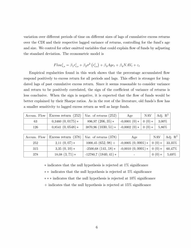
variation over di¤erent periods of time on di¤erent sizes of lags of cumulative excess returns

over the CDI and their respective lagged variance of returns, controlling for the fund�s age

and size. We control for other omitted variables that could explain �ow of funds by adjusting

the standard deviation. The econometric model is

Flowit;s = �1rit;s + �2�

2�rit;s�+ �3Aget + �4NAVt + "t

Empirical regularities found in this work shows that the percentage accumulated �ow

respond positively to excess return for all periods and lags. This e¤ect is stronger for long-

dated lags of past cumulative excess return. Since it seems reasonable to consider variance

and return to be positively correlated, the sign of the coe¢ cient of variance of returns is

less conclusive. When the sign is negative, it is expected that the �ow of funds would be

better explained by their Sharpe ratios. As in the rest of the literature, old funds�s �ow has

a smaller sensitivity to lagged excess return as well as large funds.

Accum. Flow Excess return (252) Var. of returns (252) Age NAV Adj. R2

63 0,3460 (0; 0175) � 896,97 (206; 35) � -0,0001 (0) � 0 (0) � 3,00%

126 0,8541 (0; 0548) � 3870,96 (1030; 51) � -0,0002 (0) � 0 (0) � 5,86%

Accum. Flow Excess return (378) Var. of returns (378) Age NAV Adj. R2

252 2,11 (0; 07) � 1000,45 (652; 98)+ -0,0005 (0; 0001) � 0 (0) � 33,35%

315 3,35 (0; 10) � -2500,68 (141; 18) � -0,0010 (0; 0001) � 0 (0) � 60,47%

378 18,08 (3; 71) � -12780,7 (1840; 41) � - 0 (0) � 5,69%

� indicates that the null hypothesis is rejected at 1% signi�cance

� � indicates that the null hypothesis is rejected at 5% signi�cance

� � � indicates that the null hypothesis is rejected at 10% signi�cance

+ indicates that the null hypothesis is rejected at 15% signi�cance

6

2 The model under full commitment

Consider a risk neutral investor3 who hires a risk averse portfolio manager to invest a share

of his assets4 in an economy that lasts for two periods. We build a binomial model, i.e., there

are two possible states of nature in each period. At the beginning of each period for each node

of the decision tree, the investor decides the percentage of that share to be allocated with

the portfolio manager, 0, H and L. Besides, the contract that regulates this relationship

describes the portion of return, !H and !L, that is paid to the manager in each node of the

decision tree. We still make two assumptions regarding the compensation schedule: 1) the

explicit incentive is stationary; i.e., they do not vary during the life of the contract and 2)

the explicit incentives are multiplied by the implicit incentives. These assumptions bring a

lot of realism to the model since this schedule is the one frequently observed in the industry.

The portfolio manager has a time-separable utility function with impatient parameter,

�, and he is free to decide how to allocate the assets under his management in any possi-

ble investment alternative available in the economy. In order to make these decisions, the

manager exerts costly and unobservable e¤ort. Portfolio manager�s e¤ort decisions represent

his set of feasible investment strategies and appear as more intense access to information,

increased leverage, greater duration of �xed income instruments, open gap and credit risks,

active day-trading, foreign exchange risks, etc. Thus, e¤ort decisions a¤ect the probability

distribution of excess return ex ante, �t;s and they are considered to be non-negative andassume continuous values on the unit interval such that et;s 2 [0; 1].We still assume that the cost function of e¤ort is monotonically increasing and twice

continuously di¤erentiable in e¤ort; such that we have(0) = 0, limes!1

0(et;s) =1;0(�) > 0;00(�) > 0 and 000(�) � 0 which guarantees su¢ ciency conditions for interior solution and

easy calculation of several static comparisons. In order to simplify the algebraic calculations,

we de�ne a quadratic time-separable cost function

(et;s) =k

2(et;s)

2 (1)

The asymmetric information aspect of the model relies in the fact that et;s is unobservable

by the investor. In each period, the two states of nature are associated with two levels of

3The risk neutrality assumption is due to the standard justi�cation that investors can diversify managers�

speci�c risks away while each manager may not.4We do not make any consideration about these assets or their associated markets.

7

excess return. The return of the investments made by the portfolio manager are compared

to a pre-de�ned benchmark return, rb. The investor, then, is not capable to know with

certainty if excess return is due to e¤ort or good fortune (luck). Indeed, the excess return,

rs, is a noisy signal of et;s and the portfolio manager is rewarded only on the basis of this

noisy signal.

In the binomial model, high e¤ort is associated with a higher excess return, rH , and a

particular compensation for the manager, !H . On the other hand, low e¤ort is associated

with a lower level of excess return, rL, and a di¤erent compensation for the manager, !L.

The function that describes the probability of obtaining a particular value of excess return

is linear in e¤ort and it is given by

�t;s = a+ bet;s , 8

8><>:a+ b < 1

a; b > 0

0 � et;s � 1(2)

The e¤ort and parametric restrictions are necessary to avoid negative, equal or greater than

one values of probabilities of return. The coe¢ cients of the function that transforms e¤ort

into the probability of occurrence of a particular state of nature are exogenously given in our

model and they determine the level of informativeness of the noisy signal, rs. The intercept,

a, can be seen as a parameter that only depends on speci�cs characteristics of each portfolio

manager while the slope, b, represents the shift in the distribution of return derived from

variations in e¤ort. The greater is the value of b, the more dependent of e¤ort is probability

distribution of return.

If a � 1 and b � 0, then return is a su¢ cient statistic for highly skilled managers or, wemay say, for speci�c features of the instruments and markets traded by the manager. Hence,

return will only allow the investor to infer about manager�s ability or about the implied risks

of the portfolio; for example, given a particular investment regulation. In this case, moral

hazard would not be an issue. In the case a � 12and b � 1

2, the variance of return will

be high and its level of informativeness will be very low. Therefore, it should neither be

regarded as a good measure to evaluate idiosyncratic manager�s pro�les nor a good proxy of

high levels of e¤ort. On the other hand, when a � 0 and b � 1, then return is a su¢ cientstatistic for high levels of e¤ort decisions executed by the manager and, thus, it should be

used as a proxy of the manager compensation structure in our model. Moral hazard plays

an important role in the maximization problem of the investor and inducing optimal e¤ort

8

increase the value of the relationship.

In the model, expected return as well as variance depend explicitly on e¤ort and are

given by

E [rt;s] = (a+ bet;s) rH � (1� a� bet;s) rL (3)

and

V ar [rt;s] = (a+ bet;s) : (1� a� bet;s) : (rH � rL)2 (4)

thus, expected return and variance are endogenous to e¤ort decisions in our model.The binomial distribution has an interesting relationship between the expected excess

return and its variance. Low e¤ort leads to low expected return and to low variance of returns

as well. As et;s increases and approaches half , both variance and expected return go up while

variance attains its maximum at et;s = 0:5. So, medium e¤ort is related to a greater average

return but maximum variance. As et;s goes to one, expected return reaches its maximum

and variance is at its minimum again, that is, 0. In this model, the distribution of excess

returns conditional on high e¤ort, �t;s, stochastically dominates in �rst-order the distribution

of excess returns conditional on low e¤ort, (1� �t;s). However, in a second-order stochasticdominance sense, the distribution of excess return conditional to low e¤ort dominates the

one conditional to high e¤ort for 0 � �t;s <12. On the other hand, for 1

2� �t;s � 1, the

distribution of excess return conditional to high e¤ort dominates stochastically in a second-

order sense the distribution of excess return conditional to low e¤ort.

In economic terms, e¤ort choice represents the reduced form of two tasks: e¤ort choices

increase expected return and risk choices shift variance of returns. In the interval �t;s 2�0; 1

2

�,

they are substitutes tasks. Only for higher than half e¤ort choices becomes complementary

tasks. Remember that it is less costly to induce complementary tasks than two substitute

tasks in a second best environment since there are economies of scope when these tasks

entails moral hazard. Then, these economies of scope only appear for levels of e¤ort greater

than half.

2.1 The timing of the model and the decision tree

The timing of the two period model is explained as follows. At the beginning of the �rst

period, the investor simultaneously o¤ers a contract f!H ; !L;0g to the portfolio manager

9

that pays fees ! for an initial investment 0. The manager makes an e¤ort decision to de�ne

and execute a particular asset allocation strategy. Then, nature moves and a particular value

of excess return, r1;s, is realized.

At the end of the �rst period, the investor and the portfolio manager observe r0 and,

then, the investor changes 0 to H or L, according to r1;s. In the beginning of the second

period, the manager chooses an state-dependent e¤ort and nature will move again such that

a particular value of excess return, r2;s, is realized.

Time table goes here

Decision tree graph goes here

2.2 The portfolio manager problem: optimal choice of e¤ort

The portfolio manager maximizes expected utility by choosing the optimal levels of e¤ort

maxe0;e1;e2

UM =2Xt=0

�t

24st=rtXst=rt

P (rtjet)u (t;s!t;s)�k

2(et;s)

35 (5)

=

��0u (0!H) + (1� �0)u (0!L)�

k

2(e0)

2

�+�

(�0��1u (H!H) + (1� �1)u (H!L)� k

2(e1)

2�+(1� �0)

��2u (L!H) + (1� �2)u (L!L)� k

2(e2)

2�)

where the utility function of the portfolio manager presents the usual properties of concavity:

u( = 0; ! = 0) = u!( = 0; ! = 0) = 1 lim!1;!!1

u(�; �) = u! (�; �) = 0; u(; !) > 0;u!(; !) > 0; u(; !) < 0; u!!(; !) < 0. Risk aversion creates ine¢ ciencies in the

provision of e¤ort due to the e¤ects of moral hazard and, in this case, the risk neutral

investor should pay a premium for a risk averse manager to participate.

The reservation utility of the portfolio manager is exogenously given and is equal to UM .

The investor has all bargaining power and can make take-it-or-leave-it o¤ers to the portfolio

manager subject to providing him with an expected payo¤ which yields at least UM .

10

Normalizing 0 = 1, we obtain

e�0 =b [u (!H)� u (!L)]

k+ �b

8>>>><>>>>:ka [u (H!H)� u (L!H)]

+k (1� a) [u (H!L)� u (L!L)]

+b2�2k�12k

� " (u (H!H)� u (H!L))2

� (u (L!H)� u (L!L))2

#9>>>>=>>>>; = A (!;)

(6)

e�1 =b [u (H!H)� u (H!L)]

k= E (!;) (7)

e�2 =b [u (L!H)� u (L!L)]

k= I (!;) (8)

Observe that the optimal e¤ort choice in the �rst period has a dynamic component

represented by the present value of the di¤erence in utility that the manager derive in each

of the two possible states of nature in the second period. There are three terms: the �rst

two terms show the di¤erence in utility given distorted incentives weighted by the exogenous

factor representing the manager�s speci�c characteristics, a and k. The greater is a, the

greater is H � L and the greater is !H , the greater is e�o. The third term contains two

quadratic terms representing the di¤erence in utility given distorted incentives weighted by

the level of informativeness of return, b, as well as the cost function parameter, k. That

is, optimal choice in the hidden action problem contains all elements of the compensation

schedule, revealing the power of the implicit incentive in the dynamic moral hazard problem.

For a given a and b, when !H > !L and H > L, the optimal choice of unobservable

e¤ort in the �rst period is higher in the dynamic problem than in the static version. With

enough dynamic incentive H > 0 and enough dynamic penalization L < 0, it is possible

to reduce the cost of implementing second-best solutions with a smaller distortion between

!H and !L, i.e., the power of the explicit contract will be lower than in the static version. The

importance of the implicit dynamic incentive is raised when the limited liability constraint

binds.

In the second and last period of the relationship, the dynamic component vanishes and

only the distortion in the explicit incentives matter for the manager, a solution that is similar

to the static version of the hidden action problem. In fact, memory plays an important role

by di¤erentiating the compensation in each node of the second period. Memory appears

while the implicit incentive depends on the return observed in the �rst period. Then, the

11

optimal e¤ort solution will obey

e�0 (!;) � e�1 (!;) � e�2 (!;) (9)

2.3 The investor problem: optimal provision of incentives

The risk-neutral investor maximizes expected pro�t by choosing the optimal levels of incen-

tives

max!H ;!L;H ;L

e0;e1;e2

VI =

2Xt=0

24st=rtXst=rt

P (rtjet) t;s (rt;s � !t;s)� (t;s) rb

35 (10)

= �00 (rH � !H) + (1� �0) 0 (rL � !L)� 0rb+��0 [�1H (rH � !H) + (1� �1) H (rL � !L)� Hrb]+� (1� �0) [�2L (rH � !H) + (1� �2) L (rL � !L)� Lrb]

where rb is the return of the outside investment alternative of the investor - the benchmark

return can be obtained without any e¤ort and incentive provision. When (H � 1) > 0, theinvestor is borrowing at this benchmark rate and investing the resources in the fund. While

(H � 1) < 0, the investor is withdrawing resources from the fund and re-investing them

in benchmark return-linked instruments. The investor observes excess return at the end

of every period and decides to change the implicit incentive based on the history of excess

returns. Excess return represents a noisy signal of e¤ort with mean and variance respectively

given by (3) and (4).

In equilibrium, the investor anticipates the optimal choice of actions taken by the portfolio

manager and design an incentive compatible contract. When rb = 0, the problem of the

investor becomes

max!H ;!L;H;L

VI = (a+ be�0 (w;)) (rH � !H) + (1� a� be�0 (w;)) (rL � !L)

+� (a+ be�0 (!;)) [(a+ be�1 (!;))H (rH � !H) + (1� a� be�1 (!;))H (rL � !L)]

+� (1� a� be�0 (!;)) [(a+ be�2 (!;))L: (rH � !H) + (1� a� be�2 (!;))L (rL � !L)]

subject to the following participation constraints. We normalize the reservation utility to

12

zero in each node and write8>>>>>><>>>>>>:

�(a+ be�0 (!;))u (!H) + (1� a� be�0 (!;))u (!L)� k

2(e�0 (!;))

2+� (a+ be�0 (!;))

((a+ be�1 (!;))u (H!H)� k

2(e�1 (!;))

2

+(1� a� be�1 (!;))u (H!L)

)

+� (1� a� be�0 (!;))((a+ be�2 (!;))u (L!H)� k

2(e�2 (!;))

2

+(1� a� be�2 (!;))u (L!L)

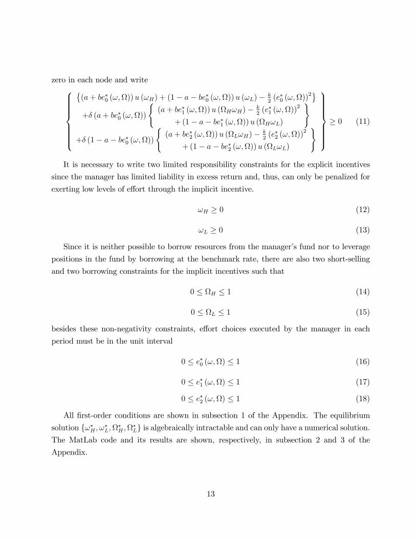
)9>>>>>>=>>>>>>;� 0 (11)

It is necessary to write two limited responsibility constraints for the explicit incentives

since the manager has limited liability in excess return and, thus, can only be penalized for

exerting low levels of e¤ort through the implicit incentive.

!H � 0 (12)

!L � 0 (13)

Since it is neither possible to borrow resources from the manager�s fund nor to leverage

positions in the fund by borrowing at the benchmark rate, there are also two short-selling

and two borrowing constraints for the implicit incentives such that

0 � H � 1 (14)

0 � L � 1 (15)

besides these non-negativity constraints, e¤ort choices executed by the manager in each

period must be in the unit interval

0 � e�0 (!;) � 1 (16)

0 � e�1 (!;) � 1 (17)

0 � e�2 (!;) � 1 (18)

All �rst-order conditions are shown in subsection 1 of the Appendix. The equilibrium

solution f!�H ; !�L;�H ;�Lg is algebraically intractable and can only have a numerical solution.The MatLab code and its results are shown, respectively, in subsection 2 and 3 of the

Appendix.

13

2.4 Characterization of the optimal incentive contract

In equilibrium, the investor o¤ers an incentive compatible contract f!�H ; !�L;�H ;�Lg thatsatis�es all the constraints of his problem. The investor provides total incentives that equalize

the marginal excess expected return and the implied costs of e¤ort induction. He does so

by simultaneously combining and distorting both the implicit and the explicit incentive�s

compensation structure as to maximize the intertemporal excess expected return.

The explicit incentive reduces net excess expected return. When rL < 0, (13) binds and

the investor o¤ers !�L = 0, because of limited liability. In equilibrium, the investor sets

!�H � 0 as to increase the probability of high return in each node of the decision tree. Thisresult is natural since setting !�H > !

�L = 0, induces positive e¤ort, increases the probability

of high return in all nodes of the tree and, thus, increases excess expected return. For a

given solution f�H ;�Lg, the optimal level of performance fee, !�H , equalizes marginal excessexpected return due to shifts in the probability distribution of return to the marginal cost

of exerting e¤ort in all nodes of the tree. Then, the optimal contract is a combination of

f!�H ; 0;�H ;�Lg.Since we are imposing the �rst-order approach (FOA) - by substituting the portfolio

managers��rst-order conditions into the investor�s objective function - it needs to be checked

if the second-order conditions (SOC) satisfy the necessary and su¢ cient conditions for a

local maxima. That is, we verify if at the solution found numerically, f!�H ; !�L;�H ;�Lg, theHessian matrix of the portfolio manager�s maximization problem is negative semi-de�nite.

2.4.1 Comparison with the case where �H = �L = 1

The �ow of funds serves two purposes. First, it determines the investor�s asset allocation

strategy. From a �nance and portfolio allocation perspective, we know that the risk neutral

investor should choose � = 1 if excess expected return is positive. On the other side, when

net excess expected return is negative, the investor sets � = 0.

Due to hidden action considerations, the �ow of funds also plays the role of an implicit

incentive as to avoid moral hazard in the execution of e¤ort. In the dynamic model. the

investor desires to induce greater e¤ort in the �rst period while its bene�ts are greater

than the ones generated by e¤ort executed in the second period. That is, investor faces a

intertemporal trade-o¤ between inducing e¤ort in the �rst period - which increases expected

return in the �rst period - vis-à-vis inducing e¤ort in second period - increasing expected

14

return in the second period. Then, the investor distort the implicit incentive equilibrium

allocations that may di¤er from the natural and trivial solution described above. Then, the

�ow of funds modify the allocation classical rule such that

E [rt;s]� (rb + !�H) > 0) 0 < �t;s � 1

and

E [rt;s]� (rb + !�H) � 0) 0 � �t;s < 1

Moreover, since expected return is endogenous in this model and given (9), we have

E�r�1;0�> �E

�r�1;1�� �E

�r�2;1�

Indeed, there is economic value in providing distorted implicit incentives at the cost of

destroying the relationship in the second period whenever one observes negative excess return

in the �rst period. To maximize expected utility, the investor decides how much endogenous

expected return to give up in the second period in order to obtain endogenous expected

return derived from higher induced e¤ort in the �rst period.

Let�s consider three cases. In the �rst one, there is no distortion in the implicit incentive

such that �H = �L = 1. Then, e¤ort choices will be given by

e�0 = e�1 = e

�2 =

bu (!H)

k� 1 (19)

In this case, ��0 = ��1 = �

�2 = a+ be

� =�a+ b2u(!H)

k

�< 1 and the manager earns

UM = (1 + �)u (!H)

�a+

b2

2ku (!H)

�� 0

In this case, only the explicit incentive, !H , a¤ects e¤ort choices. From (12), the risk averse

manager participation constraints is always greater than zero for all !H > 0 and, hence,

the constraint is not binding (� = 0). On his side, the risk neutral investor earns net excess

expected return

VI = (1 + �)

�a+

b2u (!H)

k

�(rH � rL � !H) + (1 + �) rL > 0 (20)

From (20), the investor problem reduces to choosing !�H . Then, the Lagrangian becomes

L1 = (1 + �)�a+

b2u (!H)

k

�(rH � rL � !H) + (1 + �) rL

15

Optimal choice of !�H will satisfy �rst-order conditions such that

!�H +1

u0 (!�H)

�u (!�H) +

ak

b2

�= (rH � rL) (21)

When we use the CRRA utility function, u (!) = (!)��1

��1 , we have

b2�!�H + ak (�� 1) (!�H)2�� = b2 (�� 1) (rH � rL) (22)

Now, consider a second extreme case. Suppose that the investor o¤ers full implicit

incentive distortion. Then, we have �H = 1 and �L = 0. In this case, e¤ort choices will be

equal to

e�0 =bu (!H)

k

�1 + �

�ak2 +

b2

2(2k � 1)u (!H)

��(23)

e�1 =bu (!H)

k(24)

Then, we have e�0 > e�1 > e

�2 = 0 for k � 1

2.

In this case, the participation constraint is given by

UM =

264 u (!H)�1 + �

�a+ b2u(!H)

2

���a+ b2u(!H)

k

�1 + �

�ak2 + b2u(!H)(2k�1)

2

����u(!H)

2b2

2k

�� +

�1 + �

�ak2 + b2u(!H)(2k�1)

2

��2�375 � 0

(25)

From (25), we can approximately the minimum value of !�H that binds the participation

constraint. If 3b6�2�8b6k�2+4b6k2�2 = 0 and�b4�+ab4�2�2ab4k�2�2ab4k2�2+2ab4k3�2 6= 0,

16

then we can write one possible solution

!�H > u�1

0BBBBBBBBBBBBBBBBBBBBBBBBBBBBBB@

1 +ab4�2 (a� � 1)

�2ab4k�2 (1 + k � k2)

!

0BBBBBBBBBBBBBBBBBBBBBBBBBBBBBB@

0BB@12b2 (1� �)

+ab2��1 + k

2

�+a2b2k2�2

�1� k2

2

�1CCA

�12

vuuuuuuuuuuuuuuuuuuuuuuuut

b4 � 2b4� + 4ab4��6ab4k� + b4�2

�4ab4�2 � 2ab4k�2

+4a2b4�2 + 4a2b4k�2

+8a3b4k�3 � 11a2b4k2�2

�4a2b4k2�3 � 16a2b4k3�2

+14a2b4k4�2 � 8a3b4k2�3

+2a2b4k4�3 � 12a3b4k3�3

+12a3b4k4�3 � 2a3b4k5�3

+4a4b4k4�4 � 4a4b4k6�4

+a4b4k8�4

1CCCCCCCCCCCCCCCCCCCCCCCCCCCCCCA

1CCCCCCCCCCCCCCCCCCCCCCCCCCCCCCA

> 0 (26)

Due to the fact that it reduces the net expected return in all nodes of the tree, we have

!�H < rH . The investor earns an expected return equal to

VI =

a+

b2u (!H)

k

1 + �

ak2

+ (2k�1)u(!H)b22

!!! 1 + �

a

+ b2u(!H)k

!!(rH � rL � !H)(27)

+(1 + �) rL

If (27) > (20) for the same explicit contract, !�H , then it is optimal (in comparison with

the �rst case described above) for the investor to fully distort the contract and o¤er a

compensation scheme with maximum powered implicit incentives. This results follows from

the fact that the marginal bene�t obtained in the �rst period would be greater in module

than the excess expected return given up in the second period. This occurs when � 6=0;�b6� + 2b6k� = 0 and 2b4 � b4k� ab4k� + 2b4k2 + 4ab4k2� 6= 0 such that we can write onepossible solution

17

!�H > u�1

0BBBBBBBBBBBBBBBBB@

1 2b4 � b4k � ab4k�+2b4k2 + 4ab4k2�

!

0BBBBBBBBBBBBBBBBB@

0BBBB@b2k

�2ab2k�ab2k3

�a2b2k3�

1CCCCA

�

vuuuuuuuuut

b4k2 � 2ab4k3 + 2ab4k4

+2a2b4k3 + a2b4k6

�2a2b4k3� + 6a2b4k4�+2a3b4k3� � 4a3b4k4�+2a3b4k6� + a4b4k6�2

1CCCCCCCCCCCCCCCCCA

1CCCCCCCCCCCCCCCCCA

> 0 (28)

From (27), the investor problem reduces to choosing !�H . Then, the Lagrangian becomes

L2 =

a+

b2u (!H)

k

1 + �

ak2

+ (2k�1)u(!H)b22

!!!�1 + �

�a+

b2u (!H)

k

��(rH � rL � !H) (29)

+(1 + �) rL � �

2666664u (!H)

�1 + �

�a+ b2u(!H)

2

�� a+ b2u(!H)

k

1 + �

ak2

+ b2u(!H)(2k�1)2

!!!

�u(!H)2b2

2k

0@� + 1 + � ak2

+ b2u(!H)(2k�1)2

!!21A

3777775Optimal choice of !�H will satisfy �rst-order conditions of the Lagrangian above. The alge-

braic solution here is also intractable and we compare the numerical solution in this case

with the numerical solution in case 1. Please, refer to the next section.

A third possible case is algebraically intractable and it has two possibilities. Either

�H = 1 and 0 < �L < 1 or 0 < �H < 1 and �L = 0. In this two cases, �H > �L and,

then, e�0 > e�1 > e

�2. It often occurs when the investor prefers to o¤er implicit incentive at a

higher cost in terms of giving up positive excess expected returns or seizing negative excess

expected returns. The implicit incentive not only complements the explicit incentive, but it

also substitutes it in inducing e¤ort whenever !�H � 0. On the other hand, variations in theimplicit incentive that are very costly in terms of excess expected return are less intense and

they are compensated by more distortion in the explicit incentive. These results are shown

in the next subsection.

Nevertheless, these results may present some dynamic inconsistency concerns, from the

perspective of the beginning of the second period, since the investor may change his decision

18

and not give up positive excess expected return once e¤ort induced in the �rst period was

already executed and the probability distribution function of returns of the �rst period does

not in�uence the one of the second period. Therefore, implicit incentives distortion would

represent a non-credible threat. We can adopt several strategies to solve this problem. For

example, we may assume that the repeated game is played in�nitely or that reputation

concerns would force the investor to choose this costly allocation strategy.

Another possibility is that this problem may explain the little presence of complex long

term explicit contracts in the asset management industry. That is, the investor writes a

simple long term explicit contract and allows the powerful implicit incentive depend on his

beliefs at each node of the decision tree in each period of the relationship. In other words,

possible agency problems derived from simple and/or incomplete explicit incentives may be

partially solved by delegating extreme power to the implicit incentive. Yet, �ow of funds

concerns complements the performance fee and may correct some wrong incentives and risk

incongruities that may arise with the design of a simple explicit mechanism.

2.5 Numerical results

We assume that the risk aversion manager�s preferences are represented by a constant relative

risk aversion utility function (CRRA) and that the parameter of risk aversion of the function

is �. The utility function is of the form

u (!) =(!)��1

�� 1

The coe¢ cient of relative risk aversion is given by

RR = 2� �

The parameters values of the model are the coe¢ cients a and b of the linear function that

de�nes the probability distribution function of return in each node of the tree. The parameter

of impatience is � and the cost function coe¢ cient is k:The high and low return depend on the

level of the benchmark rate and the number of days as well as on the benchmark percentage

variation of the benchmark return obtained in each state of nature; respectively, rB, days,

19

cdiperchH and cdipercL. We calculate rH and rL in the following way

rH =�(1 + cdi)(days=252) � 1

�� cdipercH

rL =�(1 + cdi)(days=252) � 1

�� cdipercL

rB =�(1 + cdi)(days=252) � 1

�The table shows all parameter values of the basic scenario

k a b � om0 cdi days cdipercH cdipercL rho rH rL rB

8 0.10 0.85 0.90 1.00 15% 252 150% 80% 1.15 22.5% 12.0% 15%

We use the fmincom function of the Optimization toolbox from Matlab. The MatLab

code �les are presented in subsection 2 of the Appendix 2. We make some adjustments in

our problem to be able to solve it numerically. Since the fmincom function is a non-linear

constrained minimization function, we multiply the investor objective function by minus

one. We also have to multiply the participation constraint by minus one since the fmincom

function read inequality constraints as functions smaller or equal than zero.

Given the nonlinearity existent in the problem, the global optimal solution depends on

the initial guess values provided in the computational program. So, we run the code for

several starting points and select the best result that satisfy all the constraint in the model.

Besides, we run the model for several set of parameters. The best result of each set of

parameters is presented in the tables below and in the subsection 3 of the Appendix. The

�rst column indicates the parameter that varies and the respective values of the analysis.

cdiperch wh wl omh oml e0 e1 e2 Man

Exp Util Inv ExpExcRet

PerfFee

(%aa)

E [r0exc](% cdi)

E [r1exc](% cdi)

E [r2exc](% cdi)

1,100 0,5745% 0,00% 98,10% 0,00% 0,897 0,562 0,036 2,1279 0,1333 3,48% 105,884% 97,341% 83,907%1,200 0,9047% 0,00% 100,00% 0,00% 0,985 0,610 0,038 2,3984 0,1540 5,03% 117,489% 104,742% 85,309%1,300 0,9750% 0,00% 100,00% 0,00% 1,000 0,618 0,039 2,4466 0,1762 5,00% 127,500% 111,262% 86,657%1,400 0,9750% 0,00% 100,00% 0,00% 1,000 0,618 0,039 2,4466 0,1985 4,64% 137,000% 117,515% 87,988%1,500 0,9750% 0,00% 100,00% 0,00% 1,000 0,618 0,039 2,4466 0,2208 4,33% 146,500% 123,767% 89,320%1,750 0,9750% 0,00% 100,00% 0,00% 1,000 0,618 0,039 2,4466 0,2764 3,71% 170,250% 139,399% 92,648%2,000 0,9750% 0,00% 100,00% 0,00% 1,000 0,618 0,039 2,4466 0,3321 3,25% 194,000% 155,030% 95,977%

When the cost parameter is lower (k = 4), the e¤ort upper bound restriction binds with only

the implicit incentives full distortion; then, there is no more room for extra explicit incentive

20

distortion and its power is reduced.

cdiperch wh wl omh oml e0 e1 e2 Man

Exp Util Inv ExpExcRet

PerfFee

(%aa)

E [r0exc](% cdi)

E [r1exc](% cdi)

E [r2exc](% cdi)

1,100 0,5002% 0,00% 6,98% 0,00% 0,339 0,185 0,017 1,1978 0,1200 3,03% 91,645% 87,709% 83,443%1,200 0,6076% 0,00% 14,91% 0,00% 0,363 0,214 0,018 1,2700 0,1262 3,38% 96,332% 91,277% 84,611%1,250 0,7732% 0,00% 25,02% 0,00% 0,389 0,241 0,019 1,3527 0,1296 4,12% 99,360% 93,725% 85,216%1,300 0,8396% 0,00% 100,00% 0,00% 0,429 0,301 0,019 1,4695 0,1333 4,31% 103,231% 97,798% 85,807%1,400 1,1018% 0,00% 100,00% 0,00% 0,451 0,316 0,020 1,5496 0,1428 5,25% 108,997% 102,091% 87,015%1,500 1,3441% 0,00% 100,00% 0,00% 0,468 0,326 0,021 1,6125 0,1526 5,97% 114,830% 106,422% 88,225%1,750 1,9894% 0,00% 100,00% 0,00% 0,503 0,349 0,022 1,7487 0,1785 7,58% 130,114% 117,673% 91,278%2,000 2,5895% 0,00% 100,00% 0,00% 0,528 0,365 0,023 1,8502 0,2060 8,63% 145,883% 129,207% 94,348%

As expected return goes up, the implicit incentive grows faster than the explicit incentive.

Observe that, given �rst period incentive considerations, �H > 0 even when E [r1] < 100%

of the benchmark return. As cdiperch goes up, both the implicit incentive and the explicit

incentives are o¤ered. When, the implicit incentive upper bound constraint becomes active,

the explicit incentive becomes more powerful and the performance fee is higher.

a wh wl omh oml e0 e1 e2 ManExp Util

Inv ExpExcRet

PerfFee

(%aa)

E [r0exc](% cdi)

E [r1exc](% cdi)

E [r2exc](% cdi)

0,01 1,7140% 0,00% 100,00% 0,00% 0,533 0,376 0,024 1,4027 0,1508 7,62% 115,764% 105,455% 82,262%0,05 1,5139% 0,00% 100,00% 0,00% 0,502 0,353 0,022 1,4886 0,1514 6,73% 115,098% 105,720% 84,902%0,10 1,3441% 0,00% 100,00% 0,00% 0,468 0,326 0,021 1,6125 0,1526 5,97% 114,830% 106,422% 88,225%0,15 1,1806% 0,00% 100,00% 0,00% 0,435 0,300 0,019 1,7382 0,1542 5,25% 114,841% 107,327% 91,562%0,20 1,0220% 0,00% 100,00% 0,00% 0,402 0,275 0,017 1,8643 0,1564 4,54% 115,107% 108,429% 94,910%0,25 0,8740% 0,00% 100,00% 0,00% 0,370 0,250 0,016 1,9915 0,1590 3,88% 115,633% 109,736% 98,272%0,30 0,7087% 0,00% 100,00% 0,00% 0,336 0,224 0,014 2,1051 0,1621 3,15% 116,304% 111,175% 101,642%0,50 0,2562% 0,00% 100,00% 0,00% 0,210 0,130 0,008 2,5271 0,1805 1,14% 121,630% 119,081% 115,258%

For greater levels of the parameter a, the probability distribution function of return is less

dependent on e¤ort execution; then, the investor�s marginal return obtained with distortion

in the incentive structure is smaller. The implicit incentive distortion with the objective to

induce e¤ort in the �rst period still plays a major role and it is used, even when it is costly

as seen in the two last cases of the table above. The explicit incentive is clearly less and less

signi�cant in the induction of e¤ort as a increases.

delta wh wl omh oml e0 e1 e2 ManExp Util

Inv ExpExcRet

PerfFee

(%aa)

E [r0exc](% cdi)

E [r1exc](% cdi)

E [r2exc](% cdi)

0,75 1,3253% 0,00% 100,00% 0,00% 0,443 0,326 0,021 1,5263 0,1279 5,89% 113,361% 106,375% 88,222%0,80 1,3290% 0,00% 100,00% 0,00% 0,451 0,326 0,021 1,5541 0,1361 5,91% 113,840% 106,384% 88,223%0,85 1,3383% 0,00% 100,00% 0,00% 0,460 0,326 0,021 1,5836 0,1443 5,95% 114,341% 106,407% 88,225%0,90 1,3441% 0,00% 100,00% 0,00% 0,468 0,326 0,021 1,6125 0,1526 5,97% 114,830% 106,422% 88,225%0,95 1,3886% 0,00% 100,00% 0,00% 0,478 0,328 0,021 1,6512 0,1608 6,17% 115,469% 106,530% 88,232%

21

Patient players, represented by greater levels of � (delta), are less willing to trade-o¤expected

return in the �rst period vis-à-vis expected return in the second period. Then, more explicit

incentive is used to induce higher e¤ort. On the other hand, the portfolio manager is also

more interested in smoothing consumption between the two periods.

Rho wh wl omh oml e0 e1 e2 ManExp Util

Inv ExpExcRet

PerfFee

(%aa)

E [r0exc](% cdi)

E [r1exc](% cdi)

E [r2exc](% cdi)

1,05 0,2531% 0,00% 100,00% 2,02% 1,000 0,730 0,600 20,0904 0,2398 1,12% 146,500% 130,429% 122,729%1,10 1,2535% 0,00% 100,00% 0,00% 0,871 0,517 0,082 5,0694 0,1978 5,57% 138,833% 117,780% 91,878%1,15 1,3441% 0,00% 100,00% 0,00% 0,468 0,326 0,021 1,6125 0,1526 5,97% 114,830% 106,422% 88,225%1,20 1,3666% 0,00% 100,00% 0,00% 0,274 0,212 0,005 0,6449 0,1341 6,07% 103,316% 99,601% 87,317%1,25 1,3288% 0,00% 99,85% 0,00% 0,170 0,140 0,001 0,3029 0,1253 5,91% 97,136% 95,329% 87,083%

As rho approaches 2, the manager becomes less risk averse. The more risk averse is the

manager, the more e¢ cient is the usage of the implicit incentive, that is, the �ow of fund�s

power is much greater as the portfolio manager becomes more risk averse. The riskier averse

is the manager, less distortion is needed to induce e¤ort in the �rst period, reducing the

impact of the intertemporal trade-o¤.

cdi wh wl omh oml e0 e1 e2 ManExp Util

Inv ExpExcRet

PerfFee

(%aa)

E [r0exc](% cdi)

E [r1exc](% cdi)

E [r2exc](% cdi)

2,00% 0,1515% 0,00% 100,00% 0,00% 0,315 0,223 0,014 1,0923 0,0185 5,05% 105,725% 100,255% 87,836%6,00% 0,4729% 0,00% 100,00% 0,00% 0,386 0,273 0,017 1,3210 0,0581 5,25% 109,988% 103,219% 88,023%

10,00% 0,8129% 0,00% 100,00% 0,00% 0,426 0,299 0,019 1,4605 0,0994 5,42% 112,373% 104,817% 88,124%15,00% 1,3441% 0,00% 100,00% 0,00% 0,468 0,326 0,021 1,6125 0,1526 5,97% 114,830% 106,422% 88,225%17,50% 1,5847% 0,00% 100,00% 0,00% 0,482 0,336 0,021 1,6677 0,1797 6,04% 115,690% 106,974% 88,260%20,00% 1,8285% 0,00% 100,00% 0,00% 0,495 0,344 0,022 1,7180 0,2070 6,09% 116,461% 107,465% 88,291%23,00% 2,1247% 0,00% 100,00% 0,00% 0,509 0,353 0,022 1,7732 0,2402 6,16% 117,294% 107,992% 88,324%

Here, an interesting result appears. Since the percentage excess return is greater in nominal

terms for greater levels of benchmark rates of return, the investor has more room to distort

the explicit incentive. This in an intuitive result once it makes sense to believe that it is

harder to obtain percentage of the benchmark excess returns when the benchmark return is

greater. For example, one hundred and �fty percent of a twenty percent benchmark rate is

a three percent excess return and for a two percent benchmark rate of return, we are talking

about one percent excess return. Then, greater benchmark returns are related with more

explicitly powerful contracts, or we may say, greater performance fee.

In general terms, the optimal solution shows that the implicit incentive varies signi�cantly

in the second period depending on the expected return in each node. The investor provides

powerful implicit incentives after the observation of high return in the �rst period and the

22

upper bound (14) binds. On the other hand, after low return is observed in the �rst period,

the investor penalizes the manager, withdrawing all or almost all resources from the manager

and (15) binds. The dynamic implicit incentive component is so strong in this model that

this result occurs even if the expected return is positive in the bad state of nature of the

second period.

The intuition behind it is that since both the total payo¤ and the explicit incentives

depend on the amount of implicit incentives, e¤ort induction by using the �ow of funds is

more e¢ cient under a moral hazard framework .

When we compare the results above where the implicit incentive is very powerful with

the results where there are no implicit incentives, �H = �L = 1, we observe that the

participation constraint is also not binding, but the portfolio manager utility is lower, i.e.,

he extracts less rent Second, we observe that, in most cases, the investor is better o¤ with

powerful implicit incentives provision. Exceptions occur when expected excess return is not

very dependent on e¤ort. A third result is counter-intuitive since we would expect that these

two incentives to be substitutes when, in fact, we observe that they complement each other

as seen in the table below.

Case 1omh = oml = 1

k cdi perch wh omh oml wh Portfolio ManagerUtility

Exp Exc RetInvestor

4 1,100 0,5745% 98,10% 0,0000% 0,5662% -0,37691019 1,21%4 1,200 0,9047% 100,00% 0,0000% 0,7550% -0,258287015 1,60%4 1,300 0,9750% 100,00% 0,0000% 0,9455% -0,338027526 2,07%4 1,400 0,9750% 100,00% 0,0000% 1,1358% -0,448752893 2,50%4 1,500 0,9750% 100,00% 0,0000% 1,3247% -0,546413755 2,88%4 1,750 0,9750% 100,00% 0,0000% 1,8022% -0,755549791 3,68%4 2,000 0,9750% 100,00% 0,0000% 2,2795% -0,928484446 4,29%

k cdi perch wh omh oml wh Portfolio ManagerUtility

Exp Exc RetInvestor

8 1,400 1,1018% 100,00% 0,0000% 0,9959% -0,534967768 0,95%8 1,500 1,3441% 100,00% 0,0000% 1,1659% -0,527764911 0,88%8 1,750 1,9894% 100,00% 0,0000% 1,5935% -0,509474206 0,78%8 2,000 2,5895% 100,00% 0,0000% 2,0228% -0,505074626 0,74%

General results Differences(General case - case 1)

23

Case 1omh = oml = 1

k a wh omh oml wh Portfolio ManagerUtility

Exp Exc RetInvestor

8 0,01 1,7140% 100,00% 0,0000% 1,4904% -0,481716979 1,20%8 0,05 1,5139% 100,00% 0,0000% 1,3458% -0,510716683 1,06%8 0,10 1,3441% 100,00% 0,0000% 1,1659% -0,527764911 0,88%8 0,15 1,1806% 100,00% 0,0000% 0,9932% -0,539236223 0,70%8 0,20 1,0220% 100,00% 0,0000% 0,8307% -0,544520965 0,51%8 0,25 0,8740% 100,00% 0,0000% 0,6817% -0,541325017 0,31%8 0,30 0,7087% 100,00% 0,0000% 0,5481% -0,542269271 0,11%8 0,50 0,2562% 100,00% 0,0000% 0,1828% -0,445592361 -0,63%

General results Differences(General case - case 1)

Case 1omh = oml = 1

k delta wh omh oml wh Portfolio ManagerUtility

Exp Exc RetInvestor

8 0,75 1,3253% 100,00% 0,0000% 1,1674% -0,445428255 0,73%8 0,80 1,3290% 100,00% 0,0000% 1,1673% -0,47392575 0,78%8 0,85 1,3383% 100,00% 0,0000% 1,1662% -0,500497143 0,83%8 0,90 1,3441% 100,00% 0,0000% 1,1659% -0,527764911 0,88%8 0,95 1,3886% 100,00% 0,0000% 1,1658% -0,545341519 0,94%

General results Differences(General case - case 1)

Case 1omh = oml = 1

k Rho wh omh oml wh Portfolio ManagerUtility

Exp Exc RetInvestor

8 1,05 0,2531% 100,00% 2,0179% 0,8553% -1,740755222 1,44%8 1,10 1,2535% 100,00% 0,0000% 1,0252% -0,770612308 2,47%8 1,15 1,3441% 100,00% 0,0000% 1,1659% -0,527764911 0,88%8 1,20 1,3666% 100,00% 0,0000% 1,2567% -0,294693162 0,75%8 1,25 1,3288% 99,85% 0,0000% 1,2852% -0,167947353 0,91%

General results Differences(General case - case 1)

Case 1omh = oml = 1

k cdi wh omh oml wh Portfolio ManagerUtility

Exp Exc RetInvestor

8 2,00% 0,1515% 100,00% 0,0000% 0,1474% -0,476938509 0,12%8 6,00% 0,4729% 100,00% 0,0000% 0,4561% -0,520274813 0,34%8 10,00% 0,8129% 100,00% 0,0000% 0,7701% -0,53814865 0,57%8 15,00% 1,3441% 100,00% 0,0000% 1,1659% -0,527764911 0,88%8 17,50% 1,5847% 100,00% 0,0000% 1,3648% -0,530778996 1,05%8 20,00% 1,8285% 100,00% 0,0000% 1,5650% -0,533119151 1,21%8 23,00% 2,1247% 100,00% 0,0000% 1,8056% -0,534978317 1,42%

General results Differences(General case - case 1)

24

An exception for this third result occurs when we have a corner e¤ort solution in the �rst

period. In this case, explicit incentives provision is restricted since the implicit incentive is al-

ready providing all possible e¤ort. However, when we impose no implicit incentive provision,

more explicit incentive provision is allowed and necessary to maximize e¤ort exertion.

3 The model with two types of portfolio managers

Suppose that there two types of portfolio managers in the economy and that they are het-

erogeneous in the ability to generate positive excess return at each period and each node of

the decision tree., � and �. The high ability portfolio manager, �, produce positive excess

return with positive probability in the good state of nature of the binomial model while the

low ability portfolio manager, �, always produces negative excess return and never adds any

value to the relationship. In this case, P (rH j�) > 0 and P�rH j�

�= 0. We adopt a key sim-

pli�cation in the model and make the level of ability unknown to everyone in the economy,

whether the investor or the manager. Therefore, the portfolio manager�s type is an incom-

plete and symmetric information. Only the prior distribution over � is commonly known

and shared by all contracting parties ex ante.5 Since the information is symmetric, there is

no need for investors to o¤er menus of contracts in order to induce workers to self-select.

We further assume that the proportion of � in the economy is � and the percentage of �

is (1� �). In the �rst period, the investor has to infer the probability of return based on

his belief of �. In the second period, the investor uses his belief and the information derived

from the the excess return observed in the �rst period to infer about the portfolio manager�s

type, �. Now, return is a noisy signal of e¤ort and ability.

All the assumptions and notation remain the same unless for a new superscript in each

e¤ort function which indicates the type of the manager. Then, we describe e¤ort as emt;s 2[0; 1] ; � = �;�. In the �rst period, the probability of high return is given by the probability

distribution of return conditional to the portfolio manager�s expected level of ability

�1;0 = P (�) :P (rH j�) + P���:P�rH j�

�= �

�a�1;0 + b

�1;0e

�1;0

�+ (1� �)

�a�

1;0 + b�

1;0e�

1;0

�The investor and the manager observe the realized return in the �rst period and learn

about the manager�s ability. Then, the investor adjusts the posterior distribution of return in5This idea was �rst introduced by Holmstrom (1982a).

25

a Bayesian way to obtain the probabilities of high return in each node of the second period.

�2;2 = P (rH j�)P (�jrL) + P�rH j�

�P��jrL

�=

�a�1;0 + b

�1;0e

�1;0

�P (�jrL) +

�a�

1;0 + b�

1;0e�

1;0

�P��jrL

�while the probability that the manager is of the � or � type given the return observed

in the �rst period are respectively given by P (�jrH) = P (�)P (rH j�)P (�)P (rH j�)+P(�)P(rH j�)

; P��jrH

�=

P(�)P(rH j�)P (�)P (rH j�)+P(�)P(rH j�)

; P (�jrL) = P (�)P (rLj�)P (�)P (rLj�)+P(�)P(rLj�)

and P��jrL

�=

P(�)P(rLj�)P (�)P (rLj�)+P(�)P(rLj�)

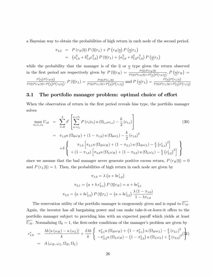
3.1 The portfolio manager problem: optimal choice of e¤ort

When the observation of return in the �rst period reveals hiss type, the portfolio manager

solves

maxe0;e1;e2

UM =2Xt=0

�t

24st=rtXst=rt

P (rtjet)u (t;s!t;s)�k

2(et;s)

35 (30)

= �1;0u (0!H) + (1� �1;0)u (0!L)�k

2(e1;0)

2

+�

8<: �1;0

h�2;1u (H!H) + (1� �2;1)u (H!L)� k

2

�ei2;1�2i

+(1� �1;0)h�2;2u (L!H) + (1� �2;2)u (L!L)� k

2

�ei2;2�2i

9=;since we assume that the bad manager never generate positive excess return, P (rH j�) = 0and P (rLj�) = 1. Then, the probabilities of high return in each node are given by

�1;0 = ��a+ bei1;0

��2;1 =

�a+ b:ei2;1

�P (�jrH) = a+ bei2;1

�2;2 =�a+ bei2;2

�P (�jrL) =

�a+ bei2;2

� � (1� �1;0)1� ��1;0

The reservation utility of the portfolio manager is exogenously given and is equal to UM .

Again, the investor has all bargaining power and can make take-it-or-leave-it o¤ers to the

portfolio manager subject to providing him with an expected payo¤ which yields at least

UM . Normalizing 0 = 1, the �rst-order conditions of the manager�s problem are given by

e�1;0 =�b [u (!H)� u (!L)]

k+��b

k

(��2;1u (H!H) +

�1� ��2;1

�u (H!L)� k

2(e2;1)

2

���2;2u (L!H)��1� ��2;2

�u (L!L) +

k2(e2;2)

2

)(31)

= A (!H ; !L;H ;L)

26

e�2;1 =b [u (H!H)� u (H!L)]

k= E (!H ; !L;H) (32)

e�2;2 =�b�1� ��1;0

�1� ���1;0

[u (L!H)� u (L!L)]k

= I (!H ; !L;L) (33)

Observe that the optimal e¤ort choice in the bad state of nature in the second period

depend on the optimal e¤ort choice in the �rst period. Calculating explicit expressions for

e�1;0 and e�2;2 becomes algebraically intractable and the numerical solution are also provided

for e¤ort choices. Given the Bayesian adjustment of posteriors, we know that e�1;0 > e�2;2

and that e�2;1 > e�2;2. However, we can not say anything about the relation ship between e

�1;0

and e�2;1. As the numerical results show, depending on the parameter values, the di¤erence

between them may have any sign.

3.2 The investor problem: optimal provision of incentives

Now, the risk-neutral investor solves

max!H ;!L;H ;L;

e0;e1;e2

UI = �00 (rH � !H) + (1� �0) 0 (rL � !L) (34)

+��0 [�1H (rH � !H) + (1� �1) H (rL � !L)� (H � 0) rb]+� (1� �0) [�2L (rH � !H) + (1� �2) L (rL � !L)� (L � 0) rb]

subject to the following constraints. We normalize the reservation utility to zero in each

node and write the participation constraint as8>>>>><>>>>>:(a+ be�0 (!;))u (!H) + (1� a� be�0 (!;))u (!L)�

(e�0(!;))2

2

+� (a+ be�0 (!;))

�(a+ be�1 (!;))u (H!H) + (1� a� be�1 (!;))u (H!L)�

(e�1(!;))2

2

�+� (1� a� be�0 (!;))

�(a+ be�2 (!;))u (L!H) + (1� a� be�2 (!;))u (L!L)�

(e�2(!;))2

2

�9>>>>>=>>>>>;� 0

(35)

An incentive compatible contract o¤ered by the investor also satis�es the incentive com-

patibility constraints

e0; e1; e2 2 argmax2Xt=0

�t

"2Xs=1

P (rtjet)u (t;s!t;s)�k

2(et;s)

#(36)

27

The manager has limited liability in excess return and can only be penalized for exerting

low levels of e¤ort through the implicit incentive, reducing the total compensation in the

second-period. Then, it is necessary to write two limited responsibility constraints for the

explicit incentives such that

!H � 0 (37)

!L � 0 (38)

Since it is neither possible to borrow resources from the manager�s fund nor to leverage

positions in the fund by borrowing at the benchmark rate, there are also two short-selling

constraints for the implicit incentives such that

0 � H � 1 (39)

0 � L � 1 (40)

besides these non-negativity constraints, e¤ort choices executed by the manager in each

period must be in the unit interval to avoid probabilities greater than one

0 � e�0 (!;) � 1 (41)

0 � e�1 (!;) � 1 (42)

0 � e�2 (!;) � 1 (43)

The equilibrium solution f!�H ; !�L;�H ;�L; e�0 (!;) ; e�1 (!;) ; e�2 (!;)g is algebraically in-tractable and can only have a numerical solution.

Observe that the investor provides incentives in order to maximize expected utility as

he learns about the manager�s type. For all � < �, it is optimal to o¤er full distortion in

the implicit incentive structure. That is, for a particular belief about the percentage of bad

managers in the economy and below this level, there is no cost in providing full distortion

in the implicit incentive, i.e., when performance is poor in the �rst period, withdrawing all

resources from the fund can be done without any cost.

3.3 Characterization of the optimal incentive contract

In equilibrium, the investor o¤ers an incentive compatible contract f!�H ; !�L;�H ;�Lg thatsatis�es all the constraints of his problem. He also chooses fe�0 (!;) ; e�1 (!;) ; e�2 (!;)g

28

that satisfy the incentive constraints. The investor provides total incentives that equalize

the marginal excess return and the implied costs of e¤ort induction. He does so by simulta-

neously combining and distorting both the implicit and the explicit incentive�s compensation

structure as to maximize the intertemporal excess expected return.

3.4 Numerical results

The table shows all parameter values of the basic scenario

k a b � om0 cdi days cdipercH cdipercL � � rH rL rB

8 0.10 0.85 0.90 1.00 15% 252 150% 80% 1.15 0.8 22.5% 12.0% 15%

The computer codes are presented in subsection 4 of the Appendix. We execute the same

procedure than the one described in the �rst model of this paper. However, due to the

di¢ culties in �nding an explicit solution for e¤ort that we would be able to substitute in the

investor function, the investor now solves the problem for all e¤ort choices as well, having

to respect the incentive constraints from the application of the FOA. Due to calculations

restrictions of the Matlab, we use inequalities near zero for each incentive constraint of e¤ort

choice of the portfolio manager.

The �rst column indicates the parameter that varies and the respective values of the

analysis.

cdiperch wh wl omh oml e0 e1 e2 Man

Exp Util Inv ExpExcRet

Perf Fee(%aa)

E [r0 exc](% cdi)

E [r1exc](%cdi)

E [r2exc](% cdi)

1,300 0,6931% 0,00% 98,77% 0,00% 7,16% 29,08% 3,01% 0,17 (0,0007) 3,55% 86,43% 97,36% 84,88%1,400 0,9980% 0,00% 100,00% 0,00% 32,87% 31,02% 1,44% 1,20 0,1290 4,75% 98,21% 101,82% 84,96%1,500 1,2171% 0,00% 100,00% 0,00% 34,01% 32,09% 1,49% 1,24 0,1352 5,41% 101,79% 106,10% 85,78%1,750 1,7833% 0,00% 100,00% 0,00% 36,31% 34,25% 1,58% 1,33 0,1513 6,79% 111,06% 117,16% 87,86%2,000 2,3401% 0,00% 100,00% 0,00% 38,06% 35,86% 1,64% 1,40 0,1682 7,80% 120,65% 128,58% 89,92%

In the �rst line of the table, �H � 1 because we set �0 = 1 and hence e¤ort induction pays

29

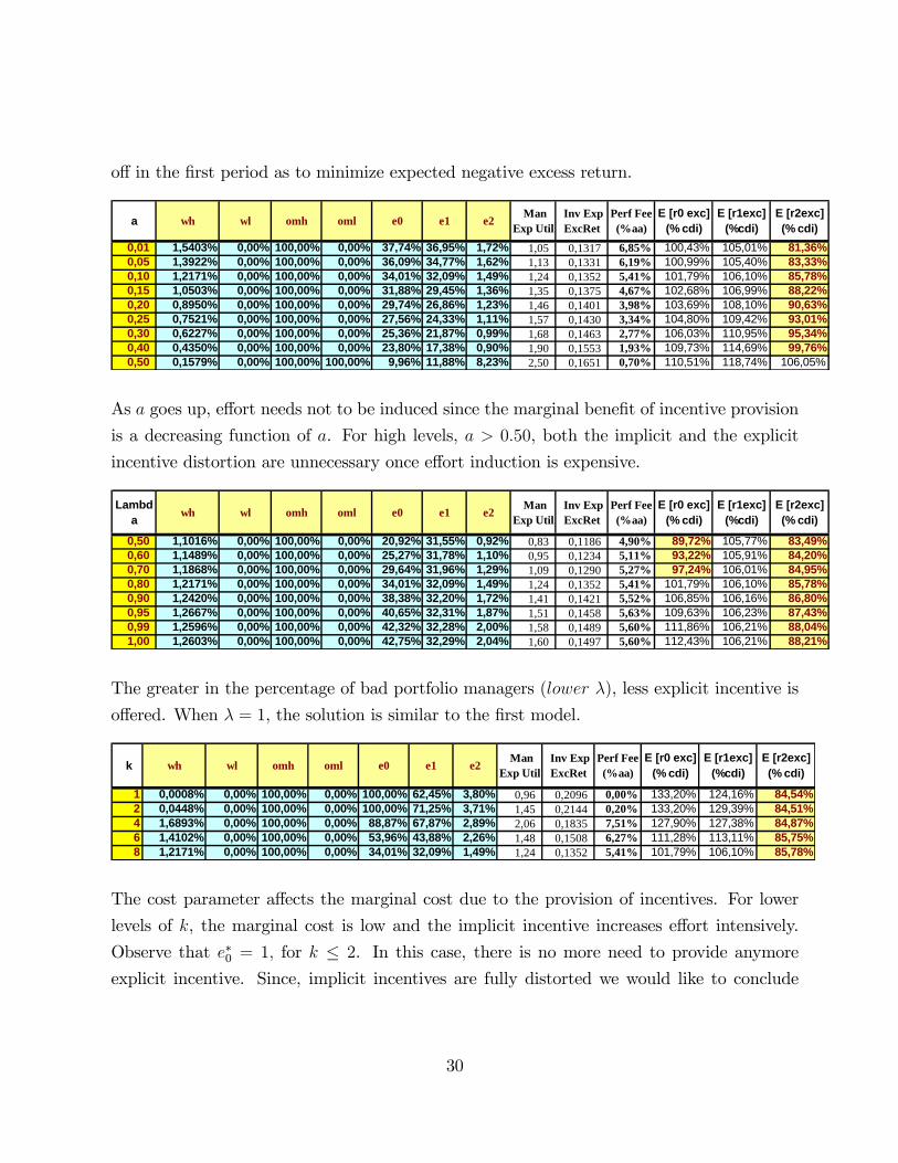
o¤ in the �rst period as to minimize expected negative excess return.

a wh wl omh oml e0 e1 e2 ManExp Util

Inv ExpExcRet

Perf Fee(%aa)

E [r0 exc](% cdi)

E [r1exc](%cdi)

E [r2exc](% cdi)

0,01 1,5403% 0,00% 100,00% 0,00% 37,74% 36,95% 1,72% 1,05 0,1317 6,85% 100,43% 105,01% 81,36%0,05 1,3922% 0,00% 100,00% 0,00% 36,09% 34,77% 1,62% 1,13 0,1331 6,19% 100,99% 105,40% 83,33%0,10 1,2171% 0,00% 100,00% 0,00% 34,01% 32,09% 1,49% 1,24 0,1352 5,41% 101,79% 106,10% 85,78%0,15 1,0503% 0,00% 100,00% 0,00% 31,88% 29,45% 1,36% 1,35 0,1375 4,67% 102,68% 106,99% 88,22%0,20 0,8950% 0,00% 100,00% 0,00% 29,74% 26,86% 1,23% 1,46 0,1401 3,98% 103,69% 108,10% 90,63%0,25 0,7521% 0,00% 100,00% 0,00% 27,56% 24,33% 1,11% 1,57 0,1430 3,34% 104,80% 109,42% 93,01%0,30 0,6227% 0,00% 100,00% 0,00% 25,36% 21,87% 0,99% 1,68 0,1463 2,77% 106,03% 110,95% 95,34%0,40 0,4350% 0,00% 100,00% 0,00% 23,80% 17,38% 0,90% 1,90 0,1553 1,93% 109,73% 114,69% 99,76%0,50 0,1579% 0,00% 100,00% 100,00% 9,96% 11,88% 8,23% 2,50 0,1651 0,70% 110,51% 118,74% 106,05%

As a goes up, e¤ort needs not to be induced since the marginal bene�t of incentive provision

is a decreasing function of a. For high levels, a > 0:50, both the implicit and the explicit

incentive distortion are unnecessary once e¤ort induction is expensive.

Lambda wh wl omh oml e0 e1 e2 Man

Exp Util Inv ExpExcRet

Perf Fee(%aa)

E [r0 exc](% cdi)

E [r1exc](%cdi)

E [r2exc](% cdi)

0,50 1,1016% 0,00% 100,00% 0,00% 20,92% 31,55% 0,92% 0,83 0,1186 4,90% 89,72% 105,77% 83,49%0,60 1,1489% 0,00% 100,00% 0,00% 25,27% 31,78% 1,10% 0,95 0,1234 5,11% 93,22% 105,91% 84,20%0,70 1,1868% 0,00% 100,00% 0,00% 29,64% 31,96% 1,29% 1,09 0,1290 5,27% 97,24% 106,01% 84,95%0,80 1,2171% 0,00% 100,00% 0,00% 34,01% 32,09% 1,49% 1,24 0,1352 5,41% 101,79% 106,10% 85,78%0,90 1,2420% 0,00% 100,00% 0,00% 38,38% 32,20% 1,72% 1,41 0,1421 5,52% 106,85% 106,16% 86,80%0,95 1,2667% 0,00% 100,00% 0,00% 40,65% 32,31% 1,87% 1,51 0,1458 5,63% 109,63% 106,23% 87,43%0,99 1,2596% 0,00% 100,00% 0,00% 42,32% 32,28% 2,00% 1,58 0,1489 5,60% 111,86% 106,21% 88,04%1,00 1,2603% 0,00% 100,00% 0,00% 42,75% 32,29% 2,04% 1,60 0,1497 5,60% 112,43% 106,21% 88,21%

The greater in the percentage of bad portfolio managers (lower �), less explicit incentive is

o¤ered. When � = 1, the solution is similar to the �rst model.

k wh wl omh oml e0 e1 e2 ManExp Util

Inv ExpExcRet

Perf Fee(%aa)

E [r0 exc](% cdi)

E [r1exc](%cdi)

E [r2exc](% cdi)

1 0,0008% 0,00% 100,00% 0,00% 100,00% 62,45% 3,80% 0,96 0,2096 0,00% 133,20% 124,16% 84,54%2 0,0448% 0,00% 100,00% 0,00% 100,00% 71,25% 3,71% 1,45 0,2144 0,20% 133,20% 129,39% 84,51%4 1,6893% 0,00% 100,00% 0,00% 88,87% 67,87% 2,89% 2,06 0,1835 7,51% 127,90% 127,38% 84,87%6 1,4102% 0,00% 100,00% 0,00% 53,96% 43,88% 2,26% 1,48 0,1508 6,27% 111,28% 113,11% 85,75%8 1,2171% 0,00% 100,00% 0,00% 34,01% 32,09% 1,49% 1,24 0,1352 5,41% 101,79% 106,10% 85,78%

The cost parameter a¤ects the marginal cost due to the provision of incentives. For lower

levels of k, the marginal cost is low and the implicit incentive increases e¤ort intensively.

Observe that e�0 = 1; for k � 2. In this case, there is no more need to provide anymore

explicit incentive. Since, implicit incentives are fully distorted we would like to conclude

30

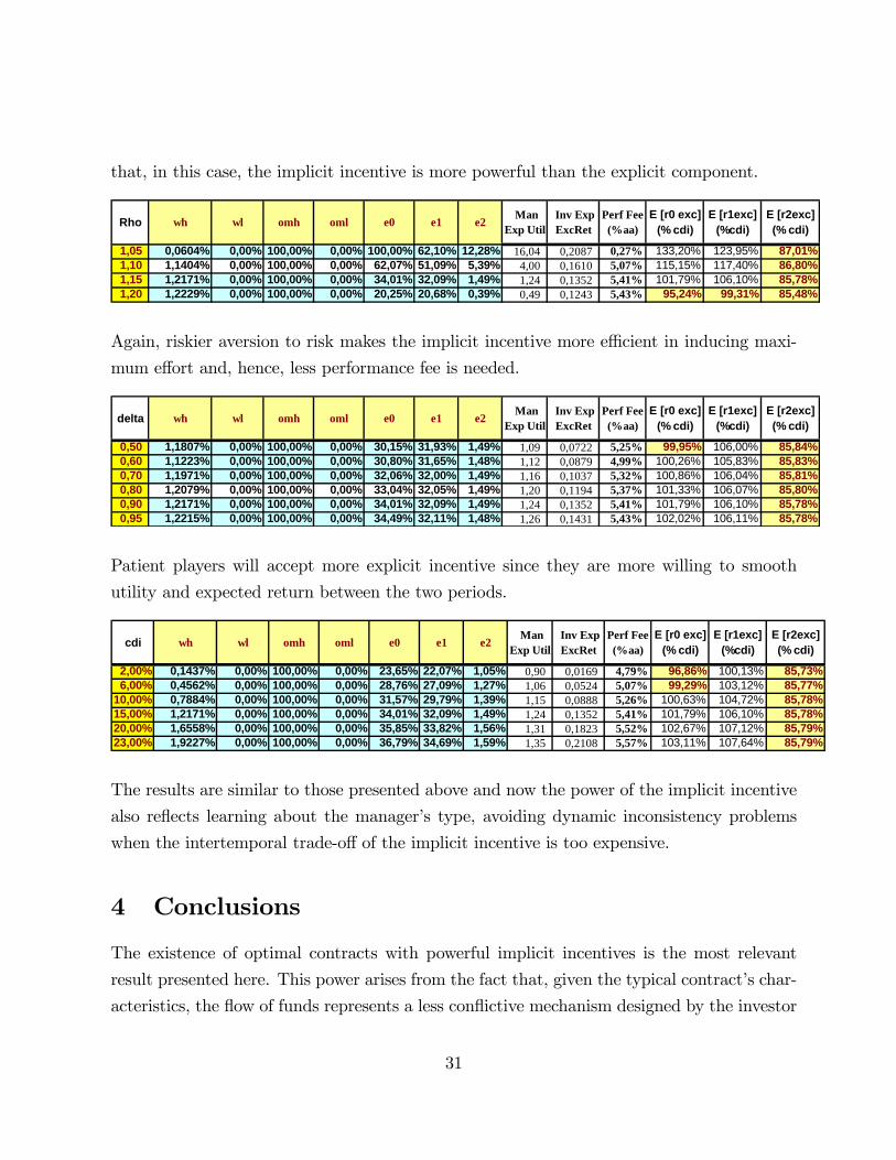
that, in this case, the implicit incentive is more powerful than the explicit component.

Rho wh wl omh oml e0 e1 e2 ManExp Util

Inv ExpExcRet

Perf Fee(%aa)

E [r0 exc](% cdi)

E [r1exc](%cdi)

E [r2exc](% cdi)

1,05 0,0604% 0,00% 100,00% 0,00% 100,00% 62,10% 12,28% 16,04 0,2087 0,27% 133,20% 123,95% 87,01%1,10 1,1404% 0,00% 100,00% 0,00% 62,07% 51,09% 5,39% 4,00 0,1610 5,07% 115,15% 117,40% 86,80%1,15 1,2171% 0,00% 100,00% 0,00% 34,01% 32,09% 1,49% 1,24 0,1352 5,41% 101,79% 106,10% 85,78%1,20 1,2229% 0,00% 100,00% 0,00% 20,25% 20,68% 0,39% 0,49 0,1243 5,43% 95,24% 99,31% 85,48%

Again, riskier aversion to risk makes the implicit incentive more e¢ cient in inducing maxi-

mum e¤ort and, hence, less performance fee is needed.

delta wh wl omh oml e0 e1 e2 ManExp Util

Inv ExpExcRet

Perf Fee(%aa)

E [r0 exc](% cdi)

E [r1exc](%cdi)

E [r2exc](% cdi)

0,50 1,1807% 0,00% 100,00% 0,00% 30,15% 31,93% 1,49% 1,09 0,0722 5,25% 99,95% 106,00% 85,84%0,60 1,1223% 0,00% 100,00% 0,00% 30,80% 31,65% 1,48% 1,12 0,0879 4,99% 100,26% 105,83% 85,83%0,70 1,1971% 0,00% 100,00% 0,00% 32,06% 32,00% 1,49% 1,16 0,1037 5,32% 100,86% 106,04% 85,81%0,80 1,2079% 0,00% 100,00% 0,00% 33,04% 32,05% 1,49% 1,20 0,1194 5,37% 101,33% 106,07% 85,80%0,90 1,2171% 0,00% 100,00% 0,00% 34,01% 32,09% 1,49% 1,24 0,1352 5,41% 101,79% 106,10% 85,78%0,95 1,2215% 0,00% 100,00% 0,00% 34,49% 32,11% 1,48% 1,26 0,1431 5,43% 102,02% 106,11% 85,78%

Patient players will accept more explicit incentive since they are more willing to smooth

utility and expected return between the two periods.

cdi wh wl omh oml e0 e1 e2 ManExp Util

Inv ExpExcRet

Perf Fee(%aa)

E [r0 exc](% cdi)

E [r1exc](%cdi)

E [r2exc](% cdi)

2,00% 0,1437% 0,00% 100,00% 0,00% 23,65% 22,07% 1,05% 0,90 0,0169 4,79% 96,86% 100,13% 85,73%6,00% 0,4562% 0,00% 100,00% 0,00% 28,76% 27,09% 1,27% 1,06 0,0524 5,07% 99,29% 103,12% 85,77%

10,00% 0,7884% 0,00% 100,00% 0,00% 31,57% 29,79% 1,39% 1,15 0,0888 5,26% 100,63% 104,72% 85,78%15,00% 1,2171% 0,00% 100,00% 0,00% 34,01% 32,09% 1,49% 1,24 0,1352 5,41% 101,79% 106,10% 85,78%20,00% 1,6558% 0,00% 100,00% 0,00% 35,85% 33,82% 1,56% 1,31 0,1823 5,52% 102,67% 107,12% 85,79%23,00% 1,9227% 0,00% 100,00% 0,00% 36,79% 34,69% 1,59% 1,35 0,2108 5,57% 103,11% 107,64% 85,79%

The results are similar to those presented above and now the power of the implicit incentive

also re�ects learning about the manager�s type, avoiding dynamic inconsistency problems

when the intertemporal trade-o¤ of the implicit incentive is too expensive.

4 Conclusions

The existence of optimal contracts with powerful implicit incentives is the most relevant

result presented here. This power arises from the fact that, given the typical contract�s char-

acteristics, the �ow of funds represents a less con�ictive mechanism designed by the investor

31

to induce the portfolio manager to exert higher levels of e¤ort. While the implied cost of us-

ing explicit incentives reduce net expected return directly, the implicit incentive only a¤ects

the investor objective function when the benchmark return is greater than the endogenous

expected return obtained by the portfolio manager. The power of the �ow of funds might

also be an explanation for low powered explicit incentives. Indeed, implicit incentives�power

might complement simple explicit incentives, given the general conditions encountered in

the marketplace. Or we may say, powerful implicit incentives may correct some nuisances

created by simple and incomplete linear explicit incentives that are detrimental to e¢ cient

risk choices executed by the portfolio manager.

However, it does not arise as an important incentive response without a relevant implied

cost. First, expected returns are endogenous to e¤ort provision. Second, the trade-o¤

between incentives and performance may be so costly that it even represents a non-credible

threat when the portfolio allocation decision is di¤erent than the usual solution without any

intertemporal incentives consideration.

More importantly, powerful implicit incentives may negatively a¤ect the portfolio man-

ager�s ability to take risks since the implied uncertainty of highly volatile �ow of funds creates

incentives to myopic investing. This greater income uncertainty reduces the utility of a risk

averse manager and may lead to an increase in the likelihood of "closet indexing" of the

fund when past excess return is positive and asset under management grows. On the other

hand, it may also increase the likelihood of excessive risk-taking when past excess return is

negative and the �ow of fund�s expected punishment may lead to all-or-nothing bets.

Rational investors should be "forward looking" decision makers. Since the investor can

not observe e¤ort executed by the manager, moral hazard issues arise and, hence, "backward

looking strategies" maximize expected return. This result may explain an empirical regular-

ity found in the asset management industry that seems to be unreasonable and inconsistent,

once past return may not be indicative of future return.

Indeed, if powerful implicit incentives raise �ow concerns that are detrimental to optimal

e¤ort and risk-taking behavior, it would be desirable to spend time and resources in the

designing of somewhat complex explicit incentives clauses that internalize the history of

returns as well as pre-de�ned variables like investor and portfolio manager�s investment

pro�les and objectives.

For instance, it might make sense to build a compensation structure that depend less

on the total volume under management and design a mechanism in which total incentives

32

are more dependent on performance with a more powerful explicit incentive. The investor

should compensate future performance rather than past performance to guarantee that he

seizes all the possible bene�ts of the dynamic relationship in an asset management contract.

33

5 Appendix

5.1 CPO�s and equations of model in Section 2

Considering that �, �wH , �wL , �H , �L , �1H, �1L , �0, �1, �2, �4, �5, �6 are non-negative

multipliers of the Kuhn-Tucker Lagrangian , the �rst-order conditions for the explicit incen-

tives are given by

� = �

Total exp cost of e¤ort induction given a variation in wHz }| {([AFwH + �: (AEHwH + (1� A) IMwH )] +

+ [AwH�A + � (EwH�E + IwH�I)] + (�0 � �4) :AwH + (�1 � �5) :EwH + (�2 � �6) :IwH

)([APwH + �: (AESwH + (1� A) IVwH )] ++ [AwH�AA + � (EwH�EE + IwH�II)]

)| {z }Total exp mrgl product of e¤ort given a variation in wH

and

� = �

Total exp cost of e¤ort induction given a variation in wLz }| {([(1� A)GwL + � [A (1� E)KwL + (1� A) (1� I)NwL ]] +

+ [AwL�A + � (EwL�E + IwL�I)] +wL +(�0 � �4) :AwL + (�1 � �5) :EwL + (�2 � �6) :IwL

)([(1� A)QwL + � [A (1� E)TwL + (1� A) (1� I)WwL ]] +

+ [AwL�AA + � (EwL�EE + IwL�II)]

)| {z }

Total exp mrgl product of e¤ort given a variation in wL

while the implicit incentives �rst-order conditions are given by

� = �

Total exp cost of e¤ort induction given a variation in Hz }| {f� [AEHH + A (1� E)KH ] + [AH�A + �EH�E] + (�0 � �4) :AH + (�1 � �5) :EHg

f� [AESH + A (1� E)TH ] + [AH�AA + �EH�EE]g| {z }Total exp mrgl product of e¤ort given a variation in H

and

� = �

Total exp cost of e¤ort induction given a variation in Lz }| {(�L+ (�0 � �4) :AL + (�2 � �6) :IL+

+ f� [(1� A) IML + (1� A) (1� I)NL ] + [AL�A + �IL�I ]g

)f� [(1� A) IVL + (1� A) (1� I)WL ] + [AL�AA + �IL�II ]g| {z }

Total exp mrgl product of e¤ort given a variation in L

34

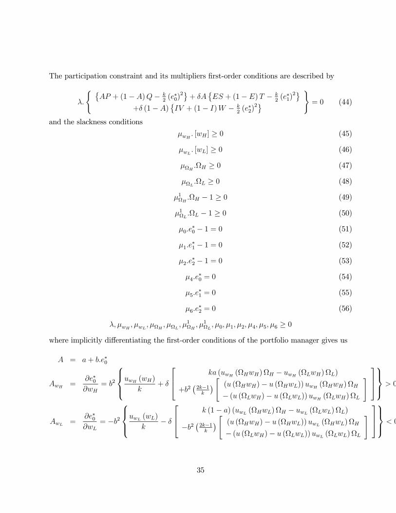
The participation constraint and its multipliers �rst-order conditions are described by

�:

( �AP + (1� A)Q� k

2(e�0)

2+ �A�ES + (1� E)T � k2(e�1)

2+� (1� A)

�IV + (1� I)W � k

2(e�2)

2)= 0 (44)

and the slackness conditions

�wH : [wH ] � 0 (45)

�wL : [wL] � 0 (46)

�H :H � 0 (47)

�L :L � 0 (48)

�1H :H � 1 � 0 (49)

�1L :L � 1 � 0 (50)

�0:e�0 � 1 = 0 (51)

�1:e�1 � 1 = 0 (52)

�2:e�2 � 1 = 0 (53)

�4:e�0 = 0 (54)

�5:e�1 = 0 (55)

�6:e�2 = 0 (56)

�; �wH ; �wL ; �H ; �L ; �1H; �1L ; �0; �1; �2; �4; �5; �6 � 0

where implicitly di¤erentiating the �rst-order conditions of the portfolio manager gives us

A = a+ b:e�0

AwH =@e�0@wH

= b2

8><>:uwH (wH)k+ �

264 ka (uwH (HwH) H � uwH (LwH) L)

+b2�2k�1k

� " (u (HwH)� u (HwL))uwH (HwH) H� (u (LwH)� u (LwL))uwH (LwH) L

# 3759>=>; > 0

AwL =@e�0@wL

= �b2

8><>:uwL (wL)k� �

264 k (1� a) (uwL (HwL) H � uwL (LwL) L)

�b2�2k�1k

� " (u (HwH)� u (HwL))uwL (HwL) H� (u (LwH)� u (LwL))uwL (LwL) L

# 3759>=>; < 0

35

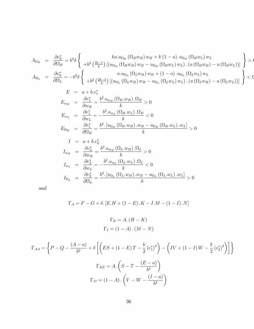
AH =@e�0@H

= b2�

(ka:uH (HwH)wH + k (1� a) :uH (HwL)wL

+b2�2k�1k

�[(uH (HwH)wH � uH (HwL)wL) : (u (HwH)� u (HwL))]

)> 0

AL =@e�0@L

= �b2�(

a:uL (LwH)wH + (1� a) :uL (LwL)wL+b2

�2k�1k

�[(uL (LwH)wH � uL (LwL)wL) : (u (LwH)� u (LwL))]

)< 0

E = a+ b:e�1

EwH =@e�1@wH

=b2:uwH (H :wH) :H

k> 0

EwL =@e�1@wL

= �b2:uwL (H :wL) :H

k< 0

EH =@e�1@H

=b2: [uH (H :wH) :wH � uH (H :wL) :wL]

k> 0

I = a+ b:e�2

IwH =@e�2@wH

=b2:uwH (L:wH) :L

k> 0

IwL =@e�2@wL

= �b2:uwL (L:wL) :L

k< 0

IL =@e�2@L

=b2: [uL (L:wH) :wH � uL (L:wL) :wL]

k> 0

and

�A = F �G+ �: [E:H + (1� E) :K � I:M � (1� I) :N ]

�E = A: (H �K)

�I = (1� A) : (M �N)

�AA =

�P �Q� (A� a)

b2+ �

��ES + (1� E)T � k

2(e�1)

2

���IV + (1� I)W � k

2(e�2)

2

���

�EE = A:

�S � T � (E � a)

b2

��II = (1� A) :

�V �W � (I � a)

b2

�

36

The utility function of the investor and its respective derivatives to all arguments in each

node of the model are given by

F = (rH � wH) =) FwH = �1 < 0G = (rL � wL) =) GwL = �1 < 0

H = H : (rH � wH) =)

8><>:HwH = �H < 0

HH = (rH � wH)(> 0, if rH > wH< 0, if rH < wH

K = H : (rL � wL) =)

8><>:KwL = �H < 0

KH = (rL � wL)(> 0, if rL > wL< 0, if rL < wL

M = L: (rH � wH) =)

8><>:MwH = �L < 0

ML = (rH � wH)(> 0, if rH > wH< 0, if rH < wH

N = L (rL � wL) =)

8><>:NwL = �L

NL = (rL � wL)(> 0, if rL > wL< 0, if rL < wL

while the utility function of the manager and its respective derivatives to all arguments in

each node of the model are given by

P = u (wH) =) PwH = uwH (wH) > 0

Q = u (wL) =) QwL = uwL (wL) > 0

S = u (H :wH) =)(SwH = uwH (H :wH) :H > 0

SH = uH (H :wH) :wH > 0

T = u (H :wL) =)(TwL = uwL (H :wL) :H > 0

TH = uH (H :wL) :wL > 0

V = u (L:wH) =)(VwH = uwH (L:wH) :L > 0

VL = uL (L:wH) :wH > 0

W = u (L:wL) =)(WwL = uwL (L:wL) :L > 0

WL = uL (L:wL) :wL > 0

37

5.2 Computer code for the binomial model

See Matlab prints at the end of this document.

5.3 Computer code for the binomial model with learning

See Matlab prints at the end of this document.

5.4 The typical compensation - linear schedule with limited lia-

bility and high-water mark

In this section we describe the most common asset management contracts found in the

market place. This section serves the purpose to describe possible problems arising from the

use of simple explicit compensation schemes.

Typical explicit clauses of contracts are linear with �xed coe¢ cients during the life ofthe relationship and the payo¤ of the manager depends on the excess return of the fund, rt.

Long-term contracts are unusual. When they do exist, their maturities are de�ned in terms

of the number of days from the withdrawal request to the delivery of the resources back to

the investor. This period is rollover everyday after the lockup period. Then, we will assume

that such contract do not exist in our economic environment.

Actually, given some features in the explicit compensation structure, the contract is not

linear. First, it presents limited liability in the excess return - calculated as the return of the

fund, Rt, in excess of the return of a pre-determined benchmark, R0t . Second, performance

fee is calculated over the high-water mark of the benchmark; that is, performance fee is only

paid if the return exceeds the greater of the two benchmarks - the benchmark itself or the

highest historical quota value of the fund which is also always indexed by the benchmark as

well. Then, the explicit incentive is convex in excess return and the payo¤ can be written as

wt(rt) = t�1�rt�1

�: f�+ �:max [rt; 0]g (57)

where t�1 (rt�1) is the total amount of assets under management and rt�1 = (r1; :::; rt�1)

represents the history of cumulative excess return of the fund over the high-water mark.

We call the total amount of asset under management, in period t, of Net Asset Value

(NAV) and write it as

t�1�rt�1

�= qt�1

�rt�1

�:pt�1 (58)

38

where qt�1 (rt�1) is the outstanding number of quotas of the fund and pt�1 (rt�1) is the

marked-to-market quota value of the fund net of taxes and transactions costs. In period t,

it is given by

pt = p0:tYs=1

(1 +Rs) (59)

The excess return of the fund in period t is given by

rt =ptp̂t� 1 (60)

where the denominator is the high-water quota price. This extra feature of the contract is

given by

p̂t =�1 +R0t

�:max (pt�1; p̂t�1) (61)

Therefore, the high-water mark is given by

brt�1 = max �0;�1� pt�1p̂t�1

��(62)

The manager�s static payo¤consists of a �xed, � - the management fee - and an option on

the value of the fund due to the existence of limited liability - the performance fee, �. From

a �nance theory perspective, this payo¤ is always greater than zero and it synthesizes an

European call option on the fund�s quota mark-to-market price that the portfolio manager

holds against the investor6.

The high-water mark, brt�1, determines the strike price of the option. Because of thehigh-water mark feature and the growth rate of the benchmark, this option has a variable

strike price7. The high-water mark guarantees that the option is almost certainly out-of-the

money since bpt�1 � pt�1. The option is, at maximum, at-the money when bpt�1 = pt�1, i.e.,brt�1 = 0. The distance between pt�1 and bpt�1 determines how much the option is out-of-themoney. So, the greater is bpt�1, the higher is brt�1 and this implies that rt = brt�1 > 0 is

the minimum rate of excess return that the manager need to achieve from his investments

decisions in order to start deriving any positive marginal utility from the option.

From Braido and Ferreira (2003), we learn that options may robustly induce risk-taking,

regardless of the speci�c functional form of the utility function. Higher strike prices trans-

form a riskier portfolio selection that is a second-order stochastically dominated cumulative6See Goeztman, Ingersoll and Ross (2000)7Even when the benchmark is zero, the high-water mark feature incorporates all the variability of the

fund�s history of return.

39

distribution of excess return into a lottery that �rst-order stochastically dominates all other

portfolio choices, even if the excess return probability joint distribution is unknown to the

manager/investor. It means that the likelihood of the portfolio manager to choose riskier

strategies is greater when his compensation includes an option whose strike price is high

enough.

From an incentives theory approach, this out-of-the-money option8 represents a compen-

sation structure in which the manager derives higher marginal bene�ts of exerting e¤ort and

taking risks from high levels of excess return. The manager has incentives to take more risks,

if �t (t�1 (rt�1)) represents a mean preserving spread of the distribution of cumulative ex-

cess return. That is, the manager has incentives to make portfolio choices whose joint prior

distribution of excess returns has heavier tails.

Nevertheless, the high-water mark feature is designed to protect the investor from paying

excessive performance fees. Suppose the manager performs very well during a certain period

of time and the value of the fund hits a record value. Now, imagine that the fund has negative

performance in some subsequent periods. In this case, all positive performance that follows

the poor performance period will only pay performance fee after the record high-water mark

is broken again. Nevertheless, due the option-like nature of the compensation schedule, this

contract feature ends up creating more incongruities in risk preferences between managers

and investors. Benchmarks with high growth rates only enhance this one problem once the

high-water mark will also grow at this rate.

Ghatak and Pandey (2000) build a multi-task model in which the choice of e¤ort moves

the average of the distribution of excess returns, in a �rst-order stochastic dominance sense,

and that the risk choice is a mean preserving spread of this distribution, in a second-order

stochastic dominance sense. Then, the incentive implications of risk-taking choice reduces

the optimal power of the static contract, especially in the presence of limited liability. This

reduction in the explicit incentive, �, objectives to diminish the marginal utility of the

manager from high levels of return, inducing him to choose less risky investment alternatives.

In their model, the optimal linear contract (��; ��) recovers the �rst-best solution, that is,

manager�s actions are equal to the optimal combination of these weakly substitutes tasks in

the case they are contractible.

We would expect that, depending on the strike price of the option, the optimal power of

8And, we may say, increasingly outer-of-the-money if performance is poor or if the growth rate of the

benchmark is high.

40

the contract, �, would change as the value of fund is closer or outer-of-the-money. Moreover,

(��t ; ��t ) also should be a function of the history of performance. Rogerson (1985), in a

repeated moral hazard model, shows that memory plays a crucial role in determining future

incentives if the distribution of today�s return a¤ect current incentives. However, in the asset

management industry, we know that � and � are �xed at the start of the fund. This fact

ampli�es perverse incentives on risk choices, forcing the investor to use implicit features of

the contract in order to recover an optimal compensation schedule and, hence, optimal e¤ort

and risk choices.

As a consequence, the investor has to monitor the performance of each manager and

constantly revise the total amount of assets under management allocated at each portfolio

manager. This is done by adjusting the �ow of funds ft. This �ow is endogenous in the

model and we build it as a function of the history of cumulative excess return, ft (rt). As

investors decide to let cash resources �ow in, ft > 0, or out, ft < 0, of the fund, quotas are

respectively created, �qt > 0, or redeemed, �qt < 0, at current quota marked-to-market

prices, pt.

Then, the total number of quotas in period t� 1 is given by

qt�1�rt�1

�=

t�1Xs=1

fs (rs)

ps(63)

We obtain the �ow of funds in each period t, ft (rt), as a function of the cumulative

return of the fund and the variation in the number of quotas

ft�rt�= pt:

�qt�rt�� qt�1

�rt�1

��(64)

Normalizing p0 = 1 and after substituting (57) in (64), we obtain

ft�rt�=

tYs=1

(1 +Rs) :�qt�rt�� qt�1

�rt�1

��(65)

The �xed fee in the contract, the management fee �, is a factor expressed in annual

percentage terms of the net asset value, t�1 (rt�1), being accrued in a pro rata temporis

form. It is related to the �xed and some variable costs of managing the fund, including the

marginal cost of using the manager�s time9 and/or ability. Once ft (rt) is a function of the

9If we consider leisure in the model. However, we do not do so here

41

history of cumulative excess returns, even in the absence of any performance fee, � = 0, the

manager would still have incentives to make e¤ort and risky choices, trying to in�uence the

perception of the market about his level of ability. Besides, t�1 (rt�1) also multiplies the

option-like component of the manager�s wage, a¤ecting more intensively the e¤ort and risk

choices of the manager in each period. Then, the manager has great incentives to attract a

high volume of assets under management.

Indeed, we argue that the �ow of funds is the most important incentive feature of the

compensation schedule. This dynamic implicit incentive depends on the history of cumulative

excess returns, ft (rt), and we call it �ow concern.This function determine the optimal choices of e¤ort and risk as well as the optimal

incentives, taking into consideration reputation e¤ects that arise from the observed history

of excess returns. Fama (1980) argues that this dynamic concern may recover �rst-best

solutions removing moral hazard issues in risk-taking. Holmström (1982) demonstrated that

risk-aversion and discounting play an important role in con�rming Fama�s previsions.

If we substitute (59) and (61) in (60), we can rewrite the excess return of the fund in

period t as

rt =

tQs=1

(1 +Rs)

(1 +R0t ) :max

�t�1Qs=1

(1 +Rs) ; p̂t�1

� � 1 (66)

Observe that p̂t is calculated recursively based on the history of cumulative excess return,

rt.

We may write the total payo¤ of the manager in each period t as

uM (wt(rt)) = t�1�rt�1

�:

0BB@�+ �:max2664 p0:

tQs=1

(1 +Rs)

(1 +R0t ) :max (pt�1; p̂t�1)� 1; 0

37751CCA

Since the main objective of this paper is to address the relative importance of implicit

incentives compared to explicit incentives,we assumed a general form of explicit incentive,

!H and !L, in the model developed below.

42

References

[1] ARAUJO, A., MOREIRA, H., TSUCHIDA, M. (2004), �The trade-o¤ between incen-

tives and endogenous risk�, EPGE Ensaios Econômicos, no 523

[2] BASAK, S., PAVLOVA, A., SHAPIRO A. (2003), "O¤setting the incentives: Risk Shift-

ing and Bene�ts of Benchmarking in Money Management", MIT Finance Lab Papers,

April 2003

[3] BERK, J. ; GREEN, R. (2004), �Mutual fund �ows and performance in rational mar-

kets�, Journal of Political Economy, Vol. 112, No. 6. (Dez., 2004), pp. 1269-1295

[4] BOLTON, P. , DEWATRIPONT, M. (2005), Contract Theory; MIT Press

[5] BRAIDO, L. AND FERREIRA, D. (2003), �Options can induce Risk taking for Arbi-

trary Preferences�, mimeo, EPGE-FGV

[6] BRAIDO, L. (2004), �Evidence of the relationship between incentives and Exogenous

Risk�, mimeo

[7] CAMPBELL, J. AND VICEIRA, L. (2002), Strategic Asset Allocation � Portfolio

Choice for Long-term investors; Oxford University Press

[8] CARPENTER J. (2000), �Does Option Compensation Increase Managerial Risk Ap-

petite?�, The Journal of Finance, Vol. 55, No. 5. (Oct., 2000), pp. 2311-2331

[9] CHEVALIER, J., ELLISON, G. (1997), �Risk Taking by Mutual Funds as a Response

to Incentives�, The Journal of Political Economy, Vol. 105, No. 6. (Dec., 1997), pp.

1167-1200

[10] DEWATRIPONT, M., JEWITT, I., TIROLE, J. (1999), �The Economics of Career

Concerns, Part I: Comparing Information Structures�, Special issue �Contracts; Review

of Economic Studies

[11] GATHAK, M. AND PANDEY, I (2000), �Contract choice in agriculture with joint

moral hazard in e¤ort and risk�, Journal of Development Economics, 63, 303-326

[12] GOETZMANN W.; BROWN S. (1995), �Performance Persistence�, The Journal of

Finance, Vol. 50, No. 2. (Jun., 1995), pp. 679-698

43

[13] GOETZMANN W.; BROWN S.; IBBOTSON R. (1999), �O¤shore Hedge Funds: Sur-

vival and Performance, 1989-95�, The Journal of Business, Vol. 72, No. 1. (Jan., 1999),

pp. 91-117

[14] GOETZMANN, W., INGERSOLL, J. JR., ROSS S. (2001), �High-Water Marks and

Hedge Fund Management Contracts�, April 18, Yale ICF Working Paper No. 00-34

[15] HEINKEL, R. AND STOUGHTON, N. (1994), �The dynamics of portfolio management

contracts�, Review of Financial Studies, vol. 7, no 2, 351-387

[16] HOLMSTRÖM, B. (1979), �Moral Hazard and Observability�, Bell Journal of Eco-

nomics, 10, 74-91

[17] HOLMSTRÖM, B. (1982A), �Managerial Incentive Problems: A Dynamic Perspective�,

Special issue �Contracts; Review of Economic Studies 1999 ( Reprint)

[18] HOLMSTRÖM, B. AND MILGROM, P. (1987), �Aggregation and linearity in the pro-

vision of intertemporal incentives�, Econometrica, 55, 303-328

[19] HOLMSTRÖM, B. AND MILGROM, P. (1991), �Multi-task Principal-Agent Analyses:

Incentive Contracts, Asset Ownership, and Job Design�, Journal of Law, Economics &

Organization, 7,24-52

[20] LAFFONT, J.J. AND MARTIMORT D. (2002), The theory of incentives � The

principal-agent model; Princeton University Press

[21] LEVIN, J. (2003), "Relational incentive contracts", American Economic Review, 93,

835-857

[22] MACHO-STADLER I. AND PÉREZ-CASTRILLO J. (2001), An introduction to the

Economics of Information �Incentives and Contracts; Oxford University Press

[23] PENDERGAST, C., (2000), �What Trade-O¤ of Risk and Incentives?�, The American

Economic Review, Vol. 90, No. 2, Papers and Proceedings of the One Hundred Twelfth

Annual Meeting of the American Economic Association. (May, 2000), pp. 421-425.

[24] PENDERGAST, C., (2002), �The tenuous trade-o¤ between risk and incentives�, Jour-

nal of Political Economy, 110(5), 1071-1102ROGERSON, W. (1985A), �The First

Order-Approach to principal agent problems�, Econometrica, 53, 69-76

44

[25] SIRRI, E. AND TUFANO, P. (1998), �Costly Search and Mutual Fund Flows�, The

Journal of Finance, Vol. 53, No. 5. (Oct., 1998), pp. 1589-1622

[26] STARKS, L. (1987), �Performance Incentive Fees: An Agency Theoretic Approach�,

The Journal of Financial and Quantitative Analysis, Vol. 22, No. 1. (Mar., 1987), pp.

17-32

[27] STARKS, L.; BROWN, K.; HARLOW, W. (1996), �Of Tournaments and Temptations:

An Analysis of Managerial Incentives in the Mutual Fund Industry�, The Journal of

Finance, Vol. 51, No. 1. (Mar., 1996), pp. 85-110

[28] STOUGHTON, N. (1993), �Moral hazard and the Portfolio Management Problem�,

The Journal of Finance, Vol. 48, no 5, 2009-2028

45