Operation of a Shell and Tubes Heat Exchanger: …...Operation of a shell and tubes heat exchanger 137 2.5 Simulation The SolidWorks2 software was used to simulate the heat exchange

Contemporary Engineering Sciences, Vol. 12, 2019, no. 3, 131 - 147HIKARI Ltd, www.m-hikari.com

https://doi.org/10.12988/ces.2019.9618

Operation of a Shell and Tubes Heat Exchanger:

Process Simulation1

Paul Bolıvar Torres-Jara

Universidad Politecnica Salesiana, Sede CuencaCalle Vieja 12-30 y Elia Liut, Cuenca, Ecuador

Diego Rafael Lasso-Lazo

Universidad Regional Amazonica IKIAMKm 7, vıa a Alto Tena, Ciudad de Tena, Napo, Ecuador

Efren Vazquez-Silva


Gabriela Abad-Farfan


Juan Carlos Galarza-Galarza

INDURAMAAv. Don Bosco y Av. de Las Americas, Cuenca, Ecuador

This article is distributed under the Creative Commons by-nc-nd Attribution License.

Copyright c© 2019 Hikari Ltd.

1The authors are grateful to the Energy Systems Optimization Laboratory (LOSE),Department of Energy, Faculty of Engineering of Guaratingueta, Institute of Bioen-ergy Research (IPBEN), Pualista State University ”Julio de Mesquita Filho” (UNESP),Guaratingueta - SP / Brazil. This institution facilitated its license of SolidWorks software.Thanks to a stay of Engineer Juan Carlos Galarza Galarza, graduate of the UPS, in thementioned laboratory, it was possible to obtain the results of the simulation

132 Paul Bolıvar Torres-Jara et al.

Abstract

The thermo-fluid laboratory at the El Vecino campus of the Sale-siana Polytechnic University in Cuenca (UPS), Ecuador, has a shell andtube heat exchanger. This experimental equipment is very importantfrom the didactic point of view for subjects such as Fluid Mechanicsand Heat Transfer (subjects that are part of the curriculum of the un-dergraduate program of Mechanical Engineering), as well as to carryout application projects at the institutional level. This paper presentsthe results of the simulation of heat transfer processes that take placein the heat exchanger, and demonstrates the feasibility of ”replacing”the physical equipment by the computer simulation. In addition, areshown the benefits that this possible replacement has for the institutionand teaching.

Keywords: Heat exchanger, computer simulation, heat transfer

1 Introduction

Heat exchangers are devices that enable the heat transfer between two fluids atdifferent temperatures without them mixing. These devices are fundamentalelements in heating, cooling, air conditioning, energy production and chemicalprocessing systems; therefore, they are used in all types of industries [1, 2].Approximately 37% of the heat exchangers used for industrial purposes areshell and tubes exchangers [3]. An outer shell, by which one of the fluids flow,as well as several tubes through which the other fluid flows, without them mix-ing, makes up these exchangers. The equipment works by heat transfer due toconduction and convection. In Chemical Industry, where heat transfer withoutcombustion is required, this type of heat exchanger is essential. In this regard,there are different methods for its design and this leads to a line of researchon such devices. For example, in [4] it is possible to find the description andautomation of the Taborek method, used in order to design a heat exchangerof this type. In addition, the design cost is optimized with the application ofthe methods Simulated Annealing and Genetic Algorithms. From the pointof view of the applications, the research conducted on heat exchangers havebeen aimed at increasing the efficiency of this devices under different condi-tion of the surrounding environment [5], and to make this possible, computertools have also been used to develop simulations of state behavior of a heatexchanger.We also found the report by J. Ardalia and his partners [6]. They validatean ANSYS numerical model for the analysis of heat transfer in straight, heli-cal, smooth and torsioned concentric tube exchangers; comparing the obtainedresults with experimental data published in specialized scientific books. Ac-cording to their conclusions, the increase of heat transfer is associated to the

Operation of a shell and tubes heat exchanger 133

geometry of the exchanger. Conclusions of these types of studies have beenthe basis to improve both the design and the terms of use. They have alsohelped save financial resources. It is also possible to cite the works of Cor-rea and Marchetti [7], who compared the behavior of three different shell andtube exchangers to find the most effective. They used an artificial network(ANN) to validate theirs experiments, and the maximum deviation they ob-tained was 2%. On the other hand, Nellis et al. [8] used simulation to validatethe experimental results for heat exchangers used in refrigeration, specificallyin evaporators and condensers. Comparatively they acted within a margin of10% and then used simulation to predict the improvement in the efficiency ofthe exchanger by up to 8.3%.Kamaris et al. ([9]) applied a computational fluid dynamics (CFD) code tosimulate the heat transfer in a plate exchanger. They validated the obtainedresults in an experimental manner and demonstrated the effectiveness of theCFD code for simulation. While J. Judge and R. Radermacher [10] used simu-lation data, to develop a heat exchanger model to cool residential heat pumps.The results improved efficiency by 44% and were validated for four differenttypes of refrigerant. Cordova-Tuta and Fuentes Dıaz [11] develop a computertool for the simulation of flow behavior in the tube and fin exchangers when aphase exchange may occur in the refrigerant. In this case, the finite volumesmethodology was used for the modeling of the exchanger, and the represen-tation of the tube connections was done by means of the graph theory. Withthis model, it was possible to predict the behavior of an evaporator’s flowswhen having dry and wet fins; the error was less than 6% with respect tothe experimental data. Another application of virtual tools for the study ofexchangers is, for example, the use of Hysys. In [12] it is described the val-idation of the linear multivariable control designs in a heat exchanger underthis virtual environment. The study aimed at analyzing the different responsesof the MIMO system, under regulatory control with different uncouplers andwithout uncouplers.The validations of the experimental results have also carried out by applyingthe numerical methods. Anica Trp [13] conducted comparisons between thenumerical and experimental results of the heat transfer in an exchanger as theone being discussed in the present report. Additionally, there is the work ofMachuca and Urresta [14], which presents the structure of a software devel-oped for teaching and learning the dynamics and control of a shell and tubesheat exchanger. The program presents, in a numeric and graphic manner, thedynamic behavior in open and closed loop of the process for different param-eters of design and variable conditions of operation. For a more complete anddetailed information on current issues regarding heat exchangers, the mainlines of research and challenges, you can consult the work of Reyes-Rodrıguezand Moya-Rodrıguez [15].


In our case, we deal with a laboratory equipment, fundamentally used forteaching purposes in the subjects of Fluid Mechanics and Heat Transfer. There-fore, the following question arises: How do we guarantee the laboratory prac-tices in Fluid Mechanics and Heat Transfer when, for some reason, the ex-changer is out of service? An answer to the aforementioned question will begiven. Hence, the following section describes the materials and methods usedto conduct the research. Then, section 3 presents the results of the developedsimulation, which describes the processes that take place in the exchanger,and we made a comparison with the data obtained experimentally. Finally,the conclusions are set forth in section 4.

2 Materials and methods

2.1 Experimental issue

The Shell and Tubes heat exchanger analyzed in this work is a teaching modelof the thermo-fluids laboratory of the Universidad Politecnica Salesiana. Arm-field (Engineering Teaching & Research Equipment) built it. Its characteristicsare shown in Table 1.

Table 1: Technical characteristics of the Shell and Tubes Exchanger

Characteristic Description

Brand ArmfieldNumber of tubes 7Material of the tubes Stainless steelLenght of the tubes 144 mmExternal diameter of the tubes 6.35 mmInternal diameter of the tubes 5.15 mmMaterial of the Shell AcrylicNumber of deflectors 2Material of deflectors Acrylic

Figure 1 shows the constructive aspect of the device, it has thermocouplesto measure the inlet and outlet temperature of the fluid, and also it has flowmeters to measure the hot and cold flows.


Figure 1: Shell and Tubes Exchanger

2.2 Environmental parameters

The environmental parameters that are normally in the laboratory where prac-tices are developed are shown in Table 2. The value of atmospheric pressureand room temperature were obtained with JUMO measurer, which has plat-inum wire sensors. The measurements were carried out according to the DIN60751 norm.

Table 2: Environmental parameters

Variable Value

Atmospheric pressure 75.19kPaRoom temperature 18.05 0C

2.3 Flow and temperature

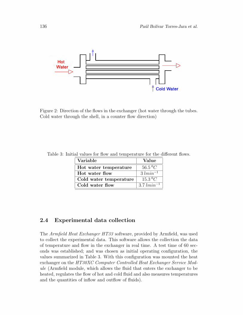
The flow and temperature variables were established for two types of flow: hotwater and cold water; following the direction of the flow, as shown in Figure2. The initial values for these variables are presented in Table 3.


Figure 2: Direction of the flows in the exchanger (hot water through the tubes.Cold water through the shell, in a counter flow direction)

Table 3: Initial values for flow and temperature for the different flows.

Variable Value

Hot water temperature 56.5 0CHot water flow 3 lmin−1

Cold water temperature 15.3 0CCold water flow 3.7 lmin−1

2.4 Experimental data collection

The Armfield Heat Exchanger HT33 software, provided by Armfield, was usedto collect the experimental data. This software allows the collection the dataof temperature and flow in the exchanger in real time. A test time of 60 sec-onds was established; and was chosen as initial operating configuration, thevalues summarized in Table 3. With this configuration was mounted the heatexchanger on the HT30XC Computer Controlled Heat Exchanger Service Mod-ule (Armfield module, which allows the fluid that enters the exchanger to beheated, regulates the flow of hot and cold fluid and also measures temperaturesand the quantities of inflow and outflow of fluids).


2.5 Simulation

The SolidWorks2 software was used to simulate the heat exchange processesthat take place in the device. First the three-dimensional design of the heatexchanger was obtained and then the computer simulation of heat transferwas carried out. Figure 3 shows the three-dimensional representation of theequipment.

Figure 3: Three-dimensional design of the Shell and Tube Exchanger

2.5.1 Simulation parameters

The parameters that were used into the simulation software, were the flowvalues obtained through the real time measurement, are shown in Table 4.Three types of mesh quality were used for the simulation. The software allowsautomatically generate the “thick”, “medium” and “fine” mesh types. Thecharacteristics of each type of mesh are shown in Table 5.

2The SolidWorks software was used under license provided by Universidade EstadualPualista “Julio de Mesquita Filho”. Garantingueta, Brasil.


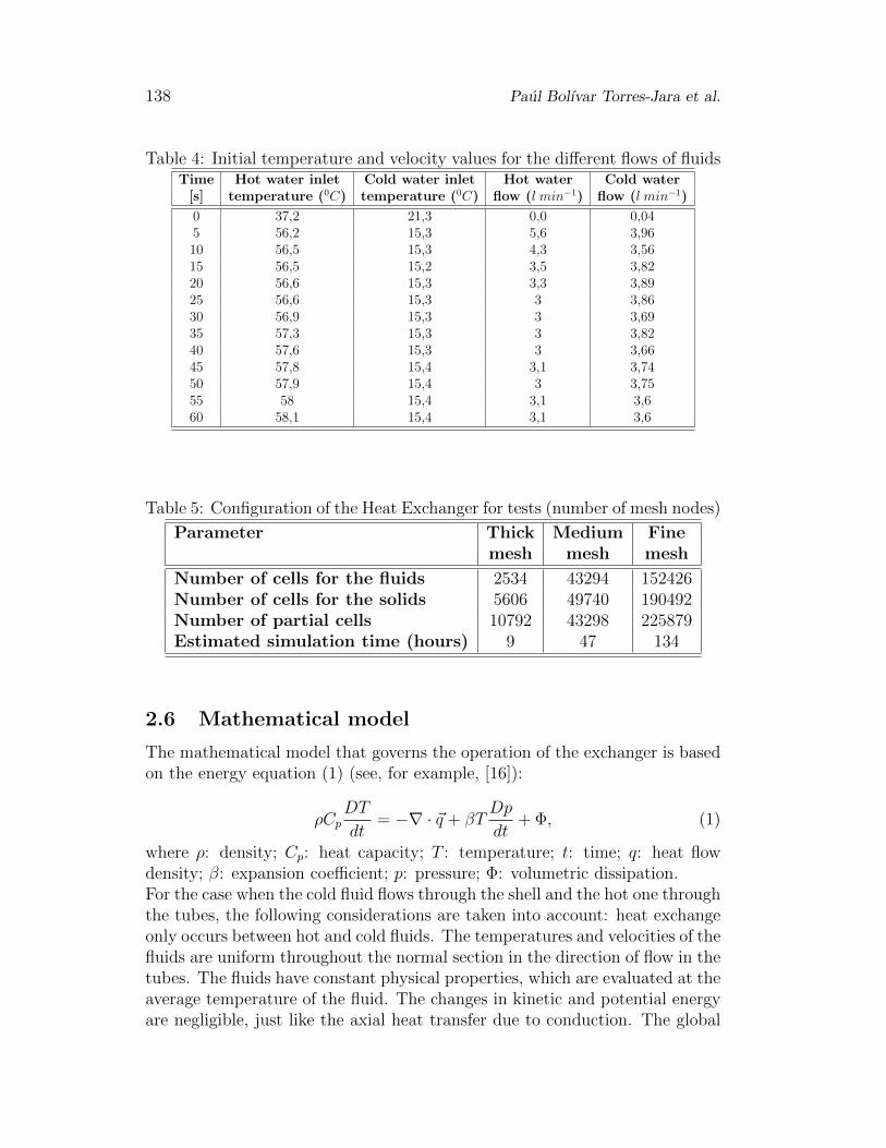
Table 4: Initial temperature and velocity values for the different flows of fluidsTime Hot water inlet Cold water inlet Hot water Cold water

[s] temperature (0C) temperature (0C) flow (l min−1) flow (l min−1)

0 37,2 21,3 0,0 0,045 56,2 15,3 5,6 3,9610 56,5 15,3 4,3 3,5615 56,5 15,2 3,5 3,8220 56,6 15,3 3,3 3,8925 56,6 15,3 3 3,8630 56,9 15,3 3 3,6935 57,3 15,3 3 3,8240 57,6 15,3 3 3,6645 57,8 15,4 3,1 3,7450 57,9 15,4 3 3,7555 58 15,4 3,1 3,660 58,1 15,4 3,1 3,6

Table 5: Configuration of the Heat Exchanger for tests (number of mesh nodes)

Parameter Thick Medium Finemesh mesh mesh

Number of cells for the fluids 2534 43294 152426Number of cells for the solids 5606 49740 190492Number of partial cells 10792 43298 225879Estimated simulation time (hours) 9 47 134

2.6 Mathematical model

The mathematical model that governs the operation of the exchanger is basedon the energy equation (1) (see, for example, [16]):

ρCpDT

dt= −∇ · ~q + βT

Dp

dt+ Φ, (1)

where ρ: density; Cp: heat capacity; T : temperature; t: time; q: heat flowdensity; β: expansion coefficient; p: pressure; Φ: volumetric dissipation.For the case when the cold fluid flows through the shell and the hot one throughthe tubes, the following considerations are taken into account: heat exchangeonly occurs between hot and cold fluids. The temperatures and velocities of thefluids are uniform throughout the normal section in the direction of flow in thetubes. The fluids have constant physical properties, which are evaluated at theaverage temperature of the fluid. The changes in kinetic and potential energyare negligible, just like the axial heat transfer due to conduction. The global


coefficient of heat transfer is constant. The mass flow is constant throughthe tubes and shell. There is no change in the pressure drop in the system.There is no phase change of the fluids. The transitions through the exchangeroccur by horizontal and vertical sections. The idealizations considered allowobtaining, from equation (1), equations (2) and (3) that describe the dynamicbehavior of each part of the system:

mtCpt

(T it − T o

t

)+ FUA (Ts − Tt) = ρtCptVt

Ttdt, (2)

msCps

(T is − T o

s

)+ FUA (Ts − Tt) = ρsCpsVs

Tsdt, (3)

where the subscript t refers to the tubes and the subscript s to the shell.Besides, T i: inlet temperatures of the fluids; T o: outlet temperatures of thefluids; F : correction factor; U : global coefficient of heat transfer; A: heattransfer area; V : fluid volume.

3 Results

3.1 Experimental

Table 6 shows the experimental results obtained by measuring outlet temper-atures (for both hot and cold water), taken at 5-second intervals. As can beseen in this table, the values tend to stabilize after 20 seconds.

Table 6: Experimental outlet temperatures

Time Hot water outlet Cold water outlet[s] temperature (0C) temperature (0C)

0 35,8 18,15 51,8 22,110 51 20,815 51 20,320 50,5 19,925 50,5 19,830 50,7 19,735 51,6 19,840 51,3 19,845 51,3 19,850 51,4 19,955 51,6 19,860 51,5 19,9


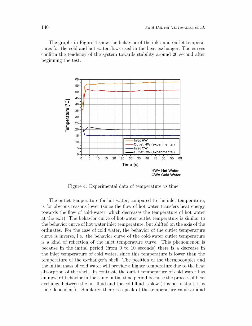
The graphs in Figure 4 show the behavior of the inlet and outlet tempera-tures for the cold and hot water flows used in the heat exchanger. The curvesconfirm the tendency of the system towards stability around 20 second afterbeginning the test.

Figure 4: Experimental data of temperature vs time

The outlet temperature for hot water, compared to the inlet temperature,is for obvious reasons lower (since the flow of hot water transfers heat energytowards the flow of cold-water, which decreases the temperature of hot waterat the exit). The behavior curve of hot-water outlet temperature is similar tothe behavior curve of hot water inlet temperature, but shifted on the axis of theordinates. For the case of cold water, the behavior of the outlet temperaturecurve is inverse, i.e. the behavior curve of the cold-water outlet temperatureis a kind of reflection of the inlet temperature curve. This phenomenon isbecause in the initial period (from 0 to 10 seconds) there is a decrease inthe inlet temperature of cold water, since this temperature is lower than thetemperature of the exchanger’s shell. The position of the thermocouples andthe initial mass of cold water will provide a higher temperature due to the heatabsorption of the shell. In contrast, the outlet temperature of cold water hasan upward behavior in the same initial time period because the process of heatexchange between the hot fluid and the cold fluid is slow (it is not instant, it istime dependent) . Similarly, there is a peak of the temperature value around


5 seconds, caused by the thermal inertia of the fluid, that is, the opposition tochange the state. In this case, changing from one state of heat absorption, toone of stable temperature.

3.2 Computational

Table 7 shows the simulated results of outlet temperature of hot water forthick, medium and fine mesh. As shown, the temperature values are stabilizedat a time, which is similar to the experimental stabilization time. Additionally,the type of mesh does not have a significant influence on the simulation results.However, a better quality of the mesh (finer) will produce results more close upto the experimental ones. Moreover, there is a peak in the outlet temperatureof hot water around 2 seconds, due to the thermal inertia considered by thesoftware.

Table 7: Simulation results (output temperatures, hot water)

Time Thick Medium Fine[s] mesh mesh mesh

0 18,05 18,05 18,055 52,08 53,08 52,6310 51,78 52,38 52,615 51,51 52,11 52,5520 51,57 52,09 52,5325 51,59 52,07 52,5130 51,58 52,05 52,5035 51,58 51,98 52,4940 51,58 51,98 52,4945 51,58 51,98 52,4950 51,58 51,98 52,4955 51,58 51,98 52,4960 51,58 51,98 52,49

Table 8 shows the results obtained for the outlet temperature of cold waterand the same types of meshing. We can see a behavior that is similar to theprevious case, now the temperature values with medium and fine mesh arecloser to the values obtained experimentally. Similarly, at the beginning of theprocess, the values obtained with those meshes, show a similar behavior to theone demonstrated experimentally. Not so for the thick mesh.


Table 8: Simulation results (output temperatures, cold-water)

Time Thick Medium Fine[s] mesh mesh mesh

0 18,05 18,05 18,055 19,39 19,68 19,8610 19,29 19,53 19,7815 19,18 19,51 19,7520 19,18 19,49 19,7425 19,18 19,47 19,7330 19,18 19,47 19,7135 19,18 19,47 19,7140 19,18 19,47 19,7145 19,18 19,47 19,7150 19,18 19,47 19,7155 19,18 19,47 19,7160 19,18 19,47 19,71

The heat transfer process is shown in Figure 5 that appears later, whichshows how the temperature varies according to time. The transverse sectionscorrespond to the location of cold-water inflow and outflow; the images wereobtained from the data with fine mesh. In the first section, in the bottom partwhere there is inflow of cold water, the temperature of hot water is not the samein all the tubes of the exchanger. This is due to the position of the fluid inletpoint, which, when displaced downwards, will lose heat as it moves farther untilit reaches the upper tubes. As time progresses, a difference in temperature canbe seen in each of the tubes. That is, a lower fluid temperature at the bottomof each tube, due to the position of the cold-water inlet, since the first contactsurface is the bottom of each tube. At the height of the twelfth, it is nowpossible to see, thanks to changes in color tone, how the heat transfer causedby the temperature gradient occurs. It is also possible to see that as timeprogresses; temperatures stabilize, and acquire a more homogenous tone. Inaddition, it is possible to appreciate the points where there is greater transferof heat between the walls of the tubes and the fluid.


Time[s] Cold water intake Cold water outlet

0

2

4

6

8

10

56, 5 0C 15, 5 0C

Figure 5: Simulated behavior of inlet and outlet temperatures of cold-water

3.3 Comparison of results

The comparison between the experimental and simulated results allows thevalidation of the computational tool, that is, it describes the processes thatoccur in the heat exchanger with a good level of accuracy. The graph of Figure


6 shows the hot water, experimental and simulated temperature curves withthe different types of mesh. It is possible to appreciate the similarity betweenthem, as well as for the equilibrium values. The variations observed in theexperimental curve are attributable to several factors, such as the accuracy ofmeasuring instruments, heat losses in pipes and fittings, impurities in the fluidand the inertia of the fluid that resists a status change. After 50 seconds, theequilibrium values are similar.

Figure 6: Behavior curves for outlet temperatures, hot water (simulated andexperimental)

The comparison of results for the cold-water outlet temperature curves isshown in Figure 7. In this case, there is also a similarity between them, and thetemperature equilibrium values are similar with a tolerance of ±0, 5 0C. Forthe experimental curve, the temperature increase occurs a few seconds laterthan for the simulated ones. Once again, the factor that influences that mostis the thermal inertia of the fluid. As in the case of hot water, it is possibleto see the effect of better meshing, especially at the beginning of the process.At the beginning of the process, the experimental curve has a peak at about 5seconds, as opposed to the simulated curves. This behavior is explained by thecharacteristics of a heat transfer process, for which the temperature requiressome time to stabilize.


Figure 7: Behavior curves for outlet temperatures, cold water (simulated andexperimental)

In general, both the experimental and the simulated results have similarbehaviors and stabilize at similar times. The maximum percentage of relativeerror between the experimental and computational data of the exit tempera-ture for hot water, if analyzed from the moment of stabilization of the process(20 seconds after it started), is approximately 4%, and is obtained for the finemesh. While the same error for the cold-water outlet temperature is approxi-mately 3, 62% for the thick meshing.

4 Conclusions

The outlet temperature curves for hot and cold water have similar tendenciesfor the experimental and the simulated data, therefore is validated the com-putational tool used to simulate the operation of the exchanger. The valuesobtained are coherent with the tolerances recorded in previous research. Forexample, in [8] with a numerical solution of the mathematical model that de-scribes the operation of the exchanger, under certain conditions a tolerance of10% is reached; however, the maximum relative error in the simulation pro-posed in this work, also under certain conditions (temporary in this case), doesnot exceed 5%. The result obtained is also comparable, in terms of deviation,with that obtained by the authors in [7]. Therefore, when there is any situationthat hinders the use of the heat exchanger in the thermo-fluids laboratory, it ispossible to continue the laboratory practices and the normal course of lessonsby applying the simulation. Additionally, the simulation technique becomesan educational tool to predict behaviors of the temperature curves in the ex-changer when the conditions or initial data go beyond the established rangesfor the laboratory exchanger.


References

[1] Y. You, Y. Chen, M. Xi, X. Luo, L. Jiao, S. Huang, Numerical simula-tion and performance improvement for a small size shell-and-tube heat ex-changer with trefoil-hole baffles, Applied Thermal Engineering, 89 (2015),220 – 228. https://doi.org/10.1016/j.applthermaleng.2015.06.012

[2] R. Curtain, Structural theory of distributed systems, Acta ApplicandaeMathematica, 2 (1984), no. 2, 209–210.https://doi.org/10.1023/a:1010642900190

[3] M. Prithiviraj, M. Andrews, Three-dimensional numerical simulation ofshell-and-tube heat exchangers. Part I: foundation and fluid mechanics,Numerical Heat Transfer, Part A. Applications, 33 (1998), no. 8, 799–816.https://doi.org/10.1080/10407789808913967

[4] M. B. Reyes-Rodrıguez, J. L. Moya-Rodrıguez, O. M. Cruz-Fonticiella,E. M. Fırvida-Donestevez, J. A. Velazquez-Perez, Automatizacion y opti-mizacion del diseno de intercambiadores de calor de tubo y coraza medianteel metodo de Taborek, Revista Ingenierıa Mecanica, 17 (2014), no. 1.

[5] M. Hatami, M. Boot, D. Ganji, M. Bandpy, Comparative study of differ-ent exhaust heat exchangers effect on the performance and exergy analy-sis of a diesel engine, Applied Thermal Engineering, 90 (2015), 23 – 37.https://doi.org/10.1016/j.applthermaleng.2015.06.084

[6] M. Ardila, Z. Hincapie, M. Casas, Validacion de modelos numericos du-rante el desarrollo de correlaciones para intercambiadores de calor, Actasde Ingenierıa, 1 (2015), 164-168.

[7] D. Correa, J. Marchetti, Dynamic Simulation of Shell-and-Tube Heat Ex-changers, Heat Transfer Engineering, 8 (1987), no. 1, 50–59.https://doi.org/10.1080/01457638708962787

[8] G. Nellis, A heat exchanger model that includes axial conduction, parasiticheat loads, and property variations, Cryogenics, 43 (2003), no. 9, 523 – 538.https://doi.org/10.1016/s0011-2275(03)00132-2

[9] A. Kanaris, A. Mouza, S. Paras, Flow and Heat Transfer Prediction in aCorrugated Plate Heat Exchanger using a CFD Code, Chemical Engineer-ing & Technology, 29 (2006), no. 8, 923–930.https://doi.org/10.1002/ceat.200600093

[10] J. Judge, R. Radermacher, A heat exchanger model for mixtures andpure refrigerant cycle simulations, International Journal of Refrigeration,


20 (1997), no. 4, 244 – 255. https://doi.org/10.1016/s0140-7007(97)00010-8

[11] E. Cordova-Tuta, D. Fuentes-Dıaz, Modeling and simulation of flow in fin-and-tube heat exchangers with phase change in the coolant side, RevistaInternacional de Metodos Numericos para Calculo y Diseno en Ingenierıa,32 (2016), no. 1, 31-38. https://doi.org/10.1016/j.rimni.2014.11.002

[12] J. Ricardo-Barrera, E. Barrios-Uruena, Control multivariable lineal condesacoples en un intercambiador de calor, Revista Ingenierıa, Investigaciony Desarrollo, 17 (2017), no. 1, 17-25.

[13] A. Trp, An experimental and numerical investigation of heat transfer dur-ing technical grade paraffin melting and solidification in a shell-and-tubelatent thermal energy storage unit, Solar Energy, 79 (2005), no. 6, 648 –660. https://doi.org/10.1016/j.solener.2005.03.006

[14] F. Machuca, O. Urresta, Software para la ensenanza de la dinamica ycontrol de intercambiadores de calor de tubos y coraza, Revista Facultadde Ingenierıa, Universidad de Antioquia, (2008), no. 44, 52-60.

[15] M. B. Reyes-Rodrıguez, J. L. Moya-Rodrıguez, Design and Optimizationof Shell and tube exchangers, state of the art, Journal of Engineering andTechnology for Industrial Applications (ITEGAM-JETIA), 2 (2016), no. 6,4-27. https://doi.org/10.5935/2447-0228.20160011

[16] C. N. Ranong, W. Roetzel, Steady-state and transient behaviour of twoheat exchangers coupled by a circulating flowstream, International Journalof Thermal Sciences, 41 (2002), no. 11, 1029-1043.https://doi.org/10.1016/S1290-0729(02)01390-X

Received: June 19, 2019; Published: July 12, 2019

Documents

Operation of a Shell and Tubes Heat Exchanger: …...Operation of a shell and tubes heat exchanger 137 2.5 Simulation The SolidWorks2 software was used to simulate the heat exchange