On The Relations between SINR Diagrams andVoronoi Diagrams

Merav Parter and David Peleg

The Weizmann Institute of Science, Rehovot, Israel.merav.parter,david.peleg@ weizmann.ac.il ?

Abstract. In this review, we illustrate the relations between wirelesscommunication and computational geometry. As a concrete example, weconsider a fundamental geometric object from each field: SINR diagramsand Voronoi diagrams. We discuss the relations between these represen-tations, which appear in several distinct settings of wireless communica-tion, as well as some algorithmic applications.

1 Introduction

Wireless networks are embedded in our daily lives, with an ever-growing useof cellular, satellite and sensor networks. Subsequently, the capacity of wirelessnetworks, i.e., the maximum achievable rate by which stations can communicatereliably, has received an increasing attention in recent years [15, 20, 18, 14, 7,2, 16]. The great advantage of wireless communication, namely, the broadcastnature of the medium, also creates its biggest obstacle – interference. Whena receiver has to decode a message (i.e., a signal) sent from a transmitter, itmust cope with all other (legitimate) simultaneous transmissions by neighboringstations.

While the physical properties of channels have been thoroughly studied [13,22], less is known about the topology and geometry of the wireless network struc-ture and their influence on performance. This review concerns a novel approachrecently proposed to describe the behavior of multi-station networks, which isbased on building a reception map according to the signal-to-interference &noise ratio (SINR) model. By now, the SINR model is the most commonly stud-ied abstract physical model for wireless communication networks, widely usedby both the Electrical Engineering community and the algorithmic computerscience community. This physical model aims at gauging the quality of signalreception at the receivers while faithfully representing phenomena such as atten-uation and interference. Specifically, in this model, the signal decays as it travelsand a transmission is successful if its strength at the receiver exceeds the accu-mulated signal strength of interfering transmissions by a sufficient (technologydetermined) factor.

? Supported in part by the Israel Science Foundation (grant 894/09) and the IsraelMinistry of Science and Technology (infrastructures grant).

𝐻(𝑠1)

𝐻(𝑠2) 𝐻(𝑠3)

𝐻(𝑠4)

𝑆𝐼𝑁𝑅 Diagram

𝐻(∅)

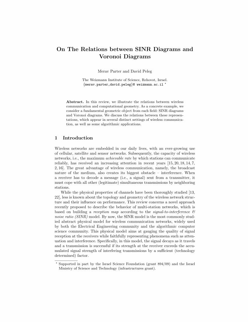
The SINR model gives rise to a natural ge-ometric object, the SINR diagram, which par-titions the plane into a reception region H(si)per station si ∈ S and the remaining areaH(∅) where none of the stations are heard.Each of these n + 1 regions may possibly becomposed of several disconnected regions.

SINR diagrams have been recently studiedfrom topological and geometric standpoints[6, 17, 5], and they appear to provide improvedunderstanding on the behavior of wireless net-works. Specifically, these diagram have beenshown to play a central role in the devel-opment of several approximation and onlinealgorithms (e.g., point location tasks, mapdrawing). Such a role is analogous perhaps to the role played by Voronoi di-agrams in the study of proximity queries and other algorithms in computationalgeometry.

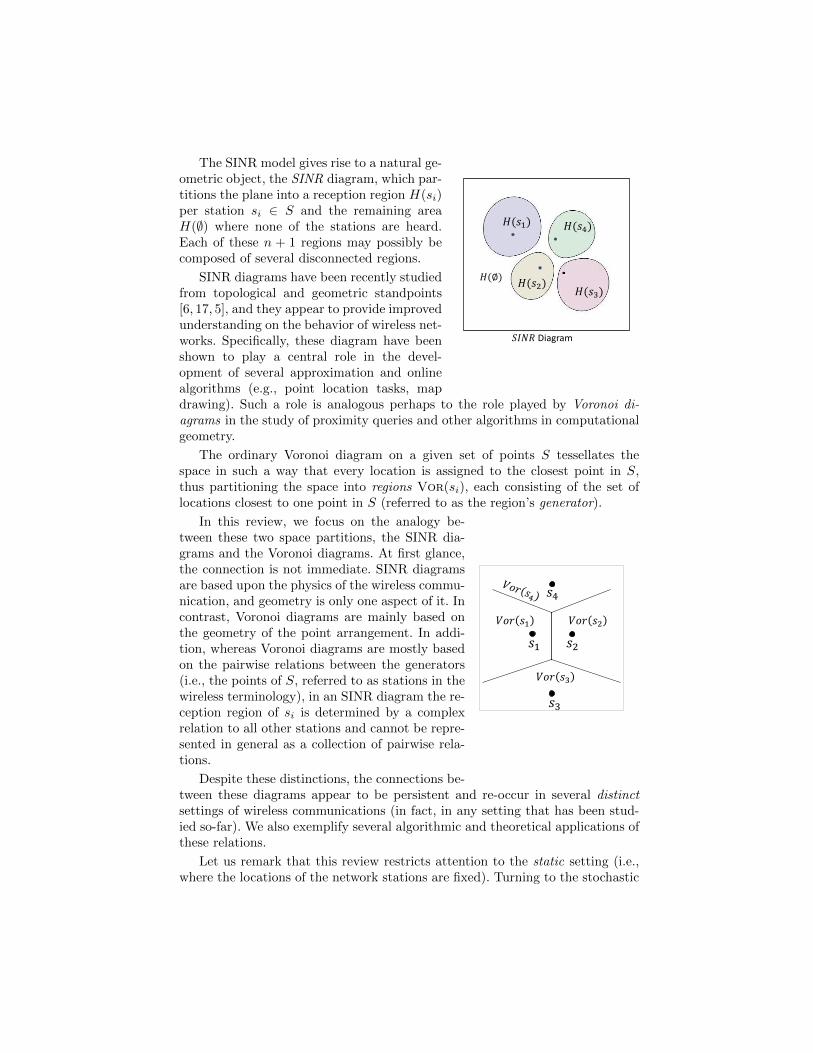
The ordinary Voronoi diagram on a given set of points S tessellates thespace in such a way that every location is assigned to the closest point in S,thus partitioning the space into regions Vor(si), each consisting of the set oflocations closest to one point in S (referred to as the region’s generator).

𝑠3

𝑠2 𝑠1

𝑠4

𝑉𝑜𝑟 𝑠2

𝑉𝑜𝑟 𝑠3

𝑉𝑜𝑟 𝑠1

In this review, we focus on the analogy be-tween these two space partitions, the SINR dia-grams and the Voronoi diagrams. At first glance,the connection is not immediate. SINR diagramsare based upon the physics of the wireless commu-nication, and geometry is only one aspect of it. Incontrast, Voronoi diagrams are mainly based onthe geometry of the point arrangement. In addi-tion, whereas Voronoi diagrams are mostly basedon the pairwise relations between the generators(i.e., the points of S, referred to as stations in thewireless terminology), in an SINR diagram the re-ception region of si is determined by a complexrelation to all other stations and cannot be repre-sented in general as a collection of pairwise rela-tions.

Despite these distinctions, the connections be-tween these diagrams appear to be persistent and re-occur in several distinctsettings of wireless communications (in fact, in any setting that has been stud-ied so-far). We also exemplify several algorithmic and theoretical applications ofthese relations.

Let us remark that this review restricts attention to the static setting (i.e.,where the locations of the network stations are fixed). Turning to the stochastic

setting, the relations between stochastic SINR diagram (formed by modeling theSINR as a marked point process) and classical stochastic geometry models suchas PoissonVoronoi tessellations, have been studied extensively, and are out ofthe scope of this review. See [8] for a detailed analysis, results and applicationsof this approach.

The structure of this review is as follows. In Sec. 2 we provide a brief overviewof SINR diagrams. We then describe the connections between SINR diagrams andVoronoi diagrams in three main settings. Sec. 3 considers the uniform power set-ting, when all stations have the same transmission power. In Sec. 4, we considerthe general setting of non-uniform power (i.e., when the transmission powers arearbitrary). Finally, in Sec. 5, we describe a setting in which receivers are allowedto employ a decoding technique known as interference cancellation to improvetheir reception quality. In each of these settings, the resulting SINR diagramsturn out to correspond to some variant of Voronoi diagrams, as elaborated onin what follows.

2 Wireless Networks and SINR

We consider a wireless network A = 〈d, S, ψ,N , β, α〉, where d ∈ Z≥1 is thedimension, S = s1, s2, . . . , sn is a set of transmitting radio stations embeddedin the d-dimensional space, ψ is an assignment of a positive real transmittingpower ψi to each station si, N ≥ 0 is the background noise, β ≥ 1 is a constantthat serves as the reception threshold, and α > 0 is the path-loss parameter. Thesignal to interference & noise ratio (SINR) of si at point p is defined as

SINRA(si, p) =ψi · dist(si, p)

−α∑j 6=i ψj · dist(sj , p)−α + N

. (1)

The fundamental rule of the SINR model is that the transmission of stationsi is received correctly at point p /∈ S if and only if its SINR at p reaches orexceeds the reception threshold of the network, i.e., SINRA(si, p) ≥ β. Whenthis happens, we say that si is heard at p.

We refer to the set of points that hear station si as the reception region ofsi, defined as

H(si,A) = p ∈ Rd − S | SINRA(si, p) ≥ β ∪ si . (2)

(Note that SINR(si, ·) is undefined at points in S and in particular at si itself.)Analogously, the set of points that hear no station si ∈ S (due to the backgroundnoise and interference), the null region, is defined as

H(∅,A) = p ∈ Rd − S | SINR(si, p) < β, ∀si ∈ S.

An SINR diagram

H(A) =

( ⋃si∈S

H(si,A)

)∪H(∅,A)

is a “reception map” characterizing the reception regions of the stations. Whenthe network A is clear from the context, we may omit it, and simply writeSINR(si, p), H(si) and H(∅).

3 Uniform SINR Diagram and Voronoi Diagram

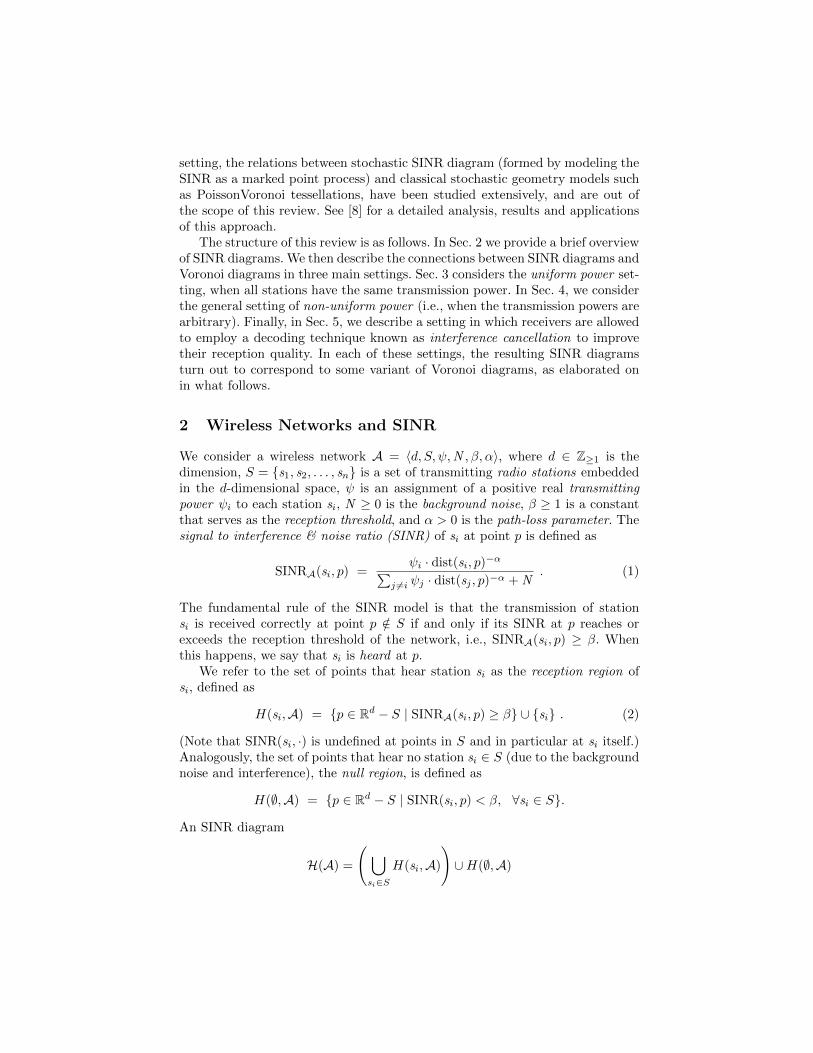
The study of SINR diagram has been initiated by Avin et al. in [6] for therelatively simple case where all stations use the same transmission power, a.k.a,uniform power (i.e., ψi = 1 for every station si in Eq. (1)). It has been shownthat under this setting, the SINR diagram assumes a rather convenient form. Inparticular, for SINR threshold β ≥ 1, it holds that every reception region H(si)is convex and fat (see Fig. 1(a) for schematic illustration of these notions).

(a) (b)

Fig. 1. (a) Uniform SINR regions are “nice”: convex and fat. (b) Illustration of therelations between uniform SINR diagram and Voronoi diagram. The reception regionH(si) is fully contained in the corresponding Voronoi region Vor(si).

Let Vor(si) be the Voronoi region of station si, defined by

Vor(si) = p ∈ Rd | dist(si, p) ≤ dist(sj , p), , for any j 6= i . (3)

Since all transmission powers are the same, for a receiver p that successfullyreceives the transmission of si, it must hold that si is the closest station top among all other network stations, i.e., that p ∈ Vor(si). This condition isnot sufficient for successful reception, and hence uniform SINR diagrams can beconsidered as a refinement of Voronoi diagrams. The refinement stems from thatfact that the SINR model (even in the uniform case) takes into considerationnot only the geometry but also other physical parameters such as attenuationand fading of signals.

The following lemma from [6] formalizes this intuition by claiming that thereception region H(si,A) is strictly contained in the corresponding Voronoi re-gion Vor(si).

Lemma 1 (Uniform SINR Diagram and Voronoi Diagram, [6]). Foruniform network A = 〈d, S, 1,N , β ≥ 1, α〉, it holds that H(si,A) ⊆ Vor(si) forevery si ∈ S.

See Fig. 1(b). In fact, this analogy between the two diagrams becomes strongerwhen the path-loss parameter α tends to infinity and there is no ambient noiseN = 0. The case of noisy SINR diagram with α→∞ and N > 0 is more involvedand can be shown to converge to alpha shapes [11].

Note that when β < 1, the inclusion between the SINR diagram and theVoronoi diagram may no longer hold. That is, it is possible to identify pointsp ∈ Rd, for which SINR(si, p) ≥ β while p /∈ Vor(si).

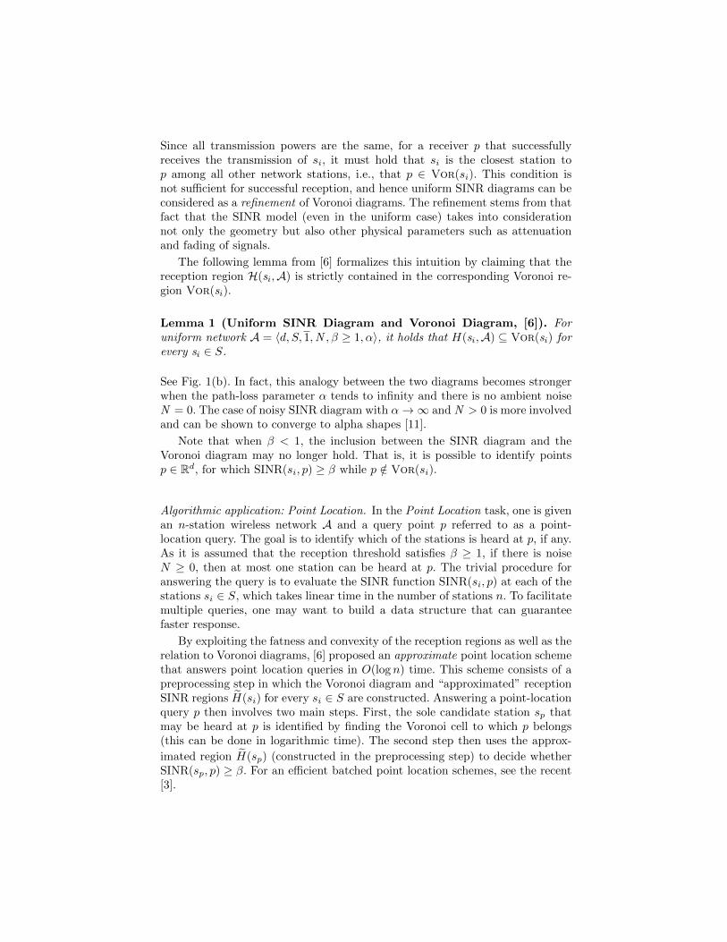
Algorithmic application: Point Location. In the Point Location task, one is givenan n-station wireless network A and a query point p referred to as a point-location query. The goal is to identify which of the stations is heard at p, if any.As it is assumed that the reception threshold satisfies β ≥ 1, if there is noiseN ≥ 0, then at most one station can be heard at p. The trivial procedure foranswering the query is to evaluate the SINR function SINR(si, p) at each of thestations si ∈ S, which takes linear time in the number of stations n. To facilitatemultiple queries, one may want to build a data structure that can guaranteefaster response.

By exploiting the fatness and convexity of the reception regions as well as therelation to Voronoi diagrams, [6] proposed an approximate point location schemethat answers point location queries in O(log n) time. This scheme consists of apreprocessing step in which the Voronoi diagram and “approximated” receptionSINR regions H(si) for every si ∈ S are constructed. Answering a point-locationquery p then involves two main steps. First, the sole candidate station sp thatmay be heard at p is identified by finding the Voronoi cell to which p belongs(this can be done in logarithmic time). The second step then uses the approx-

imated region H(sp) (constructed in the preprocessing step) to decide whetherSINR(sp, p) ≥ β. For an efficient batched point location schemes, see the recent[3].

4 Non-uniform SINR Diagram and Weighted VoronoiDiagram

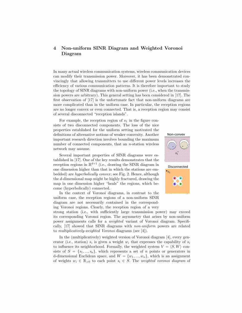
In many actual wireless communication systems, wireless communication devicescan modify their transmission power. Moreover, it has been demonstrated con-vincingly that allowing transmitters to use different power levels increases theefficiency of various communication patterns. It is therefore important to studythe topology of SINR diagrams with non-uniform power (i.e., when the transmis-sion powers are arbitrary). This general setting has been considered in [17]. Thefirst observation of [17] is the unfortunate fact that non-uniform diagrams aremore complicated than in the uniform case. In particular, the reception regionsare no longer convex or even connected. That is, a reception region may consistof several disconnected “reception islands”.

Non-convex

Disconnected

𝑠1

𝑠1

For example, the reception region of s1 in the figure con-sists of two disconnected components. The loss of the niceproperties established for the uniform setting motivated thedefinitions of alternative notions of weaker convexity. Anotherimportant research direction involves bounding the maximumnumber of connected components, that an n-station wirelessnetwork may assume.

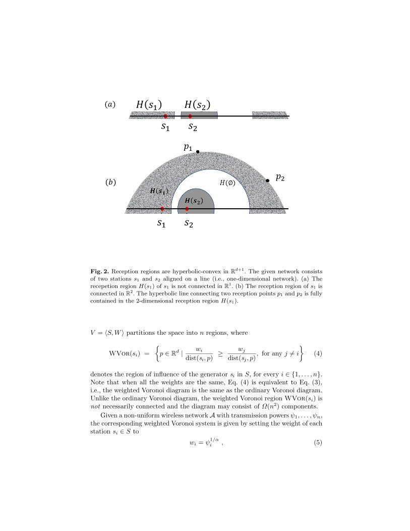
Several important properties of SINR diagrams were es-tablished in [17]. One of the key results demonstrates that thereception regions in Rd+1 (i.e., drawing the SINR diagram inone dimension higher than that in which the stations are em-bedded) are hyperbolically convex ; see Fig. 2. Hence, althoughthe d-dimensional map might be highly fractured, drawing themap in one dimension higher “heals” the regions, which be-come (hyperbolically) connected.

In the context of Voronoi diagrams, in contrast to theuniform case, the reception regions of a non-uniform SINRdiagram are not necessarily contained in the correspond-ing Voronoi regions. Clearly, the reception region of a verystrong station (i.e., with sufficiently large transmission power) may exceedits corresponding Voronoi region. The asymmetry that arises by non-uniformpower assignments calls for a weighted variant of Voronoi diagram. Specifi-cally, [17] showed that SINR diagrams with non-uniform powers are relatedto multiplicatively-weighted Voronoi diagrams (see [4]).

In the (multiplicatively) weighted version of Voronoi diagram [4], every gen-erator (i.e., station) si is given a weight wi that expresses the capability of sito influence its neighborhood. Formally, the weighted system V = 〈S,W 〉 con-sists of S = s1, ..., sn, which represents a set of n points or generators ind-dimensional Euclidean space, and W = w1, ..., wn, which is an assignmentof weights wi ∈ R>0 to each point si ∈ S. The weighted voronoi diagram of

𝑠1 𝑠2

𝐻 𝑠1 𝐻 𝑠2

𝑠1 𝑠2

𝑝1

𝑝2 (𝑏)

(𝑎)

Fig. 2. Reception regions are hyperbolic-convex in Rd+1. The given network consistsof two stations s1 and s2 aligned on a line (i.e., one-dimensional network). (a) Therecepetion region H(s1) of s1 is not connected in R1. (b) The reception region of s1 isconnected in R2. The hyperbolic line connecting two reception points p1 and p2 is fullycontained in the 2-dimensional reception region H(s1).

V = 〈S,W 〉 partitions the space into n regions, where

WVor(si) =

p ∈ Rd | wi

dist(si, p)≥ wj

dist(sj , p), for any j 6= i

(4)

denotes the region of influence of the generator si in S, for every i ∈ 1, . . . , n.Note that when all the weights are the same, Eq. (4) is equivalent to Eq. (3),i.e., the weighted Voronoi diagram is the same as the ordinary Voronoi diagram.Unlike the ordinary Voronoi diagram, the weighted Voronoi region WVor(si) isnot necessarily connected and the diagram may consist of Ω(n2) components.

Given a non-uniform wireless networkA with transmission powers ψ1, . . . , ψn,the corresponding weighted Voronoi system is given by setting the weight of eachstation si ∈ S to

wi = ψ1/αi , (5)

where α is the path-loss parameter of the wireless network. This weight ad-justment yields the next lemma, the analogue of Lemma 2 for the non-uniformcase.

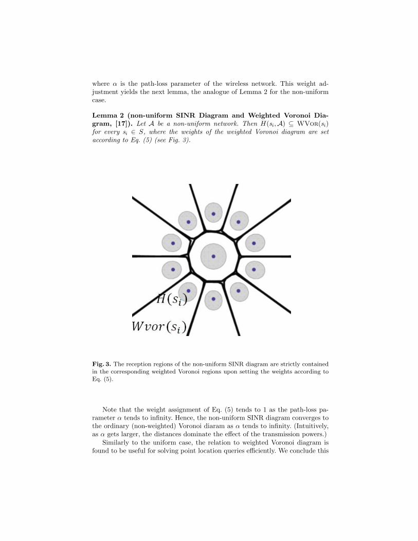
Lemma 2 (non-uniform SINR Diagram and Weighted Voronoi Dia-gram, [17]). Let A be a non-uniform network. Then H(si,A) ⊆ WVor(si)for every si ∈ S, where the weights of the weighted Voronoi diagram are setaccording to Eq. (5) (see Fig. 3).

Fig. 3. The reception regions of the non-uniform SINR diagram are strictly containedin the corresponding weighted Voronoi regions upon setting the weights according toEq. (5).

Note that the weight assignment of Eq. (5) tends to 1 as the path-loss pa-rameter α tends to infinity. Hence, the non-uniform SINR diagram converges tothe ordinary (non-weighted) Voronoi diaram as α tends to infinity. (Intuitively,as α gets larger, the distances dominate the effect of the transmission powers.)

Similarly to the uniform case, the relation to weighted Voronoi diagram isfound to be useful for solving point location queries efficiently. We conclude this

section by providing an example in which weighted Voronoi diagrams are nothelpful, due to some fundamental differences between the two models.

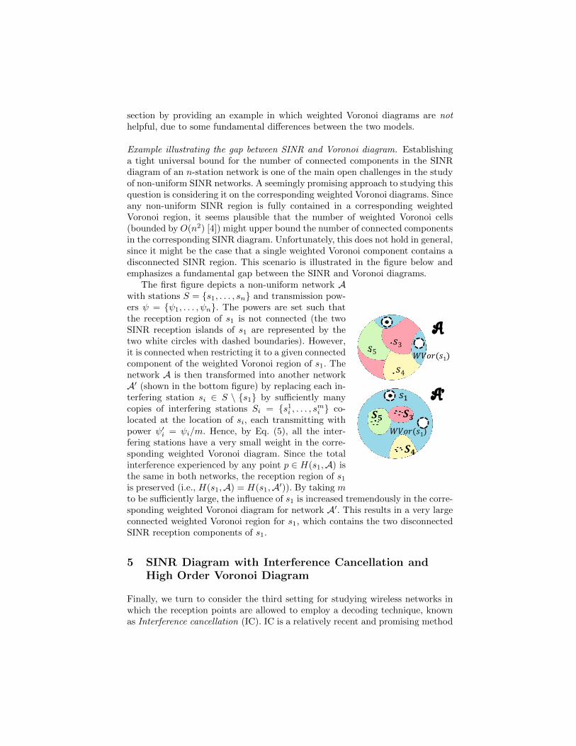
Example illustrating the gap between SINR and Voronoi diagram. Establishinga tight universal bound for the number of connected components in the SINRdiagram of an n-station network is one of the main open challenges in the studyof non-uniform SINR networks. A seemingly promising approach to studying thisquestion is considering it on the corresponding weighted Voronoi diagrams. Sinceany non-uniform SINR region is fully contained in a corresponding weightedVoronoi region, it seems plausible that the number of weighted Voronoi cells(bounded by O(n2) [4]) might upper bound the number of connected componentsin the corresponding SINR diagram. Unfortunately, this does not hold in general,since it might be the case that a single weighted Voronoi component contains adisconnected SINR region. This scenario is illustrated in the figure below andemphasizes a fundamental gap between the SINR and Voronoi diagrams.

𝑠1

𝑠3

𝑠4

𝑠5 𝑊𝑉𝑜𝑟(𝑠1)

A

𝑺𝟑

𝑠1

𝑺𝟒

𝑺𝟓

A’

𝑊𝑉𝑜𝑟(𝑠1)

The first figure depicts a non-uniform network Awith stations S = s1, . . . , sn and transmission pow-ers ψ = ψ1, . . . , ψn. The powers are set such thatthe reception region of s1 is not connected (the twoSINR reception islands of s1 are represented by thetwo white circles with dashed boundaries). However,it is connected when restricting it to a given connectedcomponent of the weighted Voronoi region of s1. Thenetwork A is then transformed into another networkA′ (shown in the bottom figure) by replacing each in-terfering station si ∈ S \ s1 by sufficiently manycopies of interfering stations Si = s1i , . . . , smi co-located at the location of si, each transmitting withpower ψ′i = ψi/m. Hence, by Eq. (5), all the inter-fering stations have a very small weight in the corre-sponding weighted Voronoi diagram. Since the totalinterference experienced by any point p ∈ H(s1,A) isthe same in both networks, the reception region of s1is preserved (i.e., H(s1,A) = H(s1,A′)). By taking mto be sufficiently large, the influence of s1 is increased tremendously in the corre-sponding weighted Voronoi diagram for network A′. This results in a very largeconnected weighted Voronoi region for s1, which contains the two disconnectedSINR reception components of s1.

5 SINR Diagram with Interference Cancellation andHigh Order Voronoi Diagram

Finally, we turn to consider the third setting for studying wireless networks inwhich the reception points are allowed to employ a decoding technique, knownas Interference cancellation (IC). IC is a relatively recent and promising method

for efficient decoding [1]. The basic idea of interference cancellation, and inparticular successive interference cancellation (SIC), is quite simple. First, thestrongest interfering signal is detected and decoded. Once decoded, this signalcan then be subtracted (“cancelled”) from the original signal. Subsequently, thenext strongest interfering signal can be detected and decoded from the now“cleaner” signal, and so on. Optimally, this process continues until all interfer-ences are cancelled and we are left with the desired transmitted signal, whichcan now be decoded. It should be noted that without using IC, every stationcan decode at most one transmission (i.e., the strongest signal it receives). Incontrast, with IC, every station can decode more transmissions, or expresseddually, every transmitter can reach more receivers. This clearly increases theutilization of the network. Interference cancellation is fairly well-studied froman information-theoretic point of view [21, 9, 23, 12].

Recently, [5] studied the reception regions of a wireless network in the SINRmodel with receivers that employ SIC. We next formally define the SIC-SINRdiagrams, then define a generalization of Voronoi diagram known as, high-orderVoronoi diagram, and finally describe the connection between these diagrams,established in [5].

SIC-SINR Diagrams in Uniform Power Networks. SIC changes the basiccriterion for a successful reception, and hence it calls for new definitions of thereception regions that form the SIC-SINR Diagrams.

Let A = 〈d, S, ψ = 1,N , β > 1, α〉 be an n-station uniform power wirelessnetwork. For a subset S′ ⊆ S, let A(S′) = 〈d, S′, ψ = 1,N , β > 1, α〉 be the

network induced on a subset of stations S′. Let−→Si = si1 , . . . , sik ⊆ S be an

ordering of k stations.

We begin by defining the reception area H(−→Si) of all points that receive sik

correctly after successive cancellation of si1 , . . . , sik−1. For every j ∈ 2, . . . , k,

let Si,j = S \ si1 , . . . , sij−1 be the subset of stations excluding the first j − 1

stations in the ordering−→Si and let S1,j = S. The reception region H(

−→Si) is

defined by

H(−→Si) =

k⋂j=1

H(sij ,A(Si,j)) , (6)

where H(sij ,A(Si,j)) is given by Eq. (2). The reception region HSIC(s1) consistsof all points that can receive the transmission of s1 by employing interference

cancellation. Hence, it is the union of all H(−→Si) regions for which that last station

Last(−→Si) is s1.

HSIC(s1) =⋃

−→Si | Last(

−→Si)=s1

H(−→Si) . (7)

The fundamental result of [5] states that although potentially there are expo-

nentially many possible cancellation orderings−→Si with Last(

−→Si) = 1, and as a

result, disconnected reception components in HSIC(s1), in fact there are only

O(n2d) orderings−→Si, Last(

−→Si) = s1 with nonempty reception regions H(

−→Si). The

final SIC-SINR diagram consists of n reception regions HSIC(s1), . . . ,HSIC(sn)and the complementary region, the null region HSIC(∅) in which none of thestations can be received, despite the ability to employ SIC.

SIC-SINR diagrams are related to higher order Voronoi digrams, a naturalextension of the ordinary Voronoi, briefly defined next.

Higher order Voronoi diagrams. In higher order Voronoi diagrams the cellsare generated by more than one generator. Such diagrams provide tessellationswhere each region consists of the collection of points having the same k (orderedor unordered) closest points in S, for some given integer k. The are two variantsof high order Voronoi diagrams: ordered (in which the order of the generator setmatters) and non-ordered. SIC-SINR diagrams are related to the former.

Ordered Order-k Voronoi diagram. Let−→Si ⊆ S be an ordered set of k

elements from S. When the k generators are ordered, the diagram becomes theordered order-k Voronoi diagram V〈k〉(S) [19], defined as

V〈k〉(S) = Vor(−→Si),

where the ordered order-k Voronoi region Vor(−→Si), |

−→Si| = k, is defined as

Vor(−→Si) = p ∈ Rd | dist(p, si1) ≤ dist(p, si2) ≤ . . .

≤ dist(p, sik) ≤ min(dist(p, S \ Si)).

Note that each Vor(−→Si) is an intersection of k convex shapes and hence it is

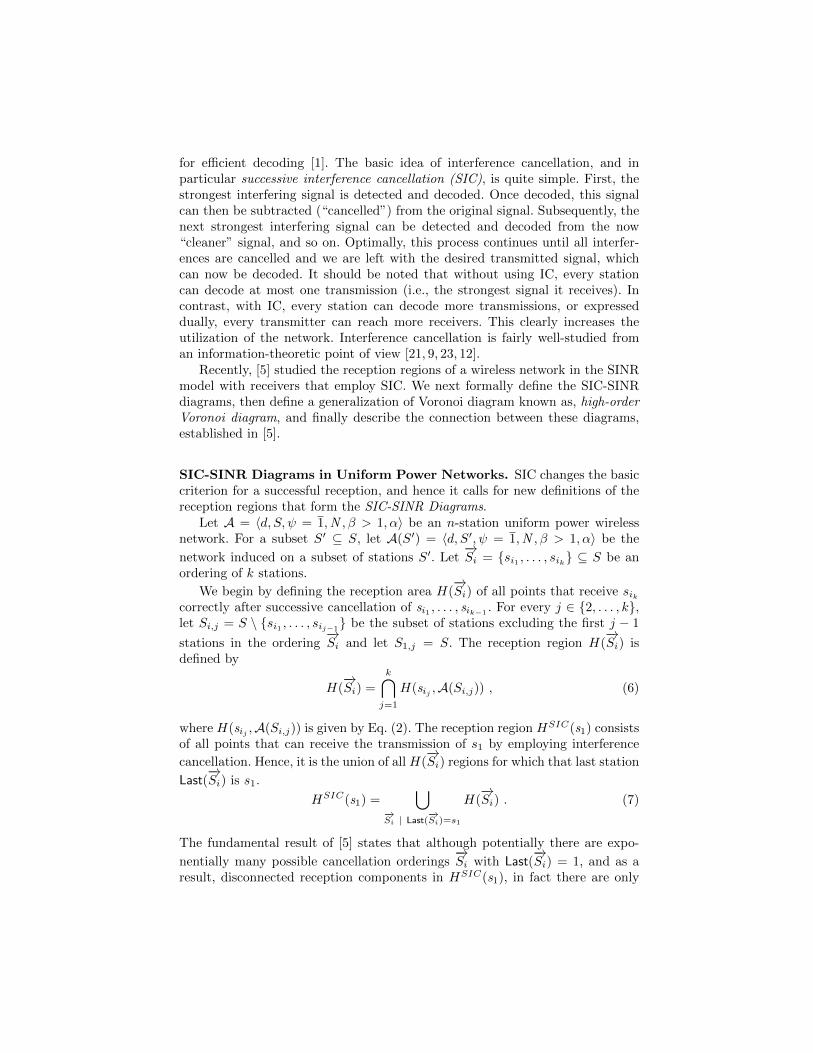
convex as well. Schematic illustration for k = 2 is provided in Fig. 4. For example,the region Vor(s1, s2) consists of all points whose nearest neighbor is s1 andwhose second nearest neighbor is s2. Similarly, the region Vor(s2, s1) consistsof all points whose nearest neighbor is s2 and whose second nearest neighbor iss1.

SIC-SINR diagrams and Ordered Order-k Voronoi diagrams. The re-

lation between a nonempty reception region H(−→Si),

−→Si = si1 , . . . , sik and an

nonempty ordered order-k polygon Vor(−→Si) is given in the next lemma.

Lemma 3 ([5]). H(−→Si) ⊆ Vor(

−→Si), for β ≥ 1 .

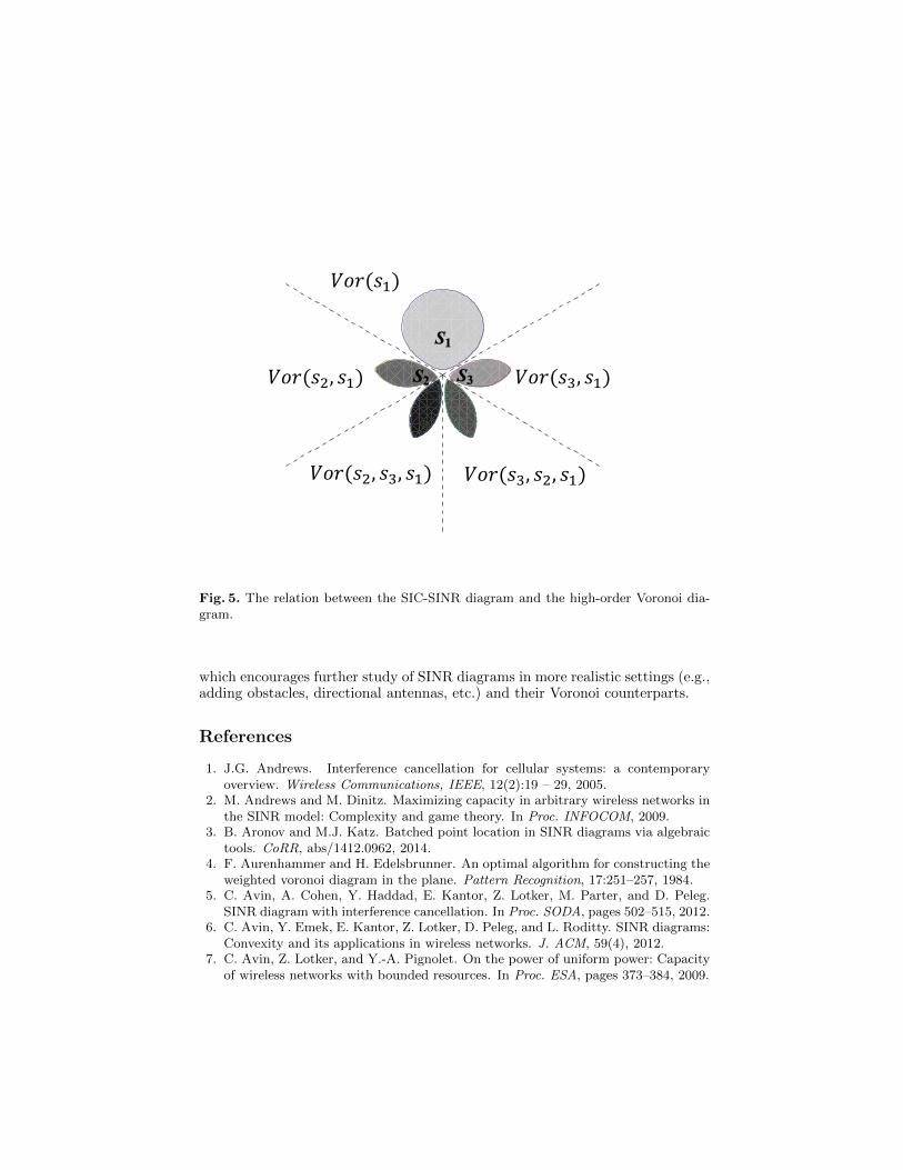
This relation was used by [5] to provide the following characterization of SIC-SINR reception regions: every region HSIC(si) is composed of a collection ofconvex regions, each of which is contained in corresponding cell of the higher-order Voronoi diagram. Fig. 5 illustrates this relation, and shows the receptionregion HSIC(s1). The light grey region H(s1) corresponds to the ordinary re-ception region with no cancellation. The black region H(s2, s3, s1) consists of

𝑉𝑜𝑟(𝑠1, 𝑠2)

𝑉𝑜𝑟(𝑠2, 𝑠1)

𝑉𝑜𝑟(𝑠2, 𝑠3) 𝑉𝑜𝑟(𝑠3, 𝑠2)

𝑉𝑜𝑟(𝑠3, 𝑠1)

𝑉𝑜𝑟(𝑠3, 𝑠1)

Fig. 4. A system of 3 points s1, s2, s3 and their ordered order-2 Voronoi diagram.

all points that first decoded s2, cancelled it, then decoded s3 and cancelled it,and finally were able to decode s1. Each of these connected reception regionsis fully contained in their corresponding high order Voronoi regions. For exam-ple, the black region H(s2, s3, s1) is contained in the high order Voronoi regionVor(s2, s3, s1) (i.e., the set of all points whose first nearest neighbor is s2, thens3 and finally s1.) Finally, SIC-SINR diagrams are also shown to be related tohyperplane arrangements [10], a plane-tessellation formed by the intersection ofthe set of

(n2

)hyperplane of pairs in S.

Applications. The connections to both high-order Voronoi diagram and hyper-plane arrangements play a key role in [5] where it used to provide to (1) thetopological characterization of SIC-SINR regions and (2) algorithms for thesediagrams. Specifically, these connections are used for establishing a bound ofO(n2d+1) on the number of components in d-dimensional n-station networks.In addition, they yeild algorithmic applications for drawing and maintainingSIC-SINR diagram as well as for answering efficiently point-location queries.

6 Final Note: Towards Wireless Computational Geometry

A major long-term goal of the study of SINR diagrams is to develop the areaof “wireless computational geometry” in which SINR diagrams play a role thatis similar to that of Voronoi diagrams in computational geometry. Indeed, thisreview aimed at highlighting the intimate connections between these models

𝑉𝑜𝑟(𝑠1)

𝑉𝑜𝑟(𝑠2, 𝑠1)

𝑉𝑜𝑟(𝑠2, 𝑠3, 𝑠1) 𝑉𝑜𝑟(𝑠3, 𝑠2, 𝑠1)

𝑉𝑜𝑟(𝑠3, 𝑠1)

Fig. 5. The relation between the SIC-SINR diagram and the high-order Voronoi dia-gram.

which encourages further study of SINR diagrams in more realistic settings (e.g.,adding obstacles, directional antennas, etc.) and their Voronoi counterparts.

References

1. J.G. Andrews. Interference cancellation for cellular systems: a contemporaryoverview. Wireless Communications, IEEE, 12(2):19 – 29, 2005.

2. M. Andrews and M. Dinitz. Maximizing capacity in arbitrary wireless networks inthe SINR model: Complexity and game theory. In Proc. INFOCOM, 2009.

3. B. Aronov and M.J. Katz. Batched point location in SINR diagrams via algebraictools. CoRR, abs/1412.0962, 2014.

4. F. Aurenhammer and H. Edelsbrunner. An optimal algorithm for constructing theweighted voronoi diagram in the plane. Pattern Recognition, 17:251–257, 1984.

5. C. Avin, A. Cohen, Y. Haddad, E. Kantor, Z. Lotker, M. Parter, and D. Peleg.SINR diagram with interference cancellation. In Proc. SODA, pages 502–515, 2012.

6. C. Avin, Y. Emek, E. Kantor, Z. Lotker, D. Peleg, and L. Roditty. SINR diagrams:Convexity and its applications in wireless networks. J. ACM, 59(4), 2012.

7. C. Avin, Z. Lotker, and Y.-A. Pignolet. On the power of uniform power: Capacityof wireless networks with bounded resources. In Proc. ESA, pages 373–384, 2009.

8. F. Baccelli and B. Blaszczyszyn. Stochastic geometry and wireless networks volume1: Theory. Foundations and Trends in Networking., 3:249–449, 2009.

9. M. Costa and A. El-Gamal. The capacity region of the discrete memoryless in-terference channel with strong interference. IEEE Trans. Inf. Th., 33:710–711,1987.

10. H. Edelsbrunner. Algorithms in Combinatorial Geometry. Springer-Verlag, 1987.11. H. Edelsbrunner, D. Kirkpatrick, and R. Seidel. On the shape of a set of points in

the plane. IEEE Trans. Inf. Th., 29(4):551–559, 1983.12. R.H. Etkin, D.N.C. Tse, and H. Wang. Gaussian interference channel capacity to

within one bit. IEEE Trans. Inf. Th., 54(12):5534–5562, 2008.13. A. Goldsmith. Wireless Communications. Cambridge University Press, 2005.14. O. Goussevskaia, R. Wattenhofer, M.M. Halldorsson, and E. Welzl. Capacity of

arbitrary wireless networks. In Proc. INFOCOM, pages 1872–1880, 2009.15. P. Gupta and P.R. Kumar. The capacity of wireless networks. IEEE Trans. Inf.

Th., 46(2):388–404, 2000.16. M.M. Halldorsson and R. Wattenhofer. Wireless communication is in APX. In

Proc. ICALP, pages 525–536, 2009.17. E. Kantor, Z. Lotker, M. Parter, and D. Peleg. The topology of wireless commu-

nication. In Proc. STOC, 2011.18. T. Moscibroda. The worst-case capacity of wireless sensor networks. In Proc.

IPSN, pages 1–10, 2007.19. A. Okabe, B. Boots, K. Sugihara, and S.N. Chiu. Spatial Tesselations. Princeton

University Press, 1992.20. A. Ozgur, O. Leveque, and D. Tse. Hierarchical cooperation achieves optimal

capacity scaling in ad hoc networks. IEEE Trans. Inf. Th., 53:3549–3572, 2007.21. H. Sato. The capacity of the gaussian interference channel under strong interfer-

ence. IEEE Trans. Inf. Th., 27(6):786–788, 1981.22. D. Tse and P. Viswanath. Fundamentals of Wireless Communication. Cambridge

University Press, 2005.23. A.J. Viterbi. Very low rate convolution codes for maximum theoretical perfor-

mance of spread-spectrum multiple-access channels. IEEE J. Selected Areas inCommunications, 8(4):641–649, 1990.