1

ON THE RATIO-CORRELATION REGRESSION METHOD1

David A. Swanson Department of Sociology and

Center for Sustainable Suburban Development University of California Riverside

(David.swanson@ ucr.edu)

Jeff Tayman Department of Economics

University of San Diego San Diego (jtayman@san.rr.com)

2

Introduction

Regression-based methods for estimating population date back to E. C. Snow (1911), who

published, “The application of the method of multiple correlation to the estimation of post-censal

populations” in the Journal of the Royal Statistical Society. Snow’s paper represents the first

published description of the use of multiple regression in the estimation of population. It also

discusses other methods, pointing out their strengths and weaknesses, then describes the model

framework and the data used in the regression application, and applies it to districts in the U. K. In

addition to being the first published report in English of the use of regression for population

estimates, it sets the stage for subsequent papers by discussing it relative to other methods. A

discussion is published with the paper that contains many important insights that are today

commonplace in the use of multiple regression not only for making population estimates, but for

general use.

One of the insights (Snow, 1911: 625) is given by David Heron, who suggests that one of the

shortcomings acknowledged by Snow was to “control” the sum of the estimates for individual

districts to an estimate for the who country (“Estimate for the whole country/sum of estimates for

individual districts). Another is provided by G. Udny Yule, who contributed substantially to the

development of multiple regression as a modern analytic technique (Stigler, 1986: 345-361). Yule

(Snow, 1911: 621) noted that Snow demonstrated that a multiple regression model built using data

over one decade had coefficients that could be used for the subsequent decade with the insertion of

the new set of values for the independent variables. Yule also agreed with Snow that the ex post

facto tests performed by Snow suggested that using variables constructed on relative (percent)

change would perform better than variables constructed on the basis of absolute change (Snow,

1911: 622). Finally, among many comments that are useful still today for those interested in

regression based methods for estimating population, are the following: Greenwood’ remarks on the

3

impact of skewed distributions (Snow, 1911: 626); Baines’ (Snow, 1911: 626) comments on using

ratios, and the importance of data quality by virtually all of the discussants (Snow, 1911: 621-629).

Snow’s (1991) seminal paper is based on the premise that the relationship between symptomatic

indicators and the corresponding population remains unchanged over time. His work and the

insights provided by the discussants of his paper have led to three related but distinct approaches:

ratio correlation; difference correlation; and average ratio methods.

Ratio Correlation and Its Variants

The most common regression-based approach data to estimating the total population of a given

area is the ratio-correlation method. Introduced and tested by Schmitt and Crosetti (1954) and again

tested by Crosetti and Schmitt (1956), this multiple regression method involves relating between

changes in several variables known as symptomatic indicators on the one had to population changes

on the other hand. The symptomatic indicators that are used reflect the variables related to

population change that are available and of them, those that yield an optimal model. Examples of

symptomatic variable that have been used for this purpose are births, deaths, school enrollment, tax

returns, motor vehicle registrations, employment data, and registered voters. The ratio-correlation

method is used where a set of areas (e.g., counties) are structured into a geographical hierarchy (e.g.

the populations of counties within a given state sum to the total state population). It proceeds in two

steps. The first is the construction of the model and the second is its implementation – actually

using it to create estimates for given years.

Because the method looks at change, population data from two successive censuses are needed

to construct the model along with data for the same years representing the symptomatic indicators.

During its implementation step the ratio-correlation method requires symptomatic data representing

4

the year for which an estimate is desired and an estimate of the population for the highest level of

geography (e.g., the state as a whole) that is independent of the ratio-correlation model.

The ratio-correlation method expresses the relationship between (1) the change over the

previous intercensal period (e.g., 1990 to 2000) in an area’s share (e.g., a given county) of the total

for the parent area (e.g., the state as a whole) for several symptomatic series and (2) the change in

an area’s share of the population of the parent area. The method can be employed to make

estimates for either the primary or secondary political, administrative and statistical divisions of a

country (Bryan, 2004). In the U.S., the variables selected usually vary from state to state and

because of due the small number of counties in some states, certain states were combined and

estimated in one regression equation.

In general terms, the ratio correlation model is formally described as follows (Swanson and

Beck, 1994):

Pi,t = a0 + ∑(bj)*Si,j,t + εi [1a]

where

a0 = the intercept term to be estimated

bj = the regression coefficient to be estimated

εi = the error term j = symptomatic indicator (1 ≤ j ≤ k)

i = subarea (1 ≤ j ≤ n)

t = year of the most recent census

and

Pi,t = (Pi,t/∑ Pi,t) /(Pi,t-z/∑ Pi,t-z) [1b]

Si,j,t = (Si,t/∑ Si,t)j /(Si,t-z/∑ Si,t-z) j [1c]

where

z = number of years between each census for which data are used to construct the model

5

p = population

s = symptomatic indicator

Once a ratio correlation model is constructed, a set of population estimates for time t+k is

developed in a series of six steps. First, (Si,t+k/∑ Si,t+k)j is substituted into the numerator of the right

side of Equation [1c] for each symptomatic indicator j and (Si,t/∑ Si,t) j into the denominator of the

right side of Equation [1c] for each symptomatic indicator j, which yields Si,j,t+k. Second, the

updated model with the preceding substitution of symptomatic data for time t+k is used to estimate

Pi,t+k. Third, (Pi,t/∑ Pi,t) is substituted into the denominator of Pi,t+k, which yields Pi,t+k = (Pi,t+k/∑

Pi,t+k)/(Pi,t/∑ Pi,t), where ∑ Pi,t+k) represents the independently estimated population of the “parent”

area of the i subareas for time t+k (Note that this estimate is given in boldface and is done by a

method exogenous to the ratio-correlation model (e.g., a component method)). Fifth, since Pi,t+k ,

(Pi,t/∑ Pi,t) and ∑ Pi,t+k are all known values, the equation Pi,t+k = (Pi,t+k/∑ Pi,t+k) /(Pi,t/∑ Pi,t) is

manipulated to yield an estimate of the population of area i at time t+k:

^ (Pi,t+k) *(Pi,t/∑ Pi,t) *(∑ Pi,t+k) = Pi,t+k [1d]

As Equation [1d] shows, it is important to remember that an independent estimate of the

population for the “parent” geography (∑Pi,t+k) of the i subarea is required when using the ratio-

correlation model to generate population estimates. The sixth and final step is to effect a final

“control” so that the sum of the i subarea population estimates is equal to the independently

estimated population for the parent of these i subareas: ∑ Pi,t+k = ∑Pi,t+k, which is accomplished as

follows:

Pi,t+k = (Pi,t+k /∑ Pi,t+k )*( ∑Pi,t+k). [1e]

6

As an empirical example of ratio-correlation model, we use data for the 39 counties of

Washington State. We used excel to construct a ratio-correlation model using 1990 and 2000 census

data in conjunction with three symptomatic indicators: (1) registered voters; (2) registered

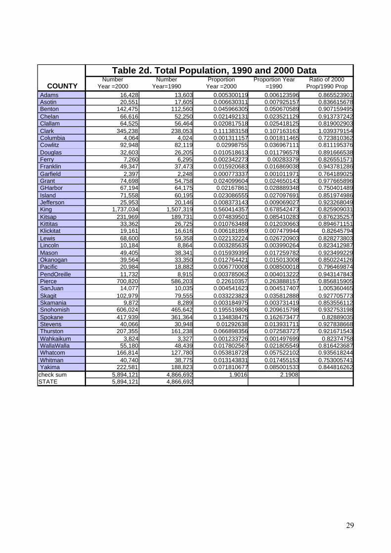
automobiles, and (3) public school enrollment in grades 1-8. The raw 1990 and 2000 input data for

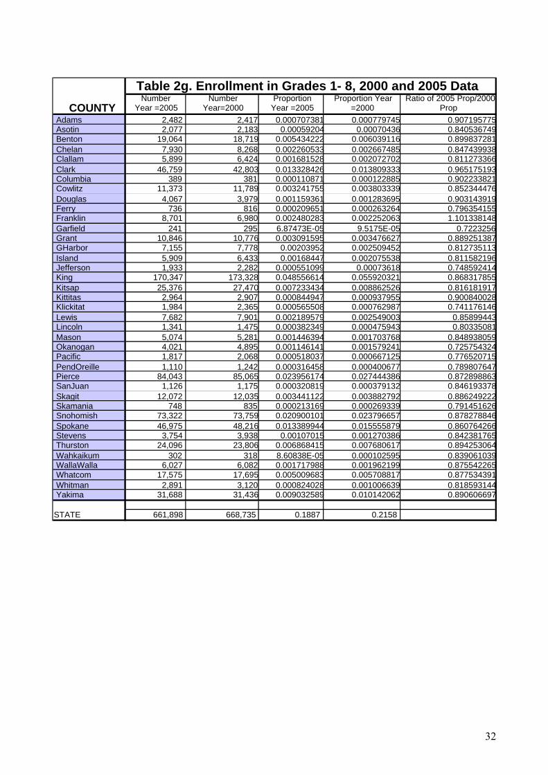
this model are provided in an appendix as tables 2.a through 2.d. We then use 2005 symptomatic

indicators to construct a set of county estimates for 2005. The input data for 2000 and 2005, along

with the results of the calculations leading to the estimates are shown as tables 2.e through 2.h in the

appendix.

A summary of the model and its characteristics is provided in Exhibit 1.

Exhibit 1. Example Ratio Correlation Model

Although the coefficient for Voters is not statistically significant, we elected to retain this

symptomatic indicator in the model so that we would have a model with three independent

variables, a feature that as explained later, can assist in dealing with “model invariance.”

Pi,t = 0.195 + (0.0933*Voters) + (0.3362*Autos) + (0.3980*Enroll) [p<.001] [p= 0.14] [p < .001] [p<.001] where Pi,t = (Pi,2000/∑ Pi,2000) /(Pi,1990/∑ Pi,1990)

Si,1,t = (Votersi,2000/∑ Votersi,2000) /(Votersi,1990/∑ Votersi,1990)

Si,2,t = (Autosi,2000/∑ Autosi,2000) /(Autosi,1990/∑ Autosi,1990)

Si,3,t = (Enrolli,2000/∑ Enrolli,2000) /(Enrolli,1990/∑ Enrolli,1990)

R2 = 0.794

adj R2 = 0.776

7

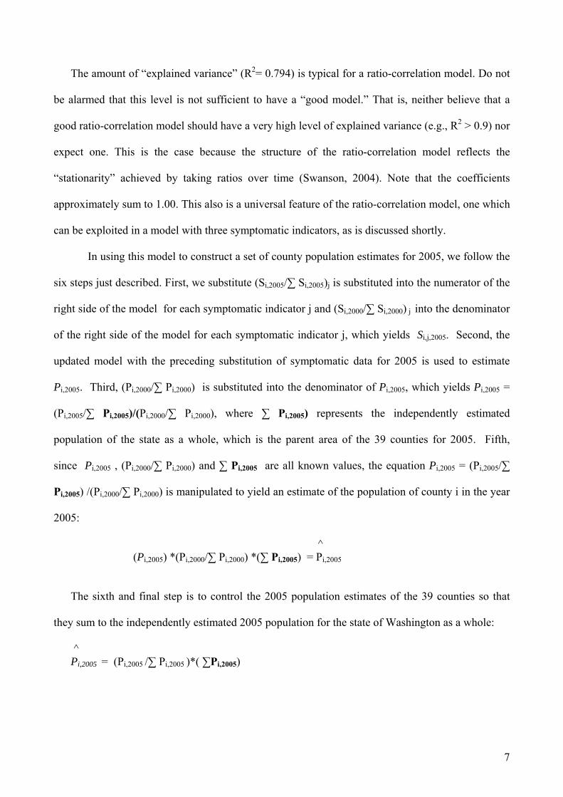
The amount of “explained variance” (R2= 0.794) is typical for a ratio-correlation model. Do not

be alarmed that this level is not sufficient to have a “good model.” That is, neither believe that a

good ratio-correlation model should have a very high level of explained variance (e.g., R2 > 0.9) nor

expect one. This is the case because the structure of the ratio-correlation model reflects the

“stationarity” achieved by taking ratios over time (Swanson, 2004). Note that the coefficients

approximately sum to 1.00. This also is a universal feature of the ratio-correlation model, one which

can be exploited in a model with three symptomatic indicators, as is discussed shortly.

In using this model to construct a set of county population estimates for 2005, we follow the

six steps just described. First, we substitute (Si,2005/∑ Si,2005)j is substituted into the numerator of the

right side of the model for each symptomatic indicator j and (Si,2000/∑ Si,2000) j into the denominator

of the right side of the model for each symptomatic indicator j, which yields Si,j,2005. Second, the

updated model with the preceding substitution of symptomatic data for 2005 is used to estimate

Pi,2005. Third, (Pi,2000/∑ Pi,2000) is substituted into the denominator of Pi,2005, which yields Pi,2005 =

(Pi,2005/∑ Pi,2005)/(Pi,2000/∑ Pi,2000), where ∑ Pi,2005) represents the independently estimated

population of the state as a whole, which is the parent area of the 39 counties for 2005. Fifth,

since Pi,2005 , (Pi,2000/∑ Pi,2000) and ∑ Pi,2005 are all known values, the equation Pi,2005 = (Pi,2005/∑

Pi,2005) /(Pi,2000/∑ Pi,2000) is manipulated to yield an estimate of the population of county i in the year

2005:

^ (Pi,2005) *(Pi,2000/∑ Pi,2000) *(∑ Pi,2005) = Pi,2005

The sixth and final step is to control the 2005 population estimates of the 39 counties so that

they sum to the independently estimated 2005 population for the state of Washington as a whole:

^ Pi,2005 = (Pi,2005 /∑ Pi,2005 )*( ∑Pi,2005)

8

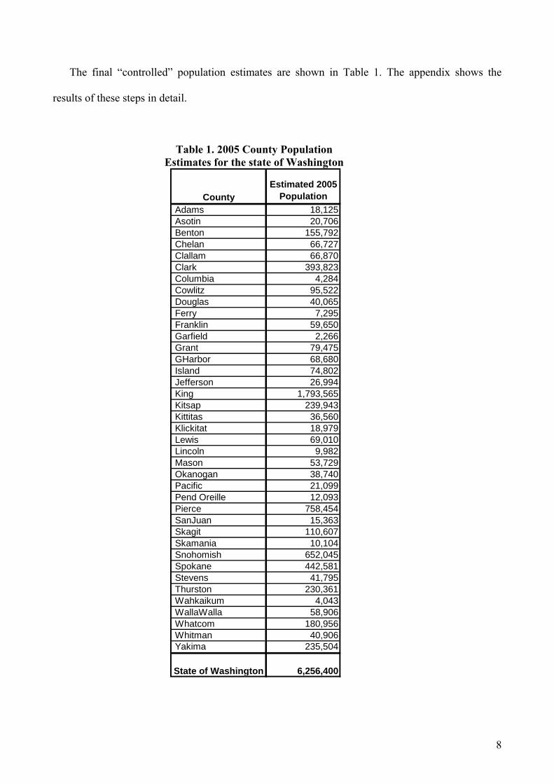
The final “controlled” population estimates are shown in Table 1. The appendix shows the

results of these steps in detail.

Table 1. 2005 County Population Estimates for the state of Washington

CountyEstimated 2005

Population Adams 18,125 Asotin 20,706 Benton 155,792 Chelan 66,727 Clallam 66,870 Clark 393,823 Columbia 4,284 Cowlitz 95,522 Douglas 40,065 Ferry 7,295 Franklin 59,650 Garfield 2,266 Grant 79,475 GHarbor 68,680 Island 74,802 Jefferson 26,994 King 1,793,565 Kitsap 239,943 Kittitas 36,560 Klickitat 18,979 Lewis 69,010 Lincoln 9,982 Mason 53,729 Okanogan 38,740 Pacific 21,099 Pend Oreille 12,093 Pierce 758,454 SanJuan 15,363 Skagit 110,607 Skamania 10,104 Snohomish 652,045 Spokane 442,581 Stevens 41,795 Thurston 230,361 Wahkaikum 4,043 WallaWalla 58,906 Whatcom 180,956 Whitman 40,906 Yakima 235,504

State of Washington 6,256,400

9

An acute observer may notice that except when k=z, the use of the model for estimating

population corresponds to a shorter length of time than that used to calibrate the model. For

example, if one constructs a model using 1990 and 2000 data for the 39 counties in the state of

Washington it corresponds to a ten year period of change in both population shares and shares of

symptomatic variables. However, in using this same model to estimate the populations of the 39

counties in 2003, the time period now corresponds to a three year period of change in both

population shares and shares of symptomatic variables. Swanson and Tedrow (1989) addressed this

temporal inconsistency by using a logarithmic transformation. They called the resulting model the

“rate-correlation” model. This is one of several variants of the basic ratio-correlation regression

technique. Another is known as the “difference correlation” method. Similar in principle to the

ratio-correlation method, the difference correlation method differs in its construction of a variable

that is used to reflect change over time. Rather than making ratios out of the two proportions at two

points in time, the difference correlation method employs the differences between proportions

(Schmitt and Grier, 1966; O’Hare 1976; Swanson, 1978a). Another variant was proposed by

Namboodiri and Lalu (1971). Known as the “average regression” technique, Namboodiri and Lalu

(1971) examined the use of the simple, unweighted average of the estimates provided by a number

of simple regression equations, each of which relates the population ratio to one symptomatic

indicator ratio (As discussed in Chapter 9, this turns out to be very similar to using an average of

several censal ratio estimates). Using the insights provide by Namboodiri and Lalu (1971), Swanson

and Prevost (1985) demonstrated that the ratio-correlation model can be interpreted as a

demographic form of “synthetic estimation” that is composed of a set of weighted censal-ratio

estimates, with the regression coefficients serving as the weights – a topic we cover toward this end

of this exposition.

Bryan (2004) observes that one of the shortcomings of the ratio-correlation method and related

techniques is that substantial time lags can occur in obtaining the symptomatic indicators needed for

10

producing a current population estimate. That is, suppose that it is the year 2014 and a current

(2014) estimate is desired, but the most current symptomatic indicators are for 2012. What can one

do? One answer to this question is “lagged ratio-correlation,” which was introduced by Swanson

and Beck (1994). In this variant of ratio-correlation, the ratios of proportional symptomatic

indicators precede the ratios of population proportions by “m” years in model construction so that:

Si,jt-m = (Si,t-m/∑ Si,t-m)j /(Si,(t-m)-z/∑ Si,(t-m)-z) j [1f]

where

m = number of years that symptomatic indicators precede the population proportions

When the lagged ratio-correlation is used to estimate a population, the only change to the six

steps described earlier for the basic form of ratio-correlation is that (Si,t+k/∑ Si,t+k)j is substituted

into the numerator of the right side of Equation [1c] for each symptomatic indicator j in place of

(Si,(t-m)+k/∑ Si,(t-m)+k)j and /(Si,(t-m)/∑ Si,(t-m)) j into the denominator of the right side of Equation [1c]

for each symptomatic indicator j in place of (Si,t/∑ Si,t) j.

Because ratio-correlation and its variants are grounded in regression, they are connected to the

inferential and other statistical tools that come with it (Swanson, 1989; Swanson and Beck, 1994).

In using these tools, it is important to point to keep in mind several important things. The first point

is that within this framework, "uncertainty" is generally based on the “frequentist” view of sample

error. Thus, as discussed by Swanson and Beck (1994), the construction of confidence intervals

around estimated values means, for example, that one perceives (whether implicitly or explicitly)

the following: the data used in model construction are a random sample drawn from a universe; the

model would fit perfectly were it not for random error; and, any subsequent observations of

independent variables placed into the model and used to generate dependent variables are drawn

from the same universe. Since a given model is constructed from data using observations from all

known cases (e.g., all 39 counties in Washington), the "universe" represented by the county data is a

11

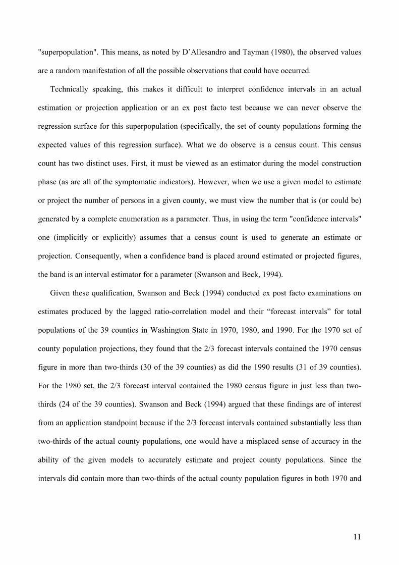
"superpopulation". This means, as noted by D’Allesandro and Tayman (1980), the observed values

are a random manifestation of all the possible observations that could have occurred.

Technically speaking, this makes it difficult to interpret confidence intervals in an actual

estimation or projection application or an ex post facto test because we can never observe the

regression surface for this superpopulation (specifically, the set of county populations forming the

expected values of this regression surface). What we do observe is a census count. This census

count has two distinct uses. First, it must be viewed as an estimator during the model construction

phase (as are all of the symptomatic indicators). However, when we use a given model to estimate

or project the number of persons in a given county, we must view the number that is (or could be)

generated by a complete enumeration as a parameter. Thus, in using the term "confidence intervals"

one (implicitly or explicitly) assumes that a census count is used to generate an estimate or

projection. Consequently, when a confidence band is placed around estimated or projected figures,

the band is an interval estimator for a parameter (Swanson and Beck, 1994).

Given these qualification, Swanson and Beck (1994) conducted ex post facto examinations on

estimates produced by the lagged ratio-correlation model and their “forecast intervals” for total

populations of the 39 counties in Washington State in 1970, 1980, and 1990. For the 1970 set of

county population projections, they found that the 2/3 forecast intervals contained the 1970 census

figure in more than two-thirds (30 of the 39 counties) as did the 1990 results (31 of 39 counties).

For the 1980 set, the 2/3 forecast interval contained the 1980 census figure in just less than two-

thirds (24 of the 39 counties). Swanson and Beck (1994) argued that these findings are of interest

from an application standpoint because if the 2/3 forecast intervals contained substantially less than

two-thirds of the actual county populations, one would have a misplaced sense of accuracy in the

ability of the given models to accurately estimate and project county populations. Since the

intervals did contain more than two-thirds of the actual county population figures in both 1970 and

12

1990 and nearly two-thirds in 1980, they argued that the results of this case study revealed an

intuitively appealing view of the accuracy of these particular models (Swanson and Beck, 1994).

The findings by Swanson and Beck (1994) suggest that, among other useful features, one can

construct confidence and “forecast” intervals around the estimates produced by ratio-correlation

and its variants that are both statistically and substantively meaningful.

Given that the input data are of good quality, the accuracy of the regression-based techniques

largely depends upon the validity of the central underlying assumption: that the observed statistical

relationship between the independent and dependent variables in the past intercensal period will

persist in the current postcensal period. The adequacy of this assumption (that the model is

invariant) is dependent on several conditions (Swanson, 1980; Mandell and Tayman, 1982;

McKibben and Swanson, 1997; Tayman and Schafer, 1985).

In an attempt to deal with model invariance, Ericksen (1973, 1974) introduced a method of

post-censal estimation in which the symptomatic information is combined with sample data by

means of a regression format. He considered combining symptomatic information on births, deaths,

and school enrollment with sample data from the Current Population Survey. Swanson (1980) took

a different approach to the issue of model invariance and presented a mildly restricted procedure for

using a theoretical causal ordering and principles from path analysis to provide a basis for

modifying regression coefficients in order to improve the estimation accuracy of the ratio-

correlation method of population estimation.

Ridge Regression also represents a method for dealing with model invariance. Swanson

(1978b) and D’Allesandro and Tayman (1980) examined this approach to multiple regression and

found that it offered some benefits. Ridge Regression also represents a way to deal with another

possible problem with the regression approach, which is multi-collinearity, a condition whereby the

independent variables are all highly correlated. This condition can result in type II errors (finding

that given coefficients are not shown to be statistically significant when in fact they are) when one

13

evaluates the statistical significance of the coefficients associated with the symptomatic indicators

used in a given model. One also can use the stand diagnostic tools associated with regression to

evaluate and this issue and overcome it without resorting to ridge regression, if an evaluation

suggests it is present (Fox, 1991). Swanson (1989) demonstrated another way to deal with model

invariance by using the statistical properties of the ratio-correlation method in conjunction with the

Wilcoxon matched-pairs signed rank test and the “rank-order” procedure he introduced (Swanson

1980).

Judgment is also important in the application of ratio-correlation, as the analyst must take into

account the reliability and consistency of coverage of each variable (Tayman and Schafer, 1985).

The increasing availability of administrative data allows many possible combinations of variables.

High correlation coefficients for two past intercensal periods would suggest that the degree of

association of the variables is not changing very rapidly. In such a case, the regression based on the

last intercensal period should be applicable to the current postcensal period. Furthermore, it is

assumed that deficiencies in coverage in the basic data series will remain constant, or change very

little, in the present period (Tayman and Schafer, 1985).

In addition to the issue of time lags in the availability of symptomatic indicators, Bryan (2004),

notes two other shortcomings of regression-based techniques: (1) the use of multiple and differing

variables (oftentimes depending on the place being estimated) and in some instances averaging the

results of multiple estimates makes it very difficult to decompose error; and (2) this process may

compromise the comparability of estimates between different subnational areas. In regard to

decomposing error, this is a feature of all of the estimation methods that do not deal directly with

the components of population change. In regard to comparability, we note that this is an issue when

different regression models are used (e.g., the ratio-correlation model used to estimate the

populations of the 75 counties of Arkansas is different from the ratio-correlation model used to

estimate the populations of the 39 counties of Washington state.

14

In regard to the issue of decomposing error, McKibben and Swanson (1997) argue that at

least some of the shortcomings in accuracy of population estimates would be better understood by

linking these methods with the substantive socio-economic and demographic dynamics that clearly

must be underlying the changes in population that the methods are designed to measure. They

provide a case study of Indiana over two periods, 1970-1980 and 1980-1990, which was selected

because a common population estimation method exhibits a common problem over the two periods:

its coefficients change. The authors link these changes to Indiana's transition to a post-industrial

economy and describe how this transition operated through demographic dynamics that ultimately

affected the estimation model.

Ratio-Correlation and Synthetic Estimation

Before describing synthetic estimation and its relationship to the ratio-correlation method, it

is important to realize that synthetic estimation emerged from the field of survey research, as

statisticians grappled with the problem of trying to apply survey results for a large area (e.g., the

U.S. as a whole) to subareas (e.g., states) while maintaining validity and avoiding excessive costs.

Thus, as Swanson and Pol (2008) observe, there are two distinct traditions in regard to “small area

estimates,” (1) demographic; and (2) statistical:

“Demographic methods are used to develop estimates of a total population as well as the ascribed characteristics – age, race, and sex - of a given population. Statistical methods are largely used to estimate the achieved characteristics of a population – educational attainment, employment status, income, and martial status, for example Among survey statisticians, the demographer’s definition of an estimate is generally termed an "indirect estimate" because unlike a sample survey, the data used to construct a demographic estimate are symptomatic indicators of population change (e.g., K-12 enrollment data, births, deaths,) and do not directly represent the phenomenon of interest. Among demographers, the term "indirect estimate" has a different meaning.”

So, in the field of demography a direct estimate refers to the measurement of demographic

phenomena using data that directly represent the phenomena of interest, while among statisticians,

it is used to describe estimates obtained by survey sampling. In terms of an indirect estimate,

15

demographers, usually use this term in referring to the measurement of demographic phenomena

using data that do not directly represent the phenomena of interest (e.g., a child woman ratio instead

of a crude birth rate). Among survey statisticians, this term refers to an estimate not based on a

sample survey, for example, a model based estimate (Schaible, 1993).

As a bit of history on the emergence of synthetic estimation, Ford (1981) notes that the

problem of constructing county or other small area estimates from survey data has been an

important topic and large-scale surveys and even complete census counts were often used to solve

the problem. Because of the resource needs of this approach, attention turned to possible

alternatives for obtaining small area information in the 1970s. (U.S. NCHS, 1968; Ford, 1981). One

of the alternatives that gained a lot of attention was synthetic estimation, which according to Ford

(1981) emerged because of a 1978 workshop on Synthetic Estimates for Small Area Estimates co-

sponsored by the National Institute on Drug Abuse (NIDA) and the National Center for Health

Statistics (NCHS). This same workshop resulted in a monograph edited by Steinberg (1979).

In the “Introduction” to the NIDA/NCHS monograph, Steinberg (1979) cites “The Radio

Listening Survey,” discussed in Hansen, Hurwitz and Madow (1953) as an early example of the

employment of the synthetic method. In this survey, questionnaires were mailed to about 1,000

families in each of 500 county areas and personal interviews were conducted with a sub-sample of

the families in 85 of these count areas who were mailed questionnaires (Hansen, Hurwitz, and

Madow (1953: 483-484). Knowing in advance that the mail-out portion would yield a low level of

responses (about 20 percent of those mailed questionnaires responded), the data collected in the

personal interviews were used to obtain estimates not affected by non-response. The relationships

between the data in the 85 county areas that were collected from the personal interviews and the

mailed questionnaires were then applied to the county areas for which only mail-out/mail-back was

done to improve the estimates for these areas (Hansen, Hurwitz, and Madow (1953: 483). While the

16

radio listening study did no use the hallmark of synthetic estimation, which is taking information

from a “parent” area and applying it to its subareas, the idea behind it is similar.

In most cases, synthetic estimation is used to estimate “achieved characteristics” and often

rely on estimates made by demographers of total populations and their achieved characteristics

(e.g., age, race, and sex) in developing the estimates (Causey, 1988; Cohen and Zhang, 1988;

Gonzalez and Hoza, 1978; Levy, 1979). However, it need not be confined to this use. Before we

turn to a demographic interpretation of synthetic estimation, it is useful to spend some time on its

statistical interpretation.

Cohen and Zhang (1988) provide an informal statistical definition of a synthetic estimator

that we adapt as follows. First, assume that one is interested in obtaining estimates of an unknown

characteristic, xi over a set of i sub-regions (i = 1,…,n) . Second, suppose one has census counts pi,

(i =l ,…,n), for each of the sub-regions and both a census count, P, and a “known” value of X, for

the parent region, where ∑pi. = P and ∑xi. = X, respectively. Third, suppose that the estimated

values of xi for the subareas must sum to the known value X for the parent area. In this case, Cohen

and Zhang (1988: 2) define the statistical synthetic estimate as:

^

x i = (X/P)* (pi) . [2]

Basically, Equation [2] shows that the estimated characteristic (xi) for a given subarea i is

found by multiplying the known value of population for sub-area i, pi, by the “known” ratio of the

characteristic (X) to population (P) for the parent area. It is inevitably the case that the “known”

value of X for the parent area is taken from a sample survey (U.S. NCHS, 1968). Cohen and Zhang

(1988) go on to show how the basic idea given in Equation [2] can be extended to include

demographic subgroups (e.g., by age, race, and sex). Similar examples are provided by Levy

(1979).

17

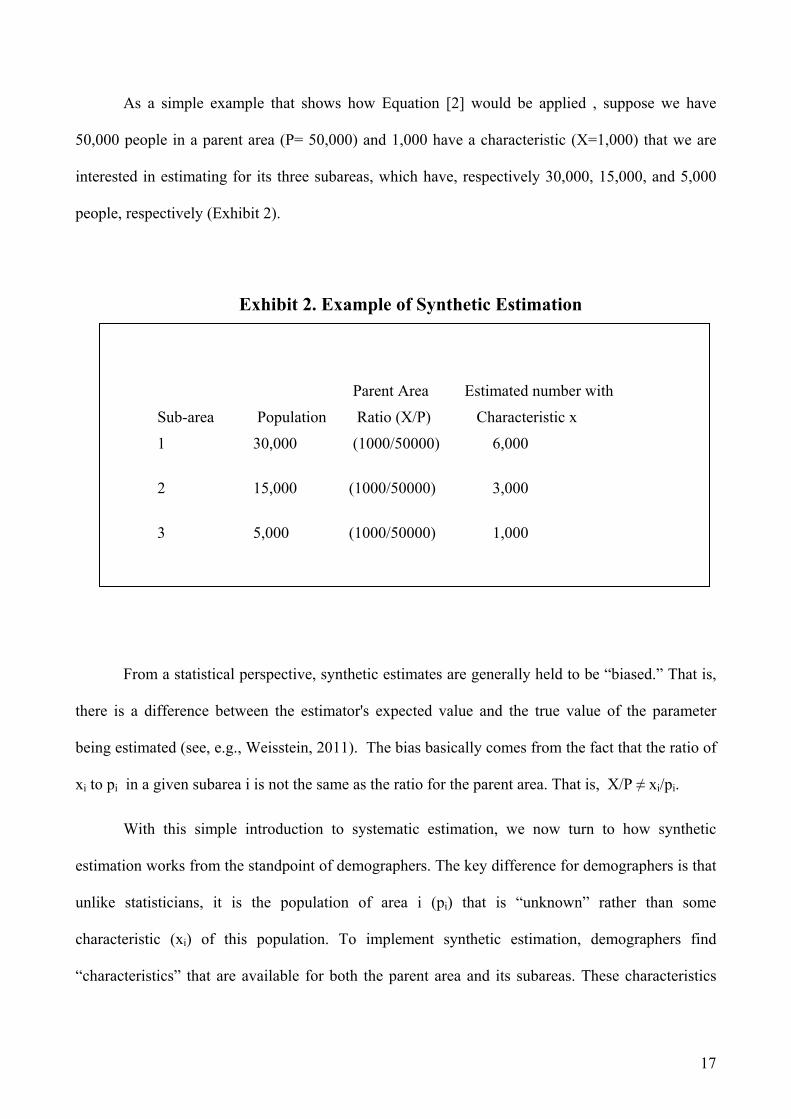
As a simple example that shows how Equation [2] would be applied , suppose we have

50,000 people in a parent area (P= 50,000) and 1,000 have a characteristic (X=1,000) that we are

interested in estimating for its three subareas, which have, respectively 30,000, 15,000, and 5,000

people, respectively (Exhibit 2).

Exhibit 2. Example of Synthetic Estimation

From a statistical perspective, synthetic estimates are generally held to be “biased.” That is,

there is a difference between the estimator's expected value and the true value of the parameter

being estimated (see, e.g., Weisstein, 2011). The bias basically comes from the fact that the ratio of

xi to pi in a given subarea i is not the same as the ratio for the parent area. That is, X/P ≠ xi/pi.

With this simple introduction to systematic estimation, we now turn to how synthetic

estimation works from the standpoint of demographers. The key difference for demographers is that

unlike statisticians, it is the population of area i (pi) that is “unknown” rather than some

characteristic (xi) of this population. To implement synthetic estimation, demographers find

“characteristics” that are available for both the parent area and its subareas. These characteristics

Parent Area Estimated number with

Sub-area Population Ratio (X/P) Characteristic x

1 30,000 (1000/50000) 6,000

2 15,000 (1000/50000) 3,000

3 5,000 (1000/50000) 1,000

18

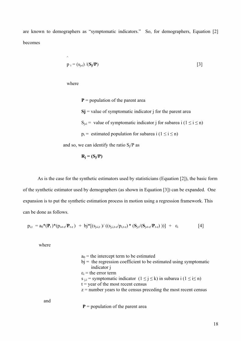
are known to demographers as “symptomatic indicators.” So, for demographers, Equation [2]

becomes

^

p i = (sj,i) /(Sj/P) [3]

where

P = population of the parent area

Sj = value of symptomatic indicator j for the parent area

Sj,i = value of symptomatic indicator j for subarea i (1 ≤ i ≤ n)

pi = estimated population for subarea i (1 ≤ i ≤ n)

and so, we can identify the ratio Sj/P as

Rj = (Sj/P)

As is the case for the synthetic estimators used by statisticians (Equation [2]), the basic form

of the synthetic estimator used by demographers (as shown in Equation [3]) can be expanded. One

expansion is to put the synthetic estimation process in motion using a regression framework. This

can be done as follows.

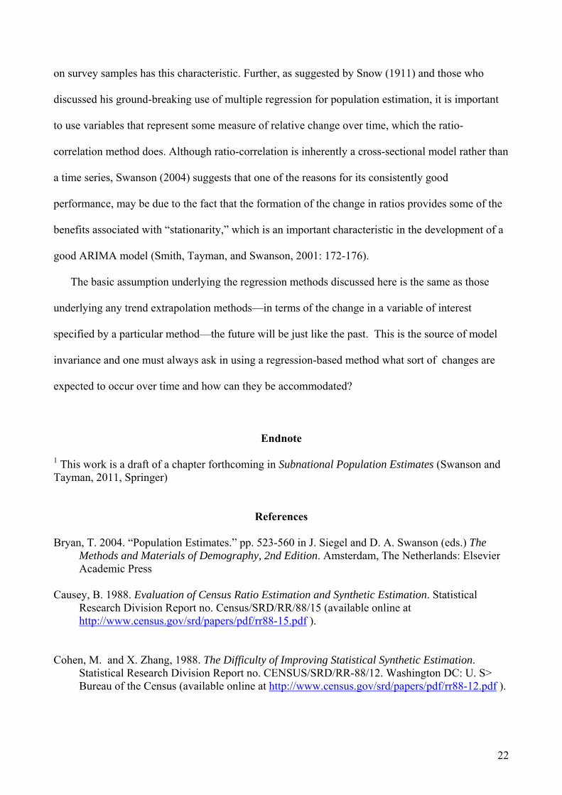
pi,t = a0*(Pt )*(pi,t-z/Pt-z ) + bj*[(sj,i,t )/ ((sj,i,t-z/pi,t-z) * (Sj,t/(Sj,t-z/Pt-z) ))] + εi [4]

where

a0 = the intercept term to be estimated bj = the regression coefficient to be estimated using symptomatic indicator j

εi = the error term s j,i = symptomatic indicator (1 ≤ j ≤ k) in subarea i (1 ≤ i≤ n) t = year of the most recent census z = number years to the census preceding the most recent census

and P = population of the parent area

19

Sj = value of symptomatic indicator j for the parent area

pi = estimated population for subarea i (1 ≤ i ≤ n)

Once the preceding regression model is constructed, it can be used to estimate the population of

each area i for a year k years subsequent to the last census (time =t) as follows:

^

pi,t+k = [a0*(Pt+k )*(pi,t/Pt )] + [bj*((sj,i,t+k )/ ((sj,i,t/pi,t) * (Sj,t+k/(Sj,t/Pt) )))] [5]

Equations [4] and [5] should be familiar. They can be algebraically manipulated to become a

bivariate form (i.e., a regression model with only one independent variable) of the ratio-correlation

model discussed earlier, which we show here. First, borrowing from Equation [1a], we show here

the simple bivariate ratio-correlation regression model that is algebraically equivalent to Equation

[5]

Pi,t = a0 + (bj)*Si,jt + εi [6]

where

a0 = the intercept term to be estimated

bj = the regression coefficient to be estimated

εi = the error term j = symptomatic indicator (1 ≤ j ≤ k)

i = subarea (1 ≤ j ≤ n)

t = year of the most recent census

and

Pi,t = (Pi,t/∑ Pi,t) /(Pi,t-z/∑ Pi,t-z) [7]

20

Si,jt = (Si,t/∑ Si,t)j /(Si,t-z/∑ Si,t-z) j [8]

where

z = number of years between each census for which data are used to construct the model p = population

s = symptomatic indicator

As was shown earlier, a set of population estimates can be done in a series of six

steps, which lead to the estimation version of Equation [6], which is algebraically equivalent to

Equation [5]:

^ (Pi,t+k) *(Pi,t/∑ Pi,t) *(∑ Pi,t+k) = Pi,t+k [9]

As discussed by Swanson and Prevost (1985), these equations show that the ratio-correlation

model can be viewed as a regression method that uses synthetic estimation (taking a ratio of change

for a given “rate” in a parent area and a “censal-ratio” to estimate a current population for area i).

Note that the intercept term, a0, shown in Equation [5] serves as a “weight” applied to an estimate of

pi at time t+k (pi,t+k) based on the proportion of the population in area i at the time of the last census,

t (pi,t) that is multiplied by the total of the parent area at time t+k (Pt+k). The regression coefficient,

bj, shown in Equation [5] also serves as a weight. In this case it is applied to the “synthetic

estimate” based on symptomatic indicator sj. As Swanson (1980) and Swanson and Prevost (1985)

observe, the regression coefficient in a ratio-correlation model sum to 1.00 (or very nearly so) in

virtually every model constructed, which means that as shown in Equation [5] the estimate of pi can

be viewed as a weighted average of synthetic estimates based on j symptomatic indicators.

In terms of strengths of the sample based methods that are aimed at generating what the

statisticians refer to direct estimates, they offer a well-understood approach that is less costly than

21

full enumerations along with estimates of their precision. In terms of their weaknesses, the cost of

sample surveys often precludes using them to develop usable information for small areas unless

they are supplemented by other methods such as synthetic estimation (Ghosh and Rao, 1994; Platek

et al., 1987; Rao, 2003). Jaffe (1951: 211) notes that while sample surveys are cheaper than full

enumerations, “demographic procedures” are cheaper than sample surveys; however, he also notes

that the “direct estimates” resulting from sample surveys can only be used for current estimates

since it is impossible to interview a past or future population. He goes to observe that only

“demographic procedures” can provide past, current, and future estimates. We note, however, that

these same ‘demographic procedures’ can be improved by using the statistical tools and

perspectives that have emerged from sampling, as this discussion of synthetic estimation illustrates.

Summary

Regression-based methods have very limited application in the preparation of estimates of

population composition, such as age-sex groups for small geographic areas. It is possible, of

course, to apply the age distribution at the last census date to a pre-assigned current total for the

area, or to extrapolate the last two census age distributions to the current date and apply the

extrapolated distribution to the current total. Spar and Martin (1979) found, for example, that the

ratio-correlation method is more accurate than others in estimating the populations of Virginia

counties by race and age.

While the ratio-correlation approach has its limitations, as suggested by this overview, it is clear

it has strong advantages, given the availability of good quality data to implement and test it. Among

its many advantages is the fact that regression has a firm foundation in statistical inference, which

leads to the construction of meaningful measures of uncertainty around the estimates it produces, as

demonstrated by Swanson and Beck (1994). No other population technique other than those based

22

on survey samples has this characteristic. Further, as suggested by Snow (1911) and those who

discussed his ground-breaking use of multiple regression for population estimation, it is important

to use variables that represent some measure of relative change over time, which the ratio-

correlation method does. Although ratio-correlation is inherently a cross-sectional model rather than

a time series, Swanson (2004) suggests that one of the reasons for its consistently good

performance, may be due to the fact that the formation of the change in ratios provides some of the

benefits associated with “stationarity,” which is an important characteristic in the development of a

good ARIMA model (Smith, Tayman, and Swanson, 2001: 172-176).

The basic assumption underlying the regression methods discussed here is the same as those

underlying any trend extrapolation methods—in terms of the change in a variable of interest

specified by a particular method—the future will be just like the past. This is the source of model

invariance and one must always ask in using a regression-based method what sort of changes are

expected to occur over time and how can they be accommodated?

Endnote 1 This work is a draft of a chapter forthcoming in Subnational Population Estimates (Swanson and Tayman, 2011, Springer)

References

Bryan, T. 2004. “Population Estimates.” pp. 523-560 in J. Siegel and D. A. Swanson (eds.) The

Methods and Materials of Demography, 2nd Edition. Amsterdam, The Netherlands: Elsevier Academic Press

Causey, B. 1988. Evaluation of Census Ratio Estimation and Synthetic Estimation. Statistical

Research Division Report no. Census/SRD/RR/88/15 (available online at HUhttp://www.census.gov/srd/papers/pdf/rr88-15.pdfUH ).

Cohen, M. and X. Zhang, 1988. The Difficulty of Improving Statistical Synthetic Estimation.

Statistical Research Division Report no. CENSUS/SRD/RR-88/12. Washington DC: U. S> Bureau of the Census (available online at HUhttp://www.census.gov/srd/papers/pdf/rr88-12.pdfUH ).

23

Crosetti, A., and R. Schmitt. 1956. "A Method of Estimating the Inter-censal Population of Counties." Journal of the American Statistical Association 51: 587-590.

D'Allesandro, F. and J. Tayman. 1980. “Ridge Regression for Population Estimation: Some

Insights and Clarifications.” Staff Document No. 56. Olympia, Washington, Office of Financial Management

Erickson, E. 1974. “A Regression Method for Estimating Population Changes of Local Areas.”

Journal of the American Statistical Association 69: 867-875. Ericksen, E. 1973. “A Method for Combining Sample Survey Data and Symptomatic Indicators to

obtain Population Estimates for Local Areas.” Demography 10: 137-160. Ford, B. 1981. The Development of County Estimates in North Carolina. Staff Report AGES

811119. Agriculture Statistical Reporting Service, Research Division. Washington, DC: U.S. Department of Agriculture.

Fox, J. 1991. Regression Diagnostics. Quantitative Applications in the Social Sciences Series, no.

79. London, England: Sage Publications. Ghosh, M., nad J. N. K. Rao. 1994. “Small Area Estimation. An Appraisal.” Statistical Science 9

(1): 55-76. Gonzalez, M. and C. Hoza, 1978. “Small Area Estimation with Application to Unemployment and

Housing Estimates.” Journal of the American Statistical Association 73 no. 361 (March): 7-15 Hansen, M., W. Hurwitz, and W. Madow. 1952. Sample Survey Methods and Theory: Volume I,

Methods and Applications. New York, NY: John Wiley and Sons. Jaffe, A. J. 1951. Handbook of Statistical Methods for Demographers: Selected Problems in the

Analysis of Census Data, Preliminary Edition, 2nd Printing (US Bureau of the Census) Washington, DC: U.S. Government Printing Office

Levy, P. 1979. “Small Area Estimation-Synthetic and Other Procedures, 1968-1978.” pp 4-19 in J.

Steinberg (Ed.) Synthetic Estimates for Small Areas: Statistical Workshop Papers and Discussion. NIDA Research Monograph 24. Rockville, MD: U.S. Department of Health, Education, and Welfare, Public Health Service, Alcohol, Drug Abuse, and Mental Health Administration, National Institute on Drug Abuse

Mandell, M., and J. Tayman. 1982. “Measuring Temporal Stability in Regression Models of

Population Estimation.” Demography 19 (1): 135-146. McKibben, J., and D. Swanson. 1997. “Linking Substance and Practice: A Case Study of the

Relationship between Socio-economic Structure and Population Estimation.” Journal of Economic and Social Measurement 24 (2): 135-147.

Namboodiri, N. K., and N. Lalu. 1971. “The Average of Several Simple Regression Estimates as an

Alternative to the Multiple Regression Estimate in Post-censal and Inter-censal Population Estimation: A Case Study.” Rural Sociology 36: 187-194.

24

O’Hare, W. 1980. “A Note on the use of Regression Methods in Population Estimates.” Demography 17 (3): 341-343.

Platek, R., J. N. K. Rao, C. E. Särndal, and M. P. Singh (Eds.).1987. Small Area Statistics: An

International Symposium. New York, NY: John Wiley and Sons. Rao, J. N. K. 2003. Small Area Estimation. New York, NY: Wiley-Interscience. Schaible, W. 1993. “Indirect Estimators, Definition, Characteristics, and Recommendations.”

Proceedings of the Survey Research Methods Section, American Statistical Association Vol I: 1-10. . Alexandria, VA: American Statistical Association (available online at HUhttp://www.amstat.org/sections/srms/proceedings/y1993f.html UH )

Schmitt, R., and A. Crosetti. 1954. “Accuracy of the Ratio-correlation Method for Estimating Post-

censal Population.” Land Economics 30: 279-281. Schmitt, R., and J. Grier. 1966. “A Method of Estimating the Population of Minor Civil Divisions.”

Rural Sociology 31: 355-361 Snow, E.C. 1911. “The application of the method of multiple correlation to the estimation of post-

censal populations.” Journal of the Royal Statistical Society 74 (part 6): 575-629 (pp. 621 – 629 contain the discussion).

Spar, M. and J. Martin. 1979. “Refinements to regression-based estimates of post-censal population

characteristics.” Review of Public Data Use 7: 16-22. Steinberg, J. 1979. “Introduction.” pp 1-2 in J. Steinberg (Ed.) Synthetic Estimates for

Small Areas: Statistical Workshop Papers and Discussion. NIDA Research Monograph 24. Rockville, MD: U.S. Department of Health, Education, and Welfare, Public Health Service, Alcohol, Drug Abuse, and Mental Health Administration, National Institute on Drug Abuse.

Stigler, S. 1986. The History of Statistics: The Measurement of Uncertainty before 1900.

Cambridge, MA: The Belknap Press of Harvard University. Swanson, D. 2004. “Advancing Methodological Knowledge within State and Local Demography: A

Case Study.” Population Research and Policy Review 23 (4): 379-398 Swanson, D. 1989. Confidence Intervals for Postcensal Population Estimates: A Case Study for

Local Areas.” Survey Methodology 15 (2): 271-280. Swanson, D. 1980 “Improving Accuracy in Multiple Regression Estimates of County Populations

Using Principles from Causal Modeling. Demography 17 (November):413-427. Swanson, D. 1978a. “An Evaluation of Ratio and Difference Regression Methods for Estimating

Small, Highly Concentrated Populations: The Case of Ethnic Groups.” Review of Public Data Use 6 (July):18-27.

Swanson, D. 1978b. “Preliminary Results of an Evaluation of the Utility of Ridge Regression for

Making County Population Estimates.” Presented at the Annual Meeting of the Pacific Sociological Association, Spokane, WA.

25

Swanson, D. and D. Beck. 1994. “A New Short-term County Population Projection Method.“

Journal of Economic and Social Measurement 21:25-50. Swanson, D. A., and L. Pol. 2008. “Applied Demography: Its Business and Public Sector

Components.” in Yi Zeng (ed.) The Encyclopedia of Life Support Systems, Demography Volume. UNESCO-EOLSS Publishers. Oxford, England. (with L. Pol).(Online at http://www.eolss.net/ ).

Swanson, D. and R. Prevost 1985 “A New Technique for Assessing Error in Ratio-Correlation

Estimates of Population: A Preliminary Note.” Applied Demography 1 (November): 1-4. Tayman, J., and E. Schafer. 1985. “The Impact of Coefficient Drift and Measurement Error on the

Accuracy of Ratio-Correlation Population Estimates.” The Review of Regional Studies. 15(2): 3-1 U.S. NCHS (U. S. National Center for Health Statistics). 1968. Synthetic State Estimates of

Disability. PHS Publication No. 1759. U.S. Public Health Service. Washington, DC: U.S. Government Printing Office.

Weisstein, Eric W. 2011. "Estimator Bias." From MathWorld--A Wolfram Web Resource.

(available online at HUhttp://mathworld.wolfram.com/EstimatorBias.htmlUHU.S. NCHS, 1979

26

Number Year =2000

Number Year=1990

Proportion Year =2000

Proportion Year =1990

Ratio of 2000 Prop/1990 Prop

Adams 6,098 5,553 0.00196738 0.002499767 0.787025521 Asotin 12,987 8,597 0.004189959 0.00387007 1.082657236 Benton 75,315 53,452 0.024298665 0.024062227 1.009826097 Chelan 32,803 24,043 0.010583139 0.010823321 0.977808879 Clallam 39,068 28,085 0.012604398 0.012642888 0.996955607 Clark 167,584 88,903 0.054067151 0.040021032 1.350968445 Columbia 2,671 2,256 0.000861737 0.001015573 0.848523475 Cowlitz 49,643 34,503 0.01601618 0.015532048 1.031169905 Douglas 16,855 11,320 0.005437881 0.005095869 1.067115429 Ferry 3,856 2,486 0.00124405 0.001119111 1.111642059 Franklin 16,321 13,228 0.005265598 0.005954785 0.884263396 Garfield 1,670 1,537 0.000538787 0.000691904 0.778702686 Grant 29,970 21,391 0.009669136 0.009629483 1.004117935 GHarbor 32,038 29,613 0.010336329 0.01333074 0.775375474 Island 38,265 24,325 0.012345329 0.010950267 1.12739976 Jefferson 17,330 11,413 0.005591129 0.005137735 1.088247842 King 1,001,339 765,692 0.323059164 0.344687849 0.937251385 Kitsap 125,219 82,518 0.040399051 0.037146727 1.087553441 Kittitas 16,417 12,836 0.00529657 0.00577832 0.916628084 Klickitat 11,717 7,943 0.003780223 0.003575662 1.057209207 Lewis 40,913 27,990 0.013199645 0.012600122 1.047580719 Lincoln 6,656 5,495 0.002147406 0.002473657 0.868109854 Mason 27,238 18,108 0.008787719 0.00815159 1.078037328 Okanogan 18,159 14,987 0.005858587 0.006746625 0.868372958 Pacific 12,697 9,906 0.004096397 0.004459336 0.918611473 PendOreille 6,903 4,851 0.002227095 0.002183751 1.019848515 Pierce 325,079 229,449 0.104879316 0.103289942 1.015387506 SanJuan 9,228 6,919 0.002977203 0.003114693 0.955857879 Skagit 55,780 38,696 0.017996143 0.01741959 1.033097962 Skamania 5,586 3,946 0.001802195 0.001776352 1.014548749 Snohomish 303,110 196,968 0.09779152 0.088668128 1.102893707 Spokane 209,404 165,189 0.067559419 0.07436233 0.908516708 Stevens 25,481 14,406 0.008220863 0.006485079 1.267658073 Thurston 119,016 79,381 0.038397795 0.035734559 1.074528289 Wahkaikum 2,455 1,944 0.00079205 0.000875121 0.90507445 WallaWalla 24,411 20,614 0.007875652 0.009279704 0.848696416 Whatcom 90,987 60,874 0.029354878 0.027403353 1.071214827 Whitman 25,273 18,842 0.008153756 0.008482012 0.961299834 Yakima 94,011 73,148 0.030330502 0.03292868 0.921096825check sum 3,099,553 2,221,407 1.0000 1.0000 STATE 3,099,553 2,221,407

COUNTY

Table 2a. Registered Voters, 1990 and 2000 Data

27

Number Year =2000

Number Year=1990

Proportion Year =2000

Proportion Year =1990

Ratio of 2000 Prop/1990 Prop

Adams 9,144 7,476 0.002950103 0.003365435 0.876588954 Asotin 10,375 8,964 0.003347257 0.00403528 0.829497968 Benton 80,977 62,203 0.02612538 0.028001622 0.932995226 Chelan 39,153 31,360 0.012631821 0.014117179 0.894783691 Clallam 35,697 29,592 0.011516822 0.013321287 0.864542744 Clark 183,053 139,958 0.059057871 0.063004213 0.937363832 Columbia 2,186 2,226 0.000705263 0.001002068 0.703807786 Cowlitz 52,461 47,555 0.016925344 0.021407603 0.790623007 Douglas 13,008 12,107 0.004196734 0.005450149 0.770021861 Ferry 2,384 1,943 0.000769143 0.000874671 0.879351522 Franklin 27,518 24,762 0.008878054 0.011146989 0.796453117 Garfield 1,263 1,247 0.000407478 0.000561356 0.725881898 Grant 35,188 28,154 0.011352605 0.012673949 0.895743254 GHarbor 33,310 32,097 0.010746711 0.014448951 0.743771032 Island 37,675 28,462 0.012154978 0.0128126 0.94867382 Jefferson 14,459 10,170 0.004664866 0.00457818 1.018934751 King 1,083,380 975,138 0.349527819 0.438973137 0.796239654 Kitsap 125,716 101,075 0.040559397 0.045500442 0.891406658 Kittitas 16,405 13,174 0.005292699 0.005930476 0.892457708 Klickitat 9,820 8,351 0.003168199 0.003759329 0.842756427 Lewis 36,164 34,157 0.011667489 0.015376291 0.758797358 Lincoln 5,566 5,632 0.001795743 0.00253533 0.708287578 Mason 25,701 18,893 0.008291841 0.00850497 0.974940622 Okanogan 18,420 15,046 0.005942792 0.006773185 0.877400015 Pacific 10,214 9,204 0.003295314 0.00414332 0.795331737 PendOreille 5,709 4,486 0.001841878 0.002019441 0.912073511 Pierce 349,476 308,937 0.112750451 0.139072669 0.810730479 SanJuan 8,063 5,917 0.002601343 0.002663627 0.97661673 Skagit 66,322 49,147 0.021397279 0.022124266 0.967140723 Skamania 4,149 3,104 0.00133858 0.001397313 0.957967535 Snohomish 332,324 278,326 0.10721675 0.125292664 0.855730473 Spokane 231,030 202,904 0.074536554 0.091340308 0.816031341 Stevens 16,866 12,789 0.00544143 0.005757162 0.945158355 Thurston 121,894 104,118 0.039326316 0.046870294 0.839045632 Wahkaikum 1,634 1,513 0.000527173 0.0006811 0.774002197 WallaWalla 24,258 22,549 0.00782629 0.010150774 0.771004254 Whatcom 90,938 70,164 0.029339069 0.031585387 0.928881103 Whitman 17,061 16,285 0.005504342 0.007330939 0.750837213 Yakima 117,751 99,187 0.037989671 0.04465053 0.850822406check sum 3,296,712 2,828,372 1.0636 1.2732 STATE 3,296,712 2,828,372

COUNTY

Table 2b. Registered Autos, 1990 and 2000 Data

28

Number Year =2000

Number Year=1990

Proportion Year =2000

Proportion Year =1990

Ratio of 2000 Prop/1990 Prop

Adams 2,417 2,277 0.000779745 0.001025026 0.76070721 Asotin 2,183 2,212 0.00070436 0.000995765 0.707355068 Benton 18,719 15,296 0.006039116 0.006885726 0.87704854 Chelan 8,268 6,567 0.002667485 0.002956234 0.902325116 Clallam 6,424 6,439 0.002072702 0.002898613 0.715066772 Clark 42,803 30,613 0.013809333 0.013780906 1.002062827 Columbia 381 521 0.000122885 0.000234536 0.523951293 Cowlitz 11,789 10,538 0.003803339 0.00474384 0.801742579 Douglas 3,979 3,285 0.001283695 0.001478792 0.868069579 Ferry 816 896 0.000263264 0.000403348 0.652696401 Franklin 6,980 5,760 0.002252063 0.002592951 0.868532899 Garfield 295 311 9.5175E-05 0.000140001 0.679814927 Grant 10,776 8,281 0.003476627 0.003727818 0.932617293 GHarbor 7,778 8,129 0.002509452 0.003659392 0.685756503 Island 6,433 5,803 0.002075538 0.002612308 0.794522595 Jefferson 2,282 2,145 0.00073618 0.000965604 0.762403811 King 173,328 145,005 0.055920321 0.065276197 0.856672483 Kitsap 27,470 23,320 0.008862526 0.010497851 0.844222898 Kittitas 2,907 2,637 0.000937955 0.001187085 0.790132316 Klickitat 2,365 2,370 0.000762987 0.001066891 0.715150057 Lewis 7,901 8,124 0.002549003 0.003657142 0.696993252 Lincoln 1,475 1,466 0.000475943 0.000659942 0.721188755 Mason 5,281 4,448 0.001703768 0.002002335 0.8508909 Okanogan 4,895 4,449 0.001579241 0.002002785 0.788522402 Pacific 2,068 2,069 0.000667125 0.000931392 0.71626711 PendOreille 1,242 1,150 0.000400677 0.00051769 0.773971288 Pierce 85,065 70,118 0.027444386 0.03156468 0.869465072 SanJuan 1,175 949 0.000379132 0.000427207 0.887467517 Skagit 12,035 9,713 0.003882792 0.004372454 0.88801211 Skamania 835 877 0.000269339 0.000394795 0.682224832 Snohomish 73,759 56,030 0.023796657 0.025222753 0.943459945 Spokane 48,216 43,219 0.015555879 0.019455687 0.799554304 Stevens 3,938 3,898 0.001270386 0.001754744 0.723972616 Thurston 23,806 20,459 0.007680617 0.009209929 0.833949692 Wahkaikum 318 287 0.000102595 0.000129197 0.794098348 WallaWalla 6,082 5,650 0.001962199 0.002543433 0.771476591 Whatcom 17,695 14,297 0.005708817 0.006436011 0.887011641 Whitman 3,120 3,079 0.001006639 0.001386058 0.726259907 Yakima 31,436 26,359 0.010142062 0.011865903 0.854723186check sum 668,735 559,046 0.2158 0.2517 STATE 668,735 559,046

COUNTY

Table 2c. Enrollment in Grades 1- 8, 1990 and 2000 Data

29

Number Year =2000

Number Year=1990

Proportion Year =2000

Proportion Year =1990

Ratio of 2000 Prop/1990 Prop

Adams 16,428 13,603 0.005300119 0.006123596 0.865523901 Asotin 20,551 17,605 0.006630311 0.007925157 0.836615678 Benton 142,475 112,560 0.045966305 0.050670589 0.907159495 Chelan 66,616 52,250 0.021492131 0.023521129 0.913737242 Clallam 64,525 56,464 0.020817518 0.025418125 0.819002903 Clark 345,238 238,053 0.111383158 0.107163163 1.039379154 Columbia 4,064 4,024 0.001311157 0.001811465 0.723810362 Cowlitz 92,948 82,119 0.02998755 0.036967111 0.811195376 Douglas 32,603 26,205 0.010518613 0.011796578 0.891666538 Ferry 7,260 6,295 0.002342273 0.00283379 0.826551571 Franklin 49,347 37,473 0.015920683 0.016869038 0.943781286 Garfield 2,397 2,248 0.000773337 0.001011971 0.764189025 Grant 74,698 54,758 0.024099604 0.024650143 0.977665896 GHarbor 67,194 64,175 0.02167861 0.028889348 0.750401489 Island 71,558 60,195 0.023086555 0.027097691 0.851974986 Jefferson 25,953 20,146 0.008373143 0.009069027 0.923268049 King 1,737,034 1,507,319 0.560414357 0.678542473 0.825909031 Kitsap 231,969 189,731 0.074839501 0.085410283 0.876235257 Kittitas 33,362 26,725 0.010763488 0.012030663 0.894671151 Klickitat 19,161 16,616 0.006181859 0.007479944 0.82645794 Lewis 68,600 59,358 0.022132224 0.026720903 0.828273803 Lincoln 10,184 8,864 0.003285635 0.003990264 0.823412987 Mason 49,405 38,341 0.015939395 0.017259782 0.923499229 Okanogan 39,564 33,350 0.012764421 0.015013008 0.850224126 Pacific 20,984 18,882 0.006770008 0.008500018 0.796469874 PendOreille 11,732 8,915 0.003785062 0.004013222 0.943147843 Pierce 700,820 586,203 0.22610357 0.263888157 0.856815905 SanJuan 14,077 10,035 0.004541623 0.004517407 1.005360465 Skagit 102,979 79,555 0.033223823 0.035812888 0.927705773 Skamania 9,872 8,289 0.003184975 0.003731419 0.853556112 Snohomish 606,024 465,642 0.195519806 0.209615798 0.932753198 Spokane 417,939 361,364 0.134838475 0.162673477 0.82889035 Stevens 40,066 30,948 0.01292638 0.013931711 0.927838668 Thurston 207,355 161,238 0.066898356 0.072583727 0.921671543 Wahkaikum 3,824 3,327 0.001233726 0.001497699 0.82374758 WallaWalla 55,180 48,439 0.017802567 0.021805549 0.816423687 Whatcom 166,814 127,780 0.053818728 0.057522102 0.935618244 Whitman 40,740 38,775 0.013143831 0.017455153 0.753005741 Yakima 222,581 188,823 0.071810677 0.085001533 0.844816262check sum 5,894,121 4,866,692 1.9016 2.1908 STATE 5,894,121 4,866,692

COUNTY

Table 2d. Total Population, 1990 and 2000 Data

30

Number Year =2005

Number Year=2000

Proportion Year =2005

Proportion Year =2000

Ratio of 2005 Prop/2000 Prop

Adams 6,477 6,098 0.001846242 0.00196738 0.938426384 Asotin 11,805 12,987 0.003364966 0.004189959 0.803102325 Benton 85,586 75,315 0.024395931 0.024298665 1.004002932 Chelan 37,395 32,803 0.010659288 0.010583139 1.007195336 Clallam 43,520 39,068 0.012405194 0.012604398 0.984195647 Clark 207,611 167,584 0.059178646 0.054067151 1.094539755 Columbia 2,542 2,671 0.000724586 0.000861737 0.840843924 Cowlitz 53,914 49,643 0.01536796 0.01601618 0.95952715 Douglas 16,994 16,855 0.004844069 0.005437881 0.890800781 Ferry 4,088 3,856 0.001165267 0.00124405 0.936672121 Franklin 21,235 16,321 0.006052948 0.005265598 1.149527149 Garfield 1,524 1,670 0.00043441 0.000538787 0.806273207 Grant 32,760 29,970 0.009338101 0.009669136 0.965763711 GHarbor 36,647 32,038 0.010446074 0.010336329 1.010617382 Island 43,688 38,265 0.012453081 0.012345329 1.008728237 Jefferson 21,165 17,330 0.006032995 0.005591129 1.079029809 King 1,082,406 1,001,339 0.308535298 0.323059164 0.955042706 Kitsap 138,956 125,219 0.039608826 0.040399051 0.980439512 Kittitas 19,817 16,417 0.005648753 0.00529657 1.066492593 Klickitat 12,163 11,717 0.003467012 0.003780223 0.917145013 Lewis 38,007 40,913 0.010833736 0.013199645 0.820759649 Lincoln 6,642 6,656 0.001893274 0.002147406 0.881656249 Mason 31,083 27,238 0.008860079 0.008787719 1.008234247 Okanogan 20,066 18,159 0.005719729 0.005858587 0.976298476 Pacific 13,195 12,697 0.003761179 0.004096397 0.918167693 PendOreille 7,486 6,903 0.002133853 0.002227095 0.958132743 Pierce 405,023 325,079 0.11545011 0.104879316 1.10079007 SanJuan 11,246 9,228 0.003205625 0.002977203 1.076723584 Skagit 63,185 55,780 0.01801062 0.017996143 1.000804414 Skamania 6,305 5,586 0.001797214 0.001802195 0.997235871 Snohomish 352,238 303,110 0.100403967 0.09779152 1.02671445 Spokane 251,184 209,404 0.071598947 0.067559419 1.05979223 Stevens 28,414 25,481 0.008099292 0.008220863 0.985211881 Thurston 137,742 119,016 0.03926278 0.038397795 1.022526959 Wahkaikum 2,592 2,455 0.000738839 0.00079205 0.932818677 WallaWalla 29,279 24,411 0.008345856 0.007875652 1.059703579 Whatcom 106,094 90,987 0.03024165 0.029354878 1.030208693 Whitman 21,082 25,273 0.006009336 0.008153756 0.737002132 Yakima 97,052 94,011 0.027664266 0.030330502 0.912093896 STATE 3,508,208 3,099,553 1.0000 1.0000

COUNTY

Table 2e. Registered Voters, 2000 and 2005 Data

31

Number Year =2005

Number Year=2000

Proportion Year =2005

Proportion Year =2000

Ratio of 2005 Prop/2000 Prop

Adams 12,064 9,144 0.003438793 0.002950103 1.165651813 Asotin 11,853 10,375 0.003378648 0.003347257 1.009378178 Benton 103,288 80,977 0.029441812 0.02612538 1.126942914 Chelan 40,826 39,153 0.01163728 0.012631821 0.921267009 Clallam 43,880 35,697 0.01250781 0.011516822 1.086047029 Clark 238,323 183,053 0.067932973 0.059057871 1.150278066 Columbia 2,602 2,186 0.000741689 0.000705263 1.05164913 Cowlitz 59,836 52,461 0.017056001 0.016925344 1.007719636 Douglas 23,100 13,008 0.006584558 0.004196734 1.568971966 Ferry 2,767 2,384 0.000788722 0.000769143 1.025455079 Franklin 35,678 27,518 0.010169865 0.008878054 1.145505997 Garfield 1,413 1,263 0.00040277 0.000407478 0.988445079 Grant 42,352 35,188 0.01207226 0.011352605 1.063391227 GHarbor 38,934 33,310 0.011097974 0.010746711 1.032685607 Island 47,153 37,675 0.013440765 0.012154978 1.105782723 Jefferson 18,982 14,459 0.00541074 0.004664866 1.159891708 King 1,227,244 1,083,380 0.349820763 0.349527819 1.000838114 Kitsap 152,831 125,716 0.043563837 0.040559397 1.074075061 Kittitas 20,690 16,405 0.005897598 0.005292699 1.114289372 Klickitat 11,859 9,820 0.003380358 0.003168199 1.066965344 Lewis 39,820 36,164 0.011350524 0.011667489 0.972833523 Lincoln 6,025 5,566 0.001717401 0.001795743 0.956373605 Mason 34,352 25,701 0.009791894 0.008291841 1.180907111 Okanogan 21,622 18,420 0.006163261 0.005942792 1.037098412 Pacific 12,270 10,214 0.003497512 0.003295314 1.061359329 PendOreille 7,157 5,709 0.002040073 0.001841878 1.107604487 Pierce 436,245 349,476 0.124349811 0.112750451 1.102876387 SanJuan 10,736 8,063 0.003060252 0.002601343 1.176412351 Skagit 81,691 66,322 0.023285677 0.021397279 1.088254146 Skamania 5,032 4,149 0.001434351 0.00133858 1.071546273 Snohomish 412,919 332,324 0.117700832 0.10721675 1.09778399 Spokane 277,551 231,030 0.07911475 0.074536554 1.06142216 Stevens 20,268 16,866 0.005777309 0.00544143 1.061726194 Thurston 163,196 121,894 0.046518336 0.039326316 1.182880611 Wahkaikum 2,080 1,634 0.000592895 0.000527173 1.124669752 WallaWalla 29,277 24,258 0.008345286 0.00782629 1.066314496 Whatcom 115,773 90,938 0.033000609 0.029339069 1.124800811 Whitman 20,277 17,061 0.005779874 0.005504342 1.050057184 Yakima 141,179 117,751 0.040242483 0.037989671 1.059300628 STATE 3,973,145 3,296,712 1.1325 1.0636

COUNTY

Table 2f. Registered Autos, 2000 and 2005 Data

32

Number Year =2005

Number Year=2000

Proportion Year =2005

Proportion Year =2000

Ratio of 2005 Prop/2000 Prop

Adams 2,482 2,417 0.000707381 0.000779745 0.907195775 Asotin 2,077 2,183 0.00059204 0.00070436 0.840536749 Benton 19,064 18,719 0.005434222 0.006039116 0.899837281 Chelan 7,930 8,268 0.002260533 0.002667485 0.847439938 Clallam 5,899 6,424 0.001681528 0.002072702 0.811273366 Clark 46,759 42,803 0.013328426 0.013809333 0.965175193 Columbia 389 381 0.000110871 0.000122885 0.902233821 Cowlitz 11,373 11,789 0.003241755 0.003803339 0.852344476 Douglas 4,067 3,979 0.001159361 0.001283695 0.903143919 Ferry 736 816 0.000209651 0.000263264 0.796354155 Franklin 8,701 6,980 0.002480283 0.002252063 1.101338148 Garfield 241 295 6.87473E-05 9.5175E-05 0.7223256 Grant 10,846 10,776 0.003091595 0.003476627 0.889251387 GHarbor 7,155 7,778 0.00203952 0.002509452 0.812735113 Island 5,909 6,433 0.00168447 0.002075538 0.811582196 Jefferson 1,933 2,282 0.000551099 0.00073618 0.748592414 King 170,347 173,328 0.048556614 0.055920321 0.868317855 Kitsap 25,376 27,470 0.007233434 0.008862526 0.816181917 Kittitas 2,964 2,907 0.000844947 0.000937955 0.900840028 Klickitat 1,984 2,365 0.000565508 0.000762987 0.741176146 Lewis 7,682 7,901 0.002189579 0.002549003 0.85899443 Lincoln 1,341 1,475 0.000382349 0.000475943 0.80335081 Mason 5,074 5,281 0.001446394 0.001703768 0.848938059 Okanogan 4,021 4,895 0.001146141 0.001579241 0.725754324 Pacific 1,817 2,068 0.000518037 0.000667125 0.776520715 PendOreille 1,110 1,242 0.000316458 0.000400677 0.789807647 Pierce 84,043 85,065 0.023956174 0.027444386 0.872898863 SanJuan 1,126 1,175 0.000320819 0.000379132 0.846193378 Skagit 12,072 12,035 0.003441122 0.003882792 0.886249222 Skamania 748 835 0.000213169 0.000269339 0.791451626 Snohomish 73,322 73,759 0.020900101 0.023796657 0.878278846 Spokane 46,975 48,216 0.013389944 0.015555879 0.860764266 Stevens 3,754 3,938 0.00107015 0.001270386 0.842381765 Thurston 24,096 23,806 0.006868415 0.007680617 0.894253064 Wahkaikum 302 318 8.60838E-05 0.000102595 0.839061039 WallaWalla 6,027 6,082 0.001717988 0.001962199 0.875542265 Whatcom 17,575 17,695 0.005009683 0.005708817 0.877534391 Whitman 2,891 3,120 0.000824028 0.001006639 0.818593144 Yakima 31,688 31,436 0.009032589 0.010142062 0.890606697 STATE 661,898 668,735 0.1887 0.2158

COUNTY

Table 2g. Enrollment in Grades 1- 8, 2000 and 2005 Data

33

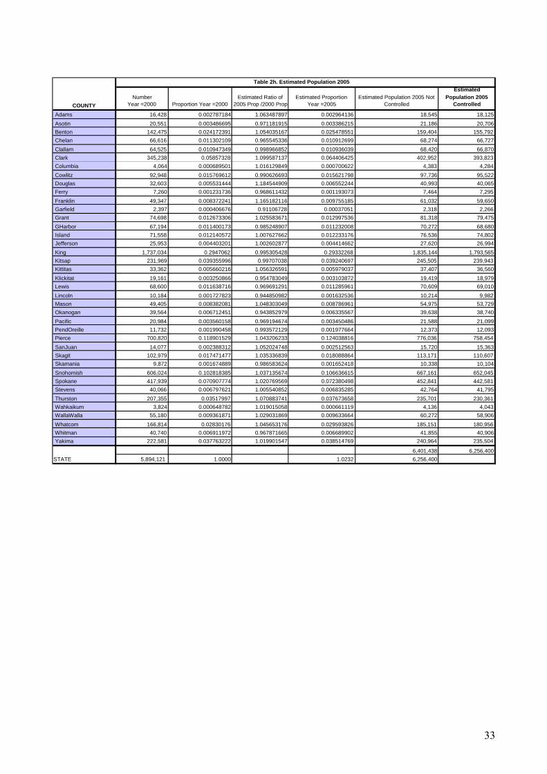
Number Year =2000 Proportion Year =2000

Estimated Ratio of2005 Prop /2000 Prop

Estimated Proportion Year =2005

Estimated Population 2005 Not Controlled

Estimated Population 2005

Controlled

Adams 16,428 0.002787184 1.063487897 0.002964136 18,545 18,125 Asotin 20,551 0.003486695 0.971181915 0.003386215 21,186 20,706 Benton 142,475 0.024172391 1.054035167 0.025478551 159,404 155,792 Chelan 66,616 0.011302109 0.965545336 0.010912699 68,274 66,727 Clallam 64,525 0.010947349 0.998966852 0.010936039 68,420 66,870 Clark 345,238 0.05857328 1.099587137 0.064406425 402,952 393,823 Columbia 4,064 0.000689501 1.016129849 0.000700622 4,383 4,284 Cowlitz 92,948 0.015769612 0.990626693 0.015621798 97,736 95,522 Douglas 32,603 0.005531444 1.184544909 0.006552244 40,993 40,065 Ferry 7,260 0.001231736 0.968611432 0.001193073 7,464 7,295 Franklin 49,347 0.008372241 1.165182116 0.009755185 61,032 59,650 Garfield 2,397 0.000406676 0.91106728 0.00037051 2,318 2,266 Grant 74,698 0.012673306 1.025583671 0.012997536 81,318 79,475 GHarbor 67,194 0.011400173 0.985248907 0.011232008 70,272 68,680 Island 71,558 0.012140572 1.007627662 0.012233176 76,536 74,802 Jefferson 25,953 0.004403201 1.002602877 0.004414662 27,620 26,994 King 1,737,034 0.2947062 0.995305428 0.29332268 1,835,144 1,793,565 Kitsap 231,969 0.039355996 0.99707038 0.039240697 245,505 239,943 Kittitas 33,362 0.005660216 1.056326591 0.005979037 37,407 36,560 Klickitat 19,161 0.003250866 0.954783049 0.003103872 19,419 18,979 Lewis 68,600 0.011638716 0.969691291 0.011285961 70,609 69,010 Lincoln 10,184 0.001727823 0.944850982 0.001632536 10,214 9,982 Mason 49,405 0.008382081 1.048303049 0.008786961 54,975 53,729 Okanogan 39,564 0.006712451 0.943852979 0.006335567 39,638 38,740 Pacific 20,984 0.003560158 0.969194674 0.003450486 21,588 21,099 PendOreille 11,732 0.001990458 0.993572129 0.001977664 12,373 12,093 Pierce 700,820 0.118901529 1.043206233 0.124038816 776,036 758,454 SanJuan 14,077 0.002388312 1.052024748 0.002512563 15,720 15,363 Skagit 102,979 0.017471477 1.035336839 0.018088864 113,171 110,607 Skamania 9,872 0.001674889 0.986583624 0.001652418 10,338 10,104 Snohomish 606,024 0.102818385 1.037135674 0.106636615 667,161 652,045 Spokane 417,939 0.070907774 1.020769569 0.072380498 452,841 442,581 Stevens 40,066 0.006797621 1.005540852 0.006835285 42,764 41,795 Thurston 207,355 0.03517997 1.070883741 0.037673658 235,701 230,361 Wahkaikum 3,824 0.000648782 1.019015058 0.000661119 4,136 4,043 WallaWalla 55,180 0.009361871 1.029031869 0.009633664 60,272 58,906 Whatcom 166,814 0.02830176 1.045653176 0.029593826 185,151 180,956 Whitman 40,740 0.006911972 0.967871665 0.006689902 41,855 40,906 Yakima 222,581 0.037763222 1.019901547 0.038514769 240,964 235,504

6,401,438 6,256,400

STATE 5,894,121 1.0000 1.0232 6,256,400

COUNTY

Table 2h. Estimated Population 2005