On the quest for chaotic attractors in hydrological processes · On the quest for chaotic attractors in hydrological processes ... in some cases, merely the careful application of

Hydrological Sciences–Journal–des Sciences Hydrologiques, 51(6) December 2006

Open for discussion until 1 June 2007 Copyright © 2006 IAHS Press

1065

On the quest for chaotic attractors in hydrological processes DEMETRIS KOUTSOYIANNIS Department of Water Resources, Faculty of Civil Engineering, National Technical University of Athens, Heroon Polytechneiou 5, GR-157 80 Zographou, Greece [email protected] Abstract In the last two decades, several researchers have claimed to have discovered low-dimensional determinism in hydrological processes, such as rainfall and runoff, using methods of chaotic analysis. However, such results have been criticized by others. In an attempt to offer additional insights into this discussion, it is shown here that, in some cases, merely the careful application of concepts of dynamical systems, without doing any calculation, provides strong indications that hydrological processes cannot be (low-dimensional) deterministic chaotic. Furthermore, it is shown that specific peculiarities of hydrological processes on fine time scales, such as asymmetric, J-shaped distribution functions, inter-mittency, and high autocorrelations, are synergistic factors that can lead to misleading conclusions regarding the presence of (low-dimensional) deterministic chaos. In addition, the recovery of a hypo-thetical attractor from a time series is put as a statistical estimation problem whose study allows, among others, quantification of the required sample size; this appears to be so huge that it prohibits any accurate estimation, even with the largest available hydrological records. All these arguments are demonstrated using appropriately synthesized theoretical examples. Finally, in light of the theoretical analyses and arguments, typical real-world hydrometeorological time series, such as relative humidity, rainfall, and runoff, are explored and none of them is found to indicate the presence of chaos. Keywords attractors; capacity dimension, chaos; chaotic dynamics; correlation dimension; entropy; hydrological processes; nonlinear analysis; stochastic processes; time series analysis; rainfall; runoff

Sur la recherche d’attracteurs chaotiques dans des processus hydrologiques Résumé Durant les deux dernières décennies, plusieurs chercheurs ont prétendu avoir découvert le déterminisme bas dimensionnel dans des processus hydrologiques, tels que les précipitations et l'écoulement, en utilisant des méthodes d'analyse chaotique. De tels résultats, cependant, ont été critiqués par d'autres. Afin d'essayer d'offrir des avis supplémentaires dans cette discussion, on montre ici que, dans certains cas, la simple application soigneuse des concepts des systèmes dynamiques, sans aucun calcul, fournit de fortes indications que les processus hydrologiques ne peuvent pas être chaotiques déterministes (bas dimensionnels). En outre, on montre que les particularités spécifiques des processus hydrologiques aux échelles temporelles fines, telles que l'asymétrie, les fonctions de distribution en forme de J, l’intermittence et les autocorrélations élevées, sont des facteurs synergiques qui peuvent mener à des conclusions fallacieuses concernant la présence du chaos déterministe (bas dimensionnel). En outre l’identification d'un attracteur hypothétique à partir d'une série chronologique est posée comme un problème statistique d'estimation, dont l'étude permet, entre d'autres, la quantification de la taille requise de la série; celle-ci apparaît être si grande qu'elle interdit toute estimation précise, même avec les plus longues séries hydrologiques disponibles. Tous ces arguments sont démontrés en utilisant des exemples théoriques convenablement synthétisés. En conclusion, à la lumière de nos analyses et arguments théoriques, des séries chronologiques hydrométéorologiques réelles typiques, telles que de l'humidité relative de l’air, de la précipitation et de l'écoulement, sont explorées et aucune d'elles ne se révèle être indicatrice de la présence de chaos. Mots clefs attracteurs; dimension de capacité; chaos; dynamique chaotique; dimension de corrélation; entropie; processus hydrologiques; analyse nonlinéaire; processus stochastiques; analyse de séries temporelles; pluie; écoulement INTRODUCTION “My thirteenth and last thesis is this. Both classical physics and quantum physics are indeterministic.” Karl Popper (in his book Quantum Theory and the Schism in Physics, Routledge, 1992) The impressive results of chaos analysis of simple physical and mathematical systems in the last two decades offered an alternative way to view natural systems. Specifically, it became clear that a simple nonlinear deterministic system, even with one degree of

Demetris Koutsoyiannis

Copyright © 2006 IAHS Press

1066

freedom, can have a complex, random-appearing evolution. Obviously, however, the inverse is not true: complex or erratic-appearing phenomena do not necessarily imply that the dynamics are simple. Loosely speaking, the complexity of a system with deterministic dynamics depends on the number of degrees of freedom, or dimension of the system attractor, and on how many of them are associated with sensitive dependence on initial condi-tions. The latter are quantified by positive values of the so called Lyapunov exponents that are associated with the system dynamics. Chaotic systems are in fact the simplest possible deterministic systems with sensitivity to initial conditions: those that have one positive Lyapunov exponent (Kantz & Schreiber, 1997, pp. 183, 241), and typically have attractor dimension less than two (Kantz & Schreiber, 1997, p. 183). Following Kantz and Schreiber, in this paper, the term “low-dimensional (deterministic) chaos” is used as synonymous to chaos (even though, as correctly pointed out by Schertzer et al., 2002, initially the word chaos was used to describe stochastic phenomena such as Brownian motion, or any kind of disorder—cf. Greek mythology). Systems with very many (theoretically infinite) dimensions are usually (and in this paper too) characterized as stochastic (or random) systems and are usually modelled using probabilistic considerations and the theory of stochastic processes. In a stochastic system, the future of the system state cannot be determined completely from its present and past, even if the entire past is known. However, the characterization of a system as a stochastic (or a random) system should not be regarded as the denial of deterministic dynamics in its evolution, but rather as the inadequacy or inefficiency of a pure deter-ministic mathematical description. For example, tossing of dice is regarded as the most typical example of a random system (cf. Albert Einstein’s famous aphorism), even though its outcome depends on a few collisions of a cube onto a plane, whose deter-ministic dynamics can be understood rather easily (perhaps more easily than those of a hydrological system also influenced by the global circulation system). Perhaps to fill the gap between the very low-dimensional chaotic systems and the very high-dimensional stochastic systems, the term hyperchaos has been coined (Rössler, 1979; Kantz & Schreiber, 1997, pp. 183, 241). While numerous chaotic and stochastic systems have been studied thoroughly, only a few experimental observations of hyperchaos have been recorded. To explain this lack of higher dimensional experi-mental attractors, Kantz & Schreiber offer two possible explanations: typical systems in nature possess either exactly one or very many positive Lyapunof exponents; or systems with a higher-than-three-dimensional (3D) attractor are very difficult to analyse. Traditionally, stochastic models have been the preferred mathematical tools in hydrology and water resources modelling. Hydrological processes have been most frequently modelled as stochastic processes, which also incorporate apparent determin-istic components of the natural processes (e.g. periodicity) in addition to random components. However, in the last two decades, the charming possibility that a complex hydrological system with irregular time evolution may au fond be a simple chaotic system has motivated several researchers to analyse hydrological processes using mathematical tools of the chaos literature. Their intention and hope, perhaps, was to discover simplicity and universal determinism in place of what was earlier considered as stochastic behaviour with weak deterministic imprints. Thus, an increasing number of studies have tried to show that hydrological processes are chaotic. Sivakumar (2000, 2004) reviews most of the studies related to chaotic analysis of hydrological processes.

On the quest for chaotic attractors in hydrological processes


1067

Such studies, whose number has continuously increased since the late 1980s, have analysed processes such as rainfall, runoff and lake storage using time series with resolutions from a few seconds to one month and data sizes from one to several thousands. In most cases, the authors claimed that they discovered deterministic attractors with dimensions varying from about 1/2 to about 10. Few authors reported absence of chaos or expressed scepticism about the discovery of chaos in other studies and provided arguments for the incorrectness of such results. The attempts to discover chaos in natural phenomena are not unique to hydrology. As pointed out by Provenzale et al. (1992), “… the desire for finding a chaotic attractor has led to a naïve application of the analysis methods; as a result, the number of claims on the presence of strange attractors in vastly different physical, chemical, biological and astronomical systems has grown (exponentially?)”. Here they quote a statement by Grassberger et al. (1991): “… most (if not all) of these claims have to be taken with much caution”. They also note that convincing evidence for chaos most commonly arises when spatial complexity of the system is limited, a condition that could be true for experimental systems, but is far from true for hydrological and other geophysical processes. The present paper attempts to proceed a step further than simply expressing scepticism about the discovery of chaos in hydrological processes. Specifically, it endeavours to show that the hypothesis that hydrological time series manifest stochastic, rather than chaotic, systems cannot be rejected using the standard pro-cedures of chaotic analysis. In addition, it locates critical issues that may lead to an erroneous conclusion that a hydrological system is chaotic; such issues may have influenced earlier studies that identified chaos in hydrology. Here, it should be made clear that the intent of the paper is not to spot flaws or erroneous conclusions in particular earlier studies. This is the reason why specific references to these studies (or to studies that expressed scepticism) are deliberately avoided. The references included are only those that describe theoretical developments or methodologies used in this paper. The interested reader is referred to the comprehensive reviews by Sivakumar (2000, 2004) for locating related studies and to Sivakumar et al. (2001, 2002) and Schertzer et al. (2002) for one of the most recent debates on the issue. In addition to identifying the critical issues, the paper develops ways to recover from them and draw correct conclusions. To this aim, the paper first briefly reviews some fundamental concepts of chaotic behaviour and the typical procedure for identi-fying chaos based on the estimation of attractor dimensions; it is the author’s opinion that revisiting fundamental concepts is generally useful, and necessary for the particu-lar scope of this paper. Subsequently, the paper shows that, in some cases, merely the careful application of the concepts of dynamical systems provides strong indications that hydrological processes cannot be chaotic. Furthermore, it shows that peculiarities of hydrological processes can lead to misleading conclusions regarding presence of chaos, and in addition demand huge data sets, whose size can be quantified by statistical reasoning. Finally, in light of the theoretical analyses and arguments, typical real-world hydrometeorological time series are explored and none of them is found to indicate the presence of chaos. Details of the real-world examples as well as mathe-matical derivations that support the theoretical analysis are given separately in Koutsoyiannis (2006).



1068

The scope of this paper cannot include all of the numerous applications of chaotic tools in hydrology. For instance, many studies have used nonlinear forecast methods from chaotic dynamical systems in hydrological applications. The success of such applications is not in question, but, as strange as it may seem, this does not necessarily indicate that the system at hand is chaotic. For example, in a recent study (Koutsoyiannis et al., 2006), a low-dimensional chaotic nonlinear method gave fore-casts of the monthly flow of the Nile that were equally good in the case that the inflows were historical or synthetic (generated by a stochastic model). Thus, the scope here is limited to identification of potential chaos and for this reason the emphasis is given to time delay embedding of attractors, which has been the standard method for identification of chaos both in general and in hydrological applications. DESCRIPTORS OF CHAOTIC BEHAVIOUR Dynamical systems and attractors The nonlinear time series methods which are applied in hydrology are based on the theory of dynamical systems; these are characterized by: (a) a phase or state space in which the motion of the system takes place; (b) a rule stating where to go next from the current system position (also known as system dynamics); and (c) a time set that describes the moments at which movements from one position to another take place. Typically, the phase space M is a finite-dimensional vector space Rm and the state of the system is specified by a vector x with size m. The time set is typically either the set of integers I (discrete time) or the set of real numbers R (continuous time). The system dynamics is a family of transformations St: M → M (where t denotes time) satisfying (Lasota & Mackey, 1994, p. 191):

S0(x) = x St(St΄(x)) = St + t΄(x) x ∈ M (1)

In discrete time, the system dynamics is completely determined by the m-dimensional map S1:

xn+1 = S1(xn) n ∈ I (2)

In continuous time the dynamics is described as a system of m ordinary differential equations:

dx(t)dt = s(x(t)) t ∈ R (3)

whose solution defines the family of transformations St. For a given initial point x0 or x(0), the sequence of points xn = Sn(x0) or the function x(t) = St(x(0)) considered as a function of n or t is called a trajectory of the dynamical system. In the so-called dissipative dynamical systems, the trajectory of the system, after some transient time, is attracted to some subset A of the phase space. This set itself is invariant under the dynamical evolution (St(A) = A) and is called the attractor of the system (Kantz & Schreiber, 1997, p. 32). Only three types of attractors can occur (e.g. Lasota & Mackey, 1994, p. 192; Kantz & Schreiber, 1997, p. 32): (a) fixed points indicating that the system settles to a stagnant state, i.e. xn = x0 or St(x(0)) = x(0), for all n or t; (b) limit cycles, indicating periodic motion with period ω,



1069

i.e. xn+ω = xn or St+ω(x(0)) = St(x(0)), for all n or t; and (c) non-intersecting trajectories, in which case xn1

≠ xn2 or St1(x(0)) ≠ St2(x(0)), for all n1 ≠ n2 or t1 ≠ t2. For a system in

continuous time with a two-dimensional (2D) state space, the fixed point and cycle are the only possibilities, whereas for three dimensions and beyond, the more interesting non-intersecting attractors can occur, which typically exhibit fractal structure and are called strange attractors. For systems in discrete time the non-intersecting attractors can occur even in a 2D state space (Lasota & Mackey, 1994). Delay embedding and reconstruction of dynamics In this paper, as in other hydrological applications of chaotic dynamics, only systems expressed in terms of a single scalar real quantity y (e.g. rainfall, runoff, etc.) are considered. Such a system evolves in continuous time, and its m-dimensional state x is theoretically expressed in terms of the quantity y and a number m – 1 of its derivatives with respect to time, i.e. x(t) := [y(t), y΄(t), … y(m-1) (t)]T (where (y(k) := dky/dyk and the superscript T denotes the transpose of a vector or matrix). However, in a hydrological (natural) system, only observations of the quantity y on discrete time intervals Δt (and no observations of its derivatives) can be available. Therefore, the study of the system is done as if it were a discrete time system using the so-called delay vectors:

xn := [yn, yn-τ, …, yn-(m-1)τ]T (4)

where yn := y(nΔt) and τ is a positive integer. By studying the simplified discrete time system, the properties of the original system since can be inferred. According to Takens’ embedding theorem (Takens, 1981), for properly chosen embedding dimen-sion m and time delay τ, the discrete time system will trace out a trajectory that represents a smooth coordinate transformation of the original trajectory of the system. Thus, the Takens theorem allows for the reconstruction of the dynamics of the system using a time series of a single scalar observable. If the only given information is the time series, it is not known a priori what the proper embedding dimension m is. This dimension depends on the dimension D of the attractor. The latter dimension has important content as D (or better the smallest integer that is not smaller than D) represents the number of degrees of freedom needed to describe the state of the system (Gershenfeld & Weigend, 1993, p. 48). According to Whitney’s (1936) embedding theorem, which was generalized for fractal objects by Sauer et al. (1991), any D-dimensional object (precisely, any D-dimensional smooth manifold) can be embedded in an m-dimensional Euclidean space if m > 2D. For example, a one-dimensional curve of any shape can always be embedded in a 3D Euclidean space (and all higher-dimensional spaces), but it cannot be embedded in a 2D space because, except for special cases, it will overlap itself (this will be further clarified later). Thus, an attractor of the non-intersecting type with dimension 1 will intersect itself in a 2D space (projection) but not in a 3D space. Therefore, if the attractor dimension D were known, the state vector size m would be the smallest integer that is greater than 2D. But since D is unknown when merely a time series is available, an iterative procedure is followed. For trial m = 1, 2, …, the dimension D(m) of the trajectory of the system is estimated at the m-dimensional



1070

space, until D(m) becomes constant with the further increase of m. This constant is the attractor dimension. Estimation of dimensions The problem arises then of how to estimate the dimension D of a trajectory or attractor A in an m-dimensional vector space. The estimate of a dimension is typically done in terms of entropic quantities. It should be stressed that entropy is a probabilistic concept and thus the estimation of entropic quantities obeys statistical laws (although in some studies this is missing). Specifically, let A be a subset of an m-dimensional metric space with a normalized measure P( ) defined on its Borel field. Equivalently, A can be regarded as a sample space and the normalized measure P(B) of any subset B of A as the probability of B. In our case, for m = 1, A may represent all possible values of a hydrological variable such as rainfall or runoff at a specified time scale, so that it is the set of positive real numbers R+. Accordingly, for m > 1, the set may represent the m-dimensional space formed by the delay vectors. Let us consider a partition of A into ν(ε) boxes (hypercubes) A1, A2, …, Aν(ε) with scale length (or simply scale, meaning edge length of each hypercube) ε. The standard entropy, also known as the information entropy or the Boltzmann-Gibbs-Shannon entropy is by definition:

φ(ε) := – ∑i=1

ν(ε) pi ln pi (5)

where pi := P(Ai) is the measure of the part of the set A contained in the ith hypercube having the obvious property:

∑i=1

ν(ε) pi = 1 (6)

Equivalently, pi could be interpreted as the probability that a point of A belongs to Ai. In this case, φ(ε) is the expected value of the minus logarithm of probability (in this case meant on the specific partition) and is typically interpreted as a measure of uncertainty. Several generalizations of the standard entropy have been proposed (Rényi, 1970; Tsallis, 2004). Among them, the most commonly used for the identification of chaotic systems is the Rényi entropy of order q defined to be:

φq(ε) := 1

1 – q ln ∑i=1

ν(ε) pq

i (7)

Application of de l’ Hôpital’s rule to equation (7) for q = 1 shows that φ1(ε) ≡ φ(ε). The entropy φq(ε) is a decreasing function of ε and tends to infinity as ε tends to zero. However, the quantity

Dq :=

limε→0

–φq(ε)

ln ε (8)



1071

takes a finite value and it is called the generalized dimension of order q of the set and normalized measure under examination (Grassberger, 1983). Applying de l’Hôpital’s rule in equation (8), one obtains:

Dq =

limε→0

d(–φq(ε))

d(ln ε) (9)

The latter expression is more advantageous than equation (8) for numerical applica-tions, since the convergence of the derivative is faster. For low values of q, the most frequently used dimensions are produced. Thus, q = 0 gives the so-called “box counting” or “capacity” dimension D0, q = 1 the “information” dimension D1, and q = 2 the “correlation” dimension D2. For simple geometrical objects such as segments of a line or a surface, if the Lebesgue measure is used (equivalently, if the uniform probability distribution is assumed) then all Dq are equal to the integer topological dimension (1 for a line, 2 for a surface, etc.). For more complex mathematical objects including fractal objects or for these simple objects but for other measures (or probability distributions), they are not necessarily integers, nor all Dq are necessarily equal to each other, as will be demonstrated later. The most important among generalized dimensions is the capacity dimension D0, because this is in fact the one used in the extension by Sauer et al. (1991) of Whitney’s (1936) embedding theorem mentioned above. However, the most frequently used (for reasons that will be explained next) is the correlation dimension D2. Estimates of probabilities and entropic quantities can be derived by statistical theory based on a certain observed time series or delay vectors thereof. Thus, the statistical estimate of pi from a sample of N observed values, each one denoted as xj (or a vector sample of N points in the m-dimensional space that is formed by time delay vectors, each one denoted as xj), of which Ni are contained in the ith hypercube Ai, is typically derived as pi = Ni/N. Accordingly, the estimates of dimensions can be derived by numerical evaluation of equations (5)–(9), substituting Ni/N for pi. For integer q ≥ 2, an alternative estimation can be done in terms of the so-called generalized correlation sum of order q, introduced by Grassberger (1983):

Cq(ε) := {fraction of q-tuples (xj1, …, xjq) that have all ||xjs − xjr|| < ε} (10)

where ||.|| denotes the norm of a vector. This has the important property:

Cq(ε) ≈ exp[(1 – q) φq(ε)] (11)

Thus, for integer q ≥ 2, –φq(ε) can be replaced with ln Cq(ε)/(q – 1) in the calculation of dimensions using the above equations; the estimation of φq(ε) in terms of Cq(ε) is regarded as more accurate than that in terms of Ni/N (Grassberger, 1983; Grassberger & Procaccia, 1983). In practice however, only the correlation sum for q = 2 is used, because the calculation of higher-order sums is very time consuming. (In fact, this is the case even for q = 2.) The correlation sum of order 2, or simply the correlation sum, is given by the following equation that is a consequence of equation (10):

C2(ε, m) = 2

(N – w) (N – w + 1) ∑i=1

N–w ∑j=i+w

N H(ε – ||xi – xj||) (12)

where H is the Heaviside step function, with H(u) = 1 for u > 0 and H(u) = 0 for u ≤ 0,



1072

and w is an integer constant, which for uncorrelated time series is assumed one but for correlated ones may be assigned a greater value to exclude from the estimation those pairs of points that are close in time (Kantz & Schreiber, 1997, p. 74). For the calculation of the distance ||xi – xj||, the maximum norm is usually used as it reduces the computa-tional time (Hübner et al., 1993). The seemingly complex formula (12) should not prevent one to see that the correlation sum C2(ε, m) is the proportion of pairs of points having distance smaller than ε between them. In other words, the correlation sum C2(ε, m) is the estimate of the true (population) probability that the distance of any two points is smaller than ε. Typical procedure for identifying chaos The estimation procedure of the correlation dimension D2 in terms of correlation sums, known as the Grassberger-Procaccia algorithm (after Grassberger & Procaccia, 1983) consists of the following steps: 1. Calculate the correlation sum C2(ε, m) for several values of the scale ε. 2. Make a log-log plot of C2(ε, m) vs ε and a plot of the local slope d2(ε, m) vs logε,

where:

d2(ε, m) := Δ[ln C2(ε, m)]

Δ[ln ε] (13)

and locate a region with constant slope, known as a scaling region (e.g. Hübner et al., 1993).

3. Calculate the slope of the scaling region, which is the estimate of the correlation dimension D2(m) of the set for the embedding dimension m.

As explained above this is done iteratively for m = 1, 2, … and iterations stop when D2(m) saturates to a constant value D2, independent of m. The convergence of D2(m) to the value D2 verifies that a D2-dimensional attractor: (a) exists, which means that the system under study is deterministic; (b) has been identified; and (c) can been embedded in an m-dimensional space where m is the minimum integer for which D2(m) = D2. Conversely, if D2(m) does not become constant for increasing m, the system is characterized as stochastic, rather than deterministic. This procedure has been followed in most of the hydrological applications mentioned in the introduction to characterize a time series as stochastic or deterministic. Several authors have warned that the procedure has several critical points that require careful attention (see discussions in, among others, Tsonis, 1992; Tsonis et al., 1993; Kantz & Schreiber, 1997; Graf von Hardenberg, 1997a; Sivakumar, 2000), otherwise the results may be flawed. These points are revisited in the next section, and some additional critical points whose ignorance could result in erroneous interpretations are introduced. IMPORTANT ISSUES IN IDENTIFYING CHAOS IN HYDROLOGICAL PROCESSES A conceptual approach to the dimensionality of a hydrological attractor Before applying any algorithm to quantify the dimensionality of an attractor in a hydrological process, it would be a good idea to try a more conceptual approach and to



1073

determine, if possible, what would be a reasonable expectation of this dimensionality. It is natural to start with the rainfall process in discrete time on daily time scale (the same reasoning applies in finer time scales as well). For this process and time scale some studies have claimed to have seen chaos with dimensionality D2 as low as 1 (or less). In a daily rainfall time series there exist periods with zero rainfall. Let us consider here the complete time series with consecutive dry and wet periods, similar to what most studies have done. (Later fine time scale rainfall series excluding dry periods will be also examined). Let k be the maximum observed dry period in days. For example, in Athens, Greece, in a 132-year record of rainfall record, k = 130 days (more than four months). The day when this dry period starts is set n = 1, so that the rainfall depths yn for n = 1 to k are all zero. Let us assume that the rainfall at the examined location is the outcome of a deterministic system whose attractor can be embedded in Rm for some integer m. This attractor is reconstructed using delay embedding with delay τ. Further-more, let us assume that m < (k – 1)/τ + 1. Then, there exist at least two delay vectors with all their components equal to zero. Namely, xk = [yk, yk–τ , yk–2τ , …, yk–(m–1)τ ]T = 0 and xk-1 = [yk-1, yk-1-τ, yk-1-2τ, …, yk-1-(m-1)τ]T = 0 where 0 is the zero vector. Therefore, xk = S1(xk-1) = S1(0) = 0, and since the system is deterministic, it will result in xn = 0 for any n > 0 (since xk+1 = S1(xk) = S1(0) = 0, etc.). That is, given that rainfall is zero for a period k, it will be zero forever, which means that the attractor is a single point. This of course is absurd and thus the embedding dimension should be m ≥ (k – 1)/τ + 1. Now, Whitney’s embedding theorem (Kantz & Schreiber, 1997, p. 126) tells us that the attractor should have dimension D ≥ (m – 1)/2 and, hence, D ≥ (k – 1)/2τ. For example (as in Athens), if the maximum dry period k = 130 and a “safe” delay τ = 10 is assumed (this will be discussed further later), the above analysis results in an embedding dimension of at least 13 and an attractor dimension of at least 6. As high as this attractor dimension may seem (compared to values reported in some hydrological applications), it is still too low. In this reasoning, rainfall has been considered as a discrete time process. If it were considered as a continuous time process, as in fact is, then instead of assuming x as a vector of delay coordinates, it would be regarded as x(t) = [y(t), y΄(t), … y(m-1)t)]T, as explained earlier. Now, at any time within a dry period, x(t) = 0, regardless of the dimension m used (the rainfall depth and all its derivatives of any order are zero). Clearly then, the attractor cannot be of the non-intersecting type (since x(t) = 0 for several, in fact infinite, values of t), but it will be of the fixed-point type, the fixed point being the zero vector. Of course, this is not true, because at some time the system will depart from the “attracting” zero point. Thus, the system that is described by the rainfall depth is not low-dimensional (it cannot have a finite dimensional attractor), but rather infinite-dimensional (stochastic). On coarser discrete time scales, such as monthly, it may be the case (for wet areas) that the zero rainfall values do not occur. However, if the rainfall process is high- or infinite-dimensional on fine time scales, naturally it will be high- or infinite-dimensional on coarser time scales as well. In addition, since rainfall is the input that mobilizes all other hydrological processes in a catchment, the number of degrees of freedom of any other hydrological process (e.g. streamflow) will be at least equal to that of rainfall. Moreover, if rainfall is indeed stochastic, all other processes in the catchment will also be stochastic.



1074

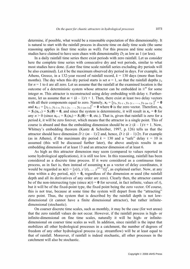
Until now, the conceptual approach followed did not use any algorithm at all. In the case of application of an algorithm, it could be a good idea to examine whether its results are conceptually consistent and meaningful. For example, if the attractor dimen-sion were found to be as low as one or even smaller, as indeed happens in some of the applications published, then it would have a direct geometrical interpretation. To demonstrate what an attractor with dimension one or less looks like, an example from a system with known chaotic dynamics was constructed. The well-known logistic equa-tion zn = a zn-1(1 – zn-1) with a = 3.97977, which obviously has one degree of freedom (so that D ≤ 1), was used as a starting point. Then, to make the attractor more interesting, zn was routed through a linear filter to obtain the series yn := b0 zn + b1 zn-1 + b2 zn-2 + b3 zn-3 + b4 zn-4 with b0 = 1, b1 = 2, b2 = 1.5, b3 = 1, b4 = 0.5. Here, no additional degree of freedom was introduced and thus the dimension of the attractor was not increased; this was verified using the Grassberger-Procaccia algorithm. The attractor, constructed graphically using 10 000 points, is shown in Fig. 1 in a 2D (upper panel) and a 3D (lower panel) space. That the dimension of the attractor does not exceed one is obvious in both panels, although the 2D graph is not appropriate to show the non-intersecting type of the attractor (it intersects itself). Now if the same work is done with a hydrological series, a totally different picture is obtained. In Fig. 2, an “attractor” has been plotted in a 2D (upper panel) and a 3D (lower panel) space using 10 000 points of a daily rainfall series, which will be discussed further in the section “Real world examples”. These graphs are typical for any daily rainfall series. One cannot locate any one-dimensional structure in such graphs. On the contrary, the cloud of points fills all space both in two and three dimensions. Therefore its topological dimension, which is expressed by the capacity dimension D0, equals the embedding dimension, that is, 2 in the upper panel and 3 in the lower panel. As will be shown in the next sub-section, the correlation dimension of this 2- or 3-dimensional space filling cloud could be 1 or even less, but this is totally irrelevant. What matters is that the cloud of points fills up space and, thus, the capacity dimension equals the embedding dimension. One may argue that the plots of Fig. 2 are in two and three dimensions, whereas studies that estimated attractor dimensions of the order of one have simultaneously shown that the embedding dimension should be at least 10 or more, possibly up to 40. But clearly this is an inconsistency of these studies. If the attractor dimension were one or less, then, according to Whitney’s embedding theorem, a 3D embedding space would suffice to embed it (there would be no need to go to embedding dimensions 10–40). Another type of suspect results are those in which runoff appears to have an attractor with dimension lower than that of rainfall at the same area and time scales. As explained above, it is difficult to imagine how runoff (hydrological system output) could have dimension smaller than rainfall (hydrological system input). Capacity vs correlation dimension and the effect of an asymmetric distribution Wang & Gan (1998) have pointed out that the underlying distribution function plays a role in the estimation of correlation dimension. They demonstrated this by using random data series generated from Gamma and Poisson distributions. They argued that



1075

1.5

2.0

2.5

3.0

3.5

4.0

4.5

5.0

1.5 2.0 2.5 3.0 3.5 4.0 4.5 5.0

y t - 1

y t

yt - 1

yt - 2

y t

Fig. 1 Delay representation of a series of 10 000 points generated from the linearly routed logistic equation (see text) in two (upper panel) and three (lower panel) dimensions.

the correlation dimension for these data series is underestimated due to a clustering feature, or an “edging effect”. In this section, this issue is analysed theoretically and it is shown that small estimated values of correlation dimension should not necessarily be interpreted as underestimated, as in fact can be correct estimates—but these estimates are irrelevant to the existence of an attractor. It can be easily shown that, in random time series from a continuous distribution function, the capacity dimension D0(m) equals the embedding dimension, m, or, in other words, the time-delayed vectors fill up the embedding space. This has been given a key role in identifying chaos in hydrological processes and particularly in the charac-terization of a process of chaotic rather than stochastic. However, as discussed in the



1076

0

20

40

60

80

100

0 20 40 60 80 100

yt - 1

y t

yt - 1

yt - 2

y t

Fig. 2 Delay representation of a series of 10 000 daily rainfall depths in two (upper panel) and three (lower panel) dimensions.

section “Descriptors of chaotic behaviour”, in identifying chaos the correlation dimen-sion D2(m) rather than the capacity dimension D0(m) has been typically used. It is the rule that the correlation dimension of a random series D2(m) equals D0(m) and therefore the embedding dimension m. It is shown (Koutsoyiannis, 2006) that a sufficient condition for this rule to be valid is that the probability density functions f(y) is square-integrable, i.e.

⌡⌠A

f 2(y)dy < ∞ (14)

Furthermore, it is shown that this condition may be not valid in purely random processes following non-symmetric J-shaped distributions, for which D2(m) is smaller than m. More specifically, it is shown that in such processes and for embedding dimension m = 1:



1077

D2(1) = 2 + 2

limε→0

ε f ΄(ε)

f(ε) < 1 = D0(1) (15)

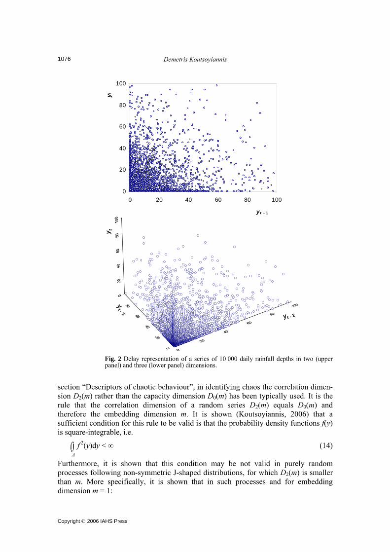
where f ΄( ) is the derivative of f( ). By analogy, D2(m) = mD2(1) < m (but D0(m) = m). For example, it was shown (Koutsoyiannis, 2006) that in distribution functions typically used in hydrology, such as Pareto, Gamma and Weibull, with shape parameter κ smaller than 1/2 or, equivalently, coefficients of skewness greater than 0.639, 2.83 and 6.62, respectively, the correlation dimension for embedding dimension 1 is D2(1) = 2κ < 1. A demonstration of this is given in Fig. 3 using a series of 10 000 random points generated from the Pareto distribution F(y) = yκ, 0 ≤ y ≤ 1 with shape parameter κ = 1/8. Here it is expected that D2(m) = 0.25 m. In Fig. 3, the estimated correlation sums C2(ε, m) (upper panel) and their local slopes d2(ε, m) (lower panel) have been plotted vs scale ε for embedding dimensions m = 1 to 8. It should be noted

1E-08

1E-07

1E-06

1E-05

1E-04

1E-03

1E-02

1E-01

1E+00

1E-06 1E-05 1E-04 1E-03 1E-02 1E-01 1E+00ε

C2(ε,

m)

1 2 3 45 6 7 8

0

0.5

1

1.5

2

2.5

3

3.5

4

1E-06 1E-05 1E-04 1E-03 1E-02 1E-01 1E+00ε

d2(ε,

m)

1 2 3 45 6 7 8

ε_

ε 1

Fig. 3 Correlation sums C2(ε, m) (upper panel) and their local slopes d2(ε, m) (lower panel) vs scale ε for embedding dimensions m = 1 to 8 calculated from a series of 10 000 independent random values with Pareto distribution with exponent 1/8.



1078

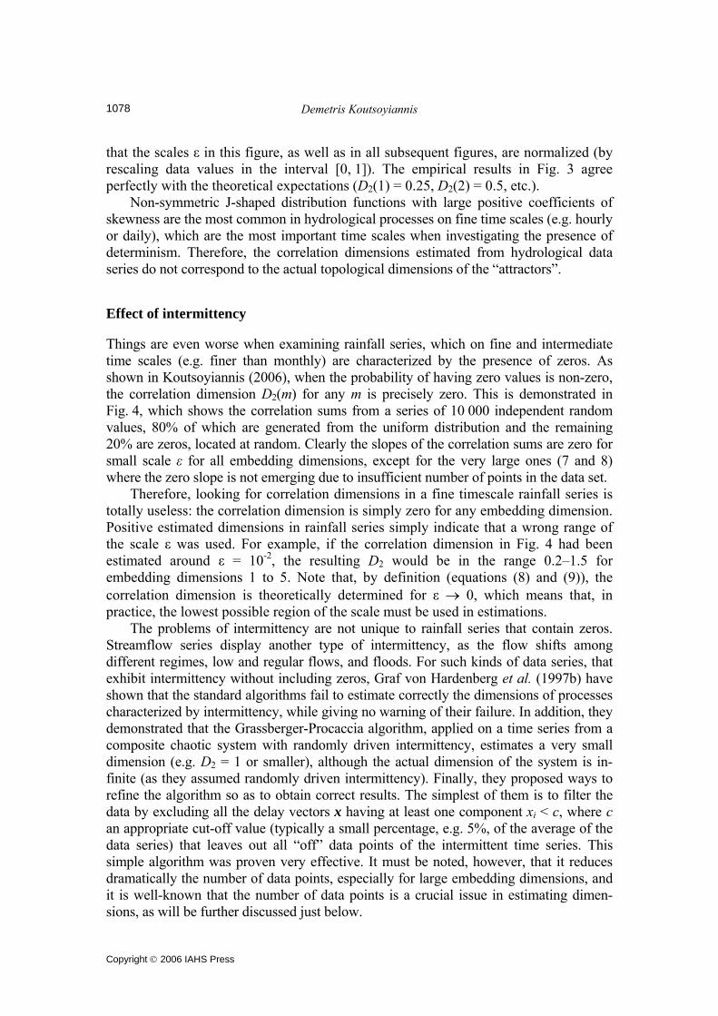
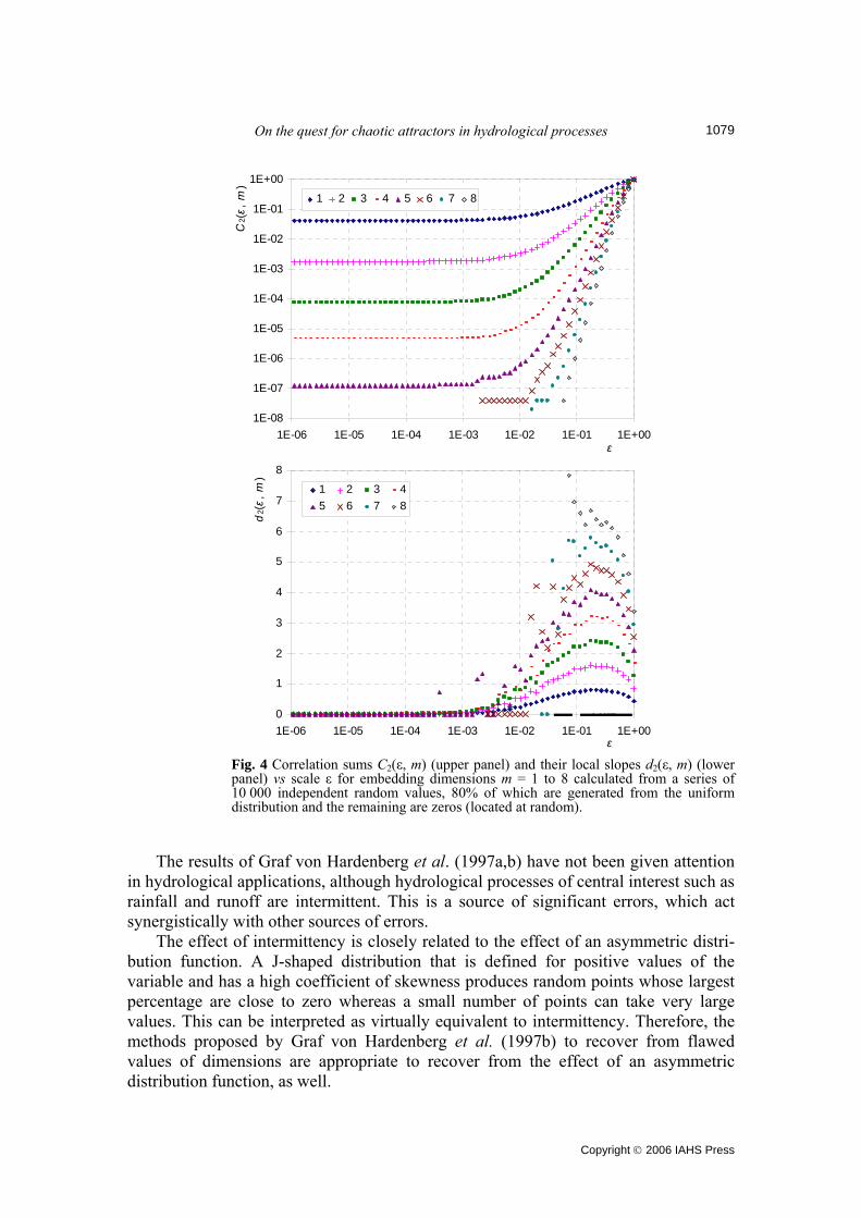
that the scales ε in this figure, as well as in all subsequent figures, are normalized (by rescaling data values in the interval [0, 1]). The empirical results in Fig. 3 agree perfectly with the theoretical expectations (D2(1) = 0.25, D2(2) = 0.5, etc.). Non-symmetric J-shaped distribution functions with large positive coefficients of skewness are the most common in hydrological processes on fine time scales (e.g. hourly or daily), which are the most important time scales when investigating the presence of determinism. Therefore, the correlation dimensions estimated from hydrological data series do not correspond to the actual topological dimensions of the “attractors”. Effect of intermittency Things are even worse when examining rainfall series, which on fine and intermediate time scales (e.g. finer than monthly) are characterized by the presence of zeros. As shown in Koutsoyiannis (2006), when the probability of having zero values is non-zero, the correlation dimension D2(m) for any m is precisely zero. This is demonstrated in Fig. 4, which shows the correlation sums from a series of 10 000 independent random values, 80% of which are generated from the uniform distribution and the remaining 20% are zeros, located at random. Clearly the slopes of the correlation sums are zero for small scale ε for all embedding dimensions, except for the very large ones (7 and 8) where the zero slope is not emerging due to insufficient number of points in the data set. Therefore, looking for correlation dimensions in a fine timescale rainfall series is totally useless: the correlation dimension is simply zero for any embedding dimension. Positive estimated dimensions in rainfall series simply indicate that a wrong range of the scale ε was used. For example, if the correlation dimension in Fig. 4 had been estimated around ε = 10-2, the resulting D2 would be in the range 0.2–1.5 for embedding dimensions 1 to 5. Note that, by definition (equations (8) and (9)), the correlation dimension is theoretically determined for ε → 0, which means that, in practice, the lowest possible region of the scale must be used in estimations. The problems of intermittency are not unique to rainfall series that contain zeros. Streamflow series display another type of intermittency, as the flow shifts among different regimes, low and regular flows, and floods. For such kinds of data series, that exhibit intermittency without including zeros, Graf von Hardenberg et al. (1997b) have shown that the standard algorithms fail to estimate correctly the dimensions of processes characterized by intermittency, while giving no warning of their failure. In addition, they demonstrated that the Grassberger-Procaccia algorithm, applied on a time series from a composite chaotic system with randomly driven intermittency, estimates a very small dimension (e.g. D2 = 1 or smaller), although the actual dimension of the system is in-finite (as they assumed randomly driven intermittency). Finally, they proposed ways to refine the algorithm so as to obtain correct results. The simplest of them is to filter the data by excluding all the delay vectors x having at least one component xi < c, where c an appropriate cut-off value (typically a small percentage, e.g. 5%, of the average of the data series) that leaves out all “off” data points of the intermittent time series. This simple algorithm was proven very effective. It must be noted, however, that it reduces dramatically the number of data points, especially for large embedding dimensions, and it is well-known that the number of data points is a crucial issue in estimating dimen-sions, as will be further discussed just below.



1079

1E-08

1E-07

1E-06

1E-05

1E-04

1E-03

1E-02

1E-01

1E+00

1E-06 1E-05 1E-04 1E-03 1E-02 1E-01 1E+00ε

C2(ε,

m)

1 2 3 4 5 6 7 8

0

1

2

3

4

5

6

7

8

1E-06 1E-05 1E-04 1E-03 1E-02 1E-01 1E+00ε

d2(ε,

m)

1 2 3 45 6 7 8

Fig. 4 Correlation sums C2(ε, m) (upper panel) and their local slopes d2(ε, m) (lower panel) vs scale ε for embedding dimensions m = 1 to 8 calculated from a series of 10 000 independent random values, 80% of which are generated from the uniform distribution and the remaining are zeros (located at random).

The results of Graf von Hardenberg et al. (1997a,b) have not been given attention in hydrological applications, although hydrological processes of central interest such as rainfall and runoff are intermittent. This is a source of significant errors, which act synergistically with other sources of errors. The effect of intermittency is closely related to the effect of an asymmetric distri-bution function. A J-shaped distribution that is defined for positive values of the variable and has a high coefficient of skewness produces random points whose largest percentage are close to zero whereas a small number of points can take very large values. This can be interpreted as virtually equivalent to intermittency. Therefore, the methods proposed by Graf von Hardenberg et al. (1997b) to recover from flawed values of dimensions are appropriate to recover from the effect of an asymmetric distribution function, as well.



1080

Effect of sample size Kantz & Schreiber (1997, p. 242) show that an extremely high number of data points is needed to recover chaos from time series and also describe the great difficulties in identifying the dynamics of systems that are not low-dimensional (e.g. have dimension higher than 1–2). However, they avoid suggesting a specific formula to estimate the sufficient number of data points required. In hydrological applications, two such formulae have been used: that of Smith (1988):

Nmin = 42m (16)

and an approximation of the formula of Nerenberg & Essex (1990):

Nmin = 102 + 0.4 m (17)

The first suggests that more than 108 and 1016 data points are needed to estimate the correlation dimension for embedding dimensions m = 5 and 10, respectively. The second decreases these figures significantly to the level of 104 and 106 data points, respectively. However, even in the second case, the required data points are too many even to allow one to think of applying the time-delay embedding method for dimensions higher than five. Nevertheless, in most hydrological studies, the method has been applied for embedding dimensions much higher than five (even up to 40), and the resulting correlation dimensions have been interpreted as accurate enough to assure the existence of chaotic dynamics. Generally, it is hoped that both formulae over-estimate the required number of data points. However, to the author’s knowledge no proof was ever given that the formulae overestimate the required sample size. The problem of determining the sample size is, in fact, not too difficult, as it can be reduced to a standard statistical problem and be resolved in a rigorous manner. When it is attempted to show that a time series originates from a low-dimensional deterministic system rather than a stochastic system, it is natural to make the null hypothesis that it originates from a stochastic system and then to reject this hypothesis. Under this null hypothesis, the correlation sum for any scale ε and any embedding dimension m is:

C2(ε, m) = [C2(ε, 1)]m (18)

As clarified above, C2(ε, m) is the estimate of the true probability that the distance of two points is less than ε. This, along with an independence hypothesis (justified from the construction of time-delay vectors as will be described later) explains equation (18). Using classic statistical techniques, it is shown (Koutsoyiannis, 2006) that the required sample size to estimate C2(ε, m) is:

Nmin = 2(z(1+γ)/2/c) [C2(ε–, 1)]-m/2 (19)

where za is the a-quantile of the standard normal distribution, γ is a confidence coefficient, c is the acceptable statistical relative error in the estimation of true probability from C2(ε, m) and ε– is the highest possible scale that suffices to accurately estimate the correlation dimension for embedding dimension 1 (meaning that for ε > ε– it becomes inaccurate). It can be observed that the proposed formula (19) coincides with equation (17), if one assumes (as typically in statistics) a confidence coefficient



1081

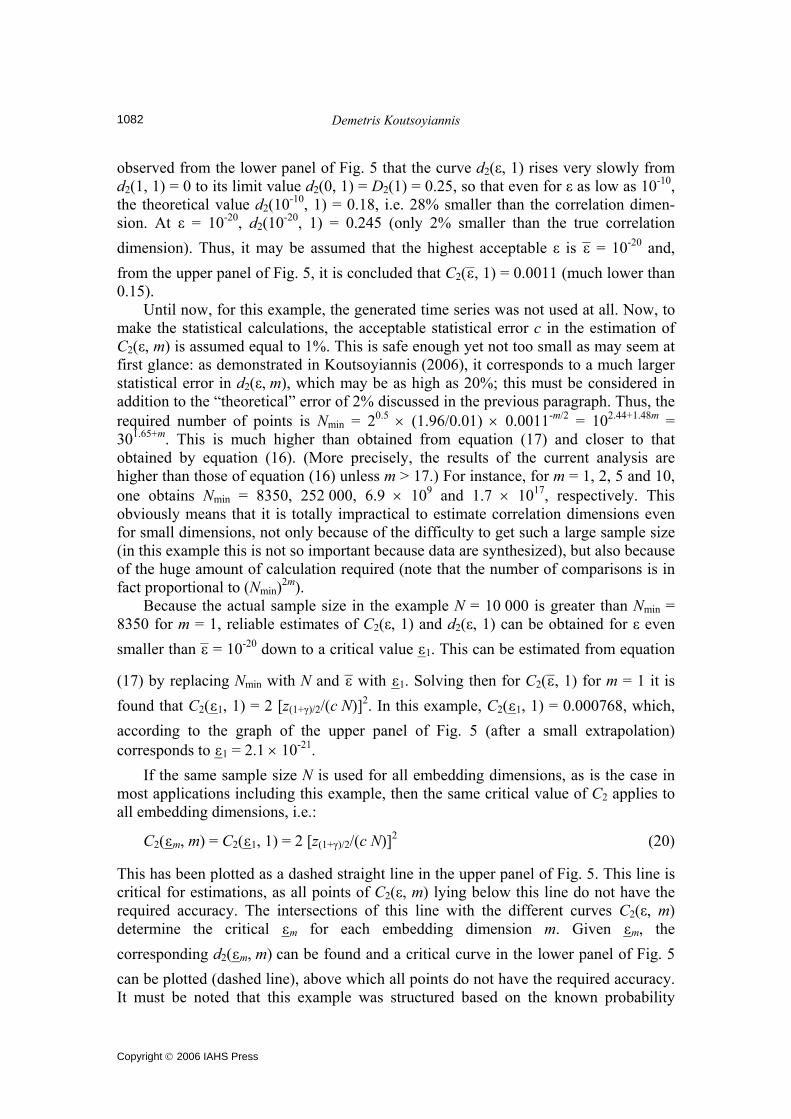
γ = 0.95 for which z(1+γ)/2 = 1.96, an acceptable error c = 3% and a sufficient C2(ε–, 1) = 0.15 (indeed, 20.5(1.96/0.03) 0.15-m/2 = 101.97+0.41m ≈ 102+0.4m). However, equation (19) is more general and the appropriate values of c and C2(ε–, 1) need to be more carefully selected, depending on properties of the time series at hand. This result and its application are demonstrated using an example with a totally random system. Specifically, a sequence of 10 000 random numbers from the Weibull distribution with shape parameter κ = 1/8 (and scale parameter 1) is used. It is known from the discussion above that, although the system is random, the correlation dimension D2(m) does not equal the embedding dimension m, but rather is 2κm = m/4. In addition, since the probability distribution function is known, it is easy to calculate numerically (using equations (11) and (5)) the true (population) values, which the correlation sum C2(ε, 1) and the local slope d2(ε, 1) represent, for any scale ε. Then from equation (18), the true values of C2(ε, m) and d2(ε, m) can be calculated for any embedding dimension m. These have been plotted in Fig. 5 as continuous curves. It is

1E-10

1E-09

1E-08

1E-07

1E-06

1E-05

1E-04

1E-03

1E-02

1E-01

1E+00

1E-20 1E-18 1E-16 1E-14 1E-12 1E-10 1E-08 1E-06 1E-04 1E-02 1E+00ε

C2(ε,

m)

1 2 3 45 6 7 8

Inacurate area

0

0.2

0.4

0.6

0.8

1

1.2

1.4

1.6

1.8

2

1E-20 1E-18 1E-16 1E-14 1E-12 1E-10 1E-08 1E-06 1E-04 1E-02 1E+00ε

d2(ε,

m)

1 2 3 45 6 7 8

Inaccurate area

Fig. 5 Correlation sums C2(ε, m) (upper panel) and their local slopes d2(ε, m) (lower panel) vs scale ε for embedding dimensions m = 1 to 8 calculated from a series of 10 000 independent random points from the Weibull distribution with shape parameter 1/8. Continuous lines represent the true (population) quantities, whose estimates are C2(ε, m) and d2(ε, m).



1082

observed from the lower panel of Fig. 5 that the curve d2(ε, 1) rises very slowly from d2(1, 1) = 0 to its limit value d2(0, 1) = D2(1) = 0.25, so that even for ε as low as 10-10, the theoretical value d2(10-10, 1) = 0.18, i.e. 28% smaller than the correlation dimen-sion. At ε = 10-20, d2(10-20, 1) = 0.245 (only 2% smaller than the true correlation dimension). Thus, it may be assumed that the highest acceptable ε is ε– = 10-20 and, from the upper panel of Fig. 5, it is concluded that C2(ε–, 1) = 0.0011 (much lower than 0.15). Until now, for this example, the generated time series was not used at all. Now, to make the statistical calculations, the acceptable statistical error c in the estimation of C2(ε, m) is assumed equal to 1%. This is safe enough yet not too small as may seem at first glance: as demonstrated in Koutsoyiannis (2006), it corresponds to a much larger statistical error in d2(ε, m), which may be as high as 20%; this must be considered in addition to the “theoretical” error of 2% discussed in the previous paragraph. Thus, the required number of points is Nmin = 20.5 × (1.96/0.01) × 0.0011-m/2 = 102.44+1.48m = 301.65+m. This is much higher than obtained from equation (17) and closer to that obtained by equation (16). (More precisely, the results of the current analysis are higher than those of equation (16) unless m > 17.) For instance, for m = 1, 2, 5 and 10, one obtains Nmin = 8350, 252 000, 6.9 × 109 and 1.7 × 1017, respectively. This obviously means that it is totally impractical to estimate correlation dimensions even for small dimensions, not only because of the difficulty to get such a large sample size (in this example this is not so important because data are synthesized), but also because of the huge amount of calculation required (note that the number of comparisons is in fact proportional to (Nmin)2m). Because the actual sample size in the example N = 10 000 is greater than Nmin = 8350 for m = 1, reliable estimates of C2(ε, 1) and d2(ε, 1) can be obtained for ε even smaller than ε– = 10-20 down to a critical value ε–1. This can be estimated from equation

(17) by replacing Nmin with N and ε– with ε–1. Solving then for C2(ε–, 1) for m = 1 it is found that C2(ε–1, 1) = 2 [z(1+γ)/2/(c N)]2. In this example, C2(ε–1, 1) = 0.000768, which, according to the graph of the upper panel of Fig. 5 (after a small extrapolation) corresponds to ε–1 = 2.1 × 10-21. If the same sample size N is used for all embedding dimensions, as is the case in most applications including this example, then the same critical value of C2 applies to all embedding dimensions, i.e.:

C2(ε–m, m) = C2(ε–1, 1) = 2 [z(1+γ)/2/(c N)]2 (20)

This has been plotted as a dashed straight line in the upper panel of Fig. 5. This line is critical for estimations, as all points of C2(ε, m) lying below this line do not have the required accuracy. The intersections of this line with the different curves C2(ε, m) determine the critical ε–m for each embedding dimension m. Given ε–m, the corresponding d2(ε–m, m) can be found and a critical curve in the lower panel of Fig. 5 can be plotted (dashed line), above which all points do not have the required accuracy. It must be noted that this example was structured based on the known probability



1083

distribution function of the variable. However, the method developed can be applied even when the distribution function is not known, as will be seen in next examples. In conclusion, the proposed approach to determine the required sample size or, equivalently, the adequacy of estimations for a given sample size, involves two characteristic scales: the upper limit ε–, which is common for all embedding dimensions, and the lower limit ε–m which is an increasing function of dimension. The

required sample size Nmin for embedding dimension m is determined setting ε–m = ε–,

whereas for a given N an estimation is accurate when ε–m ≤ ε–. Furthermore, the limits

ε–m and ε– can be determined in a geometrical manner. The steps are the following: 1. Make plots of C2(ε, m) and d2(ε, m) for several embedding dimensions m. 2. In the plot of d2(ε, 1) (i.e. for embedding dimension 1) locate a region where

d2(ε, 1) becomes constant and relatively smooth. Set ε– and ε–1 the upper and lower

limit of this area, respectively (meaning that above ε–, d2(ε, 1) is not constant and below ε–1 it becomes too rough).

3. From the plot of C2(ε, 1) determine C2(ε–1, 1). 4. Set C2(ε–m, m) = C2(ε–1, 1) and determine ε–m for each m.

5. For those m where ε–m ≤ ε– and d2(ε, m) is nearly constant in the interval (ε–m, ε–),

determine D2(m) as the average d2(ε, m) on this interval. For those m where ε–m > ε–, D2(m) cannot be determined.

If for any reason the sample size Nm is different for different embedding dimensions m, the equation in step 4 should be replaced by:

C2(ε–m, m) = C2(ε–1, 1) (N1/Nm)2 (21)

A geometrical view of the procedure is possible by plotting the equations ε = ε– and ε = ε–m in both diagrams of C2(ε, m) and d2(ε, m). In the example of Fig. 5, it is clear

that only D2(1) can be estimated with N = 10 000 points, provided that ε– = 10-20. For instance, a larger ε– = 10-10 would enable estimating D2(2), D2(3) and D2(4) as well, as becomes apparent by observing the dashed curve in the lower panel of Fig. 5. However, the cost to be paid in this case would be the underestimation of dimensions by 28%, as discussed above, which notably is due to theoretical rather than statistical reasons. Effect of autocorrelation Hydrological time series, especially on fine time scales, are characterized by high auto-correlation coefficients. Autocorrelation in stochastic processes may be misleadingly interpreted as low-dimensional determinism when applying the standard algorithms for estimating dimensions. Examples of a highly autocorrelated stochastic processes (including fractional Gaussian noise and other simpler linear and nonlinear processes),



1084

in which the naïve application of the standard methods leads erroneously to low-dimensional attractors (down to 1), have been offered by Osborne & Provenzale (1989); Theiler (1991) and Provenzale et al. (1992) (see also Tsonis, 1992, p. 174). In autocorrelated series, a larger number of data points may not suffice to avoid misleading results. Another important issue is the appropriate selection of the time delay τ in constructing delay vectors. Several authors have discussed this (see, among others, Tsonis, 1992, pp. 151–156; Abarbanel et al., 1993; Kantz & Schreiber, 1997, pp. 130–134; Sivakumar, 2000). The most common approach is to choose as τ the time where the autocorrelation function decays to 1/e, where e is the base of the natural logarithm. Other options are to choose the time where the first minimum of the time-delayed mutual information is located, or to optimize it inside the interval defined by the times of the 1/e decay of autocorrelation and the minimum of mutual information. An additional means of alleviating the effect of temporal correlation is to exclude

1E-08

1E-07

1E-06

1E-05

1E-04

1E-03

1E-02

1E-01

1E+00

1E-06 1E-05 1E-04 1E-03 1E-02 1E-01 1E+00ε

C2(ε,

m)

1 2 3 45 6 7 8

Inaccurate area

Inadequate area

0

0.5

1

1.5

2

2.5

3

3.5

4

1E-06 1E-05 1E-04 1E-03 1E-02 1E-01 1E+00ε

d2(ε,

m)

1 2 3 45 6 7 8

Inaccuratearea

Inadequate area

ε_

ε 1

Fig. 6 Correlation sums C2(ε, m) (upper panel) and their local slopes d2(ε, m) (lower panel) vs scale ε for embedding dimensions m = 1 to 8 calculated from a series of 10 000 autocorrelated random values having approximately Pareto distribution with shape parameter 0.44.



1085

delay vectors that are close in time. This is attained by adopting a relatively high value of w in equation (12) that is used for the estimation of correlation sums. The effect of autocorrelation may act synergistically with the effect of an asymmetric distribution function and the effect of sample size. To demonstrate this, a data series of 10 000 autocorrelated values with J-shaped distribution function was considered. This was generated in the following manner. For the data point yn, eight random numbers were generated at a first step from the Pareto distribution with shape parameter 1/8 and at a second step the random number whose logarithm was nearest to ln yn-1 was chosen as yn. This technique resulted in a series with a Markovian dependence structure with lag-one autocorrelation 0.72 and approximately Pareto distribution with shape parameter κ = 0.44. Therefore it is expected that the correlation dimension in m dimensions of this series will be D2(m) = 2κm = 0.88 m. The empirical estimates of the correlation sums and their local slopes are shown in Fig. 6. These estimates were based on delay time τ = 4, which corresponds to the 1/e (=0.37) decay

1E-08

1E-07

1E-06

1E-05

1E-04

1E-03

1E-02

1E-01

1E+00

1E-06 1E-05 1E-04 1E-03 1E-02 1E-01 1E+00ε

C2(ε,

m)

1 2 3 45 6 7 8

Inaccurate area

Inadequate area

0

1

2

3

4

5

6

7

8

1E-06 1E-05 1E-04 1E-03 1E-02 1E-01 1E+00ε

d2(ε,

m)

1 2 3 45 6 7 8

Inaccuratearea

Inadequate area

ε_ε 1

Fig. 7 Correlation sums C2(ε, m) (upper panel) and their local slopes d2(ε, m) (lower panel) vs scale ε for embedding dimensions m = 1 to 8 calculated from the same series as in Fig. 6, but excluding points having at least one coordinate smaller than 0.01.



1086

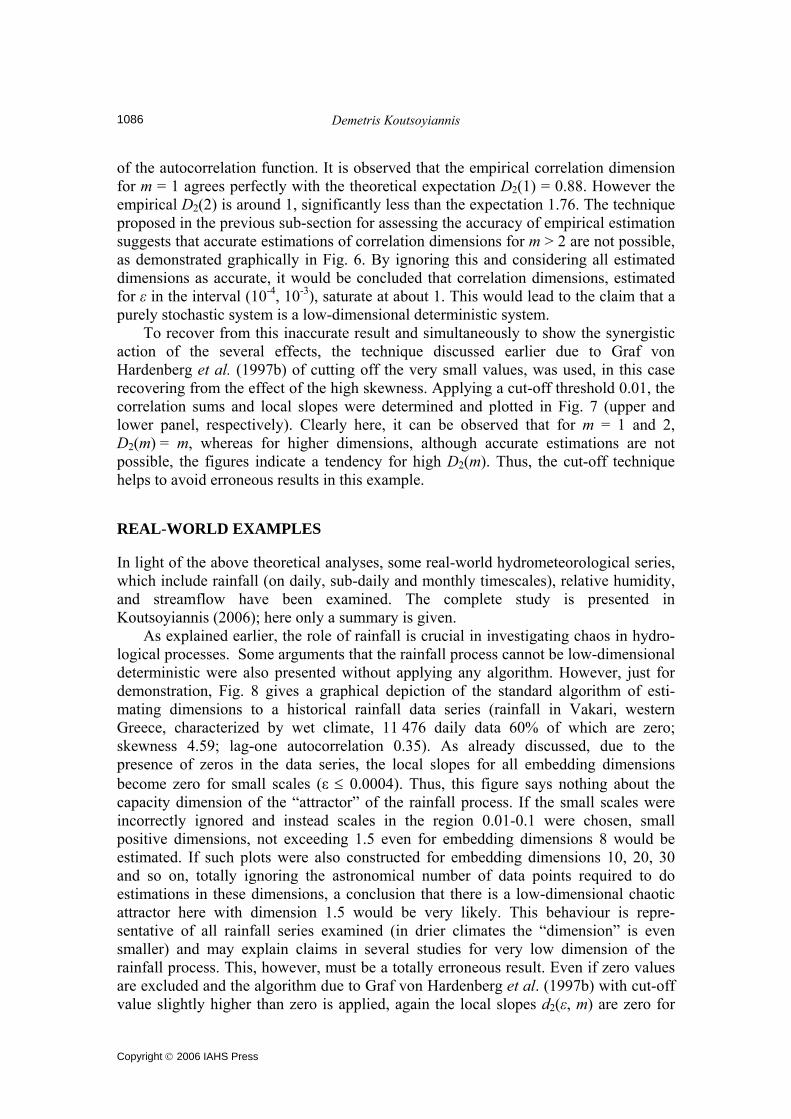
of the autocorrelation function. It is observed that the empirical correlation dimension for m = 1 agrees perfectly with the theoretical expectation D2(1) = 0.88. However the empirical D2(2) is around 1, significantly less than the expectation 1.76. The technique proposed in the previous sub-section for assessing the accuracy of empirical estimation suggests that accurate estimations of correlation dimensions for m > 2 are not possible, as demonstrated graphically in Fig. 6. By ignoring this and considering all estimated dimensions as accurate, it would be concluded that correlation dimensions, estimated for ε in the interval (10-4, 10-3), saturate at about 1. This would lead to the claim that a purely stochastic system is a low-dimensional deterministic system. To recover from this inaccurate result and simultaneously to show the synergistic action of the several effects, the technique discussed earlier due to Graf von Hardenberg et al. (1997b) of cutting off the very small values, was used, in this case recovering from the effect of the high skewness. Applying a cut-off threshold 0.01, the correlation sums and local slopes were determined and plotted in Fig. 7 (upper and lower panel, respectively). Clearly here, it can be observed that for m = 1 and 2, D2(m) = m, whereas for higher dimensions, although accurate estimations are not possible, the figures indicate a tendency for high D2(m). Thus, the cut-off technique helps to avoid erroneous results in this example. REAL-WORLD EXAMPLES In light of the above theoretical analyses, some real-world hydrometeorological series, which include rainfall (on daily, sub-daily and monthly timescales), relative humidity, and streamflow have been examined. The complete study is presented in Koutsoyiannis (2006); here only a summary is given. As explained earlier, the role of rainfall is crucial in investigating chaos in hydro-logical processes. Some arguments that the rainfall process cannot be low-dimensional deterministic were also presented without applying any algorithm. However, just for demonstration, Fig. 8 gives a graphical depiction of the standard algorithm of esti-mating dimensions to a historical rainfall data series (rainfall in Vakari, western Greece, characterized by wet climate, 11 476 daily data 60% of which are zero; skewness 4.59; lag-one autocorrelation 0.35). As already discussed, due to the presence of zeros in the data series, the local slopes for all embedding dimensions become zero for small scales (ε ≤ 0.0004). Thus, this figure says nothing about the capacity dimension of the “attractor” of the rainfall process. If the small scales were incorrectly ignored and instead scales in the region 0.01-0.1 were chosen, small positive dimensions, not exceeding 1.5 even for embedding dimensions 8 would be estimated. If such plots were also constructed for embedding dimensions 10, 20, 30 and so on, totally ignoring the astronomical number of data points required to do estimations in these dimensions, a conclusion that there is a low-dimensional chaotic attractor here with dimension 1.5 would be very likely. This behaviour is repre-sentative of all rainfall series examined (in drier climates the “dimension” is even smaller) and may explain claims in several studies for very low dimension of the rainfall process. This, however, must be a totally erroneous result. Even if zero values are excluded and the algorithm due to Graf von Hardenberg et al. (1997b) with cut-off value slightly higher than zero is applied, again the local slopes d2(ε, m) are zero for



1087

1E-03

1E-02

1E-01

1E+00

1E-06 1E-05 1E-04 1E-03 1E-02 1E-01 1E+00ε

C2(ε,

m)

1 2 3 45 6 7 8

Inadequate area

0

0.5

1

1.5

2

2.5

3

3.5

4

1E-06 1E-05 1E-04 1E-03 1E-02 1E-01 1E+00ε

d2(ε,

m)

1 2 3 45 6 7 8

Inadequate area

ε_

Fig. 8 Correlation sums C2(ε, m) (upper panel) and their local slopes d2(ε, m) (lower panel) vs scale ε for embedding dimensions m = 1 to 8 calculated from the daily rainfall series at the Vakari raingauge.

small scales. This is the result of round-off errors in the data values, rather than a theoretically consistent result. But in this case the local slopes tend to more reasonable values (in this example to about 0.7 and 1.4 for m = 1 and 2, respectively; Koutsoyiannis, 2006). To minimize the effect of round-off errors, the cut-off value should be increased to 2 mm. In this case the sample size becomes too low to allow for any accurate estimation but shows (Koutsoyiannis, 2006) that the correlation dimension D2(m) tends to the embedding dimension m, which means that the time series is better represented as the outcome of a stochastic process. If the presence of zeros in a rainfall time series is a strong obstacle to analysing the presence of chaos, one may think that going to a much finer timescale and limiting the analysis strictly to a rainy period (a single storm) one could find the deterministic chaos. The idea of a deterministic (meaning low-dimensional?) evolution of a storm has been favoured long before hydrologists became involved with chaos. For example, Eagleson (1970, p. 184) states “The spacing and sizing of individual events in the sequence is probabilistic, while the internal structure of a given storm may be largely deterministic”.



1088

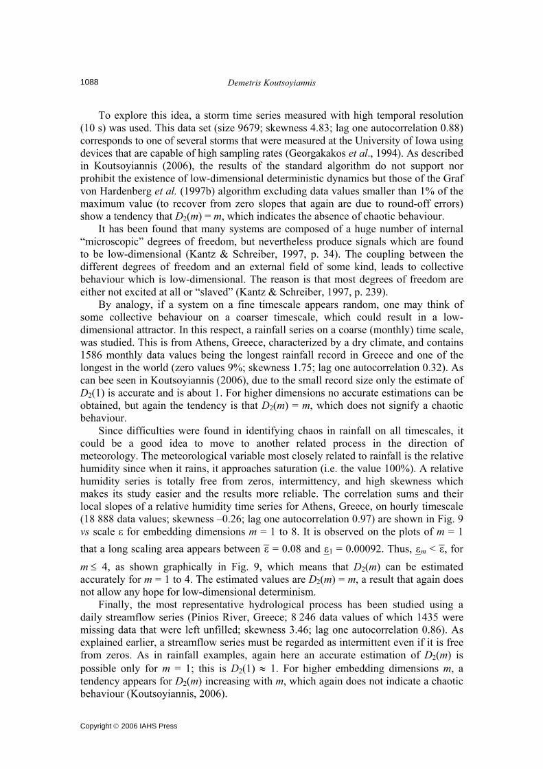
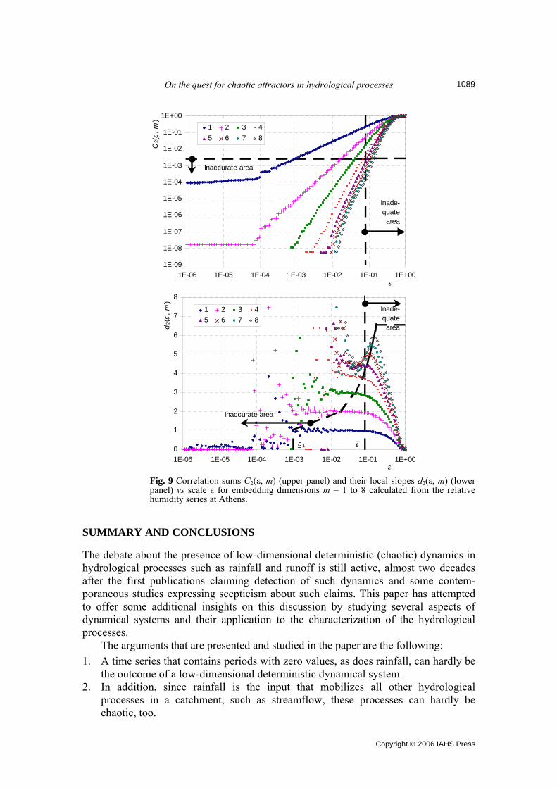
To explore this idea, a storm time series measured with high temporal resolution (10 s) was used. This data set (size 9679; skewness 4.83; lag one autocorrelation 0.88) corresponds to one of several storms that were measured at the University of Iowa using devices that are capable of high sampling rates (Georgakakos et al., 1994). As described in Koutsoyiannis (2006), the results of the standard algorithm do not support nor prohibit the existence of low-dimensional deterministic dynamics but those of the Graf von Hardenberg et al. (1997b) algorithm excluding data values smaller than 1% of the maximum value (to recover from zero slopes that again are due to round-off errors) show a tendency that D2(m) = m, which indicates the absence of chaotic behaviour. It has been found that many systems are composed of a huge number of internal “microscopic” degrees of freedom, but nevertheless produce signals which are found to be low-dimensional (Kantz & Schreiber, 1997, p. 34). The coupling between the different degrees of freedom and an external field of some kind, leads to collective behaviour which is low-dimensional. The reason is that most degrees of freedom are either not excited at all or “slaved” (Kantz & Schreiber, 1997, p. 239). By analogy, if a system on a fine timescale appears random, one may think of some collective behaviour on a coarser timescale, which could result in a low-dimensional attractor. In this respect, a rainfall series on a coarse (monthly) time scale, was studied. This is from Athens, Greece, characterized by a dry climate, and contains 1586 monthly data values being the longest rainfall record in Greece and one of the longest in the world (zero values 9%; skewness 1.75; lag one autocorrelation 0.32). As can bee seen in Koutsoyiannis (2006), due to the small record size only the estimate of D2(1) is accurate and is about 1. For higher dimensions no accurate estimations can be obtained, but again the tendency is that D2(m) = m, which does not signify a chaotic behaviour. Since difficulties were found in identifying chaos in rainfall on all timescales, it could be a good idea to move to another related process in the direction of meteorology. The meteorological variable most closely related to rainfall is the relative humidity since when it rains, it approaches saturation (i.e. the value 100%). A relative humidity series is totally free from zeros, intermittency, and high skewness which makes its study easier and the results more reliable. The correlation sums and their local slopes of a relative humidity time series for Athens, Greece, on hourly timescale (18 888 data values; skewness –0.26; lag one autocorrelation 0.97) are shown in Fig. 9 vs scale ε for embedding dimensions m = 1 to 8. It is observed on the plots of m = 1 that a long scaling area appears between ε– = 0.08 and ε–1 = 0.00092. Thus, ε–m < ε–, for m ≤ 4, as shown graphically in Fig. 9, which means that D2(m) can be estimated accurately for m = 1 to 4. The estimated values are D2(m) = m, a result that again does not allow any hope for low-dimensional determinism. Finally, the most representative hydrological process has been studied using a daily streamflow series (Pinios River, Greece; 8 246 data values of which 1435 were missing data that were left unfilled; skewness 3.46; lag one autocorrelation 0.86). As explained earlier, a streamflow series must be regarded as intermittent even if it is free from zeros. As in rainfall examples, again here an accurate estimation of D2(m) is possible only for m = 1; this is D2(1) ≈ 1. For higher embedding dimensions m, a tendency appears for D2(m) increasing with m, which again does not indicate a chaotic behaviour (Koutsoyiannis, 2006).



1089

1E-09

1E-08

1E-07

1E-06

1E-05

1E-04

1E-03

1E-02

1E-01

1E+00

1E-06 1E-05 1E-04 1E-03 1E-02 1E-01 1E+00ε

C2(ε,

m)

1 2 3 45 6 7 8

Inaccurate area

Inade-quate area

0

1

2

3

4

5

6

7

8

1E-06 1E-05 1E-04 1E-03 1E-02 1E-01 1E+00ε

d2(ε,

m)

1 2 3 45 6 7 8

Inaccurate area

Inade-quate area

ε_

ε 1

Fig. 9 Correlation sums C2(ε, m) (upper panel) and their local slopes d2(ε, m) (lower panel) vs scale ε for embedding dimensions m = 1 to 8 calculated from the relative humidity series at Athens.

SUMMARY AND CONCLUSIONS The debate about the presence of low-dimensional deterministic (chaotic) dynamics in hydrological processes such as rainfall and runoff is still active, almost two decades after the first publications claiming detection of such dynamics and some contem-poraneous studies expressing scepticism about such claims. This paper has attempted to offer some additional insights on this discussion by studying several aspects of dynamical systems and their application to the characterization of the hydrological processes. The arguments that are presented and studied in the paper are the following: 1. A time series that contains periods with zero values, as does rainfall, can hardly be

the outcome of a low-dimensional deterministic dynamical system. 2. In addition, since rainfall is the input that mobilizes all other hydrological

processes in a catchment, such as streamflow, these processes can hardly be chaotic, too.



1090

3. An attractor dimension as low as 1 or even smaller, which in some cases were claimed for hydrological processes, would be directly visualized via delay represen-tation graphs. This however, has never come into light, simply because in fact such graphs manifest space filling clouds rather than one-dimensional structures.

4. The attractor dimension must be consistent with the dimension used to embed it according to Whitney’s embedding theorem. For example, if an attractor dimension were 1 or less, then a 3D embedding space would suffice to embed it. The fact that the required embedding dimension in some cases was reported to be as high as 10-40 simply indicates inconsistency of results.

5. The embedding theorems are in fact based on the concept of the capacity dimension whereas the standard algorithms to determine attractor dimensions use the concept of the correlation dimension. The two dimensions are most often identical but it is proved that if the distribution function is J-shaped with high skewness, as is the case with hydrological processes on fine timescales, the correlation dimension is smaller than the capacity dimension. This may produce misleadingly small estimated dimensions.

6. Intermittency (which is apparent in hydrological processes—not only in rainfall but in streamflow as well) is another factor that can result in a misleading low attractor dimension even in infinite-dimensional systems. This known result has not been given the required attention in hydrological studies investigating chaos.

7. Another known issue is the fact that very many data points are needed to recover chaos from time series, which are hardly available in hydrological processes. This has not been given the required attention in hydrological studies (albeit mentioned sometimes) because perhaps the calculation of the sample size is ambiguous. Here, using statistical reasoning, a rigorous methodology has been proposed for estimating the required sample size for a certain embedding dimension or, conversely, the maximum allowed embedding dimension for a given sample size. It turns out that the required sample size in hydrological time series may be even more exceptionally high than believed due to the asymmetric distribution functions.

8. The high autocorrelation that characterizes many hydrological processes, mostly on fine timescales, is another factor that, acting synergistically with the other factors described above, may be misleadingly interpreted as low-dimensional determinism.

All these arguments have been demonstrated using appropriately synthesized theoretical examples. Finally, in light of the theoretical analyses and arguments, typical real-world hydrometeorological time series, which include rainfall (on daily, fine sub-daily, and monthly timescales), relative humidity, and streamflow, have been explored and none of them is found to indicate the presence of chaos but, rather, correspond to the outcomes of stochastic systems. Acknowledgments I am grateful to the editor Zbigniew Kundzewicz and the reviewers Daniele Veneziano and Timothy Cohn for their positive and encouraging critiques, suggestions, comments, and detailed checks and corrections to the text and the mathematics. My thanks to DV extend to his equally positive review on an earlier version of the paper submitted to another journal (2001) and rejected.



1091

REFERENCES Abarbanel, H. D. I., Brown, R., Sidorowich, J. J. & Tsimring, L. S. (1993) The analysis of observed chaotic data in

physical systems, Rev. Mod. Phys., 65(4), 1331–1391. Eagleson, P. S. (1970) Dynamic Hydrology, McGraw–Hill, New York, USA. Georgakakos, K. P., Carsteanu, A. A., Sturdevant, P. L. & Cramer, J. A. (1994) Observation and analysis of Midwestern

rain rates. J. Appl. Met. 33, 1433–1444. Gershenfeld, N. A. & Weigend, A. S. (1993) The future of time series: learning and understanding. In: Time Series

Prediction: Forecasting the Future and Understanding the Past (ed. by A. S. Weigend & N. A. Gershenfeld), 1–70, SFI Stud. in the Sci. of Complex., Proc. vol. XV, Addison-Wesley, Reading, Massachusetts, USA.

Graf von Hardenberg, J., Paparella, F., Platt, N., Provenzale, A. & Spiegel, E. A. (1997a) Through a glass darkly. In: Nonlinear Signal and Image Analysis (ed. by J. R. Buchler & H. Kandrup), 79–98. Annals of the New York Academy of Sciences no. 808.

Graf von Hardenberg, J., Paparella, F., Platt, N., Provenzale, A., Spiegel, E. A. & Tesser, C. (1997b) Missing motor of on–off intermittency. Physical Review E 55(1), 58–64.

Grassberger, P. (1983) Generalized dimensions of strange attractors. Phys. Lett. 97A(6), 227–230. Grassberger, P. & Procaccia, I. (1983) Characterization of strange attractors. Phys. Rev. Lett. 50(5), 346–349. Grassberger, P., Schreiber, T. & Schaffrath, C. (1991) Nonlinear time sequence analysis. Int. J. Bifurcation and Chaos 1,

521. Hübner, U., Weiss, C. O., Abraham, N. & Tang, D. (1993) Lorenz-like chaos in NH3-FIR lasers. In: Time Series

Prediction: Forecasting the Future and Understanding the Past (ed. by A. S. Weigend & N. A. Gershenfeld), 73–105. SFI Studies in the Sciences of Complexity, Proc. vol. XV. Addison-Wesley, Reading, Massachusetts, USA.

Kantz, H. & Schreiber, T. (1997) Nonlinear Time Series Analysis, Cambridge University Press, Cambridge, UK. Koutsoyiannis, D. (2006) On the quest for chaotic attractors in hydrological processes: additional information. Internal

Report, Dept of Water Resources, National Technical University of Athens (http://www.itia.ntua.gr/e/docinfo/714/). Koutsoyiannis, D., Yao, H. & Georgakakos, A. (2006) Multiyear behaviour and monthly simulation and forecasting of the

Nile River flow. In: 2006 General Assembly of the European Geosciences Union, Vienna. Geophys. Res. Abstracts 8, 05046, European Geosciences Union.

Lasota, A. & Mackey, M. C. (1994) Chaos, Fractals, and Noise, Springer-Verlag, New York, USA. Nerenberg, M. A. H. & Essex, C. (1990) Correlation dimension and systematic geometric effects. Phys. Rev. A, 42, 7065–

7074. Osborne, A. R. & Provenzale, A. (1989) Finite correlation dimension for stochastic systems with power-law spectra.

Physica D 35, 357–381. Provenzale, A., Smith, L. A., Vio, R. & Murante, G. (1992) Distinguishing between low-dimensional dynamics and

randomness in measured time series. Physica D 58, 31–49. Rényi, A. (1970) Probability Theory. North-Holland, Amsterdam, The Netherlands. Rössler, O. E. (1979) An equation for hyperchaos. Phys. Lett. A 71, 155. Sauer, T., Yorke, J. & Casdagli, M. (1991) Embedology. J. Statist. Phys. 65(3/4), 579–616. Schertzer, D., Tchguirinskaia, I., Lovejoy, S., Hubert, P., Bendjoudi, H. & Larchvêque, M. (2002) Which chaos in the

rainfall–runoff process? Hydrol. Sci. J. 47(1), 139–148. Sivakumar, B., Berndtsson, R., Olsson, J. & Jinno, K. (2001) Evidence of chaos in the rainfall–runoff process. Hydrol. Sci.

J. 46(1), 131–146. Sivakumar, B., Berndtsson, R., Olsson, J. & Jinno, K. (2002) Reply to “Which chaos in the rainfall–runoff process?”

Hydrol. Sci. J. 47(1), 149–158. Sivakumar, B. (2000) Chaos theory in hydrology: important issues and interpretations. J. Hydrol. 227, 1–20. Sivakumar, B. (2004) Chaos theory in geophysics: past, present and future. Chaos, Solitons and Fractals 19, 441–462. Smith, L. A. (1988) Intrinsic limits on dimension calculations. Phys. Lett. A 133, 283–288. Takens, F. (1981) Detecting strange attractors in turbulence. In: Dynamical Systems and Turbulence (ed. by D. A. Rand &

L.-S. Young), 336–381. Lecture Notes in Mathematics no. 898. Springer-Verlag, New York, USA. Theiler, J. (1991) Some comments on the correlation dimension of 1/fa noise. Phys. Lett. A 155, 480–492. Tsallis, C. (2004) Nonextensive statistical mechanics: construction and physical interpretation. In: Nonextensive Entropy,

Interdisciplinary Applications (ed. by M. Gell-Mann & C. Tsallis). Oxford University Press, New York, USA. Tsonis, A. A. (1992) Chaos: From Theory to Applications. Plenum, New York, USA. Tsonis, A. A., Elsner, J. B. & Georgakakos, K. (1993) Estimating the dimension of weather and climate attractors:

Important issues on the procedure and interpretation. J. Atmos. Sci. 50(15), 2249–2555. Wang, Q. & Gan, T. Y. (1998) Biases of correlation dimension estimates of streamflow data in the Canadian prairies.

Water Resour. Res. 34(9), 2329–2339. Whitney, H. (1936) Differentiable manifolds. Ann. Math. 37, 645. Received 12 January 2006; accepted 19 June 2006

Documents

On the quest for chaotic attractors in hydrological processes · On the quest for chaotic attractors in hydrological processes ... in some cases, merely the careful application of