Embed Size (px)
Citation preview
Extremes (2007) 10:235–248DOI 10.1007/s10687-007-0043-1
On limit laws for sums of Pfeifer records
Jose A. Villasenor · Barry C. Arnold
Received: 7 November 2006 / Revised: 27 July 2007 /Accepted: 15 August 2007 / Published online: 24 October 2007© Springer Science + Business Media, LLC 2007
Abstract The problem of determining limiting distributions for sums ofrecords has been studied by several authors who have considered a variety ofassumptions sufficient to ensure that sums of records properly normalized willconverge to a non-degenerate distribution. As a parallel to these endeavors,it is of interest to establish conditions under which the sum of Pfeifer records,properly normalized, converges. Pfeifer records are defined under the assump-
tion that initial observations are i.i.d. with common survival function(
F0
)α0
and following the (n-1)-th record value the observations are assumed to have
survival function(
F0
)αn
, n = 1, 2, .... The study of the asymptotic behavior ofsums of Pfeifer records constitutes a natural generalization of work on sumsof classical records. The present paper introduces conditions under which thelimit distribution of sums of Pfeifer records is non-degenerate.
Keywords Sums of dependent random variables · Record values ·Asymptotic distributions · Limit laws · Regularly varying functions ·Generalized order statistics
AMS 2000 Subject Classification 60E05 · 60F99
J. A. Villasenor (B)Colegio de Postgraduados, Montecillo, Mexicoe-mail: [email protected]
B. C. ArnoldUniversity of California, Riverside, CA, USA
236 J.A. Villasenor, B.C. Arnold
1 Introduction
Consider X1, X2, . . . , a sequence of independent identically distributed ran-dom variables with common continuous distribution function F and, in ab-solutely continuous cases, density f . An observation in this sequence is arecord (strictly speaking an upper record) if it exceeds in value all the ob-servations preceding it in the sequence. Lower records can be analogouslydefined. A convenient reference for discussion of the basic and asymptoticdistribution theory of record values is Arnold et al. (1998). By conventionthe first observation X1 is considered to be a record, the zero’th record. Thesequence of record values will be denoted by X(0), X(1), X(2), . . . Arnold andVillaseñor (1998) initiated discussion of the asymptotic distribution of sumsof records. They were able to identify appropriate limiting distributions inonly a few special cases. Subsequently considerable progress has been madeon resolving this problem. In this paper, the focus will be on the problemof determining the asymptotic distribution of sums of Pfeifer records whichwill subsume and extend results on sums of classical records. We begin byrecalling relevant theory for sums of classical records in Section 2. The Pfeifergeneralization will be discussed in subsequent Sections.
2 Records and Sums of Records
As described in the introduction the sequence of observations will be denotedby X1, X2, . . ., with common continuous distribution function F. The corre-sponding sequence of records will be denoted by X(0), X(1), X(2), . . . . For eachn = 0, 1, 2, ...we denote the sum of the first n records by
Tn =n∑
i=0
X(i).
We will use an asterisk notation to denote the special case of standard expo-nential variables, their corresponding records and sums of records. Thus wehave X∗
i denoting the i’th exponential observation, X∗(i), the i’th exponential
record and T∗n, the sum of the first n exponential records. The lack of memory
property of the exponential distribution guarantees that the correspondingrecord increments (differences between successive records) will also be expo-nentially distributed and will be independent. Consequently the distribution ofexponential records is particularly simple to derive. We have
X∗(i)
d=i∑
j=0
X∗j ∼ �(i + 1, 1).
To study record values corresponding to the distribution FX(x) we use the factthat, if we define
ψX(u) = F−1X
(1 − e−u)
where
F−1X (y) = sup{x : FX(x) ≤ y},
On limit laws for sums of Pfeifer records 237
then
Xid= ψX(X∗
i )
and
X(i)d= ψX
(X∗
(i)
)
This representation is also valid for the joint distribution of records. Thusfor any n we have
(X(0), X(1), . . . , X(n)
) d=(
ψX(X∗0 ), ψX(X∗
0 + X∗1 ), . . . , ψX
(n∑
i=0
X∗i
)). (1)
where X∗0 , X∗
1 , ...... is a sequence of i.i.d. exp(1) random variables.Resnick (1973) identified all possible limit laws for records. They are nor-
mal, lognormal and negative lognormal. Which limit law applies depends onthe tail behavior of the function ψ . We are interested instead in the asymptoticdistribution of the sum of records Tn = ∑n
i=0 X(i). Such a random variable canbe written as a function of i.i.d. standard exponential variables, thus:
Tn =n∑
i=0
ψX
⎛⎝
i∑j=0
X∗j
⎞⎠ . (2)
Observe that the function ψ appearing in Eq. 2 can be any continuousmapping from (0, ∞) into �. Since the X∗
j ’s are positive random variables,it is evident that the asymptotic behavior of Tn, just as was the asymptoticbehavior of X(n), will be governed by the upper tail behavior of ψ. Although itwill take us outside of the realm of records, it is also intriguing to speculate howcrucial it is that the random variables appearing in Eq. 2 have an exponentialdistribution. Thus we may wish to consider the more general problem ofidentifying the asymptotic distribution of random variables of the form
Un =n∑
i=0
ψ
⎛⎝
i∑j=0
X j
⎞⎠ (3)
where ψ : (0, ∞) −→ � is continuous and the X j’s are i.i.d. positive randomvariables with common distribution function G. For some functions ψ thisproblem has been studied by Rempala and Wesolowski (2002) and Bose et al.(2003). For a detailed review and results related to the asymptotic distributionof model (3) see Arnold and Villaseñor (2006).
3 Sums of Pfeifer Records
In the Pfeifer record model (Pfeifer 1984), it is assumed that initial observa-
tions are i.i.d. with common survival function(
F0
)α0
. Following the n − 1’th
238 J.A. Villasenor, B.C. Arnold
record value the observations are assumed to have survival function(
F0
)αn
,
n = 1, 2, .... It is convenient to introduce the notation
ψ0(u) = F−10 (1 − e−u).
If we denote the corresponding record sequence by {Rn}∞n=0 and the corre-sponding sums of records by
Sn =n∑
j=0
R j
it is not difficult to verify that
Snd=
n∑i=0
ψ0
⎛⎝
i∑j=0
β jX∗j
⎞⎠
where the X∗j ’s are i.i.d. standard exponential variables and where we have
defined β j = α−1j .
Our goal is to study the asymptotic behavior of Sn. Note that, if β j = β0 forevery j, then this reduces to sums of classical records.
In the special case in which ψ0(u) = u, our observations are exponential, andwe have
Snd=
n∑i=0
⎛⎝
i∑j=0
β jX∗j
⎞⎠ =
n∑j=0
(n + 1 − j )β jX∗j
It follows that
E(Sn) =n∑
j=0
(n + 1 − j )β j
and
Var(Sn) =n∑
j=0
(n + 1 − j )2β2j .
As in the standard record case, we can use the Liapounov condition to identifyconfigurations which will lead to an asymptotic normal distribution for Sn.Thus, a sufficient condition to ensure that
(Sn − E(Sn))/√
Var(Sn)d→ Z � N(0, 1)
is that
limn→∞
⎛⎝
n∑j=0
(n + 1 − j )3β3j
⎞⎠/⎛
⎝n∑
j=0
(n + 1 − j )2β2j
⎞⎠
3/2
= 0.

On limit laws for sums of Pfeifer records 239
For example, if the sequence of β j’s is bounded above and below, i.e., if0 < γ ≤ β j ≤ δ < ∞ for every j, then we have
0 < limn→∞
⎛⎝
n∑j=0
(n + 1 − j )3β3j
⎞⎠/⎛
⎝n∑
j=0
(n + 1 − j )2β2j
⎞⎠
3/2
≤ (δ/γ )3 limn→∞
⎛⎝
n∑j=0
(n + 1 − j )3
⎞⎠/⎛
⎝n∑
j=0
(n + 1 − j )2
⎞⎠
3/2
= (δ/γ )3 limn→∞
((n + 1)2(n + 2)2
4
)/((n + 1)(n + 2)(2n + 3)
6
)3/2
= 0.
Thus, in this case (the exponential case in which ψ0(u) = u) asymptoticnormality of the sums of Pfeifer records is assured. In the next Section, weconsider more general choices for the function ψ0.
4 Sums of Pfeifer Records and Regularly Varying Functions
Consideration of sums of Pfeifer records for non-exponential variables leads usto study the more general problem of identifying the asymptotic distributionfor random variables of the form
Wn =n∑
i=0
ψ
⎛⎝
i∑j=0
β jX j
⎞⎠ (4)
where the X j’s are i.i.d. non-negative random variables and the β j’s are positiveconstants while ψ : �+ → � is continuous. The sums of Pfeifer records modelis included in Eq. 4. It corresponds to the case in which the X j’s are i.i.d.standard exponential random variables. A result for random variables of theform Eq. 4 under the condition that the function ψ is regularly varying at ∞ iscontained in the next theorem.
Theorem 4.1 Let{
X j}∞
j=0 be a sequence of i.i.d. r.v.’s with distribution Fwhich is absolutely continuous, has support [0, ∞) with F (0+) = 0 and finitemoment generating function. Suppose ψ is a non-decreasing function that isregularly varying at ∞ of order α ≥ 1, which is twice differentiable with ψ ′′monotone and h is a positive non-decreasing function which is regularly varyingat ∞ of order δ ≥ 0, then for μ and σ 2, the mean and variance of F, as n → ∞
1
cnσ
⎧⎨⎩Wn −
n∑k=0
ψ
⎛⎝μ
k∑j=0
β j
⎞⎠⎫⎬⎭
d→ Z � N(0, 1),
240 J.A. Villasenor, B.C. Arnold
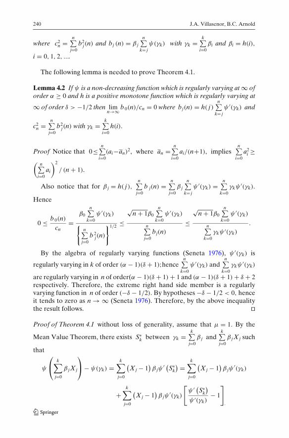
where c2n =
n∑j=0
b2j(n) and bj (n) = β j
n∑k= j
ψ(γk) with γk =k∑
i=0βi and βi = h(i),
i = 0, 1, 2, ....
The following lemma is needed to prove Theorem 4.1.
Lemma 4.2 If ψ is a non-decreasing function which is regularly varying at ∞ oforder α ≥ 0 and h is a positive monotone function which is regularly varying at
∞ of order δ > −1/2 then limn→∞ b 0(n)/cn = 0 where bj(n) = h( j )
n∑k= j
ψ ′(γk) and
c2n =
n∑j=0
b2j(n) with γk =
k∑i=0
h(i).
Proof Notice that 0≤n∑
i=0(ai−an)
2, where an =n∑
i=0ai/(n+1), implies
n∑i=0
a2i ≥
(n∑
i=0ai
)2
/ (n + 1).
Also notice that for β j = h( j ),n∑
j=0b j(n) =
n∑j=0
β j
n∑k= j
ψ ′(γk) =n∑
k=0γkψ
′(γk).
Hence
0 ≤ b 0(n)
cn=
β0
n∑k=0
ψ ′(γk)
{n∑
j=0b 2
j(n)
}1/2 ≤√
n + 1β0
n∑k=0
ψ ′(γk)
n∑j=0
bj(n)
≤√
n + 1β0
n∑k=0
ψ ′(γk)
n∑k=0
γkψ ′(γk)
.
By the algebra of regularly varying functions (Seneta 1976), ψ ′(γk) is
regularly varying in k of order (α − 1)(δ + 1);hencen∑
k=0ψ ′(γk) and
n∑k=0
γkψ′(γk)
are regularly varying in n of order(α − 1)(δ + 1) + 1 and (α − 1)(δ + 1) + δ + 2respectively. Therefore, the extreme right hand side member is a regularlyvarying function in n of order (−δ − 1/2). By hypotheses −δ − 1/2 < 0, henceit tends to zero as n → ∞ (Seneta 1976). Therefore, by the above inequalitythe result follows. ��
Proof of Theorem 4.1 without loss of generality, assume that μ = 1. By the
Mean Value Theorem, there exists S∗k between γk =
k∑j=0
β j andk∑
j=0β jX j such
that
ψ
⎛⎝
k∑j=0
β jX j
⎞⎠ − ψ(γk) =
k∑j=0
(X j − 1
)β jψ
′ (S∗k
) =k∑
j=0
(X j − 1
)β jψ
′(γk)
+k∑
j=0
(X j − 1
)β jψ
′(γk)
[ψ ′ (S∗
k
)
ψ ′(γk)− 1
]
·
On limit laws for sums of Pfeifer records 241
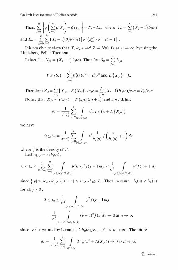
Then,n∑
k=0
{ψ
(k∑
j=0β jX j
)−ψ(γk)
}=Tn+En, where Tn =
n∑j=0
(X j − 1
)bj(n)
and En =n∑
k=0
k∑j=0
(X j − 1
)β jψ
′(γk)[ψ ′ (S∗
k
)/ψ ′(γk) − 1
].
It is possible to show that Tn/cnσ →d Z ∼ N(0, 1) as n → ∞ by using theLindeberg–Feller Theorem.
In fact, let X jn = (X j − 1
)bj(n). Then for Sn =
n∑j=0
X jn,
Var (Sn) =n∑
j=0
b2j(n)σ 2 = c2
nσ2 and E
{X jn
} = 0.
Therefore Zn =n∑
j=0
{X jn−E
(X jn
)}/cnσ =
n∑j=0
(X j−1
)b j(n)/cnσ =Tn/cnσ
Notice that X jn ∼ F jn(x) = F(x/bj(n) + 1
)and if we define
δn = 1
σ 2c2n
n∑j=0
∫
|x|≥εcnσ
x2dF jn(x + E
{X jn
})
we have
0 ≤ δn = 1
σ 2c2n
n∑j=0
∫
|x|≥εcnσ
x2 1
bj(n)f(
xbj(n)
+ 1
)dx
where f is the density of F.Letting y = x/bj(n) ,
0 ≤ δn ≤ 1
σ 2c2n
n∑j=0
∫
|y|≥εcnσ/b j(n)
b2j(n)y2 f (y + 1)dy ≤ 1
σ 2
∫
|y|≥εcnσ/b 0(n)
y2 f (y + 1)dy
since{|y| ≥ εcnσ/bj(n)
} ⊆ {|y| ≥ εcnσ/b 0(n)} . Then. because bj(n) ≤ b 0(n)
for all j ≥ 0 ,
0 ≤ δn ≤ 1
σ 2
∫
|y|≥εcnσ/b 0(n)
y2 f (y + 1)dy
= 1
σ 2
∫
|v−1|≥εcnσ/b 0(n)
(v − 1)2 f (v)dv → 0 as n → ∞
since σ 2 < ∞ and by Lemma 4.2 b 0(n)/cn → 0 as n → ∞ . Therefore,
δn = 1
σ 2c2n
n∑j=0
∫
|x|≥εcn
dF jn(x2 + E(X jn)) → 0 as n → ∞
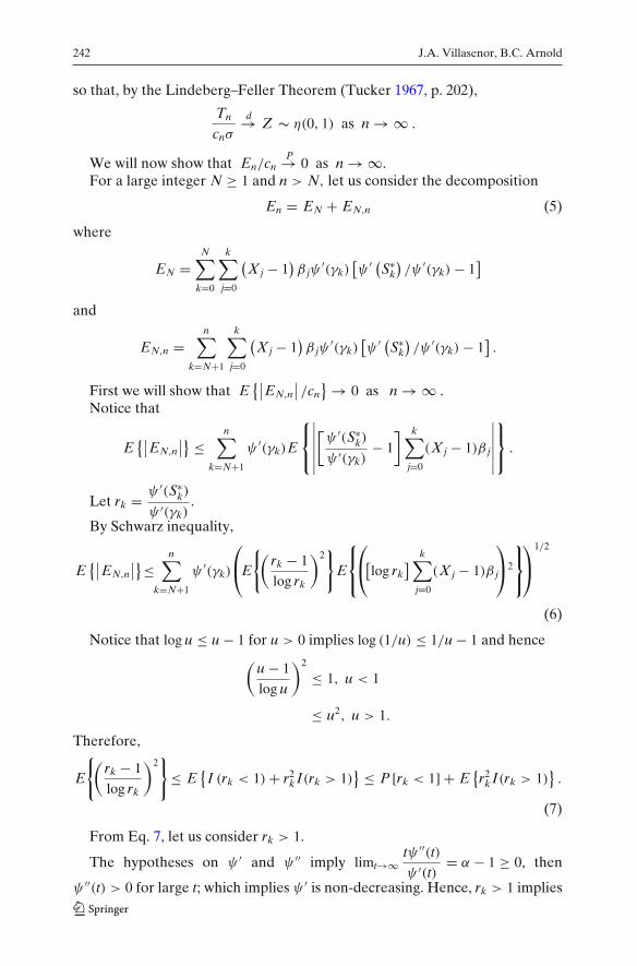
242 J.A. Villasenor, B.C. Arnold
so that, by the Lindeberg–Feller Theorem (Tucker 1967, p. 202),
Tn
cnσ
d→ Z ∼ η(0, 1) as n → ∞ .
We will now show that En/cnP→ 0 as n → ∞.
For a large integer N ≥ 1 and n > N, let us consider the decomposition
En = EN + EN,n (5)
where
EN =N∑
k=0
k∑j=0
(X j − 1
)β jψ
′(γk)[ψ ′ (S∗
k
)/ψ ′(γk) − 1
]
and
EN,n =n∑
k=N+1
k∑j=0
(X j − 1
)β jψ
′(γk)[ψ ′ (S∗
k
)/ψ ′(γk) − 1
].
First we will show that E{∣∣EN,n
∣∣ /cn} → 0 as n → ∞ .
Notice that
E{∣∣EN,n
∣∣} ≤n∑
k=N+1
ψ ′(γk)E
⎧⎨⎩
∣∣∣∣∣∣
[ψ ′(S∗
k)
ψ ′(γk)− 1
] k∑j=0
(X j − 1)β j
∣∣∣∣∣∣
⎫⎬⎭ .
Let rk = ψ ′(S∗k)
ψ ′(γk).
By Schwarz inequality,
E{∣∣EN,n
∣∣}≤n∑
k=N+1
ψ ′(γk)
⎛⎝E
{(rk − 1
log rk
)2}
E
⎧⎨⎩
⎛⎝[log rk
] k∑j=0
(X j − 1)β j
⎞⎠2
⎫⎬⎭
⎞⎠
1/2
(6)
Notice that log u ≤ u − 1 for u > 0 implies log (1/u) ≤ 1/u − 1 and hence(
u − 1
log u
)2
≤ 1, u < 1
≤ u2, u > 1.
Therefore,
E
{(rk − 1
log rk
)2}
≤ E{
I (rk < 1) + r2k I(rk > 1)
} ≤ P [rk < 1] + E{r2
k I(rk > 1)}.
(7)
From Eq. 7, let us consider rk > 1.
The hypotheses on ψ ′ and ψ ′′ imply limt→∞tψ ′′(t)ψ ′(t)
= α − 1 ≥ 0, then
ψ ′′(t) > 0 for large t; which implies ψ ′ is non-decreasing. Hence, rk > 1 implies
On limit laws for sums of Pfeifer records 243
S∗k ≥ γk. Therefore, since γk → ∞ as k → ∞, for some constant C = α − 1 +
ε > 0 for a given ε > 0 and k sufficiently large,
r2k = exp
{2∫ S∗
k
γk
tψ ′′(t)ψ ′(t)
dtt
}≤ exp
{2C
∣∣∣∣∣∫ S∗
k
γk
dtt
∣∣∣∣∣
}. (8)
Using again log u ≤ u − 1, for u > 0, and the fact that S∗k is in between γk
andk∑
j=0X jβ j,
r2k ≤ exp
{2Cγk
∣∣S∗k − γk
∣∣}
≤ exp
⎧⎨⎩
2Cγk
∣∣∣∣∣∣k∑
j=0
(X j − 1
)β j
∣∣∣∣∣∣
⎫⎬⎭
≤ exp
⎧⎨⎩
2Cγk
k∑j=0
X jβ j + 2C
⎫⎬⎭ ≤ C1
k∏j=0
exp
{2CX jβ j
γk
}, (9)
for some real constant C1 > 0.
By hypotheses, there exists the moment generating function of F denoted
by m(t) for t ∈ (−t0, t0) , for some t0 > 0. Also, notice that 0 ≤ 2Cβ j
γk≤ 2Cβk
γk
for 1 ≤ j ≤ k andβk
γkis a regularly function in k of order −1, which implies
βk
γk→ 0, as k → ∞. Hence, there exists an integer N ≥ 1 such that for k > N,
we have2Cβk
γk< t0; then, 0 ≤ 2Cβ j
γk< t0 for all 1 ≤ j ≤ k.
Therefore, from Eq. 9, for k > N,
E{r2
k
} ≤ C1 E
⎧⎨⎩
k∏j=0
exp
{2CX jβ j
γk
}⎫⎬⎭ = C1
k∏j=0
m(
2Cβ j
γk
)= C1mk (2C) , (10)
where mk (t) is the moment generating function of Xk = 1
γk
k∑j=0
X jβ j.
On the other hand, by Lindeberg’s central limit theorem for independentnon-identically distributed random variables, Xk properly normalized conver-ges in distribution to the standard normal distribution. In fact, Lindeberg’scondition is satisfied since σ 2 < ∞ and for σ 2
k = ∑kj=1 Var
{X jβ j
} = σ 2 ∑kj=1 β2
jwe have, for 1 ≤ j ≤ k,
0 ≤(Var
{X jβ j
})1/2
σk= β j(∑k
j=1 β2j
)1/2 ≤ βk(∑kj=1 β2
j
)1/2 → 0, k → ∞.
This is so due to the fact thatβk(∑k
j=1 β2j
)1/2 is a regularly function in k at ∞ of
order −1/2.
244 J.A. Villasenor, B.C. Arnold
Therefore, limk→∞ E
{exp
[t
(Xk − 1
σk/γk
)]}= e−t2/2. Hence, for a given ε > 0
there exists N ≥ 1 such that for k > N,
E
{exp
[t
(Xk − 1
σk/γk
)]}≤ e−t2/2 + ε. (11)
On the other hand,
E
{exp
[t
(Xk − 1
σk/γk
)]}=
(exp
[− tγk
σk
])mk
(tγk
σk
).
Then, from Eq. 11,
mk
(tγk
σk
)≤(
exp
[tγk
σk
])(e−t2/2 + ε
).
If we let u = tγk
σk, then for k > N,
mk(u) ≤ eu (exp[− (
u2σ 2k /γ 2
k
)/2] + ε
) ≤ eu (1 + ε) . (12)
Besides limk→∞(σ 2
k /γ 2k
) = 0 since σ 2k /γ 2
k is a regularly varying function in k at∞ of order −1.
Thus, from Eq. 12 we conclude that for k > N, mk(2C) < e2C (1 + ε) .
Hence, from Eq. 10, for k > N, E{r2
k I(rk > 1)}
< C2 for some real constantC2 > 0.
Therefore, from Eq. 7,
E
{(rk − 1
log rk
)2}
≤ 1 + C2. (13)
On the other hand, we now deal with the factor
E
⎧⎨⎩
([log rk
] k∑j=0
(X j − 1)β j
)2⎫⎬⎭ in Eq. 6.
For rk < 1, notice that log rk ≤ 0.Since α − 1 ≥ 0, we now have that for large t, ψ ′′(t) > 0 then ψ ′ is non-
decreasing. Hence, for 0 < ε < α − 1 and sufficiently large k
0 > log rk =∫ S∗
k
γk
ψ ′′(t)ψ ′(t)
dt ≥ (α − 1 − ε)
∫ S∗k
γk
dtt
= (α − 1 − ε)
(− log
S∗k
γk
).
Therefore, by log u ≤ u − 1 for u > 0,
(log rk)2 ≤ (α − 1 − ε)2
(log
S∗k
γk
)2
≤ (C∗2)
2
⎛⎝
k∑j=0
β j(X j − 1)
⎞⎠
2
,
since∣∣∣∣S∗
k
γk− 1
∣∣∣∣ ≤ 1
γk
∣∣∣∣∣k∑
j=0
(X j − 1
)β j
∣∣∣∣∣.
On limit laws for sums of Pfeifer records 245
Now for rk > 1, we have from Eq. 8, for some real constant C∗3 > 0 and
sufficiently large k
log rk ≤∫ S∗
k
γk
∣∣∣∣tψ ′′(t)ψ ′(t)
∣∣∣∣dtt
≤ C∗3
∣∣∣∣logS∗
k
γk
∣∣∣∣ ,
and, from inequality log u ≤ u − 1 for u > 0 and the fact that S∗k is in between
γk andk∑
j=0X jβ j,
|log rk| ≤ C∗3
∣∣∣∣S∗
k
γk− 1
∣∣∣∣ ≤ C∗3
γk
∣∣∣∣∣∣k∑
j=0
(X j − 1
)β j
∣∣∣∣∣∣.
Hence, for C3 = max{C∗2, C∗
3},
E
⎧⎪⎨⎪⎩
⎛⎝[
log rk] k∑
j=0
(X j − 1)β j
⎞⎠
2⎫⎪⎬⎪⎭
≤ C23
γ 2k
E
⎧⎪⎨⎪⎩
⎛⎝
k∑j=0
(X j − 1)β j
⎞⎠
4⎫⎪⎬⎪⎭
. (14)
Let Zk =k∑
j=0(X j − 1)β j and μ4 = E
{(X j − 1)4
}which exists due to the
existence of the moment generating function of F. Notice that becauseE{
X j − 1} = 0 and the variables X j are independent, we have
E{
Z 4k
} = (μ4 − σ 4
) k∑j=0
β4j + σ 4
⎛⎝
k∑j=0
β2j
⎞⎠
2
.
Let Qk = E{
Z 4k/γ
4k
}. Notice that Qk is a regularly varying function in k
at ∞ of order −2.
Therefore, from Eq. 14⎛⎜⎝E
⎧⎪⎨⎪⎩
⎛⎝[
log rk] k∑
j=0
(X j − 1)β j
⎞⎠
2⎫⎪⎬⎪⎭
⎞⎟⎠
1/2
≤ C3γk Q1/2k . (15)
Now, from Eqs. 6, 13 and 15
E{∣∣EN,n
∣∣} ≤ (1 + C2)1/2 C3
n∑k=N+1
ψ ′(γk)γk Q1/2k . (16)
Therefore, from Eq. 16 and the Cauchy–Schwarz inequality,
E{∣∣EN,n
∣∣} ≤ C4
n∑k=N+1
ψ ′(γk)γk Q1/2k ≤ C4
{n∑
k=N+1
(ψ ′(γk)γk
)2n∑
k=N+1
Qk
}1/2
.
On the other hand, by proof of Lemma 4.2,
1
cn≤
√n + 1
n∑k=0
γkψ ′(γk)
.
246 J.A. Villasenor, B.C. Arnold
Therefore,
E{∣∣EN,n
∣∣ /cn} ≤ C4
√n + 1
(n∑
k=N+1
Qk
)1/2
⎧⎪⎪⎪⎨⎪⎪⎪⎩
n∑k=N+1
(ψ ′(γk)γk
)2
(n∑
k=0γkψ ′(γk)
)2
⎫⎪⎪⎪⎬⎪⎪⎪⎭
1/2
. (17)
By hypotheses and the algebra of regularly varying functions,n∑
k=N+1Qk
and
n∑k=N+1
(ψ ′(γk)γk
)2
(n∑
k=0γkψ ′(γk)
)2 are regularly varying functions in n at ∞ of order −1.
Therefore, the extreme right hand side in Eq. 17 is a regularly varying functionin n at ∞ of order −1/2; hence, it tends to zero as n → ∞ (Seneta 1976).
Thus, E{∣∣EN,n
∣∣ /cn}
is smaller than any given ε > 0 for sufficiently large N.
On the other hand, EN/cn tends to zero in probability as n → ∞, since byLemma 4.2, cn → ∞.
Thus, from Eq. 5 we conclude that En/cnp→ 0 as n → ∞. Therefore, the
conclusion of Theorem 4.1 follows. ��
Note that if the X ′i s in Theorem 4.1 have a common standard exponential
distribution, then Wn will correspond to Pfeifer records and the Theorem givessufficient conditions for the asymptotic normality of Pfeifer records.
Corollary 4.3 Let{
X j}∞
j=0 be a sequence of i.i.d. r.v.’s with distribution functionF which is absolutely continuous, has support [0, ∞) with F (0+) = 0 andfinite moment generating function. If ψ is a non-decreasing function that isregularly varying at ∞ of order α ≥ 1, having a monotone second derivativethen for μ and σ 2, the mean and variance of F, as n → ∞,
1
cnσ
n∑k=0
⎧⎨⎩ψ
⎛⎝
k∑j=0
X j
⎞⎠ − ψ (μ(k + 1))
⎫⎬⎭
d→ Z ∼ N(0, 1),
where c2n =
n∑j=0
b 2j(n) and b j(n) =
n∑k= j
ψ ′(k + 1).
Proof Notice that Corollary 4.3 is a reformulation of Theorem 4.1 withβ j = 1. ��
In Theorem 4.1 the result for sums of records corresponds to the case inwhich β j = 1 for every j ≥ 1 and F is the exponential(1) distribution. It is givenin the following corollary.
On limit laws for sums of Pfeifer records 247
Corollary 4.4 (Sum of records) Let{
X∗j
}∞j=0
be a sequence of i.i.d. r.v.’s
with a common standard exponential distribution. If for some given distributionfunction F the function ψ(x) = F−1 (1 − exp(−x)) is regularly varying at ∞ oforder α ≥ 1, having monotone second derivative then, as n → ∞,
1
cn
n∑k=0
⎧⎨⎩ψ
⎛⎝
k∑j=0
X∗j
⎞⎠ − ψ (k + 1)
⎫⎬⎭
d→ Z ∼ N(0, 1),
where c2n =
n∑j=0
b2j(n) and bj(n) =
n∑k= j
ψ ′(k + 1) .
Note that in Corollary 4.4, ψ
(k∑
j=0X∗
j
)has the same distribution as the
k-th record value in a sequence of i.i.d. r.v.’s with common distribution F, seeEq. 1.
Examples (Sums of records)
(1) The Weibull distribution.Here ψ(x) = F−1 (1 − exp(−x)) = x1/θ , for 0 < θ ≤ 1,where θ is theshape parameter. Hence, ψ is regularly varying of order 1/θ ≥ 1 and ithas a second derivative.
(2) The Logistic distribution.For this distribution ψ(x)/x → 1 as x → ∞; hence ψ is regularly varyingof order α = 1. Also ψ has a second derivative.
Remark The first n Pfeifer records can be identified as a special case of a setof n generalized order statistics as defined by Kamps (1995) see also Cramer(2003). Some papers (e.g. Nasri-Roudsari and Cramer (1999), Marohn (2003,2004)) have described the limiting distribution of the largest generalized orderstatistic as n → ∞, thus providing results parallel to those of Resnick’s forordinary record values.
Acknowledgement We are grateful to an anonymous referee whose comments helped to identifyand to correct an error in the original proof of the main result.
References
Arnold, B.C., Balakrishnan, N.: Records. Wiley, New York (1998)Arnold, B.C., Villaseñor, J.A.: The asymptotic distributions of sums of records. Extremes 1,
351–363 (1998)Arnold, B.C., Villaseñor, J.A.: Progress on sums of records. In: Ahsanullah, M., Raqab, M. (eds.)
Recent Developments in Ordered Random Variables, chapter 10, pp. 155–169. Nova SciencePublishers, Inc., Hauppauge, NY (2006)
Bose, A., Sarkar, A., Sengupta, A.: Asymptotic properties of sums of upper records. Extremes 6,147–164 (2003)
248 J.A. Villasenor, B.C. Arnold
Cramer, E.: Contributions to Generalized Order Statistics. Habilitationsschrift, University ofOldenburg, Germany (2003)
Kamps, U.: Generalized Order Statistics. Teubner, Stuttgart (1995)Marohn, F.: Strong domain of attraction of extreme generalized order statistics. Extremes 5,
369–386 (2003)Marohn, F.: On rates of uniform convergence of lower extreme generalized order statistics.
Extremes 7, 271–280 (2004)Nasri-Roudsari, D., Cramer, E.: On the convergence rates of extreme generalized order statistics.
Extremes 2, 421–447 (1999)Pfeifer, D.: Limit laws for inter-record times from nonhomogeneous record values. J. Organ.
Behav. Stat. 1, 69–74 (1984)Rempala, G., Wesolowski, J.: Asymptotics for products of sums and U-statistics. Electron.
Commun. Probab. 7, 47–54 (2002)Resnick, S.I.: Limit laws for record values. Stoch. Process. Their Appl. 1, 67–82 (1973)Seneta, E.: Regularly varying functions. Lecture Notes in Mathematics, 508 p. Springer,
Heidelberg (1976)Tucker, H.G.: A Graduate Course in Probability. Probability and Mathematical Statistics. A series
of Monographs and Textbooks. Academic, New York (1967)


![CUMULATIVE SUMS OF RANDOM VARIABLES 143 · i947l CUMULATIVE SUMS OF RANDOM VARIABLES 145 in §3. Let P{a) denote this limit. Using the arguments given by Erdös and Kac [l, pp. 295-296],](https://img.dokumen.tips/doc/110x75/5e78c903294a3a1525395658/cumulative-sums-of-random-variables-143-i947l-cumulative-sums-of-random-variables.jpg)