On Jarque-Bera tests for assessing multivariate normality

On Jarque-Bera tests for assessing multivariatenormality

Kazuyuki Koizumi1,2, Naoya Okamoto3 and Takashi Seo3∗

1Department of Mathematics, Graduate School of Science,

Tokyo University of Science2Research Fellow of Japan Society for the Promotion of Science

3Department of Mathematical Information Science, Faculty of Science,

Tokyo University of Science

Abstract

In this paper, we consider some tests for the multivariate normality basedon the sample measures of multivariate skewness and kurtosis. Sample mea-sures of multivariate skewness and kurtosis were defined by Mardia (1970),Srivastava (1984) and so on. We derive new multivariate normality tests byusing Mardia’s and Srivastava’s moments. For univariate sample case, Jar-que and Bera (1987) proposed bivariate test using skewness and kurtosis. Wepropose some new test statistics for assessing multivariate normality whichare natural extensions of Jarque-Bera test. Finally, the numerical results byMonte Carlo simulation are shown in order to evaluate accuracy of expec-tations, variances, frequency distributions and upper percentage points fornew test statistics.

Key Words and Phrases: Jarque-Bera test; multivariate skewness; multivari-ate kurtosis; normality test.

1 Introduction

In statistical analysis, the test for normality is an important problem. This prob-

lem has been considered by many authors. Shapiro and Wilk’s (1965) W -statistic

is well known as the univariate normality test. For the multivariate case, some

tests based on W -statistic were proposed by Malkovich and Afifi (1973), Royston

∗corresponding author. E-mail addresses: [email protected] (K. Koizumi),[email protected] (N. Okamoto), [email protected] (T. Seo)

1

(1983), Srivastava and Hui (1987) and so on. Mardia (1970) and Srivastava (1984)

gave different definitions of the multivariate measures of skewness and kurtosis,

and discussed the test statistics using these measures for assessing multivariate

normality, respectively. Mardia (1974) derived exact expectations and variances of

multivariate sample skewness and kurtosis, and discussed their asymptotic distri-

butions. Srivastava’s (1984) sample measures of multivariate skewness and kurtosis

have been discussed by many authors. Seo and Ariga (2006) derived a normaliz-

ing transformation of test statistic using Srivastava’s kurtosis by the asymptotic

expansion. Okamoto and Seo (2008) derived the exact expectation and variance

of Srivastava’s skewness and improved χ2 statistic defined by Srivastava (1984) for

assessing multivariate normality.

In this paper, our purpose is to propose new Jarque-Bera tests for assessing

multivariate normality by using Mardia’s and Srivastava’s measures, respectively.

For univariate sample case, Jarque and Bera (1987) proposed an omnibus test using

skewness and kurtosis. Improved Jarque-Bera tests have been discussed by many

authors. (see, e.g. Urzua (1996)) But Jarque-Bera test for multivariate sample case

has not been considered by any authors. In Section 2 we describe some properties

of Mardia’s and Srivastava’s multivariate skewness and kurtosis. In Section 3 we

propose new tests for assessing multivariate normality. New test statistics are

asymptotically distributed as χ2-distribution under the normal population. These

tests are extensions of Jarque-Bera test. In Section 4 we investigate accuracy of

expectations, variances, frequency distributions and upper percentage points for

multivariate Jarque-Bera tests by Monte Carlo simulation.

2

2 Multivariate measures of skewness and kurto-

sis

2.1 Mardia’s (1970) skewness and kurtosis

Let x = (x1, x2, . . . , xp)′ and y = (y1, y2, . . . , yp)

′ be random p-vectors distributed

identically and independently with mean vector µ = (µ1, µ2, . . . , µp)′ and covari-

ance matrix Σ, Σ > 0. Mardia (1970) has defined the population measures of

multivariate skewness and kurtosis as

βM,1 = E[{(x − µ)′Σ−1(y − µ)}3

],

βM,2 = E[{(x − µ)′Σ−1(x − µ)}2

],

respectively. When p = 1, βM,1 and βM,2 are reduced to the ordinary univariate

measures. It is obvious that for any symmetric distribution about µ, βM,1 = 0.

Under the normal distribution Np(µ, Σ),

βM,1 = 0, βM,2 = p(p + 2).

To give the sample counterparts of βM,1 and βM,2, let x1,x2, . . . , xN be samples

of size N from a multivariate p-dimensional population. And let x and S be the

sample mean vector and the sample covariance matrix as follows:

x =1

N

N∑j=1

xj,

S =1

N

N∑j=1

(xj − x)(xj − x)′,

respectively.

Then Mardia (1970) has defined the sample measures of skewness and kurtosis

by

bM,1 =1

N2

N∑i=1

N∑j=1

{(xi − x)′S−1(xj − x)}3,

bM,2 =1

N

N∑i=1

{(xi − x)′S−1(xi − x)}2,

3

respectively.

Mardia (1970, 1974) have given the following Lemma.

Lemma 1 Mardia (1970, 1974) have given the exact expectation of bM,1, and ex-

pectation and variance of bM,2 when the population is Np(µ, Σ).

E(bM,1) =p(p + 2)

(N + 1)(N + 3){(N + 1)(p + 1) − 6},

E(bM,2) =p(p + 2)(N − 1)

N + 1,

Var(bM,2) =8p(p + 2)(N − 3)

(N + 1)2(N + 3)(N + 5)(N − p − 1)(N − p + 1),

respectively.

Furthermore Mardia (1970) obtained asymptotic distributions of bM,1 and bM,2 and

used them to test the multivariate normality.

Theorem 1 Let bM,1 and bM,2 be the sample measures of multivariate skewness

and kurtosis, respectively, on the basis of a random sample of size N drawn from

Np(µ, Σ), Σ > 0. Then

zM,1 =N

6bM,1

is asymptotically distributed as χ2-distribution with f ≡ p(p + 1)(p + 2)/6 degrees

of freedom, and

zM,2 =

√N

8p(p + 2)(bM,2 − p(p + 1))

is asymptotically distributed as N(0, 1).

By making reference to moments of bM,1 and bM,2, Mardia (1974) considered

the following approximate test statistics as competitors of zM,1 and zM,2:

z∗M,1 =N

6bM,1

(p + 1)(N + 1)(N + 3)

N{(N + 1)(p + 1) − 6}∼ χ2

f (2.1)

asymptotically, and

z∗M,2 =

√(N + 3)(N + 5){(N + 1)bM,2 − p(p + 2)(N − 1)}√

8p(p + 2)(N − 3)(N − p − 1)(N − p + 1)∼ N(0, 1) (2.2)

asymptotically. It is noted that z∗M,1 is formed so that E(z∗M,1) = f .

4

2.2 Srivastava’s (1984) skewness and kurtosis

Let Γ = (γ1,γ2, . . . , γp) be an orthogonal matrix such that Γ′ΣΓ = Dλ, where

Dλ = diag(λ1, λ2, . . . , λp). Note that λ1, λ2, . . . , λp are the eigenvalues of Σ. Then,

Srivastava (1984) defined the population measures of multivariate skewness and

kurtosis by using the principle component as follows:

βS,1 =1

p

p∑i=1

{E [(vi − θi)

3]

λ32i

}2

,

βS,2 =1

p

p∑i=1

E [(vi − θi)4]

λ2i

,

respectively, where vi = γ ′ix and θi = γ ′

iµ (i = 1, 2, . . . , p). We note that βS,1 = 0

and βS,2 = 3 under a multivariate normal population. Let H = (h1, h2, . . . , hp) be

an orthogonal matrix such that H ′SH = Dω, where Dω = diag(ω1, ω2, . . . , ωp) and

ω1, ω2, . . . , ωp are the eigenvalues of S. Then, Srivastava (1984) defined the sample

measures of multivariate skewness and kurtosis as follows:

bS,1 =1

N2p

p∑i=1

{ω− 3

2i

N∑j=1

(vij − vi)3

}2

,

bS,2 =1

Np

p∑i=1

ω−2i

N∑j=1

(vij − vi)4,

respectively, where vij = h′ixj, vi = (1/N)

∑Nj=1 vij.

Srivastava (1984) obtained the following Lemma:

Lemma 2 For large N , Srivastava (1984) has given the expectations of√

bS,1 and

bS,1 and expectation and variance of bS,2 when the population is Np(µ, Σ).

E(√

bS,1) = 0, E(bS,1) =6

N,

E(bS,2) = 3, Var(bS,2) =24

Np,

respectively.

By using Lemma 2, Srivastava (1984) derived the following theorem:

5

Theorem 2 Let bS,1 and bS,2 be the sample measures of multivariate skewness and

kurtosis by using the principle component, respectively, on the basis of a random

sample of size N drawn from Np(µ, Σ). Then

zS,1 =Np

6bS,1

is asymptotically distributed as χ2-distribution with p degrees of freedom, and

zS,2 =

√Np

24(bS,2 − 3)

is asymptotically distributed as N(0, 1).

Further Okamoto and Seo (2008) gave the expectation of multivariate sample

skewness bS,1 without using Taylor expansion. By using the same way as Okamoto

and Seo (2008), we can obtain the expectation and variance of multivariate sample

kurtosis bS,2. Hence we can get the following Lemma:

Lemma 3 For large N , we give the expectation of bS,1 and expectation and variance

of bS,2 when the population is Np(µ, Σ).

E(bS,1) =6(N − 2)

(N + 1)(N + 3),

E(bS,2) =3(N − 1)

N + 1,

Var(bS,2) =24

p

N(N − 2)(N − 3)

(N + 1)2(N + 3)(N + 5),

respectively.

By making reference to moments of bS,1 and bS,2, we consider following approximate

test statistics as competitors of zS,1 and zS,2:

z∗S,1 =(N + 1)(N + 3)

6(N − 2)pbS,1 ∼ χ2

p (2.3)

asymptotically, and

z∗S,2 =

√p(N + 3)(N + 5){(N + 1)bS,2 − 3(N − 1)}√

24N(N − 2)(N − 3)∼ N(0, 1) (2.4)

asymptotically.

6

3 Multivariate Jarque-Bera tests

In this section, we consider new tests for multivariate normality when the popula-

tion is Np(µ, Σ). From Theorem 1, we propose a new test statistic using Mardia’s

measures as follows:

MJBM = N

{bM,1

6+

(bM,2 − p(p + 2))2

8p(p + 2)

}.

MJBM statistic is asymptotically distributed as χ2f+1-distribution.

From Theorem 2, we propose a new test statistic using Srivastava’s measures

as follows:

MJBS = Np

{bS,1

6+

(bS,2 − 3)2

24

}.

MJBS statistic is asymptotically distributed as χ2p+1-distribution.

Further, by using (2.1) and (2.2), a modified MJBM is given by

MJB∗M = z∗M,1 + z∗

2

M,2.

In the same as MJBM , this statistic MJB∗M is distributed as χ2

f+1-distribution

asymptotically.

Also, by using (2.3) and (2.4), a modified MJBS is given by

MJB∗S = z∗S,1 + z∗

2

S,2.

In the same as MJBS, this statistic MJB∗S is distributed as χ2

p+1-distribution

asymptotically.

4 Simulation studies

Accuracy of expectations, variances, frequency distributions and upper percentage

points of multivariate Jarque-Bera tests MJBM , MJBS, MJB∗M and MJB∗

S is

evaluated by Monte Carlo simulation study. Simulation parameters are as follows:

p = 3, 10, 20, N = 20, 50, 100, 200, 400, 800. As a numerical experiment, we

7

carry out 100,000 and 1,000,000 replications for the case of Mardia’s measures and

Srivastava’s measures, respectively.

From Tables 1–2 and Figures 1–6, expectations of approximate χ2 statistics

MJB∗M and MJB∗

S are invariant for any sample sizes N . That is, MJB∗M and

MJB∗S are almost close to the exact expectations even for small N . However,

accuracy of expectations of MJBM and MJBS is not good especially for small

N . We note that expectations of MJBM and MJBS converge on those of χ2-

distribution for large N . Hence it may be noticed that both MJB∗M and MJB∗

S

are improvements of MJBM and MJBS, respectively.

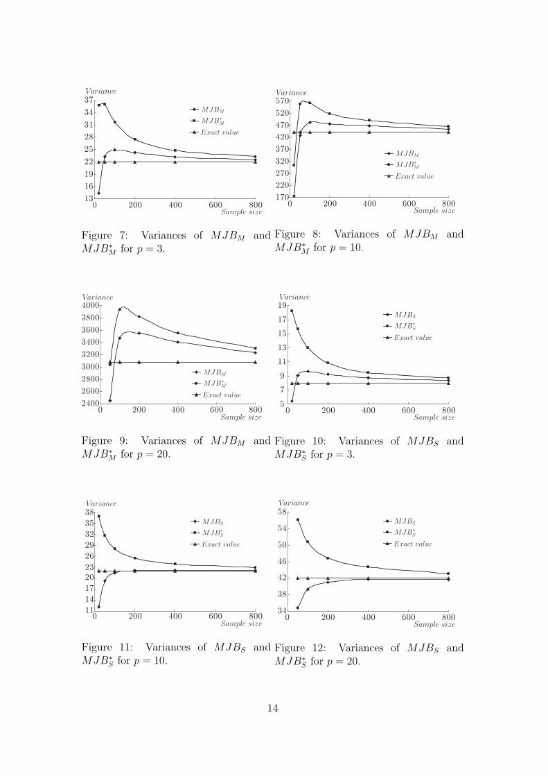
On the other hand, from Tables 1–2 and Figures 7–12, variances of MJB∗M

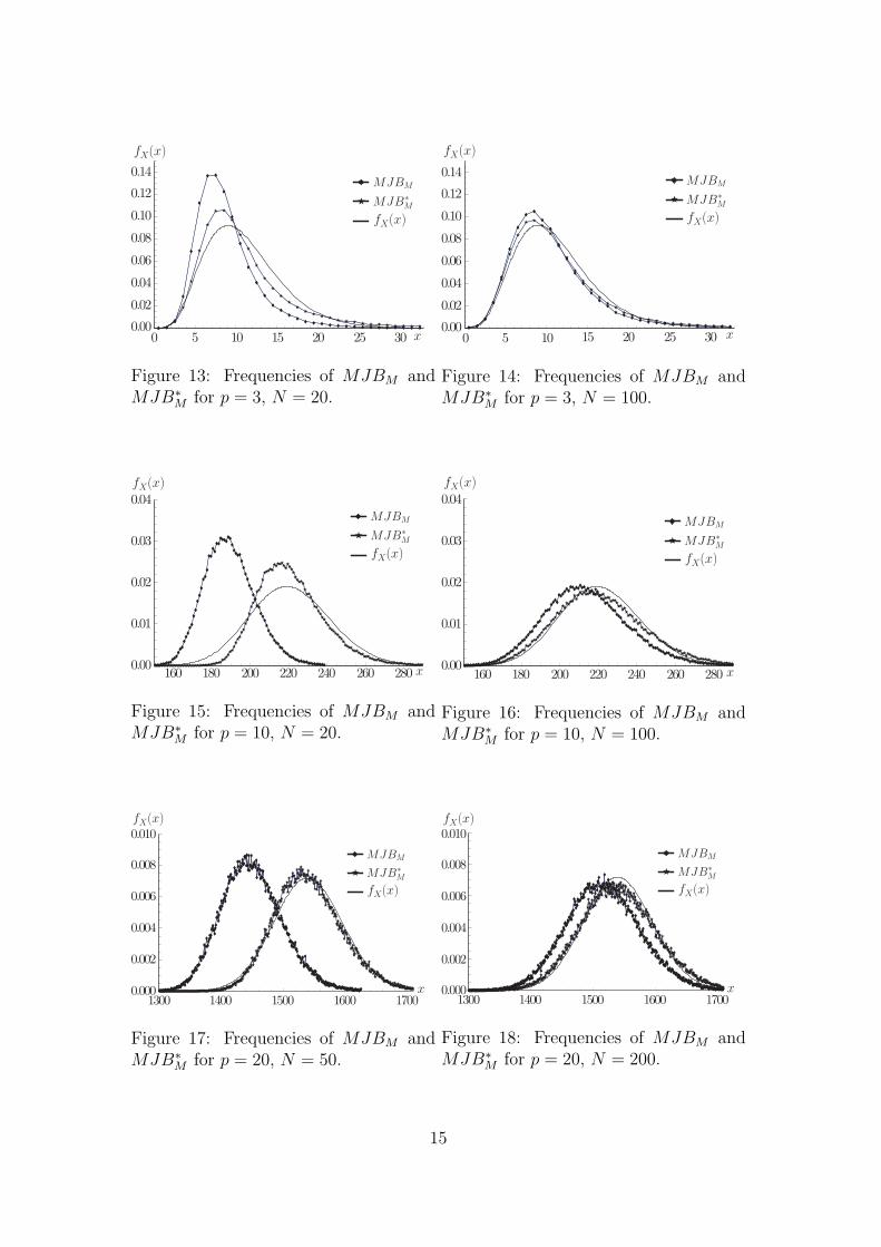
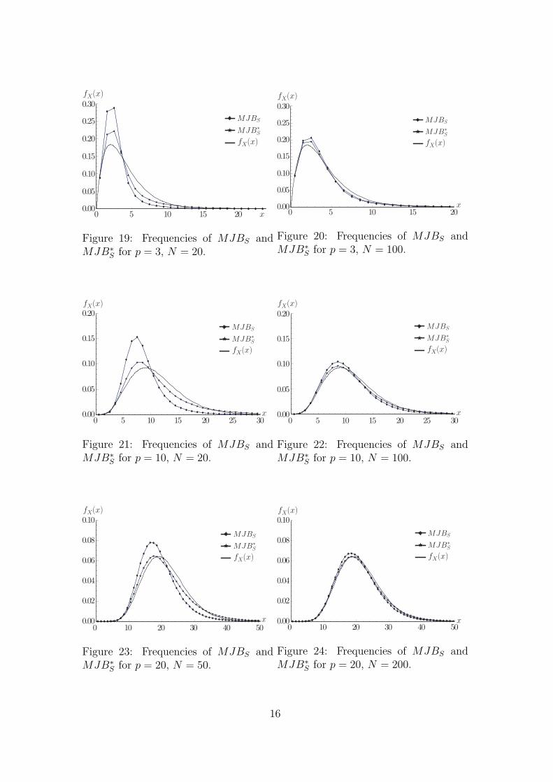
and MJB∗S are larger than those of MJBM and MJBS. To investigate this cause,

we show frequency distributions of multivariate Jarque-Bera tests proposed in this

paper. These results are in Figures 13–24. In figures, fX(x) represents probability

density function (p.d.f.) of χ2-distribution. It may be noticed from these figures

that frequencies of MJB∗M and MJB∗

S are closer to p.d.f. of χ2-distribution than

those of MJBM and MJBS, respectively. This tendency appears well when sample

size N is small. But the coming off values of MJB∗M and MJB∗

S are more than

those of MJBM and MJBS. Therefore there is a tendency for variance to become

large.

Finally, in Table 3 and Figures 25–27, we give upper percentage points of

MJBM and MJB∗M by using Mardia’s skewness and kurtosis. MJBM tends to

be conservative. Also MJB∗M is closer to the upper percentage points of χ2

f+1-

distribution even when the sample size N is small. In Table 4 and Figures 28–30,

we give upper percentage points of MJBS and MJB∗S by using Srivastava’s skew-

ness and kurtosis. We note that the tendency is similar to the case using Mardia’s

moments.

8

5 Concluding remarks

For univariate sample case, Jarque-Bera test is well known as a simple procedure

on practical use. In this paper, we proposed four new test statistics for assessing

multivariate normality. MJBM and MJBS are natural forms of extensions in the

case of multivariate normality tests. But approximations of expectations, frequency

distributions and upper percentage points of MJBM and MJBS are not good when

the sample size N is small. Also we proposed improved multivariate normality

test statistics MJB∗M and MJB∗

S. Hence we improved expectations and upper

percentage points of MJBM and MJBS. But variances of MJBM and MJBS are

not improved. This problem still remains. It is an future problem. In order to solve

this problem, it may be noted that we have to consider covariance of z∗M,1 and z∗2

M,2

and that of z∗S,1 and z∗2

S,2. We recommend to use MJB∗M and MJB∗

S from the aspect

of aproximate accuracy of upper percentage points of test statistics especially for

small N .

References

[1] Jarque, C. M. and Bera, A. K. (1987). A test for normality of observations

and regression residuals. International Statistical Review, 55, 163–172.

[2] Malkovich, J. R. and Afifi, A. A. (1973). On tests for multivariate normality.

Journal of the American Statistical Association, 68, 176–179.

[3] Mardia, K. V. (1970). Measures of multivariate skewness and kurtosis with

applications. Biometrika, 57, 519–530.

[4] Mardia, K. V. (1974). Applications of some measures of multivariate skewness

and kurtosis in testing normality and robustness studies. Sankhya B, 36, 115–

128.

9

[5] Okamoto, N. and Seo, T. (2008). On the Distribution of Multivariate Sample

Skewness for Assessing Multivariate Normality. Technical Report No. 08-01,

Statistical Research Group, Hiroshima University.

[6] Royston, J. P. (1983). Some techniques for assessing multivariate normality

based on the Shapiro-Wilk W. Applied Statistics, 32, 121–133.

[7] Seo, T. and Ariga, M. (2006). On the Distribution of Kurtosis Test for Mul-

tivariate Normality. Technical Report No. 06-04, Statistical Research Group,

Hiroshima University.

[8] Shapiro, S. S. and Wilk, M. B. (1965). An analysis of variance test for normality

(complete samples). Biometrika, 52, 591–611.

[9] Srivastava, M. S. (1984). A measure of skewness and kurtosis and a graphical

method for assessing multivariate normality. Statistics &Probability Letters, 2,

263–267.

[10] Srivastava, M. S. and Hui, T. K. (1987). On assessing multivariate normality

based on Shapiro-Wilk W statistic. Statistics &Probability Letters, 5, 15–18.

[11] Urzua, C. M. (1996). On the correct use of omnibus tests for normality. Eco-

nomics Letters, 90, 304–309.

10

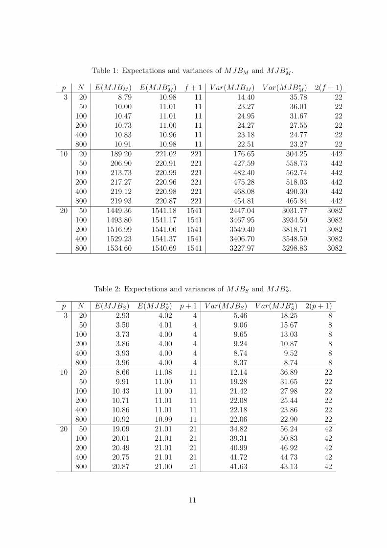
Table 1: Expectations and variances of MJBM and MJB∗M .

p N E(MJBM) E(MJB∗M) f + 1 V ar(MJBM) V ar(MJB∗

M) 2(f + 1)3 20 8.79 10.98 11 14.40 35.78 22

50 10.00 11.01 11 23.27 36.01 22100 10.47 11.01 11 24.95 31.67 22200 10.73 11.00 11 24.27 27.55 22400 10.83 10.96 11 23.18 24.77 22800 10.91 10.98 11 22.51 23.27 22

10 20 189.20 221.02 221 176.65 304.25 44250 206.90 220.91 221 427.59 558.73 442

100 213.73 220.99 221 482.40 562.74 442200 217.27 220.96 221 475.28 518.03 442400 219.12 220.98 221 468.08 490.30 442800 219.93 220.87 221 454.81 465.84 442

20 50 1449.36 1541.18 1541 2447.04 3031.77 3082100 1493.80 1541.17 1541 3467.95 3934.50 3082200 1516.99 1541.06 1541 3549.40 3818.71 3082400 1529.23 1541.37 1541 3406.70 3548.59 3082800 1534.60 1540.69 1541 3227.97 3298.83 3082

Table 2: Expectations and variances of MJBS and MJB∗S.

p N E(MJBS) E(MJB∗S) p + 1 V ar(MJBS) V ar(MJB∗

S) 2(p + 1)3 20 2.93 4.02 4 5.46 18.25 8

50 3.50 4.01 4 9.06 15.67 8100 3.73 4.00 4 9.65 13.03 8200 3.86 4.00 4 9.24 10.87 8400 3.93 4.00 4 8.74 9.52 8800 3.96 4.00 4 8.37 8.74 8

10 20 8.66 11.08 11 12.14 36.89 2250 9.91 11.00 11 19.28 31.65 22

100 10.43 11.00 11 21.42 27.98 22200 10.71 11.01 11 22.08 25.44 22400 10.86 11.01 11 22.18 23.86 22800 10.92 10.99 11 22.06 22.90 22

20 50 19.09 21.01 21 34.82 56.24 42100 20.01 21.01 21 39.31 50.83 42200 20.49 21.01 21 40.99 46.92 42400 20.75 21.01 21 41.72 44.73 42800 20.87 21.00 21 41.63 43.13 42

11

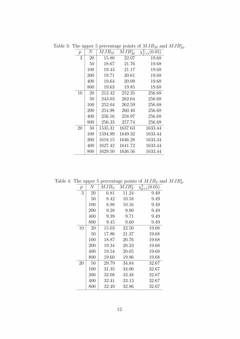
Table 3: The upper 5 percentage points of MJBM and MJB∗M .

p N MJBM MJB∗M χ2

f+1(0.05)

3 20 15.80 22.07 19.6850 18.67 21.76 19.68

100 19.43 21.17 19.68200 19.71 20.61 19.68400 19.64 20.09 19.68800 19.63 19.85 19.68

10 20 212.42 252.35 256.6850 243.03 262.64 256.68

100 252.04 262.59 256.68200 254.98 260.40 256.68400 256.16 258.97 256.68800 256.33 257.74 256.68

20 50 1535.31 1637.63 1633.44100 1594.99 1649.32 1633.44200 1618.15 1646.28 1633.44400 1627.42 1641.72 1633.44800 1629.50 1636.56 1633.44

Table 4: The upper 5 percentage points of MJBS and MJB∗S.

p N MJBS MJB∗S χ2

p+1(0.05)

3 20 6.81 11.24 9.4950 8.42 10.58 9.49

100 8.98 10.16 9.49200 9.28 9.90 9.49400 9.39 9.71 9.49800 9.45 9.60 9.49

10 20 15.03 22.50 19.6850 17.86 21.37 19.68

100 18.87 20.76 19.68200 19.34 20.33 19.68400 19.54 20.05 19.68800 19.60 19.86 19.68

20 50 29.79 34.84 32.67100 31.35 34.06 32.67200 32.08 33.48 32.67400 32.41 33.13 32.67800 32.49 32.86 32.67

12

8.5

9.5

10.5

11.5

0 200 400 600 800Sample size

Expectation

Exact value

MJBM

MJB!M

Figure 1: Expectations of MJBM andMJB∗

M for p = 3.

188

192

196

200

204

208

212

216

220

224

0 200 400 600 800

Expectation

Sample size

Exact value

MJBM

MJB∗M


M for p = 10.

1440

1460

1480

1500

1520

1540

1560

0 200 400 600 800

Expectation

Sample size

Exact value

MJBM

MJB∗M


M for p = 20.

2.9

3.1

3.3

3.5

3.7

3.9

4.1

0 200 400 600 800

Exact value

MJBS

MJB!S

Sample size

Expectation

Figure 4: Expectations of MJBS andMJB∗

S for p = 3.

8.5

9.5

10.5

11.5

0 200 400 600 800Sample size

Expectation

Exact value

MJBS

MJB!S


S for p = 10.

19

19.5

20

20.5

21

21.5

0 200 400 600 800

Expectation

Sample size

Exact value

MJBS

MJB!S


S for p = 20.

13

13

16

19

22

25

28

31

34

37

0 200 400 600 800

Exact value

MJBM

MJB!M

Variance

Sample size

Figure 7: Variances of MJBM andMJB∗

M for p = 3.

170

220

270

320

370

420

470

520

570

0 200 400 600 800

Variance

Exact value

MJBM

MJB!M

Sample size


M for p = 10.

2400

2600

2800

3000

3200

3400

3600

3800

4000

0 200 400 600 800

Variance

Sample size

Exact value

MJBM

MJB!M


M for p = 20.

5

7

9

11

13

15

17

19

0 200 400 600 800

Variance

Sample size

Exact value

MJBS

MJB!S

Figure 10: Variances of MJBS andMJB∗

S for p = 3.

11

14

17

20

23

26

29

32

35

38

0 200 400 600 800

Variance

Sample size

Exact value

MJBS

MJB!S


S for p = 10.

34

38

42

46

50

54

58

0 200 400 600 800

Variance

Sample size

Exact value

MJBS

MJB!S


S for p = 20.

14

0 5 10 15 20 25 300.00

0.02

0.04

0.06

0.08

0.10

0.12

0.14fX(x)

x

MJBM

MJB∗M

fX(x)

Figure 13: Frequencies of MJBM andMJB∗

M for p = 3, N = 20.

0 5 10 15 20 25 300.00

0.02

0.04

0.06

0.08

0.10

0.12

0.14

fX(x)

MJBM

MJB!M

fX(x)

x


M for p = 3, N = 100.

160 180 200 220 240 260 2800.00

0.01

0.02

0.03

0.04fX(x)

x

MJBM

MJB!M

fX(x)


M for p = 10, N = 20.

160 180 200 220 240 260 2800.00

0.01

0.02

0.03

0.04fX(x)

x

MJBM

MJB!M

fX(x)


M for p = 10, N = 100.

1300 1400 1500 1600 17000.000

0.002

0.004

0.006

0.008

0.010fX(x)

x

MJBM

MJB!M

fX(x)


M for p = 20, N = 50.

1300 1400 1500 1600 17000.000

0.002

0.004

0.006

0.008

0.010fX(x)

x

MJBM

MJB!M

fX(x)


M for p = 20, N = 200.

15

0 5 10 15 200.00

0.05

0.10

0.15

0.20

0.25

0.30

x

fX(x)

MJBS

MJB!S

fX(x)

Figure 19: Frequencies of MJBS andMJB∗

S for p = 3, N = 20.

0 5 10 15 200.00

0.05

0.10

0.15

0.20

0.25

0.30

x

fX(x)

MJBS

MJB!S

fX(x)


S for p = 3, N = 100.

0 5 10 15 20 25 300.00

0.05

0.10

0.15

0.20fX(x)

x

MJBS

MJB!S

fX(x)


S for p = 10, N = 20.

0 5 10 15 20 25 300.00

0.05

0.10

0.15

0.20fX(x)

x

MJBS

MJB!S

fX(x)


S for p = 10, N = 100.

0 10 20 30 40 500.00

0.02

0.04

0.06

0.08

0.10fX(x)

x

MJBS

MJB!S

fX(x)


S for p = 20, N = 50.

0 10 20 30 40 500.00

0.02

0.04

0.06

0.08

0.10fX(x)

x

MJBS

MJB!S

fX(x)


S for p = 20, N = 200.

16

15

16

17

18

19

20

21

22

23

0 200 400 600 800

Exact value

MJBM

MJB!M

Upper 5 percentile

Sample size

Figure 25: The upper percentiles ofMJBM and MJB∗

M for p = 3.

210

220

230

240

250

260

270

0 200 400 600 800

Upper 5 percentile

Exact value

MJBM

MJB!M

Sample size


M for p = 10.

1530

1550

1570

1590

1610

1630

1650

0 200 400 600 800

Upper 5 percentile

Sample size

Exact value

MJBM

MJB!M


M for p = 20.

6.5

7.5

8.5

9.5

10.5

11.5

0 200 400 600 800

Upper 5 percentile

Sample size

Exact value

MJBS

MJB!S

Figure 28: The upper percentiles ofMJBS and MJB∗

S for p = 3.

15

16

17

18

19

20

21

22

23

0 200 400 600 800

Exact value

MJBS

MJB!S

Upper 5 percentile

Sample size


S for p = 10.

29

30

31

32

33

34

35

0 200 400 600 800

Exact value

MJBS

MJB!S

Sample size

Upper 5 percentile


S for p = 20.

17

Documents

On Jarque-Bera tests for assessing multivariate normality