ISS

N 0

249-

6399

ISR

N IN

RIA

/RR

--42

69--

FR

+E

NG

appor t de r echerche

THÈME 1

INSTITUT NATIONAL DE RECHERCHE EN INFORMATIQUE ET EN AUTOMATIQUE

On fairness in Bandwidth Allocation

Corinne Touati, Eitan Altman, Jérôme Galtier

N° 4269

Septembre 2001

Unité de recherche INRIA Sophia Antipolis2004, route des Lucioles, BP 93, 06902 Sophia Antipolis Cedex (France)

Téléphone : +33 4 92 38 77 77 — Télécopie : +33 4 92 38 77 65

On fairness in Bandwidth Allocation

Corinne Touati, Eitan Altman, Jérôme Galtier

Thème 1 � Réseaux et systèmesProjet Mistral, Mascotte

Rapport de recherche n° 4269 � Septembre 2001 � 23 pages

Abstract: For over a decade, the Nash bargaining solution (NBS) concept from cooperative gametheory has been used in networks as a concept that allows one to share resources fairly. Due to itsmany appealing properties, it has recently been used for assigning bandwidth in a general topologynetwork between applications that have linear utilities. In this paper, we use this concept for thebandwidth allocation between applications with general concave utilities. We study the impact ofconcavity on the allocation and present computational methods for obtaining fair allocations in ageneral topology, based on a dual Lagrangian approach and on Semi-De�nite Programming.

Key-words: Nash Bargaining, bandwith allocation, fairness

La notion d'équité dans l'allocation de bande passante

Résumé : Le concept de Nash Bargaining Solution (NBS), né de la théorie des jeux coopératifs,est utilisé depuis plus de dix ans dans les réseaux pour permettre le partage équitable des ressources.Grâce à ses propriétés intéressantes, il a récemment été utilisé dans des problèmes d'allocation debande passante dans des réseaux aux topologies quelconques où se côtoient des applications auxfonctions d'utilité linéaires. Dans cet article, nous utilisons le NBS dans le cadre de l'allocationde bande passante entre des applications aux fonctions d'utilités concaves quelconques, étudionsl'impact de la concavité sur l'allocation et présentons des méthodes calculatoires pour obtenir desallocations équitables dans une topologie générale, basées sur une approche de dual Lagrangien etde programmation semi-dé�nie.

Mots-clés : équité, allocation de bande passante, Nash Bargaining

Contents

1 Introduction 4

2 General problem 4

2.1 Utility function . . . . . . . . . . . . . . . . . . . . . . . . . . . . . . . . . . . . . . . 42.2 Fair allocations . . . . . . . . . . . . . . . . . . . . . . . . . . . . . . . . . . . . . . . 52.3 Statement of the general problem . . . . . . . . . . . . . . . . . . . . . . . . . . . . . 7

3 Properties of the NBS and of GPF 8

3.1 An example with linear utilities . . . . . . . . . . . . . . . . . . . . . . . . . . . . . . 83.2 The impact of concavity . . . . . . . . . . . . . . . . . . . . . . . . . . . . . . . . . . 8

4 Quadratic utility functions 10

4.1 De�nition of the utility function . . . . . . . . . . . . . . . . . . . . . . . . . . . . . . 104.2 The linear network example . . . . . . . . . . . . . . . . . . . . . . . . . . . . . . . . 114.3 Grid network . . . . . . . . . . . . . . . . . . . . . . . . . . . . . . . . . . . . . . . . 14

5 Lagrangian method 14

5.1 Lagrangian multipliers . . . . . . . . . . . . . . . . . . . . . . . . . . . . . . . . . . . 155.2 Dual problem . . . . . . . . . . . . . . . . . . . . . . . . . . . . . . . . . . . . . . . . 165.3 Decentralized implementation . . . . . . . . . . . . . . . . . . . . . . . . . . . . . . . 16

6 An SDP solution 17

6.1 Properties of positive semi-de�nite matrices . . . . . . . . . . . . . . . . . . . . . . . 176.2 Computing the NBS and GPF . . . . . . . . . . . . . . . . . . . . . . . . . . . . . . . 186.3 A simple example . . . . . . . . . . . . . . . . . . . . . . . . . . . . . . . . . . . . . . 196.4 Practical experiments . . . . . . . . . . . . . . . . . . . . . . . . . . . . . . . . . . . 20

7 Conclusion 22

RR n° 4269

1 Introduction

Fair bandwidth assignment has been one of the important challenging areas of research and devel-opment in networks supporting elastic tra�c. Indeed, Max-min fairness has been adopted by theATM forum for the Available Bit Rate (ABR) service of ATM [1]. Although the max-min fairnesshas some optimality properties (Pareto optimality), it has been argued that it favors too muchlong connections and does not make e�cient use of available bandwidth. In contrast, the conceptof proportional fairness (of the throughput assignment) has been proposed by Kelly [11, 7], whichgives rise to a more e�cient solution in terms of network resources by providing more resources toshorter connections. An assignment is proportionally fair if any change in the distribution of theassigned rates would result in the sum of the proportional changes to be non-positive.

Although the object that is shared fairly seems to be a very speci�c one: the throughput, itis shown in [11, 7] that in fact, the starting point for obtaining (weighted) proportional fairnessof the throughput can be a general (concave) utility function per connection; it is then shownthat a global minimization of (weighted) sum of these utilities leads to a weighted proportional fairassignment of the throughput. As opposed to this approach, we wish to use a fairness concept whichis de�ned directly in terms of the utilities of users rather than in terms of the throughputs they areassigned. Yet, as in weighted proportional fairness, it would be desirable to obtain this concept asthe solution of a utility maximization problem, since it makes it possible to use recent algorithmsfor utility maximization in networks, along with decentralized implementations [10, 9, 12].

NBS is a natural framework that allows us to de�ne and design fair assignment of bandwidthbetween applications with di�erent concave utilities and has already been used in networking prob-lems [14, 8]. It is characterized by a set of axioms that are appealing in de�ning fairness. As alreadyrecognized in [7] and later in [8], proportional fairness agrees with NBS in case that the object thatis shared fairly is the throughput (and the minimum required rate is zero). We use NBS to studythe fairness of an assignment where connection i has a concave utility over an interval [MRi; PRi].It thus has a minimum rate requirement MRi and does not need more than PRi. Utility functionswith similar features have been identi�ed in [17] for representing some real time applications suchas voice and video, and in the case that MRi = 0, for elastic tra�c.

We study in this paper the way the concavity of the utilities a�ect the bandwidth assignmentaccording to NBS, as well as according to a generalized version of the proportional fairness (inwhich the utilities that correspond to di�erent assignments, instead of the throughputs, are fairlyallocated). Both notions are introduced in Sec. 2 and their properties are studied in Sec. 3. Wethen propose in Sec. 4 a quadratic approximation for the utility of each connection, which allows usto parameterize the degree of concavity of the utility function using a single parameter. We use thisapproximation to further analyze the impact of concavity of utilities on the resulting assignment.We then present in Sec. 5 a Lagrangian approach which allows us to implement a decentralizedprotocol for the bandwidth allocation. We �nally present in Sec. 6 a novel alternative approachusing Semi De�nite Programming (SDP).

2 General problem

2.1 Utility function

The fairness problem which we consider is how to allocate bandwidth to connections beyond theirminimum required bandwidth (MR). (We assume that if the minimum required bandwidth is notavailable then the connection is not accepted by the network.) The fairness issue is of interest only

INRIA

in the case when the utility of an application strictly increases when allocated more bandwidth thanits MR. Connections with on/o� utility functions (which characterize some applications with hardreal-time requirements, [17]) are thus ignored in allocating extra bandwidth once they receive theirMR.

Two kinds of applications are considered in [17] for which the fair allocation is relevant:

Elastic applications: Examples of such applications are �le transfer or email. The typical utilityfunction is concave increasing without a required minimum rate, see Fig. 1.

Rate / Delay adaptive ApplicationsMR

Elastic Applications

U

Bandwith Bandwith

U

Figure 1: Utility function of elastic (left) and of rate-adaptive or delay-adaptive (right) applications

�Delay adaptive� or �rate adaptive� applications: These are typically real time applications such asvoice or video over IP. The utility functions that we use for these applications (Fig. 1) are slightlydi�erent than those in [17]. In [17], the utility is always strictly positive for non null bandwidthand tends to zero when the bandwidth does. We consider in contrast that the utility equals zerobelow a certain value, as in [8]. Indeed, in many voice applications, one can select the transmissionrate by choosing an appropriate compression mechanism and existing compression software have anupper bound on the compression, which implies a lower bound on the transmission rate for which acommunication can be initiated. If there is no su�cient bandwidth, the connection is not initiated.This kind of behavior generates utility functions that are zero for bandwidth below MR and whichare not di�erentiable at the point (MR; 0).

2.2 Fair allocations

Several concepts of fairness are known in the literature: the max-min fairness [3], (as well as themore general concept of weighed max-min fairness) which has been adopted by the ATM-forum [1]for ABR tra�c, the proportional fairness [7] the harmonic mean fairness [13], the general fairnesscriterion that bridges all the above concepts [15] and the Nash Bargaining Solution (NBS).Nash Bargaining Solution (NBS) Our starting point is the NBP (Nash Bargaining Point) concept [8]for fair allocation, frequently used in cooperative game theory. Let there be n users (or connections).The notion deals directly with fair allocation of achievable utilities of players (and does not requireto relate them to the original objects, throughputs in our case, that generate these utilities). LetU � IRn be a closed convex set corresponding to the achievable vectors of utilities of the form(f1; :::; fn). Let u

0i be a minimum required performance of user i.1 Let G = f(U; u0)jU � IRng: it

denotes the class of sets of performance measures that satisfy the minimum performance bound u0

(it contains achievable performances obtained for di�erent utility functions f ; in fact, in order tode�ne NBP one has to introduce its performance w.r.t. other utilities, as is seen from property 3and 5 in the de�nition below).

1In our context, u0i = fi(MRi) where fi is concave increasing. If X is the set of all achievable vectors of bandwidths,then U = ff(x)jx 2 Xg.

RR n° 4269

De�nition 2.1. A mapping S : G ! IRn is said to be an NBP (Nash bargaining point) if

1. S(U; u0) 2 U0 := fu 2 U ju � u0g, i.e. it guarantees the minimum required performances.

2. It is Pareto optimal 2.

3. It is linearly invariant, i.e. the bargaining point is unchanged if the performance objectives area�nely scaled. More precisely, if � : IRn ! IRn is a linear map such that its ith componentis given by �i(u) = aiui + bi, then S(�(U); �(u0)) = �(S(U; u0)).

4. S is symmetric i.e. does not depend on the speci�c labels, i.e. users with the same minimumperformance measures and the same utilities will have the same performances.

5. S is not a�ected by enlarging the domain if a solution to the problem with the larger domaincan be found on the restricted one. More precisely, if V � U , (V; u0) 2 G, and S(U; u0) 2 Vthen S(U; u0) = S(V; u0).

The de�nition of NBP is thus given through axioms that game theorists �nd natural to require inseeking for fair assignment. Having de�ned this concept through the achievable utilities, we de�nethe NBS (Nash Bargaining Solution) in terms of the corresponding strategies (i.e. the allocationof bandwidth that results in the NBP), and then present its characterization through a utilityoptimization approach.

De�nition 2.2. The point u� := S(U; u0) is called the Nash Bargaining Point and f�1(u�) is calledthe set of Nash Bargaining Solutions.

De�ne X0 := fx 2 Xjf(x) � u0g.Theorem 2.1. [8, Thm. 2.1, Thm 2.2]. Let the utility functions fi be concave, upper-bounded, de-�ned on X which is a convex and compact subset of L. Let J be the set of users able to achieve a per-formance strictly superior to their initial performance, i.e. J = fj 2 f1; :::; ngj9x 2 X0; s:t: fj(x) >u0jg. Assume that ffjgj2J are injective. Then there exists a unique NBP as well as a unique NBSx that veri�es fj(x) > uj(x); j 2 J , and is the unique solution of the problem PJ :

(PJ) maxYj2J

(fj(x)� u0j); x 2 X0: (1)

Equivalently, it is the unique solution of:

(P 0J) max

Xj2J

ln(fj(x)� u0j); x 2 X0:

Before examining some qualitative implications of the de�nition, we introduce the very relatednotion of generalized proportional fairness.Generalized proportional fairness (GPF). An assignment x 2 X is said to be (generalized) pro-portionally fair with respect to a utility f , if for any other assignment x� 2 X, the aggregate ofproportional changes in the utilities is zero or negative

nXi=0

fi(x�i )� fi(xi)

fi(xi)� 0: (2)

2An allocation f is said to be Pareto optimal if it is impossible to strictly increase the allocation of a connectionwithout strictly decreasing another one. The Pareto axiom assures that no bandwidth is "wasted".

INRIA

Thus, an allocation is GPF if any change in the distribution of the rates would result in the sumof the proportional changes of the utilities to be non-positive. This concept has been de�ned andapplied without considering any utility, i.e. by restricting directly the rates as the object that isassigned fairly [11, 7] (see also [4, 13, 15]). This amounts in taking in (2) fi(xi) = xi. Yet, there isno conceptual di�erence in de�ning it as we do, i.e. with respect to utilities. In particular, by simplyreplacing xi by fi(xi), we have the following property (established for the special case fi(xi) = xi)of the solution xGPF :

xGPF maximizes

nXi=1

ln fi(xi) over X (3)

or xGPF maximizesnYi=1

fi(xi) over X. (4)

The Internet is an example where proportional fairness is used. Indeed, congestion control mech-anisms based on linear increase and multiplicative decrease (such as TCP) achieve proportionalfairness upper appropriate conditions [7]. The (weighted version of the) proportional fairness is alsoadvocated for future developments of TCP [6].

Comparing with Thm. 2.1, we conclude that GPF coincides with the NBS of [8] when theMRi'sequal zero, and to the original proportional fairness when further restricting to the identity utilities.

We �nally note that due to (4) it follows that GPF is invariant under a scale change, i.e. ifwe multiply the utility fi of a connection i by a positive constant ci, the GPF assignment will notchange. Yet in general, it will not remain the same under translation by a constant as in NBS.General fairness criterion. We present another general fairness criterion [15] but apply it to fairallocation of utilities rather than of the rate. Given a positive constant � 6= 1, consider the problem

maxx

1

1� �

nXi=1

fi(xi)1��; � � 0; � 6= 1: (5)

subject to the problem's constraints. This de�nes a unique allocation which is called the �-bandwidth allocation. This allocation corresponds to the globally optimal allocation as � ! 0,to the (generalized) proportional fairness when � ! 1, to the generalized harmonic mean fairnesswhen �! 2, and to the generalized max-min allocation when �!1 [15]. We shall not deal withthis concept until Sec. 6.

2.3 Statement of the general problem

We focus in the paper on the computation of the NBS and brie�y compare it to the GPF allocation.Using Thm. 2.1, the NBS is the unique solution x = x1; x2; :::; xn (with n the number of connections)of

maxx2X

nYi=1

(fi(xi)� fi(MRi)) where Xi :=

fxj8l = 1; :::; L; (Ax)l � (C)l;MRi � xi � PRig;(6)

with L the number of links, A the routing matrix (the element Ai;j being equal to 1 if connection jgoes through link i, 0 otherwise), and C the capacity vector (Ci is the capacity of link i). (Ax)l �(C)l are the standard capacity constraints. We assume that the network has su�cient bandwidthto satisfy all the users' minimum requirements i.e. 8 2 1::L we have

PNi=1 aliMRi < Cl.

RR n° 4269

3 Properties of the NBS and of GPF

As already mentioned, previous references that studied proportional fairness considered the actualbandwidth as the object to be allocated fairly, rather than its utility. The reference [8] who alreadyconsidered the NBS approach which is de�ned for general concave utilities, also restricted to linearutilities. Our �rst goal is thus to study utilities that are more general than those already studiedin the following aspects:(1) allow general concave utilities,(2) allow fi(MRi) to be di�erent from zero.

We note that due to the 3rd axiom in the de�nition of NBP (Def. 2.1), the second point abovewill not a�ect the NBP (and the NBS) but will a�ect the GPF allocation.

3.1 An example with linear utilities

Consider two connections with the same PRi and MRi (we thus omit the index i) that competeover a single link with capacity cap satisfying 2PR > cap > 2MR. The utility of connection i isfi(x) = ai(x � Zi), ai > 0, Zi � MR. Without loss of generality, we assume that a = ai does notdepend on i, since both the NBS as well as GPF are scale invariant. The NBS is clearly x�i = cap=2,i = 1; 2. De�ne

Yi =cap

2+Zi � Zj

2; j 6= i

A simple calculation shows that the GPF solution is xGPFi = Yi if Yi 2 [MRi; PRi], and if not, thenfor some i, Yi < MRi. In that case, the GPF solution is xGPFi = Yi and xGPFj = cap �MRi, forj 6= i.

This example shows that if we translate the utility of connection i by a positive constant (whichimplies that Zi decreases) then its generalized fair share decreases whereas its NBS share does notchange.

3.2 The impact of concavity

We now study the impact of concavity on the NBS. Consider two di�erentiable functions f and gde�ned on the same interval [MR;PR] where both are strictly positive on (MR;PR]. We say that fis more concave than g if for every x 2 (MR;PR], the relative derivative of f is smaller than or equalto that of g, i.e. f 0(x)=f(x) � g0(x)=g(x) (if f or g were not di�erentiable at x, one could requireinstead that the same relation holds for the supergradients: if f(x) is the largest supergradient off at x and g(x) is the smallest supergradient of g at x, then we require f(x)=f(x) � g(x)=g(x)).

Motivated by (4), we say that an assignment x is more fair in the sense of GPF than anassignment y if

Qni=1 fi(xi) �

Qni=1 fi(yi): One can de�ne similarly an ordering for the NBS fairness,

but then one has to replace fi by fi � fi(MRi).In the next example we consider the case in which fi(MRi) = 0 (so NBS coincides with GPF).

Consider 2 connections with utilities f and g as above competing for the bandwidth of a single link.If we had ignored the utilities of the connections, we would have assigned them an equal bandwidth(according to the original proportional allocation), which we denote by x = cap=2. We show thatby transferring bandwidth from the connection with the more concave utility (say f) to the otherone, we improve the fairness (assuming this does not violate the MR and PR constraints) in the

INRIA

sense of GPF or the NBS. Indeed, we have

g(x + �)f(x� �)

= g(x)f(x)

�1 + �

�g0(x)

g(x)� f 0(x)

f(x)

�+ o(�)

�

where o(�) is a function that tends to zero when divided by � as � converges to zero. We concludethat there is some �0 s.t. for all � < �0, g(x+ �)f(x� �) > g(x)f(x). Hence we strictly improve thefairness by transferring an amount of �0 to the connection with less concave utility.

By further increasing the amount we transfer, we shall eventually reach a local maximum (sinceour function is continuous over a compact interval). This will be a global maximum since (4) isa problem of maximization of a concave function over a convex set. We conclude that the fairassignment has the property that more bandwidth is assigned to the less concave function.Example: Let f(x) = 3x1f0 � x � 1g + (2 + x)1fx > 1g, and let g(x) = 2x for x � 0. Thenf 0(x)=f(x) = x�1 for x 2 [0; 1), and (2 + x)�1 for x � 1, whereas g0(x)=g(x) = x�1 everywhere.(At x = 1, f is not di�erentiable but its supergradients at that point is the set [1=3; 1]). Thus f ismore concave than g. We assume that PR > cap.

De�ne h(x) = 6x(cap� x) and k(x) = 2(x+ 2)(cap� x). The NBS or GPF are obtained as theargument of �(cap) = max f(x)g(cap� x) which equals

max�

maxx2[0;1]

h(x);maxx>1

k(x)�:

If cap > 2 then maxx2[0;1] h(x) = h(1) = 6(cap � 1), otherwize it is obtained at x = cap=2 andequals 3cap2=2.If cap < 4 then maxx>1 k(x) = k(1) = 6(cap� 1), otherwize it is obtained at 1 + cap=2 and equals2(1 + cap=2)2.

0 42

x2x1

x

Cap

3

1

Figure 2: NBS for two connections sharing a link.

The NBS is depicted in Fig 2. We distinguish 3 regions.(i) cap < 2, where �(cap) = 3cap2=2 and the NBS is x�1 = cap=2.(ii) 2 � cap < 4, where �(cap) = 6(cap� 1) and x�1 = 1.(iii) cap � 4, where �(cap) = 2(1 + cap=2)2 and x�1 = cap=2� 1.

The other connection receives in all cases x�2 = cap � x�1. We see in this example that indeedthe least concave function receives at least as much as the other one, and the di�erence increaseswith cap. It's impressive to note that there is a region in which an increase in the capacity bene�tsonly for one connection. The example illustrates the power of the NBS (or GPF) approach: theoriginal proportional fairness, or even weighted proportional fairness, would assign a proportion of

RR n° 4269

the capacity to each connection that does not vary as we increase the capacity, since it is insensitiveto the utilities. In contrast, utility sensitive fairness concepts allocate the bandwidth in a dynamicway: the proportion assigned to each connection is a function of the capacity.

4 Quadratic utility functions

4.1 De�nition of the utility function

MR PR

T

fPR

Figure 3: Quadratic utility function.

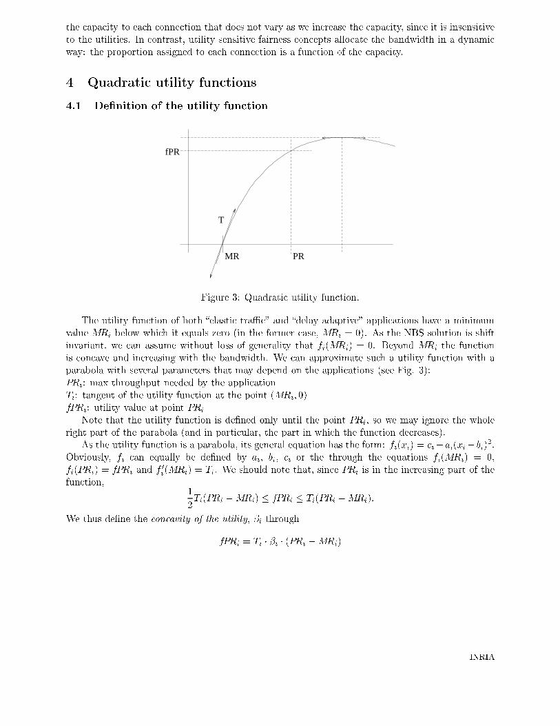
The utility function of both �elastic tra�c� and �delay adaptive� applications have a minimumvalue MRi below which it equals zero (in the former case, MRi = 0). As the NBS solution is shiftinvariant, we can assume without loss of generality that fi(MRi) = 0. Beyond MRi the functionis concave and increasing with the bandwidth. We can approximate such a utility function with aparabola with several parameters that may depend on the applications (see Fig. 3):PRi: max throughput needed by the applicationTi: tangent of the utility function at the point (MRi; 0)fPRi: utility value at point PRi

Note that the utility function is de�ned only until the point PRi, so we may ignore the wholeright part of the parabola (and in particular, the part in which the function decreases).

As the utility function is a parabola, its general equation has the form: fi(xi) = ci�ai(xi� bi)2:

Obviously, fi can equally be de�ned by ai, bi, ci or the through the equations fi(MRi) = 0,fi(PRi) = fPRi and f 0i(MRi) = Ti. We should note that, since PRi is in the increasing part of thefunction,

1

2Ti(PRi �MRi) � fPRi � Ti(PRi �MRi):

We thus de�ne the concavity of the utility, �i through

fPRi = Ti � �i � (PRi �MRi)

INRIA

We have: 1=2 � �i � 1 and the smaller �i is, the more concave is the utility. The limit �i = 1 isthe linear case (studied in [8]). And therefore:

ai = Ti1� �i

PRi �MRi; bi =

PRi � (2�i � 1)MRi

2(1 � �i)

ci =Ti4

PRi �MRi

1� �i:

We next present several examples where we use our parabolic utility functions.

4.2 The linear network example

We consider the problem in Fig. 4 in which the squares represent the links and the lines representthe routes. We have N = L+1 connections sharing L links. Connection 0 uses all the links, whereaseach of the other L connections only goes through a single link (connection i uses link i).

XLX2 X3X1

X0

Figure 4: A linear network.

To obtain the NBS, we need to maximizeYi2f0;:::;Lg

fi(xi): (7)

But, as NBS is Pareto optimal, we have the following constraints for i = 1; :::; L: x0 + xi = Ci as

well as MRi � xi � PRi. This implies bi �q

ciai� xi � bi:

We make two signi�cant assumptions. First, that each link has the same capacity cap. Therefore,it is straightforward to notice that each connection i with 1 � i � L will get the same bandwidthat the equilibrium point. Secondly, we suppose that each of these connections has the same utilityfunction: 8i 2 f2; : : : ; Lg; ai = a1; bi = b1; ci = c1:

Therefore the term to maximize in equation (7) becomes: f0(x)(f1(cap � x))L if we denote byx the throughput of the connection x0.

Solution of the linear problem. By di�erentiating (7) we then obtain:

a0(x� b0)(c1 � a1(cap� x� b1)2) =

La1(cap� x� b1)(c0 � a0(x� b0)2) (8)

which is a polynomial of the third degree. This can be explicitly solved.Possible limits. We are interested in the possible limits xlim of the bandwidth assigned to con-

nection x0 as L grows to in�nity.

Lemma 4.1. Assume MR0 +PR1 � cap. As L grows to in�nity, the only possible limit xlim of thebandwidth assigned to connection x0 is

x(3)lim = b0 �

pc0=a0 = MR0; (9)

RR n° 4269

Proof: Equation (8) shows that since x is bounded, the left part of the equation is boundedtoo. Therefore, the limit xlim, if any, is such that:

a1(cap� xlim � b1)(c0 � a0(xlim � b0)2) = 0 (10)

Since MR0 +PR1 � cap and PR1 � b1, we obtain cap� b1 < MR0 so that the solution is infeasible.

The second solution, x(2)lim = b0 +

pc0=a0 is infeasible as well since we have

b0 +

rc0a0

= PR0 + fPR0PR0 �MR0

2 � (1� �0)

so that this solution is larger than PR0. The last possible solution is (9), which establishes theproof.

It is interesting to note that the limit xlim does not depend on any parameter of the ith(i � 1)connections, or any parameter related to the concavity of the utility function of the connection 0.We show in Fig. 5 how the system converges to the solution as L grows.

10

15

20

25

30

35

40

45

50

10 20 30 40 50 60 70 80 90 100

thro

ughp

ut o

f con

nect

ion

0

Number of links

Influence of the concavity on the equilibrium value MR=10, PR=90, cap=100, fPR=200

T=3T=4T=5

linear case

Figure 5: NBS for the linear network.

Remark 4.1. The condition MR0 +PR1 � cap in Lemma 4.1 (and in the next propositions) is notrestrictive. If it does not hold then we can replace (for any L) MR0 by MR00 := cap� PR1 withouta�ecting the NBS, and then apply Lemma 4.1 for MR00. Indeed, let x� be NBS for the originalproblem. Then x� �MR00 due to the Pareto optimality of the NBS (2nd element in De�nition 2.1).Then it is the NBS for the new problem due to the 5th element in De�nition 2.1.

Asymptotic Analysis. We further re�ne the analysis of the limit as L becomes large, show thatit exists and obtain the rate at which x converges to xlim.

INRIA

Proposition 4.1. Suppose that MR0 + PR1 � cap, then x veri�es:

x = MR0 + Z + o(1=L) (11)

with:

Z =cap�MR0 �MR1

2L

�1� PR1 �MR1

denom

�;

denom = 2(1� �1)(cap�MR0)�PR1 +MR1(2�1 � 1)

where o(1=L) is a function that, when divided by L, tends to zero as L grows to in�nity.

Proof: We shall examine eq. (8) when we substitute x = x(L), which is the solution for a�xed L. As L!1, the left hand side tends to a constant:

limL!1

a0(x� b0)(c1 � a1(cap� x� b1)2) = (12)

�pa0c0�c1 � a1(cap� b1 � b0 +

pc0=a0)

2�:

We now examine the right hand side of (8). It can be written as

La1(cap� x� b1)(c0 � a0(x� b0)2)

= Lf(x)pa(x�MR0) (13)

where f(x) is given bya1(cap� x� b1)(

pc0 �pa0(x� b0))

pa0 (14)

and when substituting x = x(L),

limL!1

f(x) = 2a1(cap� b1 � b0 +pc0=a0)

pa0c0: (15)

Combining (12)-(15), we conclude that

limL!1

L(x(L)�MR0) =

�pa0c0

�c1 � a1(cap� b1 � b0 +

pc0=a0)

2�

2a1(cap� b1 � b0 +pc0=a0)

pa0c0

which yields (11) by substituting the appropriate expressions.We can notice that:

� the convergence of x is in 1=L,

� the result does not depend on T0 nor T1 (scale invariant),

� in the asymptote, none of the parameters of the 0th connection but MR0 appears, so that theresults are independent of the shape of the utility function of x0,

� the larger �1 is, the smaller x gets. This agrees with the conclusions of Subsection 3.2.

In (11), we can easily check the asymptotes for special cases:

� When �1 ! 1 we obtain: Z =cap�MR0 �MR1

L(linear case).

� When �1 ! 1=2 we get: Z =

cap�MR0 �MR1

2L

�1� PR1 �MR1

cap�MR0 � PR1

�:

RR n° 4269

4.3 Grid network

This network is the natural generalization of the linear network. It consists of K �L capacity linkswith K horizontal routes and L vertical routes as shown in Fig. 6.

XL+K

XL+3

XL+2

L+1X

L321X XX X

Figure 6: A grid network.

We suppose that all the horizontal connections have the same utility function fh and each verticalconnection has the utility fv.We can then conclude easily that all the horizontal connections willget the same throughput x and each vertical connection will get the same throughput xv = cap�x.

As in the previous example, we suppose also that, for each i 2 f1; : : : Lg,j 2 f1; : : : Kg, MRi +PRL+j � Ci;L+j and PRi +MRL+j � Ci;L+j.

We then wish to maximize:Yi2[0:L]

fi(xi) = (fh(x))K � (fv(cap� x))L: (16)

Proposition 4.2. In the grid network, x veri�es: x = MRh + Z + o(K=L) with:

Z = K � cap�MRh �MRv

2L

�1� PRv �MRv

denom

�

with denom = 2(1 � �v)(cap�MRh)�PRv +MRv(2�v � 1):

A particular case occurs when L = K and when fh = fv: we obtain x = cap=2.

Proof: This is similar to maximizing: (fh(x)) � (fv(cap � x))L=K . And then, this problem isequivalent to previous case by substituting L=K instead of L. The second assumption is obvious.

5 Lagrangian method

The Lagrangian method was proposed by [8] to obtain NBS for the special case of linear utilityfunction. It has the advantage of having distributed implementations. We generalize below thisapproach to the quadratic utility, for which the linear case can be recovered by taking � ! 1.

INRIA

5.1 Lagrangian multipliers

We now use the Kuhn Tucker conditions for (6) to obtain alternative characterization of the NBSin terms of the corresponding Lagrange multipliers.

Proposition 5.1. Under the hypothesis that 8i 2 f1::Lg;P aliMRi < Cl, the NBS is characterizedby:9�l � 0; l 2 f1::Lg such that 8i 2 f1::Ng; we have

xi = min�PRi;MRi +

LXl=1

�lal;i

!�1

+1

2� PRi �MRi

1� �i�2

6641�vuuuut1 +

4�

1��iPRi�MRi

�2�PL

l=1 �lal;i

�23775�

Proof: Under the assumptionP

aliMRi < Cl, the set A of possible solutions of (6) is non-empty, convex and compact. The constraints in (6) are linear in xi and f(x) is C1, therefore the�rst order Kuhn-Tucker conditions are necessary and su�cient for optimality. The Lagrangianassociated with (6) is

L(x; �; Æ; �) = f(x)�nXi=1

�i(MRi � xi)

�NXi=1

Æi(xi � PRi)�LXl=1

�l((Ax)l � Cl):

For i = 1; :::; n, �i � 0 are the Lagrange multipliers associated with the constraints xi � MRi andÆi � 0 are those associated with the constraints xi � PRi. �l � 0; l = 1:::; L are the Lagrangemultipliers associated with the capacity constraints. The �rst order optimality conditions are thus:8i 2 f1; :::; Ng,

0 = (�i � Æi �LXl=1

�l((Ax)l � Cl))

+fi(x)

fi(xi)� fi(MRi)

@fi(xi)

@xi

and 8i; (xi�MRi)�i = 0; (xi�PRi)Æi = 0, 8l; ((Ax)l�Cl)�l = 0. Moreover,P

aliMRi < Cl impliesthat 8i; �i = 0 as in [8], and either xi = PRi or Æi = 0, which yields the conclusion.

As � ! 1 we obtain the solution of [8] corresponding to linear utility:

xi = min

0@PRi;MRi +

"LXl=1

�lal;i

#�11A :

�l represent the implied cost associated with the network link l. It represents the marginal cost ofa rate unit allocated for any connection crossing link l.

RR n° 4269

5.2 Dual problem

Once we have explicitly expressed the NBS in terms of the Lagrange multipliers, we can actuallysolve the NBS completely using the dual problem in which we compute the Lagrange multipliers.De�ne

gi(p) =

8>>>>>>>>>><>>>>>>>>>>:

PRi if p � 2�i � 1

�i

1

PRi �MRi

MRi +1

p+

1

2

PRi �MRi

1� �i

�"1�

r1 + 4

p2��

1��iPRi�MRi

�2#

otherwise.

Then: xi(�) = gi(LXl=1

�l � al;i): (17)

The dual problem is :

max�2 IRL

+d(�)

with d(�) = minx2X L(x; �) = L(xi; �)(18)

if we note xi the optimal value. The vector x = x1; x2:::xn is the NBS. We obtain for each � 2 IRL:

d(�) =

NXi=1

h� ln(fi(gi(

l2[1::L]Xal;i=1

�l))+

� l2[1::L]Xal;i=1

�l

�gi

� l2[1::L]Xal;i=1

�l

�i LXl=1

Cl�l:

As in [8], there is no duality gap.

5.3 Decentralized implementation

The dual problem gave an alternative centralized optimization problem for computing the NBS.Still, we can use the decentralized implementation from [8] for the computation, where L localalgorithms run at the di�erent nodes. The link updates require information on connections thatuse that link, and hence global information is not required. The algorithm of [8] for computing �is: for each l 2 [1::L] and k > 0, we take:

�(k+1)l = max

0@0; �

(k)l +

0@i2[1::N ]X

al;i=1

xi(�(k))

1A1A

with: xi(�(k)) = gi

LXl=1

ali�(k)l

!

and a constant step. The initial cost vector �(0) = �(0)1 ; :::; �

(0)L is arbitrary and can be chosen

equal to zero. Then, [8, Appendix] shows that: limk!1 x��(k)

�= �x:

INRIA

6 An SDP solution

In this section, we propose an alternative centralized method for solving the general fairness problem(5), as well as the GPF (3) and NBS (1). It uses a unique mathematical program called semi-de�niteprogram, which can be solved in polynomial time in theory and is tractable in practice. The basicidea of SDP is to transform the original maximization problem into a minimization problem of somenew variable (or more generally of a linear combination of of variables) subject to a constraint ofpositive semi-de�niteness (psd) 3 of some general matrix P . This matrix is block diagonal, andis thus psd if and only if each block is psd. In our fairness computation, the blocks will alwaysbe of size smaller than or equal to two. The psd of the general matrix will (i) imply the capacityconstraints as well as those corresponding to the min and max throughputs, (ii) allow us to replacethe objective function by a single variable. It thus contains information on the structure of theobjective function of the original maximization problem.

SDP involves de�ning new intermediate variables which are necessary for expressing the requiredconstraints. We sketch in the next subsection some ideas in the construction of the block matricesthat are related to di�erent �'s (de�ning the general fairness criterion). We then present a detailedconstruction of the SDP and in particular, the matrix P and the objective function that will bede�ned through a scalar product between a vector L and the variables of the SDP. For moredetails on SDP, see [5]. The program that generates the SDP from the network data is availableat http://www-sop.inria.fr/mistral/personnel/Corinne.Touati/. One can then use public domainprograms to solve SDP4.

6.1 Properties of positive semi-de�nite matrices

Proposition 6.1. Let w, y and z be three positive real numbers. Then�w zz y

�� 0 if and only if wy � z2: (19)

In particular, if one sets z = 1, then the relation y � 1=w allows us to obtain constraints of theform y �Pn

i=1wi�1: This explains how the minimization of

Pni=1wi

�1, that appears in the generalfairness problem with � = 2 is obtained5 through the minimization of a single variable y subject tothe psd matrix constraint in (19).

Thanks to an idea of Nemirovski[16], we can also integrate the following series of functions inour model.

Proposition 6.2. Let w and y be two real positive number. It is possible, using SDP constraints,to bound w and y by the relation y � wk=2p ; with p 2 IN and k 2 f0; : : : ; 2p � 1g.

In other words, if � 2 (0; 1) is approximated by some 1�k=2p, then one can generate constraintsof the form y �Pn

i=1wi1�� and maximizing y is equivalent to maximizing the right member, which

solves our problem with very good precision for 0 < � < 1.

3A matrix is psd i� its eigenvalues are non-negative. In the case of a matrix of size 2 of the form : M =

�p rr q

�

with p � 0 or q � 0 then M is psd i� jM j � 0, i.e. p � q � r24see

http://www.cs.nyu.edu/cs/faculty/overton/sdppack/sdppack.html5� = 2 corresponds to the harmonic fairness that is characterized by the maximizer of (

Pi 1=wi)

�1, or equivalently,the minimizer of (

Pi1=wi), where wi = fi(xi) (another block in the big matrix will take care of the latter equality).

RR n° 4269

Proof: Let a1; : : : ; ap be a series of 0=1 integers, such that k =Pp

i=1 ai2i�1: We note y0 = 1,

and submit y1; : : : ; yp to the following constraints:8>><>>:

�yi�1 yiyi w

�� 0 if ai = 1�

yi�1 yiyi 1

�� 0 if ai = 0

Then, obviously, y2i � yi�1wai , and if y1; : : : ; yp�1 are submitted to no other constraints, we have:

yp � w�wk=2p ; where � :=

pXi=1

ai2p+1�i

Hence the result, by setting yp = y.Next we present a simple solution for � > 1.

Proposition 6.3. Let w and y be two real positive numbers. It is possible, using SDP constraints,to bound w and y by the relation y � w�� ; where � = k=2p, p 2 IN and k 2 f0; : : : ; 2p � 1g.

This is used to solve the case � 2 (1; 2).Proof: Let z be an intermediate variable. Using proposition 6.2, one can set z � w�. Also

one can write �y 11 z

�� 0

which leads to yz � 1. Then w and y are bounded by the unique relation: yw� � 1, hence theresult.

Proposition 6.4. Let w and y be two real positive numbers. It is possible, using SDP constraints,to bound w and y by the relation y � w�1=� ; where � = k=2p, p 2 IN and k 2 f0; : : : ; 2p � 1g.

The proposition covers the cases � 2 (2;+1).Proof: Similarly, we obtain wy� � 1.

6.2 Computing the NBS and GPF

The result for the NBS or GPF relies on the following:

Proposition 6.5. Let y, and w1; : : : ; wn be real positive numbers. Then using SDP constraints, itis possible to bound these numbers by the relation

y2dlog2(n)e �

nYi=1

wi:

Thus maximizing y leads immediately to the solution of the problems NBS and GPF.Proof: Let p be the smallest integer such that 2p � n. We construct a family of real positive

variables yi2k+1;(i+1)2k with 1 � k � p, and i 2 f0; : : : ; 2p�k�1g satisfying the following constraints:�y2i2k�1+1;(2i+1)2k�1 yi2k+1;(i+1)2k

yi2k+1;(i+1)2k y(2i+1)2k�1+1;(2i+2)2k�1

�� 0;

where we denote yj;j = wj for j 2 f1; : : : ; ng, yj;j = 1 for j 2 fn+ 1; : : : ; 2pg, and y = y1;2p .

INRIA

6.3 A simple example

Consider n = 3 connections over L = 4 links. The connections are de�ned by the matrix

A =

0BB@

1 0 10 1 00 1 11 0 0

1CCA :

Element Aij equals 1 if and only if connection j uses link i. In our SDP program, one addsarti�cial connections so that the total number of connections has the form 2p with p 2 IN. (Thereason for that will follow from Step 2). As n is not of this form we need to add one extra arti�cialconnection, so that the number of connections is now n0 = 3 + 1 = 4 = 22. We suppose that thisextra connection uses its own link, and therefore does not modify the NBS of our problem.

Step 1 The �rst four blocks of the matrix link the variables xi with their utility. Therefore, theyare of the form:

MAT1;i =

� �gi�ciai

; xi � bixi � bi; 1

�

We have MAT1;i � 0 , �gi�ciai

� (xi � bi)2 , gi � ci � ai:(xi � bi)

2. Therefore, maximizingQi gi will lead to maximizing

Qi(ci � ai(xi � bi)

2).

Step 2 The n0 � 1 = 3 following matrices link the gi variables together to obtain a single variablethat SDP will maximize. These are:�

g1 g12g12 g2

�;

�g3 g34g34 g4

�;

�g12 g1234g1234 g34

�

The positiveness of these matrices implies that:

g1 � g2 � (g12)2; g3 � g4 � (g34)

2

g12 � g34 � (g1234)2

so that (g1234)4 � (g12)

2 � (g34)2 � g1 � g2 � g3 � g4. Then, maximizing the single variable g1234 willlead to the required maximization of

Qi(ci � ai(xi � bi)

2).

Step 3 We now have to incorporate the linear constraints of the problem: (Ax)l � capl; xi �PRi; xi �MRi: For this purpose, we add matrices of size 1 (scalar values). SDP will assure us thatthey are positive (or null) values. Therefore, the constraints (Ax)l � Cl lead to the declaration ofL matrices that are in our example:

cap1 � (x1 + x3); cap2 � x2;cap3 � (x2 + x3); cap4 � x1:

The constraints xi � PRi and xi � MRi become in the SDP program 8 matrices of size one thatare: 8>><

>>:PR1 � x1PR2 � x2PR3 � x3PR4 � x4

8>><>>:

x1 �MR1

x2 �MR2

x3 �MR3

x4 �MR4

RR n° 4269

We can notice that the values PR4 and MR4 corresponding to the arti�cial connection are notimportant since the connection is independent of the others. Whatever the value of PR4, the solutionof SDP will be PR4. Still, it is important that we bound x4 otherwize in the programming part itwill grow without bound which may cause an error.

The values we should give to the SDP algorithm are the matrix we have just described, plusthe vector of variables to minimize. As we want to maximize g1234, we give a negative value to itscorresponding coe�cient and set L = (0; 0; 0; 0; 0; 0; 0; 0; 0; 0;�1).

Remark 6.1. In case of n connections with l links, we stress we have at most 6n � 5 variables,4n� 3 blocks of size 2, and 4n+ l� 4 blocks of size 1. Therefore, although our problem is convex, itcan be expressed in a simple and short way as a semi-de�nite program. This is a clear improvementcompared to many other speci�c methods, since the solution can be obtained using any general SDPsoftware4. Furthermore, additional conditions (for instance those linked to integer programming,or a weighted optimization on both the bandwidth assignment to connections and the link usage, orother telecommunication-speci�c requests, such as regulation ones) can now be introduced withoutfurther research on convex solving instability and other issues, such as convergence tests for theiterative method, or simply the maintenance of a numerical software.

6.4 Practical experiments

We implemented the SDP approach using a Matlab program run on a SUN ULTRA 1 computer toobtain the NBS fair share which coincided with GPF (as we took fi(MRi) = 0). We �rst testedour program on the same linear network example for which we had explicit expressions for the NBS(Fig. 5), and the results completely agreed.

We then considered two more complex networks which we describe below. The computationtime (including the display part) in both cases was less than a minute. In both networks, all linksare assumed to have the same capacity (although the program allows to handle di�erent capacitieswithout increasing the complexity). For each network, we present two �gures. The �rst with the setof links and nodes and the second with the set of connections and amount of assigned bandwidth.All connections had the same quadratic utility with the parameters MR = 10 and PR = 80, T = 3,fPR = 200. We took cap = 100 for all links. Bandwidth parameters and assignments are given inpercent of full link capacity.

Consider the network depicted in Fig. 7. It has L = 10 links and 11 connections as de�ned inmatrix A below.

A =

0BBBBBBBBBBBB@

0 1 0 0 0 0 0 1 0 0 0

0 1 0 0 0 0 0 1 1 0 0

0 1 0 0 0 0 0 0 1 0 0

0 0 0 0 0 0 0 0 1 0 0

1 0 0 1 0 0 0 0 0 1 0

1 0 0 1 1 0 0 0 0 1 0

1 0 0 0 1 0 0 0 0 1 1

0 0 1 0 1 0 1 0 0 1 1

0 0 1 0 0 0 0 0 0 0 1

0 0 0 0 0 1 1 0 0 1 0

1CCCCCCCCCCCCA

The solution given in Fig. 8 involved adding extra 36 intermediate variables, and the matrix involvedin the psd constraint was of size 104 (31 block diagonal matrices of size 2, and 42 of size 1).

INRIA

Link 6

Link 7

Link 9

Link 8

Link 5

Link 4

Link 3

Link 2

Link 1

Link 10

Figure 7: First network: links.

10

Link 9 Link 10

Link 8

Link 7

Link 6 Link 5

Link 4

Link 3

Link 2

Link 1

2

6

1

5

8

...

Values

Connection’s bandwith :

11

11 22,4110 17,019 33,338 33,337 20,126 62,865 18,044 32,473 22,412 33,331 32,47

15

5560

7

3

4

9

Figure 8: First network: solution.

We considered next the COST experimental network [2], depicted in Fig. 9. It contains 11nodes, representing the main European capitals. We have considered the 30 connections with thehighest forecast demand (We did not include more connections whose forecast demand, based onexperiments dating from 1993, were inferior to 2.5 Gb/s). The solution, depicted in Fig. 10 involvedadding extra 65 intermediate variables, and the matrix involved in the psd constraint was of size215 (63 matrices of size 2, and 89 matrices of size 1).

Zurich

AmsterdamLondon

Luxembourg

Milano

Vienna

Prague

Berlin

Copenhaguen

Paris

Brussels

Figure 9: COST network: links. ...

80

2520

Milano

Prague

Vienna

BerlinAmsterdam

Luxembourg

Copenhaguen

Paris

London

Zurich

Brussels

Figure 10: COST network: solution.

RR n° 4269

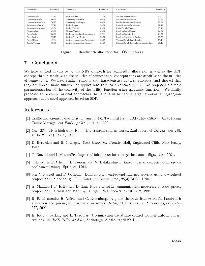
33.9380.0076.2727.1149.5443.6680.0033.1947.3455.06

London-ParisLondon-BrusselsLondon-AmsterdamAmsterdam-BerlinAmsterdam-BrusselsBrussels-ParisParis-BerlinParis-ZurichParis-MilanoZurich-Vienna

Connection Bandwith

Milano-Vienna-BerlinMilano-Paris-BrusselsBerlin-Amsterdam-BrusselsParis-Brussels-AmsterdamParis-Zurich-Vienna

37.0027.9322.0428.4225.48

London-Paris-MilanoLondon-Paris-ZurichLondon-Amsterdam-BerlinVienna-Zurich-Paris-LondonMilano-Zurich-Luxembourg-Amsterdam

24.7421.8723.7319.4628.42

71.5880.0080.0050.0063.0063.0027.1150.0035.7935.79

Connection Bandwith

Milano-ViennaBerlin-Amsterdam-LuxembourgZurich-Prague-BerlinZurich-Luxembourg-AmsterdamZurich-Luxembourg-Brussels

Zurich-MilanoCopenhaguen-BerlinCopenhaguen-PragueBerlin-PragueBerlin-Vienna

Connection Bandwith

Figure 11: Bandwidth allocation for COST network.

7 Conclusion

We have applied in this paper the NBS approach for bandwidth allocation, as well as the GPFconcept that is sensitive to the utilities of connections. concepts that are sensitive to the utilitiesof connections. We have studied some of the characteristics of these concepts, and showed thatthey are indeed more suitable for applications that have concave utility. We proposed a simpleparameterization of the concavity of the utility function using quadratic functions. We �nallyproposed some computational approaches that allows us to handle large networks: a Lagrangianapproach and a novel approach based on SDP.

References

[1] Tra�c management speci�cation, version 4.0. Technical Report AF-TM-0056.000, ATM ForumTra�c Management Working Group, April 1996.

[2] Cost 239. Ultra high capacity optical transmission networks, �nal report of Cost project 239.ISBN 953-184-013-X, 1999.

[3] D. Bertsekas and R. Gallager. Data Networks. Prentice-Hall, Englewood Cli�s, New Jersey,1987.

[4] T. Bonald and L.Massoulié. Impact of fairness on internet performance. Sigmetrics, 2001.

[5] S. Boyd, L. El Ghaoui, E. Feeron, and V. Balakrishnan. Linear matrix inequalities in systemand control theory. Springer, 1994.

[6] Jon Crowcroft and P. Oechslin. Di�erentiated end-to-end internet services using a weightedproportional fair sharing TCP. Computer Comm. Rev., 28(3):53�69, 1998.

[7] A. Maulloo F.P. Kelly and D. Tan. Rate control in communication networks: shadow prices,proportional fairness and stability. J. Oper. Res. Society, 49:237�252, 1998.

[8] R. R. Mazumdar H. Yaiche and C. Rosenberg. A game theoretic framework for bandwidthallocation and pricing in broadband networks. IEEE/ACM Trans. on Networking, 8(5):667�677, 2000.

[9] K. Kar, S. Sarkar, and L. Tassiulas. Optimization based rate control for multirate multicastsessions. In IEEE INFOCOM'01, Anchorage, Alaska, April 2001.

INRIA

[10] K. Kar, S. Sarkar, and L. Tassiulas. A simple rate control algorithm for maximizing total userutility. In IEEE INFOCOM'01, Anchorage, Alaska, April 2001.

[11] F. P. Kelly. Charging and rate control for elastic tra�c. European Trans. on Telecom., 8:33�37,1998.

[12] S. Kunniyur and R. Srikant. A time scale decompositon approach to adaptive � ECN marking.In IEEE INFOCOM'01, Anchorage, Alaska, April 2001.

[13] L.Massoulié and J. W. Roberts. Bandwidth sharing and admission control for elastic tra�c.Telecom. Systems, 2000.

[14] R. Mazumdar, L. G. Mason, and C. Douligeris. Fairness in network optimal �ow control:optimality of product forms. IEEE Trans. on Comm., 39:775�782, 1991.

[15] J. Mo and J. Walrand. Fair end-to-end window-based congestion control. In SPIE '98, Inter-national Symposium on Voice, Video and Data Communications, 1998.

[16] A. Nemirovski. What can be expressed via conic quadratic and semide�nite programming.Lecture notes, 1998.

[17] Scott Shenker. Fundammental design issues for the future internet. IEEE JSAC, 13(7):1176�1188, 1995.

RR n° 4269

Unité de recherche INRIA Sophia Antipolis2004, route des Lucioles - BP 93 - 06902 Sophia Antipolis Cedex (France)

Unité de recherche INRIA Lorraine : LORIA, Technopôle de Nancy-Brabois - Campus scientifique615, rue du Jardin Botanique - BP 101 - 54602 Villers-lès-Nancy Cedex (France)

Unité de recherche INRIA Rennes : IRISA, Campus universitaire de Beaulieu - 35042 Rennes Cedex (France)Unité de recherche INRIA Rhône-Alpes : 655, avenue de l’Europe - 38330 Montbonnot-St-Martin (France)

Unité de recherche INRIA Rocquencourt : Domaine de Voluceau - Rocquencourt - BP 105 - 78153 Le Chesnay Cedex (France)

ÉditeurINRIA - Domaine de Voluceau - Rocquencourt, BP 105 - 78153 Le Chesnay Cedex (France)

http://www.inria.fr

ISSN 0249-6399