Embed Size (px)
Citation preview

On Energy Efficient Routing Protocols
for
Wireless Sensor Networks
by
Suraj Sharma
Department of Computer Science and Engineering
National Institute of Technology Rourkela
Rourkela-769 008, Odisha, India
2016

On Energy Efficient Routing Protocols
for
Wireless Sensor Networks
Dissertation submitted in partial fulfillment of the requirements for the degree of
Doctor of Philosophy
in
Computer Science and Engineering
by
Suraj Sharma(Roll No: 509CS607)
under the guidance of
Prof. Sanjay Kumar Jena
Department of Computer Science and Engineering
National Institute of Technology Rourkela
Rourkela-769 008, Odisha, India
2016

Department of Computer Science and Engineering
National Institute of Technology Rourkela
Rourkela-769 008, Odisha, India.
Certificate
This is to certify that the work in the thesis entitled On Energy Efficient
Routing Protocols for Wireless Sensor Networks submitted by Suraj
Shrama is a record of an original research work carried out by him under my
supervision and guidance in partial fulfillment of the requirements for the award of
the degree of Doctor of Philosophy in Computer Science and Engineering. Neither
this thesis nor any part of it has been submitted for any degree or academic award
elsewhere.
Dr. Sanjay Kumar JenaProfessor
Date: Department of Computer Science & EngineeringPlace: NIT Rourkela National Institute of Technology
Rourkela-769008 Odisha (India)

Acknowledgements
My first thanks are to the Almighty God, without whose blessings I wouldn’t have
been writing this “acknowledgments”.
I then would like to express my heartfelt thanks to my guide, Prof. Sanjay
Kumar Jena, for his guidance, support, and encouragement during the course
of my Ph.D. at the National Institute of Technology, Rourkela. I am especially
indebted to him for teaching me both research and writing skills, which have been
proven beneficial for my current research and future career. Without his endless
efforts, knowledge, patience, and answers to my numerous questions, this research
would have never been possible. The experimental methods and results presented
in this thesis have been influenced by him in one way or the other. It has been a
great honor and pleasure for me to do research under Prof. Sanjay Kumar Jena’s
supervision.
I am very much indebted to Prof. S. K. Rath, Head of the Department,
Computer Science Engineering, National Institute of Technology, Rourkela for his
support during my work.
I am grateful to Prof. A. K. Turuk for teaching me the right way to present
the motivation for my thesis. His insightful feedback helped me improve the
presentation of the thesis in many ways. I am also thankful to Prof. Susmita Das,
Prof. B. Majhi, Prof. D. P. Mohapatra, Prof. Bibhudatta Sahoo, Prof. P. M.
Khilar, Prof. Pankaj Sa, Prof. K. Sathyababu for giving encouragement during
my thesis work.
I thank all the members of the Department of Computer Science and Engineering,
and the Institute, who helped me by providing the necessary resources, and in
various other ways, in the completion of my work.
Finally, I thank my parents and all my family member for their unlimited
support and strength. Without their dedication and dependability, I could not
have pursued my Ph.D. degree at the National Institute of Technology Rourkela.
Suraj Sharma
ii
Abstract
The sensor nodes communicate together by wireless techniques, and these
communication techniques are handled by routing protocols. The resource
limitation and unreliable low power links between the sensor nodes make it difficult
to design an efficient routing protocol. The sink may be either static or mobile
in the network. In many scenarios, static sink causes hotspots, where the sensor
nodes near to the sink die out soon due to transmission overhead. On the other
hand, the mobile sink improves the lifetime of a network by avoiding excessive
transmission overhead on the nodes that are close to the sink. Further, an attempt
is made to resolve the issues of sensor nodes and sink mobility by proposing
energy-efficient routing techniques for wireless sensor network.
A multipath routing protocol (MRP) is proposed, which reduces the control
overhead for route discovery and increases the throughput of the network. The
proposed multipath routing protocol is designed to improve the lifetime, latency
and reliability through discovering multiple paths from the source node to the
sink. MRP is a sink initiated route discovery process, where source node location
is known. In MRP, one primary path and number of alternate paths are discovered.
The sink may receive redundant data due to densely deployed sensor nodes.
Clustering the sensor nodes is an effective way to reduce the redundancy. The
cluster head aggregates the cluster members’ data before transmitting it to the
sink. A cluster based multipath routing protocol (CMRP) is proposed, where
the clustering technique reduces the data traffic in the network, and multipath
technique provides the reliable path.
Although, the hotspot problem can be resolved with mobile sink, it makes
the network dynamic. A tree-based data dissemination protocol with mobile sink
called TEDD is proposed to overcome the above problems. TEDD manages the
mobility of the sink and balances the load among the sensor nodes to maximize
the lifetime. A sensor node initiates the tree construction and becomes the root
node of the tree. Sensor nodes can send the data to the sink using this tree. It
iii

has been observed that the TEDD is a robust and energy-efficient protocol in the
mobile sink environment.
The proposed dense tree based routing protocol (DTRP) is an extension of
TEDD. The objectives of DTRP are to minimize the control overhead and reduce
the path length. Both the objectives are achieved by reducing the number of relay
nodes in the tree structure. DTRP resulted in, increased lifetime and reduced
end-to-end latency.
A clustered tree based routing protocol (CTRP) is designed to reduce the
data traffic in the network and efficiently manage the sink mobility. The traffic is
reduced by the cluster head, which uses the aggregation technique. The number
of cluster heads is restricted to the number of grids present in the network.
The CTRP efficiently manages the load among the sensor nodes. The tree is
constructed in the network using the cluster heads as vertices. The data can
be transmitted to the sink through the tree structure. The CTRP is compared
with the TEDD and DTRP in terms of energy efficiency, end-to-end latency, data
delivery ratio and network lifetime.
For the time-sensitive applications, a rendezvous based routing (RRP) with
mobile sink is designed. Each sensor node can communicate with the rendezvous
region. In RRP, two methods for data transmission are proposed. In the first
method, source node directly transmits their sensory data to the rendezvous area.
In the second method, the source node retrieves the sink’s current position and
sends the data to the sink through intermediate nodes. The end-to-end latency
and data delivery ratio are improved in the first proposed method. Whereas, the
energy consumption and lifetime in the second proposed method are enhanced.
iv

Contents
Certificate i
Acknowledgements ii
Abstract iii
List of Acronyms x
List of Notations xi
List of Figures xii
List of Tables xiv
List of Algorithms xv
1 Introduction 2
1.1 Routing in Wireless Sensor Network . . . . . . . . . . . . . . . . . . 3
1.2 Literature Review . . . . . . . . . . . . . . . . . . . . . . . . . . . . 4
1.2.1 Routing protocol with static sink . . . . . . . . . . . . . . . 4
1.2.2 Routing protocol with mobile sink . . . . . . . . . . . . . . . 16
1.3 Issues and Challenges for Routing in Wireless Sensor Networks . . . 22
1.3.1 Energy Management . . . . . . . . . . . . . . . . . . . . . . 24
1.3.2 Sink Mobility Management . . . . . . . . . . . . . . . . . . . 26
1.4 Motivation of the Research . . . . . . . . . . . . . . . . . . . . . . . 27
1.5 Objectives of the Research . . . . . . . . . . . . . . . . . . . . . . . 27
1.6 Organization of the Thesis . . . . . . . . . . . . . . . . . . . . . . . 28
2 Multipath Routing Protocol with Static Sink 32
2.1 Introduction . . . . . . . . . . . . . . . . . . . . . . . . . . . . . . . 32
2.2 System Model . . . . . . . . . . . . . . . . . . . . . . . . . . . . . . 33
v

2.2.1 Assumptions . . . . . . . . . . . . . . . . . . . . . . . . . . . 33
2.2.2 Network Model . . . . . . . . . . . . . . . . . . . . . . . . . 33
2.2.3 Energy Model . . . . . . . . . . . . . . . . . . . . . . . . . . 34
2.2.4 Performance Metrics . . . . . . . . . . . . . . . . . . . . . . 35
2.3 The Proposed Protocol . . . . . . . . . . . . . . . . . . . . . . . . . 36
2.3.1 Neighbor Discovery . . . . . . . . . . . . . . . . . . . . . . . 36
2.3.2 Multipath Construction . . . . . . . . . . . . . . . . . . . . 37
2.3.3 Data Transmission . . . . . . . . . . . . . . . . . . . . . . . 41
2.3.4 Rerouting and Route Maintenance . . . . . . . . . . . . . . 42
2.3.5 Energy Consumption Analysis . . . . . . . . . . . . . . . . . 43
2.4 Simulation Results . . . . . . . . . . . . . . . . . . . . . . . . . . . 45
2.4.1 Average Control Packet Overhead . . . . . . . . . . . . . . . 45
2.4.2 Average Energy Consumption . . . . . . . . . . . . . . . . . 46
2.4.3 Average End-to-End Latency . . . . . . . . . . . . . . . . . 47
2.4.4 Packet Delivery Ratio . . . . . . . . . . . . . . . . . . . . . 48
2.4.5 Network Lifetime . . . . . . . . . . . . . . . . . . . . . . . . 49
2.5 Summary . . . . . . . . . . . . . . . . . . . . . . . . . . . . . . . . 50
3 Cluster based Multipath Routing Protocol with Static Sink 52
3.1 Introduction . . . . . . . . . . . . . . . . . . . . . . . . . . . . . . . 52
3.2 System Model . . . . . . . . . . . . . . . . . . . . . . . . . . . . . . 53
3.2.1 Network Model . . . . . . . . . . . . . . . . . . . . . . . . . 53
3.2.2 Energy Model . . . . . . . . . . . . . . . . . . . . . . . . . . 53
3.3 The Proposed Protocol . . . . . . . . . . . . . . . . . . . . . . . . . 54
3.3.1 Neighbor Discovery and Topology Construction . . . . . . . 54
3.3.2 Cluster Head Selection and Cluster Formation . . . . . . . . 56
3.3.3 Data Transmission . . . . . . . . . . . . . . . . . . . . . . . 61
3.3.4 Re-clustering and Rerouting . . . . . . . . . . . . . . . . . . 62
3.4 Simulation Results . . . . . . . . . . . . . . . . . . . . . . . . . . . 62
3.4.1 Average Control Packet Overhead . . . . . . . . . . . . . . . 63
3.4.2 Average Energy Consumption . . . . . . . . . . . . . . . . . 64
vi

3.4.3 Average End-to-End Latency . . . . . . . . . . . . . . . . . 64
3.4.4 Packet Delivery Ratio . . . . . . . . . . . . . . . . . . . . . 65
3.4.5 Network Lifetime . . . . . . . . . . . . . . . . . . . . . . . . 66
3.5 Summary . . . . . . . . . . . . . . . . . . . . . . . . . . . . . . . . 67
4 Tree based Routing Protocol with Mobile Sink 69
4.1 Introduction . . . . . . . . . . . . . . . . . . . . . . . . . . . . . . . 69
4.2 System Model . . . . . . . . . . . . . . . . . . . . . . . . . . . . . . 70
4.2.1 Assumptions . . . . . . . . . . . . . . . . . . . . . . . . . . . 70
4.2.2 Network Model . . . . . . . . . . . . . . . . . . . . . . . . . 71
4.2.3 Mobility Model . . . . . . . . . . . . . . . . . . . . . . . . . 71
4.3 The Proposed Protocol . . . . . . . . . . . . . . . . . . . . . . . . . 72
4.3.1 Neighbor Discovery . . . . . . . . . . . . . . . . . . . . . . . 72
4.3.2 Tree Construction and Relay Node Selection . . . . . . . . . 74
4.3.3 Data Transmission . . . . . . . . . . . . . . . . . . . . . . . 76
4.4 Simulation Results . . . . . . . . . . . . . . . . . . . . . . . . . . . 77
4.4.1 Average Control Packet Overhead . . . . . . . . . . . . . . . 78
4.4.2 Average Energy Consumption . . . . . . . . . . . . . . . . . 79
4.4.3 Average End-to-End Latency . . . . . . . . . . . . . . . . . 80
4.4.4 Packet Delivery Ratio . . . . . . . . . . . . . . . . . . . . . 80
4.4.5 Network Lifetime . . . . . . . . . . . . . . . . . . . . . . . . 81
4.5 Summary . . . . . . . . . . . . . . . . . . . . . . . . . . . . . . . . 82
5 Dense Tree based Routing Protocol with Mobile Sink 84
5.1 Introduction . . . . . . . . . . . . . . . . . . . . . . . . . . . . . . . 84
5.2 System Model . . . . . . . . . . . . . . . . . . . . . . . . . . . . . . 85
5.2.1 Network, Energy, and Mobility Model . . . . . . . . . . . . . 85
5.3 Proposed Protocol . . . . . . . . . . . . . . . . . . . . . . . . . . . 85
5.3.1 Neighbor Discovery . . . . . . . . . . . . . . . . . . . . . . . 86
5.3.2 Tree Construction and Relay Node Selection . . . . . . . . . 87
5.3.3 Mobile Sink Management . . . . . . . . . . . . . . . . . . . 89
5.3.4 Data Transmission . . . . . . . . . . . . . . . . . . . . . . . 90
vii

5.3.5 Load Balancing and Tree Reconstruction . . . . . . . . . . . 92
5.4 Simulation Results . . . . . . . . . . . . . . . . . . . . . . . . . . . 95
5.4.1 Average Control Packet Overhead . . . . . . . . . . . . . . . 95
5.4.2 Average Energy Consumption . . . . . . . . . . . . . . . . . 96
5.4.3 Average End-to-End Latency . . . . . . . . . . . . . . . . . 97
5.4.4 Packet Delivery Ratio . . . . . . . . . . . . . . . . . . . . . 97
5.4.5 Network Lifetime . . . . . . . . . . . . . . . . . . . . . . . . 98
5.5 Summary . . . . . . . . . . . . . . . . . . . . . . . . . . . . . . . . 99
6 Clustered Tree based Routing Protocol with Mobile Sink 101
6.1 Introduction . . . . . . . . . . . . . . . . . . . . . . . . . . . . . . . 101
6.2 System Model . . . . . . . . . . . . . . . . . . . . . . . . . . . . . . 102
6.2.1 Network Model . . . . . . . . . . . . . . . . . . . . . . . . . 102
6.3 The Proposed Protocol . . . . . . . . . . . . . . . . . . . . . . . . . 102
6.3.1 Grid Construction . . . . . . . . . . . . . . . . . . . . . . . 103
6.3.2 Cluster Formation . . . . . . . . . . . . . . . . . . . . . . . 103
6.3.3 Tree Construction . . . . . . . . . . . . . . . . . . . . . . . . 105
6.3.4 Mobile Sink Management . . . . . . . . . . . . . . . . . . . 106
6.3.5 Data Transmission . . . . . . . . . . . . . . . . . . . . . . . 108
6.3.6 Load Balancing . . . . . . . . . . . . . . . . . . . . . . . . . 109
6.4 Simulation Results . . . . . . . . . . . . . . . . . . . . . . . . . . . 110
6.4.1 Average Control Packet Overhead . . . . . . . . . . . . . . . 110
6.4.2 Average Energy Consumption . . . . . . . . . . . . . . . . . 111
6.4.3 Average End-to-End Latency . . . . . . . . . . . . . . . . . 112
6.4.4 Packet Delivery Ratio . . . . . . . . . . . . . . . . . . . . . 113
6.4.5 Network Lifetime . . . . . . . . . . . . . . . . . . . . . . . . 113
6.5 Summary . . . . . . . . . . . . . . . . . . . . . . . . . . . . . . . . 114
7 Rendezvous based Routing Protocol with Mobile Sink 116
7.1 Introduction . . . . . . . . . . . . . . . . . . . . . . . . . . . . . . . 116
7.2 System Model . . . . . . . . . . . . . . . . . . . . . . . . . . . . . . 117
7.2.1 Network Model . . . . . . . . . . . . . . . . . . . . . . . . . 117
viii
7.3 The Proposed Protocol . . . . . . . . . . . . . . . . . . . . . . . . . 118
7.3.1 Neighbor Discovery . . . . . . . . . . . . . . . . . . . . . . . 118
7.3.2 Cross Area Formation . . . . . . . . . . . . . . . . . . . . . 119
7.3.3 Tree Construction . . . . . . . . . . . . . . . . . . . . . . . . 120
7.3.4 Sensor Node Region Discovery . . . . . . . . . . . . . . . . . 121
7.3.5 Data Transmission . . . . . . . . . . . . . . . . . . . . . . . 122
7.3.6 Proposed Method 1 . . . . . . . . . . . . . . . . . . . . . . . 123
7.3.7 Proposed Method 2 . . . . . . . . . . . . . . . . . . . . . . . 126
7.4 Simulation Results . . . . . . . . . . . . . . . . . . . . . . . . . . . 128
7.4.1 Average Control Packet Overhead . . . . . . . . . . . . . . . 129
7.4.2 Average Energy Consumption . . . . . . . . . . . . . . . . . 130
7.4.3 Average End-to-End Latency . . . . . . . . . . . . . . . . . 131
7.4.4 Packet Delivery Ratio . . . . . . . . . . . . . . . . . . . . . 132
7.4.5 Network Lifetime . . . . . . . . . . . . . . . . . . . . . . . . 132
7.5 Summary . . . . . . . . . . . . . . . . . . . . . . . . . . . . . . . . 133
8 Conclusions 135
8.1 Future Research Directions . . . . . . . . . . . . . . . . . . . . . . . 137
Bibliography 138
Dissemination 148
ix
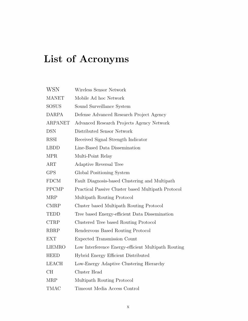
List of Acronyms
WSN Wireless Sensor Network
MANET Mobile Ad hoc Network
SOSUS Sound Surveillance System
DARPA Defense Advanced Research Project Agency
ARPANET Advanced Research Projects Agency Network
DSN Distributed Sensor Network
RSSI Received Signal Strength Indicator
LBDD Line-Based Data Dissemination
MPR Multi-Point Relay
ART Adaptive Reversal Tree
GPS Global Positioning System
FDCM Fault Diagnosis-based Clustering and Multipath
PPCMP Practical Passive Cluster based Multipath Protocol
MRP Multipath Routing Protocol
CMRP Cluster based Multipath Routing Protocol
TEDD Tree based Energy-efficient Data Dissemination
CTRP Clustered Tree based Routing Protocol
RBRP Rendezvous Based Routing Protocol
EXT Expected Transmission Count
LIEMRO Low Interference Energy-efficient Multipath Routing
HEED Hybrid Energy Efficient Distributed
LEACH Low-Energy Adaptive Clustering Hierarchy
CH Cluster Head
MRP Multipath Routing Protocol
TMAC Timeout Media Access Control
x

List of Notations
n Number of sensor nodes
V n Set of sensor nodes
(xi, yi) Location information of node i
d Distance in meter
d0 Threshold value of the distance
δ Pause time of the mobile sink
Sg Size of the grid
Gx grid coordinate of any node x
Er Residual energy of a sensor node
Ethreshold Threshold energy of a sensor node
ETX(k, d) Transmitting cost of k bits over d meters
ERX(k) Receiving cost of k bits
Eelec The energy consumption of amplifier to transmit or receive one bit
Eproc The processing cost of one-bit of data
εfs The energy cost of the amplifier to transmit one bit at one-hop
γ Path-loss-exponent
εmp The energy cost of the amplifier to transmit one bit at multi-hop
Elow The energy consumption of sensor node in sleep mode at one second
LF (i) Location factor of any node i
Nbr(i) One-hop neighbor set of any node i
idi Identity information of node i
NbrTable(i) One-hop neighbor information set of any node i
xi
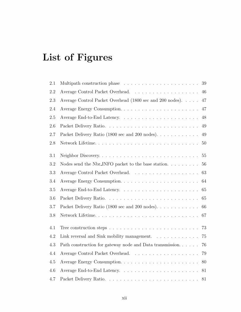
List of Figures
2.1 Multipath construction phase . . . . . . . . . . . . . . . . . . . . . 39
2.2 Average Control Packet Overhead. . . . . . . . . . . . . . . . . . . 46
2.3 Average Control Packet Overhead (1800 sec and 200 nodes). . . . . 47
2.4 Average Energy Consumption. . . . . . . . . . . . . . . . . . . . . . 47
2.5 Average End-to-End Latency. . . . . . . . . . . . . . . . . . . . . . 48
2.6 Packet Delivery Ratio. . . . . . . . . . . . . . . . . . . . . . . . . . 49
2.7 Packet Delivery Ratio (1800 sec and 200 nodes). . . . . . . . . . . . 49
2.8 Network Lifetime. . . . . . . . . . . . . . . . . . . . . . . . . . . . . 50
3.1 Neighbor Discovery. . . . . . . . . . . . . . . . . . . . . . . . . . . . 55
3.2 Nodes send the Nbr INFO packet to the base station. . . . . . . . . 56
3.3 Average Control Packet Overhead. . . . . . . . . . . . . . . . . . . 63
3.4 Average Energy Consumption. . . . . . . . . . . . . . . . . . . . . . 64
3.5 Average End-to-End Latency. . . . . . . . . . . . . . . . . . . . . . 65
3.6 Packet Delivery Ratio. . . . . . . . . . . . . . . . . . . . . . . . . . 65
3.7 Packet Delivery Ratio (1800 sec and 200 nodes). . . . . . . . . . . . 66
3.8 Network Lifetime. . . . . . . . . . . . . . . . . . . . . . . . . . . . . 67
4.1 Tree construction steps . . . . . . . . . . . . . . . . . . . . . . . . . 73
4.2 Link reversal and Sink mobility management. . . . . . . . . . . . . 75
4.3 Path construction for gateway node and Data transmission. . . . . . 76
4.4 Average Control Packet Overhead. . . . . . . . . . . . . . . . . . . 79
4.5 Average Energy Consumption. . . . . . . . . . . . . . . . . . . . . . 80
4.6 Average End-to-End Latency. . . . . . . . . . . . . . . . . . . . . . 81
4.7 Packet Delivery Ratio. . . . . . . . . . . . . . . . . . . . . . . . . . 81
xii

4.8 Network Lifetime. . . . . . . . . . . . . . . . . . . . . . . . . . . . . 82
5.1 Tree construction steps . . . . . . . . . . . . . . . . . . . . . . . . . 87
5.2 Gateway selection and Data transmission. . . . . . . . . . . . . . . 90
5.3 Control Packet Overhead. . . . . . . . . . . . . . . . . . . . . . . . 96
5.4 Average Energy Consumption. . . . . . . . . . . . . . . . . . . . . . 96
5.5 Average End-to-End Latency. . . . . . . . . . . . . . . . . . . . . . 97
5.6 Packet Delivery Ratio. . . . . . . . . . . . . . . . . . . . . . . . . . 98
5.7 Network Lifetime. . . . . . . . . . . . . . . . . . . . . . . . . . . . . 98
6.1 Grid Construction. . . . . . . . . . . . . . . . . . . . . . . . . . . . 104
6.2 Cluster Head selection and Cluster formation. . . . . . . . . . . . . 104
6.3 Tree Construction and Mobile Sink Management. . . . . . . . . . . 107
6.4 Control Packet Overhead . . . . . . . . . . . . . . . . . . . . . . . . 111
6.5 Average Energy Consumption . . . . . . . . . . . . . . . . . . . . . 111
6.6 Average End-to-End Latency . . . . . . . . . . . . . . . . . . . . . 112
6.7 Packet Delivery Ratio . . . . . . . . . . . . . . . . . . . . . . . . . . 112
6.8 Network Lifetime . . . . . . . . . . . . . . . . . . . . . . . . . . . . 113
7.1 Rendezvous region and Backbone nodes. . . . . . . . . . . . . . . . 119
7.2 Rendezvous region and Tree within the rendezvous region. . . . . . 121
7.3 Sensor node region discovery and Gateway node selection. . . . . . 122
7.4 Data transmission using Proposed Method 1. . . . . . . . . . . . . . 124
7.5 Data transmission using Proposed Method 2. . . . . . . . . . . . . . 126
7.6 Control Packet Overhead. . . . . . . . . . . . . . . . . . . . . . . . 130
7.7 Average Energy Consumption. . . . . . . . . . . . . . . . . . . . . . 130
7.8 Average End-to-End Latency. . . . . . . . . . . . . . . . . . . . . . 131
7.9 Packet Delivery Ratio . . . . . . . . . . . . . . . . . . . . . . . . . . 132
7.10 Network Lifetime . . . . . . . . . . . . . . . . . . . . . . . . . . . . 133
xiii

List of Tables
2.1 Simulation Parameters. . . . . . . . . . . . . . . . . . . . . . . . . . 45
3.1 Neighbor Adjacency Matrix. . . . . . . . . . . . . . . . . . . . . . . 56
3.2 Simulation Parameters . . . . . . . . . . . . . . . . . . . . . . . . . 63
4.1 Simulation Parameters. . . . . . . . . . . . . . . . . . . . . . . . . . 78
5.1 Simulation Parameters. . . . . . . . . . . . . . . . . . . . . . . . . . 95
6.1 Simulation Parameters. . . . . . . . . . . . . . . . . . . . . . . . . . 110
7.1 Simulation Parameters. . . . . . . . . . . . . . . . . . . . . . . . . . 129
xiv

List of Algorithms
2.1 Neighbor Discovery . . . . . . . . . . . . . . . . . . . . . . . . . . . 37
2.2 Multipath Construction . . . . . . . . . . . . . . . . . . . . . . . . 40
3.1 Neighbor Discovery and Topology Construction . . . . . . . . . . . 55
3.2 Cluster Head Intimation . . . . . . . . . . . . . . . . . . . . . . . . 59
3.3 Cluster Formation . . . . . . . . . . . . . . . . . . . . . . . . . . . . 60
4.1 Neighbor Discovery . . . . . . . . . . . . . . . . . . . . . . . . . . . 73
4.2 Tree Construction and Relay node Selection . . . . . . . . . . . . . 74
4.3 Data Transmission . . . . . . . . . . . . . . . . . . . . . . . . . . . 77
5.1 Neighbor Discovery . . . . . . . . . . . . . . . . . . . . . . . . . . . 86
5.2 Tree Construction and Relay Node Selection . . . . . . . . . . . . . 88
5.3 Mobile Sink Management . . . . . . . . . . . . . . . . . . . . . . . . 91
5.4 Data Transmission . . . . . . . . . . . . . . . . . . . . . . . . . . . 92
5.5 Load Balancing and Tree Reconstruction . . . . . . . . . . . . . . . 93
6.1 Cluster Formation . . . . . . . . . . . . . . . . . . . . . . . . . . . . 105
6.2 Tree Construction . . . . . . . . . . . . . . . . . . . . . . . . . . . . 106
6.3 Mobile Sink Management . . . . . . . . . . . . . . . . . . . . . . . . 108
6.4 Data Transmission . . . . . . . . . . . . . . . . . . . . . . . . . . . 109
7.1 Neighbor Discovery . . . . . . . . . . . . . . . . . . . . . . . . . . . 119
7.2 Node Region Discovery . . . . . . . . . . . . . . . . . . . . . . . . . 123
7.3 Mobile Sink Management (Proposed Method 1) . . . . . . . . . . . 125
7.4 Mobile Sink Management (Proposed Method 2) . . . . . . . . . . . 127
7.5 Sink Location Recovery (Proposed Method 2) . . . . . . . . . . . . 128
xv

Introduction
Routing in WSN
Literature Review
Issues and Challenges for Routing in WSN
Motivation of the Research
Objectives of the Research
Organization of the Thesis

Chapter 1
Introduction
Nowadays, the research in Wireless Sensor Network (WSN) is growing due
to the advancement of embedded system and wireless technology [1]. WSN has
numerous applications in our environment, community, locality, workplace, home
and beyond [2]. It is providing new origins of ideas, comfort and ease in the
personal and professional life.
The development of WSN started in the 1950s when US military developed the
Sound Surveillance System (SOSUS) used in submerged acoustic sensors [3]. For
seismic activity surveillance, some of the sensors of SOSUS are still in use. After
a gap of nearly three decades the Defense Advanced Research Project Agency
(DARPA) in USA started the Distributed Sensor Network (DSN) program that
focused on further developments on newly invented technologies and protocols in
context of their use for sensor networks [4]. Simultaneously, Advanced Research
Projects Agency Network (ARPANET) started research and development in
the WSN by involving many institutions and industries [5]. The research and
development on small sensor nodes were initiated by NASA ‘Sensor web project’
and ‘Smart dust project’ in the year 1998 [6]. One of the objectives of the above
project was to create autonomous sensing and communication device within a
cubic millimeter of space. Other early projects in this area started around 1999 was
primarily in academia at several places, including MIT, Berkeley and University
of Southern California [7].
Wireless Sensor Network contains hundreds of thousands of low-cost sensor
nodes. A sensor node has constraints like storage, energy, limited processing
2

Chapter 1 Introduction
and transmitting capability [8]. The sensor node monitors the physical and
environmental condition, such as temperature, pressure, motion, fire, humidity and
many more. WSN is applicable for tracking, surveillance, monitoring, healthcare,
disaster relief, event detection, biodiversity mapping, intelligent building, facility
management, preventive maintenance, etc. Generally, sensor nodes are deployed
in an unattended and hostile environment for monitoring wild forest, battlefield,
chemical plants, nuclear reactors and so on [9]. So it becomes a strenuous
task to replace or recharge the battery. The sensor node senses not only the
environment but also forwards the data to the base station (sink). A base station
is a resource-rich device having unlimited power, communication and storage
capability. It may be a static node or a mobile node based on the applications
and scenarios. It can communicate with the sensor nodes, to collect the data
and sends to the user via existing communication system or the Internet. The
research have conducted on the data collection among sensors, processing and
routing the data during recent years [10–17]. As the sensor network operates in
an energy constraint environment, the network often requires an energy-efficient
routing protocol to enhance the lifetime of the network.
1.1 Routing in Wireless Sensor Network
Routing technique plays a vital role in the wireless sensor network. It is
extremely difficult to assign the global ids for a large umber of deployed sensor
nodes. Thus, traditional protocols may not be applicable for WSN. Unlike
conventional wireless communication networks (MANET, cellular network, etc.),
WSN has inherent characteristics. It is highly dynamic network and specific to
the application, and additionally it has limited energy, storage, and processing
capability. These characteristics make it a very challenging task to develop a
routing protocol [18–20]. In most of the scenarios, multiple sources are required
to send their data to a particular base station. The nodes near to the sink, depleted
more energy and hence eventually die. This causes partitioning of the network;
consequently, the lifetime of the network gets to reduce. The main constraint of the
3

Chapter 1 Introduction
sensor node is energy [21,22]. The sensors are battery-powered computing devices.
It’s hard to replace the batteries in many applications. Therefore, WSN requires
an energy-efficient routing protocol. Due to dense deployment, the sensor nodes
generate the redundant data, and the base station may receive multiple copies
of the same data. Therefore, it unnecessarily consumes the energy of the sensor
nodes. WSN does not have any fixed infrastructure and is highly dynamic [23].
There are mainly two reasons responsible for the dynamic infrastructure. The first
reason is the energy; the sensor nodes have limited energy in the form of batteries.
If the protocol is unable to balance the load among the nodes, the sensor node
could die. It leads to the dynamic network structure. The second reason is the
mobility; in many scenarios after the deployment, sensor nodes are static but sink
can move within the network. It makes the network dynamic, and the protocol
that works for static sink may not be applicable for mobile sink [24]. In many
applications, sensor nodes are required to know their location information. It is
not feasible to enable all nodes with Global Positioning System (GPS) [25]. So the
protocol should have to take the help of the techniques like triangulation based
positioning [26], GPS-free solutions [27], etc. to get the approximate location
information.
1.2 Literature Review
Various researchers have contributed in the area of the routing protocol in
wireless sensor networks. Technique reported for routing protocol may be broadly
categorized into two groups:
1. Routing protocol with static sink.
2. Routing protocol with mobile sink.
1.2.1 Routing protocol with static sink
The routing protocol with static sink can be classified into hierarchical-based,
multipath-based, location-based and hybrid routing. In the hierarchical structure,
the network nodes are divided into two categories; one work for data collection
4

Chapter 1 Introduction
and sending it to the base station and other sense the environment. The objective
of the multipath routing is to provide reliability to the network through available
paths between a sensor and the sink. In the location based routing sink knows the
location of the source node. Sink sends the query to an interested location to get
the data. The combination of two or more above routing protocols can be known
as the hybrid routing protocol.
• Hierarchical-based Routing In the hierarchical architecture, some
higher-energy nodes can be used to process and send the information to the
base station while lower energy nodes can perform the sensing in the target
area. In other words, the network is partitioned into many clusters. In each
cluster, a node is selected as a cluster head with some cluster members. A
two-tier hierarchy is formed where cluster heads are in the higher tier while
cluster members are created a lower tier. Cluster members sense the data
from the physical environment and send it to their respective cluster heads.
Cluster heads process the data and transmit it to the sink either directly or
in the multi-hop manner.
Low-Energy Adaptive Clustering Hierarchy (LEACH) protocol has been
proposed by Heinzelman et al. [28]. It is the first hierarchical clustering
approach in WSN. In the LEACH protocol, the operation consists of many
rounds. Each round has two phases; the set-up phase and steady-state phase.
In the setup phase, the cluster is formed and in the steady-state phase, data
is transmitted to the base station. The cluster head are elected based on
the predefined percentage of cluster heads and how many times the node has
been a cluster head in previous rounds. LEACH can balance the load among
the cluster heads up to some extent. Individual time slot prevents cluster
head from unnecessary collisions and avoids excessive energy dissipation. On
the contrary, LEACH is not applicable to large-area networks, and uneven
distribution of cluster head brings extra overhead.
Younis and Fahmy have proposed a Hybrid Energy Efficient Distributed
clustering (HEED) routing protocol [29]. It is a multi-hop clustering
5
Chapter 1 Introduction
algorithm for wireless sensor networks, which focus on efficient clustering
by proper selection of cluster heads. The cluster head is selected based
on criteria such as residual energy and intra-cluster communication cost.
HEED is a fully distributed clustering method and provides uniform CH
distribution across the network. The communications are in a multi-hop
fashion between CHs and the base station. However, it generates more CHs
than the expected number, which decreases the network lifetime.
Power efficient gathering in sensor information systems has been proposed
by Lindsey et al. [30]. It is an improvement over LEACH protocol. This
protocol requires the formation of a chain that is achieved in two steps: chain
construction and gathering data. The basic idea of the protocol is that the
nodes need to transmit only with their closest neighbors, and they take turns
in communicating with the base station. It reduces the overhead of dynamic
formation of clusters, and through the chain method, it decreases the data
transmission. The energy load is dispersed uniformly in the network. In
contrast, the delay is increased for the distant nodes due to a single chain
and can reduce the performance.
Huan Li et al. [31] have proposed an approach for constructing optimal
clustering architecture. The node with high residual energy claims as the
new cluster head. Then the cluster head collects all the data from their
neighboring nodes and sends it to the sink. It selects the cluster head who
has highest residual energy. It obtained an optimum number of clusters to
cover a sensing area to minimize the energy consumption per cluster. Also
the variance of energy consumption among the clusters. Although it is a
distributed protocol and works well with a large number of sensor nodes, it
consumes a large amount of energy in obtaining residual energy information
of the neighbor nodes.
Ouadoudi Zytoune et al. [32] have proposed an energy aware clustering
technique, where the network is divided into clusters. A cluster head is
selected to monitor and control the cluster. The cluster head can directly
6

Chapter 1 Introduction
transmit the data to the base station. The cluster heads are elected based
on the ratio of residual energy and the average energy of the network.
This protocol provides a stable network. It reduces the number of control
message, so the lifetime increases. On the other hand, it is only suitable for
heterogeneous network and work for limited applications.
A clustering technique called the limiting member node clustering proposed
by W. Naruephiphat et al. [33]. This algorithm considers a maximum
number of member nodes for each cluster head. It divides sensor nodes
into groups where nodes within the transmission range of base station are
defined in level 1 and nodes far from the base station are defined in a higher
levels depending on the distance from the base station. In this approach,
each sensor node selects a cluster head from the candidate list of cluster
heads based on a cost function that considers energy consumption, battery
level and distance from the base station. This protocol will limit the number
of member nodes of each cluster head to be less than a threshold value in
order to distribute the burden of each cluster head. It prolongs the network
lifetime and reduces the time to forward the data packet to the base station.
Chang and Ju [34] have proposed a save energy clustering algorithm. In this
algorithm, the cluster head election process includes location, the average
residual energy of the sensor nodes and residual energy for each sensor
node. The sensor node becomes a candidate cluster head when the residual
energy of the node is greater than the average residual energy of the sensor
nodes. The load balancing among the clusters can prolong the lifetime of the
network. It consumes low energy that extend the network lifetime. However,
it is a centralized algorithm and required the location information of each
node.
A centralized energy-efficient routing protocol called LEACH-C has been
proposed by Muruganthan et al. [35]. LEACH-C is a modified LEACH using
centralized clustering control. In the setup phase, the base station collects
the location information and residual energy of each node in the network and
7

Chapter 1 Introduction
based on this base station selects the cluster heads and configures the rest of
the nodes into clusters. Both intra-cluster communication and inter-cluster
communication are single-hop communication. Since the base station has the
knowledge of the network and information of energy and location of sensor
nodes, it creates better clusters that require less energy for transmitting
data. In contrast, it causes extra overhead on providing the information to
the base station and is not applicable for large networks.
• Multipath-based Routing Multipath routing is an alternative routing
technique, which selects multiple paths to deliver data from source to
destination. It allows multiple paths between the source and the sink. Due
to the use of redundant paths, multipath routing can largely address the
reliability and load balancing issues. Many multipath routing protocols have
been proposed for WSNs. The existing protocols on multipath routing tried
to cope with load balancing and resource limitations of the low-power sensor
nodes through concurrent data forwarding over multiple paths.
Directed Diffusion routing protocol has been proposed by Intanagonwiwat
et al. [36]. It is a query based multipath routing protocol, where the
sink initializes the routing process. The sink floods the interest into the
network. During the interest message flooding all the intermediate nodes
store the interest message received from the neighbors for later use and
creates a gradient towards the sender node. During this stage, multiple
paths can be discovered between each source-sink pair. Then the source
transmits the data through the selected path. Further the sink continues
to send low-rate interest message over the remaining paths, this is done
to preserve the freshness of the interest tables of the intermediate nodes,
and also maintain the discovered routes. If the active path fails, the data
can be forwarded through the other available paths. Although, it provides
fault-tolerant routing, it evolves all the nodes in route discovery. As a result,
it affects the network lifetime.
Ganesan et al. [37] have proposed a braided multipath routing protocol,
8

Chapter 1 Introduction
which constructs multiple partially disjoint paths. It provides fault
tolerance in the sensor network. This protocol establishes routes using
two path reinforcement messages. One is the primary path, and another
is the alternate path reinforcement message. The sink initializes the path
construction by sending a primary path reinforcement message to the best
next-hop neighbor towards the source node. This process continues until
the primary reinforcement message reaches the source node. The primary
node also sends the alternative path reinforcement message to the next-best
neighbor towards the node of origin.
This process results in the construction of backup paths. Whenever the
primary path fails, data can be forwarded through the alternate path.
Ye Ming Lu et al. [38] have proposed a distributed, scalable and localized
routing algorithm . It discovers multiple node-disjoint paths between the
sink and the source nodes. It also uses a load balancing algorithm that
distributes the traffic over the multiple paths. When an event is detected, it
selects a node from the event area as the source node. The source node
then starts the route discovery process. The sink sends multiple route
request messages to its neighboring nodes with distinct path id to build
node-disjoint paths. After receiving the first route request message from the
source node, the sink starts a timer. Any path discovered after the timer
stops are discarded. The sink also optimally assigns the data rate for each
path.
M. Maimour [39] has proposed a Maximally Radio-disjoint multipath routing
(MR2), which deals with the interfering paths. Its main objective is to
provide the necessary bandwidth to multimedia data through non-interfering
paths. It constructs the minimum interfering paths using the adaptive
incremental method. Only one path is built at a time, and additional paths
are constructed when required, typically in case of network congestion or
bandwidth shortage. The protocol reduces the effects of interference by
keeping some sensor nodes in the sleep state. After going to sleep state,
9

Chapter 1 Introduction
the sensors will not take part in any routing process. However, MR2 is
only suited for the query based applications and used flooding technique to
construct non-interfering paths.
Wang et al. [40] have proposed an energy-efficient and collision-aware
multipath routing protocol. It is a reactive routing protocol. It creates
two collision-free paths between the source and the sink using the location
information of all the sensor nodes. In this protocol, each node sends a route
discovery message with proper power and node position information. It is
assumed that all nodes have a transmission range of 0 to R, and all nodes
know their neighbor information within that range R. Hence to decrease
the chance of interference, all routing paths are built above this range. The
broadcasting is used to detect collision, and the nodes that are overhearing
from other routes cannot be in any route. However, the cost of the network
deployment is more due to the GPS device requirements for each node within
the network.
Low Interference Energy-efficient Multipath ROuting (LIEMRO) has been
proposed by Radi et al. [41]. It improves the latency, lifetime and packet
delivery ratio by applying node-disjoint paths. It includes a load balancing
algorithm to distribute the source node traffic over multiple paths based
on the relative quality of each path. It also calculates the cost of the link,
which is done by the Expected Transmission Count (ETX) [42] metric. In
this method, the sink sets its cost to zero and broadcast a control packet to
its neighbors. Each neighbor then calculates its link cost with respect to the
sink. Further, they broadcast the information in the network until the source
node receives the information. The route discovery phase is initialized, as
soon as an event is detected in the network. The source sends the route
request to the sink to start the route establishment. The path with lesser
residual energy transmits the data with a lower rate to save the energy.
LIEMRO maintains the traffic rate dynamically based on the quality of the
paths. However, it does not consider the service rate and the buffer capacity
10

Chapter 1 Introduction
of the active nodes to adjust and predict the traffic rate of the active paths.
Cherian et al. [43] presents a novel multipath routing algorithm that
increases the reliability by using multiple paths and scheduling data
transmission rates at each node. This approach helps to prevent congestion
and packet loss. Each node in the network maintains two queues for incoming
data and three queues for transmitting the data. Also, every packet is
assigned a priority number based on its information. All the nodes in the
network act as a scheduling unit and whenever any node receives the data
packet, they put the packet in the appropriate queue. Later on, the node will
select the packet based on the priority number from the queue and schedule
a transmission to its next available multiple nodes. By using this approach
the traffic on the network, is controlled by adjusting the queue length. It
provides a high rate of reliability in the presence of channel errors. However,
it does not provide a way to detect the failed nodes.
• Location-based Routing In the location-based routing, sensor nodes are
known by their locations. The node can find the distance to the neighbor
based on the received signal strength. The relative coordinates location
information can be calculated by exchanging the control packets between the
neighbor nodes. Alternatively, each node has to use the Global Positioning
System (GPS) [25]. The unknown nodes can calculate approximate location
information by referring the position of the known nodes.
Greedy perimeter stateless routing has been proposed by Karp and Kung
[44]. It makes the data packet forwarding decisions using nodes location
information. It uses greedy forwarding and perimeter forwarding techniques
to forward data packets to the nodes that are always closer to the target
node. In regions of the network where such a greedy path does not exist,
the protocol recovers by forwarding in perimeter mode. The position
of a packet’s destination and positions of the next hop neighbor are
sufficient to make correct forwarding decisions, without any other topological
information.
11

Chapter 1 Introduction
Y. Xu et al. [45] have proposed a geographic adaptive fidelity routing. In this
approach, the network is partitioned into equal sized virtual grids. Inside
each grid, nodes will elect one sensor node as a leader to stay awake for some
duration and other nodes can switch to sleep mode. This node monitors and
reports the event to the base station on behalf of the other nodes in the grid.
Thus, the network conserves energy without affecting the routing accuracy.
Each node has three defined states: discovery, active and sleep. However, the
leader node does not do perform any aggregation as hierarchical protocols
discussed earlier.
Zhang et al. [46] have proposed an Energy-efficient geographic routing.
It considers both nodes location information and energy consumption for
making routing decisions. Instead of forwarding the data packets to the
neighbor closest to the sink or neighbor has maximum residual energy, the
packet are transmitted to the neighbor that is closer to the energy optimal
relay position. In this protocol, all nodes are not required to maintain
neighbor information. The optimal relay node is computed by broadcasting
small control packets having the location and residual energy information.
It is fully localized, stateless and energy-efficient protocol. It only works well
in the uniformly deployed network.
Alasem et al. [47] have proposed location-based energy aware and reliable
routing, which is based on sensor position. The location information that
has been used in the protocol could be extracted from GPS. Each node
sends its location information to its neighbors and constructs a routing table.
The routing table consists of neighbor node id and the distance from the
destination node. The routing decision is taken by the source using the
distance. The node with the shortest distance is selected as the candidate
relay node to send the information.
A reactive geographic routing protocol has been proposed by Ding et al.
[48]. It combines reactive routing mechanism and geographic routing. It
is calculating the shortest distance between destination node and neighbor
12

Chapter 1 Introduction
node. The protocol uses two new measures to improve the performance of
routing protocol. First, to reduce the consumption, it uses reactive routing
mechanism to mitigate the routing overhead. Second, to improve reliability,
it finds the optimal path from the many available paths.
Energy-efficient geographic routing algorithm has been proposed by Chen et
al. [49]. It considers three factors for the routing decision such as routing
distance, signal interference, and computation cost. In the protocol, two
methods for the routing decision have been proposed. In the first method,
it takes the decision based on the distance and signal interference. It finds
the Euclidean distance from the transmitter node to the destination node
and interference power. In the second method, it takes the decision based
on the maximum power consumption and interference power.
• Hybrid Routing The hybrid routing is a combination of any of the above
routing protocols. It takes the benefits of more than one protocols to enhance
the performance of the network. Many researches have been done using the
hybrid approach in the routing protocol for wireless sensor network.
Bagheri et al. [50] have proposed reliable and energy efficient clustering based
multipath routing protocol, where nodes are enabled with the GPS. The
cluster head section is based on the remaining energy of the node. The sink
initiated the route discovery by sending a request packet to its nearby cluster
heads, and request reaches the source cluster head. The source cluster head
may receives more than one requests. The multipath routes are constructed
through the cluster heads. A cluster head selects another path if existing
path fails.
An event-based multipath clustering protocol has been proposed by Quynh et
al. [51]. When an event is detected, all nodes near the event will active. One
of the nodes close to the event having maximum residual energy is elected
itself as the cluster head. The rest of the active nodes join the cluster head
and form the cluster. The cluster head chooses the relay node and backup
relay node towards the sink to form the multipath. When the link fails, the
13

Chapter 1 Introduction
protocol selects the backup relay node for data transmission.
Mazaheri et al. [52] have proposed a QoS base energy aware multipath
hierarchical routing. It elects the cluster head in the range r based on
the remaining energy and the distance from the sink. For multipath
construction, cluster head chooses a set of cluster heads within the range
R (where, R > r) based on the residual energy, remaining buffer size, signal
to noise ratio and distance to the sink. It distributes the load among the
relay paths to send the data, which reduces the end-to-end latency.
A Practical Passive Cluster based Multipath Protocol (PPCMP) has been
proposed by Jin et al. [53]. In this protocol, the node near to the event
becomes the candidate cluster head and waits for a certain time. If it does
not receive any cluster head advertisement within that time, it becomes the
cluster head and broadcasts the advertisement in its range (R). The node
resides within R2
range joins the cluster and rest of the nodes up to the
range R become the candidate cluster head and follow the same procedure
for cluster formation. Branch aware flooding method [54] is used to construct
the multipath between the sink and the source node. For the next time if
any source detected the event, the same available set of clusters are used,
but a new set of multipath is required for data transmission. In the protocols
[50–53] the control packet overhead is more, which leads to the higher energy
consumption. It directly affects the lifetime of the network. These protocols
give more emphasis on reliability through the multipath but neglect some
QoS parameters such as end-to-end delay, control overhead and network
lifetime.
A cross-layer based clustered multipath routing has been proposed by
Almalkawi et al. [55]. The nodes are heterogeneous and randomly deployed.
The sink initiated the cluster formation by broadcasting the control packet.
Based on the received signal strength the powerful nodes become the cluster
heads. The cluster heads are classified in different levels. They send the
data through the upper-level cluster head.
14

Chapter 1 Introduction
A Fault Diagnosis based Clustering and Multipath routing (FDCM) has
been proposed by W. Liu [15]. For cluster formation, base station randomly
chooses a particular number of candidate cluster heads on certain probability.
The candidate cluster head checks the fault status of each other. Once the
faulty node is detected, it is removed from the network. Among the neighbor
candidate cluster head having the highest residual energy becomes the cluster
head and the non-cluster head nodes join the closest cluster head and form
the cluster. For multipath construction, a cluster head chooses the cluster
head within the 2R range having the smallest distance from the sink. The
protocols [15, 55, 56] do not maintain the proper path. They only have the
information regarding neighbor nodes. They have to choose a node from the
neighbor list without knowing their current residual energy or connectivity
with the other nodes. It decreases the reliability of the networks.
Wang et al. [57] have proposed a hierarchical multipath routing protocol.
Each node has a hop count value that indicates the distance to the sink.
Based on the hop count the node selects the parent and alternate parent
node to make the multipath. The network looks like a tree with the sink as
the root node. Using hierarchical structure, it reduces some amount of data
traffic and energy consumption.
Yang et al. [58] have proposed an event based routing protocol. The node
closest to the event becomes the cluster head and the node that satisfies
certain threshold joins the cluster head. The ant colony algorithm [59] was
used to create multipath between the cluster head and the sink. The cluster
head dynamically chooses the routing path between the available path to
send the aggregated data to the sink. The protocols [15, 52, 55, 57, 58] have
not used any load balancing technique among the nodes. It leads to the
mismanagement of the network and reduces the throughput and network
lifetime.
15

Chapter 1 Introduction
1.2.2 Routing protocol with mobile sink
In the routing protocol with static sink, the sensor nodes close the sink always
forward a large amount of data; as a result they die. Finally, the network is
partitioned, and the sink can not receive any data. This phenomena is known
as crowded center effect [60] or energy hole problem [61]. A mobile sink is used
in the network to overcome this problem. The mobile sink makes the network
dynamic, and routing becomes difficult. In this section, a study on the existing
routing protocols with mobile sink is done. They are categorized and explained.
The routing protocol with mobile sink can be classified into hierarchical-based,
tree-based and virtual-structure-based.
• Hierarchical-based Routing In hierarchical routing protocols, the entire
network is broken into layers. The higher layer nodes are assigned some
specific tasks like processing and sending the information while the lower
layer nodes are used for sensing in the proximity of the target. Data travels
from the lower layer nodes to the higher layer nodes while the queries go
from, the higher layer nodes to the lower layer nodes. In the hierarchical
approach, a virtual hierarchy of nodes is created in the network that imposes
different dynamic roles on the sensors. The hierarchy might be composed
of two or more tiers. A successful hierarchical approach must employ easily
accessible structure and should avoid energy hole problem [61] on the higher
tier nodes.
Lin et al. [62] have proposed a hierarchical cluster-based data dissemination
protocol. It uses a clustering structure to track the location of the mobile
sinks and finds the paths from the source to the sink for data transmission.
Each cluster consists of a cluster head, several gateway nodes, and ordinary
nodes. The mobile sink registers itself to the nearest cluster head, and a
notification is then disseminated to all the cluster heads. In this process,
each cluster head makes a reverse link to the sender node for transmitting
the data.
A mobile routing algorithm in cluster-based architecture has been proposed
16

Chapter 1 Introduction
by Wang et al. [63]. Each sensor node finds the neighbor information like
its residual energy and location by broadcasting a small control packet. The
cluster heads are elected based on the higher residual energy among the
neighbors. The cluster head broadcasts the advertisement to create a cluster.
The cluster members join the cluster head and form a cluster. The mobile
sink moves within the network using the random waypoint mobility model.
The sink broadcasts the location information when it reaches to the new
location. The cluster heads create the routing path based on the location
information and send the aggregated data to the sink.
A mobile-sink based energy-efficient clustering algorithm has been proposed
by Wang Yin et al. [64]. In this approach, the cluster head is selected based
on the residual energy. The cluster head aggregates the data and transmits
it to the mobile sink. The mobile sink sends their location information just
for once. The sink follows the paths that are easily predictable by the sensor
nodes. The sensor nodes keep track of the current position of the sink by
calculating it using the initial location of the sink. However, this protocol
performs well in the predictable mobility model environment.
Wang et al. [65] have proposed an energy-aware data aggregation scheme. It
is a hierarchical hybrid routing protocol that comprises of on-demand data
dissemination tree with grid structure. Sensor nodes enabled with Global
Positioning System (GPS). A gateway node is selected with highest residual
energy around the sink. Gateway node is responsible for aggregating data,
forwarding the sink queries towards the interest zone and transferring the
source generated data to sink. It is changed periodically according to sink
movement. Energy consumption of this protocol is less when maximum sink
speed is considered. It performs in-route data aggregation, which increase
the energy efficiency.
• Tree-based Routing The management of sink mobility is very importance
in the mobile sink environment. The tree-based routing is the efficient
solution to that problem. Through the connected structure like a tree, it
17

Chapter 1 Introduction
is very easy to manage the sink mobility. In the tree structure, any source
node can send their data to the sink with minimal cost.
Kim et al. [66] have proposed scalable energy-efficient asynchronous
dissemination protocol. It constructs a tree to disseminate the data to the
sink through an access node. It is the sensor node that send the data directly
to the sink and location of the sink known to the access node. Sink elects
an access node when it reaches a new location. The dissemination tree is
reconstructed in the case where the sink elects the new access node. In
this protocol, a trade-off exists between minimizing the delay and saving the
energy spent on reconfiguring the tree. The sink can move without reporting
their location to the tree. The concept of the access node is well defined for
the real-time applications. However, The tree construction is required when
sink elects the new access node, which increases the overall cost.
Adaptive Reversal Tree (ART) protocol has been proposed by Hwang et
al. [67]. Here, a tree with a temporary root is constructed, and all paths are
directed toward the root. The root node is linked with the sink. The source
node sends their data to the sink through this tree. The sink selects a new
neighbor node as the root node. The new root node reconfigures the affected
area. The tree structure changes based on the new position of the sink. The
efficiency path-repair method reduces the communication overhead, but the
routing paths are sub-optimal, which increases the latency.
Wang et al. [68] have proposed a local update-based routing protocol. The
basic idea behind this protocol is to restrict the scope of the frequent location
updates for a mobile sink to a local area called a destination area, and hence
reduce communication overhead. In this protocol, a mobile sink defines a
circular destination area by selecting its current position as a virtual center
and an updated range of L. The location of the virtual center and the
selected update range are then flooded across the entire network. When the
mobile sink moves inside its destination area, it only broadcasts the location
information to the nodes inside its destination area. The data forwarding
18

Chapter 1 Introduction
process has two stages. Outside the destination area, data packets are
forwarded toward the virtual center via geographical forwarding. Inside
the destination area, topology-based routing is used. Once the sink moves
outside its current destination area, it needs to redefine a new destination
area and flood its new virtual center information across the entire network.
Hwang et al. [69] have proposed a distributed dynamic shared tree protocol,
which supports the multiple sinks. In the protocol, the root of the tree is
the sink and based on the new position of the sink the tree is created. In
this protocol, one master sink, and many slave sinks collect the data. The
root of the tree is the master sink and slave sinks are connected with the
master sink. The data are received through the path from the source to the
master sink and from the master sink to the slave sinks.
A flexible probabilistic data dissemination protocol called SUPPLE has been
proposed by Viana et al. [70]. The SUPPLE protocol creates a tree structure
initiated by a central sensor node of the sensing region. This sensor node
is responsible for receiving the data and replicating the collected data. The
data is replicated to the storing nodes in the networks. The storing nodes
are selected by the central node using the weight based on the storage
probability. The mobile sink collects the data from the storing node when it
reaches in its territory. The communication overhead is less for maintaining
the sink mobility. However, SUPPLE suffered from control packet overhead
and increased end-to-end latency.
A Multi-Point Relay based routing protocol called SN-MPR has been
proposed by Yasir et al. [71]. SN-MPR is based on the Multi-Point Relay
(MPR) algorithm [72]. The sensor nodes in the network are divided into
two categories, the MPR node, and non-MPR. The MPR nodes are selected
based on their residual energy. The sink broadcast its location update to the
neighbor nodes. Only MPR nodes are allowed to forward the sink’s location
update to the network. The node receives the sink’s location update makes a
reverse link towards the sender node. As a result, the path towards the sink
19
Chapter 1 Introduction
is created for each sensor nodes. When the sink moves to the new location,
it broadcast again the sink’s location update to construct the path. In
SN-MPR, the root of the tree is the sink. Hence, the sink movement affects
the tree structure that causes energy consumption.
• Virtual-structure-based Routing A virtual infrastructure over the
network has often been investigated as an efficient strategy for data
dissemination in the presence of mobile sinks. The concept of virtual
infrastructure acts as a rendezvous area for storing and retrieving the
collected data. The sensor nodes belonging to the rendezvous area are
designated to store the generated measurements during the absence of the
sink. Once, the mobile sink crosses the network, and the selected nodes are
queried to report the sensory input. This virtual infrastructure can be built
using a backbone based or a rendezvous-based approach.
Luo et al. [73] have proposed a two-tier data dissemination protocol. It
supports multiple sinks and adopts a grid infrastructure. In the protocol,
when a source node detects any event, it builds a virtual grid. The
dissemination nodes are selected based on the distance from the grid’s
crossing points. These dissemination nodes transmit the data about the
deleted event and the source node id. The mobile sink broadcasts a query
when it requires the information. The dissemination node in its proximity
forwards the sink query towards the source through the virtual grid. The
source node transmits the information to the sink on the reverse path. The
protocol needs different routing path for different event detecting nodes. The
overhead of the network is more when the number of event increases.
Grid-based energy-efficient routing protocol has been proposed by Kweon et
al. [74]. Unlike the two-tier data dissemination protocol, in this protocol a
permanent grid structure are built based on the location aware nodes after
the deployment. The grid is partitioned into cells. A head node is selected
randomly in each cell. Data packets and data queries are transmitted
between the sensor nodes and the sink through the header nodes. Greedy
20

Chapter 1 Introduction
geographical forwarding mechanism [44] is used to propagate the data. Sink
query and sensory data are transmitted along a straight line path. However,
this mechanism is not suitable for applications where the environment is
hostile. The average delivery ratio decreases as the number of sink or the
source node increases.
Hamida et al. [75] have proposed a Line-Based Data Dissemination protocol
(LBDD). It defines a virtual horizontally centered line, which divides the
sensor field into two equal parts. This line is also divided into groups. This
line acts as a rendezvous region for data storage and looks up. This virtual
line is placed in the center of the field to make it accessible by each node.
The nodes within the virtual line are called inline-nodes, and the rest of the
nodes rare called ordinary nodes. When an ordinary node generates a new
data, it transmits the data towards the virtual line. The inline-node stores
the data and waits for the sink query. The sink transmits a query towards
the virtual line in the horizontal direction. The inline-node that receives the
query disseminates it in both the directions in the virtual line. When the
storing inline-node receives the query, it directly sends the data to the sink.
Shin et al. [76] have proposed Railroad protocol, which constructs a virtual
structure called the rail that is placed in the middle area of the network. It is
a closed loop of a strip of nodes, shaped to reflect the outline of the network.
The nodes inside the rail are called rail-nodes. At the center of the rail,
the stations are construed by rail-nodes. When a source node generated the
data, it sends information about the data called meta-data to the nearest
rail node. This message travels within the rail until it reaches the rail-nodes
that store the relevant source node information. The meta-data is shared
among the nodes on the station. The sink queries the rail for meta-data,
and when the query is reached a station node, it informs the source about
the sinks position, and data is forwarded directly to the sink. In Railroad,
the sink’s queries travel on the rail by unicast rather than broadcasts.
An energy-efficient routing protocol called Ring Routing has been proposed
21

Chapter 1 Introduction
by Tunca et al. [77]. It establishes a ring structure that aims to combine
the easy accessibility of the grid structures and the easy changeability of the
backbone structure. Since it incorporates a minimal number of nodes in the
ring structure, the redundancy of data packets is significantly reduced for
sharing sink position advertisement packets among the ring nodes. It devises
a straightforward and efficient mechanism. The ring can be constructed with
low overhead unlike the structures utilized in the area-based approaches as
in LBDD and Railroad. On the other hand, Ring routing relies on the
minimum amount of inefficient broadcasts which are extensively used in
area-based protocols.
1.3 Issues and Challenges for Routing in
Wireless Sensor Networks
In the highly dynamic and energy constraint network, it is a challenging task
to develop a routing protocol. The design of the routing protocol can be affected
by many characteristics possessed by the WSN. A few issues and challenges for
routing in WSN are discussed below:
• Energy constraint: The sensor nodes are battery-powered devices, hence
have limited energy. A large amount of energy is consumed during data
transmission. Furthermore, a significant amount of energy is consumed
during the route discovery and its maintenance phase. The lifetime of the
network directly depends on the total energy consumption by each node [78].
If a sensor node’s energy reaches below a certain level, it will become
nonfunctional and affects the performance of the network. Therefore, it
is a big challenge for a routing protocol designer to manage the energy of
the sensor nodes to maximize the network lifetime.
• Bandwidth constraint: Generally, WSN consists of a large number
of sensor nodes, which makes the bandwidth allocation for each link very
challenging. Moreover, in the process of route discovery and maintenance,
an enormous amount of control packets has to be broadcasted among the
22

Chapter 1 Introduction
sensor nodes. Thus, the network bandwidth allocation process depends on
the number of links and the amount of data they can communicate [79].
• Limited hardware constraint: Sensor nodes are tiny embedded devices
having limited processing and storage capacity. Therefore, the researchers
have to design a light-weight routing protocol that does not have complicated
computing procedures and functions. Hence, the sensor nodes can process
and store the data efficiently [22].
• Crowded center effect: The data communication from source nodes to a
sink in WSN is the many-to-one relationship. In the multi-hop environment,
each sensor node forwards the data to the sink through intermediate sensor
nodes. The sensor nodes near the sink always relay a large number of data.
Therefore, they consume more energy than the remaining nodes and finally
die. This issue is named as crowded center effect [60] or energy hole problem
[61]. This leads to a partitioning between the sink and the source node in
the network.
• Node deployment: The sensor node deployment entirely depends upon
the applications. In some applications, structured deployment is required
whereas, in some scenarios, random deployment is needed. In the random
deployment, the node location is not predefined and generally, thrown from
an aircraft in the hostile or unattended area. The node deployment highly
affects the network performance [7].
• Mobile node information: After the sensor node deployment generally,
the nodes are static. However, in some applications, the nodes are mobile.
There should be a proper way to locate those mobile nodes to communicate
with the static node. In some applications, the sink is moving within the
network for data collection. So the routing protocol should be able to inform
the sink location to the nodes within the network [80].
• Sensor node location: The geographical location information of the
sensor nodes is required in many applications like tracking, monitoring,
23

Chapter 1 Introduction
event detection, etc. It is not possible to enable the GPS in every single
node [25]. Instead; unknown nodes can find the location using the methods
like triangulation based positioning and GPS-free solutions. The routing
protocol should be able to locate the sensor nodes using the location finding
techniques [26, 27].
• Scalability: A large number of sensors are deployed in the interested area.
Further, during the operation, the network size may increase. The protocol
has to be designed in such a way that the node scalability does not affect
the performance [9].
In addition to the above challenges, two significant aspects of WSN have to be
addressed such as energy constraint and mobile node information. The detail
about energy management and mobile sink management and the necessary factors
that need to consider are described below.
1.3.1 Energy Management
The routing protocol can use some techniques to improve the energy-efficiency
and network lifetime. A few techniques of energy management are discussed below:
• Energy model: The energy model of the sensor node in any routing
protocol can help to improve the network performance [81]. The accurately
defined energy model can give a better estimation of remaining energy in each
node. It makes monitoring simple and straight. The model with detailed
view and correct approach can improve the network lifetime.
• Minimize the collision: In routing protocol, the data should reach
the base station without any interference [79]. The protocol has to make
sure that each node should communicate in the congestion-free environment.
Otherwise, it may lead to re-transmission of data, which directly affect the
energy-efficiency of the network.
• Minimize the control packet overhead: In signal transmission, the
sensor node consumes the maximum amount of energy [82]. In routing
24

Chapter 1 Introduction
protocol for neighbor information; route discovery and maintenance involve
plenty of control packets exchanged between sensor nodes. The routing
protocol needs to restrict the unnecessary flow of control packet in the
network. The size of the control packet may also affect the overall energy
consumption.
• Allow multi-hop communication: The direct data transmission always
consumes more energy than multi-hop communication [83]. In direct
communication, the sensor node has to maximize the radio transmission
power, which directly increases the energy consumption at each node. The
routing protocol needs to take care of this issues to improve energy-efficiency.
• Using the energy-aware MAC protocol: The sensor node senses the
environment, generates the data and forwards it to the sink [5]. When the
sensor nodes are not sensing or routing, they need to switch into sleep mode.
Therefore, a suitable MAC protocol is required for the energy conservation
in the network.
• Load balancing: In the distributed environment where each sensor node
has to manage itself, the residual energy information plays the vital role [22].
By using the energy model, each node calculates their residual energy. The
routing protocol has to manage the load among the sensor nodes in such
a way that more works should assign to an energy-rich node and reduce
the workload from the nodes having less residual energy. The proper load
balancing technique improves the energy-efficiency.
• Transmission range adjustment: WSN is a multi-hop network where
data should reach the destination through the intermediate nodes. Generally,
during deployment it is found that the next available relay nodes are always
in close vicinity of the sender node. Hence, instead of sending the data
with maximum power the transmission power can be readjusted using the
Received Signal Strength Indicator (RSSI) [84]. This technique can reduce
the energy consumption and helps to improve the network lifetime [85].
25
Chapter 1 Introduction
• Data aggregation: The similar data packets can be aggregated at some
point and can send the aggregated data to the sink [86]. The technique
of aggregating similar data decreases the traffic in the network [87]. The
reduced traffic decreases the collision and energy consumption. The routing
protocol needs to implement the aggregation technique to prolong the
lifetime of the network.
1.3.2 Sink Mobility Management
The mobile sink uses reduced path length for data transfer, which limits the
latency and improves the network lifetime. The crowded center effect [60] or the
energy hole problem [61] can also be solved using the mobile sink. In contrast,
the complexity of the routing protocol may increase to manage the mobile sink.
Mobility makes the network dynamic in nature. The routing technique used for
the static sink will not be applicable for the mobile sink. The sink mobility can
be categorized in the following types:
1. Controlled mobility: This mobility is based on the predefined schedule
[88]. The node chooses the next visit using the previous position and
direction. The controlled mobility sometimes helps to improve the lifetime,
as it affects only some portion of the network.
2. Predictable mobility: The position and time have been defined for the
next visit of the sink [89]. So that source node can switch to sleep mode
when the sink is not visiting in the territory.
3. Random mobility: Unlike the controlled mobility, the random mobility
does not depend on the previous location. Instead, it computes the next
position and direction arbitrarily [89]. The management of random mobility
is very difficult for the sensor node as it affects the large portion of the
network. Due to randomness, the sensor nodes are not allowed to switch to
sleep mode. As a result, it increases the energy consumption.
26

Chapter 1 Introduction
Depending on the application, the mobility pattern has to be chosen so that
the energy-efficiency can improve. The routing protocol should manage the sink
mobility in such a way that the affected area can be reduced, and the control
packet flow will be less. Furthermore, the involvement of a small number of sensor
nodes in the sink management can improve the energy-efficiency.
1.4 Motivation of the Research
Sensor nodes are driven by the battery and in many applications, these
batteries cannot be replaced. They die when the battery exhaust and the network
functionality are affected. Thus, a routing technique is very much essential to
enhance the life span and manages the battery efficiently. This characteristic
motivates to design energy-efficient routing techniques.
Wireless sensor network is a multi-hop network where data are transmitted
through the intermediate sensor nodes. The links between sensor nodes are highly
prone to failure. The frequency of link failure directly affects the data delivery
ratio and decreases the reliability of the network. This issue motivates to design
reliable routing techniques.
The energy hole problem can be solved using the mobile sink. However, the
mobile sink management is a tedious task. Many routing protocols are working
in the mobile sink environment but possess flaws like; ineffective management,
increased energy consumption, and reduced data delivery ratio. It is essential to
efficiently manage the mobile sink to prolong the lifetime of the network.
In many applications, the generated data should reach the base station at
the earliest. However, the unavailability of the routing path, sink location and
frequency of node failure increases the end-to-end latency. Therefore, it is required
to incorporate techniques to reduce latency.
1.5 Objectives of the Research
To enhance the network lifetime and manage the mobile sink, energy-efficient
techniques are required in routing protocol. The objectives of the thesis are listed
27

Chapter 1 Introduction
as follows:
(i) Designing of a multipath routing protocol to enhance the reliability and
energy-efficiency.
(ii) Proposing a cluster based multipath routing technique to improve
energy-efficiency and reliability.
(iii) Developing a tree-based routing technique in the mobile sink environment.
(iv) Designing of a dense tree based routing technique with mobile sink to
efficiently manage the sink mobility.
(v) Developing a clustered tree based routing technique with the mobile sink
environment.
(vi) Developing a rendezvous based routing with mobile sink to reduce the
latency and increase the network lifetime.
1.6 Organization of the Thesis
The rest of the thesis is organized as follows:
• Chapter 2: Multipath Routing Protocol with Static Sink
This chapter presents the Multipath Routing Protocol (MRP) for
energy-efficient and reliable data communication. More than one routing
paths are available for data transmission. If one path fails, an alternate
path is used to transmit the data. The sensor nodes can go to sleep mode if
not involved in the routing path.
• Chapter 3: Cluster based Multipath Routing Protocol with Static
Sink
This chapter introduces an energy-efficient Cluster based Multipath Routing
Protocol (CMRP). Its features involved: alleviation of workloads (cluster
formation, routing path selection and energy management) from the sensor
28

Chapter 1 Introduction
node and give these works to the base station. That eventually reduces the
control packet overhead and increases the lifetime.
• Chapter 4: Tree based Data Dissemination Protocol with Mobile
Sink
This chapter presented the novel routing protocol called Tree based Data
Dissemination protocol (TEDD) to efficiently manage the sink mobility.
At the same time, each node is connected to the network through the
tree structure. It is an energy-efficient technique, which can reduce the
end-to-end delay and increase the data delivery ratio.
• Chapter 5: Dense Tree based Routing Protocol with Mobile Sink
This chapter is an improvement over TEDD technique. The idea is to reduce
the number of relay node to further decrease the number of hop count for
data transmission and conserve more energy in the network. Its unique load
balancing technique increases the network lifetime.
• Chapter 6: Clustered Tree based Routing Protocol with Mobile
Sink
This chapter introduces Clustered Tree based Routing Protocol (CTRP).
Its clustering technique reduces the traffic in the network, and tree structure
always maintains the connectivity in the network. This method increases
the energy-efficiency and reduces the end-to-end latency.
• Chapter 7: Rendezvous based Routing Protocol with Mobile Sink
This chapter presents a unique technique of data transmission to mobile sink
called Rendezvous based Routing Protocol (RRP). This protocol creates a
cross structure in the network. RRP has two proposed method for data
transmission. In the first method, the data is transmitted to the rendezvous
region. In the second method, the source node retrieves the sink location
from the rendezvous region and sends the data directly to the sink through
intermediate nodes.
29

Chapter 1 Introduction
• Chapter 8: Conclusions
This chapter provides the brief description of the work done. It includes
highlighting factors of the contributions and remarks on achievements. The
scopes for future research are projected at the end.
The contributions made in each chapter are discussed in the sequel, which includes
system model, proposed schemes, their simulation results and analysis.
30

Multipath Routing Protocol with Static Sink
Introduction
System Model
The Proposed Protocol
Simulation Results
Summary
Chapter 2
Multipath Routing Protocol withStatic Sink
2.1 Introduction
The design of reliable routing protocols is resistant to frequent path disruptions
caused by node failure and collision. The routing path should be maintained while
data transmission otherwise re-transmission of data increases energy consumption.
Some protocols [44, 46–49, 78, 79, 90] discover routing path but often fails while
transmission, which decreases the reliability. The data should reach the base
station (sink) through a reliable path. The solution to this problem is multipath
routing. Multipath routing protocol allows numerous paths between the source
and the sink. So if one path fails, data can still be sent through the different
available path. This increases the reliability of the system. Due to the dense
deployment of sensor nodes, it is possible to construct multiple routing paths
[91]. This motivated us to use the concept of multipath routing for reliable data
transmission. A number of routing protocols [37–41,92–94] maintain the multipath
at the cost of energy consumption.
In this chapter, a Multipath Routing Protocol (MRP) is proposed, which
reduces the control overhead for route discovery and increases the throughput
of the network. The proposed multipath routing protocol is designed to improve
the lifetime, latency and reliability through discovering multiple paths from the
source node to the sink. MRP is the sink initiated route discovery process with
the known location information of the source node. In MRP, one primary path
32

Chapter 2 Multipath Routing Protocol with Static Sink
and many alternate paths are discovered. The system model of MRP is presented
in Section 2.2. The description and algorithm of MRP are discussed in Section
2.3. Simulation results are presented in Section 2.4 and finally, this chapter is
summarized in Section 2.5.
2.2 System Model
2.2.1 Assumptions
The following assumptions are considered for the proposed protocol.
• Sensors and the base station (i.e., sink) are all stationary after deployment.
• The sensor nodes are uniformly distributed in the network field with random
deployment.
• The sensors are homogeneous and have the same capabilities.
• Sensor nodes are battery powered, hence have limited energy.
• Sensor nodes can calculate their residual energy.
• Links are symmetric, i.e., the data speed or quantity is the same in both
directions, averaged over time.
2.2.2 Network Model
We consider a set of sensor node V n and a sink node in the network. Each
sensor node V ni(i = 1, ....., n) has the location information (xi, yi). The sleep
mode is used for the sensor node to conserve the energy. The communication is
accomplished between the sensor nodes using the Timeout Media Access Control
(TMAC) [95] protocol. The sink node possesses unlimited computation, memory,
and battery power. The sink node also contains the id and location of each sensor
node. When the sink required the data from the source node, it constructs the
route between them. The threshold energy is the minimum residual energy of
a sensor node, beyond which; it cannot perform any additional functions except
sensing and relaying the data.
33

Chapter 2 Multipath Routing Protocol with Static Sink
2.2.3 Energy Model
The total energy consumption by the sensor node in the network is derived
and used in the implementation of the proposed protocol. The transmitting and
receiving energy cost for k bits over the distance of d meters are ETX(k, d) and
ERX(k) respectively. The derivations of ETX(k, d) and ERX(k) are illustrated in
the Equations (2.1) and (2.2).
ETX(k, d) = Eelec × k + Eamp × k × dγ (2.1)
ERX(k) = Eelec × k (2.2)
Here Eelec is the energy cost of the embedded circuit to transmit or receive
a signal of one bit. Eamp denotes the energy consumption of the amplifier to
maintain the radio for reliable transmission. By using the free space propagation
model [96] the energy cost on amplifier Eamp referred as:
Eamp = εfs (2.3)
Here εfs is the energy cost of the amplifier to transmit one bit at an open space
(one-hop). γ is the path-loss-exponent and the value of γ ∈ {2, 4} [97]. If the
distance between the transmitter and recipient is d meter and threshold value of
the distance is d0 then;
γ =
2 if, d ≤ d0
4 if, d > d0(2.4)
d0 can be denoted as:
d0 =
√
εfsεmp
(2.5)
Here εmp is the energy cost of the amplifier to transmit one bit at multi-hop model.
Using Equations (2.3) to (2.5), Equation (2.1) can be rewritten as:
ETX(k, d) =
Eelec × k + Eamp × k × d2 if, d ≤ d0
Eelec × k + Eamp × k × d4 if, d > d0(2.6)
The energy spent by the sensor node in the sleep mode is:
Esleep(t) = Elow × t (2.7)
34

Chapter 2 Multipath Routing Protocol with Static Sink
Where Elow is the energy consumption of any node in sleep mode for one second.
The total time spent in the sleep mode is t seconds. So the total energy
consumption by a sensor node in the network is:
ETotal = ETX(k, d) + ERX(k) + Esleep(t) (2.8)
2.2.4 Performance Metrics
The efficacy of the proposed protocol has been demonstrated by using the
standard performance metrics like control packet overhead, energy consumption,
end-to-end latency, packet delivery ratio and network lifetime.
• Control Packet Overhead: It is the energy consumption at each sensor
node due to the transmission and reception of control packets. These packets
are not data. The control packets are used in neighbor discovery, route
construction, cluster formation, maintenance process, and so on. This metric
called an overhead because the packet transmission and reception, other than
data is a burden to the network.
• Energy Consumption: It is the total energy consumption at each sensor
node due to transmitting, receiving, listening, processing and sleeping. The
routing protocol computes the energy consumption based on the energy
model. This metric indicates, how efficiently a protocol works in the network.
• End-to-End Latency: The end-to-end latency is measured as the time
taken for a data packet to transmit over a network from source to sink. It
considers all types of delay such as queuing delay, route discovery delay,
processing delay, and so on. This metric indicates the robustness of the
routing protocol.
• Packet Delivery Ratio: It is measured as the ratio of the data packet
received at the sink to the data packet sent by the sensor nodes. It defines
the successful delivery of the data. The protocol with the better delivery
ratio is considered to be consistent. This metric also signifies the reliability
of the routing protocol.
35

Chapter 2 Multipath Routing Protocol with Static Sink
• Network Lifetime: This metric indicates the duration for which the
sensor network is fully functional. It depends on different applications. The
lifetime of the network can be a time span when the first sensor dies, a
percentage of sensors die, the network partitions, or the loss of coverage
occurs. From the perspective of the network layer, the control packets
exchanged for route discovery, establishment, and maintenance reflected the
routing overhead, and it directly affects the network lifetime.
2.3 The Proposed Protocol
With the above assumptions, the working principle of the proposed protocol
(MRP) is presented in this section. MRP avoids the flooding and takes the benefit
of both load balancing and collision aware mechanism for energy conservation of
the network. It mainly consists of four phases: neighbor discovery, multipath
construction, data transmission and rerouting and route maintenance.
2.3.1 Neighbor Discovery
In this phase, each sensor node finds the neighboring nodes and maintains the
neighbor’s information as illustrated in the Algorithm 2.1. The initiator node
broadcasts a control packet NBR DET, which contains the node id, residual energy
and the location of the node. The initiator node has been chosen randomly in the
network, because initially all node’s residual energy is the same. The neighbor
node that receives the NBR DET packet will maintain a table called NbrTable. The
NbrTable consists of node id of the sender node, its residual energy, and location.
If the sender node id is already in the NbrTable, then the packet is dropped by
the recipient node. The recipient node broadcasts the NBR DET control packet if
it does not broadcast before. After the neighbor discovery phase, each node has a
list of its neighbor nodes.
36

Chapter 2 Multipath Routing Protocol with Static Sink
Lemma 2.1. The message complexity of neighbor discovery is O(k), where k isthe number of neighbors.
Proof. In MRP, each node broadcasts the control packet once to get the neighbor
information. If a node has k number of neighbors, it receives k number of control
packets by each neighbor, so the message complexity in neighbor discovery is
O(k).
Algorithm 2.1 Neighbor DiscoveryData Structure for any sensor node x :Nbr(x): neighbor set of node x, initialized to φ.Erx: residual energy of node x.Locx: location information of node x.NbrTable(x): neighbor table of node x, initialized to φ.NbrDETSentx : set to true when the sensor node x sends NBR DET packet, initialized to false.
node x receives following packet from node y:
NBR DET :< NBR DET, idy , Ery, Locy >if (y /∈ Nbr(x)) then
Nbr(x) � Nbr(x) ∪ {y};Update NbrTable(x) with < idy , Ery, Locy >;if (NbrDETSentx == false) then
NbrDETSentx � true;l rb(NBR DET, idx, Erx, Locx); . Broadcast NBR DET packet
elseDrop the packet;
end ifelse
Drop the packet;end if
2.3.2 Multipath Construction
After the neighbor discovery phase, each node possesses their neighbors’
information. It is assumed that the sink knows the location of the source node
in prior. The sink initiates the route discovery, based on the location of the
source. There are two types of nodes primary and alternate. As described in the
Algorithm 2.2, the primary node selects two nodes close to the source; one is called
primary node, and another is called alternate node. This definition is recursively
used in the algorithm. The primary path is built with the best possible neighbor
(having the maximum Location Factor (LF) with sufficient residual energy), and
the alternate path is constructed with the next-best neighbor (having the next
maximum location factor after the primary path node with sufficient residual
energy). The alternate node finds a node close to the source node. It searches the
37

Chapter 2 Multipath Routing Protocol with Static Sink
neighbor table for the node with the maximum location factor and preferably a
primary node. This will ensure the path always converges.
Lemma 2.2. Optimal selection of primary and alternate nodes, reduces the pathlength.
Proof. In MRP, a primary and an alternate node are selected for the multipath
construction. The selection of nodes are based on distance and residual energy
from the source node, i.e., the neighbor node having the minimum distance and
maximum residual energy is considered as the primary and next-best is considered
as the alternate node using the Location Factor denoted by LF (i) with the
Equations (2.9) and (2.10). Let node i required to select the primary and alternate
nodes from its neighbors. Nbr(i) is the set of neighbors of a node i. LF (i) is the
set of location factors of each member of Nbr(i). Erk is the residual energy of
node k ∈ Nbr(i). (xk, yk) is the location information of node k ∈ Nbr(i) and Dk
is the Euclidean distance from the source node.
Let, Ermax = maxk∈Nbr(i) Er
then for kth neighbor LFk can be computed as
LFk = Erk ×1
Dk=
ErkDk
∀k : k ∈ Nbr(i) (2.9)
where,
Erk = ErkErmax
Dk =√
(xsource − xk)2 + (ysource − yk)2
and,
next nodei = max (LF (i)) (2.10)
where, next nodei is the primary or alternate node selected by the node i and this
optimal selection technique reduces the path length.
As shown in Figure 2.1(a), node a which is connected by bold line has the
maximum location factor, signifies a primary node and is in the primary path close
to the source. Similarly node b is connected by dashed line has the second highest
location factor is the alternate node and is the part of the alternate path. All the
38

Chapter 2 Multipath Routing Protocol with Static Sink
SINK
SOURCE
b
(a)
SINK
SOURCE
b
c
e
d
(b)
SINK
SOURCE
b
c
e
d ��(c)
SINK
SOURCE
b
c
e
d �� ��(d)
SINK
SOURCE
b
c
e
d �� � �(e)
SINK
SOURCE
b
c
e
d � �� �� �(f)
Figure 2.1: Multipath Construction steps shown in (a),(b),(c),(d),(e) and (f).
intermediate nodes follow the same process until the source node is found. One
primary path and multiple alternate paths are constructed between the sink and
the source node as illustrated in Figures 2.1. The paths are partially node-disjoint
in the MRP. The process of multipath construction is presented in the Algorithm
39

Chapter 2 Multipath Routing Protocol with Static Sink
Algorithm 2.2 Multipath Construction
Input: n number of sensor nodes randomly distributed.Output: One primary and alternate paths from the source to the sink.
sink ← Primary;repeat
if (node == Primary) thenF indPrimaryPath();F indAlternatePath();
else if (node == Alternate) thenF indPrimaryPath();
end ifuntil (next node 6= Source)
procedure F indPrimaryPath()if (node == Primary) then
Broadcast PRIMARY;choose the next node to become the primary node by using the equations 2.9 and 2.10;next node← Primary;unicast the intimation message to the next node;
end ifif (node == Alternate) then
Broadcast ALTERNATE;choose the next node by using the equations 2.9 and 2.10;if (next node 6= Primary) then
next node← Alternate;unicast the intimation message to the next node;
end ifend if
end procedure
procedure F indAlternatePath()if (node == primary) then
choose the next node accept primary by using the equations 2.9 and 2.10;next node← Alternate;unicast the intimation message to the next node;
end ifend procedure
2.2.
The Algorithm 2.2 has two procedures FindPrimaryPath() and
FindAlternatePath() which are repeated until the source node is found as
the next node.
• FindPrimaryPath(): This function is invoked by both primary and the
alternate nodes. If the node is a primary node, it will broadcast its id with
the PRIMARY control packet to inform the neighbors. The primary node
selects next node with maximum location factor using the Equations 2.9
and 2.10 and labeled as a primary node. Then it intimates about the status
of the next node by unicasting a message. Similarly, the alternate node will
broadcast its id with the ALTERNATE control packet to inform the neighbors.
The alternate node selects the next node with maximum location factor
using the Equations 2.9 and 2.10 and preferably a primary node. Otherwise,
40

Chapter 2 Multipath Routing Protocol with Static Sink
it labeled as an alternate node. Then the next node is intimated about
its status by unicasting a message. In both the cases, the next node can
have three possibilities. The node can be a primary node, alternate node or
unassigned.
• FindAlternatePath(): This function is called only by the primary node
to find an alternate path close to the source. It finds the next-best node as
next node which is called alternate node.
All the nodes except the primary nodes are switched to sleep mode. At a
time, only one path will be active between the source node and the sink. This
reduces the interference from any other path and avoids the collision. Both
these factors contribute to reducing the energy consumption. If the primary
path gets disrupted, the protocol selects the alternate path to transmit data.
However, if all the paths are disrupted, then the routing process starts over
again from the neighbor discovery phase.
2.3.3 Data Transmission
After the route discovery phase, the sink node sends a request to the source
node for data transmission. The sink initially chooses the primary node for the
request. When the request received by the next primary node, it builds a reverse
link to the preceding node to forward the data packet. In this way, the request
reaches to the source, and the source node replies with the data packet. So each
primary node has the next primary or alternate node to choose. Generally, the
source node transmits the data over the primary path. However, the alternate
paths are used when the primary path is not available. The nodes that are not
in the active path will switch to the sleep mode to conserve the energy. If no
path exists between the source and the sink, then the routing process starts once
again.
Lemma 2.3. The data forwarding delay reduces by the optimal multipath routes.
Proof. Considering Lemma 2.2, the optimal paths are used in the MRP. Let, d
41

Chapter 2 Multipath Routing Protocol with Static Sink
is the distance from the destination node, c is the speed of light, L is the data
packet length, B is the bandwidth, and Textra is the processing and queuing time.
Then, the data forwarding delay in the primary path can be formulated as
Tprimary =∑ d
c+∑
dL
B+
∑
Textra (2.11)
So, the delay will be reduced with respect to the d value.
Lemma 2.4. The time complexity to send a packet from the source to sink isO(m), where m is the number of nodes in the optimal path.
Proof. The MRP constructs optimal multipath from the source to the sink. At
each iteration, one path is used for data transmission. The path length is m,
where m number of nodes across the path. Each node will forward the data. In
other words, each node receives the data from the preceding node, processes it
and transmits to the next node. Hence, the time complexity is O(m).
Lemma 2.5. The total message complexity of the network is O(nk).
Proof. Let n number of sensor nodes are deployed in the network. According to
Lemma 2.1, for neighbor discovery phase message complexity of a sensor node is
O(k), where k is the number of neighbors. For the multipath construction, Let
‘p’ number of primary nodes and ‘a’ number of alternate nodes are used, where
(p + a) < n. The message complexity for the primary and alternate nodes is
O(3p+ 2a). Primary node uses one broadcast message and two unicast message,
whereas alternate node uses one broadcast message and one unicast message. For
the route reply, the routing protocol using ‘p’ number of messages. The total
message in the network is represented as (nk + 3p + 2a + p). Hence, the total
message complexity of the network is O(nk).
2.3.4 Rerouting and Route Maintenance
In this protocol, the route discovery process starts by the sink. So it is the
responsibility of the sink to maintain the available paths and initiate the rerouting
42

Chapter 2 Multipath Routing Protocol with Static Sink
process. In the active path if any sensor node’s residual energy goes below the
threshold, then it informs the sink by sending a control signal. So that the sink
sends a SWITCH control packet with that node id to consider another available
path. Its next node will choose another available node for data transmission. If
there will be no path available, then the sink initiates the rerouting by invoking
the neighbor discovery and multipath construction phase.
2.3.5 Energy Consumption Analysis
It is required to analyze the energy consumption of the proposed protocol
at different stages and provide better scope to evaluate the performance of the
protocol.
43

Chapter 2 Multipath Routing Protocol with Static Sink
Lemma 2.6. Etotal =∑
(ETX(k, d) + ERX(k) + Esleep(t)) is the total energyconsumption in the network.
Proof. In MRP, each node performs three operations such as transmitting,
receiving, and sleeping. If ETX(k,d) is the transmission energy of k bit over a
distance d, ERX(k) is the reception energy of k bit data, and Esleep(t) is the energy
consumption in sleep mode during t second, then the total energy consumed by
the network is
ETotal =∑
(ETX(k, d) + ERX(k) + Esleep(t)) (2.12)
Lemma 2.7. The network lifetime is min{
TEEci
}
, where i = 1, 2, 3, ...n.
Proof. The network lifetime is defined as the total number of packet
communication causes the first node of the network to die. The sensor node dies
due to the exhausted battery power. Let TE is the total energy given to every
sensor nodes Si. So Si utilizes END amount of energy for neighbor discovery, EMP
amount of energy for multipath construction, EDATA amount of energy for data
transmission and EPROC amount of energy for other activities of the network. As
it is assumed that all the sensor nodes are uniform in nature, the network lifetime
in MRP is defined as
min
{
TE
Eci
}
where,
Eci = ENDi+ EMPi
+ EDATAi+ EPROCi
(2.13)
Lemma 2.8. The expected energy requires for the reliable transmission of a packetfrom node i to node j is Eij(reliable) =
Eij
1−pij .
Proof. In MRP, let the energy required to transmit a packet once from node i to
node j is Eij . The packet-error probability is also required for reliable transmission
between two nodes and let it be pij . So the error-free packet transmission is
(1− pij), and the expected number of re-transmission required from node i to
44

Chapter 2 Multipath Routing Protocol with Static Sink
node j is 11−pij . Then the expected energy requires for the reliable transmission of
a packet from node i to node j is
Eij(reliable) =Eij
1− pij(2.14)
2.4 Simulation Results
The proposed protocol (MRP) is implemented using Castalia (v3.2) [98]. It is
a simulator for WSN based upon the OMNeT++ platform [99]. The Maximally
Radio-disjoint routing (MR2) [39] and Low Interference Energy-efficient Multipath
ROuting (LIEMRO) [41] are also implemented to compare with the MRP. The
simulation parameters are listed in the Table 2.1. The parameters have been
taken as standardized for the MICAz Mote developed by Crossbow Technology,
Inc. [100].
Parameter Name Value
Network area 500 × 500 meter2
Number of sensor nodes 100Data packet size 512 bytesControl packet size 32 bytesInitial energy 1JEelec 50 nJ/bitεfs 10 pJ/bit/m2
εmp 0.0013 pJ/bit/m4
d0 87 metersElow 0.2 nJ/secSimulation time 400 secMAC protocol TMAC
Table 2.1: Simulation Parameters.
2.4.1 Average Control Packet Overhead
MR2 floods the route request over the network. The request floods until
the sensor node referred to as the source. The flooding increases the message
complexity in the network and consumes the excessive amount of energy. In the
LIEMRO, each node broadcasts and receives a certain number of control packets
45

Chapter 2 Multipath Routing Protocol with Static Sink
to evaluate the Expected Transmission Count (ETX) [42] cost, which further use in
the route discovery process. However, the proposed protocol (MRP) neither uses
flooding nor involving the entire network to discover the path. The sink initiates
the route discovery by selecting two nodes (primary and alternate) towards the
source by using the location information of the source. Thus, the control packet
overhead is very less in MRP as compare to MR2 and LIEMRO as shown in
Figure2.2.
It is also observed that the MR2 and LIEMRO gives the same result at the
simulation time 250 seconds and 400 seconds. To test the behavior further,
the simulation is performed with 200 nodes and up to 1800 seconds simulation
time. The result is illustrated in Figure 2.3. It has been found that the energy
consumption at each node is increasing uniformly with the simulation time.
50 100 150 200 250 300 350 400
0.2
0.25
0.3
0.35
0.4
0.45
0.5
Simulation time (s)
Avera
ge c
ontr
ol packet
overh
ead (
J)
Proposed
MR2
LIEMRO
Figure 2.2: Average Control Packet Overhead.
2.4.2 Average Energy Consumption
The MR2 and LIEMRO both are suffering from excessive control packet
overhead. So the average energy consumption is also high as compared to the
proposed scheme. The result is shown in Figure 2.4.
46

Chapter 2 Multipath Routing Protocol with Static Sink
200 400 600 800 1000 1200 1400 1600 1800
0.25
0.3
0.35
0.4
0.45
0.5
0.55
0.6
0.65
0.7
Simulation time (s)
Ave
rag
e c
on
tro
l p
acke
t o
ve
rhe
ad
(J)
Proposed
MR2
LIEMRO
Figure 2.3: Average Control Packet Overhead (1800 sec and 200 nodes).
50 100 150 200 250 300 350 400
0.1
0.2
0.3
0.4
0.5
0.6
Simulation time (s)
Avera
ge E
nerg
y C
onsum
ption f
or
data
and C
ontr
ol P
ackets
(J)
Proposed
MR2
LIEMRO
Figure 2.4: Average Energy Consumption.
2.4.3 Average End-to-End Latency
MR2 uses only one path at a time to transmit the data. When the path fails it
starts discovering another path, which increases the latency. In the LIEMRO, the
end-to-end latency is very less when the number of nodes in the network is less
because it uses all the available path and distributes the data among the path.
However, when the number of node raises, the interference also increases, which
leads to the higher latency. Like MR2, the proposed scheme (MRP) also uses one
path at a time to transmit the data, and due to available alternate paths, the
47

Chapter 2 Multipath Routing Protocol with Static Sink
latency is less. The result in Figure 2.5 shows that the data delivery latency of
the proposed protocol is less than LIEMRO and MR2.
30 40�
0 60 70 80 �0 �00
2
3
4
�
�um�er of nodes
End
−to
−end late
ncy(s
)
Proposed
MR2
LIEMRO
Figure 2.5: Average End-to-End Latency.
2.4.4 Packet Delivery Ratio
The result is illustrated in Figure 2.6. LIEMRO protocol distributes the load
among the available path by assigning the different data rates. If a path fails,
it disables the path and redistributes the network traffic over other active paths.
Hence, the throughput of the network is maintained. Whereas MR2 uses one path
at a time to transmit the data. If the path fails, it discovers another path. In the
proposed protocol (MRP), one primary and many alternate paths are available.
It uses one path at a time. The remaining energy of the node is observed. If, in
the active path, any node found with the residual energy below the threshold, it
shifted to another available path. Hence, the data loss is negligible. The proposed
scheme gives the improved result up to 80 sensor nodes, but when the number
of nodes increases the packet delivery ratio get decreases. Hence, to understand
the performance of the proposed protocol the simulation has been performed with
1800 seconds simulation time and up to 200 sensor nodes. From the resulting
Figure 2.7, it has been concluded that the proposed MRP protocol maintains the
48

Chapter 2 Multipath Routing Protocol with Static Sink
higher packet delivery ratio throughout the simulation.
30 40�
0 60 70 80�
0 �00
20
40
60
80
�00
�um�
er of nodes
Packet
deliv
ery
ratio(
� )
Proposed
MR2
LIEMRO
Figure 2.6: Packet Delivery Ratio.
20 40 60 80 100 120 140 160 180 200
40
60
80
100
Number of nodes
Pa
cke
t d
eliv
ery
ra
tio
(%)
Proposed
MR2
LIEMRO
Figure 2.7: Packet Delivery Ratio (1800 sec and 200 nodes).
2.4.5 Network Lifetime
As shown in Figure 2.8, the network lifetime of the proposed scheme is greater
than the MR2 and LIEMRO. The reason behind that is fewer control packets
overhead and load balancing among the sensor nodes.
49

Chapter 2 Multipath Routing Protocol with Static Sink
�0 �00 ��0 200 2
�0 300 3
�0 400
40
60
80
�00
Simulation time(s)
um
! er
of
nodes a
live
Proposed
MR2
LIEMRO
Figure 2.8: Network Lifetime.
2.5 Summary
The chapter proposed an energy-efficient and reliable multipath routing
protocol. MRP discovered the multipath and maintained this with minimum
control overhead, and using the load balancing mechanism. The simulation results
are compared with the existing protocols based on metrics such as average control
packet overhead, average energy consumption, latency, packet delivery ratio and
lifetime. It has been found that the proposed protocol outperformed the existing
protocols.
50

Cluster based Multipath Routing Protocol
with Static Sink
Introduction
System Model
The Proposed Protocol
Simulation Results
Summary

Chapter 3
Cluster based Multipath RoutingProtocol with Static Sink
3.1 Introduction
The sensor node transmits the data to the base station through the
intermediate sensor nodes in the multihop environment. In the sensor network
with energy constraint environment, the network often requires energy-efficient
routing protocol. The reliable path significantly reduces the re-transmission
of data, which can decrease congestion and energy consumption. Generally,
sensor nodes are densely deployed in the network, and a coverage area might be
overlapped by many sensor nodes, which generate duplicate data. In multipath
routing protocol (MRP) as discussed in the Chapter 2 provides the reliability,
but the sink receives redundant data. This problem can be resolved by using
the clustering technique. In clustering, the cluster heads aggregate the cluster
members’ data before transmitting to the sink. The clustering reduces the data
traffic in the network, and multipath technique provides the reliable path. These
two techniques motivate to propose a hybrid protocol that has the benefit of both
clustering and multipath.
In this chapter, Cluster based Multipath Routing Protocol (CMRP) is
proposed, which addresses the requirements as mentioned above. The major
drawback of the existing protocols [15, 53] is the control packet overhead. To
decrease the overhead, the CMRP reduces the load on the sensor nodes and
provides more responsibility to the sink, as the sink is a resource-rich node. The
52

Chapter 3 Cluster based Multipath Routing Protocol with Static Sink
system model of CMRP is described in Section 3.2. The algorithm of the proposed
model is discussed in Section 3.3. In Section 3.4 simulation parameters, results
and analysis are discussed. Finally, the summary of this chapter is presented in
Section 3.5.
3.2 System Model
3.2.1 Network Model
The WSN is the combination of large sensor nodes and the communication
link between them within the radio range R. It is the bidirectional link between
two nodes vi and vj. If the distance between two nodes is d(vi, vj) ≤ R, then
the communication link will be considered as direct (one-hop) otherwise indirect
(multi-hop). Addition to the assumptions made in the Chapter 2, a wireless sensor
network that consists of n number of sensor nodes, and a base station have been
considered. The base station acquires unlimited memory, computation and battery
power. Nodes can estimate the RSSI value of the received signal. This protocol is
suitable for the periodic sensing applications.
3.2.2 Energy Model
In this chapter, the same energy model as specified in Chapter 2 from Equations
(2.1) to (2.7) have been considered.
The energy spent by the cluster head in the data aggregation is derived as:
Eagg(k) = Eproc × k (3.1)
Where Eproc is the processing cost of one-bit of data, and k is the data size in
bits. So the total energy consumption by a sensor node in the network is derived
using Equations (2.1), (2.6), (2.7) and (3.1)
ETotal = ETX(k, d) + ERX(k) + Eagg(k) + Esleep(t) (3.2)
53

Chapter 3 Cluster based Multipath Routing Protocol with Static Sink
3.3 The Proposed Protocol
The proposed protocol CMRP is a proactive routing protocol, in which all
the paths are discovered prior to its requirement. This approach is suitable for
the static network. CMRP is a cluster-based routing protocol that requires the
route from the cluster head to the base station. The base station is responsible
for computing the routing path and monitoring the energy level of each sensor
node in the network. It consists of four phases: neighbor discovery and topology
construction, cluster head selection and cluster formation, data transmission, and
re-clustering and rerouting.
3.3.1 Neighbor Discovery and Topology Construction
The base station initiates neighbor discovery phase after the deployment of
sensor nodes. Here each sensor node will broadcast NBR DET packet once. At the
end of the neighbor discovery phase, each node has the information about their
neighbors. Each node broadcasts the NBR DET control packet as shown in Figure
3.1. The NBR DET packet consists of sender id. Whenever a node receives the
NBR DET packet, it does the following operations:
1. Checks the neighbor list for the existence of the sender node id. If the sender
id is not available in the neighbor list, then add it, else drops the packet.
2. If NbrDETSent is false, then recipient node makes NbrDETSent as true
and broadcasts the NBR DET packet.
The above operations are illustrated in Algorithm 3.1. After the neighbor
discovery phase, topology construction phase starts. In this phase, each node
transmits their neighbor information to the base station. For this, each node
uses multicasting technique instead of flooding. The nodes start sending the
neighbor information to the base station through relay nodes as shown in Figure
3.2. The sender node chooses the relay node from Nbr(x) and forwards the
neighbor information to the base station as described in the Algorithm 3.1.
A sensor node will forward the Nbr INFO packet only once, to avoid looping in
54
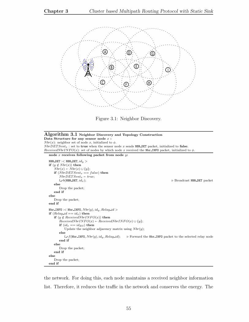
Chapter 3 Cluster based Multipath Routing Protocol with Static Sink
E
FH
G
B
A D
C
I
Figure 3.1: Neighbor Discovery.
Algorithm 3.1 Neighbor Discovery and Topology ConstructionData Structure for any sensor node x :Nbr(x): neighbor set of node x, initialized to φ.NbrDETSentx : set to true when the sensor node x sends NBR DET packet, initialized to false.ReceivedNbrINFO(x): set of nodes by which node x received the Nbr INFO packet, initialized to φ.
node x receives following packet from node y:
NBR DET :< NBR DET, idy >if (y /∈ Nbr(x)) then
Nbr(x) � Nbr(x) ∪ {y};if (NbrDETSentx == false) then
NbrDETSentx � true;l rb(NBR DET, idx); . Broadcast NBR DET packet
elseDrop the packet;
end ifelse
Drop the packet;end if
Nbr INFO :< Nbr INFO, Nbr(y), idy , Relay id >if (Relay id == idx) then
if (y /∈ ReceivedNbrINFO(x)) thenReceivedNbrINFO(x) � ReceivedNbrINFO(x) ∪ {y};if (idx == idBS) then
Update the neighbor adjacency matrix using Nbr(y);else
l rf(Nbr INFO, Nbr(y), idy , Relay id); . Forward the Nbr INFO packet to the selected relay nodeend if
elseDrop the packet;
end ifelse
Drop the packet;end if
the network. For doing this, each node maintains a received neighbor information
list. Therefore, it reduces the traffic in the network and conserves the energy. The
55

Chapter 3 Cluster based Multipath Routing Protocol with Static Sink
F H
GA D
C
IB
Nbr_IN
FO
Nbr_INFO
Nbr_INFO
Nbr_INFO
Nbr_IN
FO
Nbr_INFO N
br_INFO
Nbr_IN
FO
Nbr_INFONbr_INFO
Nbr_INFONbr_INFO
Nbr_INFO Nbr_INFO
Nbr_IN
FO
Figure 3.2: Nodes send the Nbr INFO packet to the base station.
BS A B C D E F G H I
BS 0 1 1 1 0 0 0 0 0 0A 1 0 1 0 1 0 0 0 0 0B 1 1 0 1 1 1 1 0 0 0C 1 0 1 0 0 0 1 0 0 0D 0 1 1 0 0 1 0 1 0 0E 0 0 1 0 1 0 1 1 1 0F 0 0 1 1 0 1 0 0 1 0G 0 0 0 0 1 1 0 0 0 1H 0 0 0 0 0 1 1 0 0 0I 0 0 0 0 0 0 0 1 1 0
Table 3.1: Neighbor Adjacency Matrix.
base station creates the neighbor adjacency matrix when it receives the Nbr INFO
from the sensor nodes. Neighbor adjacency matrix is shown in Table 3.1. It is
a (n + 1) × (n + 1) matrix, where n is the number of nodes in the network and
a base station. The neighbor adjacency matrix shows the network topology and
connectivity of the nodes. Based on neighbor adjacency matrix, the base station
selects the cluster heads and routing paths from each cluster head to the base
station.
3.3.2 Cluster Head Selection and Cluster Formation
After neighbor discovery and topology construction, the formation of the
cluster is started. Initially, all nodes’ energy levels are the same. After the
formation of the neighbor adjacency matrix, the base station will compute and
monitor the residual energy of each node. The base station chooses a certain
56

Chapter 3 Cluster based Multipath Routing Protocol with Static Sink
number of cluster heads in the network using the following conditions:
1. Two cluster heads should not be neighbor to each other,
Let CH is a set of all cluster heads and x ∈ CH
Nbr(x) is a set of one hop neighbors of x
if (y ∈ Nbr(x)) then
y /∈ CH . This is the first condition for any node to be a cluster head
end if
2. the residual energy (Er) of each cluster head should be greater than
threshold value.
Let Ethreshold is the threshold energy and
Erx is the residual energy of node x
if (Erx ≥ Ethreshold) then
x ∈ CH . This is the second condition for any node to be a cluster
head
end if
3. and each cluster head should have at least k2number of nodes as neighbor.
Let a is the alive nodes and
m is the optimal number of cluster heads in the network
Then, k = a−mm
. k is the average number of nodes in a cluster in the
ideal case
So that, Nbr(x) ≥ k2
. This is the third condition for any node to be a
cluster head
The selection of a cluster head depends on two independent factors; one is the
residual energy (Er), and another is the degree of the node, i.e., the number of
neighbor nodes.
Lemma 3.1. At most one cluster head is selected in the radio range R.
Proof. In CMRP, the sink selects the cluster head with the condition that two
cluster head will not be the neighbor of each other. In other words, in the cluster
57

Chapter 3 Cluster based Multipath Routing Protocol with Static Sink
head range R there should not be any other cluster head. Sink selects the cluster
head based on the neighbor list of each node. Let CH is the set of all cluster
heads and a node x ∈ CH , Nbr(x) is the set of one-hop neighbors of x.
if (y ∈ Nbr(x)) then
y /∈ CH
Lemma 3.2. Expected number of nodes within the cluster head radio range R is⌈(
πR2
|A|
)
× n⌉
.
Proof. Let, nexp is the expected number of the nodes within the cluster range
R. The area a cluster head can cover is πR2, and the network area are defined as
A(m×m). If the number of sensor nodes in the network is n, then the expected
number of nodes within the cluster head radio range is
nexp =
⌈(
πR2
|A|
)
× n
⌉
(3.3)
Lemma 3.3. CHreq number of cluster heads can cover the entire network.
Proof. Considering Lemma 3.2, the expected number of nodes within the network
is nexp. Let, CHreq is the required number of cluster heads to cover the entire
network then,
n = CHreq + (CHreq × nexp) (3.4)
n = (1 + nexp)× CHreq (3.5)
so,
CHreq =n
(1 + nexp)(3.6)
Hence, The entire network can be covered using CHreq number of cluster heads.
After selecting the cluster head, the base station determines the path between
the cluster head and the base station. The base station refers to the neighbor
adjacency matrix and ensures the following selection criteria for routing path:
58

Chapter 3 Cluster based Multipath Routing Protocol with Static Sink
1. The residual energy of the sensor node in the path should be greater than
the threshold value,
Let P is a set of nodes in the path
and Erx is the residual energy x ∈ P then
Erx ≥ Ethreshold . This is the first condition for routing path selection
2. and the total energy consumption of the routing path should be minimum.
Let | P | is the number of nodes in the path and
{P1, P2, P3, ....Pj} are the available paths from the cluster head to the
base station.
So, P = min1≤i≤j(| Pi |) . This is the second condition for routing path
selection
Algorithm 3.2 Cluster Head IntimationData Structure for any sensor node x :PATH(x): set of sensor nodes involved in the path between the node x and the base station.RTable(x) : the routing table maintained by each relay node having two columns cluster head id and next hop,initialized to φ.
node x receives following packet from node y:
CH INT :< CH INT, idy , PATH(ch), idch >if (idch == idx) then
l rf(ACK, idx, next hop); . Forward the ACK packet to the base stationelse
if (x ∈ PATH(ch) && idch /∈ RTable(x)) thenUpdate the RTable(x) by adding cluster head id as idch and next hop as idy ;l rb(CH INT, idx, PATH(ch), idch); . Broadcast CH INT packet
elseDrop the packet;
end ifend if
ACK :< ACK, idy , next hop >if (next hop == idx) then
if (idx == idBS) thenT ime out← false;
elseLook up the RTable(x) and find the next hop of cluster head y;l rf(ACK, idy , next hop); . Forward the ACK packet towards the base station
end ifelse
Drop the packet;end if
To notify the sensor nodes that have been chosen as a cluster head, the base
station unicasts the intimation packet (CH INT) to the cluster heads using the
selected path as illustrated in the Algorithm 3.2. The CH INT packet follows the
path and reaches the cluster head. The sensor nodes involved in the path make a
59

Chapter 3 Cluster based Multipath Routing Protocol with Static Sink
reverse link towards the sink to relay the data from the cluster head. When the
cluster head receives the CH INT packet, it sends back an acknowledgment (ACK)
packet to the base station. The ACK packet follows the same reverse path from
where CH INT packet came. The base station selects another path if it does not
receive the ACK packet from the cluster head within a predefined time duration.
Afterwards, cluster head broadcasts the advertisement packet to form a
cluster as illustrated in the Algorithm 3.3. Nodes that receive more than one
advertisement will choose the cluster head based on higher RSSI (Received Signal
Strength Indication). After selecting the cluster head, a node sends the joining
request in the format CH JOIN packet. The cluster head receives similar CH JOIN
packets from each interested node. After receiving all the joining requests, the
cluster head transmits the information of the cluster members to the base station.
For reducing the congestion, the cluster head generates the time-slot schedule for
the cluster members based on Time Division Multiple Access (TDMA) [101] and
send to the cluster members. The TDMA time-slot is used for the collision-free
communication between the cluster member and the cluster head.
Algorithm 3.3 Cluster FormationData Structure for any sensor node x :RSSI(x): set of received signal strength of the sender nodes, initialized to φ.CHSelectedx: set to true when the sensor node x selected the cluster head, initialized to false.ChMbr(x): set of cluster members of any cluster head x, initialized to φ.
node x receives following packet from node y: where x /∈ CH and y ∈ CH
CH ADV :< CH ADV, idy >;RSSI(x)← RSSI(x) ∪ RSSIy;After receiving all CH ADV, node x chooses a node with highest received signal strength as its cluster head.CHSelectedx ← true;l rf(CH JOIN, idx, idch); . Send the join request to the cluster head
node x receives following packet from node y: where x ∈ CH and y /∈ CH
CH JOIN :< CH JOIN, idy , idch >if (idx == idch) then
ChMbr(x)← ChMbr(x) ∪ y;After receiving all CH JOIN, node x sends the ChMbr(x) to the base station.Broadcast the time-slot schedule to the cluster members.
elseDrop the packet;
end if
60

Chapter 3 Cluster based Multipath Routing Protocol with Static Sink
Lemma 3.4. The cluster formation requires O(n) control messages.
Proof. At the beginning, each node broadcasts a NBR DET packet. Thus, there
are n messages in the network. Each node transmits its neighbor information to
the sink that again takes n messages. Each cluster member broadcast a CH JOIN
packet to join the cluster head. Suppose the number of generated cluster heads
are α. So the total number of join request is (n−α) and for time-slot α messages
are required by the cluster heads. Thus the total number of control messages in
cluster formation requires n + (n − α) + α + α = 2n + α. Therefore, the overall
complexity of the control message in the network for cluster formation is O(n).
Lemma 3.5. Etotal =∑
((ECH × (α)) + (ECM × (1− α) )) is the total energyconsumption in the network.
Proof. In CMRP, each node is divided into two category cluster head and cluster
members. Cluster members transmit their data to the cluster head, and cluster
head aggregates the data and transmits to the sink. The individual cluster head
consumes ECH energy in the transmission, reception and aggregation. Cluster
member consumes ECM energy in the transmission, reception and sleeping. Let
α is the number of cluster head in the network, and then the total energy
consumption in the network is
Etotal =∑
((ECH × (α)) + (ECM × (1− α) )) (3.7)
3.3.3 Data Transmission
The cluster member transmits the generated data to the cluster head based on
the given time slot and then changes the operational mode to sleep mode. The
sensor node wakes up in the next time slot to transmit the data. In this way,
the protocol helps in conserving the energy of the sensor nodes. The cluster head
aggregates the data and sends to the base station through the selected path. All
intermediate relay nodes refer to the routing table for the next node to forward the
61

Chapter 3 Cluster based Multipath Routing Protocol with Static Sink
data. When the data reaches the base station, an acknowledgment packet is sent
back to the cluster head. If the cluster head does not receive the acknowledgment
from the base station, it re-transmits the data. The base station monitors the
residual energy of each node in the network as it has the entire information of
network topology. If base station finds the residual energy of any node below the
threshold value, it selects another available path for that cluster head.
3.3.4 Re-clustering and Rerouting
The base station initiates the process of re-clustering and rerouting. It monitors
the residual energy of each sensor node in the network to balance the load among
the sensor nodes. If the residual energy falls below the threshold value, the node
initiates re-clustering or rerouting based on its role. If that node is a relay node of
any path, then the base station selects another available path to exclude that node.
If the node is a cluster head, then the base station selects another cluster head
and the corresponding path. This method increases the lifetime of the networks.
The node is having the residual energy below the threshold, neither take part in
routing nor become a cluster head, but only operate as the cluster member.
3.4 Simulation Results
Through the simulation, the proposed CMRP performance is analyzed and
compared with the existing protocols such as Fault Diagnosis based Clustering
and Multipath routing protocol (FDCM) [15] and Practical Passive Cluster
based Multipath Protocol (PPCMP) [53]. The performances of the protocols
are compared based on the metrics such as control packet overhead, energy
consumption, packet delivery ratio and network lifetime as specified in Chapter 2.
The intensive set of simulation is performed using the Castalia (v3.2) simulator
and based on the parameter illustrated in Table 3.2.
62

Chapter 3 Cluster based Multipath Routing Protocol with Static Sink
Parameter Name Value
Network area 500 × 500 meter2
Number of sensor nodes 100Data packet size 512 bytesControl packet size 32 bytesInitial energy 1JEelec 50 nJ/bitεfs 10 pJ/bit/m2
εmp 0.0013 pJ/bit/m4
d0 87 metersEproc 5 nJ/bitElow 0.2 nJ/secSimulation time 400 secMAC protocol TMAC
Table 3.2: Simulation Parameters
3.4.1 Average Control Packet Overhead
The control packet overhead by the various protocols is shown in Figure 3.3.
50 100 150 200 250 300 350 400
0.1
0.2
0.3
0.4
0.5
Simulation time (s)
Ave
rag
e C
on
tro
l P
ackets
Ove
rhe
ad
(J)
Proposed
FDCM
PPCMP
Figure 3.3: Average Control Packet Overhead.
It is observed that the control packet overhead is less for the proposed protocol
(CMRP) as compared to PPCMP and FDCM. This is because the proposed
scheme neither uses flooding nor involves the entire network in selecting the
cluster heads and multipath. The sink itself selects the cluster heads and the
routing paths. However, PPCMP constructs multipath by flooding the control
packets over the network. This is the major cause for the increase in control
packets overhead. Further, if any node becomes the source node, the multipath
63

Chapter 3 Cluster based Multipath Routing Protocol with Static Sink
is reconstructed. This is an additional overhead of the protocol. In the cluster
formation phase of FDCM, the exchange of test request and reply for testing the
faulty node is an overhead. In multipath construction, the control packets are
broadcasted in the increased range of 2R that also consumes more energy.
3.4.2 Average Energy Consumption
The average energy consumption by various protocols is illustrated in Figure
3.4. The average energy consumption by the proposed protocol (CMRP) is less
as compared to PPCMP and FDCM. PPCMP uses the optimal path to transmit
the data. However, due to increased control packet overhead, the average energy
consumption is more. In FDCM, the control packet overhead is more, and the
aggregated data are transmitted through the cluster heads with the range of
2R. This increases the overall energy consumption as it takes twice the power
to transmit the data as compared to the other protocol. However, in the proposed
protocol, the control overhead is less as the sink itself selects the optimal path for
the data transmission. Therefore, the average energy consumption is least.
50 100 150 200 250 300 350 400
0.2
0.3
0.4
0.5
0.6
Simulation time (s)
Ave
rag
e E
ne
rgy C
on
sum
ptio
n(J
)
Proposed
FDCM
PPCMP
Figure 3.4: Average Energy Consumption.
3.4.3 Average End-to-End Latency
In the FDCM, due to available neighbor cluster head list the end-to-end delay
is less. However, in a situation where the network has to choose a new cluster
64

Chapter 3 Cluster based Multipath Routing Protocol with Static Sink
head, the selection process starts from the beginning, which increases the delay.
Whereas, for the proposed scheme, the alternative paths are available. The result
in Figure 3.5 shows that the end-to-end latency of the proposed scheme is less
than the PPCMP and marginally lesser than the FDCM.
30 40 50 60 70 80 90 100
0.2
0.25
0.3
0.35
0.4
0.45
0.5
Number of nodes
Da
ta d
eliv
ery
la
ten
cy (
s)
Proposed
FDCM
PPCMP
Figure 3.5: Average End-to-End Latency.
3.4.4 Packet Delivery Ratio
The packet delivery ratio of each protocol is depicted in Figure 3.6.
30 40 50 60 70 80 90 100
20
40
60
80
100
Number of nodes
Pa
cke
t d
eliv
ery
ra
tio
(%)
Proposed
FDCM
PPCMP
Figure 3.6: Packet Delivery Ratio.
PPCMP uses the node-disjoint multipath routing, which increases the
reliability hence the delivery ratio also increases. The FDCM does not take such
65

Chapter 3 Cluster based Multipath Routing Protocol with Static Sink
20 40 60 80 100 120 140 160 180 200
40
60
80
100
Number of nodes
Pa
cke
t d
eliv
ery
ra
tio
(%)
Proposed
FDCM
PPCMP
Figure 3.7: Packet Delivery Ratio (1800 sec and 200 nodes).
precautions when the path fails between the source and the sink. In fact, it
chooses the neighbor cluster head from the available list without knowing the
current residual energy. Hence, the reliability of the FDCM decreases. However,
in the proposed scheme (CMRP), the sink itself selects the path and monitors the
remaining energy of each node in the path. When it finds any node’s residual
energy below the threshold, it chooses another path for data transmission. Hence,
the data loss is negligible.
In the Figure 3.6, it has been also observed that the proposed protocol and
PPCMP gives almost the same packet delivery ratio up to 80 sensor nodes. Beyond
80 nodes the proposed protocol gives slightly better result. To further examine
the performance of the proposed protocol with existing protocol the simulation
has been performed with the simulation time 1800 seconds and up to 200 sensor
nodes. From the result shown in Figure 3.7, it has been found that the proposed
protocol behaves uniformly and gives better packet delivery ratio than the existing
protocols.
3.4.5 Network Lifetime
Figure 3.8 depicts the network lifetime for various protocols. It is clearly
illustrated that the network lifetime of the proposed scheme is greater than the
FDCM and PPCMP. The reason behind this is, it consumes fewer control packets
66

Chapter 3 Cluster based Multipath Routing Protocol with Static Sink
and balances the load among the sensor nodes.
50 100 150 200 250 300 350 400
40
60
80
100
Simulation time(s)
Nu
mb
er
of
nod
es a
live
Proposed
FDCM
PPCMP
Figure 3.8: Network Lifetime.
3.5 Summary
This chapter proposed an energy-efficient routing scheme using the clustering
and multipath technique called CMRP. The workload on the sensor nodes are
alleviated by giving more responsibility to the base station. The multipath gives
more reliability to the network, and it increases the delivery ratio and decreases the
latency. In addition to that, cluster-based data collection reduces the traffic and
energy consumption and also increases the lifetime of the network. The simulation
result shows that the proposed protocol outperforms the existing FDCM and
PPCMP protocols.
67

Tree based Routing Protocol with Mobile Sink
Introduction
System Model
The Proposed Protocol
Simulation Results
Summary

Chapter 4
Tree based Routing Protocol withMobile Sink
4.1 Introduction
In static sink environment, sensor nodes close to sink always act as the relay
nodes. Relay nodes deliver the data to the sink and thus, consume more energy
as compared to other nodes that are far from the sink, consequently, they die.
It creates hotspots [102, 103] in the sink vicinity, and the network gets detached.
Although remaining sensor nodes still have their energy and operative. Such,
situation is called “crowded center effect” [60] or “energy hole/hotspot problem”
[102,103]. Sink mobility prolongs the network lifetime by diminishing the hotspot
problem.
Apart from hotspot solution, the mobile sink has many advantages over
the static sink such as load balancing, shorter data dissemination path and
better handling of the sparse or disconnected network. Frequent change of the
neighboring nodes of the sink leads to balance the load of the network. Shorter
data dissemination path provides longer network lifetime by increasing throughput
and decreasing energy consumption [104].
The mobile sink moves within the network and collects data from the sensor
nodes. The movement of the sink may be a random, controlled or predefined
and makes the network dynamic in nature. A mobile sink is required to update
their location information in the network. This process consumes more energy
of the network. So the routing protocols with the static sink are not suitable
69

Chapter 4 Tree based Routing Protocol with Mobile Sink
with the mobile sink. However, efficient broadcasting and routing technique can
reduce this power consumption up to a certain extent. It is a very challenging
task to manage the sink mobility and develop an efficient routing technique. This
challenge motivates to develop the routing protocol with mobile sink, which uses
less energy to manage the mobility of the sink.
The main flaws in the existing routing protocols with mobile sink [67, 69–71]
are higher routing overhead and shorter lifetime. In this chapter, a Tree based
Data Dissemination protocol with mobile sink (TEDD) is proposed to overcome
the above flaws. In this protocol, any sensor node can disseminate the data to the
sink via a tree. The tree is independent of the sink mobility. In the tree structure,
the leaf node is known as non-relay, and the non-leaf node is called relay node.
TEDD manages the mobility of the sink and balances the load among the sensor
nodes to maximize the lifetime. The system model of the proposed protocol is
discussed in Section 4.2. The working principle of the TEDD is presented in
Section 4.3. The simulation results and analysis are explained in Section 4.4. In
Section 4.5 the chapter is summarized.
4.2 System Model
4.2.1 Assumptions
The following assumptions are considered for the proposed protocol.
• Sensor nodes are all stationary after deployment.
• The sink is moving within the network.
• The sensors are randomly deployed in the network field with uniform
distribution.
• The base station possesses unlimited memory, computation and battery
power.
• Each node possesses its id and can calculate the residual energy.
• Sensor nodes are homogeneous and have the same capabilities.
70

Chapter 4 Tree based Routing Protocol with Mobile Sink
• Sensor nodes have limited energy.
• Links are symmetric, i.e., the data speed or quantity is the same in both
directions, averaged over time.
4.2.2 Network Model
It is considered that a wireless sensor network that consists of n number of
sensor nodes and a mobile sink. The protocol generates a tree T from the sensor
nodes. It can be represented as a graph G(V,E) where V = {v1, v2, ...vn} is the
sensor nodes and E are the links between a node set (vi, vj) where vi, vj ∈ V . The
tree construction is independent of the sink position. The sink is moving within
the network with the varying speed of 5 to 30meter/second. The Pause time
(δ) for sink to collect the data is 5 seconds. The total energy consumption by
the sensor node in the network is the same as specified in Chapter 2. The sensor
nodes are categorized into two types relay node and non-relay node. The relay
node forwards the data from the other sensor nodes, whereas non-relay node only
transmits its data to their parent relay node.
4.2.3 Mobility Model
In the simulation, to show the impact of the sink mobility, the random waypoint
mobility model [105] has been considered.
• Random Waypoint model:
Random Waypoint model is a “benchmark” mobility model for Ad-Hoc
networks to evaluate the performance of the routing protocol. The random
waypoint model is used for the sink mobility in wireless sensor networks. It
randomly generates the next position in between Pmin and Pmax. Sink travels
towards its succeeding position with constant speed or random speed. When
the sink node reaches the next position, it pauses for the time duration called
the Pause time (δ).
The random waypoint model does not consider the previous position to
calculate the next position. Hence it does not generate the relative motion.
71

Chapter 4 Tree based Routing Protocol with Mobile Sink
4.3 The Proposed Protocol
The proposed protocol (TEDD) creates the tree in the network. There are two
categories of the nodes in the tree: one is the relay node (RN), and the other is the
non-relay node (non − RN). The relay node is responsible to handover the data
from the nodes to its next relay node. The non-relay nodes can only communicate
through a relay node. Therefore, it is a unidirectional communication. However,
the communication is bi-directional between two relay nodes. The tree topology
changes when the role of the node changes from a relay to non-relay or from
non-relay to a relay node. To rotate the responsibility of the relay node each
node’s residual energy is considered.
The sink is mobile and collects the data from the source nodes through the
gateway node. The gateway node may be a relay node or a non-relay node. The
sink selects the gateway node based on the criteria mentioned in Section 4.3.2.
The sink periodically transmits a small beacon to make the connection alive with
the gateway node. If the sink moves out of the range of the current gateway node,
then it selects another node as the gateway node. The rotation of the gateway
node can overcome the problem of the energy hole [61]. The proposed protocol
consists of various phases such as neighbor discovery, tree construction and relay
node selection, and data transmission.
4.3.1 Neighbor Discovery
It is the initial phase of the proposed protocol in which each node finds its
neighbor nodes. As illustrated in Algorithm 4.1 the initiator node broadcasts the
NBR DET packet. It includes the node id of the sender and the willingness to be
the relay node with the format < NBR DET, idx,WILLx >. The sender nodes itself
decide the willingness based on its residual energy Er. If Er ≥ Ethreshold, WILLx
will be true otherwise false. Any node x receives the NBR DET packet does the
following operations:
• Checks for the existence of the sender node id, if not found, include the
sender node id in the Neighbor list Nbr(x).
72

Chapter 4 Tree based Routing Protocol with Mobile Sink
• Checks for the willing to be a relay node, if true, then include sender node
id to the candidate relay node list CRN(x).
• Checks if the NBR DET packet is broadcasted by the recipient node, if not,
then broadcast the packet with format < NBR DET, idx,WILLx > and make
NbrDETSentx as true.
Neighbor discovery phase is over as soon as each node broadcast their NBR DET
packet. At the end, each node gets the partial view of the network in the form of
neighbor information.
Algorithm 4.1 Neighbor DiscoveryData Structure for any sensor node x :Nbr(x): neighbor set of node x, initialized to φ.CRN(x) : the set of neighbors of node x, which are willing to be the relay node, initialized to φ.WILLx : either true or false depends on the willingness of node x to become a relay node.NbrDETSentx : set to true when the sensor node x sends NBR DET packet, initialized to false.
node x receives following packet from node y:
NBR DET : < NBR DET, idy ,WILLy >if (y /∈ Nbr(x)) then
Nbr(x) � Nbr(x) ∪ {y};if (WILLy == true) then
CRN(x) � CRN(x) ∪ {y};end ifif (NbrDETSentx == false) then
NbrDETSentx � true;l rb(NBR DET, idx,WILLx); . Broadcast NBR DET packet
elseDrop the packet;
end ifelse
Drop the packet;end if
-
(a) Initial view of tree construction.
-
(b) Final view of tree construction.
Figure 4.1: Tree construction steps shown in (a) and (b)
73

Chapter 4 Tree based Routing Protocol with Mobile Sink
Algorithm 4.2 Tree Construction and Relay node SelectionData Structure for any sensor node x :Children(x) : children set of node x, initialized to φ.Parent(x) : parent of node x, initialized to φ.RNnodes : set of relay nodes in the network.Parent Selectedx : set to true once the sensor node x selects its parent, initialized to false.T MSGSentx : set to true once the sensor node x sends T MSG packet, initialized to false.CRN(x) : the set of neighbors of node x, which are willing to be the relay node, initialized to φ.
node x receives following packets from node y ∈ Nbr(x):
T MSG : < T MSG, idy , Parent(y) >if (idx ∈ Parent(y)) then
Children(x) � Children(x) ∪ {idy};RNnodes � RNnodes ∪ {x}; . node x declare itself as a relay nodeDrop the packet;
else if (Parent Selectedx == false && y ∈ CRN(x)) thenParent(x) � y;Parent Selectedx � true;if ((T MSGSentx == false)) then
T MSGSentx � true;l rb(T MSG, idx, Parent(x)); . Broadcast T MSG packet
elseDrop the packet;
end ifelse
Drop the packet;end if
. Timeout occur to the node y when the time duration expire for the tree construction phase andTIMEOUTy become true.if (TIMEOUTy == true) then
if (Parent Selectedy == false) thenl rb(T ERR, idy); . Broadcast T ERR packet
end ifend if
T ERR : < T ERR, idy >if (Parent Selectedx == true) then
T MSGSentx � true;l rb(T MSG, idx, Parent(x)); . Broadcast T MSG packet
elseDrop the packet;
end if
4.3.2 Tree Construction and Relay Node Selection
After getting the neighbor list, each node has the neighbors’ information such
as id and the willingness to become the relay node. The tree construction and relay
node selection phase is initiated by using the neighbor information. As depicted
in Algorithm 4.2, the initiator node starts the tree construction by broadcasting
the T MSG control packet. The node receives the following packets during the tree
construction and relay node selection phase:
• T MSG: In the process of tree construction T MSG control packet is used. The
format of the packet is < T MSG, idy, Parent(y) >. Here idy is the sender
node id and Parent(y) is its parent node id. Any node x receives the T MSG
74

Chapter 4 Tree based Routing Protocol with Mobile Sink
packet performs following operations:
– If the sender’s parent node id is the same as the recipient id, then
include the sender id in the children list Children(x) and include the
recipient id into the relay node list RNnodes.
– If it has not selected any parent, and sender belongs to the list of relay
node RNnodes then, select sender node as its parent.
– If T MSGSent is false then, broadcast T MSG packet with modified
parameter to the network.
• T ERR: Timeout occurs to the node when the time duration expires for the
tree construction phase. Any node y checks for its parent node if it does
not exist, then a node y broadcasts an error message T ERR to its neighbor
nodes. The receiver node performs following operation:
– It initiates tree construction by broadcasting T MSG if it belongs to the
tree, otherwise drop the packet.
In this way, the rest of the nodes that do not belong to the tree will get an
opportunity to connect with the tree as shown in Figure 4.1. At the end of tree
construction, each non-relay node makes a reverse link to its parent relay node for
data transmission as shown in Figure 4.2(a).
-
(a) Link reversal process.
- -
(b) Sink mobility management and Gatewaynode selection.
Figure 4.2: Link reversal and Sink mobility management.
75

Chapter 4 Tree based Routing Protocol with Mobile Sink
- -
Figure 4.3: Path construction for gateway node and Data transmission.
The mobile sink moves within the network using the random waypoint mobility
model. It collects the data from the sensor nodes. In TEDD, any node closest to
the sink will be selected as the gateway node. If the selected gateway node is not
a relay node, then it selects its parent relay node as the gateway. This process is
illustrated in Figure 4.2(b). The gateway disseminates the information about the
sink in the network through the relay nodes. The relay node establishes a reverse
link to the relay node from where it receives the sink information as shown in
Figure 4.3.
4.3.3 Data Transmission
The responsibility of the relay node is to forward the data to the next relay
node. Any node can sense the data from the environment and transmits to the
next relay node. Node x receives the following packet during the data transmission
phase from node y as described in Algorithm 4.3.
• DATA: Each node in the network senses the environment, generates the
data and transmits it towards the next relay node with the format <
DATA, idy, sec noy >. Here idy is the id of sender node y and sec noy is
the data sequence number of the node y. Any node that receives the DATA
packet performs following actions:
– If the receiver node is a relay node, and it receives any duplicate data,
then it drops that data packet.
76

Chapter 4 Tree based Routing Protocol with Mobile Sink
– If the receiver node is a gateway node, then forwards the data packet
to the sink else forwards the DATA packet to its next relay node.
– Add the sender id and data sequence number to the list Send Data(x).
Algorithm 4.3 Data TransmissionData Structure for any sensor node x :Send Data(x) : node x add the pair of id and sec no after receiving the DATA packet, initialized to φ.Gateway : node selected by the sink for data reception.
node x will receive following packet from node y ∈ Nbr(x):
DATA : < DATA, idy , sec noy >if (x ∈ RNnode) then
if (< idy, seq noy > /∈ Send Date(x)) thenif (x == Gateway) then
Send Data(x) � Send Data(x) ∪ {y, sec noy};Forward DATA packet towards the sink;
elseSend Data(x) � Send Data(x) ∪ {y, sec noy};Forward DATA packet to its neighbor relay node towards gateway
end ifelse
Drop the packet;end if
elseDrop the packet;
end if
Lemma 4.1. The message complexity of the TEDD is O(nk).
Proof. Let n number of sensor nodes are deployed in the network. According to
Lemma 2.2, for neighbor discovery phase message complexity of a sensor node is
O(k), where k is the number of neighbors and k < n. For the tree construction,
each sensor node communicates (1 + k) messages. Let ‘r’ number of relay nodes
are used within the network, where r < n. The message complexity for the mobile
sink management is O(r) so that each node can send their data to the sink. The
total message across the network is represented as (nk+n(1+ k)+ r). Hence, the
message complexity of the TEDD protocol is O(nk).
4.4 Simulation Results
The simulation is performed for the TEDD, and the existing protocols such
as probabilistic data dissemination protocol called SUPPLE [70], Multi-Point
Relay based routing (SN-MPR) [71] and Adaptive Reversal Tree (ART) [67] to
examine the energy consumption, end-to-end latency, data delivery ratio and
77

Chapter 4 Tree based Routing Protocol with Mobile Sink
network lifetime of the network as specified in Chapter 2. The performance of
the proposed protocol is evaluated and compared the result with the existing
tree-based protocols. For the fair comparison, the simulation parameters are
equivalent to the existing protocols. The impact of the random waypoint mobility
model in energy consumption is observed. The intensive set of simulation is
performed using the Castalia (v3.2) simulator and based on the parameters listed
in Table 4.1.
Parameter Name Value
Network area 500 × 500 meter2
Number of sensor nodes 200Data packet size 512 bytesControl packet size 32 bytesInitial energy 1Jδ 5 secSink speed (5, 10, 15, 20, 25, 30) m/secMobility Model Random WaypointEelec 50 nJ/bitεfs 10 pJ/bit/m2
εmp4 0.0013 pJ/bit/m4
d0 87 metersElow 0.2 nJ/secSimulation time 400 secMAC protocol TMAC
Table 4.1: Simulation Parameters.
4.4.1 Average Control Packet Overhead
As observed from the Figure 4.4, that the tree reconstruction and sink
management cost is very less in the proposed protocol as compared to the other
protocols. In ART, the entire network should know the current position of the sink.
The tree rebuilt with the nearest node to the sink as root. The tree reconstruction
cost of ART depends on the affected area. However, in SN-MPR the root of the
tree is the sink. Like ART, SN-MPR also rebuilt the tree when the sink moves.
However, the new position of the sink only be known to the selected nodes. So
the control overhead of the SN-MPR is less than the ART.
In SUPPLE, the tree is constructed, and storing nodes are selected. The storing
nodes temporarily store the data from the source nodes. When the sink comes
78
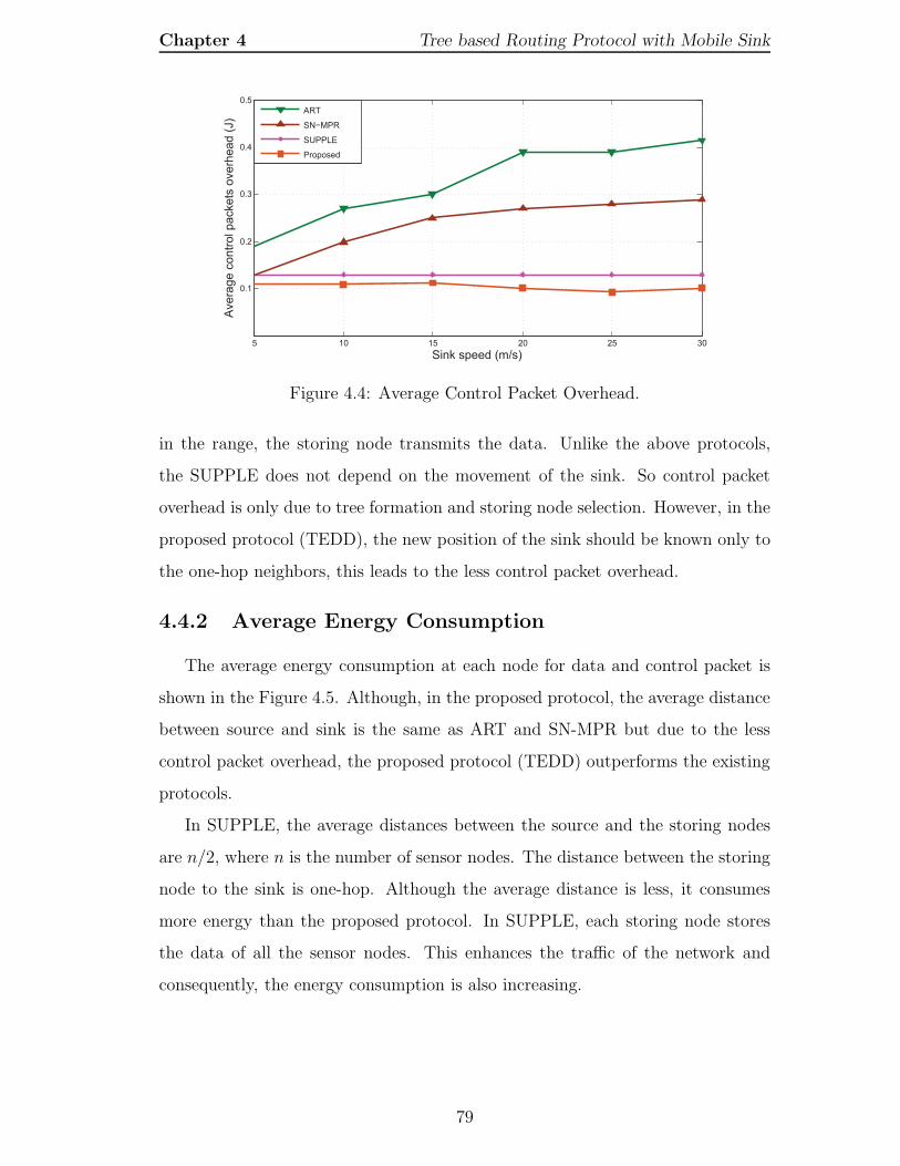
Chapter 4 Tree based Routing Protocol with Mobile Sink
5 10 15 20 25 30
0.1
0.2
0.3
0.4
0.5
Sink speed (m/s)
Ave
rag
e c
on
tro
l p
acke
ts o
ve
rhe
ad
(J)
ART
SN−MPR
SUPPLE
Proposed
Figure 4.4: Average Control Packet Overhead.
in the range, the storing node transmits the data. Unlike the above protocols,
the SUPPLE does not depend on the movement of the sink. So control packet
overhead is only due to tree formation and storing node selection. However, in the
proposed protocol (TEDD), the new position of the sink should be known only to
the one-hop neighbors, this leads to the less control packet overhead.
4.4.2 Average Energy Consumption
The average energy consumption at each node for data and control packet is
shown in the Figure 4.5. Although, in the proposed protocol, the average distance
between source and sink is the same as ART and SN-MPR but due to the less
control packet overhead, the proposed protocol (TEDD) outperforms the existing
protocols.
In SUPPLE, the average distances between the source and the storing nodes
are n/2, where n is the number of sensor nodes. The distance between the storing
node to the sink is one-hop. Although the average distance is less, it consumes
more energy than the proposed protocol. In SUPPLE, each storing node stores
the data of all the sensor nodes. This enhances the traffic of the network and
consequently, the energy consumption is also increasing.
79

Chapter 4 Tree based Routing Protocol with Mobile Sink
5 10 15 20 25 30
0.3
0.4
0.5
0.6
Sink speed (m/s)
Ave
rag
e e
ne
rgy c
on
su
mp
tio
n (
J)
ART
SN−MPR
SUPPLE
Proposed
Figure 4.5: Average Energy Consumption.
4.4.3 Average End-to-End Latency
The latency mainly depends on the duration of finding the valid path between
source and sink. Figure 4.6 presents the average end-to-end latency with various
sink speeds using the random waypoint mobility model. The time required to
reconstruct the tree based on the new position of the sink, cause the delay in ART
and SN-MPR. In SN-MPR, the affected area is less than the ART. So ART causes
more end-to-end latency than SN-MPR.
In SUPPLE, the sensor data is temporarily stored in the storing nodes. The
storing nodes wait for the mobile sink to come within the territory. It causes more
end-to-end latency than the above protocols. Whereas the proposed protocol
(TEDD) takes less cost and time to manage the mobility of the sink.
4.4.4 Packet Delivery Ratio
Figure 4.7 presented the data delivery ratio with different sink speeds.
SUPPLE performed well because the distance between the sink and storing node
is one-hop. The result of SN-MPR is also good due to the less affected area
and efficient recovery technique. The success ratio for ART decreases as the sink
speeds rise. The higher sink speed increases the frequency of the link failure, which
causes data loss. However, the proposed protocol is robust, i.e., the link always
maintained between the source and the sink. Hence, the data delivery ratio is
80

Chapter 4 Tree based Routing Protocol with Mobile Sink
5 10 15 20 25 30
0.01
0.02
0.03
0.04
0.05
0.06
0.07
Sink speed (m/s)
Avera
ge d
ata
deliv
ery
late
ncy (
s)
SUPPLE
Proposed
Figure 4.6: Average End-to-End Latency.
more than existing protocols.
5 10 15 20 25 30
60
70
80
90
100
Sink speed (m/s)
Data
deliv
ery
ratio (
%)
ART
SN�MPR
SUPPLE
Proposed
Figure 4.7: Packet Delivery Ratio.
4.4.5 Network Lifetime
In the network, the control packets are exchanged for neighbor maintenance,
relay node selection, tree construction, route establishment and maintenance. It
is called routing overhead and directly affects the lifetime of the network.
It has been observed from the resulting Figure 4.8 that the network lifetime of
the proposed scheme (TEDD) is higher than the ART and SN-MPR and slightly
better than SUPPLE. The reason behind this is, it consumes few control packets
and balances the load among the sensor nodes.
81

Chapter 4 Tree based Routing Protocol with Mobile Sink
50 100 150 200 250 300 350 400
120
140
160
180
200
Simulation Time (s)
Nu
mb
er
of
no
de
s a
live
ART
SN−MPR
SUPPLE
Proposed
Figure 4.8: Network Lifetime.
4.5 Summary
In this chapter, a distributed tree based data dissemination protocol called
TEDD has been proposed. The proposed protocol can efficiently manage the sink
mobility. The simulation is performed with the random waypoint mobility model.
The results are compared with the existing protocols such as SUPPLE, SN-MPR
and ART. It has been observed that the TEDD outperformed the above protocols,
because of its unique method to handle the sink mobility.
82

Dense Tree based Routing Protocol
with Mobile Sink
Introduction
System Model
The Proposed Protocol
Simulation Results
Summary

Chapter 5
Dense Tree based RoutingProtocol with Mobile Sink
5.1 Introduction
The sink mobility management in a routing protocol with controlled or
predictable mobility is quite easier than the random mobility. In other words, the
sensor node cannot predict the next position of the sink in random mobility. A
tree-based routing protocol called TEDD has been discussed in Chapter 4. TEDD
with random sink mobility has been performed better than the existing tree-based
protocols, but still there is some scope for improvement. The major flaws in the
TEDD protocol are increased control packet overhead and path length. When
the role of a relay node changes to a non-relay node then, TEDD is required
to reconstruct the tree. It escalates the control packet overhead and energy
consumption. The average routing path length of TEDD is greater than n/2,
where n is the number of sensor nodes in the network. The path length directly
depends on the number of relay nodes within the network.
In this chapter, a Dense Tree based Routing Protocol (DTRP) is proposed to
control the overhead and reduces the path length. The tree is constructed in such
a way that the number of relay node is much less than the non-relay node. Hence,
the path reduces and control packet overhead also decreases. The system model
of DTRP is described in Section 5.2. In Section 5.3 the working principle of the
proposed protocol is presented. The simulation results and analysis are discussed
in Section 5.4. In Section 5.5 the proposed protocol is summarized.
84

Chapter 5 Dense Tree based Routing Protocol with Mobile Sink
5.2 System Model
5.2.1 Network, Energy, and Mobility Model
In this chapter, the same network model and assumptions as specified in
Chapter 4 have been considered. The energy model for the sensor node is the same
as defined in Chapter 2. The Random Waypoint mobility model is considered for
the sink mobility.
5.3 Proposed Protocol
In this chapter, an energy-efficient Dense Tree based Routing Protocol (DTRP)
is proposed. In this protocol, the network is represented as a tree. Through the
tree, all nodes are connected to the network. In the network, the sensor nodes
create the tree independent of the sink position. The tree consists of two types of
nodes; relay node and non-relay node. A relay node is the sensor node selected by
another relay node. The relay node stores and forwards the data received by other
sensor nodes. The non-relay node only transmits their data to the relay node. The
sink node declares a relay node as the gateway node. The gateway node is the
interface between the sensor network and the sink. All relay node forwards the
data to the gateway node. The gateway node then transmits the received data to
the sink.
After the deployment, the initiator node broadcasts the control packet for
finding the one-hop neighbor node. Each node should broadcast once. In this way,
each node obtains the neighbor information. After neighbor discovery, initiator
node starts constructing the tree by selecting the relay node. Each non-relay node
chooses the parent relay node to send the data. The links between two relay nodes
are bidirectional, whereas non-relay node to relay node is unidirectional as shown
in Figure 5.1. When the sink wants to collect the data, it selects a gateway node in
its territory from the relay node set. Each relay node selects their neighbor relay
node to transmit the data to the gateway node as illustrated in Figure 5.2(a).
The proposed protocol consists of various phases such as neighbor discovery, tree
85

Chapter 5 Dense Tree based Routing Protocol with Mobile Sink
construction and relay node selection, mobile sink management, data transmission,
and load balancing and tree reconstruction.
5.3.1 Neighbor Discovery
In the neighbor discovery, each node finds their neighbor nodes. They maintain
the list of neighbor. Each node broadcasts their willingness along with the id
to become the relay node. The willingness is based on the residual energy of
the node. So at the end of neighbor discovery phase each node consists of the
neighbor list Nbr(x) and candidate relay node list CRN(x). All nodes have the
partial information about the topology of the network. The detailed algorithm for
the neighbor discovery is described in Algorithm 5.1.
Algorithm 5.1 Neighbor DiscoveryData Structure for any sensor node x :Nbr(x) : neighbor set of node x, initialized to φ.CRN(x) : the set of neighbors of node x, which are willing to be the relay node (candidate relay node), initializedto φ.WILLx : either true or false depends on the willingness of node x to become a relay node.NbrDETSentx : set to true when the sensor node x sends NBR DET packet, initialized to false.
node x receives following packet from node y:
NBR DET : < NBR DET, idy ,WILLy >if (y /∈ Nbr(x)) then
Nbr(x) � Nbr(x) ∪ {y};if (WILLy == true) then
RN(x) � RN(x) ∪ {y};end ifif (NbrDETSentx == false) then
NbrDETSentx � true;l rb(NBR DET, idx,WILLx); . Broadcast NBR DET packet
elseDrop the packet;
end ifelse
Drop the packet;end if
The initiator node broadcast the NBR DET packet with their id and willingness.
The node that receives the packet performs the following operations:
• Checks if the receiver node id is not in the neighbor list, then adds the sender
id into the Nbr(x).
• Checks if the willingness of the sender node is true, then adds the preceding
node id into the candidate relay node list CRN(x).
86

Chapter 5 Dense Tree based Routing Protocol with Mobile Sink
• The recipient node broadcasts the NBR DET packet if it does not broadcast
before.
5.3.2 Tree Construction and Relay Node Selection
In the tree construction and relay node selection phase, the initiator node
selects the first candidate relay node as the relay node and deletes that node from
the candidate relay node list. It creates a T MSG packet with its id and selected
relay node id and broadcast it. The receiver node selects the sender id as parent
and next node for data transmission if not selected any parent previously as shown
in Figure 5.1(a). If the receiver node is the chosen relay node by the sender relay
node, then the receiver node deletes the sender id from the candidate relay node
list and changes its status from Non-RN node to RN node. Again, receiver node
selects the relay node from the candidate relay node list and broadcast the T MSG
packet to create the tree in the network. Each node has its parent node and next
relay node for data transmission as illustrated in Figure 5.1(b). If any node is not
connected with the tree, then it generates an error message ERR and broadcasts
it. If it receives the T MSG in response from the relay node, it joins the network by
selecting the parent and next relay node.
(a) Initial view of tree construction. (b) Final view of tree construction.
Figure 5.1: Tree construction steps shown in (a) and (b).
At the end of tree construction and relay node selection phase, each node
87

Chapter 5 Dense Tree based Routing Protocol with Mobile Sink
becomes the part of the tree. The relay node has an additional responsibility
to forward the data from the neighbor nodes (relay or non-relay nodes). The
non-relay node only transmits their data to the parent relay node. The Algorithm
5.2 presented the tree construction and relay node selection.
Algorithm 5.2 Tree Construction and Relay node SelectionData Structure for any sensor node x :Nbr(x): neighbor set of node x.Parentx : parent of node x.RNx : relay node selected by the node x.Parent Selectedx : set to true once the sensor node x selects its parent, initialized to false.CRN(x) : the set of neighbors of node x, which are willing to be the relay node (candidate relay node).TreeConstructionx : set to true once the sensor node x called the TreeConstruction() , initialized to false.next nodex: the relay node x selects the next relay node for data transmission.Statusx : set to RN , when the sensor node x has been selected as relay node, initialized to non-RN .
procedure TreeConstruction()RNx � CRN(x0);CRN(x) � CRN(x) − CRN(x0);l rb(T MSG, idx, RNx); . Broadcast T MSG packet
end procedure
node x receives following packets from node y ∈ Nbr(x):
T MSG : < T MSG, idy , RNy >if (Parent Selectedx == false) then
Parentx � idy ;next nodex � idy;Parent Selectedx � true;if (idx == RNy) then
CRN(x) � CRN(x) − CRN(xidy );Statusx � RN ;if (TreeConstructionx == false) then
TreeConstructionx � true;TreeConstruction();
end ifelse
Drop the packet;end if
elseDrop the packet;
end if
. Timeout occur to any node x when the time duration expires for the tree construction phase andTIMEOUTy become true.if (TIMEOUTx == true) then
if (Parent Selectedx == false) thenl rb(T ERR, idx); . Broadcast T ERR packet
end ifend if
node x receives following packets from node y ∈ Nbr(x):
T ERR : < T ERR, idy >if (Statusx == RN) then
l rb(T MSG, idx, RNx); . Broadcast T MSG packetelse
Drop the packet;end if
In the algorithm, a procedure is defined called TreeConstruction(). It selects
the relay node from the candidate relay node list, updates the candidate relay
88

Chapter 5 Dense Tree based Routing Protocol with Mobile Sink
node list CRN(x) and broadcasts the T MSG for the tree construction. The node
that receives the T MSG packet does the following operations:
• Check if not it is selected the parent, then select sender node as the parent
and next nodex.
• Check if the receiver node is the relay node selected by the sender node, then
it updates the candidate relay node list.
• Updates the status to relay node (RN) and call the TreeConstruction()
procedure.
At the end of this phase when the timeout occurs for each node the algorithm
checks for the node that does not select any parent. That node generates an error
message ERR and broadcasts. If any relay node receives the ERR packet, it replies
with T MSG packet.
5.3.3 Mobile Sink Management
The sink is moving within the network. The random waypoint model for the
sink mobility has been considered. The mobile sink has been considered to reduce
the effect of energy hole problem [61]. The mobile sink moves within the network
and collects the data from the nodes through the gateway node as shown in Figure
5.2. The gateway works as an interface between the sensor network and the sink.
The sink chooses one of the relay nodes in its territory as a gateway node. The
gateway node broadcasts an acknowledgment (ACK) packet in the network. The
relay node selects their next relay node (next nodex) to send the data towards
the sink. The sink sends a STOP signal to the gateway node to halt the data
transmission just before it moves to the new position.
The detail description of the mobile sink management is discussed in Algorithm
5.3. When the mobile sink reaches to the new position, it broadcast a beacon
packet. The Beacon packet consists of sink id. The relay node that receives the
beacon should reply the sink with BeaconRelay packet. The BeaconReply packet
consists of its id and the sink id. When the sink receives first BeaconReply packet,
89

Chapter 5 Dense Tree based Routing Protocol with Mobile Sink
(a) Gateway node selection and Datatransmission.
(b) Sink mobility management.
Figure 5.2: Gateway selection and Data transmission and Sink mobilitymanagement.
it selects the sender relay node as the gateway and sends a Gateway packet. The
gateway packet consists of sink id and selected gateway node id. When the selected
gateway node receives the packet, it selects a next node as sink id and broadcasts
the acknowledgment (ACK) packet. The ACK packet consists of the sender id and
gateway node id. The recipient relay node performs the following operations:
• Checks if the ACK packet is not for the previous gateway node, then
• Selects the gateway node as newly selected gateway node and selects the
next node as sender node id.
• Forwards the ACK packet with its id and gateway node id.
In this way, each relay node selects the next relay node to transfer the data.
When the sink moves from its position, it sent a STOP signal to the gateway node.
The gateway node forwards the STOP signal to the network. So that the data loss
will decrease, and the delivery ratio will increase.
5.3.4 Data Transmission
When the relay node’s SendData flag is true, it can immediately start the
data transmission to the next relay node. The non-relay node can send their data
90

Chapter 5 Dense Tree based Routing Protocol with Mobile Sink
Algorithm 5.3 Mobile Sink ManagementData Structure for any sensor node x and sink:Gatewaysink : gateway node selected by the sink.next nodex: the relay node x selects the next relay node for data transmission.Statusx : set to RN once the sensor node x selected as relay node, initialized to non-RN .SendDatax : set to true once the relay node chooses the next nodex for data transmission, initialized to false.Gatewayx : gateway node selected by the node x.
node x receives following packets from the sink:
Beacon: < Beacon, idsink >if (Statusx == RN) then
l rf(BeaconReply, idx, idsink); . Unicast the BeaconReply packet to the sink.end if
the sink receives following packets from node y:
BeaconReply: < BeaconReply, idy, idsink >Gatewaysink � idy ;l rf(Gateway, idsink , Gatewaysink); . the sink unicasts the Gateway packet to the selected gateway node.
node x receives following packets from the sink:
Gateway: < Gateway, idsink , Gatewaysink >if (idx == Gatewaysink) then
next nodex � idsink ;l rb(ACK, idx, Gatewaysink); . Boradcast the ACK packet.
elseDrop the packet;
end if
node x receives following packets from the relay node y:
ACK: < ACK, idy , Gatewaysink >if (Statusx == RN) then
if (Gatewayx 6= Gatewaysink) thenGatewayx � Gatewaysink ;SendDatax � true;next nodex � idy ;l rb(ACK, idx, Gatewaysink); . Boradcast the ACK packet.
end ifelse
Drop the packet;end if
when they select the next relay node. Once the data packet reaches the gateway
node, it forwards the packet to the sink.
The detail description is presented in Algorithm 5.4. The receiver node
performs the following operations:
• Checks if the recipient node is the same as the next node id, then
• Checks if it receives the new data, then
• Adds the source id and sequence number in the SendData list and
• If the SendData flag is true, then forwards the data to its next relay node.
91

Chapter 5 Dense Tree based Routing Protocol with Mobile Sink
Algorithm 5.4 Data TransmissionData Structure for any sensor node x :SendDatax : set to true once the relay node chooses the next nodex for data transmission, initialized to false.Send Data(x) : node x add the pair of id and sec no after receiving the DATA packet, initialized to φ.
node x will receive following packet from node y ∈ Nbr(x):
DATA : < DATA, idsource, sec nosource, next nodey >if (idx == next nodey) then
if (< idsource, sec nosource > /∈ Send Date(x)) thenSend Data(x) � Send Data(x) ∪ {idsource, sec nosource};if (SendDatax == true) then
l rf(DATA, idsource, sec nosource, next nodex); . forward the DATA packet to the next node.end if
end ifelse
Drop the packet;end if
Lemma 5.1. The message complexity of the DTRP is O(nk).
Proof. The message complexity for neighbor discovery and mobile sink
management is similar to TEDD as described in Lemma 4.1. In this protocol,
for the tree construction, each node receives one message, and each relay node
broadcasts one message. Therefore, the total message across the network is
represented as (nk+n+r+r) and the message complexity for DTRP is O(nk).
5.3.5 Load Balancing and Tree Reconstruction
In this section, the method to balance the load among the nodes in the network
is presented. So the lifetime of the network may increase. There are two types of
nodes in the network relay node and non-relay node. The relay node has the extra
responsibility to forwards the data from other nodes towards the sink. Whereas
non-relay nodes only transmit their data to the parent relay node. So the energy
consumption is less in case of the non-relay node. If the residual energy of any
relay node is less than the threshold value, then the load balancing technique
handles the situation by giving relay node’s responsibility to another non-relay
node. Hence, the load may evenly be distributed among the nodes in the network.
If it is needed to change the relay node, then the tree reconstruction is required
in the network. So the algorithm is designed in such a way that the cost to
reconstruct the tree is less, and it affects only the limited area of the network.
The detail description of load balancing and tree reconstruction is shown in the
Algorithm 5.5.
92

Chapter 5 Dense Tree based Routing Protocol with Mobile Sink
Algorithm 5.5 Load Balancing and Tree ReconstructionData Structure for any sensor node x :Nbr(x): neighbor set of node x.Parentx : parent of node x, initialized to φ.RNx : relay node selected by the node x .Erx : residual energy of any node x .Parent Selectedx : set to true, once the sensor node x selects its parent, initialized to false.CRN(x) : the set of neighbors of node x, which are willing to be the relay node (candidate relay node).Statusx : set to RN , once the sensor node x has been selected as relay node, initialized to non-RN .RNfound : set to true once the sensor node got the desired relay node, initialized to false.
if (Statusx == RN &&Erx ≤ Ethreshold) thenl rb(LB, idx, RNx); . Broadcast LB packet.
end if
node x receives following packets from node y ∈ Nbr(x):
LB: < LB, idy, RNy >if (Parentx == idy) then
Parent Selectedx � false;if (idx == RNy) then
l rb(LBReply, Nbr(x), idx, Parentx); . Unicast the LBReply packet to its parent.end if
elseDrop the packet;
end if
node x receives following packets from node y ∈ Nbr(x):
LBReply: < LBReply, Nbr(y), idy , Parenty >if (idx == Parenty) then
l rb(NBR LIST, Nbr(RNx), idx, Parentx); . Unicast the NBR LIST packet to its parent.end if
node x receives following packets from node y ∈ Nbr(x):
NBR LIST: < NBR LIST, Nbr(RNy), idy , Parenty >if (idx == Parenty) then
for i← 1, n do . n is the number of candidate relay nodeif (CRN(x[i]) ∈ Nbr(RNy)) then
RNx � CRN(x[i]);RNfound � true;CRN(x) � CRN(x) − CRN(x[i]);l rb(PT MSG, idx, RNx, RNy); . Unicast the PT MSG packet to the relay node.
end ifend forif (RNfound == false) then
TreeConstruction();end if
elseDrop the packet;
end if
node x receives following packets from node y ∈ Nbr(x):
PT MSG: < PT MSG, idy , RNy , RNz >if (idx == RNy) then
RNx � RNz ;CRN(x) � CRN(x) − CRN(x[RNz ]);l rb(PT MSG, idx, RNx, RNy); . Broadcast the PT MSG packet.
elseDrop the packet;
end if
If the residual energy of any relay node goes beyond the threshold value, then
it broadcasts a load balance packet LB. The LB packet consists of the id and the
selected relay node. The node that receives the LB packet performs the following
93

Chapter 5 Dense Tree based Routing Protocol with Mobile Sink
operations:
• Checks if the parent of the receiver node is the same as the sender node,
then it makes parent selected as false.
• Checks if the id of the receiver node is the same as the selected relay node
then it replies with LBReply packet.
The LBReply packet consists of the id, neighbor information and parent node
id. The receiver node performs the following operation:
• Checks if its id is the same as the parent node id, then it generates a NBR LIST
packet for the parent relay node.
The NBR LIST packet consists of id, the neighbor information of the relay node
and parent node id. The receiver node performs the following operations:
• Checks if its id is the same as the parent node id, then
• Checks if any candidate relay node belongs to the neighbor list of the received
neighbor list, then
• Select the relay node that belongs to the received neighbor list and broadcast
the PT MSG.
• If the relay node was not found, then the TreeConstruction() procedure is
called to reconstruct the tree.
The PT MSG packet consists of id, selected relay node and the relay node of the
previous relay node. The receiver node performs the following operations:
• Checks if its id is the same as the selected relay node id, then
• Select the relay node as the same as the relay node chosen by the previous
relay node and broadcast the T MSG.
To reduce the overhead of tree reconstruction, a new relay node is detected that
affects only two hop neighbors. This phase is important to increase the lifetime of
the network and reduces the energy consumption.
94

Chapter 5 Dense Tree based Routing Protocol with Mobile Sink
5.4 Simulation Results
Through the simulation, the proposed protocol (DTRP) performance has been
analyzed and compared with the existing protocols such as SN-MPR [71] and
TEDD. Each experiment has been performed with the varying sink speed from
5meter/second to 30meter/seccond. The impact of the sink speed in energy
consumption, end-to-end delay, delivery ratio and network lifetime has been
observed. The intensive set of simulation is performed using the Castalia (v3.2)
simulator and based on the parameters listed in Table 5.1.
Parameter Name Value
Network area 500 × 500 meter2
Number of sensor nodes 200Data packet size 512 bytesControl packet size 32 bytesInitial energy 1Jδ 5 secSink speed (5, 10, 15, 20, 25, 30) m/secMobility Model Random WaypointEelec 50 nJ/bitεfs 10 pJ/bit/m2
εmp 0.0013 pJ/bit/m4
d0 87 metersElow 0.2 nJ/secondSimulation time 400 secMAC protocol TMAC
Table 5.1: Simulation Parameters.
5.4.1 Average Control Packet Overhead
Figure 5.3 illustrated the average energy consumption of control packet with
varying sink speed. The sensor nodes transmit the control packets to construct a
tree and manage the sink mobility. The tree reconstruction and sink management
cost is very less in the proposed protocol (DTRP) as compared to the other
protocols. In SN-MPR [71], the root of the tree is the sink. It rebuilt the tree
when the sink moves, which leads to more control packet overhead. In TEDD, the
tree structure does not depend on the sink position. However, it rebuilt the tree
as the new relay node selected. In the proposed protocol, the selection of the new
95

Chapter 5 Dense Tree based Routing Protocol with Mobile Sink
relay node only affects the two-hop neighbors. In DTRP, the number of the relay
node is less than the TEDD, which also reduces the control packet overhead.
5 10 15 20 25 30
0.1
0.2
0.3
0.4
0.5
Sink speed (m/s)
Ave
rag
e c
on
tro
l p
acke
ts o
ve
rhe
ad
(J)
SN−MPR
TEDD
Proposed
Figure 5.3: Control Packet Overhead.
5.4.2 Average Energy Consumption
The total energy consumption at each node for data and control packet is
shown in the Figure 5.4. In the proposed protocol (DTRP), the average distance
between a source and the sink is less than SN-MPR and TEDD. Additionally, the
less control packet overhead of the proposed protocol also decreases the energy
consumption.
5 10 15 20 25 30
0.3
0.4
0.5
0.6
Sink speed (m/s)
Ave
rag
e e
ne
rgy c
on
su
mp
tio
n (
J)
SN−MPR
TEDD
Proposed
Figure 5.4: Average Energy Consumption.
96

Chapter 5 Dense Tree based Routing Protocol with Mobile Sink
5.4.3 Average End-to-End Latency
It depends on the time duration to find the valid path and propagate the data
to the sink. Figure 5.5 presents the average end-to-end delay with various sink
speeds. The time required to reconstruct the tree based on the new position of
the sink causes the delay in SN-MPR. The proposed protocol (DTRP) takes less
cost and time to manage the mobility of the sink than TEDD. As it can be seen
from the Figure 5.5 that the proposed protocol outperforms the above mentioned
protocols in terms of average latency.
5 10 15 20 25 30
0.01
0.02
0.03
0.04
0.05
Sink Speed (m/s)
Ave
rag
e d
ata
de
live
ry la
ten
cy (
s)
SN−MPR
TEDD
Proposed
Figure 5.5: Average End-to-End Latency.
5.4.4 Packet Delivery Ratio
Figure 5.6 shows the packet delivery ratio with respect to different sink speeds.
Packet delivery ratio represents the success rate of the data delivery. The
higher sink speed increases the frequency of link failure, which causes data loss.
However, the proposed protocol (DTRP) and TEDD are robust, i.e., the link
always maintained between the source and the sink. Hence, the packet delivery
ratio of the DTRP and TEDD is better that SN-MPR.
97

Chapter 5 Dense Tree based Routing Protocol with Mobile Sink
5 10 15 20 25 30
60
70
80
90
100
Sink speed (m/s)
Da
ta d
eliv
ery
ra
tio
(%
)
SN−MPR
TEDD
Proposed
Figure 5.6: Packet Delivery Ratio.
5.4.5 Network Lifetime
It is the time span of the network when the first node dies. In the network,
the control packets are exchanged for neighbor maintenance, relay node selection,
tree construction, route establishment and maintenance. It increases the routing
overhead and directly affects the lifetime of the network.
It is clearly shown in Figure 5.7 that, the network lifetime of the proposed
scheme (DTRP) is greater than the TEDD and SN-MPR. The reason behind this
is, it consumes less control packets and balances the load among the sensor nodes.
50 100 150 200 250 300 350 400
80
100
120
140
160
180
200
Simulation time (s)
Nu
mb
er
of
no
de
s a
live
SN−MPR
TEDD
Proposed
Figure 5.7: Network Lifetime.
98
Chapter 5 Dense Tree based Routing Protocol with Mobile Sink
5.5 Summary
In this chapter, a robust and efficient dense tree based routing protocol (DTRP)
has been proposed. The proposed protocol can effectively balance the load among
the sensor nodes and manage the sink mobility. The proposed protocol has been
simulated and compared with the existing protocols such as SN-MPR and TEDD.
It has been observed that the proposed protocol outperformed the above protocols.
99

Clustered Tree based Routing Protocol
with Mobile Sink
Introduction
System Model
The Proposed Protocol
Simulation Results
Summary

Chapter 6
Clustered Tree based RoutingProtocol with Mobile Sink
6.1 Introduction
The previously proposed tree-based protocols TEDD and DTRP manage
the sink mobility. In DTRP, the average path length is less as compared to
TEDD. However, in large-scale WSN environment, both protocols suffer from
the redundant data transmission. In TEDD and DTRP, the relay node forwards
the data from other sensor nodes. Relay nodes in such an environment waste
their energy in transferring the redundant data. Hence, it is required to eliminate
the redundancy in the adequate level, to conserve energy. Data aggregation is
a technique in which each relay node can aggregate the data, process them and
transmit a single packet.
DTRP contains a lesser relay node than TEDD, but both cannot restrict the
number of relay nodes in the network. As relay nodes have more responsibility than
the non-relay nodes, it consumes more energy. If any technique can restrict the
number of relay nodes, then it can be possible to reduce the energy consumption.
This issue motivates to develop a routing protocol that can aggregate the data
and restrict the number of relay nodes in the network.
In this chapter, a Clustered Tree based Routing Protocol (CTRP) is developed.
In the CTRP, the network is divided into virtual grids, and clusters are formed in
each grid with a cluster head. The cluster head is selected based on its residual
energy and the distance from the centroid of the grid. Once a cluster head is
101

Chapter 6 Clustered Tree based Routing Protocol with Mobile Sink
selected, a tree is formed using these cluster heads, i.e., all cluster heads are treated
as the vertices of the tree. Cluster heads aggregate the data and transmit it to
the sink via this tree. The number of cluster heads is restricted to the number of
grids present in the network. Further, the sink management method can efficiently
handle the sink mobility. The proposed load balancing method balances the load
among the sensor nodes to enhance the lifetime of the network. The system model
of the proposed protocol is described in Section 6.2. The algorithm and detail
description of the proposed protocol is presented in Section 6.3. In Section 6.4 the
simulation parameter, results and analysis are discussed. Finally, the chapter is
summarized in Section 6.5.
6.2 System Model
6.2.1 Network Model
The network can be presented as the graph G(V,E), where V = {v1, v2, ...vn}
is the set of sensor nodes in the network. Each sensor node has the maximum
communication range of radius R and E is the edge (link) between the node set
(vi, vj), where vi, vj ∈ V . The sensor nodes are static, and a sink is moving within
the network with the speed varying from 5 to 30meter/second. A pause time (δ)
is considered for the sink to collect the data. Besides, the assumptions taken in
Chapter 4 the following assumptions are considered such as the sensor node knows
their location information, and the node can vary their transmission range up to
the maximum range R. Also, the network is divided into equal sized virtual grids.
The grids are formed in such a way that every node of a grid can communicate
directly with the nodes of adjacent and diagonal grids. The same energy model as
described in the Chapter 3 has been considered for the sensor nodes. The Random
Waypoint mobility model has been taken for the sink mobility.
6.3 The Proposed Protocol
The proposed protocol is a clustered tree based routing protocol. This
approach is the combinations of two schemes; one is a cluster formation in the
102

Chapter 6 Clustered Tree based Routing Protocol with Mobile Sink
entire network, and the other is the tree formation over the clusters. In the
protocol, the entire network is virtually divided into equal-sized grids, and clusters
are formed within each grid. The cluster formation procedure includes cluster
head election and joining process between the cluster head and its corresponding
cluster members. After the cluster formation, the cluster heads are treated as
vertices for tree formation. For load balancing, cluster head is re-elected only when
the cluster head losses their energy below to the threshold value. The proposed
protocol consists of five phases such as grid construction, cluster formation, tree
construction, sink management, data transmission and load balancing.
6.3.1 Grid Construction
The grid formation with the assistance of location finding techniques [26,27] or
GPS [25] are very simple. The cluster establishment in equally sized square grids
takes very less control overhead. In the early grid formation techniques [45, 106],
the grid size Sg ≤R√5, has been chosen to communicate with the adjacent grid, i.e.,
horizontal and vertical only. Where Sg is the grid size, and R is the communication
range of the sensor node. In the recent work [107, 108], it has been found that
the nodes in diagonal grids can communicate with the grid size Sg ≤ R√8. This
smaller-sized grid provides better connectivity with neighbor grids and freedom to
transmit the data with shorter path length. To construct the grids, once the grid
size is decided, the sensor node finds their grid coordinates (X, Y ) in which they
belong. The coordinates can be calculated based on the node’s location (x, y) as:
X =
⌈
x
Sg
⌉
; Y =
⌈
y
Sg
⌉
; (6.1)
Each node can calculate their grid coordinate using the Equation (6.1). Finally
the entire network is divided into equal sized grids or cells as shown in Figure
6.1(b).
6.3.2 Cluster Formation
Cluster formation phase is initiated after the grid construction phase in which
the clusters are formed. Cluster head and non-cluster head nodes are two different
103

Chapter 6 Clustered Tree based Routing Protocol with Mobile Sink
Sensor Nodes
(a) Initial view of the network. (b) Final view of grid construction.
Figure 6.1: Grid Construction.
categories of sensor nodes, which are represented in Figure 6.2(a) by filled and
unfilled bubbles respectively.
(a) Cluster Head selection. (b) Final view of cluster formation.
Figure 6.2: Cluster Head selection and Cluster formation.
The cluster formation starts with the selection of a cluster head. To select the
cluster head the proposed protocol ensures the following criteria:
• The residual energy of the sensor node should be greater than threshold,
Let Gz the coordinate of any grid,
CH(z) is the cluster head of any grid Gz, and
Er(z) is the residual energy of any node z ∈ Gz, then
Er(z) ≥ Ethreshold . This is the first criteria for cluster head selection
• and the sensor node should close to the centroid of the grid.
104
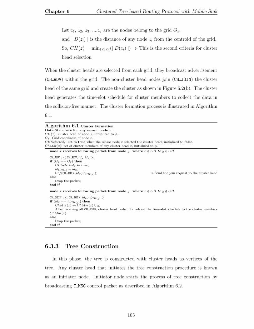
Chapter 6 Clustered Tree based Routing Protocol with Mobile Sink
Let z1, z2, z3, ....zj are the nodes belong to the grid Gz.
and | D(zi) | is the distance of any node zi from the centroid of the grid.
So, CH(z) = min1≤i≤j(| D(zi) |) . This is the second criteria for cluster
head selection
When the cluster heads are selected from each grid, they broadcast advertisement
(CH ADV) within the grid. The non-cluster head nodes join (CH JOIN) the cluster
head of the same grid and create the cluster as shown in Figure 6.2(b). The cluster
head generates the time-slot schedule for cluster members to collect the data in
the collision-free manner. The cluster formation process is illustrated in Algorithm
6.1.
Algorithm 6.1 Cluster FormationData Structure for any sensor node x :CH(x): cluster head of node x, initialized to φ.Gx: Grid coordinate of node x.CHSelectedx: set to true when the sensor node x selected the cluster head, initialized to false.ChMbr(x): set of cluster members of any cluster head x, initialized to φ.
node x receives following packet from node y: where x /∈ CH & y ∈ CH
CH ADV : < CH ADV, idy , Gy >;if (Gx == Gy) then
CHSelectedx ← true;idCH(x) = idy ;l rf(CH JOIN, idx, idCH(x)); . Send the join request to the cluster head
elseDrop the packet;
end if
node x receives following packet from node y: where x ∈ CH & y /∈ CH
CH JOIN : < CH JOIN, idy , idCH(y) >if (idx == idCH(y)) then
ChMbr(x)← ChMbr(x) ∪ y;After receiving all CH JOIN, cluster head node x broadcast the time-slot schedule to the cluster members
ChMbr(x).else
Drop the packet;end if
6.3.3 Tree Construction
In this phase, the tree is constructed with cluster heads as vertices of the
tree. Any cluster head that initiates the tree construction procedure is known
as an initiator node. Initiator node starts the process of tree construction by
broadcasting T MSG control packet as described in Algorithm 6.2.
105

Chapter 6 Clustered Tree based Routing Protocol with Mobile Sink
Algorithm 6.2 Tree ConstructionData Structure for any sensor node x :Children(x) : children set of node x, initialized to φ.Parent(x) : parent of node x, initialized to φ.IsCHx : it is true if any node x is a cluster head.Parent Selectedx : set to true when the sensor node x selects its parent, initialized to false.T MSGSentx : set to true when the sensor node x sends T MSG packet, initialized to false.
node x receives following packets from node y:
T MSG : < T MSG, idy , Parent(y) >if (IsCHx == true) then
if (idx == Parent(y)) thenChildren(x) � Children(x) ∪ {idy};
else if (Parent Selectedx == false) thenParent(x) � idy ;Parent Selectedx � true;if ((T MSGSentx == false)) then
T MSGSentx � true;l rb(T MSG, idx, Parent(x)); . Broadcast T MSG packet
elseDrop the packet;
end ifend if
elseDrop the packet;
end if
When the cluster heads of the different grids receive the T MSG they perform
following operations:
• If the recipient is the cluster head, it checks the sender’s parent id and if it is
the same as the receiver node id, then include the sender id in the children
list Children(x).
• If it has not selected any parent, then select sender node as its parent.
• If T MSGSent is false, then broadcast T MSG packet with modified
parameter to the network.
In this way, the tree is constructed with the parent and child nodes as shown in
Figure 6.3(a). The purpose of the tree formation is to make sure that the network
is connected. The link between the parent and child node would be bidirectional.
6.3.4 Mobile Sink Management
The sink follows the random waypoint mobility model. It is required to manage
the sink mobility. The sink moves from one location to another and collects the
data. In the new position, sink waits to gather the data, this duration is called
106

Chapter 6 Clustered Tree based Routing Protocol with Mobile Sink
(a) Initial view of Tree Construction. (b) Mobile sink management through thegateway node.
Figure 6.3: Tree Construction and Mobile Sink Management.
pause time (δ). One of the closest cluster head elected as a gateway node by the
sink. The gateway node informs the rest of the cluster head through the tree. The
cluster head nodes make the link towards the gateway node for transmitting the
data as demonstrated in Figure 6.3(b). The detailed packet communication for
sink management is illustrated in Algorithm 6.3. When the mobile sink reaches
to the new position, it broadcasts a Beacon packet. The Beacon packet consists
of sink id. The cluster head that receives the beacon should reply the sink with
BeaconRelay packet. The BeaconReply packet consists of its id and the sink id.
When the sink receives the first BeaconReply packet, it selects that sender cluster
head as the gateway and transmits a Gateway packet. The gateway packet consists
of sink id and selected gateway node id. When the selected gateway node receives
the packet, it selects the next node as the sink to transmit the data and broadcasts
the acknowledgment (ACK) packet. The ACK packet consists of the sender id and
gateway node id. The recipient cluster head performs the following operations:
• Checks if the ACK packet sender is a parent or a child, then
• Checks if the ACK packet is not for the previous gateway node, then
• Selects the gateway node as newly selected gateway node and selects
next node as sender node id.
• Forwards the ACK with its id and gateway node id.
107

Chapter 6 Clustered Tree based Routing Protocol with Mobile Sink
In this way, each cluster head selects the next cluster head to transmit the data.
When the sink moves from its current position, it sends a STOP signal to the
gateway node. The gateway node forwards the STOP signal in the network. So
that all the cluster heads halt the transmission until the sink selects the new
gateway. It increases the data delivery ratio and decreases the data loss.
Algorithm 6.3 Mobile Sink ManagementData Structure for any sensor node x and sink:Gatewaysink : gateway node selected by the sink.Gateway selected: set to true once the sink chooses the gateway node, initialized to false.next nodex: the cluster head x selects the next cluster head for data transmission.SendDatax : set to true once the cluster head chooses the next nodex for data transmission, initialized to false.IsCHx : it is true if any node x is a cluster head.Gatewayx : gateway node selected by the node x.
node x receives following packets from the sink:
Beacon: < Beacon, idsink >if (IsCH) then
l rf(BeaconReply, idx, idsink); . Unicast the BeaconReply packet to the sink.end if
the sink receives following packets from cluster head y:
BeaconReply: < BeaconReply, idy, idsink >if (Gateway selected == false) then
Gatewaysink � idy ;Gateway selected � true;l rf(Gateway, idsink , Gatewaysink); . the sink unicasts the Gateway packet to the selected gateway node.
elseDrop the packet;
end if
cluster head node x receives following packets from the sink:
Gateway: < Gateway, idsink , Gatewaysink >if (idx == Gatewaysink) then
next nodex � idsink ;l rb(ACK, idx, Gatewaysink); . Boradcast the ACK packet.
elseDrop the packet;
end if
cluster head node x receives following packets from node y:
ACK: < ACK, idy , Gatewaysink >if (IsCH &&((idy ∈ Parent(x)) || (idy ∈ Children(x)))) then
if (Gatewayx 6= Gatewaysink) thenGatewayx � Gatewaysink ;SendDatax � true;next nodex � idy ;l rb(ACK, idx, Gatewaysink); . Boradcast the ACK packet.
end ifelse
Drop the packet;end if
6.3.5 Data Transmission
The cluster member sends their data to the cluster head and switch to sleep
mode until the next time-slot. The cluster head aggregates the data. If the
108

Chapter 6 Clustered Tree based Routing Protocol with Mobile Sink
SendData flag is true, then it can immediately start the data transmission to the
next cluster head (next node). Once the data packet reaches the gateway node,
it forwards the data to the sink. The detail description is illustrated in Algorithm
6.4.
Algorithm 6.4 Data TransmissionData Structure for any sensor node x :SendDatax : set to true once the relay node chooses the next nodex for data transmission, initialized to false.Send Data(x) : node x add the pair of id and sec no after receiving the DATA packet, initialized to φ.
node x will receive following packet from node y ∈ Nbr(x):
DATA : < DATA, idsource, sec nosource, Nextnodey >if (idx == Nextnodey) then
if (< idsource, sec nosource > /∈ Send Date(x)) thenSend Data(x) � Send Data(x) ∪ {idsource, sec nosource};if (SendDatax == true) then
l rf(DATA, idsource, sec nosource, next nodex); . Forward the DATA packet to the next node.end if
end ifelse
Drop the packet;end if
The recipient node performs the following operations:
• Checks if the receiver node is the same as the next node id, then
• Checks if it receives the new data, then
• Adds the source id and sequence number in the Send Data table and
• If the SendData flag is true, then forwards the data to its next cluster head.
6.3.6 Load Balancing
In the proposed protocol, every node can compute their residual energy. When
the cluster head’s energy level reaches below to the threshold value, the protocol
initiates the cluster head selection process. Once the new cluster head is selected,
it builds the cluster and begins the tree construction process. In this way, the
protocol balances the load among the sensor nodes, and it helps to increase the
lifetime of the network.
109

Chapter 6 Clustered Tree based Routing Protocol with Mobile Sink
6.4 Simulation Results
To validate and compare the proposed protocol with the TEDD and DTRP
in terms of performance metrics mentioned in the Chapter 2. An extensive set of
experiments have been done using the Castalia (v3.2) simulator and based on the
parameters shown in Table 6.1.
Parameter Name Value
Network area 500 × 500 meter2
Number of sensor nodes 200Data packet size 512 bytesControl packet size 32 bytesInitial energy 1Jδ 5 secSink speed (5, 10, 15, 20, 25, 30) m/secMobility Model Random WaypointEelec 50 nJ/bitεfs 10 pJ/bit/m2
εmp 0.0013 pJ/bit/m4
d0 87 metersEproc 5 nJ/bitElow 0.2 nJ/secondSimulation time 400 secMAC protocol TMAC
Table 6.1: Simulation Parameters.
6.4.1 Average Control Packet Overhead
Figure 6.4 illustrated the average energy consumption of control packet with
varying sink speed. The sensor node transmits the control packets to construct the
cluster and tree and manage the sink mobility. In TEDD, DTRP and proposed
protocol, the tree structure is independent of the sink mobility. However, when
the role of a node changes from the relay to non-relay or non-relay to relay, in
TEDD the entire tree has to construct once again. In case of DTRP, only two hop
neighbors are affected. In the proposed protocol, the control packet overhead for
sink management and tree reconstruction are less than the existing protocols due
to fewer cluster heads.
110

Chapter 6 Clustered Tree based Routing Protocol with Mobile Sink
5 10 15 20 25 30
0.05
0.1
0.15
0.2
0.25
Sink speed (m/s)
Ave
rag
e c
on
tro
l p
acke
ts o
ve
rhe
ad
(J)
TEDD
DTRP
Proposed
Figure 6.4: Control Packet Overhead
6.4.2 Average Energy Consumption
The average energy consumption of the nodes in the network for data and
control packet is shown in the Figure 6.5. TEDD and DTRP do not aggregate
the data. However, in the proposed protocol, the cluster head aggregates and
transmits the data to the sink through the tree. It reduces the total data packet
received by the sink. Therefore, the average energy consumption is less in the
proposed protocol.
5 10 15 20 25 30
0.2
0.3
0.4
0.5
Sink speed (m/s)
Ave
rag
e e
ne
rgy c
on
su
mp
tio
n (
J)
TEDD
DTRP
Proposed
Figure 6.5: Average Energy Consumption
111

Chapter 6 Clustered Tree based Routing Protocol with Mobile Sink
6.4.3 Average End-to-End Latency
It is the time duration between data generation and successful reception at the
sink. Figure 6.6 shows the average end-to-end latency with various sink speeds.
The proposed protocol takes less cost and time to manage the mobility of the sink
and tree reconstruction than TEDD and DTRP. It is because of the tree formation
using cluster head rather relay nodes.
5 10 15 20 25 30
0.005
0.01
0.015
0.02
Sink Speed (m/s)
Ave
rag
e d
ata
de
live
ry la
ten
cy (
s)
TEDD
DTRP
Proposed
Figure 6.6: Average End-to-End Latency
5 10 15 20 25 30
60
70
80
90
100
Sink speed (m/s)
Da
ta d
eliv
ery
ra
tio
(%
)
TEDD
DTRP
Proposed
Figure 6.7: Packet Delivery Ratio
112

Chapter 6 Clustered Tree based Routing Protocol with Mobile Sink
6.4.4 Packet Delivery Ratio
Figure 6.7 presents the data delivery ratio with respect to different sink speeds.
Data delivery ratio shows the reliability of the network. It can be measured by
the ratio between the data received by the sink and sent by the sensor nodes.
The sink mobility increases the link failure, which causes data loss. The proposed
protocol efficiently manages the route than TEDD and DTRP. Furthermore, in the
proposed protocol, the total data transmissions are less than TEDD and DTRP.
It increases the delivery ratio of the proposed protocol.
6.4.5 Network Lifetime
The network lifetime of the proposed scheme is greater than the TEDD and
DTRP as shown in Figure 6.8. It is due to the less control packet overhead and
aggregated data. The proposed protocol also balances the load among the sensor
nodes, which makes the proposed protocol more energy-efficient and leads to the
increased network lifetime.
50 100 150 200 250 300 350 400
120
140
160
180
200
Simulation time (s)
Nu
mb
er
of
no
de
s a
live
TEDD
DTRP
Proposed
Figure 6.8: Network Lifetime
113

Chapter 6 Clustered Tree based Routing Protocol with Mobile Sink
6.5 Summary
In this chapter, a clustered tree based routing protocol (CTRP) has been
proposed to address the flaws of TEDD and DTRP. CTRP efficiently send the
data to sink and minimize the battery power consumption of sensor nodes. A
cluster is formed in each grid, and a cluster head is selected. CTRP creates a tree
using these cluster heads. CTRP can manage the sink mobility without affecting
the tree structure. It balances the load among the sensor nodes which increases
the network lifetime. Simulation results showed that CTRP outperformed TEDD
and DTRP in terms of energy consumption, end-to-end latency, data delivery ratio
and network lifetime.
114

7
Rendezvous based Routing Protocol
with Mobile Sink
Introduction
System Model
The Proposed Protocol
Simulation Results
Summary

Chapter 7
Rendezvous based RoutingProtocol with Mobile Sink
7.1 Introduction
The network with mobile sink implicitly balances the load among the sensor
nodes and reduces the chance of hotspots [103]. It can help to achieve the uniform
energy consumption and prolong the lifetime. On the other hand, some problems
are associated with the mobile sink. The mobile sink frequently required to send its
current position information across the network. This process causes a significant
energy consumption overhead. Addition to that, the mobile sink makes the sensor
network dynamic in nature. Hence, it is not feasible to find the routing path prior
to its requirement. Generally, in the reactive routing, the end-to-end latency is
high, which can compromise the requirement of fresh data. In the event-based
application, the validity of the sensor data depends on its freshness. The delayed
data is of no use. So the primary requirement of the event-based application
is to reduce the end-to-end latency. Latency may be affected by many factors
like availability of routing path, known mobile sink location, the existence of
non-interference paths, etc.
It has been observed that the rendezvous based approaches are suitable for
the time-sensitive applications. They are capable of reducing the latency. In the
mobile sink environment, the source node has to wait until it gets the routing
path to transmit the data. In rendezvous based routing some predefined area
is specified, where the source node can communicate. In some approaches like
116

Chapter 7 Rendezvous based Routing Protocol with Mobile Sink
Line Based Data Dissemination (LBDD) [75] and Grid-based energy efficient
routing [74], source node can transmit the data to the rendezvous region, and
the rendezvous nodes can further forward the data to the sink. Whereas, in
the approaches like Railroad [76] and Ring routing [77], source node can retrieve
the current position of the sink from the rendezvous region and transmit the
data directly to the sink through intermediate nodes using geographical based
approaches [44, 45]. In the first types of approaches, the end-to-end latency is
very less, but it compromises the energy-efficiency. Whereas the second types
of approaches are energy-efficient, but it compromises the latency. It motivated
to propose rendezvous based routing protocol, which can be energy-efficient and
takes less time to deliver the sensed data.
In this chapter, a Rendezvous based Routing Protocol (RRP) is proposed,
which addresses the requirement of energy-efficiency and less end-to-end latency.
In RRP, a virtual cross area is created in the middle of the network. It is
called rendezvous region, and the nodes belong to this region are called backbone
nodes. A tree is formed within the rendezvous region, and each sensor node can
communicate with the rendezvous region. In RRP, two methods are proposed
for the data transmission. In the first method, the source node transmits the
data to the sink through the rendezvous region. In the second method, source
node retrieves the position of the sink and transmits the data to the sink using
geographical based approach [44]. The system model is defined in Section 7.2, In
Section 7.3 the description of the proposed protocol is presented. The simulation
result and analysis are discussed in Section 7.4 and finally, the proposed protocol
is summarized in Section 7.5.
7.2 System Model
7.2.1 Network Model
The network consists of n number of sensor nodes and a sink. The sensor
nodes are static, and a sink is moving within the network with the speed varying
from 5 to 30meter/second. A pause time (δ) for the sink is considered to collect
117

Chapter 7 Rendezvous based Routing Protocol with Mobile Sink
the data. A virtual horizontal and vertical region of width w is considered. It
resides in the middle portion of the network having a center position (u, v). This
region has four parts such as: (i) horizontal left hl, (ii) horizontal right hr, (iii)
vertical up vu and (iv) vertical bottom vb as shown in Figure 7.2(a). If the sensor
node is detected any event, then it should report to the sink. The energy model
for the sensor node is the same as stated in Chapter 2. Besides, the assumptions
are taken in Chapter 4 the additional assumptions are considered. The Random
Waypoint mobility model has been considered for the sink mobility. The sensor
node can find their location information, and the node can vary their transmission
range up to the maximum range R. Each node can calculate their residual energy.
7.3 The Proposed Protocol
The proposed protocol is a rendezvous based routing protocol. In this, a virtual
cross area is created of width w, in the middle region of the network. These cross
area acts as a rendezvous region for sensor node communication. The nodes in
rendezvous area are called backbone node. A tree has been created in the cross
area. This tree involves only a few backbone nodes, and it is created such a way
that the boundaries can be covered. The tree nodes are responsible to forward
the information from the source to the sink or from the sink to the source. The
proposed protocol consists of various phases such as neighbor discovery, cross area
formation, tree construction, sensor node region discovery and data transmission.
7.3.1 Neighbor Discovery
In this phase, each sensor node finds the neighbors information as discussed in
the Algorithm 7.1. The initiator node broadcasts a control packet NBR DET, which
contains the node id, residual energy and the location information. The neighbor
node that receives the NBR DET packet will maintain a table called NbrTable. The
NbrTable consists of node id of the sender, its residual energy, and location. If
the sender node id is already in the NbrTable, then the packet is dropped by
the receiver node. The receiver node creates and broadcasts the NBR DET control
118

Chapter 7 Rendezvous based Routing Protocol with Mobile Sink
packet if it did not broadcast before. At the end of the neighbor discovery phase,
each node has the one-hop neighbor list and corresponding information.
Algorithm 7.1 Neighbor DiscoveryData Structure for any sensor node x :Nbr(x): neighbor set of node x, initialized to φ.NbrTable(x): neighbor table of node x, initialized to φ.Erx: residual energy of any node x.NbrDETSentx : set to true when the sensor node x sends NBR DET packet, initialized to false.
node x receives following packet from node y:
NBR DET :< NBR DET, idy , Ery, Locy >if (y /∈ Nbr(x)) then
Nbr(x) � Nbr(x) ∪ {y};Update NbrTable(x) with < idy , Ery, Locy >;if (NbrDETSentx == false) then
NbrDETSentx � true;l rb(NBR DET, idx, Erx, Locx); . Broadcast NBR DET packet
elseDrop the packet;
end ifelse
Drop the packet;end if
7.3.2 Cross Area Formation
The proposed protocol divides the sensor field into equal parts of a vertical,
and a horizontal stripe called cross area as shown in Figure 7.1(a).
Sensor Nodes
(a) Initial view of Rendezvous region.
Backbone Nodes Sensor Nodes
(b) Initial view of Backbone nodes.
Figure 7.1: Rendezvous region and Backbone nodes.
The node belongs to the cross area are called the backbone nodes. Let’s
consider w is the width of the strip and maximum network area is (xmax, ymax).
119

Chapter 7 Rendezvous based Routing Protocol with Mobile Sink
So, wx and wy, the horizontal and vertical ranges of the backbone are defined as
shown in Equation (7.1).
wx =
(
xmax − w
2
)
to
(
xmax + w
2
)
;wy =
(
ymax − w
2
)
to
(
ymax + w
2
)
; (7.1)
If any sensor node belongs to the range of wx and wy, it can be labeled as a
backbone node. In the protocol, the Cross area used as a rendezvous region. This
region works as a communication point for the sensor nodes. The rendezvous
region and backbone node in the network are shown in Figure 7.1.
7.3.3 Tree Construction
The tree construction is performed inside the rendezvous region. The protocol
allows only some of the backbone nodes to take part in the tree construction. The
boundary nodes of the four sections of rendezvous region hr, hl, vu, vb as shown in
Figure 7.2(a), start the process of tree construction. Each node has the neighbor
information that includes id, residual energy and the location. The boundary node
selects one of its neighbor using the following criteria:
1. The node should be a backbone node,
Let BBx is true if any node x labeled as backbone node,
Nbr(x) is a set of neighbor node of x and
z is a sensor node;
if (z ∈ Nbr(x) && BBz == true) then
z can be chosen by x in tree construction . First criteria for node
selection.
end if
2. the residual energy of the backbone node should be greater than the
threshold value,
Er(z) is the residual energy of any node z ∈ Nbr(x), then
Er(z) ≥ Ethreshold . Second criteria for node selection.
120

Chapter 7 Rendezvous based Routing Protocol with Mobile Sink
3. and the sensor node should be closer to the centroid of the network.
Let z1, z2, z3, ....zj are the nodes belong to the backbone and Nbr(x) and
| D(zi) | is the distance of any node zi form the centroid of the network
So, z = min1≤i≤j(| D(zi) |) . Third criteria for node selection.
After selecting one of the neighbor nodes, the boundary node transmits the control
packet to the selected node for tree construction. The receiver node makes the
sender node as the parent and selects the next neighbor node closest to the
centroid. This process repeats until the packet initiated by the boundary node
reaches the centroid of the network as shown in Figure 7.2(b).
vu
hr
Sensor NodesBackbone Nodes
hl
vb
(a) Rendezvous region with the boundary hr,hl, vu and vl.
vu
hr
vb
hl
(b) Final view of tree construction.
Figure 7.2: Rendezvous region and Tree within the rendezvous region.
7.3.4 Sensor Node Region Discovery
After the tree construction, the sensor node can communicate with the
backbone-tree nodes. In this process, the sensor node is required to find out the
region in which it belongs. So, the sensor node can find the shortest destination
to communicate with the rendezvous region. The network is virtually divided into
octants as illustrated in Figure 7.3(a). The sensor node follows the Algorithm 7.2
with the location information of itself and location of the centroid of the network
to get the shortest destination.
121

Chapter 7 Rendezvous based Routing Protocol with Mobile Sink
vu
hr
vb
hl
Backbone Nodes Sensor NodesSink
VII
VIII
VI
V
IV
III II
I
(a) Virtually divided octants region.
Gat"way
#ourc
$ vu
hr
vb
hl
(b) Gateway node selection.
Figure 7.3: Sensor node region discovery and Gateway node selection.
The sensor nodes can calculate the octant in which they belong using their
location information (x,y). For example, if the nodes belonging to 1st and 8th
octant, it will communicate from hr with destination location (x, v). Similarly, 2nd
and 3rd octant sensor node can communicate from vu with destination location
(u, y) and so on, where (u, v) are the center location of the network.
7.3.5 Data Transmission
The sensor node monitors the environment and accordingly generates the data.
In the proposed protocol, the source nodes can send the data to the sink whenever
they required. Two different methods are considered to send the data to the
mobile sink. In the first method, the source node transmits the data to the closest
backbone-tree node. The backbone-tree node forwards the data to the sink. In
the second method, the source node retrieves the sink location from the nearest
backbone-tree node and transmits the data directly to the sink by using the sink
location. Both the methods are described in the following sections.
122

Chapter 7 Rendezvous based Routing Protocol with Mobile Sink
Algorithm 7.2 Node Region Discoveryvariables : θ = 0; α = 0;(u, v): center location of the network.(x, y): any sensor node location in the network.
Let π = 1800;C ←− (u, v); . C is the center of the network.for any node z in the network with location(x, y)Let new coordinates (A,B)←− (x− u, y − v); . evaluate (A,B) corresponding to the center C.
Calculate θ = tan−1∣
∣
∣
BA
∣
∣
∣
if (A>0&&B>0) thenα ←− θ . node with location (x, y) is in 1st quadrant.if (α lies between 0 to π/4) then
Node with location(x, y) belongs to 1st octant and node can communicate from hr with destinationlocation (x, v).
else if (α lies between π/4 to π/2) thenNode with location (x, y) belongs to 2nd octant and node can communicate from vu with destination
location (u, y).end if
end ifif (A<0&&B>0) then
α ←− π − θ . node with location (x, y) is in 2nd quadrant.if (α lies between π/2 to 3π/4) then
Node with location(x, y) belongs to 3rd octant and node can communicate from vu with destinationlocation (u, y).
else if (α lies between 3π/4 to π) thenNode with location (x, y) belongs to 4th octant and node can communicate from hl with destination
location (x, v).end if
end ifif (A<0&&B<0) then
α ←− π + θ . node with location (x, y) is in 2nd quadrant.if (α lies between π to 5π/4) then
Node with location(x, y) belongs to 5th octant and node can communicate from hl with destinationlocation (x, v).
else if (α lies between 5π/4 to 3π/2) thenNode with location (x, y) belongs to 6th octant and node can communicate from vb with destination
location (u, y).end if
end ifif (A>0&&B<0) then
α ←− 2π − θ . node with location (x, y) is in 2nd quadrant.if (α lies between 3π/2 to 7π/4) then
Node with location(x, y) belongs to 7th octant and node can communicate from vb with destinationlocation (u, y).
else if (α lies between 7π/4 to 2π) thenNode with location (x, y) belongs to 8th octant and node can communicate from hr with destination
location (x, v).end if
end if
7.3.6 Proposed Method 1
Mobile Sink Management
The sink is moving within the network using the random waypoint mobility
model. The mobile sink always moves into the network and pause for a certain
time (δ) to collect the data.
When the sink reaches to a new position, it selects a gateway node for data
collection. The gateway node forwards the ACK packet towards the backbone node
123
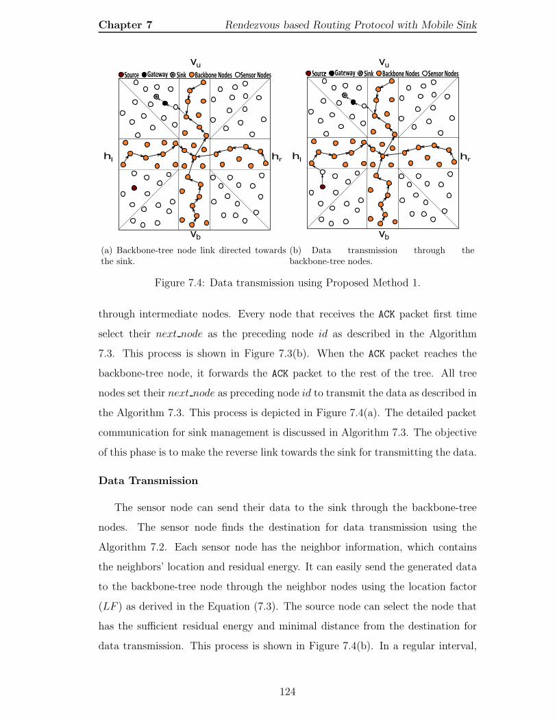
Chapter 7 Rendezvous based Routing Protocol with Mobile Sink
vu
hr
vb
hl
Gat%way
&ourc
'
(a) Backbone-tree node link directed towardsthe sink.
Gat(way
)ourc
* vu
hr
vb
hl
(b) Data transmission through thebackbone-tree nodes.
Figure 7.4: Data transmission using Proposed Method 1.
through intermediate nodes. Every node that receives the ACK packet first time
select their next node as the preceding node id as described in the Algorithm
7.3. This process is shown in Figure 7.3(b). When the ACK packet reaches the
backbone-tree node, it forwards the ACK packet to the rest of the tree. All tree
nodes set their next node as preceding node id to transmit the data as described in
the Algorithm 7.3. This process is depicted in Figure 7.4(a). The detailed packet
communication for sink management is discussed in Algorithm 7.3. The objective
of this phase is to make the reverse link towards the sink for transmitting the data.
Data Transmission
The sensor node can send their data to the sink through the backbone-tree
nodes. The sensor node finds the destination for data transmission using the
Algorithm 7.2. Each sensor node has the neighbor information, which contains
the neighbors’ location and residual energy. It can easily send the generated data
to the backbone-tree node through the neighbor nodes using the location factor
(LF ) as derived in the Equation (7.3). The source node can select the node that
has the sufficient residual energy and minimal distance from the destination for
data transmission. This process is shown in Figure 7.4(b). In a regular interval,
124

Chapter 7 Rendezvous based Routing Protocol with Mobile Sink
Algorithm 7.3 Mobile Sink Management (Proposed Method 1)Data Structure for any sensor node x and sink:Gatewaysink : gateway node selected by the sink.Gateway selected: set to true once the sink chooses the gateway node, initialized to false.next nodex: the cluster head x selects the next cluster head for data transmissionx.SendDatax : set to true once the cluster head chooses the next nodex for data transmission, initialized to false.BBx : is true if any node x labeled as the backbone node;Gatewayx : gateway node selected by the node x.
Node x receives following packets from the sink:
Beacon: < Beacon, idsink >l rf(BeaconReply, idx, idsink); . Unicast the BeaconReply packet to the sink.
the sink receives following packets from y:
BeaconReply: < BeaconReply, idy, idsink >if (Gateway selected == false) then
Gatewaysink � idy ;Gateway selected � true;l rf(Gateway, idsink , Gatewaysink); . the sink unicasts the Gateway packet to the selected gateway node.
elseDrop the packet;
end if
node x receives following packets from the sink:
Gateway: < Gateway, idsink , Gatewaysink >if (idx == Gatewaysink) then
next nodex � idsink ;As described in the Algorithm 7.2 the gateway node chooses the backbone and destination location.The node forwards the ACK packet to the node z closest to the destination using the Equation (7.3).l rf(ACK, idx, idz , Gatewaysink); . Forwards the ACK packet.
elseDrop the packet;
end if
node x receives following packets from the node y ∈ Nbr(x):
ACK: < ACK, idy , idz , Gatewaysink >if (idx == idz) then
if (Gatewayx 6= Gatewaysink) thenGatewayx � Gatewaysink ;SendDatax � true;next nodex � idy ;if (BBx == true&&Parentx == true) then
Choose the node z as parent and child id;else
Choose the node z closest to the destination using the Equation (7.3).end ifl rf(ACK, idx, idz , Gatewaysink); . Forwards the ACK packet in the tree.
elseDrop the packet;
end ifelse
Drop the packet;end if
each node broadcast their residual energy to update the neighbor information.
Let node i required to select the nodes from its neighbors. Nbr(i) is the set of
neighbors of node i. LF (i) is the set of location factors of each member of Nbr(i).
Erk is the residual energy of node k ∈ Nbr(i). (xk, yk) is the location information
of node k ∈ Nbr(i) and Dk is the Euclidean distance from the destination.
Let, Ermax = maxk∈Nbr(i) Er
125

Chapter 7 Rendezvous based Routing Protocol with Mobile Sink
then for kth neighbor LFk can be computed as
LFk = Erk ×1
Dk
=ErkDk
∀k : k ∈ Nbr(i) (7.2)
where,
Erk = ErkErmax
Dk =√
(xdest − xk)2 + (ydest − yk)2
and,
next nodei = max (LF (i)) (7.3)
where, next nodei is the sensor node selected by the node i.
7.3.7 Proposed Method 2
Mobile Sink Management
In the second method of rendezvous based routing protocol, the sink node
informs its position to the backbone-tree nodes. They have the latest location
information of the sink as shown in Figure 7.5(a).
vu
hr
vb
hl
Sourc+
(a) Sink location recovery.
Sourc, vu
hr
vb
hl
(b) Data transmission.
Figure 7.5: Data transmission using Proposed Method 2.
When a sink node moves to a new position, it broadcast a Beacon packet to get
the neighbor information. The sink selects one of its neighbor nodes to forward
126

Chapter 7 Rendezvous based Routing Protocol with Mobile Sink
the location information. Sink refers the Algorithm 7.2 and Equation (7.3) to
select the forwarding node. The forwarding node again relays the sink’s location
to its neighbor using the same technique. When location information reaches the
backbone-tree node, it disseminates the location information into the tree. The
communication detail on the sink management is discussed in Algorithm 7.4.
Algorithm 7.4 Mobile Sink Management (Proposed Method 2)Data Structure for any sensor node x and sink:Sink Locx : any node x stores the sink location information.BBx : is true if any node x labeled as the backbone node, initialized as false.Locsink : the location of the sink.
Beacon: < Beacon, idsink >l rf(BeaconReply, idx, Erx, idsink); . Unicast the BeaconReply packet to the sink.
As described in the Algorithm 7.2 the sink node chooses the backbone to send its location.The sink node forwards the Location packet to the node z using the Equation (7.3).l rf(Location, idsink , Locsink , next nodez); . Unicast the Location packet to the selected node z.Node x receives following packets from the sink or any node y:
Location : < Location, idy , Locsink, next nodey >if (idx == next nodey) then
if (Sink Locx 6= Locsink) thenSink Locx � Locsink ;if (BBx == true&&Parent(x) == true) then
Choose the node z as parent and child id;else
Choose the node z closest to the destination using the Equation (7.3).end ifl rf(Location, idx, Locsink , next nodez); . Unicast the Location packet to the selected node z.
elseDrop the packet;
end ifelse
Drop the packet;end if
Sink Location Recovery and Data Transmission
To transmit the data source node needs to find the sink location. It can get
the sink location from the backbone-tree nodes. For finding the sink location the
source, the node makes a request to the backbone-tree node by sending a Loc Req
packet. When the backbone-tree node receives the request, it replies with the sink
location as shown in Figure 7.5(a). The sink location recovery process is discussed
in the Algorithm 7.5.
After getting the sink location, the source node transmits the data to sink
through the neighbor nodes. It selects one of the neighbor nodes having sufficient
residual energy and minimum distance from the sink as mentioned in Equation
(7.3). When the neighbor node receives the data, it selects another node from its
127

Chapter 7 Rendezvous based Routing Protocol with Mobile Sink
Algorithm 7.5 Sink Location Recovery (Proposed Method 2)Data Structure for any sensor node x:Sink Locx: any node x stores the sink location information.BBx : is true if any node x labeled as the backbone node;Locsink : the location of the sink.next nodex : any sensor node x selects the next node for packet transmission .reverse linkx : any sensor node x select the sender for sending sink location
As described in the Algorithm 7.2 the source node chooses the destination to send the location request.The source node forwards the Loc Req packet to next node using the Equation (7.3).l rf(Loc Req, idx, next nodex); . Unicast the Location packet to the selected next node.
Node x receives following packets from any node y ∈ Nbr(x):Loc Req : < Loc Req, idy , next nodey >if (idx == next nodey) then
reverse linkx � idy ;if (BBx == true&&Parent(x) == true) then
l rf(Loc Reply, idx, Locsink, reverse linkx); . Reply the sink location to the requested node.else
The node selects the next node using the Equation (7.3).l rf(Loc Req, idx, next nodex); . Unicast the Loc Req packet to the next node.
end ifelse
Drop the packet;end if
Node x receives following packets from any node y ∈ Nbr(x):Loc Reply : < Loc Reply, idy , Locsink , reverse linky >if (idx == reverse linky) then
if (idx == idsource) thenSink Locx � Locsink ;
elsel rf(Loc Reply, idx, Locsink, reverse linkx); . Unicast the Location packet to the requested node.
end ifelse
Drop the packet;end if
neighbor list using the technique as mentioned above. Figure 7.5(b) illustrated
the data transmission from the source to the sink through intermediate nodes.
7.4 Simulation Results
Through the simulation, the proposed protocols performance has been analyzed
and compared with the existing protocols such as Line Based Data Dissemination
(LBDD) [75], Railroad [76], and Ring routing [77]. Each experiment has been
performed with the varying sink speed from 5meter/second to 30meter/second.
The impact of the sink speed in energy consumption, end-to-end latency, and data
delivery ratio has been observed. An extensive set of simulation is performed based
on the parameter illustrated in Table 7.1 using the Castalia (v3.2) simulator.
128

Chapter 7 Rendezvous based Routing Protocol with Mobile Sink
Parameter Name Value
Network area 500 × 500 meter2
Number of sensor nodes 200Data packet size 512 bytesControl packet size 32 bytesInitial energy 1Jδ 5 secSink speed (5, 10, 15, 20, 25, 30) m/secMobility Model Random WaypointEelec 50 nJ/bitεfs 10 pJ/bit/m2
εmp 0.0013 pJ/bit/m4
d0 87 metersElow 0.2 nJ/secondSimulation time 600 secMAC protocol TMAC
Table 7.1: Simulation Parameters.
7.4.1 Average Control Packet Overhead
The sensor node transmits the control packets to construct the rendezvous
region and manage the sink mobility. The average energy consumption of control
packet with varying sink speed for various protocols is illustrated in Figure 7.6.
As the result shown in the graph, the control packet overhead is very less in the
Proposed Method 2 as compared to the other protocols.
In LBDD, an inline-node stores the data from the source node. When that
inline-node receives the query, it sends the data to the sink. The sink’s query has
been flooded into the rendezvous region, which causes an increased control packet
overhead. In the railroad protocol, the rail construction and station formation
is the one-time process. However, the process of metadata storage at station
and retrieval of the sink location from the station requires the control packet
exchange. In ring routing, all the ring nodes store the location of the sink. So
the retrieval of the sink location is easier. However, as the network operation
progresses, it requires the exchange of control packets to repair the ring. So
the ring length increases, and as a result, the distance from the source or the
sink causes more energy consumption. The Proposed Method 1 only needs to
maintain the tree within the rendezvous region to transmit the data. The control
129
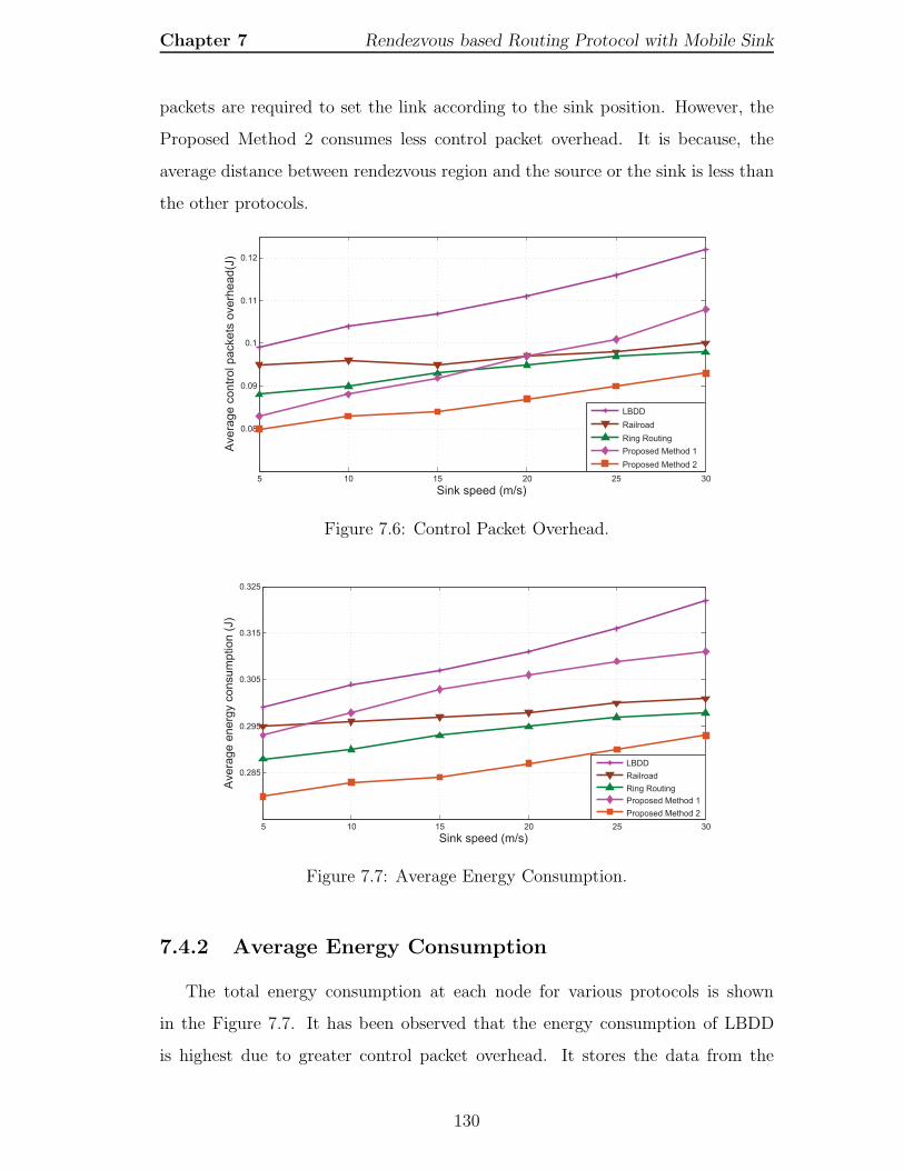
Chapter 7 Rendezvous based Routing Protocol with Mobile Sink
packets are required to set the link according to the sink position. However, the
Proposed Method 2 consumes less control packet overhead. It is because, the
average distance between rendezvous region and the source or the sink is less than
the other protocols.
5 10 15 20 25 30
0.08
0.09
0.1
0.11
0.12
Sink speed (m/s)
Ave
rag
e c
on
tro
l p
acke
ts o
ve
rhe
ad
(J)
LBDD
Railroad
Ring Routing
Proposed Method 1
Proposed Method 2
Figure 7.6: Control Packet Overhead.
5 10 15 20 25 30
0.285
0.295
0.305
0.315
0.325
Sink speed (m/s)
Ave
rag
e e
ne
rgy c
on
su
mp
tio
n (
J)
LBDD
Railroad
Ring Routing
Proposed Method 1
Proposed Method 2
Figure 7.7: Average Energy Consumption.
7.4.2 Average Energy Consumption
The total energy consumption at each node for various protocols is shown
in the Figure 7.7. It has been observed that the energy consumption of LBDD
is highest due to greater control packet overhead. It stores the data from the
130

Chapter 7 Rendezvous based Routing Protocol with Mobile Sink
source node and floods the sink’s query in the rendezvous region. The energy
consumption of the LBDD grows monotonically as the sink speed increases. The
Proposed Method 1 does not require sink location, but the average path length is
higher than Railroad, Ring routing and Proposed Method 2. So the overall energy
consumption is more and increases according to the sink speed. In the Proposed
Method 2, the average distance between source and the sink is almost the same as
the Railroad and Ring routing. However, due to the less control packet overhead,
the Proposed Method 2 outperforms the existing protocols.
7.4.3 Average End-to-End Latency
Figure 7.8 presents the average end-to-end latency of different protocols with
various sink speeds. It depends on the time duration to find the sink’s location
and propagate the data to the sink. The Proposed Method 1 instantly transmits
the data to the backbone tree. The tree forwards the data to the sink, as it always
connected with the sink. As a result, the end-to-end delay is very less. However, in
the LBDD the inline-node transmits the data as soon as it gets the sink location.
The Proposed Method 2 takes less time to deliver the data as compared to Railroad
and Ring routing. It is due to the shorter distance between the rendezvous region
and the source node.
5 10 15 20 25 30
0.045
0.07
0.095
0.12
0.14
Sink Speed (m/s)
En
d−
to−
en
d la
ten
cy (
s)
LBDD
Railroad
Ring Routing
Proposed Method 1
Proposed Method 2
Figure 7.8: Average End-to-End Latency.
131
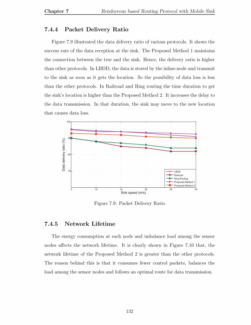
Chapter 7 Rendezvous based Routing Protocol with Mobile Sink
7.4.4 Packet Delivery Ratio
Figure 7.9 illustrated the data delivery ratio of various protocols. It shows the
success rate of the data reception at the sink. The Proposed Method 1 maintains
the connection between the tree and the sink. Hence, the delivery ratio is higher
than other protocols. In LBDD, the data is stored by the inline-node and transmit
to the sink as soon as it gets the location. So the possibility of data loss is less
than the other protocols. In Railroad and Ring routing the time duration to get
the sink’s location is higher than the Proposed Method 2. It increases the delay to
the data transmission. In that duration, the sink may move to the new location
that causes data loss.
5 10 15 20 25 30
70
80
90
100
Sink speed (m/s)
Da
ta d
eliv
ery
ra
tio
(%
)
LBDD
Railroad
Ring Routing
Proposed Method 1
Proposed Method 2
Figure 7.9: Packet Delivery Ratio
7.4.5 Network Lifetime
The energy consumption at each node and imbalance load among the sensor
nodes affects the network lifetime. It is clearly shown in Figure 7.10 that, the
network lifetime of the Proposed Method 2 is greater than the other protocols.
The reason behind this is that it consumes fewer control packets, balances the
load among the sensor nodes and follows an optimal route for data transmission.
132
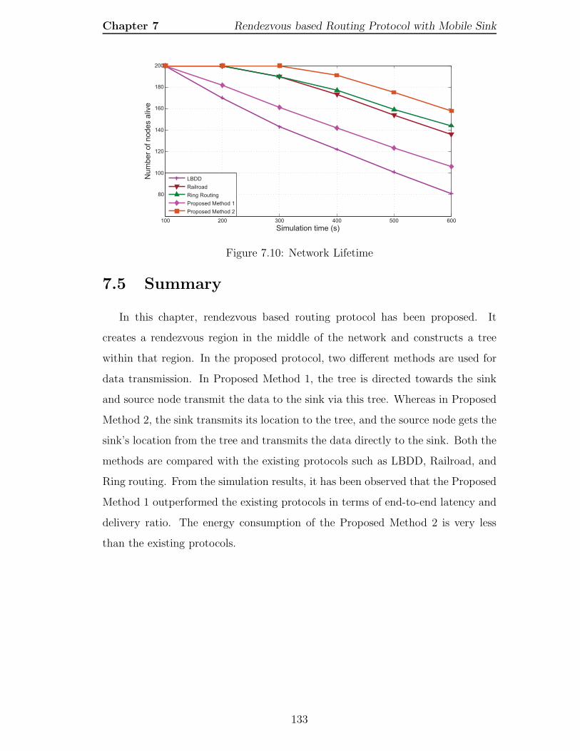
Chapter 7 Rendezvous based Routing Protocol with Mobile Sink
100 200 300 400 500 600
80
100
120
140
160
180
200
Simulation time (s)
Nu
mb
er
of
no
de
s a
live
LBDD
Railroad
Ring Routing
Proposed Method 1
Proposed Method 2
Figure 7.10: Network Lifetime
7.5 Summary
In this chapter, rendezvous based routing protocol has been proposed. It
creates a rendezvous region in the middle of the network and constructs a tree
within that region. In the proposed protocol, two different methods are used for
data transmission. In Proposed Method 1, the tree is directed towards the sink
and source node transmit the data to the sink via this tree. Whereas in Proposed
Method 2, the sink transmits its location to the tree, and the source node gets the
sink’s location from the tree and transmits the data directly to the sink. Both the
methods are compared with the existing protocols such as LBDD, Railroad, and
Ring routing. From the simulation results, it has been observed that the Proposed
Method 1 outperformed the existing protocols in terms of end-to-end latency and
delivery ratio. The energy consumption of the Proposed Method 2 is very less
than the existing protocols.
133

8
Conclusions
Future Research Directions

Chapter 8
Conclusions
The work presented in the thesis has been inspired by the energy constraint
of the sensor nodes. In this thesis, the protocols have been proposed for efficient
routing in WSN, and evaluations were made through the simulations using Castalia
(v3.2), a WSN simulator based on the OMNeT++ platform. In the thesis, six
routing protocols have been proposed, out of which, two protocols are based on
the static sink, and rests are based on the mobile sink.
The protocol MRP has been designed to improve the lifetime, latency and
reliability through discovering multiple paths between the source and the sink.
More than one routing paths are available for data transmission. If one path fails,
an alternate path is used to transmit the data. Sensor nodes could conserve the
energy by switching into the sleep mode if they were not involved in the routing
path. It has been observed that the control packet overhead for path discovery
and maintenance is very less. Thus, the improvement in the energy-efficiency has
been achieved.
The cluster based multipath routing protocol with static sink (CMRP) is
employed to reduce the transmission of redundant data and mitigate the traffic in
the network. Further, CMRP reduces the load on the sensor nodes and provides
more responsibility to the sink. Here, the sink handles cluster head selection,
routing path discovery and monitoring the energy level of the sensor nodes.
The sensor nodes only perform their basic functions like sensing, processing and
forwarding the data. CMRP resulted in the increase in lifetime, data delivery
ratio, and reduced end-to-end latency.
135

Conclusions
A tree based routing with mobile sink (TEDD) has been designed that
efficiently manage the mobile sink in the network. The sink is moving within
the network and gathering the data. A sensor node initiates the tree construction
and becomes the root node of the tree. The link is bidirectional between relay
nodes and unidirectional between a relay and non-relay node. Any sensor node
can transmit their data through the relay nodes. The links are managed according
to the sink position. TEDD is very robust and energy-efficient in the mobile sink
environment.
The proposed dense tree based routing protocol with mobile sink (DTRP) is
an extension of TEDD, which has two objectives such as minimization of control
overhead, and reduction of path length. Both the objectives were achieved by
reducing the number of relay nodes in the tree structure. The DTRP resulted in
the increase in the lifetime and reduced end-to-end latency.
The proposed clustered tree based routing protocol with mobile sink (CTRP)
has been designed to reduce the data traffic in the network and efficiently manage
the mobile sink. The traffic has been reduced by the cluster head, which used
aggregation technique. The number of cluster heads is restricted to the number
of grids presented in the network. The tree is constructed in the network using
the cluster heads as vertices. The data has been transmitted to the sink through
the tree structure. The CTRP has effectively managed the load among the sensor
nodes. It has been validated and compared with the TEDD and DTRP in terms
of energy-efficiency, network lifetime, end-to-end latency and data delivery ratio.
The proposed rendezvous based routing protocol with mobile sink (RRP) has
been designed for the time-sensitive applications, which efficiently transmit the
data to the mobile sink. Each sensor node can communicate with the rendezvous
region. In RRP, two data transmission methods have been proposed. In the first
method, source node directly sends their sensory data to the rendezvous region.
In the second method, the source node retrieves the sink’s current position and
transmits the data to the sink through intermediate nodes. It is found that the
end-to-end latency and data delivery ratio have been improved in the first proposed
136

Chapter 8 Conclusions
method. Whereas, energy consumption and network lifetime have been improved
in the second proposed method.
8.1 Future Research Directions
The research proposals made out of this thesis have opened several challenging
research directions, which can be further investigated. The proposed schemes
mostly deal with energy efficiency in routing protocol can be further extended to
improving energy efficiency in MAC layer. The routing protocol that supports
multiple static or mobile sinks will be the promising research direction to bring
energy-efficiency. The requirement of security is also an emerging area of research
in WSN. A light-weight security mechanism that requires low power, and less
computing cost must be developed for secure routing. Additionally, the design
of efficient routing protocol specific to real-time applications, which can offer
to improve the Quality-of-Services (QoS) like latency, reliability, packet loss and
throughput can be considered.
137

Bibliography
[1] M. Gholipour, A. T. Haghighat, and M. R. Meybodi, “Opportunistic Routing Algorithm
for Relay Node Selection in Wireless Sensor Networks,” IEEE Transactions on Industrial
Informatics, Vol. 11, No. 1, Pages 112 – 121, February 2015.
[2] A. Tiab and L. B. Medjkoune, “Routing in Industrial Wireless Sensor Networks: A
Survey,” Chinese Journal of Engineering, Vol. 2014, Pages 1 – 7, 2014.
[3] E. C. Whitman, “SOSUS: The Secret Weapon of Undersea Surveillance,” Undersea
Warfare magazine, Vol. 7, No. 2, Pages 1 – 5, 2005.
[4] C. Y. Chong and S. P. Kumar, “Sensor Networks: Evolution, Opportunities, and
Challenges,” Proceedings of the IEEE, Vol. 91, No. 8, Pages 1247 – 1256, August 2003.
[5] S. Patnaik, X. Li, and Y. M. Yang, Recent Development in Wireless
Sensor and Ad-hoc Networks. Springer, 2014, Vol. 1. [Online]. Available:
http://www.springer.com/us/book/9788132221289
[6] J. M. Kahn, R. H. Katz, and K. S. J. Pister, “Next Century Challenges: Mobile
Networking for Smart Dust,” In 5th annual ACM/IEEE International Conference on
Mobile Computing and Networking (MobiCom ’99), Pages 271 – 278, 1999.
[7] B. Krishnamachari, Networking Wireless Sensors. Cambridge University Press, 2005.
[Online]. Available: http://www.cambridge.org/9780521838474
[8] J. Wu, S. Dulman, P. Havinga, and T. Nieberg, “Experimental Study of Concurrent
Transmission in Wireless Sensor Networks,” In SAFE & ProRISC 2004, Pages 181 – 188,
November 2004.
[9] T. T. Vu, V. D. Nguyen, and H. M. Nguyen, “An Energy-Aware Routing Protocol for
Wireless Sensor Networks Based on K-Means Clustering,” In Recent Advances in Electrical
Engineering and Related Sciences, Vol. 282, Pages 297 – 306, 2014.
[10] P. Kuila and P. K. Jana, “Energy Efficient Clustering and Routing Algorithms for Wireless
Sensor Networks: Particle Swarm Optimization Approach,” Engineering Applications of
Artificial Intelligence, Vol. 33, Pages 127 – 140, August 2014.
138

Bibliography
[11] M. K. Mishra and M. M. Gore, “An Improved Forwarder Selection Approach for
Energy Aware Geographic Routing in Three Dimensional Wireless Sensor Networks,” In
International Conference on Communication, Computing & Security, Pages 166 – 171,
2011.
[12] W. Farjow, A. Chehri, H. T. Mouftah, and X. Fernando, “An Energy-Efficient Routing
Protocol for Wireless Sensor Networks through Nonlinear Optimization,” In International
Conference on Wireless Communications in Unusual and Confined Areas (ICWCUCA
’12), Pages 1 – 4, August 2012.
[13] M. Chawla, J. Singhai, and J. L. Rana, “Clustering in Mobile Ad-hoc Networks: A
Review,” International Journal of Computer Science and Information Security, Vol. 8,
No. 2, Pages 293 – 301, 2010.
[14] M. Rossi, M. Zorzi, and R. R. Rao, “Statistically Assisted Routing Algorithms (SARA) for
Hop Count based forwarding in Wireless Sensor Networks,” Wireless Networks, Vol. 14,
No. 1, Pages 55 – 70, January 2008.
[15] W. Liu, S. Zhang, and J. Fan, “A Diagnosis-Based Clustering and Multipath Routing
Protocol for Wireless Sensor Networks,” International Journal of Distributed Sensor
Networks, Vol. 2012, Pages 21 – 31, 2012.
[16] S. P. Singh and S. Sharma, “A Survey on Cluster Based Routing Protocols in Wireless
Sensor Networks,” In International Conference on Advanced Computing Technologies and
Applications (ICACTA ’15), Vol. 45, Pages 687 – 695, 2015.
[17] H. Lin and H. Uster, “Exact and Heuristic Algorithms for Data-Gathering Cluster-Based
Wireless Sensor Network Design Problem,” IEEE/ACM Transactions on Networking,
Vol. 22, No. 3, Pages 903 – 916, June 2014.
[18] D. Zhang, G. Li, K. Zheng, X. Ming, and Z. H. Pan, “An Energy-Balanced Routing Method
Based on Forward-Aware Factor for Wireless Sensor Networks,” IEEE Transactions on
Industrial Informatics, Vol. 10, No. 1, Pages 766 – 773, February 2014.
[19] J. I. Bangash, A. H. Abdullah, M. H. Anisi, and A. W. Khan, “A Survey of Routing
Protocols in Wireless Body Sensor Networks,” Sensors, Vol. 14, No. 1, Pages 1322 – 1357,
January 2014.
[20] T. Rault, A. Bouabdallah, and Y. Challal, “Energy Efficiency in Wireless Sensor Networks:
A Top-Down Survey,” Computer Networks, Vol. 67, No. 1, Pages 104 – 122, July 2014.
[21] L. Xie, Y. Shi, Y. T. Hou, W. Lou, H. D. Sheral, and S. F. Midkiff, “Multi-Node Wireless
Energy Charging in Sensor Networks,” IEEE/ACM Transactions on Networking, Vol. 23,
No. 2, Pages 437 – 450, April 2015.
139

Bibliography
[22] T. K. Jain, D. S. Saini, and S. V. Bhooshan, “Lifetime Optimization of a Multiple Sink
Wireless Sensor Network through Energy Balancing,” Journal of Sensors, Vol. 2015, Pages
1 – 6, 2015.
[23] M. Gholipour, A. T. Haghighat, and M. R. Meybodi, “Hop-by-Hop Traffic-Aware Routing
to Congestion Control in Wireless Sensor Networks,” EURASIP Journal on Wireless
Communications and Networking, Vol. 2015, No. 15, Pages 1 – 13, January 2015.
[24] M. Azharuddin and P. K. Jana, “A Distributed Algorithm for Energy Efficient and Fault
Tolerant Routing in Wireless Sensor Networks,” Wireless Networks, Vol. 21, No. 1, Pages
251 – 267, January 2015.
[25] B. Cheng, R. Du, B. Yang, W. Yu, C. Chen, and X. Guan, “An Accurate GPS-based
Localization in Wireless Sensor Networks: A GM-WLS Method,” In Parallel Processing
Workshops (ICPPW ’11), Pages 33 – 41, September 2011.
[26] Y. M. Lu and V. W. S. Wong, “GPS-free Positioning in Mobile Ad Hoc Networks,” Cluster
Computing, Vol. 5, No. 2, Pages 157 – 167, 2002.
[27] H. Akcan, V. K. andHerve Bronnimann, and A. Delis, “GPS-Free Node Localization
in Mobile Wireless Sensor Networks,” In 5th ACM International Workshop on Data
Engineering for Wireless and Mobile Access, Ser. MobiDE ’06, Pages 35 – 42, 2006.
[28] W. Heinzelman, A. Chandrakasan, and H. Balakrishnan, “Energy-Efficient
Communication Protocol for Wireless Microsensor Networks,” In 33rd Hawaii
International Conference on System Sciences (HICSS ’00), Pages 10 – 19, January
2000.
[29] O. Younis and S. Fahmy, “HEED: A Hybrid Energy-Efficient Distributed Clustering
Approach for Ad Hoc Sensor Networks,” IEEE Transactions on Mobile Computing, Vol. 3,
No. 4, Pages 366 – 379, December 2004.
[30] S. Lindsey and C. Raghavendra, “PEGASIS: Power-Efficient Gathering in Sensor
Information Systems,” In IEEE Aerospace Conference, Pages 1125 – 1130, 2002.
[31] H. Li, J. Cao, and J. Xiong, “Constructing Optimal Clustering Architecture for
Maximizing Lifetime in Large Scale Wireless Sensor Networks,” In 15th International
Conference on Parallel and Distributed Systems, Pages 182 – 189, 2009.
[32] O. Zytoune, Y. Fakhri, and D. Aboutajdine, “A Novel Energy Aware Clustering Technique
for Routing in Wireless Sensor Networks,” Wireless Sensor Network, Vol. 2010, No. 2,
Pages 233 – 238, March 2010.
[33] W. Naruephiphat and C. Charnsripinyo, “The Clustering Algorithm for Enhancing
Network Lifetime in Wireless Sensor Networks,” In Symposia and Workshops on
Ubiquitous, Autonomic and Trusted Computing (UIC-ATC ’09), Pages 240 – 245, July
2009.
140
Bibliography
[34] J. Y. Chang and P. H. Ju, “An Efficient Cluster-based Power Saving scheme for Wireless
Sensor Networks,” EURASIP Journal on Wireless Communications and Networking, Vol.
2012, No. 1, Pages 1 – 10, May 2012.
[35] S. D. Muruganthan, D. C. F. Ma, B. Rollyi, and A. Fapojuwo, “A centralized
energy-efficient routing protocol for wireless sensor networks,” IEEE Radio
Communications, Vol. 43, No. 3, Pages 8 – 13, 2005.
[36] C. Intanagonwiwat, R. Govindan, D. Estrin, J. Heidemann, and F. Silva, “Directed
Diffusion For Wireless Sensor Networking,” IEEE/ACM Transaction on Network, Vol. 11,
No. 1, Pages 2 – 16, February 2003.
[37] D. Ganesan, R. Govindan, S. Shenker, and D. Estrin, “Highly-resilient Energy-Efficient
Multipath Routing in Wireless Sensor Networks,” In 2nd ACM international symposium
on Mobile ad hoc networking & computing, Ser. MobiHoc ’01, Pages 251 – 254, 2001.
[38] Y. M. Lu and V. W. S. Wong, “An Energy-Efficient Multipath Routing Protocol for
Wireless Sensor Networks,” International Journal of Communication Systems, Vol. 20,
No. 7, Pages 747 – 766, July 2007.
[39] M. Maimour, “Maximally Radio-Disjoint Multipath Routing for Wireless Multimedia
Sensor Networks,” In 4th ACM workshop on Wireless Multimedia Networking and
Performance Modelling, Pages 26 – 31, 2008.
[40] Z. Wang, E. Bulut, and B. K. Szymanski, “Energy Efficient Collision Aware
Multipath Routing for Wireless Sensor Networks,” In IEEE international conference on
Communications, Pages 91 – 95, 2009.
[41] M. Radi, B. Dezfouli, K. A. Bakarand, S. A. Razak, and M. A. Nematbakhsh,
“Interference-Aware Multipath Routing Protocol for QoS Improvement in Event-Driven
Wireless Sensor Networks,” Tsinghua Science and Technology, Vol. 16, No. 5, Pages 475
– 490, 2011.
[42] D. S. J. D. Couto, D. Aguayo, J. Bicket, and R. Morris, “A High-Throughput Path
Metric for Multi-Hop Wireless Routing,” In 9th annual international conference on Mobile
computing and networking (MobiCom ’03), Pages 134 – 146, September 2003.
[43] M. Cherian and T. R. G. Nair, “Multipath Routing With Novel Packet Scheduling
Approach In Wireless Sensor Networks ,” International Journal of Computer Theory and
Engineering, Vol. 3, No. 5, Pages 666 – 670, 2011.
[44] B. Karp and H. T. Kung, “GPSR: Greedy Perimeter Stateless Routing for Wireless
Networks,” In 6th Annual International Conference on Mobile Computing and Networking,
Pages 243 – 254, 2000.
141

Bibliography
[45] Y. Xu, J. Heidemann, and D. Estrin, “Geography Informed Energy Conservation for
Ad-hoc Routing ,” In 7th Annual ACM/IEEE International Conference on Mobile
Computing and Networking, Pages 70 – 84, 2001.
[46] H. Zhang and H. Shen, “EEGR: Energy-Efficient Geographic Routing inWireless Sensor
Networks,” In International Conference on Parallel Processing (ICPP ’07), Pages 1 – 8,
2007.
[47] R. Alasem, A. Reda, and M. Mansou, “Location based Energy-Efficient Reliable Routing
Protocol for Wireless Sensor Networks,” In 10th WSEAS International Conference on
Electronics, Hardware, Wireless and Optical Communication, Pages 180 – 185, 2011.
[48] R. Ding and L. Yang, “A Reactive Geographic Routing Protocol for Wireless Sensor
Networks,” In 6th International Conference on Intelligent Sensors, Sensor Networks and
Information Processing (ISSNIP ’10), Pages 31 – 36, 2010.
[49] T. Y. Chen, H. W. Wei, C. R. Lee, F. N. Huang, T. sheng Hsu, and W. K. Shih,
“EEGRA: Energy Efficient Geographic Routing Algorithms for Wireless Sensor Network,”
In International Symposium on Pervasive Systems, Algorithms and Networks, Pages 104
– 113, 2012.
[50] T. Bagheri and A. Ghaffari, “RECM: Reliable and Energy effective Clustering based
Multipath Routing Algorithm for Wireless Sensor Networks,” In IEEE World Congress on
Information and Communication Technologies (WICT’11), Pages 1340 – 1345, December
2011.
[51] T. N. Quynh, T. T. Vinh, and M. B. T. Quynh, “Multipath Routing for Cluster-based
and Event-based Protocols in Wireless Sensor Networks,” In 3rd ACM Symposium on
Information and Communication Technology SoICT’12, Pages 172 – 179, 2012.
[52] M. R. Mazaheri, B. Homayounfar, and S. M. Mazinani, “QoS Based and Energy Aware
Multi-Path Hierarchical Routing Algorithm in WSNs,” Wireless Sensor Network, Vol. 4,
Pages 31 – 39, 2012.
[53] R. C. Jin, T. Gao, J. Y. Song, J. Y. Zou, and L. D. Wang, “Passive Cluster-based Multipath
Routing Protocol for Wireless Sensor Networks,” Wireless Networks, Vol. 19, No. 8, Pages
1851 – 1866, November 2013.
[54] S. Mueller, R. P. Tsang, and D. Ghosal, “An Efficient N-to-1 Multipath Routing Protocol
in Wireless Sensor Networks,” In IEEE International Conference on Mobile Adhoc and
Sensor Systems Conference, Pages 672 – 679, November 2005.
[55] I. T. Almalkawi, M. G. Zapata, and J. N. A. Karaki, “A Cross-Layer-Based
Clustered Multipath Routing with QoS-Aware Scheduling for Wireless Multimedia Sensor
Networks,” International Journal of Distributed Sensor Networks, Vol. 2012, Pages 1 – 11,
2012.
142

Bibliography
[56] M. S. Zaman and G. R. Murthy, “Clustered and Leveled Disjoint Multipath Routing
Algorithm for Wireless Sensor Networks,” In 1st IEEE Asian Himalayas International
Conference on Internet (AH-ICI ’09), Pages 1 – 5, November 2009.
[57] Y. H. Wang, C. H. Tsai, and H. J. Mao, “HMRP: Hierarchy-Based Multipath Routing
Protocol for Wireless Sensor Networks,” Tamkang Journal of Science and Engineering,
Vol. 9, No. 6, Pages 255 – 264, 2006.
[58] J. Yang, M. Xu, W. Zhao, and B. Xu, “A Multipath Routing Protocol Based on Clustering
and Ant Colony Optimization for Wireless Sensor Networks,” MDPI Sensors, Vol. 10,
Pages 4521 – 4540, May 2010.
[59] S. Okdem and D. Karaboga, “Routing in Wireless Sensor Networks Using an Ant Colony
Optimization (ACO) Router Chip ,” Sensors, Vol. 2009, No. 9, Pages 909 – 921, February
2009.
[60] L. Popa, A. Rostamizadeh, R. M. Karp, C. Papadimitriou, and I. Stoica, “Balancing
Traffic Load in Wireless Networks with Curveball Routing,” In 8th ACM International
Symposium on Mobile Ad Hoc Networking and Computing, Pages 170 – 179, September
2007.
[61] J. Li and P. Mohapatra, “Analytical modeling and mitigation techniques for The Energy
Hole Problem in Sensor Networks,” Pervasive Mobile Computing, Vol. 3, No. 3, Pages 233
– 254, June 2007.
[62] C. J. Lin, P. L. Chou, and C. F. Chou, “HCDD: Hierarchical Cluster based Data
Dissemination in Wireless Sensor Networks with Mobile Sink,” In International Conference
on Wireless Communications and Mobile Computing, Pages 1189 – 1194, July 2006.
[63] Y. H. Wang, K. F. Huang, P. F. Fu, and J. X. Wang, “Mobile Sink Routing Protocol
with Registering in Cluster-Based Wireless Sensor Networks,” In 5th International
Conferenceon on Ubiquitous Intelligence and Computing (UIC ’08), Pages 352 – 362, June
2008.
[64] J. Wang, Y. Yin, J. U. Kim, S. Lee, and C. F. Lai, “A Mobile-Sink Based Energy-Efficient
Clustering Algorithm for Wireless Sensor Networks,” In IEEE 12th International
Conference on Computer and Information Technology (CIT ’12), Pages 678 – 683, October
2012.
[65] N. C. Wang, P. C. Yeh, and Y. F. Huang, “An Energy-Aware Data Aggregation Scheme
for Grid-based Wireless Sensor Networks,” In International Conference on Wireless
Communications and Mobile Computing, Pages 487 – 492, October 2007.
[66] H. S. Kim, T. F. Abdelzaher, and W. H. Kwon, “Minimum-Energy Asynchronous
Dissemination to Mobile Sinks in Wireless Sensor Networks,” In 1st International
Conference on Embedded Networked Sensor Systems, Pages 193 – 204, October 2003.
143

Bibliography
[67] K. I. Hwang and D. seop Eom, “Adaptive Sink Mobility Management Scheme for
Wireless Sensor Networks,” In 3rd international conference on Ubiquitous Intelligence and
Computing, Pages 478 – 487, 2006.
[68] G. Wang, T. Wang, W. Jia, and M. Guo, “Local Update-Based Routing Protocol in
Wireless Sensor Networks with Mobile Sinks,” In IEEE International Conference on
Communications (ICC ’07), Pages 3094 – 3099, June 2007.
[69] K. I. Hwang, J. In, and D. seop Eom, “Distributed Dynamic Shared Tree for Minimum
Energy Data Aggregation of Multiple Mobile Sinks in Wireless Sensor Networks,” In 3rd
European conference on Wireless Sensor Networks, Pages 132 – 147, 2006.
[70] A. C. Viana, T. Herault, T. Largillier, S. Peyronnet, and F. Zaidi, “SUPPLE: A Flexible
Probabilistic Data Dissemination Protocol for Wireless Sensor Networks,” In 13th ACM
International Conference on Modeling, Analysis, and Simulation of Wireless and Mobile
Systems, Pages 385 – 392, 2010.
[71] Y. Faheem and S. Boudjit, “SN-MPR: A Multi-Point Relay Based Routing Protocol
for Wireless Sensor Networks,” In IEEE/ACM International Conference on Green
Computing and Communications & International Conference on Cyber, Physical and
Social Computing, Pages 761 – 767, 2010.
[72] A. Qayyum, L. Viennot, and A. Laouiti, “Multipoint Relaying for Flooding Broadcast
Messages in Mobile Wireless Networks,” In 35th Annual Hawaii International Conference
on System Sciences, Pages 3866 – 3875, January 2002.
[73] H. Luo, F. Ye, J. Cheng, S. Lu, and L. Zhang, “TTDD: Two-Tier Data Dissemination
in Large-Scale Wireless Sensor Networks,” Wireless Networks, Vol. 11, Pages 161 – 175,
2005.
[74] K. Kweon, H. Ghim, J. Hong, and H. Yooni, “Grid-Based Energy-Efficient Routing
from Multiple Sources to Multiple Mobile Sinks in Wireless Sensor Networks,” In 4th
International Symposium on Wireless Pervasive Computing (ISWPC ’09), Pages 1 – 5,
February 2009.
[75] E. B. Hamida and G. Cheliusi, “A Line-Based Data Dissemination protocol for
Wireless Sensor Networks with Mobile Sink,” In IEEE International Conference on
Communications (ICC ’08), Pages 2201 – 2205, 2008.
[76] J. H. Shin, J. Kim, K. Park, and D. Park, “Railroad: Virtua Infrastructure for
Data Dissemination in Wireless Sensor Networks,” In 2nd ACM International Workshop
on Performance Evaluation of Wireless Ad Hoc, Sensor, and Ubiquitous Networks
(PE-WASUN ’05), Pages 168 – 174, 2005.
[77] C. Tunca, S. Isik, M. Y. Donmez, and C. Ersoy, “Ring routing: An energy-Efficient Routing
Protocol for Wireless Sensor Networks with a Mobile Sink,” IEEE Transactions on Mobile
Computing, Vol. 13, No. 11, Pages 1 – 15, November 2014.
144

Bibliography
[78] K. Akkaya and M. Younis, “A Survey on Routing Protocols for Wireless Sensor Networks,”
Ad Hoc Networks, Vol. 3, No. 1, Pages 325 – 349, 2005.
[79] J. N. A. Karaki and A. E. Kamal, “Routing Techniques in Wireless Sensor Networks: A
Survey,” IEEE Wireless Communications, Vol. 11, No. 6, Pages 6 – 28, December 2004.
[80] D. Ye, M. Zhang, and Y. Yang, “A Multi-Agent Framework for Packet Routing in Wireless
Sensor Networks,” Sensors, Vol. 15, No. 5, Pages 10 026 – 10 047, April 2015.
[81] T. N. Le, P. H. J. Chong, X. J. Li, and W. Y. Leong, “A Simple Grid-Based Localization
Technique in Wireless Sensor Networks for Forest Fire Detection,” In 2nd International
Conference on Communication Software and Networks, Pages 93 – 98, February 2010.
[82] L. Kenc and J. Y. L. Boudec, “Adaptive Load Sharing for Network Processors,”
IEEE/ACM Transactions on Networking, Vol. 16, No. 2, Pages 293 – 309, April 2008.
[83] J. Wang, Y. Niu, J. Cho, and S. Lee, “Analysis of Energy Consumption in Direct
Transmission and Multi-hop Transmission for Wireless Sensor Networks,” In 3rd
International IEEE Conference on Signal-Image Technologies and Internet-Based System
(SITIS ’07), Pages 275 – 280, 2007.
[84] J. Xu, W. Liu, F. Lang, Y. Zhang, and C. Wang, “Distance Measurement Model Based
on RSSI in WSN,” Wireless Sensor Network, Vol. 2010, No. 2, Pages 606 – 611, August
2007.
[85] V. T. Quang and T. Miyoshi, “A Transmission Range Adjustment Algorithm to Avoid
Energy Holes in Wireless Sensor Networks,” In 8th Asia-Pacific Symposium on Information
and Telecommunication Technologies (APSITT ’10), Pages 1 – 6, June 2010.
[86] R. K. Batwada, M. Tripathi, M. S. Gaur, and V. Laxmi, “An Approach for Prolonging the
Life Time of Wireless Sensor Network,” In 2nd International Conference on Information
and Network Technology (ICINT ’12), Vol. 27, Pages 264 – 268, 2012.
[87] S. Paul, S. Nandi, and I. Singh, “A Dynamic Balanced-Energy Sleep Scheduling Scheme
in Heterogeneous Wireless Sensor Network,” In 16th IEEE International Conference on
Networks (ICON ’08), Pages 1 – 6, December 2008.
[88] S. Basagni and C. Petrioli, “Controlled Vs. Uncontrolled Mobility in Wireless Sensor
Networks: Some Performance Insights,” In IEEE 66th Vehicular Technology Conference
(VTC ’07), Pages 269 – 273, 2007.
[89] M. I. Khan, W. N. Gansterer, and G. Haring, “Static vs. Mobile sink,” Computer
Communication, Vol. 36, No. 9, Pages 965 – 978, August 2013.
[90] X. H. Li, S. H. Hong, and K. L. Fang, “Location-Based Self-Adaptive Routing Algorithm
for Wireless Sensor Networks in Home Automation,” EURASIP Journal on Embedded
Systems, Vol. 2011, Pages 1 – 15, January 2011.
145

Bibliography
[91] W. Lou, W. Liu, and Y. Zhang, “Performance Optimization Using Multipath Routing
in Mobile Ad Hoc and Wireless Sensor Networks,” In Combinatorial Optimization in
Communication Networks, Ser. Combinatorial Optimization, Vol. 18, Pages 117 – 146,
2006.
[92] P. Hurni and T. Braun, “Energy-Efficient Multi-path Routing in Wireless Sensor
Networks,” In 7th International Conference on Ad-hoc, Mobile and Wireless Networks,
Pages 72 – 85, 2008.
[93] M. Radi, B. Dezfouli, and S. A. R. K. A. Bakar, “LIEMRO: A Low-Interference
Energy-Efficient Multipath Routing Protocol for Improving QoS in Event-Based Wireless
Sensor Networks,” In 4th IEEE International Conference on Sensor Technologies and
Applications, Pages 551 – 557, 2010.
[94] M. Radi, B. Dezfouli, K. A. Bakar, and M. Lee, “Multipath Routing in Wireless Sensor
Networks: Survey and Research Challenges,” MDPI Sensors, Vol. 12, No. 1, Pages 650 –
685, January 2012.
[95] T. V. Dam and A. K. Langendoen, “An Adaptive Energy-Efficient Mac Protocol for
Wireless Sensor Networks,” In 1st international conference on Embedded networked sensor
systems (SenSys ’03), Pages 171 – 180, 2003.
[96] B. Wendi, A. Heinzelman, P. Chandrakasan, and H. Balakrishnan, “An
Application-Specific Protocol Architecture for Wireless Microsensor Networks,” IEEE
Tranactions on Wireless Communications, Vol. 1, No. 4, Pages 660 – 670, October 2002.
[97] Q. Wang, M. Hempstead, and W. Yang, “A Realistic Power Consumption Model
for Wireless Sensor Network Devices,” In IEEE International Conference on Sensing,
Communication, and Networking (SECON ’6), Pages 286 – 295, 2006.
[98] Castalia Wireless Sensor Network Simulator website and user manual. [Online]. Available:
http://castalia.npc.nicta.com.au/
[99] A. Varga. OMNeT++ Home Page. [Online]. Available:
http://www.hit.bme.hu/phd/vargaa/omnetpp.htm
[100] MICAz Wireless Measurement System Datasheet, Crossbow Technology, Inc. . [Online].
Available: http://www.openautomation.net/uploadsproductos/micaz datasheet.pdf
[101] V. Cionca, T. Newe, and V. Dadarlat, “TDMA Protocol Requirements for Wireless
Sensor Networks,” In 2nd IEEE International Conference on Sensor Technologies and
Applications, Pages 30 – 35, Aug 2008.
[102] M. Perillo, Z. Cheng, andW. Heinzelman, “On the problem of unbalanced load distribution
in wireless sensor networks,” In IEEE Global Telecommunications Conference Workshops
(GlobeCom ’04), Pages 74 – 79, December 2004.
146

Bibliography
[103] M. Perillo and Z. Cheng, “An analysis of Strategies for Mitigating the Sensor Network
Hot Spot Problem,” In 2nd Annual International Conference on Mobile and Ubiquitous
Systems: Networking and Services (MobiQuitous ’05), Pages 474 – 478, July 2005.
[104] E. B. Hamidaand and G. Chelius, “Strategies for Data Dissemination to Mobile Sinks
in Wireless Sensor Networks,” IEEE Tranactions on Wireless Communications, Vol. 15,
No. 6, Pages 31 – 37, December 2008.
[105] J. Broch, D. A. Maltz, D. B. Johnson, Y. C. Hu, and J. Jetcheva, “A Performance
Comparison of Multi-hop Wireless Ad Hoc Network Routing Protocols,” In 4th Annual
ACM/IEEE International Conference on Mobile Computing and Networking, Pages 85 –
97, 1998.
[106] R. Akl and U. Sawant, “Grid-based Coordinated Routing in Wireless Sensor Networks,”
In 4th IEEE Consumer Communications and Networking Conference (CCNC ’07), Pages
860 – 864, January 2007.
[107] Z. Zhou, X. Xiang, X. Wang, and J. Pan, “An Energy-Efficient Data Dissemination
Protocol in Wireless Sensor Networks,” In International Symposium on World of Wireless,
Mobile and Multimedia Networks (WOWMOM ’06), Pages 13 – 22, January 2006.
[108] Y. Zhuang, J. Pan, and G. Wu, “Energy-Optimal Grid-Based Clustering in Wireless
Microsensor Networks,” In 29th IEEE International Conference on Distributed Computing
Systems Workshops (ICDCS Workshops ’09), Pages 96 – 102, June 2009.
147

Dissemination of Work
Journals
1. Suraj Sharma, Pratik Agarwal and S. K. Jena, EAMRP: Energy Aware Multipath
Routing Protocol for Wireless Sensor Networks˝, Accepted for Publication In
International Journal of Information & Communication Technology, Special Issue on:
Advances in Wireless Sensor Networks and their Applications, Inderscience Publishers,
February, 2015.
2. Suraj Sharma and S. K. Jena, Cluster based Multipath Routing Protocol for Wireless
Sensor Networks˝, Computer Communication Review, ACM, Volume 45, Issue 2, Pages
14-20, 2015.
3. Suraj Sharma and S. K. Jena, Data Dissemination Protocol for Mobile Sink in
Wireless Sensor Networks˝, Journal of Computational Engineering, Hindawi Publishing
Corporation, Volume 2014, Pages 1-10, 2014.
4. Suraj Sharma and S. K. Jena, Energy Aware Tree based Routing Protocol for Wireless
Sensor Networks˝, Communicated In Digital Communications and Networks, Elsevier,
2015.
5. Suraj Sharma and S. K. Jena, A Virtual Infrastructure based Energy Efficient
Routing Protocol for Wireless Sensor Networks˝, Communicated In Wireless Personal
Communications, Springer, 2015.
Conferences
1. Suraj Sharma, Pratik Agarwal and S. K. Jena, Energy Aware Multipath Routing
Protocol for Wireless Sensor Networks˝, In Fourth International Conference on Networks
& Communications (NetCom), Lecture Notes in Electrical Engineering, Springer, Volume
131, Pages 753-760, 2013.
2. Suraj Sharma, Dupatta Suresh and S. K. Jena, VGBST: A Virtual Grid-Based
Backbone Structure Type Scheme for Mobile Sink based Wireless Sensor Networks˝,
In International Conference on Advanced Research in Computer Science Engineering &
Technology (ICARCSET), ACM, Pages 1-5, 2015.
148

Publications
3. Suraj Sharma and S. K. Jena, A Cluster-Tree based Data Dissemination Routing
Protocol˝, In Eleventh International Multi Conference on Information Processing (IMCIP
’15), Elsevier, Pages 7-13, August 2015.
4. Suraj Sharma and S. K. Jena, A Virtual Infrastructure based Routing Protocol for
Wireless Sensor Networks˝, In 12th IEEE India International Conference (INDICON ’15),
IEEE, 17-20 December 2015.
Book Chapter
1. Suraj Sharma and S. K. Jena Routing protocol in Wireless Sensor Networks: Research
Directions˝, Communicated In Handbook of Research on Advanced Wireless Sensor
Network Applications, Protocols, and Architectures, IGI Global publisher, USA, 2015.
149

Resume
Suraj Sharma
Assistant Professor
IIIT Bhubaneswar
Gothapatna, Malipada,
Bhubaneswar - 751003, Odisha, India
Ph: +91-674-6636682 (O), +91-9861298939 (M)
e-mail: [email protected]
Qualification
• Doctor of Philosophy (Continuing)
National Institute of Technology Rourkela, India
• Master of Technology
Computer Science and Engineering
National Institute of Technology Rourkela, India [8.85 CGPA]
• Bachelor of Engineering
Computer Science and Engineering
Pt. Ravi Shankar Shukla University Raipur, India [75%]
• Higher Secondary
Government Higher Secondary School Marwahi, Chhattisgarh, India [75%]
• Matriculation
Government Higher Secondary School Marwahi, Chhattisgarh, India [76%]
Publications
• 06 Journal Articles
• 07 Conference Papers
• 01 Book Chapters
Permanent Address
150

Resume
Plot# C-30, Amolavilla Colony, Seepat Road
Bilaspur – 495001, Chhattisgarh, India.
Date of Birth
November 03, 1984
151