Tribhuvan UniversityInstitute of Science and Technology

Off-line Nepali Handwritten CharacterRecognition Using MLP and RBF Neural

Networks

DissertationSubmitted to

Central Department of Computer Science & Information TechnologyKirtipur, Kathmandu, Nepal

In partial fulfillment of the requirementsfor the Master’s Degree in Computer Science & Information Technology

ByAshok Kumar PantDate: 05 June, 2012

Tribhuvan UniversityInstitute of Science and Technology

Off-line Nepali Handwritten CharacterRecognition Using MLP and RBF Neural

Networks

DissertationSubmitted to

Central Department of Computer Science & Information TechnologyKirtipur, Kathmandu, Nepal

In partial fulfillment of the requirementsfor the Master’s Degree in Computer Science & Information Technology

ByAshok Kumar PantDate: 05 June, 2012

SupervisorProf. Dr. Shashidhar Ram Joshi

Co-SupervisorDr. Sanjeeb Prasad Panday

Tribhuvan UniversityInstitute of Science and Technology

Central Department of Computer Science & Information Technology

Student’s Declaration

I hereby declare that I am the only author of this work and that no sources other than the listedhere have been used in this work.

... ... ... ... ... ... ... ...Ashok Kumar PantDate: 05 June, 2012

Supervisor’s Recommendation

I hereby recommend that this dissertation prepared under my supervision by Mr. Ashok Ku-mar Pant entitled “Off-line Nepali Handwritten Character Recognition Using MLP andRBF Neural Networks” in partial fulfilment of the requirements for the degree of M.Sc. inComputer Science and Information Technology be processed for the evaluation.

... ... ... ... ... ... ... ... ...Prof. Dr. Shashidhar Ram JoshiDepartment of Electronics & Computer Engineering,Institute of Engineering,Pulchowk, Nepal

Date: 05 June, 2012

Tribhuvan UniversityInstitute of Science and Technology

Central Department of Computer Science & Information Technology

LETTER OF APPROVAL

We certify that we have read this dissertation and in our opinion it is satisfactory in the scopeand quality as a dissertation in the partial fulfillment for the requirement of Masters Degree inComputer Science and Information Technology.

Evaluation Committee

... ... ...... ... ... ... ... ... ... ... ...... ... ... ... ... ... ... ... ... ...Asst. Prof. Nawaraj Paudel Prof. Dr. Shashidhar Ram Joshi

Central Department of Computer Science Department of Electronics & Computer& Information Technology, Engineering, Institute of Engineering,

Tribhuvan University, Kathmandu, Nepal Pulchowk, Kathmandu, Nepal(Act. Head) (Supervisor)

... ... ...... ... ... ... ... ... ... ... ...... ... ... ... ... ...Assoc. Prof. Mr. Bal Krishna Bal Mr. Bishnu Gautam

(External Examinar) (Internal Examinar)

Date: 22 June, 2012

ACKNOWLEDGEMENTS

First and above all, I thank God for his love and guidance of all the time. I submit my gratitudeto the Almighty who gave ability, strength and confidence in me to complete this work. Withouthis mercy this would never come to be today’s reality. My life is so blessed because of him.

With deep sense of gratefulness I express my genuine thanks to my respected and worthysupervisor Prof. Dr. Shashidhar Ram Joshi, Head of Electronics & Computer EngineeringDepartment( Kathmandu, Nepal) for his valuable guidance in carrying out this work under hiseffective supervision and enlightenment.

I want to express my deep thanks to my honoured co-supervisor Dr. Sanjeeb Prasad Pandayof Electronics & Computer Engineering Department( Kathmandu, Nepal) for his inspiration,trust, the insightful discussion, thoughtful guidance, critical comments, and correction of thethesis.

I would like to thank my respected promoter Assoc. Prof. Dr. Tank Nath Dhamala, Headof Computer Science & IT Department,TU( Kathmandu, Nepal) for his encouragement andguidance.

My special thanks to Ms. Bhima Basnet of P.K. Campus( Kathmandu, Nepal) for her help inNepali handwritten character database creation and Ms. Rama Basnet of Sociology Depart-ment, TU(Kathmandu, Nepal) for her encouragement and help while writing the thesis. I amthankful to colleague Harendra Raj Bist for his through full reading and corrections of thedocument. Also, I am thankful to dear Ganga Ram Rimal for his technical help and support.

I want to thank Mr. Dinesh Dileep Gaurav, Ph.D student of Indian Institute of Science,Bangalore, India for his source code for directional feature extraction from character imageswhich I got from Mathwork Website. I also want to convey my thanks to MATLAB developerteam.

I am also thankful to all the staff members of the Department of Computer Science, TU (Kath-mandu, Nepal) for their full cooperation and help.

Thanks to all my close friends for their supports and help in creation of off-line Nepali hand-written database.

Finally, I thank my family for their love, support and encouragement.

i

ABSTRACT

An off-line Nepali handwriting recognition, based on the neural networks, is described in thisresearch work. For the recognition of off-line handwritings with high classification rate a goodset of features as a descriptor of image is required. Two important categories of the features aredescribed, geometric and statistical features for extracting information from character images.Directional features are extracted from geometry of skeletonized character image and statisticalfeatures are extracted from the pixel distribution of skeletonized character image. The researchprimarily concerned with the problem of isolated handwritten character recognition for Nepalilanguage. Multilayer Perceptron (MLP) & Radial Basis Function (RBF) classifiers are used forclassification. The principal contributions presented here are preprocessing, feature extractionand MLP & RBF classifiers. The another important contribution is the creation of benchmarkdataset for off-line Nepali handwritings. There are three datasets for Nepali handwritten nu-merals, Nepali handwritten vowels and Nepali handwritten consonants respectively. Nepalihandwritten numeral dataset contains total 288 samples for each 10 classes of Nepali numerals,Nepali handwritten vowel dataset contains 221 samples for each 12 classes of Nepali vowelsand Nepali handwritten consonant dataset contains 205 samples for each 36 classes of Nepaliconsonants. The strength of this research is efficient feature extraction and the comprehensiveclassification schemes due to which, the recognition accuracy of 94.44% is obtained for Nepalihandwritten numeral dataset, 86.04% is obtained for Nepali handwritten vowel dataset and80.25% is obtained for Nepali handwritten consonant dataset.

Keywords:

Off-line handwriting recognition, Image processing, Neural networks, Multilayer perceptron,Radial basis function, Preprocessing, Feature extraction, Nepali handwritten datasets

ii

To my dear father ...

iii

TABLE OF CONTENTS

Acknowledgement i

Abstract ii

List of Figures vii

List of Tables viii

Abbreviations ix

1 INTRODUCTION 11.1 Introduction . . . . . . . . . . . . . . . . . . . . . . . . . . . . . . . . . . . . 1

1.1.1 Motivation . . . . . . . . . . . . . . . . . . . . . . . . . . . . . . . . . 11.1.2 On-line versus Off-line Recognition . . . . . . . . . . . . . . . . . . . 21.1.3 Nepali Natural Handwriting . . . . . . . . . . . . . . . . . . . . . . . 21.1.4 Application of Off-line Nepali Handwriting Recognition System . . . . 31.1.5 Human performance in recognizing Handwritten Texts . . . . . . . . . 31.1.6 Artificial Neural Networks . . . . . . . . . . . . . . . . . . . . . . . . 3

1.1.6.1 History of Artificial Neural Networks . . . . . . . . . . . . . 41.1.6.2 Real Life Applications of Artificial Neural Networks . . . . . 5

1.2 Challenges . . . . . . . . . . . . . . . . . . . . . . . . . . . . . . . . . . . . . 51.3 Problem Definition . . . . . . . . . . . . . . . . . . . . . . . . . . . . . . . . 61.4 Objectives . . . . . . . . . . . . . . . . . . . . . . . . . . . . . . . . . . . . . 61.5 Contribution of this Thesis . . . . . . . . . . . . . . . . . . . . . . . . . . . . 71.6 Outline of the Thesis . . . . . . . . . . . . . . . . . . . . . . . . . . . . . . . 7

2 Literature Review 82.1 Previous Work . . . . . . . . . . . . . . . . . . . . . . . . . . . . . . . . . . . 82.2 Individual Character Recognition . . . . . . . . . . . . . . . . . . . . . . . . . 92.3 Word Recognition . . . . . . . . . . . . . . . . . . . . . . . . . . . . . . . . . 92.4 Preprocessing . . . . . . . . . . . . . . . . . . . . . . . . . . . . . . . . . . . 92.5 Feature Extraction . . . . . . . . . . . . . . . . . . . . . . . . . . . . . . . . . 102.6 Recognition Methods . . . . . . . . . . . . . . . . . . . . . . . . . . . . . . . 10

2.6.1 Template Matching . . . . . . . . . . . . . . . . . . . . . . . . . . . . 102.6.2 Statistical Techniques . . . . . . . . . . . . . . . . . . . . . . . . . . . 102.6.3 Structural Techniques . . . . . . . . . . . . . . . . . . . . . . . . . . . 112.6.4 Neural Network Techniques . . . . . . . . . . . . . . . . . . . . . . . 11

3 SYSTEM OVERVIEW 123.1 Image Acquisition . . . . . . . . . . . . . . . . . . . . . . . . . . . . . . . . . 12

iv

3.2 Image Preprocessing . . . . . . . . . . . . . . . . . . . . . . . . . . . . . . . 143.3 Feature Extraction . . . . . . . . . . . . . . . . . . . . . . . . . . . . . . . . . 143.4 Recognition . . . . . . . . . . . . . . . . . . . . . . . . . . . . . . . . . . . . 15

4 RESEARCH METHODOLOGY 164.1 Image Preprocessing . . . . . . . . . . . . . . . . . . . . . . . . . . . . . . . 16

4.1.1 RGB to Grayscale Conversion . . . . . . . . . . . . . . . . . . . . . . 174.1.2 Noise Removal . . . . . . . . . . . . . . . . . . . . . . . . . . . . . . 174.1.3 Image Segmentation . . . . . . . . . . . . . . . . . . . . . . . . . . . 184.1.4 Image Inversion . . . . . . . . . . . . . . . . . . . . . . . . . . . . . . 184.1.5 Universe of Discourse . . . . . . . . . . . . . . . . . . . . . . . . . . 194.1.6 Size Normalization . . . . . . . . . . . . . . . . . . . . . . . . . . . . 194.1.7 Image Skeletonization . . . . . . . . . . . . . . . . . . . . . . . . . . 19

4.2 Feature Extraction . . . . . . . . . . . . . . . . . . . . . . . . . . . . . . . . . 214.2.1 Directional Features . . . . . . . . . . . . . . . . . . . . . . . . . . . . 214.2.2 Moment Invariant Features . . . . . . . . . . . . . . . . . . . . . . . . 224.2.3 Euler Number . . . . . . . . . . . . . . . . . . . . . . . . . . . . . . . 234.2.4 Normalized Area of Character Skeleton . . . . . . . . . . . . . . . . . 244.2.5 Centroid of Image . . . . . . . . . . . . . . . . . . . . . . . . . . . . . 244.2.6 Eccentricity . . . . . . . . . . . . . . . . . . . . . . . . . . . . . . . . 24

4.3 Training and Testing . . . . . . . . . . . . . . . . . . . . . . . . . . . . . . . 254.3.1 Multilayer Feedforward Backpropagation Network . . . . . . . . . . . 25

4.3.1.1 Levenberg-Marquardt Learning Algorithm . . . . . . . . . . 264.3.1.2 Gradient descent with momentum and adaptive learning rate . 28

4.3.2 Radial Basis Function Network . . . . . . . . . . . . . . . . . . . . . . 294.3.2.1 Orthogonal Least Square Training Algorithm . . . . . . . . . 30

4.3.3 Performance Metrics . . . . . . . . . . . . . . . . . . . . . . . . . . . 31

5 IMPLEMENTATION 325.1 MATLAB . . . . . . . . . . . . . . . . . . . . . . . . . . . . . . . . . . . . . 325.2 Image Processing Toolbox . . . . . . . . . . . . . . . . . . . . . . . . . . . . 335.3 Neural Network Toolbox . . . . . . . . . . . . . . . . . . . . . . . . . . . . . 335.4 Feature Vector Creation . . . . . . . . . . . . . . . . . . . . . . . . . . . . . . 34

6 NEPALI HANDWRITTEN DATASETS 376.1 Dataset Creation Procedure . . . . . . . . . . . . . . . . . . . . . . . . . . . . 376.2 Nepali Handwritten Consonant Dataset . . . . . . . . . . . . . . . . . . . . . . 386.3 Nepali Handwritten Vowel Dataset . . . . . . . . . . . . . . . . . . . . . . . . 386.4 Nepali Handwritten Numeral Dataset . . . . . . . . . . . . . . . . . . . . . . . 39

7 EXPERIMENTATIONS AND RESULTS 40

8 CONCLUSION 498.1 Conclusion . . . . . . . . . . . . . . . . . . . . . . . . . . . . . . . . . . . . 498.2 Future Scope . . . . . . . . . . . . . . . . . . . . . . . . . . . . . . . . . . . 50

Appendix A Neural Network Parameters 51A.1 Nguyen–Widrow Weights Initialization . . . . . . . . . . . . . . . . . . . . . . 51A.2 Activation Function . . . . . . . . . . . . . . . . . . . . . . . . . . . . . . . . 51

v

Appendix B Sample Source Codes 53

vi

LIST OF FIGURES

1.1 Sample of Nepali Handwritten Consonants. . . . . . . . . . . . . . . . . . . . 21.2 Sample of Nepali Handwritten Vowels. . . . . . . . . . . . . . . . . . . . . . . 31.3 Sample of Nepali Handwritten Numerals. . . . . . . . . . . . . . . . . . . . . 31.4 A Physical Neuron. . . . . . . . . . . . . . . . . . . . . . . . . . . . . . . . . 41.5 An Artificial Neuron. . . . . . . . . . . . . . . . . . . . . . . . . . . . . . . . 4

3.1 Off-line Handwriting Recognition System. . . . . . . . . . . . . . . . . . . . . 123.2 Image Slicing. . . . . . . . . . . . . . . . . . . . . . . . . . . . . . . . . . . . 133.3 Image Acquisition. . . . . . . . . . . . . . . . . . . . . . . . . . . . . . . . . 133.4 Image Preprocessing. . . . . . . . . . . . . . . . . . . . . . . . . . . . . . . . 143.5 Feature Extraction. . . . . . . . . . . . . . . . . . . . . . . . . . . . . . . . . 143.6 Training and Testing. . . . . . . . . . . . . . . . . . . . . . . . . . . . . . . . 15

4.1 RGB to Grayscale Conversion. . . . . . . . . . . . . . . . . . . . . . . . . . . 174.2 Noise Removal. . . . . . . . . . . . . . . . . . . . . . . . . . . . . . . . . . . 174.3 Image Binarization. . . . . . . . . . . . . . . . . . . . . . . . . . . . . . . . . 184.4 Image Negatives. . . . . . . . . . . . . . . . . . . . . . . . . . . . . . . . . . 194.5 Universe of Discourse. . . . . . . . . . . . . . . . . . . . . . . . . . . . . . . 194.6 Size Normalization. . . . . . . . . . . . . . . . . . . . . . . . . . . . . . . . . 204.7 Binary Image Skeletonization. . . . . . . . . . . . . . . . . . . . . . . . . . . 214.8 Feedforward Multilayer Perceptron. . . . . . . . . . . . . . . . . . . . . . . . 264.9 RBF Neural Network. . . . . . . . . . . . . . . . . . . . . . . . . . . . . . . . 29

5.1 Nepali consonant letter ’ka’. . . . . . . . . . . . . . . . . . . . . . . . . . . . 345.2 Letter ’ka’ as binary matrix. . . . . . . . . . . . . . . . . . . . . . . . . . . . . 345.3 Zoned images . . . . . . . . . . . . . . . . . . . . . . . . . . . . . . . . . . . 34

6.1 Nepali Handwritten Consonants. . . . . . . . . . . . . . . . . . . . . . . . . . 386.2 Nepali Handwritten Vowels. . . . . . . . . . . . . . . . . . . . . . . . . . . . 386.3 Nepali Handwritten Numerals. . . . . . . . . . . . . . . . . . . . . . . . . . . 39

7.1 Recognition Accuracy of Off-line Handwriting Recognition Systems. . . . . . . 417.2 Training Time of Off-line Handwriting Recognition Systems. . . . . . . . . . . 427.3 Recognition Accuracy of Each Numeral Classes. . . . . . . . . . . . . . . . . 437.4 Recognition Accuracy of Each Vowel Classes. . . . . . . . . . . . . . . . . . . 447.5 Recognition Accuracy of Each Consonant Classes. . . . . . . . . . . . . . . . 48

A.1 Hyperbolic tangent sigmoid activation function. . . . . . . . . . . . . . . . . . 52

vii

LIST OF TABLES

7.1 Neural Network Configurations. . . . . . . . . . . . . . . . . . . . . . . . . . 407.2 Recognition Results. . . . . . . . . . . . . . . . . . . . . . . . . . . . . . . . 417.3 Recognition Results For Individual Numerals. . . . . . . . . . . . . . . . . . . 427.4 Confusion Matrix of Numeral Dataset Testing. . . . . . . . . . . . . . . . . . . 437.5 Recognition Results For Individual Vowels. . . . . . . . . . . . . . . . . . . . 447.6 Confusion Matrix of Vowel Dataset Testing. . . . . . . . . . . . . . . . . . . . 447.7 Recognition Results For Individual Characters. . . . . . . . . . . . . . . . . . 457.8 Confusion Matrix (I) of Consonant Dataset Testing. . . . . . . . . . . . . . . . 467.9 Confusion Matrix (II) of Consonant Dataset Testing. . . . . . . . . . . . . . . . 47

viii

LIST OF ABBREVIATIONS

ADALINE (ADAptive LInear Element)

ANN Artificial Neural Network

CM Confusion Matrix

CR Character Recognition

GDMA Gradient Descent with Momentum & Adaptive Learning Rate

HWR Handwriting Recognition

IPT Image Processing Toolbox

LM Levenberg-Marquardt

LMS Least Mean Square

LS Least Square

MAT Medial Axis Transformation

MLP Multilayer Perceptron

NNT Neural Network Toolbox

OCR Optical Character Recognition

OLS Orthogonal Least Square

RBF Radial Basis Function

RBFNN Radial Basis Function Neural Network

SVM Support Vector Machine

VLSI Very Large Scale Integration

ix

Chapter 1

INTRODUCTION

1.1 Introduction

Handwriting Recognition is the mechanism for transforming the written text into a symbolicrepresentation. Off-line handwriting recognition is the task of determining what characters orwords are present in a digital image of handwritten text. The problem of handwriting recog-nition can be viewed as a classification problem where we need to identify the most suitablecharacter the given figure matches to. It is a sub-field of Optical Character Recognition (OCR),whose domain can be machine-print or handwriting but is more commonly machine-print.Handwriting Recognition plays an essential role in many human computer interaction appli-cations including cheque verification, mail sorting, office automation, handwritten form verifi-cation, etc.

1.1.1 Motivation

Handwriting recognition is a special problem in the domain of pattern recognition and machineintelligence. The field of handwriting recognition can be split into two different categories:on-line recognition and off-line recognition. On-line mode deals with the recognition of hand-writing captured by a tablet or similar touch-screen device, and uses the digitized trace of thepen to recognize the symbol. Off-line mode determines the recognition of text images. Moreabout on-line and off-line techniques is given in section 1.1.2. The problem of handwritingincreases when we operate it in the off-line mode. Lots of work has been done in this area inthe past few years. The motivation behind developing character recognition systems is inspiredby its wide range of applications including human-computer interaction, archiving documents,automatic reading of checks, number plate reading of vehicles, etc.

Artificial Neural Network (ANN) in the area of handwriting recognition achieves more ef-ficiency and accuracy than using other statistical recognition tools. ANN is grabbing greatattention in the field of pattern recognition due to its simple structure, high accuracy, parallelcomputing, fault-tolerance and self learning capacity.

Nepali handwriting recognition system can also help in automatic reading of ancient Nepalimanuscripts. Automatic processing benefits into availability for their contents. Besides theadvantages of automated handwriting system, image degradation, unexpected markings andpreviously unseen writing styles provide challenges in the recognition procedure.

1

CJ; Z?f sr IT 30 -er ~ _j1 'Jl) ~ e: "6 S (0 'UT n qy

4 zr rf -q Y, ar ~ ;g- 7ll Z ~ a- cfl_T E[ ~ "E ~.:{"" ~

1.1.2 On-line versus Off-line Recognition

In On-line handwriting recognition, user is directly connected to the system using an electronicpen or a touch-screen and recognition is carried out in real time. All various geometrical at-tributes, e.g. positions, distances, angles, curvatures and local directions have been evaluatedon sample points. We also have temporal information about the character being written, suchas the stroke order, pen up and pen down time, sequence of points traced, etc. High accuracycan be achieved in the case of on-line handwriting recognition, since we can extract variousimportant geometric, statistic and temporal features from character being written.

In off-line handwriting recognition, the recognition is carried out on handwritten text that iscaptured using a scanner or a camera. Thus, the text is treated as an image. Off-line approachis free from stroke order variations. However, both on-line and off-line methods are similar inmany aspects except for the fact that off-line methods does not have any temporal information.However, using certain heuristic methods and prior knowledge (for example in the Romanscript, writing is always performed from left to right), we can determine the direction of thestrokes with respect to time.

In on-line approach, the character is normally represented as a sequence of feature vectorswhich are extracted along the pen tip trajectories and thus exhibits some dynamic characteris-tics. In contrast, in off-line approach, the character is modelled by the feature vector describingthe holistic shape directly.

1.1.3 Nepali Natural Handwriting

Nepali language belongs to Devanagari script which is invented by Brahmins around 11th cen-tury AD. Devanagari script is also adapted in many other languages like Hindi, Marathi, Ban-gali and many more. In Nepali language, there are 33 pure consonants (vyanjan) and alsohalf forms, 13 vowels (swar), 16 modifiers and 10 numerals [1]. In addition, consonants oc-cur together in clusters, often called conjunct consonants. Altogether, there are more than 500different characters. According to the Nepal census, conducted by His Majesty’s Governmentof Nepal in 2001 AD, More than 17 million speakers worldwide, including 11 million withinNepal speak Nepali language.

Nepali is written from left to right along a horizontal line. Characters are joined by horizontalbars that create an imaginary line by which Nepalese texts are suspended, often called ’shi-rorekha’. The single or double vertical line at the end of writing represents a completeness ofone sentence which is called ’purnabiram’. A few samples of nepali handwritten characters areshown in Figure 1.1, Figure 1.2 and Figure 1.3.

Figure 1.1: Sample of Nepali Handwritten Consonants.

2

Figure 1.2: Sample of Nepali Handwritten Vowels.

Figure 1.3: Sample of Nepali Handwritten Numerals.

1.1.4 Application of Off-line Nepali Handwriting Recognition System

The main industrial applications for the recognition of off-line handwritten text are currentlyfound in the area of address reading and bank cheque processing, where recognition is basedon digitized images of physical envelopes or bank cheques.

Applications for off-line recognition of unconstrained handwritten text may be found in thefuture to the automatic recognition of personal notes and communications. Recognition rate ofcurrent systems in the off-line, writer independent case are still far from being perfect.

The automatic transcription of large handwritten archives seems a more realistic scenario today.Such applications could support automatic indexing for information retrieval systems used indigital libraries which do not require perfect recognition rates.

Making handwritten texts available for searching and browsing is of tremendous value. To dig-italize the historic documents written in ancient time, off-line Nepali handwriting recognitionplays a good role. Indexing of handwritten documents for searching and sorting is anotherapplication area of off-line Nepali Handwriting recognition.

1.1.5 Human performance in recognizing Handwritten Texts

Most people can read handwritings with word recognition rates of 100% if they are famil-iar with that particular language. Human performance will be often poor, if a letter by letterrecognition is required. The knowledge of the possible vocabulary and frequently used wordsequences (word n-grams) can help to improve the word recognition rate. However, optimaltranscriptions of handwritten texts can be expected if the reader is familiar with both the lan-guage and the topic of the text, i.e. if the text is actually understood.

It can generally be observed that the amount of task specific knowledge has a significant impacton the resulting system performance.

1.1.6 Artificial Neural Networks

Artificial neural network is non-linear, parallel, distributed, highly connected network havingcapability of adaptivity, self-organization, fault tolerance, evidential response and Very LargeScale Integration (VLSI) implementation, which closely resembles with physical nervous sys-tem. Physical nervous system is highly parallel, distributed information processing systemhaving high degree of connectivity with capability of self learning. Human nervous system

3

• • Othu synapses

Fixed input XO .:t 1

WkO - bk (bias)

,Ok

,\'p

Inputsi1tllals

SynapticWeiglH~

Threshold

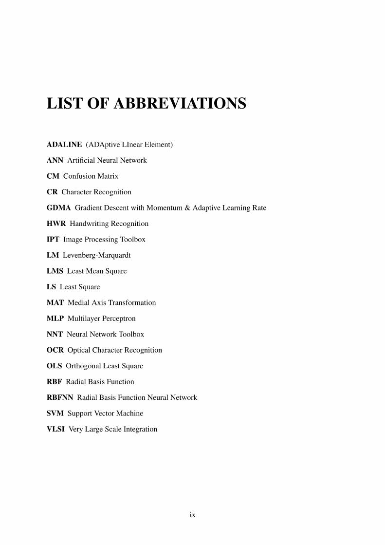
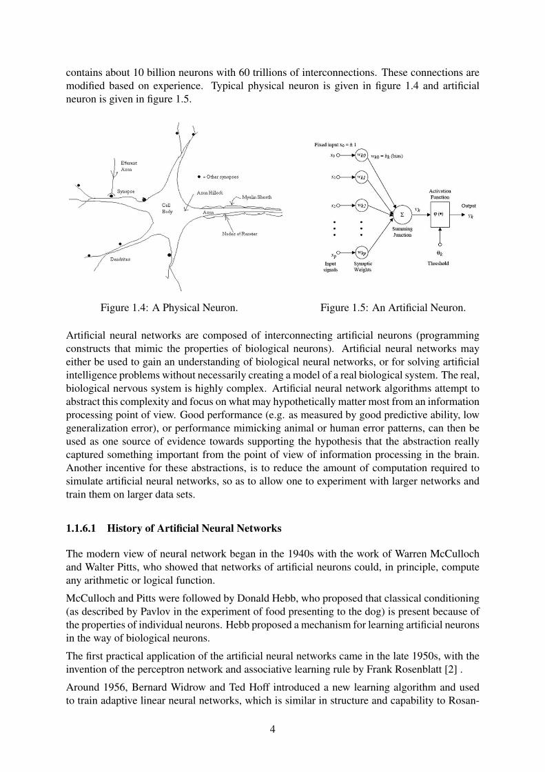
contains about 10 billion neurons with 60 trillions of interconnections. These connections aremodified based on experience. Typical physical neuron is given in figure 1.4 and artificialneuron is given in figure 1.5.

Figure 1.4: A Physical Neuron. Figure 1.5: An Artificial Neuron.

Artificial neural networks are composed of interconnecting artificial neurons (programmingconstructs that mimic the properties of biological neurons). Artificial neural networks mayeither be used to gain an understanding of biological neural networks, or for solving artificialintelligence problems without necessarily creating a model of a real biological system. The real,biological nervous system is highly complex. Artificial neural network algorithms attempt toabstract this complexity and focus on what may hypothetically matter most from an informationprocessing point of view. Good performance (e.g. as measured by good predictive ability, lowgeneralization error), or performance mimicking animal or human error patterns, can then beused as one source of evidence towards supporting the hypothesis that the abstraction reallycaptured something important from the point of view of information processing in the brain.Another incentive for these abstractions, is to reduce the amount of computation required tosimulate artificial neural networks, so as to allow one to experiment with larger networks andtrain them on larger data sets.

1.1.6.1 History of Artificial Neural Networks

The modern view of neural network began in the 1940s with the work of Warren McCullochand Walter Pitts, who showed that networks of artificial neurons could, in principle, computeany arithmetic or logical function.

McCulloch and Pitts were followed by Donald Hebb, who proposed that classical conditioning(as described by Pavlov in the experiment of food presenting to the dog) is present because ofthe properties of individual neurons. Hebb proposed a mechanism for learning artificial neuronsin the way of biological neurons.

The first practical application of the artificial neural networks came in the late 1950s, with theinvention of the perceptron network and associative learning rule by Frank Rosenblatt [2] .

Around 1956, Bernard Widrow and Ted Hoff introduced a new learning algorithm and usedto train adaptive linear neural networks, which is similar in structure and capability to Rosan-

4

blatt’s perceptron [3] . Another system besides perceptron was the (ADAptive LInear Ele-ment) (ADALINE) which was developed in 1960 by Widrow and Hoff (of Stanford Univer-sity).

Rosenblatt’s and Widrow’s network both suffer from limitation of applicability of networksonly to linearly seperable classes of problems. Limitations of these networks were publicizedin the book by Marvin Minsky and Seymour Papert with the fact that there were no powerfuldigital computers to do experiments. So, for a decade, neural network research was largelysuspended.

Development of neural network dramatically increased from 1980, as there were powerful per-sonal computers to do experiments and the development of multilayer backpropagation percep-tron network. The most influenced publication of the backpropagation algorithm was by DevidRumelhart and James Mclelland. This algorithm was the answer to the criticisms Minsky andPapert had made in the 1960s.

Significant progress has been made in the field of neural networks-enough to attract a great dealof attention and fund further research. Advancement beyond current commercial applicationsappears to be possible, and research is advancing the field on many fronts. Neurally based chipsare emerging and applications to complex problems developing. Clearly, today is a period oftransition for neural network technology.

1.1.6.2 Real Life Applications of Artificial Neural Networks

Some real life applications of Artificial Neural Network are given below.

• Signal processing (e.g. adaptive echo cancelling).

• Control (e.g. manufacturing plants for controlling automated machines).

• Robotics (e.g. vision recognition).

• Pattern recognition (e.g. recognizing handwritten characters).

• Medicine (e.g. storing medical records based on case information).

• Speech production (e.g.reading text aloud).

• Speech recognition.

• Vision (e.g. face recognition).

• Business (e.g. rules for mortgage decisions).

• Financial Applications (e.g. stock market prediction).

• Data Compression (e.g. images).

• Game Playing (e.g. chess).

1.2 Challenges

Unconstrained off-line handwriting recognition has significantly different writing styles andshapes. Shapes of the same character glyph vary across writers and even for the same writer.General handwritten text document can have large variations on writings. Same Character,

5

word or sentence can have different writing styles, alignment styles, skewness and slantnessfor the same document. It makes handwriting recognition more complicated.

Off-line handwritten text recognition can be seen as the most general case of handwriting recog-nition. Complexity of handwriting recognition system vary according to its problem domain (e.g., Number plate recognition, Cheque verification, Digit recognition, etc...). Writer Recog-nition is much more difficult than Writer Independent Handwriting Recognition. So, uncon-strained off-line handwriting recognition is a very challenging problem in the domain of patternrecognition and artificial intelligent.

1.3 Problem Definition

The high-level task of off-line handwriting recognition is to classify the ordered sequence ofimages of off-line characters. In this research work, problem of Nepali handwritten characterrecognition is addressed. This corresponds to the ability of human beings to recognize suchcharacters, which they are able to do with little or no difficulty. The recognition task is carriedout with Artificial Neural Network. Many geometric and statistical features are extracted fromimages so that the performance and accuracy of recognition system is achieved in the range ofhuman ability of recognition. The system performs character recognition by quantification ofthe character into a mathematical vector entity using the geometrical and statistical properties ofthe character image. The sub problems in the domain of off-line handwriting recognition suchas, noise removal, image binarization, object skeletonization, size normalization, etc. havegreat impact on recognition procedure. These sub-problems are also addressed with the mostsuitable solutions in the literature for this type of research work.

1.4 Objectives

The objective of this research is to investigate various feature extraction techniques and to com-pare Neural Network based pattern recognition techniques namely Multilayer Feed-forwardNetwork and Radial Basis Function Network. Comparative Performance matrices are analysed.The sub-problem field of off-line handwriting recognition is also addressed. Main objectivesare given below.

• To compare performance and efficiency of MLP and RBF Neural Networks on Off-lineNepali Handwriting Recognition Problem.

• To investigate Geometric and Statistical feature extraction techniques for off-line Nepalihandwritten text.

• To investigate preprocessing techniques (segmentation, skeletonization, normalization,etc.) for handwritten documents.

• To create benchmark databases for Nepali handwritten characters.

6

1.5 Contribution of this Thesis

The main contribution of this thesis to the field of Off-line Nepali Handwriting Recognition canbe seen in its extensive experimental work. A more detailed list of the various contributions isprovided below,

• Use of ANN to analysis the off-line handwriting recognition problem.

• Investigation of feature extraction techniques for off-line handwritten documents.

• Creation of Nepali Handwritten character database for the experimentation with therecognition system.

1.6 Outline of the Thesis

The remaining part of the document is organized as follows,

Chapter 2 describes the state of the art of the handwriting recognition. It includes the methodsand techniques used in the area of handwriting recognition till now.

Chapter 3 describes the Off-line Handwriting Recognition System architecture. The Top levelsystem overview along with sub-system engines are given with data flow directions.

Chapter 4 describes research methodologies used in the research. All the preprocessing, fea-ture extraction and recognition algorithms are described in this part of the document.

Chapter 5 describes the implementation of the system. It includes the techniques used for therealizations of the algorithms given in chapter 4.

Chapter 6 describes the corpus used in the evaluation of the purposed system. Off-line hand-writing recognition system is experimented with three self created Nepali handwritten characterdatasets for consonants, vowels and numerals respectively.

Chapter 7 describes the experimentation results of the recognition systems. Performance andefficiency of the proposed systems evaluated in Nepali handwritten character datasets are givenin this section.

Chapter 8 contains the summary and future scope of the research work.

7

Chapter 2

Literature Review

2.1 Previous Work

It is an ancient dream to make machines able to perform tasks like humans. The origin of char-acter recognition can actually be found back in 1870 as C.R. Carey of Boston Massachusettsinvented the retina scanner which was an image transmission system using a mosaic of pho-tocells. Two decades later the Polish P. Nipkow invented the sequential scanner which was amajor breakthrough both for modern television and reading machines. During the first decadesof the 19th century several attempts were made to develop devices to aid the blind through ex-periments with OCR. However, the modern version of OCR did not appear until the middle ofthe 1940’s with the development of the digital computer.

Before the age of digital computers, there was no such researches in the field of handwritingrecognition. The early researches after the digital age were concentrated either upon machine-printed text or upon a small set of well-separated handwritten text or symbols. Machine-printedCharacter Recognition (CR) generally used template matching and for handwritten text, low-level image processing techniques were used on the binary image to extract feature vectors,which were then fed to statistical classifiers [4].

CR research is somewhat limited until 1980 due to the lack of powerful computer hardware anddata perception devices. The period from 1980-1990 witnessed a growth in CR system devel-opment [5] due to rapid growth in information technology [6]. However, the CR research wasfocused on basically the shape recognition techniques without using any semantic information.This led to an upper limit in the recognition rate, which was not sufficient in many practicalapplications. Research progress on the off-line and on-line recognition during 1980-1990 canbe found in [7] and [8] respectively.

After 1990, image processing techniques and pattern recognition techniques were combined us-ing artificial intelligence. Along with powerful computers and more accurate electronic equip-ments such as scanners, cameras and electronic tablets, there came in efficient, modern useof methodologies such as artificial neural networks (ANNs), hidden Markov models (HMMs),fuzzy set reasoning and natural language processing.

Character segmentation from cursive handwritten documents is a difficult task. So in literaturemost of the researches were conducted on separated characters. Segmentation based approachfor isolated off-line Devanagari word recognition is described in [9]. Isolated Devanagari char-acter recognition with Regular Expressions & Minimum Edit Distance Method is described in

8

[10]. Research work [1] describes the template based Nepali alphanumeric handwriting recog-nition. Recent work on off-line devanagari character recognition carried out by Sharma et.al.(2006) uses quadratic classifiers for recognition and achieved 98.86% recognition accuracyfor devanagari numerals and 80.36% recognition accuracy for devanagari characters [11]. Re-search work [12] describes multiple classifier combination for Off-line Handwritten DevnagariCharacter Recognition and achieves 92.16% recognition accuracy for devanagari characters.Paper [13] compares Support Vector Machine (SVM) and ANN for off-line devanagari charac-ter recognition problem. Handwriting Recognition system based on cloud computing in givenin paper [14].

On Devnagari, a few techniques have been tested but no comparison of various recognitiontechniques available in literature is made. Also, there is lack of benchmark databases for Hand-written Devnagari Script to test the recognition systems. Only small lab experiments have beenfound in the literature.

Although research on recognizing isolated handwritten characters has been quite successful,recognizing off-line cursive handwriting has been found to be a challenging problem. There isa large corpus of research on the application of character recognition in different domains, butno system to date has achieved the goal of system acceptability.

2.2 Individual Character Recognition

Recognition of individual characters have greater recognition accuracy than the recognition ofwhole words. But the segmentation of individual characters from handwritten documents isa error prone task due to the unconstrained domain of handwritings. Among all individualcharacter recognition domains, individual digit recognition is much more researched. Due toconnectivity and smooth drawing properties, digit recognition has higher accuracy than otherhandwriting recognition domains. There are many researches in the domain individual char-acter recognition [5, 15, 16, 11, 1, 10, 17, 12, 13, 18, 19, 14, 20, 21]. Recognition algorithmsused for the recognition of individual characters includes the probability based approaches,statistical approaches, neural network based approaches, etc.

2.3 Word Recognition

Word-based recognition system determine the entire word without any attempt to segment orlocate individual characters. The methods used in word-based recognition are usually similarto those of character recognition.These approaches avoid the individual letter segmentationproblem. However, the whole word have higher writing variability than in the case of singlecharacter. Researches in the domain of word recognition are included in [6, 22, 9]

2.4 Preprocessing

For off-line handwriting recognition, most of the data is extracted from the scans of pages ofhandwritten text. The quality of these scanned pages is often poor due to scanning artifacts,noise or low resolution. From these text pages, text lines or single words have to be extractedfor recognition, non-text background like figures and other markings need to be ignored.

9

Depending on the captured image quality, the extracted text lines or words have to be pre-processed for further usage, for example, slant correction, skew correction, curve smoothing,size normalization, etc. Other preprocessing techniques include colour normalization, noiseremoval, image binarization, image skeletonization and components analysis for estimation ofpartial words and characters.

2.5 Feature Extraction

Feature extraction is one of the important stage of the handwriting recognition. Feature ex-traction is essential for efficient data representation and high recognition performance. A goodfeature set should represent the syntactic and semantic characteristic of a class that helps dis-tinguish it from other classes. We can have many different features that can be extracted frompreprocessed character images [23, 24, 25, 20].There are three major categories of feature extraction techniques:

• Geometrical and Topological Features: Extracting and Counting Topological Struc-tures, Geometrical Properties, Coding, Graphs, Trees, Strokes, Chain Codes etc.

• Statistical Features: Zoning, Crossing and Distances, Projections, Distribution mea-sures, etc.

• Global Transformation and Series Expansion Features: Fourier Transform, CosineTransform, wavelets, Moments, Karhuen-Loeve Expansion, etc.

2.6 Recognition Methods

There are large number of recognition techniques for the handwriting recognition problem[24]. The major category of recognition strategies are: template matching, statistical methods,structural methods, and neural networks.

2.6.1 Template Matching

Template matching techniques determine the degree of similarity between two vectors (pixeldistributions, shapes, curvatures, etc) in the feature space. Matching techniques can be groupedinto three classes: direct matching, deformable templates and elastic matching, and relaxationmatching. One of the most widely used technique for template matching is Dynamic Program-ming.

2.6.2 Statistical Techniques

Statistical methods are concerned with statistical decision functions and a set of optimal cri-teria, which determine the probability of the observed pattern belonging to a certain class. Instatistical representation, the input pattern is described by a feature vector. Statistical tech-niques use concepts from statistical decision theory to establish decision boundaries betweenpattern classes. There are several statistical techniques for handwriting recognition, such as,k-Nearest Neighbour, Hidden Markov Model, Fuzzy set reasoning, Support Vector Machine,etc.

10

2.6.3 Structural Techniques

In structural methods the handwritten characters are represented as unions of structural primi-tives. In the structural methods the character primitives extracted from handwriting are quan-tifiable, and one can find the relationship among them. Basically, structural methods can becategorized into two classes: grammatical methods and graphical methods.

2.6.4 Neural Network Techniques

A Neural Network is a computing structure consisting of a massively parallel interconnectionof artificial adaptive neurons. The main advantages of neural networks is its ability to be trainedautomatically from examples, good performance with noisy data, possible parallel implemen-tation, and efficient tools for learning large databases. There are many neural network basedrecognition techniques like multilayer perceprton, radial basis function, recurrent networks,self organizing maps, etc.

11

Input Character Preprocessed Feature Feature Output

Image Preprocessing Image Extraction Vector Recognition Character

Chapter 3

SYSTEM OVERVIEW

The Top level handwriting recognition system is divided into four sub-systems, image acquisi-tion, preprocessing, feature extraction and recognition. The top level model of proposed systemis given in Figure 3.1.

Figure 3.1: Off-line Handwriting Recognition System.

The basic system architecture of the image acquisition, preprocessing, feature extraction andrecognition is briefly described in section 3.1, section 3.2, section 3.3 and section 3.4, respec-tively.

3.1 Image Acquisition

Images are acquired by scanning the handwritten documents using digital scanners or by takingphotograph of the handwriting document using digital camera. CANON LIDE scanner is usedto scan the handwritten samples from different writers. Each images are scanned at 300dpi inRGB color mode. Detail of the handwritten corpus used for the experimentation is given inchapter 6. Figure 3.2 shows the slicing of off-line character images from handwritten samplesand Figure 3.3 shows the final stage of the image acquisition.

12

01;_~ </lv&CPT ~

01 ~ ~ ~ '" S ~ r ~

01~~K>( ~ Lolf

o 1~ ~ix£e .s i f

oq~~~~~LOrf

09 ~~~ ~ { & (J r 5'

o 9' cil ~ (~ ~ LO i :f

l~

f8

,p

Figure 3.2: Image Slicing.

Figure 3.3: Image Acquisition.

13

Raw Image Grayscale Grayscale Noise De-noised Image ImagI---

(RGB) Conversion Image Removal Image Segmentation

Preprocessed Image Normalized Size Inverted ImageImage Skeletonization Image Normalization Image Inversion ~

Binary

e

,--------..

Geometric Geometric-. Features Feature Vector

Preprocessed + Global FeatureImage Vector

Statistical Statistical-. Features Feature Vector

3.2 Image Preprocessing

Pre-processing is done prior to feature extraction algorithms. The raw images are subjected to anumber of preliminary processing steps to make it usable in the descriptive stages of characteranalysis. Pre-processing aims to produce clean document images that are easy for the Recog-nition systems to operate accurately. The block diagram of preprocessing system is given inFigure 3.4. Details of the each preprocessing steps is described in the section 4.1.

Figure 3.4: Image Preprocessing.

3.3 Feature Extraction

After pre-processing of the character images, feature vectors are extracted, which is used in thetraining and recognition stage. Feature sets play one of the most important roles in a recognitionsystem. A good feature set should represent characteristic of a class that helps distinguish itfrom other classes, while remaining invariant to characteristic differences within the class. Thehigh level block diagram of the feature extraction system is given in the Figure 3.5. Detaildescription of each feature extraction techniques is given in section 4.2.

Figure 3.5: Feature Extraction.

14

TrainingCorpus --1 MLP Neural 1 Network J MLP Trained

1Feature

Network J Weights I Network

Vector

--1 RBFNeural 1 Network j RBFTrainedNetwork J Weights I Network

Training

TestingCorpus MLP Trained Performance

Network Metric

TestingFeatureVector

RBFTrained Performance

Network Metric

3.4 Recognition

Recognition engine of the system consists of two neural network based algorithms implementedin it. There are two stages of the recognition, training and testing. In the training stage systemlearns how to behave in the new environment of similar inputs and in the testing stage accuracyof the classification is determined. The top level recognition system is given in figure 3.6.Detail of the each algorithms used in the recognition system is given in the section 4.3.

Figure 3.6: Training and Testing.

15

Chapter 4

RESEARCH METHODOLOGY

This chapter describes the theoretical concept behind the methods used in this research. Archi-tecture of the proposed handwriting recognition system is given in chapter 3. Subsections ofthis chapter are organized as follows.

Section 4.1 describes the image preprocessing techniques. Feature extraction techniques aredescribed in the section 4.2. System training and testing methods are described in the section4.3.

4.1 Image Preprocessing

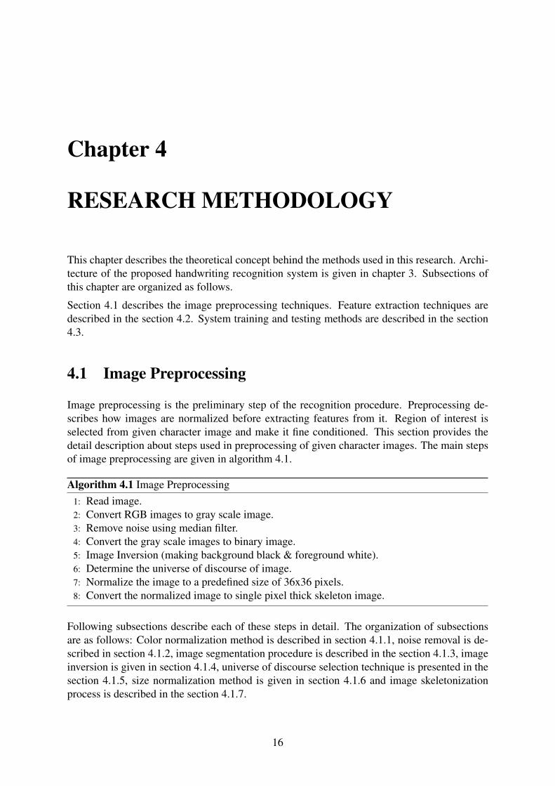
Image preprocessing is the preliminary step of the recognition procedure. Preprocessing de-scribes how images are normalized before extracting features from it. Region of interest isselected from given character image and make it fine conditioned. This section provides thedetail description about steps used in preprocessing of given character images. The main stepsof image preprocessing are given in algorithm 4.1.

Algorithm 4.1 Image Preprocessing1: Read image.2: Convert RGB images to gray scale image.3: Remove noise using median filter.4: Convert the gray scale images to binary image.5: Image Inversion (making background black & foreground white).6: Determine the universe of discourse of image.7: Normalize the image to a predefined size of 36x36 pixels.8: Convert the normalized image to single pixel thick skeleton image.

Following subsections describe each of these steps in detail. The organization of subsectionsare as follows: Color normalization method is described in section 4.1.1, noise removal is de-scribed in section 4.1.2, image segmentation procedure is described in the section 4.1.3, imageinversion is given in section 4.1.4, universe of discourse selection technique is presented in thesection 4.1.5, size normalization method is given in section 4.1.6 and image skeletonizationprocess is described in the section 4.1.7.

16

4.1.1 RGB to Grayscale Conversion

Given 24 bit true colour RGB image is converted into 8 bit grayscale image. Grayscale com-ponent is calculated by taking weighted summation of R, G and B components of RGB image.Weights are selected same as the NTSC color space selects for the luminance i.e. the grayscalesignal used to display pictures on monochrome televisions. For the RGB image f(x, y), corre-sponding graysclae image is given by,

g(x, y) = 0.2989 ∗R(f(x, y)) + 0.5870 ∗G(f(x, y)) + 0.1140 ∗B(f(x, y)) (4.1)

where, R(f(x, y)) is red component of the RGB image f(x, y), and so on.

Figure 4.1 shows the RGB to grayscale conversion of input image.

RGB Image Gray Image

Figure 4.1: RGB to Grayscale Conversion.

4.1.2 Noise Removal

Noise removal is one of the important step of image preprocessing. Any unnecessary pixelsare removed with the help of filtering. Non-linear median filtering technique is used for noiseremoval. Median filter is an effective method of noise removal which can suppress isolatednoise without blurring sharp edges. Median filter replaces a pixel with the median value of itsneighbourhood. For the digital image f(x, y), median filtered image is obtained as,

g(x, y) = median{f(i, j) (i, j) ∈ w} (4.2)

where, w is the neighbourhood centered around location (x, y) in the image. Figure 4.2 showsthe denoised image corresponding to given grayscaled image.

Gray Image Denoised Image

Figure 4.2: Noise Removal.

17

4.1.3 Image Segmentation

Segmentation is the central problem of distinguishing object from the background. There aremany algorithms for image segmentation. This section describes the thresholding method withOtsu’s threshold selection technique [26] for grayscale image segmentation.

Otsu’s graylevel threshold selection method for image binarization is a nonparametric and un-supervised method of automatic threshold selection. An optimal threshold is selected by thediscriminant criteria i.e., by maximizing the interclass variance between white and black pixels.Image segmentation algorithm for grayscale image is given in Algorithm 4.2. Figure 4.3 showsbinarized image of given grayscale image.

Denoised Image Binarized Image

Figure 4.3: Image Binarization.

Algorithm 4.2 Image Binarization1: Compute histogram and probability of each intensity level i , i = 1 · · ·L.2: Compute between class variance for black and white pixels, by taking threshold t = 1 · · ·L,3: σ2

b (t) = ω1(t)ω2(t)[µ1(t)− µ2(t)]2

where,

4: ω1(t) =t∑1

p(i) is the class probability for black pixels,

5: ω2(t) =L∑t+1

p(i) is the class probability for white pixels,

6: µ1(t) =t∑1

ip(i)ω1(t)

is the class mean for black pixels,

7: µ2(t) =L∑t+1

ip(i)ω2(t)

is the class mean for white pixels,

8: and, p(i) is the probability of intensity level i.9: Select t for which σ2

b (t) is maximum.10: Finally, binarize the grayscale image f(x, y) using the threshold t as,

11: g(x, y) =

{1 if f(x, y) ≥ t0 if f(x, y) < t

4.1.4 Image Inversion

Handwritten documents are normally written in white paper with black pen. For the recognitionsystem, we assume black pixels as a background and white pixels as the foreground. So,

18

captured images are inverted before passing into the recognition engine. The inverted image ofbinary image f(x, y) can be obtained by the negative transformation as,

g(x, y) = 1− f(x, y) (4.3)

Figure 4.4 shows the negative image of given binary image.

Binarized Image Inverted Image

Figure 4.4: Image Negatives.

4.1.5 Universe of Discourse

Determining universe of discourse of the character image is finding smallest rectangle thatencloses the character object. It removes extra pixels outside the convex hull of the characterimage. Figure 4.5 shows the discoursed image of given binary image.

Inverted Image Discoursed Image

Figure 4.5: Universe of Discourse.

4.1.6 Size Normalization

Size normalization is the technique of converting all the variable size input images to fixed sizeimages. Size normalization is done so that we do not require paddings of pixels at the time offeature extraction. All the input images are normalized to the predefined size of 36x36 pixels.Figure 4.6 shows the size normalized image.

4.1.7 Image Skeletonization

Skeletonization is a process for reducing object regions in a binary image to a skeletal remain-der that largely preserves the extent and connectivity of the original object while throwing away

19

Discoursed Image Size Normalized Image (36x36)

Figure 4.6: Size Normalization.

most of the original object pixels. It plays an important role in the preprocessing phase of hand-writing recognition. Skeletonization creates single pixel wide connected object boundary, thatpreserves euler number of the original object. There are many reasons behind skeletonizationof the binary image such as, to reduce the amount of data and time for processing the image, toextract critical features like end-points, intersection-points, connections etc., to help in shapeanalysis algorithms, and so on. Skeletonization calculates a medial axis skeleton so that pointsof this skeleton are at the same distance of its nearby borders. Image thinning algorithm is firstgiven by Harry Blum (1967) [27]. Binary image skeletonization is carried out by the objectthinning procedure that iteratively delete boundary points of a region object to the constraintsthat deletion of these points; (1) does not remove end points, (2) does not break connectivityand (3) does not cause excessive erosion of the region. Medial Axis Transformation (MAT)algorithm [28] for binary image thinning is given in algorithm 4.3. The MAT of a object regionhas an intuitive definition based on the so-called “prairie fire concept”. Consider an image re-gion, as a prairie of uniform dry grass, and suppose a fire it lit along its border. All fire frontswill advance into the region at the unique speed. The MAT of the object region is then the set ofpoints reached by more than one fire front at the same time. Figure 4.7 shows the skeletonizedimage of given binary image.

Algorithm 4.3 Image Skeletonization Algorithm1: Repeat following steps until no contour points.2: (a) Delete all contour points according to Definition 1.3: (b) Delete all contour points according to Definition 2.4: Definition 1: For contour point P1 (see table right for the 8- connected relationship) that

satisfies following conditions,(a) 2 ≤ N(P1) ≤ 6(b) T (P1) = 1(c) P2.P4.P6 = 0(d) P4.P6.P8 = 0

P9 P2 P3P8 P1 P4P7 P6 P5

Table: The 8- connected relationship

where N(P1) is the number of non-zero neighbours of P1: N(P1) =9∑i=2

Pi, and T (P1)

is the number of 0-1 transitions in the ordered sequence P2, P3, · · · , P9, P2 (clockwise).5: Definition 2: For contour point P1 that satisfies the following conditions

(a) same as above(b) same as above(c′) P2.P4.P8 = 0(d′) P2.P6.P8 = 0

20

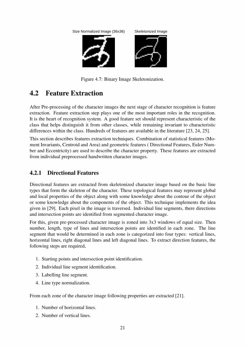
Size Normalized Image (36x36) Skeletonized Image

Figure 4.7: Binary Image Skeletonization.

4.2 Feature Extraction

After Pre-processing of the character images the next stage of character recognition is featureextraction. Feature extraction step plays one of the most important roles in the recognition.It is the heart of recognition system. A good feature set should represent characteristic of theclass that helps distinguish it from other classes, while remaining invariant to characteristicdifferences within the class. Hundreds of features are available in the literature [23, 24, 25].

This section describes features extraction techniques. Combination of statistical features (Mo-ment Invariants, Centroid and Area) and geometric features ( Directional Features, Euler Num-ber and Eccentricity) are used to describe the character property. These features are extractedfrom individual preprocessed handwritten character images.

4.2.1 Directional Features

Directional features are extracted from skeletonized character image based on the basic linetypes that form the skeleton of the character. These topological features may represent globaland local properties of the object along with some knowledge about the contour of the objector some knowledge about the components of the object. This technique implements the ideagiven in [29]. Each pixel in the image is traversed. Individual line segments, there directionsand intersection points are identified from segmented character image.

For this, given pre-processed character image is zoned into 3x3 windows of equal size. Thennumber, length, type of lines and intersection points are identified in each zone. The linesegment that would be determined in each zone is categorized into four types: vertical lines,horizontal lines, right diagonal lines and left diagonal lines. To extract direction features, thefollowing steps are required,

1. Starting points and intersection point identification.

2. Individual line segment identification.

3. Labelling line segment.

4. Line type normalization.

From each zone of the character image following properties are extracted [21].

1. Number of horizontal lines.

2. Number of vertical lines.

21

3. Number of Right diagonal lines.

4. Number of Left diagonal lines.

5. Normalized Length of all horizontal lines.

6. Normalized Length of all vertical lines.

7. Normalized Length of all right diagonal lines.

8. Normalized Length of all left diagonal lines.

9. Number of intersection points.

It results feature vector of dimensional 9 for each zone. A total of 81 (9x9) features are ob-tained.

4.2.2 Moment Invariant Features

Moment invariants are important tools in object recognition problem. These techniques grabthe property of image intensity function. Moment invariants were first introduced to the patternrecognition community in 1962 by Hu [30], who employed the results of the theory of algebraicinvariants and derived his seven famous invariants to rotation of 2-D objects. Moment invariantsused in this research for extracting statistical patterns of character images are given in [28].Moment invariants are pure statistical measures of the pixel distribution around the centre ofgravity of the character and allow capturing the global character shape information.

The standard moments mpq of order (p+ q) of an image intensity function f(x, y) is given by,

mpq =

∞∫−∞

∞∫−∞

xpyqf(x, y)dxdy p, q = 0, 1, 2, ... (4.4)

A uniqueness theorem states that if f(x, y) is piecewise continues and has non-zero values onlyin a finite part of the xvis, yvis plane, moments of all order exist and the moment sequence (mpq)is uniquely determined by f(x, y). Conversely, (mpq) is uniquely determines f(x, y).

For discrete domain, the 2-D moment of order (p+ q) for a digital image f(x, y) of size MxNis given by,

mpq =M−1∑x=0

N−1∑y=0

xpyqf(x, y) p, q = 0, 1, 2, ... (4.5)

The corresponding central moment of order (p+ q) is defined as,

µpq =M−1∑x=0

N−1∑y=0

(x− x)p(y − y)qf(x, y) p, q = 0, 1, 2, ... (4.6)

where,x =

m10

m00

and y =m01

m00

(4.7)

The normalized central moments, denoted by ηpq, are defined as,

ηpq =µpqµγ00

(4.8)

22

where,γ =

p+ q

2+ 1 for p+ q = 2, 3, ... (4.9)

A set of seven invariant moments can be derived from the second and third moments [30] whichare invariant to translation, scale change, mirroring, and rotation, are given as follows.

φ1 = η20 + η02 (4.10a)φ2 = (η20 − η02)2 + 4η211 (4.10b)φ3 = (η30 − 3η12)

2 + (3η12 − η03)2 (4.10c)φ4 = (η30 + η12)

2 + (η21 + η03)2 (4.10d)

φ5 = (η30 − 3η12)(η30 + η12)[(η30 − 3η12)2 − 3(η12 + η03)

2]

+ (3η21 − η03)(η21 + η03)[3(η30 + η12)2 − (η21 + η03)

2] (4.10e)φ6 = (η20 − η02)[(η30 + η12)

2 − (η21 + η03)2]

+ 4η11(η30 + η12)(η21 + η03) (4.10f)φ7 = 3(η21 − η03)(η30 + η12)[(η30 + η12)

2 − 3(η21 + η03)2]

+ 3(η12 − η30)(η21 + η03)[3(η30 + η12)2 − (η21 + η03)

2] (4.10g)

4.2.3 Euler Number

Euler number is the difference of number of objects and the number of holes in the image. Thisproperty is affine transformation invariant. Euler number is computed by considering patternsof convexity and concavity in local 2-by-2 neighbourhoods [31]. Euler number can be calcu-lated by using local information and does not require connectivity information. Calculating theEuler number of a binary image can be done by counting the occurrences of three types of 2x2binary patterns.

P1 =

(1 0 0 1 0 0 0 00 0 , 0 0 , 0 1 , 1 0

)

P2 =

(0 1 1 0 1 1 1 11 1 , 1 1 , 1 0 , 0 1

)P3 =

(1 0 0 10 1 , 1 0

)Let C1, C2 and C3 be the number of occurrences of patterns P1, P2 and P3 respectively, thenthe Euler Number for the image with 4- and 8-connectivity is simply given as [31],

E4 =1

4(C1− C2 + 2C3) (4.11)

E8 =1

4(C1− C2− 2C3) (4.12)

23

4.2.4 Normalized Area of Character Skeleton

The area of the object within the binary image is simply the count of the number of pixels inthe object for which f(x, y) = 1. Normalized regional area is the ratio of the number of thepixels in the skeleton of binary image to the total number of pixel in the image.

4.2.5 Centroid of Image

Centroid specifies the center of mass of the object region in given image. Horizontal centroidcoordinate is calculated by dividing the sum of all horizontal positions of the object whichare non zero with area of the object. Similarly, vertical centroid coordinate is calculated bydividing the sum of all vertical positions of the object which are non zero with area of theobject. Centroid coordinates of the binary image f(x, y) of size MxN are given in equation4.13,

centroidx =m10

m00

=

1

N

M−1∑i=0

N−1∑j=0

xjf(i, j)

M−1∑i=0

N−1∑j=0

f(i, j)

(4.13a)

centroidy =m01

m00

=

1

M

M−1∑i=0

N−1∑j=0

yjf(i, j)

M−1∑i=0

N−1∑j=0

f(i, j)

(4.13b)

4.2.6 Eccentricity

The eccentricity is the ratio of the distance between the foci of the ellipse that best fit thecharacter object and its major axis length. Eccentricity describes the rectangularity of the regionof the object. The measure of eccentricity can be obtained by using the minor and major axesof such an ellipse [32]. This method of calculating eccentricity uses the second order moments.The eccentricity of the ellipse is given by,

e =

√α2 − β2

α2(4.14)

where α and β are semi-major axis and semi-minor axis of the ellipse respectively, which aregiven by,

α =

√2[µ20 + µ02 +

√(µ20 − µ02)2 + 4µ2

11]

µ00

(4.15)

β =

√2[µ20 + µ02 −

√(µ20 − µ02)2 + 4µ2

11]

µ00

(4.16)

where µpq is as described in equation 4.6.

24

4.3 Training and Testing

After the feature extraction phase, process of training and testing begins. In the training phase,recognition system learns patterns of different classes from input feature vectors. The learningis done in supervised manner. After the training phase, system is ready to test in unknownenvironment. Recognition system is then tested against testing feature vectors and accuracyand efficiency of the system is calculated. In this research, recognition is carried out using twoneural network algorithms, multilayer feedforward neural network with Levenberg-Marquardt(LM) and Gradient Descent with Momentum & Adaptive Learning Rate (GDMA) learning andradial basis function networks with Orthogonal Least Square (OLS) learning. Section 4.3.1describes the MLP algorithm and section 4.3.2 describes the RBF algorithm.

4.3.1 Multilayer Feedforward Backpropagation Network

A multilayer feedforward neural network consists of a layer of input units, one or more layersof hidden units, and one layer of output units. A neural network that has no hidden unitsis called a Perceptron. However, a perceptron can only represent linear functions, so it isn’tpowerful enough for the kinds of applications we want to solve. On the other hand, a multilayerfeedforward neural network can represent a very broad set of non-linear functions. So, it isvery useful in practice. This multilayer architecture of Network determines how the input isprocessed. The network is called feedforward because the output from one layer of neuronsfeeds forward into the next layer of neurons. There are never any backward connections, andconnections never skip a layer. Typically, the layers are fully connected, meaning that all unitsat one layer are connected with all units at the next layer. So, this means that all input units areconnected to all the units in the layer of hidden units, and all the units in the hidden layer areconnected to all the output units.

Usually, determining the number of input units and output units is clear from the application.However, determining the number of hidden units is a bit of an art form, and requires experi-mentation to determine the best number of hidden units. Too few hidden units will prevent thenetwork from being able to learn the required function, because it will have too few degrees offreedom. Too many hidden units may cause the network to tend to over-fit the training data,thus reducing generalization accuracy.

Consider a multilayer feed-forward network as shown in Figure 4.8. The net input to unit I inlayer k + 1 is given by,

nk+1i =

Sk∑i=1

wk+1ij akj + bk+1

i (4.17)

where, Sk is the number of neurons in the kth layer, wk+1ij is the weight from jth neuron of

layer k to neuron i of the layer k + 1, akj is the output of neuron j from the layer k and bk+1i is

the bias connected to ith neuron in the layer k + 1.

The output of unit I will be,ak+1i = fk+1(nk+1

i ) (4.18)

where, fk+1(·) is the activation function (see appendix A.2) used in layer k + 1.

25

Input Layer Hidden Layer Output Layer

Figure 4.8: Feedforward Multilayer Perceptron.

For a M layer network the system equations in the matrix form are given by

a0 = p (4.19)

ak+1 = fk+1(W k+1ak + bk+1), k = 0, 1, 2, ...,M − 1 (4.20)

where, p is the input layer of the network.

The network learns association between a given set of input-output pairs (pi, ti), i = 1, 2, ..., Qfor Q number of training samples.

Now, next step of calculating feed forward quantities for all layers in the network is the backpropagation training. In this phase, we decide how neural network learn weights and biases withminimizing the generalization error. The quantity of weight and bias to adjust in the networkparameters is send back to network from output layer to first hidden layer. In this research work,Levenberg-Marquardt Backpropagation Learning and Gradient Descent with Momentum &Adaptive Learning Rate are applied for learning the network parameters. Levenberg-MarquardtBackpropagation Learning algorithm is described in the section 4.3.1.1 and Gradient Descentwith Momentum & Adaptive Learning rate algorithm is described in the section 4.3.1.2.

4.3.1.1 Levenberg-Marquardt Learning Algorithm

Many algorithms focus on standard numerical optimization, i.e, using alternative methods toheuristic based optimizations for computing the weights associated with network connections.The most popular algorithms for this optimization are the conjugate gradient and Newton’smethods. Newton’s method is considered to be more efficient in the speed of convergence,but its storage and computational requirements go up as the square of the size of the network.The LM algorithm is efficient in terms of high speed of convergence and reduced memoryrequirements compared to the two previous methods. In general, with networks that contain upto several hundred weights, the LM algorithm has the fastest convergence [33].

For LM , the performance index to be minimized is defined as,

F (w) =

Q∑p=1

K∑k=1

(tkp − akp)2 (4.21)

26

where, w = [w1 w2 w3 ... wN ]T consists of all the weights of the network (including bias), tkp isthe target value of the kth output and pth input pattern, akp is the actual value of the kth outputand pth input pattern, N is the number of weights, and K is the number of the network outputs.

Equation (4.21) can be written as,F (w) = ETE (4.22)

where E = [e11 ... eK1 e12 ... eK2 ... e1P ... eKQ]T ,

ekp = tkp − akp, k = 1, 2, ..., K, p = 1, 2, ..., Q where E is the cumulative error vector (for allinput patterns). From equation (4.22) the Jacobian matrix is defined as,

J =

∂e11∂w1

∂e11∂w2

... ∂e11∂wN

∂e21∂w1

∂e21∂w2

... ∂e21∂wN

... ... ... ...∂eK1

∂w1

∂eK1

∂w2... ∂eK1

∂wN

... ... ... ...∂e1Q∂w1

∂e1Q∂w2

...∂e1Q∂wN

∂e2Q∂w1

∂e2Q∂w2

...∂e2Q∂wN

... ... ... ...∂eKQ

∂w1

∂eKQ

∂w2...

∂eKQ

∂wN

(4.23)

The increment of weights ∆w at iteration t can be obtained as follows:

∆w = −(JTJ + µI)−1JTE (4.24)

where, I is identity matrix, µ is a learning parameter and J is Jacobian of K output errors withrespect to N weights of the neural network.

Now, network weights are calculated using the following equation,

wt+1 = wt + ∆w (4.25)

For µ = 0, it becomes the Gauss-Newton method. For very large value of µ the LM algorithmbecomes the steepest decent algorithm. The learning parameter µ is automatically adjusted ateach iteration to meet the convergence criteria. The LM algorithm requires computation of theJacobian matrix J at each iteration and inverse of JTJ matrix of dimension NxN . This largedimensionality of LM algorithm is sometimes unpleasant to large size neural network.

The learning parameter µ is updated in each iteration as follows. Whenever the F (w) valueis decreases, µ is multiplied by decay rate βinc, whenever, F (w) is increases, µ is divided bydecay rate βdec in new step.

The LM Back-propagation training is illustrated in the Algorithm 4.4.

27

Algorithm 4.4 Levenberg-Marquardt Back-propagation Algorithm1: Initialize the weights using Nguyen-Widrow weight initialization algorithm (see Appendix

A.1) and parameter µ.2: Compute the sum of the squared errors over all inputs F (w).3: Solve Eq.(4.24) to obtain the increment of weights.4: Recompute the sum of squared errors F (w) using w + ∆w as trial w, and adjust5: if trial F (w) ≤ F (w) in Step 2 then6: w = w + ∆w7: µ = µ.βinc8: Goto Step 2.9: else

10: µ = µβdec

11: Goto Step 4.12: end if

4.3.1.2 Gradient descent with momentum and adaptive learning rate

Gradient descent with momentum and variable learning rate is heuristic based optimizationtechnique, developed from an analysis of the performance of the standard steepest descentalgorithm, used for learning the feed-forward back-propagation neural network. It has a goodconvergence capacity than other heuristic based technique.

The term momentum controls feedback loop and help to overcome at the situation of noisygradient, so that local minima can be passed without stoking. Momentum Adds a percentage ofthe last movement to the current movement. Momentum allows a network to respond not onlyto the local gradient, but also to recent trends in the error surface.

The term adaptive learning rate plays important role for fast convergence. The learning rateautomatically changes while learning the patterns. For each iteration of learning, if the per-formance decreases toward the goal, then the learning rate is increased by the factor ηinc. Ifthe performance increases by more than the factor ηmax inc, the learning rate is adjusted by thefactor ηdec and the change that increased the performance is not made.

To learn the association between a given set of input-output pairs (pi, ti), i = 1, 2, ..., Q for Qnumber of training samples, the performance index (given in Eq.4.21) should be minimized.

The gradient of error function is the partial derivative of error function with respect to networkweights and biases. It is given as,

∇F =δF

δwkij(4.26)

Change in weight for iteration t+ 1 is given by,

∆w(t+ 1) = µ∆w(t) + (1− µ)η∇F (4.27)

where, µ is the momentum constant and η is the learning rate.

Now, Weight is adjusted by,

w(t+ 1) = w(t) + ∆w(t+ 1) (4.28)

28

Input Layer RBF Layer Output Layer

R

~ '---------~--------~Slxl 51 S2xl

4.3.2 Radial Basis Function Network

Radial-basis function network is used to perform a complex pattern classification task, the prob-lem basically solved by transforming it into a high dimensional space in a non-linear manner.Non linear separability of complex patterns is justified by Cover’s theorem,which stated as, “Acomplex pattern-classification problem cast in a high dimensional space non-linearly is morelikely to be linearly separable than in a low-dimensional space”.

Radial basis functions are embedded into a two layer feed-forward network. Such a network ischaracterized by a set of inputs and set of outputs. In between the inputs and outputs, there is alayer of processing units called hidden units. Each of them implements a radial basis function.Generally, there is a single hidden layer. In pattern classification problem, inputs representfeature values, while each output corresponds to a class. A general RBF Neural NetworkArchitecture is given in Figure 4.9.

Figure 4.9: RBF Neural Network.

Let the input vector x = [x1, x2, ..., xR]T is feed to RBF Network. The network output can beobtained by,

tk =M∑j=1

wkjφj(x) + bk (4.29)

where φj(·) denotes the radial basis function of the jth hidden neuron, wkj denotes the hidden-to-output weight from jth hidden neuron to kth output neuron, bk denotes the bias connected tokth output neuron, and M denotes the total hidden neurons.

A radial basis function is a multidimensional function that describes the distance between agiven input vector and a pre-defined centre vector. There are different types of radial basisfunction. A normalized Gaussian function usually used as a radial basis function, which isgiven as,

φj(x) = exp(−‖x− µj‖2

2σ2j

) (4.30)

where, µj and σj denote the centre and spread width of the jth neuron, respectively.

Generally, the Radial Basis Function Neural Network (RBFNN) training can be divided intotwo stages:

29

1. Determine the parameters of radial basis functions, i.e., Gaussian centre and spreadwidth.

2. Determine the output weight w with supervised learning method. Usually Least MeanSquare (LMS).

The first stage is very crucial, since the number location of centres in the hidden layer willinfluence the performance of the RBF neural network directly. In the next section, the principleand procedure of self-structure RBF algorithm will be described.

4.3.2.1 Orthogonal Least Square Training Algorithm

Orthogonal Least Squares is the most widely used supervised algorithm for radial basis neuralnetwork training. OLS is a forward stepwise regression procedure. Starting from a large pool ofcandidate centres, i.e., from training examples, OLS sequentially selects the centre that resultsin the largest reduction of sum-square-error at the output.

For M basis vectors Φ = (φ1, φ2, ..., φM), orthogonal set Q = (q1, q2, ..., qM) can be derivedwith the help of Grahm-Schmidt orthogonalization procedure as follows:

q1 = φ1 (4.31)

αik =qTi φkqTi qi

1 ≤ i ≤ k (4.32)

qk = φk −k−1∑i=1

αikqi (4.33)

for k = 2, 3, ...,M

The orthogonal set of basis vectors Q is linearly related to the original set Φ by the relationshipΦ = QA [34], where A is upper triangular matrix given by,

A =

1 α12 ... α1M

0 1 ...... αM−1,M0 ... 0 1

(4.34)

Using this orthogonal representation, the RBF solution is expressed as,

T = ΦW = QG (4.35)

and the Least Square (LS) solution for the weight vector G in the orthogonal space is,

G = (QTQ)−1QTT (4.36)

Since Q is orthogonal, QTQ is then diagonal and each component of G can be extracted inde-pendently without ever having to compute a pseudo-inverse matrix as,

gi =qTi T

qTi qi(4.37)

30

The sum of squares of the target vector T is given as,

T TT =M∑i=1

g2i qTi qi + ETE (4.38)

OLS select a subset of regressors in stepwise forward manner by selecting the regressor qi,whichcontributes to reduction of the error (relative to the total T TT ) by,

[err]i =g2i q

Ti qi

T TT(4.39)

The summary of Orthogonal Least Square RBF training [34] is given in Algorithm 4.5.

Algorithm 4.5 OLS Algorithm1: At the first step,for 1 ≤ i ≤M , compute2: Orthogonalize vector: q(i)1 = φi

3: Compute LS Solution: g(i)1 =q(i)T

1 T

q(i)T

1 q(i)1

4: Compute error reduction: [err](1)i =

g(i)2

1 q(i)T

1 q(i)1

TTT

5: select regressor that yields highest reduction in error q1 = argq(i)1

max[err](i)1 = φi1

6: At the kth step, for 1 ≤ i ≤M , and i not already selected

7: Orthogonalize vector: α(i)jk =

qTj φi

qTj qj, q

(i)k = φi −

k−1∑i=1

α(i)jk qj , for1 ≤ j ≤ k

8: Compute LS Solution: g(i)k =q(i)T

k T

q(i)T

k q(i)k

9: Compute error reduction: [err](i)k =

g(i)2

k q(i)T

k q(i)k

TTT

10: select regressor qk = argq(i)k

max[err](i)k = φik −

k−1∑j=1

αjkqj

11: Stop at iteration M if residual error falls below pre-specified threshold ε

12: 1−M∑j=1

[err]j ≤ ε

13: The regressors {φi1 , φi2 , · · · , φiM} define the final subset of RBF centers.

4.3.3 Performance Metrics

Performance of the recognition systems is evaluated on the basis of the metrics described below:

1. Recognition Rate: Number of instances that were classified correctly out of the totalinstances.

2. Misclassification Rate: Number of instances that were classified incorrectly out of thetotal instances.

3. Model Build Time: Time taken to train a classifier on a given data set.

31

Chapter 5

IMPLEMENTATION

All the algorithms of purposed handwriting recognition system are implemented in MATLAB®version 7.13.0.564 (R2011b). MATLAB is installed on a Intel(R) Core(TM)2 Duo CPUT6500 @ 2.10GHz processor. The Computer has total main memory of 2 Gigabyte and 32-bitMicrosoft Windows 7 Ultimate operating system installed in it.

5.1 MATLAB

The name MATLAB stands for MATrix LABoratory. MATLAB is high-level technical com-puting language having high-performance computation. MATLAB started life in the 1970sas a user-friendly interface. It integrates computation, visualization, and programming in aneasy-to-use environment where problems and solutions are expressed in familiar mathematicalnotation. MATLAB has very wide range of applications and can now be used as a very sim-ple and transparent programming language where each line of code looks very much like themathematical statement it is designed to implement. Typical uses of the MATLAB are givenbelow.

• Mathematical and scientific computation.

• Algorithm development.

• Application development, including Graphical User Interface building.

• Data analysis, exploration and visualization.

• Modelling, simulation and prototyping.

• Graphics, in 2D and 3D, including colour, lighting and animation.

MATLAB is an interactive system whose basic data element is an array that does not requiredimensioning. This allows solving many technical computing problems, especially those withmatrix and vector formulations, in a fraction of the time it would take to write a program ina scalar non-interactive language such as C or FORTRAN. In university environments, it isthe standard instructional tool for introductory and advanced courses in mathematics, engineer-ing and science. In industry, MATLAB is the tool of choice for high-productivity research,development and analysis.

32

The reason behind using MATLAB for my research work experimentation is its wide varietyand flexible toolboxes. Toolboxes are comprehensive collections of MATLAB functions (M-files) that extend the MATLAB environment to solve particular classes of problems. In thisresearch work, mainly image processing toolbox and neural network toolbox are used alongwith other basis functionality of the MATLAB.

5.2 Image Processing Toolbox

Image Processing Toolbox (IPT) is very rich MATLAB toolbox for working with images. It in-cludes many powerful and very efficient image processing functions. It provides a comprehen-sive set of standard algorithms and graphical tools for image processing, analysis, visualizationand algorithm development. We can use IPT to perform complex image processing tasks likeimage enhancement, image deblurring, feature detection, noise reduction, image segmentation,geometric transformations, image registration, etc. Many toolbox functions are multithreadedto take advantage of multicore and multiprocessor computers.

Here, IPT is used for image preprocessing techniques like noise removal, segmentation, skele-tonization, etc. and for some feature extraction techniques (eg. euler number). It is also usedfor visualizing and analysing the results of image preprocessing and feature extraction steps.

5.3 Neural Network Toolbox

Neural Network Toolbox (NNT) provides tools for designing, implementing, visualizing, andsimulating neural networks. Neural networks are composed of simple elements operating inparallel. These elements are inspired by biological nervous systems. As in nature, the networkfunction is determined largely by the connections between elements. We can train a neuralnetwork to perform a particular function by adjusting the values of the connections betweenelements. Neural networks are used for applications where formal analysis would be difficultor impossible, such as pattern recognition, identification, classification, speech, vision and con-trol systems. Neural Network Toolbox supports feedforward networks, radial basis networks,dynamic networks, self-organizing maps, and other proven network paradigms. NNT providesvery customizable neural network functions which we can adjust according to our need. Atypical neural network training contains following steps:

1. Loading data source.

2. Selecting attributes required.

3. Decide training, validation, and testing data.

4. Data manipulations and Target generation.

5. Neural Network creation and initialisation.

6. Network Training and Testing.

7. Performance evaluation.

In this research, NNT is used for multilayer feedforward backpropagation network and radialbasis function network training algorithms.

33

5.4 Feature Vector Creation

Global feature vector is created according to the algorithms described in the section 4.2. Let usconsider image shown in figure 5.1. The binary matrix of this skeletonized image is given infigure 5.2.

Figure 5.1: Nepali consonant letter ’ka’. Figure 5.2: Letter ’ka’ as binary matrix.

5.4.1 Directional Feature Vector

For the directional feature extraction, image is zoned into 3x3 sub-images. Figure 5.3 showszoned images of image given in the figure 5.1.

zone11 zone12 zone13

zone21 zone22 zone23

zone31 zone32 zone33

Figure 5.3: Zoned images

Normalized feature vectors corresponding to each zone are given in Table 5.1.

34

zone11 feature vector [-1,-1,-1,-1,-1,-1,-1,-1,-1]zone12 feature vector [0.80,1,1,1,0.85,0,0,0,1]zone13 feature vector [0.80,1,1,1,0.85,0,0,0,1]zone21 feature vector [1,1,0.80,1,0,0,0.86,0,1]zone22 feature vector [0.60,0.80,0.80,0.80,0.63,0.03,0.06,0.03,0.40]zone23 feature vector [1,1,1,0.80,0,0,0,0.80,1]zone31 feature vector [0.80,1,1,1,0.90,0,0,0,1]zone32 feature vector [0.80,0.80,1,1,0.58,0.25,0,0,1]zone33 feature vector [1,1,0.80,1,0,0,0.87,0,1]

Table 5.1: Directional feature vectors corresponding to figure 5.3.

5.4.2 Moment Invariant Feature Vector

Moment invariant features are extracted from whole character image. It implements the algo-rithm given in section 4.2.2. Moment invariant features corresponding to figure 5.1 are givenbelow,

[ 1.3937, 0.1858, 0.8792, 0.0024, 0.0001, 0.0009, -0.0001]

5.4.3 Euler Number Feature Vector

There is a single entry for Euler number in global feature vector. An Euler number correspond-ing to figure 5.1 is 0.

5.4.4 Normalized Area of Character Skeleton Feature Vector

There is a single entry for normalized area of character image in global feature vector. Nor-malized area corresponding to figure 5.1 is 0.0841. Normalized area is calculated by followingformula.

normalized area = 1− area

image size

5.4.5 Centroid Feature Vector

Centroid is also extracted from whole character image. There are two entries for centroid inglobal feature vector. Normalized centroid corresponds to figure 5.1 is given below,

[0.9857, 0.9860]

5.4.6 Eccentricity Feature Vector

There is single entry in global feature vector for eccentricity. Eccentricity corresponds to figure5.1 is 0.6870.

35

5.4.7 Global Feature Vector

Global feature vector is created by appending all above feature vectors to a single feature vector.There is 93 dimensional global feature vector for each character images. The global featurecorresponds to figure 5.1 is given below,

input vector=[ -1, -1, -1, -1, -1, -1, -1, -1, -1, 0.80, 1, 1, 1, 0.85, 0, 0, 0, 1, 0.80, 1, 1, 1, 0.87, 0,0, 0, 1, 1, 1, 0.80, 1, 0, 0, 0.86, 0, 1, 0.60, 0.80, 0.80, 0.80, 0.63, 0.03, 0.07, 0.03, 0.40, 1, 1, 1,0.80, 0, 0, 0, 0.80, 1, 0.80, 1, 1, 1, 0.90, 0, 0, 0 1, 0.80, 0.80, 1, 1, 0.58, 0.25, 0, 0, 1, 1, 1, 0.80,1, 0, 0, 0.87, 0, 1, 0.999, 0.999, 0.999, 0.999, 0.999, 0.999, 1.00, 0, 0.08, 0.98, 0.98, 0.69].

To create target vector corresponding to above global feature vector, we create a vector withdimensionality equal to output classes. For figure 5.1, since it belongs to Nepali consonantclass, we have 36 dimension target vector with first entry equal to 1 and all other entries equalto 0. So, the target vector corresponds to figure 5.1 is given by,

target vector=[1, 0, 0, 0, 0, 0, 0, 0, 0, 0, 0, 0, 0, 0, 0, 0, 0, 0, 0, 0, 0, 0, 0, 0, 0, 0, 0, 0, 0, 0, 0, 0,0, 0, 0, 0].

Now, above feature vector along with corresponding target vector is ready to feed into neu-ral network for training and testing. Training is done in supervised manner with two neuralnetwork algorithms, MLP and RBF networks.

36

Chapter 6

NEPALI HANDWRITTEN DATASETS

To do experimentation with this research work, benchmark datasets for Off-line Nepali Hand-written Characters are created. There are three separate datasets for Nepali handwritten con-sonants, vowels and numerals. The overall dataset creation procedure is discussed in section6.1. More detail about Nepali consonant dataset, vowel dataset and numeral dataset is givenin the section 6.2, section 6.3 and section 6.4, respectively. Training and testing samples forrecognition system are selected from each dataset in certain ratio.

6.1 Dataset Creation Procedure

Datasets are created by taking handwriting samples from different writers from different fields.The overall procedure for creating off-line Nepali handwritten character datasets is describedin the Algorithm 6.1.

Algorithm 6.1 Handwritten Dataset Creation1: Take handwritten samples from different writers in A4 paper.2: Scan the sample documents using digital scanner.3: Slice and crop individual characters from each documents.4: Make individual directory for each category of datasets.5: Make individual class directory in each dataset directory.6: Drag individual characters in the corresponding class directory.7: Datasets are ready.

37

6.2 Nepali Handwritten Consonant Dataset

Nepali language contains 36 different Devanagari alphabets for Consonants. Figure 6.1 showsNepali handwritten consonants. To create training and testing dataset of Nepali handwrittenconsonants, handwritten consonant images are scanned with digital scanner and cropped forindividual characters.

Nepali handwritten consonant dataset contains total 7380 image samples. Samples are takenfrom 45 different writers from different fields. Each class of consonant dataset contains 205images with varying styles and shapes.

Figure 6.1: Nepali Handwritten Consonants.

6.3 Nepali Handwritten Vowel Dataset

Nepali language contains 12 different Devanagari alphabets for vowels. Figure 6.2 showsNepali handwritten vowels. To create training and testing dataset of Nepali handwritten vow-els, handwritten vowel samples are scanned with digital scanner and cropped for individualcharacters.

Nepali handwritten vowel dataset contains total 2652 image samples. Samples are taken from44 different writers from different fields. Each class of vowel dataset contains 221 images withvarying styles and shapes.

Figure 6.2: Nepali Handwritten Vowels.

38

6.4 Nepali Handwritten Numeral Dataset

Nepali language contains 10 different Devanagari numerals. Figure 6.3 shows Nepali hand-written numerals. To create training and testing dataset of Nepali handwritten numerals, hand-written numeral images are scanned with digital scanner and cropped for individual characters.

Nepali handwritten numeral dataset contains total 2880 image samples. Samples are taken from45 different writers from different fields. Each class of numeral dataset contains 288 imageswith varying styles and shapes.

Figure 6.3: Nepali Handwritten Numerals.

39

Chapter 7

EXPERIMENTATIONS AND RESULTS

The aim of this research work was to evaluate the complete MLP and RBF neural networkhandwriting recognition systems. Experiment is done with off-line isolated Nepali handwrittenalphabets and numerals. There are three separate datasets for Nepali consonants, vowels andnumerals. First of all, system is trained in each dataset using different random samples fromeach dataset in supervised manner. And then system is tested against new samples and accuracyis measured. In every datasets the data was partitioned into three parts, for training, validationand testing. Every set has completely different samples, which are selected randomly in uni-formly manner from the pool of given dataset. Experimentation with each recognition systemsis carried out five times in each datasets. The accuracy and efficiency for each datasets is theaverage of all the experimentation results for that dataset. Feature vectors used for training andtesting is as described in section 5.4. The network configurations and recognition results forMLP and RBF handwriting recognition systems for each datasets are described in this chapter.

Table 7.1 shows neural network configurations for all three datasets on MLP and RBF recog-nition systems. Training and testing samples are uniformly distributed random samples. Theremaining samples in each datasets other than training and testing samples are used as valida-tion samples. Validation is used for generalization and early stopping the recognition systemwhile training.

Dataset Dataset Size Recognition Train/Test Hidden Layer No. ofName (Class * Samples) Algorithm Samples Neurons Epochs

Numeral 10 * 288 MLP (LM) 2016/432 30 9Dataset = 2880 RBF 2304/576 580 580Vowel 12 * 221 MLP (LM) 1857/397 30 12Dataset = 2652 RBF 2122/530 840 840

Consonant 36 * 205 MLP (GDMA) 5411/891 100 1000Dataset = 7380 RBF 5166/891 1025 1025

Table 7.1: Neural Network Configurations.

40

100

Table 7.2 shows performance matrices for MLP and RBF based off-line handwriting recogni-tion systems on each datasets. The best recognition result is obtained with RBF based recog-nition system on off-line Nepali numeral dataset. In each datasets the RBF based recognitionsystem outperforms MLP based recognition system. Training time, recognition accuracy andmiss-classification rates for each dataset experimentation are given in Table 7.2.

Dataset Recognition Training Recognition Miss-classificationName Algorithm Time (min.) Accuracy (%) Rate (%)

Numeral MLP 16.66 87.50 12.50Dataset RBF 69.91 94.44 5.55Vowel MLP 24.36 79.15 20.85Dataset RBF 113.23 86.04 13.96

Consonant MLP 13.92 71.72 28.28Dataset RBF 308.4 80.25 19.75

Table 7.2: Recognition Results.

Figure 7.1 shows the graph of recognition system accuracy on all three datasets.

Figure 7.1: Recognition Accuracy of Off-line Handwriting Recognition Systems.

Figure 7.2 shows the graph of training time for each recognition systems in each datasets.

41

350

300

250

~ 200

]."E

150;:

100

50

o

Figure 7.2: Training Time of Off-line Handwriting Recognition Systems.

Table 7.3 shows individual recognition results for Nepali handwritten numeral dataset for eachclasses. The corresponding Confusion Matrix (CM) for test set of numeral dataset is given intable 7.4. The numeral test set contains 576 random samples for testing. Here, CM is an 10x10matrix with CM(i, j) is the number of target samples of the ith class classified by the outputsinto class j.

Class Recognition Recognition Class Recognition RecognitionAlgorithms Accuracy (%) Algorithms Accuracy (%)

MLP 97.7 MLP 94.1RBF 98.6 RBF 98.4MLP 85.1 MLP 82.1RBF 93.0 RBF 90.4MLP 82.5 MLP 82.5RBF 98.0 RBF 81.1MLP 82.9 MLP 86.7RBF 95.0 RBF 96.2MLP 97.8 MLP 80.4RBF 100 RBF 90.9

Table 7.3: Recognition Results For Individual Numerals.

Figure 7.3 shows the graph of recognition accuracy for each classes of numeral dataset.

42

0 q :t. s }!{ 4- t» T s0q:t..s}!{

f

4-LoTs

100

90 r-- :-- :-- r--

l:80 r-- r-- - - r-- r-- - -

~70 r-- r-- - - r-- r-- r-- r-- - -

j 60 r-- r-- - - r-- r-- r-- r-- - -50 l- I- - - r- l- I- I- - -

j40 r-- r-- - - r-- r-- r-- r-- - -~..

I- r-- - - r- l- I- I- - -8 30Ii

20 r-- r-- - - r-- r-- r-- r-- - -10 r-- r-- - - r-- r-- r-- r-- - -

0"0" "," "~" "~" "y" "~" "~" "b" "C "\"

I·MLP 97.7 94.1 85.1 82.1 82.5 82.5 82.9 86.7 97.8 80.4

I. RBF 98.6 98.4 93 90.4 98 81.1 95 96.2 100 90.9

Class69 0 0 0 0 0 0 0 0 10 61 0 0 0 0 1 0 0 00 0 53 4 0 0 0 0 0 00 0 3 47 0 0 2 0 0 00 0 0 0 49 1 0 0 0 00 0 5 3 1 43 0 0 0 10 1 0 0 0 0 57 1 0 00 0 0 0 1 0 1 51 0 00 0 0 0 0 0 0 0 64 00 1 1 1 0 1 1 0 0 50

Table 7.4: Confusion Matrix of Numeral Dataset Testing.

Figure 7.3: Recognition Accuracy of Each Numeral Classes.

Table 7.5 shows individual recognition results for Nepali handwritten vowel dataset for eachclasses. The corresponding CM for test set of vowel dataset is given in table 7.6. The voweltest set contains 530 random samples for testing. Here, CM is an 12x12 matrix with CM(i, j)is the number of target samples of the ith class classified by the outputs into class j.

Figure 7.4 shows the graph of recognition accuracy for each classes of vowel dataset.

Table 7.7 shows individual recognition results for Nepali handwritten consonant dataset foreach classes. The corresponding CM for test set of consonant dataset is given in table 7.8 andtable 7.9 . The consonant test set contains 891 random samples for testing. Here, CM is an36x36 matrix with CM(i, j) is the number of target samples of the jth class classified by theoutputs into class i.

Figure 7.5 shows the graph of recognition accuracy for each classes of consonant dataset.

43

~.•

oy-~.,

100

90

~ 80 r-- - - r-1:" 70 f- - - f- - - f- f- - f-- ~e 60 r- - - r- - - r- r- - r- ~§" 50 f- - - f- - - f- f- - f- ~e.g 40 f- - - f- - - f- f- - f- -.';;.. 30 f- - - f- - - f- f- - f- -8~ 20 f- - - f- - - f- f- - f- ~

10 f- - - f- - - f- f- - f- ~0

"3(' "3IT" "s" "~' "3" "3''' "v' "1)'" "3IT" "3ft" ":if' "31:"

I·MlP 77.8 93.5 84.2 88.5 75.8 85.2 78.4 82.9 71.4 64.7 64.1 86.5

I.RBF 78.9 87.8 81.1 90.5 92.1 87.8 97.6 85.7 76.5 80 76.1 88.5

()y- ~.•

Class Recognition Recognition Class Recognition RecognitionAlgorithms Accuracy (%) Algorithms Accuracy (%)

MLP 77.8 MLP 93.5RBF 78.9 RBF 87.8MLP 84.2 MLP 88.5RBF 91.1 RBF 90.5MLP 75.8 MLP 85.2RBF 92.1 RBF 87.8MLP 78.4 MLP 82.9RBF 97.6 RBF 85.7MLP 71.4 MLP 64.7RBF 76.5 RBF 80.0MLP 64.1 MLP 86.5RBF 76.1 RBF 88.5

Table 7.5: Recognition Results For Individual Vowels.

Class45 6 0 0 0 4 0 0 1 0 1 03 36 0 0 0 0 0 0 0 1 0 10 0 51 0 1 0 0 0 1 1 2 00 0 2 38 0 0 0 1 0 0 1 01 0 2 0 35 0 0 0 0 0 0 02 0 0 0 1 36 0 0 0 0 0 21 0 0 0 0 0 40 0 0 0 0 01 0 0 0 0 0 2 36 2 0 1 00 0 0 0 0 0 0 1 26 5 2 00 0 0 0 0 0 0 0 6 32 2 01 0 0 2 0 0 0 1 5 2 35 01 3 0 0 0 0 0 0 0 2 0 46

Table 7.6: Confusion Matrix of Vowel Dataset Testing.

Figure 7.4: Recognition Accuracy of Each Vowel Classes.

44

Class Recognition Recognition Class Recognition RecognitionAlgorithms Accuracy (%) Algorithms Accuracy (%)

MLP 94.1 MLP 78.3RBF 94.1 RBF 91.3MLP 80.8 MLP 51.9RBF 92.3 RBF 77.8MLP 60.0 MLP 84.6RBF 64.0 RBF 84.6MLP 66.7 MLP 73.1RBF 77.8 RBF 80.8MLP 65.4 MLP 59.4RBF 73.1 RBF 68.8MLP 96.3 MLP 63.6RBF 92.6 RBF 72.7MLP 76.9 MLP 91.7RBF 88.5 RBF 91.7MLP 85.0 MLP 92.3RBF 90.0 RBF 96.2MLP 50.0 MLP 64.0RBF 72.7 RBF 76.0MLP 75.0 MLP 36.8RBF 79.2 RBF 38.8MLP 87.5 MLP 72.4RBF 100 RBF 86.2MLP 75.9 MLP 63.6RBF 75.9 RBF 90.9MLP 66.7 MLP 44.0RBF 73.3 RBF 56.0MLP 89.3 MLP 66.7RBF 82.1 RBF 77.8MLP 73.9 MLP 80.0RBF 78.3 RBF 91.4MLP 76.0 MLP 55.2RBF 80.0 RBF 79.3MLP 88.2 MLP 60.0RBF 82.4 RBF 72.0MLP 73.1 MLP 64.0RBF 76.9 RBF 80.0

Table 7.7: Recognition Results For Individual Characters.

45

Class16 0 0 0 1 0 0 0 1 0 0 0 0 0 0 0 0 10 21 0 0 0 0 0 0 1 0 0 0 0 1 0 0 0 00 0 24 0 0 0 0 0 0 1 0 0 0 0 1 0 0 00 0 0 21 0 1 0 0 0 0 0 0 0 0 0 0 1 00 0 0 0 16 0 0 0 0 0 0 0 1 0 0 0 0 00 0 0 0 0 22 0 0 0 0 0 0 0 0 0 0 0 00 0 0 1 0 0 14 0 0 0 1 0 0 0 0 0 0 20 0 0 0 1 0 0 21 0 1 0 0 0 0 0 0 0 00 0 0 0 0 0 1 0 19 0 0 0 0 0 0 0 0 00 0 0 0 0 0 0 3 0 22 0 0 0 0 0 0 0 00 0 0 0 0 0 0 0 0 0 25 0 0 0 0 0 0 00 0 0 0 0 0 0 0 0 0 0 16 0 0 0 0 0 10 0 0 0 2 0 0 0 0 0 0 1 23 1 0 0 0 00 0 0 0 1 0 1 0 0 0 0 1 0 22 0 0 0 10 0 0 0 0 0 0 0 0 0 0 0 0 0 18 0 0 00 0 0 0 0 0 0 0 0 0 0 0 0 0 0 25 0 00 0 0 1 0 0 0 0 0 0 0 0 0 0 0 0 16 00 0 0 0 1 0 0 0 0 0 0 2 0 0 0 0 0 190 0 0 1 0 1 0 0 0 0 0 1 0 0 1 0 2 00 0 0 0 0 0 0 0 0 0 0 0 0 0 0 0 0 00 0 0 2 0 0 0 0 0 0 0 0 0 0 0 1 1 00 0 0 0 0 0 0 0 1 0 0 0 0 0 0 0 0 00 0 0 0 0 0 0 0 0 2 0 0 0 0 0 0 1 00 0 0 0 0 0 0 0 0 1 0 0 0 0 0 0 0 00 0 1 0 0 0 0 0 0 2 0 1 0 0 0 0 0 00 0 0 0 0 1 0 0 0 0 0 0 0 0 0 0 1 10 0 0 0 0 0 0 0 0 0 0 0 1 0 0 0 0 00 0 0 0 0 0 0 0 0 0 0 0 0 0 0 0 0 00 0 0 1 1 1 0 0 0 0 0 0 1 0 0 0 0 00 0 1 0 2 0 0 0 1 0 0 0 0 0 0 0 0 01 0 0 0 0 0 0 0 0 0 0 0 0 0 0 0 0 00 1 0 0 0 0 1 0 1 0 0 0 0 0 0 0 0 00 0 0 0 0 0 1 0 0 0 1 0 0 0 0 0 0 00 1 0 0 0 0 0 0 1 0 0 0 0 0 0 0 0 00 0 0 0 0 0 0 1 0 3 0 0 0 0 0 0 0 00 0 0 0 0 0 0 1 1 0 0 0 0 0 0 0 0 0

Table 7.8: Confusion Matrix (I) of Consonant Dataset Testing.

46

Class0 0 0 0 1 0 0 0 0 0 0 0 0 0 0 0 1 00 0 0 0 0 0 0 0 0 0 0 0 0 0 0 0 0 00 1 0 0 0 0 0 1 0 0 0 0 0 0 0 1 2 01 0 0 0 0 0 0 0 0 0 0 0 0 0 0 0 0 00 0 0 0 0 0 0 0 0 0 0 0 0 0 0 0 0 01 0 0 0 0 0 0 1 1 0 0 0 0 0 0 0 1 00 0 0 0 0 0 0 0 0 0 0 0 2 0 0 0 0 00 1 0 0 0 0 2 1 0 0 0 0 0 0 0 0 2 00 0 0 2 0 0 0 0 0 0 0 0 0 0 0 0 0 00 2 0 0 0 1 1 0 0 0 0 0 0 0 0 1 0 00 0 0 0 0 0 0 0 1 0 0 0 0 0 0 0 0 00 0 0 0 1 0 0 0 0 1 0 0 0 0 0 0 0 00 0 0 0 0 0 0 0 0 0 0 0 0 0 0 0 0 00 0 0 0 0 0 1 0 0 0 0 0 0 0 1 0 0 00 0 0 1 0 0 0 2 0 1 1 0 1 0 0 0 0 00 2 0 0 0 0 0 1 1 1 0 0 0 0 0 0 0 01 0 0 0 1 0 0 0 1 0 0 1 2 0 0 1 0 10 0 0 0 2 0 0 0 0 0 1 0 0 0 0 0 0 0

19 0 0 0 0 0 0 0 0 0 0 0 0 0 0 0 0 00 7 0 0 0 0 0 0 0 0 0 0 0 0 0 1 0 00 0 24 1 0 1 2 3 0 0 0 0 0 0 1 0 0 00 0 0 25 0 0 0 0 0 0 0 0 0 0 0 0 0 00 0 0 0 22 0 0 0 0 0 1 1 0 0 0 1 0 11 0 0 0 0 20 0 1 0 0 0 0 0 1 0 1 0 00 2 0 0 1 0 22 0 0 0 0 0 0 2 0 0 0 00 0 0 0 0 0 0 14 0 0 0 0 0 0 0 0 0 00 1 0 0 0 0 0 0 23 0 0 0 0 0 0 0 0 00 1 0 0 0 0 0 1 0 14 0 0 0 0 0 0 0 20 1 0 0 1 0 0 0 0 0 18 1 0 0 0 0 0 01 0 0 0 0 0 0 0 0 0 0 32 0 2 0 0 0 00 0 0 0 0 0 0 0 0 0 0 0 20 0 1 0 0 00 0 0 0 0 0 0 0 0 0 0 0 0 23 0 1 0 00 0 0 0 0 0 0 0 0 0 1 0 0 0 14 0 0 00 0 0 0 0 0 0 0 0 0 1 0 0 1 0 18 0 00 0 0 0 0 0 2 0 1 0 0 0 0 0 0 0 20 10 1 0 0 0 0 0 0 0 1 0 0 0 0 0 0 0 20

Table 7.9: Confusion Matrix (II) of Consonant Dataset Testing.

47

100

90

80

i 70 l- I-,.

60i!~< 50 -coil~ 40..8Ii. 30

20

10

0¥Y~YYYYYYY~YYY~YV~VYYYYYYYYYYYVyyyyy

I·MlP 94 78 81 52 60 85 67 73 65 59 96 64 77 92 86 92 50 64 75 37 88 72 76 64 57 44 89 67 74 80 76 55 88 60 73 64

InSF 94 91 92 78 64 85 78 81 73 69 93 73 89 92 90 96 73 76 79 39 10 86 76 91 73 56 82 78 78 91 80 79 82 72 77 80

Figure 7.5: Recognition Accuracy of Each Consonant Classes.

48

Chapter 8

CONCLUSION

8.1 Conclusion

Off-line handwriting recognition with neural network is presented and evaluated on Nepalihandwritten alphabet and numeral datasets. Two neural network based supervised classificationmethods (MLP and RBF) are experimented. The important preprocessing steps and featureextraction techniques for segmented characters are also described in full detail.

Off-line Nepali Handwritten Character recognition is a difficult problem, not only because ofthe great amount of variations in human handwriting, but also because of the overlapped andjoined characters. Recognition accuracy of the system greatly depends upon the nature of thedata to be recognized.

For the experimentation with the purposed off-line Nepali handwriting recognition system, selfcreated off-line Nepali handwritten character datasets are used. Three are three well populatedhandwritten datasets for Nepali numerals, vowels and consonants respectively. All datasets areso created that, it can also be used as writer identification and document verification research.Nepali handwritten numeral dataset contains total 2880 image samples with 288 samples foreach 10 classes of Nepali numerals, Nepali handwritten vowel dataset contains total 2652 im-age samples with 221 samples for each 12 classes of Nepali vowels and Nepali handwrittenconsonant dataset contains 7340 image samples with 205 samples for each 36 classes of Nepaliconsonants.

Off-line Nepali handwriting recognition system evaluated on Off-line Nepali numeral datasetgives best accuracy of 94.44% over all other datasets. In other datasets, due to high varia-tions on writing styles, shapes and cursive nature of characters, the recognition accuracy isdecreases. But, very encouraging results are obtained while experimentation on all datasets.For Off-line Nepali vowel dataset, recognition accuracy of 86.04% is obtained and for off-lineNepali consonant dataset, recognition accuracy of 80.25% is obtained. In all cases, RBF basedrecognition system outperforms MLP based recognition system. RBF based recognition enginetakes little more time for training but gives a very encouraging results while testing.

Recognition accuracy is directly proportional to the set of good features. So, feature extrac-tion engine is the most important part of the recognition system. Good features describe theproperty of character image very well, which ultimately helps in learning well the recognitionengine the particular pattern. For extracting good features from character image, it should bewell pre-processed. So, pre-processing is also very important step of recognition. This re-search describes two very important category of feature extraction techniques: geometry based

49

features and pixel distribution based features. Geometric features are very good descriptors ofimages for capturing physical shape of objects and statistical features are also very importantand necessary descriptors for capturing the pixel distribution of the object.

To further improve the quality of recognition system the combination of the proposed methodswith additional preprocessing and feature extraction techniques are recommended. Especially,features extracting methods for shape informations which contain the semantic properties ofthe object have great impact on the efficiency of the recognition system.

8.2 Future Scope

Handwriting recognition is the research topic over past four decades, different methods havebeen explored by a large number of researchers to recognize characters. Various approacheshave been proposed and tested in different parts of the world, including statistical methods,structural and syntactic methods and neural networks. No handwriting recognition system iscent percent accurate till now. The recognition accuracy of the neural networks proposed inthis research work can be further improved. Large training corpus with varying writing stylescan help in good generalization of the system. The future scope of this research is given below:

• Proposed system can be tested with known handwritten datasets like Germana database,IAM database, MNIST database, CEDAR database etc.

• Experimentation can be enhanced by taking other spatial domain features along withfrequency domain features.

• Purposed system can be extended for the recognition of words, sentences and documents.

• Purposed system can be extended for multilingual character recognition.

50

Appendix A

Neural Network Parameters

A.1 Nguyen–Widrow Weights Initialization

ANN uses learning algorithms to train the weights and biases of the network. We normallychoose random values as initial weights for the network. The random choice of initial weightsand biases will affect the performance and efficiency of the learning algorithms. If the averageperformance of the algorithm is required, a test using several different sets of initial weightsand biases will be carried out. Good choice of initial weights and biases in the training phaseof the experiments greatly impact the performance of the network training. The chosen initialweights determine the starting point in the error landscape, which controls whether the learningprocess will end up in a local minimum or the global minimum. The easiest method is to selectthe weights randomly from suitable range such as between [-1.0 1.0] or minmax(input range).More sophisticated approach for selecting the initial weights for the network training is theNguyen-Widrow weight initialization technique.

Nguyen-Widrow weight initialization technique calculates the interval from which the weightsare taken in accordance with the number of input neurons and the number of hidden neurons[35]. Nguyen-Widrow weight initialization algorithm is given in algorithm A.1.

Algorithm A.1 Nguyen-Widrow Weight Initialization Algorithm1: Calculate parameter β using,2: β = 0.7 ∗ p 1

n

3: where p = number of hidden units and4: n = number of input units5: Calculate weight wij as,

6: wij = β ∗ wij(random)

‖wj(random)‖

A.2 Activation Function

A activation function (also known as transfer function) determines the relation between inputand output. Activation function normalizes the output value to certain range. There are number

51

tanh

+1

v

-1

of activation functions in use with neural networks. Activation functions may be linear or non-linear. Some of the widely used activation functions are McCulloch-Pitts thresholding function,piecewise-linear function and sigmoid function.

Sigmoid function has s-shaped graph and is most common form of activation function for defin-ing the output of a neuron. Sigmoid function is strictly increasing, continuous and differentialfunction. It exhibits a graceful balance between linear and nonlinear behaviour. An example ofthe sigmoid function is the logistic function, defined by,

φ(v) =1

1 + exp(−av)(A.1)

where, a is the slope parameter of the sigmoid function and v is the local output of the neuron.

Hyperbolic tangent sigmoid activation function is symmetric bipolar activation function, de-fined by,

φ(v) =2

(1 + exp(−2v))− 1 (A.2)

The graph of hyperbolic tangent sigmoid activation function is given in figure A.1.

Figure A.1: Hyperbolic tangent sigmoid activation function.

52

Appendix B

Sample Source Codes

source codes are omitted for now · · ·

53

References

[1] K. C. Santosh and C. Nattee, “Template-based nepali handwritten alphanumeric charac-ter recognition,” Thammasat International Journal of Science and Technology (TIJSAT),Thammasat University, Thailand, vol. 12, no. 1, 2007.

[2] S. Haykin, Neural Networks: A Comprehensive Introduction. Prentice Hall, 1999.

[3] M. T. Hagan, H. B. Demuth, and M. Beale, Neural Network Design. pub-PWS:adr: PWS-Kent Publishing Company, Division of Wadsworth, Inc., 1996.

[4] C. Y. Suen, M. Berthod, and S. Mori, “Automatic recognition of handprinted characters:The state of the art,” Proceedings of IEEE, vol. 68, pp. 469–487, Apr. 1980.

[5] V. K. Govindan and A. P. Shivaprasad, “Character recognition: A review,” Pattern Recog-nition, vol. 23, no. 7, pp. 671–683, 1990.

[6] R. M. Bozinovic and S. N. Srihari, “Off-line cursive script word recognition,” IEEE Trans.Pattern Analysis and Machine Intelligence, vol. 11, pp. 68–83, Jan. 1989.

[7] S. Mori, C. Y. Suen, and K. Yamamoto, “Historical review of OCR research and develop-ment,” Proceedings of IEEE, vol. 80, pp. 1029–1058, July 1992.

[8] C. C. Tappert, C. Y. Suen, and T. Wakahara, “The state of the art in on-line hand-writing recognition,” IEEE Transactions on Pattern Analysis and Machine Intelligence,vol. PAMI-12, pp. 787–808, Aug. 1990.

[9] B. Shaw, S. K. Parui, and M. Shridhar, “Offline handwritten devanagari word recognition:A segmentation based approach,” in ICPR, pp. 1–4, 2008.

[10] P. S. Deshpande, L. Malik, and S. Arora, “Fine classification & recognition of hand writ-ten devnagari characters with regular expressions & minimum edit distance method,” JCP,vol. 3, no. 5, pp. 11–17, 2008.

[11] N. Sharma, U. Pal, F. Kimura, and S. Pal, “Recognition of off-line handwritten devnagaricharacters using quadratic classifier,” in Indian Conference on Computer Vision, Graphicsand Image Processing, pp. 805–816, 2006.

[12] S. Arora, D. Bhattacharjee, M. Nasipuri, D. K. Basu, and M. Kundu, “Multiple classifiercombination for off-line handwritten devnagari character recognition,” June 30 2010.

[13] S. Arora, D. Bhattacharjee, M. Nasipuri, L. Malik, M. Kundu, and D. K. Basu, “Perfor-mance comparison of SVM and ANN for handwritten devnagari character recognition,”June 30 2010.

54

[14] Y. Gao, L. Jin, C. He, and G. Zhou, “Handwriting character recognition as a service: Anew handwriting recognition system based on cloud computing,” in ICDAR, pp. 885–889,IEEE, 2011.

[15] C. Kan and M. D. Srinath, “Invariant character recognition with zernike and orthogonalfourier-mellin moments,” Pattern Recognition, vol. 35, pp. 143–154, Jan. 2002.

[16] H. Bunke, “Recognition of cursive roman handwriting - past, present and future,” In7th Int. Conf. on Document Analysis and Recognition, Edinbourgh, Scotland, vol. 01,pp. 7448–459, 2003.

[17] I. A. Lawal, R. E. Abdel-Aal, and S. A. Mahmoud, “Recognition of handwritten ara-bic (indian) numerals using freeman’s chain codes and abductive network classifiers,” inICPR, pp. 1884–1887, IEEE, 2010.

[18] J. Ashok and E. G. Rajan, “Off-line handwritteen character recognition suing radial basisfunction,” int. J. Advanced Networking and Applications, vol. 02, pp. 792–795, 2011.

[19] V. J. Dongre and V. H. Mankar, “A review of research on devnagari character recognition,”CoRR, vol. abs/1101.2491, 2011.

[20] N. VenkateswaraRao, A. Shrikhna, B. RaveendraBabu, and G. R. M. Babu, “An efficientfeature extraction and classification of handwritten digits using neural networks,” Inter-national Journal of Computer Science, Engineering and Applications (IJCSEA), vol. 1,Oct. 2011.

[21] D. D. Gaurav and R. Ramesh, “A feature extraction technique based on character geome-try for character recognition,” CoRR, vol. abs/1202.3884, 2012.

[22] A. Vinciarelli, “A survey on off-line cursive word recognition,” Pattern Recognition,vol. 35, pp. 1433–1446, July 2002.

[23] O. D. Trier, A. K. Jain, and T. Taxt, “Feature-extraction methods for character-recognition: A survey,” Pattern Recognition, vol. 29, pp. 641–662, Apr. 1996.

[24] A. K. Jain, R. P. W. Duin, and J. Mao, “Statistical pattern recognition: A review,” IEEETrans. Pattern Analysis and Machine Intelligence, vol. 22, pp. 4–37, Jan. 2000.

[25] D. Zhang and G. Lu, “Review of shape representation and description techniques,” PatternRecognition, vol. 37, no. 1, pp. 1–19, 2004.

[26] N. Otsu, “A threshold selection method from gray level histograms,” IEEE Trans. Sys-tems, Man and Cybernetics, vol. 9, pp. 62–66, Mar. 1979. minimize intra and inter classvariance.

[27] H. Blum, “A Transformation for Extracting new Descriptors of Shape,” in Models forthe Perception of Speech and Visual Form (Wathen-Dunn, ed.), pp. 362–380, MIT-Press,1967.

[28] R. C. Gonzalez and R. E. Woods, Digital Image Processing, Third Edition. Prentice Hall,2008.

55

[29] M. Blumenstein, B. Verma, and H. Basli, “A novel feature extraction technique for therecognition of segmented handwritten characters,” in ICDAR, pp. 137–141, 2003.

[30] M.-K. Hu, “Visual pattern recognition by moment invariants,” IRE Transactions on Infor-mation Theory, vol. IT-8, pp. 179–187, 1962.

[31] W. K. Pratt, Digital Image Processing (2nd Edition). New York, New York: John Wiley& Sons, Inc., 1991.

[32] P. L. Rosin, “Measuring rectangularity,” Mach. Vis. Appl, vol. 11, no. 4, pp. 191–196,1999.

[33] M. T. Hagan and M. B. Menhaj, “Training feedforward networks with the Marquardtalgorithm,” IEEE Transactions on Neural Networks, vol. 5, pp. 989–993, Nov. 1994.

[34] S. Chen, C. F. N. Cowan, and P. M. Grant, “Orthogonal least squares learning algorithmfor radial basis function networks,” IEEE Trans. on Neural Networks, vol. 2, pp. 302–309,1991.

[35] D. Nguyen and B. Widrow, “Improving the learning speed of 2-layer neural networks bychoosing initial values of the adaptive weights,” in IEEE International Joint Conferenceon Neural Networks (4th IJCNN’90), vol. III, (San Diego), pp. III–21–III–26, IEEE, 1990.Stanford.

56